treatment effect estimation with unconfounded assignment ...kr10/slides_fars_2012.pdf · treatment...

TREATMENT EFFECT ESTIMATION WITHUNCONFOUNDED ASSIGNMENT

Jeff WooldridgeMichigan State UniversityFARS Workshop, Chicago

January 6, 2012

1. Introduction2. Basic Concepts3. The Key Assumptions: Unconfoundedness and Overlap4. Identification of the Average Treatment Effects5. Estimating the Treatment Effects6. Panel Data7. Applications to Accounting8. Assessing Unconfoundedness9. Assessing and Improving Overlap

1

1. Introduction

∙What kinds of questions can we answer using a “modern” approach to

treatment effect estimation?

1. Does using a Big 4 auditing firm affect the quality of audits?

2. Does using a talent agent affect CEO compensation?

3. Do CEO equity incentives affect the incidence of accounting

irregularities?

2

∙ The main issue in treatment effect estimation concerns the nature of

the assignment, intervention, or “treatment.”

∙ Is the “treatment” randomly assigned? Rarely in accounting

applications. Can we assume the decision of whether to use a Big 4

firm is independent of all other factors (observed and unobserved)? Is

using equity incentives unrelated to other factors that affect accounting

irregularities?

3

∙Without experimental data cannot assume random assignment. With

observational (or retrospective) data, it may be reasonable to assume

that treatment is effectively randomly assigned conditional on

observable covariates.

∙ Called “unconfoundedness” or “ignorability” of treatment or

“selection on observables.” Sometimes called “exogenous treatment.”

4

∙ Does assignment depend fundamentally on unobservables, where the

dependence cannot be broken by controlling for observables?

∙ Called “confounded” assignment or “selection on unobservables” or

“endogenous treatment.”

∙ Often there is a self-selection component to treatment assignment

based on factors researchers cannot observe. Firms decide which

auditing firm to use or how to structure CEO compensation.

5

∙ Three situations:

(1) Assume unconfoundedness of treatment, and then explore how to

exploit it in estimation. (Leads to regression, propensity score, and

matching methods.)

(2) Allow self-selection on unobservables and exploit exogenous

instrumental variables. (Switching regression.)

(3) Exploit a “regression discontinuity” design, where the treatment (or

its probability) is determined as a discontinuous function of an

observed “forcing” variable.

∙ This workshop focuses on (1).

6

∙ The canonical setup is where there is a pre-treatment period and then

an intervention, where some units are subjected to the treatment. The

pre-treatment observables are used as controls to predict treatment

assignment.

∙ Other scenarios, including panel data, can be handled, but one must

be clear in defining the treatement effects and the nature of

unconfoundedness assumptions.

7

∙ KEY POINT: Under unconfoundedness, regression methods identify

treatment effect parameters, just as do propensity score weighting and

matching approaches.

∙ Propensity score methods are not a panacea for the self-selection

problem. They suffer systematic bias in cases where standard

regression methods do.

∙ Practically, matching methods seem to work better than regression

and weighting methods in some situations.

8

∙ Unconfoundedness is fundamentally untestable without extra

information – just as with standard regression analysis. (After OLS

estimation, we generally have no way of deciding whether the

explanatory variables are “exogenous” without outside information.)

∙ In some cases there are ways to assess the plausibility of

unconfoundedness, or study sensitivity of estimates.

9

∙ A second key assumption is “overlap,” which concerns the similarity

of the covariate distributions for the treated and control subpopulations.

It plays a key role in any of the estimation methods based on

unconfoundedness. In cases where parametric models are used, it can

be too easily overlooked.

∙ If overlap is weak, may have to redefine the population of interest in

order to precisely estimate a treatment effect on some subpopulation.

10

Caution Concerning Data Structures

∙ Standard methods for estimating ATEs are derived for a

cross-sectional setting (possibly with controls that are lagged

outcomes).

∙ Panel data must be treated carefully. At a minimum, time series

dependence must be accounted for in inference (not easily done with

matching). There are conceptual issues, such as matching firms across

time.

∙With panel data, a standard “fixed effects” analysis may be more

convincing, depending on how unconfoundedness is used.

11

2. Basic Concepts

Counterfactual Outcomes and Parameters of Interest

∙ Assume a binary treatment W – so two possible states of the world,

W 0 and W 1.

∙ For each population unit, two potential outcomes: Y0 (the outcome

without treatment) and Y1 (the outcome with treatment).

∙ Y0 and Y1 can be discrete, continuous, or some mix.

12

∙ Y0 is CEO compensation without using a talent agent, Y1 is

compensation using an agent. (Continuous response.)

∙ Y0 is binary indicator of whether there is an accounting irregularity

using a non-Big 4 firm, Y1 is the indicator using a Big 4 firm.

13

∙ The gain from treatment is

Y1 − Y0. (1)

∙ For a particular unit i, the gain from treatment is

Yi1 − Yi0. (2)

If we could observe these gains for a random sample, the problem

would be easy: just average the gain across the random sample.

14

∙ Key Problem: For each unit i, only one of Yi0 and Yi1 is

observed.

∙ In effect, we have a missing data problem. We will assume a random

sample of units from the population, but we do not observe both

outcomes.

15

∙ Two parameters are of primary interest. The average treatment

effect (ATE) is

ate EY1 − Y0. (3)

The expected gain for a randomly selected unit from the population.

∙ The average treatment effect on the treated (ATT) is the average

gain for those who actually were treated:

att EY1 − Y0|W 1 (4)

16

∙With heterogeneous treatment effects – that is, Yi1 − Yi0 not

constant – ate and att can be very different. ATE averages across gain

from units that might never be subject to treatment.

∙ IMPORTANT POINT: ate and att are defined without reference to a

model or discussion of the nature of the treatment. These definitions

hold when whether assignment is randomized, unconfounded, or

endogenous.

17

∙ How we estimate ate and att depends on what we assume about

treatment assignment.

∙We will also define ATEs and ATTs conditional on a set of observed

covariates. Some approaches to estimating ate and att rely on first

estimating conditional average treatment effects.

∙ Occasionally it is helpful to define average treatment effects in a

sample, for example,

sate N−1∑i1

N

Yi1 − Yi0.

18

Sampling Assumptions

∙ Assume independent, identically distributed observations from the

underlying population.

∙We would like to have Yi0,Yi1 : i 1, . . . ,N, but we only

observe Wi,Yi : i 1, . . . ,N, where

Yi 1 − WiYi0 WiYi1 Yi0 WiYi1 − Yi0 Yi0 Wi Gaini

(5)

19

∙ Random sampling rules out treatment of one unit having an effect on

other units. So the “stable unit treatment value assumption,” or

SUTVA, is in force: one unit’s treatment status has no effect on another

unit’s outcome.

∙ Random sampling across all observations rules out panel data.

20

Estimation under Random Assignment

∙ Strongest form of random assignment: Y0,Y1 is independent of

W. Then

EY|W 1 − EY|W 0 EY1 − EY0 ate att (6)

∙ EY|W 1 and EY|W 0 can be estimated by using sample

averages on the two subsamples.

ate Y1 − Y0.

∙ The randomization of treatment needed for the simple

difference–in-means estimator to consistently estimate the ATE is rare

in practice.

21

Many Treatment Levels

∙ If the treatmentWi takes on G 1 levels numbered 0, 1, . . . ,G, it is

straightforward to extend the counterfactual framework. Simply let

Y0, . . . ,YG denote the counterfactual outcomes associated with each

level of treatment.

∙Many estimation methods extend directly.

22

∙ Define the counterfactual means as

g EYg.

∙ The expected gain in going from treatment level g − 1 to g is

g − g−1.

∙ If Y0 is the response under no treatment then g − 0 is the average

gain of treatment level g relative to no treatment.

23

3. The Key Assumptions: Unconfoundedness and Overlap

∙ Rather than assume random assignment, for each unit i we also draw

a vector of covariates, Xi. Let X be the random vector representing the

population distribution.

∙ The strongest form of unconfoundedness: Conditional on X, the

counterfactual outcomes are independent of W.

∙ In other words, for units in the subpopulation defined by X x,

assignment is randomized.

24

A.1. Unconfoundedness: Conditional on a set of covariates X, the pair

of counterfactual outcomes, Y0,Y1, is independent of W:

Y0,Y1 W ∣ X, (7)

where the symbol “” means “independent of” and “∣” means

“conditional on.”

∙ Can also write unconfoundedness, or ignorability, as

DW|Y0,Y1,X DW|X, (8)

where D| denotes conditional distribution.

25

∙ Unconfoundedness is controversial. It underlies standard regression

methods to estimating treatment effects (via a “kitchen sink” regression

that includes the treatment indicator along with controls).

∙ Essentially, unconfoundedness leads to a difference-in-means after

adjusting for observed covariates.

∙ Even if we doubt we have “enough” of the “right” covariates, we

probably would attempt such a comparison.

26

∙ A weaker version of unconfoundedness:

A.1′. Unconfoundedness in Conditional Mean:

EYg|W,X EYg|X, g 0, 1. (9)

∙ Seems unlikely that this weaker version of the assumption holds

without the stronger version. With weaker version, mean effects on

different transformations of Yg not identified.

27

∙ IMPORTANT: Unconfoundedness is generally violated if X includes

variables that are themselves affected by the treatment.

∙ For example, in studying whether hiring a talent agent affects CEO

compensation, should not include in X variables possibly affected by

“treatment,” such as number of job interviews.

28

∙ An extreme case is where Y0,Y1 is independent of W but X is

not independent of W. (Think of assignment being randomized but then

X includes a post-assignment variable that can be affected by the

treatment.)

∙ Can show that unconfoundedness generally fails unless

EYg|X EYg, g 0, 1. (10)

∙ Bottom line: It is not always better to put everything possible in X.

29

∙ A compelling argument in favor of an analyisis based on

unconfoundedness is that the quantities we need to estimate are

nonparametrically identified. By contrast, instrumental variables

methods are either limited in what parameter they estimate or impose

functional form and distributional restrictions.

∙ Can write down simple economic models where unconfoundedness

holds, but the models limit the information available to agents when

choosing “participation.”

30

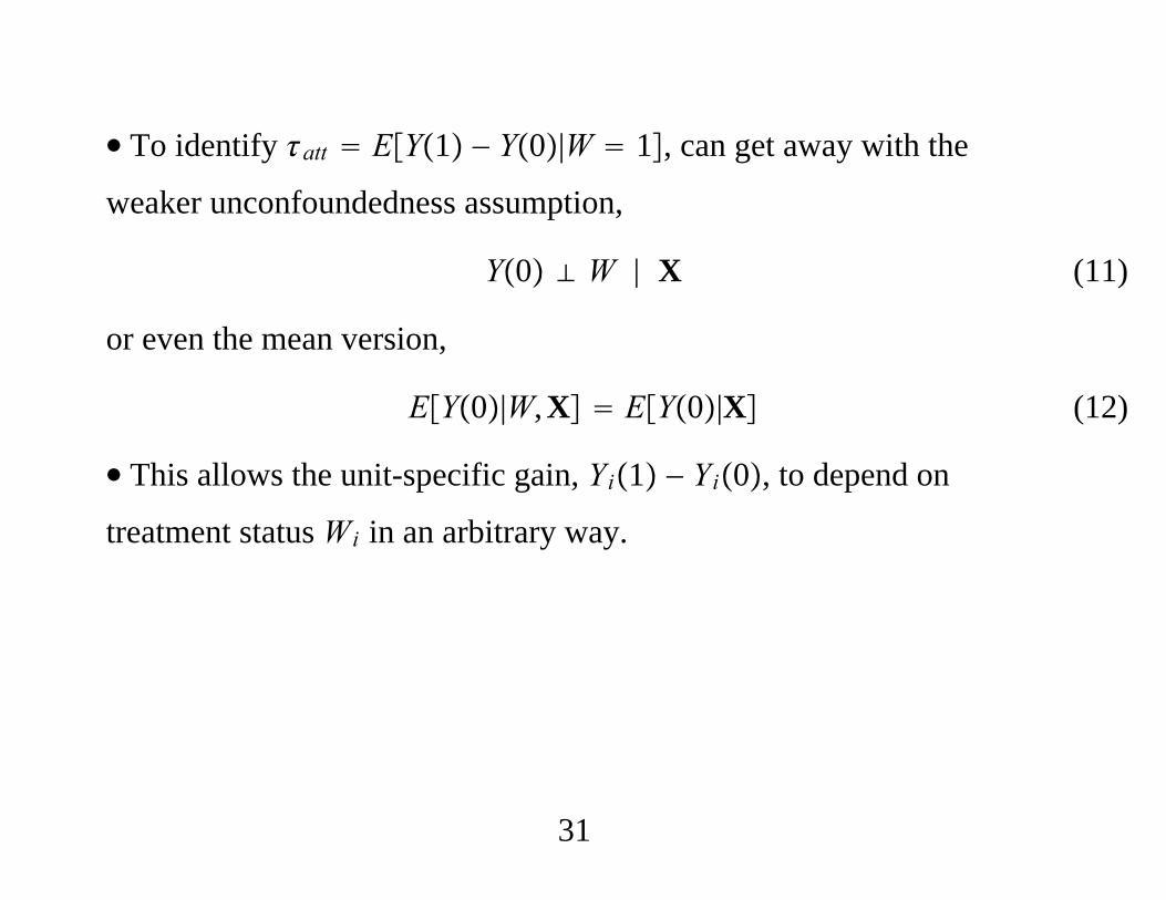
∙ To identify att EY1 − Y0|W 1, can get away with the

weaker unconfoundedness assumption,

Y0 W ∣ X (11)

or even the mean version,

EY0|W,X EY0|X (12)

∙ This allows the unit-specific gain, Yi1 − Yi0, to depend on

treatment status Wi in an arbitrary way.

31

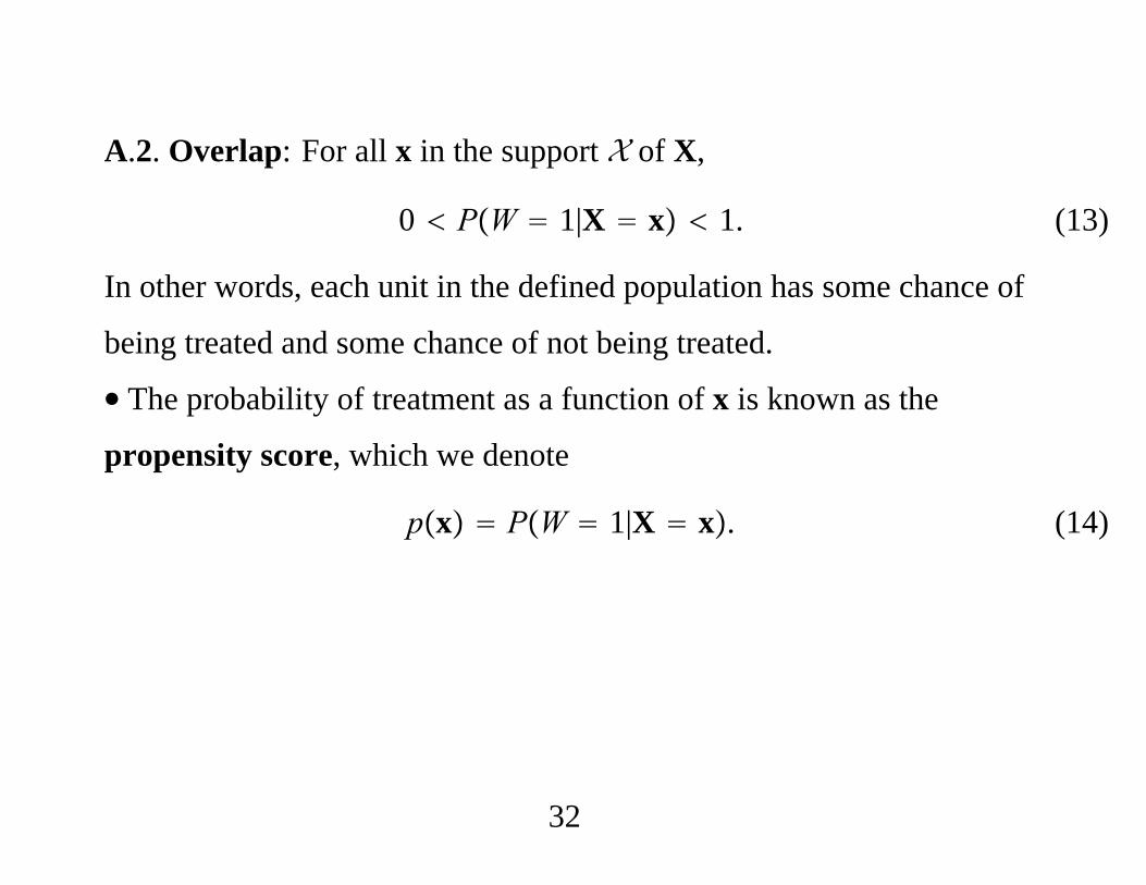
A.2. Overlap: For all x in the support X of X,

0 PW 1|X x 1. (13)

In other words, each unit in the defined population has some chance of

being treated and some chance of not being treated.

∙ The probability of treatment as a function of x is known as the

propensity score, which we denote

px PW 1|X x. (14)

32

∙ Strong Ignorability [Rosenbaum and Rubin (1983)]

Unconfoundedness plus Overlap.

∙ For ATT, overlap can be relaxed to

px 1 for all x ∈ X (15)

We can have px 0 because we average only over the treated

subpopulation.

33

4. Identification of Average Treatment Effects

∙ Two ways to show the treatment effects are identified under

unconfoundedness and overlap.

∙ First is based on regression functions. Define the average treatment

effect conditional on x as

x EY1 − Y0|X x 1x − 0x (16)

where gx ≡ EYg|X x, g 0, 1.

∙ The function x is of interest in its own right: it provides the

average treatment effect for different segments of the population

described by the observables, X.

34

∙ By iterated expectations, it is always true that

ate EY1 − Y0 EX E1X − 0X (17)

∙ It follows that ate is identified if 0 and 1 are identified over

the support (possibly values) of X, because we observe a random

sample on X and can average across its distribution.

35

∙ Define the conditional means of the observed outcome as

m0X EY|X,W 0,m1X EY|X,W 1 (19)

∙ Under overlap, m0 and m1 are nonparametrically identified on Xbecause we assume the availability of a random sample on Y,X,W.

∙When we add unconfoundedness we identify 0 and 1 because

EY|X,W 0 0X, EY|X,W 1 1X (20)

37

∙ In terms of the identified mean functions,

ate Em1X − m0Xatt Em1X − m0X|W 1

(22) (23)

∙ By definition we can always estimate Em1X|W 1, and so, for

att, we can get by with “partial” overlap. We need to be able to

estimate m0x for values of x taken on by the treatment group, which

translates into px 1 for all x ∈ X.

39

∙We can also establish identification of ate and att using the

propensity score. Assuming unconfoundedness, can show [Wooldridge

(2010, Chapter 21)]

E WYpX EY1

E 1 − WY1 − pX EY0

(24)

(25)

∙ Note where px 0 and px 1 come into play.

∙ Combining,

ate E WYpX −

1 − WY1 − pX E W − pXY

pX1 − pX . (26)

40

∙ Can also show

att EW − pXY1 − pX , (27)

where PW 1 is the unconditional probability of treatment.

∙ Only need px 1 because att is an average effect for those

eventually treated.

∙ The unconfoundedness and overlap assumptions to identify att are

weaker than for ate.

41

5. Estimating ATEs

∙When we assume unconfounded treatment and overlap, there are

three general approaches to estimating the treatment effects:

1. Regression-based methods (on covariates or propensity score).

2. Propensity score weighting methods.

3. Matching methods (on covariates or propensity score).

∙ Can mix the various approaches, and often this helps.

42

∙ Need to remember that all methods assume under unconfoundedness

and overlap. Even if unconfoundedness holds, they may behave quite

differently when overlap is weak.

∙ Under regularity conditions, asymptotically efficient estimators exist

under unconfoundedness and overlap. Using the propensity score in

regression or matching on are not efficient.

43

Regression Adjustment

∙ First step is to obtain m0x from the “control” subsample, Wi 0,

and m1x from the “treated” subsample, Wi 1. Can be as simple as

(flexible) linear regression or as complicated as full nonparametric

regression.

∙ Key: We compute a fitted value for each outcome for all units in

sample. For example, we only use the control units to obtain m0 but

we need m0Xi for the treated units, too.

44

∙ The regression-adjustment estimators are

ate,reg N−1∑i1

N

m1Xi − m0Xi

att,reg N1−1∑

i1

N

Wim1Xi − m0Xi

(28)

(29)

45

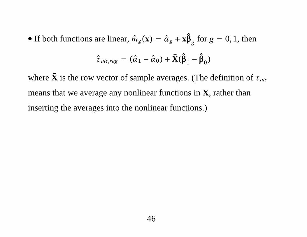
∙ If both functions are linear, mgx g xg for g 0, 1, then

ate,reg 1 − 0 X1 − 0

where X is the row vector of sample averages. (The definition of atemeans that we average any nonlinear functions in X, rather than

inserting the averages into the nonlinear functions.)

46

∙ Easiest way to obtain standard error for ate,reg is to ignore sampling

error in X and use the coefficient on Wi in the regression

Yi on 1, Wi, Xi, Wi Xi − X, i 1, . . . ,N. (30)

ate,reg is the coefficient on Wi.

47

∙ Important to demean Xi before forming interaction, so that the

coefficient on Wi is the estimate of ate.

∙ Centering the covariates before constructing the interactions is known

to often “solve” the multicollinearity problem in regression. It “solves”

the problem because it redefines the parameter we are trying to estimate

to be the ATE.

48

∙With lots of covariates, might compute differences in fitted values,

and average.

∙ In Stata:

reg y x1 x2 ... xK if ~treat

predict y0hat

reg y x1 x2 ... xK if treat

predict y1hat

gen ate_i y1hat - y0hat

sum ate_i

49

∙ The linear regression estimate of att is

att,reg 1 − 0 X11 − 0

where X1 is the average of the Xi over the treated subsample. It can be

obtained from

Yi on 1, Wi, Xi, Wi Xi − X1, i 1, . . . ,N. (31)

∙ Or, just average the difference in fitted values over the treated

subsample:

sum ate_i if treat

50

∙ If linear models do not seem appropriate for EY0|X and EY1|X,

the specific nature of the Yg can be exploited.

∙ If Y is a binary response, or a fractional response, estimate logit or

probit separately for the Wi 0 and Wi 1 subsamples and average

differences in predicted values:

ate,reg N−1∑i1

N

G1 Xi1 − G0 Xi0. (32)

∙ Each summand is the difference in estimate probabilities under

treatment and nontreatment for unit i, and the ATE just averages those

differences.

51

∙ In Stata (for binary or fractional response):

glm y x1 x2 ... xK if ~treat, fam(bin)

link(logit)

predict y0hat

glm y x1 x2 ... xK if treat, fam(bin)

link(logit)

predict y1hat

gen atei y1hat - y0hat

sum atei

52

∙ For general Y ≥ 0, Poisson regression with exponential mean is

attractive:

ate,reg N−1∑i1

N

exp1 Xi1 − exp0 Xi0. (33)

∙ In previous glm commands, substitute

fam(poisson) link(log)

∙ In nonlinear cases, can use delta method or bootstrap for standard

error of ate,reg. The delta method formula can be found in Wooldridge

(2010, Chapter 21).

53

∙Without good overlap in the covariate distribution, we must

extrapolate a parametric model – linear or nonlinear – into regions

where we do not have much or any data.

∙ For example, suppose only large firms offer equity incentives.

Estimating models of accounting irregularities will run into trouble if

firm size is in X. We have to estimate EY|X,W 1 using only firms

with equity incentives and then extrapolate the mean function to firms

not offering incentives.

54

∙ Nonparametric methods – see Imbens and Wooldridge (2009, Journal

of Economic Literature) are not helpful in overcoming poor overlap. If

they are global “series” estimators based on flexible parametric models,

they require extrapolation.

∙With local estimation methods (“kernel smoothing”), we cannot

easily estimate m1x for x values far away from those in the treated

subsample; similarly for m0x.

∙ Using local methods the problem of overlap is more obvious: we have

little or even no data to estimate the regression functions for values of x

with poor overlap.

55

∙ Using att has advantages because it requires only one extrapolation:

att,reg N1−1∑

i1

N

Wim1Xi − m0Xi. (34)

∙We only need to estimate m1x for values of x taken on by the

treated group, which we can do well. We do not need to estimate m1x

for values of x in the control group.

∙We still need to estimate m0x for the treated group.

56

Propensity Score Weighting

∙ The propensity score formula that establishes identification of atesuggests an estimator of ate:

ate,psw N−1∑i1

NWiYipXi

− 1 − WiYi1 − pXi

.

∙ ate,psw is not feasible because it depends on the unknown propensity

score p.

∙ Interestingly, we would not use it if we could! Even if we know p,

ate,psw is not asymptotically efficient. It is better to estimate the

propensity score!

57

∙ Two approaches: (1) Model p parametrically, in a flexible way

(probit or logit). Can show estimating the propensity score leads to a

smaller asymptotic variance when the parametric model is correctly

specified. (2) Use an explicit nonparametric approach, as in Hirano,

Imbens, and Ridder (2003, Econometrica) or Li, Racine, and

Wooldridge (2009, JBES).

58

ate,psw N−1∑i1

NWi − pXiYipXi1 − pXi

att,psw N−1∑i1

NWi − pXiYi1 − pXi

(35)

(36)

where N1/N is the fraction of treated in the sample.

59

∙ Clear that ate,psw can be sensitive to the choice of model for p

because now tail behavior can matter when px is close to zero or one.

(For att, only px close to unity matters.)

∙ These formulas show why trimming observations based on the PS is

often used.

60

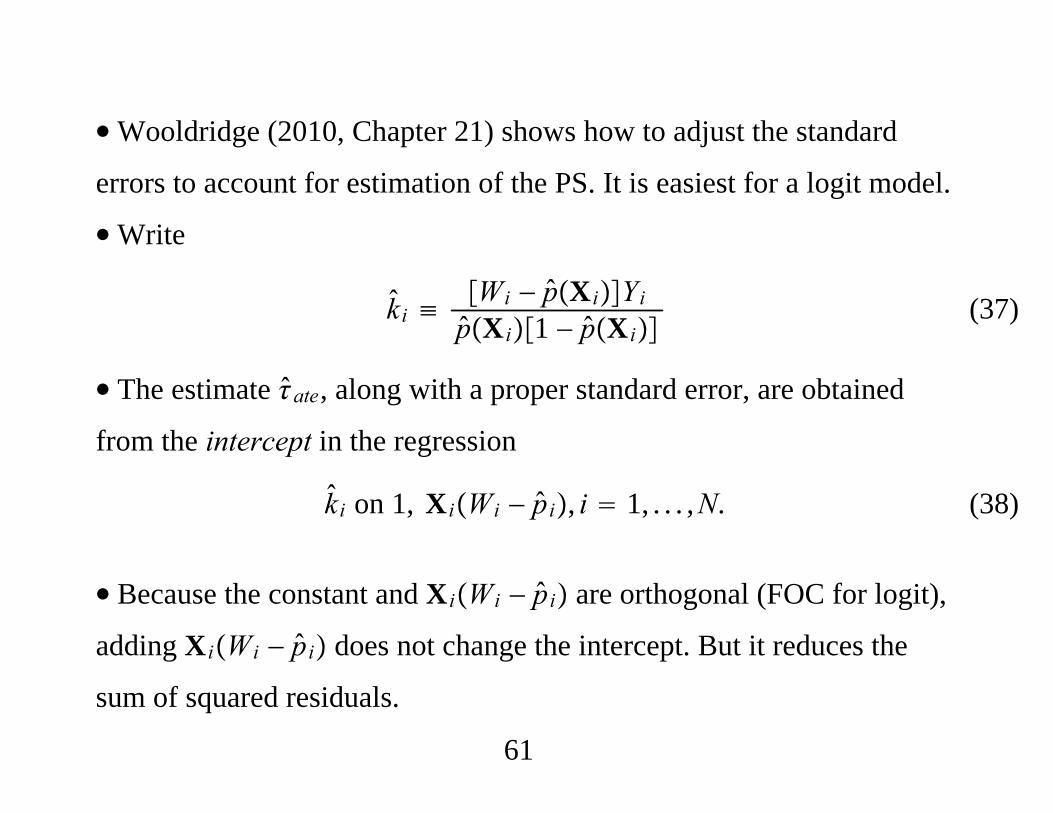
∙Wooldridge (2010, Chapter 21) shows how to adjust the standard

errors to account for estimation of the PS. It is easiest for a logit model.

∙Write

ki ≡Wi − pXiYipXi1 − pXi

(37)

∙ The estimate ate, along with a proper standard error, are obtained

from the intercept in the regression

ki on 1, XiWi − pi, i 1, . . . ,N. (38)

∙ Because the constant and XiWi − pi are orthogonal (FOC for logit),

adding XiWi − pi does not change the intercept. But it reduces the

sum of squared residuals.

61

∙ Also shows a result known in biostatistics: Asymptotically, we do no

worse – and typically better – by adding covariates to the logit

estimation even if they do not predict treatment!

62

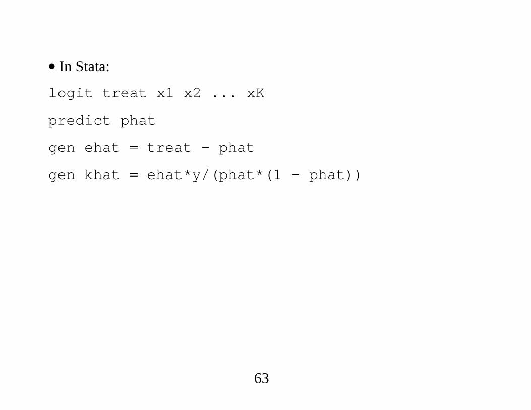
∙ In Stata:

logit treat x1 x2 ... xK

predict phat

gen ehat treat - phat

gen khat ehat*y/(phat*(1 - phat))

63

gen x1eh x1*eh

gen x2eh x2*eh

gen xKeh xK*eh

reg khat eh x1eh x2eh ... xKeh

∙ Obtain estimate and standard error as coefficient and standard error

on intercept.

64

∙ An alternative is to use bootstrapping, where the propensity score

estimation and averaging (to get ate,psw) are included in each bootstrap

iteration. Practical problem: Some bootstrap samples may give fitted

probabilities that are zero or one.

65

∙ Conservative to ignore the estimation error in the ki and simply treat

it as a random sample. That corresponds to just running the regression

ki on 1, i 1, . . . ,N.

∙ For att,psw, adjustment to standard error somewhat different

(Wooldridge, 2010, Chapter 21). Bootstrapping still can be used.

66

∙ Can see directly from ate,psw and att,psw that the inverse probability

weighted (IPW) estimators can be sensitive to extreme values of pXi.

att,psw is sensitive only to pXi ≈ 1, but ate,psw is also sensitive to

pXi ≈ 0.

∙ Imbens and coauthors have provided a rule-of-thumb: only use

observations with . 1 ≤ pXi ≤. 9 (for ATE). Drop observations and

start again on new, smaller sample.

∙ Sometimes the problem is pXi “close” to zero for many units,

which suggests the original population was not carefully chosen.

67

Regression on the Propensity Score

∙ Key result of Rosenbaum and Rubin (1983): Given

unconfoundedness conditional on X, unconfoundedness holds if we

condition only on pX:

Y0,Y1 W ∣ pX

and so

EY|pX,W 0 EY0|pXEY|pX,W 1 EY1|pX

68

∙ After estimating p by logit or probit, we estimate EY|pX,W 0

and EY|pX,W 1 using each subsample. For ate, use the average

difference in fitted values, as before.

∙ In the linear case, can obtain ate as the coefficient on Wi from the

pooled regression

Yi on 1, Wi, pXi, Wi pXi − p, i 1, . . . ,N (39)

where p N−1∑i1N pXi.

∙ The inference ignoring estimation of p is conservative. Can use the

bootstrap to obtain the smaller (valid) standard errors.

69

∙ Linear regression estimates such as (35) should not be too sensitive to

pi close to zero or one, but that might only mask the problem of poor

covariate balance.

∙ For a better fit, might use functions of the log-odds ratio,

ri ≡ log pXi1 − pXi

, (40)

as regressors when Y has a wide range. So, regress Yi on 1, ri, ri2, . . . , riQ

for some Q using both the control and treated samples, and then

average the difference in fitted values to obtain ate,regprop.

70

∙ Theoretically, regression on the propensity score in regression has

little to offer compared with other methods. It is not asymptotically

efficient.

71

Combining Regression Adjustment and PS Weighting

∙ Question: Why use regression adjustment combined with PS

weighting?

∙ Answer: With X having large dimension, still common to rely on

parametric methods for regression and PS estimation. Might worry

about misspecification.

72

∙ Idea: Let m0,0 and m1,1 be parametric functions for

EYg|X,g 0, 1. Let p, be a parametric model for the propensity

score. In the first step we estimate by logit or probit and obtain the

estimated propensity scores as pXi, .

73

∙ In the second step, we use regression or a quasi-likelihood method,

where we weight by the inverse probability.

∙ If the conditional means are linear, solve the WLS problem

min1,1∑i1

N

WiYi − 1 − Xi12/pXi, ; (41)

for 0, we weight by 1/1 − pXi and use the Wi 0 sample.

74

∙ ATE is estimated exactly as in the regression adjustment case, but

with different estimates of g,g:

ate,pswreg N−1∑i1

N

1 Xi1 − 0 Xi0. (42)

∙ Scharfstein, Rotnitzky, and Robins (1999, JASA) showed that

ate,psreg has a “double robustness” property: only one of the models

[mean or propensity score] needs to be correctly specified provided the

the mean and objective function are properly chosen [see also

Wooldridge (2007, Journal of Econometrics)].

75

∙ Y continuous, negative and positive values: linear mean, least squares

objective function, as above.

∙ Y binary or fractional: logit mean (not probit!), Bernoulli quasi-log

likelihood:

min1,1∑i1

N

Wi1 − Yi log1 − 1 Xi1

Yi log1 Xi1/pXi, .

(43)

76

∙ That is, probably use logit for Wi and Yi (for each subset, Wi 0 and

Wi 1).

∙ The ATE is estimated as before:

ate,pswreg N−1∑i1

N

1 Xi1 − 0 Xi0. (44)

77

∙ Sample Stata commands:

logit treat x1 x2 ... xK

predict phat

gen wght0 1/(1 - phat) if ~treat

gen wght1 1/phat if treat

78

∙ Linear Model:

reg y x1 x2 ... xK [pweight wght0] if ~treat

predict yh0

reg y x1 x2 ... xK [pweight wght1] if treat

predict yh1

gen ate_i yh1 - yh0

sum ate_i

∙ For standard error, can bootstrap.

79

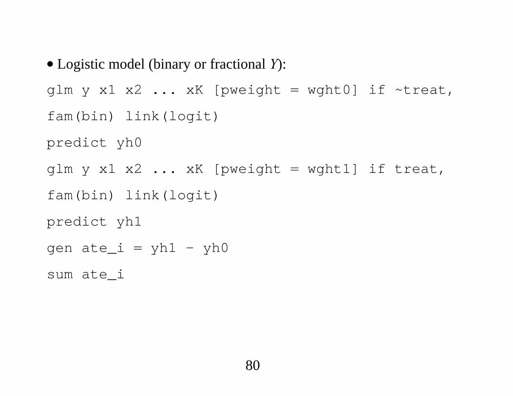
∙ Logistic model (binary or fractional Y):

glm y x1 x2 ... xK [pweight wght0] if ~treat,

fam(bin) link(logit)

predict yh0

glm y x1 x2 ... xK [pweight wght1] if treat,


predict yh1

gen ate_i yh1 - yh0

sum ate_i

80

∙ Y nonnegative, including count, continuous, or corners at zero:

exponential mean, Poisson quasi-MLE:

fam(poisson) link(log)

∙ In each case, must include a constant in the index models for

EY|W,X – the default.

∙ Rather than bootstrap, Stata module called dr can be used.

dr y treat, ovars(x1 ... xK) pvars(x1 ... xK)

dr y treat, ovars(x1 ... xK) pvars(x1 ... xK)


81

Matching

∙ Can match on a set of covariates or estimated propensity scores.

Matching on a large set of covariates can be very computationally

intensive.

∙Matching estimators are based on imputing a value on the

counterfactual outcome for each unit. That is, for a unit i in the control

group, we observe Yi0, but we need to impute Yi1. For each unit i in

the treatment group, we observe Yi1 but need to impute Yi0.

82

∙ For ate, matching estimators take the general form

ate,match N−1∑i1

N

Ŷi1 − Ŷi0 (45)

∙ Looks like regression adjustment except the imputed values are not

fitted values from regression. If we observe Yi1 then we use it, and

same for Yi0.

83

∙ For att,

att,match N1−1∑

i1

N

WiYi − Ŷi0, (46)

where this expression uses the fact that Yi Yi1 for the treated

subsample, and so we never have to impute Yi1.

84

∙ For covariate matching, Abadie and Imbens (2006, Econometrica)

consider several approaches. Simplest is to find a single match for each

observation. Suppose i is a treated observation (Wi 1). Then

Ŷi1 YiŶi0 Yh for h such that Wh 0

and unit h is “closest” to unit i based on some metric (distance) in the

covariates.

∙ For a treated unit i we find the “most similar” control observation,

and use its response as Yi0.

∙ If Wi 0, Ŷi0 Yi and Ŷi1 Yh where now Wh 1 and Xh is

“closest” to Xi.

85

∙ Abadie and Imbens matching has been programmed in Stata in the

command nnmatch. The default is to use the single nearest neighbor.

∙ The default matrix in defining distance is the inverse of the diagonal

matrix with sample variances of the covariates on the diagonal.

(Diagonal Mahalanobis.)

∙With a single variable to match on, the distance is just absolute value.

nnmatch y treat x1 x2 ... xK, tc(ate)

nnmatch y treat x1 x2 ... xK, tc(att)

86

∙We can impute the missing values using an average of M nearest

neighbors, or using all units h within a certain distance i – so-called

“caliper matching.”

∙ By choosing a distance and at most one match, can get no matches for

some units.

∙ Variance estimation of matching estimators is tricky. It is easiest to

use a conditional variance formula – programmed in nnmatch – but

this changes the “parameter” of interest to sate.

∙ Estimating the asymptotic variance when the parameter is ate is hard

due to a conditional bias.

87

Matching with Regression Adjustment

∙ The matching estimators have a large-sample bias if Xi has

dimension greater than one, on the order of N−1/K where K is the

number of covariates. Bias dominates the variance asymptotically when

K ≥ 3.

∙ The bias of the matching estimator comes from terms of the form

mwXhi − mwXi where mwx EY|X,W w.

88

∙ Let w be estimators – probably nonparametric – of the conditional

means. Define new imputations as

Yi1 Yi if Wi 1Yi1 Yhi m1Xi − m1Xhi if Wi 0Yi0 Yi if Wi 0Yi0 Yhi m0Xi − m0Xhi if Wi 1

89

∙ The bias-corrected matching estimator is

ate,bcme N−1∑i1

N

Yi1 − Yi0 (47)

∙ The BCME has the same (asymptotic) sampling variance as the

matching estimator, but the bias has been removed from the asymptotic

distribution [provided mw are sufficiently smooth].

∙ The nnmatch command in Stata allows for bias adjustment.

90

nnmatch y treat x1 x2 ... xK, tc(ate)

biasadj(bias)

∙ Unless one has strong priors, include the same covariates in

propensity score and regression models. (This is imposed by

nnmatch.) Exclusion restrictions do not help with unconfoundedness,

and they can hurt.

91

Matching on the Propensity Score

∙Matching on a full set of covariates can be computationally

demanding. Instead, can match on the estimated propensity score – a

single variable with range in 0, 1.

∙ The Stata command is psmatch2, and it allows a variety of options.

(For example, whether to estimate ATT or ATE, how many matches to

use, whether to use smoothing.)

∙ Until recently, valid inference not available for unsmoothed PS

matching unless we know the propensity score. Bootstrapping not

justified, but this is how Stata currently computes the standard errors.

92

∙ Abadie and Imbens (2011, unpublished, “Matching on the Estimated

Propensity Score”): Using matching with replacement, it is possible to

estimate the sampling variance of the PS matching estimator.

∙ Useful conclusion: The estimator that ignores estimation of the PS

turns out to be conservative. So can apply nnmatch with an estimated

propensity score to obain conservative inference.

93

6. Panel Data

∙ Lots of accounting applications with panel data. Several issues to

address.

1. How are average treatment effects defined with panel data and an

arbitrary pattern of treatments? Might there be persistent effects?

Simpler to assume there are only static effects or that only those effects

are of interest.

2. What covariates should be conditioned on? Many applications appear

to ignore lagged outcomes in covariates. Can use all information in a

sequential approach.

94

3. In matching approaches, should the matches be restricted? Without

restrictions, can match two firms in the same time period, two firms in

different time periods, or the same firm across different time periods.

∙ If matching is unrestricted, need the covariates to satisfy a “strict

exogeneity” assumption. Then matching should be based on entire

history of covariates or functions of them.

∙ In a pooled matching strategy, using lags of covariates does not solve

lack of strict exogeneity. Covariates that are affect by past shocks

cannot be conditioned on.

95

∙ A fixed effects approach effectively restricts matches to within a firm.

Think of T 2. FE is the same as differencing, and units without a

change in treatment status do not affect estimation.

∙ Fixed effects estimation can be derived from a counterfactual

framework where unconfoundedness holds conditional on unobserved

heterogeneity and the history of covariates.

∙ Allowing within-firm matching similar to fixed effects for firms that

switch: match is very likely to be within a firm over time.

96

∙ For firms with the same treatment status over time, how believable is

matching (and the overlap assumption)? We cannot allow matching on

an unobserved firm effect.

4. Statistical inference: How do we adjust usual statistics for time series

dependence in the panel data? Difficult with matching. Use “cluster

robust” options with regression or PS weighting.

∙When a panel is treated as a long cross section with unrestricted

matching, the usual bootstrap is incorrect: it ignores dependence across

time. Need panel bootstrap (resampling all time periods for each i).

97

∙ Sometimes see PS matching done based only on first-period

variables. Avoid this. Much less convincing than a fixed effects

analysis – which allows unobserved time-constant covariates – or a

sequential analysis that allows the propensity score to depend on the

recent past.

98

∙ Defining and estimating general “dynamic treatment effects” is

notationally hard; Wooldridge (2010, Chapter) contains a brief

treatment with references.

∙ A sequential setup, where at time t the counterfactual outcomes are

Yt0,Yt1, is easier.

99

∙ Two approaches. First, assume unconfoundedness of the entire

sequence of treatments, Wit : t 1, . . . ,, conditional on unobserved

heterogeneity, say ci, and a history of covariates, Xit : t 1, . . . ,T:

EYit0|Wi,Xi,ci EYit0|Xi,ciEYit1|Wi,Xi,ci EYit1|Xi,ci,

where Wi Wi1, . . . ,WiT is the time series of all treatments.

∙ Xit cannot include factors that react to shocks to previous outcomes

(so no lagged outcomes).

100

∙ Suppose

EYit0|Xi,ci t0 Xit0 ci0, (48)

and the expected gain from treatment is a function of Xit:

EYit1|Xi,ci EYit0|Xi,ci t Xit1. (49)

101

∙ Since Yit 1 − WitYit0 WitYit1,

EYit|Wi,Xi,ci t0 tWit Xit0 Wit Xit − t ci0 (50)

where t EXit.

∙ Estimation is by fixed effects (to remove ci0) including also time

dummies, and interacting the treatment with Xit − Xt.

∙ Setting 0 and t gives a standard fixed effects estimator of

ate.

102

∙ A second approach uses unconfoundedness conditional on past

observables.

∙ Let Xit denote a set of covariates observed prior to time t, including

past outcomes Yi,t−1, . . . ,Yi1 and and past treatments Wi,t−1, . . . ,Wi1.

Assume unconfoundedness conditional on Xit:

DWit|Yit0,Yit1,Xit DWit|Xi

t (51)

∙ Under this assumption, we can, at each time period t, apply regression

adjustment, propensity score weighting, or matching to obtain ate,t.

∙Might feel more comfortable using larger t that there is more to put in

Xit.

103

∙ There is a tradeoff between unconfoundedness and overlap. More in

Xit is better for unconfoundedness, worse for overlap. The effective

population may have to be reduced.

∙ For example, if we observe Wi1 Wi2 . . . Wi,t−1 1,

PWit 1|Xit may be very close to one.

104

∙ Using either approach, can get an overall average effect:

ate T−1∑t1

T

ate,t (52)

∙ Getting an appropriate standard error requires accounting for the

correlations in the estimators across time. Can use a “panel bootstrap,”

where cross-sectional units are resampled.

105

∙ Neither of the previous two approaches is more general than the

other: one is based on unobserved heterogeneity (a “firm fixed effect”),

the other on past observables.

∙ Both are preferred to the common practice of excluding past

responses and treatments in Xit and also ignoring unobserved firm

heterogeneity.

106

7. Application to Effects of Using a Big 4 Auditing Firm

∙ Subset of the data from Lawrence, Minutti-Meza, and Zhang (2011,

The Accounting Review).

∙ LMZ_cross.dta is a small cross-sectional data set for 2006.

LMZ_panel is a panel from 2001-2006, with values from 2000 as

controls.

∙ Use same SICs as LMZ.

∙ Treatment variable is big4, an indicator for using a Big 4 auditing

firm.

∙Main outcome is ada, absolute discretionary accurals.

107

∙ Covariates include total assets, total market value, return on assets,

measures of debts and liabilities. Also, industry and year dummies.

∙ LMZ pool data and treat a firm/year as the unit of observation.

Inference probably wrong. They do not use firm fixed effects or fully

dynamic matching.

108

. use LMZ_cross

. tab big4

big4 | Freq. Percent Cum.-----------------------------------------------

0 | 1,015 26.77 26.771 | 2,777 73.23 100.00

-----------------------------------------------Total | 3,792 100.00

. sum ada

Variable | Obs Mean Std. Dev. Min Max---------------------------------------------------------------------

ada | 3792 .1005575 .1452539 0 2.229223

109

. reg ada big4, robust

Linear regression Number of obs 3792F( 1, 3790) 65.43Prob F 0.0000R-squared 0.0274Root MSE .14327

------------------------------------------------------------------------------| Robust

ada | Coef. Std. Err. t P|t| [95% Conf. Interval]-----------------------------------------------------------------------------

big4 | -.054318 .0067149 -8.09 0.000 -.0674831 -.0411528_cons | .1403362 .0063556 22.08 0.000 .1278755 .1527969

------------------------------------------------------------------------------

. * Add lags of ada, big4:

. reg ada big4 ada_1 big4_1, robust

Linear regression Number of obs 3535F( 3, 3531) 29.79Prob F 0.0000R-squared 0.1403Root MSE .13359

------------------------------------------------------------------------------| Robust


big4 | -.0281794 .0112102 -2.51 0.012 -.0501584 -.0062004ada_1 | .3914005 .0554027 7.06 0.000 .282776 .5000251

big4_1 | -.0113145 .0117728 -0.96 0.337 -.0343966 .0117676_cons | .0931548 .0066316 14.05 0.000 .0801527 .1061569

------------------------------------------------------------------------------

110

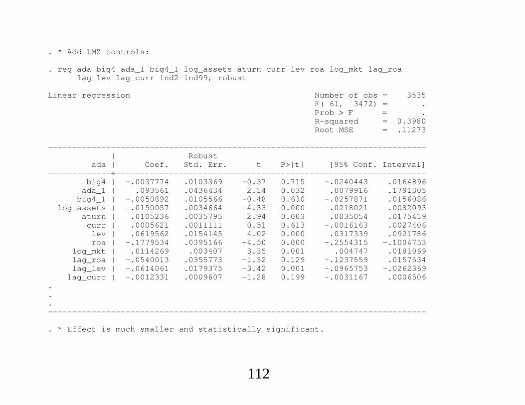
. * Add LMZ controls:

. reg ada big4 ada_1 big4_1 log_assets aturn curr lev roa log_mkt lag_roalag_lev lag_curr ind2-ind99, robust

Linear regression Number of obs 3535F( 61, 3472) .Prob F .R-squared 0.3980Root MSE .11273

------------------------------------------------------------------------------| Robust


big4 | -.0037774 .0103369 -0.37 0.715 -.0240443 .0164896ada_1 | .093561 .0436434 2.14 0.032 .0079916 .1791305

big4_1 | -.0050892 .0105566 -0.48 0.630 -.0257871 .0156086log_assets | -.0150057 .0034664 -4.33 0.000 -.0218021 -.0082093

aturn | .0105236 .0035795 2.94 0.003 .0035054 .0175419curr | .0005621 .0011111 0.51 0.613 -.0016163 .0027406

lev | .0619562 .0154145 4.02 0.000 .0317339 .0921786roa | -.1779534 .0395166 -4.50 0.000 -.2554315 -.1004753

log_mkt | .0114269 .003407 3.35 0.001 .004747 .0181069lag_roa | -.0540013 .0355773 -1.52 0.129 -.1237559 .0157534lag_lev | -.0614061 .0179375 -3.42 0.001 -.0965753 -.0262369

lag_curr | -.0012331 .0009607 -1.28 0.199 -.0031167 .0006506...------------------------------------------------------------------------------

. * Effect is much smaller and statistically significant.

112

. * Now use separate linear regressions:

. * clear all

.

. capture program drop ateboot

.

. program ateboot, eclass1.

. * Estimate linear model on each treatment group

. tempvar touse2. gen byte ‘touse’ 13. reg ada ada_1 big4_1 log_assets aturn curr lev roa log_mkt l

ag_roa lag_lev lag_curr ind2-ind99 if big44. predict adah15. reg ada ada_1 big4_1 log_assets aturn curr lev roa log_mkt

lag_roa lag_lev lag_curr ind2-ind99 if ~big46. predict adah07.

. gen ate_i adah1 - adah08. sum ate_i9. scalar ate r(mean)

10. sum ate_i if big411. scalar att r(mean)12.

. matrix b (ate, att)13. matrix colnames b ate att14.

. ereturn post b , esample(‘touse’)15. ereturn display16.

. drop adah1 adah0 ate_i17.

. end

114

.

. bootstrap _b[ate] _b[att], reps(1000) seed(123): ateboot(running ateboot on estimation sample)

Bootstrap replications (1000)------- 1 ------ 2 ------ 3 ------ 4 ------ 5.................................................. 50

.................................................. 1000

Bootstrap results Number of obs 3792Replications 1000

command: ateboot_bs_1: _b[ate]_bs_2: _b[att]

------------------------------------------------------------------------------| Observed Bootstrap Normal-based| Coef. Std. Err. z P|z| [95% Conf. Interval]

-----------------------------------------------------------------------------_bs_1 | -.002738 .0114702 -0.24 0.811 -.0252192 .0197431_bs_2 | .0003525 .0146904 0.02 0.981 -.0284401 .029145

------------------------------------------------------------------------------

.

. program drop ateboot

.end of do-file

. * To get regression adjustment, can use the double-robust approach

. * without any pvars:

. dr ada big4, ovars(ada_1 big4_1 log_assets aturn curr lev roa

115

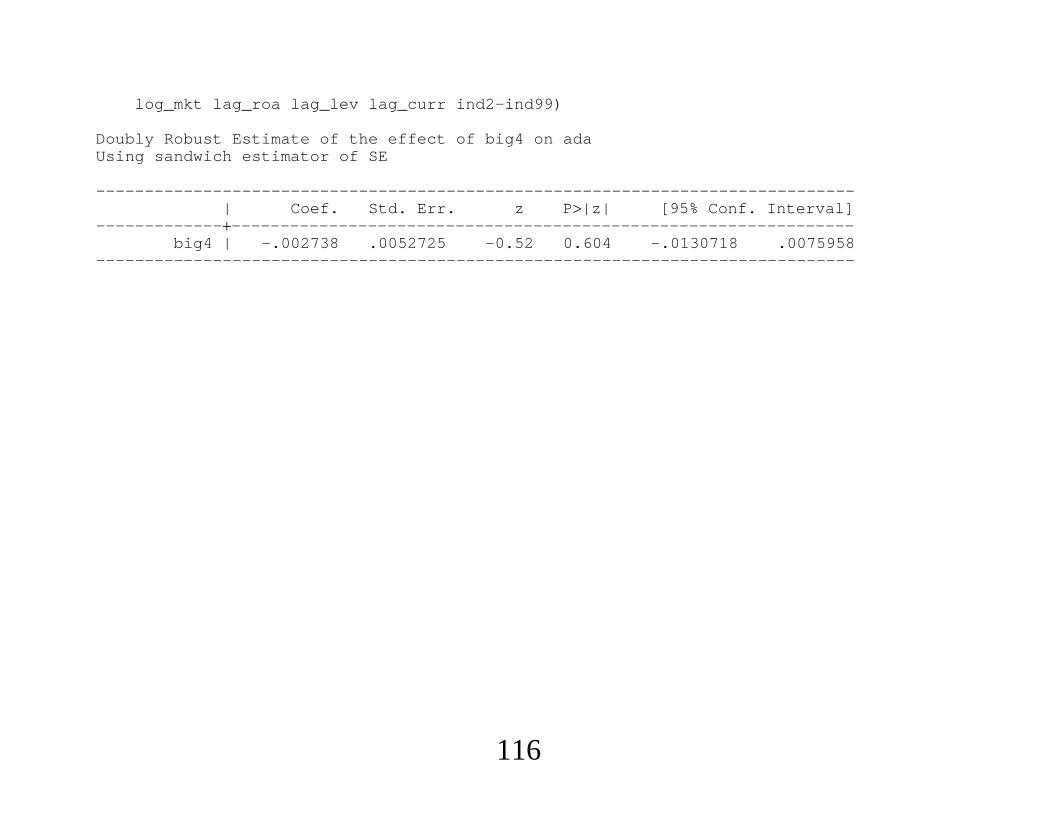
log_mkt lag_roa lag_lev lag_curr ind2-ind99)

Doubly Robust Estimate of the effect of big4 on adaUsing sandwich estimator of SE

------------------------------------------------------------------------------| Coef. Std. Err. z P|z| [95% Conf. Interval]

-----------------------------------------------------------------------------big4 | -.002738 .0052725 -0.52 0.604 -.0130718 .0075958

------------------------------------------------------------------------------

116

. * Now use PS matching. Use nnmatch to obtain conservative standard errors.

. * qui logit big4 ada_1 big4_1 log_assets aturn curr lev roa log_mktlag_roa lag_lev lag_curr ind2-ind99

. predict phat(option pr assumed; Pr(big4))(307 missing values generated)

. sum phat


phat | 3485 .7268293 .3969844 .0005813 .9997486

. * Overlap looks like it may be a problem.

. count if phat .05 | phat .952828

. sum phat if big4


phat | 2533 .9437114 .124395 .0036205 .9997486

. sum phat if ~big4


phat | 952 .1497679 .2784276 .0005813 .992681

117

. nnmatch ada big4 phat, tc(ate)307 observations dropped due to treatment variable missing

Matching estimator: Average Treatment Effect ate

Number of obs 3485Number of matches (m) 1

------------------------------------------------------------------------------ada | Coef. Std. Err. z P|z| [95% Conf. Interval]

-----------------------------------------------------------------------------SATE | .0109919 .029483 0.37 0.709 -.0467938 .0687776

------------------------------------------------------------------------------Matching variables: phat

. nnmatch ada big4 phat, tc(att)307 observations dropped due to treatment variable missing

Matching estimator: Average Treatment Effect for the Treated

Number of obs 3485Number of matches (m) 1

------------------------------------------------------------------------------ada | Coef. Std. Err. z P|z| [95% Conf. Interval]

-----------------------------------------------------------------------------SATT | .0237566 .0329039 0.72 0.470 -.0407339 .088247

------------------------------------------------------------------------------Matching variables: phat

119

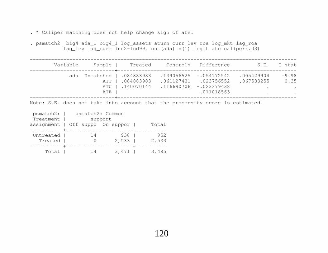
. * Caliper matching does not help change sign of ate:

. psmatch2 big4 ada_1 big4_1 log_assets aturn curr lev roa log_mkt lag_roalag_lev lag_curr ind2-ind99, out(ada) n(1) logit ate caliper(.03)

----------------------------------------------------------------------------------------Variable Sample | Treated Controls Difference S.E. T-stat

---------------------------------------------------------------------------------------ada Unmatched | .084883983 .139056525 -.054172542 .005429904 -9.98

ATT | .084883983 .061127431 .023756552 .067533255 0.35ATU | .140070144 .116690706 -.023379438 . .ATE | .011018563 . .

---------------------------------------------------------------------------------------Note: S.E. does not take into account that the propensity score is estimated.

psmatch2: | psmatch2: CommonTreatment | support

assignment | Off suppo On suppor | Total-------------------------------------------

Untreated | 14 938 | 952Treated | 0 2,533 | 2,533

-------------------------------------------Total | 14 3,471 | 3,485

120

. * Inverse PS weighting:

. gen kate_i (big4 - phat)*ada/(phat*(1 - phat))(307 missing values generated)

. reg kate_i

Source | SS df MS Number of obs 3485------------------------------------------- F( 0, 3484) 0.00

Model | 0 0 . Prob F .Residual | 6634.63194 3484 1.90431456 R-squared 0.0000

------------------------------------------- Adj R-squared 0.0000Total | 6634.63194 3484 1.90431456 Root MSE 1.38

------------------------------------------------------------------------------kate_i | Coef. Std. Err. t P|t| [95% Conf. Interval]

-----------------------------------------------------------------------------_cons | .0411547 .0233759 1.76 0.078 -.0046771 .0869865

------------------------------------------------------------------------------

. * Probably too dangerous because of very small and large probabilities.

. * Bootstrap gives many samples with perfect fits of the PS.

121

. * Now double robustness, first using linear model, then exponential:

. dr ada big4, ovars(ada_1 big4_1 log_assets aturn curr lev roa log_mktlag_roa lag_lev lag_curr ind2-ind99)pvars(ada_1 big4_1 log_assets aturn curr lev roa log_mkt lag_roalag_lev lag_curr ind2-ind99)



-----------------------------------------------------------------------------big4 | .0011662 .0126976 0.09 0.927 -.0237207 .0260531

------------------------------------------------------------------------------

. dr ada big4, ovars(ada_1 big4_1 log_assets aturn curr lev roa log_mktlag_roa lag_lev lag_curr ind2-ind99)

pvars(ada_1 big4_1 log_assets aturn curr lev roa log_mkt lag_roalag_lev lag_curr ind2-ind99) fam(poiss) link(log)



-----------------------------------------------------------------------------big4 | .011741 .0123333 0.95 0.341 -.0124319 .0359138

------------------------------------------------------------------------------

122

. * Now use firms with big4 0 in 2005:

. use LMZ_small

. do linreg_LMZ_small

. * clear all

.

. capture program drop ateboot

.

. program ateboot, eclass1.

. * Estimate linear model on each treatment group

. tempvar touse2. gen byte ‘touse’ 13. reg ada ada_1 log_assets aturn curr lev roa log_mkt

lag_roa lag_lev lag_curr ind2-ind99 if big44. predict adah15. reg ada ada_1 log_assets aturn curr lev roa log_mkt

lag_roa lag_lev lag_curr ind2-ind99 if ~big46. predict adah07.

. gen ate_i adah1 - adah08. sum ate_i9. scalar ate r(mean)

10. sum ate_i if big411. scalar att r(mean)12.

. matrix b (ate, att)13. matrix colnames b ate att14.

. ereturn post b , esample(‘touse’)15. ereturn display16.

. drop adah1 adah0 ate_i

124

17.. end

. bootstrap _b[ate] _b[att], reps(1000) seed(123): ateboot(running ateboot on estimation sample)

Bootstrap results Number of obs 862Replications 1000

command: ateboot_bs_1: _b[ate]_bs_2: _b[att]

------------------------------------------------------------------------------| Observed Bootstrap Normal-based| Coef. Std. Err. z P|z| [95% Conf. Interval]

-----------------------------------------------------------------------------_bs_1 | -.0607535 .1903262 -0.32 0.750 -.4337859 .312279_bs_2 | .0005891 .0193423 0.03 0.976 -.0373212 .0384994

------------------------------------------------------------------------------.. program drop ateboot

. dr ada big4, ovars(ada_1 log_assets aturn curr lev roa log_mkt lag_roalag_lev lag_curr ind2-ind99) pvars(ada_1 big4_1 log_assetsaturn curr lev roa log_mkt lag_roa lag_lev lag_curr ind2-ind99)



-----------------------------------------------------------------------------big4 | -.0242166 .0249231 -0.97 0.331 -.073065 .0246318

------------------------------------------------------------------------------

125

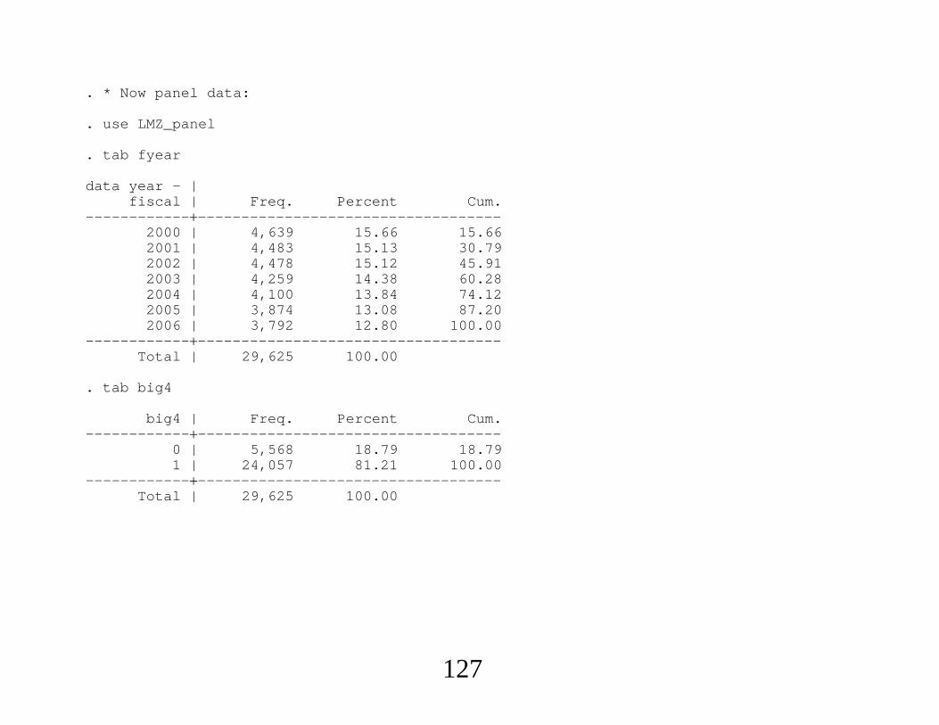
. * Now panel data:

. use LMZ_panel

. tab fyear

data year - |fiscal | Freq. Percent Cum.

-----------------------------------------------2000 | 4,639 15.66 15.662001 | 4,483 15.13 30.792002 | 4,478 15.12 45.912003 | 4,259 14.38 60.282004 | 4,100 13.84 74.122005 | 3,874 13.08 87.202006 | 3,792 12.80 100.00

-----------------------------------------------Total | 29,625 100.00

. tab big4

big4 | Freq. Percent Cum.-----------------------------------------------

0 | 5,568 18.79 18.791 | 24,057 81.21 100.00

-----------------------------------------------Total | 29,625 100.00

127

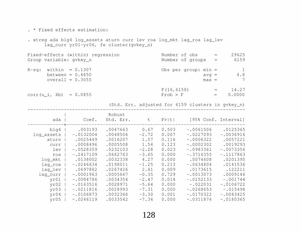
. * Fixed effects estimation:

. xtreg ada big4 log_assets aturn curr lev roa log_mkt lag_roa lag_levlag_curr yr01-yr06, fe cluster(gvkey_n)

Fixed-effects (within) regression Number of obs 29625Group variable: gvkey_n Number of groups 6159

R-sq: within 0.1307 Obs per group: min 1between 0.4850 avg 4.8overall 0.3055 max 7

F(16,6158) 14.27corr(u_i, Xb) 0.0855 Prob F 0.0000

(Std. Err. adjusted for 6159 clusters in gvkey_n)------------------------------------------------------------------------------

| Robustada | Coef. Std. Err. t P|t| [95% Conf. Interval]

-----------------------------------------------------------------------------big4 | .003193 .0047663 0.67 0.503 -.0061506 .0125365

log_assets | -.0132004 .0048506 -2.72 0.007 -.0227093 -.0036916aturn | .0025449 .0016207 1.57 0.116 -.0006322 .0057221

curr | .0008496 .0005508 1.54 0.123 -.0002302 .0019293lev | -.0528359 .0232103 -2.28 0.023 -.0983361 -.0073356roa | -.2417109 .0662763 -3.65 0.000 -.3716355 -.1117863

log_mkt | .0138002 .0032338 4.27 0.000 .0074608 .0201395lag_roa | -.0246634 .0198011 -1.25 0.213 -.0634804 .0141536lag_lev | .0697862 .0267426 2.61 0.009 .0173615 .122211

lag_curr | -.0001963 .0005667 -0.35 0.729 -.0013073 .0009146yr01 | -.0084786 .0034354 -2.47 0.014 -.0152133 -.001744yr02 | -.0163516 .0028971 -5.64 0.000 -.022031 -.0106722yr03 | -.0211816 .0028993 -7.31 0.000 -.0268653 -.015498yr04 | -.0106873 .0032366 -3.30 0.001 -.0170322 -.0043425yr05 | -.0246119 .0033542 -7.34 0.000 -.0311874 -.0180365

128

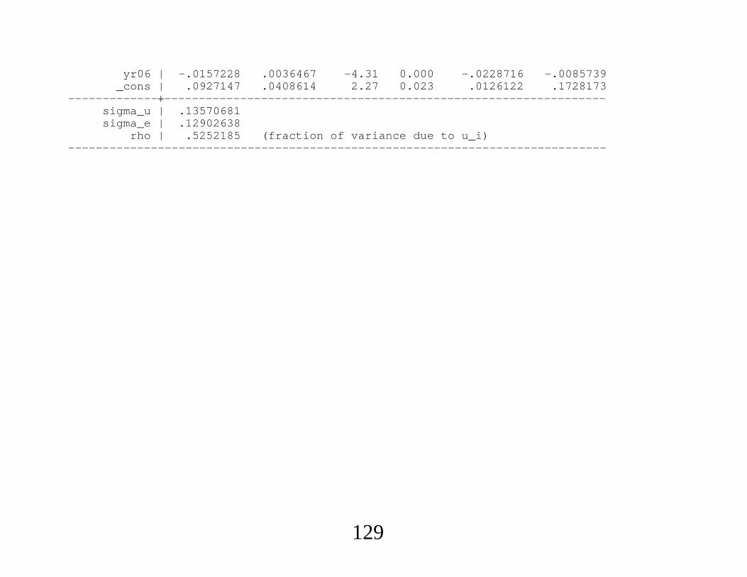
yr06 | -.0157228 .0036467 -4.31 0.000 -.0228716 -.0085739_cons | .0927147 .0408614 2.27 0.023 .0126122 .1728173

-----------------------------------------------------------------------------sigma_u | .13570681sigma_e | .12902638

rho | .5252185 (fraction of variance due to u_i)------------------------------------------------------------------------------

129

. * Pooled matching, as in LMZ. Standard errors incorrect because time series

. * correlation ignored. Also, estimated propensity score ignored:

. psmatch2 big4 log_assets aturn curr lev roa log_mkt lag_roa lag_levlag_curr yr01-yr06 ind2-ind99, out(ada) n(1) ate logit


---------------------------------------------------------------------------------------ada Unmatched | .099083692 .15591834 -.056834648 .002551798 -22.27

ATT | .099083692 .107141449 -.008057757 .01024832 -0.79ATU | .15591834 .14861206 -.00730628 . .ATE | -.007916044 . .

---------------------------------------------------------------------------------------

130

. * Sequential matching:

. psmatch2 big4 ada_1 big4_1 log_assets aturn curr lev roa log_mkt lag_roalag_lev lag_curr ind2-ind99 if yr01, out(ada) n(1) ate


---------------------------------------------------------------------------------------ada Unmatched | .111706441 .162546089 -.050839648 .006324887 -8.04

ATT | .111706441 .113419543 -.001713102 .066729983 -0.03ATU | .162546089 .171438524 .008892435 . .ATE | -.000166068 . .

---------------------------------------------------------------------------------------



---------------------------------------------------------------------------------------ada Unmatched | .098112904 .153769922 -.055657018 .006005934 -9.27

ATT | .098112904 .103298256 -.005185352 .044479146 -0.12ATU | .153769922 .149525088 -.004244833 . .ATE | -.005030568 . .

---------------------------------------------------------------------------------------



---------------------------------------------------------------------------------------ada Unmatched | .089687347 .150904827 -.06121748 .006238025 -9.81

ATT | .089687347 .112017109 -.022329762 .032756893 -0.68ATU | .150904827 .166038042 .015133216 . .ATE | -.015891694 . .

131

---------------------------------------------------------------------------------------



---------------------------------------------------------------------------------------ada Unmatched | .091364716 .172477806 -.081113091 .009079242 -8.93

ATT | .091364716 .099152418 -.007787702 .022627015 -0.34ATU | .172477806 .101160802 -.071317004 . .ATE | -.021035827 . .

---------------------------------------------------------------------------------------

. * Regression adjustment:

. dr ada big4 if yr04, ovars(ada_1 big4_1 log_assets aturn curr lev roa log_mktlag_roa lag_lev lag_curr ind2-ind99)



-----------------------------------------------------------------------------big4 | -.0100175 .0086784 -1.15 0.248 -.0270269 .0069919

------------------------------------------------------------------------------

. * PS weighting:

. dr ada big4 if yr04, pvars(ada_1 big4_1 log_assets aturn curr levroa log_mkt lag_roa lag_lev lag_curr ind2-ind99)

Doubly Robust Estimate of the effect of big4 on ada

132

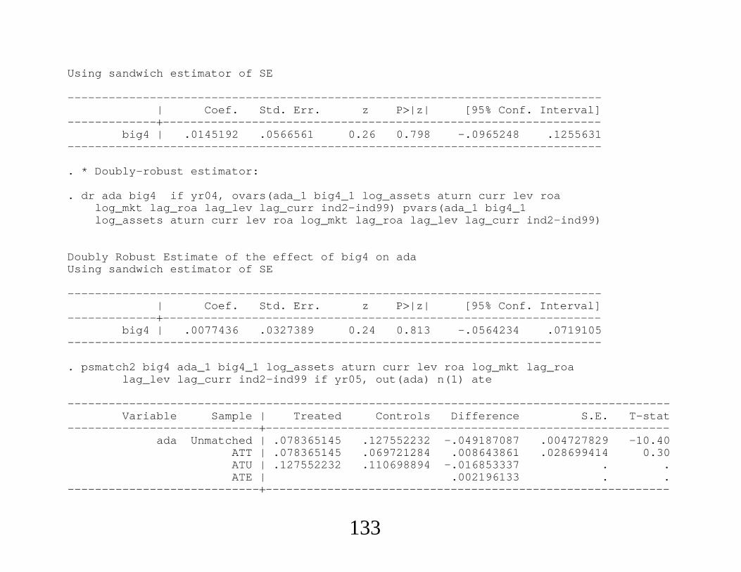
Using sandwich estimator of SE


-----------------------------------------------------------------------------big4 | .0145192 .0566561 0.26 0.798 -.0965248 .1255631

------------------------------------------------------------------------------

. * Doubly-robust estimator:

. dr ada big4 if yr04, ovars(ada_1 big4_1 log_assets aturn curr lev roalog_mkt lag_roa lag_lev lag_curr ind2-ind99) pvars(ada_1 big4_1log_assets aturn curr lev roa log_mkt lag_roa lag_lev lag_curr ind2-ind99)



-----------------------------------------------------------------------------big4 | .0077436 .0327389 0.24 0.813 -.0564234 .0719105

------------------------------------------------------------------------------



---------------------------------------------------------------------------------------ada Unmatched | .078365145 .127552232 -.049187087 .004727829 -10.40

ATT | .078365145 .069721284 .008643861 .028699414 0.30ATU | .127552232 .110698894 -.016853337 . .ATE | .002196133 . .

---------------------------------------------------------------------------------------

133



---------------------------------------------------------------------------------------ada Unmatched | .084883983 .139056525 -.054172542 .005429904 -9.98

ATT | .084883983 .068711041 .016172942 .051404095 0.31ATU | .139056525 .114961423 -.024095102 . .ATE | .005172891 . .

---------------------------------------------------------------------------------------Note: S.E. does not take into account that the propensity score is estimated.

134

8. Assessing Unconfoundedness

∙ Unconfoundedness is not directly testable. Any assessment is indirect.

∙ Several possibilities. Given several pre-treatment outcomes, can

construct a treatment effect on a pseudo outcome and establish that it is

not statistically different from zero.

∙ Suppose controls consist of time-constant characteristics, Zi, and

three pre-assignment outcomes on the response, Yi,−1,Yi,−2, and Yi,−3.

Let the counterfactual outcomes be at t 0, Yi00 and Yi01. Suppose

we are willing to assume unconfoundedness given two lags:

Yi00,Yi01 Wi ∣ Yi,−1,Yi,−2,Zi (53)

135

∙ If the process generating Yisg is appropriately stationary and

exchangeable, it can be shown that

Yi,−1 Wi,∣ Yi,−2,Yi,−3,Zi, (54)

and this is testable. Conditional on Yi,−2,Yi,−3,Zi, Yi,−1 should not

differ systematically for the treatment and control groups.

∙ Can regress Yi,−1 on Yi,−2, Yi,−3, Zi for Wi 0 and Wi 1 and

peform Chow test.

∙ Or, estimate logit or probit for PWi 1|Yi,−1,Yi,−2,Yi,−3,Zi and test

Yi,−1 for significance.

136

∙ Alternatively, can try to assess sensitivity to failure of

unconfoundedness by using a specific alternative mechanism. For

example, suppose unconfoundedness holds conditional on an

unobservable, V, in addition to X:

Yi0,Yi1 Wi ∣ Xi,Vi

If we parametrically specify EYig|Xi,Vi, g 0, 1, specify

PWi 1|Xi,Vi, assume (typically) that Vi and Xi are independent,

then ate can be obtained in terms of the parameters of all

specifications.

137

∙ In practice, we consider the version of ATE conditional on the

covariates in the sample, cate – the “conditional” ATE – so that we

only have to integrate out Vi. Often, Vi is assumed to be very simple,

such as a binary variable (indicating two “types”).

∙ Even for simple schemes, approach is complicated. One set of

parameters are “sensitivity” parameters, other set is estimated. Then,

evaluate how cate changes with the sensitivity parameters.

∙ See Imbens (2003) or Imbens and Wooldridge (2009) for details.

138

9. Assessing and Improving Overlap

∙ A simple step is to compute normalized differences for each

covariate. Let X1j and X0j be the means of covariate j for the treated and

control subsamples, respectively, and let S1j and S0j be the estimated

standard deviations. Then the normalized difference is

normdiffj X1j − X0j

S1j2 S0j

2 (55)

∙ Imbens and Rubin discuss a rule-of-thumb: Normalized differences

above about . 25 are cause for concern.

139

∙ normdiffj is not the t statistic for comparing the means of the

distribution. The t statistic depends explicitly on the sample sizes. Here

interested in difference in population distributions, not statistical

significance.

∙ Limitation of looking at the normalized differences: they only

consider each marginal distribution. There can still be areas of weak

overlap in the support X even if the normalized differences are all

similar.

140

∙ Easier to look directly at the propensity scores, or the log-odds of the

propensity score. In other words, compute the normalized difference of

a single “balancing” function of Xi.

∙ Also look directly at the histograms of estimated propensity scores for

the treated and control groups. The command psgraph does this after

using psmatch2.

141

∙ If there are problems with overlap in the original sample, may have to

redefine the population. [Focusing on att rather than ate can solve part

of the overlap problem because PW 1|X 0 is allowed for att.]

∙ Earlier mentioned the rule of dropping i if pXi ∉ . 1, . 9. Can lose

a lot of data, including treated observations. Resulting population might

not be what we want. Does not always solve the overlap problem.

142

∙ Or, use the estimated PS to match each treated unit with a single

control unit, to obtain a new sample with the same number of treated

and controls.

∙ After using all of the data to estimate the PS, for treated units order

from largest to smallest PS. Starting at top, match the first treated unit

to the closest control. Then do the same for the next treated unit (not

replacing the control units). If there are N1 treated units, we wind up

with N1 controls, too.

∙ The new smaller – in some cases, much smaller – sample is better

balanced. Can apply all the usual methods for ate.

143

∙ Has the advantage of keeping all treated observations. But the

population is hard to interpret.

∙Might be better to think about a sensible population ahead of time. If

a firm has used a Big Four accounting firm over all twelve years of a

sample, should it be included in a study of the effects of using one of

the Big Four? These firms would fall out of a fixed effects analysis.

144

. * With full cross section in 2006:

. pstest ada_1 big4_1 log_assets aturn curr lev roa log_mkt lag_roa lag_lev lag_curr

----------------------------------------------------------------------------| Mean %reduct | t-test

Variable Sample | Treated Control %bias |bias| | t p|t|--------------------------------------------------------------------------

ada_1 Unmatched | .07799 .12128 -31.1 | -9.23 0.000Matched | .07799 .05381 17.4 44.1 | 9.21 0.000

| |big4_1 Unmatched | .98381 .13866 324.7 | 105.72 0.000

Matched | .98381 .9846 -0.3 99.9 | -0.23 0.822| |

log_assets Unmatched | 6.8268 4.116 160.3 | 39.51 0.000Matched | 6.8268 6.4343 23.2 85.5 | 8.06 0.000

| |aturn Unmatched | 1.105 1.2815 -17.9 | -5.04 0.000

Matched | 1.105 .99216 11.5 36.0 | 5.26 0.000| |

curr Unmatched | 2.6542 3.3653 -21.2 | -5.89 0.000Matched | 2.6542 2.5049 4.4 79.0 | 2.16 0.031

| |lev Unmatched | .21688 .19255 5.4 | 1.76 0.079

Matched | .21688 .26278 -10.1 -88.6 | -6.76 0.000| |

roa Unmatched | .00105 -.11701 31.0 | 9.71 0.000Matched | .00105 .01105 -2.6 91.5 | -1.55 0.122

| |log_mkt Unmatched | 6.9848 4.4475 155.8 | 38.83 0.000

Matched | 6.9848 6.7165 16.5 89.4 | 5.67 0.000| |

lag_roa Unmatched | .00577 -.09574 33.5 | 10.37 0.000Matched | .00577 .03216 -8.7 74.0 | -5.38 0.000

| |

145

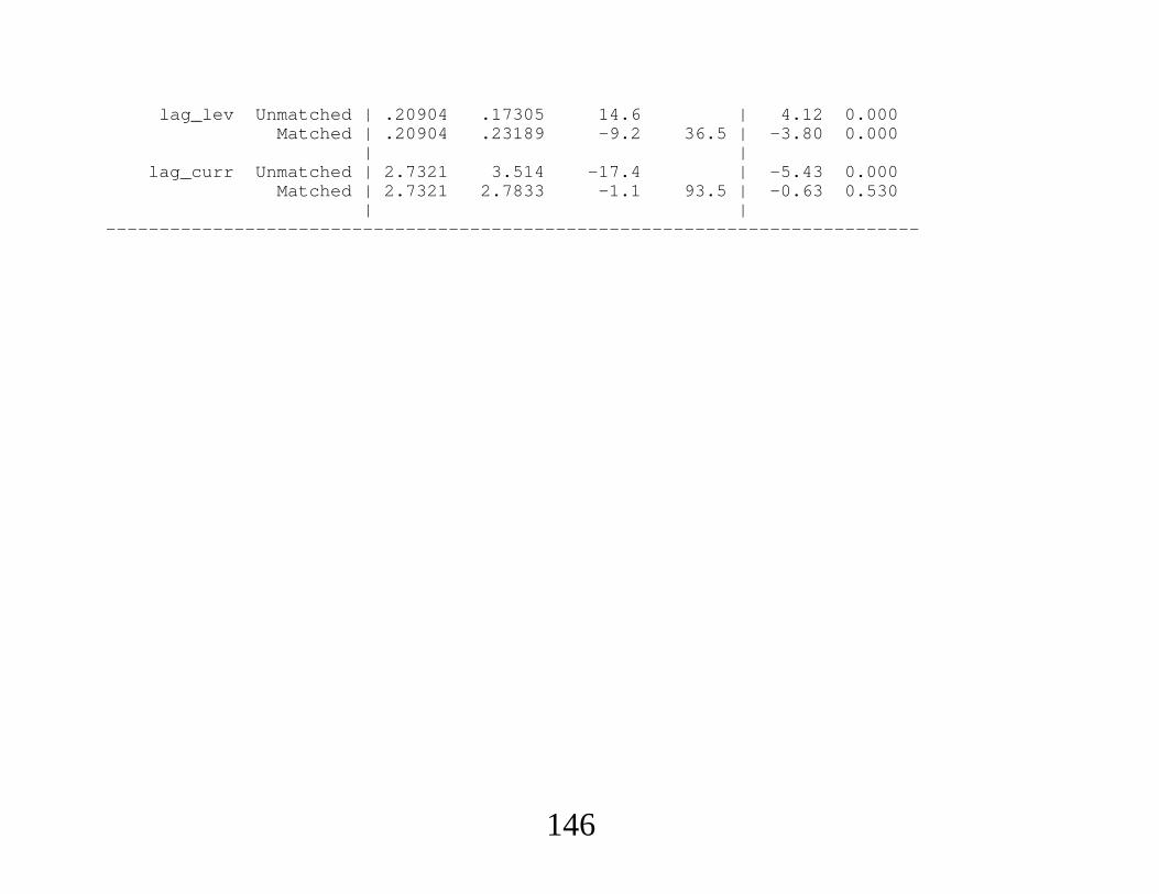
lag_lev Unmatched | .20904 .17305 14.6 | 4.12 0.000Matched | .20904 .23189 -9.2 36.5 | -3.80 0.000

| |lag_curr Unmatched | 2.7321 3.514 -17.4 | -5.43 0.000

Matched | 2.7321 2.7833 -1.1 93.5 | -0.63 0.530| |

----------------------------------------------------------------------------

146

. qui psmatch2 big4 ada_1 big4_1 log_assets aturn curr lev roa log_mkt lag_roalag_lev lag_curr ind2-ind99, out(ada) n(1) logit ate

Note: S.E. does not take into account that the propensity score is estimated.

. psgraph, bin(40)

0 .2 .4 .6 .8 1Propensity Score

Untreated Treated

147

. * Firms with big4 0 in 2005:

. pstest phat

----------------------------------------------------------------------------| Mean %reduct | t-test

Variable Sample | Treated Control %bias |bias| | t p|t|--------------------------------------------------------------------------

phat Unmatched | .22329 .05769 97.5 | 11.31 0.000Matched | .22329 .21494 4.9 95.0 | 0.17 0.864

| |----------------------------------------------------------------------------

. psgraph, bin(40)

148

0 .2 .4 .6 .8Propensity Score

Untreated Treated

149

treatment effect estimation with unconfounded assignment ...kr10/slides_fars_2012.pdf · treatment...

Documents