1

TRB Paper 05-2779

Evaluation of Effectiveness of Automated Workzone Information Systems

Lianyu Chu

California Center for Innovative Transportation University of California, Berkeley

Berkeley, CA 94720-3830 Tel: 949-824-1876 Fax: 949-824-8385

Email: lchu@berkeley.edu

Hee-Kyung Kim

Institute of Transportation Studies University of California, Irvine

Irvine, CA 92697 Email: heek@uci.edu

Younshik Chung

Institute of Transportation Studies

University of California, Irvine Irvine, CA 92697

Email: younshic@uci.edu

Will Recker

Institute of Transportation Studies University of California, Irvine

Irvine, CA 92697 Tel: 949-824-5642 Fax: 949-824-8385

Email: wwrecker@uci.edu

Word count: 7463

Submitted to 2005 TRB Annual Meeting

2

ABSTRACT With the advancement of the Intelligent Transportation Systems (ITS) technologies, some Automated Workzone Information Systems (AWIS) have been developed and deployed in the field with the purpose of providing useful real-time traffic information to motorists as they approach or pass through a work zone. Several evaluation studies have been conducted in order to answer the question if AWIS can provide the expected benefits. These evaluation studies paid more attention to the evaluation of system functionality and reliability. This paper focuses on the evaluation of the effectiveness of an AWIS system, called CHIPS, deployed in southern California. We conducted studies on traffic diversion, safety effects, and driver survey in order to show its effectiveness. Evaluation results showed most driver survey respondents liked the system, which was found to be effective in diverting traffic and promoting smoother traffic flow during congested periods.

3

1. INTRODUCTION With the advancement of the Intelligent Transportation Systems (ITS) technologies, some Automated Workzone Information Systems (AWIS) have been developed and deployed in the field with the purpose of providing useful real-time traffic information to motorists as they approach or pass through a work zone. A typical AWIS system usually integrates several traffic sensors and several Changeable Message Signs (CMSs) with a central controller that automatically determines appropriate messages to be shown on CMSs according to the detected traffic condition. The direct benefits of AWIS include reducing drivers’ anxiety and increasing safety for both motorists and construction personnel. A potential benefit of AWIS is that it may improve the efficiency of the traffic system because the traffic information from AWIS helps some familiar or aggressive drivers who want to avoid delay make a diversion decision. Notable instances of AWIS systems include ADAPTIR (Automated Data Acquisition and Processing of Traffic Information in Real-time), CHIPS (Computerized Highway Information Processing System), Smart Zone, and TIPS (Traffic Information & Prediction System). Some ADAPTIR systems have been evaluated in Maryland (1), Iowa, Illinois (2), Kentucky (3), and Nebraska (4). The TIPS system has been evaluated in Ohio (5). It was found that most systems had various technological problems, such as initial setting of the system, communication and power failure, inability of the control algorithm to provide accurate traffic information. The studies in Kentucky and Nebraska investigated if AWIS could cause diversion (2). 3% diversion was found in Nebraska but no diversion was found in Kentucky because of the system setting problem of AWIS. Although safety is a major benefit of AWIS, no study performed an accident data analysis in order to see if there was any safety benefit. The ADAPTIR system was checked for its effect on speed and lane distribution, which can be regarded as an alternative of safety measure. It was found that traffic flow had no significant difference under un-congested traffic condition. However, the study under congestion was not performed because there was no traffic congestion during both before and after studies. According to the above-mentioned evaluation experiences, no study shows a comprehensive AWIS evaluation study and most studies paid attention to the evaluation of system functionality and reliability. This paper will describe our evaluation study on an AWIS system, called CHIPS, deployed in southern California, focusing on the evaluation of system effectiveness. This paper is organized as follows. Section 2 introduces the system to be evaluated, explains the site where the system was deployed and describes its traffic condition. Section 3 evaluates the effectiveness of the system on traffic diversion. Section 4 evaluates system effects on safety. Section 5 describes the driver survey we conducted in order to reflect travelers’ acceptance to the system. Finally the conclusion remarks are given in Section 6.

4

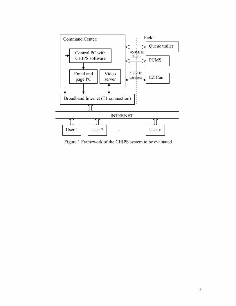
2. Framework and Operation of CHIPS 2.1 System Framework As shown in Figure 1, the CHIPS system is composed of devices in the field and hardware and software in the command center. The facilities in the field include quick queue trailers, EZ cam Mobile video trailers, and Portable Changeable Message Signs (PCMS). The quick queue trailer, which is employed as the speed sensor, can detect traffic changes in traffic flow. The main component of the quick queue trailer is the Remote Traffic Microwave Sensor (RTMS), made by Electronic Integrated Systems (EIS) Inc. PCMS displays real-time traffic information to travelers. The EZ cam is a trailer mounted Closed Circuit TV (CCTV) camera, used to monitor the traffic condition in the field. Each of these three devices communicates with the command center. The command center has the following hardware and software: communication systems (including a 450 MHz radio and 5.9 GHz wireless video antennas and receiver), AXIS 2400 video server, Email and page PC, and the control computer running the core CHIPS software. The command center communicates with quick queue trailers and PCMSs through a 450 MHz radio network, and the EZ Cams through a 5.9 GHz wireless video transmission system. The AXIS 2400 video server at the command center publishes surveillance video data received from the EZ Cams to the Internet. Users can remotely access the CHIPS system (i.e. the control computer) using software called PCAnywhere. The surveillance videos can be accessed using web browsers. Users can also receive messages from CHIPS through email (or page) if trouble conditions are observed. 2.2 Study Site and its Traffic Condition As shown in Figure 2, the work zone site is located in the City of Santa Clarita, north of Los Angeles, on freeway I-5, between Magic Mountain Parkway and Rye Canyon Road, a length of 1.3 miles. The construction started from July 30th, 2002 and left three lanes in each direction open to motorists after the closure of one southbound lane and one northbound lane on the median side. In case of traffic congestion, the Old Road is the suggested alternate route and has one lane in each direction in most places, with several signals and stop signs. Based on loop detector data and a set of on-site traffic condition observations conducted by Caltrans Traffic Management Team (TMT), it was found that southbound I-5 usually has severe traffic congestion in some Sundays and during holidays. 2.3 System Configuration

5

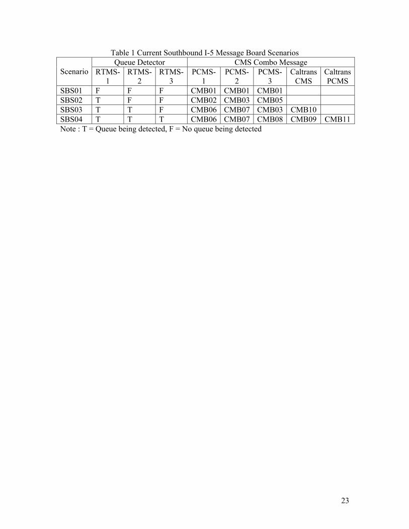
Caltrans and the system vendor designed the configuration of the system based on characteristics of the target work zone area. There are a total of five RTMSs, five PCMSs, and three CCTV cameras. In the southbound direction, there are three RTMSs and three PCMSs. Figure 2 shows a GIS-based CHIPS system map for the southbound approach. The distances from RTMS-1, RTMS-2 and RTMS-3 to the starting point of the construction are 0.15 miles, 1.19 miles and 2.40 miles, respectively. As a result, the maximum queue that the current system can detect is 2.4 miles. If traffic queues are longer than 2.4 miles (beyond the RTMS-3), Caltrans uses its own CMSs, i.e. “Caltrans PCMS” and “Caltrans CMS”, to provide information to travelers. “Caltrans CMS” is a fixed CMS facility located between Parker Rd and Hasley Canyon Rd. According to Caltrans, Caltrans did not invest additional money for more RTMSs and PCMSs in the CHIPS system because serious traffic congestion does not occur frequently in the site. Caltrans PCMSs and Caltrans CMS that are operated and controlled by field traffic engineers based on real-time traffic condition can be used as parts of CHIPS when there is serious congestion in the field. 2.4 System Setup CHIPS is an all-encompassing Traffic Management Package, which requires minimal programming to adjust to specific needs. Users need to self-define traffic management scenarios, which include traffic conditions and their corresponding traffic management schemes. When CHIPS detects a state change in any an RTMS, it will search for the traffic management scenarios that have been entered into the system. If a matching scenario is found, its corresponding messages will be shown on the PCMSs. After CHIPS sends out these new messages to PCMSs, it goes back to the polling routine. In other words, users need to determine what messages should be shown on PCMSs under a certain traffic congestion scenario. As shown in Table 1 and 2, Caltrans setup four scenarios for the southbound lanes. Scenario SBS01 corresponds to the situation that there is no traffic congestion and thus no message is shown on PCMSs. Scenario SBS02 corresponds to the scenario that only RTMS-1 has stopped or queued traffic and PCMS-1, PCMS-2, and PCMS-3 show messages CMB02, CMB03, and CMB05, respectively. Scenario SBS03 corresponds to the scenario that there is traffic congestion at RTMS-1 and RTMS-2 and thus the three PCMSs show messages CMB06, CMB07, and CMB03, respectively. Under this scenario, Caltrans CMS is also activated by Caltrans to show the following traffic information, “TRAFFIC JAMMED ROUTE 126 TO MAGIC MTN”. When all three RTMS locations are detected to have queued traffic, the three PCMSs show messages CMB06, CMB07, and CMB08, respectively. At the same time, Caltrans displayed traffic diversion information on its Caltrans CMS and Caltrans PCMS. 2.5 System operation Similar to other systems having been evaluated, the CHIPS system was found to have some technological problems, especially at the beginning of its operation. Examples of these problems include inappropriate initial setting of the system, inaccurate calibration of traffic sensors, communication, power and video system failure, and inability of the

6

control algorithm to correctly respond to a certain traffic condition. After a period of fine-tuning, the system started operating as desired with only occasional problems arising.

3. Diversion Effects As shown in Figure 2, there is only one alternative route, the Old Road, in the work zone area. If there is congestion on the southbound approach of the work zone, the use of CHIPS may have diversion effects. Vehicles on the southbound I-5 may take the Old Road via the Hasley Canyon Rd off-ramp or Lake Hughes Rd off-ramp. Vehicles on the eastbound SR-126 may take the Old Road via the Castaic Junction/Henry Mayo off-ramp. These diverted vehicles heading for I-5 southbound may take two on-ramps at Magic Mountain Blvd and Valencia Blvd to travel to I-5 southbound. The traffic pattern on the southbound I-5 is different for “weekdays” and “weekend & holidays”. In this paper, we will show only weekend & holiday analysis that definitely have diversion effects due to traffic congestion. For the analysis, the diversion rates and volumes at the Lake Hughes Rd off-ramp, Hasley Canyon Rd off-ramp, and Castaic Junction/Henry Mayo off-ramp will be estimated. 3.1 Data collection On-ramp and off-ramp traffic volume data were collected for the before scenario and after scenario. The before data were collected from May 13th to May 18th. We collected the after data during two time periods, Independence Day Holiday weekend (from June 30th to July 7th, 2003) and Labor Day Holiday weekend (from August 30th to September 2nd, 2003). After the traffic pattern analysis, we decided to use May 18th for the before scenario and Independence Day (July 6th) and Labor Day (Sep 1st) which show different traffic patterns for after scenarios. 3.2 Calculation of diversion Because the traffic demand and other traffic condition for the before and after scenario is hard to be the same in the real-world evaluation, a proportion-based method to estimate the diversion rate and diverted traffic volume is proposed in this paper. The proportion of the off-ramp traffic volume Voff with respect to the mainline traffic volume V can be calculated as follows:

VV

p off= (1)

If there is no diversion, we assume that the same proportion of the mainline traffic volume should exit at a certain off-ramp under both before and after scenarios. If there is diversion under the after scenario and there is no diversion under the before scenario, the diversion rate can be defined as the difference of the proportions of the after scenario (Pa) and the before scenario (Pb):

7

b

boff

a

aoff

ba VV

VV

pp −=−=α (2)

Va and Vb are the mainline traffic volume of the after and before scenarios which are calculated based on PeMS database available for each scenarios (6). The corresponding diversion traffic volume Vd can now be calculated:

ad VV ⋅= α (3)

If there is diversion under both scenarios, α and Vd correspond to the increase of the diversion rate and the increase of diversion volume. 3.3 Diversion estimation and analysis Using the methods described above, we estimated the diversion rates and diversion volumes at three off-ramp locations: Lake Hughes Rd off-ramp, Hasley Canyon Rd off-ramp, and SR-126 off-ramp to Castaic Junction / Henry Mayo, and the diversion volume at Valencia Blvd on-ramp. Figure 3 shows Hasely Canyon Off-ramp traffic proportions under the before and after scenarios, where you can see traffic diversion clearly. Table 3 shows the estimated time-dependent diversion rates and traffic volumes on Jul 6th, 2003 and Sep 1st, 2003. Figure 4 shows the diversion volumes at three off-ramps and the sum of diversion volumes with respect to the time of day. Figure 4 (a) and (b) show different diversion patterns at the Halsey Canyon Rd and Lake Hughes Rd off-ramps. Compared to the Lake Hughes Rd off-ramp, the Hasley Canyon Rd off-ramp is closer to the work zone and thus it has a longer period of traffic congestion. Based on Caltrans’ traffic report on July 6th, the maximum delay during the period of congestion was 47 minutes and occurred between 15:30 to 17:30. Figure 4(a) shows that the most serious diversions happened exactly during this time period. Based on Caltrans’ traffic report on September 1st, the maximum delay during the period of congestion was 33 minutes occurring between 17:30 and 20:00. Figure 4(b) shows that the greatest proportion of diversions happened at the hours of 17:00, 18:00, and 20:00. The traffic congestion of September 1st was not as severe as that of July 6th but the duration of congestion is longer. The total diversion volume of September 1st was lower than that of July 6th. 3.4 Travel time analysis The travel time data from Lake Hughes Rd to Valencia Blvd (collected by GPS-based probe vehicles on July 6th, 2003) are shown in Figure 5, in which the blue line and the purple line represent the travel time of the mainline freeway and the alternative route, respectively. The chart shows that when congestion occurred on the mainline, the travel

8

time along the alternative route was always less than that of the mainline. Most of the time, the alternative route would save about 3-4 minutes. The maximum time saving was about ten minutes, and occurred between the times of 14:15 and 15:04. The field observations showed that the queue on the freeway was between Hasley Canyon Rd and Lake Hughes Rd during this time period. The congestion data suggest that the alternative routes from Lake Hughes Rd to Valencia Blvd and from Lake Hughes Rd can save 3-4 and 2-3 minutes, respectively.

4. Safety Effects To evaluate the safety effect of the CHIPS system, the direct MOE is the number of collision accidents. The comparison of the collision data before and after the use of the system can be used to discover its contribution to the safety. Although the direct method is more simple and reasonable, it is hard to conduct because of a lot of uncontrollable factors. We conducted an accident analysis based on 10-month accident data collected from the study area. We did not include this part in this paper with the following reasons:

(1) the accident data source we used was PeMS database, which obtains accident data from CHP’s website and includes a lot of repeated accident data;

(2) During the study period, Caltrans performed a lane re-stripping, which caused the change of the work zone lane drop from the left side to the right side;

(3) there were not many accidents occurred in the 10-month period (from May 2003 to Dec 2003) and thus it hard to conclude any statistical decision.

Consequently, the focus of this study is to use indirect MOE to evaluate the safety effects of the system. A study showed that fatal accidents increase with higher speed limits (7). A couple of studies show that a major factor leading to an accident is the variation of speed. It was found that reducing the speed variation increases safety and reduces the likelihood of an accident (8, 9). Thus, vehicle speed and the variance in speed between vehicles may also be effective MOEs in the study of safety. Other research on traffic flow characteristics at freeway work zones found that the presence of a police patrol car on the shoulder of a busy freeway can stabilize the fluctuation of traffic flow by reducing both headway and the variability of headways (10). As a result, headway and its variance may also be effective MOEs in the study of safety. In this paper, the following traffic flow parameters were used as the indirect MOEs of safety effects:

(1) Traffic throughput (2) Traffic throughput (or volume) variance based on 1-minute throughput data (3) Sample speed mean (4) Variance of speed samples

These parameters above can be used to represent headway, variability of headways, speed and speed variance, respectively. 4.1 Data collection

9

Traffic count and speed data were collected using Jamar DB-100 counters and Bushnell Speed Guns at two measurement locations where RTMS-1 and RTMS-2 are located. The traffic count and speed data were collected at the same time, for a length of 30 minutes for both before and after scenarios. When we collected data at these two locations, the freeway traffic had been queued back to the far upstream of RTMS-2 location. As a result, we collected traffic data under queued traffic condition. The traffic count and speed data for the after scenario were collected between 16:53 and 19:31 on September 1st, 2003, during the Labor Day holiday. The traffic data of the before scenario were collected between 17:30 and 20:40 on August 17th, 2003, which was a Sunday during the summer. The CHIPS system stopped working at 15:53 because of a software conflict problem and all PCMSs were blank afterwards. This was the condition without CHIPS, which is regarded as the before scenario. The collected traffic count data were used for the analysis of traffic throughput and traffic volume variance. The collected speed samples were used for speed mean and speed variance analysis. 4.2 Traffic throughput Table 4 shows the lane-based traffic throughputs at the two measurement locations. Lane 1 represents the innermost lane in the table. Based on t-tests, significant differences (with 95% confidence interval) between before and after throughputs were observed at lane 1 of RTMS-1. Based on lane-based throughput data, the before-after lane distributions at two locations were obtained, as shown in Figure 6. The location 1 (RTMS 1) is related to an off-ramp and thus its traffic throughput is greatly affected by the off-ramp traffic. RTMS-1 is only 0.15 miles away from the work zone. Vehicles in lane 1 were required to merge to lane 2 because of the lane drop. CHIPS did not provide any lane closure information via PCMSs. Under both before and after scenarios, motorists obtained lane drop information from static signs, located prior to the RTMS-1 location. Compared to the before scenario (386 vehicles, corresponding to 17.8%), more throughput was found on lane 1 under the after scenario (466 vehicles, corresponding to 20.4%). Almost the same number of vehicles took lane 2 for both before and after scenarios. This indicated that higher traffic throughput was obtained on the mainline at RTMS-1 under the after scenario. The reason might be that a more stable traffic flow resulted because of CHIPS. As shown in Figure 3 and Table 5, the traffic flow was evenly distributed on each lane for both before and after scenarios at RTMS-2. This is because RTMS-2 is located at a place with less traffic weaving. 4.3 Variance of traffic volume Since both before and after scenarios were under congested traffic conditions, the variance of traffic volume can thus be used as a measure of the stability of queued traffic

10

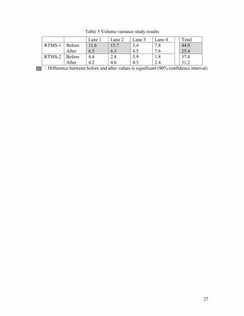
flow. Table 5 shows the variances of lane-based traffic volumes and grouped traffic volumes based on 1-minute throughput data. An F-test was conducted to see if the differences between variances of the before and after scenarios were significant (with 90% confidence interval). For the grouped traffic volume data, the difference of variance was significant at RTMS-1, which means that the variance of the after scenario was statistically smaller than that of the before scenario. For lane-based variance traffic volume data, the significant differences of variances were found for lane 1 and lane 2 at RTMS-1. These flow variance results suggest that traffic flow at RTMS-1 under the after scenario was more stable. The possible reason may have been that the messages on the portable signs made motorists drive more carefully and made them more aware of the static signs showing the lane drop information. 4.4 Speed mean and variance Literature reviews show that the mean driving speed is an appropriate measure of safety. The variance of speed is also an appropriate measure of the stability of traffic flow. A lower value of speed variance represents a more stable traffic condition. Table 6 summarizes the statistics of the speed sample data collected during the same time periods as those of traffic volume data, and Figure 7 shows the distribution of speed data at the two measurement locations graphically. To statistically compare speed variances of two populations for the before case and after case, an F test was conducted. F test results showed that the speed variances of the after scenario were significantly smaller than those of the before scenario at two measurement locations. This result implies that the traffic condition under the after scenario was more stable than the before scenario. Based on Z-test results, the average speeds at RTMS-1 and RTMS-2 were statistically the same for both before and after scenarios. This indicated that there were no driving speed difference between the before and after scenarios at RTMS-1 and RTMS-2, although a smoother traffic condition was obtained at these two locations based on the analysis on the speed variance data.

5 Driver survey A postcard-based survey was designed to obtain travelers’ comments on the work zone information system. The off-ramps at Lake Hughes Rd and Hasley Canyon Rd were selected as the driver survey locations. The travelers were asked to fill out the questions on the postcard and mail it back. Though this survey method only samples those travelers exiting the freeway via the two off-ramps, they are appropriate to be selected for commenting the system because the alternative route they are traveling on is very close to the freeway mainline. Travelers on the alternative route can see the mainline traffic condition and thus evaluate if they benefit from the diversion.

11

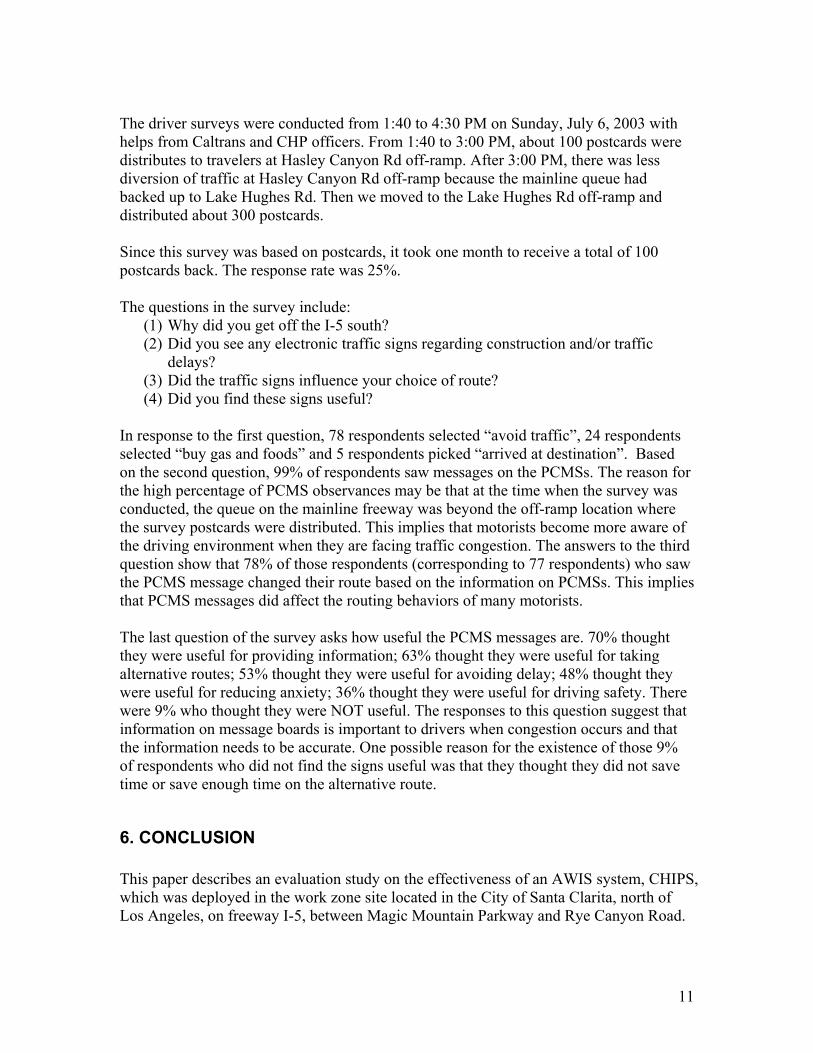
The driver surveys were conducted from 1:40 to 4:30 PM on Sunday, July 6, 2003 with helps from Caltrans and CHP officers. From 1:40 to 3:00 PM, about 100 postcards were distributes to travelers at Hasley Canyon Rd off-ramp. After 3:00 PM, there was less diversion of traffic at Hasley Canyon Rd off-ramp because the mainline queue had backed up to Lake Hughes Rd. Then we moved to the Lake Hughes Rd off-ramp and distributed about 300 postcards. Since this survey was based on postcards, it took one month to receive a total of 100 postcards back. The response rate was 25%. The questions in the survey include:

(1) Why did you get off the I-5 south? (2) Did you see any electronic traffic signs regarding construction and/or traffic

delays? (3) Did the traffic signs influence your choice of route? (4) Did you find these signs useful?

In response to the first question, 78 respondents selected “avoid traffic”, 24 respondents selected “buy gas and foods” and 5 respondents picked “arrived at destination”. Based on the second question, 99% of respondents saw messages on the PCMSs. The reason for the high percentage of PCMS observances may be that at the time when the survey was conducted, the queue on the mainline freeway was beyond the off-ramp location where the survey postcards were distributed. This implies that motorists become more aware of the driving environment when they are facing traffic congestion. The answers to the third question show that 78% of those respondents (corresponding to 77 respondents) who saw the PCMS message changed their route based on the information on PCMSs. This implies that PCMS messages did affect the routing behaviors of many motorists. The last question of the survey asks how useful the PCMS messages are. 70% thought they were useful for providing information; 63% thought they were useful for taking alternative routes; 53% thought they were useful for avoiding delay; 48% thought they were useful for reducing anxiety; 36% thought they were useful for driving safety. There were 9% who thought they were NOT useful. The responses to this question suggest that information on message boards is important to drivers when congestion occurs and that the information needs to be accurate. One possible reason for the existence of those 9% of respondents who did not find the signs useful was that they thought they did not save time or save enough time on the alternative route.

6. CONCLUSION This paper describes an evaluation study on the effectiveness of an AWIS system, CHIPS, which was deployed in the work zone site located in the City of Santa Clarita, north of Los Angeles, on freeway I-5, between Magic Mountain Parkway and Rye Canyon Road.

12

Three aspects of effectiveness studies were conducted, including traffic diversion, safety effects, and responses from travelers. The results of these studies showed that:

(1) Obvious diversion was observed on two evaluation dates because the travel time along the diversion route was shorter than freeway mainline during traffic congestion.

(2) Based on the study of the effects of traffic flow, the driving environment after the use of CHIPS seemed safer.

(3) Positive responses about the system were obtained based on driver surveys. Most survey respondents thought the system was useful for dispensing information, providing alternate routes, and avoiding delay.

Acknowledgements The evaluation team would like to thank many people from Caltrans who provide various devices, data, reports and information to us. Denis Katayama of District 7 deserves particular mention for his helps throughout the entire evaluation phase. We also would like to thank Professor Michael McNally of UC Irvine, who provided the GPS equipment for the study, Jun-Seok Oh of Western Michigan University, and Robert Tam and Chao Chen of UC Berkeley, who provided some good suggestions to this project.

REFERENCES

1. Scientex Corporation (1997) Final Evaluation Report For the Condition-Responsive Work Zone Traffic Control System (WZTCS). Prepared for the Maryland State Highway Administration and Federal Highway Administration, 1997.

2. Fontaine, M. D. (2003) Guidelines For The Application Of Portable Work Zone Intelligent Transportation Systems, In Transportation Research Record: Journal of the Transportation Research Board, No. 1824, TRB, National Research Council, Washington, D.C., 2003, pp. 15-22.

3. Agent, K.R. (1999) Evaluation of the ADAPTIR System for Work Zone Traffic Control, Report KTC-99-61, Kentucky Transportation Center, Lexington, Kentucky, November 1999.

4. McCoy, P.T. and Pesti, G. (2002) Effect of Condition-Responsive, Reduced-Speed-Ahead Messages on Speeds in Advance of Work Zones on Rural Interstate Highways. In Transportation Research Record: Journal of the Transportation Research Board, No. 1794, TRB, National Research Council, Washington, D.C., 2002, pp. 11-18.

5. Zwahlen, H.T. and Russ A. (2004) Evaluation of a Real-Time Travel Time Prediction System in a Freeway Construction Work Zone, In 81st Annual Meeting Preprint CD-ROM, Transportation Research Board, National Research Council, Washington, D.C., 2004.

6. Freeway Performance Measurement System (PeMS) Homepage: http://pems.eecs.berkerley.edu/, Nov. 11, 2004.

7. Raju, S., R. Souleyrette, and T.H. Maze. Impact of 65-mph speed limit on Iowa’s rural interstate highways. In Transportation Research Record 1640, TRB, National Research Council, Washington, D.C., 1992, pp. 47-56

8. Oh, C., Oh, S., Ritchie, S. and Chang, M. (2001) Real-time Estimation of Freeway Accident Likelihood, presented at TRB 2001

13

9. Thomas F. Golob and Wilfred W. Recker (2003), Relationships Among Urban Freeway Accidents, Traffic Flow, Weather, and Lighting Conditions, ASCE Journal of Transportation Engineering 129, pp. 342-353.

10. Polus, A. and Shwartzman, Y. (1999) Flow characteristics at freeway work zone and increased deterrent zones. Transportation Research Record 1657, pp. 18-23

14

List of Figures Figure 1 Framework of the CHIPS system to be evaluated Figure 2 Work zone site and CHIPS system setup Figure 3 Hasley Canyon Off-ramp traffic proportions under the before and after scenarios Figure 4 Estimation of the diversion traffic volumes Figure 5 Comparison of travel times along the mainline freeway and the Old Road Figure 6 Comparison of lane distributions at two measurement locations Figure 7 Speed distributions at two measurement locations

15

Field:

5.9GHz wireless

450MHz Radio

INTERNET

Command Center:

Control PC with CHIPS software

Video server

Email and page PC

Queue trailer

PCMS

EZ Cam

Broadband Internet (T1 connection)

User 1 … User 2 User n

Figure 1 Framework of the CHIPS system to be evaluated

16

Figure 2 Work zone site and CHIPS system setup

17

Hasley Canyon (Wkends)

0.00

0.04

0.08

0.12

0.16

0:00 4:00 8:00 12:00 16:00 20:00

Time of Day

Pro

porti

onBeforeAfter 1

Hasley Canyon (Wkends)

0.00

0.03

0.06

0.09

0.12

0.15

0:00 4:00 8:00 12:00 16:00 20:00

Time of Day

Pro

porti

on

BeforeAfter 2

(a) Weekend 1 (July 6th) (b) Weekend 2 (Sep 1st)

Figure 3 Hasley Canyon Off-ramp traffic proportions under the before and after scenarios

18

0

200

400

600

800

1000

11:00-12:00

12:00-13:00

13:00-14:00

14:00-15:00

15:00-16:00

16:00-17:00

17:00-18:00

18:00-19:00

19:00-20:00

Traf

fic v

olum

e

SR-126 Hasley Canyon Lake Hughes TOTAL

(a) Weekend 1: July 6th, 2003 (congestion period: 11:00 – 20:00)

0

200

400

600

800

11:00-12:00

13:00-14:00

15:00-16:00

17:00-18:00

19:00-20:00

21:00-22:00

Traf

fic v

olum

e

SR-126 Hasley Canyon Lake Hughes TOTAL

(b) Weekend 2: Sep 1st, 2003 (congestion period: 11:00 – 23:00)

Figure 4 Estimation of the diversion traffic volumes

19

0

4

8

12

16

20

24

28

10:00 12:00 14:00 16:00 18:00

Trip start time

Trav

el ti

me

(min

)

Freeway (Lake to Valencia) Alternative (Lake to Valencia)Freeway (Hasley to Valencia) Alternative (Hasley to Valencia)

Figure 5 Comparison of travel times along the mainline freeway and the Old Road

20

17.8% 22.5% 31.5% 28.2%

20.4% 21.1% 29.8% 28.7%

25.0% 24.6% 25.1% 25.2%

24.8% 24.7% 25.2% 25.3%

0% 25% 50% 75% 100%

RTMS1-before

RTMS1-after

RTMS2-before

RTMS2-after

Lane 1 Lane 2 Lane 3 Lane 4

Figure 6 Comparison of lane distributions at two measurement locations

21

0%

5%

10%

15%

20%

25%

0 10 20 30 40 50 60

Speed (mph)

% o

f tot

al

before (mean=29.9, std=8.9) after (mean=30.6, std=7.1)

0%

15%

30%

45%

60%

0 10 20 30 40 50 60

Speed (mph)

% o

f tot

al

before (mean=21.2, std=5.7) after (mean=21.0, std=3.7) (a) RTMS-1 (b) RTMS-2

Figure 7 Speed distributions at two measurement locations

22

List of Tables Table 1 Current Southbound I-5 Message Board Scenarios Table 2 List of Messages Table 3 Estimated diversion rates and diversion volumes Table 4 Traffic count data collected at two locations Table 5 Volume variance study results Table 6 Speed mean and variance

23

Table 1 Current Southbound I-5 Message Board Scenarios Queue Detector CMS Combo Message

Scenario RTMS-1

RTMS-2

RTMS-3

PCMS-1

PCMS-2

PCMS-3

Caltrans CMS

Caltrans PCMS

SBS01 F F F CMB01 CMB01 CMB01 SBS02 T F F CMB02 CMB03 CMB05 SBS03 T T F CMB06 CMB07 CMB03 CMB10 SBS04 T T T CMB06 CMB07 CMB08 CMB09 CMB11Note : T = Queue being detected, F = No queue being detected

24

Table 2 List of Messages Message Number Page 1(1st Flash) Page 2(2nd Flash) CMB01 BLANK BLANK CMB02 TRAFFIC/JAMMED SOUTH 5/AT RYE/CANYON CMB03 SLOW/TRAFFIC/AHEAD PREPARE/TO/STOP CMB04 TRAFFIC/JAMMED/NXT 2 MI EXECT/5MIN/DELAY CMB05 TRAFFIC/JAMMED/AHEAD 126 FWY/TO

MAGIC/MOUNTAIN CMB06 SOUTH 5/TRAFFIC/JAMMED AUTOS/USE NEXT/EXIT CMB07 JAMMED/TO

MAGIC/MOUNTAIN EXPECT/10 MIN/DELAY

CMB08 JAMMED/TO MAGIC/MOUNTAIN

EXPECT/15 MIN/DELAY

CMB09 TRAFFIC JAMMED TO MAGIC MTN

AVOID DELAY USE NEXT EXIT

CMB10 TRAFFIC JAMMED ROUTE 126 TO MAGIC MTN

CMB11 SOUTH 5 ALTERNAT ROUTE AUTOS USE NEXT 2 EXITS

25

Table 3 Estimated diversion rates and diversion volumes

(a) Data of Jul 6th, 2003 SR-126 Hasley Canyon Rd Lake Hughes Rd

Time period Rate Volume Rate Volume Rate Volume TOTAL

11:00-12:00 15.9% 126 1.3% 44 0% 0 170 12:00-13:00 17.6% 144 10.9% 482 0% 0 627 13:00-14:00 18.4% 134 12.0% 565 0% 0 699 14:00-15:00 20.9% 136 9.9% 483 4.0% 232 851 15:00-16:00 20.7% 133 8.4% 386 6.5% 364 883 16:00-17:00 20.5% 143 8.7% 405 6.9% 386 933 17:00-18:00 20.6% 117 8.1% 370 7.2% 395 881 18:00-19:00 17.8% 112 13.8% 442 0% 0 555 19:00-20:00 16.6% 99 2.2% 53 0% 0 152 TOTAL 18.7% 1144 8.7% 3231 6.1% 1377 5751

(b) Data of Sep 1st, 2003 SR-126 Hasley Canyon Rd Lake Hughes Rd

Time Rate Volume Rate Volume Rate Volume TOTAL

11:00-12:00 1.6% 11 0% 0 0% 0 11 12:00-13:00 11.7% 78 2.5% 65 0% 0 143 13:00-14:00 12.3% 74 8.1% 222 0% 0 297 14:00-15:00 15.6% 100 8.1% 258 0% 0 359 15:00-16:00 17.9% 122 10.3% 412 0% 0 534 16:00-17:00 23.5% 169 8.0% 373 0% 0 542 17:00-18:00 21.4% 142 5.1% 227 4.1% 211 581 18:00-19:00 25.9% 155 6.1% 240 5.4% 248 643 19:00-20:00 37.5% 207 5.2% 193 2.4% 103 503 20:00-21:00 36.5% 161 2.4% 101 8.3% 421 683 21:00-22:00 31.0% 95 7.2% 206 6.4% 213 514 22:00-23:00 29.5% 49 0.5% 7 0% 0 56 TOTAL 20.2% 1364 5.7% 2305 5.3% 1196 4865

26

Table 4 Traffic count data collected at two locations

Location 1 Location 2 Lane Before After Before After

1 386 466 517 479 2 487 482 509 478 3 682 680 520 487 4 612 656 522 488 Total 2167 2284 2068 1932

: Difference between before and after values is significant (95% confidence interval)

27

Table 5 Volume variance study results

Lane 1 Lane 2 Lane 3 Lane 4 Total Before 11.6 15.7 3.4 7.8 44.9 RTMS-1 After 6.5 6.3 4.5 7.6 25.4 Before 4.4 2.8 3.9 1.8 37.4 RTMS-2 After 4.2 4.6 4.3 2.4

31.2 : Difference between before and after values is significant (90% confidence interval)

28

Table 6 Speed mean and variance

# of samples

Sample Mean

Standard deviation

Sample variance

Before 979 29.9 8.9 80.0 RTMS 1 After 970 30.6 7.1 50.2 Before 1186 21.2 5.7 32.4 RTMS 2 After 993 21.0 3.7 13.5

: Difference between before and after values is significant (95% confidence interval)