transport energy air pollution model (team): methodology guide

1

Transport Energy Air pollution Model (TEAM): Methodology Guide

Dr Christian Brand (Environmental Change Institute, University of Oxford)

Prof Jillian Anable, Dr Ian Philips, Dr Craig Morton (Institute for Transport Studies, University of Leeds)

May 10th 2019

Working Paper

UKERC/DM/2019/WP/01

2

Introduction to UKERC

The UK Energy Research Centre (UKERC) carries out world-class, interdisciplinary research into sustainable future energy systems.

It is a focal point of UK energy research and a gateway between the UK and the international energy research communities.

Our whole systems research informs UK policy development and research strategy.

UKERC is funded by the UK Research and Innovation Energy Programme.

For information please visit: www.ukerc.ac.uk

Follow us on Twitter @UKERCHQ

Acknowledgements

The development of the modelling framework and supporting research was undertaken as part of the Decision Making Theme the UK Energy Research Centre.

The modelling framework was first developed for the European Commission in a collaborative effort across five European research organisations; the authors gratefully acknowledge the input of Mrs E Beckman, Dr W R Müller and Dr R Krüger for the early development of the tool. TEAM (and UKTCM beforehand) represent major upgrades and improvements in the approaches and methods used and the empirical datasets that have become available over the years.

http://www.ukerc.ac.uk/

3

Contents

List of Figures .............................................................................................................................. 5

List of Tables ............................................................................................................................... 6

List of Equations .......................................................................................................................... 7

Glossary of Terms ....................................................................................................................... 9

Executive Summary ................................................................................................................... 10

1. Introduction .......................................................................................................................... 11

1.1 Purpose of this Guide ...................................................................................................... 11

1.2 Setting the scene: strategic modelling of the transport-energy-environment system ..... 12

2. TEAM Overview ..................................................................................................................... 12

2.1 Approach ......................................................................................................................... 12

2.2 Background scenarios ...................................................................................................... 14

2.3 Policies and policy packages ............................................................................................ 16

2.4 The graphical user interface ............................................................................................ 17

2.5 The core modelling system .............................................................................................. 18

3. Transport Demand Model ..................................................................................................... 22

3.1 Approach ......................................................................................................................... 22

3.2 Overview of the demand modelling specification ............................................................ 24

3.2.1 Domestic passenger transport .................................................................................... 25

3.2.2 Freight ........................................................................................................................... 26

3.3 The main TDM inputs ...................................................................................................... 27

3.4 Demand model calibration – UK case .............................................................................. 31

4. Vehicle Stock Model .............................................................................................................. 33

4.1 Overview ......................................................................................................................... 33

4.2 Vehicle ownership ........................................................................................................... 36

4.2.1 Passenger cars .............................................................................................................. 36

4.2.2 Motorcycles .................................................................................................................. 43

4.2.3 Non-private vehicles .................................................................................................... 44

4.2.4 Buses and coaches ....................................................................................................... 44

4.2.5 Vans and trucks ............................................................................................................ 46

4.2.6 Passenger aircraft ......................................................................................................... 48

4.2.7 Freight aircraft .............................................................................................................. 50

4

4.2.8 Passenger and freight trains ........................................................................................ 51

4.2.9 Freight shipping ............................................................................................................ 52

4.3 Vehicle scrappage............................................................................................................ 53

4.3.1 Approach ...................................................................................................................... 53

4.3.2 Model specification ...................................................................................................... 54

4.4 Calculation of the total new vehicle stock ....................................................................... 57

4.5 Disaggregation of the total number of new vehicles by size or type ................................ 58

4.5.1 Passenger cars .............................................................................................................. 58

4.5.2 Vans and trucks ............................................................................................................ 60

4.5.3 Other vehicle types ...................................................................................................... 60

4.6 Vehicle technology availability ......................................................................................... 61

4.7 Vehicle technology choice ............................................................................................... 62

4.7.1 Passenger cars .............................................................................................................. 62

4.7.2 Vans and trucks ............................................................................................................ 69

4.7.3 Other vehicle types: motorbikes, buses, trains, shipping vessels, aircraft ............... 74

4.7.4 Technology distribution of the new vehicle fleet ....................................................... 78

4.8 Main outputs and links to other models .......................................................................... 78

4.8.1 Vehicle fleet distributions ............................................................................................ 78

4.8.2 Vehicle traffic distributions.......................................................................................... 79

4.8.3 Feedback to TDM – changes in generalised costs by mode of transport ................. 80

5. Direct Energy and Emissions Model ...................................................................................... 81

5.1 Overview ......................................................................................................................... 81

5.2 Model specification, data sources and calibration ........................................................... 82

5.2.1 Functional linkages for road transport ........................................................................ 82

5.2.2 Speed-emissions curves ............................................................................................... 84

5.2.3 Speed profiles ............................................................................................................... 86

5.2.4 Integration .................................................................................................................... 87

5.3 Scenario and policy modelling in the DEEM ..................................................................... 90

5.4 Model calibration ............................................................................................................ 91

6. Life Cycle and Environmental Impacts Model ........................................................................ 92

6.1 Approach ......................................................................................................................... 92

6.2 What the user can and ‘should not’ change .................................................................... 93

6.3 Modelling methodology .................................................................................................. 94

6.3.1 Life Cycle Inventory Model .......................................................................................... 94

5

6.3.2 Environmental Impact Assessment Model ................................................................. 98

6.4 Model Specification ....................................................................................................... 103

6.4.1 Definitions................................................................................................................... 103

6.4.2 Modelling flow within the LCEIM .............................................................................. 105

6.4.3 Functional relationships ............................................................................................. 107

6.4.4 Modelling equations .................................................................................................. 109

6.4.5 Key data sources ........................................................................................................ 110

7. Summary and Outputs ........................................................................................................ 111

References .............................................................................................................................. 112

List of Figures

Figure 1: Components of the Transport Energy Air pollution Model ......................................... 13

Figure 2: Screenshot of the main menu of the TEAM user interface ......................................... 18

Figure 3: Outline structure of the TDM ....................................................................................... 25

Figure 4: Screenshot of the TDM form to view and edit average transport cost elasticities ... 31

Figure 5: Historic and projected GDP growth rates and number of households for the reference scenario ........................................................................................................................ 32

Figure 6: Flow of calculations in the Vehicle Stock Model .......................................................... 35

Figure 7: Flow chart of how total car ownership is derived in TEAM......................................... 38

Figure 8: Van and truck fleet shares, private and business ........................................................ 46

Figure 9: Projected changes in shares of total road freight demand by vehicle type ............... 48

Figure 10: Scrappage probability function for selection of vehicle types .................................. 57

Figure 11: (a) Car market shares by vehicle ownership (private or fleet/company) and vehicle segment/size; (b) Car market shares by vehicle ownership (private or fleet/company) and consumer segment in the UK market (2015 data) ...................................................................... 58

Figure 12: (a) Private van/truck market shares by vehicle segment/type; (b) Business van/truck market shares by vehicle segment in the UK (2015 data) ......................................... 60

Figure 13: Outline of the car choice model within the TEAM modeling framework ................ 63

Figure 14: Outline of the van and truck choice model within the TEAM modeling framework........................................................................................................................................................ 70

Figure 15: Comparison of four hypothetical preference and performance parameter curves, other vehicle types (motorcycles, buses, trains, ships, aircraft, etc.) ........................................ 77

Figure 16: Scaling factor for simulating fuel, size and age dependence of car vehicle-km ...... 80

Figure 17: Interfacing of the DEEM and TNM models within TEAM .......................................... 81

Figure 18: Schematic overview of the functional linkages for road traffic ................................ 83

Figure 19: Schematic overview of the functional linkages for energy consumption and exhaust emissions from road transport ..................................................................................................... 84

Figure 20: View and edit ‘base’ emissions factors in DEEM ....................................................... 85

Figure 21: Base speed-emissions curves for fuel use and NOX emissions for small petrol cars86

Figure 22: Reference road speed profiles for cars, buses and trucks ........................................ 87

6

Figure 23: Example speed profiles for cars on motorways/double carriageways ..................... 87

Figure 24: Cross referencing and scaling of energy use and emissions factor datasets in the TEAM .............................................................................................................................................. 88

Figure 25: Variable linkages for modelling energy consumption and emissions....................... 88

Figure 26: Fuel consumption for petrol cars at 50 kph average speed ...................................... 89

Figure 27: Screenshot of the DEEM user forms for speed/congestion modelling .................... 90

Figure 28: User set up for driver behaviour change ................................................................... 91

Figure 29: LCEIM user interface, definition of model alternatives and policies ........................ 93

Figure 30: Life Cycle Inventory Model Linkages .......................................................................... 94

Figure 31: CO2 content of electricity on supply basis (incl. losses), reference scenario for the UK ................................................................................................................................................... 98

Figure 32: Environmental Impact Assessment Model Linkages ................................................. 99

Figure 33: Detailed modelling flowchart of the LCEIM ............................................................. 106

List of Tables

Table 1: Description of TEAM background scenario variables ................................................... 15

Table 2: List of the main policy options that can be modelled in TEAM, and their effects ...... 16

Table 3a: Summary of TEAM vehicle technologies for motorised passenger transport ........... 18

Table 4: The TEAM transport demand segments ........................................................................ 22

Table 5: Example of passenger travel demand indicators, Scottish ‘Lifestyle’ scenarios ......... 28

Table 6: Example of mode shift by trip length, Scottish ‘lifestyle’ scenarios ............................. 29

Table 7: The main motorcycle model assumptions .................................................................... 43

Table 8: The main bus model assumptions ................................................................................. 45

Table 9: The main truck and van model data and assumptions (1) ............................................. 47

Table 10: The main passenger aircraft demand modelling assumptions (1) .............................. 49

Table 11: The main freight aircraft demand modelling assumptions (1) .................................... 50

Table 12: The main train demand model assumptions (data shown are for 2015) .................. 51

Table 13: The main shipping demand model assumptions (2015 data) .................................... 53

Table 14: Scrappage parameters by vehicle type........................................................................ 56

Table 15: Consumer segmentation across private and company/fleet markets ....................... 59

Table 16: Vehicle attributes taken into consideration in the car choice model for private and fleet buyers .................................................................................................................................... 64

Table 17: Running cost price coefficients .................................................................................... 66

Table 18: Default technology preference (ASCi) values for plug-in vehicles.............................. 68

Table 19: Baseline price coefficients for fleet managers (based on 2012 ICE cars) .................. 68

Table 20: Vehicle attributes taken into consideration in the van and truck choice model for private and fleet buyers ................................................................................................................ 71

Table 21: Baseline price coefficients α for business buyers (based on 2015 diesel vehicles) .. 73

Table 22: Sample entry in output table Interface_VSM_NumVeh ............................................. 78

Table 23: Transport fuel specifications and indirect CO2 emissions factors from fuel supply .. 97

Table 24: Embedded emissions factors for fuel supply – example of diesel (DERV) ................. 97

Table 25: Damage types covered by the Environmental Impact Assessment Model ............... 99

Table 26: Pollutants and their main environmental impacts ................................................... 101

7

Table 27: Impact indicators ........................................................................................................ 102

Table 28: Abbreviations of variables used within the Life Cycle Inventory Model .................. 104

Table 29: Abbreviations of variables used within the Environmental Impacts Assessment Model ........................................................................................................................................... 104

Table 30: LCEIM attribute names and subscript labels ............................................................. 107

List of Equations

Equation 1: The main TEAM demand function ........................................................................... 27

Equation 2: The basic formula for vehicle stock evolution ......................................................... 33

Equation 3: Calculation of total car ownership ........................................................................... 39

Equation 4: Maximum car ownership for households owning at least one car ........................ 40

Equation 5: Maximum car ownership for households owning at least two cars, in urban areas........................................................................................................................................................ 40

Equation 6: Maximum car ownership for households owning at least two cars, in non-urban areas .............................................................................................................................................. 40

Equation 7: Maximum car ownership for households owning at least two cars, aggregated over geographical areas ................................................................................................................ 41

Equation 8: Maximum car ownership for households owning at least three cars .................... 41

Equation 9: Car ownership for households owning at least one or two cars ............................ 42

Equation 10: Car ownership for households owning at least three cars ................................... 42

Equation 11: Motorcycle traffic by vehicle size category ........................................................... 43

Equation 12: Total motorcycle ownership ................................................................................... 44

Equation 13: Bus traffic by vehicle size category ........................................................................ 45

Equation 14: Total bus ownership................................................................................................ 45

Equation 15: total number of vans and trucks ............................................................................ 46

Equation 16: Van and truck traffic by vehicle size category ....................................................... 47

Equation 17: Aircraft traffic by size category .............................................................................. 49

Equation 18: Total aircraft numbers ............................................................................................ 49

Equation 19: Total rail rolling stock .............................................................................................. 51

Equation 20: Train traffic by vehicle size category ...................................................................... 52

Equation 21: Total shipping stock ................................................................................................ 52

Equation 22: Shipping traffic by vehicle size category ................................................................ 53

Equation 23: Modified Weibull distribution ................................................................................ 55

Equation 24: Scrappage probability function .............................................................................. 55

Equation 25: Number of new vehicles needed ........................................................................... 57

Equation 26: Car choice model, utility function for private buyers ........................................... 63

Equation 27: Car choice model, market share for private buyers .............................................. 63

Equation 28: Car choice model, utility function for fleet manager segment ............................ 68

Equation 29: Van and truck choice model, utility function for private buyers .......................... 70

Equation 30: Van and truck choice model, market share for private buyers ............................ 70

Equation 31: Van and truck choice model, utility function for business/fleet buyer segment 73

Equation 32: Technology choice probability function ................................................................ 74

Equation 33: Annual cost of ownership and operation .............................................................. 75

8

Equation 34: Annual fuel costs ..................................................................................................... 75

Equation 35: Distribution of new vehicles by technology .......................................................... 78

Equation 36: Vehicle-km distribution by technology, vehicle type, size, fuel type and age ..... 79

Equation 37: Car vehicle-km distribution by technology and age .............................................. 79

Equation 38: Dependence of energy use and emissions on average speed .............................. 85

Equation 39: Direct Emissions .................................................................................................... 109

Equation 40: Number of vehicles requiring maintenance ........................................................ 109

Equation 41: Pro rata distribution by technology of additional infrastructure ....................... 109

Equation 42: Total material demand ......................................................................................... 109

Equation 43: Total fuel and energy demand ............................................................................. 109

Equation 44: Life cycle emissions, material supply ................................................................... 109

Equation 45: Life cycle emissions, fuel and energy supply ....................................................... 109

Equation 46: Life cycle emissions ............................................................................................... 109

Equation 47: Total emissions ...................................................................................................... 109

Equation 48: Primary energy requirements .............................................................................. 110

Equation 49: Land use of infrastructure .................................................................................... 110

Equation 50: External costs of direct emissions ........................................................................ 110

Equation 51: External costs of indirect emissions ..................................................................... 110

Equation 52: External costs of vehicle accidents ...................................................................... 110

Equation 53: Total external costs ............................................................................................... 110

Equation 54: Impact indicators .................................................................................................. 110

9

Glossary of Terms

TEAM Transport Energy and Air pollution Model, including country versions TEAM-UK (for the UK) and STEAM (for Scotland)

TEAM-UK Transport Energy and Air pollution Model for the UK

STEAM Scottish Transport Energy and Air pollution Model, i.e. TEAM for Scotland

TEAM UK Transport Carbon Model

TDM Transport Demand Model

VSM Vehicle Stock Model

DEEM Direct Energy and Emissions Model

LCEIM Life Cycle and Environmental Impacts Model

GDP/capita Gross Domestic Product per population

TEE transport-energy-environment

CO2 carbon dioxide

CO2e carbon dioxide equivalent (based on specified global warming potential)

CO carbon monoxide

VOC volatile organic compound

NMVOC non-methane volatile organic compound

NOx nitrogen oxides

PMx particulate matter (x=>10, <10, <2.5 micrometers)

C6H6 benzene

LH2 liquefied hydrogen

GH2 gaseous hydrogen

GHG greenhouse gases

LPG liquefied petroleum gas

CNG compressed natural gas

LNG liquefied natural gas

B100 100% biodiesel

HDV heavy duty vehicle

POCP photochemical ozone creation potential

GWP global warming potential

10

Executive Summary

Ever wondered how transport decision-making varies across individual (consumers), organisational (fleet managers, local authorities) and policy (central government) levels? Or how these decisions impact on energy systems? If so then quantifiable decision support tools may provide key supporting evidence on answering current policy questions such as the impacts and energy/transport interdependencies of road transport electrification, air pollution mitigation and dwindling energy tax revenues.

There is broad agreement on the need for substantial use of low carbon and local air pollutant vectors in the medium to long term in the transport sector. It is well known that societal energy consumption and pollutant emissions from transport are not only influenced by technical efficiency, mode choice and the pollutant content of energy, but also by lifestyle choices and socio-cultural factors. However, only a few attempts have been made to integrate all of these insights into systems models of future transport energy demand or even scenario analysis. Across the world a range of macro-economic and energy system wide, top-down models are used to explore the potential for reductions in energy demand, carbon emissions and air pollution in the transport sector. These models can lack the bottom-up, sectoral detail needed to simulate the effects of integrated demand and supply-side policy strategies to reduce emissions (Creutzig, 2015). There are also concerns that the pace and extent implied by many modelling studies is problematic and that assessment of (a) the heterogeneity in the market, (b) other low carbon vectors (e.g. conventional hybrids, hydrogen fuel cell) and (c) life cycle energy and environmental impacts have been relatively neglected.

Bridging the gap between short-term forecasting and long-term scenario models, the Transport Energy and Air pollution Model (TEAM) represents a major update of the UK Transport Carbon Model (Brand et al., 2017; Brand et al., 2012).

TEAM is a strategic transport, energy, emissions and environmental impacts systems model, covering a range of transport-energy-environment issues from socio-economic and policy influences on energy demand reduction through to lifecycle carbon and local air pollutant emissions and external costs. TEAM is built around exogenous and quantified scenarios, covering passenger and freight transport across all modes of transport (road, rail, shipping, air). It provides annual projections up to 2100, is technology rich with endogenous modelling of 1246 vehicle technologies, and covers a wide range of output indicators, including travel demand, vehicle ownership and use, energy demand, life cycle emissions of 26 pollutants, environmental impacts, government tax revenues, and external costs.

TEAM can be used to develop transport policy scenarios that explore the full range of technological, fiscal, regulatory and behavioural change policy interventions to meet climate change, energy security and air pollution goals.

This Methodology Guide describes the model in detail, including the overall methodology, core methods, functional relationships, data flows and main data sources.

11

1. Introduction

1.1 Purpose of this Guide

This Methodology guide describes the Transport Energy Air pollution Model (TEAM) in detail. The TEAM is a highly disaggregated, bottom-up system modelling framework of transport energy use and life cycle pollutant emissions. It provides annual projections of transport supply and demand, for all passenger and freight modes of transport, and calculates the corresponding energy use, life cycle pollutant emissions and environmental impacts year-by-year up to 2100. It takes a holistic view of the transport system, built around a set of exogenous scenarios of socio-economic and political developments. The model is technology rich and, in its current version, provides projections of how different technologies evolve over time for hundreds of vehicle technology categories, including a wide range of alternative-fuelled vehicles such as more efficient gasoline cars, hybrid electric cars, plug-in hybrid panel vans, hydrogen fuel cell trucks, battery electric buses and advanced aircraft. The current version (v2.5) includes 1,246 such vehicle technology categories. TEAM is specifically designed to develop future scenarios to explore the full range and potential of not only technological, but fiscal, regulatory and behavioural change transport policy interventions. Its high level outputs include travel demand, vehicle ownership and use, energy demand, annual and cumulative life cycle emissions, environmental impacts and external costs.

The latest version of TEAM provides significant improvements in three areas:

1. It extends previous market and consumer segmentation work for the private car market to the fleet and company car market and integrates this into a whole-systems transport-energy-environment modelling framework previously developed and applied in policy modelling studies (Anable et al., 2011a; Anable et al., 2012; Brand et al., 2013; Brand et al., 2012). This specifically addresses the need to integrate behavioural realism into whole systems transport-energy-environment models and to upscale the insights from place-based research and behavioral sciences (Creutzig, 2015; Sims et al., 2014).

2. It improves the way passenger travel demand is simulated over the longer term. By pursuing a more flexible approach that explores uncertainty in a scenario setting that originates in the Shell scenarios in the 1970s, TEAM now simulates passenger transport demand by simulating demand for travel with endogenously applied assumptions on how key drivers of travel demand affect trip patterns by trip purpose, trip distance, modal split, modal shift and occupancy rates, and how these may evolve over time (domestic passenger transport only). For freight transport and international aviation, demands are calculated endogenously year by year up to 2100 employing a typical econometric demand model.

3. It adopts a revised base year (2012) and longer timeframe (up to 2100) in line with energy systems and climate models such as TIMES/MARKAL. This should make it easier to couple and ‘soft link’ sectoral and economy wide models.

12

1.2 Setting the scene: strategic modelling of the transport-energy-environment system

Essentially three different approaches have been pursued for strategic modelling of the transport-energy-environment (TEE) system (for an overview see e.g. Burgess et al., 2005). This involves:

1. top-down equilibrium or optimisation models such as PRIMES (Syri et al., 2001) and MoMo (Fulton et al., 2009);

2. bottom-up simulation models such as TRENDS (Georgakaki et al., 2005), TREMOVE (De Ceuster et al., 2004), Zachariadis (2005) and Schäfer and Jacoby (2006), and;

3. transport network models such as ASTRA (Martino and Schade, 2000), SCENES (IWW et al., 2000) and EXPEDITE (de Jong et al., 2004).

The majority of these models were designed to explore specific policy questions, focusing on economic and technology policy interventions and their effects on transport demand, with some modelling of (direct) energy use and emissions. They often lack the detail necessary to model national low carbon policies that go beyond techno-economic policy options, e.g. policy aimed at changing travel behaviour. Models based solely on econometric approaches are deemed to be inappropriate for looking into the medium to long term future, as societies, preferences and habits (and thus elasticities) change.

At the national level a number of models exist, see e.g. de Jong et al. (2004). In the UK, no truly integrated (and independently operated) TEE model existed until the late 2000s, with policy makers relying on running different sets of models such as the (road) National Transport Model (NTM; DfT, 2005), with separate models for rail, aviation and navigation. In addition, transport and climate mitigation policy is informed by energy and economy systems modes such as the MARKAL/TIMES suite of models (Loulou et al., 2004), seeking to explore intra-sector dynamics and trade-offs. Although the models cover the majority of GHG emissions sources and types, they do not project full life cycle emissions. Finally, and crucially for the research community, assumptions and methods of government run models are often not explicit, making independent scenario planning and policy analysis difficult. The lack of an integrated policy-relevant life cycle model of carbon and local air pollutant emissions from transport was the main motivation for the development of the TEAM.

2. TEAM Overview

2.1 Approach

The TEAM provides annual projections of transport supply and demand, for all passenger and freight modes of transport, and calculates the corresponding energy use, life cycle emissions and environmental impacts year-by-year up to a set target date (up to 2100, depending on the policy or research question). It takes a holistic view of the transport system, built around a set of exogenous scenarios of socio-economic and political developments. The model is technology rich and, in its current version, provides projections of how different technologies

13

evolve over time for more than 1200 vehicle technology categories, including a wide range of alternative-fuelled vehicles such as more efficient gasoline cars, hybrid electric cars, plug-in hybrid vans, battery electric buses and advanced aircraft. However, the TEAM is specifically designed to develop future scenarios to explore the full range and potential of not only technological, but fiscal, regulatory and behavioural change transport policy interventions. Figure 1 provides an overview of the system components which include:

1. a set of quantified scenarios which describe a range of possible external political and socioeconomic developments envisaged up to 2100;

2. a set of single policy options and multiple policy packages that include fiscal, technical, regulatory and demand management measures;

3. four linked models of the transport-energy-environment system, and;

4. a graphical user interface, to set up and run the model and view key modelling results.

Figure 1: Components of the Transport Energy Air pollution Model

Together with the policy and scenario components, the models are linked by:

common tables, containing definitions of variables that are used in more than one model;

TEAM modelling framework

scenario variables(e.g. GDP/cap, demographics,

income, pre-tax fuel prices)

policy variables(e.g. road taxes, pricing, speed

limits, driver behaviour)

transport demand (pkm, tkm)

vehicle stock (total, new, scrapped)

energy & emissions(direct: vehicle use, TTW)

energy & emissions(indirect: fuel WTT and vehicle manufac., maint. and disposal)

lifecycle energy & emissions(direct and indirect)

view & export results(Access, Excel)

partial equilibrium

environmental impacts and costs(e.g. GWP, health impacts of air pollution,

external costs of climate change and air pollution)

input

phase

modelli

ng p

hase

analy

sis

phase

14

interface data tables, containing all the variables and values which need to be transferred from one model to a subsequent model and to the results database;

the results database, containing all the simulation modelling results the user might be interested in, calculated for a user-defined set of alternatives1. The main outputs include travel demand, vehicle stock, energy and fuel demand, fuel tax revenues, annual and cumulative life cycle emissions, environmental impacts and external costs.

2.2 Background scenarios

The basic idea of using ‘background’ scenarios in TEAM is to introduce wider contextual factors and consideration of uncertainty into the analysis of transport policy and technology take-up. The set of background scenarios describes a range of possible external political and socio-economic developments envisaged to 2100 or earlier. In TEAM, up to four exogenous scenarios can be developed as four internally consistent possible futures. The futures are quantitatively specified by a set of exogenous variables which may affect the outcomes of the models, while being outside the control of the transport-energy-environment system. These variables include changes in national GDP, pre-tax energy prices, demographics, household disposable income and maximum car ownership levels. The purpose of the scenarios is to provide a series of contexts within which the UK transport system may develop over time so that alternative policies can be tested for robustness against the uncertainties in the political, socio-economic and technological spheres.

Each background scenario in TEAM can describe an internally consistent trajectory of exogenous development for the next 40 years or so. Together, the background scenarios are meant to span the credible range of uncertainties of interest to stakeholders. When talking about exogenous developments, we mean factors that are external relative to the transport system in the UK but nevertheless salient to its evolution, and specifically to the evolution of transport demand and the deployment of transport technologies. Factors internal to the British transport system are, in principle, to be dealt with in the modelling chain of the TEAM system.

Driving forces, which are high in impact and uncertainty, are at the core of the scenarios. These can be identified and characterised through extensive consultation with external experts, as performed in similar exercises around the world (see e.g. the visioning work by Hickman and Banister, 2006). The resulting scenarios should highlight different developments along the “dimensions” of governance and people’s values and perceptions, primarily in the UK. In order that the set of scenarios covers a sufficiently wide range of possibilities, each scenario is relatively extreme – albeit plausible. Descriptions of the most likely developments would be of little help in coping with uncertainty.

Of course, a set of four scenarios cannot cover all possible combinations of variations in external factors. Developments and occurrences that are weakly linked to the core features

1 Each alternative represents one combination of scenario and policy package. For example, different levels of gasoline and diesel taxation could be defined and calculated as a set of alternatives.

15

of any specific scenario may occur in any of the four scenarios. This could e.g. be shock events, a new oil crisis or different trajectories for demographic data.

In modelling terms, the set of scenarios provides input data to the TEAM modelling system according to a vector of scenario variables, shown in Table 1. For each variable, scenario and year, data are given in a scenario database. The TEAM system provides default data for all variables. The user can modify these variables that do not relate strongly to core features of the scenarios, within certain limits. (Such variation is actually recommended, to provide a sensitivity/uncertainty analysis.)

Table 1: Description of TEAM background scenario variables

Description Form of variable Can be modified by user?

Annual rate of GDP growth %, per year Yes

Number of households index Index relative to base year Yes

Fuel price index (pre-tax):

Crude oil

Natural gas

Biomass

Electricity

Index relative to base year Yes

Vehicle price index (pre-tax), for small, medium and large cars


Load factor index (by vehicle type, urban and non-urban)


Electricity generating mix % share, for each year, of crude oil, coal, hydro, natural gas, photovoltaics on buildings, nuclear, biomass, wind & wave, imports to total electricity generated

Yes

Extra-UK freight growth rate %, per year Yes

Changes in

average speed (motorway, rural roads)

frequency of cold starts

idling time

% change over the period base year-2100. Used as a look-up table to guide user modification of assumptions entered in the DEEM, rather than as a direct quantitative input.

Yes

Change in transport intensity of GDP

passenger

freight

Index relative to base year, influencing the elasticity of transport demand

No

Index of passenger transport split

private car

public transport

air


Yes

Index of freight transport split

road

rail


Yes

16

Description Form of variable Can be modified by user?

Split of demand between journey segments for car trips

urban

rural

motorway


2.3 Policies and policy packages

The policy options include fiscal measures such as vehicles and fuel taxes, regulatory measures such as fuel economy standards, information and education policies and investment and planning policies. Table 1 provides a list of the main policy options that can be modelled in TEAM, and their primary and secondary effects. Importantly, policy packages of two or more policies listed in the Table can be modelled at the same time in an integrated and internally consistent manner.

Table 2: List of the main policy options that can be modelled in TEAM, and their effects

Policy Primary (and secondary) effects Model

Fiscal

Company car tax fleet car technology choice, (demand) VSM/TDM

Vehicle circulation tax road vehicle technology choice, (demand) VSM/TDM

Vehicle purchase tax / feebates vehicle technology choice, (demand) VSM/TDM

Car scrappage incentive/rebate private car technology choice, car ownership, (demand)

VSM/TDM

Fuel taxation (by volume or carbon and local air pollutant content)

vehicle technology choice, (demand) VSM/TDM

Road user/congestion charging (graduated)

vehicle technology choice, (demand) VSM/TDM

Parking charges vehicle technology choice, (demand) VSM/TDM

Regulation

Fuel economy standards (voluntary, compulsory)

Technology innovation in new vehicle fleets, vintaging (demand)

VSM/TDM

Regulation for low rolling resistance tyres and tyre pressure monitoring

vehicle emissions factors DEEM

Speed limits and enforcement road vehicle speed profiles and emissions factors

DEEM

Fuel obligations (e.g. Renewable Transport Fuel Obligation)

carbon and local air pollutant content of blended fuel, vehicle emissions factors

DEEM

Low emission zones (carbon and local air pollutant)

‘redistribution’ of traffic to low emissions vehicles in access areas (e.g. urban)

VSM

17

Policy Primary (and secondary) effects Model

High occupancy vehicle lanes average load factors, (average speeds and emissions)

VSM, (DEEM)

Information, education, smart/soft measures

Travel plans (individualised, residential, workplace, schools)

travel activity, modal shift, average distance travelled by car

Scenario

Eco-driving / driver behaviour vehicle emissions factors DEEM

Labelling technology choice (via preference parameter)

VSM

Car sharing / pooling load factors, car demand VSM/TDM

Planning and investment

Parking space availability car ownership (second, third+ car) VSM/TDM

Rail electrification direct emissions, indirect emissions (electricity generation)

Changes in electricity generation indirect emissions from (plug-in, battery) electric vehicle use

LCEIM

Additional public transport infrastructure, e.g. high speed rail investment

indirect emissions from manufacture, (modal shift, induced demand)

LCEIM, (Scenario)

Note: TDM = transport demand model, VSM = vehicle stock model, DEEM = direct energy use and emissions model, LCEIM = life cycle and environmental impacts model.

2.4 The graphical user interface

The user accesses the model mainly via a newly developed graphical user interface (GUI) which serves as the main portal for setting up the exogenous scenarios, endogenous policies and policy packages, running of the modelling chain, visualisation of the results in tabular and graphical form, and semi-automated export to Excel or similar analysis software packages. TEAM has been developed in Microsoft Access (v2010) as a relational database system. The main menu form of the GUI is shown in Figure 2. For further information on how to use TEAM refer to the existing UKTCM user guide (Brand, 2010), which is available to download from the UKERC website (www.ukerc.ac.uk).

http://www.ukerc.ac.uk/

18

Figure 2: Screenshot of the main menu of the TEAM user interface

2.5 The core modelling system

The four linked simulation models represent the core of the modelling system and describe the transport system and calculate their impacts. They are:

1. the transport demand model (TDM);

2. the vehicle stock model (VSM);

3. the direct energy use and emissions model (DEEM) and;

4. the life cycle and environmental impacts model (LCEIM).

The TDM calculates the overall level of transport activity and modal shares for passenger and freight movements. The VSM tracks the changes in the vehicle stock brought about by the overall demand for vehicles, the scrapping of old vehicles and the purchasing of new vehicles – potentially using new or improved propulsion technologies. This is highly disaggregated and involves comparing hundreds of alternative vehicle technologies in any year, totalling over 1,240 technologies that are ‘vintaged’ in order to simulate innovation over time. Table 3a summarises this for passenger and Table 3b for freight transport technologies. The outputs of the VSM are the total vehicle kilometres and number of vehicles (split by technology) each year.

Table 3a: Summary of TEAM vehicle technologies for motorised passenger transport

Vehicle type Size Primary fuel Engines/ drivetrains No. of vintages/ innovations

Car Small Gasoline ICV, HEV, PHEV 29

(A/B segments) Diesel ICV 10

Electric Battery EV 12

H2, LPG, CNG FC, ICV 20

Medium Gasoline ICV, HEV, PHEV 30

(C/D segments) Diesel ICV, HEV, PHEV 30

19


Biodiesel (B100) ICV 3

Bioethanol (E85) ICV 9

LPG, CNG ICV 20

H2 FC 2

Large Gasoline ICV, HEV, PHEV 30

(C/D segments) Diesel ICV, HEV, PHEV 30




LPG, CNG ICV 20

H2 FC 2

Motorcycle (one size) Gasoline ICV 3


H2 FC 2

Bus Mini Gasoline ICV 3

Diesel ICV, HEV 22


LPG, CNG ICV 18



H2 FC 1

Urban Diesel ICV, HEV, PHEV 30


LPG, CNG ICV 18



H2 FC 6

Coach Diesel ICV, HEV 22


LPG, CNG ICV 18


H2 FC 6

Rail Light, metro, urban Diesel ICV 3

Grid electricity Electric 3

Regional Diesel ICV 3


Intercity Diesel ICV 3


High speed Grid electricity Electric 3

Air General aviation Jet A-1 Turboprop 1

Short haul, dom. Jet A-1, Bio jet Turbine 9

Medium haul, int. Jet A-1, Bio jet Turbine 9

Long haul, int. Jet A-1, Bio jet Turbine 9

Supersonic, int. Jet A-1, Bio jet Turbine 9

20

Table 3b: Summary of TEAM vehicle technologies for motorised freight transport

Vehicle type Size Fuels Engines/ drivetrains No. of vintages/ innovations

Trucks & Six van types: Gasoline ICV 73

Vans Panel & side Diesel ICV, HEV, PHEV 175

Car derived Electric Battery EV 60

Pickup & 4x4 Biodiesel (B100) ICV 54

Drop & Tipper Bioethanol (E85) ICV 54

Box, Luton, Insul. LPG, CNG ICV 114

Other H2 FC 36

Medium HGV Diesel ICV, HEV 14

(3.5t - 16t GVW, Electric Battery EV 3

+non-articulated) Biodiesel (B100) ICV 4

LPG, CNG ICV 19

H2 FC 7

Large HGV Diesel ICV, HEV 15

(>16t GVW, Biodiesel (B100) ICV 4

+articulated) LPG, CNG ICV 19

H2, biomethanol FC 7

Rail Regional Diesel ICV 3


Shipping Inland Diesel ICV 2

Coastal Diesel ICV 2

Maritime Diesel ICV 2

Air Short haul, dom. Jet A-1, Bio jet Turbine 9

Medium haul, int. Jet A-1, Bio jet Turbine 9

Long haul, int. Jet A-1, Bio jet Turbine 9

Supersonic, int. Jet A-1, Bio jet Turbine 8

Where: HGV=heavy goods vehicle; LCV=light commercial vehicle; GVW=gross vehicle weight; ICV=internal combustion engine vehicle; HEV=hybrid electric vehicle; PHEV=plug-in hybrid electric vehicle; H2=hydrogen (gaseous or liquid); B100=100% biodiesel; E85=85% bioethanol-15% gasoline blend; LPG=liquefied petroleum gas; CNG=compressed natural gas; dom.=domestic; int.=international; Jet A-1=aviation jet fuel (kerosene)

The DEEM takes data from the VSM to calculate direct2 emissions and energy consumption due to the different vehicle technologies that comprise the vehicle fleet. The model produces information on emissions of carbon dioxide (CO2), carbon monoxide (CO), nitrogen oxides (NOX), sulphur dioxide (SO2), total hydrocarbons (THC) and particulate matter (PM). (The DEEM can also be linked to a Traffic Noise Model (TNM) which estimates the areas

2 ‘Direct’ also refers to ‘tailpipe’, ‘source’ or ‘end use’.

21

affected by various levels of noise.) The LCEIM has two functions. First, it provides an energy and emissions life cycle inventory due to the manufacture, maintenance and disposal of vehicles, as well as infrastructure contributions (e.g. embedded emissions from building high speed rail tracks). The inventory also provides energy use and emissions over the fuel production cycles for the different fuels used by different vehicle technologies. Secondly, the LCEIM estimates the environmental impacts of the overall levels of emissions by providing a series of ‘impact indicators’, such as global warming potential, as well as monetary valuation of the damage associated with such emissions levels (external costs).

22

3. Transport Demand Model

3.1 Approach

The function of the transport demand model (TDM) is to project transport demand for the years up to 2100. As future demand for transport is highly uncertain, the aim of the TDM is merely to develop a set of plausible developments of transport demand as a function of scenario variables (such as changes in populations, incomes, fuel prices and demographics) and costs of current and future transport technologies.

Given the timescale involved, the TDM is not intended to provide an accurate prediction of the most likely future development of transport demand. The choice of the appropriate modelling approach has been determined by a trade-off between the required high level of detail and the availability of data.

In order to disaggregate the results for about 20 transport demand categories, a hybrid approach of combining detailed simulation of passenger travel patterns with econometric modelling of freight and international aviation demand. For each of the main modes of transport (Table 4), demand is either:

simulated with endogenously applied assumptions on how key drivers of travel demand affect trip patterns by trip purpose, trip distance, modal split, modal shift and occupancy rates, and how these may evolve over time (domestic passenger transport only), or;

calculated endogenously year by year up to 2100 employing a typical econometric demand model (freight transport and international aviation).

In the simulation, passenger demand is essentially decoupled from traditional econometric forecasting in that the user specifies key drivers of demand, including changes to trip frequencies by purpose (e.g. commuting, shopping), mean distances and occupancy rates by mode. This allows exploring more radical changes in travel patterns, lifestyles and systemic changes that are not easy to model using standard econometric techniques that essentially project historic choices (revealed through elasticities of demand) into the future.

In the simple econometric model, the evolution of demand for freight (and international aviation) depends on exogenous scenario parameters such as future estimates of GDP/capita, the number and structure of households and the population’s propensity to travel. It is also affected by the evolution of energy prices and average ownership and operating costs for each vehicle type, dependent on the technologies in the vehicle fleet and the levels of taxation, via a feedback loop from the vehicle and policy cost sub-modules.

This hybrid approach aims to provide a set of plausible developments of transport demand – it is not intended to provide an accurate prediction of the most likely future development of transport demand to 2100.

Table 4: The TEAM transport demand segments

Passenger demand segments Freight demand segments

Mode Journey segment Mode Journey segment

Walking Urban LCV (vans) Urban

23

Cycling Urban / non-urban Rural

Motorcycle Urban Motorway

Rural HGV (trucks) Urban

Motorway Rural

Car Urban Motorway

Rural Rail Dedicated rail freight

Motorway Navigation Inland / domestic

Bus Local bus (urban) Coastal / domestic

Coach (motorway) Maritime / intern.

Minibus (rural) Air freight Domestic short haul

Rail Light rail and underground International medium haul / Europe

Regional rail International long haul / intercontinental

Intercity rail International supersonic

High speed rail

Passenger air

Domestic short haul

International medium haul / Europe

International long haul / intercontinental

International supersonic

Where: HGV=heavy goods vehicle (trucks over 3.5t GVW); LCV=light commercial vehicle (vans 1-3.5t GVW)

The amount of demand calculated in the TDM influences the development of prices in the Vehicle Stock Model (VSM) in the same year. The development of prices in the VSM then influences the development of demand in the TDM in the following year. This allows us to calculate a near-equilibrium between supply and demand. The final outputs of the demand model are passenger transport demand (expressed in passenger-kilometres), freight transport demand (expressed in tonne-kilometres) and passenger occupancy rates (load factors for freight) for the demand segments summarised in Table 4.

The approach outlined above is deemed appropriate for the following reasons:

The development of passenger transport demand (in passenger-km) is dependent on changes in demographic, socio-economic and structural factors, including changes in transport costs/prices, land use, employment patterns, access to and use of ICT, and so on. GDP/capita is less of a factor for passenger demand than for freight.

The development of freight transport demand (in tonne-km) is strongly dependent on GDP/capita and population growth as well as structural changes (land use, logistics).

The freight elasticities used in the TDM can vary from year to year. This reflects a change in consumption preferences and avoids a simple translation of the developments of the past into the future.

24

The freight elasticities used are short-run elasticities and reflect the dependence of transport demand on GDP/capita and population growth in a given period – in a single year in TEAM. Studies have shown that there is a difference between short-run and long-run transport demand elasticities. In the short run, incomes/prices influence the spontaneous decision of making a trip and also the decision concerning which transport mode is used (e.g. in the short run, a van has already been purchased and ‘only’ the variable costs of a trip are decisive). In contrast, in the long-run, changes in incomes and prices can lead to a lasting change in consumer/business behaviour and can also influence the vehicle purchase decision. This difference between short-run and long-run effects has been taken into account in an indirect way in TEAM. On the one hand, the elasticities used in the TDM reflect the short-run effects of prices/costs on transport demand. On the other hand, the VSM handles long-run effects on transport demand like vehicle purchasing cost, which are transmitted to the TDM via the average transport costs.

The design of the TEAM does not allow for a feedback between transport prices and GDP, which would be desirable from a theoretical point of view, but can only be realised with a complex (combined economic and transport demand) modelling approach performed by an equilibrium modelling software like GAMS. However, from a practical point of view this is not necessary as long as the policy effects (of raising fuel duty, for example) are moderate. A good way to estimate the effect of the missing feedback would be to compare TEAM with an economy-wide systems model. The transport demand results, the changes in transport costs and the amount of transport taxes over the modelling years obtained from a TEAM modelling run could be used as input for an economic model. This would show the effect on the development of GDP and a possible correction to the GDP scenario to be used in a repeat of the modelling run. This type of modelling exercise was performed during the Energy2050 project at the end of UKERC Phase I.

3.2 Overview of the demand modelling specification

At the top level transport demand is split into passenger transport (the demand for transporting people) and freight transport (the demand for transporting goods). Figure 3 outlines the structure of the TDM. Based on scenario, context and policy variables such as demographic, socio-economic and fuel tax projections, step A calculates overall transport demand for passenger and freight. In step B changes in modal make up of total passenger and freight demands are derived on the basis of relative changes in average ownership and operating costs for each mode. The relative changes of supply costs for each mode of transport fed back from the VSM lead to an income effect influencing the level of demand and a substitution effect causing a change in the relative transport volume shares for each mode. Step C merges the outputs of steps A and B, checks for internal consistency and finally provides modal shares for each demand segment.

25

Figure 3: Outline structure of the TDM

3.2.1 Domestic passenger transport

In step A, the passenger transport demand model simulates passenger travel demand as a function of key travel indicators structured around data obtained from the UK National Travel Survey (DfT, 2016), including the average number of trips and average distance travelled per person per year. These were further disaggregated by seven main trip purposes:

1. commuting, 2. business, 3. long distance leisure, 4. local leisure, 5. school/education, 6. shopping, 7. other.

For each of those the demand model disaggregates trip frequencies by eight trip lengths:

1. under 1 mile, 2. 1-2 miles, 3. 2-5 miles, 4. 5-10 miles, 5. 10-25 miles, 6. 25-50 miles, 7. 50-100 miles, and

Policy and Context Variables(e.g. GDP, fuel tax, elasticities)

B: Calculating modal shift Output: shif ts in passenger km / tonne km by mode

A: Calculating total transport demand Output: aggregate passenger km / tonne km

Input from the VSM:average ownerhsip and operating costs/prices for

each vehicle type, RC

C: Calculating modal shares

Outputpassenger km / tonne km by mode

26

8. more than 100 miles.

Passenger transport is further disaggregated by twelve modes of passenger transport:

1. walk, 2. bicycle, 3. car/van driver, 4. car/van passenger, 5. motorcycle, 6. local bus, 7. coach, 8. rail and underground, 9. other private including shared taxi, 10. taxi, 11. domestic air, 12. other public.

International air travel is modelled separately as a function of income (GDP/capita), population and supply and policy costs (see next section).

TEAM-UK was calibrated to UK national statistics for the year 2012 (DfT, 2014d). We obtained Special Licence Access to the National Travel Survey dataset (DfT, 2016) and used SPSS v23 to derive average trip rates, distance travelled and mode splits for the UK. A similar exercise was undertaken to set up and calibrate the Scottish version, STEAM.

Default (i.e. reference) transport demand projections are usually simulated based on ‘no changes’ in trip patterns3 (i.e. trips and distance travelled per person p.a., and mode split) apart from lower commuting levels due to an ageing population, and average demand elasticities (of GDP/capita, population and generalized cost) for international air and freight transport (Dunkerley et al., 2014; Sims et al., 2014). In contrast, alternative demand projections can be modelled by changing the underlying drivers. For example, recent work on Scotland analyzed consequences for travel patterns of future changes to ‘lifestyles’ and social norms. This took as its starting point the figures for current individual travel patterns based on Scottish data in the UK National Travel Survey (DfT, 2016). The Scottish data was analyzed so as to derive figures for each journey purpose (commuting, travel in the course of work, shopping, education, local leisure, distance leisure and other) in terms of average number of trips, average distance (together producing average journey length). In addition, mode share and average occupancy were altered based on an evidence review (e.g., Cairns et al., 2004, 2008; Petrunoff et al., 2015; Scottish Government, 2013) relating to the impact of transport policies and current variation in travel patterns within and outside Scotland.

3.2.2 Freight

Total freight demands are derived using a simple transport demand function that relates demand (dependent variable) with explanatory variables such as scenario context variables, policy variables and other TEAM input variables. In essence, freight demand is simulated as a

3 This applies to the Reference case only. Average distance travelled vary by propulsion technology (e.g., diesel cars travel further per year than petrol or EV cars, based on national statistics).

27

function economic activity (GDP/capita) and population, with reference demand elasticities taken from a RAND Europe study (Dunkerley et al., 2014). Steps A and B can be summarised in an econometric function of exogenous parameters, together with their respective elasticities of demand. This takes on the form shown in Equation 1:

Equation 1: The main TEAM demand function

ERC

n

n

ENHH

n

n

EGDP

n

n

n

n

RC

RC

NHH

NHH

GDP

GDP

T

T

1111

**

where T = demand for travel (expressed in passenger-km and tonne-km)

GDP = Gross Domestic Product

NHH = total number of households

RC = relative vehicle ownership and operating costs

EX = elasticity with respect to X

n = modelling year (currently 2012, 2013, …, 2100)

As mentioned above, in the short run incomes/prices influence the spontaneous decision of making a trip and also the decision concerning which transport mode is used. In contrast, in the long-run, changes in income and in prices can lead to a lasting change in people’s behaviour and can also influence vehicle purchase decisions (for a good review see Goodwin et al., 2004). The difference between short-run and long-run effects has been taken into account in an indirect way in TEAM. The first two elasticities in Equation 1 reflect the short-run effects of changes in prices/costs/population on transport demand. The third elasticity reflects the long-run effects of relative changes of vehicle ownership and operating costs as fed back by the vehicle stock model.

To avoid a simple static approach the elasticities can take different values for each future year up to 2100. This dynamic approach allows modelling change in behaviour and preferences and avoids a simple projection of the past into the future. The estimation of the parameters for the calculation of future demand is based on statistical data for previous years and on transport demand forecasts taken from other studies. This allows the researcher and user to specify a ‘base case’ or ‘reference’ scenario against which alternative scenarios are compared.

3.3 The main TDM inputs

The TDM uses a number of parameters to determine transport demand, which can all be readily modified by the user. The parameters can be divided into five groups.

In the first group are income elasticities and population growth elasticities for each of the demand segments listed in Table 4. The income elasticities represent the dependence of transport demand growth on growth of income measured as GDP. The population growth

28

elasticities reflect the dependence of transport demand on the development of the population measured as the number of households.

The second group concerns the passenger transport demand module, which requires trip frequencies, average trip lengths and mode shifts by trip length. As an example, the Scottish ‘lifestyle’ scenario values are shown in Table 5 and

Table 6 below.

Table 5: Example of passenger travel demand indicators, Scottish ‘Lifestyle’ scenarios

2012 2020 2030 2040 2050 Comment/source

Number of trips

Commuting, reduction due to teleworking

3% 4% 5% 10% 15% The uptake in teleworking is reinforced by tax incentives, travel plans, broadband-roll-out, and road user charges and parking charges.

Business travel, reduction due to tele/video conferencing

5% 6% 8% 17% 25% Going Smarter report (Scottish Government, 2013) concludes that tele/ video conferencing could reduce business trips by 18% after 10 years. Extrapolate this on to reach 25% maximum reduction in trips by 2050 on the basis that there are many business trips eg nursing which cannot be avoided. TC share in 2012 is assumed to be 5%. These proportional reductions will also apply to air trips.

Local leisure, increase due to shift to more local trips

0% 1% 3% 7% 10% There is a general shift in all age groups towards more local leisure trips for at the expense of longer trips, so a small increase is assumed due to this effect

Long distance leisure in Scotland, increase due to holidaying at home

0% 0% 0% 0% 0% Fewer people travelling abroad means more domestic holidays - however, the increase in weekends away will be neutralised by fewer distance day trips (due to affordability as price of travel increases) with people using their local area more instead

Shopping, increase due to more walking and cycling

0% 2% 5% 8% 10% Based on figures in Going Smarter report (Scottish Government, 2013)

Shopping, reduction due to teleshopping

0% 1% 3% 7% 10% Going Smarter report (Scottish Government, 2013) suggests that home shopping could reduce vehicle mileage for shopping by 4% after 10 years. Here we assume 3% trips by 2030 and 10% by 2050. (NB: van use goes up.)

Other trips, decrease due to tele-activity

0% 1% 3% 8% 12% It will increasingly be the norm to access many services such as banking and medical care on-line.

Trip length

Commuting, reduction due to more teleworking

0% 1% 2% 4% 6% Teleworking abstracts the longer commute trips and therefore has a disproportionately large impact on average trips lengths.

Commuting, reduction due to proximity principle

0% 1% 3% 9% 15% The proximity principle assumes that there is a movement towards living closer work places.

Business travel, reduction due to more tele/video conferencing

0% 1% 3% 9% 15% Assumed that the longest trips are increasingly substituted by tele-video conferencing.

Long distance leisure, more weekends away

0% 0% 0% 0% 0% There are fewer day trips and more people cycling and walking from home but some longer holiday trips (weekends away) to replace travel abroad - means that on balance average distance stays the same.

Local leisure, switch to local W&C trips

0% 0% 0% 0% 0% Although there is a shift towards walking and cycling around the local area, this does not reduce the average length of local leisure trips. With leisure, it is mainly modes that change, not the number or length of trips.

29

School, reduction due to proximity principle

0% 1% 3% 9% 15% School selection policy is revised to insist that 'local schools' are chosen.

Shopping, reduction due to more local shopping

0% 2% 5% 10% 15% Restriction of cars in urban areas means that shorter, local journeys become more attractive.

Other trips, reduction due to proximity principle

0% 1% 3% 9% 15% Re-introduction of local clinics, post office/ banking services etc especially in rural areas. Restriction of cars in urban areas means that shorter, local journeys become more attractive.

Table 6: Example of mode shift by trip length, Scottish ‘lifestyle’ scenarios

Trip length Mode shift 2020 2030 2050

0-1 miles from car/van driver to walk 2% 8% 20%

from car/van driver to bicycle 1% 5% 13%

from car/van driver to local bus 1% 3% 8%

from car/van passenger to walk 2% 8% 20%

from car/van passenger to bicycle 1% 3% 8%

from car/van passenger to local bus 1% 3% 8%

from local bus to walk 1% 5% 13%

from local bus to bicycle 1% 3% 8%



from car/van driver to motorcycle 0% 1% 2%




from car/van passenger to motorcycle 0% 1% 2%


from local bus to walk 1% 5% 13%











from rail/underground to bicycle 1% 5% 13%

5-10 miles from car/van driver to bicycle 1% 3% 8%



from car/van driver to rail/underground 1% 3% 8%

from car/van driver to MaaS 1% 5% 13%



30


from car/van passenger to rail/underground 1% 3% 8%

from car/van passenger to MaaS 1% 3% 8%

10-25 miles from car/van driver to bicycle 1% 2% 5%


from car/van driver to express coach 1% 5% 13%





from car/van passenger to express coach 1% 3% 8%



25-50 miles from car/van driver to express coach 2% 10% 25%






50-100 miles from car/van driver to express coach 1% 5% 13%






>100 miles from car/van driver to express coach 1% 5% 13%






from domestic air to express coach 0% 1% 5%

from domestic air to rail/underground 1% 2% 9%

Note: MaaS=Mobility as a Service, which includes taxi hailing mobile applications, car clubs and the tendency to hire shared PHEV for longer distance travel.

The third group of parameters provides values for the spatial disaggregation of transport demand. Three values are given for each for the vehicle types motorcycle, car, bus, train and truck, which express the share of transport demand for the journey segment types urban, rural and highway. Passenger rail is disaggregated by urban rail (light rail, underground), regional rail (slow to medium regional services), intercity rail (fast inter-regional services) and high speed rail (currently only Eurostar services operating from London St Pancras International). Air travel is spatially disaggregated by domestic short haul, international medium haul (Europe), international long haul (intercontinental) and international supersonic (intercontinental).

The fourth group of parameters provides yearly values for the average trip length for the vehicle types car, bus, motorcycle, plane and truck. These are used in the DEEM to calculate

31

cold start emissions as well as disaggregation of aircraft emissions by flight phases ‘cruise’ and ‘landing and take-off’ (LTO).

The fifth group gives the cost elasticities of transport demand. These elasticities represent the dependence of transport demand growth on the change of relative costs provided by the VSM. Again the elasticities can be specified for each year to avoid a simple static approach. The TDM takes average weighted cost information for all motorised vehicle types (passenger transport: car, train, bus, plane; freight transport: truck, train, shipping, plane). The cost figures represent a weighted average of the running costs and purchase costs for a given vehicle type and year. The development of the costs over time is used in the TDM to determine the shift of demand between the vehicle types, for passenger and freight transport respectively. An example is shown for income elasticities in Figure 4.

Figure 4: Screenshot of the TDM form to view and edit average transport cost elasticities

3.4 Demand model calibration – UK case

Background data were based on published statistics of transport, demographic and economic data for the UK.

For passenger transport, trip rates, average distance travelled, trip distances and occupancy rates were calibrated to NTS 2012 figures (DfT, 2016). For example, the share of the UK population aged 65 or more years was 15.7% in 2012. This is expected to increase to 24.1% by 2050.

For freight transport, demand elasticities for the UK were calibrated for the base year (2012). For future years up to 2100, the elasticities were dynamically reduced by about half to simulate saturation effects of demand vis-a-vis GDP/capita and population growth. The GDP/capita growth rates and population projections used in the UK calibration are shown in Figure 5.

32

Figure 5: Historic and projected GDP growth rates and number of households for the reference scenario

Sources: demographic (ONS, 2012) and economic (HM Treasury, 2018a, b) data, and own assumptions for GDP beyond 2018

In ‘simulation mode’ internal consistency checks can be carried out by comparing the elasticities implicit in the exogenous demand, GDP and population projections with published figures. For instance, Wohlgemuth (1997) provides short-run income elasticities of demand of between 0.23 (Europe) and 0.78 (US) for distance travelled by cars, 0.39 (Europe) for tonne-km by trucks and between 1.35 (Europe) and 1.75 (US) for passenger air miles travelled. These are comparable with other studies such as Goodwin et al. (2004). Assuming a long term GDP/capita growth rate of between 1.3% and 1.5% per year, Government projections of population growth and taking current demand projections based on DfT (2018b), the TEAM demand model calibration implied short term (up to 2025) elasticities in the range between -0.3 and -0.4 for distance travelled by car, between -0.7 and -0.8 for tonne-km by trucks and between -1.3 and -1.6 for passenger air miles – a reasonable fit with published data (Clements, 2008; see e.g. Goodwin et al., 2004; Wohlgemuth, 1997).

0

10

20

30

40

50

60

0

0.2

0.4

0.6

0.8

1

1.2

1.4

1.6

1.8

2

20

12

20

16

20

20

20

24

20

28

20

32

20

36

20

40

20

44

20

48

20

52

20

56

20

60

20

64

20

68

20

72

20

76

20

80

20

84

20

88

20

92

20

96

21

00

Mill

ion

s

GD

P/c

apit

a [%

]

GDP/capita growth rate

No. of households

33

4. Vehicle Stock Model

4.1 Overview

The vehicle stock model (VSM) is the most complex of the four models employed in TEAM. It provides two key functions within the TEAM system:

1. a breakdown of the numbers of vehicles present in the population, by vehicle type, size, technology and age, as input to the LCEIM;

2. detailed disaggregation of the vehicle-kilometres produced in the TDM, in terms of vehicle type, size/class, propulsion technology and vehicle age, as input to the DEEM and the LCEIM.

A crucial attribute of the stock model is that the user can test the effects of policy levers on the deployment of different technologies within the vehicle population.

The basis of the vehicle stock model is the evolution of the vehicle stock, in size, age and technology terms, over time. In each year the structure of the vehicle population will change due to a combination of two processes: the purchase of new vehicles and the scrapping of old vehicles. The process is iterative, with changes year-on-year against the vehicle population distribution for the base year. New technologies enter the population through the purchase of new vehicles.

For all vehicle types there is a common equation which describes the way the vehicle stock evolves over time (Equation 2).

Equation 2: The basic formula for vehicle stock evolution

NewVehicles(y) = TotalVehicles(y) - TotalVehicles(y-1) + ScrappedVehicles (y-1)

where y = modelling year, from (base year + 1) to end of modelling horizon

To understand the processes for modelling vehicle supply and linking supply to demand, the processes are split into five separate modules:

1. Vehicle supply (for cars at level of household car ownership);

2. Vehicle scrappage;

3. Technology availability for new vehicles;

4. Technology choice for new vehicles (for cars, vans and trucks at levels of market segment and consumer segment);

5. Vehicle-kilometre distribution.

The key steps in calculating the vehicle stock for each vehicle type are summarised in the box and in Figure 6 below. During model run time, they are repeated for each year, background scenario, policy package and transport mode (car, bus, rail, etc).

34

Within the VSM, the calculation of the total number of different vehicle types in the stock each year is treated separately, as different forces are assumed to affect the entry of new vehicles into the stock. The background scenarios, which describe the societal factors and attitudes that partly determine vehicle ownership, affect the overall vehicle numbers in each year. The vehicle types modelled are motorcycles, three passenger car sizes/classes, urban buses, express coaches, mini buses, six types of vans, medium and large trucks, four aircraft sizes, four train sizes and three shipping vessel sizes.

The entry of new car, van and truck technologies into the fleet is modelled differently from the entry of other new vehicle technologies by splitting the private vehicle market from the fleet/company market and applying a discrete choice modelling framework based on cost (e.g. upfront, running) and non-cost (e.g. make/model availability, charging availability, consumer preferences) attributes.

Vehicle scrappage is essentially treated in the same way for all vehicle types and uses a modified statistical approach.

The following sections provide the detailed model specification of each module, starting with the vehicle ownership modules.

Key steps in calculating vehicle stock

1. Import of passenger-kilometres and tonne-kilometres from the demand model 2. Conversion of passenger-kilometres or tonne-kilometres produced by the demand

model into vehicle-kilometres, based on average load factors 3. Calculation of total vehicle numbers 4. Calculation of total number of vehicles scrapped 5. Calculation of total number of new vehicles needed to meet demand 6. Calculation of vehicle costs for each technology based on technology costs and policy

inputs 7. Disaggregation of new vehicles by size/class and consumer segment 8. Disaggregation of new vehicles by technology (fuel, engine type, hybridisation) 9. Addition of new vehicles to the remaining vehicle stock from the previous year 10. Disaggregation of vehicle-kilometres by technology 11. Calculation of average costs per vehicle type, based on disaggregated vehicle numbers

and vehicle kilometres 12. Output of vehicle numbers and vehicle kilometres by technology and travel type to the

DEEM and LCEIM 13. Output of relative operating costs (RC) to TDM by vehicle type

35

Figure 6: Flow of calculations in the Vehicle Stock Model

Import of Data from TDM

Conversion of Pass- km and Tonne-km

to Vehicle-km Calculation of Total

Vehicle Numbers

Calculation of Vehicles Scrapped from Previous Year

Calculation of Number of New

Vehicles

Calculation of Technology

Choices for New Vehicles

Input of Policy Options and

Scenario Data

Calculation of Costs of Different

Technologies

Addition of New Vehicles to

Remaining Stock

Total Vehicle Stock in Current Year

Remaining Vehicle Stock from Previous Year, by Technology

New Vehicle Stock in Current Year

Total Vehicle Stock in Current Year Disaggregated by Technology

New Vehicle Stock in Current Year, by Technology

Costs of Different Technologies

Vehicle Kilometres by Vehicle Type

Disaggregation of Vehicle Kilometres

by Technology

Vehicle Kilometres by Technology

Calculation of Average Costs per

Vehicle Type

Relative Costs per Vehicle Type

Export of Data to DEEM, LCEIM and export

Export of Data to TDM

Export of Data to DEEM, LCEIM and export

36

4.2 Vehicle ownership

The purpose of this module is to estimate the total number of vehicles necessary to fulfil consumer or fleet ‘demand’ in a given year. The number is obtained in a different way for each vehicle type. In particular, the more complicated procedure is that one used for cars, vans and trucks. The others are slightly simpler and similar to each other. The description is reported separately for each vehicle type.

Definitions

The whole set of years considered is defined as . The expression means that all the years are taking into consideration, otherwise the equation reports explicitly

which one it refers to. The base year is indicated with or directly with 0. In the current version of the VSM, the base year is 2012. End year can be anything from 2013 to 2100.

In the same way, the whole set of transport modes considered is indicated with

. represents the set of scenarios. In addition, two others set were defined; one, Z, representing vehicle size (NB: not all vehicle types are broken down further by size), and the other, T, representing all available technologies for each vehicle type.

4.2.1 Passenger cars

The car ownership model projects future car ownership (by private and company/fleet owners), vehicle scrappage and vehicle sales, taking into account established scrappage rates, vehicle buyer behavior, consumer segmentation as well as market response to vehicles attributes, price signals and incentives (financial and otherwise).

Total car ownership is modeled based on established methods (DfT, 2013; Whelan, 2007) taking into account household income, average vehicle costs, household location (urban, rural) and car ownership saturation rates for multiple car ownership. The module treats household ownership of a first, second and third or more car separately and draws on a number of explanatory variables such as changes in average new car prices, car ownership saturation levels, household location (urban, non-urban), household disposable income and availability of public transport.

Overall levels of car ownership are expected to continue growing until a “saturation point” is reached. To date no country in the world has reached such a saturation point, which is assumed to occur when all those able to drive have their own vehicle (leading to a level of car ownership of approximately 650 vehicles per 1000 population). European levels of car ownership vary considerably, with average EU-28 ownership of 505 cars per 1000 inhabitants in 2016. In 2016, Romania had the lowest car ownership level at 261 cars per 1000 inhabitants, with Luxembourg (662) one of the highest and the UK below the mean at 469 cars per 1000 inhabitants (Eurostat, 2018).

The difference between overall levels of car ownership at the start of year n+1, levels of ownership at the start of year n and the number of vehicles scrapped during year n provides the number of new cars purchased in year n, for each successive year.

},...,1{ nY Yy

0y

},...,1{ mM

},...,1{ rE

37

Car ownership is mostly modelled on a household basis, as it is considered to be at this level at which decisions are made. The level of car ownership is considered to be linked directly with changes in disposable incomes, which are in turn linked to changes in GDP, fuel prices and other household expenditure. The serious drawback of using a GDP-based model for levels of car ownership is that this precludes the option of de-coupling transport and vehicle demand from economic growth through policy intervention.

The key variables used for modelling household car ownership are:

household structure (number of adults, number and age of children);

household disposable income (by year);

average new car price;

household location (urban and non-urban), linked to public transport availability;

car ownership saturation level (urban and non-urban).

Apart from the average new car price all of the above listed variables are scenario variables, i.e. they are assumed to be external to the transport system. The average new car price in year n+1, on the other hand, is derived based on the average car price in year n, weighted by the vehicle-km for each car technology in year n. This includes any scenario and policy options applied, e.g. cost reduction of technology ‘x’ assumed in background scenario ‘y’, or graded purchase taxes or rebates assumed in policy scenario ‘z’. For example, the lower average car purchase price brought about by a national car scrappage scheme increases overall car ownership levels as long as the scheme is in place. Once the scheme is abolished the average car purchase price goes up again relative to no policy option, thus decreasing overall car ownership.

The households are divided into three “ownership groups”, namely:

1. households owning at least one car;

2. households owning at least two cars; and

3. households owning more than two cars or having a business car at their disposal.

They are treated separately and a subscript letter c indicates which one has been considered,

while the whole set is represented with . The expression means that there is an equation for each group otherwise the equation reports explicitly which one it refers to.

As a further twist, households in different locations (urban/non-urban) are treated differently and in the same way a subscript letter l indicates which one has been considered, while the

whole set is represented with . The product gives a total of six household categories.

A schematic presentation of how total car ownership is derived in TEAM is shown in Figure 7.

}3,...,1{C Cc

}2,.1{L CL

38

Figure 7: Flow chart of how total car ownership is derived in TEAM

y = y+1

c = 1 c = 2 c = 3

y and y+!

No

Yes Key:

Maximum level of car

ownership for households

owning at least two cars;

by household location



owning at least one car;

by household location



owning more than two

cars/company car; by

household location

Level of car ownership for

households owning at

least two cars; by

household location


households owning at

least one car; by

household location


households owning more

than two cars/company

car; by household location

Is Year = y+1 the

End Year?

Level of car ownership in

year y+1; by household

location, household car

ownership level

Car population in year

y+1, by household

location, household car

ownership level

* No. of households, by year

* Population, by year, location, age

* Total disposable income, by year

* Car purchasing price

* Elasticities

From TDM: Passenger

kilometres on public and

private transport modes

Car Ownership

Aggregation


ownership in base year; by

car ownership group c

* Population, by year, age, location

* No. of households, by year, size

* Parking availability

* scenario/policy input

Input from other modules

Car ownership data

* Number of households, by year,

location, age group

39

As specified in Equation 3, the total stock of cars Vy,v=1 for each year y is calculated by:

multiplying the share of households owning cars by the total number of households, disaggregated by ownership level and household location;

aggregating over household location and car ownership level.

Equation 3: Calculation of total car ownership

where is the number of households for each year and location,

and represents the share of households falling in each category.

While is the user’s preferred population projection/forecast, the household

hares are endogenously modelled. The equations used to calculate the proportion of

household with one, two or more than two cars ( ) are slightly different since buying a first car is considered to be a different type of decision than the purchase of a second, third or business car.

In order to present the equations to calculate P, it is necessary to define a maximum level of

the proportion of car ownership: . It limits the overall growth level and it depends on many factors such as the proportion of the population able to drive and the household size distribution.

Base year data

The base maximum levels of car ownership in urban and rural areas are assumed to be 100% for at least one car, 70% for at least 2 cars and 30% for three or more cars. Rural shares are slightly higher at 100% (at least one car), 80% (at least two cars) and 40% (three or more cars). The base year levels in 2012 for urban areas in the UK are 71.2% for at least one car, 22.3% for at least two cars and 4% for three or more cars. Rural shares are significantly higher at 88.9% (at least one car), 40.4% (at least two cars) and 7% (three or more cars).

The maximum level of car ownership (i.e. the saturation level of the Sigmoid curve) is dependent on:

the share of the population who cannot drive (people below legal driving age);

the household size, which takes three values of: 1 person, more than 1 person;

the parking availability, a user-defined index (only applied to households in urban areas);

the availability of public transport (for households in non-urban areas).

YyNumHHPV

CcLl

yl,ylcvy

;;

,,1, *

ylNumHH ,

ylcP ,,

ylNumHH ,

ylcP ,,

ylcP ,,

ylcMaxOwn ,,

40

The equation to calculate the maximum level of car ownership varies with the number of cars owned (dimension c).

Calculating maximum car ownership for households owning at least one car

For households owning at least one car, the equation used is the same for both urban and non-urban areas (Equation 4).

Equation 4: Maximum car ownership for households owning at least one car

where

is the change of the share of the population able to drive relative to the base year. Dy is an exogenous scenario variable and can be changed by the user for each modelling year.

Calculating maximum car ownership for households owning at least two cars

For households owning at least two cars, the methods to calculate maximum car ownership are different for urban and non-urban areas.

In urban areas (l = 1), this maximum level is given by a combination of the availability of parking space with the change in proportion of households with more than one person, as shown in Equation 5.

Equation 5: Maximum car ownership for households owning at least two cars, in urban areas

where

is the ratio of the share of households with more than one person in the current year (mopy) to the share of households with more than one person in the base year (mop0), and

is the parking availability index, related to base year availability. The index is an internal parameter of the VSM, and PA0 = 100 is assumed as the base year value.

In non-urban areas (l = 2), on the other hand, the maximum level is given by Equation 6.

Equation 6: Maximum car ownership for households owning at least two cars, in non-urban areas

2011 f* MaxOwnMaxOwn ,l,c,l,yc

0

2

D

Df

y

ParkIndex*f* MaxOwnMaxOwn ,,lc,y,lc3

01212

0

3

mop

mopf

y

0PA

PAParkIndex

y

41

where the first function, f3, is the same as in the sub-model for urban areas, representing the change in the proportion of household with more than one adult with respect to the base year, while the second one represents the availability of public transport in non-urban areas:

where PKl=2,y is calculated as total bus and train passenger-km driven in non-urban areas:

𝑃𝐾𝑙=2,𝑦 = 𝑃𝐾𝑀𝑏𝑢𝑠,𝑟𝑢𝑟𝑎𝑙,𝑦 + 𝑃𝐾𝑀𝑏𝑢𝑠,𝑚𝑜𝑡𝑜𝑟𝑤𝑎𝑦,𝑦 + 𝑃𝐾𝑀𝑟𝑎𝑖𝑙,𝑟𝑒𝑔𝑖𝑜𝑛𝑎𝑙,𝑦 + 𝑃𝐾𝑀𝑟𝑎𝑖𝑙,𝑖𝑛𝑡𝑒𝑟𝑐𝑖𝑡𝑦,𝑦

The maximum level of car ownership for households owning at least two cars is then aggregated over household locations, as shown in Equation 7.

Equation 7: Maximum car ownership for households owning at least two cars, aggregated over geographical areas

𝑀𝑎𝑥𝑂𝑤𝑛𝑐=2,𝑦 = ∑ 𝑀𝑎𝑥𝑂𝑤𝑛𝑐=2,𝑙,𝑦 ×𝑁𝑢𝑚𝐻𝐻𝑙,𝑦

𝑁𝑢𝑚𝐻𝐻𝑦

2

𝑙=1

Calculating maximum car ownership for households owning at least three cars

The maximum car ownership level for households owning at least three cars is assumed to stay constant over the modelling period, as specified in Equation 8.

Equation 8: Maximum car ownership for households owning at least three cars

Once the maximum level of car ownership is derived, the actual levels of ownership can be calculated as follows.

Calculation of the share of households owning a least one or two cars

The proportion of households owning at least one car or two cars is mainly determined by the ratio of disposable income for each household (Iy) to the average new car purchase price (Ry) through a sigmoid (S-shaped) curve. As disposable income grows (or shrinks) the total level of car ownership will also grow (or shrink), but the rate at which this occurs depends on the car ownership elasticity (ey). Moreover, to define the sigmoid function it is necessary to define the point where the slope changes. In this case, the point is defined through the

function which represents the car ownership elasticity parameter; it is calibrated internally in VSM for the base year (y = 0) and stays constant over the modelling horizon.

4302222 f*f* MaxOwnMaxOwn ,,lc,y,lc

yl

l

PK

PKf

,2

0,24

033 ,l,c,l,yc MaxOwnMaxOwn

5f

42

For each year, y, the share of households owning at least one or two cars is given by Equation 9 below.

Equation 9: Car ownership for households owning at least one or two cars

where

and

The latter function updates the base value of the car ownership elasticity e0 for each car ownership type, household location and year. It is a function of the calibration parameter g

and , which is given by:

Share of households owning at least three cars

For each year the share of households owning more than two cars or having a company car at their disposal is given by Equation 10:

Equation 10: Car ownership for households owning at least three cars

Where:

YyLlc

ff

fMaxOwnP

lc

e

y

e

yylcylc

y

y

;;2,1*5

0,,1

1

,,,,

y

yy

R

I f

1

010

50,, 1

e

l,0c,

l,0c,lc f

H

MaxOwn f

1 -

f

MaxOwn* g1e e

yl,c,0y 7

7f

)Sh* MaxOwn * ShMaxOwnf y2,lc,y2,lc,y1,lc,y1,lc, (7

YyLlfMaxOwnPMaxOwnP ylcylclcylc ;* 60,,31,,30,,3,,3

1,2,21,2,2

,2,2,2,26

ylcylc

ylcylcy

MaxOwnH

MaxOwnHf

43

Fy6 is the relative change in the share of households owning two cars. The idea is that the

proportion of household owning three cars increases (or decreases) in the same way that the proportion of household with two cars increases (or decreases).

4.2.2 Motorcycles

When compared to the car model the motorcycle module is fairly simple and matches demand and supply (total ownership) by mapping the single motorcycle demand segment to the single ‘average motorcycle’ size category. Table 7 gives the main assumptions on vehicle capacities and load factors for the year 2012. These assumptions were derived from calibrating the model to national transport statistics for 2012 (DfT, 2016, 2017).

Table 7: The main motorcycle model assumptions

Vehicle size category Average capacity (AvgCap), in pass/vehicle

Average load (AvgLF) (1)

Average annual vehicle distance travelled (AveAnnKM)

Average motorcycle 2 39% 4,053

Notes: (1) the figures shown are for the year 2012. AvgLF derived from pkm and vkm data for 2012 (DfT, 2016, 2017).

These parameters feed into the calculation of total vehicle-km travelled, as shown in Equation 13.

Equation 11: Motorcycle traffic by vehicle size category

𝑉𝐾𝑀𝑦,𝑣=1,𝑠 =𝑃𝐾𝑀𝑦,𝑣=1,𝑑

𝐴𝑣𝑔𝐶𝑎𝑝𝑠 × 𝐴𝑣𝑔𝐿𝐹𝑠

where: VKMy,v=2,s = vehicle-km for year y

PKMy,v=2,d = passenger-km for year y

AvgCaps = average capacity (in passengers per vehicle)

AvgLFs = average load factor (in % of capacity)

The average load factor, AvgLF, and average annual distance travelled, AveAnnKM, are scenario variables and determine the total number of buses needed to fulfil demand (expressed in vehicle-km). Both AvgLF and AveAnnKM can be changed for each future year, thus making it possible to simulate futures with different vehicle utilisations and travel patterns.

From this it is straightforward to calculate the total number of buses needed to fulfil demand by applying Equation 12.

44

Equation 12: Total motorcycle ownership

𝑉𝑦,𝑣=1,𝑠 =𝑉𝐾𝑀𝑦,𝑣=1,𝑠

𝐴𝑣𝑒𝐴𝑛𝑛𝐾𝑀𝑦,𝑠

where: Vy,v=2,s = vehicle stock for year y

VKMy,v=2,s = vehicle-km for year y

AveAnnKMy,s = average annual vehicle distance travelled for year y

4.2.3 Non-private vehicles

The number of vehicles needed for commercial purposes (which includes all vehicles other than private cars and motorcycles) is dependent on the level of activity demanded coupled with the efficiency of vehicle operation, or the level of vehicle utilisation. For passenger transport (including air) this depends on the number of passenger-kilometres demanded by the travelling public, together with vehicle capacities, loading factors on vehicles, service frequencies and timetabling considerations. For freight transport this depends on the tonne-kilometres needed, together with vehicle sizes, loading factors and vehicle scheduling. For road freight, overall truck and van ownership is also strongly linked to economic activity (GDP).

The level of activity is an input from the TDM. However, vehicle utilisation is affected by possible policy options, such as:

deregulation/ regulation of services (e.g. airlines in Europe);

any fiscal measures affecting the balance of costs in the freight industry.

The scenario and policy variables used for modelling ‘other’ vehicle ownership include:

GDP growth rates;

vehicle utilisation in the commercial sector.

Note vehicle purchase price is not usually taken into consideration when calculating overall vehicle ownership levels for other vehicles than cars; it is considered that as GDP grows the relative price of a new vehicle is dropping and this is explained by the elasticity between GDP and vehicle ownership levels.

4.2.4 Buses and coaches

The TDM provides the number of passenger-km for three bus demand segments namely urban, rural and motorway/dual-carriageway. The bus module makes the simple assumption of mapping these demand segments to the three bus size categories included in the model, namely urban bus, mini bus (scheduled community bus in rural areas) and express coach (e.g. National Express, Airport links). Table 8 shows this mapping together with assumptions on

45

vehicle capacities and load factors for the year 2012, derived from calibrating the model to national transport statistics (DfT, 2016, 2017).

Table 8: The main bus model assumptions

Demand segment

Vehicle size category

Average capacity (AvgCap), in pass/vehicle

Average load (AvgLF) (1)

Average annual vehicle distance travelled (AveAnnKM)

Bus, Urban Urban bus 50 22.7% 39,569 Bus, Rural Mini bus 16 47.6% 13,970 Bus, Motorway Express coach 50 35.2% 99,413

Notes: (1) the figures shown are for the year 2012, based on national statistics (DfT, 2016, 2017).

These parameters feed into calculation of total vehicle-km travelled by each bus size category, as shown in Equation 13.

Equation 13: Bus traffic by vehicle size category



where: VKMy,v=2,s = vehicle-km for year y, by size s (urban, mini, coach)

PKMy,v=2,d = passenger-km for year y, by demand segment d

AvgCaps = average capacity (in passengers per vehicle), by size s

AvgLFs = average load factor (in % of capacity), by size s

The average annual distance travelled, AveAnnKM, is a scenario variable and determines the total number of buses needed to fulfil demand (expressed in vehicle-km). AveAnnKM can be changed for each future year, thus making it possible to simulate different operational utilisations. From this it is straightforward to calculate the total number of buses needed to fulfil demand by applying Equation 14.

Equation 14: Total bus ownership


𝐴𝑣𝑒𝐴𝑛𝑛𝐾𝑀𝑦,𝑠

where: Vy,v=2,s = vehicle stock for year y, by size s (urban, mini, coach)

VKMy,v=2,s = vehicle-km for year y, by size s (urban, mini, coach)

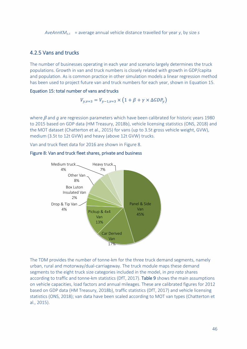
46

AveAnnKMy,s = average annual vehicle distance travelled for year y, by size s

4.2.5 Vans and trucks

The number of businesses operating in each year and scenario largely determines the truck populations. Growth in van and truck numbers is closely related with growth in GDP/capita and population. As is common practice in other simulation models a linear regression method has been used to project future van and truck numbers for each year, shown in Equation 15.

Equation 15: total number of vans and trucks

𝑉𝑦,𝑣=3 = 𝑉𝑦−1,𝑣=3 × (1 + 𝛽 + 𝛾 × ∆𝐺𝐷𝑃𝑦)

where and g are regression parameters which have been calibrated for historic years 1980 to 2015 based on GDP data (HM Treasury, 2018b), vehicle licensing statistics (ONS, 2018) and the MOT dataset (Chatterton et al., 2015) for vans (up to 3.5t gross vehicle weight, GVW), medium (3.5t to 12t GVW) and heavy (above 12t GVW) trucks.

Van and truck fleet data for 2016 are shown in Figure 8.

Figure 8: Van and truck fleet shares, private and business

The TDM provides the number of tonne-km for the three truck demand segments, namely urban, rural and motorway/dual-carriageway. The truck module maps these demand segments to the eight truck size categories included in the model, in pro rata shares according to traffic and tonne-km statistics (DfT, 2017). Table 9 shows the main assumptions on vehicle capacities, load factors and annual mileages. These are calibrated figures for 2012 based on GDP data (HM Treasury, 2018b), traffic statistics (DfT, 2017) and vehicle licensing statistics (ONS, 2018); van data have been scaled according to MOT van types (Chatterton et al., 2015).

Panel & Side Van45%

Car Derived Van17%

Pickup & 4x4 Van13%

Drop & Tip Van4%

Box Luton Insulated Van

2%

Other Van8%

Medium truck4%

Heavy truck7%

47

Table 9: The main truck and van model data and assumptions (1)


Average capacity (AvgCap), in tons/veh.

Average load (AvgLF)

Average annual distance travelled (AveAnnKM)

Constant

GDP coefficient g

Panel & side vans 0.8 36.6% 22,393 -0.0002088 0.9990167 Car derived vans 0.6 39.0% 20,197 -0.0002088 0.9990167 Pickup & 4x4 vans 0.8 36.6% 16,473 -0.0002088 0.9990167 Drop & tip vans 1.0 38.0% 18,970 -0.0002088 0.9990167 Box, Luton, ins. van 1.0 38.0% 24,377 -0.0002088 0.9990167 Other vans 1.0 35.1% 14,076 -0.0002088 0.9990167

Medium trucks 8.0 32.2% 73,796 -0.0205624 0.7167248 Heavy trucks 22.0 38.6% 49,260 -0.0110262 0.6534065

Notes: (1) the figures shown are for the year 2016. The reference scenario assumes some of these change over time.

These parameters feed into the calculation of total vehicle-km travelled by each truck size category, as shown in Equation 16.

Equation 16: Van and truck traffic by vehicle size category

𝑉𝐾𝑀𝑦,𝑣=3,𝑠 =𝑇𝐾𝑀𝑦,𝑣=3,𝑑


where: VKMy,v=3,s = vehicle-km for year y, by size s (6 van types, 2 HGV types)

PKMy,v=3,d = tonne-km for year y, by demand segment d

AvgCaps = average capacity (in tonnes per vehicle), by size s


The disaggregation of future road freight demand (in tonne-km, from TDM) to road freight vehicle types is an exogenous input to the model, simulating structural changes in vehicle logistics (and the expected transition from larger to smaller vehicles in urban areas). This is illustrated in Figure 9 which shows that HGVs, in particular larger trucks, transport the vast majority of freight by weight, while the van shares increase gradually over time. Amongst the latter, panel and side vans dominate tonne-km demand.

48

Figure 9: Projected changes in shares of total road freight demand by vehicle type

4.2.6 Passenger aircraft

Passenger aircraft are bought on a commercial basis in a highly competitive market. Any change in passenger numbers (trips) and destinations (trip lengths) will have a direct effect on total vehicle numbers. Aircraft numbers have therefore been assumed to depend on the ratio of the total annual vehicle kilometres (based on passenger-km from the TDM, which are divided by the average load factors from the scenario module) and the average number of kilometres per plane and year.

The TDM provides the number of passenger-km for domestic and international aviation. The aircraft module maps these demand segments to the five aircraft size categories included in the model, namely small jets (private/chartered), domestic short haul, international medium haul / Europe, international long haul / intercontinental and international supersonic (NB: the supersonic category is not used at present as all Concorde aircraft were retired in the early 2000s). Table 10 shows this mapping together with assumptions on vehicle capacities, load factors, the annual number of trips per aircraft and the average distance per aircraft per flight for the year 2015. These assumptions were derived from calibrating the model to national transport statistics (CAA, 2017; DfT, 2017). The reference scenario assumes that these input parameters stay constant over the modelling horizon. These assumptions can of course be modified for simulation of alternative scenarios such as changes in aircraft capacities and utilisations.

0

0.1

0.2

0.3

0.4

0.5

0.6

0.7

0.8

0.9

1

20

12

20

14

20

16

20

18

20

20

20

22

20

24

20

26

20

28

20

30

20

32

20

34

20

36

20

38

20

40

20

42

20

44

20

46

20

48

20

50

Heavy truck

Medium truck

Other vans

Box, Luton, ins. van

Drop & tip vans

Pickup & 4x4 vans

Car derived vans

Panel & side vans

49

Table 10: The main passenger aircraft demand modelling assumptions (1)

Demand segment

Aircraft size category

Average capacity (AvgCap), pass./plane


Average annual trips per aircraft (AvgAnnTrips)

Average distance per trip (AvgTripDist), km

Domestic Small jets 4 50% 531.0 250

Domestic Short distance

90 65% 510.3 500

International, medium haul / Europe

Medium distance

215 65% 1,422.3 2,100

International, long haul / intercontinental

Long distance

275 78% 726.1 5,475

International, supersonic (2)

Supersonic 100 76% 639 6,000

Notes: (1) the figures shown are for the year 2015. The reference scenario assumes that these parameters stay constant over the modelling horizon. (2) Not used currently.

Total vehicle-km travelled are derived for each aircraft size category according to Equation 17.

Equation 17: Aircraft traffic by size category



where: VKMy,v=4,s = vehicle-km for year y, by aircraft size s

PKMy,v=4,d = passenger-km for year y, by air demand segment d

AvgCaps = average capacity (in passengers per vehicle), by aircraft size s

AvgLFs = average load factor (in % of capacity), by aircraft size s

The total number of aircraft needed to fulfil demand is then derived by dividing total annual aircraft-km by the product of the average annual trips per aircraft and the average distance per aircraft and per trip, as shown in Equation 18.

Equation 18: Total aircraft numbers


𝐴𝑣𝑔𝐴𝑛𝑛𝑇𝑟𝑖𝑝𝑠𝑦,𝑠 × 𝐴𝑣𝑔𝑇𝑟𝑖𝑝𝐷𝑖𝑠𝑡𝑦,𝑠

50

where: Vy,v=4,s = vehicle stock for year y, by aircraft size s

VKMy,v=4,s = vehicle-km for year y, by aircraft size s

AvgAnnTripsy,s = average annual number of trips for year y, by size s

AvgTripDisty,s = average trip distance per aircraft for year y, by size s

4.2.7 Freight aircraft

Dedicated freight aircraft are also bought on a commercial basis in a highly competitive market. Any change in freight lifted and destinations (trip lengths) will have a direct effect on total vehicle numbers. As with the passenger aircraft module, freight aircraft numbers are assumed to depend on the ratio of the total annual vehicle kilometres (based on tonne-km from the TDM, which are divided by the average load factors from the scenario module) and the average number of kilometres per plane and year.

Domestic and international air freight demand is mapped onto the three freight aircraft size categories included in the model (Table 11). The reference scenario assumes that the input parameters shown in Table 11 stay constant over the modelling horizon. The parameter figures were derived from reviewing some of the literature and calibrating the model to national transport statistics (CAA, 2017; Chapman, 2007; DfT, 2017) for 2015. These assumptions can be modified for simulation of alternative scenarios.

Table 11: The main freight aircraft demand modelling assumptions (1)

Demand segment

Aircraft size category

Average capacity (AvgCap), tons/plane


Average annual trips per aircraft (AvgAnnTrips)

Average distance per trip (AvgTripDist), km

Domestic Short distance

18 60% 185 500

International, medium haul / Europe

Medium distance

35 65% 936 1,500

International, long haul / intercontinental

Long distance

90 65% 546 4,500

Notes: (1) the figures shown are for the year 2015. The reference scenario assumes that these parameters stay constant over the modelling horizon.

Total vehicle-km travelled and total vehicle stock are derived for each freight aircraft size category using Equation 17 and Equation 18, similar to the passenger aircraft model.

51

4.2.8 Passenger and freight trains

In contrast to other models, the number of new trains that will enter the population is determined by the national investment in motorised rail rolling stock (i.e. locomotives and motorised carriages). In TEAM this is achieved for each of the four passenger rail categories and the rail freight category shown in Table 4. The user has the option to alter this assumption for the testing of policies including, for example, large-scale investment in rail stock. Thus, the overall number of vehicles is calculated as the sum of previous vehicles, minus scrapped, plus new vehicles, as shown in Equation 19.

Equation 19: Total rail rolling stock

where

𝑁𝑉𝑦,𝑣 =𝐴𝑛𝑛𝑅𝑜𝑙𝑙𝑖𝑛𝑔𝑆𝑡𝑜𝑐𝑘𝐼𝑛𝑣𝑒𝑠𝑡𝑚𝑒𝑛𝑡𝑦,𝑣

𝐴𝑣𝑔𝑅𝑜𝑙𝑙𝑖𝑛𝑔𝑆𝑡𝑜𝑐𝑘𝑃𝑟𝑖𝑐𝑒𝑦,𝑣

Note with this approach it could easily happen that if investment were too low (and scrappage would continue at historic rate) total rail traction stock would decline over time, with the added effect that the average annual distance travelled by rail traction stock would increase (provided demand stays the same).

As for the calculation of total train-km, the TDM produces the number of passenger/tonne-km for four passenger rail categories and the rail freight category demand segments, which are mapped onto the appropriate train size categories (Table 12). Vehicle capacities, load factors and average rolling stock prices were derived from calibrating the model to national transport statistics (DfT, 2016, 2017), which also provide annual rolling stock investment for various segments of the national rail rolling stock.

Table 12: The main train demand model assumptions (data shown are for 2015)


Average capacity, pass./train or tons/train

Average load Average annual vehicle distance travelled

Average Rolling Stock Price, £million per train

Annual Rolling Stock Investment, £million

Light rail, underground

468 41.0% 67,041 2.5 78.8

Regional rail 250 43.2% 70,000 5.0 865.2

Intercity rail 447 45% 200,000 10 182.0

High speed rail 750 60% 275,000 20 65.0

Rail freight 380 70% 100,000 10 247.8

vyvyvyvy SVNVV ,1,1,, MvYy ,

52

These parameters feed into the calculation of total vehicle-km travelled by each train size category, as shown in Equation 20.

Equation 20: Train traffic by vehicle size category

𝑉𝐾𝑀𝑦,𝑣=5,𝑠 =𝑃𝑇𝐾𝑀𝑦,𝑣=5,𝑑


where: VKMy,v=5,s = vehicle-km for year y, by size s

PTKMy,v=5,d = passenger/tonne-km for year y, by demand segment d

AvgCaps = average capacity (in passengers/tons per vehicle), by size s


4.2.9 Freight shipping

In absence of any better data the number of freight ships in the vehicle population is assumed to remain constant, and new ships will enter the population only as replacements for ships that are scrapped (Equation 21). This is clearly a gross simplification, which could be modified as a later refinement of the VSM. The user has the option to alter this assumption for the testing of policies including, for example, large-scale investment in canal or port infrastructure.

Equation 21: Total shipping stock

𝑁𝑉𝑦,𝑣=6,𝑠 = 𝑆𝑦−1,𝑣=6,𝑠

where: NVy,v=6,s = new vehicle stock for year y, by ship size s

Sy-1,v=6,s = scrapped ship stock, by ship size s

The demand model provides projections of demand for three freight shipping demand segments (domestic inland, domestic coastal, international maritime), which are mapped onto the appropriate ship size categories (Table 13). The limited amount of appropriate data on ship capacities and load factors were based on UK domestic waterborne freight statistics (DfT, 2018a) and adjusted to TEAM categories to ensure internal consistency within the model. These parameters feed into the calculation of total vehicle-km travelled by each ship size category, as shown in Equation 20. Note international maritime statistics were not available across the parameters; therefore, maritime / international freight has not been included in this version of TEAM.

53

Table 13: The main shipping demand model assumptions (2015 data)

Vehicle size category Average capacity, tons/ship

Average load Average annual vehicle distance travelled

Inland / river 2,418 0.5 3,405 Coastal 23,200 0.5 18,575 Maritime / international 46,329 0.5 41,262

Equation 22: Shipping traffic by vehicle size category

𝑉𝐾𝑀𝑦,𝑣=6,𝑠 =𝑇𝐾𝑀𝑦,𝑣=6,𝑑


where: VKMy,v=6,s = vehicle-km for year y, by ship size s

TKMy,v=6,d = tonne-km for year y, by demand segment d

AvgCaps = average capacity (in tons per vehicle), by size s


4.3 Vehicle scrappage

4.3.1 Approach

Vehicles are scrapped at the end of their usable life. This can occur for the following reasons:

insurance ‘write-off’ following an accident;

bodywork deterioration beyond economic repair;

engine or other mechanical deterioration beyond economic repair;

voluntary scrappage due to price incentives;

prescribed scrappage due to legislation.

Cars

Within a saturated car market, where the number of cars per person remains constant (a state not yet reached in any market in the world), the rate of vehicle scrappage is crucial to the rate of deployment of new technologies. Within the UK car market, where rates of growth in car ownership are assumed to decline as saturation levels are approached, vehicle scrappage rates are extremely important in determining the turnover of technologies within the vehicle fleet.

With the improving build quality of modern vehicles, the average lifespan of vehicles may increase, decreasing stock turnover and slowing the introduction of new vehicle

54

technologies. Possible options for introducing new propulsion or emissions control technologies include replacing the engine, engine management systems and/or exhaust systems in older vehicles rather than scrapping them altogether when their propulsion technology fails or becomes obsolete. Other options include incentives for scrapping vehicles over a certain age (a.k.a. scrappage schemes, see e.g. Brand et al. (2013)). In addition, as tailpipe emissions from vehicles are reduced, the environmental impacts of vehicle construction and disposal will start to form a larger proportion of their overall life cycle impact – this is profound in the case of zero (tailpipe) emissions vehicles such as battery EVs. Encouraging longer lifespans could be a strategy for reducing this effect.

Other vehicles

For vehicles other than cars (particularly commercial vehicles) the life is more often determined in advance, and the investment in the vehicle is depreciated over a certain time period – usually four years. The expected resale value at that stage becomes an important factor. Scrappage of commercial vehicles takes place when they are considered “life expired” by their owners. This will be a commercial decision, based on the needs of the business, rather than (necessarily) because the vehicle can no longer perform a function at all. In many cases vehicles have a set life, over which they will be depreciated by the organisation that owns them. Once they are fully depreciated they may have some years of useful life left, or they may be scrapped to make way for a more modern vehicle that provides an improved level of service to the organisation.

To estimate the scrappage rate of vehicles a series of S-shaped life curves have been used in TEAM. These are somewhat different for each vehicle type (for example the average life of a train is far higher than that of a commercial truck). Apart from the vehicle type average life expectancy (probably the single largest explanatory factor), the average life expectancy might also be related to:

scrappage incentives;

inspection and maintenance standards;

investment policy (public transport);

safety requirements;

World trade levels (for shipping).

The variables used in TEAM for modelling vehicle scrappage are:

average vehicle lifespan;

financial incentives/disincentives for scrappage;

changing real price of vehicles.

4.3.2 Model specification

The decommissioning of vehicles from the vehicle stock due to scrappage is modelled using a modified Weibull distribution. The Weibull distribution is often used to model the likelihood of component failure with age (see e.g. de Jong et al., 2004).

55

The scrappage function is based on two parameters: failure steepness, which is the rate at which the likelihood of vehicles being scrapped increases with age, and the characteristic service life. The approach closely follows the FOREMOVE model (Zachariadis et al., 1995).

The calculation of scrappage of vehicles is carried out in the same manner for all vehicle types, but the scrappage parameters vary by vehicle type. The characteristic service life varies by technology and can be changed by the technical user to take account of policy options such as the introduction of long term scrappage incentives (that may or may not have an effect on average service lives) or, conversely, the encouragement of buying vehicles with a longer life (e.g. battery EVs).

The first function shown in Equation 23 provides the share of vehicles of a specific type v

that remain operating A years after first registration (i.e. A is the age of the vehicle). is a sigmoid function (S-shaped curve) defined by the failure steepness and the characteristic service life.

Equation 23: Modified Weibull distribution

where: Av,y = age of vehicle type v in year y

d = failure steepness for vehicle type v

g = characteristic service life for vehicle type v

The scrappage probability function can then be specified as a ratio of the share of vehicles of a specific age remaining in the current year to the share of vehicles one year younger being present in the population:

Equation 24: Scrappage probability function

where provides the probability of vehicles of each type and age to be scrapped in a

specific year (i.e. ).

This probability is finally multiplied by the number of vehicles present in the previous year to provide the total number of vehicles scrapped. This calculation is performed first for each vehicle type, age and year, and then filtered through to all vehicle technologies:

9f

9f

v

v

vyvA

kvay ef

,

9,,,

f

f

kva

kva

9,,1

9,,

1

10

56

The parameters used are dependent on the type of vehicle and the country, based on data used in the model described in FOREMOVE (Zachariadis et al., 1995). For the model to perform effectively (and for calibration of the parameters used) a detailed age breakdown of the fleet in the base year is required. National vehicle licensing statistics (DfT, 2009) were used to calibrate the UK figures for failure steepness and characteristic service life. The parameters are listed in Table 14 for the main vehicle types in TEAM.

Table 14: Scrappage parameters by vehicle type

Vehicle type Characteristic service life Failure steepness

Passenger vehicles

Motorcycle 14 5

Car 21 7

Bus & coach 25 7.5

Passenger train 40 10

Passenger aircraft 38 15

Freight vehicles

Panel & side vans 20 7

Car derived vans 21 7

Pickup & 4x4 vans 22 7

Drop & tip vans 20.5 7

Box, Luton, ins. van 20.5 7

Other vans 23 7

Medium and heavy trucks 15 5

Freight train 40 10

Ships 30 6.5

Freight aircraft 38 15

Source: scrappage parameters derived from UK Vehicle Licensing Statistics (ONS, 2018), with van type differentiation based on age distribution obtained from the MOT database (Chatterton et al., 2015).

The shapes of the sigmoid curves are illustrated for a selection of vehicle types in Figure 10. This shows that motorcycles and HGV live shorter ‘lives’ than, say, trains and planes.

GgZzAaMvYyVS gzvyagzvya ,,,,,,,1,1,,,,

57

Figure 10: Scrappage probability function for selection of vehicle types

Source: scrappage probability functions based on vehicle licensing data for the UK

4.4 Calculation of the total new vehicle stock

As already indicated earlier the number of new vehicles needed to enter the fleet in any given year is simply derived by taking the difference between the number calculated as remaining from the previous year (Vy-1 – Sy-1) and the total number of vehicles calculated to meet demand in the current year Vy (Equation 25). The number of vehicles remaining from the previous year is obtained as the difference between the vehicle stock of the previous year minus the vehicles scrapped at the end of the previous year.

Equation 25: Number of new vehicles needed

where represents the number of new vehicle needed for the current year y, and

represent, respectively, the vehicle stock of the current and the previous year and

represents the number of vehicles scrapped.

0%

10%

20%

30%

40%

50%

60%

70%

80%

90%

100%

0 5 10 15 20 25 30 35 40

scra

pp

age

pro

bab

ility

vehicle age

Cars

Motorcycles

Buses

Passenger rail

Aircraft

Panel and side vans

Pickup and 4x4 vans

Other vans

HGV

vyvyvyvy SVVNV ,1,1,, MvYy ,

yNV yV

1yV

1yS

58

Equation 25 is the same for each vehicle type and is applied for each year. Note, however

that for shipping vessels ( ) the assumption made is that (see above).

4.5 Disaggregation of the total number of new vehicles by size or type


The car model is the most disaggregated, with the new car fleet modelled by size/category (defined by three car types/sizes), ownership (private and fleet/company) and six consumer segments. This distinction makes it possible to simulate policies affecting different market (e.g. company car tax, scrappage rebate for private buyers) and consumer segments.

The new car market is first segmented into private and company/fleet markets, then into three vehicle segments according to the UK definitions of car segment and size (segments A/B – size ‘small’, C/D – ‘medium’, E/F/G/H – ‘large’) (SMMT, 2014). The same private consumer split applies across each vehicle segment, but the private/fleet sales split and annual mileages vary across vehicle segments. Using UK data to illustrate the segmentation, Figure 11a shows the sales by vehicle ownership and segment/size, highlighting the significance of the fleet/company market (52.5% of all new cars) (SMMT, 2018).

Figure 11: (a) Car market shares by vehicle ownership (private or fleet/company) and vehicle segment/size; (b) Car market shares by vehicle ownership (private or fleet/company) and consumer segment in the UK market (2015 data)

Source: Adapted from SMMT (2018) and ETI (ETI, 2013).

Notes: (a) Car segment and size are denoted by A/B – ‘small’, C/D – ‘medium’, and E/F/G/H – ‘large’. (a/b) Private car market denoted by blue patterned pie segments; fleet/company market denoted by green patterned pie segments. (b) Consumer segments denoted by four private and two fleet/company segments, with further details in Table 15 below. Percentage shares correspond to market shares for each segment.

6v 1 yy VV

Private

A/B, 26%

Private, C/D,

13%Private, E/H,

8%Fleet,

A/B, 15%

Fleet, C/D,

24%

Fleet,

E/H, 14%

(a)

Private, 'Enthusia

st', 7%Private,

'Aspirer', 7%

Private, 'Mass',

24%

Private, 'Resistor',

9%

Fleet, 'User

chooser', 20%

Fleet, 'Fleet

manager', 33%

(b)

59

Consumer acceptance, defined as the readiness to consider purchasing or using an alternative fueled vehicle (AFV), varies across consumers, with the majority of private consumers not accepting as sufficiently advanced the capability of current AFV models. For example, reliability, safety and battery degradation issues, as well as uncertainty regarding residual values, contribute to consumers’ reluctance to purchase BEVs. Building on the consumer study of 2,729 UK car buyers (Anable et al., 2016; Brand et al., 2017; ETI, 2013), the private buyer market was simplified from the eight segments found in Anable et al. (2016) into four segments and extended to include company-owned vehicles (Table 15 and Figure 11b). This takes into account that among company-owned cars, some are chosen by private individuals (termed ‘user-choosers’) – for whom the same purchase criteria as private cars apply – while the rest are selected by a decision maker within an organisation (‘fleet managers’) who generally have different decision making criteria than private buyers.

Table 15: Consumer segmentation across private and company/fleet markets

Private (47.5%)

‘Enthusiasts’ (15%)

Driven by innovativeness and prepared to pay a premium for AFVs. While they represent most of the early adopters of AFVs, they only account for a small fraction of car buyers

‘Aspirers’ (15%)

Interested in AFVs but concerned by their technical

limitations. AFV adoption by this group improves with the

increased availability of AFV models from trusted brands and the provision of market incentives that address both cost and technical barriers

‘Mass market’ (50%)

While AFV have no particular interest or symbolic meaning to this group, they are followers of social norms and are likely to become more receptive to AFV as their numbers increase

‘Resistors’ (20%)

Unlikely to buy AFVs as they strongly reject their symbolism (the perceived status and social acceptability of owning an AFV). This group’s receptiveness to AFVs will change only once AFVs have lost their current connotations, i.e. only once already widely adopted

Fleet/ company (52.5%)

‘User-choosers’ (38%)

Consider company-car ownership as primarily an individual purchasing behavior, hence utility calculations are similar to those for private buyers

‘Fleet managers’ (62%)

More likely to consider the total cost of ownership (TCO) and practical issues (such as technical suitability) and are less concerned with the brand and image

Note: Values in brackets show the UK segment size for the year 2015

The UK new car size split has been evolving slightly in favour of small and large cars, with small cars in segment A/B taking up around 41% of the market, medium (C/D) 27% and large (E+) 22%. Vehicle size split is a scenario input variable so can be changed for future years for sensitivity analysis or exploration of scenario variants, such as banning the sale of large (E+) cars from a specified date.

60


The new van and truck market is first segmented into private and business markets, then into eight vehicle segments. Six van types were developed for TEAM based on UK registration data obtained from the MOT tests and results database for 2012 (DfT, 2019). This database allowed us to model the private/business sales split and different annual mileages, energy use and emissions rates vary across vehicle segments (see Table 9).

Using UK data to illustrate the segmentation, Figure 12 shows van/truck market shares by vehicle ownership (a: private = 49.3%, b: business = 50.7%) and vehicle segment/size, highlighting the dominance of panel and side vans in both private and business markets. Vehicle size split is a scenario input variable so can be changed for future years for sensitivity analysis or exploration of scenario variants, such as taxing heavy trucks or banning the sale of larger vans from a specified date.

Figure 12: (a) Private van/truck market shares by vehicle segment/type; (b) Business van/truck market shares by vehicle segment in the UK (2015 data)

4.5.3 Other vehicle types

The ‘reference’ size distributions for new buses and ships are assumed to remain constant over the time horizon. In other words, the proportion of vehicles of each size obtained from the most recent statistics determines the split of sizes of new vehicles in each of the following modelled years. Crucially, size split is a scenario variable and can be modified by the user to simulate, say, ‘banning’ one vehicle size from entering the total vehicle fleet. Similarly, in a future where consumers prefer smaller cars over larger ones, the availability of large cars can be phased out over time.

The size distribution of new trains is dependent on the investment in rail rolling stock, which is disaggregated by vehicle size and a key policy input variable. So for example, if High Speed Rail 2 went ahead in earnest the UK would have to invest heavily in high speed rail rolling stock in the latter part of the period between 2015 and 2035.

Panel & side vans

45%

Car derived

vans20%

Pickup & 4x4 vans

18%

Drop & tip vans2%

Box, Luton, ins.

van1%

Other vans14%

Medium trucks

0%

Heavy trucks

0%

(a) private49.3%

Panel & side vans

45%

Car derived

vans14%

Pickup & 4x4 vans

9%

Drop & tip vans5%

Box, Luton,

ins. van3%

Other vans2%

Medium trucks

8%

Heavy trucks14%

(b) business50.7%

61

The approach for new aircraft stock assumes a constant size distribution of the aircraft fleet, identical with the size distribution obtained from the most recent statistics. Size split is a scenario variable and can be modified by the user. Within each size category, however, the user can change the capacity of aircraft. In one exogenous scenario of the TEAM, aircraft capacity is assumed to increase slowly over time while average load factors stay constant.

4.6 Vehicle technology availability

For each year a number of alternative vehicle technologies will be available in the market place, both for privately owned and commercial vehicles. The drivers of the availability of different technologies are:

make and model availability;

consumer demand;

legislation on fuel type, vehicle emissions, energy consumption, safety and noise;

differential taxation (by technology/fuel), on either fuel or vehicle;

technological breakthrough.

Different scenarios within TEAM clearly have different pathways of technological development. The default values developed here are included in the reference scenario. Note that any policies can of course alter these development pathways. All vehicle technologies have been specified in terms of technological and economic characteristics that are relevant to the modelling of vehicle technology choice, including:

propulsion technology (fuel type, hybridisation, vintage/innovation technology);

purchase price, purchase tax, vehicle road tax (VED in the UK);

fuel price and fuel tax;

(non fuel) operation and maintenance costs, e.g. fixed insurance and maintenance costs, depreciation costs for commercial vehicles;

other vehicle taxation such as Benefit-in-Kind (paid by private buyers of a company car) and national insurance contribution benefits (C1NIC) paid by the fleet manager/employer;

expected vehicle life (e.g., higher expected life for EVs?);

discount rate (private, fleet, commercial) for calculating annuities.

This module is common to both parts of the VSM (cars and other vehicles). It determines the vehicle technologies available in any given year, and contains the variables that describe the vehicles, to enable them to be selected through the vehicle choice modules.

The main technology characteristics used in the VSM are:

price excluding tax;

taxation levels (affected by policy users) for fuels, vehicle purchase, annual vehicle ownership, emissions levy or carbon tax;

62

costs of operation, per vehicle-km, including fuel used, road pricing charges, parking charges, pre tax fuel price.

Table A4 in Appendix A lists the 1246 vehicle technologies included in TEAM (v2.5), including first and last year of availability and the average purchase price.

4.7 Vehicle technology choice

The purpose of the technology choice module is to split the demand for new vehicles (in terms of numbers) among the different available technologies, for any specific vehicle type (such as medium-sized, C/D class cars, panel & side vans, urban buses or international middle range aircraft).

Technology choice is a complex decision making process, particularly with regard to the private consumer. The choices made by the private consumer are much less likely to be driven by business-focused types of considerations. To the private individual a car represents much more than a means of travelling from A to B. The individual is likely to buy the most expensive vehicle they can afford (i.e. they will set a capital budget at the outset of the choice process), and within that price range seek to satisfy a number of personal desires, ‘needs’ and ‘wants’.

In contrast, commercial organisations procure vehicles that will provide the best return on their investment. Thus they must balance the total lifetime benefits of a particular vehicle against the total lifetime cost. To model their decisions accurately it would therefore be necessary to model both the differences in benefits provided by different technologies, and also the differences in cost. However too little is known about the benefits side of this equation to provide a model of the way different organisations would assess marginally different technologies. Therefore a simplifying assumption was made, that the different technologies available for the same vehicle mode and size offer the same level of utility to the organisation - i.e. the only difference may lie in the expected costs of purchase, operation, maintenance and resale. In addition to costs, market availability, infrastructure availability, vehicle performance and technology preference of a commercial organisations have been included within a discrete choice modelling framework.


Car choice model – overview

The TEAM’s car choice model is a discrete choice model that estimates the purchase choice probability based on an assessment of overall vehicle ‘attractiveness’ (or ‘utility’) from amongst a set of vehicle choices (or ‘alternatives’), each with their own financial and non-financial ‘attributes’. The weighting of attributes varies across consumer segments, because consumers’ opinions on the importance of different vehicle attributes (e.g. running costs) vary. The model therefore reproduces the variation in utility of different vehicles across consumer segments, and the variation over time as vehicle attributes improve. Figure 13 gives an outline of the car choice model including key inputs and outputs.

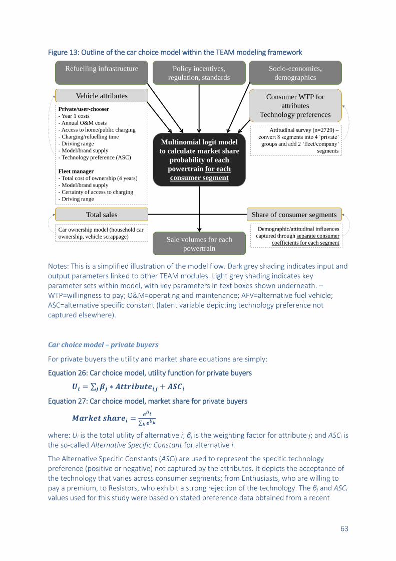
63

Figure 13: Outline of the car choice model within the TEAM modeling framework

Notes: This is a simplified illustration of the model flow. Dark grey shading indicates input and output parameters linked to other TEAM modules. Light grey shading indicates key parameter sets within model, with key parameters in text boxes shown underneath. – WTP=willingness to pay; O&M=operating and maintenance; AFV=alternative fuel vehicle; ASC=alternative specific constant (latent variable depicting technology preference not captured elsewhere).

Car choice model – private buyers

For private buyers the utility and market share equations are simply:

Equation 26: Car choice model, utility function for private buyers

𝑼𝒊 = ∑ 𝜷𝒋 ∗ 𝑨𝒕𝒕𝒓𝒊𝒃𝒖𝒕𝒆𝒊,𝒋 + 𝑨𝑺𝑪𝒊𝒋

Equation 27: Car choice model, market share for private buyers

𝑴𝒂𝒓𝒌𝒆𝒕 𝒔𝒉𝒂𝒓𝒆𝒊 =𝒆𝑼𝒊

∑ 𝒆𝑼𝒌𝒌

where: Ui is the total utility of alternative i; βj is the weighting factor for attribute j; and ASCi is the so-called Alternative Specific Constant for alternative i.

The Alternative Specific Constants (ASCi) are used to represent the specific technology preference (positive or negative) not captured by the attributes. It depicts the acceptance of the technology that varies across consumer segments; from Enthusiasts, who are willing to pay a premium, to Resistors, who exhibit a strong rejection of the technology. The βj and ASCi values used for this study were based on stated preference data obtained from a recent

Vehicle attributes Consumer WTP for

attributes

Technology preferences

Multinomial logit model

to calculate market share

probability of each

powertrain for each

consumer segment

Sale volumes for each

powertrain

Share of consumer segments

Refuelling infrastructure

Demographic/attitudinal influences

captured through separate consumer

coefficients for each segment

Private/user-chooser

- Year 1 costs

- Annual O&M costs

- Access to home/public charging

- Charging/refuelling time

- Driving range

- Model/brand supply

- Technology preference (ASC)

Fleet manager

- Total cost of ownership (4 years)

- Model/brand supply

- Certainty of access to charging

- Driving range

Car ownership model (household car

ownership, vehicle scrappage)

Policy incentives,

regulation, standards

Socio-economics,

demographics

Attitudinal survey (n=2729) –

convert 8 segments into 4 ‘private’

groups and add 2 ‘fleet/company’

segments

Total sales

64

consumer and vehicle choice study (Anable et al., 2016; Anable et al., 2011b; ETI, 2013) and given further below.

It should be noted that the consumer segments are only relevant to the UK market. Since attitudes to and technology preferences of EV technology may change significantly over time, the technology preference values revealed in 2011 may well change over the modelling horizon. We have therefore taken into account changes in preference values based on uptake rates and ‘consumer learning’, as explained further below.

Based on previous market research reported in Element Energy (2013) and Greene et al. (2014) the key vehicle attributes concerning private buyers were:

vehicle price;

running costs;

access to charging/refueling infrastructure;

charging/refueling time;

driving range;

model/brand supply, and;

consumer ‘receptiveness’ (i.e. technology preference).

Almost all of these attributes (the exceptions being running costs and access to overnight charging infrastructure) currently present a barrier to plug-in vehicle and other AFV adoption. All ‘enablers’ and ‘barriers’ were monetized, i.e. put on a ‘perceived’ basis; this does not mean that they represent actual costs. The choice model weighting factors βj were based on stated preferences of the choice experiment conducted for the ETI study (Anable et al., 2016; Element Energy, 2013). Table 16 summarizes the key attribute values and weighting factors for the Reference case.

Table 16: Vehicle attributes taken into consideration in the car choice model for private and fleet buyers

Attribute Value (reference case) – varies with time Weighting factors βj OR value of penalty – constant with time

Vehicle price

Price of vehicle + existing policy price signals (e.g. first year VED, plug-in vehicle grant, scrappage rebate), incl. VAT

Price coefficient (βj = Cp) based on revealed UK price elasticity: -0.0003521 for private consumers. ($),(1)

Running cost

Fuel costs (varies by fuel) + existing policy price signals (e.g. VED, BIK, ECA) + insurance and maintenance costs

The βj vary across consumer segments (Supplementary Material), from high weighting for ‘Enthusiasts’ (βj=7*Cp) to low weighting for ‘Resistors’ (βj=2*Cp). ($),(1)

Access to overnight charging

70% of private buyers have access to overnight off-street charging up to 2050. 25% of fleet buyers have certainty of access in 2015, rising to 40% by 2030

Overnight charging: pre-requisite for BEVs; Day charging: value of access for BEVs (£2,000) and 4 year fuel savings (variable) for PHEVs. (2)

65

Charging/ refuelling time

Average energy used for recharging (varies by fuel type, vehicle segment and hybridization) divided by power rate (e.g. BEV/PHEV: 3kW in 2015)

Based on stated preference, value of £250/h is assumed to decrease over time by taking the highest charging rate available to calculate the charging time. Charging time coefficient: -0.088025. (3)

Driving range

Real world range, varies by vehicle segment and powertrain, from 110km (BEV, 2015) increasing to 400km for large cars by 2030

Decreasing slope function of approx. £30/km, from approx. £3,000 at 150km to zero at ‘ideal range’ (from which there is no perceived penalty) at 370km. (3)

Model/ brand supply

Low supply, varies by vehicle segment and powertrain:

𝑃𝑒𝑛𝑎𝑙𝑡𝑦 = 𝟐𝟑⁄ ∗

ln(𝑠ℎ𝑎𝑟𝑒 𝑜𝑓 𝐴𝐹𝑉)

𝐶𝑝

Supply penalty is quantified as per the technique first developed by Greene in the U.S., i.e. based on the share of AFV models for sale. Values range between £0 (equal availability) to £10,484 (only 1 model available in medium size segment). (4)

Notes: ($) In line with the price elasticity reported in the Eftec (2008) and Tanaka et al. (2014) studies. Running cost coefficients are set to reproduce the willingness to pay (WTP) for running cost savings which differs for each consumer segment, see Supplementary Material S1. BIK = Benefit-In-Kind, graded by CO2, with tax payable by individuals with a fleet car (‘user-choosers’); VED = CO2-graded Vehicle Excise Duty (road tax); PC = price coefficient; ECA = Enhanced Capital Allowance, benefit to company in ‘fleet manager’ case.

Sources: (1) Eftec (2008); (2) Lin and Greene (2010) and Element Energy (2013); (3) Dimitropoulos (2011), Hidrue et al. (2011) and Stephens (Stephens, 2013); (4) Greene (1998; 2001).

The running cost coefficients are set to reproduce the willingness to pay (WTP) for running cost savings (Table 17). This varies from a WTP of £7 upfront to save £1 annual for ‘Enthusiasts’ to a WTP of only £2 for ‘Resistors’. This can be interpreted as ‘payback time horizon’: for a vehicle with a capital cost premium over the incumbent (gasoline internal combustion engine vehicle), the running costs savings must offset the premium over 7 years for ‘Enthusiasts’ (for the market share to reach 50% in the case of a comparison between two technologies). This time period is reduced to 2 years for ‘Resistors’. Another way to interpret the WTP for running cost savings is to translate them into discounting rates: the range is 7% for Enthusiasts to 48% for Resistors. The overall weighted average discounting rate of private buyers is 25%, which is in line with our previous work on this issue (Brand et al., 2013).

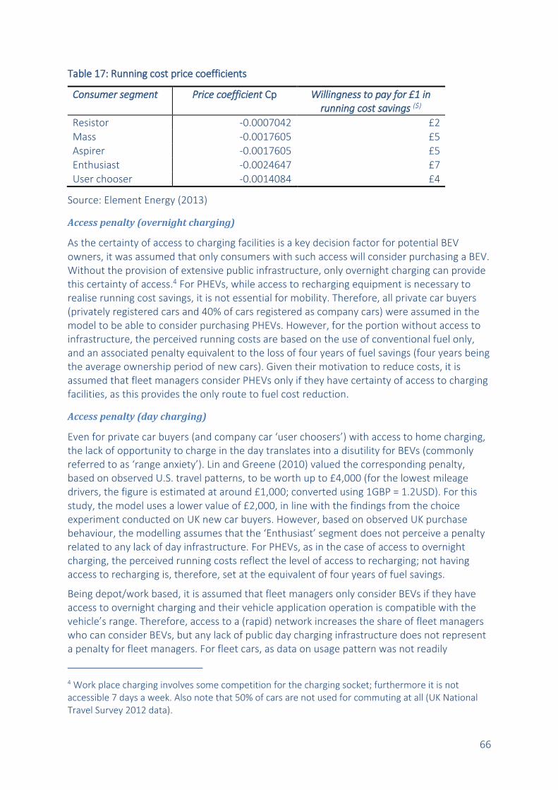
66

Table 17: Running cost price coefficients

Consumer segment Price coefficient Cp Willingness to pay for £1 in running cost savings ($)

Resistor -0.0007042 £2 Mass -0.0017605 £5 Aspirer -0.0017605 £5 Enthusiast -0.0024647 £7 User chooser -0.0014084 £4

Source: Element Energy (2013)

Access penalty (overnight charging)

As the certainty of access to charging facilities is a key decision factor for potential BEV owners, it was assumed that only consumers with such access will consider purchasing a BEV. Without the provision of extensive public infrastructure, only overnight charging can provide this certainty of access.4 For PHEVs, while access to recharging equipment is necessary to realise running cost savings, it is not essential for mobility. Therefore, all private car buyers (privately registered cars and 40% of cars registered as company cars) were assumed in the model to be able to consider purchasing PHEVs. However, for the portion without access to infrastructure, the perceived running costs are based on the use of conventional fuel only, and an associated penalty equivalent to the loss of four years of fuel savings (four years being the average ownership period of new cars). Given their motivation to reduce costs, it is assumed that fleet managers consider PHEVs only if they have certainty of access to charging facilities, as this provides the only route to fuel cost reduction.

Access penalty (day charging)

Even for private car buyers (and company car ‘user choosers’) with access to home charging, the lack of opportunity to charge in the day translates into a disutility for BEVs (commonly referred to as ‘range anxiety’). Lin and Greene (2010) valued the corresponding penalty, based on observed U.S. travel patterns, to be worth up to £4,000 (for the lowest mileage drivers, the figure is estimated at around £1,000; converted using 1GBP = 1.2USD). For this study, the model uses a lower value of £2,000, in line with the findings from the choice experiment conducted on UK new car buyers. However, based on observed UK purchase behaviour, the modelling assumes that the ‘Enthusiast’ segment does not perceive a penalty related to any lack of day infrastructure. For PHEVs, as in the case of access to overnight charging, the perceived running costs reflect the level of access to recharging; not having access to recharging is, therefore, set at the equivalent of four years of fuel savings.

Being depot/work based, it is assumed that fleet managers only consider BEVs if they have access to overnight charging and their vehicle application operation is compatible with the vehicle’s range. Therefore, access to a (rapid) network increases the share of fleet managers who can consider BEVs, but any lack of public day charging infrastructure does not represent a penalty for fleet managers. For fleet cars, as data on usage pattern was not readily

4 Work place charging involves some competition for the charging socket; furthermore it is not accessible 7 days a week. Also note that 50% of cars are not used for commuting at all (UK National Travel Survey 2012 data).

67

available, it was assumed that there is more variety in usage; as a result, range compatibility (before provision of day infrastructure) was set to 30% in 2020 and 40% in 2030.

Driving range penalty

Dimitropoulos et al. (2011) reported an average value for EV range of £30/km. This means consumers would be willing to pay £3,000 to add 100 km to the driving range of a BEV. Alternatively, if the maximum range of a BEV is 100 km less than the ideal range consumers would like, the range penalty is valued as £3,000. The incremental value of range decreases as the maximum range increases. In this study, this decrease in penalty was reproduced (from £30/km at 150 km), assuming that the ‘ideal range’ of 370 km was the limit over which no more penalty is perceived (i.e. value of driving range penalty over 370 km was zero).

Alternative specific constants

Further to attribute values and weighting factors provided in Table 16, the ASCi (technology preference) values used in this study were based on regression analysis of the empirical data (attitudinal survey and choice experiment) obtained from the ETI segmentation study (Anable et al., 2016) as reported in Element Energy (2013). Table 18 shows the monetized and normalized ASCi for plug-in vehicles for private and ‘user-chooser’ consumer segments.5 The data show that all attitudinal segments consider PHEVs more favorably than BEVs due to the performance characteristics of the respective technologies, and there is no clear bias towards owning a PIV as a second car in the household (Anable et al., 2016). Mass market buyers strongly reject BEVs but not PHEVs (as much).

We modelled ‘consumer learning’ and the neighbor effect by assuming that the technology bias encapsulated in the technology preference parameter (ASCi) decreased linearly with increasing sales from 100% of the ASCi value at no sales to 0% when sales reach 25% and above. (This modeling behaviour can be switched on or off for sensitivity analysis; the user interface provides a handy switch on the Run Model form.)

5 ASC values were monetized using the revealed UK price elasticity for private consumers Cp = -0.0003521, and normalized against the ‘Aspirer’ consumer segment. The conversion was done by dividing the utility term by the price coefficient.

68

Table 18: Default technology preference (ASCi) values for plug-in vehicles

Consumer segment Technology i ASCi ($) Perceived cost (+)

(in GBP)

Resistor PHEV -4.436 12,600 Resistor BEV -9.436 26,800 Mass PHEV -1.338 3,800 Mass BEV -5.282 15,000 Aspirer PHEV 0 0 Aspirer BEV 0 0 Enthusiast PHEV 1.373 -3,900 Enthusiast BEV 0.986 -2,800 User chooser PHEV -1.338 3,800 User chooser BEV -5.282 15,000

Notes: (+) Perceived cost values were derived from the ASCs using the revealed UK price elasticity of -0.0003521 for private consumers. ($) ASC and perceived cost values were normalized against the ‘Aspirer’ consumer segment.

Sources: Hidrue et al. (2011); Hoen and Koetse (2012); Batterbee and Lidstone (2013); Element Energy (2013).

Car choice model – fleet manager segment

In contrast to private buyers, fleet managers are assumed to approach potential vehicle purchase based on a rational assessment of TCO (Total Cost of Ownership), model/brand supply and technology suitability (charging access, driving range compatibility). Equation 26 simplifies to:

Equation 28: Car choice model, utility function for fleet manager segment

𝑼𝒊 = 𝜶 ∗ 𝑻𝑪𝑶𝒊 + 𝜷 ∗ 𝑺𝑷𝒊

where: Ui is the total utility of alternative i; TCO is the total cost of ownership over 4 years; α is the price coefficient for TCO (varies by vehicle segment); and β is the price coefficient for supply penalty SPi. The TCO includes depreciation costs (capital cost - resale value of 40% * discount factor, at a 10% discount rate) and 4-year running costs (discounted, including existing company/fleet car price signals).

The price coefficients for the ‘fleet manager’ consumer segments were derived from the elasticity in demand as per Greene et al. (2004). They vary by vehicle segment and are provided in Table 19.

Table 19: Baseline price coefficients for fleet managers (based on 2012 ICE cars)

Number of makes/models in each segment

TCO (£GBP) Average market share

Price elasticity ($)

Implied price coefficient

Small (A/B) 75 14,433 0.013 -15.71 -0.001103 Medium (C/D) 98 22,461 0.010 -15.71 -0.000707 Large (E to I) 255 33,397 0.004 -15.71 -0.000472

Source: Element Energy (2013), Greene et al. (2004)

69

Notes: ($) The elasticity is based on the willingness to pay data of fleet manager as collected during primary research reported in Element Energy (2013). This is higher than the price elasticities reported in, for example, Greene et al. (2004), reflecting the higher price sensitivity (and highly elastic demand) of the UK fleet manager market.

Car choice model – decision process

The choice model takes into account two important pre-conditions to be met for AFVs to be part of the choice set.

1. First, all buyers must be aware of AFVs and their incentives. The reference case assumes a sigmoid increase in awareness from low (10%) to moderate (50%) levels by 2030; this can be changed for scenario analysis.

2. Second, private buyers must have access to overnight charging (for BEV and HFCV) – this is assumed to stay constant at 70% over the time horizon. Also, fleet buyers must have certainty of access to charging/refueling and the range must meet the duty cycle requirement, in consistence with their technical suitability approach. For BEV, for instance, the reference case assumes low deployment of a rapid charging network so that only 25% of fleet buyers meet the range compatibility condition in 2015, rising to 40% by 2030 and then staying constant.

The decision process and choice model are run for each vehicle segment and consumer segment, with the share of vehicle and consumer segments being kept constant in the Reference case.


Van and truck choice model – overview

The van and truck technology choice model is similar if somewhat simpler than the car model. Again it is based on a discrete choice model that estimates the purchase choice probability based on an assessment of overall vehicle ‘attractiveness’ (or ‘utility’) from amongst a set of vehicle choices (or ‘alternatives’), each with their own financial and non-financial ‘attributes’. The weighting of attributes varies across consumer segments (private, business), because consumers’ opinions on the importance of different vehicle attributes (e.g. running costs) vary. The model therefore reproduces the variation in utility of different vehicles across consumer segments, and the variation over time as vehicle attributes improve. Figure 14 gives an outline of the van and truck choice model including key inputs and outputs.

70

Figure 14: Outline of the van and truck choice model within the TEAM modeling framework

Notes: This is a simplified illustration of the model flow. Dark grey shading indicates input and output parameters linked to other TEAM modules. Light grey shading indicates parameter sets within model, with parameters in text boxes shown underneath. – WTP=willingness to pay; O&M=operating and maintenance.

Van and truck choice model – private buyers

For private buyers the utility and market share equations are simply:

Equation 29: Van and truck choice model, utility function for private buyers

𝑼𝒊 = ∑ 𝜷𝒋 ∗ 𝑨𝒕𝒕𝒓𝒊𝒃𝒖𝒕𝒆𝒊,𝒋𝒋

Equation 30: Van and truck choice model, market share for private buyers

𝑴𝒂𝒓𝒌𝒆𝒕 𝒔𝒉𝒂𝒓𝒆𝒊 =𝒆𝑼𝒊

∑ 𝒆𝑼𝒌𝒌

where: Ui is the total utility of alternative i; βj is the weighting factor for attribute j.

It should be noted that the buyer segments may only be relevant to the UK market. Since technology preferences of AFV technology may change significantly over time, the technology preference values revealed in 2011 may well change over the modelling horizon. We have therefore taken into account changes in preference values based on uptake rates and ‘buyer learning’, as explained further below.

As with cars, and based on market research reported in Element Energy (2013) and Greene et al. (2014) the key vehicle attributes concerning private buyers were: vehicle price; running costs; access to charging/refueling infrastructure; charging/refueling time; driving range;

Vehicle attributes Consumer WTP for attributes

Multinomial logit modelto calculate market share

probability of each powertrain for both buyer

segments

Sale volumes for each powertrain

Share of buyer segments

Refuelling infrastructure

Socio-economic influences captured through separate buyer coefficients

for both segments

Private buyer (vans only)- Year 1 costs- Annual O&M costs- Access to home/public charging- Charging/refuelling time - Driving range- Model/brand supply

Business/fleet buyer- Total cost of ownership (4 years)- Model/brand supply- Certainty of access to charging- Charging/refuelling time- Driving range

Van/truck ownership model (road freight supply & demand, scrappage)

Policy incentives, regulation, standards

Socio-economics, demographics

Buyer survey of cars and vans, plus intel from MOT database produced

two segments for vans:Private and business/fleet

Total sales

71

model/brand supply; and consumer ‘receptiveness’ (i.e. technology preference). Almost all of these attributes (the exceptions being running costs and access to overnight charging infrastructure) currently present a barrier to plug-in vehicle and other AFV adoption. All ‘enablers’ and ‘barriers’ were monetized, i.e. put on a ‘perceived’ basis; this does not mean that they represent actual costs.

The βj coefficients used for TEAM were based on stated preference data obtained from a recent consumer and vehicle choice study (Anable et al., 2016; Anable et al., 2011b; Element Energy, 2013; ETI, 2013). Table 20 summarizes the key attribute values and weighting factors for the Reference case.

Table 20: Vehicle attributes taken into consideration in the van and truck choice model for private and fleet buyers

Attribute Value (reference case) – varies with time Weighting factors βj OR value of penalty – constant with time

Vehicle price

Price of vehicle + existing policy price signals (e.g. first year VED, plug-in vehicle grant, scrappage rebate), incl. VAT for private buyers

Price coefficient (βj = Cp) based on revealed UK price elasticity: -0.0003521 for private consumers. ($),(1)

Running cost

Fuel costs (varies by fuel) + existing policy price signals (e.g. VED, BIK for private, VED, C1ANIC for business buyers) + insurance and maintenance costs

The βj vary across consumer segments (Supplementary Material), from high weighting for ‘Enthusiasts’ (βj=7*Cp) to low weighting for ‘Resistors’ (βj=2*Cp). ($),(1)

Access to overnight charging

70% of private buyers have access to overnight off-street charging up to 2050. 22% of fleet buyers have certainty of access in 2012, rising to 40% by 2030, then staying constant

Overnight charging: pre-requisite for BEVs. Day charging: value of access for BEVs (£2,000) and 4 year fuel savings (variable) for PHEVs. (2)

Charging/ refuelling time

Average energy used for recharging by van/truck type, fuel type and hybridization (e.g. 60 and 6.6 kWh for BEV and PHEV vans) divided by power rate (e.g. BEV/PHEV: 3kW ‘home charging’)

Based on stated preference, value of £250/h is assumed to decrease over time by taking the highest charging rate available to calculate the charging time. Charging time coefficient: -0.088025. (3)

Driving range

Real world range, varies by vehicle segment and powertrain, from 220km (BEV vans, Euro 5) increasing over time to 400km for BEV vans (by 2025) and medium BEV trucks (by 2035)

Decreasing slope function of approx. £30/km, from approx. £3,000 at 150km to zero at ‘ideal range’ (from which there is no perceived penalty) at 370km. (3)

Model/ brand supply

Low supply, varies by vehicle segment and powertrain:

𝑃𝑒𝑛𝑎𝑙𝑡𝑦 = 𝟐𝟑⁄ ∗

ln(𝑠ℎ𝑎𝑟𝑒 𝑜𝑓 𝐴𝐹𝑉)

𝐶𝑝

Supply penalty is quantified as per the technique first developed by Greene in the U.S., i.e. based on the share of AFV models for sale in each segment. Values range between £0 (equal availability) to £6,837 (only 1 out of 37 models available as BEV in panel van segment). (4)

72

Notes: ($) In line with the price elasticity reported in the Eftec (2008) and Tanaka et al. (2014) studies. Running cost coefficients are set to reproduce the willingness to pay (WTP) for running cost savings. BIK = Benefit-In-Kind, graded by CO2, with tax payable by private buyers; VED = CO2-graded Vehicle Excise Duty (road tax); PC = price coefficient; C1ANIC = class 1A national insurance contribution, paid by business buyers.

Sources: (1) Eftec (2008); (2) Lin and Greene (2010) and Element Energy (2013); (3) Dimitropoulos (2011), Hidrue et al. (2011) and Stephens (Stephens, 2013); (4) Greene (1998; 2001).

The running cost coefficient for private van buyers is meant to reproduce the willingness to pay (WTP) for running cost savings. The coefficient for vans was based on the ‘user-chooser’ car segment with a value of -0.0014084 (Anable et al., 2016; Element Energy, 2013). Assuming a price coefficient for private buyers of -0.00035210 (see car choice model above), the van coefficient equates to a WTP of £4 upfront to save £1 annually. This can be interpreted as ‘payback time horizon’: for a vehicle with a capital cost premium over the incumbent, the running cost savings must offset the premium over 4 years (for the market share to reach 50% in the case of a comparison between two technologies, with everything else equal). Another way to interpret the WTP for running cost savings is to translate them into a discounting rate. This comes out at about 25%, which is in line with our previous work on this issue (Brand et al., 2013).

EV charging access penalty

In terms of access to overnight charging, all private van/truck buyers were assumed in the model to be able to consider purchasing PHEVs. For PHEVs the perceived running costs reflect the level of access to recharging; not having access to recharging is, therefore, set at the equivalent of four years of fuel savings. The value of access to overnight charging was £3,000 for BEVs, £3,750 for hydrogen FCVs and 4-year fuel savings (variable, between £3,000 and £4,120) for PHEVs.

Given their motivation to reduce costs, it is assumed that business/fleet buyers consider PHEVs only if they have 100% certainty of access to charging facilities, as this provides the only route to fuel cost reduction.

In terms of access to day charging, even for private van buyers with access to home charging, the lack of opportunity to charge in the day translates into a disutility for BEVs (commonly referred to as ‘range anxiety’). Lin and Greene (2010) valued the corresponding penalty, based on observed U.S. travel patterns, to be worth up to £4,000 (for the lowest mileage drivers, the figure is estimated at around £1,000; converted using 1GBP = 1.2USD). The reference case in TEAM uses a mid-range value of £3,000, in line with the findings from the choice experiment conducted on UK new van buyers (Element Energy, 2013) and the observation that vans travel more miles than cars. For PHEVs, as in the case of access to overnight charging, the perceived running costs reflect the level of access to recharging; not having access to recharging is, therefore, set at the equivalent of four years of fuel savings.

Being depot/work based, it is assumed that business/fleet buyers only consider BEVs if they have access to overnight charging and their vehicle application operation is compatible with the vehicle’s range. Therefore, access to a (rapid) network increases the share of fleet managers who can consider BEVs, but any lack of public day charging infrastructure does not

73

represent a penalty for business/fleet buyers. For business vans and trucks, as data on usage patterns was not readily available, it was assumed that there is more variety in usage; as a result, range compatibility (before provision of day charging infrastructure) was set to 25% in 2015, rising to 40% in 2030 then staying constant. This is a scenario variable, so higher (or lower) range compatibility values can be set to test future expansions of day charging networks.

Van and truck choice model – business/fleet buyer segment

In contrast to private buyers, business/fleet buyers are assumed to approach potential vehicle purchase based on a quasi-rational assessment of TCO (Total Cost of Ownership), model/brand supply and technology suitability (charging access, driving range compatibility):

Equation 31: Van and truck choice model, utility function for business/fleet buyer segment

𝑼𝒊 = 𝜶 ∗ 𝑻𝑪𝑶𝒊 + 𝜷 ∗ 𝑺𝑷𝒊

where: Ui is the total utility of alternative i; TCO is the total cost of ownership over 4 years; α is the price coefficient for TCO (varies by vehicle type); and β is the price coefficient for supply penalty SPi. The TCO includes depreciation costs (capital cost - resale value of 30% * discount factor, at a 10% discount rate) and 4-year running costs (discounted, including existing business vehicle price signals).

The price coefficients for the business/fleet buyer segment were derived from the elasticity in demand as per Greene et al. (2004). They vary by vehicle segment and are provided in Table 21.

Table 21: Baseline price coefficients α for business buyers (based on 2015 diesel vehicles)

Number of makes/models in each segment

TCO (£GBP) Marginal market share

Price elasticity ($)

Implied price coefficient α

Panel & side vans 37 49,969 0.027 -12.39 -0.0002549 Car derived vans 37 47,328 0.027 -12.39 -0.0002691 Pickup & 4x4 vans 20 48,405 0.050 -12.39 -0.0002695 Drop & tip vans 20 49,587 0.050 -12.39 -0.0002630 Box, Luton, insulated vans 15 52,171 0.067 -12.39 -0.0002545 Other vans 20 47,140 0.050 -12.39 -0.0002767 Medium trucks 25 179,481 0.040 -12.39 -0.0000719 Heavy trucks 25 279,222 0.040 -12.39 -0.0000462

Source: Element Energy (2013), Greene et al. (2004) and own calculations

Notes: ($) The elasticity is based on the willingness to pay data of business/fleet buyers as collected during primary research reported in Element Energy (2013). This is higher than the price elasticities reported in, for example, Greene et al. (2004), reflecting the higher price sensitivity (and highly elastic demand) of the UK business/fleet buyer market.

Van and truck choice model – decision process

The choice model takes into account two important pre-conditions to be met for AFVs to be part of the choice set.

74

1. First, all buyers must be aware of AFVs and their incentives. The reference case assumes a sigmoid increase in awareness from low (10%) to moderate (50%) levels by 2030; this can be changed for scenario analysis.

2. Second, private buyers must have access to overnight charging (for BEV and HFCV) – this is assumed to stay constant at 70% over the time horizon.

3. Third, business/fleet buyers must have certainty of access to charging/refueling and the range must meet the duty cycle requirement, consistent with their technical suitability approach. For BEV, for instance, the reference case assumes low deployment of a rapid charging network so that only 25% of business/fleet buyers meet the range compatibility condition in 2015, rising to 40% by 2030 and then staying constant.

The decision process and choice model are run for each vehicle type (e.g. panel and side van, medium truck) and buyer segment (private, business), with the share of vehicle and buyer segments being kept constant in the Reference case.

4.7.3 Other vehicle types: motorbikes, buses, trains, shipping vessels, aircraft

For all other vehicle types, the choice model is somewhat simplified. A vehicle of technology i (see Appendix A) is chosen with probability (probi) which is related to cost and non-cost factors of the vehicle using that technology. Cost factors are simulated by calculating the equivalent annual cost EACi for each technology i. Non-cost factors are simulated by a preference and performance parameter, Pi, which is an aggregate function of perceived performance (perf), market presence (pres) and consumer preference (pref) of the vehicle technology. From the mathematical point of view, the probability is modelled as a linear function of the preference and performance parameter and a multinomial logit function (commonly used in behavioural modelling, see e.g. Train, 2009) of the cost factors, as shown in Equation 32.

Equation 32: Technology choice probability function

m

j j

j

j

i

ii

i

EAC

EACcP

EAC

EACcP

prob

1 minexp

minexp

with

iiii prefpresperfP

where Pi = preference and performance parameter for vehicle technology i EACi = equivalent annual cost of vehicle technology i c = modelling constant (preset value of c=10 used for model calibrations) m = number of vehicle technologies available in modelling year perfi = perceived performance of vehicle technology i presi = market presence at maturity of vehicle technology i prefi = consumer preference for vehicle technology i

75

The price and non-price factors underpinning Equation 32 are described in more detail as follows.

Price Factors

The equivalent annual cost EACi is the cost per year of owning and operating a vehicle over its entire (economic) lifespan (Equation 33). It is the sum of the annuity of owning the vehicle over its economic lifetime and any annual operating and maintenance costs (e.g. fuel, road user charging, circulation taxes, insurance, maintenance and depreciation) to the consumer or operator. The annuity represents the annual payment of paying off a loan for all up-front costs (purchase price, purchase taxes and rebates). The applied discount (or interest) rate can vary by vehicle type (car, van, aircraft, etc.) and, to avoid a purely static approach, by year. Implicitly the EAC can vary by scenario (e.g. via changes in pre-tax fuel price) and policy (via e.g. changes in fuel duty).6

Equation 33: Annual cost of ownership and operation

𝐸𝐴𝐶𝑖 = −𝑃𝑀𝑇(𝐷𝑅𝑎𝑡𝑒𝑖, 𝐴𝑣𝑔𝐸𝑐𝑜𝑛𝐿𝑖𝑓𝑒𝑖 , 𝐼𝑛𝑣𝐶𝑜𝑠𝑡𝑖) + 𝐴𝑛𝑛𝐹𝑖𝑥𝐶𝑜𝑠𝑡𝑖 + 𝐴𝑛𝑛𝑉𝑎𝑟𝐶𝑜𝑠𝑡𝑖

where: EACi = equivalent annual cost of owning a vehicle of technology i PMT() = the payment for an annuity DRatei = discount (or interest) rate for technology i AvgEconLifei = average economic lifetime of vehicle technology i InvCosti = net investment or upfront cost of owning a vehicle technology i AnnFixCosti = annual fixed costs AnnVarCosti = annual variable costs.

Net ownership costs are simply the vehicle purchase price (after tax, incentives, rebates, etc.) calculated as an annuity over the economic lifetime of the vehicle. Fixed costs are costs of insurance, maintenance, depreciation, VED, etc. Variable costs are mainly determined by fuel costs, plus variable taxes such as road pricing and congestion charges. Specifically, annual fuel costs are calculated according to Equation 34.

Equation 34: Annual fuel costs

𝐴𝑛𝑛𝐹𝑢𝑒𝑙𝐶𝑜𝑠𝑡𝑦,𝑖 = (𝑅𝑒𝑠𝐶𝑜𝑠𝑡𝑦,𝑖 + 𝐹𝑢𝑒𝑙𝐷𝑢𝑡𝑦𝑦,𝑖) × 𝑉𝐴𝑇 × 𝑆𝐹𝐶𝑖 × 𝐴𝑣𝑒𝐴𝑛𝑛𝐾𝑀𝑦,𝑖

where: AnnFuelCosty,i = estimated annual fuel costs for technology i ResCosty,i = pre-tax fuel price for technology i FuelDutyy,i = transport fuel duty for technology i VAT = Value Added Tax rate (e.g. 1.2 for current 20% UK VAT rate) SFCi = specific fuel consumption for technology i, in litres per 100km AveAnnKMy,i = average annual distance travelled per vehicle technology i

6 EACi is also the basis for calculating relative transport costs (RC in Equation 1) which feeds back from the VSM to the TDM.

76

To populate the model, and to ensure that the full spectrum of the vehicle range is reflected in the purchase decisions, a detailed price distribution is needed. The variables needed for such an approach are:

Distribution of vehicles purchased, by annuitized lifetime cost (by year);

Purchase price of the new vehicle, including any taxes imposed (by year, vehicle type, size, engine type, fuel type);

Running costs of the new vehicle, based on:

o fuel price, with tax;

o annual taxes such as vehicle excise duty (VED);

o insurance and maintenance costs;

o any other charges imposed by the policy maker (e.g. parking charges, road pricing differentiated by technology);

o average annual mileage (by technology);

Average vehicle life (by technology).

The key variables are specified in the vehicle technology tables, summarised in Appendix A. The default discount rate for commercial buyers of planes, ships and so on was assumed to be 10%, simulating lower cost of capital and investment risk than for private buyers of, say, cars and motorbikes.

Non-price Factors

The P factor is an aggregate of three key factors that can influence purchasing decisions, based on market research by the UK Energy Saving Trust (2008). First, the factor of perceived performance perf is an aggregate of perceived safety and security, speed, acceleration, range between refuelling, space available and comfort. Secondly, the market presence factor pres represents the potential market presence of the vehicle technology at market maturity, including factors such as availability of and access to fuel as well as market coverage (i.e. is the technology widely available across the different market segments such as ‘super mini’, ‘small family’, executive’ and ‘multi-purpose vehicles’?). Thirdly, the consumer preference factor pref simulates non-cost factors that cannot be explained by cost, performance and market factors, e.g. vehicle colour, style and ‘technology loyalty’.

The obvious challenge of defining P has been approached in two different ways. First, in the case where the vehicle technology is an established one, with a consolidated market share such as gasoline and diesel cars, P can be derived using Equation 32 on the basis of observed, historical data such as the UK’s Vehicle Licensing Statistics (ONS, 2018). Since the values of P are not constant, but could change over time, it is necessary to verify their trends on the basis of observed data. In TEAM, this verification process was performed for the base year and subsequent modelling years where licensing statistics exist (from 2012 to 2016).

Secondly, for new and alternative vehicle technologies, neither cost nor preference and performance data are well established or can be observed directly. In addition, both cost and non-cost factors may change more radically in future years than for their conventional counterparts. Costs may decrease as production achieves economies of scale, technological developments cut intrinsic costs and vehicle life increases. Similarly, vehicle performance

77

may increase as technological developments improve utility and public perceptions change. Perceptions will be influenced by information such as marketing and technology demonstration, and also by the number of vehicles already in use. Market potentials may increase by the market providing larger ranges of models across the vehicle classes (e.g. fully electric buses may in future be available more widely across the market segments). Thus for each new and alternative vehicle technology the change in P over time is modelled as an S-curve using a logistic function (Note: this is distinct from the S-curve of market penetration, i.e. vehicle numbers.).

We assume that the new technology improves from a market entry year Tentry to a product maturity year Tmaturity, reaching a maximum level P at maturity (Figure 15). Tentry is defined as the entry year for the first commercially available vehicles (albeit these may also be regarded as commercial prototypes, likely to be used primarily in demonstration projects). Tmaturity is the year when the vehicle technology performance and consumer preference are expected to level off (or at least become parallel with the trend line for conventional technologies).7 P is estimated based on the expected relative market share of the new vehicle technology (in terms of new vehicle sales) in year T2, compared to some specified conventional comparator, that might be anticipated if the annualised costs of the conventional and new technologies were the same. Figure 15 illustrates this by showing four hypothetical curves comparing an existing reference technology to three new vehicle technologies with three different entry years, maturity years and levels of preference and performance.

Figure 15: Comparison of four hypothetical preference and performance parameter curves, other vehicle types (motorcycles, buses, trains, ships, aircraft, etc.)

7 Note Tmaturity is not the date when market penetration (share of new vehicle sales) levels off for the new technology. Growth in new vehicle sales may lag behind the rise in P, as the number of sales will also be critically dependent on differences in technology costs and taxes.

0

20

40

60

80

100

120

140

160

2008 2010 2012 2014 2016 2018 2020 2022 2024 2026 2028 2030

rela

tiv

e p

refe

ren

ce a

nd

perfo

rm

an

ce existing technology

future technology 1

future technology 2

future technology 3

P2

P1

P3

Tentry 2 Tentry 3 Tmaturity 3Tmaturity 1 Tmaturity 2

78

Notes: P = preference and performance at market maturity; Tentry = expected entry year for the first commercially available vehicles; Tmaturity = expected maturity year i.e. year when the preference for and performance of the new vehicle technology are expected to level off (or at least become parallel with the trend line for existing technologies).

Vehicle technology 1 represents a rather slowly progressing conventional technology where market entry happened in the past and maturity is expected in 2015, e.g. an urban HEV bus. Vehicle technologies 2 and 3 represent future technologies (with market entries of 2013 and 2019), with comparatively faster rates and at maturity higher expected performance and preference than technology 1. Technology 3 takes only 6 years to mature and even outstrips the reference technology.

Clearly the specification of future vehicle costs and P parameter curves are crucial to the medium to long term outcomes of the vehicle technology choice module. While default values for cost and non-cost parameters have been developed based on best available knowledge in the literature and in consultation with policy and industry experts, TEAM users can modify them according to their market expectations or for simple ‘what-if’ analysis.

The set of P parameters, Tentry and Tmaturity for the reference scenario are given in Appendix A.

4.7.4 Technology distribution of the new vehicle fleet

Taking the total number of new vehicles from Equation 25, the technology distribution of new vehicles is simply derived using Equation 35.

Equation 35: Distribution of new vehicles by technology

𝑁𝑉𝑡,𝑦,𝐴=0 = 𝑁𝑉𝑦,𝐴=0 × 𝑝𝑟𝑜𝑏𝑡,𝑦,𝐴=0

for all years y, technologies t that are available in that year, and age A = 0 (i.e. new).

4.8 Main outputs and links to other models

4.8.1 Vehicle fleet distributions

This module first combines the remaining vehicle population (disaggregated by vehicle age, size and technology) with the new vehicle population (disaggregated by size and technology) to provide a total population distribution, in each year (disaggregated by vehicle age, size and technology). The output tables are large in size, containing typically around 40 to 80 thousand records for a single scenario run. Table 22 shows the number of new (N), scrapped (S) and total (T) vehicles for technology ID 322 (i.e. “Road - Car - Medium - Gasoline – ‘Euro 7’ (2020-24) – Passenger Transport – Hybrid EV”) for policy package ‘REF’, exogenous scenario ‘CC’, region ‘UK’ and year 2024. The vehicle distributions are exported to the DEEM and LCEIM.

Table 22: Sample entry in output table Interface_VSM_NumVeh

Policy package

Scenario Region Year Technology Vehicle Category

Number of Vehicles

... ... ... ... ... ... ...

REF CC UK 2024 322 New 54,732

79

REF CC UK 2024 322 Scrapped 24,532

REF CC UK 2024 322 Total 675,501

... ... ... ... ... ... ...

4.8.2 Vehicle traffic distributions

The final stage of the vehicle supply model provides one of the three main outputs required for calculating emissions levels, namely the total vehicle-kilometres disaggregated by vehicle type, year, age, size, engine type and fuel type. In its current version, the model takes the vehicle-kilometres computed by vehicle type and journey segment type (e.g. urban car travel) from the TDM and splits each vehicle type according to the proportion of vehicle stock of that vehicle type in each technology category, modified to take account of factors such as age and technology. For cars it is known that the distribution of vehicle-km by age is skewed towards newer cars (ONS, 2007). The basic pro rata formula is shown in Equation 36.

Equation 36: Vehicle-km distribution by technology, vehicle type, size, fuel type and age

𝑉𝐾𝑀𝑦,𝑡,𝑣,𝑠,𝑎,𝑓𝑡 = 𝑉𝐾𝑀𝑦,𝑣,𝑠 ×𝑉𝑦,𝑡,𝑣,𝑠

𝑉𝑦,𝑣,𝑠

where: VKM = vehicle-km V = total number of vehicles

y = year t = technology v = vehicle type s = vehicle size

The relationship between car age and mileage is taken into account using an age, size and fuel type dependent scaling factor, as shown in Equation 37. The annual percentage change in mileage as car ages is assumed to be between 2.8% p.a. (small gasoline cars) and 5.7% p.a. (medium diesel cars) in the reference case (Figure 16). The model normalises to the total vehicle-km before final outputs are written to the database.

Equation 37: Car vehicle-km distribution by technology and age

𝑉𝐾𝑀𝑦,𝑡,𝑣=2,𝑠,𝑎 = (1 + 𝜀 × (𝐴𝑣𝑒𝐸𝑐𝑜𝑛𝐿𝑖𝑓𝑒𝑣=2,𝑦

2− 𝑉𝑒ℎ𝐴𝑔𝑒𝑦,𝑡,𝑣=2,𝑎)) × 𝑉𝐾𝑀𝑦,𝑣=2,𝑠

×𝑉𝑦,𝑡,𝑣=2,𝑠

𝑉𝑦,𝑣=2,𝑠

where: VKM = vehicle-km e = annual percentage change in mileage as car ages AveEconLife = characteristic vehicle service life

y = year t = technology v = vehicle type (v=2 is cars only) a = vehicle age (0=new, 1 year old, …, 40 years old) s = vehicle size

80

Figure 16: Scaling factor for simulating fuel, size and age dependence of car vehicle-km

4.8.3 Feedback to TDM – changes in generalised costs by mode of transport

Ownership and operating and maintenance costs of vehicles affect the ‘generalised travel costs’ that are traditionally used to determine modal split and journey distances in demand modelling.

The choices of vehicle technologies, taxation changes, and other related costs of supplying a passenger-km or tonne-km, are fed back into the mode choice model to affect the modal split. As presented earlier these generalised costs are computed as the relative change compared to the previous modelling year of the average annual transport costs per passenger/tonne-km (RC in Equation 1), weighted over the vehicle-km driven each year. For instance, increasing the fuel costs for 50% of the car fleet by 5% will increase the average-weighted transport costs by 2.5%, resulting in a relative cost factor of 1.025. If there is no cost increase for motorcycle, bus, rail and domestic air, the model will calculate (a) a reduction in total passenger transport demand and (b) modal shift from car to the other modes based on assumed cross elasticities.

0

0.5

1

1.5

2

2.5

0 2 4 6 8 10 12 14 16 18 20 22 24 26 28 30 32 34 36 38 40

scal

ing

fact

or

vehicle age

Small A/B - Gasoline Small A/B - Diesel Medium C/D - Gasoline

Medium C/D - Diesel Large E-H - Gasoline Large E-H - Diesel

81

5. Direct Energy and Emissions Model

5.1 Overview

The TDM and VSM provide vehicle-kilometres and average trip lengths, disaggregated by passenger/freight, vehicle type, size, propulsion technology and ‘route segment types’ (such as urban, rural and motorway for road, urban/light and high speed for rail, and take-off and cruise for air). From this, the DEEM calculates direct (i.e. tailpipe, at source) fuel and energy consumption as well as carbon and regulated air quality pollutant emissions arising from the operation of vehicles by using the established emissions factor method. Apart from direct energy use, the emissions types included in the DEEM are the direct greenhouse gases (GHG) carbon dioxide (CO2) and methane (CH4) as well as the indirect GHG carbon monoxide (CO), sulphur dioxide (SO2), nitrogen oxides (NOX), non-methane volatile organic compounds (NMVOC) and particulates (PM).8 Further pollutants are covered in the life cycle and environmental impacts model (Chapter 6).

The DEEM is able to model the combined effects of different fleet compositions, different sets of emission factors, traffic characteristics, cold starts, fuel quality and driver behaviour. The DEEM interfaces with other modelling components in TEAM as illustrated in Figure 17.

Figure 17: Interfacing of the DEEM and TNM models within TEAM

8 Nitrous oxide (N2O), the other direct GHG, is accounted for in the LCEIM.

TNM DEEM

TDM / Traffic Demand & Vehicle Stock Models

EIM

Direct Energy & Emission Model

Traffic Noise Model

Environmental Impact Model

VSM

82

5.2 Model specification, data sources and calibration

The basis for all calculations of energy consumption and exhaust emission are disaggregate sets of emission factors (e-factors) based on the results of large scale vehicle emissions testing programmes. For road transport, speed distributions for each vehicle type (car, motorcycle, van, HGV) and route segment type (urban, rural, motorway) are used to calculate the energy consumption and emissions, based on average speed-emissions curves developed in previous research and emissions inventories such as COPERT (EEA, 1998, 2000, 2012, 2017), MEET (Hickman et al., 1999), HBEFA (Chen and Borken-Kleefeld, 2014; INFRAS, 2004, 2009) and NAEI (NETCEN, 2003). These datasets provide a base set of emissions factors (mostly for conventional ICE and some HEV vehicle technologies), which is mapped onto TEAM vehicle technologies and then scaled for future technologies – thus providing the default set of emissions factors for TEAM. The user can change both mapping and scaling to simulate effects of policy such as fuel efficiency standards.

Emissions factors for road vehicles at normal operating temperatures (often called ‘hot’) are a polynomial function of average speed, with up to ten coefficients for each pollutant. The TEAM base emissions factors are based on HBEFA (INFRAS, 2004, 2009) coefficients, which were originally calibrated in extensive vehicle emissions testing. The road transport module also takes account of cold start effects. Cold start emissions mainly depend on ambient temperatures and trip distances.

The default speed distributions are based on observed data for Great Britain (DfT, 2014a, b, c). To take account of effects such as congestion and speed limits the user can alter the speed distributions.

For all other modes, average emissions factors are used to calculate energy use and emissions. For air, emissions factors are split into the different flight stages ‘landing/take-off’ (LTO) and ‘cruise’. The share of the LTO phase compared to the total flight distance is estimated based on the international CORINAIR/SNAP classification (code 08 05), where the flight distance up to an altitude of 1000 metres – about 30 km –is allocated to airport traffic.

5.2.1 Functional linkages for road transport

The dependencies of variables are outlined in two schematic overviews. First, Figure 18 shows the functional linkages for calculating road traffic volumes. Secondly, Figure 19 illustrates the main functional linkages for calculating energy consumption and exhaust emissions for road transport.

83

Figure 18: Schematic overview of the functional linkages for road traffic

Notes: ‘fl’ stands for mileage; IO = urban traffic, AO = rural traffic, BAB = motorway and dual carriageway traffic; NV = local traffic, FV = long distance traffic

stock

mileage [Km/a]

fl = 1.E-6 * stock * mileage [Mio Km/a]

%fl_NV

%fl_NV_IO

%fl_NV_AO

%fl_NV_BAB = 100 - (%fl_NV_IO + %fl_NV_AO)

fl_NV = fl * %fl_NV * 0.01 [Mio Km/a]

fl_IO = (fl_NV * %fl_NV_IO + fl_FV * %fl_FV_IO) [Mio Km/a]

%fl_FV = 100 - %fl_NV

%fl_FV_IO

%fl_FV_AO

%fl_FV_BAB = 100 - (%fl_FV_IO + %fl_FV_AO)

fl_FV = fl * %fl_FV * 0.01 [Mio Km/a]

fl_AO = (fl_NV * %fl_NV_AO + fl_FV * %fl_FV_AO) [Mio Km/a]

fl_BAB = (fl_NV * %fl_NV_BAB + fl_FV * %fl_FV_BAB) [Mio Km/a]

link to next diagraminput variable computed variable

84

Figure 19: Schematic overview of the functional linkages for energy consumption and exhaust emissions from road transport

Notes: ‘fl’ stands for mileage; IO = urban traffic, AO = rural traffic, BAB = motorway and dual carriageway traffic; NV = local traffic, FV = long distance traffic; MJ = Megajoule, PJ = Petajoule; ‘vm’ stands for ‘mean velocity’ or ‘average speed’

5.2.2 Speed-emissions curves

The speed dependence of ‘hot’ e-factors for all road vehicle types is managed by polynomial regression up to a maximum degree of 9th order, as shown in Equation 38.

85

Equation 38: Dependence of energy use and emissions on average speed

9

9,,

2

2,,1,,0,,, *** jjijjijjijiji ScScSccEF

where EFi,j = energy use or emissions factor for pollutant i and vehicle type j Sj = average speed for vehicle type j ci,j,x = polynomial coefficients (x=0,…,9) for pollutant i and vehicle type j

As mentioned above all emissions factors used in TEAM are based on a set of base or primary emissions factors which are parameterised according to Equation 38. An example is shown in Figure 20.

Figure 20: View and edit ‘base’ emissions factors in DEEM

Note: PKW (“Personenkraftwagen”) = passenger car; selected base technology is ‘PKW1DKE3’ = passenger car, small size (A/B segment), diesel (primary fuel), EURO 3 standard. UKTCM=UK Transport Carbon Model.

Examples of the resultant speed emissions curves are shown in Figure 21 for two medium sized petrol car technologies (conventional ICE and hybrid electric EV). The somewhat flatter curve at lower average speeds for HEV cars is a result of better fuel economy and CO2 emissions at lower, urban speeds.

86

Figure 21: Base speed-emissions curves for fuel use and NOX emissions for small petrol cars

Note for non-road modes of transport (air, rail, shipping) speed independent e-factors are used. This implies that only the constants (coefficients c0) are used in the above equation.

5.2.3 Speed profiles

The other key component in the methodology is the use of speed profiles disaggregated by vehicle type and road type (urban, rural, motorway/dual carriageway). The default speed profiles are based on observed distributions of average (as opposed to free flow) traffic speeds, which in the UK case were taken from GB national statistics (DfT, 2014a, b, c). The default or reference scenario speed profiles are given in Appendix B and illustrated in Figure 22.

More than half of all cars travel on motorways at speeds higher than the current speed limit (70 mph). Alternative speed profiles for cars on motorways/dual carriageways have been developed for policy analysis, e.g. limiting or increasing the speed limit or better enforcement of existing laws (Anable and Brand, 2011). Figure 23 shows one alternative scenario for cars on motorways/double carriageways. The blue distribution represents currently observed data; the red distribution represents one possible distribution if the speed limit would be enforced more effectively.

87

Figure 22: Reference road speed profiles for cars, buses and trucks

Source: Road traffic speed distribution (DfT, 2014a, c)

Figure 23: Example speed profiles for cars on motorways/double carriageways

Source: Road traffic speed distribution (DfT, 2014a, c), and own assumptions for enforced speed limits.

5.2.4 Integration

By using scaling factors and cross-referencing between ‘base’ and ‘actual’ e-factor databases (as illustrated in Figure 24 and Figure 25) the DEEM can handle any new technology the policy maker may wish to examine. If the ‘base’ vehicle technology did not exist it can be added and specified in terms of speed emissions characteristics (ideally the full functional relationship between mean speed and ‘hot’ and cold start emissions).

Car Urban

Car Rural

Car Motorway

Bus Urban

Bus Rural

Bus Motorway

Trucks Urban

Trucks Rural

Trucks Motorway

pe

rce

nta

ge o

f ve

hic

le-k

m

trav

ell

ed

wit

hin

b

rack

et

average speed brackets (km/hr)

0-10

10-20

20-30

0%

5%

10%

15%

20%

25%

30%

35%

speed brackets [km/hr]

speed profiles for cars

car, motorway, existing speed limits

car, motorway, speed limits enforced

88

Figure 24: Cross referencing and scaling of energy use and emissions factor datasets in the TEAM

Figure 25: Variable linkages for modelling energy consumption and emissions

Notes: sf = scaling factor; v_5-15 indicates share of vehicle traffic in speed bracket ‘5-15 kph’; efp = emissions factor (primary emissions type i.e. fuel use, CO2, etc.); ‘warm’ and ‘cold’ stand for ‘hot’ and ‘excess cold’ emissions factors respectively; pct = percentage.

Figure 26 provides average fuel consumption factors (in grams of fuel per vehicle-km) for a range of gasoline car technologies at average speed 50 kph, disaggregated by propulsion technology (ICE, HEV, PHEV) and vintage (EURO 4, 5, 6, etc). This set of factors represents only a fraction of the vehicle technologies currently modelled in TEAM. Similar figures exist for other vehicle types and technologies.

Stock oftechnologies

Crossreference

scalingfactors

Base e-factortablesef(v)

Velocitydistribution

pct(v)

1:1 n:1

convolution

Mean specificenergy consumption& & emission

exhaust

89

Figure 26: Fuel consumption for petrol cars at 50 kph average speed

0 10 20 30 40 50 60

Road - P - CAR - Small - Gasoline (petrol) - Conventional (no catalyst) - vintage 1980 to 1992

Road - P - CAR - Small - Gasoline (petrol) - Euro 1 (incl. catalyst) - vintage 1992 to 1996




Road - P - CAR - Small - Gasoline (petrol) - Euro 5 (2009-14) - vintage 2009 to 2015








Road - P - CAR - Small - Gasoline (petrol) - Euro 5 (2009-14) - PHEV - vintage 2009 to 2015








Road - P - CAR - Medium - Gasoline (petrol) - Conventional (no catalyst) - vintage 1980 to 1992

Road - P - CAR - Medium - Gasoline (petrol) - Euro 1 (incl. catalyst) - vintage 1992 to 1996




Road - P - CAR - Medium - Gasoline (petrol) - Euro 5 (2009-14) - vintage 2009 to 2015








Road - P - CAR - Medium - Gasoline (petrol) - Euro 4 (incl. catalyst) - HEV - vintage 2005 to 2010

Road - P - CAR - Medium - Gasoline (petrol) - Euro 5 (2009-14) - HEV - vintage 2009 to 2015








Road - P - CAR - Medium - Gasoline (petrol) - Euro 5 (2009-14) - PHEV - vintage 2009 to 2015








Road - P - CAR - Large - Gasoline (petrol) - Conventional (no catalyst) - vintage 1980 to 1992

Road - P - CAR - Large - Gasoline (petrol) - Euro 1 (incl. catalyst) - vintage 1992 to 1996




Road - P - CAR - Large - Gasoline (petrol) - Euro 5 (2009-14) - vintage 2009 to 2015








Road - P - CAR - Large - Gasoline (petrol) - Euro 4 (incl. catalyst) - HEV - vintage 2005 to 2010

Road - P - CAR - Large - Gasoline (petrol) - Euro 5 (2009-14) - HEV - vintage 2009 to 2015








Road - P - CAR - Large - Gasoline (petrol) - Euro 5 (2009-14) - PHEV - vintage 2009 to 2015








Fuel consumption (grams of fuel per km) for petrol cars at 50 kph average speed, by technology

90

5.3 Scenario and policy modelling in the DEEM

The DEEM is able to model scenario and policy options relating to:

Improved fuels with lower content of key pollutants (CO2, NOX, PM2.5, NMVOC)

Speed and congestion modelling

Driver behaviour

Cold start influence

Any time dependency of e-factors.

This functionality has been implemented by incorporating into the modelling chain a complex set of scaling factors which are applied to the calibrated TEAM fuel use and emissions factors from the previous Section.

For instance, in order to model alternative scenarios/policies that affect average speeds and levels of congestion the user has the option to define alternative speed profiles. Congestion can be modelled at the national level by shifting the distribution to lower speed brackets. While speed profiles are defined by vehicle type and road type, all technologies belonging to the specified class of vehicle types are affected by the settings. Figure 27 shows a screenshot of the user forms relevant to speed/congestion modelling in DEEM.

Figure 27: Screenshot of the DEEM user forms for speed/congestion modelling

Changes in driver behaviour can be simulated by applying a set of scaling factors that allow to consider how specific emissions change (in this case decrease) over time as a result of, say, a national eco-driving programmes (Figure 28).

91

Figure 28: User set up for driver behaviour change

5.4 Model calibration

As the methodologies used in the DEEM differ slightly from those used to derive national statistics and accounts, the DEEM needs to be calibrated at the levels of travel demand, traffic and energy use and emissions to national statistics for each year between the base year (i.e. 2012 in this version) up to the most recent year where a full set of stats are available (usually two years prior to the current year). This can be done by applying scaling factors in table EF_timebehav to the DEEM energy use and emissions factors shown above. A couple of SQL queries have been setup in the TEAM user interface database for exactly this purpose.

92

6. Life Cycle and Environmental Impacts Model

6.1 Approach

As far as the transport sector is concerned the basic principle of life cycle analysis (LCA) is to take into account all relevant up- and downstream processes within a defined system boundary. Based on a typical environmental life cycle assessment framework (Holland et al., 2016; ICO, 2006; Rabl and Holland, 2008), the Life Cycle and Environmental Impacts Model (LCEIM) comprises:

1. A life cycle inventory model, and;

2. An environmental impacts assessment model.

The life cycle inventory model calculates indirect energy use and emissions (including primary energy and land use) for:

the manufacture, maintenance and disposal of vehicles;

the construction, maintenance, and disposal of infrastructure, and;

the supply of energy (fuels).

The environmental impacts assessment model then provides an assessment of the damage caused by calculating impact indicators (e.g. global warming potential, GWP) and external costs.

The life cycle inventory model uses the ‘hybrid approach’ of process-chain analysis and input-output analysis developed by Marheineke et al. (1998; 1996; Strømman et al., 2009). Process chain analysis is used for the main supply paths, and aggregated values for complete process chains are used within the model. For additional upstream processes, considered to be second or third-order effects, input-output analysis is used. This hybrid approach is seen as appropriate as much of the evidence in the literature suggests that, in most cases, over the lifetime of a vehicle, vehicle operation produces the vast majority of energy use and GHG emissions (Lane, 2006; MacLean and Lave, 2003). While for conventional vehicles the fuel supply and vehicle manufacture stages account for about 20% of total lifetime GHG emissions – being roughly equal in magnitude – vehicle maintenance and disposal account for a much smaller share (ibid.). Of course, EVs, H2FCVs and biofuel-powered vehicles have different shares of emissions, with the majority of EV and H2FCV emissions coming from vehicle manufacture and generation of electricity/hydrogen.

The environmental impacts assessment model converts direct (from the DEEM) and indirect (from the life cycle inventory model) emissions into impacts, which include a number of common impact indicators and external costs. Impact indicators are a means to describe environmental damage and to compare different pollutants with respect to a certain impact using different weighting factors. For example, the GWP100 (100-year Global Warming Potential) describes the warming impact of emissions over the next 100 years, and the POCP (Photochemical Ozone Creation Potential) refers to the formation of photochemical oxidants. The methodology for determining external costs is based on an evaluation of marginal effects. To estimate marginal effects an Impact Pathway Approach has been used, building on

93

previous research on the European ExternE project and subsequent studies (Bickel et al., 2003; EC, 2005; Holland et al., 2018; Rabl et al., 2014).

The LCEIM allows the user to simulate the effects on energy use and emissions of e.g. adding new infrastructure (e.g. high speed rail), changes in the electricity generation mix and an alternative set of impact potentials (IPCC, 2018: for current climate change impact potentials).

6.2 What the user can and ‘should not’ change

There are six parameter sets in the current version of the LCEIM that may be edited/defined by the user. For all other life cycle or environmental impact data, user access is not recommended. This is due to the fact that most of the model data inputs are generated elsewhere in the modelling chain. Hence, it is simply not possible for the user to define their own data at this point, since the user data would not be consistent with other model data.

The parameters that the user can edit/define via the graphical user interface (Figure 29) of the TEAM are:

additional transport infrastructure including high speed rail lines, roads and airports (this parameter will exclusively be defined by the user; there are no default/reference data for this parameter);

future electricity generation mixes (in 10 year intervals to 2100);

accident costs (monetary values for fatalities, minor and serious casualties);

average accident rates (fatalities, minor and serious casualties);

impact potentials (e.g. GWP100 figures for CH4 and N2O; HCA figures for NOX and PM2.5), and;

population density for spatial demand segments (urban | motorway | intercity rail | etc.).

Figure 29: LCEIM user interface, definition of model alternatives and policies

94

In addition the user has the option to change the default data sets that are internal to the LCEIM and that were produced off-line using separate databases and/or by using other models. These include:

indirect emissions, primary energy demand and land use change for the production, maintenance, and scrappage of vehicles;

indirect emissions, primary energy demand and land use for the construction, maintenance, and disposal of infrastructure;

energy use and emissions factors for electricity generation by generation technology;

indirect emissions, primary energy demand and land use for the production and supply of all 15 fuels considered in TEAM;

the VOC-split of exhaust emissions from conventional and alternative fuelled vehicles, and;

external cost and monetary valuation rates for the various impact categories, accidents and pollutant and noise emissions.

6.3 Modelling methodology

6.3.1 Life Cycle Inventory Model

The necessary data sets for LCA such as emission factors for the provision of materials and the provision of energy carriers are modelled in TEAM as aggregated values for an entire process chain. The LCEIM is directly connected in terms of data flow (i.e. interface databases) to the VSM, the DEEM and the TEAM User Interface, as illustrated in Figure 30.

Figure 30: Life Cycle Inventory Model Linkages

TEAM-EIM

TEAM-LCM

95

Vehicle Manufacture, Maintenance and Scrappage

Life cycle analysis of vehicles includes the manufacture, maintenance and scrappage of vehicles. The preceding TEAM component models feed into the LCA model, which converts technology ownership and use data (i.e. number of vehicles) to LCA data (i.e. mass of materials needed). The calculation of indirect emissions from the manufacture, maintenance and disposal of vehicles follows two main steps:

1. First, each vehicle type (e.g. medium sized internal combustion car) is broken down into its components in terms of mass of materials needed to manufacture the vehicle and for vehicle maintenance (e.g. tyres, lubricants etc.). At present over 15 materials are modelled for each vehicle type, including alkyd resin varnish, aluminium, glass, polypropylene, rubber and three types of steel. Based on the material decomposition, emissions, primary energy use and land use changes embedded in each kg of material are derived, for up to 25 emissions categories including embedded CO2, N2O, ‘land use conversion from undeveloped to cultivated’ (in metre square/kilogram of material) and ‘crude oil’ (in kilogram of oil/kilogram of material).

2. Secondly, the energy use and emissions for the processes involved in manufacturing, maintenance and disposal are derived by multiplying energy requirements for each process category with process emissions factors.

For step one, for example, the embedded CO2 emissions factors for unalloyed, low-alloy and high-alloy steel are 1.61, 1.97 and 5.28 kg of CO2 per kg of material respectively. For aluminium this is even higher at 9.97 kg of CO2 per kg of material.

To perform this conversion the technologies considered in TEAM needed to be classified by mass category (essentially vehicle size) and by material category. Two different categories are used since two technologies may be of different weight but have the same percentage of materials. The disaggregation level of the mass classification of vehicles is such that all types of vehicles are clearly distinguished concerning emissions and energy demand for vehicle manufacture. The disaggregation level of the material structure of vehicles is such that all main components of vehicles are considered, including the battery for EVs.

Another crucial point is the temporal system boundary for life cycle analysis of vehicles – temporal with regards to the vehicle fleet which is subject to evolution and continuous change. New vehicles are added and old vehicles are scrapped. Although energy requirements and emissions related to the manufacture of a vehicle can be seen as values that should be distributed over the whole lifetime of the vehicles, TEAM allocates all manufacturing emissions to the year of first registration. This was deemed the most feasible method for the following reasons:

Independent modelling of a certain year will be possible.

A direct evaluation of new technologies is possible as all effects (including LCA) are considered in one year and it is not necessary to compare discounted values over a time horizon of about 10 years.

Infrastructure Construction and Maintenance

Data availability or data procurement is a fundamental issue concerning infrastructure construction and maintenance. Detailed infrastructure modelling would require an infrastructure-demand model to consider the following effects:

96

changes in infrastructure may have a considerable influence on congestion;

heavy duty vehicles for example cause by far more damage to roads than cars;

a higher transport demand does not necessarily lead to new infrastructure.

However, appropriate data and an infrastructure demand model were not available. Hence the modelling of these effects was deemed to be beyond the scope of TEAM. Nevertheless, it is desirable for TEAM to allow an analysis of significant changes in modal split or the introduction of new transport technologies (such as a High Speed Train network). To consider this, the user has the option to specify any additional infrastructure to the existing infrastructure network. Although modelled separately, the relevant LCEIM assumptions on additional infrastructure need to be consistent with the assumptions made in the TDM.

The calculation of indirect emissions for the construction, maintenance and disposal of additional infrastructure follows the same methodology as for life cycle assessment of vehicles. The underlying data are based on a number of life cycle studies, where available based on UK context, including more generic inventories on fuels and powertrains (Brinkman et al., 2005; DTI, 2000; JEC, 2014; Joint Research Centre, 2006) and vehicle manufacturing and disposal (Lane, 2006; Schäfer et al., 2006; Zamel and Li, 2006) as well as more specific ones on vehicle materials (International Iron and Steel Institute, 2002), infrastructure materials (e.g. cement, Nemuth and Kreißig, 2007) and process emissions (e.g. freight transport, Höpfner et al., 2007).

The allocation of emissions from additional infrastructure is weighted by vehicle-km, which presents a simplification as, for example, heavy duty vehicles (doing fewer miles than cars overall) are responsible for a much larger share of the damage. Double counting within the hybrid life cycle inventory was avoided as much as possible following Strømman et al. (2009).

In addition to energy consumption and emissions caused by infrastructure construction the corresponding land use impacts are derived as an impact indicator.

Fuel and Energy Supply

Emissions from fuel and energy supply are calculated by converting energy and fuel use provided by the DEEM into emissions using well-to-tank emissions factors. The fuels and energy carriers covered are:

Gasoline (petrol) and advanced gasoline,

Diesel (DERV) and advanced diesel,

LPG (liquefied petroleum gas),

Bio-ethanol petrol blend (E85),

Bio-diesel (from woody biomass) (B100),

CNG (compressed natural gas),

Electricity,

GH2 (gaseous hydrogen),

LH2 (liquid hydrogen),

Kerosene (Jet-A aviation fuel) and

Bio-kerosene.

The fuel supply emission factors used in the life cycle inventory model are pre-determined based on an extensive literature review (Brinkman et al., 2005; Frischknecht et al., 1997; JEC,

97

2014; JRC and CONCAWE EUCAR, 2006). For example, the indirect CO2 emissions factors for the above fuels are provided in Table 23 below.

Table 23: Transport fuel specifications and indirect CO2 emissions factors from fuel supply

Fuel type Embedded CO2

Unit Density (kg/litre)

Cal. Value (MJ/litre)

Gasoline (petrol) 540 kg/ton 0.75 32.18 Diesel (DERV) 612 kg/ton 0.83 35.86 Liquefied Petrol Gas 400 kg/ton 0.54 24.80 Bioethanol-petrol blend (E85) -15108 kg/TJ 0.79 29.26 Biodiesel (B100) 2nd gen. -55930 kg/TJ 0.89 33.11 Compressed Natural Gas (1) 5170 kg/TJ 0.16 7.72 Compressed Bio Gas (1) -38490 kg/TJ 0.16 7.72 Gaseous Hydrogen (2) 8000 kg/TJ 0.06 7.00

Liquefied Hydrogen (3) 552 kg/ton 0.08 9.20 Aviation fuel (BP Jet A-1) 561 kg/ton 0.80 34.69 Bio jet fuel (100%) -55930 kg/TJ 0.79 34.00

Notes: (1) At 200 bar (20 MPa) pressure. (2) At 600 bar (60 MPa) pressure. (3) At -253 deg C (20 K).

Sources: primarily JRC and CONCAWE EUCAR (JEC, 2014; 2006), supplemented by Brinkman et al. (2005) and Gover et al. (1996).

Other emission species and categories are covered as well, as shown in Table 24 for diesel fuel supply.

Table 24: Embedded emissions factors for fuel supply – example of diesel (DERV)

Emission Species Embedded emissions Unit

CO2 612 kg/ton CO 0.2 kg/ton CH4 0 kg/ton NMVOC 4.465 kg/ton PM2.5 0.024 kg/ton NOX 1.556 kg/ton N2O 0 kg/ton SO2 2.05 kg/ton C6H6 0.0094225 kg/ton C2H4 0.027833 kg/ton HCHO 3.41167E-04 kg/ton PM10 0.024 kg/ton PM>10 0.108 kg/ton LUC II-III 6.42 m2/ton LUC II-IV 4.03 m2/ton LUC III-IV 6.5 m2/ton LIGNITE 18.5 kg/ton COAL 22.9 kg/ton NAT.GAS 3.05 m3/ton

98

OIL 1.1 kg/ton URANIUM 0.00127 kg/ton HYDRO 0.0000855 TJ/ton BIOMASS 9.58776 MJ/ton

In the case of biofuels, the DEEM calculates direct (or tank-to-wheel) emissions, while the LCEIM calculates well-to-tank emissions, which in the case of GHG may be negative (when growing the crops takes up more GHG from the atmosphere than fuel harvesting, production and distribution emits back into it).

For electricity as a transport fuel, the LCEIM uses upstream emissions factors by generation fuel, taking into account the national electricity generation mix, transmission and distribution losses (around 10%) and imports from other countries (for the UK this is mainly France and the Netherlands). In 2015, on an electricity supplied basis, 39% was generated by gas-fired power stations, 17% from coal, 19% from nuclear, 21% from wind and 4% from hydro and PV. This results in a CO2 content of electricity of 363 gCO2/kWh end-use (including transmissions and distribution losses). For the UK, TEAM incorporates default projections of the generation mix based on central Government projections to 2030 and gradual decreases to 2070, after which no changes are assumed to 2100 (Figure 31). These can be changed by the user for scenario analysis. The complete list of emissions species covered in LCEIM is provided in Table 26 below.

Figure 31: CO2 content of electricity on supply basis (incl. losses), reference scenario for the UK

6.3.2 Environmental Impact Assessment Model

Environmental impact assessment in the TEAM involves the provision of several impact quantities including impact indicators (e. g. global warming potential etc.) as well as monetary valuation of transport related damages (i.e. external costs). The linkages with other TEAM modules are illustrated in Figure 32.

0

50

100

150

200

250

300

350

400

450

500

20

12

20

16

20

20

20

24

20

28

20

32

20

36

20

40

20

44

20

48

20

52

20

56

20

60

20

64

20

68

20

72

20

76

20

80

20

84

20

88

20

92

20

96

21

00

em

be

dd

ed

CO

2, s

up

ply

bas

is [

gCO

2/k

Wh

]

gCO2/kWh

99

Figure 32: Environmental Impact Assessment Model Linkages

Damage Types

TEAM models a range of damage types. With regards to airborne emissions these are:

impacts on human health,

damages to buildings (e.g. by soiling, corrosion etc.),

damages to crops (i.e. yield losses),

damages to forests and

global climate change.

Further damages are accidents, fatalities, and injuries (Krewitt et al., 1996a). The damage types considered within the Environmental Impact Assessment Model are shown in Table 25.

Note on effects on forests

Effects on forests are not considered within the LCEIM for the following reasons. Fuel cycle impacts on forests have been the subject of much controversy. There is now consensus that pollutants are capable of damaging trees at concentrations previously thought to be safe. Recent evidence suggests that pollutants are also capable of improving forest growth, principally through fertilisation with nitrogen. Hence, effects of pollution on natural ecosystems are acknowledged but not quantified. There is very little information available for assessment of pollution effects on such systems over time and place other than critical loads. Therefore, forest damage were not assessed within TEAM.

Table 25: Damage types covered by the Environmental Impact Assessment Model

Damage type Description

Life-Cycle Emissions/Energy Impacts External Costs

Life-Cycle Inventory Model

UKTCM-LCM

Direct Energy & Emissions Model

UKTCM-VEEM

UKTCM-EIM

Impact Evaluation

Monetary Valuation (Emissions, Noise, Accidents)

Environmental Impacts Model

UKTCM-

Export results Excel | CSV | SQL

Direct Emissions/Energy Indirect Emissions/Energy

TEAM-LCM TEAM-DEEM

TEAM-EIM

TEAM results

100

Global climate change

Greenhouse gas emissions from each fuel cycle are relatively well known and, for surface transport at least, dominated by CO2 emissions. The impacts of global warming affect a huge range of receptors. They are complex, scenario dependent, very uncertain, long term and potentially very large. Estimation of the impacts is rendered difficult by poor understanding of the likely regional variation in climatic change. Quantification is therefore difficult. Monetary valuation is even more problematic, because of the macro-scale of the impacts and interactions between them. The most comprehensive assessments of the impacts by the IPCC suggest impact values for different pollutant types relative to CO2 based on their relative global warming potentials (e.g. 1 for CO2, 23 for CH4, 296 for N2O). The quantification of global warming impacts in terms of monetary values ‘low’ and ‘high’ estimates of the social cost of carbon (Nordhaus, 2017; Tol, 2008; Watkiss et al., 2005) have been included in the LCEIM.

Public health Impacts

The most important effects on the general public are likely to arise from exposure to air pollution. The approach adopted here follows a no-threshold model, based on the results of a large number of epidemiological studies. Noise potentially affects both human health and amenity where hearing damage occurs only at high noise levels. Occupational health impacts are not considered in the TEAM.

Direct transport related health impacts

Direct transport related health impacts in particular result from accidents. Hence a monetary valuation of accidents, fatalities, and injuries are applied where the valuation of fatalities will be expressed by the Value of Statistical Life. This approach of using the number of accidents, fatalities and serious/minor injuries is implicitly used as a measure of safety.

Effects on agriculture

Direct effects of sulphur dioxide (SO2) on wheat, barley, oats, rye, peas and beans are assessed, while other major crops like potatoes, oilseed rape etc. are assumed to be tolerant of SO2. Dose-response functions are used which estimate both fertilizational and deleterious effects.

Effects on building materials

Material surfaces are mostly affected by SO2 or wet acid deposition. Increased maintenance costs to natural stone, mortar, rendering, zinc, galvanised steel and paintings on European dwelling houses are evaluated. The dose-response functions to acid attack are derived from an expert assessment of the relevant literature. They consider only uniform corrosion over the whole surface, which is often, but not always the dominant damage mechanism. The rates of corrosion are converted into a repair or replacement frequency using expert judgements and the repair is valued using market prices.

Emission species

The selection of emission species for the LCEIM was based on the significance of the pollutants with respect to environmental impacts, in particular health effects. Some of these species cannot be modelled ‘directly’ in terms of technology specific emission factors (within the DEEM). For example, some volatile organic compounds (VOC) are derived in TEAM from total VOC emissions (from DEEM) using corresponding VOC-split factors.

101

Human health is affected by particulates (measured as PM2.5 and PM10, the fraction of air-borne particulate matter with a diameter less than 2.5 µm or 10 µm respectively) with a wide range of chronic and acute (i.e. immediate) health impacts, ranging from major events that require admission to hospital to lesser effects such as shortness of breath in asthmatics. Health effects of sulphur dioxide (SO2) and nitrogen oxides (NOx) are only included in so far as they contribute to particulate levels through the formation of sulphate and nitrate aerosols (secondary particulates). Damage costs of the direct effects of exposure to NO2 have been included based on the most recent UK guidance and impact pathway modelling (COMEAP, 2010; DEFRA, 2015a, 2017a). The species of VOC that are included are benzene, ethylene and formaldehyde.

All other impact indicators are covered by including further pollutants including carbon dioxide, methane and nitrous oxide (global warming), methane, non-methane VOC, benzene (photochemical ozone creation), and nitrogen oxides, sulphur dioxide (acidification and nitrification). The emission species and their main impacts are listed in Table 26.

Table 26: Pollutants and their main environmental impacts

Pollutant Impact on

CO2 global warming CO human health CH4 global warming, photochemical ozone creation NMVOC agriculture, human health, photochemical ozone creation Particulates: PM2.5, PM10, PM>10

human health

NOx human health, agriculture, building materials, acidification, nutrification

N2O global warming SO2 human health, agriculture, building materials, acidification C6H6 (benzene) human health, photochemical ozone creation C2H4 (ethylene) human health HCHO (formaldehyde) human health

In addition to the pollutant emissions listed above, any significant land use changes resulting from changes in transport demand as well as changes in primary energy demand are calculated in the LCEIM. With regards to land use this includes:

land use conversion from undeveloped to cultivated,

land use conversion from undeveloped to built up, and

land use conversion from cultivated to built up.

With regards to primary energy demand this includes:

crude lignite before extraction,

crude hard coal before processing,

crude natural gas,

crude oil,

uranium (ore),

hydro energy (in terms of potential energy of water), and

biomass.

102

Impact indicators

Impact indicators are a means to describe environmental damage and to compare different pollutants with respect to a certain impact using different weighting factors. For example, the GWP (global warming potential) describes the greenhouse effect, while the POCP (photochemical ozone creation potential) refers to the formation of photochemical oxidants. These impact indicators can be determined using a set of weighting factors for different pollutants. Table 27 gives an overview of the impact indicators included in LCEIM.

Table 27: Impact indicators

Abbreviation Impact Description

GWPx Global Warming Potential for different integration time horizons x=20, 100 and 500 years

AD Abiotic Depletion (i.e. crude oil, natural gas, coal, etc.) POCP Photochemical Ozone Creation Potential HCA Human Toxicological Classification (Air) AP Acidification Potential NP Nutrification Potential

Monetary valuation

The use of energy causes damage to a wide range of receptors, including human health, natural ecosystems and the built environment. Such damages are referred to as external costs, as they are not reflected in the market price of energy.

The methodology of determining external costs is based on an evaluation of marginal effects. To estimate marginal effects, the Impact Pathway Approach developed within the EU project ExternE (EC, 2005) and further developed and applied in UK economic appraisal (DEFRA, 2015b, 2017b; IGCB, 2007) takes into account technology specific emission data (e.g. diesel vehicle EURO 5 NOX emissions per mile) for individual locations (e.g. traffic in urban, rural and motorway locations). The Impact Pathway Approach is based on a step-by-step analysis, starting with the release of burdens from the fuel cycle, and moving through their interac-tions with the environment to a physical measure of impact and, where possible, a monetary valuation of the resulting welfare losses.

Based on the concepts of welfare economics, monetary valuation of environmental impacts follows the approach of Willingness To Pay (WTP) for improved environmental quality or Willingness To Accept (WTA) for environmental damage (Krewitt et al., 1996a). This approach implies underlying premises including:

the philosophy that the value is measured by the aggregation of human preferences,

that WTP and/or WTA is an adequate measure of preference, and

that the values of environmental quality can be substituted by other commodities.

The techniques of monetary valuation fall broadly into three categories:

Valuation through the use of market prices:

o can be used where the receptors are commodities traded in normal markets, like crops or timber.

103

Indirect valuation via hedonic prices and the travel cost method:

o typically used for valuing impacts to amenity and recreational sites, where a public good is affected, and therefore behaviour in a related market is observed.

Contingent Valuation Method (CVM):

o valuation of goods like natural ecosystems and biodiversity which are not related to any real market using hypothetical markets.

A comprehensive analysis requires the assessment of all stages of the fuel cycle, all significant impacts and extending the impact analysis in space and time to capture all relevant effects. For instance, taking into account long range transport, chemical conversion of pollutants becomes an important issue. In particular the consideration of sulphate and nitrate aerosols subsequently produced from the emissions of gaseous PM and NOx has a major implication on the assessment of human health effects. In practice, a fully comprehensive analysis is not possible due to the number of impacts which could potentially be included. Priorities for an analysis were selected based on both literature review and expert judgement, with the objective of including the impacts with the largest damages. Based on previous studies, e.g. EC (1996), the population density as the main influence variable for human health effects seems to be the driving parameter for impact quantity. Thus, population density is one of the key variables within the LCEIM.

As the methodology for monetary valuation – in particular dispersion modelling – is rather complex, each single step of this method is not followed directly within the TEAM. Instead, a ‘building block’ methodology is employed using aggregated parameterised values for different processes and technologies. The ‘building blocks’ provide functionality between input parameters (such as emissions) and external costs. They also allow a transition from marginal to absolute effects. The derived external cost data are based on the following methodological steps:

atmospheric transport and chemical transformation modelling,

calculation of concentrations/depositions, and

application of dose-response relationships.

6.4 Model Specification

This Section describes the computational steps in the model as well as the functional relationships and the attributes of the model variables.

6.4.1 Definitions

Table 28 gives an overview of the variables used within the Life Cycle Inventory Model; and Table 29 gives an overview of the variables used within the Environmental Impacts Assessment Model. Two digit abbreviations indicate input or output variables. Three digit abbreviations indicate internal model variables.

104

Table 28: Abbreviations of variables used within the Life Cycle Inventory Model

Abbreviation Variable Name

AI Additional infrastructure ET Total (life cycle) emissions = direct plus indirect emissions ED Direct emissions (at source, tailpipe) EI Indirect emissions (upstream, downstream) EN Direct emissions except VOC (non-VOC) EV Direct VOC emissions GE Electricity generating mix KM Vehicle mileages (kilometres) LU Land use of infrastructure NN Number of new vehicles NS Number of scrapped vehicles NT Total number of vehicles PR Primary energy requirements QF Quantity of fuels

AIT Additional infrastructure by technology EIF Life cycle emissions of fuel/energy supply EII Life cycle emissions of material supply FDT Total fuel/energy demand FIC Energy demand of infrastructure construction FIS Energy demand of material supply FVM Energy demand of vehicle manufacture FVS Energy demand of vehicle scrappage FVU Energy demand of vehicle maintenance (use) IDI Material demand for infrastructure construction IDM Material demand for vehicle manufacture IDT Total material demand IDU Material demand for vehicle maintenance LIC Land use of infrastructure construction NVU Number of vehicles under maintenance PFS Primary energy requirements of fuel/energy supply RVU Maintenance rate of vehicles VOC VOC split of direct emissions ZFS Emission factors for fuel/energy supply ZIC Emission factors for infrastructure construction ZIS Emission factors for material supply ZVM Emission factors for vehicle manufacture ZVS Emission factors for vehicle scrappage ZVU Emission factors for vehicle maintenance (use)

Table 29: Abbreviations of variables used within the Environmental Impacts Assessment Model

105

Abbreviation Variable Name

ET Total (life cycle) emissions = direct plus indirect emissions ED Direct emissions (at source, tailpipe) EI Indirect emissions (upstream, downstream) II Impact Indicators KM Vehicle mileages (kilometres) PR Primary energy requirements RA Rate of accidents RF Rate of fatalities RM Rate of minor casualties RS Rate of serious casualties VL Value of statistical life XT Total external costs

AJR Assignment factors from journey segment types to receptor categories IPO Impact potentials MVA Monetary values for accidents MVD Monetary values (‘Building Blocks’) for direct emissions MVI Monetary values (‘Building Blocks’) of indirect emissions MVM Monetary values for minor casualties MVS Monetary values for serious casualties XED External costs of direct emissions XEI External costs of indirect emissions XVA External costs of vehicle accidents

6.4.2 Modelling flow within the LCEIM

Figure 33 provides the LCEIM modelling flowchart, illustrating the following three main modelling stages:

1. In a first step, the demand for energy and materials is calculated from (a) the number of vehicles provided by the VSM and (b) from the fuel demand provided by the DEEM. For materials and energy the corresponding indirect (embedded) emissions and primary energy requirements are derived. The emissions that are directly related to the manufacture, maintenance, and scrappage of vehicles as well as to the construction of infrastructure are added. For any additional infrastructure defined by the user the corresponding land use and emissions are computed. The number of accidents, casualties, and fatalities are calculated by means of corresponding impact rates related to the vehicle mileage travelled. Direct vehicle emissions from the DEEM (disaggregated by demand segment types) are converted into emissions disaggregated by receptor categories by means of assignment tables.

2. In the next step these emissions as well as the total life cycle emissions, accidents, fatalities, and casualties are assessed in terms of monetary valuation of the related damages using the Building Blocks described earlier.

3. Finally, the main output indicators (direct, indirect and total life cycle emissions, primary energy demand, land use, impact indicators, and external costs) are passed to the view and export results module.

106

LCA Vehicle Maintenance

Energy/Emissions Modelling

Vehicle Stock Modelling

View results

Export results

Total Number of Vehicles

Number of new Vehicles

Number of scrapped Vehicles

Additional Infrastructure

Accidents/ Casualties/

Fatalities Rates

“Direct” Emissions (by Journey

Segment Types ) LCA

Emissions

Impact Potentials Total Emissions

Direct Emissions (by Receptor Categories)

Building Blocks

Impact Indicators

Monetary Values (External Costs)

Direct VOC Emissions

Direct Emissions ( except VOC)

Fuels / Final Energy Materials

Maintenance Rate

LCA Infrastructure Construction

LCA Vehicle Scrappage

LCA Vehicle Manufacture

LCA Fuel and Final Energy Supply

Monetary Valuation LCA Emissions

Monetary Valuation Direct Emissions

Calculation of Impact Potentials

Monetary Valuation Accidents

LCA Material Supply

Assignment of Emissions to Receptor

Categories

VOC Split

Assignment Tables

KEY: LCA and Impact Assessment sub modules commodity data other TEAM models input data (user or internal)

Primary Energy Land Use

Vehicle Mileages

Figure 33: Detailed modelling flowchart of the LCEIM

107

6.4.3 Functional relationships

This Section outlines the functional dependencies between the modelling variables. For detailed specification of the functions themselves see the following Section. Refer to Table 30 for the LCEIM attribute names and subscript labels used in the relationships.

Table 30: LCEIM attribute names and subscript labels

Attribute labels Attribute name (disaggregation)

S Scenario

C Country/region (only one region is used in TEAM v1: the UK)

Y Year (2012-2100)

M Transport mode (road, rail, water, air)

K Transport type (passenger, freight)

V Vehicle type

W Vehicle mass category or weight

T Vehicle technology

J Demand segment type

F Fuel, final energy demand

E Emission species

P Primary energy

I Material

Life Cycle Inventory Model

Direct emissions

ED S, C, Y, T, J, E = f E (EN S, C, Y, T, J, E , EV S, C, Y, T, J , VOC T, J, E )

Number of vehicles requiring maintenance

NVU S, C, Y, T = f (NT S, C, Y, T , RVU C, Y, T )

Additional infrastructure by technology

AIT S, C, Y, T = f (AI S, C, Y, M , KM S, C, Y, T )

Total material demand

IDT S, C, Y, T, I = f (NN S, C, Y, T , IDM C, Y, V, W, F, I , NVU S, C, Y, T , IDU C, Y, V, W, F, I , AIT S, C, Y, T

, IDI I )

Total fuel and energy demand

FDT S, C, Y, T, F = f (QF S, C, Y, T, F , NN S, C, Y, T , FVM C, Y, V, W, F , NVU S, C, Y, T , FVU C, Y, V, W, F

,

108

NS S, C, Y, T , FVS C, Y, V, W, F , AIT S, C, Y, T , FIC F , IDT S, C, Y, T, I , FIS C, Y, F, I )

Indirect emissions, material Supply (without energy demand related emissions)

EII S, C, Y, T, E = f (IDT S, C, Y, T, I , ZIS C, Y, E, I )

Indirect emissions, fuel/energy supply

EIF S, C, Y, T, E = f (FDT S, C, Y, T, F , ZFS C, Y, F, E )

Total indirect emissions

EI S, C, Y, T, E = f (NN S, C, Y, T , ZVM C, Y, V, W, F, E , NVU S, C, Y, T , ZVU C, Y, V, W, F, E ,

NS S, C, Y, T , ZVS C, Y, V, W, F, E , AIT S, C, Y, T , ZIC E , EII S, C, Y, T, E ,

EIF S, C, Y, T, E )

Total life cycle emissions

ET S, C, Y, T, E = f (ED S, C, Y, T, J, E , EI S, C, Y, T, E )

Primary energy requirements

PR S, C, Y, T, P = f F (FDT S, C, Y, T, F , PFS C, Y, F, P , GE S, C, Y )

Land use of infrastructure

LU S, C, Y, T = f (AIT S, C, Y, T , LIC )

Environmental Impact Assessment Model

External costs of direct emissions

XED S, C, Y, T = f E (ED S, C, Y, T, J, E , AJR C, J , MVD C, Y, J, E )

External costs of indirect emissions

XEI S, C, Y, T = f E (EI S, C, Y, T, E , MVI C, Y, E )

External costs of vehicle accidents

XVA S, C, Y, T = f (KM S, C, Y, T , RA C, Y, V , MVA , RF C, Y, V , VL , RS C, Y, V , MVS , RM C, Y, V

,

MVM )

109

Total external costs

XT S, C, Y, T = f (XED S, C, Y, T , XEI S, C, Y, T , XVA S, C, Y, T )

Impact indicators

II S, C, Y, T = f E (IPO E, P , ET S, C, Y, T, E , PR S, C, Y, T, P )

6.4.4 Modelling equations

The following modelling equations specify the functional relationships outlined above; the subscripts of variable disaggregation have been left out here for the sake of clarity.

Life Cycle Inventory Model

Equation 39: Direct Emissions

ED EN

ED EV VOC

NVOC

VOC

Equation 40: Number of vehicles requiring maintenance

NVU NT RVU

Equation 41: Pro rata distribution by technology of additional infrastructure

AIT AIKM

KMT

Equation 42: Total material demand

IDT NN IDM NVU IDU AIT IDI ( ) ( ) ( )

Equation 43: Total fuel and energy demand

FDT QF NN FVM NVU FVU NS FVS AIT FIC IDT FIS ( ) ( ) ( ) ( ) ( )

Equation 44: Life cycle emissions, material supply

ELI IDT ZISI

( )

Equation 45: Life cycle emissions, fuel and energy supply

ELF FDT ZFSF

( )

Equation 46: Life cycle emissions

ELFELIZICAITZVSNSZVUNVUZVMNNEI )()()()(

Equation 47: Total emissions

110

EIEDETJ

Equation 48: Primary energy requirements

PR FDT PFS

PR FDT GE PFS

non electricityF

electricityPF

( )

( )

Environmental Impact Assessment Model

Equation 49: Land use of infrastructure

LU AIT LIC

Equation 50: External costs of direct emissions

XED ED AJR MVDEJ

( )

Equation 51: External costs of indirect emissions

)( E

MVIEIXEI

Equation 52: External costs of vehicle accidents

XVA KM RA MVA RF VL RS MVS RM MVM ( ) ( ) ( ) ( )

Equation 53: Total external costs

XVAXEIXEDXT

Equation 54: Impact indicators

II IPO EC

II IPO PR

E

P

6.4.5 Key data sources

Given the uncertainty inherent in life cycle assessment, the differences in methods, assumptions and data used in these studies, default data were chosen for the LCEIM that represent ‘best estimates’, which can be changed by the user.

The default values of aggregated emission factors in life cycle inventory model stems from environmental life cycle inventory studies from the 1990s (Frischknecht et al., 1997; Maibach et al., 1995). These have been augmented as described in the main body of text, including a number of sources on fuel supply emissions and embedded emissions in material supply (Gover et al., 1996; Höpfner et al., 2007; International Iron and Steel Institute, 2002; JEC, 2008, 2014; Lane, 2006; Marheineke, 1996; Zamel and Li, 2006).

111

A number of European studies were used for the data requirements of the impact assessment model. “Building Block” data were derived from the EU projects ExternE (EC, 2005) and other studies (EC, 1996; Loo and Banister, 2016; Ogden et al., 2004; Santos et al., 2010; Schreyer et al., 2004). Additional data for monetary valuation was derived from the EcoSense model (Krewitt et al., 1996b). Impact indicators were computed using values for impact potentials from IPCC (2007) and Heijungs. et al. (1993).

7. Summary and Outputs

This Methodology Guide describes the overall approach, core methods, functional relationships and data sources of the TEAM modelling framework.

TEAM has been developed to explore the full range of technological, fiscal, regulatory and behaviour change policy interventions to meet climate change, air quality and energy security goals within a scenario modelling framework. It comprises:

a detailed demand simulation model, unpicking demand by journey purpose, distance and mode;

a technology-rich, evolving stock model that simulates fleet renewal, vehicle ownership, vehicle technology choice and vehicle use;

a detailed energy and emissions model, simulating fuel quality/carbon content, cold starts, congestion, eco-driving, on-road driver behaviour, speed effects, and ‘real world’ emissions;

an analysis framework that covers a full range of environmental and cost consequences: pollutant emissions by source, by end user, domestic and ‘international’, targets vs. cumulative, external costs, tax revenues, generalised costs of travel, and so on.

A flexible database system with a graphical user interface.

TEAM arguably makes the output of traditional complex models much more accessible to the decision-maker. By combining several models in a single system, the model enables a more holistic approach to decision-making, with a diverse range of criteria being handled simultaneously.

To make any modelling framework useful, it has to be applied for what it was developed for, i.e. scenario and policy analysis of future TEE systems. Three versions have been developed to date:

1. a UK (national) version, TEAM-UK

2. a Scottish (national) version, STEAM, and;

3. a Scottish regional/local version, STEAM-LA.

These versions have been applied and published in a range of scenario and policy modelling exercises, including:

investigating the ‘Dieselgate’ scandal by exploring unaccounted and future air pollutant emissions and energy use for cars in the UK:

112

o Brand, C. 2016. Beyond Dieselgate: Implications of unaccounted and future air pollutant emissions and energy use for cars in the United Kingdom. Energy Policy 97, October 2016, 1-12.

examining the timing, scale and impacts of the uptake of plug-in vehicles in the UK car market from a consumer segmentation perspective:

o Brand, C., Cluzel, C., Anable, J., 2017 Modeling the uptake of plug-in vehicles in a heterogeneous car market using a consumer segmentation approach. Transportation Research Part A: Policy & Practice 97, 121-136.

o ESRC Evidence Briefing: ESRC - Supporting large-scale transition to electric cars. https://esrc.ukri.org/files/news-events-and-publications/evidence-briefings/supporting-large-scale-transition-to-electric-cars/

exploring the roles of lifestyle change and socio-cultural norms vs. electrification and phasing out of conventional fossil fuel vehicles in collaboration with the Scottish ClimateXChange and the Scottish government:

o Brand, C., Anable, J. & Morton, C. (2019) Lifestyle, efficiency and limits: modelling transport energy and emissions using a socio-technical approach, Energy Efficiency 12 (1): 187. https://doi.org/10.1007/s12053-018-9678-9

Key methods and ‘modules’ of the TEAM have also been used for scenario analysis in the Chinese context and to evaluate the potential for carbon emissions reductions from active travel interventions, which have been published in 2018:

Li, P., Zhao, P., Brand, C. (2018) Future energy use and CO2 emissions of urban passenger transport in China: A travel behavior and urban form based approach. Applied Energy, 211, 820-842. DOI: 10.1016/j.apenergy.2017.11.022.

Neves, A., Brand, C. (2018) Assessing the potential for carbon emissions savings from replacing short car trips with walking and cycling using a mixed GPS-travel diary approach. Transp. Res.: Part A: Pol. Practice. doi: 10.1016/j.tra.2018.08.022.

References

Anable, J., Brand, C. (2011) UKERC evaluates potential carbon implications from increasing the speed limit to 80 mph. Press release 03.10.11, last accessed on 05.10.11 at http://www.ukerc.ac.uk/support/tiki-read_article.php?articleId=1496. UKERC, London.

Anable, J., Brand, C., Eyre, N., Layberry, R., Bergman, N., Strachan, N., Fawcett, T., Tran, M. (2011a) Energy 2050 - WG1 Energy Demand: Lifestyle and Energy Consumption, Working Paper REF: UKERC/WP/ED/2011/001. UK Energy Research Centre (UKERC), Energy Demand Theme, Oxford.

Anable, J., Brand, C., Tran, M., Eyre, N. (2012) Modelling transport energy demand: A socio-technical approach. Energy Policy 41, 125-138.

Anable, J., Kinnear, N., Hutchins, R., Delmonte, E., Skippon, S. (2016) Consumer segmentation and demographic patterns. Report for Energy Technologies Institute Plug-in Vehicles

http://www.sciencedirect.com/science/article/pii/S030142151630341X

http://www.sciencedirect.com/science/article/pii/S030142151630341X

http://dx.doi.org/10.1016/j.tra.2017.01.017



https://esrc.ukri.org/files/news-events-and-publications/evidence-briefings/supporting-large-scale-transition-to-electric-cars/

https://esrc.ukri.org/files/news-events-and-publications/evidence-briefings/supporting-large-scale-transition-to-electric-cars/

https://doi.org/10.1007/s12053-018-9678-9

http://www.ukerc.ac.uk/support/tiki-read_article.php?articleId=1496

113

Infrastructure Project (April 2011). Transport Research Laboratory Published Project Report PPR769. Energy Technologies Institute, Crowthorne.

Anable, J., Skippon, S., Schuitema, G., Kinnear, N. (2011b) Who will adopt electric vehicles? A segmentation approach of UK consumers, Paper 4-560. Proceedings of European Council for an Energy Efficient Economy Summer Study, Giens/Hyeres, France.

Batterbee, J., Lidstone, L. (2013) An affordable transition to sustainable and secure energy for light vehicles in the UK. Energy Technologies Institute LLP, Loughborough.

European Commission 5 th Framework Transport RTD (2003) Environmental Marginal Cost Studies. Deliverable 11 UNITE.

Brand, C. (2010) UK Transport Carbon Model: User Guide v1.0. UK Energy Research Centre, Energy Demand Theme, Oxford.

Brand, C., Anable, J., Tran, M. (2013) Accelerating the transformation to a low carbon passenger transport system: The role of car purchase taxes, feebates, road taxes and scrappage incentives in the UK. Transp. Res.: Part A: Pol. Practice 49, 132-148.

Brand, C., Cluzel, C., Anable, J. (2017) Modeling the uptake of plug-in vehicles in a heterogeneous car market using a consumer segmentation approach. Transp. Res.: Part A: Pol. Practice 97, 121-136.

Brand, C., Tran, M., Anable, J. (2012) The UK transport carbon model: An integrated life cycle approach to explore low carbon futures. Energy Policy 41, 107-124.

Argonne National Laboratory, Transportation Technology R&D Center (2005) Well-to-Wheels Analysis of Advanced Fuel/Vehicle Systems - A North American Study of Energy Use, Greenhouse Gas Emissions, and Criteria Pollutant Emissions. Argonne (IL).

TNO Inro (2005) Report on Policy Requirements and Selected Relevant Models/Methods, TRANS-TOOLS Deliverable 1, Funded by 6th Framework RTD Programme. Delft, The Netherlands.

Civil Aviation Authority, TSO (2017) Airline data annual reports 2017, last accessed at https://www.caa.co.uk/Data-and-analysis/UK-aviation-market/Airlines/Datasets/UK-Airline-data/2017/Airline-data-annual-reports-2017/ on 25/04/2019. London.

Department for Transport (DfT), TSO (2004) Smarter Choices - Changing the Way We Travel, Final report of the research project: The influence of soft factor interventions on travel demand. London.

Cairns, S., Sloman, L., Newson, C., Anable, J., Kirkbride, A., Goodwin, P. (2008) Smarter Choices: Assessing the potential to achieve traffic reduction using ‘soft measures’. Transport Reviews 28, 593-618.

Chapman, L. (2007) Transport and climate change: a review. Journal of Transport Geography 15, 354-367.

Chatterton, T., Barnes, J., Wilson, R.E., Anable, J., Cairns, S. (2015) Use of a novel dataset to explore spatial and social variations in car type, size, usage and emissions. Transp. Res.: Part D: Transport Environ. 39, 151-164.

Chen, Y., Borken-Kleefeld, J. (2014) Real-driving emissions from cars and light commercial vehicles – Results from 13 years remote sensing at Zurich/CH. Atmos. Environ. 88, 157-164.

https://www.caa.co.uk/Data-and-analysis/UK-aviation-market/Airlines/Datasets/UK-Airline-data/2017/Airline-data-annual-reports-2017/

https://www.caa.co.uk/Data-and-analysis/UK-aviation-market/Airlines/Datasets/UK-Airline-data/2017/Airline-data-annual-reports-2017/

114

Clements, K.W. (2008) Price elasticities of demand are minus one-half. Econ. Letters 99, 490-493.

COMEAP (2010) The Mortality Effects of Long-Term Exposure to Particulate Air Pollution in the United Kingdom. The Committee on the Medical Effects of Air Pollutants, Didcot, UK.

Creutzig, F. (2015) Evolving Narratives of Low-Carbon Futures in Transportation. Transport Reviews, 1-20.

Transport & Mobility Leuven and K.U. Leuven for the European Commission, DG ENV, Directorate C (2004) The TREMOVE 2.0 Model Description. Leuven and Brussels.

de Jong, G., Gunn, H., Ben-Akiva, M. (2004) A meta-model for passenger and freight transport in Europe. Transport Policy 11, 329-344.

Department for Environment, Food and Rural Affairs (2015a) Air quality economic analysis: Damage costs by location and source, last accessed at https://www.gov.uk/guidance/air-quality-economic-analysis on 18/04/2018. London.

Department for Environment, Food & Rural Affairs (2015b) Valuing impacts on air quality: Updates in valuing changes in emissions of Oxides of Nitrogen (NOX) and concentrations of Nitrogen Dioxide (NO2). London.

Defra (2017a) UK plan for tackling roadside nitrogen dioxide concentrations. Defra and DfT, London.

Defra (2017b) UK plan for tackling roadside nitrogen dioxide concentrations, last accessed at https://assets.publishing.service.gov.uk/government/uploads/system/uploads/attachment_data/file/633270/air-quality-plan-detail.pdf on 17/05/2018. London.

Department for Transport (DfT) (2005) National Transport Model - Working Paper 2, last accessed at http://www.dft.gov.uk/pgr/economics/ntm/pdfnatransmodwp2.pdf on 05/11/09. London.

Department for Transport (DfT), The Stationary Office (2009) Vehicle Licensing Statistics: 2008. London.

Department for Transport (DfT), The Stationary Office (2013) Road Transport Forecasts 2013, Results from the Department for Transport's National Transport Model. London.

Department for Transport (2014a) Congestion statistics on local ‘A’ roads, England: Oct to Dec 2013. London.

Department for Transport (2014b) Free flow vehicle speeds in Great Britain: 2013 data tables. London.

Department for Transport (2014c) Free flow vehicle speeds in Great Britain: 2013 report. London.

Department for Transport (2014d) Transport Statistics Great Britain 2014. London.

Department for Transport (2016) National Travel Survey, 2002-2014: Special Licence Access. [data collection]. 4th Edition. SN: 7553, UK Data Service, http://doi.org/10.5255/UKDA-SN-7553-4. London.

Department for Transport (2017) Transport Statistics Great Britain: 2017 Edition. London.

https://www.gov.uk/guidance/air-quality-economic-analysis

https://www.gov.uk/guidance/air-quality-economic-analysis

https://assets.publishing.service.gov.uk/government/uploads/system/uploads/attachment_data/file/633270/air-quality-plan-detail.pdf

https://assets.publishing.service.gov.uk/government/uploads/system/uploads/attachment_data/file/633270/air-quality-plan-detail.pdf

http://www.dft.gov.uk/pgr/economics/ntm/pdfnatransmodwp2.pdf

http://doi.org/10.5255/UKDA-SN-7553-4

http://doi.org/10.5255/UKDA-SN-7553-4

115

Department for Transport (2018a) Port and domestic waterborne freight statistics: data tables (PORT), last accessed at https://www.gov.uk/government/statistical-data-sets/port-and-domestic-waterborne-freight-statistics-port on 20/4/19. London.

Department for Transport (2018b) Road Traffic Forecasts 2018: Moving Britain Ahead, last accessed at https://assets.publishing.service.gov.uk/government/uploads/system/uploads/attachment_data/file/740399/road-traffic-forecasts-2018.pdf on 20/01/2019. London.

DfT (2019) Anonymised MOT tests and results. Department for Transport, London.

Dimitropoulos, A., Rietveld, P., Ommeren, J.N.v. (2011) Consumer Valuation of Driving Range: A Meta-Analysis, Tinbergen Institute Discussion Paper. Tinbergen Institute, VU Amsterdam, Amsterdam.

Department of Trade and Industry (DTI), The Stationary Office (2000) The Report of the Alternative Fuels Group of the Cleaner Vehicle Task Force. London.

Dunkerley, F., Rohr, C., Daly, A. (2014) Road traffic demand elasticities: A rapid evidence assessment. Last accessed at https://www.rand.org/pubs/research_reports/RR888.html on 05/01/2018. RAND Europe, Crown Copyright, Cambridge.

European Commission, DGXII, Science, Research and Development, JOULE (1996) Externalities of Transport, ExternE Transport, Mid-term report. Brussels.

EC (2005) ExternE: Externalities of Energy, Methodology 2005 Update. European Commission, Directorate-General for Research, Sustainable Energy Systems, Brussels.

European Topic Centre on Air and Climate Change, European Environment Agency (EEA) (1998) COPERT II: Computer Programme to calculate Emissions from Road Transport, Users Manual. Copenhagen.

European Topic Centre on Air and Climate Change, European Environment Agency (EEA) (2000) COPERT III: Computer Programme to Calculate Emissions from Road Transport - Methodology and Emission Factors (Version 2.1), Technical report No 49. Copenhagen.

European Environment Agency (2012) COPERT 4 (COmputer Programme to calculate Emissions from Road Transport), last accessed at http://emisia.com/content/copert-documentation on 20/02/2018. Copenhagen.

EEA (2017) COPERT 5.1, last accessed at http://emisia.com/products/copert/copert-5 on 16/04/2018. European Environment Agency, Copenhagen.

Eftec (2008) Demand for car and their attributes, p.46. Eftec for the Department for Transport, London.

Element Energy (2013) Pathways to high penetration of electric vehicles - Final report. Element Energy Ltd, Ecolane and University of Aberdeen for The Committee on Climate Change, Cambridge.

Energy Saving Trust (2008) DRIVEN: A review of the passenger car market in the UK through history to the present. London.

ETI (2013) Transport: An affordable transition to sustainable and secure energy for light vehicles in the UK. Energy Technologies Institute, Loughborough.

https://www.gov.uk/government/statistical-data-sets/port-and-domestic-waterborne-freight-statistics-port

https://www.gov.uk/government/statistical-data-sets/port-and-domestic-waterborne-freight-statistics-port

https://assets.publishing.service.gov.uk/government/uploads/system/uploads/attachment_data/file/740399/road-traffic-forecasts-2018.pdf

https://assets.publishing.service.gov.uk/government/uploads/system/uploads/attachment_data/file/740399/road-traffic-forecasts-2018.pdf

https://www.rand.org/pubs/research_reports/RR888.html

http://emisia.com/content/copert-documentation

http://emisia.com/content/copert-documentation

http://emisia.com/products/copert/copert-5

116

Eurostat (2018) Passenger cars in the EU, last accessed at https://ec.europa.eu/eurostat/statistics-explained/index.php?title=Passenger_cars_in_the_EU on 20/3/19. Eurostat, European Commission, Brussels.

ETH Zürich, Paul Scherer Institut (1997) Ökoinventare für Energiesysteme. Bern.

Fulton, L., Cazzola, P., Cuenot, F. (2009) IEA Mobility Model (MoMo) and its use in the ETP 2008. Energy Policy 37, 3758-3768.

Georgakaki, A., Coffey, R.A., Lock, G., Sorenson, S.C. (2005) Transport and Environment Database System (TRENDS): Maritime air pollutant emission modelling. Atmos. Environ. 39, 2357-2365.

Goodwin, P., Dargay, J., Hanly, M. (2004) Elasticities of Road Traffic and Fuel Consumption with Respect to Price and Income: A Review. Transport Reviews 24, 275-292.

Energy Technology Support Unit (ETSU), HMSO (1996) Alternative road Transport Fuels - A Preliminary Life-cycle Study for the UK. Volume 2. Harwell.

Greene, D.L. (1998) Survey Evidence on the Importance of Fuel Availability to Choice of Alternative Fuels and Vehicles. Energy Stud. Rev. 8, 215-231.

Greene, D.L. (2001) TAFV Alternative Fuels and Vehicles Choice Model Documentation, ORNL/TM-2001/134. Oak Ridge National Laboratory, Oak Ridge, Tennessee.

Greene, D.L., Duleep, K.G., McManus, W. (2004) Future Potential of Hybrid and Diesel Powertrains in the U.S. Light-Duty Vehicle Market, ORNL/TM-2004/181. ORNL, Oak Ridge, TN.

Greene, D.L., Park, S., Liu, C. (2014) Analyzing the transition to electric drive vehicles in the U.S. Futures 58, 34-52.

CML, TNO and B&G (1993) Environmental Life Cycle Assessment of Products. Guide (Part 1) and Backgrounds (Part 2). Leiden

TRL (1999) MEET - Methodology for calculating transport emissions and energy consumption, TRL report No. PR/SE/491/98. Crowthorne.

Halcrow Group Ltd. and University College London for the Department for Transport (2006) Looking over the horizon - Visioning and Backcasting for UK Transport Policy (VIBAT), Final Report. London.

Hidrue, M.K., Parsons, G.R., Kempton, W., Gardner, M.P. (2011) Willingness to pay for electric vehicles and their attributes. Resource Energy Econ. 33, 686-705.

HM Treasury (2018a) Budget October 2018. HM Treasury, London.

HM Treasury (2018b) The Green Book: Central Government Guidance on Appraisal and Evaluation. HM Treasury, London.

Hoen, A., Koetse, M.J. (2012) A choice experiment on AFV preferences of private car owners in the Netherlands, PBL working paper 3. PBL Netherlands Environmental Assessment Agency, Den Haag, Netherlands.

Holland, R.A., Beaumont, N., Hooper, T., Austen, M., Gross, R.J.K., Heptonstall, P.J., Ketsopoulou, I., Winskel, M., Watson, J., Taylor, G. (2018) Incorporating ecosystem services into the design of future energy systems. Appl. Energy 222, 812-822.

https://ec.europa.eu/eurostat/statistics-explained/index.php?title=Passenger_cars_in_the_EU

https://ec.europa.eu/eurostat/statistics-explained/index.php?title=Passenger_cars_in_the_EU

117

Holland, R.A., Scott, K., Hinton, E.D., Austen, M.C., Barrett, J., Beaumont, N., Blaber-Wegg, T., Brown, G., Carter-Silk, E., Cazenave, P., Eigenbrod, F., Hiscock, K., Hooper, T., Lovett, A., Papathanasopoulou, E., Smith, P., Thomas, A., Tickner, R., Torres, R., Taylor, G. (2016) Bridging the gap between energy and the environment. Energy Policy 92, 181-189.

Netzwerk Lebenszyklusdaten (German Network on Life Cycle Inventory Data), Forschungszentrum Karlsruhe (2007) Datenprojekt Transport, Projektbericht. Karlsruhe.

International Organisation for Standardisation (ISO) (2006) ISO 14040: Environmental management - Life cycle assessment - Principles and framework. Geneva.

DEFRA (2007) Economic Analysis to inform the Air Quality Strategy. Last accessed on 03/05/2018 at: http://webarchive.nationalarchives.gov.uk/20090731140558/http://www.defra.gov.uk/environment/airquality/publications/stratreview-analysis/index.htm. London.

INFRAS (2004) Handbook emission factors for road transport (HBEFA), version 2.1. Bern (CH).

INFRAS (2009) Handbook of emission factors for road transport (HBEFA), version 3.1. Bern (CH).

International Iron and Steel Institute, Committee on Enironmental Affairs (2002) World Steel Life Cycle Inventory, Methodology Report. Brussels.

IPCC (2007) Summary for Policymakers. Climate Change 2007: Mitigation. Contribution of Working Group III to the Fourth Assessment Report of the Intergovernmental Panel on Climate Change (IPCC) eds Metz, B., Davidson, O.R., Bosch, P.R., Dave, R., Meyer, L.A. Cambridge University Press, Cambridge.

IPCC (2018) Global Warming of 1.5°C, Special Report. Last accessed in October 2018 at: http://www.ipcc.ch/report/sr15/. Intergovernmental Panel on Climate Change, Geneva.

European Commission (2000) SCENES European Transport Forecasting Model and Appended Module: Technical Description, Deliverable D4 of the SCENES project funded by the European Commission, DG VII, last accessed on 12/04/2005 at http://www.iww.uni-karlsruhe.de/SCENES. Brussels.

JEC (Joint Research Centre-EUCAR-CONCAWE) (2008) Well-to-Wheels analysis of future automotive fuels and powertrains in the European context, version 3 (October 2008), http://ies.jrc.ec.europa.eu/jec-research-collaboration/downloads-jec.html. Ispra.

JEC (2014) JEC Well-To-Wheels Analysis, Report EUR 26237 EN - 2014. Last accessed at http://iet.jrc.ec.europa.eu/about-jec/sites/iet.jrc.ec.europa.eu.about-jec/files/documents/report_2014/wtt_report_v4a.pdf on 10/03/2017. JEC - Joint Research Centre-EUCAR-CONCAWE collaboration, Brussels.

Joint Research Centre of the European Commission (JRC), The oil companies’ European association for environment, health and safety in refining and distribution (CONCAWE) and European Council for Automotive Research and Development (EUCAR) (2006) Well-to-Wheels analysis of future automotive fuels and powertrains in the European context, Well-to-Wheels Report, version 2c, March 2007 (last accessed at http://ies.jrc.ec.europa.eu/WTW on 19/03/09). Ispra, Italy.

Joint Research Centre of the European Commission (JRC), The oil companies’ European association for environment, health and safety in refining and distribution (CONCAWE) and

http://webarchive.nationalarchives.gov.uk/20090731140558/http:/www.defra.gov.uk/environment/airquality/publications/stratreview-analysis/index.htm

http://webarchive.nationalarchives.gov.uk/20090731140558/http:/www.defra.gov.uk/environment/airquality/publications/stratreview-analysis/index.htm

http://www.ipcc.ch/report/sr15/

http://www.iww.uni-karlsruhe.de/SCENES

http://www.iww.uni-karlsruhe.de/SCENES

http://ies.jrc.ec.europa.eu/jec-research-collaboration/downloads-jec.html

http://iet.jrc.ec.europa.eu/about-jec/sites/iet.jrc.ec.europa.eu.about-jec/files/documents/report_2014/wtt_report_v4a.pdf

http://iet.jrc.ec.europa.eu/about-jec/sites/iet.jrc.ec.europa.eu.about-jec/files/documents/report_2014/wtt_report_v4a.pdf

http://ies.jrc.ec.europa.eu/WTW

118

European Council for Automotive Research and Development (EUCAR) (2006) Well-to-Wheels analysis of future automotive fuels and powertrains in the European context, Well-to-Wheels Report, version 2c, March 2007 (last accessed at http://ies.jrc.ec.europa.eu/WTW on 19/03/09). Ispra, Italy.

Krewitt, W., Mayerhofer, P., Friedrich, R., Trukenmüller, A., Eyre, N., Holland, M. (1996a) External Costs of Fossil Fuel Cycles. Social Costs and Sustainability eds Hohmeyer, O., Ottinger, R.L., Rennings, K. Springer, Berlin.

Institut für Energiewirtschaft und Rationelle Energieanwendung (IER) (1996b) EcoSense - An integrated tool for environmental impact analysis and the assessment of external costs, User Guide. Stuttgart.

Lane, B. (2006) Life Cycle Assessment of Vehicle Fuels and Technologies, Final Report including Appendices. Ecolane Transport Consultancy, Bristol.

Lin, Z., Greene, D.L. (2010) Rethinking FCV/BEV Vehicle Range: A Consumer Value Trade-off Perspective. EVS-25, The 25th World Battery, Hybrid and Fuel Cell Electric Vehicle Symposium & Exhibition, China.

Loo, B.P.Y., Banister, D. (2016) Decoupling transport from economic growth: Extending the debate to include environmental and social externalities. Journal of Transport Geography 57, 134-144.

Energy Technology Systems Analysis Programme (ETSAP), an Implementing Agreement of the International Energy Agency (IEA) (2004) Documentation for the MARKAL family of models, http://www.etsap.org/. Paris.

MacLean, H.L., Lave, L.B. (2003) Life Cycle Assessment of Automobile/Fuel Options. Environ. Sci. Technol. 37, 5445–5452.

Schweizerischer Nationalfonds zur Förderung der wissenschaftlichen Forschung, Schwerpunktprogramm Umwelt (1995) Ökoinventar Transport - Grundlagen für den ökologischen Vergleich von Transportsystemen und den Einbezug von Transportsystemen in Ökobilanzen, Technischer Schlußbericht. Zürich.

IER (1996) BALANCE - A sustainability life cycle modelling system, Working Paper. Stuttgart.

Society of Automotive Engineers (SAE) (1998) Application of a Hybrid Approach to the Life Cycle Inventory Analysis of a Freight Transport Task, SAE Technical Paper Series 982201. Warrendale, PA.

Institut für Energiewirtschaft und Rationelle Energieanwendung (IER) (1996) Life Cycle Analysis of Energy and Material Flows of Energy Supply Technologies, Second Progress Report. Stuttgart.

Martino, A., Schade, W. (2000) The ASTRA Platform for the Strategic Assessment of European Transport Policies. Paper presented at the THINK UP Workshop 5, Setting the Policy Context, Vienna.

Forschungszentrum Karlsruhe (2007) Datenprojekt Zement im Netzwerk Lebenszyklusdaten, Projektbericht. Karlsruhe.

http://ies.jrc.ec.europa.eu/WTW

http://www.etsap.org/

119

NETCEN (2003) VEHICLE SPEED EMISSION FACTORS (Version 02/3), http://www.naei.org.uk/other/vehicle_emissions_v8.xls, last accessed on 20/10/2005. NETCEN, AEA Technology plc for DEFRA, Harwell.

Nordhaus, W.D. (2017) Revisiting the social cost of carbon. Proceedings of the National Academy of Sciences 114, 1518-1523.

Ogden, J.M., Williams, R.H., Larson, E.D. (2004) Societal lifecycle costs of cars with alternative fuels/engines. Energy Policy 32, 7-27.

Office of National Statistics, Department for Transport (2007) Transport Statistics Bulletin: National Travel Survey 2006. London.

ONS (2012) Neighbourhood Statistics: District level population estimates [http://www.neighbourhood.statistics.gov.uk/dissemination/, last accessed 22/02/2012]. Office of National Statistics.

Office for National Statistics, Department for Transport and Driver and Vehicle Licensing Agency (2018) Vehicle licensing statistics: 2017. London.

Petrunoff, N., Rissel, C., Wen, L.M., Martin, J. (2015) Carrots and sticks vs carrots: Comparing approaches to workplace travel plans using disincentives for driving and incentives for active travel. Journal of Transport & Health 2, 563-567.

Rabl, A., Holland, M. (2008) Environmental assessment framework for policy applications: Life cycle assessment, external costs and multi-criteria analysis. J. Environ. Planning Manage. 51, 81-105.

Rabl, A., Spadaro, J.V., Holland, M. (2014) How much is clean air worth?: Calculating the benefits of pollution control.

Santos, G., Behrendt, H., Maconi, L., Shirvani, T., Teytelboym, A. (2010) Part I: Externalities and economic policies in road transport. Research in Transportation Economics 28, 2-45.

Schäfer, A., Heywood, J.B., Weiss, M.A. (2006) Future fuel cell and internal combustion engine automobile technologies: A 25-year life cycle and fleet impact assessment. Energy 31, 2064-2087.

Schäfer, A., Jacoby, H.D. (2006) Vehicle technology under CO2 constraint: a general equilibrium analysis. Energy Policy 34, 975-985.

INFRAS Zurich

IWW Karlsruhe (2004) External Costs of Transport: Update Study.

Scottish Government (2013) Going Smarter, Final Report - Monitoring and Evaluation of the Smarter Choices, Smarter Places Programme, last accessed at https://www.transport.gov.scot/media/4811/scsp_-_goingsmarter_-_final_version_-_do_not_edit.pdf on 03/12/2016. The Scottish Government, Edinburgh.

Sims, R., Schaeffer, R., Creutzig, F., Cruz-Núñez, X., D’Agosto, M., Dimitriu, D., Meza, M.J.F., Fulton, L., Kobayashi, S., O., L., McKinnon, A., Newman, P., Ouyang, M., Schauer, J.J., Sperling, D., Tiwari, G. (2014) Transport. Climate Change 2014: Mitigation of Climate Change. Contribution of Working Group III to the Fifth Assessment Report of the Intergovernmental Panel on Climate Change eds Edenhofer, O., Pichs-Madruga, R., Sokona, Y., Farahani, E., Kadner, S., Seyboth, K., Adler, A., Baum, I., Brunner, S., Eickemeier, P., Kriemann, B.,

http://www.naei.org.uk/other/vehicle_emissions_v8.xls

http://www.neighbourhood.statistics.gov.uk/dissemination/

https://www.transport.gov.scot/media/4811/scsp_-_goingsmarter_-_final_version_-_do_not_edit.pdf

https://www.transport.gov.scot/media/4811/scsp_-_goingsmarter_-_final_version_-_do_not_edit.pdf

120

Savolainen, J., Schlömer, S., Stechow, C.v., Zwickel, T., Minx, J.C. Cambridge University Press, Cambridge, United Kingdom and New York, NY, USA.

SMMT (2014) New Car CO2 Report 2014: The 13th report. The Society of Motor Manufacturers and Traders (SMMT), London.

SMMT (2018) New Car CO2 Report 2018: The 17th report. The Society of Motor Manufacturers and Traders (SMMT), London.

Stephens, T. (2013) Non-Cost Barriers to Consumer Adoption of New Light-Duty Vehicle Technologies, Transportation Energy Futures Series, DOE/GO-102013-3709. Argonne National Laboratory for the U.S. Department of Energy, Argonne, IL.

Strømman, A.H., Peters, G.P., Hertwich, E.G. (2009) Approaches to correct for double counting in tiered hybrid life cycle inventories. Journal of Cleaner Production 17, 248-254.

Syri, S., Amann, M., Capros, P., Mantzos, L., Cofala, J., Klimont, Z. (2001) Low-CO2 energy pathways and regional air pollution in Europe. Energy Policy 29, 871-884.

Tanaka, M., Ida, T., Murakami, K., Friedman, L. (2014) Consumers’ willingness to pay for alternative fuel vehicles: A comparative discrete choice analysis between the US and Japan. Transp. Res.: Part A: Pol. Practice 70, 194-209.

Tol, R.S.J. (2008) The Social Cost of Carbon: Trends, Outliers and Catastrophes. Economics: The Open-Access, Open Assessment E-Journal 2.

Train, K. (2009) Discrete Choice Methods with Simulation, 2nd ed. Cambridge University Press, Cambridge.

AEA Technology for DEFRA (2005) The Social Cost of Carbon, The Social Costs of Carbon (SCC) Review - Methodological Approaches for Using SCC Estimates in Policy Assessment, Final Report. London.

Whelan, G. (2007) Modelling car ownership in Great Britain. Transp. Res.: Part A: Pol. Practice 41, 205-219.

Wohlgemuth, N. (1997) World transport energy demand modelling : Methodology and elasticities. Energy Policy 25, 1109-1119.

Zachariadis, T. (2005) Assessing policies towards sustainable transport in Europe: an integrated model. Energy Policy 33, 1509-1525.

Zachariadis, T., Samaras, Z., Zierock, K.-H. (1995) Dynamic Modeling of Vehicle Populations: An Engineering Approach for Emissions Calculations. Technological Forecasting and Social Change 50, 135-149.

Zamel, N., Li, X. (2006) Life cycle comparison of fuel cell vehicles and internal combustion engine vehicles for Canada and the United States. J. Power Sources 162, 1241-1253.

transport energy air pollution model (team): methodology guide

Documents