transport and control problems with boundary costs
TRANSCRIPT
HAL Id: tel-01841484https://tel.archives-ouvertes.fr/tel-01841484
Submitted on 17 Jul 2018
HAL is a multi-disciplinary open accessarchive for the deposit and dissemination of sci-entific research documents, whether they are pub-lished or not. The documents may come fromteaching and research institutions in France orabroad, or from public or private research centers.
L’archive ouverte pluridisciplinaire HAL, estdestinée au dépôt et à la diffusion de documentsscientifiques de niveau recherche, publiés ou non,émanant des établissements d’enseignement et derecherche français ou étrangers, des laboratoirespublics ou privés.
Transport and control problems with boundary costs :regularity and summability of optimal and equilibrium
densitiesSamer Dweik
To cite this version:Samer Dweik. Transport and control problems with boundary costs : regularity and summabilityof optimal and equilibrium densities. Analysis of PDEs [math.AP]. Université Paris-Saclay, 2018.English. NNT : 2018SACLS150. tel-01841484

Problèmes de transport et decontrôle avec coûts sur le bord :
régularité et sommabilité desdensités optimales et d'équilibre
Thèse de doctorat de l'Université Paris-Saclaypréparée à l'Université Paris-Sud
École doctorale n°574 mathématiques Hadamard (EDMH)
Spécialité de doctorat: Mathématiques fondamentales
Thèse présentée et soutenue à Orsay, le 12 Juillet 2018, par
Samer Dweik
Après avis favorable des rapporteurs
Piermarco Cannarsa, Professeur Dipartimento di Matematica, Università degli Studi di Roma ''Tor Vergata'' Luigi De Pascale, Professeur Dipartimento di Matematica ed Informatica, Università degli Studi Firenze
Devant un jury composé de :
Pierre Pansu, Professeur LMO, Université Paris-Sud Président Piermarco Cannarsa, Professeur Dipartimento di Matematica, Università degli Studi di Roma ''Tor Vergata'' RapporteurNoureddine Igbida, Professeur X-Lim, Université de Limoges ExaminateurChloé Jimenez, maitre de conférences LMBA, Université de Bretagne Occidentale ExaminateurPiotr Rybka, Professeur MIMUW, Uniwersytet Warszawski ExaminateurFilippo Santambrogio, Professeur LMO, Université Paris-Sud Directeur de thèse
NN
T :
20
18S
AC
LS
150
Transport and control problems with boundary costs:
regularity and summability of optimal and
equilibrium densities
Samer Dweik

A mon frere Ali ...

3
Remerciements
Je tiens tout d’abord a manifester ma plus profonde et sincere reconnaissance envers mondirecteur de these Filippo Santambrogio pour m’avoir offert la possibilite de realiser ce travail.Je suis tres honore de l’avoir eu pour encadrant. Il a toujours fait preuve d’une totale confiance,d’un soutien et d’une gentillesse permanente a mon egard. J’ai ete extremement sensible a sesqualites d’ecoute et de comprehension tout au long de ce travail doctoral. Je lui suis reconnais-sant aussi de m’avoir donne l’occasion de participer a de nombreux congres et de m’avoir permisde discuter avec des mathematiciens dans un contexte international. Pour tout cela, merci !
Je souhaite remercier tres sincerement les rapporteurs Piermarco Cannarsa et Luigi DePascale pour avoir accepte de consacrer un peu de leur temps a la lecture de cette these.Merci egalement a Pierre Pansu, Piotr Rybka, Chloe Jimenez et Noureddine Igbida pour par-ticiper au jury. Un merci singulier a Pierre Pansu pour les nombreuses discussions geometriquesfructueuses.
Tous mes remerciements aussi a Anna, la femme de Filippo, pour sa gentillesse et ses qualiteshumaines. J’ai eu la chance de la rencontrer des ma premiere annee de these et depuis lors, ellea vraiment une place importante pour moi.
Pendant les annees de these, j’ai beaucoup apprecie l’ambiance amicale qui regne au LMOa Paris-Sud, je tiens donc a remercier tous mes camarades doctorants (et post-doc), passes oupresents. Je remercie egalement les secretaires du laboratoire pour leurs travaux administratifset leurs efficacites, notamment Estelle Savinien. Je remercie aussi tous les membres du LMO.
Je remercie la France, mon deuxieme pays, qui m’a bien accueilli. Un grand merci a laRegion Ile de France, sans laquelle je n’aurai pas pu faire ce travail.
Je remercie l’Universite Libanaise pour toute l’aide qu’elle m’a apporte. Je remercie aussitous les membres des departements de mathematiques de l’Universite Libanaise de Beyrouth etNabatieh.
Pendant ces trois ans j’ai eu l’occasion d’enseigner a l’Universite Paris-Sud et a Polytech, cequi a ete une experience tout a fait enrichissante. J’ai beaucoup apprecie l’enthousiasme et lamotivation de mes etudiants. Pour cela, je souhaite ici les saluer tous.
Enfin, je pense aujourd’hui avec beaucoup de tendresse a mes parents, a la confiance qu’ilsm’accordent et qui, malgre la tristesse de voir leur fils partir a l’etranger, m’ont toujours soutenuet encourage. Ma mere Aeda : tu ne sais peut-etre pas combien je t’aime, et c’est certainementparce que je ne l’exprime pas, mais mon coeur s’ouvre quand je rentre et que je te vois. Monmonde n’est rien sans toi. Mon Pere Adel : depuis ma naissance, tu es a mes cotes, tu as travailledur pour me fournir tout ce dont j’avais besoin. N’aie crainte, tu as reussi ! Aujourd’hui, tupeux t’apercevoir que ton fils a grandi et que grace a toi il est devenu un “Docteur”. Merci pourta grace et toutes tes benedictions. Je veux aussi remercier de tout mon coeur ma soeur Sohaet mes freres Nader et Yasser. Sans vos soutiens et vos amours sans failles, tout ceci n’auraijamais pu aboutir et je vous serai eternellement reconnaissant d’avoir su me donner les moyensd’arriver jusqu’ici. Aucun mot ne saurait decrire ma pensee !
4
Resume: Une premiere partie de cette these est dediee a l’etude de la regularite de la den-site de transport σ dans le probleme de Monge entre deux mesures f+ et f− sur un domaineΩ. Tout d’abord, on etudie la question de la sommabilite Lp de cette densite de transportentre une mesure f+ et sa projection sur le bord (P∂Ω)#f
+, qui ne decoule pas en fait desresultats connus (dus a De Pascale - Evans - Pratelli - Santambrogio) sur la densite de transportentre deux densites Lp, comme dans notre cas la mesure cible est singuliere. Par une methodede symetrisation, des que Ω est convexe ou satisfait une condition de boule uniforme exterieure,nous prouvons les estimations Lp (si f+ ∈ Lp, alors σ ∈ Lp). En plus, nous analysons le cas ouon paye des couts supplementaires g± sur le bord, en prouvant que la densite de transport σest dans Lp des que f± ∈ Lp, Ω satisfait une condition de boule uniforme exterieure et, g± sontλ±−Lipschitiziens avec λ± < 1 et semi-concaves. Ensuite, on s’attaque a la regularite d’ordresuperieur (W 1,p, C0,α, BV · · · ) de la densite de transport σ entre deux densites regulieres f+ etf−. Plus precisement, nous fournissons une famille de contre-exemples a la regularite superieure:nous prouvons que la regularite W 1,p des mesures source et cible, f+ et f−, n’implique pas quela densite de transport est W 1,p, de meme pour la regularite BV, et meme f± ∈ C∞ n’impliquepas que σ est dans W 1,p, pour p grand. Ensuite, nous etudions la sommabilite Lp de la densitede transport entre deux mesures f+ et f− concentrees sur le bord. Plus precisement, nous prou-vons que si f+ et f− sont dans Lp(∂Ω), alors la densite de transport σ entre eux est dans Lp(Ω)des que Ω est uniformement convexe et p ≤ 2; de plus, nous introduisons un contre-exemplemontrant que ce resultat n’est plus vrai si p > 2. Cela fournit des resultats de regularite W 1,p
sur la solution u du probleme de gradient minimal avec donnee au bord g dans des domainesuniformement convexes (si g ∈W 1,p(∂Ω)⇒ u ∈W 1,p(Ω)).
Dans une deuxieme partie, nous etudions un probleme de controle optimal motive par unmodele de jeux a champ moyen. D’abord, nous montrons des resultats de differentiabilite etsemi-concavite sur la fonction valeur associee au probleme de controle (le resultat de semi-concavite est optimal en ce qui concerne les hypotheses sur la regularite en temps). Ensuite,nous demontrons que la densite des agents ρt, dans le modele MFG considere, est dans Lp desque la densite initiale ρ0 ∈ Lp. En plus, nous arrivons a prouver l’existence d’un equilibre pourle probleme MFG considere dans un cas ou la dynamique n’est pas reguliere.
Dernierement, nous considerons le probleme stationnaire associe au probleme MFG. Nousmontrons que la densite d’equilibre n’est rien d’autre que la densite de transport entre unedensite source f et sa projection sur le bord en utilisant une metrique Riemannienne non-uniforme comme cout de transport. Cela nous permet de demontrer que la densite d’equilibreρ est dans Lp des que la densite source f ∈ Lp. Par consequent, nous arrivons a prouver aussil’existence d’un equilibre stationnaire dans un cas ou la dynamique n’est pas reguliere.


Contents
Introduction 9
Chapter 1. Preliminaries on the Monge-Kantorovich problem 29
Chapter 2. Transport density 392.1. Definitions 392.2. Lp summability 402.3. From transport density to Beckmann’s problem 43
Chapter 3. Summability estimates via symmetrization techniques 513.1. About optimal transport with Dirichlet regions 513.2. Lp estimates via symmetrization 533.3. An L∞ bound on f− with respect to the surface measure on ∂Ω is not enough 61
Chapter 4. Summability estimates with boundary costs 654.1. Monge-Kantorovich problems with boundary costs: existence, characterization and
duality 664.2. Lp summability of the transport density 754.3. A geometric lemma 814.4. Technical proofs 83
Chapter 5. Lack of regularity of the transport density 915.1. Main Results 925.2. Proof 975.3. BV counter-example 1035.4. Counter-examples with compactly supported smooth densities on the whole plane 106
Chapter 6. Boundary-to-boundary transport densities, and applications to the BV leastgradient problem in 2D 109
6.1. Introduction 1096.2. Monge-Kantorovich and Beckmann problems from boundary to boundary 1116.3. Lp summability of boundary-to-boundary transport densities 1146.4. Counter-example to the L2+ε summability 1186.5. Applications to the BV least gradient problem 1206.6. Anisotropic least gradient problem 122
Chapter 7. Exit-time optimal control problems 1257.1. Definition, existence and first properties 1257.2. Optimality conditions and Pontryagin Maximum Principle 1347.3. Differentiability of the value function 1447.4. Sharp semi-concavity 148
5
6 CONTENTS
Chapter 8. Minimal time Mean Field Games 1658.1. Existence of equilibria in the regular case 1658.2. Lp estimates 1728.3. Existence of equilibria for less regular model 176
Chapter 9. Stationary case 1819.1. Optimal transportation onto the boundary with weighted distances 1819.2. Summability of the transport density with weighted distances 1849.3. A geometric proof 1869.4. Existence of equilibria for stationary MFG 189
Bibliography 197
Introduction
Gaspard Monge a propose en 1781 un probleme, Memoire sur la theorie des deblais et desremblais [93], qui, dans ses divers developpements, suscite toujours un interet profond au seind’une vaste communaute dans divers domaines de mathematiques. Son idee etait de considererun tas de sable (le deblai), represente par f+, et un trou (le remblai), represente par f−, dumeme volume, et il voulait trouver comment deplacer les sables de la pile au trou en minimisantle travail effectue. Nous pouvons formaliser ce probleme dans une terminologie moderne commesuit: les donnees sont deux densites, f+ et f−, definies sur une region Ω, qui doivent etreconsiderees comme la hauteur de la pile et la profondeur du trou. Un moyen de deplacer lamasse est une fonction T : Ω 7→ Ω, et le fait que ce soit effectivement un moyen de deplacerles sables dans le trou peut etre exprime par la condition T#f
+ = f−, ce qui signifie que∫T−1(A) f
+(x) dx =∫A f−(y) dy pour tout ensemble Borelien A ⊂ Ω. Puisque, selon la formu-
lation de Monge, le cout du deplacement d’une masse unitaire du point x au point y est ladistance Euclidienne |x− y|, on peut se rendre compte que le cout total du transport correspon-dant a l’application T est
(0.1)
∫Ω|x− T (x)|df+.
Le probleme du transport de masse consiste alors a trouver la fonction T (appelee applicationde transport optimale) qui minimise (0.1) parmi toutes les applications de transport. L’existencedes applications optimales a ete abordee par de nombreux auteurs [1], [32], [58], [101] et [110](voir aussi [42] pour un resultat plus general, qui est valable pour des normes arbitraires ||x−y||).
Bien que ce probleme pourrait ne pas avoir aucune solution, son relaxation (qui est le problemede Kantorovich [73]) en a toujours, au moins, une. Le probleme relaxe consiste a trouver unemesure de Borel λ sur Ω × Ω (applee plan de transport optimal) satisfaisant (Πx)#λ = f+ et(Πy)#λ = f−, ou Πx, Πy : Ω × Ω 7→ Ω sont les projections sur le premier et le second facteur,respectivement, qui minimise la fonctionnelle
∫Ω×Ω|x− y| dλ
parmi toutes les mesures Boreliennes λ sur Ω×Ω satisfaisant (Πx)#λ = f+ et (Πy)#λ = f−.En fait, sous l’hypothese que f+ est absolument continue par rapport a la mesure de LebesgueLd, les problemes de Monge et Kantorovich sont equivalents, au sens que toute application detransport T telle que T#f
+ = f− induit un plan de transport λ = (Id, T )#f+ et que, parmi
7

8 INTRODUCTION
les plans optimaux λ, il en existe un qui a cette forme (au contraire, il n’y a pas d’unicite,et d’autres plans de transport optimaux pourraient etre de formes differentes). Pour plus desdetails sur la theorie du transport optimal, son histoire et les principaux resultats, nous nousreferons aussi a [103] et [112].
Dans l’analyse du probleme de transport optimal ci-dessus, un outil cle consiste en la dualiteconvexe. En effet, il est possible de prouver que la maximisation de la fonctionnelle suivante
∫Ωud(f+ − f−)
parmi toutes les fonctions 1-Lipschitziennes u sur Ω, est le dual du probleme de Kantorovich:il peut etre obtenu a partir de probleme primal par une procedure d’echange inf-sup appropriee,sa valeur est egale au minimum du probleme du Kantorovich, et, pour tout plan de transport λet pour toute fonction u ∈ Lip1(Ω), on a∫
Ω×Ω|x− y|dλ ≥
∫Ω×Ω
(u(x)− u(y)) dλ =
∫Ωu(x) df+(x)−
∫Ωu(y) df−(y) =
∫Ωu d(f+ − f−).
L’egalite des deux valeurs optimales implique que les solutions λ et u satisfont u(x) − u(y) =|x− y| sur le support de λ (un segment [x, y] maximal qui satisfait cette egalite sera nomme unrayon de transport), mais aussi que, a chaque fois que nous trouvons un plan de transport λet une fonction u ∈ Lip1 satisfaisant
∫|x − y| dλ =
∫ud(f+ − f−), elles sont toutes les deux
optimales. Les maximiseurs dans le probleme dual sont appeles potentiels de Kantorovich.
Dans une telle theorie, il est classique d’associer a un plan de transport optimal λ une mesurepositive σ sur Ω, appelee densite de transport, qui represente la quantite de transport effectueedans chaque region de Ω. Cette mesure σ est definie par
< σ,ϕ >=
∫Ω×Ω
dλ(x, y)
∫ 1
0ϕ(ωx,y(t))|ω′x,y(t)|dt ∀ ϕ ∈ C(Ω)
ou ωx,y est une courbe parametrant le segment reliant x a y. En d’autres termes, on a
σ(A) =
∫Ω×ΩH1(A ∩ [x, y]) dλ(x, y) pour tout ensemble Borelien A ⊂ Ω
ou H1 represente la mesure de Hausdorff 1-dimensionnelle. Cela signifie que σ(A) represente“combien” le transport a lieu dans A, si les particules passent de leur origine x a leur destinationy en ligne droite. Le role de cette mesure est tres important: elle a ete utilisee par exemple pourdonner l’une des premieres preuves d’existence d’une application de transport optimal T pourle probleme de Monge [58], mais egalement en optimisation de forme [14].

INTRODUCTION 9
Nous rappelons ici certaines proprietes de σ.
Proposition 0.1. Supposons f+ Ld. Dans ce cas, la densite de transport σ est unique(c.a.d. ne depend pas du choix du plan de transport optimal λ) et σ Ld. En plus, si f+ estdans Lp(Ω), avec p < d/(d− 1), alors σ est aussi dans Lp(Ω). Et, si f+, f− sont les deux dansLp(Ω), alors σ appartient egalement a Lp(Ω).
Ces proprietes sont bien connues dans la litterature, et nous nous referons a [48], [50], [51], [59]et [102]. La densite de transport σ apparaıt egalement dans le probleme de Beckmann suivant[9]
(0.2) min
∫Ω|w|dx : w ∈Md(Ω), ∇ · w = f+ − f− dans Ω
,
ou ∇ · w = f+ − f− dans Ω est equivalent a dire que∫∇φ · dw +
∫φ d(f+ − f−) =
0 pour toute φ ∈ C1(Ω). La relation entre ce probleme et le probleme de Kantorovich peutetre consideree comme une consequence de la dualite convexe. En effet, si l’on utilise la versionduale de la contrainte de divergence, on peut obtenir un probleme dual en interchangeant inf etsup:
supu
∫Ωud(f+ − f−) + inf
w
(∫Ω|w| dx+
∫Ω∇u · dw
)devient
sup
∫Ωud(f+ − f−) : |∇u| ≤ 1
.
Il suffit alors d’observer que la condition |∇u| ≤ 1 est equivalente a u ∈ Lip1 (en supposant queΩ est convexe) pour revenir au probleme de Monge-Kantorovich.
En fait, il est possible de demontrer que le champ vectoriel w donne par w = −σ∇u, ou uest un potentiel de Kantorovich, est une solution de probleme de minimisation ci-dessus. Aussi,il est possible de prouver (voir, par exemple, [103, theoreme 4.13]) que tous les minimiseurs dece dernier probleme sont de cette forme, et que donc le minimiseur est unique des que f+ Ld.
Les conditions d’optimalite primale-duale dans les problemes ci-dessus peuvent egalement etreecrites sous la forme d’une EDP: σ resout, avec le potentiel de Kantorovich u, le systeme deMonge-Kantorovich suivant
(0.3)
−∇ · (σ∇u) = f+ − f− dans Ω,
σ∇u · n = 0 sur ∂Ω,
|∇u| ≤ 1 dans Ω,
|∇u| = 1 σ − p.p.

10 INTRODUCTION
Dans le cadre de la congestion du trafic et du renforcement des membranes, voir [30], lesauteurs utilisent une variante de ce probleme, deja presente dans [13] et [29], ou le systeme deMonge-Kantorovich (0.3) est complete par une condition de Dirichlet au bord. La version laplus simple du systeme devient
(0.4)
−∇ · (σ∇u) = f+ dans Ω,
u = 0 sur ∂Ω,
|∇u| ≤ 1 dans Ω,
|∇u| = 1 σ − p.p.
En termes de transport optimal, cela correspond au probleme de transport vers le bord, c.a.d.on a une densite f+ a l’interieur de Ω et on la transporte vers le bord de maniere optimale.Plus precisement, on veut etudier le probleme suivant
min
∫Ω×Ω|x− y|dλ : λ ∈M+(Ω× Ω), (Πx)#λ = f+ et (Πy)#λ ⊂ ∂Ω
.
Puisque la mesure (Πy)#λ sur ∂Ω est completement arbitraire, il est clair que le choix opti-mal est de la prendre egale a P#f
+, ou
P (x) = argmin |x− y|, y ∈ ∂Ω pour tout x ∈ Ω.
Cela signifie que nous allons considerer le probleme suivant
min
∫Ω×Ω|x− y| dλ, λ ∈ Π(f+, P#f
+)
,
ce qui revient aussi a resoudre
(0.5) min
∫Ω|w|dx : w ∈ L1(Ω,Rd), ∇ · w = f+ dans
Ω
.
Nous pouvons exprimer la contrainte dans un sens faible en testant contre les fonctions u ∈ C1c (Ω)
(ou C1 s’annulant sur ∂Ω), et le dual de ce probleme devient
sup
∫Ωudf+ : u ∈ Lip1(Ω), u = 0 sur ∂Ω
.
INTRODUCTION 11
Dans le chapitre 3, nous serons principalement concernes par la regularite de la densite detransport σ, entre f+ et P#f
+, en termes de la regularite de f+. En fait, on pourrait se deman-der si la densite de transport σ est dans Lp ou pas, quand f+ ∈ Lp. Notons qu’on ne pourraitpas utiliser la proposition 0.1 (pour p ≥ d/(d − 1)), puisque dans ce cas la mesure cible P#f
+
est concentree sur le bord de Ω et est donc singuliere. Cependant, nous verrons plus loin (auChapitre 3) que le meme resultat Lp sera egalement vrai, par une technique de symetrisation.Plus precisement, on a le resultat suivant:
Proposition 0.2. La densite de transport σ entre f+ et P#f+ est dans Lp(Ω) des que
f+ ∈ Lp(Ω) et sous l’hypothese que Ω satisfait une condition de boule uniforme exterieure.
La preuve (voir Chapitre 3) se base sur une technique de symetrisation; en fait, si Ω est unpolyedre, σ est egal a la restriction a Ω d’une densite de transport entre f+ et une nouvelledensite f− obtenue en symetrisant f+ a travers les faces composant la frontiere ∂Ω. Un ar-gument similaire peut etre effectue pour les domaines avec des faces “rondes” (appeles roundpolyhedra) et, par un argument d’approximation, pour des domaines arbitraires satisfaisant unecondition de boule uniforme exterieure.
La condition de la boule uniforme exterieure garantit que si f+ ∈ L∞(Ω), alors P#f+ a une
densite bornee par rapport a la mesure de Hausdorff sur ∂Ω. Donc, on pourrait se demander sicette derniere condition est la bonne hypothese pour obtenir la sommabilite L∞ de la densitede transport: si f+ ∈ L∞(Ω) et f− ∈ L∞(∂Ω), est-il vrai que la densite de transport entre cesdeux mesures est dans L∞(Ω) ?
Or, nous donnerons, au Chapitre 3, un exemple ou f+ ∈ L∞(Ω) et f− ∈ L∞(∂Ω) mais ladensite de transport entre f+ et f− n’est pas dans L∞(Ω). En d’autres termes, si σ(f+, f−)designe la densite de transport entre f+ et f−, alors on a les assertions suivantes:
f+ ∈ L∞(Ω)⇒ σ(f+, P#f+) ∈ L∞(Ω),
f+ ∈ L∞(Ω), f− ∈ L∞(∂Ω) ; σ(f+, f−) ∈ L∞(Ω).
Une generalisation du probleme de transport vers le bord peut etre obtenue quand on ajoutedes couts sur le bord [90]. En d’autres termes, nous voulons transporter une certaine quantite demateriel representee par f+, dans Ω, (f+ encode la quantite de materiau et son emplacement)vers un trou avec une distribution donnee par f−, egalement definie dans Ω. Le but est detransporter toute la masse de f+ vers f− ou bien vers le bord (c.a.d. exporter la masse de f+ al’exterieur). En faisant cela, nous payons le cout de transport donne par la distance Euclidienne|x−y| et quand une unite de masse est sortie a travers un point y ∈ ∂Ω, un cout supplementairedonne par g−(y), la taxe d’exportation. Nous avons egalement la contrainte de remplir le troucompletement, c.a.d. que nous devons importer de la masse, si necessaire, de l’exterieur de Ω enpayant les frais de transport plus un cout supplementaire −g+(x), la taxe d’importation, pourchaque unite de masse qui penetre a travers un point x ∈ ∂Ω. Nous avons la liberte de choisird’exporter ou d’importer de la masse, a condition qu’on transporte toute la masse f+ et qu’on

12 INTRODUCTION
couvre aussi toute la masse de f−. L’objectif principal ici est de minimiser le cout total decette operation, qui est donne par le cout de transport plus les taxes d’exportation/importation.Notons que dans ce probleme de transport il en a deux masses sur le bord qui sont inconnues(qui encodent la masse exportee et la masse importee). Notons egalement que la conditiond’equilibre de masse ∫
Ωf+(x) dx =
∫Ωf−(y) dy
n’est pas demandee car nous pouvons importer ou exporter de la masse a travers la frontiere sinecessaire. En d’autres termes, nous considerons le probleme suivant
min
∫Ω×Ω|x− y|dλ+
∫∂Ωg−d(Πy)#λ−
∫∂Ωg+d(Πx)#λ : ((Πx)#λ)
|Ω
= f+, ((Πy)#λ)|Ω
= f−.
Nous pouvons demontrer que ce probleme est equivalent au probleme suivant
min
∫Ω|w| dx+
∫∂Ωg− dχ− −
∫∂Ωg+ dχ+ : w ∈ L1(Ω,Rd), χ± ∈M+(∂Ω), ∇ · w = f + χ
.
D’autre part, on peut prouver que le dual de ce probleme est
sup
∫Ωud(f+ − f−) : u ∈ Lip1(Ω), g+ ≤ u ≤ g− sur ∂Ω
.
En plus, le systeme (0.4), dans ce cas, sera complete par la condition g+ ≤ u ≤ g− sur ∂Ω,c.a.d., (0.4) devient
(0.6)
−∇ · (σ∇u) = f dans Ω,
g+ ≤ u ≤ g− sur ∂Ω,
|∇u| ≤ 1 dans Ω,
|∇u| = 1 σ − p.p.
Dans le chapitre 4, nous serions interesses a etudier la sommabilite Lp de la densite de transportσ associe a ce probleme, qui ne decoule pas, en fait, de la proposition 0.1, puisque a nouveau lesmesures cibles ne sont pas dans Lp car elles ont des parties concentrees sur ∂Ω. Rappelons-nousque dans le chapitre 3 nous prouvons que si g+ = g− = 0, alors la densite de transport σ estdans Lp a condition que f ∈ Lp et Ω satisfait une condition de boule uniforme exterieure.Notre but, dans le chapitre 4, sera, donc, de prouver le meme resultat Lp que dans le chapitre3, mais cette fois pour des couts plus generaux g+ et g−.

INTRODUCTION 13
Pour ce faire, l’idee sera de decomposer un plan de transport optimal λ comme une sommede trois plans de transport λii, λib et λbi, ou chacun de ces plans resout un probleme de trans-port particulier. Plus precisement, si λ est un plan de transport optimal et si ν+ representeune partie de f+ qu’on va exporter et ν− une partie de f− pour laquelle on va importer unemasse de l’exterieure, alors on pourra decomposer le plan λ en trois parties: λii c’est le planqui transporte f+ − ν+ vers f− − ν−, λib transporte le reste de la masse de f+, c.a.d. ν+, versle bord (c.a.d. on exporte la masse ν+), λbi qui importe une masse de l’exterieure pour remplirla masse qui reste de f−, c.a.d. ν−. En fait, le plan λii resout le probleme suivant
min
∫Ω×Ω|x− y| dλ : λ ∈ Π(f+ − ν+, f− − ν−)
,
le plan λib resout
min
∫Ω×Ω|x− y| dλ +
∫∂Ωg− dχ− : λ ∈ Π(ν+, χ−), spt(χ−) ⊂ ∂Ω
et λbi minimise
min
∫Ω×Ω|x− y| dλ −
∫∂Ωg+ dχ+ : λ ∈ Π(χ+, ν−), spt(χ+) ⊂ ∂Ω
.
Ensuite, nous etudierons la sommabilite Lp des densites de transport σii, σib et σbi associees aces plans de transport λii, λib et λbi, respectivement. De cette facon, nous obtenons la somma-bilite de la densite de transport σ associee au plan de transport optimal λ. En fait, la densiteσii ne pose pas de problemes car λii est un plan de transport optimal entre deux densites Lp
(qui sont f+ − ν+ et f− − ν−) et donc, σii ∈ Lp. Par contre, on voit que ce n’est pas le caspour σib et σbi, puisque, dans ces deux cas, le plan de transport aura lieu entre une densite Lp
et une mesure singuliere concentree sur le bord (qui n’est pas donc, dans Lp). L’etude de lasommabilite de σbi est assez similaire a celui de σib et, donc, il suffit d’etudier la sommabilite deσib.
En fait, on pourra voir facilement que le choix optimal pour exporter la masse ν+ a l’exterieureest de la transporter vers T#ν
+ ou T est definie comme suit:
T (x) = argmin|x− y|+ g−(y) : y ∈ ∂Ω pour tout x.
En particulier, λib resout
min
∫Ω×Ω|x− y| dλ : λ ∈ Π(ν+, T#ν
+)
.
D’abord, nous supposons que notre domaine Ω est un round polyhedron de rayon r. Dansce cas, sous l’hypothese que g− ∈ C2(∂Ω) avec |∇g−| < 1, nous demontrons que le Jacobien Jtde l’application Tt := (1− t)I + tT satisfait l’estimation suivante
Jt ≥ C(1− t)

14 INTRODUCTION
ou C est une constante strictement positive qui depend de d, r, diam(Ω), ||∇g−||∞ et de laborne superieure de D2g−.
Cette estimation sur le Jacobien Jt nous sera suffisante pour obtenir la sommabilite Lp dela densite de transport σib. Plus precisement, nous arriverons a demontrer l’estimation
||σib||Lp(Ω) ≤ C||ν+||Lp(Ω),
ou C est une constante qui depend seulement de d, r, diam(Ω), ||∇g−||∞ et de la bornesuperieure de D2g−. Ensuite, nous generalisons ce resultat a chaque domaine ayant une bouleuniforme exterieure.
Proposition 0.3. La densite de transport σ entre ν+ et T#ν+ est dans Lp(Ω) des que
ν+ ∈ Lp(Ω), sous l’hypothese que Ω satisfait une condition de boule uniforme exterieure et lecout g− est λ−Lip, avec λ < 1, et semi-concave.
Dans le chapitre 5, nous nous interesserons a l’etude de la regularite d’ordre superieur(W 1,p, C0,α et BV) pour la densite de transport σ entre deux densites regulieres f+ et f−. Ceprobleme est ouvert et difficile. Le seul resultat connu est contenu dans [61], mais ne concerneque le cas de la dimension 2 et exige des hypotheses tres restrictives sur f+ et f− (densitescontinues sur des supports convexes disjoints et bornees inferieurement sur leur supports). Dansleur papier, l’objectif principal est la preuve de la continuite de l’application optimale T (quin’est pas unique, et le resultat concerne donc une application de transport privilegiee, celle quiest monotone sur chaque rayon de transport) et la continuite de la densite de transport σ n’estqu’un sous-produit de l’analyse developpee pour T . Recemment, une nouvelle strategie de preuvea ete proposee dans [84], basee sur les estimations de Ma-Trudinger-Wang [110], pour prouverla continuite de T . Helas, le resultat n’est pas complet: voulant prouver que T est Lipschitz,[84] n’arrive qu’a demontrer que les valeurs propres de DT sont bornees mais, DT n’etant passymetrique, cela ne permet pas de conclure, et un contre-exemple est meme propose. Pourtant,dans ce contre-exemple T est C0,α, ce qui laisse ouverte la question de la continuite de T . Or,dans [45], les auteurs arrivent a construire deux densites f+ et f− α−Holderiennes tel que letransport optimal monotone T entre eux n’est pas α−Holderien, c.a.d., on a l’assertion suivante
f± ∈ C0,α ; T ∈ C0,α, ∀ α ∈ (0, 1).
Mais, cela n’implique pas que la densite de transport entre f+ et f− n’est pas reguliere puisquetoute application de transport optimal T produit la meme densite de transport σ, ce qui nouspermet, alors, de choisir la plus reguliere parmi eux pour etudier la regularite de σ. Parconsequent, la question de regularite C0,α ou Lipschitz de la densite de transport σ resteouverte.

INTRODUCTION 15
D’autre part, dans [83], les auteurs prouvent la continuite de l’application de transport op-timal monotone T sous l’hypothese que f+ et f− soient deux densites positives, continues avecspt(f+) ⊂ spt(f−) et l’un des ensembles f+ > f−, f− > f+ soit convexe (la densite detransport σ est egalement continue dans ce cas). D’autres resultats existent en ce qui concernela regularite de la densite de transport dans certaines directions: dans [58], il a ete prouve quelorsque f± sont Lipschitz continues avec des supports disjoints (et avec des conditions techniquessupplementaires sur les supports), alors la densite de transport est localement Lipschitzienne“le long des rayons de transport”. Dans [31], les auteurs ont generalise le resultat au cas ou lesdensites f+ et f− sont seulement dans Lp, sans aucunes conditions sur les supports; ils prouventque si f± ∈ Lp(Ω), alors pour presque tout x ∈ Ω, la densite de transport σ ∈W 1,p
loc (Rx), ou Rxest le rayon de transport passant par x. Or, comme on a l’assertion
f± ∈ Lp ⇒ σ ∈ Lp,
on pourrait se demander si l’assertion suivante est correcte ou pas
f± ∈W 1,p ⇒ σ ∈W 1,p ?
Pour des problemes de congestion de trafic, [39] a introduit une generalisation de la densitede transport, appelee intensite de trafic, qui donne lieu a des problemes d’equilibre dans un jeua potentiel representant les choix des agents dans un domaine congestionne. Ensuite, [21] amontre l’equivalence du modele choisi avec le modele propose par Beckmann dans [9]. Il s’agitde resoudre
min
∫ΩF (w(x)) dx : w : Ω 7→ Rd, ∇ · w = f
,
ou F : Rd 7→ R est une fonction convexe, superlineaire, et telle que F (w) ≥ |w| (pour representerle fait que le cout de transport augmente en presence de congestion). Le w optimal peut etreidentifie a l’aide d’une EDP elliptique degeneree: en effet, on verifie facilement que ∇F (w) doitetre un gradient, et on trouve donc ∇ · (∇F ∗(∇u)) = f , ou F ∗ est la transforme de Flenchelde F . Le probleme de cette equation, de type p−Laplacien, est que F ∗ = 0 sur la boule unite,ce qui en fait une equation tres degeneree. La question de la regularite de w = ∇F ∗(∇u) aete etudiee dans [21] (bornes L∞ et H1) et dans [44, 104] (continuite de w), sous des hy-potheses de non-degenerescence de F ∗ en dehors de la boule. Or, pour des modeles de traficbases sur l’homogeneisation de modeles de reseaux [6], d’autres choix de F sont necessaires, et
cela donne F ∗(z) =∑d
i=1(|zi| − 1)p+. Le probleme dans ce cas est extrement plus difficile, dufait de la degenerescence sur une zone non bornee. Brasco et ses collaborateurs ont travaille enprofondeur sur ce probleme, en obtenant des resultats interessants (mais durs) dans [18] et [20].D’autres approches ont aussi ete utilisees dans [47].
Pour etudier la regularite superieure de la densite de transport σ, ou de facon equivalente
16 INTRODUCTION
la regularite du flot optimal w dans le cas ou F (w) = |w|, une idee sera d’etudier le casFε(w) = |w| + ε|w|2 et de faire tendre ε vers 0. Malheureusement, les estimations H1, parexemple, sur les flots optimaux wε ne passent pas a la limite et, on ne peut rien dire a proposde la regularite du flot optimal w.
En effet, nous donnerons, au Chapitre 5, une famille de contre-exemples aux regularitessuperieures de la densite de transport σ. En particulier, nous demontrons que la regulariteW 1,p des densites f+ et f− n’implique pas que la densite de transport σ soit dans W 1,p aussi,c.a.d., on a l’assertion suivante
f± ∈W 1,p ; σ ∈W 1,p, ∀ p > 1.
En plus, on a
f± ∈ C0,α ; σ ∈ C0,α, ∀ α ∈ (0, 1).
Proposition 0.4. On a les assertions suivantes:
f± ∈ BV (Ω) 6⇒ σ ∈ BV (Ω),(0.7)
∀ p > 1, ε > 0, f± ∈W 1,p(Ω) 6⇒ σ ∈W1, 2p+εp+1
loc (Ω),(0.8)
f± ∈ C1(Ω) 6⇒ σ ∈ H1(Ω),(0.9)
f± ∈W 1,∞(Ω) 6⇒ σ ∈ H1loc(Ω),(0.10)
∀ α ∈ (0, 1), f± ∈ C1,α(Ω) 6⇒ σ ∈W 1,2+αloc (Ω),(0.11)
f± ∈ C2,1(Ω) 6⇒ σ ∈W 1,3loc (Ω),(0.12)
f± ∈ C∞(Ω) 6⇒ σ ∈W 1,3(Ω),(0.13)
f± ∈ C∞(Ω) 6⇒ σ ∈W 1,5loc (Ω),(0.14)
∀ α ∈ (0, 1), ε > 0, f± ∈ C0,α(Ω) 6⇒ σ ∈ C0, αα+2
+ε
loc (Ω),(0.15)
∀ ε > 0, f± ∈ C1(Ω) 6⇒ σ ∈ C0, 13
+ε(Ω),(0.16)
∀ ε > 0, f± ∈ C0,1(Ω) 6⇒ σ ∈ C0, 13
+ε
loc (Ω),(0.17)
∀ α ∈ (0, 1), ε > 0, f± ∈ C1,α(Ω) 6⇒ σ ∈ C0, 1+α
3+α+ε
loc (Ω),(0.18)
∀ ε > 0, f± ∈ C2,1(Ω) 6⇒ σ ∈ C0, 12
+ε
loc (Ω),(0.19)
∀ ε > 0, f± ∈ C∞(Ω) 6⇒ σ ∈ C0, 12
+ε(Ω),(0.20)
∀ ε > 0, f± ∈ C∞(Ω) 6⇒ σ ∈ C0, 23
+ε
loc (Ω).(0.21)
Les contre-exemples que nous allons construire seront inspires par [45, 84]. Plus precisement,pour produire de tels contre-exemples, l’idee sera de fixer un reel γ > 0 et de considerer lesrayons de transport (la)a∈(0,1) ou chaque rayon la est defini comme suit
INTRODUCTION 17
x2 =aγ
2(x1 + a), x1 ∈ [−a, 1].
En plus, la densite f+ sera donnee tandis que la densite f− sera a choisir de facon a ce que lesrayons de transport entre f+ et f− seront exactement les segments (la)a. Ce reel γ > 0 joueun grand role dans la construction des contre-exemples: en fait, on voudra choisir a chaque foisun γ convenable pour obtenir un contre-exemple a la regularite W 1,p (pour un certain p), C0,α
(pour un certain α) ou BV. En particulier, pour faire un contre-exemple a la regularite W 1,p,pour un p → 1, on devra choisir un γ → +∞. La regularite W 1,p (C0,α ou BV) de la fonctionf− depend, eventuellement, du choix de parametre γ. Donc, pour chaque γ > 0, on voudraitverifier que f− est W 1,p et pourtant, σ ne l’est pas.
Dans le chapitre 6, nous nous interessons a une nouvelle application des estimations Lp surla densite de transport. Il s’agit d’etudier la regularite W 1,p de la solution, en 2D, du problemedu gradient minimal [108, 64]
(0.22) min
∫Ω|∇u| dx : u ∈ BV (Ω), u|∂Ω = g
,
quand Ω est un domaine uniformement convexe, u|∂Ω designe la trace de u et g : ∂Ω 7→ Rest une fonction L1 donnee. Tout d’abord, nous rappelerons la connection entre (0.22) et leprobleme de Beckmann (voir aussi [65])
(0.23) inf
∫Ω|w|dx : w ∈ L1(Ω,R2), ∇ · w = 0 dans
Ω, w · n = f sur ∂Ω
,
ou f est la derivee tangentielle de g (i.e., f = ∂g/∂τ , τ est la tangente au bord de Ω) et nest la normale exterieure au ∂Ω. Plus precisement, il est possible de prouver que si u est unesolution de (0.22), alors le champ w = Rπ
2∇u resout (0.23), ou Rπ
2designe une rotation avec
angle π2 autour de l’origine. Or, ce probleme (0.23) est aussi equivalent au probleme de Monge-
Kantorovich entre deux mesures, f+ et f−, concentrees sur le bord:
(0.24) min
∫Ω×Ω|x− y|dλ : λ ∈ Π(f+, f−)
,
ou f = f+ − f−. D’autre part, on rappelle que si λ est un minimiseur du (0.24), alors lechamp de vecteur wλ donne par
18 INTRODUCTION
< wλ, ξ >:=
∫Ω×Ω
dλ(x, y)
∫ 1
0ξ((1− t)x+ ty) · (y − x) dt, ∀ ξ ∈ C(Ω,R2)
est un minimiseur de (0.23). En plus, tout minimiseur de (0.23) vient d’un minimiseur λ de(0.24). Pourtant, nous ne savons pas, par exemple, si ce minimiseur est unique ou pas, parceque les seuls resultats connus a propos de l’unicite de wλ necessite qu’au moins l’un des deuxf+ ou f− soit dans L1(Ω), ce qui n’est pas le cas ici comme f+ et f− sont concentrees sur lebord. Cependant, nous sommes en mesure de prouver que si Ω est strictement convexe, si f+
ou f− est non-atomique, et s’ils n’ont pas de masse commune, alors il existe un unique plan detransport optimal λ et donc, un unique minimiseur w pour (0.23).
Par consequent, etudier la regularite W 1,p de la solution u revient a etudier la sommabiliteLp du flot optimal w. Rappelons-nous que les seuls resultats connus a propos de la somma-bilite Lp du flot optimal w demandent qu’au moins une mesure entre f+ et f− soit dans Lp(Ω)(voir Proposition 0.1). La sommabilite Lp du w dans le cas ou on transporte une mesure f+,concentree sur le bord, vers une autre f−, concentree sur le bord aussi, n’est pas connue. En par-ticulier, si f± ∈ Lp(∂Ω), est-il vrai que le flot optimal w entre f+ et f− est dans Lp(Ω,R2) ?
En fait, en utilisant un argument d’approximation par des mesures atomiques, nous montronsque si f± ∈ Lp(∂Ω), alors le flot minimal w est dans Lp(Ω,R2), a condition que Ω soit uni-formement convexe et p ≤ 2.
Proposition 0.5. Si Ω est uniformement convexe, alors, pour une donnee au bord g dansW 1,p(∂Ω), la solution u est dans W 1,p(Ω), pour tout p ≤ 2.
D’autre part, par un contre-exemple, nous montrons que ce resultat ne reste plus valable sip > 2. Plus precisement, on a un contre-exemple ou f+ et f− sont dans L∞(∂Ω), mais le flotoptimal n’est pas dans Lp(Ω,R2), pour tout p > 2.
Proposition 0.6. On a l’assertion suivante
g ∈ Lip(∂Ω) ; u ∈W 1,p(Ω), ∀ p > 2.
Par des estimations du meme type, on voit que l’hypothese classique g ∈ C1,1(∂Ω) donnera
u ∈ Lip(Ω). Plus generalement, nous prouvons que si g ∈ C1,α(∂Ω), alors u ∈W 1, 21−α (Ω).
INTRODUCTION 19
A partir du Chapitre 7 nous passons a un sujet de recherche different, en lien avec la theorierecente des MFG [79, 80, 81, 67, 68, 69, 28, 87, 7, 8, 33, 38, 63, 78, 11, 34]. On verra, pour-tant, que plusieurs liens apparaissent avec les sujets developpes dans les chapitres precedents.Comme point de depart, la theorie des MFG etait tres liee au controle optimal [37, 43]. Dans lechapitre 7, nous considerons un probleme de sortie d’un domaine en temps minimal. Le tempsterminal des trajectoires n’est pas fixe, mais c’est le premier auquel elles atteignent le bord de Ω.Plus precisement, pour chaque x0 ∈ Ω et t0 ∈ R+, on considere la trajectoire γt0,x0,u solution de
γ′(t) = k(t, γ(t))u(t), t ≥ t0,γ(t0) = x0,
ou u : [t0,∞) 7→ B(0, 1) est une fonction mesurable et k : R+ × Ω 7→ R+ est une fonctiondonnee (appelee dynamique). De plus, on se donne une fonction g : ∂Ω 7→ R+ definie sur lebord. Le but est de minimiser ce cout
τ t0,x0,u + g(γt0,x0,uτ )
parmi tous les controles u, ou τ t0,x0,u est le premier instant pour lequel la trajectoire γt0,x0,u
touche le bord en un point note γt0,x0,uτ .
Premierement, nous demontrons l’existence d’un controle optimal u sous certaines hypothesessur k et g. D’autre part, si ϕ est la fonction valeur associee a notre probleme de controleoptimal, c.a.d.,
ϕ(t, x) = infuτ t,x,u + g(γt,x,uτ ), ∀ (t, x) ∈ R+ × Ω,
alors ϕ est une solution de viscosite du probleme
− ∂tϕ(t, x) + k(t, x)|∇ϕ(t, x)| = 1, (t, x) ∈ R+ × Ω,
ϕ(t, x) = g(x), (t, x) ∈ R+ × ∂Ω.
Nous demontrons aussi que cette fonction valeur ϕ est Lipschitzienne sur R+ × Ω. De plus,il est possible de prouver que ∂tϕ ≥ c − 1, pour un certain c > 0, ce qui est equivalent a uneborne inferieure |∇ϕ| ≥ c > 0.
D’autre part, nous analysons quelques conditions d’optimalite pour notre probleme de controle.Notre objectif sera d’obtenir plus de regularite sur les trajectoires optimales. En particulier,nous prouvons que si u est un controle optimal, alors u est Lipschitzien, ce qui est equivalent adire que la trajectoire optimale γ est C1,1. Aussi, nous prouvons la suivante
20 INTRODUCTION
Proposition 0.7. Si γ : [t0, t0 + τγ ] 7→ Ω est une trajectoire optimale pour (t0, γ(t0))
(ou τγ := τ t0,γ(t0),u et u est le controle optimal correspondant), alors la fonction valeur ϕ estdifferentiable en (t, γ(t)), pour tout t ∈ (t0, t0 + τγ).
Par consequent, on aura l’egalite
γ′(t) = −k(t, γ(t))∇ϕ(t, γ(t))
|∇ϕ(t, γ(t))|, ∀ t ∈ (t0, t0 + τγ).
D’autre part, nous allons raffiner le resultat de semi-concavite donne dans [37] en montrantqu’au lieu de supposer que la dynamique k est C1,1 en (t, x), seule une borne inferieure sur ∂tk(tout en gardant l’hypothese C1,1 en x) est suffisante pour obtenir la semi-concavite de ϕ parrapport a x. Pour gerer la dependance en temps, nous devrons renforcer aussi la regularite dubord. Plus precisement, on a
Proposition 0.8. Si ∂tk ≥ −c, |∇2xk| ≤ C et ∂Ω est C1,1, alors la fonction valeur ϕ est
semi-concave par rapport a x.
On rappelle que si la dynamique k ne depend pas du temps, alors une condition d’une bouleuniforme exterieure (au lieu d’une hypothese C1,1 sur ∂Ω) est suffisante pour avoir la semi-concavite de la fonction valeur ϕ.
Dans le chapitre 8, nous etudierons un probleme de jeux a champ moyen ou on a une den-site d’agents, representee par ρ0, dans un domaine Ω, et le but de chaque agent est de quitterle domaine Ω a travers son bord ∂Ω en temps minimal (ou de facon plus generale en min-imisant un cout qui est suppose etre donne par le temps necessaire pour atteindre un point desortie eventuel z plus un cout sur le bord g(z) au point z). Afin de prendre en compte desphenomenes de congestion, nous supposons que la vitesse maximale de chaque agent est borneepar une dynamique k, c.a.d.,
|γ′(t)| ≤ k(ρt, γ(t)),
ou γ(t) donne la position de l’agent a chaque instant t, ρt est l’evolution de la densite ρ0
au temps t et k : P(Ω) × Ω 7→ R+ est une fonction de congestion donnee. Nous donneronsune formulation Lagrangienne de ce probeme. Il s’agit de decrire l’evolution des agents par unemesure η sur l’ensemble C(R+,Ω) de trajectoires possibles sur Ω. En fait, pour chaque x ∈ Ω,on considere le probleme suivant
inf
τγ + g(γ(τγ)) : γ(0) = x, |γ′(t)| ≤ k((et)#η, γ(t)) p.p. t, γ(t) = γ(τγ) ∀ t > τγ
,
ouτγ := infs ≥ 0 : γ(s) ∈ ∂Ω.
INTRODUCTION 21
Une mesure η est appelee equilibre si son image par l’evaluation au temps t = 0 coıncideavec la distribution initiale ρ0 et η−presque toute trajectoire γ minimise le cout τγ + g(γ(τγ))parmi toutes les trajectoires admissibles qui demarrent de γ(0). Nous montrerons l’existenced’un equilibre η, sous l’hypothese que la dynamique k est continue en (ρ, x) et Lipschitziennepar rapport a x, en reformulant cette notion en termes d’un probleme de point fixe (voir [87]).
Nous donnerons ensuite une caracterisation de l’equilibre, en montrant que la distributiond’agents ρt satisfait une equation de continuite dont le champ de vitesse depend du gradientde la fonction valeur ϕ du probleme de controle associe au probleme de jeux a champ moyenconsidere. Cette equation de continuite sur ρ, satisfaite au sens des distributions, sera coupleeavec une equation de Hamilton–Jacobi sur ϕ, satisfaite au sens de viscosite. Plus precisement,nous montrerons que, sous des hypotheses convenables sur la dynamique k, ρ : t 7→ ρt et ϕ sontsolutions du systeme suivant
(0.25)
∂tρ(t, x)−∇ ·(ρ(t, x) k(ρt, x)
∇ϕ(t, x)
|∇ϕ(t, x)|
)= 0, (t, x) ∈ (0,∞)× Ω,
− ∂tϕ(t, x) + k(ρt, x)|∇ϕ(t, x)| = 1, (t, x) ∈ R+ × Ω,
ρ(0, x) = ρ0(x), x ∈ Ω,
ϕ(t, x) = g(x), (t, x) ∈ R+ × ∂Ω.
D’autre part, sous des hypotheses de regularite sur le domaine Ω et la dynamique k, on ace qui suit
Proposition 0.9. Si ρ0 est une densite dans Lp(Ω), alors la restriction de ρt aΩ est aussi
absolument continue et a densite dans Lp(Ω) pour tout t ≥ 0, avec un controle de la norme Lp
de la densite de ρt par celle de la densite de ρ0, c.a.d., il existe une constante C tel que
||ρt||Lp(Ω) ≤ eCt||ρ0||Lp(Ω), ∀ t ∈ R+.
Ces estimations Lp seront tres utiles pour demontrer l’existence d’un equilibre dans le cas ou ladynamique k est definie comme suit
k(ρ, x) = c
(∫Ωχ(x− y)1
Ω(y) dρ(y)
), ∀ (ρ, x) ∈ P(Ω)× Ω.
La signification de cette dynamique est que chaque agent evalue une densite moyenne des agentsautour de lui a travers le terme integral, χ etant un noyau de convolution et l’indicatrice nouspermet de ne pas prendre en compte les agents ayant deja quitte le domaine, et qui restent sur∂Ω. Sa vitesse maximale depend de cette evaluation de la densite a travers une fonction c, quiest supposee etre decroissante.
22 INTRODUCTION
Pour ce faire, l’idee sera d’approcher la dynamique k par des dynamiques plus regulieres kε,ou kε est supposee etre de la forme
kε(ρ, x) = c
(∫Ωχ(x− y)ψε(y) dρ(y)
), ∀ (ρ, x) ∈ P(Ω)× Ω.
Ici ψε est une fonction cut-off qui converge vers 1 Ω
quand ε → 0. Si ηε est un equilibre as-
socie a la dynamique kε, alors ηε η ou η sera un equilibre associe a la dynamique k. Celadecoule du fait que les estimations Lp sur ρεt := 1
Ω· (et)#η
ε sont uniformes en ε, ce qui permet
de montrer la convergence uniforme de la fonction valeur ϕε, associee au probleme de controleavec la dynamique kε, a la fonction valeur ϕ, associee avec la dynamique k.
Dans le chapitre 9, nous etudions le probleme de jeux a champ moyen stationnaire de (0.25) avecune source f . En d’autres termes, nous considerons d’abord le meme probleme qu’auparavantavec l’ajout du fait qu’a chaque instant t, une densite additionnelle f (independente de t) entredans le jeu. Dans ce cas, le systeme (0.25) serait
(0.26)
∂tρ(t, x)−∇ ·(ρ(t, x) k(ρt, x)
∇ϕ(t, x)
|∇ϕ(t, x)|
)= f, (t, x) ∈ (0,∞)× Ω,
− ∂tϕ(t, x) + k(ρt, x)|∇ϕ(t, x)| = 1, (t, x) ∈ R+ × Ω,
ρ(0, x) = ρ0(x), x ∈ Ω,
ϕ(t, x) = 0, (t, x) ∈ R+ × ∂Ω.
De ce systeme, on considere la version stationnaire, qui est la suivante
(0.27)
−∇ ·
(ρ k(ρ, ·) ∇ϕ|∇ϕ|
)= f dans Ω,
k(ρ, ·) |∇ϕ| = 1 dans Ω,
ϕ = 0 sur ∂Ω.
Tout d’abord, nous voulons etudier l’existence d’un equilibre pour le probleme stationnaire
associe a (0.27). En fixant T > 0 suffisamment grand, nous posons ρη :=∫ T
0 (et)#η dt, pourtoute mesure η sur C(R+,Ω). Pour tout x ∈ Ω, nous considerons le probleme
min
τγ : γ(0) = x, |γ′(t)| ≤ k(ρη, γ(t)) p.p. t ∈ (0, τγ), γ(t) = γ(τγ) ∈ ∂Ω ∀ t > τγ
.
INTRODUCTION 23
Encore une fois, η est un equilibre pour le probleme stationnaire si son image par l’evaluationau temps t = 0 est egal a f et η est concentree sur l’ensemble des courbes optimales, c.a.d.η−p.p. γ est une courbe optimale pour γ(0). Dans le cas ou la dynamique k est reguliere, onpeut demontrer, comme au Chapitre 8, l’existence d’un equilibre η en utilisant une methodedu point fixe.
D’autre part, on verra que le systeme (0.27) n’est rien d’autre que celui de Monge-Kantorovichpour le probleme de transport optimal entre la densite f et la frontiere en presence d’unemetrique non-uniforme dc, ou c = k−1. En d’autres termes, nous considerons le probleme detransport
(0.28) min
∫Ωdc(x, y) dλ : λ ∈M+(Ω× Ω), (Πx)#λ = f, (Πy)#λ ⊂ ∂Ω
ou
dc(x, y) = inf
∫ 1
0c(γ(t))|γ′(t)| dt : γ ∈ C1([0, 1],Ω), γ(0) = x et γ(1) = y
, ∀ x, y ∈ Ω.
Puisque la mesure (Πy)#λ sur ∂Ω est completement arbitraire, alors il est clair que le choixoptimal est de la prendre egale a P#f , ou
P (x) = argmin dc(x, y), y ∈ ∂Ω pour tout x ∈ Ω,
ce qui signifie que λ := (Id, P )#f est l’unique plan de transport optimal pour (0.28), qui estegalement le meme que
(0.29) min
∫Ω×Ω
dc(x, y) dλ : λ ∈ Π(f, P#f)
.
Ce qui est aussi equivalent au probleme suivant
(0.30) max
∫Ωu df : |∇u| ≤ c, u = 0 sur ∂Ω
.
Maintenant, nous voulons generaliser la notion de la densite de transport au cas ou le coutde transport n’est pas la distance Euclidienne, mais c’est plutot la distance geodesique avecun poids c. Dans ce cas, les rayons de transport seront des geodesiques (et pas forcement dessegments). Nous posons alors
σ :=
∫Ω×ΩH1 γx,y dλ(x, y),
24 INTRODUCTION
ou γx,y est une geodesique reliant x a y. De facon equivalente,
< σ, φ >=
∫Ω×Ω
dλ(x, y)
∫ 1
0φ(γx,y(t)) |γ ′x,y(t)|dt ∀ φ ∈ C(Ω).
D’autre part, le probleme de Beckmann (0.2) devient
(0.31) min
∫Ωc d|w| : w ∈Md(Ω), ∇ · w = f dans
Ω
.
En plus, si on pose
< w, ξ >=
∫Ω×Ω
dλ(x, y)
∫ 1
0ξ(γx,y(t)) · γ ′x,y(t) dt, ∀ ξ ∈ C(Ω,Rd),
alors, la mesure vectorielle w resout (0.31). La version la plus compliquee du systeme (0.4)devient
(0.32)
−∇ ·
(σ ∇u|∇u|
)= f dans Ω,
u = 0 sur ∂Ω,
|∇u| ≤ c dans Ω,
|∇u| = c σ − p.p.
La question que nous considerons maintenant est de savoir si la densite de transport σ, dans(0.32), de f a P#f (ou de maniere equivalente, le champ de vecteur optimal w dans (0.31))est dans Lp(Ω) quand f ∈ Lp(Ω). Pour cette raison, nous demontrons que le Jacobien Jt del’application x 7→ Pt(x), ou Pt(x) est le point de la geodesique entre x et P (x) situe a une dis-tance (1− t) dc(x, ∂Ω) du bord, est borne inferieurement par une constante strictement positiveC, multipliee par un facteur (1− t), c.a.d. on a
Jt ≥ C(1− t),
des que Ω et c sont lisses. Grace a cette borne, nous arriverons a demontrer l’estimationsuivante
||σ||Lp(Ω) ≤ C||f ||Lp(Ω),

INTRODUCTION 25
ou C est une constante qui depend seulement de d, diam(Ω), cmin, cmax, ||∇c||∞, ||D2c||∞ etde la borne inferieure de la courbure de ∂Ω. Donc, on a le resultat suivant
Proposition 0.10. La densite de transport σ entre f et P#f est dans Lp(Ω) des quef ∈ Lp(Ω) et, sous les hypotheses que Ω satisfait une condition de boule uniforme exterieure etque c soit C1,1.
Revenons au probleme de jeux a champ moyen stationnaire, nous observons que la densited’equilibre ρ n’est rien d’autre que la densite de transport σ entre f et P#f . Et donc, on a
||ρ||Lp(Ω) ≤ C||f ||Lp(Ω).
Ces estimations Lp seront aussi tres utiles pour generaliser le resultat d’existence d’un equilibrepour le probleme stationnaire au cas ou la dynamique k est moins reguliere. Plus precisement,nous demontrons l’existence d’un equilibre stationnaire dans le cas ou k est definie comme suit
k(ρ, x) = h
(∫Ωχ(x− y)1
Ω(y) dρ(y)
), ∀ (ρ, x) ∈ P(Ω)× Ω,
exactement comme ce qu’on a fait au Chapitre 8 dans le cas evolutif. La difference est queici les hypotheses sont sur le terme source f et pas sur la donnee initiale ρ0 qui n’a pas lieud’etre dans un probleme stationnaire.
Le lecteur pourra remarquer que le traitement de la donnee au bord g, les estimations Lp,et la notion de la densite de transport sont finalement le point cle et le fil conducteur de lathese, y compris dans la partie MFG.

CHAPTER 1
Preliminaries on the Monge-Kantorovich problem
Let Ω be a compact domain in Rd and f+, f− be two finite non-negative Borel measureson Ω with the same total mass; i.e. f+, f− ∈ M+(Ω) and f+(Ω) = f−(Ω). The goal of thetransport problem is to move f+ onto f−: this means, roughly speaking, that one needs a mapspecifying where to move the mass. Taking then any Borel map T : Ω 7→ Ω, we try to under-stand what should mean to consider it as a way to transport the distribution of mass given byf+: the idea is that one should move all the mass which is in a point x into the point T (x). Yet,this simple “pointwise” point of view is not formally correct unless f+ is the sum of countablymany point masses, but it leads to the correct idea that the mass which will be in any Borel setA ⊂ Ω after the movement is f+(T−1(A)). Since we want to move f+ on f−, it should happenthat this mass equals f−(A). Following this intuitive argument, a Borel map T : Ω 7→ Ω issaid to be a transport map from f+ to f− if T#f
+ = f−, where the push-forward is defined as
T#f+ (A) := f+(T−1(A)) for all Borel set A ⊂ Ω.
Once we know what a transport map is, we are interested in finding a cheapest one; to ex-plain what this means, we need to consider a continuous cost function c(x, y) (typically, we takec(x, y) = |x− y|): its meaning is that the cost of moving a unit mass from the point x ∈ Ω tothe point y ∈ Ω is c(x, y). Recalling the meaning of the mass following the transport map T ,it is natural to consider, as the cost of the transport T , the quantity
(1.1)
∫Ωc(x, T (x)) df+.
The task will be to find an optimal transport map, which is a transport map minimizing thequantity (1.1) among all the transport maps from f+ to f−. In other words, we consider thefollowing problem, which is already introduced by Monge in [93],
(MP) inf
∫Ωc(x, T (x)) df+ : T#f
+ = f−.
Yet, even if this problem is quite easy to state, it is not easy at all to solve it and in gen-eral, it may also have no solutions (to see that, just consider the case where f+ = δx, for somex ∈ Ω, and f− is any probability measure different than a Dirac mass; in this case no transportmap can exist).
27

28 1. PRELIMINARIES ON THE MONGE-KANTOROVICH PROBLEM
However, the first key ideas for studying the Monge problem are due to Kantorovich [73, 74]in the 1940’s : he proposed to consider as admissible ways to move the mass all the measuresγ defined in Ω × Ω admitting f+ and f− as marginals; each of these measures will be calledtransport plan. The meaning of this definition is to allow the splitting of masses; roughly speak-ing, consider the mass contained in a point x : according to Monge’s formulation, it should beentirely moved to the point T (x), while Kantorovich’s idea is to distribute it in Ω more freely,provided that the final distribution of the points results to be the target measure f−. Moreprecisely, the Kantorovich problem is the following
(KP) min
∫Ω×Ω
c(x, y) dγ : γ ∈ Π(f+, f−)
where
Π(f+, f−) =
γ ∈M+(Ω× Ω) : (Πx)#γ = f+, (Πy)#γ = f−
and Πx, Πy are the two projections of Ω × Ω onto Ω. Let us note that the Kantorovichproblem of finding an optimal transport plan is a generalization of the Monge one of findingan optimal transport map. Indeed, if T is a transport map from f+ to f−, then γT :=(Id, T )#f
+ ∈ Π(f+, f−) and, we have
∫Ω×Ω
c(x, y) dγT =
∫Ω×Ω
c(x, y) d(Id, T )#f+ =
∫Ωc(x, T (x)) df+.
This generalization is extremely useful for many reasons; let us briefly discuss some of them.First of all, one can show that the Kantorovich problem is “much easier”, since it is immediatelyseen to admit a solution. In fact, the set of all transport plans between f+ and f− belongs to thenormed space M+(Ω× Ω), and in particular we will see that it is, for the weak convergence ofmeasures, a compact subset of it; moreover, the cost in (KP) is a linear function of the transportplan. On the other hand, if (Tn)n is a minimizing sequence of transport maps, then, up to asubsequence, Tn T weak* in L∞; but, this is not sufficient to get that T is a transport map.Consequently, it is much easier to compare different plans than different maps. In addition, an-other big difference between (KP) and (MP) is about symmetry: for the Kantorovich problem,exchanging f+ and f− does not have any effect, and it is completely equivalent to transportf+ on f− or f− on f+ provided we replace c(x, y) with c(y, x); for the Monge problem, this isabsolutely not true.
Proposition 1.1. (KP) admits a solution.
Proof. We need to show that the set Π(f+, f−) is compact and that γ 7→ K(γ) :=∫cdγ is
continuous and then, to apply Weierstrass’s Theorem. The continuity of K follows immediatelyfrom the definition of the weak convergence of measures and the fact that the cost c is continu-ous. For the compactness, take a sequence (γn)n ⊂ Π(f+, f−). They are measures with the sametotal mass (which is f+(Ω) = f−(Ω)) and so, they are bounded in M+(Ω × Ω). Hence, there

1. PRELIMINARIES ON THE MONGE-KANTOROVICH PROBLEM 29
exists a subsequence γnk γ converging to a non-negative measure γ. We just need to checkthat γ ∈ Π(f+, f−). This may be done by fixing φ ∈ C(Ω) and using
∫φ(x) dγnk =
∫φdf+
and passing to the limit, which gives∫φ(x) dγ =
∫φ df+. This shows that (Πx)#γ = f+. The
same may be done for Πy.
On the other hand, the problem (KP) is a linear optimization under convex constraints,given by linear equalities and, so an important tool will be duality theory, which is typicallyused for convex problems. In fact, by an inf-sup exchange, we are able to find a formal dualproblem (DP) for (KP). To do that, let us express the constraint γ ∈ Π(f+, f−) in the followingway: note that, if γ ∈M+(Ω× Ω), then we have
supu± ∈C(Ω)
∫Ωu+ df+ +
∫Ωu− df− −
∫Ω×Ω
(u+(x) + u−(y)) dγ
=
0 if γ ∈ Π(f+, f−)
+∞ else.
Hence, we may look at the problem, we get
minγ ∈M+(Ω×Ω)
∫Ω×Ω
c dγ + supu± ∈C(Ω)
∫Ωu+ df+ +
∫Ωu− df− −
∫Ω×Ω
(u+(x) + u−(y)) dγ
and consider interchanging sup and inf:
supu± ∈C(Ω)
∫Ωu+ df+ +
∫Ωu− df− + inf
γ ∈M+(Ω×Ω)
∫Ω×Ω
(c(x, y) − (u+(x) + u−(y))) dγ
.
If we come back to the maximization over (u+, u−), one can rewrite the inf in γ as a con-straint on u+ and u−:
infγ ∈M+(Ω×Ω)
∫Ω×Ω
(c(x, y) − (u+(x) + u−(y))) dγ
=
0 if u+ ⊕ u− ≤ c on Ω× Ω
−∞ else,
where u+ ⊕ u− denotes the function defined through (u+ ⊕ u−)(x, y) := u+(x) + u−(y). Fi-nally, we get the following dual problem
(DP) sup
∫Ωu+ df+ +
∫Ωu− df− : u± ∈ C(Ω), u+ ⊕ u− ≤ c
.

30 1. PRELIMINARIES ON THE MONGE-KANTOROVICH PROBLEM
In fact, there was a great development in studying the duality relationship between prob-lems (KP) and (DP): a main ingredient was the extension of the notion of superdifferential forconcave functions as proposed by Rockafellar [98], leading to the notions of c−concavity andc−superdifferential (see [75, 99, 100]). For completeness, let us introduce an alternative proof(which is essentially taken from [103]) based on a simple convex analysis trick.
Proposition 1.2. The duality formula min (KP) = sup (DP) holds.
Proof. For every p ∈ C(Ω× Ω), set
H(p) := − sup
∫Ωu+ df+ +
∫Ωu− df− : u± ∈ C(Ω), u+ ⊕ u− ≤ c− p
.
Then, it is not difficult to see that H(p) ∈ R ∪ +∞, for all p ∈ C(Ω × Ω). This followsimmediately from the fact that for a maximizing sequence (u+
n , u−n )n, we can always assume
that these functions share the same modulus of continuity as c− p (in fact, if we replace u−n byv−n where v−n (y) := minc(x, y)− p(x, y)− u+
n (x) : x ∈ Ω, for every y ∈ Ω, the constraints arepreserved and the integrals increased) and that they are uniformly bounded (this may be doneif we note that adding a constant to u+
n and subtracting it to u−n is always possible) and so, toapply Ascoli-Arzela’s Theorem. Moreover, we have that
• H is convex : take p0 and p1 with their optimal potentials (u+0 , u
−0 ) and (u+
1 , u−1 ). For
t ∈ [0, 1], define pt := (1− t)p0 + tp1, u+t := (1− t)u+
0 + tu+1 and u−t := (1− t)u−0 + tu−1 . Yet,
the pair (u+t , u
−t ) is admissible in the max defining −H(pt) and so, we have
H(pt) ≤ −(∫
Ωu+t df+ +
∫Ωu−t df−
)= (1− t)H(p0) + tH(p1).
• H is l.s.c. : take pn → p uniformly in Ω × Ω and extract a subsequence (pnk)k realizingthe lim inf of H(pn). From uniform convergence, the sequence (pnk)k is equicontinuous andbounded. Hence, the corresponding optimal potentials (u+
nk, u−nk)k are also equicontinuous and
bounded and so, we can assume u+nk→ u+ and u−nk → u− uniformly in Ω. As
u+nk⊕ u−nk ≤ c− pnk ,
then
u+ ⊕ u− ≤ c− pand
H(p) ≤ −(∫
Ωu+ df+ +
∫Ωu− df−
)= lim inf
nH(pn).
Now, let us compute H? : M(Ω × Ω) 7→ R ∪ +∞, the Legendre transform of H. For
1. PRELIMINARIES ON THE MONGE-KANTOROVICH PROBLEM 31
γ ∈M(Ω× Ω), we have
H?(γ) = sup
∫Ω×Ω
p dγ −H(p) : p ∈ C(Ω× Ω)
= sup
∫p dγ +
∫u+df+ +
∫u−df− : u± ∈ C(Ω), p ∈ C(Ω× Ω), u+ ⊕ u− ≤ c− p
.
If γ /∈ M+(Ω × Ω), i.e. there is a non-negative continuous function p0 such that∫p0 dγ < 0,
one can take u± = 0, pn = c− np0, and for n→ +∞, we get H?(γ) = +∞. On the contrary, ifγ ∈M+(Ω× Ω), we should choose the largest possible p, i.e., p := c− (u+ ⊕ u−). This gives
H?(γ) =
∫cdγ + sup
∫u+ df+ +
∫u− df− −
∫(u+(x) + u−(y)) dγ : u± ∈ C(Ω)
=
∫cdγ if γ ∈ Π(f+, f−)
+∞ else.
Yet, we have already seen that H is convex and l.s.c., then H?? = H. In particular, we haveH??(0) = H(0). Yet, H(0) = − sup (DP) and,
H??(0) := sup < 0, γ > −H?(γ) : γ ∈M(Ω× Ω) = −min (KP).
Using this duality result (i.e., min (KP) = sup (DP)), we are able to give the following stabilityresult that we will need in the sequel:
Proposition 1.3. Let γn be an optimal transport plan between f+ and f−n , and assumethat f−n f−. Then, up to a subsequence, γn γ, where γ is an optimal transport planbetween f+ and f−. Moreover, if all the plans γn are induced by transport maps Tn and γ isinduced by a map T , then we have Tn → T in L2(f+).
Proof. Firstly, it is easy to see that there is a subsequence γnk γ with γ ∈ Π(f+, f−).Let (u+
nk, u−nk) be a corresponding maximizer for (DP) between f+ and f−nk . From Proposition
1.2, we have ∫Ωu+nk
df+ +
∫Ωu−nk df−nk =
∫Ω×Ω
cdγnk →∫
Ω×Ωcdγ.
In addition, we can suppose that u±nk are equicontinuous and equibounded, and so there are
two subsequences u+nk→ u+ and u−nk → u− with u+ ⊕ u− ≤ c. Hence,

32 1. PRELIMINARIES ON THE MONGE-KANTOROVICH PROBLEM
∫Ωu+ df+ +
∫Ωu− df− =
∫Ω×Ω
cdγ,
which implies that γ is an optimal transport plan between f+ and f−, and (u+, u−) is thecorresponding maximizer for (DP). The last part of the statement, when plans are induced bymaps, can be deduced by the weak convergence of the plans. Using γn = (Id, Tn)#f
+ andγn γ := (Id, T )#f
+ and testing the weak convergence against the test function φ(x, y) =ξ(x) · y we obtain ∫
Ωξ(x) · Tn(x) df+(x)→
∫Ωξ(x) · T (x) df+(x),
which means that we have the weak convergence Tn T in L2(f+). We can now test againstφ(x, y) = |y|2 and obtain ∫
Ω|Tn(x)|2 df+(x)→
∫Ω|T (x)|2 df+(x),
which proves the convergence of the L2 norm. This gives strong convergence in L2(f+).
Concerning the existence of an optimal transport map for (MP): the first general existenceresult has been proved when the cost is c(x, y) = |x − y|2: it was obtained independently in1984 by Knott and Smith, [76], and in 1987 by Brenier, [22, 23]. After their first results, manygeneralizations (c(x, y) = |x − y|p, p > 1) come out, see for example [10, 62, 97, 113]. Here,for the sake of generality, we provide a proof of existence of an optimal transport map when thecost is c(x, y) = h(x−y), where h is a strictly convex function, which includes the quadratic andthe power cases. In fact, the duality min (KP) = sup (DP) implies that optimal γ and (u+, u−)satisfy
u+(x) + u−(y) = h(x− y) on spt(γ).
We recall that the function u+ shares the same modulus of continuity as the cost c. Hence, u+
is Lipschitz continuous in this case. If f+ Ld, then for γ−a.e. (x, y), we get
∇u+(x) ∈ ∂h(x− y),
where ∂h denotes the subdifferential of h. As h is strictly convex, then this shows at the sametime that every optimal transport plan is induced by a transport map and that this transportmap is
x 7→ T (x) := x− (∂h)−1(∇u+(x)).

1. PRELIMINARIES ON THE MONGE-KANTOROVICH PROBLEM 33
Since the potential u+ does not depend on γ, then this map is uniquely determined andso, there is a unique optimal transport plan γ (which is in fact induced by the map T ). Inthe quadratic case, one can easily see that there is a convex function u such that the optimaltransport map T is the gradient of u, i.e., T = ∇u.
On the other hand, it has been really hard to give some answer about the existence of anoptimal transport map in the Euclidean case (i.e., when c(x, y) = |x− y|). The main difficultyof this problem is the fact that the cost |x−y| is convex but not strictly convex. More precisely,due to the lack of strict convexity of the Euclidean cost, the uniqueness of the optimal transportplan is in general not true, except for particular situations, and moreover not all the optimaltransport plans are actually transport maps. Therefore, there is the additional trouble of se-lecting a particular optimal transport plan, which comes from a map. The proof of existence ofsuch a map has took a lot of time: in the work of Evans and Gangbo [58], it was considered thecase when f+ and f− are two positive Lipschitz densities supported in disjoint sets. AfterwardsCaffarelli, Feldmann and McCann [32] and Trudinger and Wang [110] independently extendedthe result to the case when f+ and f− are absolutely continuous with respect to the Lebesguemeasure Ld. Then, Ambrosio [1, 4] proved that it was sufficient the absolute continuity ofthe measure f+, while f− could be any measure; his proof is based essentially on the notion ofc−cyclical monotonicity. In order to understand this, we first need to analyse the support of theoptimal γ. In fact, one can easily see that the support of any optimal transport plan γ for (KP)is c−cyclically monotone, i.e., for any k ∈ N, any finite set of pairs (x1, y1), ..., (xk, yk) ∈ spt(γ)and any permutation σ, we have
k∑i=1
c(xi, yi) ≤k∑i=1
c(xi, yσ(i)).
This property is a generalization of the cyclical monotonicity introduced by Rockafellar in [98],and it was first considered by Knott and Smith in [77]; a detailled discussion can be found in[62]. In the Euclidean case: this implies that, for all (x, y), (x′, y′) ∈ spt(γ), we have
|x− y| + |x′ − y′| ≤ |x− y′| + |x′ − y|.
This inequality has the intuitive meaning that if an optimal transport plan moves x to y andx′ to y′, then this must be more convenient than moving x to y′ and x′ to y. In particular, itimplies that the segments [x, y] and [x′, y′] cannot intersect at an interior point for one of them,except they have the same direction. This is a well-known property in the mass transportationproblem with Euclidean cost. To be more precise, we will introduce the notion of transport rays.First, let us note that, in the Euclidean case, if (u+, u−) is a maximizer of (DP), then one cansuppose that u+ is 1−Lipschitz and u− = −u+. As a consequence of that, we get the following
(1.2) min
∫Ω×Ω|x− y|dγ : γ ∈ Π(f+, f−)
= sup
∫Ωud(f+ − f−) : u ∈ Lip1(Ω)
.
The equality of the two optimal values implies that optimal γ and u satisfy u(x)−u(y) = |x−y|on the support of γ, but also that, whenever we find some admissible γ and u satisfying
34 1. PRELIMINARIES ON THE MONGE-KANTOROVICH PROBLEM∫|x − y|dγ =
∫ud(f+ − f−), they are both optimal. Let u be such a maximizer (which is
called Kantorovich potential). We call transport ray any non-trivial (i.e., different from a sin-gleton) segment [x, y] such that u(x) − u(y) = |x − y| that is maximal for the inclusion amongsegments of this form (this definition makes sense since u is affine on the whole segment [x, y]).This notion has been first introduced by Evans and Gangbo in [58], even if Monge himself had inmind something similar (see also [1, 32, 50]). Following this definition, we see that an optimaltransport plan has to move the mass along the transport rays. Moreover, we call S the union ofall nondegenerate transport rays, S+ (resp. S−) be the set of lower (resp. upper) endpoints ofnondegenerate transport rays (i.e., those where u is maximal (resp. minimal) on the transportray, say the points x (resp. y) in the definition u(x)− u(y) = |x− y|). Finally, we denote by Dthe set of double points, i.e., those whose belong to several transport rays.
In fact, it is not difficult to prove (see, for instance, [103]) that the Kantorovich potential uis differentiable at any interior point z of a transport ray [x, y] with ∇u(z) = e := (x−y)/|x−y|.To see that, take z′ ∈ B(z, ε), ε > 0 is small enough, and let z′′ be the projection of z′ on thesegment [x, y]. Then, there are a vector v orthogonal to e and a small t such that z′ = z′′ + tvand so, one has
u(z′) = u(z′′ + tv) = u(z′′ + tv)− u(z′′) + e · (z′ − z) + u(z).
Yet, one can check easily that
|u(z′′ + tv)− u(z′′)| = o(|z′ − z|).
As a consequence of that, two different transport rays can only meet at a boundary point forboth of them, and in such a case, one can show that u must be not differentiable at such a point(this implies that Ld(D) = 0). Moreover, the transport rays have some regularity; they satisfyProperty N for “negligibility”. Let us introduce the notion of this property.
Definition 1.4. We say that Property N for “negligibility” holds, for a given Kantorovichpotential u, if for every set B ⊂ Ω such that:
• B ⊂ S
• B ∩ r is at most countable for every transport ray r,
then Ld(B) = 0.
Notice that this property is not always satisfied by any disjoint family of segments, and thereis an exemple (by Alberti, Kirchheim, and Preiss, later improved by Ambrosio, Kirchheim andPratelli; see [3]) where a disjoint family of segments contained in a cube is such that the collec-tion of their middle points has a strictly positive measure. Yet, one can prove that the directionof the transport rays satisfies additional properties, which guarantee Property N . More pre-cisely, we are able to show (see, for instance, [103]) that the gradient of a Kantorovich potentialu is in fact countably Lipschitz. To see that, let us define
1. PRELIMINARIES ON THE MONGE-KANTOROVICH PROBLEM 35
Sε =
x ∈ S : ∃z ∈ S with u(x)− u(z) = |x− z| > ε
, ε > 0,
which is roughly speaking made of those points in the transport rays that are at least at adistance ε apart from the upper boundary point of the rays. It is clear that ∪ε>0 Sε = S \S−.In addition, it is easy to check that, if x ∈ Sε, then
u(x) = infy/∈B(x,ε)
|x− y|+ u(y).
Hence, the restriction of u to each set Sε is semi-concave. Using this fact, we get the fol-lowing (see [103]):
Proposition 1.5. The property N for “negligibility” holds for a given Kantorovich potentialu.
Proof. Without loss of generality, suppose that ∇u is Lipschitz. Consider a set B in thedefinition of Property N (see Definition 1.4). Take x ∈ B. So, x belongs to some transport rayr. Yet, it is clear that this ray r intersects at least one hyperplane xi = q, for some i ∈ 1, ..., dand q ∈ Q, at exactly one point of its interior (we denote by Hi,q such an hyperplane and byBi,q the set of all points x in B having this property). In this way, one has B = ∪i,qBi,q. LetRi,q be the set of all transport rays that meet the hyperplane Hi,q at exactly one point of itsinteriors (we denote by Ii,q the set of all the intersection points). Set
Ai,q =
(y, t) ∈ Ii,q × R : ∃ r ∈ Ri,q, y ∈ r and y + t∇u(y) ∈ r\D
.
Now, let us define the map ξi,q : Ai,q 7→ Rd by setting, for (y, t) ∈ Ai,q, ξi,q(y, t) = y + t∇u(y).The map ξi,q is injective, since getting the same point as the image of (y, t) and of (y′, t′) wouldmean that two different transport rays cross at such point. Bi,q is contained in the image of ξi,qby construction, so that ξi,q is a bijection between B′i,q := ξ−1(Bi,q) and Bi,q. The map ξi,q is
also Lipschitz, as a consequence of the Lipschitz behavior of ∇u. Note that B′i,q is a subset of
Hi,q×R containing at most countably many points on every line y×R. By Fubini’s theorem,
this implies Ld(B′i,q) = 0. Then we have also Ld(Bi,q) = Ld(ξi,q(B′i,q)) ≤ Lip(ξi,q)dLd(B′i,q),
which implies Ld(Bi,q) = 0.
Finally, we are ready to find an optimal transport plan γ somehow better than the others(i.e., induced by a map). In fact, the idea was to consider the following
(1.3) min
∫Ω×Ω|x− y| + ε|x− y|2 dγ : γ ∈ Π(f+, f−)
, ε > 0.
36 1. PRELIMINARIES ON THE MONGE-KANTOROVICH PROBLEM
If γε is an optimal transport plan for (1.3), then it is not difficult to see that γε γ whenε → 0, where γ is an optimal transport plan for (KP) with Euclidean cost. Moreover, by thec−cyclical monotonicity of spt(γε) when ε→ 0, one can prove that, for (x, y), (x′, y′) ∈ spt(γ)such that x, x′, y and y′ are all points of a same transport ray r, we have
|x− y|2 + |x′ − y′|2 ≤ |x− y′|2 + |x′ − y|2,
which is equivalent to say that
(1.4) (x− x′) · (y − y′) ≥ 0 .
Let us define an order relation on such a transport ray through x ≤ x′ ⇔ u(x) ≥ u(x′). Thisimplies that if x ≤ x′, then y ≤ y′. Now, let us define the interval Ix as the minimal intervalI such that spt(γ) ∩ (x × r) ⊂ x × I. As the interiors of all these intervals are disjointand ordered, then there can be at most a countable quantity of points x such that Ix is not asingleton. Using Proposition 1.5, we infer that the optimal transport plan γ will be inducedby a map T as soon as f+ Ld (thanks to (1.4), this plan γ is monotone nondecreasing alongeach transport ray; it is so-called the monotone optimal transport plan and the map T , whichcorresponds to it, the monotone optimal transport map). So, we have the following
Theorem 1.6. If f+ Ld, then (MP) reaches a minimum.
CHAPTER 2
Transport density
2.1. Definitions
In the mass transportation problem with Euclidean cost (supposing also that the domain Ωis convex), it is classical to associate with any optimal transport plan γ for (KP) a non-negativemeasure σγ on Ω, called transport density, which represents the amount of transport takingplace in each region of Ω. This measure σγ is defined by
(2.1) < σγ , ϕ >=
∫Ω×Ω
dγ(x, y)
∫ 1
0ϕ(ωx,y(t))|ω′x,y(t)| dt for all ϕ ∈ C(Ω)
where ωx,y is a curve parameterizing the straight line segment connecting x to y. Notice inparticular that one can write
(2.2) σγ(A) =
∫Ω×ΩH1(A ∩ [x, y]) dγ(x, y) for every Borel subset A ⊂ Ω
where H1 stands for the 1-dimensional Hausdorff measure. This means that σγ(A) stands for“how much” the transport takes place in A, if particles move from their origin x to their desti-nation y on straight lines.
This measure σγ had been already considered by Janfalk (see [71]). Moreover, in the workof Evans and Gangbo, it was one of the main tools to build an optimal transport map for theMonge’s problem; it was the additional ingredient that they used to recover enough informationto move correctly the mass inside each transport ray. More precisely, their construction usedthe approximation of the so-called p−Laplacian: they considered the solutions up of the problem
−∇ · (|∇up|p−2∇up) = f+ − f−
and, passing to a limit for p→ +∞, they prove then that there is some u ∈ Lip1(Ω) such that,up to a subsequence, up converges uniformly to u and |∇up|p−2∇up weakly ?−converges inL∞ to σ∇u, where σ is a non-negative bounded density. Then, in particular, one has
(2.3) −∇ · (σ∇u) = f+ − f−.
The function u is a Kantorovich potential, while σ is the transport density between f+ andf−. From the definition (2.1), we see that a transport density σγ does not depend uniquely onf+ and f−, but also on the choice of the optimal transport plan γ. However, the uniqueness ofthis measure is true under some assumptions on the data. In fact, we have the following result
37
38 2. TRANSPORT DENSITY
(see, for instance, [59, 103]).
Proposition 2.1. Suppose f+ Ld or f− Ld. Then the transport density is unique,that is, any optimal transport plan γ between f+ and f− defines the same transport density σγ.
Proof. Suppose f+ Ld and let u be a Kantorovich potential for the transport betweenf+ and f−. Define the map R : Ω × Ω 7→ R, valued in the set R of all transport rays,sending each pair (x, y) into the ray containing x (this is well-defined γ−a.e. since f+ Ldand Ld(D) = 0, where D is the set of double points). So, we can write γ = γr ⊗ α, whereα = R#γ (notice that the plan γr will be optimal between its own marginals, for α−a.e. r ∈ R).Hence, we have σγ = σγr ⊗ α. It is clear that the measure α does not depend on γ, since ithas been obtained as an image measure through a map only depending on x and hence, onlyon f+. On the other hand, σγr is the 1D transport density associated with the optimal trans-port plan γr and so, one can see easily that it uniquely depends on the marginal measures ofγr. But, (Πx)#γ
r (resp. (Πy)#(γr (Ω×Dc))) must coincide with the disintegration of f+
(resp. f− Dc) according to the map R and then, it does not depend on γ. And, the measure(Πy)#(γr (Ω×D)) can only be concentrated on the two endpoints of the transport ray r. Yet,an endpoint where u is maximal cannot contain any mass of the target measure unless the sourceone has an atom at the “beginning” of the transport ray. But, this is not the case for α−a.e. rayr ∈ R, as f+ Ld and Property N holds (see Proposition 1.5). Hence, (Πy)#(γr (Ω×D))is a single Dirac for α−a.e. r ∈ R, with mass equals to 1 − (Πy)#(γr (Ω×Dc)). Yet, thislast quantity does not depend on γ but only on f+ and f−. The same result is true if f−
(in place of f+) is absolutely continuous with respect to the Lebesgue measure Ld, since werecall that the transport plans between f+ and f− remain the same swapping f+ and f−.
2.2. Lp summability
There are several papers, mainly by De Pascale and Pratelli, Evans and Feldmann and Mc-Cann, adressing absolute continuity (or more generally, Lp summability) of the transport density(see, for instance, [48, 50, 51]). In [50], the authors show estimates on the dimension of thetransport density σ in terms of the dimensions of the measures f+ and f−, and they representthe connection between the study of the dimension and that of the summability of σ. Alterna-tively, in [102], the author gives a short proof for this summability result; the idea is based ondisplacement interpolation and on approximation by discrete measures. More precisely, we havethe following
Proposition 2.2. Suppose f+ Ld or f− Ld. Then, the unique transport density σbetween f+ and f− is also absolutely continuous with respect to the Lebesgue measure Ld.
Proof. Let γ be an optimal transport plan between f+ and f−, and let ft be the inter-polation between these two measures, i.e., ft = (Πt)#γ where Πt(x, y) := (1 − t)x + ty (notethat f0 = f+ and f1 = f−). From (2.1), it is easy to see that
(2.4) σ ≤ C∫ 1
0ft dt.
2.2. Lp SUMMABILITY 39
Hence, to prove that σ is absolutely continuous with respect to the Lebesgue measure Ld, itis sufficient to prove that almost every measure ft is absolutely continuous with respect to Ld.First, we suppose that f− is finitely atomic (the points (xi)i=1,...,n being its atoms). In this case,we will choose γ to be the monotone optimal transport plan between f+ and f− (let T be thecorresponding monotone optimal transport map). For each i ∈ 1, ..., n, set Ωi := T−1(xi)and let Ωi(t) be the image of Ωi through the map x 7→ (1− t)x+ tT (x). It is easy to see thatthese sets (Ωi(t))i=1,...,n are disjoint, for every t ∈ [0, 1]. So, for every Borel subset A ⊂ Ω, wehave
ft(A) =n∑i=1
ft(A ∩ Ωi(t)) =n∑i=1
f+
(A ∩ Ωi(t)− txi
1− t
)= f+
( n⋃i=1
A ∩ Ωi(t)− txi1− t
).
Yet,
Ld( n⋃i=1
A ∩ Ωi(t)− txi1− t
)≤ 1
(1− t)dLd(A).
Then, ft Ld, for all t < 1. Now, take a sequence f−n of atomic measures converging tof−. From Proposition 1.3, we know that the corresponding optimal transport plans γn betweenf+ and f−n converge to an optimal transport plan γ between f+ and f−, and fn,t := (Πt)#γnconverge to the corresponding ft. We conclude by observing that the absolute continuity esti-mates on fn,t may pass to the limit.
Moreover, we are able to find estimates for the Lp summability of the transport density σunder stronger assumptions on the data. In fact, one can expect some results stronger than thelast one, i.e. the L1 result on σ (see Proposition 2.2), if the source (resp. target) measure f+
(resp. f−) belongs to Lp, for some p > 1. In [50], the authors gave some Lp estimates onthe transport density σ via geometrical arguments. Yet, their result has been strengthened in[102], where the author proves the following
Proposition 2.3. Suppose f+ ∈ Lp(Ω). Then, if p < d/(d− 1), the unique transport den-sity σ associated with the transport of f+ onto f− belongs to Lp(Ω) as well.
Proof. Using Minkowski’s inequality, (2.4) implies that
‖ σ ‖Lp(Ω)≤ C∫ 1
0‖ ft ‖Lp(Ω) dt.
First, consider the case where f− is discrete: we know that ft is absolutely continuous andthat it coincides on each set Ωi(t) with the density of a homothetic image of f+ on Ωi, thehomothetic ratio being (1− t). Hence, we have∫
Ωft(y)p dy =
n∑i=1
∫Ωi(t)
ft(y)p dy =n∑i=1
∫Ωi(t)
(f+(y−txi1−t )
(1− t)d
)pdy
= (1− t)d(1−p)n∑i=1
∫Ωi
f+(x)p dx = (1− t)d(1−p)∫
Ωf+(x)p dx.
40 2. TRANSPORT DENSITY
Consequently,
‖ ft ‖Lp(Ω)= (1− t)−dp′ ‖ f+ ‖Lp(Ω),
where p′ := p/(p − 1). In addition, it is easy to see that this inequality, which is true in thediscrete case, stays true at the limit as well (i.e., if f− is not atomic) and then,
‖ σ ‖Lp(Ω)≤ C
∫ 1
0‖ ft ‖Lp(Ω) dt ≤ C
(∫ 1
0(1− t)−
dp′ dt
)‖ f+ ‖Lp(Ω) < +∞.
This result is actually sharp ! One can give an example where f+ ∈ L∞, but the singularity
of the target measure f− prevents σ from being Ldd−1 (just consider the case where we send a
bounded density f+ to a Dirac mass).
What happens if both f+ and f− are in Lp ? It is reasonable, in this case, to expect that the
transport density σ between f+ and f− would be more summable than just Ldd−1−ε when
p ≥ d/(d − 1), since the target measure is no more singular. In fact, we saw in the previousestimates that the measures ft inherit some regularity (absolute continuity or Lp summability)from f+ exactly as it happens for homotheties of ratio 1 − t. This regularity degenerates ast→ 1, but we saw two cases where this degeneracy produced no problem: for proving absolutecontinuity, where the separate absolute continuous behavior of almost all the ft, was sufficient,and for Lp estimates, provided “the degeneracy stays integrable”. However, if f− is also regular,then we can give estimate on ft for t → 0 starting from f+ and for t → 1 starting from f−.Yet, let us note that in the previous estimates, we didn’t know a priori that ft shared the samebehavior of piecewise homotheties of f+; we go it as a limit from discrete approximations and,when we pass to the limit, we do not know which optimal transport plan γ will be selected asa limit of the optimal plans γn. This was not important above, since any optimal γ induces thesame transport density σ (thanks to Proposition 2.1). But here, we would like to glue togetherestimates on ft for t→ 0 which have been obtained by approximating f− and estimates on ftfor t→ 1 which come from the approximation of f+. Should the two approximations convergeto two different transport plans, we could not put together the two estimates and deduce any-thing on σ.
Hence, the main technical issue that we need to consider is proving that one particular optimaltransport plan can be approximated in both directions. To do that, the idea is to consider, first,the optimal transport plan γε for (KP), with cost |x − y|1+ε (where ε > 0), and to show thatthe same estimates, as in the proof of Proposition 2.3, are still true for fε,t := (πt)#γε. Theadvantage, now, is that the optimal transport plan γε is unique, and then, we can get uniformLp estimates on fε,t (with no degeneracy when t → 0 or t → 1) by approximating f+ or f−
(the only fact that must be checked is the disjointness of the sets Ωi(t), which follows, in fact,from the c−cyclical monotonicity of spt(γε)). We note that this strategy is different from theone given in [102] where the author shows that the monotone optimal transport plan can beapproximated in both directions. Anyway, we are able to prove that
(2.5) ‖ fε,t ‖Lp(Ω) ≤ C max‖ f+ ‖Lp(Ω), ‖ f− ‖Lp(Ω), ∀ t ∈ [0, 1], ε > 0.
2.3. FROM TRANSPORT DENSITY TO BECKMANN’S PROBLEM 41
Hence, we get the following
Proposition 2.4. Suppose both f+ and f− belong to Lp(Ω). Then, the unique transportdensity σ associated with the transport of f+ onto f− belongs to Lp(Ω) as well.
Proof. It is easy to see that the optimal transport plans γε converge to an optimal trans-port plan γ for (KP) with Euclidean cost, and then, fε,t converge to ft. Yet, the estimate (2.5)may pass to the limit, when ε→ 0, giving that
‖ ft ‖Lp(Ω) ≤ C max‖ f+ ‖Lp(Ω), ‖ f− ‖Lp(Ω).
Consequently, the transport density σ between f+ and f− belongs to Lp(Ω) and, we have thefollowing estimate
‖ σ ‖Lp(Ω) ≤ C max‖ f+ ‖Lp(Ω), ‖ f− ‖Lp(Ω).
2.3. From transport density to Beckmann’s problem
The equation (2.3) used by Evans and Gangbo had been independently considered anddeeply generalized, in the context of shape optimization problems, by Bouchitte, Buttazzo andSeppecher [13, 14, 15] and it had been studied also by Iri [70] and Strang [109]. In fact, someproblems which appeared to have correlations with the mass transportation were the Beckmannproblem [9] and, the evolution problem considered by Brenier [24, 25, 26]. It turns out that,in all these connections, a main role is played by the transport density, which appears in eachof these problems with different meanings.
Back to Monge’s original problem, i.e. when the cost is equal to the Euclidean distance, we cantake advantage of one more equivalent formulation of (KP), which is particularly interesting, asfar as it is expressed as a divergence-constrained optimization problem. This is a particular caseof the so-called continuous model of transportation, first, proposed by Beckmann in [9], whichis the following
(BP) inf
∫Ω|w| dx : w ∈ L1(Ω,Rd), ∇ · w = f+ − f−
,
where the divergence condition is to be read in the weak sense, with no-flux boundary con-ditions, i.e., −
∫Ω∇φ · w dx =
∫Ω φ d(f+ − f−) for any φ ∈ C1(Ω).
We note that the minimization of the L1 norm under divergence constraints also has applica-tions in image processing, as in [27, 82], in particular because the L1 norm (and not its strictlyconvex variants) induces sparsity.

42 2. TRANSPORT DENSITY
Let us note that the direct method in Calculus of Variations, to prove existence of a mini-mizer for (BP), does not work here (this is due to the fact that the space L1 is not reflexive)and so, (BP) is a priori not well-posed in the L1 space. To avoid this difficulty, we will choosethe natural setting for (BP), i.e., we will replace the space L1(Ω,Rd) with the space of vectormeasures Md(Ω). This means that we want to consider the following
(BP) min
|w|(Ω) : w ∈Md(Ω), ∇ · w = f+ − f−
,
where |w|(Ω) denotes the total variation of the vector measure w. Now, it is easy to seethat this second version of (BP) has always a solution (using the direct method in Calculus ofVariations). However, a minimizer w is a priori a vector measure (we do not known whetherit belongs or not to L1(Ω,Rd)). So, the idea is to construct a minimizer for (BP) (which isessentially a vector measure) and to show that, under some assumptions on the data, it belongsto L1. In this way, we get a solution to the original (BP) (i.e., the one that is formulated in thespace L1 instead of the space of vector measures). More precisely, we want to show that theminimal value of (BP) equals that of (KP), and a solution of (BP) can be built from a solutionof (KP); the two problems are hence equivalent. One first observes that the indicator functionof the set of admissible w can be written as
sup
∫Ω∇φ · dw +
∫Ωφ d(f+ − f−) : φ ∈ C1(Ω)
=
0 if ∇ · w = f+ − f−,+∞ otherwise.
So, the (BP) can be stated in an unconstrained form as
min
|w|(Ω) + sup
∫Ω∇φ · dw +
∫Ωφ d(f+ − f−) : φ ∈ C1(Ω)
: w ∈Md(Ω)
.
Notice that
inf
|w|(Ω) +
∫Ω∇φ · dw : w ∈Md(Ω)
=
0 if |∇φ| ≤ 1
−∞ otherwise.
Hence, via a formal inf-sup exchange, we get
sup
∫Ωφ d(f+ − f−) : |∇φ| ≤ 1
.
The latter being exactly the dual formulation of Monge’s problem (see (1.2)). In fact, we

2.3. FROM TRANSPORT DENSITY TO BECKMANN’S PROBLEM 43
can see easily that sup (DP) ≤ min (BP). Indeed, for all admissible φ in (DP) and w in (BP),we have ∫
Ωφ d(f+ − f−) =
∫Ω
(−∇φ) · dw ≤∫
Ω1 d|w| = |w|(Ω).
Now, let γ be an optimal transport plan between f+ and f−, and build a vector measurewγ as follows
(2.6) < wγ , ξ >:=
∫Ω×Ω
dγ(x, y)
∫ 1
0ξ(wx,y(t)) · w′x,y(t) dt, for every ξ ∈ C(Ω,Rd),
where wx,y being a parameterization of the segment [x, y]. Recalling (2.1), it is not difficultto see that
wγ = −σγ∇u,
where σγ is the transport density associated with the optimal transport plan γ and u is theKantorovich potential between f+ and f−. On the other hand, it is easy to check that thismeasure wγ satisfies the divergence constraint in (BP), since for every φ ∈ C1(Ω), we have
− < wγ ,∇φ > = −∫
Ω×Ωdγ(x, y)
∫ 1
0
d
dtφ(wx,y(t)) dt
=
∫Ω×Ω
(φ(x)− φ(y)) dγ(x, y)
=
∫Ωφ d(f+ − f−).
Hence,
min (BP) ≤ |wγ |(Ω) ≤ σγ(Ω) =
∫Ω×Ω|x− y|dγ = min (KP) = sup (DP).
Thus, the equality min (BP) = min (KP) holds and, the vector measure wγ is in fact a so-lution to (BP). Yet, from Proposition 2.2, the transport density σ is absolutely continuous withrespect to the Lebesgue measure Ld, provided that f+ Ld or f− Ld. Hence, the original(BP) reaches a minimum, as soon as f+ or f− is in L1(Ω).
In addition, we note that the pair (σ, u) solves a particular PDE system, which is the so-called Monge-Kantorovich system,
(2.7)
−∇ · (σ∇u) = f+ − f− in Ω
σ∇u · n = 0 on ∂Ω
|∇u| ≤ 1 in Ω
|∇u| = 1 σ − a.e.

44 2. TRANSPORT DENSITY
Now, we want to show that in fact any minimizer for (BP) comes from an optimal transportplan for (KP). In Chapter 6, we will also need this result in the case where the transport costc is given by a strictly convex norm || · ||. So, let us give the proof in this more general case.From Proposition 1.2, we have
min
∫Ω×Ω||x− y||dγ : γ ∈ Π(f+, f−)
= sup
∫Ωu d(f+ − f−) : ||∇u||?,∞ ≤ 1
,
since u is 1−Lip with respect to || · || is equivalent to ||∇u||?,∞ ≤ 1, as soon as Ω is con-vex, where || · ||?,∞ is defined as follows
||∇u||?,∞ = supx∈Ω||∇u(x)||?
and
||v||? := sup
v · ξ : ||ξ|| ≤ 1
, for every v ∈ Rd.
With a general norm, (BP) becomes
min
||w||(Ω) : w ∈Md(Ω), ∇ · w = f+ − f−
,
where ||w|| denotes the variation measure associated with the vector measure w, i.e., ||w||(E) :=supπ
∑A∈π ||w(A)||, for every measurable set E ⊂ Ω, where the supremum is taken over all
partitions π of E into a countable number of disjoint measurable subsets.
Note that, so far, we have not stated the equivalence between the problems (BP) and (KP)in the case of a general norm. Before showing that, let us define the transport density σγ ,associated with some optimal transport plan γ, as follows
(2.8) < σγ , φ >=
∫Ω×Ω
dγ(x, y)
∫ 1
0φ((1− t)x+ ty)||x− y||dt, for all φ ∈ C(Ω).
Define wγ exactly as in (2.6). We see easily that ||wγ || ≤ σγ . Yet, wγ is admissible in (BP)and ||wγ ||(Ω) ≤ σγ(Ω) = min (KP) = sup (DP) ≤ min (BP), where the last inequality followsfrom the fact that, if ∇ · w = f+ − f− and ||∇u||?,∞ ≤ 1, then we have
∫Ω ud(f+ − f−) =
−∫
Ω∇u · dw ≤ ||w||(Ω). This yields that wγ is an optimal flow for (BP).
Now, let us come back to the proof of the claim, that is the fact that any optimal flow for(BP) comes from an optimal transport plan for (KP). First of all, we will introduce some ob-jects that generalize both σγ and wγ .

2.3. FROM TRANSPORT DENSITY TO BECKMANN’S PROBLEM 45
Let C be the set of absolutely continuous curves α : [0, 1] 7→ Ω. We call traffic plan anynon-negative measure Q on C with total mass equal to f+(Ω) = f−(Ω), and
∫CL(α) dQ(α) < +∞,
where L(α) is the length of the curve α, i.e. L(α) =∫ 1
0 ||α′(t)||dt (note that the length is
measured according to the norm || · ||). We define the traffic intensity iQ ∈M+(Ω) as follows
∫Ωφ diQ =
∫C
(∫ 1
0φ(α(t))||α′(t)||dt
)dQ(α) for all φ ∈ C(Ω).
This definition (which is taken from [39] and adapted to the case of a general norm) is ageneralization of the notion of transport density σγ . The interpretation is the following: for asubregion A, iQ(A) represents the total cumulated traffic in A induced by Q, i.e., for every pathwe compute “how long” it stays in A, and then we average on paths. We also associate a vectormeasure wQ (called traffic flow) with any traffic plan Q via
∫Ωξ · dwQ =
∫C
(∫ 1
0ξ(α(t)) · α′(t) dt
)dQ(α) for all ξ ∈ C(Ω,Rd).
Taking a gradient field ξ = ∇φ in the previous definition yields
∫Ω∇φ · dwQ =
∫C
(φ(α(1))− φ(α(0))
)dQ(α) =
∫Ωφ d((e1)#Q− (e0)#Q),
where et is the evaluation map at time t, i.e. et(α) := α(t), for all α ∈ C, t ∈ [0, 1]. Fromnow on, we will restrict our attention to admissible traffic plans Q, i.e. traffic plans such that(e0)#Q = f+ and (e1)#Q = f−, since, in this case, wQ will be an admissible flow in (BP), i.e.one has
∇ · wQ = f+ − f−.
Lemma 2.5. Let w be a flow such that ∇·w = f+−f−. Then, there is an admissible trafficplan Q such that ||w − wQ||(Ω) + iQ(Ω) = ||w||(Ω).
Proof. Following [103, Section 4.2.3], we suppose, first, that f+, f− and w are smoothwith f+, f− > 0. Let X(., x) be the flow solution of

46 2. TRANSPORT DENSITY
∂tX(t, x) = w(X(t,x))
(1−t)f+(X(t,x)) + tf−(X(t,x)),
X(0, x) = x.
Then, we define the measure Q as follows:
∫Cψ(α) dQ(α) :=
∫Ωψ(X(., x)) df+(x), for every ψ ∈ C(C).
By construction, it is not difficult to check that the flow map X satisfies the following
d
dt
(((1− t)f+(X(t, x)) + tf−(X(t, x))) det∇xX(t, x)
)= 0,
which implies thatf+(x) = ft(X(t, x)) det∇xX(t, x),
where ft is the standard interpolation between f+ and f−, i.e. ft = (1 − t)f+ + tf−. Hence,ft = (X(t, .))#f
+, which guarantees, in particular, that (e0)#Q = f+ and (e1)#Q = f−. Inaddition, one can see easily that wQ = w and iQ = ||w||.
For the general case: following also [103, Theorem 4.10], take a convolution of w (resp. off+ and f−) with a Gaussian kernel ηε and take care of the boundary behavior (for more details,see [103, Lemma 4.8]), we obtain smooth vector fields wε and positive smooth densities f±εwith ∇·wε = f+
ε −f−ε such that wε w (resp. ||wε|| ||w|| because of standard properties ofconvolutions) and f±ε f±. Let (Qε)ε be the sequence of traffic plans such that, for every ε > 0,wQε = wε and iQε = ||wε||. The measures Qε were constructed so that (e0)#Qε = f+
ε and(e1)#Qε = f−ε , which implies, at the limit, that Qε Q (since
∫C L(α) dQε(α) = ||wε||(Ω) ≤ C
and so, Qε is tight) with (e0)#Q = f+ and (e1)#Q = f−. Moreover, it is not difficult to checkthat Proposition 4.7 in [103] is still true if we replace the Euclidean norm | · | by another one|| · ||. In particular, we have
∫Ωξ · dw = lim
ε
∫Ωξ · dwε = lim
ε
∫C
(∫ 1
0ξ(α(t)) · α′(t) dt
)dQε(α)
≥∫
Ωξ · dwQ + ||ξ||?,∞ (iQ(Ω)− ||w||(Ω)),
for all ξ ∈ C(Ω,Rd). Hence, ||w − wQ||(Ω) + iQ(Ω) ≤ ||w||(Ω). Yet, the other inequality isalways true since ||wQ|| ≤ iQ. Then, we get that ||w − wQ||(Ω) + iQ(Ω) = ||w||(Ω).
2.3. FROM TRANSPORT DENSITY TO BECKMANN’S PROBLEM 47
Proposition 2.6. Let w be an optimal flow for (BP), then there is an optimal transportplan γ for (KP) such that w = wγ.
Proof. From Lemma 2.5, there is an admissible traffic plan Q such that ||w − wQ||(Ω) +iQ(Ω) = ||w||(Ω). The optimality of the flow w and the fact that ||wQ|| ≤ iQ imply that wQ = wand iQ = ||w||. Hence,
||w||(Ω) = iQ(Ω) =
∫CL(α) dQ(α) ≥
∫C||α(0)− α(1)||dQ(α) =
∫Ω×Ω||x− y||d(e0, e1)#Q
≥ min (KP).
Yet, the equalities ||w||(Ω) = min (BP) = min (KP) imply that the above inequalities are in factequalities. This means that Q must be concentrated on segments (this is the point where thestrict convexity of the norm || · || is needed). Also, the measure γ = (e0, e1)#Q, which belongsto Π(f+, f−), must be optimal in (KP) and, we have w = wQ = wγ .
If f+ Ld or f− Ld, we also obtain uniqueness of optimal flow w for (BP) in theEuclidean case, since an optimal γ induces the same wγ (thanks to Proposition 2.1). Thishas not been investigated in the case of general norms. We will see in Chapter 6 that we useuniqueness of the optimal w, but in a case where the optimal γ is unique.


CHAPTER 3
Summability estimates via symmetrization techniques
In this chapter we consider the mass transportation problem in a compact domain Ω where a non-
negative mass f+ in the interior is sent to the boundary ∂Ω. This problem appears, for instance, in some
shape optimization issues. We prove summability estimates on the associated transport density σ, which
is the transport density from a diffuse measure to a measure on the boundary f− = (P∂Ω)#f+ (P∂Ω being
the projection on the boundary), hence singular. Via a symmetrization trick, as soon as Ω is convex or
satisfies a uniform exterior ball condition, we prove Lp estimates (if f+ ∈ Lp, then σ ∈ Lp). Finally, by
a counter-example we prove that if f+ ∈ L∞(Ω) and f− has bounded density w.r.t. the surface measure
on ∂Ω, the transport density σ between f+ and f− is not necessarily in L∞(Ω), which means that the
fact that f− = (P∂Ω)#f+ is crucial.
This chapter is taken from a joint article with F. Santambrogio, which will bepublished in ESAIM: Control, Optimisation and Calculus of Variations, [53].
3.1. About optimal transport with Dirichlet regions
In [13] & [29] a transport problem between measures with different mass is proposed, inthe presence of a so-called Dirichlet Region. A Dirichlet region Σ ⊂ Ω is a closed set wheretransportation is free, and one can study the following problem
min
∫Ω×Ω|x− y|dγ, γ ∈ ΠΣ(f+, f−)
,
where
ΠΣ(f+, f−) :=γ ∈M+(Ω× Ω) : ((Πx)#γ) (Ω \ Σ) = f+, ((Πy)#γ) (Ω \ Σ) = f−
.
It is not difficult to see that this problem corresponds to a transport problem where it is possibleto add arbitrary mass to f± on Σ, but the transport cost between points on Σ is set to 0. Asimple variant, that we will develop in Chapter 4, concerns the case where the mass we add onΣ “pays” something, i.e. adding a cost
∫g+(x) d((Πx)#γ) Σ +
∫g−(y) d((Πy)#γ) Σ. This is
what is done, for instance, in [46, 90] in the case Σ = ∂Ω, where g± represent import/exportcosts.
Anyway, here we consider the easiest case, which is f− = 0. In this case the transport planγ can only transport mass from the density f+ on Ω to Σ. Since its marginal (Πy)#γ on Σis completely arbitrary, then it is clear that the optimal choice is to take it equal to (PΣ)#f
+,where
PΣ(x) = argmin |x− y|, y ∈ Σ for all x.
49

50 3. SUMMABILITY ESTIMATES ON TRANSPORT DENSITIES
By this definition, PΣ is a priori multivalued, but the argmin is a singleton on all the pointswhere the function x 7→ d(x,Σ) is differentiable, which means a.e. (here as well, the assumptionf+ Ld is crucial).
In this chapter we will concentrate on the case where Σ is a negligible (lower-dimensional)subset of Ω and, more precisely, for a “nice” domain Ω, we will consider Σ = ∂Ω (as in[13, 30, 90]). This means that we will consider the following problem
min
∫Ω×Ω|x− y|dγ, γ ∈ Π(f+, (P∂Ω)#f
+)
.
This is also the same as
min
∫Ω×Ω|x− y|dγ, (Πx)#γ = f+, spt((Πy)#γ) ⊂ ∂Ω
.
In the Beckmann’s formulation, this also amounts to solve
(3.1) min
∫Ω|w|dx : w ∈ L1(Ω,Rd), spt(∇ · w − f+) ⊂ ∂Ω
.
If we write the condition spt(∇ · w − f+) ⊂ ∂Ω as ∇ · w = f+ insideΩ, we can express
this condition in a weak sense by testing functions u ∈ C1c (Ω) (or C1 functions, vanishing on
∂Ω), and the dual of this problem becomes (in Chapter 4, we will prove this duality result in amore general case, i.e., when we add boundary costs)
sup
∫Ωud(f+ − f−) : u ∈ C1(Ω), |∇u| ≤ 1, u = 0 on ∂Ω
.
This relaxes on the set of Lip1 functions vanishing on the boundary ∂Ω. In this way, theDirichlet region Σ really hosts a Dirichlet boundary condition !
Remark 3.1. We observe that in this framework the convexity of Ω is no longer needed toguarantee the equivalence between (BP) and (KP). Indeed, for C1 functions vanishing on ∂Ωwe have Lip(u) = sup |∇u|, which is not true for Ω non convex, without the condition u = 0on ∂Ω. Equivalently, we can think that the transport rays [x, T (x)] will never exit Ω, from thefact that the target measure is on ∂Ω and is arbitrary: in case of multiple intersections of thesegment [x, T (x)] with the boundary, then P∂Ω(x) would coincide with the first one.
3.2. Lp ESTIMATES VIA SYMMETRIZATION 51
The pair (σ, u), where σ is the transport density between f+ and its projection on theboundary (P∂Ω)#f
+, and u is the Kantorovich potential (which is in fact the distance functionto the boundary x 7→ d(x, ∂Ω)), models (in a statical or dynamical framework) the configurationof stable or growing sandpiles, where u gives the pile shape and σ stands for sliding layer (see,for instance, [35, 49, 52, 96]). In the framework of both traffic congestion and membranereinforcement, in [30] the authors also consider the easiest version of the Monge-Kantorovichsystem (2.7), which becomes
(3.2)
−∇ · (σ∇u) = f+ in Ω,
u = 0 on ∂Ω,
|∇u| ≤ 1 in Ω,
|∇u| = 1 σ − a.e.
The question that we consider now is whether the transport density σ from f+ to (P∂Ω)#f+
(or equivalently, the optimal vector field w in (3.1)) is in Lp(Ω) when f+ ∈ Lp(Ω). We can-not use Proposition 2.4, since in this case the target measure (P∂Ω)#f
+ is concentrated on theboundary of Ω and hence, is not Lp itself. However, from Propositions 2.2 & 2.3, we get thatthe transport density σ, between f+ and its projection on the boundary, is in Lp as soon asf+ ∈ Lp and p < d′ := d/(d − 1). Anyway, the summability question in the Dirichlet case isan interesting one, required in some estimates in [30], since it is non-trivial for p ≥ d′ becausef− is singular. In this chapter, thanks to a symmetrization argument, we give positive answerunder some geometric conditions on ∂Ω. Note that [48] already contained a similar, but weaker,result: indeed, the methods used in [48] allows to get the Lp estimate we look for, for p < ∞,on a convex domain, since a boundary term in an integration by parts happens to have a sign.As far as results are concerned (since, anyway, the strategy is completely different), the noveltyin the present work are the case p = ∞ and the case where Ω only satisfies an exterior ballcondition, instead of being convex.
To prove that, the idea is the following: we will show, first, that the transport density σ be-tween f+ and (P∂Ω)#f
+ is in Lp(Ω) provided f+ ∈ Lp(Ω) and Ω is a polyhedron. In thiscase, we prove that σ is equal to the restriction to Ω of the transport density from f+ to anew density f− obtained by symmetrizing f+ across the faces composing the boundary ∂Ω. Asimilar argument can be performed for domains with “round” faces (called round polyhedra) and,by an approximation argument, for arbitrary domains satisfying an exterior ball condition. Thepresentation, for completeness and pedagogical purposes, goes step-by-step from the convex caseto the case of domains with an exterior ball condition, by aproximations, and is done for every p.
3.2. Lp estimates via symmetrization
In this section, we will first develop some tools, based on a symmetrization argument, toshow that the transport density σ from f+ to (P∂Ω)#f
+ is also the restriction of a transportdensity σ, which is associated with the transport from f+ to another suitable density f−, sup-ported outside Ω. Then, we will apply this fact so as to produce the desired Lp estimates on σ.
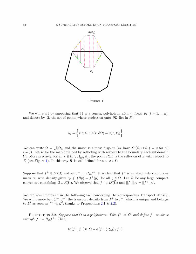
52 3. SUMMABILITY ESTIMATES ON TRANSPORT DENSITIES
Ωi
R(Ωi)
Fi
Figure 1
We will start by supposing that Ω is a convex polyhedron with n faces Fi (i = 1, ..., n),and denote by Ωi the set of points whose projection onto ∂Ω lies in Fi:
Ωi =
x ∈ Ω : d(x, ∂Ω) = d(x, Fi)
.
We can write Ω =⋃i Ωi, and the union is almost disjoint (we have Ld(Ωi ∩ Ωj) = 0 for all
i 6= j). Let R be the map obtained by reflecting with respect to the boundary each subdomainΩi. More precisely, for all x ∈ Ωi \
⋃j 6=i Ωj , the point R(x) is the reflexion of x with respect to
Fi (see Figure 1). In this way R is well-defined for a.e. x ∈ Ω.
Suppose that f+ ∈ Lp(Ω) and set f− := R#f+. It is clear that f− is an absolutely continuous
measure, with density given by f−(Ry) = f+(y) for all y ∈ Ω. Let Ω be any large compact
convex set containing Ω ∪R(Ω). We observe that f− ∈ Lp(Ω) and ||f−||Lp = ||f+||Lp .
We are now interested in the following fact concerning the corresponding transport density.We will denote by σ(f+, f−) the transport density from f+ to f− (which is unique and belongsto L1 as soon as f+ Ld; thanks to Propositions 2.1 & 2.2).
Proposition 3.2. Suppose that Ω is a polyhedron. Take f+ Ld and define f− as abovethrough f− = R#f
+. Then,
(σ(f+, f−)) Ω = σ(f+, (P∂Ω)#f+).
3.2. Lp ESTIMATES VIA SYMMETRIZATION 53
Moreover, if f+ ∈ Lp(Ω), then the transport density between f+ and (P∂Ω)#f+ is in Lp(Ω).
Proof. First, we will show that R is an optimal transport map from f+ to f−. Set,
u(x) =
d(x, ∂Ω) if x ∈ Ω,
−d(x, ∂Ω) else.
From |x−R(x)| = 2|x− P∂Ω(x)|, we have
∫Ω|x−R(x)|df+(x) = 2
∫Ω|x− P∂Ω(x)| df+(x).
On the other hand, u is 1-Lip and
∫Ωud(f+ − f−) =
∫Ω|x− P∂Ω(x)| f+(x) dx+
∫Ω|R(x)− P∂Ω(R(x))| f+(x) dx
= 2
∫Ω|x− P∂Ω(x)| df+(x).
Consequently, R is an optimal transport map between f+ and f−, and u is a Kantorovichpotential. We observe that the segment [x,R(x)] intersects ∂Ω at the point P∂Ω(x) and thatwe have
[x,R(x)] ∩ Ω = [x, P∂Ω(x)].
But the map x 7→ P∂Ω(x) is of course optimal in the transport from f+ to (P∂Ω)#f+. Hence,
using (2.2), we immediately get
(σ(f+, f−)) Ω = σ(f+, (P∂Ω)#f+)
and we conclude by using Proposition 2.4.
Now, we will give a more general construction, inspired from the previous one, which will allowto deal with the case of a domain with an exterior ball condition.
Suppose that the boundary of Ω is a union of a finite number of parts of sphere of radius
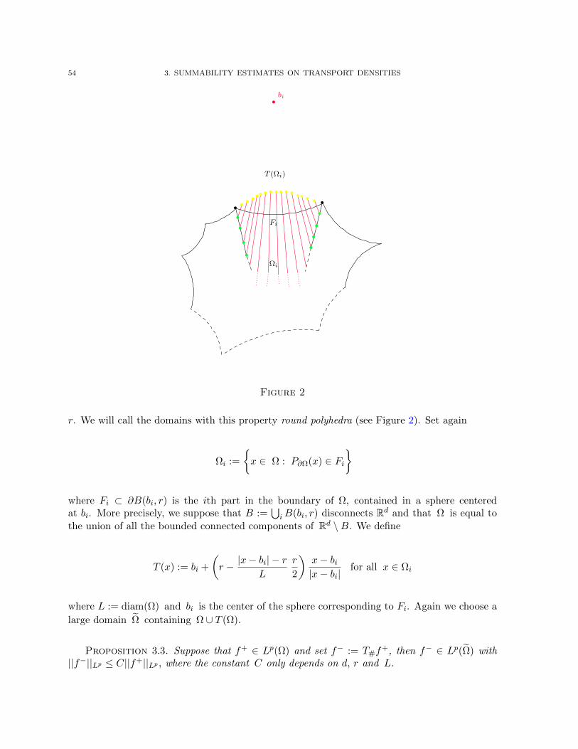
54 3. SUMMABILITY ESTIMATES ON TRANSPORT DENSITIES
bi
T (Ωi)
Ωi
Fi
Figure 2
r. We will call the domains with this property round polyhedra (see Figure 2). Set again
Ωi :=
x ∈ Ω : P∂Ω(x) ∈ Fi
where Fi ⊂ ∂B(bi, r) is the ith part in the boundary of Ω, contained in a sphere centeredat bi. More precisely, we suppose that B :=
⋃iB(bi, r) disconnects Rd and that Ω is equal to
the union of all the bounded connected components of Rd \B. We define
T (x) := bi +
(r − |x− bi| − r
L
r
2
)x− bi|x− bi|
for all x ∈ Ωi
where L := diam(Ω) and bi is the center of the sphere corresponding to Fi. Again we choose a
large domain Ω containing Ω ∪ T (Ω).
Proposition 3.3. Suppose that f+ ∈ Lp(Ω) and set f− := T#f+, then f− ∈ Lp(Ω) with
||f−||Lp ≤ C||f+||Lp , where the constant C only depends on d, r and L.
3.2. Lp ESTIMATES VIA SYMMETRIZATION 55
Proof. Compute the Jacobian of the map T : on Ωi, we have
DT (x) =r
2L
(−I +
r + 2L
|x− bi|(I − e(x)⊗ e(x)
)),
where e(x) := (x − bi)/|x − bi|. It is easy to see that DT (x) is a symmetric matrix withone eigenvalue equals to − r
2L and d− 1 eigenvalues equal to
λ(x) :=r
2L
r + 2L− |x− bi||x− bi|
=r
2L
(r + 2L
|x− bi|− 1
).
Using |x− bi| ≤ r + L, we get
λ(x) ≥ r
2(r + L).
This provides, for J := |det(DT )|, the lower bound
J(x) ≥ rd
2d(r + L)d−1L
which is, by the way, independent of i and of the number of spherical parts composing ∂Ω.Moreover, from f−(T (x)) = f+(x)/J(x), we get
∫|f−(y)|p dy =
∫|f−(y)|p−1 df− =
∫|f−(T (x))|p−1 df+ =
∫f+(x)p
J(x)p−1dx ≤ C
∫f+(x)p dx,
where C := (inf J(x))1−p > 0. By raising to power 1/p, this provides
||f−||Lp ≤ C(r, L, d)1/p−1||f+||Lp
and the constant can be taken independent of p. In particular, the estimate is also valid forp =∞.
Proposition 3.4. Suppose that Ω is a round polyhedron. Take f+ Ld and define f− asabove through f− = T#f
+. Then
(σ(f+, f−)) Ω = σ(f+, (P∂Ω)#f+).
56 3. SUMMABILITY ESTIMATES ON TRANSPORT DENSITIES
Moreover, if f+ ∈ Lp(Ω), then the transport density between f+ and (P∂Ω)#f+ is in Lp(Ω).
Proof. The proof will follow the same lines of Proposition 3.2. We will show again theoptimality of T for the transport of f+ to f− by producing a Kantorovich potential. In thiscase, we set
u(x) = mini=1,..,n
|x− bi|.
The function u is of course 1-Lip and we have
∫Ωud(f+ − f−) =
∫Ωu(x)f+(x) dx−
∫Ωu(T (x))f+(x) dx
=
n∑i=1
∫Ωi
u(x)f+(x) dx−∫
Ωi
u(T (x))f+(x) dx
=
n∑i=1
∫Ωi
(|x− bi| − |T (x)− bi|) f+(x) dx.
Yet, by definition of T , the points bi, x and T (x) are aligned (with T (x) ∈ [x, bi]) and then,|x− bi| − |T (x)− bi| = |x− T (x)|. So, we get∫
Ωud(f+ − f−) =
∫Ω|x− T (x)|f+(x) dx.
Consequently, T is an optimal transport map between f+ and f−, and u is the correspond-ing Kantorovich potential. Now, we observe in this case as well that the segment [x, T (x)]intersects ∂Ω at the point P∂Ω(x) and that we have
[x, T (x)] ∩ Ω = [x, P∂Ω(x)].
Hence, using (2.2) again, we immediately get
(σ(f+, f−)) Ω = σ(f+, (P∂Ω)#f+)
and we conclude by Proposition 2.4.
Remark 3.5. One can easily see that, both in Propositions 3.2 and 3.4, the restriction prop-erty of the transport density σ also holds for the optimal flow w of (3.1).
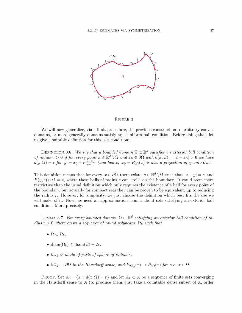
3.2. Lp ESTIMATES VIA SYMMETRIZATION 57
Ω
∂Ωk
Figure 3
We will now generalize, via a limit procedure, the previous construction to arbitrary convexdomains, or more generally domains satisfying a uniform ball condition. Before doing that, letus give a suitable definition for this last condition:
Definition 3.6. We say that a bounded domain Ω ⊂ Rd satisfies an exterior ball conditionof radius r > 0 if for every point x ∈ Rd \ Ω and x0 ∈ ∂Ω with d(x,Ω) = |x − x0| > 0 we haved(y,Ω) = r for y := x0 + r x−x0
|x−x0| (and hence, x0 = P∂Ω(x) is also a projection of y onto ∂Ω).
This definition means that for every x ∈ ∂Ω there exists y ∈ Rd \Ω such that |x− y| = r andB(y, r) ∩ Ω = ∅, where these balls of radius r can “roll” on the boundary. It could seem morerestrictive than the usual definition which only requires the existence of a ball for every point ofthe boundary, but actually for compact sets they can be proven to be equivalent, up to reducingthe radius r. However, for simplicity, we just choose the definition which best fits the use wewill make of it. Now, we need an approximation lemma about sets satisfying an exterior ballcondition. More precisely:
Lemma 3.7. For every bounded domain Ω ⊂ Rd satisfying an exterior ball condition of ra-dius r > 0, there exists a sequence of round polyhedra Ωk such that
• Ω ⊂ Ωk,
• diam(Ωk) ≤ diam(Ω) + 2r,
• ∂Ωk is made of parts of sphere of radius r,
• ∂Ωk → ∂Ω in the Hausdorff sense, and P∂Ωk(x)→ P∂Ω(x) for a.e. x ∈ Ω.
Proof. Set A := x : d(x,Ω) = r and let Ak ⊂ A be a sequence of finite sets convergingin the Hausdorff sense to A (to produce them, just take a countable dense subset of A, order
58 3. SUMMABILITY ESTIMATES ON TRANSPORT DENSITIES
its points, and put the first k points in Ak). Set Ωk := x : d(x,Ω) ≤ r ≤ d(x,Ak). For largek, the set Ωk is a round polyhedron with boundary composed of parts of spheres of radius rcentered at points of Ak. Indeed, it is clear that the points on ∂Ωk are contained either in thesespheres, or in A, but as soon as the Hausdorff distance between Ak and A is smaller than r,we have d(x,Ak) < r for every x ∈ A, hence A ∩ Ωk = ∅ and the points of A cannot be on theboundary of Ωk. Moreover, one easily see that we have Ω ⊂ Ωk and that Ωk is contained in acompact set. Up to a subsequence, we can suppose Ωk → Ω′ in the Hausdorff sense, with Ω ⊂ Ω′.Yet, passing to the limit in the definition of Ωk, we get Ω′ ⊂ x : d(x,Ω) ≤ r ≤ d(x,A). Thisis enough to obtain Ω′ = Ω : take a point x with d(x,Ω) ≤ r ≤ d(x,A) and suppose that itdoes not belong to Ω; let x0 ∈ ∂Ω be such that |x − x0| = d(x,Ω) and set y := x0 + r x−x0
|x−x0| .
From the definition 3.6, we have that y ∈ A, which is a contradiction, as d(x, y) < r.
Hence, we have Ω ⊂ Ωk and Ωk → Ω in the Hausdorff sense. The last part of the state-ment (convergence of the boundaries and of the projections onto the boundaries) is a generalconsequence of these facts.
We can now state the following
Proposition 3.8. Suppose that Ω ⊂ Rd is a compact domain satisfying a uniform exterior
ball condition of radius r > 0. Then there exists a larger domain Ω such that for every positive
measure f+ Ld, there exists f− Ld, supported on Ω \ Ω with
(σ(f+, f−)) Ω = σ(f+, (P∂Ω)#f+).
Moreover, for every p ∈ [1,+∞], we have
||f−||Lp(Ω)
≤ C||f+||Lp(Ω),
where C is a constant only depending on d, r and L := diam(Ω).
Proof. It is enough to act by approximation. In the case where Ω is convex, we can writeit as an intersection of half-spaces, and hence we can approximate Ω as the limit of a sequenceof polyhedra Ωk, while in the case where Ω satisfies a uniform exterior ball condition, we willwrite it as a limit of round polyhedra (see Figure 3) as we pointed out in Lemma 3.7. Then, wejust build the reflection maps Rk (or Tk) as in Propositions 3.2 and 3.4, and we get a sequence
of measures f−k supported on Ω \ Ωk with ||f−k ||Lp(Ω)≤ C||f+||Lp(Ωk) = C||f+||Lp(Ω). We also
have
(σ(f+, f−k )) Ω = σ(f+, (P∂Ωk)#f+) Ω.
Then, it is enough to extract a converging subsequence from the sequence f−k , note that we have(P∂Ωk)#f
+ (P∂Ω)#f+, and use Proposition 1.3.
As a consequence, we can now obtain
3.3. AN L∞ BOUND ON f− WITH RESPECT TO THE SURFACE MEASURE ON ∂Ω IS NOT ENOUGH 59
Theorem 3.9. Suppose that Ω satisfies a uniform exterior ball condition of radius r > 0.Then, the transport density σ between f+ and (P∂Ω)#f
+ is in Lp(Ω) provided f+ is in Lp(Ω),and
||σ||Lp(Ω) ≤ C||f+||Lp(Ω),
where the constant C only depends on d, r and L = diam(Ω).
Proof. We just need to use Proposition 3.8, which guarantees that σ is the restriction toΩ of the transport density between two Lp measures.
We finish this section by two remarks on the proof of the above result.
Remark 3.10. In this particular case where the transport has not a fixed target measure on∂Ω, the transport density σ linearly depends on f+: in this case, Lp estimates could be obtainedvia interpolation (via the celebrated Marcinkiewicz interpolation theorem, [86, 114]) as soon asone has L1 and L∞ estimates. Since L1 (and Lp for p < d′) are well-known, this means thatit would be enough to write L∞ estimates. Yet, we did not see any significant simplification inconcentrating on L∞ estimates instead of Lp, which is the reason why we decided not to evokegeneral interpolation theorems but we performed explicit estimates.
Remark 3.11. Another observation concerns the fact that we proved Proposition 3.8 by ap-proximation. Apart from the fact that we first developed the convex case (just for the sake ofsimplicity), the reader would have preferred a direct formulation, valid in the case of an arbi-trary domain Ω with an exterior ball condition, instead of passing through round polyhedra. Thiswould be possible, by defining a map T (x) := P∂Ω(x) + c(P∂Ω(x)−x), for small c > 0. It can beproven, by studying the properties of the Jacobian of P∂Ω, that T is injective and |det(DT )| isbounded from below as soon as c is small (depending on r and L), but we considered that theproof in the case of round polyhedra was easier.
3.3. An L∞ bound on f− with respect to the surface measure on ∂Ω is not enough
In this section, we show that the L∞ estimates for the transport density (again, note byRemark 3.10 that the case p =∞ is the most interesting one) fail if we only assume summabil-ity (or boundedness) of the densities of f+ w.r.t. the Lebesgue measure on Ω and of f− w.r.t.the Hausdorff measure Hd−1 on ∂Ω. Indeed, when we consider a domain Ω with a uniformexterior ball condition and we take f+ ∈ L∞, we can easily prove that (P∂Ω)#f
+ has a bounded
density w.r.t. Hd−1 ∂Ω. One could wonder whether this is the correct assumption to prove,for instance, σ ∈ L∞, and the answer is negative.
We will construct an example of f±, where f+ has a bounded density w.r.t. Ld in Ω and f−
w.r.t. Hd−1 ∂Ω (for instance Ω is a big square containing the support of f+ and its bound-ary contains the support of f−), but σ /∈ L∞ (we will also investigate the summability of σ). Set
f+ := L2 A, f− := H1 ([2, 3]× 0)

60 3. SUMMABILITY ESTIMATES ON TRANSPORT DENSITIES
x
T (x)
f+
f−
B2r
Figure 4
where A is a trapeze with vertices (0, 0), (1, 0), (1, 45) and (0, 6
5) (see Figure 4). For everyε ∈ [0, 1], let lε be the segment joining the two points (0, w(ε)) and (2 + ε, 0), where
w(ε) :=2(2 + ε)ε
3 + 2ε.
First, it is easy to see that f+(∆ε) = f−(∆ε), for every ε ∈ [0, 1], where ∆ε is the trianglelimited by (0, 0), (2 + ε, 0) and (0, w(ε)). Then by [95] (or exactly as in Chapter 5), we canconstruct an optimal mapping T , which pushes f+ to f−, with lε as its transport rays.
Let σ be the transport density between f+ and f−. For simplicity of notation, we denote theball of center (2, 0) and radius r by Br, and in this case we have
σ(B2r) =
∫H1(B2r ∩ [x, y]) dγ(x, y) ≥ r γ ((x, y) : Br ∩ [x, y] 6= ∅) ,
where we used the fact that for every (x, y) s.t. Br ∩ [x, y] 6= ∅, we have H1(B2r ∩ [x, y]) ≥ r.Note that there exists a value εr ∈ (0, 1) such that x : Br ∩ [x, T (x)] 6= ∅ = ∆εr and lεr istangent to the ball Br. Hence,
σ(B2r) ≥ rf+(x : Br ∩ [x, T (x)] 6= ∅) = rf+(∆εr) ' rεr.
If we denote by θ the angle between the two segments [(0, 0), (2 + εr, 0)] and lεr , then we

3.3. AN L∞ BOUND ON f− WITH RESPECT TO THE SURFACE MEASURE ON ∂Ω IS NOT ENOUGH 61
have
sin(θ) =r
εr.
Yet, sin(θ) ' εr for r small enough. So, we get εr ' r12 . Thus, for r small enough
(3.3) σ(B2r) ≥ cr32 ,
which implies that σ cannot be bounded in a neighborhood of (2, 0), otherwise we would have
Cr2 = ||σ||L∞(∆1)|B2r| ≥ σ(B2r) ≥ cr32
which is a contradiction for small r. In addition, it is possible to see σ /∈ L4(∆1), otherwise, byHolder inequality, we would get
σ(B2r)
r3/2≤|B2r|3/4
(∫B2r
σ4)1/4
r3/2→ 0,
which is a contradiction with (3.3).
Actually, a finer analysis even proves σ ∈ Lp(∆1) if and only if p < 3. To prove this we needto use heavier computations. Fix ε0 small enough and take x ∈ ∆ε0 : there exist ε ∈ [0, ε0] ands ∈ [0, 1] such that
x = (1− s)(2 + ε, 0) + s(0, w(ε)).
Recalling (2.1), for all ϕ ∈ C(∆ε0), we have
< σ,ϕ >:=
∫ 1
0
∫∆ε0
|x− T (x) |ϕ((1− t)x+ tT (x)) f+(x) dx dt.
So, by a change of variable, we get, in the variable (ε, s),
σ(ε, s) =
√(2 + ε)2 + w(ε)2
∫ 1s f
+((1− t)(2 + ε), tw(ε))|J(ε, t)|dt|J(ε, s)|
=
√(2 + ε)2 + w(ε)2
∫ 11− 1
2+ε|J(ε, t)|dt
|J(ε, s)|'
∫ 11− 1
2+ε|J(ε, t)|dt
|J(ε, s)|,

62 3. SUMMABILITY ESTIMATES ON TRANSPORT DENSITIES
where |J | := |D(ε,s)(x1, x2)|. Using the fact that |J(ε, s)| ' s+ ε, we get
σ(ε, s) ' 1
s+ εand
||σ||pLp(∆1) '∫ ε0
0
∫ 1
0
1
(s+ ε)p−1ds dε '
∫ ε0
0
1
εp−2dε.
Notice that as d = 2 and f+ ∈ L∞(∆1), by Proposition 2.3 we know that automaticallyσ ∈ Lp(∆1) for all p < 2. The fact that here we get σ ∈ Lp(∆1) for all p < 3 depends onthe fact that we send a mass f+ to a mass f− which is distributed on a segment, and not to aDirac mass. We are not in the worst possible case !
So, we have shown that if f+ is a bounded density w.r.t. Ld and f− is a bounded densityw.r.t. Hd−1 ∂Ω (and, f− is different than the projection of f+ onto ∂Ω), then the transportdensity σ between f+ and f− is not, in general, in Lp, for all p ≥ 3. In Chapter 6, we will studythe summability of the transport density σ between two measures, f+ and f−, concentratedon the boundary.

CHAPTER 4
Summability estimates with boundary costs
In this chapter we analyze a mass transportation problem in a compact domain with the possibility
to transport mass to/from the boundary, paying a cost given by the Euclidean distance plus an extra cost
depending on the exit/entrance point. This problem appears in import/export model, as well as in some
shape optimization problems. We study the Lp summability of the transport density σ which does not
follow from Proposition 2.4, as the target measures are not absolutely continuous but they have some
parts which are concentrated on the boundary. We also provide the relevant duality arguments to connect
the corresponding Beckmann and Kantorovich problems to a formulation with Kantorovich potentials with
Dirichlet boundary conditions.
This chapter is taken from my article [54], which will be published in Journal ofConvex Analysis.
In [90], the authors introduce a variant of the classical Kantorovich problem (KP). They studya mass transportation problem between two masses f+ and f− (which do not have a priori thesame total mass) with the possibility of transporting some mass to/from the boundary, payingthe transport cost c(x, y) = |x−y| plus an extra cost g−(y) for each unit of mass that comes outfrom a point y ∈ ∂Ω (the export taxes) or −g+(x) for each unit of mass that enters at the pointx ∈ ∂Ω (the import taxes). This means that we can use ∂Ω as an infinite reserve/repository, wecan take as much mass as we wish from the boundary, or send back as much mass as we want,provided that we pay the transportation cost plus the import/export taxes. In other words,given the set
Πb(f+, f−) :=γ ∈M+(Ω× Ω) : ((Πx)#γ)
Ω = f+, ((Πy)#γ)
Ω = f−
,
we minimize the quantity
(KPb) min
∫Ω×Ω|x− y|dγ +
∫∂Ωg− d(Πy)#γ −
∫∂Ωg+ d(Πx)#γ : γ ∈ Πb(f+, f−)
.
The equality min (KP) = min (BP) (see Section 2.3) implies that min (KPb) = min (BPb),where (BPb) is the following variant of (BP)
63
64 4. SUMMABILITY ESTIMATES ON TRANSPORT DENSITIES
min
|w|(Ω) +
∫∂Ωg− dχ− −
∫∂Ωg+ dχ+ : w ∈Md(Ω), χ ∈M(∂Ω), ∇ · w = f + χ
.
On the other hand, the authors of [90] prove that the dual of (KPb) (or equivalently, (BPb)) isthe following
(DPb) sup
∫Ωud(f+ − f−) : u ∈ Lip1(Ω), g+ ≤ u ≤ g− on ∂Ω
.
We will give an alternative proof for this duality formula that we consider simpler than that in[90]. In fact, one can easily see that it follows immediately from a formal inf-sup exchange: wemay look at the problem (KPb), we get
min
sup
∫Ωud(f + χ) : u ∈ Lip1(Ω)
+
∫∂Ωg− χ− −
∫∂Ωg+ dχ+ : χ± ∈M+(∂Ω)
and consider interchanging inf and sup:
= sup
∫Ωudf + inf
∫∂Ω
(u− g+) dχ+ +
∫∂Ω
(g− − u) dχ− : χ± ∈M+(∂Ω)
: u ∈ Lip1(Ω)
.
Yet,
inf
∫∂Ω
(u− g+)dχ+ +
∫∂Ω
(g− − u)dχ− : χ± ∈M+(∂Ω)
=
0 if g+ ≤ u ≤ g− on ∂Ω
−∞ else.
4.1. Monge-Kantorovich problems with boundary costs: existence,characterization and duality
In this section, we analyze the problem (KPb). Except for the duality proof, we will alsodecompose it into subproblems. One of this subproblems involves a transport plan γib (withits transport density σib), where i and b stand for interior and boundary (conversely, we alsohave a transport plan γbi with σbi). We will show that some questions, including summabilityof the transport density σ, reduce to the study of the summability of σib and σbi. First of all,we suppose g± ∈ C(∂Ω) and we assume the following inequality
(4.1) g+(x)− g−(y) ≤ |x− y| for all x, y ∈ ∂Ω.
Under this assumption, we have the following:

4.1. MONGE-KANTOROVICH PROBLEMS WITH BOUNDARY COSTS 65
Proposition 4.1. (KPb) reaches a minimum.
Proof. Set
K(γ) :=
∫Ω×Ω|x− y|dγ +
∫∂Ωg− d(Πy)#γ −
∫∂Ωg+ d(Πx)#γ, ∀ γ ∈M+(Ω× Ω).
Then, K is continuous with respect to the weak convergence of measures in Πb(f+, f−). Indeed,if (γn)n is a sequence in Πb(f+, f−) such that γnγ, then, for every n, there exists χ±n ∈M+(∂Ω) such that
(Πx)#γn = f+ + χ+n , (Πy)#γn = f− + χ−n
and
χ±n χ±,
where (Πx)#γ = f+ + χ+ and (Πy)#γ = f− + χ−. As g± ∈ C(∂Ω), then
K(γn)→ K(γ).
On the other hand, we observe that if γ ∈ Πb(f+, f−) and γ := γ (∂Ω× ∂Ω)c, then γ alsobelongs to Πb(f+, f−). In addition, we have∫
Ω×Ω|x− y|dγ +
∫∂Ωg− d(Πy)#γ −
∫∂Ωg+ d(Πx)#γ
=
∫∂Ω×∂Ω
(|x−y|+g−(y)−g+(x)) dγ +
∫(∂Ω×∂Ω)c
|x−y| dγ +
∫Ω×∂Ω
g−(y) dγ −∫∂Ω×Ω
g+(x) dγ.
As
|x− y|+ g−(y)− g+(x) ≥ 0,
we get
∫Ω×Ω|x− y|dγ +
∫∂Ωg− d(Πy)#γ −
∫∂Ωg+ d(Πx)#γ
≥∫
Ω×Ω|x− y|dγ +
∫∂Ωg− d(Πy)#γ −
∫∂Ωg+ d(Πx)#γ.
Now, let (γn)n ⊂ Πb(f+, f−) be a minimizing sequence. Then, we can suppose that
γn(∂Ω× ∂Ω) = 0.

66 4. SUMMABILITY ESTIMATES ON TRANSPORT DENSITIES
In this case, we get
γn(Ω× Ω) ≤ γn(Ω0 × Ω) + γn(Ω× Ω0)
= f+(Ω) + f−(Ω).
Hence, there exist a subsequence (γnk)nk and a plan γ ∈ Πb(f+, f−) such that γnkγ. But,the continuity of K implies that this plan γ is in fact a minimizer for (KPb).
Let us note that the proof of the duality formula of (KPb), in [90], is based on the Fenchel-Rocafellar duality Theorem and it is decomposed into two steps: firstly, the authors supposethat the inequality in (4.1) is strict and secondly, they use an approximation argument to coverthe other case. Now, we want to give an alternative proof for this duality formula, similar tothe one introduced in Proposition 1.2, but, here, via a perturbation of the boundary costs g±.
Proposition 4.2. Under the assumption (4.1), we have the following equality
min
∫Ω×Ω|x− y| dγ +
∫∂Ωg− d(Πy)#γ −
∫∂Ωg+ d(Πx)#γ : γ ∈ Πb(f+, f−)
(KPb)
= sup
∫Ωu d(f+ − f−) : u ∈ Lip1(Ω), g+ ≤ u ≤ g− on ∂Ω
(DPb).
Notice that if (4.1) is not satisfied, then both sides of this equality are −∞.
Proof. For every (p+, p−) ∈ C(∂Ω)× C(∂Ω), set
H(p+, p−) := − sup
∫Ωud(f+ − f−) : u ∈ Lip1(Ω), g+ + p+ ≤ u ≤ g− − p− on ∂Ω
.
First, it is easy to see that H(p+, p−) ∈ R ∪ +∞. In addition, we claim that H is con-vex and l.s.c.
• For convexity: take t ∈ (0, 1) and (p+0 , p
−0 ), (p+
1 , p−1 ) ∈ C(∂Ω) × C(∂Ω), and let u0, u1 be
their optimal potentials. Set
p+t := (1− t)p+
0 + tp+1 , p
−t := (1− t)p−0 + tp−1
and
ut := (1− t)u0 + tu1.
4.1. MONGE-KANTOROVICH PROBLEMS WITH BOUNDARY COSTS 67
As
g+ + p+0 ≤ u0 ≤ g− − p−0 and g+ + p+
1 ≤ u1 ≤ g− − p−1 on ∂Ω,
then
g+ + p+t ≤ ut ≤ g− − p
−t on ∂Ω.
In addition, ut is 1-Lipschitz. Consequently, ut is admissible in the max defining −H(p+t , p
−t )
and then,
H(p+t , p
−t ) ≤ −
∫Ωut d(f+ − f−) = (1− t)H(p+
0 , p−0 ) + tH(p+
1 , p−1 ).
• For semi-continuity: take p+n → p+ and p−n → p− uniformly on ∂Ω. Let (p+
nk, p−nk)nk
be a subsequence realizing the lim inf of H(p+n , p
−n ) (for simplicity of notation, we still denote
it (p+n , p
−n )n) and let (un)n be their corresponding optimal potentials. As un is a 1-Lipschitz
function and (p+n )n, (p−n )n are equibounded, then, by Ascoli-Arzela Theorem, there exist a 1-
Lipschitz function u and a subsequence (unk)nk such that unk → u uniformly in Ω. As
g+ + p+nk≤ unk ≤ g
− − p−nk on ∂Ω,
then
g+ + p+ ≤ u ≤ g− − p− on ∂Ω.
Consequently, the potential u is admissible in the max defining −H(p+, p−) and, one has
H(p+, p−) ≤ −∫
Ωu d(f+ − f−) = lim inf
nH(p+
n , p−n ).
Hence, we get H?? = H. In particular, H??(0, 0) = H(0, 0). But by the definition of H,we have H(0, 0) = − sup (DPb). On the other hand, let us compute H??(0, 0). Take χ± inM(∂Ω), then we have
H?(χ+, χ−) := supp± ∈C(∂Ω)
∫∂Ωp+ dχ+ +
∫∂Ωp− dχ− −H(p+, p−)
= supp±∈C(∂Ω), u∈Lip1(Ω)
∫∂Ωp+ dχ++
∫∂Ωp− dχ−+
∫Ωud(f+−f−) : g++p+ ≤ u ≤ g−−p− on ∂Ω
.
If χ+ /∈ M+(∂Ω), i.e. there exists p+0 ∈ C(∂Ω) such that p+
0 ≥ 0 and∫∂Ω p
+0 dχ+ < 0, we
may see that
H?(χ+, χ−) ≥ −n∫∂Ωp+
0 dχ+ +
∫∂Ωg− dχ− −
∫∂Ωg+ dχ+ −→
n→+∞+∞
68 4. SUMMABILITY ESTIMATES ON TRANSPORT DENSITIES
and similarly, if χ− /∈ M+(∂Ω). Now, suppose both χ± ∈ M+(∂Ω). As g+ + p+ ≤ u ≤g− − p− on ∂Ω, we should choose the largest possible p+ and p−, i.e. p+ = u − g+ andp− = g− − u on ∂Ω. Hence, we get
H?(χ+, χ−) = sup
∫Ωu d(f + χ) : u ∈ Lip1(Ω)
+
∫∂Ωg− dχ− −
∫∂Ωg+ dχ+.
By Proposition 1.2, we infer that
H?(χ+, χ−) = min
∫Ω×Ω|x− y|dγ : γ ∈ Π(f+ + χ+, f− + χ−)
+
∫∂Ωg− dχ− −
∫∂Ωg+ dχ+
= min
∫Ω×Ω|x− y|dγ +
∫∂Ωg− d(Πy)#γ −
∫∂Ωg+ d(Πx)#γ : γ ∈ Π(f+ + χ+, f− + χ−)
.
Finally, we have
H??(0, 0) = sup
−H?(χ+, χ−) : χ+, χ− ∈M+(∂Ω)
= −min (KPb).
Let γ be a minimizer for (KPb) and let us denote by χ+ and χ− the two non-negative measuresconcentrated on the boundary of Ω such that (Πx)#γ = f+ + χ+ and (Πy)#γ = f− + χ−.Then, we may see easily that γ is also a minimizer for the following problem
min
∫Ω×Ω|x− y| dγ : γ ∈ Π(µ+, µ−)
where µ± := f± + χ±. Moreover, if u is a maximizer for (DPb), then we have the follow-ing:
Proposition 4.3. The function u is also a Kantorovich potential between µ+ and µ−, i.e.,u solves the following problem
sup
∫Ωϕd(µ+ − µ−) : ϕ ∈ Lip1(Ω)
.

4.1. MONGE-KANTOROVICH PROBLEMS WITH BOUNDARY COSTS 69
Proof. Let ϕ be a Kantorovich potential between µ+ and µ−. As u is 1-Lip and g+ ≤u ≤ g− on ∂Ω, then we have
∫Ωud(f+ − f−) +
∫∂Ωg+ dχ+ −
∫∂Ωg− dχ− ≤
∫Ωud(µ+ − µ−) ≤
∫Ωϕd(µ+ − µ−).
Yet, by Proposition 1.2, we have
∫Ωϕd(µ+ − µ−) =
∫Ω×Ω|x− y|dγ,
where γ is the fixed optimal transport plan for (KPb). Using Proposition 4.2, we infer thatthe above inequalities are in fact equalities and u is a Kantorovich potential between µ+ andµ−.
Now, suppose that Ω is convex and, set w := −σ∇u, where σ is the transport density associatedwith the optimal transport plan γ. Then, using Proposition 4.3, we infer that the vector measurew solves
min
|w|(Ω) : w ∈Md(Ω), ∇ · w = µ+ − µ−
.
Yet, from the fact that min (BPb) = min (KPb), we can conclude that the vector measurew and the boundary measure χ solve together (BPb) (χ± are the import/export measures). Inaddition, the pair (σ, u) solves the following system, which is a variant of the Monge-Kantorovichone:
(4.2)
−∇ · (σ∇u) = f+ − f− in Ω,
g+ ≤ u ≤ g− on ∂Ω,
|∇u| ≤ 1 in Ω,
|∇u| = 1 σ − a.e.
However, the same result will be true, even if Ω is not convex, by using the following:
Proposition 4.4. Suppose that
|g+(x)− g−(y)| ≤ |x− y| for all x, y ∈ ∂Ω,
i.e. g+ = g− := g where g is a 1-Lipschitz function on ∂Ω. Then there exists a minimizer γ?
for (KPb) such that for all (x, y) ∈ spt(γ?), we have [x, y] ⊂ Ω. In addition, if g is λ-Lipschitzwith λ < 1, then for any minimizer γ of (KPb) and for all (x, y) ∈ spt(γ), [x, y] ⊂ Ω.

70 4. SUMMABILITY ESTIMATES ON TRANSPORT DENSITIES
Proof. First of all, set
E :=
(x, y) ∈ Ω× Ω, [x, y] ⊂ Ω
.
Let us define the map p+ as follows
p+ : Ω× Ω 7→ ∂Ω× Ω
(x, y) 7→ (x′, y)
where x′ is the last point of intersection between the segment [x, y] and the boundary if(x, y) /∈ E and x′ = x else.
Also set
p− : Ω× Ω 7→ Ω× ∂Ω
(x, y) 7→ (x, y′)
where y′ is the first point of intersection between the segment [x, y] and the boundary if(x, y) /∈ E and y′ = y else.
Take a minimizer γ for (KPb) and, set
γ? := γ E + (p+)#(γ Ec) + (p−)#(γ Ec).
It is easy to see that γ? ∈ Πb(f+, f−). Moreover, γ? is better than γ in (KPb), i.e., K(γ?) ≤K(γ). Indeed, we have∫
Ω×Ω|x− y|dγ? +
∫∂Ωg d(Πy)#γ
? −∫∂Ωg d(Πx)#γ
?
=
∫E|x− y|dγ +
∫Ec
(|x− y′|+ |x′ − y|+ g(y′)− g(x′)) dγ +
∫∂Ωg d(Πy)#γ −
∫∂Ωg d(Πx)#γ.
Yet,
|x− y′|+ |x′ − y|+ g(y′)− g(x′) ≤ |x− y′|+ |x′ − y|+ |x′ − y′| = |x− y|.
Consequently, γ? is a minimizer for (KPb) and, for all (x, y) ∈ spt(γ?), we have [x, y] ⊂ Ω.The second statement follows directly from the last inequality, which becomes strict.

4.1. MONGE-KANTOROVICH PROBLEMS WITH BOUNDARY COSTS 71
Using Proposition 4.4, even if Ω is not convex, we infer that there is a solution (σ, u) to thefollowing system, provided that the boundary cost g is 1-Lip,
(4.3)
−∇ · (σ∇u) = f in Ω
u = g on ∂Ω,
|∇u| ≤ 1 in Ω,
|∇u| = 1 σ − a.e.
We note that this system describe the growth of a sandpile on a bounded table, with a wall onthe boundary of a height g, under the action of a vertical source here modeled by f (see [46]).
Now, we are interested to study the Lp summability of the transport density σ, which doesnot follow from Proposition 2.4, since in this case the source and target measures are not in Lp
as they have some parts, χ±, which are concentrated on ∂Ω. First of all, we note that to get aLp summability on σ, it is natural to suppose that g is strictly better than 1-Lipschitz. Indeed,we can find a positive density f ∈ Lp(Ω) and a boundary measure χ ∈ M+(∂Ω) such that thetransport density σ between f and χ is not in Lp(Ω) (see, for instance, Section 3.3). So, ifu is the Kantorovich potential between f and χ (which is 1-Lipschitz), then (σ, u) solves (4.3)with g = u.
For this aim, we want to decompose the optimal transport plan γ as a sum of three transportplans γii, γib and γbi, where each of these plans solves a particular transport problem (i and bstand for interior and boundary). Next, we will study the Lp summability of the transport den-sities σii, σib and σbi associated with these transport plans γii, γib and γbi, respectively. In thisway, we get the summability of the transport density σ associated with the optimal transportplan γ. Set,
γii := γ (Ω × Ω), γib := γ (Ω × ∂Ω), γbi := γ (∂Ω× Ω), γbb := γ (∂Ω× ∂Ω) = 0
and
ν+ := (Πx)#γib , ν− := (Πy)#γbi .
Consider the three following problems:
(P1) min
∫Ω×Ω|x− y|dγ : γ ∈ Π(f+ − ν+, f− − ν−)
(P2) min
∫Ω×Ω|x− y|dγ +
∫∂Ωg− dχ− : γ ∈ Π(ν+, χ−), spt(χ−) ⊂ ∂Ω
(P3) min
∫Ω×Ω|x− y|dγ −
∫∂Ωg+ dχ+ : γ ∈ Π(χ+, ν−), spt(χ+) ⊂ ∂Ω
.
72 4. SUMMABILITY ESTIMATES ON TRANSPORT DENSITIES
Let γ1 (resp. γ2 and γ3) be a solution of (P1) (resp. (P2) and (P3)). It is easy to see thatγii, γib and γbi are admissible in (P1), (P2) and (P3), respectively. Then, one has
∫Ω×Ω|x− y| dγ1 ≤
∫Ω×Ω|x− y| dγii,
∫Ω×Ω|x− y|dγ2 +
∫∂Ωg− d(Πy)#γ2 ≤
∫Ω×Ω|x− y|dγib +
∫∂Ωg− d(Πy)#γib
and ∫Ω×Ω|x− y|dγ3 −
∫∂Ωg+ d(Πx)#γ3 ≤
∫Ω×Ω|x− y| dγbi −
∫∂Ωg+ d(Πx)#γbi.
Yet, we see easily that the transport plan γ := γ1 + γ2 + γ3 belongs to Πb(f+, f−) and,we have
∫Ω×Ω|x− y|dγ +
∫∂Ωg− d(Πy)#γ −
∫∂Ωg+ d(Πx)#γ
≤∫
Ω×Ω|x− y|dγ +
∫∂Ωg− d(Πy)#γ −
∫∂Ωg+ d(Πx)#γ.
Then, γ also solves the problem (KPb) and so, we obtain that γii, γib and γbi solve (P1), (P2)and (P3), respectively.
We want to characterize the optimal transport plan γib. For this aim, let us define the multi-valued map Tib as follows
Tib(x) := argmin|x− y|+ g−(y), y ∈ ∂Ω
, for all x ∈ Ω.
We have the following
Lemma 4.5. The multi-valued map Tib has a Borel selector function.
Proof. To prove that Tib has a Borel selector function, it is enough to show that the graphof Tib is closed (see, for instance, [5, 40]). Take a sequence (xn, yn)n in the graph of Tib suchthat (xn, yn)→ (x, y). As yn ∈ Tib(xn), then we have
|xn − yn|+ g(yn) ≤ |xn − z|+ g(z), for all z ∈ ∂Ω.
4.2. Lp SUMMABILITY OF THE TRANSPORT DENSITY 73
Passing to the limit, we get
|x− y|+ g(y) ≤ |x− z|+ g(z), for all z ∈ ∂Ω
and then, y ∈ Tib(x).
Then, the plan γTib := (Id, Tib)#ν+ is admissible in (P2). In addition, for any admissible
γ 6= γTib in (P2), we have
∫Ω×∂Ω
(|x− y|+ g−(y)) dγTib <
∫Ω×∂Ω
(|x− y|+ g−(y)) dγ,
which implies that γib = γTib = (Id, Tib)#ν+. Moreover, the transport plan γib solves the
following problem
min
∫Ω×Ω|x− y|dγ : γ ∈ Π(ν+, (Tib)#ν
+)
.
In the same way, we get that the transport plan γbi is of the form (Tbi, Id)#ν−, where the
map Tbi is defined as follows
Tbi(y) := argmin|x− y| − g+(x), x ∈ ∂Ω
, for all y ∈ Ω.
In particular, γbi also solves
min
∫Ω×Ω|x− y|dγ : γ ∈ Π((Tbi)#ν
−, ν−)
.
Now, let σ (resp. σii, σib and σbi) be the transport density associated with the optimal trans-port plan γ (resp. γii, γib and γbi), therefore σ = σii + σib + σbi. By Proposition 2.4, thetransport density σii belongs to Lp(Ω) as soon as f± ∈ Lp(Ω). Hence, it is enough to studythe summability of σib (the case of σbi will be analogous), to get that of σ.
4.2. Lp summability of the transport density
In this section, we will study the Lp summability of the transport density σib, under the as-sumption that Ω satisfies a uniform exterior ball condition and, by supposing that the boundarycost g is λ-Lip with λ < 1 and semi-concave. First, we will suppose that Ω has a very particu-lar shape, i.e. its boundary is composed of parts of sphere of radius r (i.e., a round polyhedron),and then, by an approximation argument, we are able to generalize the result to any domainhaving a uniform exterior ball. Let us consider again the following transport problem

74 4. SUMMABILITY ESTIMATES ON TRANSPORT DENSITIES
(P) min
∫Ω×Ω|x− y|dγ +
∫∂Ωg dχ : γ ∈ Π(f, χ), spt(χ) ⊂ ∂Ω
.
Suppose that the boundary cost g is λ-Lip with λ < 1 and, set
T (x) := argmin |x− y|+ g(y), y ∈ ∂Ω for all x ∈ Ω.
Then, we have the following:
Proposition 4.6. T (x) is a singleton Lebesgue-almost everywhere.
Proof. Set
φ(x) := min|x− y|+ g(y), y ∈ ∂Ω for all x ∈ Ω.
It is clear that φ is 1-Lip, therefore it is differentiable Lebesgue-almost everywhere. Take x0 ∈ Ωand suppose that there exist y0 and y1 ∈ ∂Ω such that
φ(x0) = |x0 − y0|+ g(y0) = |x0 − y1|+ g(y1).
As
φ(x)− |x− y0| ≤ g(y0) for all x ∈ Ω,
then the function: x 7→ φ(x)− |x− y0| reaches a maximum at x0 and so, ∇φ(x0) = x0−y0
|x0−y0| . In
the same way, we get ∇φ(x0) = x0−y1
|x0−y1| . Hence, we have x0−y0
|x0−y0| = x0−y1
|x0−y1| , which is a contradic-
tion as y1 is in the half line with vertex x0 and passing through y0 (indeed in this case, one has|g(y0)− g(y1)| = |y0 − y1|).
Proposition 4.7. If x ∈ Ω and y ∈ T (x), then (x, y) ∩ ∂Ω = ∅.
Proof. Suppose that this is not the case, i.e. there exist x ∈ Ω, y ∈ T (x) and some pointz ∈ (x, y) ∩ ∂Ω. By definition of T , we have
|x− y|+ g(y) ≤ |x− z|+ g(z).
Then
|z − y| = |x− y| − |x− z| ≤ g(z)− g(y) ≤ λ|z − y|,
which is a contradiction.

4.2. Lp SUMMABILITY OF THE TRANSPORT DENSITY 75
Let Σ be the set of all the points x ∈ Ω where T (x) is not a singleton (thanks to Proposition4.6, one has Ld(Σ) = 0). Then, we have the following:
Proposition 4.8. If x ∈ Ω, y ∈ T (x) and z ∈ (x, y), then z /∈ Σ and T (z) = y.
Proof. For every w ∈ ∂Ω such that w /∈ T (x), we have
|z − y|+ g(y) = |x− y| − |x− z|+ g(y)
< |x− w|+ g(w)− |x− z|
≤ |z − w|+ g(w).
If w ∈ T (x), we also have
|z − y|+ g(y) = |x− w|+ g(w)− |x− z|
< |z − w|+ g(w),
where the last strict inequality follows from Proposition 4.7.
We recall that the plan γT := (Id, T )#f is the unique minimizer for (P). In addition, γT solvesthe following problem
min
∫Ω×Ω|x− y|dγ : γ ∈ Π(f, (T )#f)
.
For simplicity of notation, we will denote this minimizer by γ instead of γT . Let σ be thetransport density associated with the transport of f into (T )#f . By the definition of σ (see(2.1)), we have that, for all ϕ ∈ C(Ω),
< σ,ϕ > =
∫Ω×Ω
∫ 1
0|x− y|ϕ((1− t)x+ ty) dt dγ(x, y)
=
∫Ω
∫ 1
0|x− T (x)|ϕ((1− t)x+ tT (x))f(x) dtdx.
Then
σ =
∫ 1
0ft dt,
where
< ft, ϕ >:=
∫Ω|x− T (x)|ϕ(Tt(x))f(x) dx for all ϕ ∈ C(Ω)
76 4. SUMMABILITY ESTIMATES ON TRANSPORT DENSITIES
and
Tt(x) := (1− t)x+ tT (x) for all x ∈ Ω.
Notice that in the definition of ft, differently from what done in Section 2.2, we need to keep thefactor |x− T (x)|, which will be essential in the estimates. In addition, we have that ft Ld assoon as one has f Ld (see Proposition 2.2).
Now, we will introduce the two following propositions, whose proofs, for simplicity of expo-sition, are postponed to Section 4.4.
Proposition 4.9. Suppose that Ω is a round polyhedron and g is in C2(∂Ω) with |∇g| < 1.Then, the closure Σ of the set Σ is negligible and T is a C1 function on Ω\Σ.
We want to give an explicit formula of ft in terms of f and T . Let ϕ be in C(Ω), then wehave ∫
Ωϕ(y) dft(y) =
∫Ωϕ(Tt(x))|x− T (x)|f(x) dx.
Take a change of variable y = Tt(x). By Proposition 4.8, we get easily that
x =y − tT (y)
1− tand |x− T (x)| = |y − T (y)|
1− t.
Consequently, ∫Ωϕ(y)ft(y) dy =
∫Ωt
ϕ(y)|y − T (y)|
1− tf
(y − tT (y)
1− t
)|Jt(y)|dy,
where Ωt := Tt(Ω) and Jt(y) := (det(DTt(x)))−1 for all y = Tt(x) ∈ Ωt. Yet, this impliesthat
ft(y) =|y − T (y)|
1− tf
(y − tT (y)
1− t
)|Jt(y)|1Ωt(y) for a.e. y ∈ Ω.
Notice that a point y belongs to Ωt if and only if |y − T (y)| ≤ (1 − t)l(y) where l(y) isthe length of the transport ray containing y, i.e.,
l(y) := sup |x− T (x)| : x ∈ Ω ∩ T (y) + s(y − T (y)), s ≥ 1, T (x) = T (y) .
The following proposition gives a lower bound on the Jacobian Jt, which is in fact sufficient toprove our Lp estimates on the transport density σ:
4.2. Lp SUMMABILITY OF THE TRANSPORT DENSITY 77
Proposition 4.10. Suppose that Ω is a round polyhedron and g ∈ C2(∂Ω) with |∇g| ≤λ < 1. Then, there exists a constant C := C(d, diam(Ω), λ, r, M) > 0, where D2g ≤MI, suchthat, for a.e. x ∈ Ω, we have the following estimate
|det(DTt(x))| ≥ C(1− t).
We are now ready to prove the Lp summability of the transport density σ. Then, we have thefollowing result.
Proposition 4.11. Suppose that Ω is a round polyhedron and g ∈ C2(∂Ω) with |∇g| ≤λ < 1. Then, the transport density σ belongs to L∞(Ω) provided that f ∈ L∞(Ω).
Proof. By Proposition 4.10, we have
‖ σ ‖L∞(Ω) = supy ∈Ω
(∫ 1
0ft(y) dt
)
= supy ∈Ω
(∫ 1− |y−T (y)|l(y)
0
|y − T (y)|f(y−tT (y)1−t )
(1− t)|det(DTt(x))|dt
)
≤ C−1 ‖ f ‖L∞(Ω) supy ∈Ω
(∫ 1− |y−T (y)|l(y)
0
|y − T (y)|(1− t)2
dt
).
Yet, it is easy to see that
supy ∈Ω
∫ 1− |y−T (y)|l(y)
0
|y − T (y)|(1− t)2
dt ≤ diam(Ω).
Then,‖ σ ‖L∞(Ω) ≤ C ‖ f ‖L∞(Ω),
for some constant C depending only on d, diam(Ω), λ, r and M , where M is any constantsuch that D2g ≤MI.
Proposition 4.12. Let Ω be a round polyhedron, g ∈ C2(∂Ω) with |∇g| < 1 and supposef ∈ Lp(Ω) for some p ∈ [1,+∞]. Then, the transport density σ also belongs to Lp(Ω).
Proof. We observe that as the transport is between f and (T )#f , then the transportdensity σ linearly depends on f : in this case, Lp estimates could be obtained via interpolationas soon as one has L1 and L∞ estimates (see, for instance, [86]). In order to get an L1 estimate,it is enough to remember the implication f ∈ L1(Ω) ⇒ σ ∈ L1(Ω) from Proposition 2.2, andthat we have
||σ||L1(Ω) ≤ diam(Ω) ||f ||L1(Ω).
78 4. SUMMABILITY ESTIMATES ON TRANSPORT DENSITIES
In addition, the L∞ estimates follow from Proposition 4.11.
Remark 4.13. The same proof as in Proposition 4.11 could also be adapted to proving Propo-sition 4.12, but a suitable use of a Holder inequality would be required (see Proposition 9.2).
We will now generalize, via a limit procedure, the result of Proposition 4.12 to arbitrarydomain having a uniform exterior ball (see Definition 3.6).
Proposition 4.14. Let Ω be a domain having a uniform exterior ball of radius r. Then,the transport density σ between f and (T )#f belongs to Lp(Ω) provided that f ∈ Lp(Ω) and,the boundary cost g is λ−Lip with λ < 1 and semi-concave.
Proof. This proposition can be proven using the lemma 3.7. To do that, take a sequenceof domains (Ωk)k such that: the boundary of each Ωk is a union of parts of sphere of radius r,
∂Ωk → ∂Ω in the Hausdorff sense and Ω ⊂ Ωk ⊂ Ω for some large compact set Ω. First of all,we suppose that g ∈ C2(∂Ω). Let γk be an optimal transport plan between f and (T k)#f , i.e.the plan γk solves
min
∫Ω×Ω|x− y|dγ : γ ∈ Π(f, (T k)#f)
,
where T k(x) := argmin|x − y| + g(y), y ∈ ∂Ωk. Let σk be the transport density associ-ated with the optimal transport plan γk. From Proposition 4.12, we have
σk ∈ Lp(Ωk)
and
‖ σk ‖Lp(Ωk)≤ C ‖ f ‖Lp(Ω),
for some constant C := C(d, diam(Ω), λ, r, M), where M is a constant such that D2g ≤ MI.
Then, up to a subsequence, we can assume that σk σ weakly in Lp(Ω). Moreover, we havethe following estimate
‖ σ ‖Lp(Ω)≤ lim infk‖ σk ‖Lp(Ωk)≤ C ‖ f ‖Lp(Ω) .
Now, it is sufficient to show that this σ is in fact the transport density associated with thetransport of f into (T )#f. Firstly, we observe that for a given x, (Tk(x))k converges, up to asubsequence, to a point y ∈ ∂Ω such that y ∈ argmin|x− z|+ g(z), z ∈ ∂Ω. Since this pointis unique for a.e. x, we get (with no need to pass to a subsequence):
T k(x)→ T (x)
and
(T k)#f (T )#f in the sense of measures.
4.3. A GEOMETRIC LEMMA 79
By Proposition 1.3, we get thatγk γ,
where γ solves
min
∫Ω×Ω|x− y|dγ : γ ∈ Π(f, (T )#f)
.
Let σγ be the unique transport density between f and (T )#f . As γk γ, we find thatσk σγ (this follows immediately from (2.1)). Consequently, σγ = σ ∈ Lp(Ω) and we have thefollowing estimate
‖ σγ ‖Lp(Ω)≤ C ‖ f ‖Lp(Ω),
for some constant C := C(d, diam(Ω), λ, r, M), where M is a constant such that D2g ≤MI.
Finally, the approximation of a semi-concave function g with smoother functions is alsostandard. Then, it is not difficult to check again that our result is still true for a semi-concavefunction g.
4.3. A geometric lemma
In the particular case g = 0, we are able to prove Proposition 4.10, for arbitrary domainΩ having a uniform exterior ball, via a geometric argument which will not be available for thegeneral case.
Lemma 4.15. Let P∂Ω be the projection on the boundary of Ω, i.e.,
P∂Ω(x) := argmin |x− y|, y ∈ ∂Ω for all x.
Then, P∂Ω is the gradient of a convex function. In addition, if Ω has a uniform exterior ball ofradius r > 0, then for a.e. x ∈ Ω, the positive symmetric matrix DP∂Ω(x) has d− 1 eigenvalueslarger than r
r+d(x,∂Ω) .
Proof. Set
u(x) := sup
x · y − 1
2|y|2, y ∈ ∂Ω
.
As we can rewrite u(x) as follows
u(x) = sup
−1
2|x− y|2 +
1
2|x|2, y ∈ ∂Ω
,
80 4. SUMMABILITY ESTIMATES ON TRANSPORT DENSITIES
then the supremum is attained at P∂Ω(x) and ∇u(x) = P∂Ω(x) for a.e. x. This implies thatP∂Ω is the gradient of a convex function, which is in fact coherent with Brenier Theorem [22, 23](see also Chapter 1).
Now, take x0 ∈ Ω and let y0 be the center of a ball B(y0, r) such that B(y0, r) ∩ Ω = ∅and |y0−P∂Ω(x0)| = r. Then x0, P∂Ω(x0) and y0 are aligned. Indeed if not, we get |x0− y0| <|x0 − P∂Ω(x0)| + r, but |x0 − y0| = |x0 − z| + |z − y0| for some z ∈ [x0, y0] ∩ ∂Ω, which is acontradiction as |x0 − P∂Ω(x0)| ≤ |x0 − z| and r ≤ |z − y0|. Moreover, we have
u(x) = sup
1
2|x|2 − 1
2|x− y|2, y ∈ ∂Ω
≥ 1
2|x|2 − 1
2|x− yx|2, for some yx ∈ [x, y0] ∩ ∂Ω
≥ 1
2|x|2 − 1
2(|x− y0| − r)2 := v(x).
As u(x0) = v(x0), then the function: x 7→ u(x) − v(x) has a minimum at x0. Hence, weget that D2u(x0) ≥ D2v(x0) and the eigenvalues of D2u(x0) are bounded from below by thoseof D2v(x0). Yet, it is easy to show that
D2v(x0) =r
r + d(x0, ∂Ω)(I − e(x0)⊗ e(x0)) ,
where e(x0) := x0−y0
|x0−y0| .
Then, we conclude by observing that the eigenvalues of this matrix are 0 and rr+d(x0,∂Ω) (with
multiplicity d− 1).
Set
Pt(x) := (1− t)x+ tP∂Ω(x).
By Lemma 4.15, we have
det(DPt(x)) ≥ (1− t)(
1− t+ tr
r + d(x, ∂Ω)
)d−1
.
Set y := Pt(x). As d(y, ∂Ω) = (1 − t)d(x, ∂Ω), then the Jacobian at y satisfies the followingestimate
4.4. TECHNICAL PROOFS 81
Jt(y) :=1
det(DPt(x))≤ 1
1− t
(r + d(x, ∂Ω)
r + (1− t)d(x, ∂Ω)
)d−1
=1
(1− t)d
((1− t)r + d(y, ∂Ω)
r + d(y, ∂Ω)
)d−1
.
Now, suppose f ∈ L∞(Ω) and let σ be the transport density between f and (P∂Ω)#f . Then,we have the following pointwise inequality
σ(y) ≤‖ f ‖L∞(Ω)
∫ 1− d(y,∂Ω)l(y)
0
d(y, ∂Ω)
(1− t)d+1
((1− t)r + d(y, ∂Ω)
r + d(y, ∂Ω)
)d−1
dt.
Hence,
σ(y) ≤ C ‖ f ‖L∞(Ω)
∫ 1− d(y,∂Ω)l(y)
0
d(y, ∂Ω)
(1− t)d+1
(1− t)d−1 rd−1 + (d(y, ∂Ω))d−1
(r + d(y, ∂Ω))d−1dt
≤ C d(y, ∂Ω) ‖ f ‖∞(r + d(y, ∂Ω))d−1
(∫ 1− d(y,∂Ω)l(y)
0
1
(1− t)2dt+ (d(y, ∂Ω))d−1
∫ 1− d(y,∂Ω)l(y)
0
1
(1− t)d+1dt
).
Yet,
∫ 1− d(y,∂Ω)l(y)
0
1
(1− t)2dt + (d(y, ∂Ω))d−1
∫ 1− d(y,∂Ω)l(y)
0
1
(1− t)d+1dt ≤ C
d(y, ∂Ω).
Then,
σ(y) ≤ C ‖ f ‖∞(r + d(y, ∂Ω))d−1
.
This provides a very useful and pointwise estimate on σ. It shows that σ is bounded as soonas r > 0, or if we are far from the boundary ∂Ω. By interpolation (see [86]), we also get that σbelongs to Lp(Ω) provided that f ∈ Lp(Ω). So as a particular case, we get the results of Section4.2 in the case g = 0 whenever r > 0.
4.4. Technical proofs
In this section, we want to give the proofs of Propositions 4.9 & 4.10. First of all, supposethat Ω is a round polyhedron and set
Ωi := x = (x1, x2, ....., xd) ∈ Ω : T (x) ∈ Fi,
82 4. SUMMABILITY ESTIMATES ON TRANSPORT DENSITIES
where Fi ⊂ ∂B(bi, r) is the ith part in the boundary of Ω, contained in a sphere centered at biand with radius r > 0 (see Figure 2). Then, we have the following:
Proposition 4.16. For all x ∈Ω, there is no pair (i, j) with i 6= j such that T (x) ∈ Fi∩Fj .
Proof. Suppose that this is not the case at some point x ∈Ω, i.e. there exist two different
faces Fi and Fj such that T (x) ∈ Fi ∩ Fj . By Proposition 4.7, the segment [x, T (x)] cannotintersect the boundary of Ω at an interior point. Then, taking into account the geometricform of Ω, we infer that there exist two tangent vectors vi and vj in T (x) on Fi and Fj ,respectively, such that
x− T (x) = αivi + αjvj ,
for some two positive constants αi and αj . Let γi and γj be two curves plotted on Fi and Fj ,respectively, so that γ′i(0) = vi and γ′j(0) = vj . For t ≥ 0 small enough, we define the followingfunctions
fi(t) := |x− γi(t)|+ g(γi(t))
andfj(t) := |x− γj(t)|+ g(γj(t)).
By optimality of T (x) = γi(0) = γj(0), we infer that fi and fj reach a minimum at t = 0and so, f ′i(0), f ′j(0) ≥ 0. Hence,
− x− T (x)
|x− T (x)|· γi′(0) +∇g(T (x)) · γi′(0) ≥ 0
and
− x− T (x)
|x− T (x)|· γj ′(0) +∇g(T (x)) · γj ′(0) ≥ 0.
Now, if we multiply the first inequality by αi, the second one by αj and we take the sum, we get
−|x− T (x)| + ∇g(T (x)) · (x− T (x)) ≥ 0
and1 ≤ |∇g(T (x))| ≤ λ,
which is a contradiciton.
Proposition 4.17. For every x ∈ Ωi\Σ, there is a neighborhood of x contained in Ωi.
Proof. Suppose that this is not the case at some point x. Then, there exists a sequence(xn)n such that xn → x and T (xn) ∈ Fj for some j 6= i. Yet, up to a subsequence, we canassume that T (xn)→ y ∈ Fj . By definition of T , we have
|xn − T (xn)|+ g(T (xn)) ≤ |xn − z|+ g(z) for all z ∈ ∂Ω.

4.4. TECHNICAL PROOFS 83
Passing to the limit, we get
|x− y|+ g(y) ≤ |x− z|+ g(z) for all z ∈ ∂Ω,
which is in contradiction with Proposition 4.16.
Consider Ω1 (eventually it will be the same for the other Ωi). Suppose that Proposition4.9 is true and fix x ∈ Ω1\Σ. After a translation and rotation of axis, we can suppose that thetangent space at T (x) on F1 is contained in the plane xd = 0. Let ϕ : U 7→ R, where U ⊂ Rd−1,be a parameterization of F1, i.e. for any z := (z1, ..., zd) ∈ F1, we have z := (z1, ..., zd−1) ∈ Uand zd = ϕ(z) (notice that an explicit formula of ϕ is not needed in the sequel). Set
ξ(z) :=√|x− z|2 + (xd − ϕ(z))2 + g(z, ϕ(z)) for all z ∈ U.
For any i ∈ 1, ...., d− 1, one has
∂ξ
∂zi(z) =
(zi − xi)− (xd − ϕ(z)) ∂ϕ∂zi (z)√|x− z|2 + (xd − ϕ(z))2
+∂g
∂zi(z, ϕ(z)) +
∂g
∂zd(z, ϕ(z))
∂ϕ
∂zi(z).
Set T (x) := (T (x), ϕ(T (x))), where T (x) := (T1(x), ..., Td−1(x)). Then, we have
T (x) = argminξ(z), z ∈ U.
By Proposition 4.16, T (x) ∈U . Hence,
∂ξ
∂zi(T (x)) = 0 for all i ∈ 1, ...., d− 1
or equivalently,
(4.4)Ti(x)− xiτ(x)
+∂g
∂zi(T (x))− (xd − ϕ(T (x)))
τ(x)
∂ϕ
∂zi(T (x)) +
∂g
∂zd(T (x))
∂ϕ
∂zi(T (x)) = 0,
for all i ∈ 1, ...., d − 1, where τ(x) := |x − T (x)|. Yet, by Proposition 4.17, the equalityin (4.4) holds in a neighborhood of x. Then, differentiating (4.4) with respect to xj and taking

84 4. SUMMABILITY ESTIMATES ON TRANSPORT DENSITIES
into account the fact that in this new system of coordinates we have
∂ϕ
∂zi(T (x)) = 0 for all i ∈ 1, ...., d− 1,
we get
∂Ti∂xj
(x)− (xi − Ti(x))
τ(x)2
d−1∑k=1
(xk − Tk(x))∂Tk∂xj
(x) + τ(x)
d−1∑k=1
∂2g
∂zi∂zk(T (x))
∂Tk∂xj
(x)
− (xd − ϕ(T (x)))d−1∑k=1
∂2ϕ
∂zi∂zk(T (x))
∂Tk∂xj
(x) + τ(x)∂g
∂zd(T (x))
d−1∑k=1
∂2ϕ
∂zi∂zk(T (x))
∂Tk∂xj
(x)(4.5)
= δij −(xi − Ti(x))(xj − Tj(x))
τ(x)2
for all i, j ∈ 1, ..., d− 1.
On the other hand, we have
DTt(x) = (1− t)I + tDT (x) =
1− t+ t∂T1∂x1
t∂T1∂x2
... t∂T1∂xd
t∂T2∂x1
1− t+ t∂T2∂x2
... t∂T2∂xd
...
0 ... 0 1− t
.
Then,
det(DTt(x)) = (1− t) det(A),
where A :=(
(1− t)δij + t ∂Ti∂xj(x))i,j=1,....,d−1
.
Set
P :=
(δij −
(xi − Ti(x))(xj − Tj(x))
τ(x)2
)ij
and
N :=
(τ(x)
∂2g
∂zi∂zj(T (x))− (xd − ϕ(T (x)))
∂2ϕ
∂zi∂zj(T (x)) + τ(x)
∂g
∂zd(T (x))
∂2ϕ
∂zi∂zj(T (x))
)ij
.
4.4. TECHNICAL PROOFS 85
Suppose that P +N is invertible for a.e. x ∈ Ω (see Proposition 4.18 below). Then, from (4.5),we observe that (
∂Ti∂xj
(x)
)i,j=1,....,d−1
= (P +N)−1P.
Hence,
A = (1− t)I + t(P +N)−1P = (P +N)−1(P + (1− t)N)
and
det(A) =det(P + (1− t)N)
det(P +N).
We note that the matrix P + N = τ(x)D2ξ(T (x)) and so, by optimality of T (x), it is non-negative. On the other hand, as D2ϕ(T (x)) = −1
r I and D2g ≤MI, then
P +N ≤ C(d,diam(Ω), λ, r,M)I
and so,
(4.6) det(P +N) ≤ C(d,diam(Ω), λ, r,M).
From (4.4), we have
xi − Ti(x)
|x− T (x)|=∂g
∂zi(T (x)), for any i ∈ 1, ..., d− 1.
Then,
|x− T (x)| ≤ λ|x− T (x)|.
Yet, this implies that
< Pz, z > = |z|2 −(x− T (x)
|x− T (x)|· z)2
≥ |z|2 − |x− T (x)|2
|x− T (x)|2|z|2
≥ (1− λ2)|z|2.
Hence, P ≥ (1 − λ2)I. Now, we are ready to give a lower bound for det(A). First, if t ≥ 12 ,
then we have
P + (1− t)N = tP + (1− t)(P +N) ≥ 1
2P ≥ 1− λ2
2I
86 4. SUMMABILITY ESTIMATES ON TRANSPORT DENSITIES
and so,
(4.7) det(P + (1− t)N) ≥(
1− λ2
2
)d−1
.
If t < 12 , then one has
P + (1− t)N ≥ (1− t)(P +N) ≥ 1
2(P +N),
which implies that
(4.8) det(P + (1− t)N) ≥ 1
2d−1det(P +N).
Combining (4.6), (4.7) & (4.8), we infer that there is a constant C > 0 depending only ond, diam(Ω), λ, r and M , for some constant M with D2g ≤MI, such that
det(A) ≥ C
or equivalently,det(DTt(x)) ≥ C(1− t).
Finally, we introduce the proof of the proposition 4.9.
Proof. Set h := (hi)i=1,...,d−1, where for any i,
hi(x, y) :=yi − xi√
|x− y|2 + (xd − ϕ(y))2+
∂g
∂zi(y, ϕ(y)) − xd − ϕ(y)√
|x− y|2 + (xd − ϕ(y))2
∂ϕ
∂zi(y)
+∂g
∂zd(y, ϕ(y))
∂ϕ
∂zi(y)
for all (x, y) ∈ Ω1 × U .
By Proposition 4.18 (see below), the matrix (∂hi∂yj(x, T (x)))1≤i,j≤d−1 is invertible at a.e. x. Yet,
we have h(x, T (x)) = 0. Then, by the implicit function theorem, there exist an open neighbor-hood V1 ⊂ Ω1 of x, a neighborhood V2 ⊂ U of T (x) and a function q : V1 → V2 of class C1
such that, for all x′ ∈ V1 and y ∈ V2, we have
h(x′, y) = 0⇔ y = q(x′).
But, for all x′ ∈ V1, one has h(x′, T (x′)) = 0. Hence, T = q and T is a C1 function onV1. Moreover, we can also suppose that V1 ⊂ Ω1\Σ. Indeed, if this is not the case, then
4.4. TECHNICAL PROOFS 87
there exists a sequence (xn)n such that xn → x and, for all n, xn ∈ Σ (i.e., for all n, thereexist zn, wn ∈ argmin |xn − y|+ g(y), y ∈ ∂Ω such that zn 6= wn). As x /∈ Σ, then (zn)nand (wn)n converge to T (x). In particular, zn, wn ∈ U , h(xn, zn) = h(xn, wn) = 0 and so,zn = wn = q(xn), which is a contradiction.
It remains to prove the following:
Proposition 4.18. The matrix P +N is invertible at a.e. point x ∈ Ω.
Proof. It is enough to prove that the matrix P +N is not invertible only at a countablenumber of points on each transport ray, since in this case one can use Proposition 1.5, to inferthat the set of all these points is in fact negligible. To do that, fix x ∈ Ω and set y := Tt(x),where t ∈ (0, 1]. In fact, the matrix P is constant along the transport ray passing through x.Moreover, if N ′ plays the role of the matrix N for the point y, then we have N ′ = (1 − t)N .Hence,
P +N ′ = P + (1− t)N > 0.
Consequently, P +N is invertible at a point x ∈ Ω as soon as x is not a lower boundary pointof some transport ray (i.e., if x /∈ S+).
Finally, we get that the closure Σ of the set of double points Σ is negligible. In addition, T isa C1 function on Ω\Σ.


CHAPTER 5
Lack of regularity of the transport density
In this chapter, we provide a family of counter-examples to the regularity of the transport density in
the classical Monge-Kantorovich problem. In particular, we prove that the W 1,p regularity of the source
and target measures does not imply that the transport density σ is W 1,p, that the BV regularity of f±
does not imply that σ is BV and that f± ∈ C∞ does not imply that σ is W 1,p, for large p.
This chapter is taken from my article [55], which will be published in Journal deMathematiques Pures et Appliquees.
The higher order regularity of the transport density σ is the object of a wide debate; the onlypositive known results are in R2 : if f± are two positive densities, continuous and have compact,disjoint, convex support, then the “monotone optimal transport map” T is continuous excepton a negligible set (the endpoints of transport rays) and the transport density σ is actually con-tinuous everywhere [61]. Moreover, in [83], the authors prove the continuity of the same mapT under the assumptions that f± are two positive densities, continuous with spt(f+) ⊂ spt(f−)and one of the sets f+ > f−, f− > f+ is convex and, the transport density σ is also con-tinuous in this case. Other results exist as far as the regularity in some directions is concerned:in [58], it has been proven that when f± are Lipschitz continuous with disjoint supports (andwith some extra technical conditions on the supports), then the transport density is locally Lip-schitz continuous “along transport rays”. Also in [31], the authors have a more general resultfor the case of just summable f± without any extra conditions on supports; they prove that iff± ∈ Lp(Ω), then for a.e. x ∈ Ω, the restriction of the transport density σ to the transport ray
passing through x is in W 1,ploc . A conjecture of Buttazzo was the following: “if f+ and f− are
smooth, then the transport density between them is Lipschitz”. As one can see, the W 1,p(Ω)(resp. C0,α(Ω), BV (Ω), ...) regularity of the transport density σ is an interesting question, andthe aim of this chapter is to give a (negative) answer to it !
In this chapter we focus on examples relating the regularity of the initial data f± with theregularity of the transport density σ. As a starting point, the following example shows that ingeneral, the transport density σ is not more regular than the initial data: consider χ+ :=[0, 1]2, χ− := [2, 3] × [0, 1] and set f+(x1, x2) := f1(x1)f2(x2), where we suppose that f+
is concentrated on χ+, and take f−(x1, x2) := f+(x1 − 2, x2), for every (x1, x2) ∈ χ−. Inthis case, it is easy to compute the transport density σ between f+ and f−, so we getσ(x1, x2) = (
∫ x1
0 f1(t) dt)f2(x2) for every x := (x1, x2) ∈ χ+. Hence, the transport densityσ has the same regularity as f± in the x2-variable. Yet, we will give examples where the regu-larity of the transport density σ is worse than the regularity of the initial data f±. In particular,we will prove among others the following statements:
89

90 5. LACK OF REGULARITY OF THE TRANSPORT DENSITY
f± ∈ BV (Ω) 6⇒ σ ∈ BV (Ω),(5.1)
for all p > 1, f± ∈W 1,p(Ω) 6⇒ σ ∈W 1,p(Ω),(5.2)
f± ∈ C∞(Ω) 6⇒ σ ∈W 1,3(Ω),(5.3)
for all α ∈ (0, 1), f± ∈ C0,α(Ω) 6⇒ σ ∈ C0,α(Ω),(5.4)
for all ε > 0, f± ∈ C∞(Ω) 6⇒ σ ∈ C0, 12
+ε(Ω).(5.5)
5.1. Main Results
Inspired by [45, 84], we will construct a family of counter-examples by, first, choosing whichlines will be transport rays. Set γ > 0 and consider the following transport rays:
(5.6) la :=
(x1, x2) ∈ R2 : x2 =
aγ
2(x1 + a), x1 ∈ (−a, 1)
, a ∈ [0, 1].
It is clear that the segments (la)a do not mutually intersect. The domain representing bothsource and target will be ∆ ⊂ R2 (see Figure 1), where
(5.7) ∆ := interior of the triangle with vertices (−1, 0), (1, 0) and (1, 1).
The initial and final density will have the form
(5.8) f+(x1, x2) = 1, f−(x1, x2) = 1 + β(ζ ′′(x1) + η′′(x2)) for all (x1, x2) ∈ ∆,
where ζ(x1) := −x21(x1 − 1)2 (the choice of ζ is made essentially in such a way that ζ(1) =
ζ ′(1) = 0), η is a C2 function with η(0) = η′(0) = 0 and β > 0 is chosen so that f− will be anon-negative density. Note that η is constructed in such a way that the following mass balancecondition for the region in the domain below each la is satisfied:
(5.9)
∫∆a
f+ =
∫∆a
f− for all a ∈ [0, 1],
where ∆a is the subgraph of la in ∆, namely the triangle formed by (−a, 0), (1, 0) and (1, aγ
2 (1+

5.1. MAIN RESULTS 91
la
−a
Figure 1
a)); or equivalently, (5.9) can be rewritten as
−∫
∆a
ζ ′′(x1) dx1 dx2 =
∫∆a
η′′(x2) dx1 dx2 for all a ∈ [0, 1].
Yet, it is easy to see that
−∫
∆a
ζ ′′(x1) dx1 dx2 = −∫ aγ
2(1+a)
0
∫ 1
2aγx2−a
ζ ′′(x1) dx1 dx2
=
∫ aγ
2(1+a)
0ζ ′(
2
aγx2 − a
)dx2
=aγ+2
2(1 + a)2
and as η(0) = η′(0) = 0, we have
∫∆a
η′′(x2) dx1 dx2 =
∫ 1
−a
∫ aγ
2(x1+a)
0η′′(x2) dx2 dx1
=
∫ 1
−aη′(aγ
2(x1 + a)
)dx1
=η(a
γ
2 (1 + a))aγ
2
.
Then,
η(s) = s2a2(s), ∀ s ∈ (0, 1)

92 5. LACK OF REGULARITY OF THE TRANSPORT DENSITY
where a(s) is the unique solution of
(5.10) s =aγ
2(1 + a).
In fact, by the implicit function theorem, it is easy to see that there exists a C∞ functionh defined in a neighborhood of 0 such that
s =h(s)
21γ
(1 + h(s))1γ .
Hence, h(s1γ ) is a solution to (5.10) and η(s) = s2h2(s
1γ ). After tedious computations, we
can check that
η′(s) = 2s h2(s1γ ) +
2
γs
1γ
+1h(s
1γ )h′(s
1γ ),
η′′(s) = 2h2(s1γ ) +
(6
γ+
2
γ2
)s
1γ h(s
1γ )h′(s
1γ ) +
2
γ2s
2γ ( (h′(s
1γ ))2 + h(s
1γ )h′′(s
1γ )),
η′′′(s) =
(4
γ+
6
γ2+
2
γ3
)s
1γ−1h(s
1γ )h′(s
1γ ) +
(6
γ3+
6
γ2
)s
2γ−1
( (h′(s1γ ))2 + h(s
1γ )h′′(s
1γ ))
+6
γ3s
3γ−1
h′(s1γ )h′′(s
1γ ) +
2
γ3s
3γ−1
h(s1γ )h′′′(s
1γ ),
and
η′′′′(s) =
(14
γ4+
12
γ3− 2
γ2
)s
2γ−2
(h′(s1γ ))2 +
(2
γ4+
4
γ3− 2
γ2−4
γ
)s
1γ−2h(s
1γ )h′(s
1γ ) +
6
γ4s
4γ−2
(h′′(s1γ ))2
+
(14
γ4+
12
γ3− 2
γ2
)s
2γ−2
h(s1γ )h′′(s
1γ ) +
(36
γ4+
12
γ3
)s
3γ−2
h′(s1γ )h′′(s
1γ ) +
8
γ4s
4γ−2h′(s
1γ )h′′′(s
1γ )
+
(12
γ4+
4
γ3
)s
3γ−2
h(s1γ )h′′′(s
1γ ) +
2
γ4s
4γ−2h(s
1γ )h′′′′(s
1γ ).
Hence,
(5.11)
η(|.|) ∈ C∞[−1, 1] if γ = 12 ,
η ∈ C∞[0, 1] and η(|.|) ∈ C4,1[−1, 1] if γ = 1,
η(|.|) ∈ C3, 2γ−1
[−1, 1] if 1 < γ < 2,
η ∈ C3[0, 1] and η(|.|) ∈ C2,1[−1, 1] if γ = 2,
η(|.|) ∈ C2, 2γ [−1, 1] ∩W 3, γ
γ−2−ε
(−1, 1) if γ > 2, ε > 0.

5.1. MAIN RESULTS 93
Now, we will introduce the following key propositions, whose proofs, for simplicity of expo-sition, are postponed to Section 5.2.
Proposition 5.1. The transport density σ between f+ and f− is not in W 1,p(∆) for all psatisfying
p ≥ min
γ
γ − 1,γ + 2
γ
.
Then, we get the following
Corollary 5.2. We have the following statements:
for all p > 1, ε > 0, f± ∈W 1,p(∆) 6⇒ σ ∈W 1, 2p+εp+1 (∆),(5.12)
f± ∈ C1(∆) 6⇒ σ ∈ H1(∆),(5.13)
for all α ∈ (0, 1), f± ∈ C1,α(∆) 6⇒ σ ∈W 1,2+α(∆),(5.14)
f± ∈ C∞(∆) 6⇒ σ ∈W 1,3(∆).(5.15)
Proof. These statements follow immediately from (5.11) and the proposition 5.1. Indeed,
for γ > 2 : η′′ ∈W 1, γγ−2−ε
(0, 1) (for any ε > 0) and the transport density σ is not in W1, γγ−1 (∆),
so (5.12) follows. To prove (5.13), take γ = 2 and then, in this case, we have that η′′ ∈ C1[0, 1]
and σ /∈ H1(∆). For 1 < γ < 2 : η′′ ∈ C1, 2γ−1
[0, 1] and σ /∈ W1, γ+2
γ (∆), so (5.14) follows.Finally, for γ = 1 : η ∈ C∞[0, 1] and σ /∈W 1,3(∆) and the statement (5.15) follows.
Proposition 5.3. The transport density σ between f+ and f− is not in C0, 1γ+1
+ε(∆), for
every ε > 0.
Corollary 5.4. We have the following statements:
for all α ∈ (0, 1), ε > 0, f± ∈ C0,α(∆) 6⇒ σ ∈ C0, αα+2
+ε(∆),(5.16)
for all ε > 0, f± ∈ C1(∆) 6⇒ σ ∈ C0, 13
+ε(∆),(5.17)
for all α ∈ (0, 1), ε > 0, f± ∈ C1,α(∆) 6⇒ σ ∈ C0, 1+α3+α
+ε(∆),(5.18)
for all ε > 0, f± ∈ C∞(∆) 6⇒ σ ∈ C0, 12
+ε(∆).(5.19)

94 5. LACK OF REGULARITY OF THE TRANSPORT DENSITY
∆
∆′
Figure 2
Proof. These statements follow immediately from (5.11) and Proposition 5.3. Indeed, for
γ > 2 : η′′ ∈ C0, 2γ [0, 1], for γ = 2 : η′′ ∈ C1[0, 1], for 1 < γ < 2 : η′′ ∈ C1, 2
γ−1
[0, 1] and, finally,
for γ = 1 : η ∈ C∞[0, 1]. Yet, in all these cases, the transport density σ /∈ C0, 1γ+1
+ε(∆), for all
ε > 0.
To obtain counter-examples to interior regularity of the transport density, it suffices to reflectthe domain across the x1-axis. Let ∆′ be the reflection of ∆ with respect to the x1-axis (seeFigure 2) and set Ω := ∆∪∆′. Extend the functions f± to Ω so that they are symmetric withrespect to the x1-axis. Let T be an optimal transport map from f+ onto f−, and let σ bethe transport density between them, then it is easy to prove that the map S, which is equal toT on ∆ and to the reflection of T with respect to the x1-axis on ∆′, is an optimal transportmap between the extended densities and the transport density between them is equal to σ on∆ and to the reflection of σ, with respect to the x1-axis, on ∆′. Using this fact and (5.11), weget the following statements:
for all p > 1, ε > 0, f± ∈W 1,p(Ω) 6⇒ σ ∈W1, 2p+εp+1
loc (Ω),(5.20)
for all α ∈ (0, 1), ε > 0, f± ∈ C0,α(Ω) 6⇒ σ ∈ C0, αα+2
+ε
loc (Ω),(5.21)
for all ε > 0, f± ∈ C0,1(Ω) 6⇒ σ ∈ H1loc(Ω) ∪ C0, 1
3+ε
loc (Ω),(5.22)
for all α ∈ (0, 1), ε > 0, f± ∈ C1,α(Ω) 6⇒ σ ∈W 1,2+αloc (Ω) ∪ C
0, 1+α3+α
+ε
loc (Ω),(5.23)
for all ε > 0, f± ∈ C2,1(Ω) 6⇒ σ ∈W 1,3loc (Ω) ∪ C0, 1
2+ε
loc (Ω),(5.24)
for all ε > 0, f± ∈ C∞(Ω) 6⇒ σ ∈W 1,5loc (Ω) ∪ C0, 2
3+ε
loc (Ω).(5.25)
5.2. PROOF 95
5.2. Proof
In this section, we want to prove Propositions 5.1 & 5.3. Firstly, we will compute the trans-port density σ between f+ and f−. To do that, let us observe that the family la, a ∈ (0, 1),where la is defined as in (5.6), covers ∆ so that for every x := (x1, x2) ∈ ∆, there exists aunique pair (t, a) ∈ (0, 1)2 such that x ∈ la and |x− (−a, 0)| = tL(a), where L(a) is the lengthof the segment la. In other words, we have
x =
(−a+ (1 + a)t , (1 + a)
taγ
2
).
Fix (t, a) ∈ (0, 1)2 and set,
ωε :=
(− s+ (1 + s)τ, (1 + s)
τsγ
2
), (τ, s) ∈ (0, t)× (a, a+ ε)
where ε > 0 is small enough. Recalling (2.7) and integrating −∇ · (σ∇u) = f on ωε, weget
(5.26) −∫∂ωε
σ∇u · n =
∫ωε
f.
Suppose that the family of segments (la)a∈(0,1) are, in fact, all the transport rays on which
the optimal transport map, between f+ and f−, acts. In this case, we get that for every x ∈ la :
∇u(x) =(−a, 0)− (1, (1 + a)a
γ
2 )
|(−a, 0)− (1, (1 + a)aγ
2 )|=−(1, a
γ
2 )√1 + (a
γ
2 )2,
which means that ∇u(x) ·n = 0 if n is the unit orthogonal vector to la. Hence, (5.26) becomes
(5.27) −∫sε
σ∇u · n =
∫ωε
f
where sε :=
(−s+ (1 + s)t, (1 + s) ts
γ
2 ), s ∈ [a, a+ ε]
. Yet, we have

96 5. LACK OF REGULARITY OF THE TRANSPORT DENSITY
∫ωε
f(x1, x2) dx1 dx2 =
∫ωε
−β(ζ ′′(x1) + η′′(x2)) dx1 dx2
=
∫ a+ε
a
∫ t
0−β(ζ ′′(−s+ (1 + s)τ) + η′′
((1 + s)
τsγ
2
))J(τ, s) dτ ds,
where J(τ, s) := | det(D(τ,s)(x1, x2))|. But,
D(t,a)(x1, x2) :=
∂tx1 ∂ax1
∂tx2 ∂ax2
=
1 + a −1 + t
(1+a) aγ
2 (γ (1 + a) + a) taγ−1
2
.
Then,
(5.28) J(t, a) = (1 + a)(γ (1 + a) t+ a)aγ−1
2.
On the other hand,
−∇u · n =∂tx
|∂tx|·R ∂ax
|∂ax|=
J(t, a)
L(a)|∂ax|
where R :=
(0 1−1 0
)is the rotation matrix. Hence,
−∫sε
σ∇u · n =
∫ a+ε
aσ
(− s+ (1 + s)t, (1 + s)
tsγ
2
)J(t, s)
L(s)ds.
By (5.27), we infer that
limε→0+
1
ε
∫ a+ε
aσ
(− s+ (1 + s)t, (1 + s)
tsγ
2
)J(t, s)
L(s)ds
= limε→0+
1
ε
∫ a+ε
a
∫ t
0−β(ζ ′′(−s+ (1 + s)τ) + η′′
((1 + s)
τsγ
2
))J(τ, s) dτ ds.
5.2. PROOF 97
Finally, we get
(5.29) σ(x) =L(a)
∫ t0 −β(ζ ′′(−a+ (1 + a)τ) + η′′((1 + a) τa
γ
2 )) J(τ, a) dτ
J(t, a).
Now, we are ready to prove Proposition 5.3. Indeed, for every ε > 0, let (tε, aε) be in (0, 1)2
such that
xε := (0, ε) =
(− aε + (1 + aε)tε, (1 + aε)
tεaγε
2
).
As ζ ′′(0) < 0 and η′′(0) = 0, then, from (5.29), we can see easily that, close to the origin,we have
σ ≈∫ t
0 J(τ, a) dτ
J(t, a)
where the symbol ≈ stands for inequalities up to multiplicative constants depending on thedata, i.e. on f , but not on x. Yet, by (5.28), one has
∫ t
0J(τ, a) dτ =
t
2
(J(t, a) + (1 + a)
aγ
2
).
As tε = aε/(1 + aε) and ε = aγ+1ε /2, we infer that tε ≈ ε
1γ+1 . Hence, we get that the
value of the transport density σ at xε is
σ(xε) ≈ ε1
γ+1 .
This completes the proof of the proposition 5.3. Next, to prove Proposition 5.1, we will onlylook at ∂x2σ close to the origin and to do that, we want to compute, firstly, ∂tσ and ∂aσ. So,differentiating (5.29) with respect to t and a respectively, we get
(5.30) ∂tσ(x) = L(a) f(x)− ∂tJ(t, a)
J(t, a)σ(x),
and
(5.31) ∂aσ(x) =L′(a)
L(a)σ(x) +R1(t, a) +R2(t, a),
where

98 5. LACK OF REGULARITY OF THE TRANSPORT DENSITY
R1(t, a) :=L(a)
∫ t0 −β(ζ ′′(−a+ (1 + a)τ) + η′′((1 + a) τa
γ
2 )) ∂aJ(τ, a) dτ
J(t, a)− ∂aJ(t, a)
J(t, a)σ(x)
and
R2(t, a) :=L(a)
∫ t0 −β(−(1− τ)ζ ′′′(−a+ (1 + a)τ) + τaγ−1
2 (γ(1 + a) + a)η′′′((1 + a) τaγ
2 ))J(τ, a)dτ
J(t, a).
Now, we claim that, for any γ ≥ 12 ,
(5.32) ∂aσ ≈ t +
(t
t+ a
)2
.
From Section 5.1, we have
|η′′′(x2)| ≤ C x2γ−1
2 , for all x2 ∈ (0, 1).(5.33)
Then, ∣∣∣∣τaγ−1
2(γ(1 + a) + a) η′′′
((1 + a)
τaγ
2
)∣∣∣∣ ≤ C τ 2γ a.
Now, as ζ ′′′(0) > 0, we infer that
R2(t, a) ≈ t.
In addition, it is easy to see that
L′(a)
L(a)σ(x) =
4 + a2γ + γ(1 + a) a2γ−1
(1 + a)(4 + a2γ)σ(x) ≈ t.
On the other hand,
R1(t, a) =L(a)
∫ t0 f(−a+ (1 + a)τ, (1 + a) τa
γ
2 ) (J(t, a)∂aJ(τ, a)− J(τ, a)∂aJ(t, a)) dτ
J(t, a)2.
Yet, by (5.28), we have
∂aJ(t, a) =(γ (γ − 1) (1 + a)2 t+ (γ (1 + a) (1 + 2t) + a) a
) aγ−2
2.

5.2. PROOF 99
Then, it is not difficult to check that
J(t, a) ∂aJ(τ, a)− J(τ, a) ∂aJ(t, a) =γ
4(1 + a)2(t− τ)a2γ−2.
Using (5.28), we infer that
R1(t, a) ≈(
t
t+ a
)2
,
which completes the proof of (5.32). On the other hand, we want to prove the following
(5.34) ∂tσ ≈ 1.
Fix ε > 0. As η′′(0) = 0, then we can assume that, close to the origin, we have
|f(x)− 2β| < ε.
From (5.30), we get
∂tσ(x) ≥ L(a)
(2β − ε−
∫ t0 (2β + ε) ∂tJ(t, a) J(τ, a)dτ
J(t, a)2
).
Yet,
∂tJ(t, a) =γ
2(1 + a)2 aγ−1
and then, ∫ t0 ∂tJ(t, a)J(τ, a)dτ
J(t, a)2=
1
2
(1− a2
(γ (1 + a) t+ a)2
).
Hence,
∂tσ(x) ≥ β − 3ε
2> 0,
for ε > 0 small enough. In the same way, one can also see that ∂tσ is bounded from above andthen, (5.34) follows.
Yet,∂x2σ = ∂tσ ∂x2t + ∂aσ ∂x2a
and
D(x1,x2)(t, a) :=
∂x1t ∂x2t
∂x1a ∂x2a
=1
J(t, a)
(γ (1 + a) + a) taγ−1
2 1− t
− (1+a) aγ
2 1 + a
.

100 5. LACK OF REGULARITY OF THE TRANSPORT DENSITY
Hence, by (5.32) & (5.34), we get
∂x2σ ≈1
Jand
||∂x2σ||pLp(∆) ≈
∫∆
1
J(t, a)pdx1 dx2 ≈
∫ δ
0
∫ δ
0
1
J(t, a)p−1dt da,
where δ > 0 is small enough. Recalling (5.28), we see that the Jacobian J ≈ aγ−1(t + a)and so,
||∂x2σ||pLp(∆) ≈
∫ δ
0
∫ δ
0
1
a(γ−1)(p−1)(t+ a)p−1dt da
≈∫ δ
0r dr
∫ π2
0
1
rγ(p−1) sin(θ)(γ−1)(p−1)(cos(θ) + sin(θ))p−1dθ
≈∫ δ
0
1
rγ(p−1)−1dr
∫ π2
0
1
sin(θ)(γ−1)(p−1)dθ.
Then, the proposition 5.1 is proved. But, it remains to prove that the rays (la)a are all thetransport rays between f+ and f−. Firstly, we observe that, for every x := (x1, x2) ∈ ∆, thereexists a unique a := a(x) ∈ (0, 1) (note that a ∈ C1(∆)) such that x ∈ la, i.e.,
(5.35) x2 =aγ
2(x1 + a).
Differentiating the equality (5.35) with respect to the x1 and x2 variables, we get the following
(5.36) ∂x1a =−a
γ(x1 + a) + a
and
(5.37) ∂x2a =2
aγ−1(γ(x1 + a) + a).
Now, let va be the unit vector of la, i.e.
va :=−(1, a
γ
2 )√1 + a2γ
4
,

5.3. BV COUNTER-EXAMPLE 101
then, we have
∇× va := −∂x1
( aγ
2√1 + a2γ
4
)+ ∂x2
(1√
1 + a2γ
4
)=
γ aγ−1
2(1 + a2γ
4 )32
(∂x1a+
aγ
2∂x2a
).
Yet, by (5.36) and (5.37), we infer that va is an irrotational vector field, which implies thatthere is a 1-Lipschitz function u such that
∇u(x) = va, for all x ∈ la.Hence, we have
(5.38) u(x)− u(y) = |x− y| for all x, y ∈ la.
Finally, we want to prove that this function u is in fact the Kantorovich potential betweenf+ and f−. To do that, let us consider the disintegration of f± with respect to the segments(la)a∈(0,1). More precisely, we define a map R : ∆ 7→ la, a ∈ (0, 1), valued in the set of allsegments la, a ∈ (0, 1), sending each point x ∈ ∆ into the unique segment la containing x. Asby construction of f− we have f+(∆a) = f−(∆a) for every a ∈ (0, 1), we infer that there is anon-negative measure ν, defined on the set la, a ∈ (0, 1), such that ν = R#f
+ = R#f−. In
particular, we can write f± = f±a ⊗ ν. Now, set γa := f+a ⊗ f−a and γ := γa ⊗ ν. Then, it is
clear that the plan γ belongs to Π(f+, f−). Moreover, one has that γ−a.e. pair (x, y) in Ω×Ωis contained in spt(γa) for some a ∈ (0, 1), then both x and y are in la. Yet, this is sufficientto conclude, since we get∫
Ω×Ω|x− y|dγ =
∫Ω×Ω
(u(x)− u(y)) dγ(x, y) =
∫Ωud(f+ − f−),
which implies that γ is an optimal transport plan between f+ and f−, and u is the corre-sponding Kantorovich potential.
5.3. BV counter-example
In this section, we will prove the statement (5.1). This means that we want to constructtwo densities f± ∈ BV (Ω) such that the transport density σ between them is not in BV (Ω).First of all, we can see easily that for any γ > 0, the densities f±, which are constructed inSection 5.1, are in BV (Ω), but it will be also the same for the transport density σ between them.Indeed, to get a counter-example to the W 1,p regularity of the transport density, for p→ 1, weneed a γ → ∞. Hence, to get a BV counter-example, we could collect an infinity of triangles(constructed as in Section 5.1) with a sequence of exponents γn →∞ (where γn is the exponentof the slopes of the transport rays in the n-th triangle, see (5.6)). Actually, if we play on otherparameters, we just need to take γn = γ > 1. To do that, let us define ∆n as follows:
∆n := triangle with vertices (−ln, 0),
(1,− l
γn
2(1 + ln)
)and
(1,lγn2
(1 + ln)
)
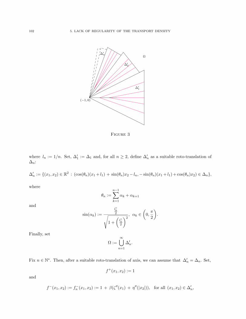
102 5. LACK OF REGULARITY OF THE TRANSPORT DENSITY
(−1, 0)
Ω
∆′1
∆′2
∆′n
Figure 3
where ln := 1/n. Set, ∆′1 := ∆1 and, for all n ≥ 2, define ∆′n as a suitable roto-translation of∆n:
∆′n := (x1, x2) ∈ R2 : (cos(θn)(x1 + l1) + sin(θn)x2− ln,− sin(θn)(x1 + l1) + cos(θn)x2) ∈ ∆n,
where
θn :=
n−1∑k=1
αk + αk+1
and
sin(αk) :=
lγk2√
1 +
(lγk2
)2, αk ∈
(0,π
2
).
Finally, set
Ω :=
∞⋃n=1
∆′n.
Fix n ∈ N∗. Then, after a suitable roto-translation of axis, we can assume that ∆′n = ∆n. Set,
f+(x1, x2) := 1
and
f−(x1, x2) := f−n (x1, x2) := 1 + β(ζ ′′(x1) + η′′(|x2|)), for all (x1, x2) ∈ ∆′n,
5.3. BV COUNTER-EXAMPLE 103
where ζ and η are the same functions which are constructed in the section 5.1. Let us de-note by σ the transport density between f+ and f−. Then, the restriction of σ to ∆′n is thetransport density σn between f+
n := 1∆′n and f−n . Indeed, for all n ∈ N∗, if Tn is an optimaltransport map from f+
n onto f−n and if un is the corresponding Kantorovich potential such thatun(−1, 0) = 0, for all n ∈ N∗, then it is not difficult to check that
T (x) := Tn(x), for a.e. x ∈ ∆′n
is an optimal transport map from f+ onto f−, and the corresponding Kantorovich potential willbe
u(x) := un(x), for all x ∈ ∆′n.
By (2.1), we infer that the restriction of σ to ∆′n is σn. Yet, by Section 5.2, we have al-ready shown that
|∇σn| ≈1
Jn,
where Jn is defined as in (5.28) on ∆n. Hence,
∞∑n=1
||∇σn||L1(∆′n) ≈∞∑n=1
∫ ln
0
∫ δ
0|∇σn(t, a)|Jn(t, a) dtda
≈∞∑n=1
ln =∞∑n=1
1
n= +∞,
where δ > 0 is small enough.
Hence, the transport density σ is not in BV (Ω). On the other hand, we will show that thetarget mass f− is in BV (R2). Using (5.33), it is easy to prove that
∞∑n=1
||∇f−n ||L1(∆′n) ≤ C∞∑n=1
(lγn + l2n) < +∞.
In addition, for a fixed n ∈ N∗ and after a suitable roto-translation of axis so that ∆′n = ∆n,we can assume that
f−n (x1, x2) = 1 + β(ζ ′′(x1) + η′′(|x2|))and,
f−n+1(x1, x2) = 1 + β
(ζ ′′(cos(θn+1)(x1 + ln) + sin(θn+1)x2 − ln+1)
+ η′′(| − sin(θn+1)(x1 + ln) + cos(θn+1)x2|))

104 5. LACK OF REGULARITY OF THE TRANSPORT DENSITY
whereθn+1 := αn + αn+1 ≈ lγn+1.
Hence, it is not difficult to check that
∣∣∣∣f−n+1
(x1,
lγn2
(x1 + ln)
)− f−n
(x1,
lγn2
(x1 + ln)
)∣∣∣∣ ≤ Cl2n.Finally, we get
∞∑n=1
∫∂∆′n∩ ∂∆′n+1
|f−n+1(z)− f−n (z)|dz ≤ C∞∑n=1
l2n < +∞.
As f− is bounded and Per(Ω) ≈∑n
(lγn+l2n) < +∞, we infer that the target mass f− ∈ BV (R2)
and the statement (5.1) follows.
5.4. Counter-examples with compactly supported smooth densities on the wholeplane
In this section, we want to show that is also possible to construct the target measure f− sothat it will be regular on R2. Firstly, let us observe that the function ζ (see Section 5.1) canbe replaced by ψζ, where ψ is a C∞ function such that ψ = 1 on [−1, 1 − ε′] and ψ = 0 on[1 − ε, 1], where 0 < ε < ε′ < 1. Let χ1, χ2 be two cut-off functions supported on ∆ ∪ R(∆),where R is the reflection map with respect to the x1-axis, such that spt(χ2) ⊂ χ1 = 1,∆a0 ∩ x : x1 ≤ 1 − ε ⊂ χ1 = 1 (where a0 ∈ (ε, 1) is such that spt(χ2) ⊂ ∆a0 ∪ R(∆a0)),∆ε ∩ x : x1 ≤ 1− ε ⊂ χ2 = 1 and χ1, χ2 are symmetric with respect to the x1-axis. Set,
f+ := χ1
and
f− := χ1 + β
(((ψζ)′′(x1) + η′′(|x2|)
)χ2 + ϕ(x1)c(a(x1, |x2|))
),
where ϕ is a non-negative C∞ function such that spt(ϕ) ⊂ (1 − ε′, 1 − ε) and c is to be de-termined in such a way that ∫
∆a
f+ =
∫∆a
f− for all a ∈ (0, 1),
which is equivalent to say that
−∫
∆a
((ψζ)′′(x1) + η′′(x2))χ2(x1, x2) dx1 dx2 =
∫∆a
ϕ(x1)c(a(x1, x2)) dx1 dx2, for all a ∈ (0, 1).
5.4. SMOOTH DENSITIES ON THE WHOLE PLANE 105
Differentiating this equality with respect to a, we get
c(a) =−∫ 1−a(γ(x1 + a) + a)((ψζ)′′(x1) + η′′(a
γ
2 (x1 + a)))χ2(x1,aγ
2 (x1 + a)) dx1∫ 1−a(γ(x1 + a) + a)ϕ(x1) dx1
, ∀ a ∈ (0, 1).
By (5.9), we have
−∫ 1
−a(γ(x1 +a)+a)(ψζ)′′(x1) dx1 =
∫ 1
−a(γ(x1 +a)+a)η′′
(aγ
2(x1 +a)
)dx1, for all a ∈ (0, 1).
Hence, for a < ε, we get
c(a) =
∫ 1−a(γ(x1 + a) + a)η′′(a
γ
2 (x1 + a))(1− χ2(x1,aγ
2 (x1 + a))) dx1∫ 1−a(γ(x1 + a) + a)ϕ(x1) dx1
and
c′(a) =1∫ 1
−a(γ(x1 + a) + a)ϕ(x1) dx1
((γ+1)
∫ 1
−aη′′(aγ
2(x1+a)
)(1−χ2
(x1,
aγ
2(x1+a)
))dx1
+aγ−1
2
∫ 1
−a(γ(x1+a)+a)2η′′′
(aγ
2(x1+a)
)(1−χ2
(x1,
aγ
2(x1+a)
))dx1−(γ+1)
(∫ 1
−aϕ(x1)dx1
)c(a)
− aγ−1
2
∫ 1
−a(γ(x1 + a) + a)2 η′′
(aγ
2(x1 + a)
)∂x2χ2
(x1,
aγ
2(x1 + a)
)dx1
).
Using (5.33), we infer that
c′(a) ≤ Ca
and,
||∇(ϕ c(a))||pLp(∆) ≈∫ 1−ε
1−ε′
∫ ε
0
(ϕ(x1)p
|c′(a)|p
J(t, a)p+|∇ϕ(x1)|p|c(a)|p
)dx2 dx1 ≈
∫ ε
0
1
a1−(γ−(γ−2)p)da.
Hence, for γ > 2,
f− ∈W 1, γγ−2−ε
(R2), for all ε > 0.
106 5. LACK OF REGULARITY OF THE TRANSPORT DENSITY
Similarly, we get that for γ = 12 : f− ∈ C∞(R2), for γ = 1 : f− ∈ C2,1(R2), for 1 < γ < 2 :
f− ∈ C1, 2γ−1
(R2) and, finally, for γ = 2 : f− ∈ C0,1(R2).

CHAPTER 6
Boundary-to-boundary transport densities, and applications tothe BV least gradient problem in 2D
The least gradient problem (minimizing the BV norm with given boundary data) is known to be equiv-
alent, in the plane, to the Beckmann minimal-flow problem with source and target measures located on
the boundary of the domain. Motivated by this fact, we prove Lp summability results for the solution
of the Beckmann problem in this setting, which improve upon previous results where the measures were
themselves supposed to be Lp. This provides results about the W 1,p regularity of the solution of the least
gradient problem in uniformly convex domains.
This chapter is taken from a joint article with F. Santambrogio, [56].
6.1. Introduction
A classical problem in calculus of variations, which is of interest both with applications inimage processing but also for its connection with minimal surfaces, is the so-called least gra-dient problem, considered for instance in [65, 94, 89, 108, 91, 12]. This is the problem ofminimizing the total variation of the vector measure ∇u among all BV functions u defined onan open domain Ω with given boundary datum. If we consider
(6.1) inf
|∇u|(Ω) : u ∈ BV (Ω), u|∂Ω = g
,
where u|∂Ω denotes the trace of u in the sense of BV functions and |∇u| denotes the totalvariation measure of ∇u, this problem relaxes into
(6.2) min
|∇u|(Ω) +
∫∂Ω|u|∂Ω − g|dHd−1 : u ∈ BV (Ω)
.
This can also be expressed in the following way: extend g into a BV function g defined ona larger domain Ω′, and then consider
(6.3) min
|∇u|(Ω) : u ∈ BV (Ω′), u = g on Ω′ \ Ω
.
107

108 6. W 1,p BOUNDS FOR THE BV LEAST GRADIENT PROBLEM IN 2D
The boundary datum g should be taken as a possible trace of BV functions, i.e. in L1(∂Ω),yet, the fact that the (a) solution u to (6.2) and (6.3) satisfies or not u|∂Ω = g could depend ong (and on the domain). In case we have u|∂Ω = g, then u is also a solution of (6.1). In [64], theauthor proves existence of solutions to (6.1) for boundary data in BV (∂Ω), while, in [106], theauthors give an example of a function g such that (6.1) has no solution (g was chosen to be thecharacteristic function of a certain fat Cantor set, which does not lie in BV (∂Ω)).
In this chapter the least gradient problem will only be considered in the planar case Ω ⊂ R2,and the boundary datum g will be at least in BV (∂Ω) (something which makes perfectly sense,since ∂Ω is a closed curve, and we are just speaking about BV functions in 1D).
Following [65], we can see that there is a one-to-one correspondence between vector measures∇u in (6.3) (considered as measures on Ω, so that we also include the part of the derivative of uwhich is on the boundary, i.e. the possible jump from u|∂Ω to g) and vector measures w satisfy-
ing, in Ω, ∇·w = f where f is the measure obtained as the tangential derivative of g ∈ BV (∂Ω);moreover, the mass of ∇u and of w are the same. Indeed, one just needs to take w = Rπ
2∇u,
where Rθ denotes a rotation with angle θ around the origin, and w solves the Beckmann problem
(6.4) inf
|w|(Ω) : w ∈M2(Ω), ∇ · w = f
,
where we denote by M2(Ω) the space of finite vector measures on Ω valued in R2. If weidentify f = ∂g/∂t (t := R−π
2n standing for the tangent vector to ∂Ω) with its restriction to the
boundary, we can also write the condition ∇ · w = f as ∇ · w = 0 in Ω, w · n = f on ∂Ω (whenwe write ∇ · w = f we mean
∫∇ϕ · dw = −
∫ϕdf for every smooth test function ϕ, without
imposing ϕ to have compact support, i.e. we also include boundary conditions).
The study of the least gradient problem can consequently be done by studying (6.4), and thequestion whether (6.1) has a solution becomes whether the solution to (6.4) gives mass to theboundary or not.
From Chapter 2, we have already seen that the Beckmann problem is strongly related to optimaltransport theory, and is in some sense equivalent to the Monge-Kantorovich problem
(6.5) min
∫Ω×Ω|x− y| dγ : γ ∈M+(Ω× Ω), (Πx)#γ = f+ and (Πy)#γ = f−
,
where f± represent the positive and negative parts of f , i.e. two positive measures with thesame mass. The scalar measure σ = |w| obtained from an optimal w is the transport density

6.2. MONGE-KANTOROVICH AND BECKMANN PROBLEMS FROM BOUNDARY TO BOUNDARY 109
(see (2.1)). Of course, Lp summability of σ is equivalent to W 1,p regularity of the optimal u.From Propositions 2.3 & 2.4, we have the following Lp summability results on the transportdensity σ: in dimension d, for p < d/(d − 1), we have w ∈ Lp as soon as at least one betweenf+ or f− is in Lp, while for general p (including p = ∞), this is proven when both f+ andf− belong to Lp(Ω). But in the case of interest for applications to the least gradient problem,the measures f± are singular (they are concentrated on the negligible set ∂Ω). The only resultobtained so far with measures concentrated on the boundary is the one that we presented inChapter 3, where we considered the case where f− is the projection of f+ on ∂Ω. On the otherhand, this is far from the setting that we want to study now, since, first, in Chapter 3, only oneof the two measures is on ∂Ω and, second, it is not an arbitrary measure but it is chosen to bethe projection of the other.
We can say that, so far, the Lp summability of w in the case where both the measures f+ andf− are concentrated on the boundary is unknown. In particular, we do not know whether theoptimal flow w belongs or not to Lp(Ω,Rd) provided f± ∈ Lp(∂Ω).
The goal of the present chapter is exactly to investigate this kind of Lp summability resultsunder suitable assumptions on the domain Ω, and then applying them to the W 1,p regularity ofthe solution of (6.1).
This chapter is organized as follows. In Section 6.2, we adapt some well known facts concerningthe usual Monge-Kantorovich problem to the precise setting of transport from the boundaryto the boundary. In Section 6.3, we show positive results on the Lp summability of σ in thetransport from a measure on the boundary to a measure on the boundary of a uniformly convexdomain, in arbitrary dimension d ≥ 2. In particular, we see that f± ∈ Lp(∂Ω) ⇒ σ ∈ Lp(Ω)holds for p ≤ 2 (to go beyond L2 summability one needs extra regularity of the data). Section6.4 gives indeed a counter-example where f ∈ L∞ but σ /∈ Lp for any p > 2. Section 6.5summarizes the applications, in the case d = 2, of these results to the least gradient problem.Finally, Section 6.6 is devoted to the study of the anisotropic case.
Many of the results that we recover were already known thanks to different methods, but webelieve that the connection with optimal transport and the technique we develop are interestingin themselves. Moreover, we believe that the following one is novel: if Ω is a uniformly convexdomain in dimension 2, p ≤ 2 and g ∈ W 1,p(∂Ω), then the solution to (6.1) exists, is unique,and belongs to W 1,p(Ω) (this is our Theorem 6.11).
6.2. Monge-Kantorovich and Beckmann problems from boundary to boundary
We begin this section by recalling that an optimal transport map T for the Monge problemfrom f+ onto f− exists as soon as f+ Ld (see Theorem 1.6). Since we are interested intransport problems where f+ is concentrared on the negligible set ∂Ω, we will see later that thesame is also true in other cases without absolutely continuous measures, and in particular in thecase of interest for us.

110 6. W 1,p BOUNDS FOR THE BV LEAST GRADIENT PROBLEM IN 2D
On the other hand, we also recall that every solution of the Beckmann problem (6.4) is ofthe form w = wγ (see (2.6)) for an optimal transport plan γ (see Proposition 2.6). As in generalProblem (6.5) can admit several different solutions, also (6.4) can have non-unique solutions.Yet, it is possible to prove that when either f+ or f− are absolutely continuous measures, thenall different optimal transport plans γ induce the same vector measure wγ ; but, this is not thecase now as both f+ and f− are concentrated on the boundary.
So, when the measures f+ and f− are concentrated on the boundary, we do not know yet,for instance, if an optimal transport map T between them exists or not, or if we have unique-ness of the transport density. Let us prove that any optimal γ in this case is induced by atransport map, which also implies uniqueness of γ and of σγ . We first start from the cased = 2, which is easier to deal with.
From now on we will suppose the condition that f+ and f− have no common mass, whichmeans that there exist two disjoint sets A+ and A− contained in ∂Ω with f± concentratedon A± (beware that these sets are not necessarily the two supports of f+ and f−).
Proposition 6.1. Suppose that Ω is strictly convex, and d = 2. Then, if f+ is atomless(i.e., f+(x) = 0 for every x ∈ ∂Ω) and f+ and f− have no common mass, there is a uniqueoptimal transport plan γ for (6.5), between f+ and f−, and it is induced by a map T .
Proof. Let γ be an optimal transport plan between f+ and f−. Let D be the set ofdouble points, that is those points whose belong to several transport rays. Take x ∈ D and letr±x be two different transport rays starting from x. Let ∆x ⊂ Ω be the region delimited by r+
x ,r−x and ∂Ω. As Ω is strictly convex, then we see easily that |∆x| > 0 and the interior parts ofall these sets ∆x, x ∈ D, are disjoint. This implies that the set D is at most countable andso f+(D) = 0 as f+ is atomless. On the other hand, for every x ∈ A+ \ D there is a uniquetransport ray rx starting from x, and this ray rx intersects A− in - at most - one point, whichwill be denoted by T (x). Hence, we get that γ = (Id, T )#f
+, which is equivalent to saying thatγ is, in fact, induced by a map T . The uniqueness follows in the usual way: if two plans γ andγ′ optimize (6.5), the same should be true for (γ + γ′)/2. Yet, for this measure to be inducedby a map, it is necessary to have γ = γ′.
The higher-dimensional counterpart of the above result should replace the assumption that f+
is atomless with the assumption that f+ gives no mass to (d− 2)-dimensional sets (i.e. sets ofcodimension 1 within the boundary). Yet, this seems more complicated to prove, and we willjust stick to an easier result, in the case where f+ is absolutely continuous w.r.t. to the Hd−1
measure on ∂Ω (that we simply write f+ ∈ L1(∂Ω)).
Proposition 6.2. Suppose that Ω is strictly convex, and d ≥ 2. Then, if f+ ∈ L1(∂Ω)and f+ and f− have no common mass, there is a unique optimal transport plan γ for (6.5),and it is induced by a map T .
6.2. MONGE-KANTOROVICH AND BECKMANN PROBLEMS FROM BOUNDARY TO BOUNDARY 111
Proof. Let γ be an optimal transport plan between f+ and f−. According to the strategyabove, it is enough to prove that for f+-a.e. x ∈ A+ there is at most a unique point y ∈ A− suchthat (x, y) ∈ spt γ. We will parametrize A± via variables s± ∈ Rd−1. This is for sure possiblesince both A± do not fill the whole boundary ∂Ω, and every proper subset of such a boundaryis homeomorphic to a subset of Rd−1, via an homeomorphism which can also be chosen to belocally bi-Lipschitz. Up to removing a negligible set, we can also assume that it is differentiableeverywhere. Under this parameterization, we face a new transport problem in Rd−1, with a newcost function c(s+, s−) := |x(s+) − y(s−)|, where s+ 7→ x(s+) and s− 7→ y(s−) are the aboveparameterization of A+ and A−.
Using standard arguments from optimal transport theory (see [103, Chapter 1]) one can seethat the Kantorovich potentials in this new transport problem are locally Lipschitz continuous,and hence differentiable a.e. Thus it is enough to check that c satisfies the twist condition toprove that γ is necessarily induced by a map T , and that it is unique. Computing the gradientof c w.r.t. the variable s+ one gets
∇s+c(s+, s−) =x(s+)− y(s−)
|x(s+)− y(s−)|Dx(s+),
where Dx(s+) is the Jacobian matrix of the diffeomorphism x. We need to prove that thisexpression is injective in s−. Having two different values of s− (say, s−0 and s−1 ) where these ex-pressions coincide means, using that s+ 7→ x(s+) is a diffeomorphism, that the two unit vectorsx(s+)− y(s−i )/|x(s+)− y(s−i )| have the same projection onto the tangent space to ∂Ω at x(s+)
(note that, from A+ ∩A− = ∅, we can assume x(s+) 6= y(s−i )). Since they are unit vectors, andthey both point to the interior of Ω, which is convex, then they should fully coincide. But thismeans that the direction connecting x(s+) to the points y(s−i ) is the same, and since all these
points lie on the boundary of a strictly convex domain, we have y(s−0 ) = y(s−1 ).
For the sake of the next section, we want stability results on the transport density. Suppose thatf+ and f− are fixed, and that a unique optimal transport plan γ exists in the transportationfrom f+ to f−. In this case we will directly write σ instead of σγ , if no ambiguity arises. Giventhe optimal transport plan γ, let us define the measure ft via
(6.6) ft = (Πt)#(|x− y| · γ)
where Πt(x, y) := (1 − t)x + ty. From (2.1), the transport density σ may be easily writtenas
σ =
∫ 1
0ft dt.
We also define a sort of partial transport density that will be useful in the sequel: given τ ≤ 1, set
112 6. W 1,p BOUNDS FOR THE BV LEAST GRADIENT PROBLEM IN 2D
(6.7) σ(τ) =
∫ τ
0ft dt.
Note that σ(τ) really depends on γ, i.e., differently from σ, it is not in general true that dif-ferent optimal plans γ induce the same σ(τ). On the other hand, we will only use this partialtransport density in cases where the optimal γ is unique. In this case we can also obtain
Proposition 6.3. Suppose f+ ∈ M+(Ω) is fixed and f−n f−. Let γn be an optimaltransport plan between f+ and f−n and suppose that there is a unique optimal transport plan
between f+ and f−. Fix τ ≤ 1 and define σ(τ)n according to (6.6) and (6.7) using γn, and σ(τ)
using γ. Then, we have σ(τ)n σ(τ).
Proof. This is a simple consequence of Proposition 1.3, of the continuity of the function(x, y) 7→ |x− y|, and of the uniqueness of the optimal γ.
6.3. Lp summability of boundary-to-boundary transport densities
In all that follows, Ω is a compact and uniformly convex domain in Rd, f+ and f− are twonon-negative Borel measures concentrated on the boundary, and at least one of them will belongto L1(∂Ω). Since we are only interested in the transport density between these two measures,we can always assume that they have no common mass, as the transport density only dependson the difference f+ − f− and common mass can be subtracted to both of them. Then, byPropositions 6.1 and 6.2, there will exist one unique optimal transport plan between these twomeasures. We will make use of the transport density σ and of σ(τ), defined in (6.7) and provideestimate on them. The main point is the following estimate.
Proposition 6.4. Suppose that the domain Ω is uniformly convex, with all its curva-tures bounded from below by a constant κ > 0, take p > 1 and f+ ∈ Lp(∂Ω). Moreover, ifp > 2 also suppose
∫f+(x)pd(x, spt(f−))2−pdHd−1(x) < +∞. Then, there exists a constant
C = C(κ,diam(Ω)) such that we have
∫Ω|σ(τ)|pdx ≤ C
(∫ τ
0
1
(1− t)(d−1)(p−1)dt
)∫∂Ωf+(x)pD(x)2−pdHd−1(x),
where D(x) := |x − T (x)| is the distance between each point x ∈ ∂Ω and its image T (x) inthe optimal transport map which induces the optimal plan γ.
Proof. Following the same strategy as in Chapter 2, we first assume that the target measuref− is finitely atomic (the points (xj)j=1,...,m being its atoms). Let T be the optimal transportmap from f+ onto f−. For all j ∈ 1, ...,m, consider T−1(xj) ⊂ ∂Ω, and partition it infinitely many smaller part, so that each can be represented by a single smooth chart parameter-izing a part of ∂Ω. We will call (χi)i=1,...,n these parts. Let us call Ωi the union of all transport
6.3. Lp SUMMABILITY OF BOUNDARY-TO-BOUNDARY TRANSPORT DENSITIES 113
rays starting from points in χi, all these rays pointing to a common point xj(i) (but we will
write xi for simplicity). Call Ω(τ)i the set of points of the form (1 − t)x + txi, with x ∈ χi
and t ≤ τ . The sets Ωi (and hence also Ω(τ)i ) are essentially disjoint (the mutual intersections
between them are Lebesgue-negligible). Set σ(τ)i := σ(τ) Ωi, for every i ∈ 1, ..., n. Of course,
σ(τ)i is concentrated on Ω
(τ)i . In order to get Lp estimates on σ(τ), we want to give an explicit
formula of each σ(τ)i . Fix i ∈ 1, ..., n and let αi be a regular function such that, up to choosing
a suitable system of coordinates, χi is contained in the graph of s 7→ αi(s), with s ∈ χi ⊂ Rd−1
(hence, the sets χi are the (d− 1)-dimensional domains where the charts are defined). For every
y ∈ Ω(τ)i , there are a unique point x = (s, αi(s)) ∈ χi and t ∈ [0, τ ] such that
y := (y′, yd) = (1− t)x+ txi = ((1− t)s+ tx′i, (1− t)αi(s) + txi,d),
where we write xi := (x′i, xi,d) by separating the last (vertical) coordinate from the others.For all ϕ ∈ C(Ωi), we get
∫Ωi
ϕ(y) dσ(τ)i (y) =
∫χi
∫ τ
0ϕ((1− t)x+ txi)|x− xi|dtdf+(x)
=
∫Ω
(τ)i
ϕ(y)|(s, αi(s))− xi| f+(s, αi(s))
√1 + |∇αi(s)|2
Ji(t, s)dy,
where Ji(t, s) := | det(D(s,t)(y′, yd))|.
Hence,
σ(τ)(y) =|(s, αi(s))− xi| f+(s, αi(s))
√1 + |∇αi(s)|2
Ji(t, s), for a.e. y ∈ Ω
(τ)i .(6.8)
Then, we have
||σ(τ)||pLp(Ω) =
n∑i=1
∫χi
∫ τ
0σ(τ)((1− t)x+ txi)
pJi(t, s) dtds
=n∑i=1
∫χi
∫ τ
0
|x− xi|pf+(x)p(1 + |∇αi(s)|2)
p−12
Ji(t, s)p−1dt dHd−1(x).
Compute
D(s,t)(y′, yd) =
((1− t)I x′i − s
(1− t)∇αi(s) xi,d − αi(s)
),

114 6. W 1,p BOUNDS FOR THE BV LEAST GRADIENT PROBLEM IN 2D
where I is the (d − 1) × (d − 1) identity matrix. Up to considering sets χi which are verysmall, each one close to a point x ∈ ∂Ω, and choosing a coordinate system where the verti-cal coordinate is parallel to the normal vector to ∂Ω at x, we can assume that ∇αi(s) is verysmall. At the limit, we can compute the above determinant as if it vanished, and thus we getJi(t, s) = (1− t)d−1(xi,d − α(s)) (as well as 1 + |∇αi(s)|2 = 1). This allows to write the change-of-variable coefficients in an intrinsic way, and thus obtain
||σ(τ)||pLp(Ω) =n∑i=1
∫χi
∫ τ
0
|x− xi|pf+(x)p
(1− t)(d−1)(p−1)((xi − x) · n(x)
)p−1 dtdHd−1(x),
where n(x) is the inward normal vector to ∂Ω at x. Using the lower bound on the curva-ture of ∂Ω we have, for every pair of points x and xi on ∂Ω:
(xi − x) · n(x) ≥ c|x− xi|2,
for a constant c = c(diam Ω, κ). Using then xi = T (x) for x ∈ χi, this provides the desiredformula
||σ(τ)||pLp(Ω) ≤ C∫∂Ω
∫ τ
0
|x− T (x)|2−pf+(x)p
(1− t)(d−1)(p−1)dtdHd−1(x).
This gives the desired result when f− is atomic. If not, take a sequence (f−n )n of atomicmeasures converging to f− and concentrated on spt(f−). Call Tn the optimal maps from f+ to
f−n and Dn(x) = |x−Tn(x)|. By Proposition 6.3, the partial transport densities σ(τ)n converge to
the corresponding partial transport density σ(τ) and by Proposition 1.3 the optimal transportmaps Tn also converge a.e. to the optimal transport map T inducing γ (up to extracting a sub-sequence, since L2(f+) convergence implies a.e. convergence up to a subsequence). Moreover,we have
∫∂ΩDn(x)2−pf+(x)
pdHd−1(x) →
∫∂ΩD(x)2−pf+(x)
pdHd−1(x) by dominated conver-
gence, using either p ≤ 2 and f+ ∈ Lp(∂Ω) or∫∂Ω d(x, spt(f−))2−pf+(x)
pdHd−1(x) < +∞,
according to our assumptions. Using semicontinuity on the left hand side, we get
||σ(τ)||pLp(Ω) ≤ lim infn||σ(τ)
n ||pLp(Ω) ≤ C
(∫ τ
0
1
(1− t)(d−1)(p−1)dt
)∫∂ΩD(x)2−pf+(x)
pdHd−1(x)
and the result is proven in general.
From the above estimate, we can deduce many integrability results.

6.3. Lp SUMMABILITY OF BOUNDARY-TO-BOUNDARY TRANSPORT DENSITIES 115
Proposition 6.5. Suppose d ≥ 2 and f+ ∈ Lp(∂Ω) with p < d/(d− 1). Then, the trans-port density σ between f+ and any f− ∈M+(∂Ω) is in Lp(Ω).
Proof. Note that our assumption on p implies p < 2. To prove this result it is enough to
use Proposition 6.4 with τ = 1, since in this case the integral∫ 1
01
(1−t)(d−1)(p−1) dt converges, and
the term D(x)2−p is bounded.
Proposition 6.6. Suppose that f+, f− ∈ Lp(∂Ω) with p ≤ 2. Then, the transport densityσ between these two measures is in Lp(Ω).
Proof. In this case the integral in the estimate of σ = σ(τ) with τ = 1 diverges, so weneed to adapt our strategy. Following again Chapter 2, we write
σ = σ+ + σ−,
where σ+ = σ(1/2) and σ− = σ − σ(1/2). In this case the Lp summability of f+ guarantees thatof σ+ since p ≤ 2 implies that D(x)2−p is bounded. Symmetrically, the Lp summability of f−
guarantees that of σ−. Note that, thanks to Propositions 6.1 and 6.2, we do not face the samedifficulties as in Chapter 2, where it was not obvious to glue together estimates on σ+ obtainedby approximating f− and estimates on σ− coming from the approximation of f+.
We will see in Section 6.4 that the same result is false for p > 2, and that in order to obtainhigher integrability we need to assume much more on f+ and f−.
Remark 6.7. We do not discuss it here in details, but the summability result also worksfor Orlicz spaces with growth less than quadratic, i.e. we have, for every convex and superlinearfunction Ψ = R+ 7→ R+ with Ψ(s) ≤ C(s2 + 1),
∫Ω
Ψ(σ(x))dx ≤ C∫∂Ω
Ψ(|f(x)|)dHd−1(x) + C.
This can be proven in similar ways with suitable manipulations on the function Ψ. In par-ticular, this implies that f ∈ L1(∂Ω)⇒ σ ∈ L1(Ω).
Proposition 6.8. Suppose that f+, f− ∈ C0,α(∂Ω) for 0 < α ≤ 1. Then, the transportdensity σ between these two measures is in Lp(Ω) for p = 2/(1− α) (with p =∞ for α = 1).
Proof. First, we check that we can apply Proposition 6.4, since in this case we need touse p = 2/(1 − α) > 2. Consider a point x with f+(x) > 0, and take a point y ∈ spt(f−)with |x − y| = d(x, spt(f−)). Then we have f+(y) = 0 (since f+ and f− have no mass incommon) and f+(x) = |f+(x) − f+(y)| ≤ C|x − y|α. This provides d(x, spt(f−))2−pf+(x)
p ≤Cd(x, spt(f−))2−p+pα. With our choice of p, this quantity is bounded since the exponent is non-negative (for α < 1 the choice p = 2/(1−α) provides a zero exponent; for α = 1 this exponent

116 6. W 1,p BOUNDS FOR THE BV LEAST GRADIENT PROBLEM IN 2D
is equal to 2 for any p). This in particular guarantees∫∂Ω d(x, spt(f−))2−pf+(x)
pdHd−1(x) <
+∞. Of course, the same can be performed on f−. Then, the same strategy as in Proposition6.6 shows
||σ||pLp(Ω) ≤ C(∫
∂Ω|D(x)|2−pf+(x)
pdHd−1(x) +
∫∂Ω|D−(x)|2−pf−(x)
pdHd−1(x)
),
where D−(x) := |x−T−1(x)| is defined as D(x), but relatively to f−. Using D(x) = |x−T (x)| ≥d(x, spt(f−)), the quantity D(x)2−pf+(x)
p ≤ CD(x)2−p+pα is bounded. Since a similar argu-ment can be performed on f−, we obtain finiteness of the norm ||σ||Lp(Ω) (and for α = 1 weobtain σ ∈ L∞ by passing to the limit p→∞).
6.4. Counter-example to the L2+ε summability
In this section, we show that the Lp estimates for the transport density, in the case wherep > 2, fail even if we assume f± ∈ L∞(∂Ω). More precisely, we will construct an example of f±,where f± ∈ L∞(∂Ω), but the transport density σ between them does not belong to L2+ε(Ω) forany ε > 0. For simplicity, this will be done in dimension d = 2.
Let Ω be a disk and let (χ±n )n be a sequence of arcs in ∂Ω such that H1(χ±n ) = εn, forsome sequence εn to be chosen later. We will put these arcs one after the other, so that theyonly have endpoints in common, and we assume that they are ordered in the following way:χ+n−1, χ
−n−1, χ
−n , χ
+n , χ
+n+1, χ
−n+1, for all n (see Figure 1).
χ+n−1
χ−n−1
χ−n
χ+n
χ+n+1
χ−n+1
∆n
Figure 1
Set f± = 1χ± , where χ± = ∪nχ±n , and let T be the optimal transport map from f+ to f−.
Correspondingly, let σ be the transport density. We see easily that the restriction of T to χ+n
is the optimal transport map Tn between f+n and f−n , where f±n is the restriction of f± to χ±n .
Moreover, if we denote by ∆n the union of all transport rays from f+n onto f−n , then the restric-
tion of the transport density σ to ∆n is the transport density σn between f+n and f−n . We want
to compute this density σn. Let s 7→ αn(s) be a parameterization of χ+n ∪χ−n where s = 0 corre-
sponds to the boundary point between the two arcs. It is clear that Tn(s, αn(s)) = (−s, αn(s)),
6.4. COUNTER-EXAMPLE TO THE L2+ε SUMMABILITY 117
for all s ∈ [0, εn]. Then, for every y ∈ ∆n, there is a unique (t, s) ∈ [0, 1]× [0, εn] such that
y := (y1, y2) = (1− t)(s, αn(s)) + t(−s, αn(s)) = ((1− 2t)s, αn(s)).
Hence, for every ϕ ∈ C(∆n), we have
∫∆n
ϕ(y)σn(y) dy =
∫χ+n
∫ 1
0ϕ((1− t)x+ tTn(x))|x− Tn(x)|f+
n (x) dtdx
=
∫ εn
0
∫ 1
0ϕ((1− 2t)s, αn(s)) 2s
√1 + α ′n(s)2 dt ds
=
∫∆n
ϕ(y)2s√
1 + α ′n(s)2
Jn(t, s)dy,
where Jn(t, s) := |det(D(t,s)(y1, y2))| on ∆n.
Then, we get
σn(y) =2s√
1 + α ′n(s)2
Jn(t, s), for a.e. y ∈ ∆n.
Consequently, we obtain
||σ||pLp(Ω) =
∞∑n=1
∫ εn
0
∫ 1
0σn((1− 2t)s, αn(s))pJn(t, s) dt ds
≈∞∑n=1
∫ εn
0
∫ 1
0
sp
Jn(t, s)p−1dt ds.
Computing
D(t,s)(y1, y2) =
(−2s 1− 2t
0 α ′n(s)
),
we get
Jn(t, s) = 2s α ′n(s) ≈ s2.

118 6. W 1,p BOUNDS FOR THE BV LEAST GRADIENT PROBLEM IN 2D
Finally, we have
||σ||pLp(Ω) ≈∞∑n=1
ε3−pn .
This immediately shows that with this construction we cannot have σ ∈ L3. Moreover, itis enough to choose a sequence εn satisfying
∞∑n=1
εn < +∞,∞∑n=1
εβn = +∞
for all β < 1, to prove σ /∈ Lp(Ω) for all p > 2. Take for instance εn = 1n(log(1+n))2 .
6.5. Applications to the BV least gradient problem
We collect in this section some corollaries of the results of the previous sections, which giveinteresting proofs for some properties of the BV least gradient problem in dimension d = 2.We need to restrict to d = 2 because only in this framework rotated gradients have prescribeddivergence.
In all the cases, we will suppose g ∈ BV (∂Ω). Note that this assumption is required to ap-ply the classical theory of optimal transport to f = ∂tg; this requires to transport a measureonto another. If g was only in L1(∂Ω), then f would be the (one-dimensional) derivative of anL1 function, i.e. an element of the dual of Lipschitz functions (since W−1,1 = (W 1,∞)′). It isnot surprising that a Monge-Kantorovich theory is also possible in this case (because formula(1.2) characterizes the transport cost as the dual norm to the Lipschitz norm), see [16], but noestimates are possible.
Proposition 6.9. If Ω ⊂ R2 is strictly convex and g ∈ BV (∂Ω), then Problem (6.1) has asolution (i.e. Problems (6.2) and (6.3) have a solution whose trace is g).
Proof. We have already discussed the fact that we just need to exclude that the solutionof (6.2) or (6.3) has a part of its distributional derivative on the boundary. After the rotation,this means that its trace agrees with g if and only if σ(∂Ω) = 0. Yet, in strictly convex domains,the transport density does not give mass to the boundary, because of the representation formula(2.2).
Proposition 6.10. If Ω ⊂ R2 is strictly convex, and g ∈ (BV ∩ C0)(∂Ω), then Problem(6.1) has a unique solution.
Proof. Using again the rotation trick, we just need to prove uniqueness of the transportdensity. The condition g ∈ C0 implies that its tangential derivative has no atoms, and we can
6.5. APPLICATIONS TO THE BV LEAST GRADIENT PROBLEM 119
apply Proposition 6.1.
The following result is probably the main contribution of this chapter to the understanding ofthe least gradient problem, as we are not aware of similar results already existing in the literature.
Theorem 6.11. If Ω ⊂ R2 is uniformly convex, and g ∈ W 1,p(∂Ω) with p ≤ 2, then theunique solution of Problem (6.1) belongs to W 1,p(Ω).
Proof. Setting f = ∂tg and using f+ and f− as its positive and negative parts, the condi-tion g ∈ W 1,p(∂Ω) implies f± ∈ Lp(∂Ω). Hence, Proposition 6.6 implies σ ∈ Lp(Ω), and then∇u ∈ Lp(Ω,R2).
Proposition 6.12. Even if Ω ⊂ R2 is a disk, for every p > 2 there exists g ∈ Lip(∂Ω) suchthat the unique u solution of Problem (6.1) is not in W 1,p(Ω).
Proof. It is enough to take g as the antiderivative of the function f = f+ − f− of thecounter-example of Section 6.4.
Proposition 6.13. If Ω ⊂ R2 is uniformly convex, and g ∈ C1,α(∂Ω) with α < 1, then theunique solution of Problem (6.1) belongs to W 1,p(Ω) for p = 2/(1− α).
Proof. This is a consequence of Proposition 6.8.
Remark 6.14. Note that the above W 1,p regularity also implies Holder bounds, since indimension d = 2 we have W 1,p ⊂ C0,1−2/p. In particular, using p = 2/(1 − α), we getg ∈ C1,α(∂Ω) ⇒ u ∈ C0,α(Ω). Yet, this bound is not optimal, as it is known (see, for in-
stance, [108]) that we have g ∈ C1,α(∂Ω)⇒ u ∈ C0,(α+1)/2(Ω). It is interesting to note that one
would obtain exactly the desired C0,(α+1)/2 behavior if it was possible to use the Sobolev injectionof W 1,p corresponding to dimension 1 instead of dimension 2. This seems reasonable, using thefact that level lines of u are transport rays in the transport problem from f+ to f−, hence areline segments, but it is not easy to justify and goes beyond the scopes of this chapter.
Proposition 6.15. If Ω ⊂ R2 is uniformly convex, and g ∈ C1,1(∂Ω), then the uniquesolution of Problem (6.1) is Lipschitz continuous.
Proof. This is also a consequence of Proposition 6.8.
Remark 6.16. Note that the above Lipschitz result is optimal, and perfectly coherent withthe theory involving the bounded slope condition (see, for instance [107, 41]), since C1,1 func-tions on the boundary of uniformly convex domains satisfy the bounded slope condition (see [66]).
We finish this section with the following last remark.
120 6. W 1,p BOUNDS FOR THE BV LEAST GRADIENT PROBLEM IN 2D
Remark 6.17. We observe that we have not used Proposition 6.5 in this Section. Indeed,in the framework of the least gradient problem assuming assumptions on f+ (i.e. on the posi-tive part of the tangential derivative of the boundary datum) are not natural at all. Proposition6.5 has been inserted in Section 6.3 just because it was an easy consequence of Proposition 6.4.Also consider that a simple result which could have been proven in Section 6.3 was the impli-cation f± ∈ Lp(∂Ω) ⇒ σ ∈ Lp(Ω) for arbitrary p (including p > 2) under the assumptionspt(f+) ∩ spt(f−) = ∅, but we did not considered it because this assumption, in terms of g, isvery innatural: it would mean that g has some flat regions separating those with positive andnegative derivatives.
6.6. Anisotropic least gradient problem
This section is devoted to the anisotropic least gradient problem [64, 88]. We will showbriefly that all our analysis could be done by replacing the Euclidean norm with another strictlyconvex one. Let ϕ be a given norm in R2. So, we consider the following problem
(6.9) inf
∫Ωϕ(∇u) : u ∈ BV (Ω), u|∂Ω = g
,
where∫
Ω ϕ(∇u) =∫
Ω ϕ(νu(x)) d|∇u| (νu is the Radon-Nikodym derivative νu = d∇ud|∇u|) and
g ∈ BV (∂Ω) is a given boundary datum. On the other hand, let || · || be the rotation-norm ofϕ, i.e., ||ξ|| := ϕ(R−π
2ξ), for every ξ ∈ R2. Recalling Section 6.1, we can see that the problem
(6.9) is equivalent to the following one
(6.10) inf
||w||(Ω) : w ∈M2(Ω), ∇ · w = f
,
where we denote by ||w|| the variation measure associated with the vector measure w, andf = ∂g/∂t. More precisely, if u is a solution for (6.9), then w = Rπ
2∇u solves (6.10) and, we
have ||w||(Ω) =∫
Ω ϕ(∇u).
From Section 2.3, we have already seen that the problem (6.10) is also equivalent to the Monge-Kantorovich problem, with c(x, y) = ||x− y|| as a transport cost,
(6.11) min
∫Ω×Ω||x− y||dγ : γ ∈M+(Ω× Ω), (Πx)#γ = f+ and (Πy)#γ = f−
,
where f± represent the positive and negative parts of f . In addition, we showed in Propo-sition 2.6 that if the norm ϕ (or equivalently, || · ||) is strictly convex, then any optimal flow wof (6.10) comes from an optimal transport plan γ for (6.11), i.e., w = wγ (see (2.6)).

6.6. ANISOTROPIC LEAST GRADIENT PROBLEM 121
Moreover, as soon as f+ is atomless, f+ and f− have no common mass, and Ω is strictly convex,one can prove, exactly as in Proposition 6.1, that there is a unique optimal transport plan γfor (6.11), between f+ and f−, and it is induced by a map T . This also gives the uniquenessof the solution for (6.9).
Hence, it suffices to give Lp estimates on the transport density a := ||w||, where w is theunique minimizer of (6.10), to get W 1,p estimates on the unique solution u of (6.9). Let T bethe optimal transport map between f+ and f−. Recalling (2.8), the transport density a maybe easily written as
a =
∫ 1
0ft dt,
whereft = (Tt)#(||x− T (x)|| · f+)
andTt(x) := (1− t)x+ tT (x).
Again, for every τ ≤ 1, we define
a(τ) =
∫ τ
0ft dt.
Following the same lines of the proof of Proposition 6.4, one can prove, using the fact that|| · || ≈ | · |, the following estimate∫
Ω|a(τ)|pdx ≤ C
(∫ τ
0
1
(1− t)(p−1)dt
)∫∂Ω
||x− T (x)||p
|x− T (x)|2(p−1)f+(x)p dHd−1(x)
≈ C
(∫ τ
0
1
(1− t)(p−1)dt
)∫∂Ω|x− T (x)|2−pf+(x)p dHd−1(x).
Recalling also Proposition 6.6, we conclude that the transport density a is in Lp(Ω) as soonas f± ∈ Lp(∂Ω) with p ≤ 2 and Ω is uniformly convex. Moreover, if f+, f− ∈ C0,α(∂Ω)for 0 < α ≤ 1, then the transport density a between these two measures is in Lp(Ω) forp = 2/(1− α) (with p =∞ for α = 1).
In terms of W 1,p regularity for the solution u of (6.9), we infer that u is in W 1,p(Ω) assoon as g ∈ W 1,p(∂Ω) with p ≤ 2 and Ω is uniformly convex. In addition, if g ∈ C1,α(∂Ω),
then u is in W 1, 21−α (Ω), for 0 < α ≤ 1.


CHAPTER 7
Exit-time optimal control problems
The control problems considered in this chapter will be called “exit-time” because the terminal time of
the trajectories is not fixed, but it is the first one at which they reach a given target set. A typical example
is the minimum time problem, where one wants to steer a point to the target in minimal time under some
constraints on the dynamic. It is interesting to observe that the distance function can be regarded as the
value function of a particular minimum-time problem, and so the properties of the distance function may
serve as a guideline for the analysis of the general case. We first study the existence of optimal controls;
then we introduce the value function, show that it solves a Hamilton-Jacobi equation, give a result about
its Lipschitz continuity, analyze the optimality conditions and the properties of optimal trajectories and
prove that the value function is differentiable along optimal trajectories, except possibly their endpoints.
Finally, we prove the semi-concavity of the value function, with respect to x, under much weaker assump-
tions, on the smoothness of the dynamic with respect to time, than those in [37]. Some statements in
this chapter will be similar to those in [37], even if they are stated, here, in the non-autonomous case.
But anyway, the differentiability property and the sharp semi-concavity of the value function seem to be
novel.
The original results in this chapter will be included in a joint paper with G. Mazanti,in preparation, [57].
7.1. Definition, existence and first properties
We begin by giving the definition of the control systems we are interested in.
Definition 7.1. The control system, we are interested in, consists of a pair (k, U), whereU ⊂ Rd is a compact set and k : R+ × Rd 7→ R+ is a continuous function. The set U is calledthe control set, while k is called the dynamic of the system. The state equation associated withthe system is
(7.1)
γ′(t) = k(t, γ(t))u(t), for a.e. t ≥ t0,γ(t0) = x,
where t0 ∈ R+, x ∈ Rd and u : [t0,∞) 7→ U is a measurable function (which is called acontrol). We denote the solution of (7.1) by γt0,x,u and we call it the trajectory of the systemcorresponding to the initial condition γ(t0) = x and to the control u.
Of course, this is only a very particular example of control system, but it is the simplest onewhich allows to study interesting exit time problems. In order to assume that the maximal speedof the trajectory γt0,x,u is bounded by the dynamic k, we take the control set U = B(0, 1).
123
124 7. EXIT-TIME OPTIMAL CONTROL PROBLEMS
Moreover, we list some basic assumptions on the dynamic k:
0 < kmin := inf k ≤ kmax := sup k < +∞,(7.2)
|k(t, x1)− k(t, x2)| ≤ Lx |x1 − x2|, for all x1, x2 ∈ Rd and t ∈ R+.(7.3)
Notice that the assumption (7.3) ensures the existence of a unique global solution to the stateequation (7.1) for any choice of t0, x and u. Let Ω be a bounded domain in Rd: for a giventrajectory γ = γt0,x,u of the system, we set
τ t0,x,u = infτ ≥ 0 : γt0,x,u(t0 + τ) ∈ ∂Ω,
with the convention τ t0,x,u = +∞ if γt0,x,u(t0 + τ) /∈ ∂Ω for all τ ∈ [0,∞). This meansthat we use ∂Ω as a target. We call τ t0,x,u the exit-time of the trajectory. If τ t0,x,u < +∞, weset for simplicity
γt0,x,uτ := γt0,x,u(t0 + τ t0,x,u)
to denote the point where the trajectory reaches the target ∂Ω. As kmin > 0, one can seeeasily that, for all x ∈ Ω and at each time t0 ∈ R+, there is always some control u such thatτ t0,x,u < +∞.
An optimal control problem consists of choosing the control strategy u in the state equation(7.1) in order to minimize a given functional. Let g : ∂Ω 7→ R+ be a given continuous function.At each time t0 ∈ R+ and for any initial point x ∈ Ω, we minimize the following quantity
(7.4) τ t0,x,u + g(γt0,x,uτ )
among all controls u. A control u and the corresponding trajectory γt0,x,u are called optimalfor the point x at time t0 if u minimizes (7.4). Now, suppose that
(7.5) |g(x)− g(y)| ≤ λ|x− y|, for all x, y ∈ ∂Ω
with λ < 1kmax
. We note that this assumption is similar to the one in the problem studied
in Chapter 4. Then, under the assumptions (7.2), (7.3) and (7.5), we have the following exis-tence result.

7.1. DEFINITION, EXISTENCE AND FIRST PROPERTIES 125
Proposition 7.2. For each time t0 ∈ R+ and for any initial point x ∈ Ω, there exists anoptimal control u for (7.4).
Proof. Let (un)n be a minimizing sequence. We set for simplicity τn := τ t0,x,un , γn :=
γt0,x,un and zn := γt0,x,unτn . As g is continuous on ∂Ω, then (τn)n is bounded and, up to asubsequence, τn converges to some τ . For each n ∈ N, we can assume that un(t) = 0 for allt > t0 + τn. In this way, we get that γn converges uniformly to some γ ∈ Lip([t0,∞),Ω) with|γ′| ≤ kmax. In addition, for a.e. t ∈ (t0,+∞), we have
|γ′n(t)| ≤ k(t, γn(t)).
Letting n→ +∞, we infer that |γ′(t)| ≤ k(t, γ(t)), for a.e. t ∈ (t0,+∞), which is equivalent tosay that there is some control u such that γ is the associated trajectory to u with initial pointx, at time t0. On the other hand, we have
zn → γ(t0 + τ),
which implies that γ(t0 + τ) ∈ ∂Ω and τ := τ t0,x,u ≤ τ . Yet, it is not possible to have τ < τ .Indeed, one has
limnτn + g(zn) = τ + g(γ(t0 + τ)) ≤ τ + g(γ(t0 + τ)),
which is a contradiction, as g is λ−Lipschitz with λ < 1/kmax. Thus, we have τ = τ andthis completes the proof that γ is an optimal trajectory and u is the associated optimal con-trol.
Remark 7.3. The condition that g is λ−Lip with λ < 1kmax
is crucial for this result.
Without this condition, one should replace τ + g(γ(τ)) with inft+ g(γ(t)) : γ(t) ∈ ∂Ω.
The value function of the problem is defined by
(7.6) ϕ(t0, x) = minτ t0,x,u + g(γt0,x,uτ ) : u is a control , t0 ∈ R+, x ∈ Ω.
The first important fact is that the value function ϕ satisfies the so-called dynamic programmingprinciple:
Lemma 7.4. For any t0 ∈ R+, x ∈ Ω and u : [t0,∞) 7→ B(0, 1) a control, we have
ϕ(t0, x) ≤ t− t0 + ϕ(t, γt0,x,u(t)), for all t ∈ [t0, t0 + τ t0,x,u],
with equality if u is optimal.

126 7. EXIT-TIME OPTIMAL CONTROL PROBLEMS
Proof. Let u be a control for x, at time t0, and fix t ∈ [t0, t0 + τ t0,x,u]. Set y = γt0,x,u(t)and let v be an optimal control for y at time t, i.e., we have
ϕ(t, γt0,x,u(t)) = τ t,y,v + g(γt,y,vτ ).
Let us now define the control w as follows
w(s) :=
u(s) if s ∈ [t0, t)
v(s) if s ≥ t.
Therefore, one has
γt0,x,w(s) =
γt0,x,u(s) if s ∈ [t0, t)
γt,y,v(s) if s ≥ tand,
ϕ(t0, x) ≤ τ t0,x,w + g(γt0,x,wτ ) = t− t0 + τ t,y,v + g(γt,y,vτ ).
Moreover, if the control u is optimal, then we get
ϕ(t, γt0,x,u(t)) ≤ τ t,y,u + g(γt,y,uτ ) = τ t0,x,u + t0 − t+ g(γt0,x,uτ ) = ϕ(t0, x) + t0 − t.
Now, we want to show that the value function ϕ is a viscosity solution of a suitable partialdifferential equation. In fact, we have the following classical result that we prove for complete-ness.
Proposition 7.5. The value function ϕ is a viscosity solution of the following Hamilton-Jacobi equation
(7.7) − ∂tϕ(t, x) + k(t, x) |∇xϕ(t, x)| − 1 = 0, (t, x) ∈ R+ ×Ω.
Moreover, one has ϕ(t, x) = g(x) for every (t, x) ∈ R+ × ∂Ω.
Proof. First, we prove that ϕ is a viscosity subsolution of (7.7). Let (t0, x0) ∈ R+ ×Ω
and φ be a C1 function such that φ(t0, x0) = ϕ(t0, x0) and φ(t, x) ≥ ϕ(t, x) for (t, x) in aneighborhood of (t0, x0). Fix v ∈ Rd with |v| = 1. Let us consider the trajectory γv startingfrom x0, at time t0, and corresponding to the constant control v. Hence, by Lemma 7.4, onehas, for h > 0 small enough, that
φ(t0, x0) = ϕ(t0, x0) ≤ h+ ϕ(t0 + h, γv(t0 + h)) ≤ h+ φ(t0 + h, γv(t0 + h))
and so,
0 ≤ h+ h ∂tφ(t0, x0) +
∫ t0+h
t0
γ′v(t) dt · ∇xφ(t0, x0) + o
(h+
∣∣∣∣∫ t0+h
t0
γ′v(t) dt
∣∣∣∣)

7.1. DEFINITION, EXISTENCE AND FIRST PROPERTIES 127
≤ h+ h ∂tφ(t0, x0) + (∇xφ(t0, x0) · v)
∫ t0+h
t0
k(t, γv(t)) dt+ o(h).
Thus, dividing by h and letting it to 0, one concludes that
1 + ∂tφ(t0, x0) + k(t0, x0)(∇xφ(t0, x0) · v) ≥ 0
and, since v is arbitrary, we then obtain
−∂tφ(t0, x0) + k(t0, x0) |∇xφ(t0, x0)| ≤ 1.
Let us now prove that ϕ is a viscosity supersolution of (7.7). Let (t0, x0) ∈ R+ ×Ω and φ be a
C1 function such that φ(t0, x0) = ϕ(t0, x0) and φ(t, x) ≤ ϕ(t, x) for (t, x) in a neighborhood of(t0, x0). Let γ be an optimal trajectory for x0 at time t0. Using Lemma 7.4, for h > 0 smallenough, we have
φ(t0, x0) = ϕ(t0, x0) = h+ ϕ(t0 + h, γ(t0 + h)) ≥ h+ φ(t0 + h, γ(t0 + h)),
which implies that,
0 ≥ h+ h ∂tφ(t0, x0) +
∫ t0+h
t0
γ′(t) dt · ∇xφ(t0, x0) + o
(h+
∣∣∣∣∫ t0+h
t0
γ′(t) dt
∣∣∣∣)
≥ h+ h ∂tφ(t0, x0)− |∇xφ(t0, x0)|∫ t0+h
t0
k(t, γ(t)) dt+ o(h).
Thus, again dividing by h and letting it to 0, one concludes that
−∂tφ(t0, x0) + k(t0, x0) |∇xφ(t0, x0)| ≥ 1,
proving that ϕ is a viscosity supersolution of (7.7) on R+ ×Ω. Finally, the fact that ϕ(t, x) =
g(x), for all (t, x) ∈ R+ × ∂Ω, follows immediately by using the assumption (7.5).
We denote by D+ϕ the superdifferential of ϕ, i.e., for every (t, x) ∈ R+ × Ω,
D+ϕ(t, x) :=
(h, p) ∈ R× Rd : lim sup
(s,y)→(t,x)
ϕ(s, y)− ϕ(t, x)− (h, p) · (s− t, y − x)
|(s− t, y − x)|≤ 0
.
If we consider points along optimal trajectories different from the endpoints, we can provethat the elements of D+ϕ satisfy also (7.7). So, the following result holds.
Proposition 7.6. Let γ : [t0, t0 + τ0] 7→ Ω be an optimal trajectory for x0, at time t0,where τ0 = τ t0,x0,u; u being the associated optimal control. Then, for any t ∈ (t0, t0 + τ0), wehave
−pt + k(t, γ(t)) |px| − 1 = 0, for all (pt, px) ∈ D+ϕ(t, γ(t)).
128 7. EXIT-TIME OPTIMAL CONTROL PROBLEMS
Proof. Let us take t ∈ (t0, t0 + τ0). We already know from the previous proof that
−pt + k(t, γ(t)) |px| − 1 ≤ 0, for all (pt, px) ∈ D+ϕ(t, γ(t)).
So, it suffices to prove that the converse inequality also holds. First, we observe that, by thedynamic programming principle,
ϕ(t, γ(t)) = ϕ(t− h, γ(t− h))− h, 0 ≤ h ≤ t− t0.
On the other hand, if (pt, px) ∈ D+ϕ(t, γ(t)), we have
ϕ(t− h, γ(t− h))− ϕ(t, γ(t)) ≤ −pth− px · (γ(t)− γ(t− h)) + o(h).
Therefore, we find that
0 ≤ −pth− px · (γ(t)− γ(t− h))− h+ o(h)
= −pth−∫ t
t−hk(s, γ(s)) px · u(s) ds− h+ o(h)
≤ −pth+
∫ t
t−hsup
s∈[t−h,t]k(s, γ(s)) |px|ds− h+ o(h)
≤ h(−pt + sups∈[t−h,t]
k(s, γ(s)) |px| − 1) + o(h),
which yields the conclusion.
Let us define now the minimum time function as follows:
T (t, x) = infτ t,x,u : u is a control, (t, x) ∈ R+ × Ω.
An optimal control u in T (t, x) will be called time-optimal control. Notice that we have thefollowing
Lemma 7.7. For every (t, x) ∈ R+ × Ω, one has T (t, x) ≤ k−1min d(x, ∂Ω).
Proof. Let γ be a geodesic (which is just a segment) from x to the boundary ∂Ω with|γ′| = 1. Set γ(s) = γ(kmin(s − t)), for all s ∈ [t, t + k−1
min d(x, ∂Ω)]. It is clear that γ is anadmissible trajectory, which means that there is a control u such that γ = γt,x,u. Hence, bydefinition of T , we infer that T (t, x) ≤ τ t,x,u = k−1
min d(x, ∂Ω).
In addition, one can also show that the exit-time of an optimal control for (7.4) can be estimatedby the minimum time function T . More precisely, we have the following
7.1. DEFINITION, EXISTENCE AND FIRST PROPERTIES 129
Proposition 7.8. For every (t, x) ∈ R+ ×Ω, if u is an optimal control for (7.4), then onehas
τ t,x,u ≤ 1 + λkmax
1− λkmaxT (t, x).
Proof. Let u be an optimal control for (7.4) and v be a minimal-time control for (t, x).Then, we have
τ t,x,u + g(γt,x,uτ ) ≤ τ t,x,v + g(γt,x,vτ )
and so,
τ t,x,u ≤ τ t,x,v + λ|γt,x,vτ − γt,x,uτ | ≤ τ t,x,v + λkmax(τ t,x,v + τ t,x,u).
Consequently, we get
τ t,x,u ≤ 1 + λkmax
1− λkmaxτ t,x,v =
1 + λkmax
1− λkmaxT (t, x).
Now, we want to give a result about the Lipschitz continuity of the value function ϕ. To dothat, we will, first, introduce the following estimates on the trajectories, which will be repeatedlyused in our analyis.
Proposition 7.9. For every x0, x1 ∈ Ω and t0, t ∈ R+, there exists c := c(t− t0) > 0 suchthat
|γt0,x0,u(t)− γt0,x1,u(t)| ≤ c|x0 − x1|
for all controls u : [t0,∞) 7→ B(0, 1).
Proof. We have, by (7.3), that
|γt0,x0,u(t)− γt0,x1,u(t)| =
∣∣∣∣x0 − x1 +
∫ t
t0
(k(s, γt0,x0,u(s))− k(s, γt0,x1,u(s)))u(s) ds
∣∣∣∣≤ |x0 − x1| + Lx
∫ t
t0
|γt0,x0,u(s)− γt0,x1,u(s)| ds.
Using Gronwall’s inequality, we get
|γt0,x0,u(t)− γt0,x1,u(t)| ≤ c |x0 − x1|.
Now, we are ready to prove the following

130 7. EXIT-TIME OPTIMAL CONTROL PROBLEMS
Proposition 7.10. Let our system satisfy properties (7.2), (7.3) & (7.5). Then, the valuefunction ϕ is Lipschitz continuous in R+ × Ω.
Proof. Take x0, x1 ∈ Ω and t ∈ R+. Suppose, without loss of generality, that ϕ(t, x0) ≤ϕ(t, x1). Let u be an optimal control for x0 at time t. First, assume that τ0 := τ t,x0,u ≤ τ t,x1,u.Set y0 := γt,x0,u(t+ τ0) and y1 := γt,x1,u(t+ τ0). Then, by the dynamic programming principle(see Lemma 7.4), we have
ϕ(t, x1)− ϕ(t, x0) ≤ ϕ(t+ τ0, y1)− g(y0).
Now, let v be a time-optimal control for y1, at time t+ τ0. Then, using Lemma 7.7, we get
ϕ(t, x1)− ϕ(t, x0) ≤ T (t+ τ0, y1) + g(γt+τ0,y1,vτ ) − g(y0)
≤ k−1min d(y1, ∂Ω) + λ|γt+τ0,y1,v
τ − y0|
≤ k−1min |y1 − y0| + λ|γt+τ0,y1,v
τ − y0|.Since
|γt+τ0,y1,vτ − y0| ≤ |γt+τ0,y1,v
τ − y1| + |y1 − y0|
≤ kmax T (t+ τ0, y1) + |y0 − y1|
≤(
1 +kmax
kmin
)|y0 − y1|,
we conclude, from Proposition 7.9, that
|ϕ(t, x1)− ϕ(t, x0)| ≤ c|y0 − y1| ≤ c|x0 − x1|.
If τ t,x1,u < τ0: we have
ϕ(t, x1)− ϕ(t, x0) ≤ τ t,x1,u + g(γt,x1,uτ )− τ t,x0,u − g(y0)
≤ τ t,x1,u − τ0 + λ |γt,x1,uτ − y0|.
Set y? = γt,x0,u(t+ τ t,x1,u). Then, we have
|γt,x1,uτ − y0| ≤ |γt,x1,u
τ − y?|+ |y? − y0|
≤ |γt,x1,uτ − y?|+ kmax(τ0 − τ t,x1,u).
Hence, again by Proposition 7.9, we get

7.1. DEFINITION, EXISTENCE AND FIRST PROPERTIES 131
ϕ(t, x1)− ϕ(t, x0) ≤ (1− λkmax)(τ t,x1,u − τ0) + λ |γt,x1,uτ − y?|
≤ c|x0 − x1|.
Now, take t0 ∈ R+, x0 ∈ Ω and let u be an optimal control for x0 at time t0. Then, usingLemma 7.4, one has, for δ > 0 small enough, that
|ϕ(t0 + δ, x0)− ϕ(t0, x0)|
≤ |ϕ(t0 + δ, x0)− ϕ(t0 + δ, γt0,x0,u(t0 + δ))|+ |ϕ(t0 + δ, γt0,x0,u(t0 + δ))− ϕ(t0, x0)|
≤ c|γt0,x0,u(t0 + δ)− x0|+ δ
≤ (1 + c kmax)δ.
Under the assumptions (7.2), (7.3) and (7.5), we have the following
Proposition 7.11. There exists c > 0 depending only on kmin, kmax, diam(Ω), λ and theLipschitz constant Lx of the dynamic k with respect to x, such that, for every x ∈ Ω andt0, t1 ∈ R+ with t0 6= t1,
(7.8)ϕ(t1, x)− ϕ(t0, x)
t1 − t0≥ c− 1.
Proof. Suppose, without loss of generality, that t0 < t1. Let γ1 be an optimal trajectoryfor x, at time t1, and u1 be the associated optimal control. Define φ : R+ 7→ R+ as a functionsatisfying
(7.9)
φ′(t) =k(t, γ1(φ(t)))
k(φ(t), γ1(φ(t)))
φ(t0) = t1.
Set γ0(t) = γ1(φ(t)), for all t ≥ t0. By construction of φ, it is clear that there is a con-trol u0 such that γ0 = γt0,x,u0 (more precisely, u0(t) = u1(φ(t)), ∀ t ≥ t0). Moreover, wehave τ0 := τ t0,x,u0 = φ−1(t1 + τ1) − t0, where τ1 := τ t1,x,u1 . So, φ(t0 + τ0) = t1 + τ1 andφ(t0 + τ0) + g(γ0(t0 + τ0)) = t1 + ϕ(t1, x). On the other hand, from (7.9), it is easy to see that,for all t, t ≥ t0, one has ∫ φ(t)
φ(t)k(s, γ1(s)) ds =
∫ t
tk(s, γ1(φ(s))) ds.

132 7. EXIT-TIME OPTIMAL CONTROL PROBLEMS
Now, set
G(θ) =
∫ φ(t)
θk(s, γ1(s)) ds, ∀ θ ∈ R+.
Then, using that G is bi-Lipschitz, we have
|φ(t)− t| =
∣∣∣∣G−1
(∫ t
tk(s, γ1(φ(s))) ds
)−G−1
(∫ φ(t)
tk(s, γ1(s)) ds
)∣∣∣∣≤ C
∣∣∣∣ ∫ t
tk(s, γ1(φ(s))) ds−
∫ φ(t)
tk(s, γ1(s)) ds
∣∣∣∣≤ C
(|φ(t) − t|+
∣∣∣∣ ∫ t
t|k(s, γ1(φ(s)))− k(s, γ1(s))|ds
∣∣∣∣)
≤ C|φ(t) − t| + C
∣∣∣∣ ∫ t
t|φ(s)− s| ds
∣∣∣∣.Using the fact that φ(t0) = t1 > t0, we infer that φ(t) > t for every t ≥ t0. Now, set t = t0 + τ0.Then, by Gronwall’s inequality, we get
φ(t)− t ≤ CeC|t0+τ0−t|(φ(t0 + τ0)− (t0 + τ0)).
Setting t = t0, one has
c(t1 − t0) ≤ φ(t0 + τ0)− (t0 + τ0),
where c > 0 only depends on kmin, kmax, diam(Ω), λ and the Lipschitz constant Lx of thedynamic k with respect to x.
The proposition 7.11 yields a lower bound on the time derivative of the value function ϕ,which can be used to obtain information on the gradient of ϕ thanks to the Hamilton–Jacobiequation (7.7).
Corollary 7.12. There exists c > 0 (which only depends on kmin, kmax, diam(Ω), λ andthe Lipschitz constant Lx of the dynamic k with respect to x) such that ∂tϕ(t, x) ≥ c − 1 and|∇xϕ(t, x)| ≥ c, for all (t, x) ∈ R+ × Ω where ϕ is differentiable.
7.2. Optimality conditions and Pontryagin Maximum Principle
Now, we analyze some optimality conditions for our control problem. Our aim is to obtainresults analogous to those in [37]; the statements and the methods of proof require suitableadaptations due to the fact that the dynamic, here, also depends on time. From now on, we

7.2. OPTIMALITY CONDITIONS AND PONTRYAGIN MAXIMUM PRINCIPLE 133
assume properties (7.2), (7.3), (7.5) and the following additional regularity requirements:
(7.10) ∂Ω is of class C1,1,
(7.11) ∇xk is continuous on R+ × Ω,
(7.12) g ∈ C1(∂Ω).
We begin by proving a version of Pontryagin’s maximum principle. We start with two pre-liminary results.
Lemma 7.13. Let z ∈ ∂Ω and let n be the outer normal to ∂Ω at z. Let u? ∈ B(0, 1) besuch that u? ·n > 0 and consider, for t ∈ R+ and x ∈ Ω, the exit time τ t,x,u
?under the constant
control u?. Then there exists a neighborhood of z, which we denote by V , such that
τ t,x,u?
= − n · (x− z)k(t, z) n · u?
+ o(|x− z|), ∀ x ∈ V.
Proof. Let us consider the signed distance function d± from ∂Ω, defined as
d±(x) :=
+d(x, ∂Ω) if x ∈ Ω,
−d(x, ∂Ω) else.
Our smoothness assumption (7.10) on ∂Ω implies that d± is differentiable near z and ∇d±(z) =−n. For every t ∈ R+, we define
F t(x, s) = d±(γt,x,u?(s)), for all x ∈ Ω, s ≥ t.
Then F t is differentiable for (x, s) near (z, t) and satisfies
F t(z, t) = 0,∂F t
∂s(z, t) = −k(t, z) n · u? 6= 0.
By the implicit function theorem, we can find a neighborhood V of z, a number δ > 0 anda function s : V 7→ (t− δ, t+ δ) such that for all x ∈ V and s ∈ (t− δ, t+ δ),
(7.13) d±(γt,x,u?(s)) = 0⇔ s = s(x).
134 7. EXIT-TIME OPTIMAL CONTROL PROBLEMS
From (7.13) we see easily that s(x)− t coincides with τ t,x,u?, for all x ∈ V . Moreover, we have
∇s(z) = −∇xFt(z, t)
∂F t
∂s (z, t)= − n
k(t, z) n · u?,
which implies
s(x)− t = ∇s(z) · (x− z) + o(|x− z|) = − n · (x− z)k(t, z) n · u?
+ o(|x− z|).
Lemma 7.14. Given z ∈ ∂Ω, let n be the outer normal to ∂Ω at z. Then, for every t ∈ R+,there exists a unique µ > 0 such that k(t, z) |∇g(z)− µn| − 1 = 0.
Proof. Since g is λ−Lip with λ < 1kmax
, we have k(t, z) |∇g(z)| − 1 < 0. Moreover,
we see that k(t, z) |∇g(z) − µn| − 1 → +∞ as µ → +∞. This implies that there existsµ > 0 such that k(t, z) |∇g(z) − µn| − 1 = 0. Now we prove the uniqueness of µ. Arguing bycontradiction we suppose that there exist 0 < µ1 < µ2 such that 0 = k(t, z) |∇g(z)−µ1 n|−1 =k(t, z) |∇g(z)− µ2 n| − 1. We have
k(t, z) |∇g(z)− µ2 n| − 1 ≥ k(t, z)∇g(z)− µ1 n
|∇g(z)− µ1 n|· (∇g(z)− µ2 n)− 1
(7.14) = (µ1 − µ2) k(t, z)∇g(z)− µ1 n
|∇g(z)− µ1 n|· n.
Yet,
−µ1 k(t, z)∇g(z)− µ1 n
|∇g(z)− µ1 n|· n = 1− k(t, z)
∇g(z)− µ1 n
|∇g(z)− µ1 n|· ∇g(z) > 0.
Therefore,
(7.15)∇g(z)− µ1 n
|∇g(z)− µ1 n|· n < 0,
So, using (7.14), (7.15), and µ1 − µ2 < 0, we get
k(t, z) |∇g(z)− µ2 n| − 1 > 0,
which is a contradiction.
We are now ready to state the Pontryagin Maximum Principle for this control problem.
7.2. OPTIMALITY CONDITIONS AND PONTRYAGIN MAXIMUM PRINCIPLE 135
Theorem 7.15. Let properties (7.2), (7.3), (7.5), (7.10), (7.11) and (7.12) hold, let (t0, x0) ∈R+ × Ω and let u be an optimal control for x0, at time t0. Set for simplicity
γ := γt0,x0,u, τ0 := τ t0,x0,u, z := γt0,x0,uτ ,
and denote by n the outer normal to ∂Ω at z. Let µ > 0 be such that k(t0 + τ0, z) |∇g(z) −µn| − 1 = 0 (µ is uniquely determined by the previous lemma). Let p : [t0, t0 + τ0] 7→ Rd be thesolution to the system
(7.16)
p′(t) = −∇xk(t, γ(t)) u(t) · p(t),p(t0 + τ0) = ∇g(z)− µn.
Then, for a.e. t ∈ [t0, t0 + τ0],
−p(t) · u(t) = maxu∈B(0,1)
−p(t) · u.
Proof. Let t ∈ (t0, t0 + τ0) be a Lebesgue point for the function k(. , γ(.)) u(.), i.e., a valuesuch that
(7.17) limh→0
1
h
∫ t+h
t−h|k(s, γ(s)) u(s)− k(t, γ(t)) u(t)| ds = 0.
Let us fix u ∈ B(0, 1). For ε > 0 small, we define
uε(s) =
u, s ∈ [t− ε, t],u(s), s ∈ [t0, t0 + τ0]\[t− ε, t],u?, s > t0 + τ0,
where u? = − ∇g(z)−µn|∇g(z)−µn| . We set γε = γt0,x0,uε and τε = τ t0,x0,uε . From Lemma 7.13, we
see that τε is finite if ε is small enough (if τε > τ0, then τε ≤ τ0 + τ t0+τ0,γε(t0+τ0),u? ; yet,γε(t0 + τ0)→ z when ε→ 0). Since u is an optimal control for x0 at time t0, we have
0 ≤ τε + g(γε(t0 + τε))− ϕ(t0, x0) = τε − τ0 + g(γε(t0 + τε))− g(z).(7.18)
Taking into account (7.17), we find
γε(t)− γ(t) =
∫ t
t−ε(k(s, γε(s))u− k(s, γ(s)) u(s)) ds
= ε k(t, γ(t)) (u− u(t)) + o(ε).
Therefore,
(7.19) γε(s) = γ(s) + εv(s) + o(ε), s ∈ [t, t0 + τ0],
136 7. EXIT-TIME OPTIMAL CONTROL PROBLEMS
where v(.) is the solution to the linearized systemv′(s) = u(s)∇xk(s, γ(s)) · v(s)
v(t) = k(t, γ(t)) (u− u(t)).
Let us observe that
(7.20)d
dsp(s) · v(s) = 0.
It is now convenient to treat separately the cases τε < τ0 and τε ≥ τ0.
• If τε < τ0:
We first observe that, by (7.19), the point γ(t0 +τε) has distance of order O(ε) from γε(t0 +τε) ∈∂Ω, and so d∂Ω(γ(t0 + τε)) = O(ε). Since the optimal control u steers γ(t0 + τε) to the targetin a time τ0 − τε, we obtain, from Lemma 7.7 & Proposition 7.8, that
(7.21) τ0 − τε = O(ε).
Moreover, we have
g(γε(t0 + τε))− g(z) = ∇g(z) · (γε(t0 + τε)− z) + o(|γε(t0 + τε)− z|).
By (7.2), (7.19) and (7.21) we have, for any s ∈ [t0 + τε, t0 + τ0],
|γε(s)− z| ≤∫ t0+τ0
s|k(r, γε(r))uε(r)| dr + |γε(t0 + τ0)− z|
≤ kmax(t0 + τ0 − s) + |εv(t0 + τ0) + o(ε)| = O(ε).
Therefore,
g(γε(t0 + τε))− g(z)
= ∇g(z) · (γε(t0 + τε)− z) + o(ε)
= ∇g(z) ·(−∫ t0+τ0
t0+τε
k(s, γε(s))uε(s) ds+ εv(t0 + τ0)
)+ o(ε)
= ∇g(z)·(−∫ t0+τ0
t0+τε
k(t0+τ0, z)u(s)ds−∫ t0+τ0
t0+τε
(k(s, γε(s))−k(t0+τ0, z))u(s)ds+εv(t0+τ0)
)+o(ε)
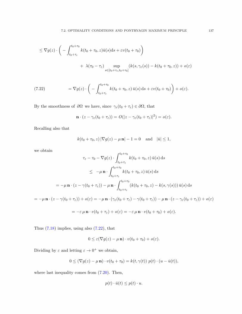
7.2. OPTIMALITY CONDITIONS AND PONTRYAGIN MAXIMUM PRINCIPLE 137
≤ ∇g(z) ·(−∫ t0+τ0
t0+τε
k(t0 + τ0, z)u(s)ds+ εv(t0 + τ0)
)
+ λ(τ0 − τε) sups∈[t0+τε,t0+τ0]
(k(s, γε(s))− k(t0 + τ0, z)) + o(ε)
= ∇g(z) ·(−∫ t0+τ0
t0+τε
k(t0 + τ0, z) u(s) ds+ εv(t0 + τ0)
)+ o(ε).(7.22)
By the smoothness of ∂Ω we have, since γε(t0 + τε) ∈ ∂Ω, that
n · (z − γε(t0 + τε)) = O(|z − γε(t0 + τε)|2) = o(ε).
Recalling also that
k(t0 + τ0, z) |∇g(z)− µn| − 1 = 0 and |u| ≤ 1,
we obtain
τε − τ0 −∇g(z) ·∫ t0+τ0
t0+τε
k(t0 + τ0, z) u(s) ds
≤ −µn ·∫ t0+τ0
t0+τε
k(t0 + τ0, z) u(s) ds
= −µn · (z − γ(t0 + τε))− µn ·∫ t0+τ0
t0+τε
(k(t0 + τ0, z)− k(s, γ(s))) u(s) ds
= −µn · (z − γ(t0 + τε)) + o(ε) = −µn · (γε(t0 + τε)− γ(t0 + τε))− µn · (z − γε(t0 + τε)) + o(ε)
= −ε µn · v(t0 + τε) + o(ε) = −ε µn · v(t0 + τ0) + o(ε).
Thus (7.18) implies, using also (7.22), that
0 ≤ ε(∇g(z)− µn) · v(t0 + τ0) + o(ε).
Dividing by ε and letting ε→ 0+ we obtain,
0 ≤ (∇g(z)− µn) · v(t0 + τ0) = k(t, γ(t)) p(t) · (u− u(t)),
where last inequality comes from (7.20). Then,
p(t) · u(t) ≤ p(t) · u.
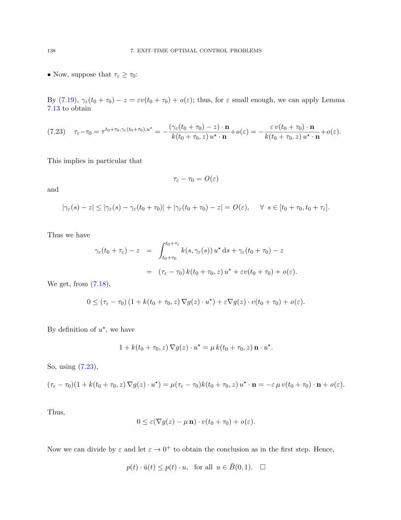
138 7. EXIT-TIME OPTIMAL CONTROL PROBLEMS
• Now, suppose that τε ≥ τ0:
By (7.19), γε(t0 + τ0) − z = εv(t0 + τ0) + o(ε); thus, for ε small enough, we can apply Lemma7.13 to obtain
(7.23) τε−τ0 = τ t0+τ0,γε(t0+τ0),u? = −(γε(t0 + τ0)− z) · nk(t0 + τ0, z)u? · n
+o(ε) = − ε v(t0 + τ0) · nk(t0 + τ0, z)u? · n
+o(ε).
This implies in particular that
τε − τ0 = O(ε)
and
|γε(s)− z| ≤ |γε(s)− γε(t0 + τ0)|+ |γε(t0 + τ0)− z| = O(ε), ∀ s ∈ [t0 + τ0, t0 + τε].
Thus we have
γε(t0 + τε)− z =
∫ t0+τε
t0+τ0
k(s, γε(s))u? ds+ γε(t0 + τ0)− z
= (τε − τ0) k(t0 + τ0, z)u? + εv(t0 + τ0) + o(ε).
We get, from (7.18),
0 ≤ (τε − τ0) (1 + k(t0 + τ0, z)∇g(z) · u?) + ε∇g(z) · v(t0 + τ0) + o(ε).
By definition of u?, we have
1 + k(t0 + τ0, z)∇g(z) · u? = µk(t0 + τ0, z) n · u?.
So, using (7.23),
(τε − τ0)(1 + k(t0 + τ0, z)∇g(z) · u?) = µ(τε − τ0)k(t0 + τ0, z)u? · n = −ε µ v(t0 + τ0) · n + o(ε).
Thus,
0 ≤ ε(∇g(z)− µn) · v(t0 + τ0) + o(ε).
Now we can divide by ε and let ε→ 0+ to obtain the conclusion as in the first step. Hence,
p(t) · u(t) ≤ p(t) · u, for all u ∈ B(0, 1).

7.2. OPTIMALITY CONDITIONS AND PONTRYAGIN MAXIMUM PRINCIPLE 139
Lemma 7.16. Let t0, x0, τ0, γ, u, µ and p be as in the statement of Theorem 7.15. Thenp(t) 6= 0, for every t ∈ [t0, t0 + τ0].
Proof. From (7.16), one obtains that, for every t ∈ [t0, t0 + τ0], |p′(t)| ≤ M |p(t)|. Hence,we get
|p(t)| ≤ |p(s)| eM |t−s|
for every s, t ∈ [t0, t0 + τ0]. Hence, if there exists s ∈ [t0, t0 + τ0] such that p(s) = 0, oneconcludes that p(t) = 0 for every t ∈ [t0, t0 + τ0], which is a contradiction as p(t0 + τ0) =∇g(γ(t0 + τ0))− µn 6= 0, thanks to Lemma 7.14.
Consequently, we get the following
Corollary 7.17. The optimal control u is Lipschitz continuous on [t0, t0 + τ0]. And, theassociated optimal trajectory γ from x0, at time t0, belongs to C1,1([t0, t0 + τ0],Ω), as soon ask is also Lipschitz with respect to t.
Proof. Since p(t) 6= 0 for every t ∈ [t0, t0 + τ0], it follows immediately from the theorem
7.15 that u(t) = − p(t)|p(t)| . Hence,
u ′(t) = −|p(t)| p′(t)− p(t)·p′(t)
|p(t)| p(t)
|p(t)|2
= −∇xk(t, γ(t)) + u(t) · ∇xk(t, γ(t)) u(t).
Hence, |u ′(t)| ≤ C, for some constant C depending only on the Lipschitz constant Lx (w.r.t.x) of the dynamic k.
Suppose that
(7.24) |∇xk(t, x0)−∇xk(t, x1)| ≤ Lxx |x0 − x1|, for all x0, x1 ∈ Ω, t ∈ R+.
Then, this also provides that (γ, u) is the unique solution of the following system
(7.25)
γ′(t) = k(t, γ(t))u(t),
u′(t) = −∇xk(t, γ(t)) + u(t) · ∇xk(t, γ(t))u(t),
γ(t0) = x0,
u|t=t0 = u(t0).
Given an optimal trajectory γ for x0 at time t0, we will say that p is a dual arc associ-ated with γ if it satisfies the properties of Theorem 7.15, that is, if it solves problem (7.16).

140 7. EXIT-TIME OPTIMAL CONTROL PROBLEMS
We now prove that the dual arc p of the theorem 7.15 is included in the superdifferential, withrespect to x, ∇+ϕ of the value function ϕ, where for every t ∈ R+, x ∈ Ω,
∇+ϕ(t, x) :=
p ∈ Rd : lim sup
h→0
ϕ(t, x+ h)− ϕ(t, x)− p · h|h|
≤ 0
.
As a simple consequence of the definitions of D+ϕ and ∇+ϕ, we have the following inclusionΠx(D+ϕ(t, x)) ⊂ ∇+ϕ(t, x). Moreover, the reverse inclusion holds as soon as ϕ is semi-concave(see, for instance, [37, Lemma 3.3.16]).
Proposition 7.18. Under the assumptions of Theorem 7.15, the arc p solution of system(7.16) satisfies
p(t) ∈ ∇+ϕ(t, γ(t)), for all t ∈ [t0, t0 + τ0).
Proof. Fix t ∈ [t0, t0 + τ0). We will show that for all h ∈ Rd with |h| = 1,
ϕ(t, γ(t) + εh) ≤ ϕ(t, γ(t)) + εp(t) · h+ o(ε)
with o(ε) independent of h. Let us define a control strategy by setting
u(s) =
u(s), s ∈ [t, t0 + τ0],
u?, s > t0 + τ0,
where u? = − ∇g(z)−µn|∇g(z)−µn| . Now, let us consider the trajectory γε := γt,γ(t)+εh,u, associated
with u, starting from γ(t) + εh, at time t. Set
τε := τ t,γ(t)+εh,u.
Then we have, for all s ∈ [t, t0 + τ0],
γε(s) = γ(s) + εv(s) + o(ε),
where v is the solution of the linearized problem
v′(s) = u(s)∇xk(s, γ(s)) · v(s), s ∈ [t, t0 + τ0]
v(t) = h,

7.2. OPTIMALITY CONDITIONS AND PONTRYAGIN MAXIMUM PRINCIPLE 141
and o(ε) does not depend on h. We observe that
ϕ(t, γ(t) + εh)− ϕ(t, γ(t)) ≤ τε − (t0 + τ0 − t) + g(γε(t+ τε))− g(z).
The terms on the right-hand side can be estimated as the corresponding terms in formula (7.18).Following the computations of the proof of Theorem 7.15, we obtain
ϕ(t, γ(t) + εh)− ϕ(t, γ(t)) ≤ ε (∇g(z)− µn) · v(t0 + τ0) + o(ε) = ε p(t) · h+ o(ε).
On the other hand, the subdifferential satisfies an analogous property, with a reversed timedirection, as the next result shows. We denote by ∇−ϕ the subdifferential of ϕ with respect tox, i.e., for every (t, x) ∈ R+ × Ω,
∇−ϕ(t, x) :=
p ∈ Rd : lim inf
y→x
ϕ(t, y)− ϕ(t, x)− p · (y − x)
|y − x|≥ 0
.
Proposition 7.19. Let u be an optimal control for (t0, x0) ∈ R+ ×Ω and γ be its associ-ated optimal trajectory. Let p : [t0, t0 + τ0] 7→ Rd be any solution of the adjoint equation
(7.26) p′(t) = −∇xk(t, γ(t))u(t) · p(t), t ∈ [t0, t0 + τ0],
where τ0 = τ t0,x0,u. Suppose that p(t0) ∈ ∇−ϕ(t0, x0), then p(t) ∈ ∇−ϕ(t, γ(t)), for allt ∈ [t0, t0 + τ0).
Proof. Fix t ∈ (t0, t0 + τ0) and let h be any unit vector in Rd. Let v : [t0, t] 7→ Rd be thesolution of
v′(s) = u(s)∇xk(s, γ(s)) · v(s), s ∈ [t0, t]
v(t) = h.
For any ε > 0, let us set γε = γt0,x0+εv(t0),u. Then, it is not difficult to see that
γε(s) = γ(s) + εv(s) + o(ε), s ∈ [t0, t].
By the dynamic programming principle (see Lemma 7.4), the assumption that p(t0) belongs to∇−ϕ(t0, x0) and the fact that p · v is constant, we get

142 7. EXIT-TIME OPTIMAL CONTROL PROBLEMS
ϕ(t, γε(t)) ≥ t0 − t+ ϕ(t0, x0 + εv(t0))
≥ t0 − t+ ϕ(t0, x0) + ε p(t0) · v(t0) + o(ε)
= ϕ(t, γ(t)) + ε p(t) · h+ o(ε).
On the other hand, by the Lipschitz continuity of ϕ (see Proposition 7.10), we have
ϕ(t, γε(t)) = ϕ(t, γ(t) + εv(t)) + o(ε) = ϕ(t, γ(t) + εh) + o(ε),
and so we conclude that
ϕ(t, γ(t) + εh) ≥ ϕ(t, γ(t)) + ε p(t) · h+ o(ε).
By the arbitrariness of h, we deduce that p(t) ∈ ∇−ϕ(t, γ(t)).
7.3. Differentiability of the value function
In this section, we prove that the value function ϕ is differentiable along optimal trajecto-ries, except possibly their endpoints. This kind of results is classical (see [37]) and one can evenobtain more (for instance, in [36] smoothness of the value function in a neighborhood of optimaltrajectories is proven under some suitable conditions). Yet, most of the literature is concernedwith the autonomous case (see in particular [37]), which makes the question non-trivial in thenon-autonomous one.
First of all, let us introduce the following result concerning the semi-concavity of the valuefunction ϕ. The proof is omitted since in Section 7.4 we will prove a much finer result. Beforethat, we assume the following
(7.27) k ∈ C1,1(R+ × Ω),
(7.28) g is semi-concave on ∂Ω.
Proposition 7.20. Under the assumptions (7.2), (7.5), (7.10), (7.27) and (7.28), the valuefunction ϕ is semi-concave on R+ × Ω.
Proof. We refer, for instance, to [37, Theorem 8.2.7].
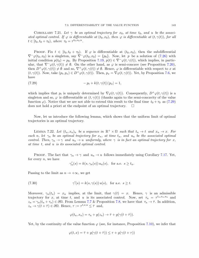
7.3. DIFFERENTIABILITY OF THE VALUE FUNCTION 143
Corollary 7.21. Let γ be an optimal trajectory for x0, at time t0, and u be the associ-ated optimal control. If ϕ is differentiable at (t0, x0), then ϕ is differentiable at (t, γ(t)), for allt ∈ [t0, t0 + τ0), where τ0 = τ t0,x0,u.
Proof. Fix t ∈ [t0, t0 + τ0). If ϕ is differentiable at (t0, x0), then the subdifferential∇−ϕ(t0, x0) is a singleton, say ∇−ϕ(t0, x0) = p0. Now, let p be a solution of (7.26) withinitial condition p(t0) = p0. By Proposition 7.19, p(t) ∈ ∇−ϕ(t, γ(t)), which implies, in partic-ular, that ∇−ϕ(t, γ(t)) 6= ∅. On the other hand, as ϕ is semi-concave (see Proposition 7.20),then D+ϕ(t, γ(t)) 6= ∅ and so, ∇+ϕ(t, γ(t)) 6= ∅. Hence, ϕ is differentiable with respect to x at(t, γ(t)). Now, take (pt, px) ∈ D+ϕ(t, γ(t)). Then, px = ∇ϕ(t, γ(t)). Yet, by Proposition 7.6, wehave
(7.29) − pt + k(t, γ(t)) |px| = 1,
which implies that pt is uniquely determined by ∇ϕ(t, γ(t)). Consequently, D+ϕ(t, γ(t)) is asingleton and so, ϕ is differentiable at (t, γ(t)) (thanks again to the semi-concavity of the valuefunction ϕ). Notice that we are not able to extend this result to the final time t0 + τ0 as (7.29)does not hold a priori at the endpoint of an optimal trajectory.
Now, let us introduce the following lemma, which shows that the uniform limit of optimaltrajectories is an optimal trajectory.
Lemma 7.22. Let (tn, xn)n be a sequence in R+ × Ω such that tn → t and xn → x. Foreach n, let γn be an optimal trajectory for xn, at time tn, and un be the associated optimalcontrol. Then, γn → γ and un → u uniformly, where γ is in fact an optimal trajectory for x,at time t, and u is its associated optimal control.
Proof. The fact that γn → γ and un → u follows immediately using Corollary 7.17. Yet,for every n, we have
γ′n(s) = k(s, γn(s))un(s), for a.e. s ≥ tn.
Passing to the limit as n→ +∞, we get
(7.30) γ′(s) = k(s, γ(s))u(s), for a.e. s ≥ t.
Moreover, γn(tn) = xn implies, at the limit, that γ(t) = x. Hence, γ is an admissibletrajectory for x, at time t, and u is its associated control. Now, set τn = τ tn,xn,un andzn = γn(tn + τn) ∈ ∂Ω. From Lemma 7.7 & Proposition 7.8, we have that τn → τ . In addition,zn → γ(t+ τ) ∈ ∂Ω. Hence, τ := τ t,x,u ≤ τ and,
ϕ(tn, xn) = τn + g(zn)→ τ + g(γ(t+ τ)).
Yet, by the continuity of the value function ϕ (see, for instance, Proposition 7.10), we infer that
ϕ(t, x) = τ + g(γ(t+ τ)) ≤ τ + g(γ(t+ τ))

144 7. EXIT-TIME OPTIMAL CONTROL PROBLEMS
and then, thanks to (7.5), τ = τ .
On the other hand, we have the following result about the uniqueness of optimal control atany interior point of an optimal trajectory.
Proposition 7.23. Let γ be an optimal trajectory from x0 at time t0, and set τ0 = τ t0,x0,u,where u is the associated optimal control. Then, under the assumption (7.24), for every t ∈(t0, t0 + τ0), u is the unique optimal control for γ(t), at time t.
Proof. Fix t ∈ (t0, t0 + τ0) and let v be an optimal control for x := γ(t), at time t. Set
u(s) =
u(s), if s < t,
v(s), if s ≥ t.
Then, it is clear that u is an optimal control for x0, at time t0. Indeed, we have ϕ(t0, x0) ≤τ t0,x0,u + g(γt0,x0,u
τ ) = t − t0 + ϕ(t, x) and so, thanks to Lemma 7.4, the control u is in factoptimal. Hence, by Corollary 7.17, u is continuous, which proves that u(t) = v(t) := q. Thefact that u(s) = v(s), for all s ≥ t, follows from the uniqueness of solution to the system (7.25)with initial conditions γ(t) = x and u(t) = q.
We recall that a vector (h, p) ∈ R+×Rd is called a reachable gradient of ϕ at (t, x) ∈ R+×Ω
if there is a sequence (tk, xk)k such that ϕ is differentiable at (tk, xk) for each k ∈ N, and
limk→∞
(tk, xk) = (t, x), limk→∞
Dϕ(tk, xk) = (h, p).
The set of all reachable gradients of ϕ at (t, x) is denoted by D?ϕ(t, x). It is easily seenthat D?ϕ(t, x) is a compact set: it is closed by definition and it is bounded since ϕ is Lipschitz.From Rademacher’s Theorem it follows that D?ϕ(t, x) 6= ∅ for every (t, x) ∈ R+ × Ω. We havethe following
Proposition 7.24. Let t0, x0, γ, u, τ0 and p be as in the proposition 7.19. Fix t1 ∈ (t0, t0+τ0) and set x1 := γ(t1). Suppose that p(t1) ∈ Πx(D?ϕ(t1, x1)), then p(t) ∈ Πx(D?ϕ(t, γ(t))),for all t ∈ [t1, t0 + τ0].
Proof. If p(t1) ∈ Πx(D?ϕ(t1, x1)), then there is a sequence (t1,n, x1,n) ∈ R+ × Ω suchthat t1,n → t1, x1,n → x1 and ϕ is differentiable at (t1,n, x1,n) with ∇ϕ(t1,n, x1,n) → p(t1).As ϕ is differentiable at (t1,n, x1,n), then, by Corollary 7.21, ϕ is differentiable at (t, γn(t)),for all t ∈ [t1,n, t1,n + τ1,n), where γn is an optimal trajectory for x1,n, at time t1,n, andτ1,n = τ t1,n,x1,n,un ; un being the associated optimal control with γn. Let pn be the solutionof (7.26), associated with γn, with initial condition pn(t1,n) = ∇ϕ(t1,n, x1,n), i.e., pn is the so-lution of the following system
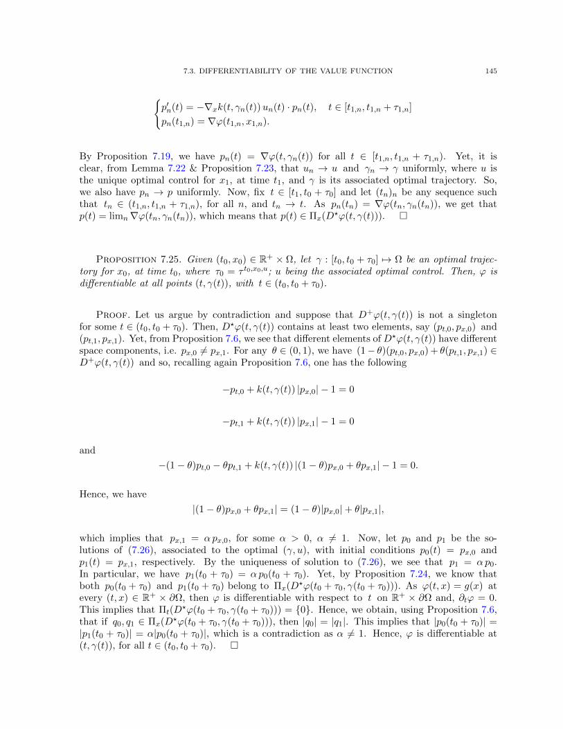
7.3. DIFFERENTIABILITY OF THE VALUE FUNCTION 145
p′n(t) = −∇xk(t, γn(t))un(t) · pn(t), t ∈ [t1,n, t1,n + τ1,n]
pn(t1,n) = ∇ϕ(t1,n, x1,n).
By Proposition 7.19, we have pn(t) = ∇ϕ(t, γn(t)) for all t ∈ [t1,n, t1,n + τ1,n). Yet, it isclear, from Lemma 7.22 & Proposition 7.23, that un → u and γn → γ uniformly, where u isthe unique optimal control for x1, at time t1, and γ is its associated optimal trajectory. So,we also have pn → p uniformly. Now, fix t ∈ [t1, t0 + τ0] and let (tn)n be any sequence suchthat tn ∈ (t1,n, t1,n + τ1,n), for all n, and tn → t. As pn(tn) = ∇ϕ(tn, γn(tn)), we get thatp(t) = limn∇ϕ(tn, γn(tn)), which means that p(t) ∈ Πx(D?ϕ(t, γ(t))).
Proposition 7.25. Given (t0, x0) ∈ R+ × Ω, let γ : [t0, t0 + τ0] 7→ Ω be an optimal trajec-tory for x0, at time t0, where τ0 = τ t0,x0,u; u being the associated optimal control. Then, ϕ isdifferentiable at all points (t, γ(t)), with t ∈ (t0, t0 + τ0).
Proof. Let us argue by contradiction and suppose that D+ϕ(t, γ(t)) is not a singletonfor some t ∈ (t0, t0 + τ0). Then, D?ϕ(t, γ(t)) contains at least two elements, say (pt,0, px,0) and(pt,1, px,1). Yet, from Proposition 7.6, we see that different elements of D?ϕ(t, γ(t)) have differentspace components, i.e. px,0 6= px,1. For any θ ∈ (0, 1), we have (1− θ)(pt,0, px,0) + θ(pt,1, px,1) ∈D+ϕ(t, γ(t)) and so, recalling again Proposition 7.6, one has the following
−pt,0 + k(t, γ(t)) |px,0| − 1 = 0
−pt,1 + k(t, γ(t)) |px,1| − 1 = 0
and
−(1− θ)pt,0 − θpt,1 + k(t, γ(t)) |(1− θ)px,0 + θpx,1| − 1 = 0.
Hence, we have
|(1− θ)px,0 + θpx,1| = (1− θ)|px,0|+ θ|px,1|,
which implies that px,1 = αpx,0, for some α > 0, α 6= 1. Now, let p0 and p1 be the so-lutions of (7.26), associated to the optimal (γ, u), with initial conditions p0(t) = px,0 andp1(t) = px,1, respectively. By the uniqueness of solution to (7.26), we see that p1 = αp0.In particular, we have p1(t0 + τ0) = αp0(t0 + τ0). Yet, by Proposition 7.24, we know thatboth p0(t0 + τ0) and p1(t0 + τ0) belong to Πx(D?ϕ(t0 + τ0, γ(t0 + τ0))). As ϕ(t, x) = g(x) atevery (t, x) ∈ R+ × ∂Ω, then ϕ is differentiable with respect to t on R+ × ∂Ω and, ∂tϕ = 0.This implies that Πt(D
?ϕ(t0 + τ0, γ(t0 + τ0))) = 0. Hence, we obtain, using Proposition 7.6,that if q0, q1 ∈ Πx(D?ϕ(t0 + τ0, γ(t0 + τ0))), then |q0| = |q1|. This implies that |p0(t0 + τ0)| =|p1(t0 + τ0)| = α|p0(t0 + τ0)|, which is a contradiction as α 6= 1. Hence, ϕ is differentiable at(t, γ(t)), for all t ∈ (t0, t0 + τ0).

146 7. EXIT-TIME OPTIMAL CONTROL PROBLEMS
As a consequence of Theorem 7.15, Propositions 7.18 & 7.25, one can characterize an opti-mal control u in terms of the normalized gradient, with respect to x, of the value function ϕ.So, we finish this section by the following
Corollary 7.26. Let (t0, x0) ∈ R+ × Ω and γ = γt0,x0,u be an optimal trajectory for x0,at time t0, where u is the associated optimal control. Then, for all t ∈ (t0, t0 + τ0), whereτ0 := τ t0,x0,u, one has
γ′(t) = −k(t, γ(t))∇xϕ(t, γ(t))
|∇xϕ(t, γ(t))|.
7.4. Sharp semi-concavity
In this section, we investigate the hypotheses under which the value function ϕ of our exit-time optimal control problem is semi-concave with respect to x. Actually, we will refine thesemi-concavity result given in [37] by showing that, instead of assuming (7.27), only a lowerbound on ∂tk (and eventually, we assume that k is C1,1 with respect to x) is sufficient to getthe semi-concavity of ϕ with respect to x. On the other hand, we note that this property isrelated not only to the regularity of the data, but also to the smoothness of the target ∂Ω. Webegin by the following
Proposition 7.27. For every x0, x1 ∈ Ω and t0 ∈ R+, we have, under the assumptions(7.3) & (7.24), the following estimate
∣∣∣∣γt0,x0,u(t) + γt0,x1,u(t) − 2 γt0,x0+x1
2,u(t)
∣∣∣∣ ≤ c|x0 − x1|2, for all t ∈ [t0,∞),
where c := c(t− t0) > 0 and u : [t0,∞) 7→ B(0, 1) is any control strategy.
Proof. First of all, we have
∣∣∣∣γt0,x0,u(t) + γt0,x1,u(t) − 2 γt0,x0+x1
2,u(t)
∣∣∣∣=
∣∣∣∣ ∫ t
t0
k(s, γt0,x0,u(s))u(s) ds +
∫ t
t0
k(s, γt0,x1,u(s))u(s) ds− 2
∫ t
t0
k(s, γt0,x0+x1
2,u(s))u(s) ds
∣∣∣∣.Then, ∣∣∣∣γt0,x0,u(t) + γt0,x1,u(t) − 2 γt0,
x0+x12
,u(t)
∣∣∣∣

7.4. SHARP SEMI-CONCAVITY 147
≤∫ t
t0
∣∣∣∣k(s, γt0,x0,u(s)) + k(s, γt0,x1,u(s))− 2k(s, γt0,x0+x1
2,u(s))
∣∣∣∣ ds
≤∫ t
t0
∣∣∣∣k(s, γt0,x0,u(s)) + k(s, γt0,x1,u(s))− 2k
(s,γt0,x0,u(s) + γt0,x1,u(s)
2
)∣∣∣∣ ds+ 2
∫ t
t0
∣∣∣∣k(s, γt0,x0,u(s) + γt0,x1,u(s)
2
)− k(s, γt0,
x0+x12
,u(s))
∣∣∣∣ds.Yet, by (7.3), one has
2
∫ t
t0
∣∣∣∣k(s, γt0,x0,u(s) + γt0,x1,u(s)
2
)− k(s, γt0,
x0+x12
,u(s))
∣∣∣∣ ds≤ Lx
∫ t
t0
∣∣∣∣γt0,x0,u(s) + γt0,x1,u(s) − 2 γt0,x0+x1
2,u(s)
∣∣∣∣ds.On the other hand, as k is C1,1 with respect to x, we can estimate the first term as fol-lows ∣∣∣∣k(s, γt0,x0,u(s)) + k(s, γt0,x1,u(s))− 2k
(s,γt0,x0,u(s) + γt0,x1,u(s)
2
)∣∣∣∣≤ C|γt0,x0,u(s)− γt0,x1,u(s)|2.
Hence, by Proposition 7.9, we obtain
∫ t
t0
∣∣∣∣k(s, γt0,x0,u(s)) + k(s, γt0,x1,u(s)) − 2k
(s,γt0,x0,u(s) + γt0,x1,u(s)
2
)∣∣∣∣ds ≤ C1 |x1 − x0|2
and then, ∣∣∣∣γt0,x0,u(t) + γt0,x1,u(t)− 2 γt0,x0+x1
2,u(t)
∣∣∣∣≤ C1 |x1 − x0|2 + C
∫ t
t0
∣∣∣∣γt0,x0,u(s) + γt0,x1,u(s)− 2γt0,x0+x1
2,u(s)
∣∣∣∣ ds.

148 7. EXIT-TIME OPTIMAL CONTROL PROBLEMS
We conclude by using the Gronwall’s inequality.
We recall that the property (7.10) (or more generally, a uniform exterior ball condition on Ω)
implies the semi-concavity of the distance function d(·,Rd\Ω) in Ω. Actually, the semi-concavityof this distance function is needed in the proof of the semi-concavity of the value function ϕ. Toprove this semi-concavity result on ϕ, we need to assume that (7.2), (7.3), (7.5), (7.10), (7.11),(7.12), (7.24) and (7.28) are satisfied. In addition, we suppose, instead of (7.27), that we onlyhave a lower bound on the derivative of the dynamic k with respect to t, i.e.,
(7.31) ∂tk ≥ −c.
Then, we have the following
Proposition 7.28. The value function ϕ is semi-concave w.r.t. x, and the semi-concavityconstant depends only on λ, kmin, kmax, κ, Lx, Lxx, M and || [∂tk]− ||∞, where κ is a bound onthe curvatures of ∂Ω, Lx is the Lipschitz constant of k with respect to x, Lxx is the Lipschitzconstant of ∇xk with respect to x and M is a constant such that D2g ≤MI.
Proof. First of all, we consider arbitrary x, x− h, x+ h ∈ Ω and we suppose, for simplic-ity of exposition, that t0 = 0. We want to construct suitable trajectories steering the pointsx, x − h, x + h to the target ∂Ω. More precisely, let us take a control u which is optimalfor x, at time 0, and consider the trajectories γ0,x,u, γ0,x−h,u, γ0,x+h,u starting from the pointsx, x−h, x+h, at time 0, associated with the same control u. We treat separately two differentcases depending on which of these trajectories reaches the target first.
• τ0 := τ0,x,u ≤ minτ0,x−h,u, τ0,x+h,u :
Since u is optimal for x, at time 0, we have by the dynamic programming principle (see Lemma7.4) that
ϕ(0, x− h) + ϕ(0, x+ h) − 2ϕ(0, x) ≤ ϕ(τ0, x−) + ϕ(τ0, x
+) − 2g(γ0,x,uτ ),
where, for simplicity, we set
x+ := γ0,x+h,u(τ0) and x− := γ0,x−h,u(τ0).
Let us now take u+, u− two optimal controls for x+ and x−, at time τ0, respectively. Let
us set for simplicity y± = γτ0,x±,u±
τ to denote the terminal points of the corresponding trajec-tories. Hence, we get
ϕ(τ0, x−) + ϕ(τ0, x
+) − 2g(γ0,x,uτ ) = τ− + g(y−) + τ+ + g(y+)− 2g(γ0,x,u
τ ),

7.4. SHARP SEMI-CONCAVITY 149
where τ± := τ τ0,x±,u± . Yet, by Lemma 7.7 & Proposition 7.8, we have
τ± ≤ c d(x±,Rd\Ω).
As the distance function d(. ,Rd\Ω) is semi-concave, and taking into account that γ0,x,uτ ∈ ∂Ω,
we obtain that
d(x+,Rd\Ω) + d(x−,Rd\Ω)
= d(x+,Rd\Ω) + d(x−,Rd\Ω)− 2d
(x+ + x−
2,Rd\Ω
)+ 2
(d
(x+ + x−
2,Rd\Ω
)−d(γ0,x,u
τ ,Rd\Ω)
)
≤ c|x+ − x−|2 + |x+ + x− − 2γ0,x,uτ | ≤ ch2,
where the last inequality follows from Propositions 7.9 & 7.27. On the other hand, from theassumptions on g, we have
g(y−) + g(y+)− 2 g(γ0,x,uτ ) = g(y−) + g(y+)− 2g
(y+ + y−
2
)+ 2
(g
(y+ + y−
2
)− g(γ0,x,u
τ )
)
(7.32) ≤ c|y+ − y−|2 + λ|y+ + y− − 2 γ0,x,uτ |.
Yet,
|y+ − y−| ≤ |y+ − x+|+ |x+ − x−|+ |x− − y−| ≤ |y+ − x+|+ |x− − y−|+ c|h|.
In addition, we have
|y± − x±| =∣∣∣∣ ∫ τ0+τ±
τ0
k(s, γτ0,x±,u±(s))u±(s) ds
∣∣∣∣ ≤ kmax τ± ≤ ch2,
which implies that|y+ − y−| ≤ c|h|.
For the second term in (7.32), we have

150 7. EXIT-TIME OPTIMAL CONTROL PROBLEMS
|y+ + y− − 2 γ0,x,uτ | ≤ |y+ − x+|+ |x+ + x− − 2 γ0,x,u
τ |+ |x− − y−| ≤ ch2.
Consequently,ϕ(0, x− h) + ϕ(0, x+ h) − 2ϕ(0, x) ≤ ch2.
• τ0 := τ0,x−h,u ≤ minτ0,x,u, τ0,x+h,u:
The analysis of this case will conclude the proof since the remaining case which is τ0,x+h,u ≤minτ0,x,u, τ0,x−h,u is entirely symmetric. By the dynaminc programming principle (see Lemma7.4), we have
ϕ(0, x− h) + ϕ(0, x+ h) − 2ϕ(0, x) ≤ ϕ(τ0, x2)− 2ϕ(τ0, x1) + g(x0),
where, for simplicity, we set
x0 = γ0,x−h,u(τ0), x1 = γ0,x,u(τ0), x2 = γ0,x+h,u(τ0).
We recall that u is also an optimal control starting from x1, at time τ0, with τ1 := τ τ0,x1,u =τ0,x,u − τ0. As x0 ∈ ∂Ω, then, by Lemma 7.7, Propositions 7.8 & 7.9, we get that
τ1 ≤ c d(x1,Rd\Ω) ≤ c|x1 − x0| ≤ c|h|.
We will use the control u?(t) := u( t+τ02 ) for the point x2, at time τ0. We have again twocases which require a separate analysis:
• τ1 <ττ0,x2,u
?
2 :
By the dynamic programming principle (see Lemma 7.4), we have
ϕ(τ0, x2)− 2ϕ(τ0, x1) + g(x0) ≤ ϕ(τ0 + 2τ1, γτ0,x2,u?(τ0 + 2 τ1)) + g(x0) − 2g(γτ0,x1,u
τ ).
Let z1 = γτ0,x1,uτ ∈ ∂Ω and z2 = γτ0,x2,u?(τ0 + 2 τ1). Let v be an optimal control for z2, at
time τ0 + 2τ1, then, by Lemma 7.7 & Proposition 7.8, we have

7.4. SHARP SEMI-CONCAVITY 151
ϕ(τ0 + 2τ1, z2) + g(x0) − 2g(z1)
= τ τ0+2τ1,z2,v + g(γτ0+2τ1,z2,vτ ) + g(x0) − 2g(z1)
≤ c d(z2,Rd\Ω) + g(γτ0+2τ1,z2,vτ ) + g(x0) − 2g(z1)
= c d(z2,Rd\Ω)+2
(g
(x0 + γτ0+2τ1,z2,v
τ
2
)−g(z1)
)+g(γτ0+2τ1,z2,v
τ )+ g(x0)−2g
(x0 + γτ0+2τ1,z2,v
τ
2
).
From (7.5) & (7.28), we infer that
ϕ(τ0+2τ1, z2) + g(x0) − 2g(z1) ≤ c d(z2,Rd\Ω) + c |γτ0+2τ1,z2,vτ −x0|2 + λ |x0+γτ0+2τ1,z2,v
τ −2z1|.
Yet, using Proposition 7.9, we have
|γτ0+2τ1,z2,vτ −x0| ≤ |γτ0+2τ1,z2,v
τ − z2|+ |z2−x2|+ |x2−x0| ≤ |γτ0+2τ1,z2,vτ − z2|+ |z2−x2|+ c|h|.
In addition, by Lemma 7.7 & Proposition 7.8, one has
|γτ0+2τ1,z2,vτ − z2| =
∣∣∣∣ ∫ τ0+2τ1+τv
τ0+2τ1
k
(s, γτ0+2τ1,z2,v(s)
)v(s) ds
∣∣∣∣ ≤ kmax τv ≤ c d(z2,Rd\Ω),
where τv := τ τ0+2τ1,z2,v. In the same way, we have
|z2 − x2| =∣∣∣∣ ∫ τ0+2τ1
τ0
k
(s, γτ0,x2,u?(s)
)u?(s) ds
∣∣∣∣ ≤ 2kmax τ1 ≤ c |h|.
Moreover,
|x0 + γτ0+2τ1,z2,vτ − 2z1| ≤ |x0 + z2 − 2z1| + |γτ0+2τ1,z2,v
τ − z2|
and
|γτ0+2τ1,z2,vτ − z2| ≤ c d(z2,Rd\Ω).
152 7. EXIT-TIME OPTIMAL CONTROL PROBLEMS
Hence, it remains to prove that
d(z2,Rd\Ω) + |x0 + z2 − 2z1| ≤ ch2.
Firstly, let us note that
d(z2,Rd\Ω) ≤ |z2 − 2z1 + x0| + d(2z1 − x0,Rd\Ω).
Yet,
d(2z1 − x0,Rd\Ω) = d(2z1 − x0,Rd\Ω) + d(x0,Rd\Ω) − 2d(z1,Rd\Ω),
as x0, z1 ∈ ∂Ω. Hence, by the semi-concavity of the distance function d(. ,Rd\Ω) and, us-ing Proposition 7.9, we get that
d(2z1 − x0,Rd\Ω) ≤ c|z1 − x0|2 ≤ c(|z1 − x1|+ |x1 − x0|)2 ≤ ch2,
since, we have
|z1 − x1| =∣∣∣∣ ∫ τ0+τ1
τ0
k
(s, γτ0,x1,u(s)
)u(s) ds
∣∣∣∣ ≤ kmax τ1 ≤ c|h|.
On the other hand, let n be the unit outward normal vector at z1 and let w := u(τ0 + τ1) =
− ∇g(z1)−µn|∇g(z1)−µn| be the unit optimal control vector at z1, at time τ0 + τ1 (where µ is the unique
constant so that k(τ0 + τ1, z1)|∇g(z1)− µn| = 1; see Lemma 7.14). Then, there is a unit vectore orthogonal to w such that
2z1 − x0 − z2 = αn + βe.
In fact,
|e · n| = |w · t| =∣∣∣∣ ∇g(z1)− µn
|∇g(z1)− µn|· t∣∣∣∣ =
∣∣∣∣ ∇g(z1)
|∇g(z1)− µn|· t∣∣∣∣ = k(τ0 + τ1, z1)|∇g(z1) · t|,
where t is some unitary tangent vector on the boundary at z1. And, this implies that
(7.33) |e · n| ≤ λkmax < 1.
We have(2z1 − x0 − z2) · n = α+ β e · n
7.4. SHARP SEMI-CONCAVITY 153
and
(2z1 − x0 − z2) · e = α e · n + β.
Then, ((2z1 − x0 − z2) · n(2z1 − x0 − z2) · e
)=
(1 e · n
e · n 1
)(αβ
)
or equivalently, (αβ
)=
(1 e · n
e · n 1
)−1((2z1 − x0 − z2) · n(2z1 − x0 − z2) · e
).
One has
|2z1 − x0 − z2| ≤C
1− (e · n)2
(|(2z1 − x0 − z2) · n| + |(2z1 − x0 − z2) · e|
),
where the denominator can be estimated thanks to (7.33). Firstly, we note that
z2 − 2z1 + x0
= x0 + x2 − 2x1 +
∫ τ0+2τ1
τ0
k(s, γτ0,x2,u?(s))u?(s) ds− 2
∫ τ0+τ1
τ0
k(s, γτ0,x1,u(s))u(s) ds
= x0 + x2 − 2x1 +
∫ τ0+2τ1
τ0
k(s, γτ0,x2,u?(s))u
(s+ τ0
2
)ds− 2
∫ τ0+τ1
τ0
k(s, γτ0,x1,u(s))u(s) ds
= x0 + x2 − 2x1 + 2
∫ τ0+τ1
τ0
(k(2s− τ0, γ
τ0,x2,u?(2s− τ0)) − k(s, γτ0,x1,u(s))
)u(s) ds.
Hence,
(z2 − 2z1 + x0) · e
= (x0 + x2 − 2x1) · e + 2
∫ τ0+τ1
τ0
(k(2s− τ0, γ
τ0,x2,u?(2s− τ0)) − k(s, γτ0,x1,u(s))
)u(s) · e ds.
Yet, from Proposition 7.27, we have

154 7. EXIT-TIME OPTIMAL CONTROL PROBLEMS
|(x0 + x2 − 2x1) · e| ≤ |x0 + x2 − 2x1| ≤ ch2.
To estimate the second term, let us observe, first, that
|u(s)− w| = |u(s)− u(τ0 + τ1)| =∣∣∣∣ ∫ τ0+τ1
su′(t) dt
∣∣∣∣and then, using (7.25), we get, for all s ∈ [τ0, τ0 + τ1], that
|u(s)− w| =
∣∣∣∣ ∫ τ0+τ1
s
(−∇xk(t, γ0,x,u(t)) + (u(t) · ∇xk(t, γ0,x,u(t)))u(t)
)dt
∣∣∣∣≤ c(τ0 + τ1 − s) ≤ c|h|.
This implies that
|u(s) · e| = |(u(s)− w) · e| ≤ c|h|.
Hence,
∣∣∣∣ ∫ τ0+τ1
τ0
(k(2s− τ0, γ
τ0,x2,u?(2s− τ0)) − k(s, γτ0,x1,u(s))
)u(s) · e ds
∣∣∣∣≤ 2 kmax
∫ τ0+τ1
τ0
|u(s) · e|ds ≤ c|h|τ1 ≤ ch2.
Consequently,
|(z2 − 2z1 + x0) · e| ≤ ch2.
On the other hand, we want to show that
|(2z1 − x0 − z2) · n| ≤ ch2.
Let x′0 (resp. z′2) be the projection of x0 (resp. z2) into the tangent space on ∂Ω at z1.

7.4. SHARP SEMI-CONCAVITY 155
Then, we have
(2z1 − x0 − z2) · n = (x′0 − x0) · n + (z′2 − z2) · n.
From (7.10) and the fact that |z1 − x0| ≤ c|h|, it is easy to see that
|x′0 − x0| ≤ ch2.
Moreover, as z2 ∈ Ω and |z2 − z1| ≤ c|h|, then
(z′2 − z2) · n ≥ −ch2.
Consequently,
|(2z1 − x0 − z2) · n| ≤ (2z1 − x0 − z2) · n + ch2.
Yet,(2z1 − x0 − z2) · n
= −(x0 + x2 − 2x1) ·n − 2
∫ τ0+τ1
τ0
(k(2s− τ0, γ
τ0,x2,u?(2s− τ0)) − k(s, γτ0,x1,u(s))
)u(s) ·n ds.
From Proposition 7.27, we get again that
−(x0 + x2 − 2x1) · n ≤ |x0 + x2 − 2x1| ≤ ch2.
For the second term, we have
−∫ τ0+τ1
τ0
(k(2s− τ0, γ
τ0,x2,u?(2s− τ0)) − k(s, γτ0,x1,u(s))
)u(s) · n ds
= −∫ τ0+τ1
τ0
(k(2s− τ0, γ
τ0,x2,u?(2s− τ0)) − k(s, γτ0,x2,u?(2s− τ0))
)u(s) · n ds
−∫ τ0+τ1
τ0
(k(s, γτ0,x2,u?(2s− τ0)) − k(s, γτ0,x1,u(s))
)u(s) · n ds.
156 7. EXIT-TIME OPTIMAL CONTROL PROBLEMS
From (7.3), we have
∣∣∣∣ ∫ τ0+τ1
τ0
(k(s, γτ0,x2,u?(2s− τ0)) − k(s, γτ0,x1,u(s))
)u(s) · n ds
∣∣∣∣≤ C1
∫ τ0+τ1
τ0
|γτ0,x2,u?(2s− τ0) − γτ0,x1,u(s)|ds.
Yet, by Proposition 7.9, one has
∣∣∣∣γτ0,x2,u?(2s− τ0) − γτ0,x1,u(s)
∣∣∣∣=
∣∣∣∣x2 +
∫ 2s−τ0
τ0
k(t, γτ0,x2,u?(t))u?(t) dt − x1 −∫ s
τ0
k(t, γτ0,x1,u(t))u(t) dt
∣∣∣∣≤ |x2 − x1|+
∫ 2s−τ0
τ0
k(t, γτ0,x2,u?(t)) dt +
∫ s
τ0
k(t, γτ0,x1,u(t)) dt
≤ c|h|+ 3 kmax(s− τ0).
Hence, we get ∣∣∣∣ ∫ τ0+τ1
τ0
(k(s, γτ0,x2,u?(2s− τ0)) − k(s, γτ0,x1,u(s))
)u(s) · n ds
∣∣∣∣≤∫ τ0+τ1
τ0
(c|h| + 3 kmax (s− τ0)) ds ≤ ch2.
On the other hand, we have
w · n = − ∇g(z1)− µn
|∇g(z1)− µn|· n = k(τ0 + τ1, z1)(−∇g(z1) · n + µ).
Yet,
|∇g(z1)− µn|2 = µ2 + |∇g(z1)|2 − 2µ∇g(z1) · n =1
k(τ0 + τ1, z1)2.
Then,
2µ(−∇g(z1) · n + µ) =1
k(τ0 + τ1, z1)2− |∇g(z1)|2 + µ2 >
1
kmax2 − λ
2 > 0.

7.4. SHARP SEMI-CONCAVITY 157
Finally, using (7.31), one has
−∫ τ0+τ1
τ0
(k(2s− τ0, γ
τ0,x2,u?(2s− τ0)) − k(s, γτ0,x2,u?(2s− τ0))
)u(s) · n ds
= −∫ τ0+τ1
τ0
(k(2s− τ0, γ
τ0,x2,u?(2s− τ0)) − k(s, γτ0,x2,u?(2s− τ0))
)w · n ds
−∫ τ0+τ1
τ0
(k(2s− τ0, γ
τ0,x2,u?(2s− τ0)) − k(s, γτ0,x2,u?(2s− τ0))
)(u(s)− w) · n ds
≤∫ τ0+τ1
τ0
∫ 2s−τ0
s−kt(t, γτ0,x2,u?(2s− τ0))w · n dtds + ch2 ≤ c(τ2
1 + h2) ≤ ch2.
• τ2 := τ τ0,x2,u? ≤ 2τ1:
Set again
z1 := γτ0,x1,uτ ∈ ∂Ω.
In this case, we have
ϕ(0, x− h) + ϕ(0, x+ h) − 2ϕ(0, x)
≤ ϕ(τ0, x2)− 2ϕ(τ0, x1) + g(x0) ≤ τ2 + g(γτ0,x2,u?
τ )− 2τ1 − 2g(z1) + g(x0)
= τ2 − 2τ1 + 2
(g
(x0 + γτ0,x2,u?
τ
2
)− g(z1)
)+ g(γτ0,x2,u?
τ ) + g(x0) − 2g
(x0 + γτ0,x2,u?
τ
2
).
From (7.28), we get
ϕ(τ0, x2) − 2ϕ(τ0, x1) + g(x0)
≤ τ2 − 2τ1 + c |γτ0,x2,u?
τ − x0|2 + 2
(g
(x0 + γτ0,x2,u?
τ
2
)− g(z1)
).

158 7. EXIT-TIME OPTIMAL CONTROL PROBLEMS
Using Proposition 7.9, we obtain that
|γτ0,x2,u?
τ − x0| ≤ |γτ0,x2,u?
τ − x2|+ |x2 − x0| ≤ |γτ0,x2,u?
τ − x2|+ c|h|.
Yet,
|γτ0,x2,u?
τ − x2| =∣∣∣∣ ∫ τ0+τ2
τ0
k(s, γτ0,x2,u?(s))u?(s) ds
∣∣∣∣ ≤ 2kmax τ1 ≤ c|h|.
On the other hand, we have
g
(x0 + γτ0,x2,u?
τ
2
)− g(z1) ≤ 1
2∇g(z1) · (x0 + γτ0,x2,u?
τ − 2z1) + O(|x0 + γτ0,x2,u?
τ − 2z1|2).
But, it is clear that
|x0 + γτ0,x2,u?
τ − 2z1| ≤ |x0 + x2 − 2x1| + 2
∫ τ0+τ1
τ0
|k(s, γτ0,x1,u(s))u(s)| ds
+
∫ τ0+τ2
τ0
|k(s, γτ0,x2,u?(s))u?(s)|ds,
which implies, using Proposition 7.27, that
|x0 + γτ0,x2,u?
τ − 2z1| ≤ ch2 + 4kmax τ1 ≤ c|h|.
So, it remains to prove that
τ2 − 2τ1 + ∇g(z1) · (x0 + γτ0,x2,u?
τ − 2z1) ≤ ch2.
Let n be the unit outward normal vector at z1. Then, there is a vector e, orthogonal ton, such that
∇g(z1) = αn + βe
with α2 + β2 ≤ λ2. Hence, we get
∇g(z1) · (x0 + γτ0,x2,u?
τ − 2z1) = (αn + βe) · (x0 + γτ0,x2,u?
τ − 2z1)
= αn · (x0 + γτ0,x2,u?
τ − 2z1) + βe · (x0 + γτ0,x2,u?
τ − 2z1).
Recall that
|x0 − z1| + |z1 − γτ0,x2,u?
τ | ≤ c|h|.

7.4. SHARP SEMI-CONCAVITY 159
From (7.10), we infer that
αn · (x0 + γτ0,x2,u?
τ − 2z1) ≤ ch2.
Now, set
z := γτ0,x1,u
(τ0 +
τ2
2
).
Then, one has
τ2 − 2τ1 + βe · (x0 + γτ0,x2,u?
τ − 2z1)
= τ2 − 2τ1 + βe · (x0 + γτ0,x2,u?
τ − 2z) + 2βe · (z − z1).
Let us observe that
|z − z1| =∣∣∣∣ ∫ τ0+τ1
τ0+τ22
k(s, γτ0,x1,u(s))u(s) ds
∣∣∣∣ ≤ kmax
(τ1 −
τ2
2
).
Using kmax |β| ≤ kmax λ < 1, we infer that
τ2 − 2τ1 + βe · (x0 + γτ0,x2,u?
τ − 2z) + 2βe · (z − z1) ≤ βe · (x0 + γτ0,x2,u?
τ − 2z).
So, the aim, now, is to prove that
βe · (x0 + γτ0,x2,u?
τ − 2z) ≤ ch2.
Firstly, let us observe that
x0 + γτ0,x2,u?
τ − 2z
= x0 + x2 − 2x1 − 2
∫ τ0+τ22
τ0
k(s, γτ0,x1,u(s))u(s) ds+
∫ τ0+τ2
τ0
k(s, γτ0,x2,u?(s))u?(s) ds
= x0 + x2 − 2x1 − 2
∫ τ0+τ22
τ0
k(s, γτ0,x1,u(s))u(s) ds+
∫ τ0+τ2
τ0
k(s, γτ0,x2,u?(s))u
(s+ τ0
2
)ds
= x0 + x2 − 2x1 + 2
∫ τ0+τ22
τ0
(k(2s− τ0, γ
τ0,x2,u?(2s− τ0))− k(s, γτ0,x1,u(s))
)u(s) ds

160 7. EXIT-TIME OPTIMAL CONTROL PROBLEMS
= x0 + x2 − 2x1 + 2
∫ τ0+τ22
τ0
(k(2s− τ0, γ
τ0,x2,u?(2s− τ0))− k(s, γτ0,x2,u?(2s− τ0))
)u(s) ds
+ 2
∫ τ0+τ22
τ0
(k(s, γτ0,x2,u?(2s− τ0))− k(s, γτ0,x1,u(s))
)u(s) ds.
Recall that
|x2 + x0 − 2x1| ≤ ch2.
From (7.3), we infer that
∣∣∣∣ ∫ τ0+τ22
τ0
(k(s, γτ0,x2,u?(2s− τ0))− k(s, γτ0,x1,u(s))
)u(s) ds
∣∣∣∣≤ Lx
∫ τ0+τ22
τ0
∣∣∣∣γτ0,x2,u?(2s− τ0)− γτ0,x1,u(s)
∣∣∣∣ ds.Yet, by Proposition 7.9, we have
∣∣∣∣γτ0,x2,u?(2s− τ0)− γτ0,x1,u(s)
∣∣∣∣=
∣∣∣∣x2 +
∫ 2s−τ0
τ0
k(t, γτ0,x2,u?(t))u?(t) dt− x1 −∫ s
τ0
k(t, γτ0,x1,u(t))u(t) dt
∣∣∣∣≤ |x2 − x1|+
∣∣∣∣ ∫ 2s−τ0
τ0
k(t, γτ0,x2,u?(t))u?(t) dt
∣∣∣∣+
∣∣∣∣ ∫ s
τ0
k(t, γτ0,x1,u(t))u(t) dt
∣∣∣∣≤ c|h|+ 3kmax (s− τ0).
Consequently, we get∣∣∣∣ ∫ τ0+τ22
τ0
(k(s, γτ0,x2,u?(2s− τ0))− k(s, γτ0,x1,u(s))
)u(s) ds
∣∣∣∣ ≤ ch2.
On the other hand,

7.4. SHARP SEMI-CONCAVITY 161
∫ τ0+τ22
τ0
(k(2s− τ0, γ
τ0,x2,u?(2s− τ0))− k(s, γτ0,x2,u?(2s− τ0))
)u(s) ds
=
∫ τ0+τ22
τ0
(k(2s− τ0, γ
τ0,x2,u?(2s− τ0))− k(s, γτ0,x2,u?(2s− τ0))
)u(τ0 + τ1) ds
+
∫ τ0+τ22
τ0
(k(2s− τ0, γ
τ0,x2,u?(2s− τ0))− k(s, γτ0,x2,u?(2s− τ0))
)(u(s)− u(τ0 + τ1)) ds
≤∫ τ0+
τ22
τ0
(k(2s− τ0, γ
τ0,x2,u?(2s− τ0))− k(s, γτ0,x2,u?(2s− τ0))
)u(τ0 + τ1) ds + ch2.
We recall that
u(τ0 + τ1) = − ∇g(z1)− µn
|∇g(z1)− µn|,
and so, using (7.31), we get
∫ τ0+τ22
τ0
(k(2s− τ0, γ
τ0,x2,u?(2s− τ0))− k(s, γτ0,x2,u?(2s− τ0))
)u(τ0 + τ1) · βeds
= −k(τ0 + τ1, z1)β2
∫ τ0+τ22
τ0
(k(2s− τ0, γ
τ0,x2,u?(2s− τ0))− k(s, γτ0,x2,u?(2s− τ0))
)ds
= k(τ0 + τ1, z1)β2
∫ τ0+τ22
τ0
∫ 2s−τ0
s−kt(t, γτ0,x2,u?(2s− τ0)) dtds ≤ ch2.
We finish this section by the following remark
Remark 7.29. One can give an example showing that a lower bound on the derivative ofthe dynamic k with respect to t is actually sharp ! To see that, let Ω be the unit ball in Rd. Letκ be a differentiable real function with 0 < κmin ≤ κ ≤ κmax < +∞. Set k(t, x) := κ(t), forevery (t, x) ∈ R+×Ω. For a given x ∈ Ω, the optimal trajectory for x, at time 0, will be given by
γ′(s) = k(s, γ(s)) e(x) = κ(s) e(x),
where e(x) := x/|x|. Let ϕ be the value function associated with this control problem. Hence,

162 7. EXIT-TIME OPTIMAL CONTROL PROBLEMS
we observe easily that ∫ ϕ(0,x)
0κ(s) ds = 1− |x|.
Now, set
G(T ) :=
∫ T
0κ(s) ds, for all T ≥ 0
andH := G−1.
This yields thatϕ(0, x) = H(1− |x|).
Consequently, we have
D2ϕ(0, x) = H ′′(1− |x|) e(x)⊗ e(x)− H ′(1− |x|)|x|
(I − e(x)⊗ e(x)),
where
H ′ =1
κH and H ′′ = − κ
′
κ3H.
This shows that D2ϕ cannot be bounded from above unless κ′ is bounded from below.
CHAPTER 8
Minimal time Mean Field Games
Mean field games (MFG) theory has been introduced simultaneously by Lasry and Lions [79, 80, 81]and by Huang, Malhame and Caines [68, 69] in order to study large population differential games. In thischapter, we are interested in the study of a MFG model motivated by the crowd motion. The understandingof fast exit and evacuation situations in crowd motion research has received a lot of scientific interest inthe last decades (see, for instance, [28]). More precisely, we present a MFG model where agents wantto leave a given bounded domain in minimal time. Each agent is free to move in any direction, but itsmaximal speed is assumed to be bounded in terms of the density of agents in order to take into accountcongestion phenomena. We attack the problem by interpreting equilibria as measures in a space of arcs.In such a relaxed setting, the existence of an equilibrium, in the case of a regular dynamic k, followsby set-valued fixed point arguments (see also [87]). Then, we give the forward-backward system of PDEswhich couples a Hamilton-Jacobi equation (for the value function ϕ of the generic agent) with a continuityequation (for the density ρ of agents). The equilibrium that we will found turns out to be a solution ofthe following system of PDEs
(8.1)
∂tρ−∇ ·
(ρ k ∇ϕ|∇ϕ|
)= 0 in R+ × Ω,
−∂tϕ + k |∇ϕ| = 1 in R+ × Ω,
ρ(0) = ρ0 in Ω, ϕ = g on R+ × ∂Ω,
where k : P(Ω) × Ω 7→ R+ is the dynamic and g : ∂Ω 7→ R+ is a given boundary cost. We note
that it is much simpler here to use the Lagrangean approach, instead of using the Schauder fixed point
Theorem applied to the Eulerian formulation (i.e. doing a fixed point on the PDE system, as in [38]),
to prove existence of a solution for (8.1); this is due to the fact that the velocity v = −k ∇ϕ|∇ϕ| is a priori
non-regular. On the other hand, we are able to give Lp estimates on the density of agents ρt, at each
time t, as soon as the initial density ρ0 belongs to Lp. Moreover, thanks to these Lp estimates, we extend
the result of existence of an equilibrium to a case where the dynamic k is non-regular.
This chapter will be a part of a joint paper with G. Mazanti, in preparation, [57].
8.1. Existence of equilibria in the regular case
Let Ω be a compact domain in Rd. We denote by P(Ω) the family of all Borel probabilitymeasures on Ω. Let k : P(Ω) × Ω 7→ R+ be a continuous function. We consider the followingoptimal-exit problem: agents evolve in Ω, their distribution at time t being given by the prob-ability measure ρt. The goal of each agent is to leave the boundary ∂Ω in minimal time (i.e.,paying a minimal cost that is assumed to be given by the time to reach a possible exit-pointplus a boundary cost g at this point, where g : ∂Ω 7→ R+ is a given continuous function), butwe assume the speed of an agent in a position x at time t to be bounded by k(ρt, x). This
163
164 8. MINIMAL TIME MEAN FIELD GAMES
means that, for a given agent, its trajectory γ depends on the distribution of all agents ρt, sincethe speed of γ should not exceed k(ρt, x). On the other hand, the distribution of the agentsρt itself depends on how agents choose their trajectories γ. Thus, we are interested here in theequilibrium situations, i.e., in situations where, starting from a time evolution of the density ofagents ρ : R+ → P(Ω), the trajectories γ chosen by agents induce an evolution of the initialdistribution of agents ρ0 that is precisely given by ρ. For every point x ∈ Ω, we consider thefollowing problem
(8.2) inf
τγ + g(γτ ) : γ ∈ Γ[ρ, x]
,
where
Γ[ρ, x] :=
γ ∈ Γ, γ(0) = x, |γ′(s)| ≤ k(ρs, γ(s)) for a.e. s ∈ (0, τγ) and γ′(s) = 0 ∀ s > τγ
,
τγ := infs ≥ 0 : γ(s) ∈ ∂Ω,
γτ := γ(τγ) ∈ ∂Ω,
and Γ is the space of all continuous curves from R+ to Ω, equipped with the topology of uni-form convergence on compact sets, with respect to which Γ is a Polish space (see, for instance,[17]).
Remark 8.1. If γ belongs to Γ[ρ, x], then there is a control u : R+ 7→ B(0, 1) such that
(8.3)
γ′(t) = k(ρt, γ(t))u(t), for a.e. t,
γ(0) = x.
Moreover, (8.3) can be seen as a control system (see Chapter 7) where the dynamic is given
by k(t, x) = k(ρt, x) for every (t, x) ∈ R+×Ω. This point of view allows one to formulate (8.2)as an optimal control problem.
Let us state some assumptions on the data. It is reasonable to suppose that the dynamic kis bounded from above, since if this is not the case, the speed of an agent would be +∞, whichis not natural at all. For simplicity, and in order to affirm that there is at least one admissi-ble trajectory γ, starting from a point x, that reaches the boundary in finite time, we want tosuppose also that the dynamic k is bounded from below. Thus, we assume (as in Chaptre 7) that
0 < kmin := inf k ≤ kmax := sup k < +∞.
Moreover, we suppose, as in the previous chapter, that the cost g is λ-Lipschitz with λ < 1/kmax.In this way, from Proposition 7.2, we infer that (8.2) reaches a minimum.
Following almost the same ideas proposed in [11, 34], we define a “relaxed” notion of MFGequilibria, for which we give existence result. Such a formulation consists of replacing curves
8.1. EXISTENCE OF EQUILIBRIA IN THE REGULAR CASE 165
of probability measures on Ω with measures on arcs in Ω. For any t ∈ R+, we denote byet : Γ 7→ Ω the evaluation map defined by
et(γ) = γ(t), for all γ ∈ Γ.
Let P(Γ) be the set of all probability measures on Γ. For any η ∈ P(Γ), we define the curve ρη
of probability measures on Ω as follows
ρη(t) = (et)#η, for all t ∈ R+.
Since et : Γ 7→ Ω is continuous, we observe that if ηn, η ∈ P(Γ), n ≥ 1, is such that ηn η,then ρηn(t) ρη(t) for all t ∈ R+. For any fixed ρ0 ∈ P(Ω), we denote by Pρ0(Γ) the set ofall Borel probability measures η on Γ such that (e0)#η = ρ0.
Remark 8.2. We note that Pρ0(Γ) is nonempty. Indeed, let j : Ω 7→ Γ be the continuousmap defined by
j(x)(t) = x, for all t ∈ R+.
Then,η := j#ρ0 belongs to Pρ0(Γ).
For all x ∈ Ω and η ∈ Pρ0(Γ), we define
Γ′[ρη, x] :=
γ ∈ Γ[ρη, x] : J(γ) = min
Γ[ρη ,x]J
,
whereJ(γ) := τγ + g(γτ ).
Definition 8.3. Let ρ0 ∈ P(Ω). We say that η ∈ Pρ0(Γ) is a MFG equilibrium for ρ0 if
spt(η) ⊆⋃x∈Ω
Γ′[ρη, x].
In fact, we are able to prove that⋃x Γ′[ρη, x] is closed and so, η ∈ Pρ0(Γ) is a MFG equilibrium
for ρ0 if for η−a.e. γ ∈ Γ, we have
J(γ) ≤ J(γ), for all γ ∈ Γ[ρη, γ(0)].
We recall that k is continuous on P(Ω)× Ω. Moreover, we assume that
|k(µ, x0)− k(µ, x1)| ≤ C|x0 − x1|, for all x0, x1 ∈ Ω, µ ∈ P(Ω).

166 8. MINIMAL TIME MEAN FIELD GAMES
Then, we have the following main result.
Theorem 8.4. Under these assumptions, there exists a MFG equilibrium for ρ0.
Before proving this theorem, we introduce the following
Lemma 8.5. Let ηn, η ∈ Pρ0(Γ) be such that ηn η. Let xn ∈ Ω be such that xn → x andlet γn ∈ Γ′[ρηn , xn] be such that γn → γ. Then γ ∈ Γ′[ρη, x]. Consequently, (η, x) 7→ Γ′[ρη, x]has a closed graph.
Proof. We set, for simplicity, τn := τγn and zn := γn(τn). Using Lemma 7.7 & Proposition7.8, (τn)n is bounded and, up to a subsequence, τn converges to some τ . On the other hand,we see easily that γ ∈ Lip(R+,Ω) with |γ′| ≤ kmax. In addition, we have
|γ′n(t)| ≤ k(ρηn(t), γn(t)), for a.e. t ∈ (0, τn).
Letting n→ +∞, we get that
|γ′(t)| ≤ k(ρη(t), γ(t)), for a.e. t ∈ (0, τ).
In the same way, one can prove that γ′(t) = 0 for all t > τ . Moreover, we have
zn → γ(τ),
which implies that γ(τ) ∈ ∂Ω and τ := τγ ≤ τ . Define the trajectory γ ∈ Γ[ρη, x] as follows
γ(t) =
γ(t), if t ≤ τ,γ(τ), if t > τ.
Suppose that γ /∈ Γ′[ρη, x]. Then, there is a trajectory γ ∈ Γ′[ρη, x] such that J(γ) < J(γ),which means that we have
τγ + g(γτ ) < τ + g(γτ ).
For each n, let γn be a geodesic (which is a segment unless x ∈ ∂Ω) between xn and x suchthat |γn′| = 1 and let φn be a function satisfying
φ′n(t) = k(ρηn (t),γ(φn(t)))k(ρη(φn(t)),γ(φn(t))) ,
φn(k−1mind(xn, x)) = 0.
Define
γn(t) =
γn(kmint) for all t ∈ [0, k−1
mind(xn, x)],
γ(φn(t)) else.
8.1. EXISTENCE OF EQUILIBRIA IN THE REGULAR CASE 167
It is clear that γn ∈ Γ[ρηn , xn]. Moreover, we have
(8.4) J(γn) = φ−1n (τ γ) + g(γτ ).
On the other hand, we see that there exists a limit φ such that, up to a subsequence, φn → φuniformly on compact sets of R+. In addition, it is easy to check that for all t ∈ R+,∫ φn(t)
0k(ρη(s), γ(s)) ds =
∫ t
k−1mind(xn,x)
k(ρηn(s), γ(φn(s))) ds.
So, letting n→ +∞, we get∫ φ(t)
0k(ρη(s), γ(s)) ds =
∫ t
0k(ρη(s), γ(φ(s))) ds.
Set
G(θ) =
∫ θ
0k(ρη(s), γ(s)) ds, ∀ θ ∈ R+.
One has
|φ(t)− t| =
∣∣∣∣G−1
(∫ t
0k(ρη(s), γ(φ(s))) ds
)−G−1
(∫ t
0k(ρη(s), γ(s)) ds
)∣∣∣∣≤ C
∫ t
0|k(ρη(s), γ(φ(s))) − k(ρη(s), γ(s))| ds
≤ C
∫ t
0|φ(s) − s| ds.
By using Gronwall’s Lemma, we get that
φ(t) = t, for all t ∈ R+.
Passing to the limit in (8.4), we get
(8.5) limnJ(γn) = lim
nφ−1n (τ γ) + g(γτ ) = J(γ) < J(γ).
As g is λ−Lip with λ < 1/kmax, then
J(γ) ≤ τ + g(γ(τ)).
Yet,
limnJ(γn) = lim
nτn + g(zn) = τ + g(γ(τ)).

168 8. MINIMAL TIME MEAN FIELD GAMES
Using (8.5), we infer that, for n large enough,
J(γn) < J(γn),
which is a contradiction, as γn ∈ Γ[ρηn , xn] and γn ∈ Γ′[ρηn , xn]. In the same way, we see thatτ = τ . Then, γ ∈ Γ′[ρη, x].
Now, we want to prove Theorem 8.4 using a fixed point argument. We introduce the set-valuedmap E : Pρ0(Γ) ⇒ Pρ0(Γ) by defining, for any η ∈ Pρ0(Γ),
E(η) =
η ∈ Pρ0(Γ) : spt(η) ⊆
⋃x∈Ω
Γ′[ρη, x]
.
Then, it is immediate to realize that η ∈ Pρ0(Γ) is a MFG equilibrium for ρ0 if and only ifη ∈ E(η). We will therefore show that the set-valued map E has a fixed point. For this pur-pose, we will apply Kakutani’s Theorem [72]. The following lemmas are intended to check thatthe assumptions of such a theorem are satisfied by E.
Lemma 8.6. For any η ∈ Pρ0(Γ), E(η) is a nonempty convex set.
Proof. First, we note that E(η) is a nonempty set. Indeed, by Lemma 8.5 and [5, 40], wehave that x 7→ Γ′[ρη, x] has a Borel measurable selection γγγη : x 7→ γηx ∈ Γ′[ρη, x]. Thus, themeasure η, defined by η := γγγη#ρ0 belongs to E(η). On the other hand, it is clear that E(η) is aconvex set.
Lemma 8.7. The multimap E : Pρ0(Γ) ⇒ Pρ0(Γ) has a closed graph.
Proof. Let ηn, η ∈ Pρ0(Γ) be such that ηn η. Let ηn ∈ E(ηn) be such that ηn η.Since ηn η, we have that η ∈ Pρ0(Γ). For k ∈ N?, let Vk := γ ∈ Γ : d(γ,∪xΓ′[ρη, x]) ≤ 1
k.By Lemma 8.5, we see that there exists a neighborhood W of η such that
⋃x Γ′[ρη, x] ⊂ Vk,
for every η ∈ W . Then, for n large enough,⋃x Γ′[ρηn , x] ⊂ Vk. Since ηn(
⋃x Γ′[ρηn , x]) = 1,
one obtains that ηn(Vk) = 1, for large n. Yet, ηn η and Vk is closed, it follows thatη(Vk) ≥ lim supn ηn(Vk) = 1 and thus, η(Vk) = 1. As this holds for every k ∈ N?, then oneconcludes that η(
⋃x Γ′[ρη, x]) = 1. Hence η ∈ E(η), which proves that the graph of E is
closed.
Let us denote by Γkmax the set of trajectories γ ∈ Γ such that γ is kmax−Lipschitz, i.e.,
Γkmax = γ ∈ Γ : |γ′| ≤ kmax.

8.1. EXISTENCE OF EQUILIBRIA IN THE REGULAR CASE 169
By the definition of E(η), we deduce that
E(η) ⊂ Pρ0(Γkmax), for all η ∈ Pρ0(Γ).
Remark 8.8. Notice that Pρ0(Γkmax) is a compact convex subset of Pρ0(Γ). The convexityof Pρ0(Γkmax) follows immediately. As for compactness, let (ηk)k ⊂ Pρ0(Γkmax). Since Γkmax
is a compact set, (ηk)k is tight. So, by Prokhorov’s Theorem, one finds a subsequence whichconverges weakly to some probability measure η ∈ Pρ0(Γkmax).
So, we will restrict our domain of interest to Pρ0(Γkmax). Hereafter, we denote by E the re-striction E | Pρ0 (Γkmax ).
Conclusion:
By Remark 8.2 and Remark 8.8, Pρ0(Γkmax) is a nonempty compact convex set. Moreover,by Lemma 8.6, E(η) is a nonempty convex set for any η ∈ Pρ0(Γkmax) and, by Lemma 8.7,the set-valued map E has a closed graph. Then, the assumptions of Kakutani’s Theorem aresatisfied and so, there exists η ∈ Pρ0(Γkmax) such that η ∈ E(η).
We finish this section by characterizing the density ρt := ρη(t) = (et)#η, for some equilibriumη, as a solution of a continuity equation of the form ∂tρ+∇x · (ρ v) = 0 for a particular velocityfield v. Let ϕ be the value function (see Chapter 7), associated to the control problem with
dynamic k(t, x) = k(ρt, x), for all (t, x) ∈ R+ × Ω. Then, under the assumption that k ∈ C1,1,we have the following:
Proposition 8.9. Let η ∈ Pρ0(Γ) be an equilibrium for ρ0. Then ρ : t 7→ ρη(t) is a solutionof
(8.6) ∂tρ(t, x)−∇ ·(ρ(t, x) k(ρt, x)
∇ϕ(t, x)
|∇ϕ(t, x)|
)= 0 in (0,∞)×
Ω.
Proof. Let φ ∈ C∞c ((0,∞) ×Ω). Then, recalling Proposition 7.25 & Corollary 7.26, we
have
−∫ +∞
0
∫Ω∂tφ(t, x) dρt(x) dt +
∫ +∞
0
∫Ωk(ρt, x)∇xφ(t, x) · ∇ϕ(t, x)
|∇ϕ(t, x)|dρt(x) dt
= −∫ +∞
0
∫Γ∂tφ(t, γ(t)) dη(γ) dt +
∫ +∞
0
∫Γk(ρt, γ(t))∇xφ(t, γ(t)) · ∇ϕ(t, γ(t))
|∇ϕ(t, γ(t))|dη(γ) dt
= −∫ +∞
0
∫Γ∂tφ(t, γ(t)) dη(γ) dt −
∫ +∞
0
∫Γ∇xφ(t, γ(t)) · γ′(t) dη(γ) dt
170 8. MINIMAL TIME MEAN FIELD GAMES
= −∫
Γ
∫ +∞
0
d
dt(φ(t, γ(t))) dt dη(γ) = 0.
Let η ∈ Pρ0(Γ) be an equilibrium, ρ = ρη, i.e. ρt = ρη(t) = (et)#η for every t ∈ R+, and ϕbe the associated value function. Then, by Propositions 7.5 & 8.9, (ρ, ϕ) solves the followingsystem
∂tρ(t, x)−∇ ·(ρ(t, x) k(ρt, x)
∇xϕ(t, x)
|∇xϕ(t, x)|
)= 0, (t, x) ∈ (0,∞)× Ω,
− ∂tϕ(t, x) + k(ρt, x) |∇xϕ(t, x)| = 1, (t, x) ∈ R+ × Ω,
ϕ(t, x) = g(x), (t, x) ∈ R+ × ∂Ω,
ρ(0, x) = ρ0(x), x ∈ Ω.
8.2. Lp estimates
In this section, we will be interested in the case where the dynamic k is given by the following
k(ρ, x) = c
(∫Ωχ(x− y)ψ(y) dρ(y)
), for all (ρ, x) ∈ P(Ω)× Ω,
where χ is a non-negative C1,1 function on Rd, ψ is a cut-off function on Ω and c is a positiveC1,1 decreasing function on R+. The meaning of this dynamic k is that each agent evaluatesan average density of agents around him through the integral term, the convolution kernel χand the cut-off function ψ (which allows us to not take into account agents who have alreadyleft the domain, and who remain on ∂Ω), and its maximum speed depends on this evaluation ofthe density across c.
More precisely, we take ψ(x) := α(d(x, ∂Ω)), for every x ∈ Ω, where α is a non-negative C1,1
increasing function such that α = 0 on [0, ε/2] and α = 1 on [ε,+∞), where ε > 0 is smallenough. As we have
∫Ω χ(x − y)ψ(y) dρ(y) ≤ M , for all (ρ, x) ∈ P(Ω) × Ω (we note that the
constant M is independent of ε), then
(8.7) 0 < cmin := min[0,M ]
c ≤ k ≤ cmax := max[0,M ]
c < +∞.
In addition, it is clear that k is (uniformly in ε) C1,1 with respect to the variable x and iscontinuous in ρ. From Theorem 8.4, we infer that, for any ρ0 ∈ P(Ω), there exists an equilib-rium η for ρ0, associated to our MFG model with the dynamic k. On the other hand, we havek((et)#η, x) = c(
∫Γ χ(x − γ(t))ψ(γ(t)) dη(γ)) and so, k is Lipschitz (but, not uniformly in ε)
with respect to t. Yet, we want to show that ∂tk ≥ −C, for some constant C independent of ε.In fact, one has
∂tk = c′(·)(−∫
Γ∇χ(x− γ(t)) · γ′(t)ψ(γ(t)) dη(γ) +
∫Γχ(x− γ(t))∇ψ(γ(t)) · γ′(t) dη(γ)
).

8.2. Lp ESTIMATES 171
We recall that η is concentrated on the optimal trajectories for the control problem associatedwith the dynamic k. Fix such a trajectory γ (we recall from Corollary 7.17 that γ is C1,1) andlet u be its associated optimal control. We have
∇ψ(γ(t)) · u(t) = α′(d(γ(t), ∂Ω))∇d(γ(t), ∂Ω) · u(t).
From Theorem 7.15, we have
u(τγ) = − ∇g(γ(τγ))− µn
|∇g(γ(τγ))− µn|
and so,
∇d(γ(τγ), ∂Ω) · u(τγ) = n · ∇g(γ(τγ))− µn
|∇g(γ(τγ))− µn|= k(τγ , γ(τγ))[−µ+∇g(γ(τγ)) · n].
Using Lemma 7.14, we infer that
∇d(γ(τγ), ∂Ω) · u(τγ) =k(τγ , γ(τγ))
2µ
(− µ2 + |∇g(γ(τγ))|2 − 1
k(τγ , γ(τγ))2
).
As |∇g| ≤ λ < 1cmax
and µ ≥ 1k − |∇g| ≥
1cmax− λ, we get
∇d(γ(τγ), ∂Ω) · u(τγ) ≤ −C,
for some constant C := C(λ, cmin, cmax) > 0. On the other hand, we have
d
dt[∇d(γ(t), ∂Ω) · u(t)] = k((et)#η, γ(t))D2d(γ(t), ∂Ω)u(t) · u(t) +∇d(γ(t), ∂Ω) · u′(t).
Recalling (7.25), we obtain that, for γ(t) close to ∂Ω,
d
dt[∇d(γ(t), ∂Ω) · u(t)] ≥ −M,
where M is a constant independent of ε. Hence, we get
∇d(γ(τγ), ∂Ω) · u(τγ)−∇d(γ(t), ∂Ω) · u(t) ≥ −M(τγ − t)
172 8. MINIMAL TIME MEAN FIELD GAMES
and so, using Lemma 7.7 & Proposition 7.8, we infer that
−C +Md(γ(t), ∂Ω) ≥ −C +M(τγ − t) ≥ ∇d(γ(t), ∂Ω) · u(t).
Consequently, there is some finite constant C, independent of ε, such that ∂tk ≥ −C. Thanksto Proposition 7.28, the value function ϕ, associated to the control problem with the dynamick, is (uniformly in ε) semi-concave with respect to x.
On the other hand, we see easily that k is C1,1 in R+ × Ω. Now, if η is a MFG equilib-rium for ρ0 and ρt = 1
Ω· (et)#η for all t ∈ R+, then, by Corollary 7.26, we get that the pair
(ρt, ϕ) solves the following continuity equation
∂tρt −∇ ·(ρt k(ρt, ·)
∇ϕ|∇ϕ|
)= 0.
So, thanks to the semi-concavity with respect to x of the value function ϕ, we are able tofind Lp estimates on the density of agents ρt, at time t. More precisely, we have the following
Proposition 8.10. For every t ∈ R+, ρt ∈ Lp(Ω) as soon as ρ0 belongs to Lp(Ω). More-over, we have the following estimate
||ρt||Lp(Ω) ≤ C||ρ0||Lp(Ω),
for some constant C depending only on the semi-concavity constant (w.r.t. x) of the value func-tion ϕ.
Proof. First of all, let us define the vector field v as follows: for all t ∈ R+, we set
vt(x) :=
−k(ρt, x) ∇ϕ(t,x)
|∇ϕ(t,x)| , if x ∈Ω,
0, else.
Thanks to the fact that the value function ϕ is semi-concave with respect to x (see Propo-sition 7.28), |∇ϕ| is bounded from below (see Corollary 7.12), and k is Lipschitz with respectto x, we have ∇ · vt ≥ −C. This bound implies a lower bound on the Jacobian determinant Jof the flux associated to
X ′(t, x) = vt(X(t, x)),
X(0, x) = x.

8.2. Lp ESTIMATES 173
Indeed, if X ∈Ω, we have
d
dt∇X = ∇vt(X)∇X.
Setting Jt := det(∇X(t, ·)), one has
d
dtJt(x) = ∇ · vt(X(t, x)) Jt(x)
≥ −C Jt(x).
Hence,
log(Jt(x))− log(J0(x)) ≥ −Ct.
Yet, J0 = 1. So, we get
Jt ≥ e−Ct, for all t ∈ R+.
As η is an equilibrium and ρt = 1 Ω· (et)#η, then, by Corollary 7.26 and the definition of
the flow X, we infer that
ρt = 1 Ω·X(t, ·)#ρ0,
or equivalently,
ρt = 1Xt(Ω)∩
Ω· (ρ0/Jt) (Xt)
−1, for all t ∈ R+.
Hence,
||ρt||pLp(Ω) =
∫Xt(Ω)∩
Ω
ρ0((Xt)−1(y))p
Jt((Xt)−1(y))pdy =
∫Ω
ρ0(x)p
Jt(x)p−11X−1t (
Ω)
(x) dx ≤ eC(p−1)t ||ρ0||pLp(Ω).
Consequently,
||ρt||Lp(Ω) ≤ eC(1− 1
p)t ||ρ0||Lp(Ω).
These estimates are proved, first, for smooth velocity field v and then, by approximation fornon-smooth v with [∇ · vt]− ≤ C (see [2]), using the a.e. uniqueness of the flow of the non-smooth vector fields v, which comes from the uniqueness of the optimal trajectories in optimalcontrol (see Proposition 7.23).

174 8. MINIMAL TIME MEAN FIELD GAMES
8.3. Existence of equilibria for less regular model
Thanks to the previous Lp estimates on ρt, we are able to prove existence of an equilibrium ηfor ρ0 in the case where the dynamic k is given by
k(ρ, x) = c
(∫Ωχ(x− y)1
Ω(y) dρ(y)
), for all (ρ, x) ∈ P(Ω)× Ω.
Notice that the lack of continuity of the dynamic k with respect to ρ prevents us from us-ing the result of Section 8.1. So, the idea will be to consider a sequence of cut-off functions(ψε)ε>0 constructed as in Section 8.2 and converging to 1
Ωin Lq, for all q < +∞, when ε→ 0,
and to replace the dynamic k with kε, where kε is defined as follows
kε(ρ, x) = c
(∫Ωχ(x− y)ψε(y) dρ(y)
), for all (ρ, x) ∈ P(Ω)× Ω.
In this way, if ηε is a MFG equilibrium for ρ0, associated to the control problem with thedynamic kε, then we prove that ηε η where η is, in fact, a MFG equilibrium for ρ0, asso-ciated to the control problem with the dynamic k. First of all, set ρεt = 1
Ω· (et)#η
ε, for all
t ∈ R+, ε > 0. From Section 8.2, we recall that kε is uniformly bounded in ε. Moreover, kε isuniformly C1,1 with respect to x and, we have
∂tkε ≥ −C,
where the constant C is, in fact, independent of ε. As a consequence of that, the value functionϕε, associated to the control problem with the dynamic kε, will be (uniformly in ε) semi-concavewith respect to x (see Proposition 7.28). Then, the proposition 8.10 implies the following uniformestimates
||ρεt ||Lp ≤ C||ρ0||Lp , for all t ∈ R+, ε > 0.
As ηε ∈ P(Γ) and spt(ηε) ⊂ Γcmax (we recall that Γcmax is the set of all cmax-Lip curvesin Γ, which is by the way a compact subset of it), then, up to a subsequence, ηε η. Setρt := 1
Ω· (et)#η, for every t ∈ R+. Hence, we have ρεt ρt in Lp. In addition, ψε → 1
Ωin
Lq, for all q < +∞. Using these facts, we get, for every (t, x) ∈ R+ × Ω, that
kε((et)#ηε, x) = c
(∫Ωχ(x − y)ψε(y)ρεt (y) dy
)→ c
(∫Ωχ(x − y)ρt(y) dy
)= k((et)#η, x).
Moreover, for any x ∈ Ω, the function t 7→ k((et)#η, x) is continuous on R+. Indeed, if tn → t,

8.3. EXISTENCE OF EQUILIBRIA FOR LESS REGULAR MODEL 175
then ρtn ρt in Lp and so, we have
k((etn)#η, x) = c
(∫Ωχ(x − y)ρtn(y) dy
)→ c
(∫Ωχ(x − y)ρt(y) dy
)= k((et)#η, x).
Let us denote by ϕ the value function associated to the control problem with the dynamick. Then, we prove that ϕε → ϕ uniformly, which will be sufficient to infer that η is a MFGequilibrium for ρ0, associated to the control problem with the dynamic k. In fact, we have thefollowing
Proposition 8.11. Let kε, k : P(Ω) × Ω 7→ R+ be such that, for every ε > 0, kε is con-tinuous on P(Ω) × Ω and is Lipschitz with respect to the second variable. Let ηε be a MFGequilibrium, associated to the control problem with dynamic kε, and let η be the limit of ηε inP(Γ). In addition, assume the following:
• There exist two constants cmin and cmax such that 0 < cmin ≤ kε ≤ cmax < +∞.• There exists a constant M independent of ε such that |∇xkε| ≤M.• For a.e. t ∈ R+, we have kε((et)#η
ε, ·)→ k((et)#η, ·) when ε→ 0.• t 7→ k((et)#η, ·) is continuous on R+.
If ϕε (resp. ϕ) is the value function associated to the control problem with dynamic kε (resp.k), then ϕε → ϕ uniformly in R+ × Ω.
Proof. First of all, let us see that ϕε converges uniformly to some function ϕ on R+ ×Ω.Indeed, from Lemma 7.7 & Proposition 7.8, the sequence (ϕε)ε is equibounded. Moreover, byProposition 7.10, the value function ϕε is Lipschitz in R+ × Ω with a Lipschitz constant de-pending only on the Lipschitz constant of the dynamic kε with respect to x, which is by theway uniform in ε. Fix (t, x) ∈ R+×Ω. For every ε > 0, let γε be an optimal trajectory for x, attime t, in the control problem with dynamic kε. It is easy to observe that γε → γ uniformly, forsome γ ∈ Γcmax . Yet, this γ is, in fact, an admissible trajectory for x, at time t, in the controlproblem with dynamic k. Indeed, for a.e. s ∈ (t,∞), we have
|γ′ε(s)| ≤ kε((es)#ηε, γε(s)).
So, letting ε→ 0, we get
|γ′(s)| ≤ k((es)#η, γ(s)), for a.e. s.
Let uε be the optimal control associated with γε and, set
τε := τ t,x,uε and zε := γε(t+ τε) ∈ ∂Ω.
It is clear that τε → τ and zε → z ∈ ∂Ω. In particular, we have z = γ(t + τ) and τγ ≤ τ .Consequently, ϕ(t, x) ≤ τ + g(z) = lim
ε→0ϕε(t, x) = ϕ(t, x).

176 8. MINIMAL TIME MEAN FIELD GAMES
On the other hand, let γ be an optimal trajectory for x, at time t, in the control problemwith dynamic k, and u be the associated optimal control with γ. Let φε be a solution of thefollowing
(8.8)
φ′ε(s) =
kε((es)#ηε,γ(φε(s)))
k((eφε(s))#η,γ(φε(s))),
φε(t) = t.
Setγε(s) = γ(φε(s)), for all s ∈ [t,∞).
It is clear that γε is admissible for x, at time t, in the control problem with dynamic kε (let uεbe the control associated with γε and set τε = τ t,x,uε). Hence, we have
(8.9) ϕε(t, x) ≤ τε + g(γε(t+ τε)).
Yet, we observe easily that τε = φ−1ε (t+ τ)− t, where τ := τ t,x,u . From (8.8), we have∫ φε(s)
tk((er)#η, γ(r)) dr =
∫ s
tkε((er)#η
ε, γ(φε(r))) dr.
Set
Ψ(θ) =
∫ θ
tk((er)#η, γ(r)) dr, for all θ ∈ [t,∞).
We have|φε(s)− s|
=
∣∣∣∣Ψ−1
(∫ s
tkε((er)#η
ε, γ(φε(r))) dr
)−Ψ−1
(∫ s
tk((er)#η, γ(r)) dr
)∣∣∣∣≤ C
∫ s
t|kε((er)#η
ε, γ(φε(r)))− k((er)#η, γ(r))|dr
≤ C∫ s
t
(|kε((er)#η
ε, γ(φε(r)))−k((er)#η, γ(φε(r)))|+ |k((er)#η, γ(φε(r)))−k((er)#η, γ(r))|)
dr
≤ C(∫ s
t|kε((er)#η
ε, γ(φε(r)))− k((er)#η, γ(φε(r)))|dr +
∫ s
t|φε(r)− r| dr
).
Yet,
|kε((er)#ηε, γ(φε(r)))− k((er)#η, γ(φε(r)))|
≤∣∣∣∣(kε((er)#η
ε, γ(φε(r)))− kε((er)#ηε, γ(r))
)−(k((er)#η, γ(φε(r)))− k((er)#η, γ(r))
)∣∣∣∣+
∣∣∣∣kε((er)#ηε, γ(r))− k((er)#η, γ(r))
∣∣∣∣

8.3. EXISTENCE OF EQUILIBRIA FOR LESS REGULAR MODEL 177
≤ C|φε(r)− r|+∣∣∣∣kε((er)#η
ε, γ(r))− k((er)#η, γ(r))
∣∣∣∣.Hence, one has
|φε(s)− s|
≤ C(∫ s
t
∣∣∣∣kε((er)#ηε, γ(r))− k((er)#η, γ(r))
∣∣∣∣dr +
∫ s
t|φε(r)− r|dr
).
Using Gronwall’s inequality, we get
|φε(s)− s| ≤ C
∫ s
teC(s−r)
∣∣∣∣kε((er)#ηε, γ(r))− k((er)#η, γ(r))
∣∣∣∣ dr.Consequently, φε → id, when ε→ 0. In particular, we have τε = φ−1
ε (t+τ)− t→ τ . So, passingto the limit in (8.9), we get
ϕ(t, x) ≤ τ + g(γ(t+ τ)) = ϕ(t, x).
This proves that ϕε → ϕ uniformly in R+ × Ω.
Under the same hypotheses of Proposition 8.11, we have the following
Proposition 8.12. η is an equilibrium for ρ0.
Proof. Let Γ[ρηε, x] (resp. Γ[ρη, x]) be the set of all admissible trajectories for x, at
time 0, in the MFG model associated to the control problem with dynamic kε (resp. k), andlet Γ′[ρη
ε, x] ⊂ Γ[ρη
ε, x] (resp. Γ′[ρη, x] ⊂ Γ[ρη, x]) be the optimal ones. For k ∈ N?, let
Vk := γ ∈ Γ : d(γ,∪xΓ′[ρη, x]) ≤ 1k. We claim that there is some ε0 > 0 such that, for all
0 < ε ≤ ε0, we have ∪xΓ′[ρηε, x] ⊂ Vk. Indeed, if this is not the case, then, for all n ∈ N?, there
is some optimal trajectory γεn ∈ Γ′[ρηεn, xεn ]\Vk, for some xεn ∈ Ω. We see that xεn → x ∈ Ω
and γεn → γ for some γ ∈ Γcmax . Set
τεn := τγεn , for all n ∈ N?.
Then, using Lemma 7.7 & Proposition 7.8, we infer that τεn → τ and γεn(τεn) → γ(τ) ∈ ∂Ω,which implies that τγ ≤ τ . Moreover, it is easy to check that γ is admissible in the controlproblem with dynamic k. Yet, we have
ϕεn(0, xεn) = τεn + g(γεn(τεn)).
Then, passing to the limit when εn → 0, we obtain, from Proposition 8.11, that
ϕ(0, x) = τ + g(γ(τ)) ≥ τγ + g(γ(τγ)).

178 8. MINIMAL TIME MEAN FIELD GAMES
This implies that γ ∈ Γ′[ρη, x], which is a contradiction. Consequently, we have
η(Vk) ≥ limεηε(Vk) ≥ lim
εηε(⋃
x
Γ′[ρηε, x]
)= 1.
Hence, η(Vk) = 1 and, since k is arbitrary, we infer that η
(⋃x
Γ′[ρη, x]
)= 1. This concludes
the proof that η is an equilibrium.
Conclusion:
For any ρ0 ∈ Lp, there exists a MFG equilibrium η, for ρ0, associated to the control prob-lem with the following dynamic
k(ρ, x) = c
(∫Ωχ(x− y)1
Ω(y) dρ(y)
), for all (ρ, x) ∈ P(Ω)× Ω.

CHAPTER 9
Stationary case
This chapter is devoted to the study of the stationary Mean Field Games model of the one consideredin Chapter 8. In other words, we consider the following
(9.1)
−∇ ·
(ρ k(ρ, ·) ∇ϕ
|∇ϕ|
)= f in Ω
k(ρ, ·) |∇ϕ| = 1 in Ω
ϕ = 0 on ∂Ω.
We prove existence of a solution (ρ, ϕ) to (9.1) by studying existence of an equilibrium η for a sta-
tionary MFG model. For a regular dynamic k, the proof is similar to the one, given in Chapter 8, for
the non-stationary case. Moreover, we are able to give Lp estimates on the density ρ, which allow us
to extend our result of existence of an equilibrium (or equivalently, of a solution for (9.1)) to some less
regular model. In fact, we observe that (9.1) is nothing else than the Monge-Kantorovich system for the
transport of f onto the boundary, using the non-uniform Riemannian metric c = k(ρ, ·)−1 as a transport
cost. More precisely, the measure ρ will be, up to multiply it by the dynamic k, the transport density σ
between f and its projection on the boundary P#f (using the weighted distance dc in the definition of
P ). Hence, studying the Lp summability of the density ρ is equivalent to studying the Lp summability of
the transport density σ between f and P#f .
This chapter is not yet part of a submitted paper. It is based on discussions withP. Pansu and F. Santambrogio.
9.1. Optimal transportation onto the boundary with weighted distances
In this section, we study an optimal transport problem between a given non-negative densityf ∈ L1(Ω), in the interior of a domain Ω, and the boundary ∂Ω in the presence of a non-uniformRiemannian metric dc, where c is a given positive continuous function on Ω. In others words,we consider the following problem
(9.2) min
∫Ωdc(x, y) dλ : λ ∈M+(Ω× Ω), (Πx)#λ = f, (Πy)#λ ⊂ ∂Ω
,
where
dc(x, y) = inf
∫ 1
0c(γ(t))|γ′(t)|dt : γ ∈ C1([0, 1],Ω), γ(0) = x and γ(1) = y
, ∀ x, y ∈ Ω.
179

180 9. STATIONARY CASE
Since the marginal (Πy)#λ on ∂Ω is completely arbitrary, then it is clear that the optimalchoice is to take it equal to P#f , where
P (x) = argmin dc(x, y), y ∈ ∂Ω for all x ∈ Ω,
which means that λ := (Id, P )#f is the unique optimal transport plan for (9.2), which isalso the same as
(9.3) min
∫Ω×Ω
dc(x, y) dλ : λ ∈ Π(f, P#f)
.
On the other hand, the following problem
(9.4) max
∫Ωudf : |∇u| ≤ c, u = 0 on ∂Ω
is the dual of (9.2) (we note that |∇u| ≤ c is equivalent to say that u is 1-Lipschitz withrespect to the distance dc). In fact, for every admissible λ in (9.2) and every admissible u in(9.4), we have ∫
Ω×Ωdc(x, y) dλ ≥
∫Ω×Ω
(u(x)− u(y)) dλ =
∫Ωudf
and then, sup (9.4)≤ min (9.2). Now, taking ϕ(x) := dc(x, ∂Ω), for all x ∈ Ω, we infer thatthe equality sup (9.4)= min (9.2) holds and, ϕ is in fact a Kantorovich potential for (9.4).
In order to introduce the transport density, as it can be understood recalling (2.2), we havefirst to define H1 γx for a geodesic γx between a point x and the boundary, which is the1-dimensional Hausdorff measure on the path γx: formally, if φ ∈ C(Ω), it can be computed by
< H1 γx, φ >:=
∫ 1
0φ(γx(t))|γ′x(t)|dt.
We can now define the transport density associated to the optimal transport plan λ: the directgeneralization of (2.2) turns out to be
σ :=
∫ΩH1 γx df(x)
9.1. OPTIMAL TRANSPORTATION ONTO THE BOUNDARY WITH WEIGHTED DISTANCES 181
or equivalently,
< σ, φ > =
∫Ω
df(x)
∫ 1
0φ(γx(t))|γ′x(t)| dt for all φ ∈ C(Ω).(9.5)
On the other hand, the Beckmann problem (3.1) becomes
(9.6) min
∫Ωcd|w| : w ∈Md(Ω), ∇ · w = f in
Ω
.
In fact, it is easy to see that sup (9.4) ≤ min (9.6). Indeed, for any function u ∈ C10 (Ω) with
|∇u| ≤ c and every vectorial measure w ∈Md(Ω) such that ∇ · w = f inΩ, we have
(9.7)
∫Ωudf = −
∫Ω∇u · dw ≤
∫Ωcd|w|.
Now, set
< w, ξ >=
∫Ω
df(x)
∫ 1
0ξ(γx(t)) · γ ′x(t) dt, for all ξ ∈ C(Ω,Rd).
As, for a.e. x ∈ Ω,
(9.8) γ′x(t) = −ϕ(x) c−1(γx(t))∇ϕ(γx(t))
|∇ϕ(γx(t))|, for all t ∈ [0, 1],
then
w = −σ ∇ϕ|∇ϕ|
.
Yet, we see that∫
Ω cdσ = min (9.2). Moreover, it is not difficult to check that ∇ · w = f
inΩ. Hence, the vector measure w solves (9.6). In addition, the most complicated version of
the system (3.2) becomes
(9.9)
−∇ ·
(σ ∇ϕ|∇ϕ|
)= f in Ω,
ϕ = 0 on ∂Ω,
|∇ϕ| ≤ c in Ω,
|∇ϕ| = c σ − a.e.

182 9. STATIONARY CASE
The question that we consider now is whether the transport density σ from f to P#f (orequivalently, the optimal vector field w in (9.6)) is in Lp(Ω) or not when f ∈ Lp(Ω). Via asymmetrization trick, we have already seen that, in the Euclidean case (see Chapter 3), theseLp estimates hold as soon as one has f ∈ Lp and Ω satisfies a uniform exterior ball condition.However, this method does not work here, since the transport rays are no more segments butactually geodesics. So, we show that the same Lp result will be true as well in the case wherethe transport cost is given by a Riemannian metric c, via a different technique which will bedescribed in the next sections.
9.2. Summability of the transport density with weighted distances
Let σ be the transport density associated with the transport of f into P#f . By the defi-nition of σ (see (9.5)), we have, for all φ ∈ C(Ω),
< σ, φ > =
∫Ω
∫ 1
0φ(γx(t)) |γ′x(t)| f(x) dt dx.
As c ≥ cmin > 0, then one has
(9.10) σ ≤ C∫ 1
0ft dt,
where
< ft, φ >:=
∫Ωφ(Pt(x)) dc(x, ∂Ω) f(x) dx, for all φ ∈ C(Ω),
andPt(x) := γx(t), for a.e. x ∈ Ω and for every t ∈ [0, 1].
Notice that in the definition of ft, as we did in Chapter 4, we need to keep the factor dc(x, ∂Ω),which will be essential in the estimates. Now, we want to give an explicit formula of ft in termsof f and P . We have, for all φ ∈ C(Ω),
∫Ωφ(y) dft(y) =
∫Ωφ(Pt(x)) dc(x, ∂Ω) f(x) dx.
Take a change of variable y := Pt(x). As the image of y and x by P is the same, i.e.P (y) = P (x), then we have
dc(x, ∂Ω) = (1− t)−1 dc(y, ∂Ω).
Consequently, we get
∫Ωφ(y) dft(y) =
∫Ωt
φ(y) (1− t)−1dc(y, ∂Ω) f(P−1t (y)
)|Jt(y)|dy,
9.2. SUMMABILITY OF THE TRANSPORT DENSITY 183
where Ωt := Pt(Ω) and Jt(y) := det(DPt(x))−1 for all y = Pt(x). Finally, we infer that
ft(y) = (1− t)−1dc(y, ∂Ω) f(P−1t (y)
)|Jt(y)| 1Ωt(y) for a.e. y.
Notice that y ∈ Ωt is equivalent to dc(y, ∂Ω) ≤ (1 − t)l(y), where l(y) is the length of themaximal geodesic curve γ : [0, 1] 7→ Ω containing y such that P (γ(t)) = P (y), for all t ∈ [0, 1].
Now, we will introduce the following key proposition, whose proof, for simplicity of exposi-tion, is postponed to Section 9.3.
Proposition 9.1. Suppose that Ω is a smooth domain with all its curvatures bounded frombelow by a constant κ, and let c be a smooth positive function on Ω. Then, there exists a pos-itive constant C depending only on d, κ, diam(Ω), cmin, cmax, ||∇c||∞ and ||D2c||∞ such that,for a.e. x ∈ Ω, we have the following estimate
| det(DPt(x))| ≥ C(1− t).
We are now ready to prove the Lp summability of the transport density σ. We recall that adomain Ω satisfies a uniform exterior ball of radius r > 0 if for all y ∈ ∂Ω, there exists somex ∈ Rd such that B(x, r) ∩ Ω = ∅ and |x − y| = r (see Definition 3.6). We note that theexistence of a uniform exterior ball of radius r, for a domain Ω, implies that all its curvaturesare bounded from below by a constant κ ≥ −1
r .
Proposition 9.2. Suppose that Ω satisfies a uniform exterior ball of radius r > 0, and letc be a C1,1 positive function on Ω. Then, the transport density σ, between f and P#f , belongsto Lp(Ω) provided f ∈ Lp(Ω). In addition, we have the following estimate
||σ||Lp ≤ C||f ||Lp ,
where C = C(d, r, diam(Ω), cmin, cmax, ||∇c||∞, ||D2c||∞) < +∞.
These estimates will be similar to the ones given in Chapter 4. But, for completeness, wewant to give the proof.
Proof. From (9.10), we have
‖ σ ‖pLp(Ω) ≤ Cp∫
Ω
(∫ 1
0ft(y) dt
)pdy
= Cp∫
Ω
(∫ 1− dc(y,∂Ω)l(y)
0(1− t)−1dc(y, ∂Ω) f(P−1
t (y)) Jt(y) dt
)pdy.
184 9. STATIONARY CASE
Using Holder’s inequality, we get
‖ σ ‖pLp(Ω)
≤ Cp∫
Ω
(∫ 1− dc(y,∂Ω)l(y)
0(1− t)−p′ dc(y, ∂Ω)p
′Jt(y) dt
) pp′(∫ 1− dc(y,∂Ω)
l(y)
0f(P−1
t (y))p Jt(y) dt
)dy,
where 1p + 1
p′ = 1. Let us suppose, first, that Ω and c are smooth. Hence, we can apply
Proposition 9.1, with κ ≥ −1r , to deduce that
(∫ 1− dc(y,∂Ω)l(y)
0(1− t)−p′ dc(y, ∂Ω)p
′Jt(y) dt
) pp′
≤ C− pp′
diam(Ω)p
p′pp′
.
Then,
‖ σ ‖Lp(Ω)≤ C−1 ‖ f+ ‖Lp(Ω),
where C = C(d, r,diam(Ω), cmin, cmax, ||∇c||∞, ||D2c||∞) > 0 and, this constant can be takenindependent of p. In particular, the estimate also holds for p =∞.
By approximation, as the constant C depends on the lower bound of all the curvatures of∂Ω and, on cmin, cmax, ||∇c||∞, ||D2c||∞, we can check again that our result is still true for adomain Ω satisfying a uniform exterior ball condition, with a Riemannian metric c ∈ C1,1.
9.3. A geometric proof
In this section, we want to prove Proposition 9.1. First of all, let us recall that the distancefunction ϕ(x) = dc(x, ∂Ω) is semi-concave as soon as Ω satisfies a uniform exterior ball con-dition and c is C1,1 (to see that, the reader can refer to Proposition 7.28 in case ∂Ω ∈ C1,1,or to Theorem 8.2.7 in [37]). Let the manifold Rd be equipped with the conformal metric dc.Let [·, ·] be the Lie bracket and ∇ be the Levi-Civita connection on (Rd, dc). Let ν be theunitary inner normal vector on ∂Ω. For every x ∈ Ω, it is clear that there exist s ∈ ∂Ω andτ ∈ [0, l(s)], where l(s) is the length of the maximal geodesic γ (with |γ′| = 1) starting from swith P (γ(τ)) = s for all τ ∈ [0, l(s)], such that x = Ψ(s, τ) := exps τν(s). Moreover, we havethat, for every t ∈ [0, 1], Pt(Ψ(s, τ)) = Ψ(s, (1− t)τ), for all s ∈ ∂Ω and τ ∈ [0, l(s)]. Then, weget
(9.11) det(DPt(Ψ(s, τ))) det(DΨ(s, τ)) = (1− t) det(DΨ(s, (1− t)τ)).
Fix x ∈ Ω and set s := P (x). Let (e1, ..., ed) be an orthonormal basis of (Rd, dc) such thate1, ..., ed−1 is an orthonormal basis of the tangent space Ts ∂Ω on ∂Ω at s and ed = ν(s).Consider small variations of s, on ∂Ω, in the directions e1, ..., ed−1, denoted by s + δe1 +o(δ), ..., s+ δed−1 + o(δ). Set

9.3. A GEOMETRIC PROOF 185
Ji(s, τ) :=d
dδ |δ=0Ψ(s+ δei + o(δ), τ), for all i ∈ 1, ..., d− 1,
and
N(s, τ) :=d
dδ |δ=0Ψ(s, τ + δ).
Notice that the vector field Ji, for every i ∈ 1, ..., d−1, have been obtained by differentiating afamily of geodesics depending on a parameter (which is, here, δ). Let γ be the maximal geodesicstarting from s such that P (γ(τ)) = s for all τ ∈ [0, l(s)], and let us parallel-transport alongthe geodesic γ to define a new family of orthonormal basis (e1(τ), ..., ed(τ)), for all τ ∈ [0, l(s)].Set
J(s, τ) := (J1(s, τ), ..., Jd−1(s, τ), N(s, τ)) = DΨ(s, τ).
The Jacobian of the map Ψ is defined by
J (s, τ) = detJ(s, τ).
Yet, this Jacobian J cannot vanish, except possibly at the endpoint of the geodesic γ; thisproperty can be seen as a result of the very special choice of the velocity field ν, which comesfrom the gradient of a d2
c−convex function (see, for instance, [112]). So, the formula for thedifferential, with respect to τ , of the determinant J (s, τ) yields
J ′(s, τ) = tr(J ′(s, τ) J(s, τ)−1)J (s, τ).
Set
(9.12) U(τ) = J ′(s, τ) J(s, τ)−1.
One has
(9.13) J ′(s, τ) = tr(U(τ))J (s, τ).
Let us denote by dΨ the differential map of Ψ. The fact that [∂ei , ∂ed ] = 0, for all i ∈1, ..., d− 1, implies that
(9.14) [Ji, N ] =
[dΨ(∂ei), dΨ(∂ed)
]= dΨ[∂ei , ∂ed ] = 0.
As
Ji(s, τ) =
d∑j=1
J(s, τ)ji ej(τ), for all i ∈ 1, ..., d− 1,
then
∇NJi = ∇γ′Ji =
d∑j=1
J ′(s, τ)ji ej(τ) + J(s, τ)ji∇γ′ej(τ) =
d∑j=1
J ′(s, τ)ji ej(τ)
186 9. STATIONARY CASE
since ∇γ′ej(τ) = 0, for all j ∈ 1, ..., d. On the other hand, from (9.14) and the fact that[Ji, N ] = ∇JiN −∇NJi, we get that
∇NJi = ∇JiN =
d∑j=1
J(s, τ)ji∇ej(τ)N.
Now, let V be the matrix, in the basis (ej(τ))j=1,...,d, associated with the endomorphism X 7→∇XN (which is by the way the second fundamental form of the submanifold ϕ = τ in (Rd, dc)).Then, one has
d∑j=1
J(s, τ)ji∇ej(τ)N =
d∑j,k=1
J(s, τ)ji Vkj ek(τ) =
d∑k=1
(V J)ki ek(τ).
Hence,
J ′ = V J,
which means, recalling (9.12), that V = U . Consequently, U(τ) is the second fundamental formof ϕ = τ. Yet, from the definitions of Ψ and N , we see easily that N = ∇ϕ. Hence, by thesemi-concavity of the distance function ϕ, we infer that
U(τ) ≤ CI
for some constant C := C(d, κ, diam(Ω), cmin, cmax, ||∇c||∞, ||D2c||∞) < +∞. As a conse-quence of this, we obtain
tr(U(τ)) ≤ C,
which means, using (9.13), that
J ′(s, τ)
J (s, τ)≤ C.
Then,
log(J (s, τ))− log(J (s, (1− t)τ)) ≤ Ctτ
andJ (s, (1− t)τ)
J (s, τ)≥ e−Ctτ .
Recalling (9.11), we infer that there is a constant C > 0 such that
det(DPt(x)) ≥ C(1− t).

9.4. EXISTENCE OF EQUILIBRIA FOR STATIONARY MFG 187
9.4. Existence of equilibria for stationary MFG
In this section, we want to study the existence of an equilibrium for some regular/non-regularstationary MFG models. We can consider the same MFG, introduced in Chapter 8, adding adensity ft at each time t; this means that we have an initial density ρ0 of agents evolving in Ωand there is an additional density ft which is created in Ω at each time t. The goal of each agentis to leave the domain Ω through the boundary ∂Ω in minimal time under the assumptionthat the speed of an agent in a position x at time t is bounded by k(ρt, x), where ρt is thedistribution of agents at time t. In this case, the system (8.1) becomes
(9.15)
∂tρ−∇ ·
(ρ k ∇ϕ|∇ϕ|
)= f in R+ × Ω,
−∂tϕ + k |∇ϕ| = 1 in R+ × Ω,
ρ(0) = ρ0 in Ω, ϕ = 0 on R+ × ∂Ω.
In order to model (9.15) in the Lagrangian setting, we consider a time dependent measure oncurves η : t 7→ ηt ∈ P(Γ) with (e0)#η0 = ρ0, (et)#ηt = ft, for every t > 0, where the measureηt is the distribution of trajectories followed by agents starting at time t. Let us define the curveρη as follows
(9.16) ρηt :=
∫ t
0(et)#ηs ds+ (et)#η0, for all t ∈ R+.
For such a family η, we consider, for every (t, x) ∈ R+ × Ω, the following minimal-time exitproblem
min
τ tγ : γ ∈ Γt[ρη, x]
,
where
τ tγ := infτ ≥ 0 : γ(t+ τ) ∈ ∂Ω
and
Γt[ρη, x] :=
γ ∈ Γ, γ(t) = x, |γ′(s)| ≤ k(ρηs , γ(s)) for a.e. s ∈ (t, t+τ tγ), γ′(s) = 0 ∀ s > t+τ tγ
.
We may expect that there exists an equilibrium η for the above MFG model with initial densityρ0 and source f , i.e., there is a curve η : t 7→ ηt ∈ P(Γ) with (e0)#η0 = ρ0, (et)#ηt = ft, forevery t > 0, such that ηt−a.e. γ ∈ Γ is an optimal trajectory for γ(t), at time t.
From now on, we assume that ft is independent of t. We are interested in the study of thestationary MFG of (9.15); this means that we want to find an equilibrium η in such a way thatthe distribution of agents ρt will be constant in t, i.e., ρt = ρ0, for all t ∈ R+. The stationaryversion of (9.15) becomes
188 9. STATIONARY CASE
(9.17)
−∇ ·
(ρ k(ρ, ·) ∇ϕ|∇ϕ|
)= f in Ω,
k(ρ, ·) |∇ϕ| = 1 in Ω,
ϕ = 0 on ∂Ω.
Let us define, first, a stationary MFG equilibrium. Take ρ ∈ P(Ω). So, for every x ∈ Ω,we consider the following problem
(9.18) min
τγ : γ(0) = x, |γ′(s)| ≤ k(ρ, γ(s)) for a.e. s ∈ (0, τγ) and γ′(s) = 0 ∀ s > τγ
where
τγ := infτ ≥ 0 : γ(τ) ∈ ∂Ω.
It is clear that if γ is an admissible trajectory in (9.18), then there is a control u : R+ 7→ B(0, 1)such that
(9.19)
γ′(t) = k(ρ, γ(t))u(t), for a.e. t,
γ(0) = x.
In fact, (9.19) can be seen as an autonomous control system (see Chapter 7) where the dy-
namic is given by k(x) = k(ρ, x), for every x ∈ Ω, which means that one can formulate (9.18)as an optimal control problem.
We recall, from Lemma 7.7, that min (9.18) ≤ k−1min diam(Ω). Therefore, after a time T >
k−1min diam(Ω), all the agents have already left the domain. For any η ∈ P(Γ), let us define the
non-negative measure ρη on Ω as follows
(9.20) ρη =
∫ T
0(et)#η dt.
Notice that (9.20) can be obtained from (9.16) by taking t large enough. Indeed, if we sup-pose ηs = η for all s > 0 (since we look for a stationary equilibrium) we have, from (9.16),that
ρηt =
∫ t
0(et)#ηs ds+ (et)#η0 =
∫ t
0(et−s)#η ds+ (et)#η0 =
∫ t
0(es)#η ds+ (et)#η0.
For t large enough, if we consider just the restriction of the density of agents to the interior of
Ω, we get (et)#η0 = 0 and∫ t
0 (es)#η ds =∫ T
0 (es)#η ds, for all t ≥ T . This yields that, for all
t ≥ T , we have ρηt = ρηT =∫ T
0 (es)#η ds.
9.4. EXISTENCE OF EQUILIBRIA FOR STATIONARY MFG 189
Let us denote by Pf (Γ) the set of all probability measures on Γ such that (e0)#η = f . Weintroduce the following
Definition 9.3. For f ∈ P(Ω), we say that η ∈ Pf (Γ) is a stationary MFG equilibriumwith source f if
spt(η) ⊆ γ ∈ Γ : γ is an optimal trajectory for γ(0), with ρ := ρη.
9.4.1. Regular case. Suppose that the dynamic k is continuous on P(Ω)× Ω and, Lip-schitz with respect to the second variable x. Then, we have the following
Theorem 9.4. There exists a stationary MFG equilibrium with source f .
Proof. The strategy of the proof is almost the same as that one given in Chapter 8 (al-though, it seems to be slightly simpler in this autonomous case).
Moreover, we can characterize the density ρη, whenever η is a stationary MFG equilibrium withsource f , using the solution of the equation −∇ · (ρ v) = f , for a particular velocity field v. Letϕ be the value function (see Chapter 7) associated to the autonomous control problem with
dynamic k = k(ρη, ·). Then, under the assumption that k ∈ C1,1, we have the following
Proposition 9.5. Let η ∈ Pf (Γ) be a stationary MFG equilibrium with source f . Set
ρ := ρη and let ϕ be the value function with k = k(ρ, ·). Then, we have
−∇ ·(ρ k(ρ, ·) ∇ϕ
|∇ϕ|
)= f in
Ω.
Proof. Let φ ∈ C∞c (Ω). Then, recalling Proposition 7.25 & Corollary 7.26, we have∫
Ωk(ρ, x)∇φ(x) · ∇ϕ(x)
|∇ϕ(x)|dρ(x)
=
∫ T
0
∫Γk(ρ, γ(t))∇φ(γ(t)) · ∇ϕ(γ(t))
|∇ϕ(γ(t))|dη(γ) dt = −
∫ T
0
∫Γ∇φ(γ(t)) · γ′(t) dη(γ) dt
= −∫
Γ
∫ T
0
d
dt(φ(γ(t))) dt dη(γ) =
∫Γφ(γ(0)) dη(γ) =
∫Ωφ(x) df(x).

190 9. STATIONARY CASE
Consequently, if η ∈ Pf (Γ) is a stationary MFG equilibrium with source f , ρ = ρη and ϕ is theassociated value function, then, by Propositions 7.5 & 9.5, the pair (ρ, ϕ) solves the followingsystem
−∇ ·(ρ k(ρ, ·) ∇ϕ
|∇ϕ|
)= f in Ω,
k(ρ, ·) |∇ϕ| = 1 in Ω,
ϕ = 0 on ∂Ω.
9.4.2. Equilibrium densities are transport densities. Now, we want to explain therelation between the equilibrium density ρ := ρη, for some stationary MFG equilibrium η withsource f , and the transport density σ between f and its projection onto the boundary P#f us-ing the Riemannian metric c := k(ρ, ·)−1 as a transport cost. First, let us introduce the following
Proposition 9.6. There is a unique optimal flow w for (9.6).
Proof. Similarly to Lemma 2.5, we can prove that for every flow w with∇·w = f+−P#f+,
there is an admissible traffic plan Q such that
∫Ωcd|w − wQ|+
∫Ωc diQ =
∫Ωcd|w|.
If w is optimal for (9.6), we get, using |wQ| ≤ iQ, that w = wQ and |w| = iQ. Hence,
∫Ωcd|w| =
∫ΩcdiQ =
∫CLc(α) dQ(α) ≥
∫Cdc(α(0), α(1))dQ(α)
=
∫Ω×Ω
dc(x, y)d((e0, e1)#Q)(x, y),
where Lc(α) :=∫ 1
0 c(α(t))|α′(t)| dt, for all α ∈ C. Yet, min(9.6)= min(9.2) and w is opti-mal for (9.6). Then, for Q−a.e. α ∈ C, one has dc(α(0), α(1)) = Lc(α), which means that α is ageodesic. Moreover, γ := (e0, e1)#Q must be an optimal transport plan for (9.2) and so, by theuniqueness of the minimizer for (9.2), we infer that γ = (Id, P )#f
+. Consequently, we get thatw = wQ = wγ .
Proposition 9.7. Take f ∈ P(Ω) and let η be a stationary MFG equilibrium with sourcef , and dynamic k. Let ρ := ρη be an equilibrium density associated with η and σ be the trans-port density between f and P#f , where P is the projection map onto the boundary, using theRiemannian metric dc with c = k(ρ, ·)−1. Then, σ = k(ρ, ·) ρ.
9.4. EXISTENCE OF EQUILIBRIA FOR STATIONARY MFG 191
Proof. Let ϕ be the value function, associated to the control problem with dynamic k(ρ, ·).Set
v := −ρ k(ρ, ·) ∇ϕ|∇ϕ|
.
Thanks to Proposition 9.5, v is admissible in (9.6). Let w be another admissible flow in (9.6).It is clear that we have
|w|k(ρ, ·)
≥ |v|k(ρ, ·)
+v
k(ρ, ·)|v|· (w − v) =
|v|k(ρ, ·)
− ∇ϕk(ρ, ·)|∇ϕ|
· (w − v) =|v|
k(ρ, ·)−∇ϕ · (w − v).
Hence, we get ∫Ωc|w| dx ≥
∫Ωc|v| dx−
∫Ω∇ϕ · (w − v) dx =
∫Ωc|v|dx,
where the last equality follows from the fact that ∇ · v = ∇ · w = f inΩ and ϕ = 0 on
∂Ω. Consequently, v is an optimal flow for (9.6). From Proposition 9.6, we infer that |v| is thetransport density σ between f and P#f , i.e. one has σ = k(ρ, ·) ρ.
Corollary 9.8. Suppose that Ω satisfies a uniform exterior ball of radius r > 0 and thatthe dynamic k is C1,1 in x with 0 < kmin ≤ k ≤ kmax < +∞. Let η be a stationary MFGequilibrium with source f . Then, the equilibrium density ρ := ρη belongs to Lp(Ω) as soon asthe source f is in Lp(Ω). Moreover, we have the following estimate
||ρ||Lp ≤ C||f ||Lp ,
where the constant C depends only on d, r, diam(Ω), kmin, kmax, ||∇xk||∞ and ||∇2xk||∞.
Proof. This follows immediately from Propositions 9.2 & 9.7.
Again, these Lp estimates on ρ allow us to prove existence of a stationary MFG equilibriumin some case where the dynamic k is non-regular.
9.4.3. Non-regular case. Now, we will generalize the result of existence of a stationaryMFG equilibrium to the case where the dynamic k is defined as follows
k(ρ, x) = h
(∫Ωχ(x− y)1
Ω(y) dρ(y)
), for all (ρ, x) ∈ P(Ω)× Ω,
where χ is a given non-negative C1,1 function, and h is decreasing, positive and C1,1. Again asin Chapter 8, one can prove existence of a stationary MFG equilibrium in this non-regular case

192 9. STATIONARY CASE
by using an approximation of the dynamic k with regular ones kε (ε > 0). So, let us define thedynamic kε as follows
kε(ρ, x) = h
(∫Ωχ(x− y)ψε(y) dρ(y)
), for all (ρ, x) ∈ P(Ω)× Ω,
where ψε is a cut-off function, which converges (in Lp, for all p < +∞) to 1Ω
. For every
ε > 0, let ηε be a stationary MFG equilibrium (associated to (9.17) with dynamic kε). Itis clear that, up to a subsequence, ηε η, for some η ∈ P(Γ). As a consequence of this,
ρε :=∫ T
0 (et)#ηε dt ρ :=
∫ T0 (et)#η dt. Yet, from Corollary 9.8, we have that (ρε)ε is bounded
in Lp as soon as f ∈ Lp and Ω satisfies a uniform exterior ball condition. Hence, ρε ρ in Lp.And, this is sufficient to show that cε := kε(ρ
ε, ·)−1 converges uniformly to c := k(ρ, ·)−1, whichalso implies that ϕε := dcε(·, ∂Ω) converges uniformly to ϕ := dc(·, ∂Ω). Recalling Proposition8.12, we infer that there is a stationary MFG equilibrium η with source f , associated to (9.17)with dynamic k.
9.4.4. Local case. We finish this section by observing that, in this stationary framework,different relations between k and ρ can be considered. Indeed, for the general theory presentedin Theorem 9.4 (exactly as for the time-dependent case of Chapter 8), the non-local behavior ofk was crucial, so that it was a continuous function of ρ and x. Yet, we can consider for instancethe case where the dynamic k is given by k(ρ, x) = ρ(x)−α (α > 0). Of course, this dynamick is non-regular and we cannot use Theorem 9.4 to infer the existence of a stationary MFGequilibrium in such a case. The system we have to consider is the following:
(9.21)
−∇ ·
(ρ1−α ∇ϕ
|∇ϕ|
)= f in Ω,
ρ−α |∇ϕ| = 1 in Ω,
ϕ = 0 on ∂Ω,
which becomes −∇ ·(|∇ϕ|
1α−2∇ϕ
)= f in Ω,
ϕ = 0 on ∂Ω.
This equation is nothing but the p−Laplacian equation with p = 1/α (hence, we need totake α < 1), i.e., we have
−∆ 1αϕ = f.
Hence, existence of a stationary MFG equilibrium can be proven just by noting that (9.21)has a solution, by standard PDE arguments. Note the similarity of this stationary congestedmodel with the models related to continuous Wardrop equilibria in [21, 39].
9.4. EXISTENCE OF EQUILIBRIA FOR STATIONARY MFG 193
The regularity and the estimates on the solution could of course retrieved from results which arenowadays standard concerning the second order regularity of the solution of the p−Laplacianequation, see [19, 85, 111, 92, 105].
A current work with B. Fall consists in a shape optimization problem in order to place anobstacle ω ⊂ Ω and minimize the total evacuation time
∫fϕ =
∫ρ, but this work is not devel-
opped enough to be included in this thesis.

Bibliography
[1] L. Ambrosio, Lecture Notes on Optimal Transport Problems, in Mathematical Aspects of Evolving Interfaces,Lecture Notes in Mathematics (1812) (Springer, New York, 2003), pp. 1–52.
[2] L. Ambrosio, Transport equation and Cauchy problem for BV vector fields, Invent. Math. 158 (2004),227–260.
[3] L. Ambrosio, B. Kirchheim and A. Pratelli, Existence of optimal transport maps for crystalline norms,in Duke Math. J., 125, 2 (2004), 207–241.
[4] L. Ambrosio and A. Pratelli, Existence and stability results in the L1 theory of optimal transportation,in Optimal transportation and applications, Lecture Notes in Mathematics (CIME Series, Martina Franca,2001) 1813, L.A. Caffarelli and S. Salsa Eds., 123–160, 2003.
[5] J.-P. Aubin and H. Frankowska, Set-Valued Analysis, Birkhauser Boston, Basel, Berlin, 1990.[6] J.-B. Baillon and G. Carlier, From discrete to continuous Wardrop equilibria, Net. Het. Media, 7 (2),
219–241, 2012.[7] M. Bardi, P.-E. Caines and I. Capuzzo-Dolcetta, Special Issue on Mean Field Games, Dynamic Games
and Applications, 3 (4), 2013.[8] M. Bardi, P.-E. Caines and I. Capuzzo-Dolcetta, Second Special Issue on Mean Field Games, Dynamic
Games and Applications, 4 (2), 2014.[9] M. Beckmann, A continuous model of transportation, Econometrica, 20, 643–660, 1952.
[10] J.-D. Benamou and Y. Brenier, A computational fluid mechanics solution to the Monge-Kantorovichmass transfer problem, Numer. Math., 84 (2000), 375–393.
[11] J.-D. Benamou, G. Carlier and F. Santambrogio, Variational mean field games, in Active parti-cles. Vol. 1. Advances in theory, models, and applications, Model. Simul. Sci. Eng. Technol., 141–171,Birkhauser/Springer, Cham, 2017.
[12] E. Bombieri, E. De Giorgi and E. Giusti, Minimal cones and the Bernstein problem, Invent. Math., 7(3) (1969) 243–268.
[13] G. Bouchitte and G. Buttazzo, Characterization of optimal shapes and masses through Monge-Kantorovich equation, J. Eur. Math. Soc., 3 (2), 139–168, 2001.
[14] G. Bouchitte, G. Buttazzo and P. Seppecher, Shape optimization solutions via Monge-KantorovichEquation, C. R. Acad. Sci. Paris, 324-10 (1997), 1185–1191.
[15] G. Bouchitte, G. Buttazzo and P. Seppecher, Energies with respect to a measure and applications tolow dimensional structures, Calc. Var., 5 (1997), 37–54.
[16] G. Bouchitte, T. Champion and C. Jimenez, Completion of the space of measures in the Kantorovitchnorm, proc. of “Trends in the Calculus of Variations”, Parma, 2004, E.D. Acerbi and G.R. Mingione Editors,Rivista di Matematica della Universita di Parma, serie 7 (4*), pp. 127–139.
[17] N. Bourbaki, Topologie Generale, Chapitres 5 a 10, Elements de Mathematique, Springer, 2007.[18] P. Bousquet, L. Brasco and V. Julin, Lipschitz regularity for local minimizers of some widely degenerate
problems, Ann. Sc. Norm. Super. Pisa Cl. Sci., (5) 26 (2016), 1–40.[19] L. Brasco and F. Santambrogio, A sharp estimate a la Calderon-Zygmund for the p-Laplacian, to appear
in Commun. Contemp. Math., 2017.[20] L. Brasco and G. Carlier, On certain anisotropic elliptic equations arising in congested optimal transport:
local gradient bounds, Adv. Calc. Var., 7 (2014), 379–407.[21] L. Brasco, G. Carlier and F. Santambrogio, Congested traffic dynamics, weak flows and very degenerate
elliptic equations, J. Math. Pures et Appl., 93 (6), 652–671, 2010.[22] Y. Brenier, Decomposition polaire et rearrangement monotone des champs des vecteurs, C. R. Acad. Sci.
Paris Ser. I Math., 305 no. 19 (1987), 805–808.[23] Y. Brenier, Polar factorization and monotone rearrangement of vector-valued functions, Comm. Pure Appl.
Math., 44 no. 4 (1991), 375–417.
195

196 BIBLIOGRAPHY
[24] Y. Brenier, A Homogenized Model for Vortex Sheets, Arch. Rat. Mech. Anal., 138 (1997), 319–353.[25] Y. Brenier, A Monge-Kantorovich approach to the Maxwell equations, Hyperbolic problems: theory, nu-
merics, applications, Vol. 1, 2 (Magdeburg, 2000) 179–186, Internat. Ser. Numer. Math., 140, 141, Birkhauser,Basel, 2001.
[26] Y. Brenier, Extended Monge-Kantorovich theory, in Optimal Transportation and Applications, LectureNotes in Mathematics, LNM 1813, Springer (2003), 91–121.
[27] E.-M. Brinkmann, M. Burger and J. Grah, Regularization with Sparse Vector Fields: From ImageCompression to TV-type Reconstruction, Scale Space and Variational Methods in Computer Vision, Volume9087 of the series Lecture Notes in Computer Science, pp. 191–202, 2015.
[28] M. Burger, M. Di Francesco, P.A. Markowich and M.-T. Wolfram, On a mean field game optimalcontrol approach modeling fast exit scenarios in human crowds, in 52nd IEEE Conference on Decision andControl, IEEE, dec 2013.
[29] G. Buttazzo, E. Oudet and E. Stepanov, Optimal transportation problems with free Dirichlet regions,in Variational methods for discontinuous structures, 41–65, vol 51 of PNLDE, Birkhauser, Basel, 2002.
[30] G. Buttazzo, E. Oudet and B. Velichkov, A free boundary problem arising in PDE optimization, Calc.Var. and Par. Diff. Eq., 54 (4), 3829–3856, 2015.
[31] G. Buttazzo and E. Stepanov, On Regularity of Transport Density in the Monge-Kantorovich Problem,SIAM Journal on Control and Optimization, 42 (3): 1044–1055.
[32] L. Caffarelli, M. Feldman and R. McCann, Constructing optimal maps for Monge’s transport problemas a limit of strictly convex costs, Journal of the American Mathematical Society, 15 (1), 1–26, 2002.
[33] F. Camilli, I. Capuzzo-Dolcetta and M. Falcone, Special Issue on Mean Field Games, Netw. Heterog.Media, 7 (2), 2012.
[34] P. Cannarsa and R. Capuani, Existence and uniqueness for Mean Field Games with state constraints,arXiv:1711.01063v2, 6 Nov 2017.
[35] P. Cannarsa and P. Cardaliaguet, Representation of equilibrium solutions to the table problem forgrowing sandpiles, J. Eur. Math. Soc., 6, 1–30.
[36] P. Cannarsa and H. Frankowska, Local regularity of the value function in optimal control, SystemsControl Lett., 62 (2013), no. 9, 791–794.
[37] P. Cannarsa and C. Sinestrari, Semi-Concave functions, Hamilton-Jacobi equations and optimal control,in Progress in Nonlinear Differential Equations and Their Applications.
[38] P. Cardaliaguet, Notes on mean field games (from P.-L. Lions’ lectures at College de France), Availableat https: //www.ceremade.dauphine.fr/˜cardaliaguet/MFG20130420.pdf, 2013.
[39] G. Carlier, C. Jimenez and F. Santambrogio, Optimal transportation with traffic congestion andWardrop equilibria, SIAM J. Control Optim. 47, 1330–1350 (2008).
[40] C. Castaing and M. Valadier, Convex analysis and measurable multifunctions, Springer-Verlag, Berlin,Heidelberg, New York, 1977.
[41] A. Cellina, On the bounded slope condition and the validity of the Euler Lagrange equation, SIAM J.Contr. Opt., Vol 40 (4), 1270–1279, 2001.
[42] T. Champion and L. De Pascale, The Monge problem in Rd, Duke Math. J., 157, 3 (2011), 551–572.[43] F. H. Clarke, Functional analysis, calculus of variations and optimal control, volume 264 of Graduate Texts
in Mathematics, Springer, London, 2013.[44] M. Colombo and A. Figalli, Regularity results for very degenerate elliptic equations, J. Math. Pures
Appl., 101 (1), 94–117, 2014.[45] M. Colombo and E. Indrei, Obstructions to regularity in the classical Monge problem, Math. Res. Lett.,
21 (2014), 697–712.[46] G. Crasta and A. Malusa, A nonhomogeneous boundary value problem in mass transfer theory, in Calculus
of Variations and Partial Differential Equations, 44 (1-2), 2012, 61–80.[47] F. Demengel, Lipschitz interior regularity for the viscosity and weak solutions of the pseudo p-Laplacian,
Advances in Differential Equations, (2016) 21, (3–4).[48] L. De Pascale, L. C. Evans and A. Pratelli, Integral estimates for transport densities, Bull. of the
London Math. Soc., 36, n. 3, pp. 383–395, 2004.[49] L. De Pascale and C. Jimenez, Duality theory and optimal transport for sandpiles growing in a silos, Adv.
Differential Equations, 20 (9/10), 859–886, 2015.[50] L. De Pascale and A. Pratelli, Regularity properties for Monge Transport Density and for Solutions of
some Shape Optimization Problem, Calc. Var. Par. Diff. Eq., 14, n. 3, pp. 249–274, 2002.
BIBLIOGRAPHY 197
[51] L. De Pascale and A. Pratelli, Sharp summability for Monge Transport density via Interpolation, ESAIMControl Optim. Calc. Var., 10 n. 4, pp. 549–552, 2004.
[52] S. Dumont and N. Igbida, On a dual formulation for the growing sandpile problem, Euro. J. Appl. Math.,2009, 20 (02), pp. 169–185.
[53] S. Dweik and F. Santambrogio, Summability estimates on transport densities with Dirichlet regions onthe boundary via symmetrization techniques, ESAIM Control Optim. Calc. Var., 2017.
[54] S. Dweik, Optimal transportation with boundary costs and summability estimates on the transport density,Journal of Convex Analysis, 2017.
[55] S. Dweik, Lack of regularity of the transport density in the Monge problem, Journal de mathematiques pureset appliquees, 2018.
[56] S. Dweik and F. Santambrogio, Lp bounds for boundary-to-boundary transport densities, and W 1,p
bounds for the BV least gradient problem in 2D, cvgmt/paper/3792, 2018.[57] S. Dweik and G. Mazanti, Sharp semi-concavity and Lp estimates in an optimal-exit MFG of crowd
motion, in preparation, 2018.[58] L. C. Evans and W. Gangbo, Differential equations methods for the Monge-Kantorovich mass transfer
problem, Mem. Amer. Math. Soc., 137, No. 653 (1999).[59] M. Feldman and R. McCann, Uniqueness and transport density in Monge’s mass transportation problem,
Calc. Var. Par. Diff. Eq., 15, n. 1, pp. 81–113, 2002.[60] A. Figalli and N. Gigli, A new transportation distance between non-negative measures, with applications
to gradients flows with Dirichlet boundary conditions, J. Math. Pures et Appl., 94 (2), 107–130, 2010.[61] I. Fragala, M.S. Gelli and A. Pratelli, Continuity of an optimal transport in Monge problem, J. Math.
Pures Appl., 84 (2005), 1261–1294.[62] W. Gangbo and R. J. McCann, The geometry of optimal transportation, Acta Math., 177 (1996), 113–161.[63] D. A. Gomes and J. Saude, Mean field games models–a brief survey, Dyn. Games Appl., 4 (2): 110–154,
2014.[64] W. Gorny, Planar least gradient problem: existence, regularity and anisotropic case, arXiv:1608.02617,
2017.[65] W. Gorny, P. Rybka and A. Sabra, Special cases of the planar least gradient problem, Nonlinear Analysis,
151, pp. 66–95, 2017.[66] P. Hartman, On the bounded slope condition, Pacific J. Math., Vol. 18 (3), 495–511, 1966.[67] M. Huang, P. E. Caines and R. P. Malhame, Individual and mass behaviour in large population stochastic
wireless power control problems: centralized and Nash equilibrium solutions, in 42nd IEEE Conference onDecision and Control, 2003. Proceedings, volume 1, pp. 98–103. IEEE, 2003.
[68] M. Huang, P.-E. Caines and R.-P. Malhame, Large-population cost-coupled LQG problems with nonuni-form agents: individual-mass behavior and decentralized ε-Nash equilibria, IEEE Trans. Automat. Control,52 (9): 1560–1571, 2007.
[69] M. Huang, R.-P. Malhame and P.-E. Caines, Large population stochastic dynamic games: closed-loopMcKean-Vlasov systems and the Nash certainty equivalence principle, Commun. Inf. Syst., 6 (3): 221–251,2006.
[70] M. Iri, Theory of flows in continua as approximation to flows in networks, in Survey of Math Programming,North-Holland (1979).
[71] U. Janfalk, On certain problems concerning the p-Laplace operator, Linkoping Studies in Science andTechnology, Dissertation # 326, Linkoping University, Sweden (1993).
[72] S. Kakutani, A generalization of Brouwer’s fixed point theorem, Duke Math J., Vol 8, no. 3, 457–459, 1941.[73] L.V. Kantorovich, On the transfer of masses, Dokl. Akad. Nauk. SSSR, 37 (1942), 227–229.[74] L.V. Kantorovich, On a problem of Monge, Uspekhi Mat. Nauk., 3 (1948), 225–226.[75] H.G. Kellerer, Duality Theorems for Marginal Problems, Z. Wahrsch. verw. Gebiete, 67 (1984), 399–432.[76] M. Knott and C. Smith, On the optimal mapping of distributions, J. Optim. Theory Appl., 43 no. 1 (1984),
39–49.[77] M. Knott and C. Smith, On Hoeffding-Frechet bounds and cyclice monotone relations, J. Multivariate
Anal., 40 (1992), 328–334.[78] A. Lachapelle and M.-T. Wolfram, On a mean field game approach modeling congestion and aversion
in pedestrian crowds, Transportation Research Part B: Methodological, 45 (10): 1572–1589, dec 2011.[79] J.-M. Lasry and P.-L. Lions, Jeux a champ moyen, I. Le cas stationnaire, C. R. Math. Acad. Sci. Paris,
343 (9): 619–625, 2006.
198 BIBLIOGRAPHY
[80] J.-M. Lasry and P.-L. Lions, Jeux a champ moyen, II. Horizon fini et controle optimal, C. R. Math. Acad.Sci. Paris, 343 (10): 679–684, 2006.
[81] J.-M. Lasry and P.-L. Lions, Mean field games, Jpn. J. Math., 2, no. 1, 229–260, 2007.[82] J. Lellmann, D.A. Lorenz, C. Schoenlieb and T. Valkonen, Imaging with Kantorovich-Rubinstein
discrepancy, SIAM J. Imaging Sciences, 7 (4), 2833–2859, 2014.[83] Q.R. Li, F. Santambrogio and X.-J. Wang, Continuity for the Monge mass transfer problem in two
dimensions, cvgmt/paper/3219.[84] Q.R. Li, F. Santambrogio and X.-J. Wang, Regularity in Monge’s mass transfer problem, J. Math. Pures
Appl., 102 (6), 1015–1040 (2014).[85] P. Lindqvist, Notes on the p−Laplace equation, Available at https://folk.ntnu.no/lqvist/p-laplace.pdf.[86] J. Marcinkiewicz, Sur l’interpolation d’operations, C. R. Acad. des Sciences, Paris 208: 1272–1273, 1939.[87] G. Mazanti and F. Santambrogio, Minimal time mean field games, arXiv: 1804.03246 (2018).[88] J. M. Mazon, The Euler-Lagrange equation for the anisotropic least gradient problem, Nonlinear Analysis:
Real World Applications, 31 (2016), pp. 452–472.[89] J. M. Mazon, J. D. Rossi and S. S. de Leon, Functions of least gradient and 1-harmonic functions,
Indiana Univ. J. Math, 63, pp. 1067–1084.[90] J.M.Mazon, J.Rossi and J.Toledo, An optimal transportation problem with a cost given by the Euclidean
distance plus import/export taxes on the boundary, Rev. Mat. Iberoam., 30 (2014), no. 1, 1–33.[91] G. Mercier, Continuity results for TV-minimizers, to appear in Indiana University Mathematics Journal ,
2017.[92] G. Mingione, The Calderon-Zygmund theory for elliptic problems with measure data, Ann. Sc. Norm.
Super. Pisa Cl. Sci., 6 (2007), 195–261.[93] G. Monge, Memoire sur la theorie des deblais et des remblais, Histoire de l’Academie Royale des Sciences
de Paris (1781), 666–704.[94] A. Moradifam, A. Nachman and A. Tamasan, Uniqueness of minimizers of weighted least gradient
problems arising in conductivity imaging, arXiv: 1404.5992 (2014).[95] A. Pratelli, How to show that some rays are maximal transport rays in Monge problem, Rend. Sem. Mat.
Univ. Padova, Vol. 113 (2005), 179–201.[96] L. Prigozhin, Variational model of sandpile growth, Euro. J. Appl. Math., 7 (1996), 225–236.[97] S. T. Rachev and L. Ruschendorf, Mass transportation problems, Springer-Verlag (1998).[98] T. Rockafellar, Characterization of the subdifferential of convex functions, Pacific Journal of Math, 17
(1966), 497–510.[99] L. Ruschendorf, The Wasserstein distance and approximation theorems, Z. Wahrsch. Verw. Gebiete, 70
no. 1 (1985), 117–129.[100] L. Ruschendorf, On c−optimal random variables, Statistics and Probability Letters, 27 (1996), 267–270.[101] V.N. Sudakov, Geometric Problems in the Theory of Infinite-Dimensional Probability Distributions, Proc.
of the Steklov Institute of Mathematics, 141 (1979).[102] F. Santambrogio, Absolute continuity and summability of transport densities: simpler proofs and new
estimates, Calc. Var. Par. Diff. Eq., (2009) 36: 343–354.[103] F. Santambrogio, Optimal Transport for Applied Mathematicians, in Progress in Nonlinear Differential
Equations and Their Applications, 87, Birkhauser Basel (2015).[104] F. Santambrogio and V. Vespri, Continuity for a very degenerate elliptic equation in two dimensions,
Nonlinear Analysis: Theory, Methods and Applications, 73, 3832–3841, 2010.[105] J. Simon, Regularite de la solution d’une equation non lineaire dans Rn, in Journees d’Analyse Non Lineaire,
P. Benilan et J. Robert ed., Lecture Notes in Mathematics, 665, Springer (1978), 205–227.[106] G. Spradlin and A. Tamasan, Not all traces on the circle come from functions of least gradient in the
disk, Indiana University Mathematics Journal, Vol. 63, No. 6 (2014), pp. 1819–1837.[107] G. Stampacchia, On some regular multiple integral problems in the calculus of variations, Comm. Pure
Appl. Math., 16, 383–421, 1963.[108] P. Sternberg, G. Williams and W. P. Ziemer, Existence, uniqueness, and regularity for functions of
least gradient, J. Reine Angew. Math., 430 (1992), pp. 35–60.[109] G. Strang, Maximal flow through a domain, Math. Programming, 26 (1983), 123–143.[110] N. Trudinger and X.-J. Wang, On the Monge mass transfer problem, Calculus of Variations and Partial
Differential Equations, 13, 19–31, 2001.[111] K. Uhlenbeck, Regularity for a class of non-linear elliptic systems, Acta Math., 138 (1977), 219–240.
BIBLIOGRAPHY 199
[112] C. Villani, Optimal transport: Old and New , Springer Verlag (Grundlehren der mathematischen Wis-senschaften), 2008.
[113] C. Villani, Topics in Optimal Transportation, Graduate Studies in Mathematics, AMS, (2003).[114] A. Zygmund, On a theorem of Marcinkiewicz concerning interpolation of operations, Journal de
Mathematiques Pures et Appliquees, Neuvieme Serie 35: 223–248, 1956.

NN
T :
20
18S
AC
LS
150

Titre : Problèmes de transport et de contrôle avec des coûts sur le bord : régularité et sommabilité des densités optimales et d'équilibre
Mots clés : Transport Optimal, Contrôle Optimal, MFG
Résumé : Une première partie de cette thèseest dédiée à l'étude de la régularité de la densitéde transport σ dans le problème de Monge entredeux mesures f^+ et f^− sur un domaine Ω. Toutd’abord, on étudie la question de la sommabilitéL^p de cette densité de transport entre unemesure f^+ et sa projection sur le bord (P_∂Ω )#f^+, qui ne découle pas en fait des résultatsconnus (dus à De Pascale - Evans - Pratelli -Santambrogio) sur la densité de transport entredeux densités L^p, comme dans notre cas lamesure cible est singulière. Par une méthode desymétrisation, dès que Ω est convexe ousatisfait une condition de boule uniformeextérieure, nous prouvons les estimations L^p(si f^+ L^p , alors σ L^p). En plus, nous∈ ∈analysons le cas où on paye des coûtssupplémentaires g^± sur le bord, en prouvantque la densité de transport σ est dans L^p dèsque f^± L^p, Ω satisfait une condition de∈boule uniforme extéieure et, g^± sont λ^±−Lipschitiziens avec λ^± < 1 et semi-concaves.Ensuite, on s’attaque à la régularité d’ordresupérieur (W^1,p , C^0,α, BV · · · ) de ladensité de transport σ entre deux densitésrégulières f^+ et f^−. Plus précisément, nousfournissons une famille de contre-exemples à larégularité supérieure: nous prouvons que larégularité W^1,p des mesures source et cible,f^+ et f^−, n’implique pas que la densité detransport est W^1,p, de même pour larégularité BV, et même f^± C^∞ n’implique∈pas que σ est dans W^1,p, pour p grand.Ensuite, nous étudions la sommabilité L^p dela densité de transport entre deux mesures f^+ etf^− concentrées sur le bord. Plus précisément,nous prouvons que si f^+ et f^− sont dansL^p(∂Ω), alors la densité de transport σ entreeux est dans L^p(Ω) dès que Ω estuniformément convexe et p ≤ 2; de plus, nousintroduisons un contre-exemple montrant que cerésultat n’est plus vrai si p > 2. Cela fournit desrésultats de régularité W^1,p sur la solution udu problème de gradient minimal avec donnéeau bord g dans des domaines uniformément
convexes (si g W^1,p(∂Ω) u W^1,p∈ ⇒ ∈(Ω)).
Dans une deuxième partie, nous étudions unproblème de contrôle optimal motivé par unmodèle de jeux à champ moyen. D’abord, nousmontrons des résultats de différentiabilité etsemi-concavité sur la fonction valeur associéeau problème de contrôle (le résultat de semi-concavité est optimal en ce qui concerne leshypothèses sur la régularité en temps). Ensuite,nous démontrons que la densité des agents ρ_t,dans le modèle MFG considéré, est dans L^pdès que la densité initiale ρ_0 L^p. En plus,∈nous arrivons à prouver l’existence d’unéquilibre pour le problème MFG considéré dansun cas où la dynamique n’est pas régulière.
Dernièrement, nous considérons le problèmestationnaire associé au problème MFG. Nousmontrons que la densité d'équilibre n’est riend’autre que la densité de transport entre unedensité source f et sa projection sur le bord enutilisant une métrique Riemannienne non-uniforme comme coût de transport. Cela nouspermet de démontrer que la densité d’équilibreρ est dans L^p dès que la densité source f ∈L^p. Par conséquent, nous arrivons à prouveraussi l’existence d’un équilibre stationnairedans un cas où la dynamique n’est pas régulière.
Université Paris-Saclay Espace Technologique / Immeuble Discovery Route de l’Orme aux Merisiers RD 128 / 91190 Saint-Aubin, France

Title: Transport and control problems with boundary costs: regularity and summability of optimal and equilibrium densities
Keywords: Optimal Transport, Optimal Control, MFG
Abstract : A first part of this thesis is dedicatedto the study of the regularity of the transportdensity σ in the Monge problem between twomeasures f^+ and f^− on a domain Ω. First, westudy the question of L^p summability of thistransport density between a measure f^+ and itsprojection on the boundary (P_∂Ω)# f^+, whichdoes not actually follow from the known results(due to De Pascale, Evans, Pratelli,Santambrogio) on the transport densitybetween two L^p densities, as in our case thetarget measure is singular. By a symmetrizationtrick, if Ω is convex or satisfies a uniformexterior ball condition, we prove the L^pestimates (if f^+ L^p, then σ L^p). In∈ ∈addition, we analyze the case where we payadditional costs g^± on the boundary, provingthat the transport density σ is in L^p as soon asf^± L^p, Ω satisfies a uniform exterior ball∈condition and, g^± are λ^± −Lip with λ^± < 1and semi-concave. Then we attack the higherorder regularity (W^1,p, C^0,α, BV · · · )of the transport density σ between two regulardensities f^+ and f^−. More precisely, weprovide a family of counter-examples to thehigher regularity: we prove that the W^1,pregularity of the source and target measures,f^+ and f^− , does not imply that the transportdensity is in W^1,p, the same for the BVregularity, and even f^± C^∞ does not imply∈that σ is in W^1,p, for large p. Next, westudy the L^p summability of the transportdensity between two measures, f^+ and f^−,concentrated on the boundary. More precisely,we prove that if f^+ and f^− are in L^p(∂Ω),then the transport density σ between them is inL^p(Ω) as soon as Ω is uniformly convex and p≤ 2; moreover, we introduce a counter-exampleshowing that this result is no longer true if p >2. This provides W^1,p regularity results onthe solution u of the minimal gradient problemwith boundary datum g in uniformly convexdomains (if g W^1,p(∂Ω) u W^1,p∈ ⇒ ∈(Ω)).
In a second part, we study an optimal controlproblem motivated by a model of mean fieldgames. First, we show differentiability and
semi-concavity results on the value functionassociated with the control problem (the semi-concavity result will be sharp in regards to thehypotheses on the regularity in time). Then weshow that the density of agents ρ_t, in theconsidered MFG model, is in L^p as soon asthe initial density ρ_0 L^p. In addition, we∈prove existence of an equilibrium for theconsidered MFG problem in a case where thedynamic is non-regular.
Lastly, we consider the stationary problemassociated with the MFG model. We show thatthe equilibrium density is nothing but thetransport density between a source density fand its projection on the boundary using a non-uniform Riemannian metric as a transport cost.This allows us to show that the equilibriumdensity ρ is in L^p as soon as the sourcedensity f L^p. Therefore, we also prove∈existence of a stationary equilibrium in a casewhere the dynamic is non-regular.