Transparency, Expectations Anchoring and the

In�ation Target �

Guido Ascariy Anna Florioz

University of Pavia Polytechnic of Milan

Abstract

This paper proves that a higher in�ation target unanchors expectations, as

feared by Fed Chairman Bernanke. It does so both asymptotically, because it

shrinks the E-stability region when a central bank follows a Taylor rule, and in

the transition phase, because it decreases the speed of convergence of expectations.

Moreover, the higher the in�ation target, the more the policy should respond to

in�ation and the less to output to guarantee E-stability. Hence, a policy that

increases the in�ation target and increase the monetary policy response to output

would be "reckless". Moreover, we show that transparency is an essential com-

ponent of the in�ation targeting framework and it helps anchoring expectations.

However, the importance of being transparent diminishes with the level of the

in�ation target.

JEL classi�cation: E5.

Keywords: Trend In�ation, Learning, Monetary Policy, Transparency.

�The authors thank Klaus Adam, Efrem Castelnuovo, Martin Ellison, Alessandro Gobbi and SeppoHonkapohja for helpful comments. Ascari thanks the MIUR for �nancial support through the PRIN09 programme and the Department of Economics at the University of Oxford for its kind hospitalitywhile working on this paper. The usual disclaimer applies.

yAddress: Department of Economics and Business, University of Pavia, Via San Felice 5, 27100PAVIA, Italy. Tel: +39 0382 986211; E-mail: guido.ascari@unipv.it

zAddress: Politecnico di Milano, via Lambruschini 4/B, 20156, Milan, Italy, Tel.: +390223992754,fax: +390223992710; E-mail : anna.�orio@polimi.it

1 Introduction

Blanchard et al. (2010) have recently proposed to increase the central bank�s in�ation

target in order to deal with the problem of the zero lower bound on interest rates.

In various speeches, Fed Chairman Bernanke contrasted the Blanchard et al. (2010)

argument because of the fear that a higher in�ation target could unanchor in�ation

expectations.1 The New Keynesian literature has convincingly shown that price stability

should be the goal of monetary policy even taking into account the perils of hitting

the zero lower bound (e.g., Coibion and Gorodnichenko, 2010, and Schmitt-Grohè and

Uribe, 2010). However, these papers cannot address the Fed Chairman�s concern about

the possibility that a higher in�ation target could unanchor in�ation expectations. A

natural framework to study such an issue is learning, as suggested by Bernanke himself.2

In this paper, we therefore consider a New Keynesian macromodel with trend in�ation

and learning to answer the following research question: would it be more di¢ cult for the

central bank to stabilize in�ation expectations at higher values of the in�ation target?

We thus investigate the link between in�ation expectations under adaptive learning

and the level of the in�ation target. We characterize how the set of policy rules that

guarantees E-stability of the rational expectations equilibrium (REE) changes with the

in�ation target. This would allow us to address questions such as: if the central bank

targets a higher in�ation level, does it need to respond more aggressively to in�ation to

stabilize expectations?

Moreover, another main component of an in�ation targeting framework is the com-

munication strategy.3 We aim to capture this element by distinguishing between trans-

1�In this context, raising the in�ation objective would likely entail much greater costs than bene�ts.In�ation would be higher and probably more volatile under such a policy, undermining con�dence [...].In�ation expectations would also likely become signi�cantly less stable�, Chairman Ben S. Bernanke,remarks at the 2010 Jackson Hole Symposium.

2�What is the right conceptual framework for thinking about in�ation expectations in the currentcontext? [...] Although variations in the extent to which in�ation expectations are anchored are noteasily handled in a traditional rational expectations framework, they seem to �t quite naturally into theburgeoning literature on learning in macroeconomics. [...] In a learning context, the concept of anchoredexpectations is easily formalized� Fed Chairman Ben S. Bernanke, speech at the NBER MonetaryEconomics Workshop, July 2007.

3�The second major element of best-practice in�ation targeting (in my view) is the communicationsstrategy, the central bank�s regular procedures for communicating with the political authorities, the �-nancial markets, and the general public.�Fed Chairman Ben S. Bernanke, speech at the At the Annual

1

parency and opacity, based on Preston (2006). A central bank is said to be transparent

if agents know the policy rule and they use this information in their learning process.4

If not, it is said to be opaque. Thus, for each level of the in�ation target, we study

whether the ability to anchor expectations di¤ers under transparency and under opac-

ity. That is, does a central bank that �xes a higher level of in�ation target need to be

more transparent?

We �rst analyze the standard speci�cation of the New Keynesian model, that is,

assuming a zero in�ation steady state. Economic agents do not have rational expecta-

tions but rather form their forecasts by using recursive learning algorithms. This part

of the paper is similar to Bullard and Mitra (2002), but it adds the distinction between

transparency and opacity. Here we are mostly interested in the e¤ects of the commu-

nication strategy on the learnability of the REE. More precisely, whether a transparent

central bank is better able to anchor in�ation expectations, and which features of the

economy and of the monetary policy rule a¤ect the di¤erent ability of anchoring expec-

tations under transparency and under opacity. The main results of this Section are as

follows: (i) transparency helps anchoring expectations, that is, the E-stability region is

wider under transparency than under opacity; (ii) a pure in�ation targeting central bank

needs to be transparent to anchor in�ation expectations; (iii) the more �exible are the

prices, the more transparency is valuable; (iv) under opacity, a more aggressive response

to in�ation could destabilize in�ation expectations, while a larger response to output

tends to stabilize them. Our results, thus, substantiate the claim that transparency is

an essential component of the in�ation targeting approach to monetary policy.

Washington Policy Conference of the National Association of Business Economists, Washington, D.C.,March 2003.

4�Why have in�ation-targeting central banks emphasized communication, particularly the commu-nication of policy objectives, policy framework, and economic forecasts? [...] a given policy action [...]can have very di¤erent e¤ects on the economy, depending (for example) on what the private sectorinfers from that action about likely future policy actions, about the information that may have inducedthe policymaker to act, about the policymaker�s objectives in taking the action, and so on. [...] Mostin�ation-targeting central banks have found that e¤ective communication policies are a useful way, ine¤ect, to make the private sector a partner in the policymaking process. To the extent that it can explainits general approach, clarify its plans and objectives, and provide its assessment of the likely evolutionof the economy, the central bank should be able to reduce uncertainty, focus and stabilize private-sectorexpectations�. Fed Chairman Ben S. Bernanke, speech at the Annual Washington Policy Conference ofthe National Association of Business Economists, Washington, D.C., March 2003.

2

We then turn to the analysis of a New Keynesian model with positive steady state

in�ation with adaptive learning, to tackle the main research question of the paper. The

analysis of the zero in�ation case proved to be very useful because its analytical results

provide very revealing insights for this part of the paper, where only numerical results are

possible. We compute, for di¤erent values of the in�ation target, both the E-stability and

the determinacy regions both in case of transparency and in case of no communication

by the central bank. The main result of the paper is consistent with the Fed Chairman

statement: a higher in�ation target tends to destabilize expectations, because it shrinks

the E-stability region for a given Taylor rule. Moreover, the higher the in�ation target,

the more the policy should be hawkish with respect to in�ation to stabilize expectations,

while it should not respond too much to output. This result questions arguments often

presented in the press.5 Many distinguished economists urged the Fed Chairman to

increase the in�ation target and, contemporaneously, ease monetary policy to respond

to the surge in unemployment. Our results suggest that this policy would indeed be

"reckless" and "unwise", as Bernanke recently put it.6 Finally, a higher in�ation target

surprisingly diminishes the need to be transparent, because it reduces the di¤erence in

the E-stability region between the two polar cases of transparency and opacity.

Moreover, we analyze the speed of convergence of expectations to the REE under E-

stability and determinacy. The slower is the speed of adjustment, the more the economy

dynamics are far from REE and dominated by the learning dynamics. If instead the

convergence speed is fast, then the economic dynamics will be always very close to the

REE. This analysis also provides very useful insights on the previous results. A higher

in�ation target increases the largest eigenvalue of the matrix that de�nes the T-map

under adaptive learning, and that governs the convergence of the learning algorithm. So

the higher the in�ation target, the lower is the speed of convergence, but also more likely

the economy is going to be, ceteris paribus, E-unstable, as found in the previous section.

5E.g., see the recent article by Paul Krugman, 29 April 2012 in the New Yorlk Times(http://www.nytimes.com/2012/04/29/magazine/chairman-bernanke-should-listen-to-professor-bernanke.html?pagewanted=all&_moc.semityn.www) .

6�I guess the question is, does it make sense to actively seek a higher in�ation rate in order toachieve a slightly increased pace of reduction in the unemployment rate? The view of the committee isthat that would be very reckless.� Fed Chairman Ben S. Bernanke, FOMC Press Conference transcript,25th of April 2012, http://www.federalreserve.gov/mediacenter/�les/FOMCpresconf20120425.pdf.

3

As a result, a higher in�ation target unanchors expectations both asymptotically (E-

stability) and in the transition phase, because, conditionally on E-stability, it slows down

the speed of convergence of expectations to the REE.

The paper is structured as follows. Section 2 presents the model and the methodology

employed. Section 3 contains the results both for the zero in�ation target case (Section

3.1) and for positive trend in�ation (Section 3.2) and some robustness checks (Section

3.3). Section 4 analyzes the speed of convergence of expectations to the REE. Section

5 concludes.

1.1 Related literature

Our paper is strictly linked to the seminal paper by Bullard and Mitra (2002) and two

more recent contributions: Eusepi and Preston (2010) and Kobayashi and Muto (2011).

Bullard and Mitra (2002) analyse the determinacy and learnability of simple mon-

etary policy rules in a standard New Keynesian model approximated around the zero

in�ation steady state. Bullard and Mitra (2007) enrich their previous results introduc-

ing monetary policy inertia in the same model and showing how it helps to produce

learnability of the rational expectation equilibrium. We are basically following their

approach which is based on Evans and Honkapohja (2001). With respect to them, we

considers transparency versus opacity and we generalize the model to allow the analysis

of the case of positive in�ation, based on the model in Ascari and Ropele (2009). This

is surely the main contribution of the paper. However, we do also provide analytical

results for the standard case of zero steady state in�ation.

Based on Preston (2006), we study two possible communication strategies by the

central bank. Preston (2006) distinguishes two cases: one where agents know the mone-

tary policy rule, call it the transparency case (TR), and the other where they are forced

to infer the interest rate by learning it adaptively, call it the opacity case (OP). We

analytically characterize the conditions for E-stability under TR and OP in the case of

zero trend in�ation. As far as we know, this is the �rst paper that analyses the di¤er-

ence between OP and TR in an Euler equation learning context. Note that we need

4

to assume agents based their expectation on period t � 1 information, because there

would be no di¤erence between TR and OP if agents�decisions are based on current

expectations. The intuition we gained through this analysis proved to be very useful for

the case of positive in�ation when numerical results are the only option.

It follows that our analysis is linked to Preston (2006) and also to the more recent,

and related, contribution by Eusepi and Preston (2010). These papers do not consider

the case of positive in�ation, as we do. Moreover, they employ what Honkapohja et al.

(2011) call the in�nite horizon approach due to Preston (2005, 2006). Preston derives

this model under arbitrary subjective expectations and �nds that the model�s equations

depend on long-horizon expectations that is, on forecasts into the entire in�nite future.

Eusepi and Preston (2010) further employ Preston�s in�nite horizon approach (the only

change being assuming decisions are made based on period t � 1 information) to ana-

lyze what happens to E-stability when the Taylor principle holds and the central bank

employs a variety of communication strategies. Our paper, beside sharing with Eusepi

and Preston (2010) the assumption of lagged expectations, is -like theirs- devoted to

disentangle the e¤ects of central bank communication on learnability (and, we add, de-

terminacy) of rational expectations equilibria. However, while they employ the in�nite

horizon approach, we use the more standard Euler equation approach of Evans and

Honkapohja (2001). In the former approach agents are assumed to make forecasts over

the in�nite future, while in the latter agents forecast only one period ahead. So the two

approaches represents the two extreme cases of farsightedness. Honkapohja et al. (2011)

show that, in the context of a New Keynesian model, the Euler equation approach in

Bullard and Mitra (2002) is anyway consistent with Preston (2005), so that �both the

EE and IH approaches are valid ways to study stability under learning in the New Key-

nesian setting.� (Honkapohja et al., 2011, p. 13).7 So our analysis in a zero in�ation

steady state could be seen as a robustness analysis of the results in Eusepi and Preston

(2010) in the Euler equation context.8 As theirs, we are able to obtain analytical results

7See Honkapohja et al. (2011) for a thorough discussion of the two approaches. See also Evans andHonkapohja (2013).

8�The EE and IH approaches to modeling agent�s behavior rule are not identical and lead to di¤erentdetailed learning dynamics. Thus there is in general no guarantee that the convergence conditions forthe two dynamics are identical�. (Honkapohja et al., 2011, p. 18).

5

that, though di¤erent, have similar implications and intuition. Since the analytics of

our model are simpler, however, we do not con�ne the analysis to the cases where the

Taylor priciple holds, as Eusepi and Preston (2010), but we can fully characterize the

E-stability regions. Moreover, and most importantly, our analysis departs from theirs by

analyzing what happens as trend in�ation changes. This, obviously, calls for a di¤erent

model that allows for positive trend in�ation.

In this respect, our paper is also close to a recent contribution by Kobayashi and

Muto (2011) that studies expectational stability under trend in�ation and we get results

consistent with their �ndings. The analysis in Kobayashi and Muto (2011) borrows a

NKPC formulation under trend in�ation (see Sbordone, 2007 and Cogley and Sbordone,

2008) and plugs into an otherwise standard New Keynesian model, that is adding an

Euler equation and a Taylor rule. This formulation coincides with a simpli�ed version

of the model in Ascari and Ropele (2009). Their model, thus, di¤ers from ours because

of some simplifying assumptions. The same assumptions (mainly an in�nitely elastic

labour supply) are made in the analytical part of the paper by Ascari and Ropele (2009).

However, both our and Kobayashi and Muto (2011) analysis of the positive in�ation case

are numerical, so those assumptions are not really needed. This may not be innocuous,

because the simplifying assumptions make price dispersion irrelevant for the dynamics

of the model.9 As a consequence, our model has a higher-order system of di¤erence

equations and this may a¤ect the results. Furthermore, in contrast with Kobayashi

and Muto (2011), we study the e¤ects of central bank�s transparency on the anchoring

of expectations, by distinguishing between the cases of TR and OP. Moreover, as said

above, thanks to our analytical investigation of the case of zero trend in�ation, we were

able to provide intuition about the e¤ects that trend in�ation has on the E-stability

regions and on the di¤erence between OP and TR. Further di¤erences between us and

Kobayashi and Muto (2011) are the assumption of lagged expectations, the analysis of

the case of inertia in the interest rate rule and of indexation.

Last but not least, none of the above papers study the speed of convergence of

9However, the dynamics of price dispersion is one of the main features of a model with positivetrend in�ation (with respect to one linearized around zero in�ation). It changes the dynamics of themodel by adding a backward-looking dynamic equation.

6

expectations to the REE under E-stability and determinacy. Following Ferrero (2007),

we characterize the impact of the choice of the in�ation target and of the policy response

to in�ation and output on the speed of convergence of expectation under learning both

under TR and OP.

Finally, two other papers employ the Ascari and Ropele (2009) model under learning.

In a very insightful paper Branch and Evans (2001) study the dynamics of the model

when there is a change in the long-run in�ation target, and agents have only imperfect

information about the long-run in�ation target. They show that imperfect knowledge

of the in�ation target could generate near-random walk beliefs and unstable dynamics

due to self-ful�lling paths. Imperfect information of in�ation targets can thus generate

instability in in�ation rates. A related and very interesting work by Cogley et al. (2010)

studies optimal disin�ation under learning. When agents have to learn about the new

policy rule, then, the optimal disin�ation policy is more gradual, and the sacri�ce ratio

much bigger, than under the case of TR. The optimal disin�ation is gradual under OP

because the equilibrium law of motion under learning is potentially explosive. However,

they �nd that imperfect information about the policy feedback parameters, rather than

about the long-run in�ation target, is the crucial source of the explosiveness of the ALM.

2 Model and Methodology

2.1 The Model

The model we use is based on Ascari and Ropele (2009), that extends the basic New

Keynesian (NK) model (e.g., Galí 2008, and Woodford, 2003) to allow for positive trend

in�ation. The details are presented in the Appendix. Log-linearizing the model around

a generic positive in�ation steady state yields the following equations:

yt = E�t�1yt+1 � E�t�1 ({t � �t+1) + rnt (1)

�t = ���Et�1�t+1+���E�t�1 [(1 + �n) yt + �nst]+���E

�t�1

h(� � 1) �t+1 + �t+1

i+���(1+�n)ut

(2)

7

�t = ����(��1)E�t�1

h(� � 1) �t+1 + �t+1

i(3)

st = ����t + ����st�1 (4)

{t = ��E�t�1�t + �yE

�t�1yt; (5)

where hatted variables denote percentage deviations from steady state, apart from

y; which is the usual output gap term in a NK model de�ned as deviation from the

�exible price output level. The structural parameters and their convolutions (���; ��� and

���) are described in Table 1. rnt and ut are exogenous disturbance terms that follow the

processes: rnt = �rrnt�1 + "

rt and ut = �uut�1 + "

ut ; where "

rt and "

ut are i.i.d noises and

0 < �r; �u < 1.

The �rst equation is the standard Euler Equation in consumption, and rnt is the

stochastic natural rate of interest. The second and the third equation describe the

evolution of in�ation in presence of trend in�ation, so they are the counterpart of the

standard NKPC for the standard zero in�ation steady state case, where ut is a mark-up

shock. �t is just an auxiliary variable (equals to the present discounted value of future

expected marginal revenue) that allows the model to be written in a recursive way.

The fourth equation describes the evolution of price dispersion, s. In contrast to the

zero in�ation steady state case, in presence of positive average in�ation price dispersion

a¤ects in�ation dynamics at �rst-order approximation and thus has to be taken into

account.10 The �fth equation is the simplest standard contemporaneous Taylor rule.

We deviate from Ascari and Ropele (2009), by following Evans and Honkapohja

(2001) and much of the related literature on learning, by assuming that agents have

non-rational expectations, that we denote with E�. Furthermore, we assume that ex-

pectations are formed on the basis of period t� 1 information set (see also Bullard and

Mitra, 2002). According to Evans and Honkapohja (2001), this assumption is more nat-

ural in a learning context, since it avoids simultaneity between expectations and current

10Kobayashi and Muto (2011) do not take into account price dispersion, because they assume asimple proportional relationship between the marginal cost and the output gap. However, as shown inAscari and Ropele (2009), this is not general and it requires the additional assumption of indivisiblelabour (i.e., �n = 0).

8

values of endogenous variables.11

Of course, Ascari and Ropele (2009) generalized model of the dynamics of in�ation,

described by equations (2), (3) and (4), encompasses the standard NKPC. Assuming

zero trend in�ation �� = 1, then ��� = ��� = 0; thus both the auxiliary variable and

the measure of relative price dispersion become irrelevant for in�ation dynamics. Thus,

the above equations turn just into the standard speci�cation of the NK model (where

� = � (1 + �n)):

yt = E�t�1yt+1 � E�t�1 ({t � �t+1) + rnt (6)

�t = �E�t�1 (�t+1) + �yt + �ut: (7)

2.2 Methodology

We are interested in analyzing both determinacy and learnability conditions. The de-

terminacy results are obviously the same as in Ascari and Ropele (2009), so we will not

comment on those and refer the reader to Ascari and Ropele (2009).

2.2.1 Learnability

When agents do not possess rational expectations, the existence of a determinate equilib-

rium does not ensure that agents coordinate upon it. As from the seminal contribution

of Evans and Honkapohja (2001), we assume agents do not know the true structure of

the economy. Rather, they behave as econometricians and learn adaptively, using a re-

cursive least square algorithm based on the data produced by the economy itself. If the

REE is learnable, then, the learning dynamics eventually tend toward, and eventually

coincide with, the REE. Learnability is an obviously desired feature of monetary policy.

We apply E-stability results outlined in Evans and Honkapohja (2001, section 10.2.1).

Agents are assumed to have identical beliefs and to forecast using variables that appear

in the minimum state variable (MSV) solution of the system under rational expectations.

Agents�perceived law of motion (PLM) coincides with the system�s MSV solution. Given

11"We have chosen to assume that expectations are conditional on information at time t� 1. Thisavoids a simultaneity between expectations and current values of the endogenous variables which mayseem more natural in the context of the analysis of learning". Evans and Honkapohja (2001, p. 229).

9

our model, thus, the PLM will not contain any constant term.12 Agents are assumed

to know just the autocorrelation of the shocks but they have to estimate the remaining

parameters. Each period, as additional data become available, they re-estimate the

coe¢ cients of their model. We then ask whether agents are able to learn the MSV

equilibrium of the system (see Appendix for details).

2.2.2 Transparency versus Opacity

In de�ning OP and TR of monetary policy, we follow closely the work of Preston (2006)

and Eusepi and Preston (2010). We assume that the central bank is perfectly credible:

the public believes and fully incorporates central bank�s announcements. Agents are

uncertain about the economy (� and y) and about the path of nominal interest rates

({). Communication by the central bank simpli�es agents�problem in that it gives them

information on how the monetary authority sets interest rates, that is, on the monetary

policy strategy. Therefore: (i) under OP, the private sector has to make learning about

the economy (� and y) and about monetary policy ({); under TR, it needs to forecast

just the economy but not the path of nominal interest rates, since the central bank

announces its precise reaction function.13

In case of TR, we incorporate the reaction function directly in the aggregate demand

equation and the agents�problem boils down to forecast in�ation and output. This, as

we will show, should be of help in anchoring expectations by aligning agents�beliefs

with central bank�s monetary policy strategy.

3 Results

This Section presents the main results of the paper. We �rst consider the standard case

of a zero in�ation target (i.e., zero in�ation steady state), for which some analytical

12Using a PLM with a constant term, our main conclusions do not change. Results are availablefrom the authors upon request.

13Alternatively, TR can be de�ned as in Berardi e Du¤y (2007). Under their speci�cation, in thepresence of TR the private sector adopts the correct forecast model (it employs a PLM that coincideswith the MSV solution, hence without the constant), under OP, instead, they use an overspeci�ed (witha constant) PLM. Incorporating even this speci�cation in our model does not change signi�cantly theresults (available from the authors upon request).

10

results are presented. We then move to the more general and realistic case of a positive

in�ation target.

3.1 Zero in�ation target

The relevant model economy is the standard NK model, as described by the following

equations: (5), (6) and (7). This model has been extensively studied in the literature,

and Bullard and Mitra (2002) provides us with the seminal contribution regarding learn-

ing in this setup. Here, we extend their analysis to the case of TR and OP, as de�ned

above and in Preston (2006). So in what follows, we mainly concentrate on the di¤erence

between the TR and OP.

The determinacy conditions are as in Ascari and Ropele (2009):

�� + �y1� ��

> 1 (D1)

�� +1

��y >

� � 1�

: (D2)

As known (see Woodford 2003, p. 256), (D1) is the "long-run" Taylor principle since�1���

�is the long-run multiplier of in�ation on output in (7). So (D1) can be interpreted

as requiring that the long-run reaction of the nominal interest rate to a permanent

change in in�ation should be bigger than 1. By the same token, the second condition

can be interpreted as requiring that the short-run reaction of the nominal interest rate

should be bigger than minus the long-run multiplier of in�ation on output.

The �rst natural question to ask is: does TR allow a central bank to better anchor-

ing in�ation expectations with respect to OP? The answer is yes, as explained by the

following proposition (proof in Appendix).14

Proposition 1 The MSV solution is E-stable:14Our conditions are slightly di¤erent from the one in Bullard and Mitra (2002) because our PLM

does not have a constant term and we assume lagged expectations. This is also why our conditionswould involve the persistence parameter of the shock processes. In what follows, we will have conditionsthat should hold for both processes, so we should write �i for i = r; u: For the sake of brevity we justwrite � without subindex.

11

(i) under TR i¤

�� + �y1� ���

> �� (1� �)�1� ���

�(TR1)

�y > �+ ��� 2 (TR2)

(ii) under OP i¤ (TR1) holds and

�y >1

(2� �) ((�; �) + ���) ; (OP)

where (�; �) = (�+ ��� 2) ((2� ��) (2� �)� ��) :

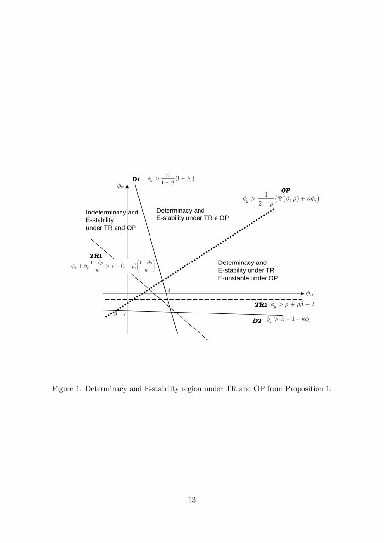
Figure 1 visualizes how the �ve conditions above de�ne the relevant regions for

determinacy and E-stability in both cases of TR and OP in the space (��; �y) implied

by Proposition 1: To grasp the main results, it is instructive to con�ne the analysis to the

positive orthant for (��; �y): To facilitate the reader, we highlight the main implications

of this proposition, by using a numbered list of results.

Result 1.1 Transparency helps anchoring in�ation expectations. Let�s ��; �y �

0: If the rational expectation equilibrium is determinate (i.e., (D1) holds), then it

is always learnable under TR, while this is not true under OP.

This follows immediately from the fact that for �y � 0 both (TR2) is always satis�ed,

and that the long-run Taylor principle (D1) implies (TR1). Note that, if the determinacy

conditions hold, then the equilibrium is learnable under TR, but the contrary is not

true, in contrast to Bullard and Mitra (2002): E-stability does not imply determinacy.15

Moreover, while determinacy implies E-stability under TR, this is not true under OP.

The learnability region of the parameter space is thus smaller under OP with respect to

TR. This reminds a similar result in Preston (2006). Using his in�nite horizon approach,

Preston (2006) shows that under OP the Taylor principle is not su¢ cient for E-stability.

However, even when agents form expectations just one-period ahead, requiring them to

15Again this is because we do not use the constant term in the PLM (see Section 3.3).

12

1y πφ β κφ> − −

Yφ

Πφ

( )11y π

κφ φ

β> −−

β − 1

1

OPOPOPOP

D1D1D1D1

D2D2D2D2

TR2TR2TR2TR2

TR1TR1TR1TR1

Indeterminacy andE-stabilityunder TR and OP

Determinacy andE-stability under TR e OP

Determinacy andE-stability under TRE-unstable under OP

2yφ ρ ρβ> + −

( )( )1

Ψ2y , πφ β ρ κφρ

> +−

( )1 - 1 -

1yπ

βρ βρφ φ ρ ρ

κ κ

+ > − −

Figure 1. Determinacy and E-stability region under TR and OP from Proposition 1.

13

learn the policy rule is an important source of instability. Hence, the di¤erence between

the Bullard and Mitra (2002) and Preston (2006) results are not due to the di¤erent

assumption regarding the forecast horizon of the expectation process under learning.

We have shown that under OP the standard Euler equation approach delivers a similar

result as in Preston (2006): the condition for E-stability are more stringent under OP.

Besides, Preston (2006) already shows that TR yields the Bullard and Mitra (2002)

result that the Taylor principle is necessary and su¢ cient for E-stability.16 So it seems

that the two approaches deliver similar results. No matter the forecast horizon of the

expectation process under learning, TR delivers E-stability if the REE is determinate,

while OP generates more instability and requires more stringent conditions.

As Eusepi and Preston (2010) in the in�nite horizon case, we were able to obtain an

analytical expression for the E-stability condition under OP. This allows us to uncover

other important implications. The next question is: which features of the monetary

policy rule make the equilibrium learnable under OP? For example, does responding

more aggressively to in�ation help to anchor in�ation expectations under OP? Quite

surprisingly, the answer is no.

Result 1.2 Under OP, monetary policy should respond to the output gap.

Let�s ��; �y � 0: If the rational expectation equilibrium is determinate (i.e., (D1)

and (D2) hold), it is learnable under OP i¤ �y >1

(2��) ((�; �) + ���) :

For the equilibrium to be learnable under OP, condition (OP) implies a lower bound

on �y that increases with ��: In other words, an aggressive response to in�ation can

destabilize expectations under OP, unless it is counteracted by an increase in the re-

sponse to output. Intuitively, if in�ation expectations increase, agents fail to anticipate

higher real rates under OP, even if the opaque central bank follows the Taylor Princi-

ple. As a result output increases leading to an increase in in�ation that validates the

initial increase in in�ation expectations. The intuition for this result in well-explained

by Eusepi and Preston (2010, p. 243-244) in an in�nite horizon framework. This is due

16In our case, it is only su¢ cient, again beacuse of di¤erent modelling assumptions about expecta-tions formations.

14

to the fact that policy responds not to current, but to expected variables.17 A strong

response to expected in�ation then tends to destabilize the economy, since monetary

policy is responding "too much and too late". The central bank can stabilize in�ation

expectations by responding relatively more to expected output, "which is a more �lead-

ing� indicator of in�ation". This result has two main implications. First, OP may be

costly, since the optimal policy literature generally suggests that it is suboptimal to

respond to the output gap.18 Second, under OP it is not true that determinacy implies

E-stability, as claimed by McCallum (2007). This result echoes similar results in Preston

(2006), Bullard and Mitra (2007) and Eusepi and Preston (2010) in the in�nite horizon

framework.

Moreover, Figure 1 clearly displays an important result: transparency is an essential

part of the in�ation targeting framework. Under pure in�ation targeting, the interest

rate rule responds only to in�ation. In that case, OP would lead either to E-instability

or to indeterminacy, depending if the Taylor principle is satis�ed or not. Thus, we can

state:

Result 1.3 A pure in�ation targeting central bank needs to be transparent to

anchor in�ation expectations.

Finally, note there is a region of the policy parameter space (��; �y) where despite

the rational expectation equilibrium being indeterminate, it is learnable under both TR

and OP. And in this particular region, the Taylor principle is not satis�ed. In general:

Result 1.4 The Taylor principle is not a necessary condition for E-stability

neither under TR nor under OP.

Having analyzed how the E-stability property depends on the policy parameters,

the next obvious question is: which structural parameters of the economy do a¤ect the

17Indeed, if we use contemporaneous expectations, there is no di¤erence between the OP and TRcase. See the robustness Section 3.3.

18This is generally true for optimal policy in a simple NK model (see Woodford, 2003). Moroever,Schmitt-Grohé and Uribe (2006) shows it in the context of a medium-scale DSGE NK model à laChristiano et al. (2005) or Smets and Wouters (2003).

15

di¤erent ability of anchoring expectations under TR and under OP? That is, which

features of the economy do make TR more necessary to anchor in�ation expectations?

First note that the slope of the NKPC (7), �, is the key parameter to interpret

determinacy. It is immediate to see that determinacy is more likely, the lower the slope

of the NKPC (see (D1) and (D2)). Recall that � = �(1+�n) and � depends (inversely)

on �. Hence, it follows that the higher the degree of price stickiness (higher �) or the

lower the elasticity of the marginal disutility from working (�n), then the lower is �; and

the larger is the determinacy region.

yφ

πφ

πφ >1

1

OPOPOPOP

D1 and TR1D1 and TR1D1 and TR1D1 and TR1

y πφ κφ>Determinate andE-stable under TR e OP

Determinate andE-stable under TRE-unstable under OP

IndeterminateandE-unstableunder TR and OP

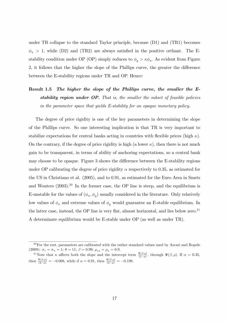
Figure 2. The importance of the slope of the Phillips curve, �:

Similarly, � is also the key parameter that a¤ects the E-stability conditions. To

clearly see this assume � = � = 1:19 Then, the determinacy and E-stability conditions19This is just for the sake of exposition without loss of generality. The same argument applies for

values 0 < �; � < 1:

16

under TR collapse to the standard Taylor principle, because (D1) and (TR1) becomes

�� > 1; while (D2) and (TR2) are always satis�ed in the positive orthant. The E-

stability condition under OP (OP) simply reduces to �y > ���: As evident from Figure

2, it follows that the higher the slope of the Phillips curve, the greater the di¤erence

between the E-stability regions under TR and OP. Hence:

Result 1.5 The higher the slope of the Phillips curve, the smaller the E-

stability region under OP. That is, the smaller the subset of feasible policies

in the parameter space that yields E-stability for an opaque monetary policy.

The degree of price rigidity is one of the key parameters in determining the slope

of the Phillips curve. So one interesting implication is that TR is very important to

stabilize expectations for central banks acting in countries with �exible prices (high �).

On the contrary, if the degree of price rigidity is high (a lower �); then there is not much

gain to be transparent, in terms of ability of anchoring expectations, so a central bank

may choose to be opaque. Figure 3 shows the di¤erence between the E-stability regions

under OP calibrating the degree of price rigidity � respectively to 0.35, as estimated for

the US in Christiano et al. (2005), and to 0.91, as estimated for the Euro Area in Smets

and Wouters (2003).20 In the former case, the OP line is steep, and the equilibrium is

E-unstable for the values of (��; �y) usually considered in the literature. Only relatively

low values of �� and extreme values of �y would guarantee an E-stable equilibrium. In

the latter case, instead, the OP line is very �at, almost horizontal, and lies below zero.21

A determinate equilibrium would be E-stable under OP (as well as under TR).

20For the rest, parameters are calibrated with the rather standard values used by Ascari and Ropele(2009): �c = �n = 1; � = 11; � = 0:99; �rn = �u = 0:9:

21Note that � a¤ects both the slope and the intercept term (�;�)(2��) ; through (�; �): If � = 0:35;

then (�;�)(2��) = �0:008; while if � = 0:91; then

(�;�)(2��) = �0:198:

17

0 0.5 1 1.5 2 2.5 3 3.5 4 4.5 5­1

0

1

2

3

4

5

φπ

φy

Determinate andE­stable under TR & OP

Detererminate andE­stable only under TR

E­stability: no communicationE­stability: transparencydeterminacy

� = 0:35

0 0.5 1 1.5 2 2.5 3 3.5 4 4.5 5­1

0

1

2

3

4

5

φπ

φy

Detererminate andE­stable under TR & OP

E­stability: no communicationE­stability: transparencydeterminacy

� = 0:91

Figure 3. E-stability regions and price stickiness

It is very important to get the intuition of why this is happening, since this will help

also understanding the results in the next section. Recall that an opaque central bank

needs to respond to output (and the more so, the more it is aggressive to in�ation),

because responding to in�ation can destabilize expectations, when agents do not know

the policy rule and the policy responds to lagged expected values, that is, with a lag.

Policy is responding "too much, too late". However, this potentially destabilizing e¤ect

under OP depends on the e¤ectiveness of the policy. In a New Keynesian model, a

change in the interest rate a¤ects in�ation, through output, via the Euler equation. It

follows that the e¤ectiveness of monetary policy rests on the link between output and

in�ation in the NKPC. If the latter is weak, then monetary policy is not very e¤ective.

If current output is not an important determinant of current in�ation, then, monetary

policy does not have destabilizing e¤ects on expectations, because it is not very e¤ective

in in�uencing the dynamics of in�ation. Thus, the E-stability region under OP enlarges

for higher values of price rigidities (low �) and, for a given ��; monetary policy could

respond less to output to deliver E-stability. Note that in the simple case of � = � = 1;

then � determines the lower bound of the relative weight�y��necessary to ensure E-

stability under OP. So, the less e¤ective is monetary policy, the more the central bank

can be opaque, simply because what it does, it matters less.

18

For the same reasons, the di¤erence between TR and OP lowers with the slope

of the Phillips curve. The less monetary policy is e¤ective, the less knowing or not

knowing the path of the interest rate makes a di¤erence. Intuitively, at the limit, if

prices are completely rigid and � = 0, monetary policy can not in�uence in�ation,

there is no advantage in knowing the policy and no di¤erence between TR and OP. On

the contrary, the interest rate path is a very valuable information when policy is very

e¤ective in a¤ecting in�ation.

3.2 Positive trend in�ation

We then move to analyze how the choice of a positive in�ation target by a central bank

changes the answer to the previous questions. In an in�ation targeting framework, it is

obvious how pivotal is to assess how the choice of the target in�uences the ability of the

central bank policy of anchoring in�ation expectations under both TR and OP.

The relevant model is made up by the �ve equations (1)-(5) described in Section

2.1. The dynamics of the model under positive in�ation target, thus, is very di¤erent

from the one of the simple two equations New Keynesian model of the previous section

(see Ascari, 2004 and Ascari and Ropele, 2009). There are two main di¤erences. First,

the in�ation target directly a¤ects the coe¢ cients of the log-linearized equations. In

particular, the higher the in�ation target, the more price-setting becomes �forward-

looking�, because higher trend in�ation leads to a smaller coe¢ cient on current output

(���) and a larger coe¢ cient on future expected in�ation (���). With high trend in�ation

the price-resetting �rm sets a higher price since it anticipates that trend in�ation will

erode its relative price in the future. Keeping up with the trending price level becomes a

priority for the �rm, that will be thus less a¤ected by current marginal costs (see Ascari

and Ropele, 2009). Consequently, if the central bank increases the in�ation target,

the short-run NKPC �attens: the in�ation rate becomes less sensitive to variations in

current output and more forward-looking. Second, a positive in�ation target adds two

new endogenous variables: �t, which is a forward-looking variable, and st, which is a

predetermined variable. The dimension of the dynamics of the system is now of fourth

19

order, so we can not have anymore analytical results, and we proceed with numerical

simulations.22 Again, we highlight the main implications of our analysis by listing a

number of results.

The �rst question then is: does the choice of a higher in�ation target undermine

the ability of the central bank to anchor in�ation expectations? The answer is yes, very

much so.

Result 2.1 If the central bank �xes a higher in�ation target, it is more dif-

�cult to anchor in�ation expectations under both TR and OP.

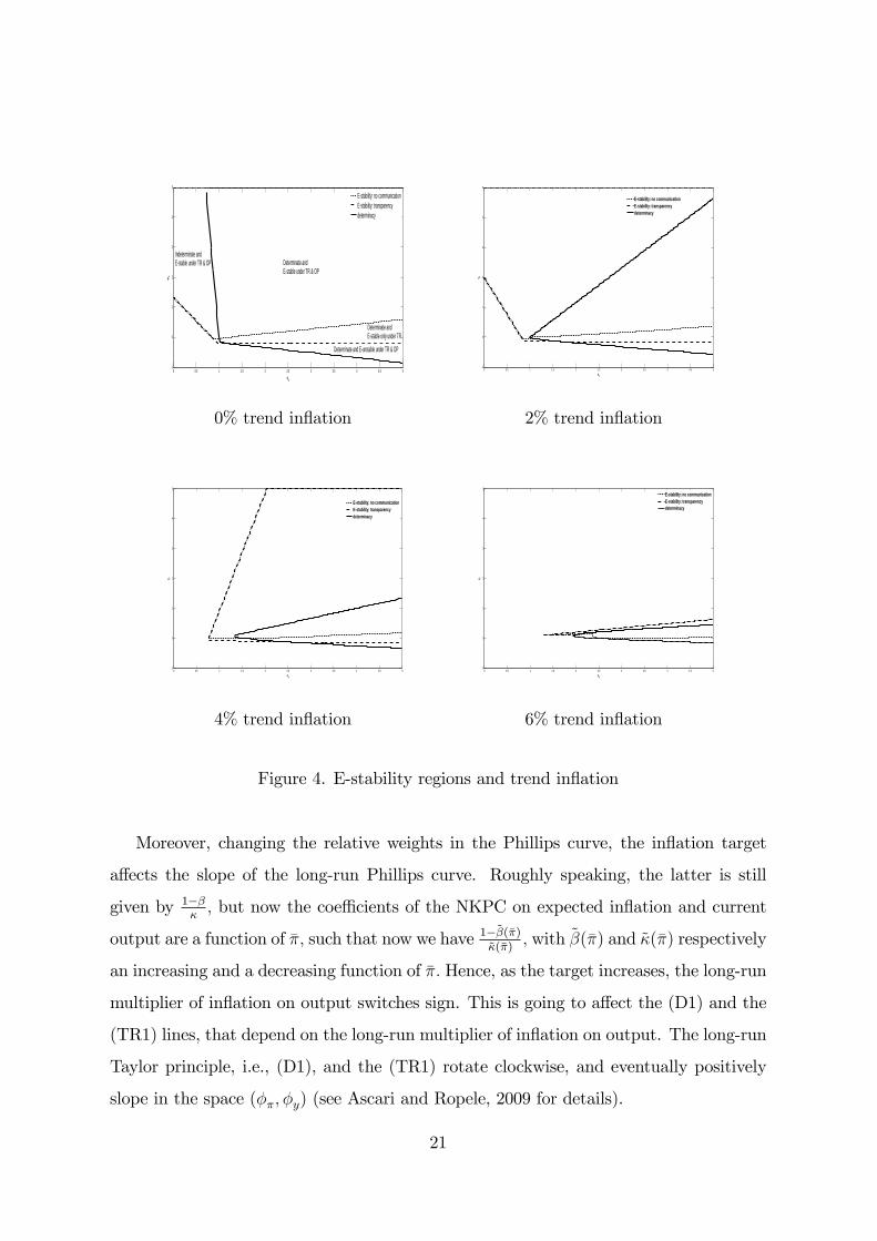
Figure 4 plots the determinacy and E-stability regions both under TR and under OP,

for four di¤erent values of trend in�ation: 0, 2%, 4% and 6%. As known, higher levels

of trend in�ation shrink the determinacy region. It turns out that higher trend in�ation

has similar e¤ects also on the conditions for E-stability under both TR and OP. Similarly

to the determinacy region, the E-stability region of the policy parameter space (��; �y)

is very sensitive to mild variations in the in�ation target and shrinks substantially even

for moderate levels of in�ation targets. Given our calibration and the considered range

for (��; �y); when the in�ation target is as high as 8% in�ation, there is no possibility

to anchor in�ation expectations and there is no E-stability region under both TR and

OP. The intuition rests on the increase in the forward-lookingness in price setting on

the part of the �rms. The NKPC coe¢ cients are now a function of the in�ation target.

As trend in�ation increases, there is a larger coe¢ cient on future expected in�ation

and a smaller coe¢ cient on current output. As a result, in�ation becomes less sensible

to output changes, and thus, monetary policy less e¤ective, making more di¢ cult to

stabilize expectations.

22Calibration is as in footnote 20 and � = 0:75:

20

0 0.5 1 1.5 2 2.5 3 3.5 4 4.5 5­1

0

1

2

3

4

5

φπ

φy

Determinate andE­stable under TR & OP

Determinate andE­stable only under TR

E­stability: no communicationE­stability: transparencydeterminacy

Determinate and E­unstable under TR & OP

Indeterminate andE­stable under TR & OP

0% trend in�ation

0 0.5 1 1.5 2 2.5 3 3.5 4 4.5 5­1

0

1

2

3

4

5

φπ

φy

E­stability: no communicationE­stability: transparencydeterminacy

2% trend in�ation

0 0.5 1 1.5 2 2.5 3 3.5 4 4.5 5­1

0

1

2

3

4

5

φπ

φy

E­stability: no communicationE­stability: transparencydeterminacy

4% trend in�ation

0 0.5 1 1.5 2 2.5 3 3.5 4 4.5 5­1

0

1

2

3

4

5

φπ

φy

E­stability: no communicationE­stability: transparencydeterminacy

6% trend in�ation

Figure 4. E-stability regions and trend in�ation

Moreover, changing the relative weights in the Phillips curve, the in�ation target

a¤ects the slope of the long-run Phillips curve. Roughly speaking, the latter is still

given by 1���; but now the coe¢ cients of the NKPC on expected in�ation and current

output are a function of ��; such that now we have 1�~�(��)~�(��)

; with ~�(��) and ~�(��) respectively

an increasing and a decreasing function of ��: Hence, as the target increases, the long-run

multiplier of in�ation on output switches sign. This is going to a¤ect the (D1) and the

(TR1) lines, that depend on the long-run multiplier of in�ation on output. The long-run

Taylor principle, i.e., (D1), and the (TR1) rotate clockwise, and eventually positively

slope in the space (��; �y) (see Ascari and Ropele, 2009 for details).

21

One main policy implication concerns the recent proposal by Blanchard et al. (2010)

to raise the in�ation target to have more room of manoeuvre to decrease the real interest

rate before hitting the zero lower bound in the case of a crisis. This proposal could hide

an important peril: the unanchoring of in�ation expectations, as suggested by Fed

Chairman Bernanke.

The next obvious questions is how the in�ation target a¤ects the di¤erent ability of

anchoring expectations under TR and OP? Does a central bank that �xes a higher level

of in�ation target need to be more transparent?

Result 2.2 If the central bank �xes a higher in�ation target, the advantage

of being TR in anchoring expectations diminishes.

Looking at the Figure 4 the line that corresponds to the condition (OP) in a positive

in�ation targeting framework �attens with trend in�ation. Thus the di¤erence between

the E-stability regions under TR and OP contracts. The intuition is the same that

explains Result 1.5 in the previous section. A higher in�ation target �attens the slope

of the Phillips curve, so it has a similar e¤ect of a decrease in � in the previous section.

If output becomes less relevant in determining current in�ation, then, even knowing the

interest rate becomes less important, because the latter a¤ects in�ation dynamics only

through current output. In other words, Result 1.2 weakens because under OP a strong

response to expected in�ation is less likely to destabilize expectations, and the central

bank can respond relatively less to expected output to stabilize in�ation expectations.

Moreover, note that looking at this result from a reverse perspective implies that TR is an

important component of the in�ation targeting approach. Central banks in developed

countries moved in the last decades to an in�ation targeting framework and greater

transaparency with the aim of lowering average in�ation. The central idea is that this

framework and a greater transparency should help coordinating and anchoring in�ation

expectations. Our result supports this view, because the lower the in�ation target, the

more TR is important (vs OP) for expectations stabilization.

The next interesting question again regards how a higher in�ation targeting shapes

the feasible monetary policy rules. Does a higher in�ation target requires monetary

22

policy to be more hawkish on in�ation and/or on output?

Result 2.3 The higher the in�ation target �xed by the central bank, the more

monetary policy should respond to in�ation under both TR and OP.

While it is still true that a pure in�ation targeting central bank needs to be trans-

parent, the minimum �� necessary to stabilize expectations increases with the in�ation

target. As Figure 4 shows, the crossing of the E-stability (as well as for determinacy)

conditions under both TR and OP moves to the right.

Result 2.4 A high in�ation target implies an upper bound for �y under both

TR and OP.

Moreover, while the lower bound for �y in case of OP reduces, because condition

(OP) �attens with trend in�ation (see Result 2.2), in contrast with the zero in�ation

target case, a higher in�ation target actually generates an upper bound for �y, because

of the clockwise rotation of the (TR1), as the long-run relationship between output and

in�ation becomes negative. Hence, a too strong reaction to expected output gap may

destabilize expectations by increasing in�ation in the future.

It follows that if, for whatever reasons, the Fed had to adopt a higher in�ation

target, it would need to be more aggressive on in�ation and responds less to output.

It would be unwise to suggest a policy that would increase the in�ation target and

contemporaneously respond less to in�ation and output.

To conclude, the level of the in�ation target has substantial e¤ects on the E-stability

regions and hence on the ability of a central bank to control in�ation expectations. The

higher the target in�ation rate: (i) the more di¢ cult is to anchor expectations, (ii) the

less a central bank needs to be transparent; (iii) the more hawkish on in�ation a central

bank should be.

3.3 Robustness

In this section we investigate the robustness of our results along di¤erent dimensions.

23

Policy Rule. First, we investigate if and how results change when we modify

the policy rule. The determinacy properties are basically the same as in Ascari and

Ropele (2009). Regarding E-stability, while a forward looking policy rules does not

alter the E-stability region with respect to the benchmark case, a backward looking

policy rule is quite di¤erent because it always returns E-stability under both TR and

OP. These results are di¤erent from Kobayashi and Muto (2011) because of the di¤erent

assumptions regarding the learning process (see below).

When one considers the more realistic case of a Taylor rule that includes a lagged

interest rate to account for interest rate smoothing by the central bank, then, as the

degree of interest rate smoothing increases, the determinacy and the E-stability regions

widen for every value of the in�ation target considered.23 This is in line with previous

results that show that interest rate inertia enlarges the determinacy region both under

zero (e.g., Woodford, 2003) or positive trend in�ation (e.g., Ascari and Ropele, 2009),

and promotes learnability (Bullard and Mitra, 2007). Moreover, we �nd that, as trend

in�ation increases, the E-learnable region shrinks much more slowly (if compared to the

baseline case). According to our usual calibration, in the presence of smoothing, the

anchoring of expectations becomes now a possibility even for values of in�ation target

as high as 8%. So we can con�rm that inertia do promotes learnability and stability of

the REE even for fairly high levels of trend in�ation. Moreover, as the inertia parameter

approaches the value of one, if one con�nes the analysis to the positive orthant (��; �y),

the di¤erence between TR and OP disappears. With high inertia, in fact, the interest

rate today is close to the previous period�s one hence there is no need to make learning

on it: this lowers the bene�t of TR.

In any case, the main message of the paper goes through: higher trend in�ation

tends to unanchor in�ation expectations making learnability more di¢ cult.

Learning assumptions. Second, we also investigate the robustness of our results

to our assumptions regarding the speci�cation of learning in our model. If we introduce

in the PLM a constant term, as in the pivotal paper by Bullard and Mitra (2002), the

main results are largely una¤ected. The only change, under a zero in�ation target, is the

23With the e¤ect larger on the E-stability zone.

24

coincidence of the "long run" Taylor principle (D1) and the E-stability condition (TR1).

As trend in�ation increases these two conditions separate. They remain, however, closer

to each other if compared to the baseline case.

The hypothesis that changes most our results is the one about expectation formation.

Under contemporaneous expectations, the determinacy and E-stability regions in the

positive orthant (��; �y) do not change if compared to the baseline case. However,

any di¤erence between TR and OP vanishes. In this case there is no central bank�s

information fruitfully exploitable by the public.

Model structure. Third, we examine the e¤ects of including price indexation.

It is well-known that indexation counteracts the e¤ects of trend in�ation. We �nd

that this is true both regarding determinacy, as in Ascari and Ropele (2009), and E-

stability. We consider the two cases most familiar from the literature: trend in�ation

and backward-looking indexation (e.g., Christiano et al., 2005). Regarding E-stability,

there is no substantial di¤erence between these two cases. The e¤ects of trend in�ation

are partially o¤set by indexation, so that as trend in�ation increases the E-stability

frontiers shifts less with respect to the benchmark case. Partial indexation makes the

slope of the Phillips curve less sensitive to trend in�ation, because price setters need

to a less extent to set very high prices in order to take into account the presence of

trend in�ation. They are then more sensitive to current marginal costs and economic

conditions. As suggested by Result 2.2, this reestablishes the importance of TR.

Finally, we discuss some implications for the degree of price rigidity. More �exibility

(lower �) makes both the determinacy and the E-stability frontier close less rapidly

compared with the baseline case, because trend in�ation matters less the more �exible

are the prices. Moreover, recall from Figure 3 that a lower degree of price rigidity

implies a larger di¤erence between TR and OP, because the OP line is quite sensitive

to the degree of price rigidity. However, � may not be considered a truly structural

parameter, and it could decrease with trend in�ation (see Levin and Yun, 2007). In

other words, �rms would change their price more often (i.e., increase price �exibility) as

trend in�ation increases. As a results, there could be two possible forces acting on the

(OP) line as trend in�ation changes. On the one hand, higher trend in�ation �attens

25

the (OP) line moving it towards the (TR2) line; on the other hand, if trend in�ation

causes a lower �; higher price �exibility shifts the (OP) line upwards, moving it away

from (TR2) and shrinking the E-stability region under OP. Which of the two forces will

prevail depends on calibration and on the eventual elasticity of � with respect to trend

in�ation. If the latter e¤ect prevails, then, Result 2.2 can be overturned and as trend

in�ation increases there would be a greater need for TR.

Robustness on the other calibration parameters do not qualitatively alter our main

results. Decreasing the value of the elasticity of substitution (�) or increasing the in-

tertemporal elasticity of labour supply (�n) makes the di¤erence between TR and OP

shrink slower as trend in�ation rises. All the above results are available upon request.

4 Speed of convergence

The previous analysis focused on the asymptotical properties of the learning process, by

determining the conditions for the E-learnability of the REE. Following Ferrero (2007),

we also analyze how monetary policy can a¤ect the transitional properties of the learning

process, by studying the speed of convergence of expectations to the REE. The speed of

convergence matters because a fast convergence means that the economy, and thus its

dynamics, would always be very close to the REE, while a slow convergence implies that

economic dynamics would be dominated by the transitional dynamics under learning.

As such, the speed of convergence could also well be another criteria to judge a given

policy.

To analyze the speed of convergence, it is obviously needed to assume convergence

to a unique REE, that is the analysis is conducted in the E-stability and determinacy

region of the parameter space. The speed of convergence is then determined by the

properties of the same ODE employed to value E-stability, that is, the T-mapping from

PLM to ALM. In particular, the speed of convergence is determined by the spectral

radius (i.e., the largest eigenvalue in absolute value) of the derivative of the T-map (see

Ferrero, 2007, and Ferrero and Secchi, 2010). To converge, all the eigenvalues need to

be within the unit circle, and the larger the spectral radius, the slower the convergence.

26

Indeed, when the largest eigenvalue crosses the unit circle, then the economic dynamics

cross into the E-unstable region of the parameter space and there is no convergence

anymore to the REE. Rather than simply referring to the eigenvalue, we actually o¤er a

measure of the speed of convergence. Given the spectral radius of the derivative of the

T-map, one can estimate the number of iterations necessary to reduce the initial error

by a certain amount, say one-half, to conform to the common half-life measure. The

measure of speed we then plot is simply the inverse of this number of iterations (this

should be intended as an asymptotic rate of convergence, see Appendix).

We now study the speed of convergence �rst in the zero in�ation target case and

then under positive trend in�ation.24

4.1 Zero in�ation target

Figure 5 displays the iso-speed curves25 in the case of, respectively, TR and OP. Since

the speed of convergence can be calculated just in the E-stability region and this region

is smaller under OP, this is re�ected into a more acute angle of the iso-speed curves. The

two �gures convey the same message. Recall from Figure 1 the shape of the region that

is both E-stable and determinate in the two cases of OP and TR. When the policy is such

that the economy is close either to the E-stability frontier (lower frontier on the right)

or the determinacy frontier (upper frontier on the left), then the T-map spectral radius

is approaching unity. Thus close to the frontiers the convergence speed is low. On the

contrary, when the policy is such that the economy is well within the boundaries then the

largest eigenvalue bottoms out and the speed of convergence is high. In other words, to

get a higher speed one needs to remain well within the determinacy/E-stability region,

while keeping away from its frontiers. Thus, Figure 6 shows that the 3-D graph of the

speed of convergence as a function of the policy parameters (��; �y) is like a mountain

with a ridge that runs in the middle of the region described by the E-stablility and

determinacy frontier. The di¤erence between the two cases of OP and TR then rests

24Calculations of the speed of convergence are based on simulations obtained under the usual para-meter calibration (see footnotes 20 and 22).

25An iso-speed curve is de�ned by the combinations of parameter values that deliver the same largesteigenvalue in absolute value.

27

on the di¤erence between these two regions, as described in Figure 1. With the help of

Figure 5 and 6 and Table 2 we can answer questions relating to the speed of convergence

in the same vein as the previous Sections.

First: does TR allow a central bank to increase the speed of convergence with respect

to OP? The TR surface in Figure 6 lies almost always well above the OP one, thus

signaling a higher speed of convergence, unless for a limited region of the parameter

space where anyway the di¤erence is minor. The maximum speed of convergence under

TR is much higher than under OP. So we can conclude that transparency helps increase

the speed of convergence.

Second, how does policy a¤ect the speed of convergence? To get the quickest conver-

gence, policy has to move towards the centre of the determinacy/E-stability region, that

is, to be on the ridge. Note that the ridge runs across that region, so that to increase

the speed of convergence both �� and �y have to increase at the same time both in the

case of OP and TR. A stronger reaction both to in�ation and to the output gap seems

to give more informations to the agents, speeding up the learning process. As in the

previous Section, in the OP case it is again the ratio �y/�� that matters: the ridge is

almost linear and loosely described by a ratio �y/�� � 0:5 (see Figure 5). Moreover, in

the TR case, the speed is not decreasing with ��. For each level of �y, the speed is �rst

increasing for low values of ��, till it reaches a ceiling, where further increases in the

reaction of the policy to in�ation would not have any e¤ect on the speed of convergence.

An interesting particular case is the one of a pure in�ation targeting central bank. We

have already pointed out the need of transparency by a pure in�ation targeting central

bank. In this particular case, under TR and �y = 0; the speed is constant, that is inde-

pendent from ��; and it depends just on the autoregressive component of the exogenous

disturbance terms (assuming these are equal). So, under pure in�ation targeting the

central bank cannot a¤ect the (low) speed of convergence.

We are actually able to prove these results in the case of transparency through the

following Proposition (proof in Appendix).

Proposition 2 In the case of TR and zero trend in�ation, the speed of convergence:

(i) does not depend on �� i¤��(� � 1) + �y

�2 � 4�(�� � �) and it is strictly increasing28

otherwise;

(ii) is decreasing with �y i¤��(� � 1) + �y

�2> 4�(�� � �) and �(� � 1) + �y > 0 and

�� > �; while it is increasing with �y otherwise;

(iii) does not depend on � i¤��(� � 1) + �y

�2 � 4�(�� � �); it is decreasing in � i¤��(� � 1) + �y

�2> 4�(�� � �) and �� < �; while it is increasing i¤

��(� � 1) + �y

�2>

4�(�� � �) and �� > �:0.

20.

2

0.2 0.2 0.2

0.4

0.4

0.4 0.4 0.4

0.6

0.6

0.6 0.6 0.6

0.8

0.8

0.8 0.8 0.8

1

1

1 1

1.5

1.5

1.5

2

2

2.5

2.5

3

φπ

φ y

Transparency

0 0.5 1 1.5 2 2.5 3 3.5 4 4.50

0.2

0.4

0.6

0.8

1

1.2

1.4

1.6

1.8

0.1

0.1

0.1

0.1

0.1

0.2

0.2

0.2

0.2

0.2

0.3

0.3

0.3

0.3

0.3

0.4

0.4 0.4

0.4

0.4

0.5

0.5

0.5

0.5

0.5

0.6

0.6

0.6

0.6

0.6

0.7

0.7

0.7

0.7

0.7

φπ

φ y

Opacity

0 0.5 1 1.5 2 2.5 3 3.5 4 4.50

0.2

0.4

0.6

0.8

1

1.2

1.4

1.6

1.8

Figure 5. Iso-speed curves

29

Table 2. Speed of convergence S = � log2(spectral radius)

trend in�ation 0% �y 0 0.5 1

�� OP TR OP TR OP TR

1.5 - 0.15 0.37 0.62 0.47 0.38

2 - 0.15 0.25 0.62 0.71 0.67

3 - 0.15 0.12 0.62 0.43 1.32

trend in�ation 2% �y 0 0.5 1

�� OP TR OP TR OP TR

1.5 0 0.12 0.30 0.23 - -

2 - 0.12 0.42 0.43 0.23 0.20

3 - 0.14 0.22 0.49 0.40 0.38

Figure 6. Speed of convergence under opacity and transparency with zero in�ation

target

30

4.2 Positive in�ation

What is the e¤ect of a positive in�ation target on the speed of convergence? Figures

7a,b (TR case) and 7c (OP case) clearly show the main result of this section: a higher

in�ation target tends to lower the speed of convergence of expectations under learning to

the REE both under OP and under TR. For our parameterization, this is always true

in the case of TR, where the di¤erence between a zero and a 2% in�ation target is very

large.26 In the latter case the speed is never higher than 0.4, while in the former case it

reaches 2.7 and it is higher than 0.4 for most of the policy parameter values. The shape

of the surfaces in Figure 7 are qualitatively similar, but trend in�ation pushes the ridge

down to a great extent. Thus, even a very modest increase in the in�ation target has

large e¤ects on the speed of convergence of expectations under learning. As such, the

values of the convergence speed become close to the OP case. Thus, the advantage of

being transparent (the di¤erence between being OP and TR), in terms of the speed of

convergence, decreases as trend in�ation increases. In the OP case, the speed is already

quite low at zero in�ation, so the e¤ects of trend in�ation are qualitatively similar to

the case of TR, but less pronounced. Trend in�ation does not change qualitatively the

e¤ects of policy parameters on the speed: to increase the speed, policy makers have

to increase both �� and �y; under pure in�ation targeting and positive trend in�ation,

the central bank can (barely) a¤ect the (very low) speed of convergence increasing ��.

However, these e¤ects are now much less marked given that the ridge is much lower than

in the zero trend in�ation case.

This is no surprise, given that: (i) a higher in�ation target shrinks the E-stability /

determinacy frontier; (ii) the speed of convergence is lower the closer the economy is to

these frontiers. A higher in�ation target increases the spectral radius of the derivative

of the T-map, such that, ceteris paribus, both the speed of convergence of expectations

is lower under E-stability, and the learning dynamics are more likely to be E-unstable.

26In fact, we add Figure 7b in order to appreciate the surfaces in the case of 2% and 4% in�ationtarget. In Figure 7a, those surfaces can not be visualized because the di¤erence between them and theone relative to the zero trend in�ation case is large.

31

7a: Transparency

7b: Transparency32

7c Opacity

Figure 7. Speed of convergence for di¤erent values of trend in�ation under opacity and

transparency

5 Conclusions

This paper supports the claim that a higher in�ation target unanchors expectations,

as often suggested by Fed Chairman B. Bernanke. We investigate a New Keynesian

model that allows for trend in�ation under adaptive learning, in the spirit of Evans and

Honkapohja (2001). Technically, a higher in�ation target increases the spectral radius

of the matrix that de�nes the T-map under adaptive learning, and that governs the

convergence of the learning algorithm. Hence, we were able to show that, when a central

bank follows a Taylor rule, the higher the in�ation target, the smaller the E-stability

region and the speed of convergence of the expectations to the rational expectation

equilibrium under E-stability. Moreover, the higher the in�ation target, the more the

33

policy should be hawkish with respect to in�ation to stabilize expectations, while it

should not respond too much to output. This result questions the argument that the

Fed should increase the in�ation target and, contemporaneously, ease monetary policy

to respond to the surge in unemployment. Our results suggest that this policy would

indeed be "reckless" and "unwise", as Bernanke recently said.

Moreover, our results con�rm the claim that transparency is an essential component

of the in�ation targeting framework. The paper looks at the distinction between TR

and OP. When a central bank is transparent, agents know the policy rule and use it

in forming expectations (see Preston, 2006). When a central bank is opaque, instead,

agents need to learn also the policy rule. We �nd that transparency helps in anchoring

expectations, that is, the E-stability region is wider under transparency than under

opacity for all the possible Taylor rules and in�ation targets. Moreover, a pure in�ation

targeting central bank needs to be transparent to anchor in�ation expectations. Finally:

the more �exible are the prices, the more transparency is valuable; and under opacity,

a more aggressive response to in�ation could destabilize in�ation expectations, while a

larger response to output tends to stabilize them.

34

References

Ascari, G. (2004). Staggered prices and trend in�ation: Some nuisances. Review of

Economic Dynamics 7, 642�667.

Ascari, G. and T. Ropele (2009). Trend in�ation, taylor principle and indeterminacy.

Journal of Money, Credit and Banking 41 (8), 1557�1584.

Berardi, M. and J. Du¤y (2007, March). The value of central bank transparency when

agents are learning. European Journal of Political Economy 23 (1), 9�29.

Blanchard, O., G. Dell�Ariccia, and P. Mauro (2010). Rethinking macroeconomic

policy. Journal of Money, Credit and Banking 42 (s1), 199�215.

Branch, W. A. and G. W. Evans (2011). Unstable in�ation targets. mimeo.

Bullard, J. B. and K. Mitra (2002). Learning about monetary policy rules. Journal of

Monetary Economics 49, 1105�1129.

Bullard, J. B. and K. Mitra (2007). Determinacy, learnability, and monetary policy

inertia. Journal of Money, Credit and Banking 39 (5), 1177�1212.

Christiano, L. J., M. Eichenbaum, and C. L. Evans (2005). Nominal rigidities and

the dynamic e¤ects of a shock to monetary policy. Journal of Political Econ-

omy 113 (1), 1�45.

Cogley, T., C. Matthes, and A. M. Sbordone (2010). Optimal disin�ation under learn-

ing. mimeo.

Cogley, T. and A. M. Sbordone (2008). Trend in�ation, indexation and in�ation per-

sistence in the New Keynesian Phillips Curve. American Economic Review 98 (5),

2101�2126.

Coibion, O., Y. Gorodnichenko, and J. F. Wieland (2010). The optimal in�ation rate

in New Keynesian models. NBER Working Paper No. 16093.

Eusepi, S. and B. Preston (2010). Central bank communication and expectations

stabilization. American Economic Journal: Macroeconomics 2 (3), 235�71.

35

Evans, G. W. and S. Honkapohja (2001). Learning and Expectations in Macroeco-

nomics. Princeton, New Jersey: Princeton University Press.

Evans, G. W. and S. Honkapohja (2013). Learning as a rational foundation for macro-

economics and �nance. In R. Frydman and E. S. Phelps (Eds.), Rethinking Expec-

tations: The Way Forward for Macroeconomics, Chapter 2. Princeton University

Press.

Ferrero, G. (2007). Monetary policy, learning and the speed of convergence. Journal

of Economic Dynamics and Control 31, 3006�3041.

Ferrero, G. and A. Secchi (2010). Central banks�macroeconomic projections and

learning. Banca d�Italia, Temi di discussione (Working papers) No. 782.

Galì, J. (2008). Monetary Policy, In�ation and the Business Cycle. Princeton Uni-

versity Press.

Honkapohja, S., K. Mitra, and G. W. Evans (2011). Notes on agents�behavioral rules

under adaptive learning and studies of monetary policy. CDMA Working Paper

Series 1102, Centre for Dynamic Macroeconomic Analysis.

Kobayashi, T. and I. Muto (2011). A note on expectational stability under non-zero

trend in�ation. forthcoming in Macroeconomic Dynamics.

Levin, A. and T. Yun (2007, July). Reconsidering the natural rate hypothesis in a

new keynesian framework. Journal of Monetary Economics 54 (5), 1344�1365.

McCallum, B. T. (2007). E-stability vis-a-vis determinacy results for a broad class

of linear rational expectations models. Journal of Economic Dynamics and Con-

trol 31 (4), 1376�1391.

Preston, B. (2005). Learning about monetary policy rules when long-horizon expec-

tations matter. International Journal of Central Banking 1 (2), 81�126.

Preston, B. (2006). Adaptive learning, forecast-based instrument rules and monetary

policy. Journal of Monetary Economics 53 (3), 507�535.

Sbordone, A. M. (2007). In�ation persistence: alternative interpretations and policy

implications. Sta¤ Reports 286, Federal Reserve Bank of New York.

36

Schmitt-Grohé, S. and M. Uribe (2006). Optimal �scal and monetary policy in a

medium-scale macroeconomic model. In M. Gertler and K. Rogo¤ (Eds.), NBER

Macroeconomics Annual, pp. 383�425. Cambridge, MA: MIT Press.

Schmitt-Grohé, S. and M. Uribe (2010). The optimal rate of in�ation. In B. M. Fried-

man and M. Woodford (Eds.), Handbook of Monetary Economics, Chapter Volume

3B, pp. 653�722. San Diego CA: Elsevier.

Smets, F. and R. Wouters (2003). An estimated dynamic stochastic general equilib-

rium model of the euro area. Journal of the European Economic Association 1,

1123�1175.

Woodford, M. (2003). Interest and Prices: Foundations of a Theory of Monetary

Policy. Princeton, NJ: Princeton University Press.

37

Table 1. Parameters and basic symbols

Parameters Description

� Subjective discount factor

�n Intertemporal elasticity of labour supply

� Dixit-Stiglitz elasticity of substitution

� Calvo probability not to optimize prices

�� Central Bank�s in�ation target (or trend in�ation)

�� In�ation coe¢ cient in the Taylor rule

�y Ouput coe¢ cient in the Taylor rule

NKPC Coe¢ cients

���[1����(��1)][1������]

��(��1)

��� � (�� � 1)�1� ���(��1)

����

����(��1)(���1)1����(��1)

38

A Appendix

A.1 The Model

The model is based on Ascari and Ropele (2009).

Households. Households live forever and their expected lifetime utility is:

E0

1Xt=0

�t�logCt � �

N1+�nt

1 + �n

�, (8)

where � 2 (0; 1) is the subjective rate of time preference, E0 is the expectation operator

conditional on time t = 0 information, C is consumption, N is labour, � and �n are

parameters. The period budget constraint is given by:

PtCt +Bt � PtwtNt + (1 + it�1)Bt�1 + Ft (9)

where Pt is the price of the �nal good, Bt represents holding of bonds o¤ering a one-

period nominal return it, wt is the real wage, and Ft are �rms�pro�ts rebated to house-

holds. The households maximize (8) subject to the sequence of budget constraints (9),

yielding the following �rst order conditions:

wt = �N�nt Ct, (10)

1

Ct= �Et

�1

Ct+1

(1 + it)PtPt+1

�. (11)

Final Good Producers. In each period, a �nal good Yt is produced by perfectly

competitive �rms, using a continuum of intermediate inputs Yi;t indexed by i 2 [0; 1]

and a standard CES production function Yt =hR 10Y(��1)=�i;t di

i�=(��1), with � > 1. The

�nal good producer demand schedule for intermediate good quantities is: Yi;t : Yi;t =

(Pi;t=Pt)�� Yt. The aggregate price index: Pt =

hR 10P 1��i;t di

i1=(1��).

Intermediate Goods Producers. Yi;t are produced by a continuum of �rms in-

dexed by i 2 [0; 1] : The production function for intermediate input �rms is: Yi;t = Ni;t:

Intermediate goods producers sets prices according to the usual Calvo mechanism. In

39

each period there is a �xed probability 1 � � that a �rm can re-optimize its nominal

price, i.e., P �i;t. With probability �, instead, the �rm may either keep its nominal price

unchanged . The �rst order condition of the problem is:

P �i;tPt

=�

� � 1EtP1

j=0 (��)j�

CtCt+j

��PtPt+j

���Yt+jwt+j

EtP1

j=0 (��)j�

CtCt+j

��PtPt+j

�1��Yt+j

. (12)

The aggregate price level evolves as

Pt =h� (Pt�1)

1�� + (1� �)�P �i;t�1��i1=(1��)

. (13)

As shown by Ascari and Ropele (2009), we will assume that for given parameter

values of 0 6 � < 1, 0 < � < 1, 0 6 " 6 1 and � > 1, the positive level of trend in�ationful�ls the restrictions: 1 6 �� <

�1�

� 1��1 and 1 6 �� <

�1��

� 1�, to ensure existence of the

steady state of the model (see Ascari and Ropele, 2009 for details).

Relative price dispersion. At the level of intermediate �rms, it holds true that

(Pi;t=Pt)�� Yt = Ni;t. Aggregating this expression for all the �rms i yields Ytst = Nt,

where st �R 10(Pi;t=Pt)

�� di and Nt �R 10Ni;tdi. The variable st measures the relative

price dispersion across intermediate �rms. st is bounded below at one and it represents

the resource costs (or ine¢ ciency loss) due to relative price dispersion under the Calvo

mechanism. st evolves as

st = (1� �)�P �i;tPt

���+ � (�t)

� st�1, (14)

where �t = Pt=Pt�1 denotes the gross in�ation rate. The variable st directly a¤ects the

real wage via the labour supply equation (10): wt = �Y�nt s�nt Ct.

Market clearing conditions. The market clearing conditions in the goods and

labour markets are: Yt = Ct; Y si;t = YDi;t = (Pi;t=Pt)

�� Yt, 8i; and Nt =R 10Ni;tdi.

A.2 Learning

We write our problem as:

40

yt = �0E�t�1yt + �1E

�t�1yt+1 + �yt�1 + kwt (15)

wt = 'wt�1 + et

where yt is the vector of endogenous variables and wt are the shocks (exogenous) and

et white noise. According to EH�s notation the MSV solution is written as:

yt = byt�1 + cwt�1 + ket; (16)

where the matrices b; c are to be determined.

Following Evans and Honkapohja (2001) we assume that agents�perceived law of mo-

tion (PLM) coincides with the system�s MSV solution. In this case, even the PLM will

not contain any constant term.27 Agents are assumed to know just the autocorrelation

of the shocks but they have to estimate remaining parameters.

Once the MSV solution is determined one can apply the E-stability criterion in

Proposition 10.1 of Evans and Honkapohja (2001). An MSV solution b; c to (15) is

E-stable if:

(i) all the eigenvalues of DTb(b) have real parts less than 1.

(ii) all the eigenvalues of DTc(b; c) have real parts less than 1.

Assuming none of the eigenvalues has real part equal to 1, the solution is not E-stable

if any of conditions (i), (ii) do not hold. In other words, we have stabilising expectations

or E-stability when expectations converge to REE.

In order to determine the matrices DTb(b) and DTc(b; c) one has to proceed with the

following steps. Starting from the PLM one can compute the following expectations:

E�t�1yt = byt�1 + cwt�1 (17)

27Using a PLM with a constant term, our main conclusions do not change. Results are availablefrom the authors upon request.

41

and

E�t�1yt+1 = bE�t�1yt + cE

�t�1wt = b

2yt�1 + (bc+ c')wt�1: (18)

Substituting these computed expectations into model (15) one obtains the actual law of

motion (ALM):

yt = (�1b2 + �0b+ �)yt�1 + (�0c+ �1bc+ �1c'+ �')wt�1 + ket (19)

The mapping from the PLM to the ALM takes the form

T (b; c) =��1b

2 + �0b+ �; �0c+ �1bc+ �1c'+ �'�: (20)

Expectational stability is then determined by the matrix di¤erential equation

d

d�(b; c) = T (b; c)� (b; c): (21)

The �xed points of equation (21) give us the MSV solution (b; c). The derivatives of the

T-map are:28

DTb(b) = b0 �1 + I (�0 + �1b) (22)

DTc(b; c) = '0 �1 + I (�0 + �1b) ; (23)

where I denotes an identity matrix of conformable size.

A.3 Analytical results

A.3.1 Proposition 1.

With zero tren in�ation (� = 1) and ��� = ��� = 0, the model reduces to :

�t = �E�t�1 (�t+1) + �yt + �ut

yt = E�t�1yt+1 � E�t�1 ({t � �t+1) + rnt

28See Evans and Honkapohja (2001, p.231-232) for details.

42

Transparency

�t = �E�t�1 (�t+1) + �yt + �ut

yt = E�t�1yt+1 � E�t�1(���t + �yyt) + E�t�1�t+1 + rnt

the above system can be written as follows:

yt = �0 �E�t�1yt+ �1 �E�t�1yt+1+ � � yt�1+ k �wt with wt = �wt�1+ et (1A)

the MSV solution will be29

PLM yt = cwt�1 + ket

Put the PLM into (1A) and get the ALM:

yt = �0 � cwt�1 + �1 � c�wt�1 + k � �wt�1The T-map will thus be:

T (c) = (�0c+ �1c�+ k�)wt�1

For E-stability we require the eigfenvalues of DTc(c) = �0 + �1� to have real parts

less than one.

Thus, in order to have E-stability, the eigenvalues of the matrix �0 + �1� � I, that

is:

(DTc(c)� I) =

�������� � 1 �

�� �� �� �y � 1

������must have negative real parts. This is true if the following conditions hold:30

TR1: �� + �y1����> �� (1� �)

�1����

�TR2: �y > �+ ��� 2

Hence, TR2 is always veri�ed if �y � 0.

Further, remember that the determinacy conditions (Ascari and Ropele (2009)) are:

D1: �� + �y1���> 1

D2: �� +1��y >

��1�

Note that if, as we assume, 0 < �; � < 1 if D1 is veri�ed even TR1 holds.

Opacity

{t = ��E�t�1�t + �yE

�t�1yt

�t = �E�t�1 (�t+1) + �yt + �ut

29Consider the more general formulation (yt = a + byt�1 + cwt�1 + ket) with a = 0, since there isno constant and byt�1 = 0, since b depends just on the predetermined variable s that, in this case, isabsent.

30The characteristic polynomial is X2+��y � �� ��+ 2

�X �

�� (�� ��) + (��� 1)

��y � �+ 1

��43

yt = E�t�1yt+1 � Et�1 ({t � �t+1) + rnt

Put this system in (1A) form.You get, as before, that in order to have E-stability,

the eigenvalues of the matrix �0 + �1�� I, that is:

(DTc(c)� I) =

����������1 �� �y

0 �� � 1 �

�1 � �� 1

���������must have negative real parts. This is true if the following conditions hold:31

OP1: 3� ��� � > 0

OP2: �� + �y1����> �� (1� �)

�1����

�OP3: (3� ��� �) �

��y � ��� ��+ (�� 1) (��� 2) + 1

�>���� � �y �

��y � ��

�(��� 2) + (�� 1) (��� 1)� �� (��� 1)

�Note that OP1 is always true, OP2 coincides with TR1 and OP3 (hencefort OP) can

be written as:

�y >1

(2� �) ((�; �) + ���) ; (OP)

where (�; �) = (�+ ��� 2) ((2� ��) (2� �)� ��) :

A.3.2 Speed of convergence

The spectral radius (i.e., the largest eigenvalue) of the matrix T governs the speed of

convergence in an iterative expression as:

x(k+1) = Tx(k) + d:

Assuming that xk converges to a �x point x� : limk!1

xk = x�; where x� = Tx� + d; and

de�ning the error after k iterations equal to e(k) = x��x(k); then k e(k) k�k T k kk e(0) k;

where k T k k gives the reduction in the error after k steps. Consider the geometric mean31The characteristic polynomial is: X3 + (3� ��� �)X2 +

��y � ��� ��+ (�� 1) (��� 2) + 1

�X +

���� � �y �

��y � ��

�(��� 2) + (�� 1) (��� 1)� �� (��� 1)

�

44

of the error reductions

�k =

�k e(1) kk e(0) k

k e(2) kk e(1) k :::

k e(k) kk e(k�1) k

�1=k=

�k e(k) kk e(0) k

�1=k��k T k k

�1=k:

But Gelfand�s formula shows that the spectral radius of A gives the asymptotic growth

rate of the norm:

�(T ) = limk!1

�k T k k

�1=k= lim

k!1�k;

where �(T ) is the spectral radius of the matrix. So we can de�ne an asymptotic rate of

convergence:

S1 = � log2 �(T ):

Infact to estimate the number of iterations needed for ke(k)kke(0)k �

12; that is to half the

initial error, we can use�ke(k)kke(0)k

�1=k��k T k k

�1=k= �(T ); so that

�(T )k � 1

2) k ' � 1

log2 �(T )=

1

S1:

A.3.3 Proposition 2

Under transaparency, DTc(c) :24 �� �

�� �� �� �y

35and the spectral radius is given by: � =

�(1+�)��y+q(�(��1)+�y)

2+4�(����)

2.

Part (i)

1) If��(� � 1) + �y

�2 � 4�(�� � �); real part =�(1+�)��y

2; so it follows, @�

@��= 0;

since �� does not a¤ect the real part of the eigenvalue

2) If the eigenvalue is real it follows immediately that @�@��

< 0

Part (ii)

1) If��(� � 1) + �y

�2 � 4�(�� � �); real part = �(1+�)��y2

; so it follows, @�@�y

< 0

2) If��(� � 1) + �y

�2> 4�(�� � �) :

@�@�y

= �1 + (�(��1)+�y)q(�(��1)+�y)

2+4�(����)

45

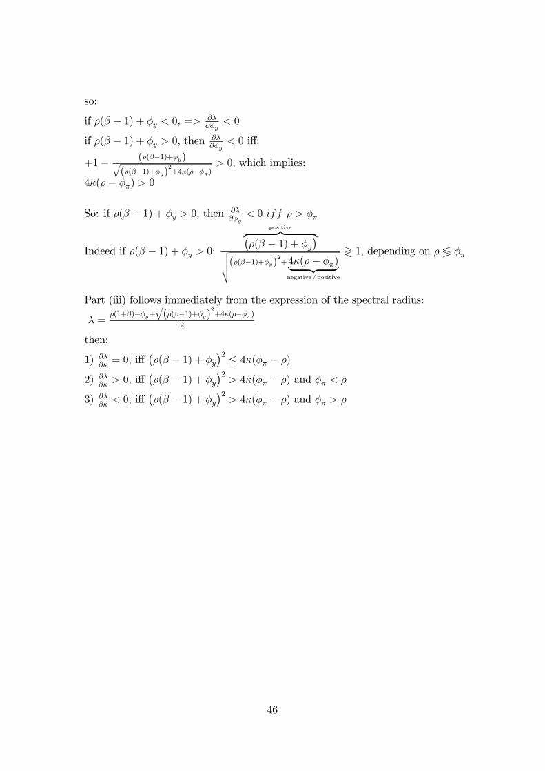
so:

if �(� � 1) + �y < 0; => @�@�y

< 0

if �(� � 1) + �y > 0; then @�@�y

< 0 i¤:

+1� (�(��1)+�y)q(�(��1)+�y)

2+4�(����)

> 0; which implies:

4�(�� ��) > 0

So: if �(� � 1) + �y > 0; then @�@�y

< 0 iff � > ��

Indeed if �(� � 1) + �y > 0:

positivez }| {��(� � 1) + �y

�vuuut(�(��1)+�y)2+4�(�� ��)| {z }

negative = positive

? 1; depending on � 7 ��

Part (iii) follows immediately from the expression of the spectral radius:

� =�(1+�)��y+

q(�(��1)+�y)

2+4�(����)

2

then:

1) @�@�= 0; i¤

��(� � 1) + �y

�2 � 4�(�� � �)2) @�

@�> 0; i¤

��(� � 1) + �y

�2> 4�(�� � �) and �� < �

3) @�@�< 0; i¤

��(� � 1) + �y

�2> 4�(�� � �) and �� > �

46