translating safe petri nets to statecharts in a structure
TRANSCRIPT
Translating Safe Petri Nets to Statecharts in aStructure-Preserving Way
Rik Eshuis
Eindhoven University of Technology, School of Industrial EngineeringP.O. Box 513, 5600 MB Eindhoven, The Netherlands
Abstract. Statecharts and Petri nets are two popular visual formalismsfor modelling complex systems that exhibit concurrency. Both formalismsare supported by various design tools. To enable the automated exchangeof models between Petri net and statechart tools, we present a structural,polynomial algorithm that translates safe Petri nets into statecharts. Thetranslation algorithm preserves both the structure and the behaviour ofthe input net. The algorithm can fail, since not every safe net has a stat-echart translation that preserves both its structure and behaviour. Thealgorithm is proven correct and the class of safe nets for which the algo-rithm succeeds is formally characterised. We show that the algorithm canalso fail for some nets that do have a structure- and behaviour-preservingstatechart translation, but this incompleteness does not appear to be asevere limitation in practice.
1 Introduction
While finite state machines are a popular technique for modelling the controlflow of simple systems, it has long been recognised that for complex concurrentsystems more powerful techniques are needed. Petri nets and statecharts are twovisual formalisms that extend finite state machines with constructs for modellingconcurrency in succinct way. Petri nets were introduced by Petri [19], and havefound their way in practical applications like manufacturing, workflow modellingand performance analysis [18, 23]. Statecharts were introduced by Harel [10], foruse in the structured analysis method Statemate [13]. They have also beenadopted in several object-oriented methods and the UML notation [27, 28]. Inpractice, both formalisms are used side by side. For instance, UML [27] containsboth activity diagrams, which have been inspired by Petri nets, and statecharts.
Both formalisms are supported by various tools, such as GreatSPN [1] andPEP [8] for Petri nets, and Statemate [13], Stateflow [17], and several UMLtools such as Rational Rose [26] for statecharts. Tools supporting Petri nets, likeGreatSPN and PEP, are strongly focused on analysis of functional and stochasticproperties, while tools supporting statecharts, like Statemate and UML tools, areusually more focused on interactive simulation and on software code generation.
To allow designers to use both Petri net and statechart tools, it is usefulto have formally defined translations between the two formalisms. Such formal
2
t1 t2 t3
p1
p2 p3
p4
p5
p6 p7 p8
p9 p10
p11
t4 t5
t6
t7
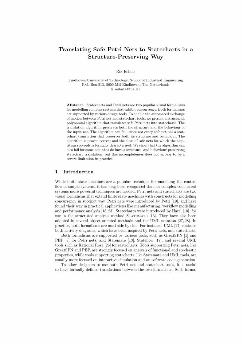
Fig. 1. Example Petri net
translations enable the automated exchange of models between different tools [8,9, 21]. For instance, a designer can first use a Petri net tool to analyse functionalproperties of a net design, next use an automated translation to transform thenet into a statechart, and then use a statechart tool to generate software code.
Ideally, such translations preserve the behaviour of the original model [9],neither reducing nor adding behaviour. Moreover, such translations should pre-serve the syntactic structure of the input models as much as possible, to supportroundtrip engineering and to make it easier for designers to understand the pro-duced translations. Without the requirement of structure preservation, for eachmodel with finite behavior a trivial translation exists: compute the transitionsystem of a model in formalism A, which resembles a finite state machine, andtranslate this transition system into formalism B. However, the syntactic struc-ture of the two models would then be completely different, as the input modelis concurrent but the output model sequential. Moreover, such a translation isprohibitively expensive for large models due to the state explosion problem.
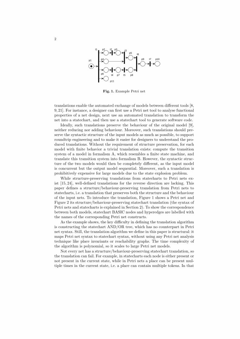
While structure-preserving translations from statecharts to Petri nets ex-ist [15, 24], well-defined translations for the reverse direction are lacking. Thispaper defines a structure/behaviour-preserving translation from Petri nets tostatecharts, i.e. a translation that preserves both the structure and the behaviourof the input nets. To introduce the translation, Figure 1 shows a Petri net andFigure 2 its structure/behaviour-preserving statechart translation (the syntax ofPetri nets and statecharts is explained in Section 2). To show the correspondencebetween both models, statechart BASIC nodes and hyperedges are labelled withthe names of the corresponding Petri net constructs.
As the example shows, the key difficulty in defining the translation algorithmis constructing the statechart AND/OR tree, which has no counterpart in Petrinet syntax. Still, the translation algorithm we define in this paper is structural: itmaps Petri net syntax to statechart syntax, without using any Petri net analysistechnique like place invariants or reachability graphs. The time complexity ofthe algorithm is polynomial, so it scales to large Petri net models.
Not every net has a structure/behaviour-preserving statechart translation, sothe translation can fail. For example, in statecharts each node is either present ornot present in the current state, while in Petri nets a place can be present mul-tiple times in the current state, i.e. a place can contain multiple tokens. In that
3
p6
p4
p2
p1
p7
p3
p5
p8
p9
t1
t5
p11
A1
A2
O1
O2
O3
O5
O4
O6
root
p1 A3
A2
O5
O3 O4
O6
p11
p5A1
O1 O2
p6 p7 p8
p2 p3 p4
t2t3
t4
t6
p10t7 p9 p10
A3
Fig. 2. Statechart translation and its AND/OR tree for the Petri net in Figure 1
t1
p1
p2
p3
p4
t1
p1
t2p2
p3
p4
t3
t2
t3
(a) (b)
Fig. 3. Two Petri nets that have no structure/behaviour-preserving statechart trans-lations
case, the place and the Petri net are called unsafe. Therefore, an unsafe Petrinet like Figure 3(a) has no structure/behaviour-preserving statechart transla-tion, since an unsafe place cannot map to one BASIC node. Still, by using abehaviour-preserving translation from unsafe nets to safe nets [2], also an unsafenet can be translated to a statechart using the translation algorithm defined thispaper.
However, there do exist safe Petri nets like Figure 3(b) that have no struc-ture/ behaviour-preserving statechart translation, as we explain in Section 6.There we also show that there are safe nets for which the algorithm does notconstruct a statechart even though a structure/behaviour-preserving statecharttranslation does exist. Since these statecharts are not constructible by the algo-rithm, the algorithm is incomplete. However, such statecharts are not likely to bedrawn in practice, so this does not seem to be a severe limitation. In Section 6,we also formally characterise the subclass of safe nets for which the algorithmreturns a statechart, so the algorithm is sound and complete for this class ofPetri nets.
To simplify the exposition, we do not consider transition labels for statechartsand Petri nets in this paper. This implies we use a generic, abstract statechartsemantics in which transitions are not triggered by events, but are taken whentheir input nodes are in the current state. The translation defined in this papercan provide the basis for more advanced translations which deal with events and
4
data, for example. Moreover, we do not consider weights on Petri net arcs, sincethese are only useful for unsafe nets.
The remainder of this paper is structured as follows. Section 2 provides back-ground on Petri nets and statecharts. Section 3 explains the basics of the trans-lation, including three reduction steps on Petri nets. Next, Section 4 definesa polynomial algorithm that realises the translation using the three reductionsteps. In Section 5, the algorithm is proven correct and its run-time complex-ity is analysed. Section 6 analyses the expressiveness of the translation, i.e., itformally characterises the class of input Petri nets for which the translation suc-ceeds and the class of statecharts that the translation outputs. We also analysethe completeness of the algorithm. Section 7 presents related work. Section 8winds up with conclusions and further work.
2 Background
We recall some definitions of transition systems, Petri nets and statecharts. Read-ers familiar with Petri nets and statecharts can skip this section. However, notethat the statechart definition differs slightly from the traditional one; details canbe found below. Formal definitions of Petri nets can be found, among others,in [18, 22]. For statecharts, formal definitions can be found, among others, in [6,14, 20].
2.1 Transition systems
The execution semantics of both Petri nets and statecharts map into transitionsystems. A transition system is a tuple (S, −→ , init) where S is a set of states,−→ ⊆ S × S the transition relation, and init ∈ S is the initial state.
To compare different transition systems, we use the notion of isomorphism.Let (S1, −→ 1, init1) and (S2, −→ 2, init2) be two transition systems. An isomor-phism is a bijective function f : S1−→S2 such that f(init1) = init2 and (x, y) ∈−→ 1 if and only if (f(x), f(y)) ∈ −→ 2. Two transition systems (S1, −→ 1, init1)and (S2, −→ 2, init2) are isomorphic if and only if they are related by an isomor-phism.
2.2 Petri nets
Syntax. A Petri net (place/transition net) is a tuple PN = (P, T, F, ι), whereP is a finite set of states, T is a finite set of transitions, P ∩ T 6= ∅, F ⊆(P × T ) ∪ (T × P ) is a finite set of arcs, the flow relation, and ι ∈ P is thestart place, to be explained later. Petri nets are visualised as bipartite graphs, inwhich circles represent places, bars represent transitions, and arrows representthe flow relation. Standard definitions of Petri nets also use weights on arcs, butsince weights are only useful for unsafe nets (to be defined later), we do notconsider these here.
5
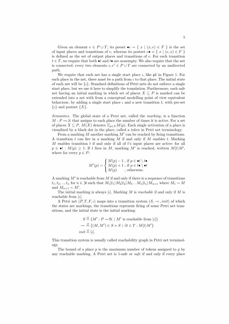
Given an element e ∈ P ∪ T , its preset •e = { x | (x, e) ∈ F } is the setof input places and transitions of e, whereas its postset e• = { x | (e, x) ∈ F }is defined as the set of output places and transitions of e. For each transitiont ∈ T , we require that both •t and t• are nonempty. We also require that the netis connected: every two elements e, e′ ∈ P ∪ T are connected by an undirectedpath.
We require that each net has a single start place ι, like p1 in Figure 1. Foreach place in the net, there must be a path from ι to that place. The initial stateof each net will be {ι}. Standard definitions of Petri nets do not enforce a singlestart place, but we use it here to simplify the translation. Furthermore, each safenet having an initial marking in which set of places X ⊆ P is marked can beextended into a net with from a conceptual modelling point of view equivalentbehaviour, by adding a single start place ι and a new transition tι with pre-set{ι} and postset {X}.
Semantics. The global state of a Petri net, called the marking , is a functionM : P −→N that assigns to each place the number of times it is active. For a setof places X ⊆ P , M(X) denotes Σp∈XM(p). Each single activation of a place isvisualised by a black dot in the place, called a token in Petri net terminology.
From a marking M another marking M ′ can be reached by firing transitions.A transition t can fire in a marking M if and only if M enables t. MarkingM enables transition t if and only if all of t’s input places are active: for allp ∈ •t : M(p) ≥ 1. If t fires in M , marking M ′ is reached, written M [t〉M ′,where for every p ∈ P :
M ′(p) =
M(p)− 1 , if p ∈ •t \ t•M(p) + 1 , if p ∈ t• \ •tM(p) , otherwise.
A marking M ′ is reachable from M if and only if there is a sequence of transitionst1, t2, . ., tn for n ∈ N such that M1[t1〉M2[t2〉M3 . . Mn[tn〉Mn+1 where M1 = Mand Mn+1 = M ′.
The initial marking is always [ι]. Marking M is reachable if and only if M isreachable from [ι].
A Petri net (P, T, F, ι) maps into a transition system (S, −→ , init) of whichthe states are markings, the transitions represent firing of some Petri net tran-sitions, and the initial state is the initial marking:
Sdf= {M ′ : P −→N | M ′ is reachable from [ι]}
−→ df= {(M,M ′) ∈ S × S | ∃t ∈ T : M [t〉M ′}init
df= [ι].
This transition system is usually called reachability graph in Petri net terminol-ogy.
The bound of a place p is the maximum number of tokens assigned to p byany reachable marking. A Petri net is 1-safe or safe if and only if every place
6
has bound of 1, i.e., no reachable marking M puts more than one token in someplace.
2.3 Statecharts
Statecharts extend finite state machines with AND/OR decomposition of statenodes and event broadcasting. As explained in the introduction, we do not focuson events, and therefore statechart transitions do not carry any label here.
The formal definition of the statechart syntax and semantics, presented be-low, differs somewhat from the original definition [6, 14, 20]. In particular, wedo not consider default nodes, since these do not have any counterpart in Petrinets and we consider normalised statechars, for which default nodes are super-fluous. Default nodes can always be eliminated from a statechart by applyingsome simple preprocessing [13]. This elimination results in a statechart with fullcompound transitions [13], which correspond to hyperedges whose targets areBASIC nodes. Since we omit default nodes, we have to phrase two requirementson hyperedges in the next section to ensure that when they are taken, the nextglobal state is a configuration.
Syntax. A statechart is a tuple (N,H, source, target, child, type, I), where
– N is a set of nodes,– H is a finite set of hyperedges, N ∩H = ∅,– source : H −→P(N) \ {∅} is a function defining the non-empty set of input
nodes for each hyperedge,– target : H −→P(N) \ {∅} is a function defining the non-empty set of output
nodes for each hyperedge,– child ⊆ N × N is a predicate that relates a node to its parent node, so
(n, n′) ∈ child means n is child of n′. A BASIC node has no children.– type : N −→{BASIC,AND, OR} is a function that assigns to each node its
type. We require type(x) = BASIC if and only if {y | (y, x) ∈ child} = ∅, soonly a non-BASIC node has children.
– I ⊆ N is the initial state (configuration), to be explained later.
BASIC nodes resemble places in a Petri net. Non-BASIC nodes are calledcomposite and are used to specify sequential (OR nodes) and concurrent be-haviour (AND nodes). Each composite node must have child nodes.
We denote by children(n) the set {n′ ∈ N | (n′, n) ∈ child}. Next, children ∗
denotes the reflexive-transitive closure of children, so children ∗(n) =⋃i≥0 childreni(n), where children0(n) = {n} and childreni+1(n) =⋃n′∈children(n) childreni(n′). If n′ ∈ children ∗(n), we say that n is ancestor of
n′ and n′ is descendant of n. Two nodes n, n′ are ancestrally related if either nis an ancestor of n′ or n′ an ancestor of n.
The child relation arranges the nodes in a tree with a root rt. Leaves are BA-SIC nodes. Each node n ∈ N , except rt, has one parent node, denoted parent(n).For technical reasons, root r is required to be an OR node.

7
Statecharts are visually represented as hierarchical hypergraphs [11]. We usethe UML statechart visualisation, so BASIC nodes are shown as rounded rect-angles and hyperedges with multiple source or multiple target nodes are shownas bars. The (OR) children of an AND node are separated by a dotted line. Thearrow leaving the black dot points at the initial node, which is explained later.The root node is never shown in a statechart diagram.
Semantics. Every global state of a statechart, called a configuration, must satisfyseveral constraints, defined below. First, we introduce some auxiliary definitions.The lowest common ancestor of a set X ⊆ N of nodes, written lca(X), is themost nested node n ∈ N that is an ancestor of every node in X:
X ⊆ children ∗(n)∀n′ ∈ N : X ⊆ children ∗(n′) ⇒ n ∈ children ∗(n′)
For example, in Figure 4, lca({n2, n3}) is OR node O1, whereas lca({n2, n5}) isAND node A.
Given a set X of nodes, lca+(X) is the most nested OR node that is ancestorof every node in X. For example, lca+({n4, n3}) = rt, since hidden root node rtis the OR parent of AND node A.
Two nodes n, n′ ∈ N are orthogonal if and only if they are not ancestrallyrelated and their lca is an AND node. In the example, nodes p2 and p5 areorthogonal, but nodes p2 and p6 are not (since their lowest common ancestor isOR node root rt).
A set X of nodes is consistent , written consistent(X), if and only if for everypair x, y ∈ X, either x and y are ancestrally related or x and y are orthogonal.For each hyperedge h, its source set and target set are required to be consistent,so consistent(source(h)) and consistent(target(h)).
A configuration is a maximal consistent set of nodes: adding a node to aconfiguration would make it inconsistent. In the example, among others {p1,rt}and {p2,p4,O1,O2,A,rt} are configurations. Configurations are the valid globalstates of a valid statechart.
A configuration C satisfies the following properties, for every x ∈ C:
– x ∈ ON ⇒ |children(x) ∩ C| = 1– x ∈ AN ⇒ children(x) ⊂ C– x 6= rt ⇒ parent(x) ∈ C.
A hyperedge h is enabled in configuration C if all its source nodes are in C,so source(h) ⊆ C. To define the effects of taking an enabled hyperedge, we needsome additional definitions. The scope of a hyperedge h is the most nested ORnode containing the sources and targets of h:
scope(h) df= lca+(source(h) ∪ target(h)).
Upon taking h, all strict descendants of scope(h) will be left. The next stateentered by taking h consists of the BASIC nodes in target(h), their ancestors,and nodes in the current configuration C that are ancestors of scope(h).

8
n4
n2
n1
n5
n3 n6
A
O1
O2
h1
h2
h3
h4
h5
Fig. 4. Non-normalised statechart
Next, the targets of h (and their ancestors below the scope of h) are added tothe state. If the resulting state is not a configuration, then target(h) is not com-plete. For instance, in Fig. 4, the target set of h4 is incomplete, since {n5,O2,A,rt}is not a configuration, as it contains AND node A, but not all children of A. Hareland Naamad [13] explain a static procedure for normalising statecharts, in whicheach incomplete target set X of a hyperedge is extended into a complete targetset. The resulting hyperedges with complete target sets are called full compoundtransitions [13]. A complete description of the procedure is out of scope here,but an important element is the use of the default child node (pointed to by anarrow leaving a black dot) for each OR node that causes incompletion of X.
Formally, a set X of BASIC nodes is complete, written complete(X), if andonly if adding a BASIC node to X yields an inconsistent set of nodes:
complete(X) ⇔ ∀n ∈ N : type(n) = BASIC ∧n 6∈ X ⇒ ¬consistent(X ∪{n}).
We require that complete(target(h)).Our translation maps Petri nets to normalised statecharts, such as the one
in Figure 2. Note that a normalised statechart is like an ordinary statechart,except that default nodes are superfluous, since each hyperedge has a completetarget set. Therefore, we omit default nodes from the statechart definition.
Upon taking hyperedge h, the configuration C changes into C ′, writtenC[h〉C ′, where
C ′ = dcomp((C \ children+(scope(h))) ∪ target(h))
where given a set S, the default completion dcomp(S) is the smallest set D suchthat
– S ⊆ D
– if s ∈ D and s 6= r then parent(s) ∈ D.
If h has a complete target set, then C ′ is a configuration.Given a statechart SC in which every hyperedge has a complete target set,
configuration C is reachable if and only if there is a sequence of hyperedgesleading from the initial configuration I to C. A wellformed statechart maps into
9
a transition system (S, −→ , init), where
Sdf= { C ⊆ N | C is a configuration and reachable }
−→ df= {(C, C ′) ∈ S × S | ∃h ∈ H : C[h〉C ′}init
df= I.
3 Translation Basics
In this section, we explain the basics of the translation algorithm defined in thenext section.
Preserving structure. To ensure that the constructed translation is structure-preserving, the algorithm maps each place to a BASIC node and each transitiont with preset X and postset Y to a hyperedge h having source set X and targetset Y . Both mappings are bijective. Thus, the translation algorithm embeds thePetri net structure in the statechart structure.
Technically, a translation PNtoSC from Petri nets to statecharts is structurepreserving if and only if for each Petri net (P, T, F, ι) that translates to statechart((N, H, source, target, child, type, I), there are bijective functions f : P −→BNand g : T −→H, where BN = {n ∈ N |type(n) = BASIC} such that for each p ∈P and t ∈ T , (p, t) ∈ F ⇔ f(p) ∈ source(g(t)), (t, p) ∈ F ⇔ f(p) ∈ target(g(t)),and p = ι ⇔ f(p) ∈ I. Thus, a structure-preserving translation embeds a Petrinet structure into a statechart structure.
To simplify the definitions of the translations, we will use the identity functionfor functions f and g. So each place p will map to a BASIC node p and eachtransition t to a hyperedge t.
Building the AND/OR tree. The AND/OR nodes of the statechart have no coun-terpart in the Petri net, but are constructed by the translation algorithm. Thesenodes have to be arranged in a tree, the leafs of which are the BASIC nodes.To construct the internal nodes of the tree, of type AND and OR, transitionsare processed. For each transition t, an OR node o must be created which actsas the scope of hyperedge t in the statechart. Moreover, if t has a non-singletonpreset (postset), then the places in the preset (postset) are active in parallel,so an AND node, child of o, needs to be constructed that contains all BASICnodes in •t (t•). For example, for transition t3 in Figure 1, in the correspondingstatechart in Figure 2 AND node A1 has been created.
Nesting nodes. Complicating issue is that an AND node can be nested insideanother AND node. For example, in Figure 2, AND node A1 is nested insideA2 and A3. Thus, the translation algorithm cannot create for the postset of t1an AND node a with four OR children that have the output places of t1 asBASIC children; instead, it needs to create an AND node with two OR children,in one of which AND nodes A2 and A1 are nested. To create a proper nesting,we construct the AND/OR tree bottom-up. So, when creating the AND/OR

10
t1 t2 t3
o1
o2 o3
o4
o5
o6 o7 o8
o9 o10
o11
t4 t5
t6
t7
o2 o4
p2 p3 p4
o1
p1
o5
p5
o6
p6
o7
p7 p8
o9
p9 p10
o3 o8 o10
p11
o11
Fig. 5. Initial Petri net and initially constructed AND/OR trees for Figure 1
tree for the Petri net in Figure 1, first AND node A1 and its OR children isconstructed, then A2 and its OR children, and finally A3 and its OR children.
Ordering of transitions. To ensure that the tree is constructed bottom-up, tran-sitions need to be processed in a certain order. For example, we see that inFigure 2 the scope of hyperedge t2 (OR node O1) is more nested than that oft1 (root rt). Therefore, the transition t2 needs to be processed before t1.
The ordering constraint we use is that a transition t1 should be processedbefore a transition t2, written t1 ≺ t2, if either •t1 ⊂ t2• or t1• ⊂ •t2. In bothcases, in the resulting statechart the scope of hyperedge t1 is nested inside thescope of t2. Therefore t1 needs to be processed before t2. A transition t can onlybe processed if there exists no other transition t′ such that t′ ≺ t.
Processing of transitions. Conceptually, the actual construction of the AND/ORtree is done by letting each place link to a partial AND/OR tree that has an ORroot. A transition is processed by reducing it, as well as its preset and postset, toa single place. The AND/OR tree of this new place is constructed by aggregatingthe AND/OR trees of the places in the pre- and postset of t.
To simplify the presentation, we let each place be the root of the correspond-ing tree, rather than annotating a place with a tree. Initially, for each place p acorresponding tree, consisting of OR root op and its child p is constructed. Placeop replaces p in the original input net. Figure 5 shows for the example Petri netin Figure 1 the initial net and the initially constructed AND/OR trees.
Next, we explain the reduction steps, in which the AND/OR trees get merged,in detail.
Reduction step 1. The first reduction step consists of two substeps that aresymmetrical, one reducing the preset of a transition, the other its postset. Instep 1a, the non-singleton preset Q = {q1, . ., qn} of transition t is reduced to aplace p that becomes the single input place of t. If t already has a singe inputplace, step 1a is skipped. Otherwise, each transition in T that has a place inQ as input or output place, instead gets p as input or output place. If such aneighbouring transition has multiple places in Q in its preset or postset, theseare all removed and replaced by single place p. The AND/OR tree for p is
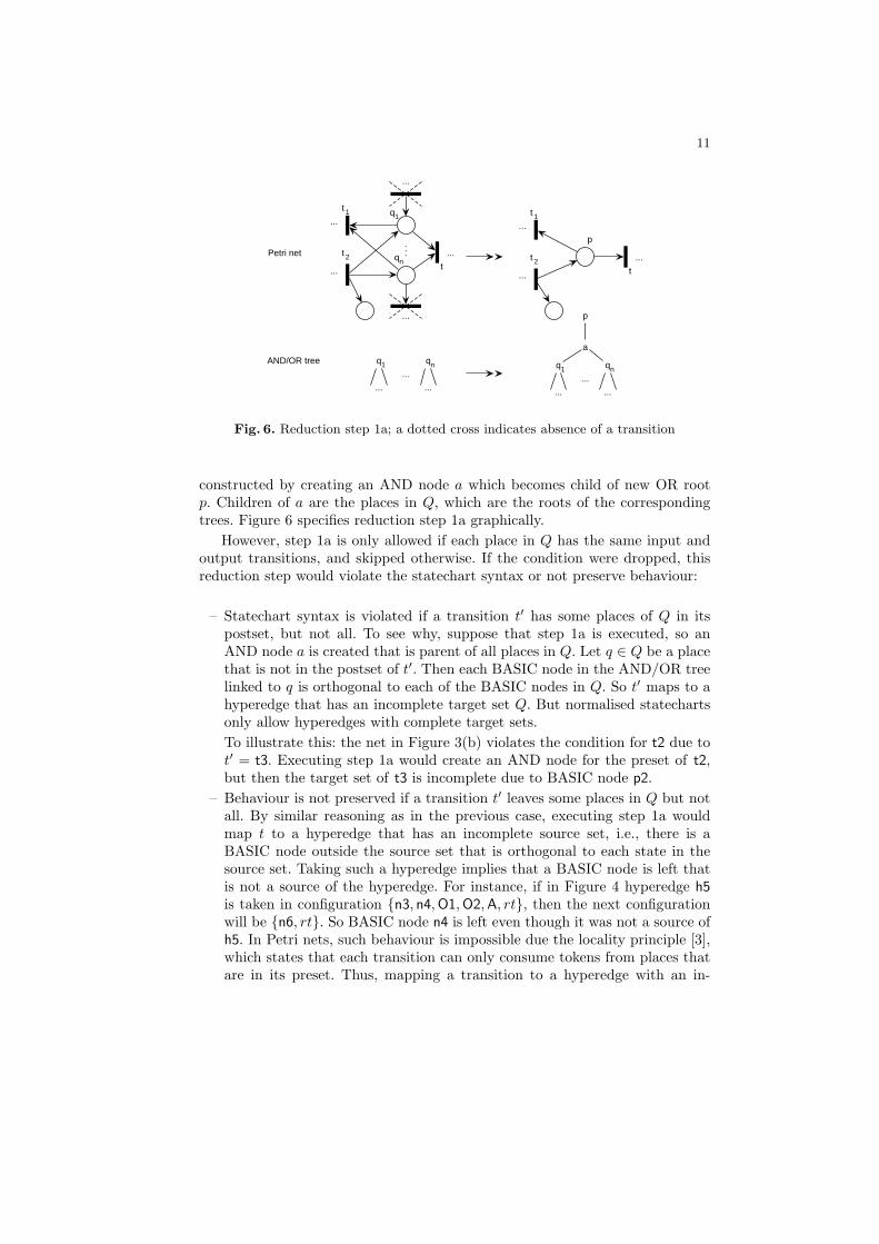
11
p
q1
...
qn
...
tqn
q1
t 2
t 1
...Petri net
AND/OR tree
...
...
...
...
... t
t 2
t 1
...
...
...
...q1
...
qn
...
...
a
p
Fig. 6. Reduction step 1a; a dotted cross indicates absence of a transition
constructed by creating an AND node a which becomes child of new OR rootp. Children of a are the places in Q, which are the roots of the correspondingtrees. Figure 6 specifies reduction step 1a graphically.
However, step 1a is only allowed if each place in Q has the same input andoutput transitions, and skipped otherwise. If the condition were dropped, thisreduction step would violate the statechart syntax or not preserve behaviour:
– Statechart syntax is violated if a transition t′ has some places of Q in itspostset, but not all. To see why, suppose that step 1a is executed, so anAND node a is created that is parent of all places in Q. Let q ∈ Q be a placethat is not in the postset of t′. Then each BASIC node in the AND/OR treelinked to q is orthogonal to each of the BASIC nodes in Q. So t′ maps to ahyperedge that has an incomplete target set Q. But normalised statechartsonly allow hyperedges with complete target sets.To illustrate this: the net in Figure 3(b) violates the condition for t2 due tot′ = t3. Executing step 1a would create an AND node for the preset of t2,but then the target set of t3 is incomplete due to BASIC node p2.
– Behaviour is not preserved if a transition t′ leaves some places in Q but notall. By similar reasoning as in the previous case, executing step 1a wouldmap t to a hyperedge that has an incomplete source set, i.e., there is aBASIC node outside the source set that is orthogonal to each state in thesource set. Taking such a hyperedge implies that a BASIC node is left thatis not a source of the hyperedge. For instance, if in Figure 4 hyperedge h5is taken in configuration {n3, n4,O1, O2, A, rt}, then the next configurationwill be {n6, rt}. So BASIC node n4 is left even though it was not a source ofh5. In Petri nets, such behaviour is impossible due the locality principle [3],which states that each transition can only consume tokens from places thatare in its preset. Thus, mapping a transition to a hyperedge with an in-
12
t1
t3
o1
o2,3
o4
o5
o6 o7,8
o9,10
o11
t4
t6
o2,3 o4
p2 p3 p4
o1
p1
o5
p5
o6
p6
o7,8
p7 p8
o9,10
p9 p10
o11
p11
t1 t3
o1
o2,3,4 o5
o6 o7,8
o9,10
o11
t4
t6
o2,3 o4
p2 p3 p4
o1
p1
o5
p5
o6
p6
o7,8
p7 p8
o9,10
p9 p10
o2,3,4
a2,3,4
o11
p11
reduction step 1a
for t3
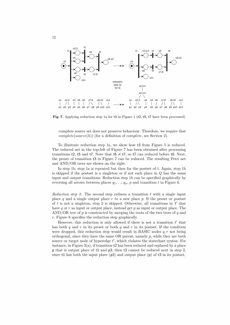
Fig. 7. Applying reduction step 1a for t3 in Figure 1 (t2, t5, t7 have been processed)
complete source set does not preserve behaviour. Therefore, we require thatcomplete(source(h)) (for a definition of complete, see Section 2).
To illustrate reduction step 1a, we show how t3 from Figure 5 is reduced.The reduced net in the top-left of Figure 7 has been obtained after processingtransitions t2, t5 and t7. Note that t6 6≺ t7, so t7 can reduced before t6. Next,the preset of transition t3 in Figure 7 can be reduced. The resulting Petri netand AND/OR trees are shown on the right.
In step 1b, step 1a is repeated but then for the postset of t. Again, step 1bis skipped if the postset is a singleton or if not each place in Q has the sameinput and output transitions. Reduction step 1b can be specified graphically byreversing all arrows between places q1, . ., qn, p and transition t in Figure 6.
Reduction step 2. The second step reduces a transition t with a single inputplace q and a single output place r to a new place p. If the preset or postsetof t is not a singleton, step 2 is skipped. Otherwise, all transitions in T thathave q or r as input or output place, instead get p as input or output place. TheAND/OR tree of p is constructed by merging the roots of the two trees of q andr. Figure 8 specifies the reduction step graphically.
However, this reduction is only allowed if there is not a transition t′ thathas both q and r in its preset or both q and r in its postset. If the conditionwere dropped, this reduction step would result in BASIC nodes q, r not beingorthogonal, since they have the same OR parent, namely p, while they are bothsource or target node of hyperedge t′, which violates the statechart syntax. Forinstance, in Figure 3(a), if transition t2 has been reduced and replaced by a placep that is output place of t1 and p3, then t3 cannot be reduced next in step 2,since t1 has both the input place (p3) and output place (p) of t3 in its postset.

13
q r
t
q
q qk1
...
r
r rl1
...
t 1 t 2
t 3 t 4
p
t 1 t 2
t 3 t 4
p
q qk1
... r rl1
...
...
... ... ... ...
... ......
Petri net
AND/OR tree
Fig. 8. Reduction step 2; a dotted cross indicates absence of a transition
t1t3
o1
o2,3,4 o5
o6 o7,8
o9,10
o11
t4
t6
o2,3 o4
p2 p3 p4
o1
p1
o5
p5
o6
p6
o7,8
p7 p8
o9,10
p9 p10
o2,3,4
a2,3,4
o11
p11
reduction step 2 for t3
t1
o1
o2,3,4,5
o6 o7,8
o9,10
o11
t4
t6
o2,3 o4
p2 p3 p4
o1
p1 p5
o6
p6
o7,8
p7 p8
o9,10
p9 p10
o2,3,4,5
a2,3,4
o11
p11
Fig. 9. Applying reduction step 2 for t3 in Figure 1
Continuing with the processing of t3, the reduced net on the righthand sidein Figure 7 can be further reduced since t3 has a single input place o2,3,4 and asingle output place o5. Figure 9 shows the resulting net and the node hierarchies.
Failure. If one the steps cannot be applied since its condition is not met, thenthe translation fails. In some peculiar cases, a structure/behaviour-preservingstatechart may exist. We discuss this issue in detail in Section 6.
4 Algorithm
We now explain the actual translation algorithm PetriNetToStatechart indetail. The algorithm expects as input a Petri net (P, T, F, ι) and returns a stat-echart. If the translation fails, the returned statechart is empty. The algorithmhas been implemented in a prototype tool that reads PNML, an XML-format
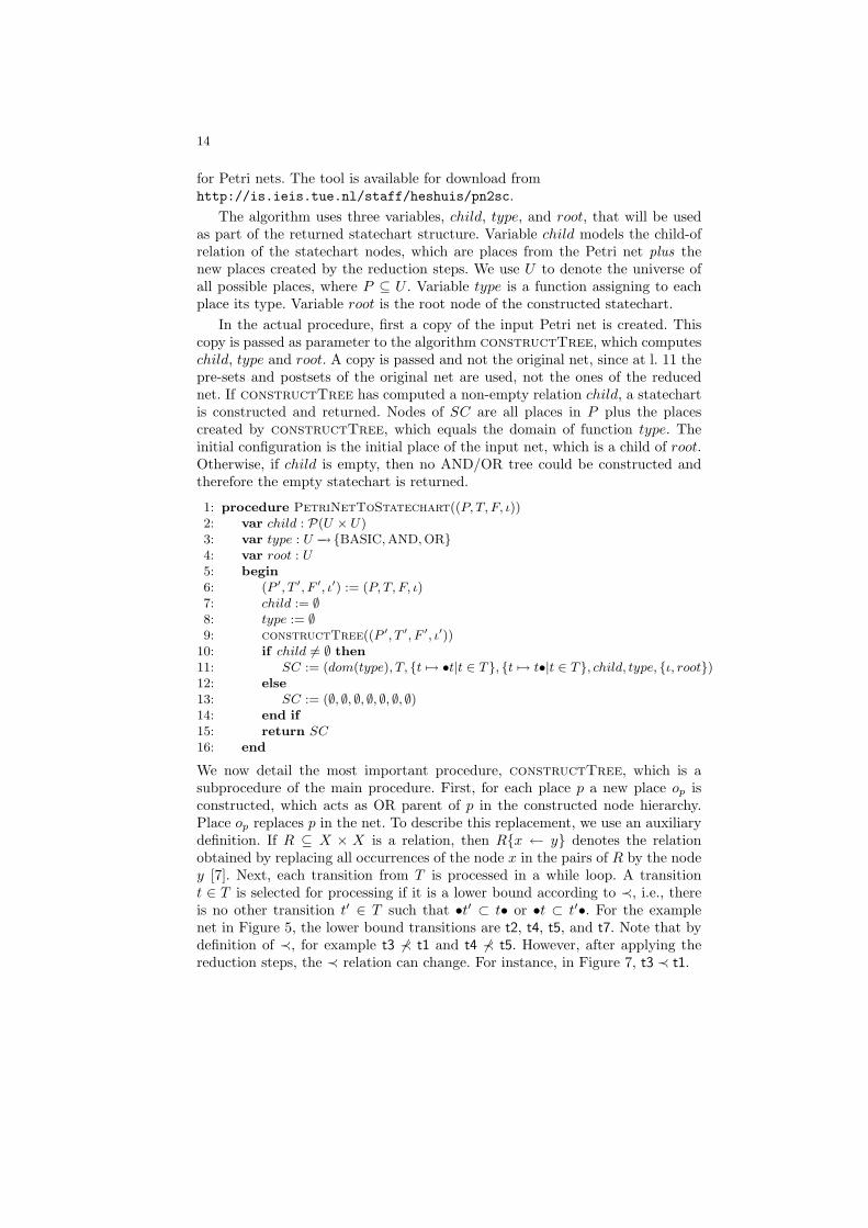
14
for Petri nets. The tool is available for download fromhttp://is.ieis.tue.nl/staff/heshuis/pn2sc.
The algorithm uses three variables, child, type, and root, that will be usedas part of the returned statechart structure. Variable child models the child-ofrelation of the statechart nodes, which are places from the Petri net plus thenew places created by the reduction steps. We use U to denote the universe ofall possible places, where P ⊆ U . Variable type is a function assigning to eachplace its type. Variable root is the root node of the constructed statechart.
In the actual procedure, first a copy of the input Petri net is created. Thiscopy is passed as parameter to the algorithm constructTree, which computeschild, type and root. A copy is passed and not the original net, since at l. 11 thepre-sets and postsets of the original net are used, not the ones of the reducednet. If constructTree has computed a non-empty relation child, a statechartis constructed and returned. Nodes of SC are all places in P plus the placescreated by constructTree, which equals the domain of function type. Theinitial configuration is the initial place of the input net, which is a child of root.Otherwise, if child is empty, then no AND/OR tree could be constructed andtherefore the empty statechart is returned.
1: procedure PetriNetToStatechart((P, T, F, ι))2: var child : P(U × U)3: var type : U −→{BASIC, AND, OR}4: var root : U5: begin6: (P ′, T ′, F ′, ι′) := (P, T, F, ι)7: child := ∅8: type := ∅9: constructTree((P ′, T ′, F ′, ι′))
10: if child 6= ∅ then11: SC := (dom(type), T, {t 7→ •t|t ∈ T}, {t 7→ t•|t ∈ T}, child, type, {ι, root})12: else13: SC := (∅, ∅, ∅, ∅, ∅, ∅, ∅)14: end if15: return SC16: end
We now detail the most important procedure, constructTree, which is asubprocedure of the main procedure. First, for each place p a new place op isconstructed, which acts as OR parent of p in the constructed node hierarchy.Place op replaces p in the net. To describe this replacement, we use an auxiliarydefinition. If R ⊆ X × X is a relation, then R{x ← y} denotes the relationobtained by replacing all occurrences of the node x in the pairs of R by the nodey [7]. Next, each transition from T is processed in a while loop. A transitiont ∈ T is selected for processing if it is a lower bound according to ≺, i.e., thereis no other transition t′ ∈ T such that •t′ ⊂ t• or •t ⊂ t′•. For the examplenet in Figure 5, the lower bound transitions are t2, t4, t5, and t7. Note that bydefinition of ≺, for example t3 6≺ t1 and t4 6≺ t5. However, after applying thereduction steps, the ≺ relation can change. For instance, in Figure 7, t3 ≺ t1.
15
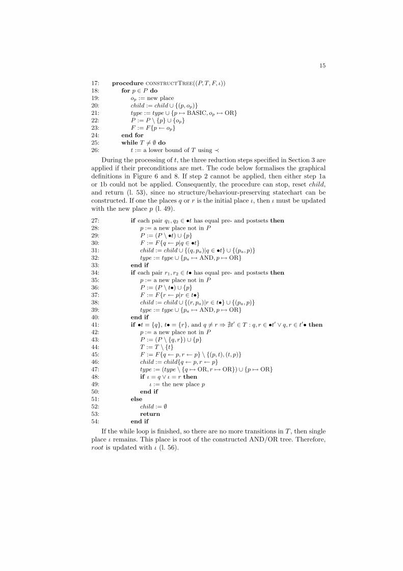
17: procedure constructTree((P, T, F, ι))18: for p ∈ P do19: op := new place20: child := child ∪ {(p, op)}21: type := type ∪ {p 7→ BASIC, op 7→ OR}22: P := P \ {p} ∪ {op}23: F := F{p ← op}24: end for25: while T 6= ∅ do26: t := a lower bound of T using ≺
During the processing of t, the three reduction steps specified in Section 3 areapplied if their preconditions are met. The code below formalises the graphicaldefinitions in Figure 6 and 8. If step 2 cannot be applied, then either step 1aor 1b could not be applied. Consequently, the procedure can stop, reset child,and return (l. 53), since no structure/behaviour-preserving statechart can beconstructed. If one the places q or r is the initial place ι, then ι must be updatedwith the new place p (l. 49).
27: if each pair q1, q2 ∈ •t has equal pre- and postsets then28: p := a new place not in P29: P := (P \ •t) ∪ {p}30: F := F{q ← p|q ∈ •t}31: child := child ∪ {(q, pa)|q ∈ •t} ∪ {(pa, p)}32: type := type ∪ {pa 7→ AND, p 7→ OR}33: end if34: if each pair r1, r2 ∈ t• has equal pre- and postsets then35: p := a new place not in P36: P := (P \ t•) ∪ {p}37: F := F{r ← p|r ∈ t•}38: child := child ∪ {(r, pa)|r ∈ t•} ∪ {(pa, p)}39: type := type ∪ {pa 7→ AND, p 7→ OR}40: end if41: if •t = {q}, t• = {r}, and q 6= r ⇒ @t′ ∈ T : q, r ∈ •t′ ∨ q, r ∈ t′• then42: p := a new place not in P43: P := (P \ {q, r}) ∪ {p}44: T := T \ {t}45: F := F{q ← p, r ← p} \ {(p, t), (t, p)}46: child := child{q ← p, r ← p}47: type := (type \ {q 7→ OR, r 7→ OR}) ∪ {p 7→ OR}48: if ι = q ∨ ι = r then49: ι := the new place p50: end if51: else52: child := ∅53: return54: end if
If the while loop is finished, so there are no more transitions in T , then singleplace ι remains. This place is root of the constructed AND/OR tree. Therefore,root is updated with ι (l. 56).
16
55: end while56: root := ι57: end procedure58: end procedure
5 Correctness and Complexity
We prove the correctness and analyse the run-time complexity of the algorithm.
Correctness. We prove the correctness of the algorithm in several steps. First, weprove that wellformed statecharts, i.e. statecharts in which every hyperedge hasa complete source set, translates in a structure-preserving way to a Petri net thathas isomorphic behaviour. Next, we use this result to prove that the translationalgorithm yields a wellformed statechart that has behaviour isomorphic to thebehaviour of the input net. Thus, the translation is behaviour-preserving.
A statechart (N,H, source, target, child, type, I) is wellformed if for each h ∈H, complete(source(h)). Recall from statechart syntax, that by default eachhyperedge h satisfies complete(target(h)), consistent(source(h)) andconsistent(target(h)).
Below we prove that structure-preserving translations are correct for well-formed statecharts. First we need to introduce an auxiliary definition and theo-rem. Each wellformed statechart can be translated into a (structure-preserving)Petri net using function SCtoPN :
SCtoPN((N,H, source, target, child, type, I) = (P, T, F, ι)
where
– Pdf= BN
– Tdf= H
– Fdf= { (n, h) | n ∈ BN ∩ source(h) } ∪ { (h, n) | n ∈ BN ∩ target(h) }
– ιdf= the single element in I ∩BN .
where BN = { n ∈ N | type(n) = BASIC }.The next theorem shows that the transition systems of a wellformed state-
chart and its underlying net are isomorphic.
Theorem 1. Let SC be a wellformed statechart. The transition system ofSCtoPN(SC) is isomorphic to the transition system of SC.
Proof. We define a bijective function f that maps each state Ci ⊆ N of thetransition system of SC to a state Mi : P −→{0, 1} of the transition system ofPN :
f(Ci) = {n 7→ 1 | n ∈ Ci ∩BN} ∪ {n 7→ 0 | n ∈ BN \ Ci}.Clearly, f(I) = M . Next, we need to prove condition (C, C ′) ∈ −→ SC if
and only if (f(C), f(C ′) ∈ −→ PN , where −→ SC and −→ PN are the transitionrelations of the transition systems of SC and SCtoPN(SC), respectively. Thiscan be proven since C[h〉C ′ ⇔ f(C)[h〉f(C ′), which follows easily from thedefinition of wellformedness. ut
17
Using Theorem 1, we show that structure-preserving translations are correctfor wellformed statecharts: if such a translation yields a wellformed statechart,the input Petri net and statechart have isomorphic transition systems.
Theorem 2. Let PNtoSC be a structure-preserving translation from Petri netsto statecharts and let PN be a Petri net that PNtoSC maps to a wellformedstatechart SC. Then the transition system of SC is isomorphic to that of PN .
Proof. Since PNtoSC is structure preserving and from the definition of SCtoPN ,it follows that SCtoPN(SC) is a Petri net isomorphic to PN . Hence, the tran-sition systems of PN and SCtoPN(SC) are isomorphic too. The result thenfollows immediately from Theorem 1. ut
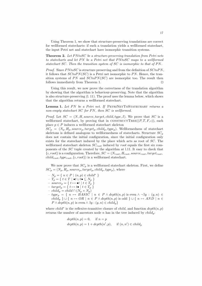
Using this result, we now prove the correctness of the translation algorithmby showing that the algorithm is behaviour-preserving. Note that the algorithmis also structure-preserving (l. 11). The proof uses the lemma below, which showsthat the algorithm returns a wellformed statechart.
Lemma 1. Let PN be a Petri net. If PetriNetToStatechart returns anon-empty statechart SC for PN , then SC is wellformed.
Proof. Let SC = (N, H, source, target, child, type, I). We prove that SC is awellformed statechart, by proving that in constructTree((P, T, F, ι)), eachplace p ∈ P induces a wellformed statechart skeletonSCp = (Np,Hp, sourcep, targetp, childp, typep). Wellformedness of statechartskeletons is defined analogous to wellformedness of statecharts. Structure SCp
does not contain the initial configuration, since the initial configuration onlyexists for the statechart induced by the place which acts as root of SC. Thewellformed statechart skeleton SCroot induced by root equals the first six com-ponents of the SC tuple created by the algorithm at l.11. It easy to check that{ι, root} is a configuration. Therefore, SC = (Nroot,Hroot, sourceroot, targetroot,childroot, typeroot, {ι, root}) is a wellformed statechart.
We now prove that SCp is a wellformed statechart skeleton. First, we defineSCp = (Np,Hp, sourcep, targetp, childp, typep), where
– Np = { n ∈ P | (n, p) ∈ child∗ }– Tp = { t ∈ T | •t ∪ t• ⊆ Np }– sourcep = { t 7→ •t | t ∈ Tp }– targetp = { t 7→ t• | t ∈ Tp }– childp = child ∩ (Np ×Np)– typep = { n 7→ BASIC | n ∈ P ∧ depth(n, p) is even ∧ ¬∃y : (y, n) ∈
childp } ∪ { n 7→ OR | n ∈ P ∧ depth(n, p) is odd } ∪ { n 7→ AND | n ∈P ∧ depth(n, p) is even ∧ ∃y : (y, n) ∈ childp}
where child∗ is the reflexive-transitive closure of child, and function depth(n, p)returns the number of ancestors node n has in the tree induced by childp:
depth(n, p) = 0, if n = p
depth(n, p) = 1 + depth(n′, p), if (n, n′) ∈ childp
18
By definition of Np and childp, for each n ∈ Np, either n = p or there exists aunique n′ ∈ Np such that (n, n′) ∈ childp.
We prove that SCp is a wellformed statechart skeleton by induction on thenumber of iterations of the while-loop started at l.25. The induction hypothesis isthat each place p induces a wellformed statechart skeleton SCp and two differentplaces p1, p2 ∈ P induce statechart skeletons with disjoint node sets, so Np1 ∩Np2 = ∅.
Base step. After l.24, each place p induces a statechart skeleton SCp withno hyperedges and with root p, which has a single child. Clearly, SCp is a state-chart skeleton. Moreover, by construction (l.20-l.21) two different places inducestatechart skeletons with disjoint node sets.
Induction step. Let X be the set of places that are removed from (P, T, F, ι)in one of the three reduction steps in the current iteration of the while loop(l.25), and let p be the new place that replaces the places in X. Let SCp be thestatechart skeleton that is induced by p. We show that (i) its nodes are arrangedin an AND/OR tree, and (ii) its hyperedges have consistent and complete sourcesets and consistent and complete target sets.
(i) It is easy to check, using the update of child (l.31, l.38, l.46), that p inducesa statechart skeleton whose nodes are arranged in an AND/OR tree, using theproperty (from the induction hypothesis) that for each pair of nodes x1, x2 ∈ X,the nodes of the statechart skeletons induced by x1 and x2 are disjoint.
(ii) Let t ∈ T be transition such that t ∈ Hp but t 6∈ Hx for any x ∈ X. So thas as scope p. (By the induction hypothesis, all hyperedges in Hx, for x ∈ X,have consistent and complete source and target sets.) We have to show that thas a consistent and complete source set and a consistent and complete targetset. Let S be a source set or target set of h.
– Regarding completeness, observe that S is incomplete if there is a BASICnode orthogonal to each of the nodes in S. But the conditions on reductionstep 1a and 1b prevent this from happening. Thus S is complete.
– Regarding consistency, two BASIC nodes in S can only get a least commonancestor of type OR by reduction step 2. The precondition for step 2 ensuresthat such BASIC nodes are not related by any AND node (created in steps1a and 1b). Thus, S is consistent.
Therefore, each place p induces a wellformed statechart skeleton SCp. utTheorem 3. Let PN be a Petri net. If PetriNetToStatechart returns anon-empty statechart SC for PN , then the transition systems of PN and SCare isomorphic.
Proof. By Lemma 1, SC is wellformed. Next, since SC is wellformed, by Theo-rem 2 the transition systems of PN and SC are isomorphic. ut
Complexity. The worst-case time complexity of the algorithm is polynomial inthe size of the input Petri net PN = (P, T, F, ι). The while-loop is executed |T |times in the worst case. Next, finding a lower bound transition t from T at l. 26

19
takes |P | + |T | time. Thus, the worst-case time complexity of the algorithm isO(|T | · (|P |+ |T |)), so polynomial in the size of PN .
6 Expressiveness
We analyse the expressiveness of the translation, both from the input side andthe output side. Next, we analyse the completeness of the translation algorithm.We end with an example of an unstructured net that the translation maps to anon-empty statechart.
Input side. To characterise the class of nets that the algorithm maps to non-empty statecharts, we first need the auxiliary notion of an area, which is a newconcept in Petri net theory. Let PN = (P, T, F, ι) be a Petri net and X ⊆ Pbe a nonempty set of places. Then X is an area if and only if for every t ∈ T ,•t ⊆ X ⇔ t• ⊆ X. For example, in Figure 1, sets {p2, p3} and {p2, p3, p4, p5} areareas. Given a set of places X ⊆ P , the minimal area of X, denoted minArea(X),is the minimal set of places Y ⊆ P such that X ⊆ Y and Y is an area. Forexample, minArea({p3, p4}) = {p2, p3, p4, p5}.
We use the notion of area to define the notion of cover. Let X be the preset orpostset of some transition t. Then the cover of X, written cover(X) is defined tobe
⋃x∈X minArea({x}). If the translation succeeds, then the AND node created
for X contains all places in cover(X) as BASIC nodes. For example, in Figure 1,cover({p3, p4}) = {p2, p3, p4}. The places in this set are BASIC descendants ofA1 in Figure 2. Note that p5 is not included in cover({p3, p4}).
A Petri net PN has nestable covers if and only if for every X,Y ⊆ P such thatX and Y are preset or postset of some transitions in T , cover(X)∩cover(Y ) 6= ∅implies cover(X) ⊆ cover(Y ) or cover(Y ) ⊆ cover(X). The net in Figure 11 doesnot have nestable covers, since cover(t2•) and cover(•t5) are not nestable. Butboth unsafe nets in Figure 3 do have nestable covers, so we need an additionalcriterion to rule out those nets.
A transition t has consistent areas if and only if for every set X,Y ⊆ P suchthat X∪Y ⊆ •t or X∪Y ⊆ t•, if X∩Y = ∅ then minArea(X)∩minArea(Y ) = ∅.A Petri net PN has consistent areas if each transition has consistent areas. Thenets in Figure 3 do not have consistent areas: in both nets, minArea({p2}) ∩minArea({p3}) 6= ∅. In Figure 3(b), minArea({p3}) = {p1, p2, p3, p4}.
The algorithm returns a non-empty statechart if and only if the input Petrinet has nestable covers and consistent areas. Before we present the theorem andits proof, we introduce some lemmas that we use in the proof.
Lemma 2. After reducing a transition t in constructTree, the reduced nethas nestable covers and consistent areas if and only if the original net hasnestable covers and consistent areas.
Proof. ⇒: Suppose the reduced net has nestable covers and consistent areas. Atransition can only be reduced under certain preconditions. The preconditionsfor non-singleton pre- and postsets (step 1a and 1b) guarantee that the covers

20
of the pre- and postsets of the transitions incident to the input and outputplaces of t are nestable. The precondition for singleton pre- and postsets (step2) guarantees that there is no transition t′ such that t′ does not have consistentareas. So the original net has nestable covers and consistent areas.
⇐: Suppose the original net has nestable covers and consistent areas. If t isreduced, then t and its pre- and postset are replaced by a single place. Thus,each area X in the original net that contains cover(Y ) as subset, where Y = •tor Y = t•, corresponds to an area X \ cover(Y ) ∪ {p} in the reduced net. It iseasy to check that also in the reduced net, the covers are nestable and the areasare consistent. ut
Lemma 3. If a Petri net can be reduced in an iteration in constructTree,it has nestable covers and consistent areas.
Proof. The Petri net with a single place and no transitions has nestable coversand consistent areas. By Lemma 2, in each iteration the net that is reduced alsohas nestable covers and consistent areas. Therefore PN has nestable covers andconsistent areas. ut
Lemma 4. If a transition t cannot be reduced by constructTree, i.e., line 53is reached, then either there is a pair of transitions t1, t2 ∈ T having pre- orpostsets X1, X2, so Xi = •ti or Xi = ti•, for i ∈ {1, 2}, such that their covers,cover(X1) and cover(X2), are not nestable, or there is a transition t that hasno consistent areas.
Proof. Observe that by Lemma 2, reducing a net preserves nestability of coversand consistency of areas. Thus, we can prove that the reduced net has unnestablecovers or a transition that has no consistent areas. There are three cases: (i) thas a non-singleton preset, so the algorithm failed at reduction step 1a, (ii) t hasa non-singleton postset, so the algorithm failed at reduction step 1b, or (iii) t hasa singleton preset and a singleton postset, so the algorithm failed at reductionstep 2. Since cases (i) and (ii) are symmeterical, we only consider (i) and (iii).
(i) t has a non-singleton preset and the condition of step 1a for t is violated.Then the condition of step 1 is violated, so there are places p1, p2 ∈ •t such that•p1 6= •p2 or p1• 6= p2•. We only consider the case •p1 6= •p2, the other case is bysymmetrical reasoning. Either there is a transition t1 ∈ •p1 \ •p2, or a transitiont2 ∈ •p2 \ •p1, or a transition t3 ∈ p1• \ p2•, or a transition t4 ∈ p2• \ p1•. Weonly consider the first option, the others are by symmetrical reasoning. If t1 = t,then minArea(p1) = minArea(t), so then t has no consistent areas.
Otherwise, t1 6= t; see Figure 10. Note that p1 ∈ cover(t1•)∩ cover(•t). Sincet1 6≺ t, we have t1• 6⊂ •t. Thus, t1 has an output place p such that p 6∈ •t. IfminArea(p) = minArea(p2), then there is a transition tp2 such that tp2• = {p2}or •tp2 = {p2}. In both cases, tp2 ≺ t, which contradicts that t is the lower boundtransition w.r.t. ≺. So minArea(p) 6= minArea(p2). Therefore, cover(•t) 6⊆cover(t1•) and cover(•t) 6⊇ cover(t1•). Hence, cover(•t) and cover(t1•) are notnestable. Thus the net does not have nestable covers.
21
t1
p2
p1 t
p
...
... ...
Fig. 10. Petri net structure used in proof of Lemma 4
(iii) t has a singleton preset and singleton postset and the condition forstep 2 is violated. Let •t = {q} and t• = {r}, where q 6= r. Then there is atransition t′ such that q, r ∈ •t′ or q, r ∈ t′•. Since q 6= r, {q} and {r} aredisjoint. But due to t, q and r are both in minArea({q}) and minArea({r}), sominArea({q}) ∩minArea({r}) 6= ∅. Thus, t has no consistent areas.
Thus, in all three cases (i), (ii), (iii), either transition t has no consistentareas or the net has unnestable covers. ut
Using these lemmas, we now prove the main theorem.
Theorem 4. Let PN be a Petri net. Algorithm PetriNetToStatechart re-turns a non-empty statechart SC for PN if and only if PN has nestable coversand consistent areas.
Proof. ⇒: Follows immediately from Lemma 3.⇐: Follows immediately from Lemma 4. utTheorem 4 formally characterises Petri nets with nestable covers and consis-
tent areas as the class of Petri nets for which the algorithm return a non-emptystatechart, so the algorithm is sound and complete for this class of Petri nets.From Theorem 4 and Theorem 3 follows that this class is a subset of safe Petrinets.
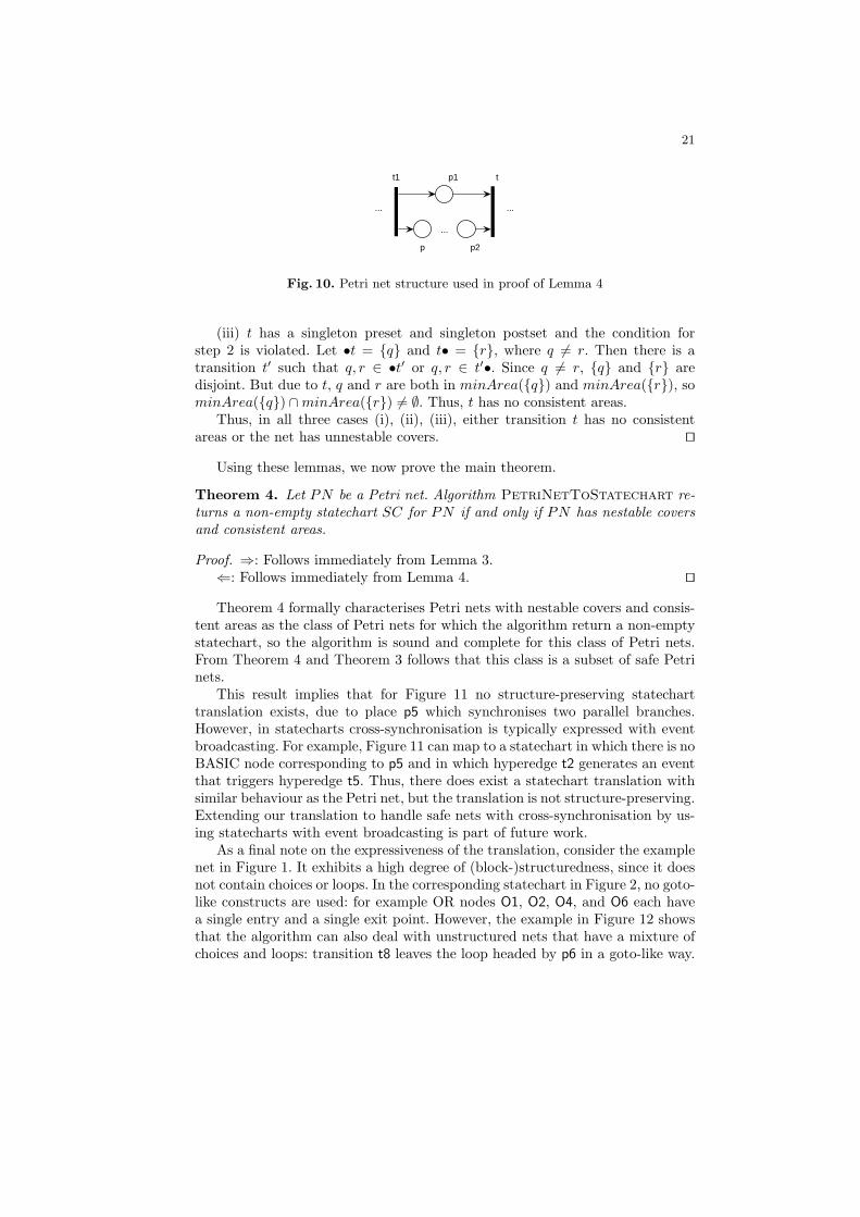
This result implies that for Figure 11 no structure-preserving statecharttranslation exists, due to place p5 which synchronises two parallel branches.However, in statecharts cross-synchronisation is typically expressed with eventbroadcasting. For example, Figure 11 can map to a statechart in which there is noBASIC node corresponding to p5 and in which hyperedge t2 generates an eventthat triggers hyperedge t5. Thus, there does exist a statechart translation withsimilar behaviour as the Petri net, but the translation is not structure-preserving.Extending our translation to handle safe nets with cross-synchronisation by us-ing statecharts with event broadcasting is part of future work.
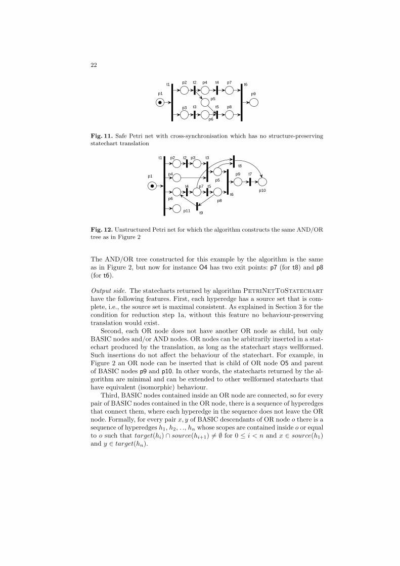
As a final note on the expressiveness of the translation, consider the examplenet in Figure 1. It exhibits a high degree of (block-)structuredness, since it doesnot contain choices or loops. In the corresponding statechart in Figure 2, no goto-like constructs are used: for example OR nodes O1, O2, O4, and O6 each havea single entry and a single exit point. However, the example in Figure 12 showsthat the algorithm can also deal with unstructured nets that have a mixture ofchoices and loops: transition t8 leaves the loop headed by p6 in a goto-like way.
22
t3
t1
p5p1
p2
p3
p4
p6
p7
p8
p9
t2 t4
t5
t6
Fig. 11. Safe Petri net with cross-synchronisation which has no structure-preservingstatechart translation
t1 t2 t3
p1
p2 p3
p4
p5
p6
p7
p8
p9
p10
p11
t4 t5
t6
t7
t9
t8
Fig. 12. Unstructured Petri net for which the algorithm constructs the same AND/ORtree as in Figure 2
The AND/OR tree constructed for this example by the algorithm is the sameas in Figure 2, but now for instance O4 has two exit points: p7 (for t8) and p8(for t6).
Output side. The statecharts returned by algorithm PetriNetToStatecharthave the following features. First, each hyperedge has a source set that is com-plete, i.e., the source set is maximal consistent. As explained in Section 3 for thecondition for reduction step 1a, without this feature no behaviour-preservingtranslation would exist.
Second, each OR node does not have another OR node as child, but onlyBASIC nodes and/or AND nodes. OR nodes can be arbitrarily inserted in a stat-echart produced by the translation, as long as the statechart stays wellformed.Such insertions do not affect the behaviour of the statechart. For example, inFigure 2 an OR node can be inserted that is child of OR node O5 and parentof BASIC nodes p9 and p10. In other words, the statecharts returned by the al-gorithm are minimal and can be extended to other wellformed statecharts thathave equivalent (isomorphic) behaviour.
Third, BASIC nodes contained inside an OR node are connected, so for everypair of BASIC nodes contained in the OR node, there is a sequence of hyperedgesthat connect them, where each hyperedge in the sequence does not leave the ORnode. Formally, for every pair x, y of BASIC descendants of OR node o there is asequence of hyperedges h1, h2, . ., hn whose scopes are contained inside o or equalto o such that target(hi) ∩ source(hi+1) 6= ∅ for 0 ≤ i < n and x ∈ source(h1)and y ∈ target(hn).
23
p2
p1
p3
p2
p3
p1 O1
O2
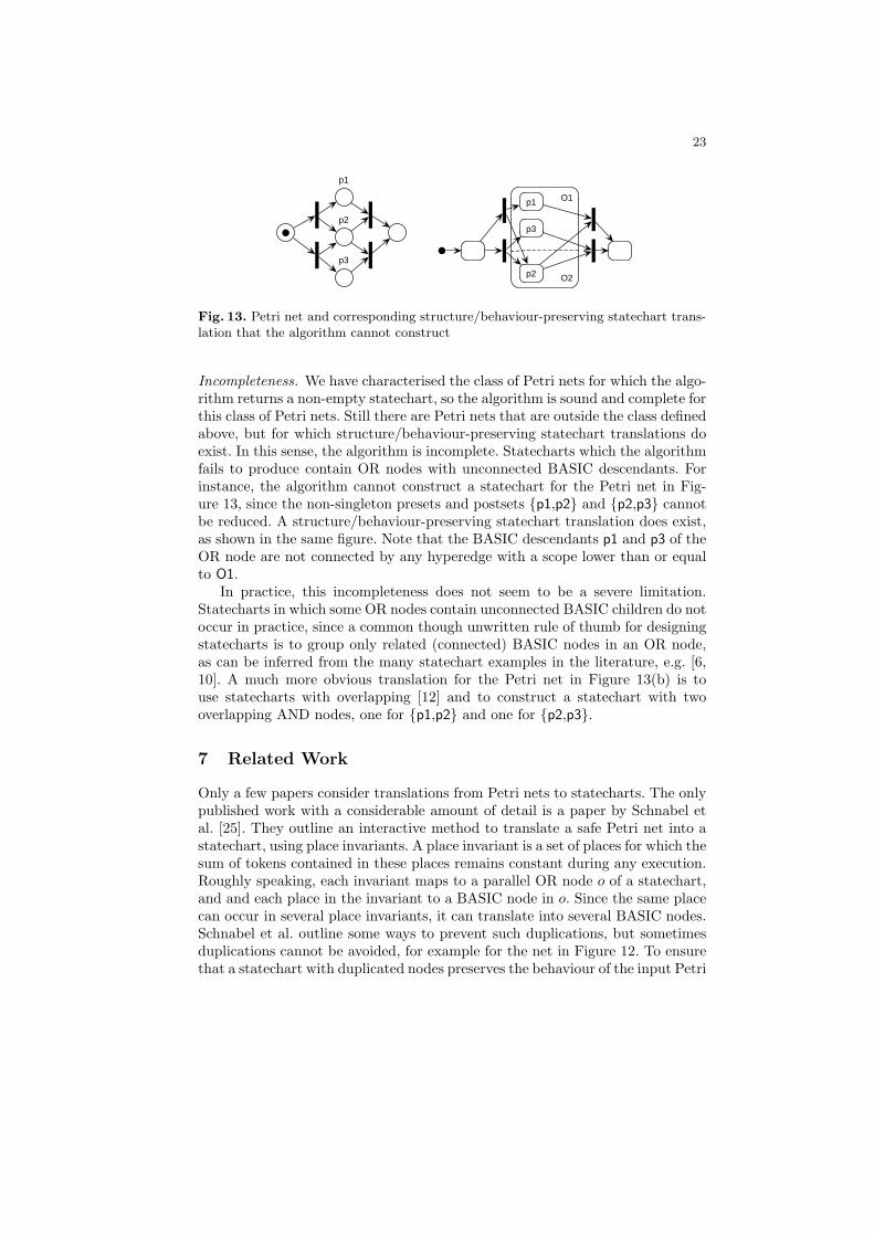
Fig. 13. Petri net and corresponding structure/behaviour-preserving statechart trans-lation that the algorithm cannot construct
Incompleteness. We have characterised the class of Petri nets for which the algo-rithm returns a non-empty statechart, so the algorithm is sound and complete forthis class of Petri nets. Still there are Petri nets that are outside the class definedabove, but for which structure/behaviour-preserving statechart translations doexist. In this sense, the algorithm is incomplete. Statecharts which the algorithmfails to produce contain OR nodes with unconnected BASIC descendants. Forinstance, the algorithm cannot construct a statechart for the Petri net in Fig-ure 13, since the non-singleton presets and postsets {p1,p2} and {p2,p3} cannotbe reduced. A structure/behaviour-preserving statechart translation does exist,as shown in the same figure. Note that the BASIC descendants p1 and p3 of theOR node are not connected by any hyperedge with a scope lower than or equalto O1.
In practice, this incompleteness does not seem to be a severe limitation.Statecharts in which some OR nodes contain unconnected BASIC children do notoccur in practice, since a common though unwritten rule of thumb for designingstatecharts is to group only related (connected) BASIC nodes in an OR node,as can be inferred from the many statechart examples in the literature, e.g. [6,10]. A much more obvious translation for the Petri net in Figure 13(b) is touse statecharts with overlapping [12] and to construct a statechart with twooverlapping AND nodes, one for {p1,p2} and one for {p2,p3}.
7 Related Work
Only a few papers consider translations from Petri nets to statecharts. The onlypublished work with a considerable amount of detail is a paper by Schnabel etal. [25]. They outline an interactive method to translate a safe Petri net into astatechart, using place invariants. A place invariant is a set of places for which thesum of tokens contained in these places remains constant during any execution.Roughly speaking, each invariant maps to a parallel OR node o of a statechart,and and each place in the invariant to a BASIC node in o. Since the same placecan occur in several place invariants, it can translate into several BASIC nodes.Schnabel et al. outline some ways to prevent such duplications, but sometimesduplications cannot be avoided, for example for the net in Figure 12. To ensurethat a statechart with duplicated nodes preserves the behaviour of the input Petri
24
A
t1 t2 t3 t4
t1 t2 t3 t4
p1p2
p3
p4
p5
p6
p7
p8
p9
p10
p1
p2
p3
p4
p5
p6
p7
p8
p10
p9
Fig. 14. Petri net with matching transition pairs and a structure/behaviour-preservingstatechart translation
net, Schnabel et al. make use of event synchronisation and auxiliary variables.However, their solution is specific to StateFlow statecharts [17]. There are threemain differences that distinguish our work from theirs. First, our approach doesnot duplicate places, so it does not require event-synchronisation or auxiliaryvariables. Next, the translation algorithm defined in this paper is fully automatedwhile their method requires user interaction. Finally, unlike Schnabel et al., wehave formally proven the correctness of the algorithm and characterised theexpressiveness of the translation, both from the input side (class of safe Petrinets that can be translated successfully) and the output side (class of statechartsconstructible by the translation).
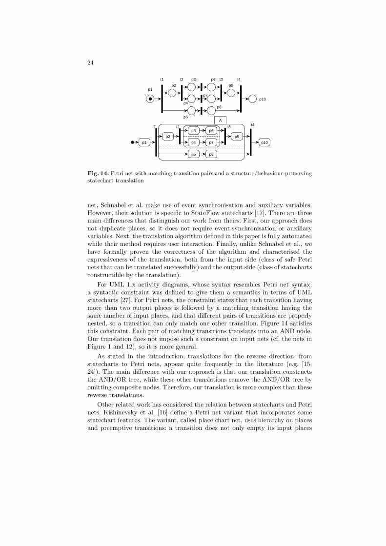
For UML 1.x activity diagrams, whose syntax resembles Petri net syntax,a syntactic constraint was defined to give them a semantics in terms of UMLstatecharts [27]. For Petri nets, the constraint states that each transition havingmore than two output places is followed by a matching transition having thesame number of input places, and that different pairs of transitions are properlynested, so a transition can only match one other transition. Figure 14 satisfiesthis constraint. Each pair of matching transitions translates into an AND node.Our translation does not impose such a constraint on input nets (cf. the nets inFigure 1 and 12), so it is more general.
As stated in the introduction, translations for the reverse direction, fromstatecharts to Petri nets, appear quite frequently in the literature (e.g. [15,24]). The main difference with our approach is that our translation constructsthe AND/OR tree, while these other translations remove the AND/OR tree byomitting composite nodes. Therefore, our translation is more complex than thesereverse translations.
Other related work has considered the relation between statecharts and Petrinets. Kishinevsky et al. [16] define a Petri net variant that incorporates somestatechart features. The variant, called place chart net, uses hierarchy on placesand preemptive transitions: a transition does not only empty its input places
25
put also all descendant places of the input places. However, the relation betweenplace chart nets and Petri nets is not formally analysed.
Drusinsky and Harel [4] show that a class of concurrency models that includesboth statecharts and Petri nets is more succinct than finite state machines.However, they do not explicitly make a distinction between statecharts and Petrinets, i.e., these fall in the same class.
Finally, in previous work [5] we defined an algorithm for translating Petrinets to statecharts. However, that algorithm is much more complex and lessefficient than the algorithm described in this paper.
8 Conclusion
A polynomial algorithm has been defined that translates safe Petri nets to stat-echarts in a structure-preserving way, so constructed statecharts resemble theinput nets. The algorithm is structural and does not use any Petri net analy-sis technique. Moreover, it preserves the behaviour of the input net. Since thealgorithm is polynomial, it is also efficient for large Petri nets. Next, we havecharacterised the class of nets for which the translation algorithm returns a non-empty statecharts. Thus, the algorithm is sound and complete for this class ofnets.
There are several directions for further work. First, by considering state-charts with event broadcasting, the translation can be extended to deal with abroader class of safe nets. Also, the algorithm can be extended to statechartswith overlapping [12]. On the more applied side, the algorithm can be used as afoundation for implementing model transformations between UML activity dia-grams, which resemble Petri nets, and UML statecharts [27]. Activity diagramscan specify the stateful behaviour of objects, whose lifecycles are independentlyspecified in UML statecharts. The translation algorithm can be used to trans-form object behaviour specified in UML activity diagrams into UML statecharts,either to check consistency with an existing object lifecycle or to synthesise anobject lifecycle from scratch.
References
1. M. Ajmone Marsan, G. Balbo, G. Conte, S. Donatelli, and G. Franceschinis. Mod-elling with Generalized Stochastic Petri Nets. J. Wiley, 1995.
2. E. Best, P. Darondeau, and H. Wimmel. Making Petri nets safe and free of internaltransitions. Fundamenta Informaticae, 80(1-3):75–90, 2007.
3. J. Desel and G. Juhas. What is a Petri net? Informal answers for the informedreader. In H. Ehrig, G. Juhas, J. Padberg, and G. Rozenberg, editors, UnifyingPetri Nets, Lecture Notes in Computer Science 2128, pages 1–27. Springer, 2001.
4. D. Drusinsky and D. Harel. On the power of bounded concurrency I: Finite au-tomata. Journal of the ACM, 41(3):517–539, 1994.
5. R. Eshuis. Statecharting Petri nets. Beta Working Paper Series, WP 153, Eind-hoven University of Technology, 2005.

26
6. R. Eshuis. Reconciling statechart semantics. Science of Computer Programming,74(3):65–99, 2009.
7. J. Esparza. Reduction and synthesis of live and bounded free choice Petri nets.Information and Computation, 114(1):50–87, 1994.
8. B. Grahlmann. The PEP tool. In O. Grumberg, editor, Proc. CAV ’97, LectureNotes in Computer Science 1254, pages 440–443. Springer, 1997.
9. O. Grumberg and S. Katz. Veritech: a framework for translating among modeldescription notations. STTT, 9(2):119–132, 2007.
10. D. Harel. Statecharts: A visual formalism for complex systems. Science of Com-puter Programming, 8(3):231–274, 1987.
11. D. Harel. On visual formalisms. Communications of the ACM, 31(5):514–530,1988.
12. D. Harel and C.-A. Kahana. On statecharts with overlapping. ACM Transactionson Software Engineering and Methodology, 1(4):399–421, 1992.
13. D. Harel and A. Naamad. The STATEMATE semantics of statecharts. ACMTransactions on Software Engineering and Methodology, 5(4):293–333, 1996.
14. D. Harel, A. Pnueli, J. P. Schmidt, and S. Sherman. On the formal semantics ofstatecharts. In Proceedings of the Second IEEE Symposium on Logic in Computa-tion, pages 54–64. IEEE, 1987.
15. G. Huszerl, I. Majzik, A. Pataricza, K. Kosmidis, and M. Dal Cin. Quantitativeanalysis of UML statechart models of dependable systems. Computer Journal,45(3):260–277, 2002.
16. M. Kishinevsky, J. Cortadella, A. Kondratyev, L. Lavagno, A. Taubin, andA. Yakovlev. Coupling asynchrony and interrupts: Place chart nets. In P. Azemaand G. Balbo, editors, Proc. ICATPN 1997, Lecture Notes in Computer Science1248, pages 328–47. Springer, 1997.
17. The Mathworks. Stateflow users guide, 2009. http://www.mathworks.com.18. T. Murata. Petri nets: Properties, analysis, and applications. Proc. of the IEEE,
77(4):541–580, 1989.19. C. A. Petri. Kommunikation mit Automaten. PhD thesis, Institut fur instru-
mentelle Mathematik, Bonn, 1962.20. A. Pnueli and M. Shalev. What is in a step: On the semantics of statecharts. In
T. Ito and A.R. Meyer, editors, Theoretical Aspects of Computer Software, LectureNotes in Computer Science 526, pages 244–265. Springer, 1991.
21. M. Rausch and B. Krogh. Transformations between different model forms in dis-crete event systems. In Proc. IEEE SMC 1997, volume 3, pages 2841–2846, 1997.
22. W. Reisig. Petri Nets: An Introduction. Number 4 in EATCS Monographs onTheoretical Computer Science. Springer, 1985.
23. W. Reisig and G. Rozenberg, editors. Lectures on Petri nets I: Advances in Petrinets, Lecture Notes in Computer Science 1492. Springer, 1998.
24. J.A. Saldhana, S.M. Shatz, and Z. Hu. Formalization of object behavior andinteractions from UML models. International Journal of Software Engineeringand Knowledge Engineering, 11(6):643–673, 2001.
25. M. Schnabel, G. Nenninger, and V. Krebs. Konvertierung sicherer Petri-netze instatecharts (in German). Automatisierungstechnik, 47(12):571–580, 1999.
26. IBM Rational Software. Rose, 2009. http://www.ibm.com/software/rational.27. UML Revision Taskforce. OMG UML Specification v. 1.5. Object Management
Group, 2003. OMG Document Number formal/2003-03-01.28. UML Revision Taskforce. UML 2.0 Superstructure Specification. Object Manage-
ment Group, 2003. OMG Document Number ptc/03-07-06.