Transitioning from Repeated Measures ANOVA to Mixed‐ModelsANOVA to Mixed‐Models

ERSH 8310

Today’s Class

• An introduction to modern versions of repeated measures ANOVAMixed models

• Mixed models are powerful tools for a lot of research applications:Repeated measuresLongitudinal data (i.e, growth models)Clustered data (i.e., hierarchical linear models)

• If you stare at them long enough you get even more statistical methods out of mixed models:out of mixed models:

Confirmatory Factor Analysis/Structural Equation ModelingItem Response Models

l d d l h h ll• Plus, mixed models operate using a estimation techniques that allow for missing data

Today’s Data Set – Same as Before

• Consider an experiment in which college students search for a particular letter in a string of letters on a computer screen

Half of the time the letter occurs in the string, and half of the time it does not

• On one third of the trials the letter string is a word g(condition a1), on one third it is a pronounceable nonword(a2), and on one third it is an unpronounceable set of random letters (a3)random letters (a3)

• The response measure is the average speed with which subjects correctly detect the target letter, measured in illi dmilliseconds

• The experiment is a single‐factor AxS design with a=3 types of letter stringsof letter strings

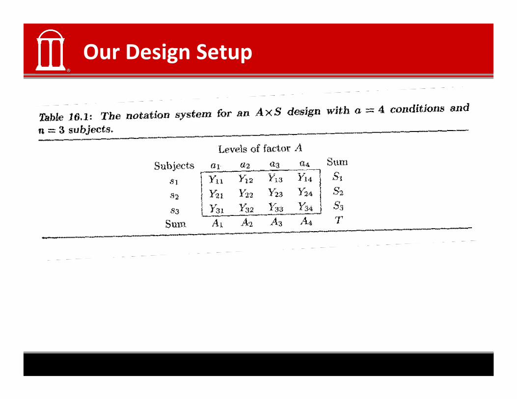
Our Design Setup

The Old Style of Analysis

• Prior to running the repeated measures analysis, let’s imagine we tried using what we already know about g g yANOVA:

Let’s run the analysis as if we have subjects nested within each factor (not crossed)

The Data Looks Like…

• This is what we call long data

• Every dependent variable value has a row• Every dependent variable value has a row

Old Analysis – No Repeated Measures

Our Statistical Model

• Recall our basic one‐way ANOVA statistical model:

• Likely the key assumption of the model was independenceijjTij EY ++= αμ

• Likely the key assumption of the model was independence of error terms

Caged as independence of observations

• Error was assumed have a variance of σ2error

• For our repeated measures analysis, however, we get three observations per person

People’s scores are highly correlatedp g y

Model Implied Covariance Matrix

• Within a subject, the ANOVA model assumes the following covariance matrixg

Shown for our three repeated observations exampleA covariance matrix is an un‐standardized correlation matrix

⎥⎥⎤

⎢⎢⎡

=→⎥⎥⎤

⎢⎢⎡

= 2

2

2

2

0000

0000

error

error

error

error

σσ

σσ

VR⎥⎥

⎦⎢⎢

⎣⎥⎥

⎦⎢⎢

⎣22 0000 error

error

error

error

σσ

The variances are all equal (homogeneity of variance)A zero covariance means a pair of observations are independent (the ANOVA independence assumption)independent (the ANOVA independence assumption)

Remember These Numbers

• From our ANOVA table treating the observations as not being repeated:g p

302.0;299.12

==A pF

• Which implies

233.606ˆ 2 =errorσ• Which implies

⎥⎤

⎢⎡

⎥⎤

⎢⎡

0233606000233.606

ˆ0233606000233.606

ˆ VR⎥⎥⎥

⎦⎢⎢⎢

⎣

=→⎥⎥⎥

⎦⎢⎢⎢

⎣

=233.60600

0233.6060233.60600

0233.6060 VR

Then There Was Repeated Measures ANOVA

• Next, we had repeated measures ANOVA…

( ) ESSY ++++= ααμ• However, because of our design (one observation within cell per person), the person by factor interaction

( ) ijijijTij ESSY ++++= ααμ

within cell per person), the person by factor interaction was the error term, leaving:

ESY +++• It assumed a weaker form of compound symmetry

ijijTij ESY +++= αμIt assumed a weaker form of compound symmetry (called sphericity) for the error terms

All errors had the same varianceAll covariances were the same

Repeated Measures: Data File in SPSS

The data are arranged in a wide-format:

One variable per- One variable per column.

Computational Formulas

• The computational formulas for the A ×S design are presented in Table 16.2 p

Note that dfT = an ‐ 1 that is one less than the total number of observations

Running the Analysis

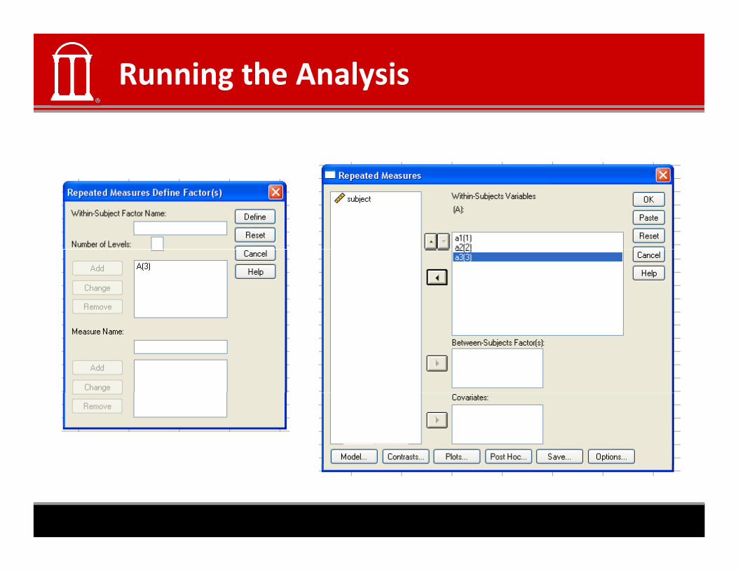
Running the Analysis

Analysis Output: SPSS

• There are two relevant parts to SPSS‐ a test for the factor

And:• And:

Analysis Output: Table 16.3

Matching Output to Interpretation

Source: ASource: A

Source: SxANow errorNow error

Source: S –Not typically interpretedp

Remember These Numbers

• From our ANOVA table treating the observations as not being repeated:g p

001.0;432.1422

==A pF

• But what about the original variance of error?

567.54ˆˆ 22 == AxSerror σσ• But…what about the original variance of error?

• It is now separated into two components (piles?)…Originally was 606.233Originally was 606.233Our new term is 54.567, leaving 551.67 behind…

The pile left behind now becomes the covariance

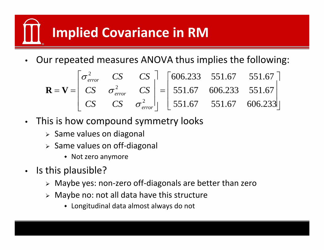
Implied Covariance in RM 

• Our repeated measures ANOVA thus implies the following:

⎤⎡⎤⎡ 67551675512336062 CSCSσ

⎥⎥⎥

⎦

⎤

⎢⎢⎢

⎣

⎡=

⎥⎥⎥

⎦

⎤

⎢⎢⎢

⎣

⎡

==233.60667.55167.55167.551233.60667.55167.55167.551233.606

2

2

error

error

error

CSCSCSCSCSCS

σσ

σVR

• This is how compound symmetry looksSame values on diagonal

⎦⎣⎦⎣

Same values on off‐diagonalNot zero anymore

• Is this plausible?Is this plausible?Maybe yes: non‐zero off‐diagonals are better than zeroMaybe no: not all data have this structure

L it di l d t l t l d tLongitudinal data almost always do not

And…Multivariate???

• The book had mentioned another approach, one called the multivariate approach.

• The multivariate approach looks for differences in the three factor levels simultaneously by looking at all data together

Uses a matrix‐algebra extension of statisticsUses a matrix algebra extension of statisticsTaught in ERSH 8350

h• Estimates every term in the covariance matrix RNeeds more dataLess powerful when compound symmetry holdsLess powerful when compound symmetry holds

Getting Full Covariance Estimates in SPSS

Under Options (in RM ANOVA), check the “Residual SSCP matrix” box

The “Unstructured” (FULL) R Matrix

Note: When using the univariate tests (F) theunivariate tests (F), the unstructured R matrix is not used for calculations.

It is only used in the Multivariate approach.

⎥⎤

⎢⎡

⎥⎤

⎢⎡ 4.4534.6378.5401312

21error σσσ

⎥⎥⎥

⎦⎢⎢⎢

⎣

=⎥⎥⎥

⎦⎢⎢⎢

⎣

==3.4242.5644.4532.5646.8534.637

22313

232

12

3

2

error

error

σσσσσσVR

So..Which R Matrix is Right?

Compound UnstructuredIndependence

⎥⎤

⎢⎡ 2 00errorσ

⎥⎤

⎢⎡ 7.5517.5512.606

⎥⎤

⎢⎡ 4.4534.6378.540

Symmetryp

⎥⎥⎥

⎦⎢⎢⎢

⎣2

2

0000

error

error

σσ

⎥⎥⎥

⎦⎢⎢⎢

⎣ 2.6067.5517.5517.5512.6067.551

R t d M

⎥⎥⎥

⎦⎢⎢⎢

⎣ 3.4242.5644.4532.5646.8534.637

M l i iRegular ANOVA Repeated Measures ANOVA

Multivariate ANOVA

Restrictive Assumptions

Few

Relaxed Assumptions

MoreFew Parameters

More Parameters

Enter…the Mixed Model

• Mixed‐effects models get their name from the combination of fixed effects (our treatment effects α) and random effects (our subject effects S)(our subject effects S)

• In their most basic form, they mimic the varying types of ANOVA models

Can fit differing structures for R/V matrices

• Using a different method of estimation (likelihood based), they:

Give less biased estimates of variances/covariancesGive less biased estimates of variances/covariancesA measure of which structure is correct (independence, CS, unstructured, etc…)The ability to incorporate missing data directly

d h l f lNo need to throw away incomplete cases or impute for missing values

The Mixed Model 

• The mixed model looks very similar to ANOVA:

The difference is our assumptions:

ijijTij ESY +++= αμ• The difference is our assumptions:

μT is a “fixed” effect – no estimate of variabilityαj are “fixed” effects – no estimate of variabilityj ySi are “random” effects – have normal distribution with zero mean and variance τ2

Called “random intercepts” each subject has a center pointCalled  random intercepts  – each subject has a center point

Eij are “random” – as usualHave normal distribution with zero mean and variance σ2error

The OLD ANOVA Model, Redefined

ijjTij EY ++= αμ jjj

• Model for the Means (Predicted Values):• Each person’s expected (predicted) outcome is a function of his/her• Each person s expected (predicted) outcome is a function of his/her 

treatment group (or values on covariates, and their interactions)• IV and DV are each measured only once per person (i subscript)

• Model for the Variance:

• Eij ~ N (0, σe2) ONE residual (unexplained) deviation• Eij has a mean of 0 with some estimated constant variance (σe2), 

is normally distributed, is unrelated to the IV, and is unrelated across people (across all observations, just people here)

Adding Within‐Person Variance to the Model for the Variances

Full Sample Distribution: 3 People, 5 Occasions eachFull Sample Distribution:

120

140

3 People, 5 Occasions each

100

120

60

80

20

40

Mean = 89.55Std. Dev. = 15.114N = 1,334

20

Empty +Within‐Person Model

Start off with Mean of Y as140 Start off with Mean of Y as “best guess” for any value:

= Grand Mean120

100

= Fixed Intercept

Can make better guess by

100

80

Can make better guess by taking advantage of repeated observations:

60

40

= Person Mean

Random Intercept

20

p

Empty +Within‐Person Model

Variance of Y  2 sources:

Between‐Person Variance:Differences from GRAND mean

140

120

INTER‐Individual Differences

Within Person Variance:

100

80Within‐Person Variance:

Differences from OWN meanINTRA‐Individual DifferencesThi i l b bl h h

60

40This part is only observable through longitudinal data20

General Linear Model for +Within‐Person Analysis

ijijTij ESY +++= αμ

y

ijijTij μ• Model for the Means (Predicted Values):

• Same model for means, except that DV and IV are measured more than once per person (predicted Y per treatment/time per person)than once per person (predicted Y per treatment/time per person)

• Model for the Variance (2 piles now):• E ~ N (0 σ 2) e has a mean of 0 and some estimated constant• Eij  N (0, σe ) eti has a mean of 0 and some estimated constant 

variance (σe2), is normally distributed, is unrelated to the IV, and is unrelated across people and time

• Si ~ N (0, τ2) mean differences across peopleSi  N (0, τ )  mean differences across people• Si has a mean of 0 and some estimated constant variance (τ2), is 

normally distributed, is unrelated to the IV, and is unrelated across people (constant over time within a person)

Mixed Models in SPSS

• Long Data Needed:                             Mixed Models:

Start By Putting Subject Variable in…

Then Add DV and Factors…And Choose Fixed/Random/

Three Analyses

• We will run all 3 types of ANOVA models from here:IndependencepCompound Symmetry (Now Random Intercept…was Repeated Measures)U t t d ( M lti i t )Unstructured (was Multivariate)

W ill th lt b t ill t f• We will see the same results, but will get a sense of what covariance structure to use

Can use most powerful test for fixed effectsCan use most powerful test for fixed effects

Independence ANOVA, Old and New

• Numbers from old:

233606ˆ302.0;299.1

2

==A pF

233.6062 =errorσ

⎥⎥⎥⎤

⎢⎢⎢⎡

= 0233.606000233.606

V̂⎥⎦⎢⎣ 233.60600

Compound Symmetry/Random Intercept

001.0;432.14 ==A pF

567.54ˆˆ;

22 == AxSerror

A p

σσ

⎤⎡ 755175512606

⎥⎥⎥⎤

⎢⎢⎢⎡

= 7.5512.6067.5517.5517.5512.606

V̂⎥⎦⎢⎣ 2.6067.5517.551

Unstructured

• Multivariate tests…not run

⎥⎤

⎢⎡

2564685346374.4534.6378.540

V̂⎥⎥⎥

⎦⎢⎢⎢

⎣

=3.4242.5644.4532.5646.8534.637V

What One is Best? Use Information Criteria

• We can use the model with the smallest information criterion

For simplicity we will use BIC

d d• Independence: 146.760• Compound Symmetry: 130.574U t t d 136 645• Unstructured: 136.645

The winner is:• The winner is: Compound symmetry – our RM ANOVA modelWe can now interpret the findings

Wrapping Up…

• Mixed models are powerful tools that are frequently used in research designsg

Repeated measuresLongitudinal dataHierarchical data

Today’s class was a first pass at how the models work• Today s class was a first pass at how the models work and what comes from them

To learn more, take a course in HLM or growth modelsTo learn more, take a course in HLM or growth models

• Thank you for a great semestery g

Up Next…

• Final discussion

I L b• In Lab:How to do mixed models in SPSS

• Homework:Study for the final (12/16 at 3:30 pm)

• Next week:No class (reading day)

Have a good break

• The week after:Final exam here at 3:30pm on 12/16