transition path sampling throwing ropes …jtaylor/teaching/fall2010/apm530/papers/... ·...

5 Apr 2002 12:52 AR AR155-11.tex AR155-11.SGM LaTeX2e(2001/05/10)P1: GSR10.1146/annurev.physchem.53.082301.113146

Annu. Rev. Phys. Chem. 2002. 53:291–318DOI: 10.1146/annurev.physchem.53.082301.113146

Copyright c© 2002 by Annual Reviews. All rights reserved

TRANSITION PATH SAMPLING: Throwing RopesOver Rough Mountain Passes, in the Dark

Peter G. BolhuisDepartment of Chemical Engineering, Nieuwe Achtergracht 166, 1018 WV Amsterdam,The Netherlands; e-mail: [email protected]

David ChandlerDepartment of Chemistry, University of California, Berkeley, California 94720;e-mail: [email protected]

Christoph DellagoDepartment of Chemistry, University of Rochester, Rochester, New York 14627;e-mail: [email protected]

Phillip L. GeisslerDepartment of Chemistry and Chemical Biology, Harvard University, Cambridge,Massachusetts 02138; e-mail: [email protected]

Key Words potential surfaces, kinetics, transition states, complex systems,trajectories, basins of attraction, rare events

■ Abstract This article reviews the concepts and methods of transition path sam-pling. These methods allow computational studies of rare events without requiring priorknowledge of mechanisms, reaction coordinates, and transition states. Based upon astatistical mechanics of trajectory space, they provide a perspective with which timedependent phenomena, even for systems driven far from equilibrium, can be examinedwith the same types of importance sampling tools that in the past have been applied sosuccessfully to static equilibrium properties.

INTRODUCTION

During the past several years, we and our coworkers have developed a general com-putational method for finding the transition pathways for infrequent events in bothequilibrium and nonequilibrium systems (1–14). The method requires no precon-ceived notion of mechanism or transition state. Called “transition path sampling,”it is metaphorically akin to throwing ropes over rough mountain passes, in the dark.“Throwing ropes” in the sense that one shoots short trajectories, attempting to reachone stable state from another. “In the dark” because high-dimensional systems areso complex that it is generally impossible to literally visualize the topography

0066-426X/02/0601-0291$14.00 291

5 Apr 2002 12:52 AR AR155-11.tex AR155-11.SGM LaTeX2e(2001/05/10)P1: GSR

292 BOLHUIS ET AL.

of relevant energy surfaces. In such cases, it is unlikely that the first throw ofthe rope will be successful, but one can learn from failures; and there should bean optimum procedure, i.e., sequence of throws, with which success is obtainedefficiently. We have discovered and demonstrated this type of sequence, openingthe way for many heretofore impossible computational studies of the dynamicpathways of chemical and physical transformations in clusters and in condensedmaterials.

RARE BUT IMPORTANT EVENTS IN COMPLEX SYSTEMS

DISPARITY OF TIMESCALES Often, dynamical processes of interest occur on time-scales that are very long compared to the shortest significant timescale. For exam-ple, the dissociation of a weak acid in water might occur with a half-life of, say,1 ms, while elementary steps of molecular motions in water occur in 1 fs. Similarly,timescales for folding the smallest of proteins are in the range of microseconds tomilliseconds, whereas that for small-amplitude motions of amino acid side chainsand water solvent is again 1 fs.

This wide disparity of timescales can present serious computational challenges.For instance, consider a computed trajectory for a system containing a weak acidmolecule and a bath of a few hundred water molecules. Within one or two ordersof magnitude—depending on computing equipment and algorithm—1 s of com-putation time is required to advance the system for what would correspond to 1 fsof physical time. As such, typically 1012 s of computing time seems to be requiredto find one example of an event leading to acid dissociation. A representativesampling of pathways to dissociation would therefore seem to be an impracticalcomputational task.

TRANSITION STATE THEORY One way to get around this problem is to focus onthe dynamical bottleneck for the rare event—the transition state surface. In a rareevent, it is this surface or threshold that is rarely visited and thus rarely crossed. If itslocation is known, however, one may construct a scheme where the system is firstmoved reversibly to the transition state surface and then many fleeting trajectoriesare initiated from that surface. The first step determines the reversible work andthus the probability for reaching the transition state, and the subsequent trajectoriesdetermine the probability for successfully crossing the threshold. Together, theygive the rate for the rare event. This approach was pioneered by Anderson (15),Bennett (16), and Chandler (17). It has been recently reviewed by Anderson (18),and a tutorial on it has been written by Chandler (19). Elementary discussions arefound in textbooks [e.g., References (20, 21)]. Although theoretically sound, thistwo-step procedure is limited in applicability because it presupposes knowledgeof the transition state. In most interesting cases, transition state surfaces are notknown and not easily characterized.

DIFFICULTY OF IDENTIFYING TRANSITION STATE SURFACES For low-dimensionalsystems involving only a few atoms, transition state surfaces usually intersect


TRANSITION PATH SAMPLING 293

saddle points in the potential energy surface. In those cases, transition state sur-faces can be identified with various algorithms that examine gradients of the po-tential energy surface and systematically search for saddle points on that surface(22, 23). For higher-dimensional systems, however, the potential energy surfacewill typically contain many saddle points, most if not all of which are irrelevantto the dynamics that carries the system from one stable (or metastable) state toanother. Figure 1 illustrates this point. Explicit enumeration of saddle points is fea-sible for a cluster of the order of ten or fewer atoms, but this enumeration providesno means to distinguish saddle points that are dynamically irrelevant from thosethat are dynamically relevant. For complex chaotic systems—large polyatomicmolecules, large clusters, condensed phases, and so forth—potential energy sur-faces are rough on the scale of thermal energies,kBT , and dense in saddle points.Effectively, therefore, there is generally an uncountable number of saddle points.Searching for a few such points is therefore insufficient and likely irrelevant. In-stead, one wants to locate and sample the ensemble of true dynamical bottlenecks.This task can be accomplished with transition path sampling.

TRANSITION PATH SAMPLING

IMPORTANCE SAMPLING The basic idea is a generalization of standard MonteCarlo procedures (20, 21, 24, 25) that focuses upon chains of states constituting dy-namical trajectories (26) rather than upon individual states. In its standard form, aMonte Carlo calculation performs a random walk in configuration space. The walkis biased to ensure that the most important regions of configuration space are ade-quately sampled. Specifically, in a Monte Carlo random walk, configurationx is vis-ited in proportion to its probabilityp(x). The walk may be initiated far from a typi-cal configuration [i.e.,x far from values ofx where the weight fromp(x) is largest],but after some equilibration period, the bias drives the system to those importantregions of configuration space. This feature is crucial to the success of Monte Carlosampling. It is called importance sampling and is illustrated in Figure 2.

Importance sampling can be generalized to trajectory space, as we have doneto create the methods of transition path sampling. Consider the ensemble of alltrajectories that are, say, 1 ps long. Most of these trajectories will be localized nearsome basin of attraction—a long-lived collection of neighboring microstates. Raretransition state crossings will comprise a small subset of these 1-ps trajectories.For example, if the process of interest occurs roughly once every millisecond, thenonly one out of a billion 1-ps trajectories will exemplify that process. Transitionpath sampling provides an efficient means to sample such rare subensembles.

IMPORTANCE SAMPLING OF TRAJECTORY SPACE Let us suppose the rare processesof interest are transitions between states or regionsA andB. These regions arecharacterized by their respective population operators,hA(χ ) andhB(χ ). Here,χdenotes a point in phase space—configuration space and momentum space com-bined. (The applications of transition path sampling discussed in the following


294 BOLHUIS ET AL.

Figure 2 In a Metropolis Monte Carlo simulation, one generates a random walk inconfiguration space according to the probability distributionp(x) ∝ exp[−V(x)/kBT ].If the distribution were that of a canonical ensemble,V(x) would denote the potentialenergy for configurationx. Along this walk, a new configurationx′ is generated bydisplacing the old configurationx by a randomly chosen small step,1. Thenx′ isaccepted or rejected. If the step goes downhill in energy, i.e., if the new configurationhas a higher probability than the old one,x′ is always accepted. Uphill moves, onthe other hand, are only accepted with a probabilityw(x,1) p(x′)/p(x)w(x′,−1),wherew(x,1) is the distribution for the random step,1, given the configurationx. Inthis way, barriers of the order ofkBT or smaller do not hinder the random walk, anda system will move quickly to configurations of high probability (the lightly shadedregion) even when initiated far away from that important region in configuration space.

sections of this review use characteristic functions of configuration space,x, only,but this limitation is not required.) Whenχ is within regionA, hA(χ )= 1, other-wise,hA(χ ) = 0. The corresponding population operator for regionB, hB(χ ), issimilarly defined. Transitions between regionsA andB coincide with trajectoriesconnecting these regions. A trajectory of time durationt, χ (t) = (χ0, χ1, . . . , χt ),is a chronological sequence of phase space points generated by repeated applica-tion of a dynamical propagation rule. Trajectories we imagine are consistent withLiouville’s equation or one of its analogues (27, 28). Namely, they must be re-versible, must preserve the norm of the distribution of states, and must preserve anequilibrium distribution. For simplicity, but not for necessity, we might be consid-ering deterministic dynamics, in which caseχt is entirely determined by the initial



phase space point,χ0. The statistical weight for the rare trajectories connectingA andB is hA(χ0)ρ[χ (t)]hB(χt ), whereρ[χ (t)] is the unconstrained distributionfunctional for trajectories. For deterministic trajectories,

ρ[χ (t)] = ρ(χ0)∏

0<t ′≤t

δ[χt ′ − χt ′ (χ0)], 1.

whereρ(χ0) is the unconstrained distribution of initial phase space points,χ0. Tran-sition path sampling is done by carrying out a random walk in trajectory space,biased to be the importance sampling for the distributionhA(χ0)ρ[χ (t)]hB(χt ).Figure 3 illustrates how it is done in a practical and simple fashion.

In this perspective, stable or long-lived statesAandBmust be well characterizedat the outset. This characterization can be difficult, as we discuss below. Never-theless, we see that nothing need be presupposed about the dynamical pathways

Figure 3 Illustration of “shooting moves,” generating a random walk in trajectoryspace for Newtonian trajectories connecting regionsA andB. For example, trajectory2 is generated by changing trajectory 1 by a small amount. This change can be accom-plished, for example, by first choosing a time slice pointτ lying between 0 andt. At thistime slice, the momentum of trajectory 1 can be altered by some small randomly chosenamount. The resulting new momentum can be used along with the configuration of tra-jectory 1 at timeτ as the initial conditions for a new trajectory created by propagatingforward from that phase space point fort−τ steps and backward from that phase spacepoint forτ steps. Because regionsA andB remain connected, this second path will beaccepted as the new trajectory, provided the value ofρ(χ0) for the new trajectory com-pares favorably with that for the first trajectory. Specifically, the probability to attempta step from a trajectoryχ (t) = (χ0, χ1, . . . , χt ) toχ ′(t) = (χ ′0, χ

′1, . . . , χ

′t ) is the joint

probability for choosing time sliceτ and assigning a momentum changeδ at that timeslice,w(χ, τ, δ). The acceptance probability for that trial step is min[1, w(χ, τ, δ)hA(χ ′0) ρ(χ ′0) hB(χ ′t )/hA(χ0)ρ(χ0)hB(χt )w(χ ′, τ,−δ)]. By the same type of procedure,trajectory 3 is generated from trajectory 2. This time, however, the new path does notconnectAandB, and it is rejected. This sequence of acceptances and rejections ensuresthat the correct path ensemble is sampled—namely, the ensemble that is weighted by thedistributionhA(χ0)ρ(χ0)hB(χt ). There is great flexibility in the choice of random walksteps. This flexibility can be exploited in efforts to improve the efficiency of transitionpath sampling. In practice, shooting moves are only one of several moves employed intransition path sampling. References (2, 10, 62) describe other useful moves.


296 BOLHUIS ET AL.

(i.e., trajectories) that join these states. This feature is the major strength of themethod. Transition path sampling is a random walk through the ensemble of allpaths connectingA andB. From studying the trajectories visited during this walk,the nature of the dynamical pathways is discovered.

COMPUTATIONAL COST The computational effort in carrying out a transition pathsampling calculation scales linearly with the number of trajectories harvested. Thisscaling is optimum. In particular, to harvestN statistically independent transitionpathways of lengtht requires the same order of effort as that required to performa single trajectory of lengthN. In practice, random moves like those illustratedin Figure 3 are accepted with probabilities between 0.1 and 0.5. In addition, thecorrelations in that random walk persist typically for only two or three acceptedmoves. Thus, for instance, 1000 statistically independent 1 ps trajectories are ob-tained with roughly the same computational resources required for a single straight-forward trajectory of length 1–10 ns. The straightforward trajectory, however, willalmost certainly not show an example of a rare event occurring on the timescale of,say, 1 ms, while each of 1000 transition path trajectories will exhibit an independentexample of the event.

INITIAL TRAJECTORY Before the sampling of typical transition paths begins, onerequires a representative member of the ensemble of trajectories with distribu-tion hA(χ0)ρ[χ (t)]hB(χt ). This member, i.e., this first example of a typical trajec-tory linking regionsA andB, can be obtained in a variety of ways. All of theseways coincide with some sort of equilibration run. The situation is much likethat encountered in standard Monte Carlo. In that case, the Monte Carlo walkis initiated at some chosen configuration. The configuration may be far from atypical equilibrium configuration, as illustrated in Figure 2. Nevertheless, after re-peated steps in the random walk, each one satisfying detailed balance, the systemeventually reaches the region of typical equilibrium configurations. It is at thispoint where equilibrium sampling is initiated. Similarly, in transition path sam-pling, one may begin with literally no concept of a reasonable dynamical trajectory.Any initial path can be drawn to initiate an equilibration run. After equilibration,i.e., after the walk through trajectory space begins to visit trajectories typical ofthe weight functionalhA(χ0) ρ[χ (t)] hB(χt ), sampling can begin.

For example, suppose trajectories connecting regionsA andB are easily foundin a dynamical simulation run at a temperatureT ′, but the actual temperature ofinterest,T, is much smaller thanT ′. In other words, suppose one has examples oftrajectories taken from the distributionhA(χ0) ρ[χ (t); T ′] hB(χt ), but one wants tosample the distributionhA(χ0) ρ[χ (t); T ] hB(χt ). One may use the high-temperaturetrajectory taken from the former and initiate an equilibration run with the latter.If there is poor overlap between the distributionsρ[χ (t); T ′] and ρ[χ (t); T ], thisrun may be done in stages, lowering the temperature by only a fraction ofT ′ − Tat each stage.



Some initial paths may be farther from the desired ensemble than others, andsome equilibration walks may be slower than others. Nevertheless, this illustrationsshows that there is great flexibility as to how one may proceed. We discuss thispoint further below.

REVERSIBLE WORK

Standard Monte Carlo sampling of microstates follows from the principles of equi-librium statistical mechanics, and quantities computed from it are thermodynamicproperties. Similarly, transition path sampling follows from a statistical mechan-ics of trajectory space, and quantities computed from it are dynamical properties,like rate constants. The two techniques share an important similarity—namely,they both move through their respective spaces (configuration space and trajectoryspace) in fashions that preserve their prescribed distributions. In other words, theyboth obey conditions of detailed balance. This similarity can be used to establishan isomorphism between thermodynamical quantities and dynamical properties.The isomorphism is of practical importance because it makes accessible to thestudy of dynamics all the computational advantages of methods used to determinethe statistics of rare configurations in an equilibrium system.

REVERSIBLE WORK IN EQUILIBRIUM STATISTICAL MECHANICS To illustrate the iso-morphism, consider first the traditional connection between thermodynamics andequilibrium statistical mechanics. The partition function associated with a ther-modynamic stateA, ZA, is the sum over the configurations that characterize stateA weighted by the distributionp(x), i.e., ZA =

∑xhA(x) p(x). (In the context

of equilibrium statistical mechanics, we define states in terms of configurationalvariables,x, rather than phase space variables,χ .) The reversible work to movefrom thermodynamic stateA to thermodynamic stateB, WAB, is the free energydifference between those states. Namely,

exp(−WAB/kBT) =∑

x hB(x) p(x)∑x hA(x) p(x)

, 2.

or WAB = −kBT ln(ZA/ZB). In addition, for a system with distributionp(x),exp(−WAB/kBT) is the probability that the system is found in stateB relativeto that of being found in stateA. As such, one may efficiently compute the relativeprobability for being in stateB, even when this probability is extremely small, i.e.,even whenWABÀ kBT . In particular, because reversible work is independent ofpath, it can be evaluated by moving the system reversibly through an arbitrarilychosen series of intermediate states. A specific reversible path is created by a spe-cific series of steps for convertinghA(x) to hB(x). For instance, one can introducea class of functions,h(λ)(x), that smoothly interpolate betweenhA(x) at λ = 0 tohB(x) atλ = 1. For a givenλ, the partition function isZ(λ) =∑x h(λ)(x) p(x), and


298 BOLHUIS ET AL.

provided thath(λ)(x) has a reasonable overlap withh(λ−1λ)(x), we can also write

Z(λ) =∑

x

[h(λ)(x)

/h(λ−1λ)(x)

]h(λ−1λ)(x)p(x)

= Z(λ−1λ)⟨h(λ)(x)

/h(λ−1λ)(x)

⟩λ−1λ, 3.

where 〈. . .〉λ denotes the average with distributionh(λ)(x)p(x). By applying thisresult over and over again, withλ = 1λ, 21λ, . . . ,1, the quantityZB/ZA isdetermined. In order to ensure reasonable overlap of adjacent distributions, thenumber of steps required in this procedure is of the order ofWAB/kBT, i.e.,1λ 'kBT/WAB. In contrast, a straightforward Monte Carlo sampling ofp(x) will providea reasonable estimate of the probability ratio,ZA/ZB, in a computational timescaleof t exp(WAB/kBT), where t is a typical sampling time, such as that to arriveat reasonable statistics for just stateA. This juxtaposition of linear vs. exponen-tial computational cost shows that wheneverWABÀ kBT , the stepwise proceduremakes feasible estimates that would be impossible to perform in a straightforwardsimulation.

REVERSIBLE WORK FOR CHANGING ENSEMBLES OF TRAJECTORIES With these ideasin mind, we now consider the “partition function” for trajectories of lengtht con-necting regionsA andB. Namely,

ZAB(t) =∑χ (t)

ρ[χ (t)] hA(χ0) hB(χt ). 4.

The sum overχ (t) denotes the sum over all trajectories (χ0, χ1, . . . , χt ). For de-terministic trajectories, Equation 4 reduces to

ZAB(t) =∑χ0

ρ(χ0) hA(χ0) hB(χt ), 5.

whereχt is determined solely byχ0. This partition function counts the number oftrajectories connectingA andB, weighted by the distribution functional,ρ[χ (t)].In contrast to this quantity, consider the similarly weighted number of trajectoriesthat begin inA and end anywhere,∑

χ (t)

ρ[χ (t)] hA(χ0) =∑χ0

ρ(χ0)hA(χ0) = ZA, 6.

where the first equality follows from the normalization of the distribution func-tional, and the second is true whenρ(χ ) is an equilibrium distribution—micro-canonical, or canonical, or so forth. In that case,ZAB(t) is the time correlationfunction, 〈hA(0)hB(t)〉. Here,〈. . .〉 denotes the equilibrium ensemble average overinitial conditions, andhB(t) is the population of stateB at timet. Thus, the ratio ofpartition functions,

ZAB(t)/ZA = 〈hA(0)hB(t)〉〈hA〉 , 7.



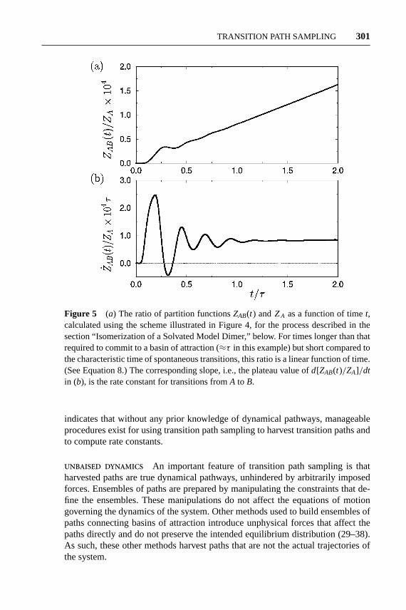
is the probability of finding the system in stateB a timet after it was in stateA. If AandBare separated by a single dynamical bottleneck, this probability will increasefrom 0 to 〈hB〉 with a time dependence that is exponential after a transient time,τmol. The transient time is the typical time for a trajectory to cross the bottleneckand commit to one of the two basins of attraction. It is a relatively short time, farshorter than the exponential relaxation time,τrxn = 1/(kAB+ kBA), wherekAB isthe rate constant for transitions fromA to B, andkBA is that for reverse transitions(17). As such, the rate constant for transitions fromA to B can be computed as aratio of partition functions,

ZAB(t)/ZA = kAB t, τmol < t ¿ τrxn. 8.

The first inequality,τmol < t , establishes the appropriate length for the trajecto-ries harvested by transition path sampling for the crossing of a single bottleneck.Trajectories should be long enough to show thatZAB(t)/ZA grows linearly in time.Trajectories of shorter length will be atypical of the transition path ensemble. Incases whereB is not reached fromA in typically one step, but through one or moreintermediate long-lived states,ZAB(t)/ZA will not exhibit linear behavior after ashort period of time. This fact provides a criterion that can be used to discover theexistence of intermediate states (2).

The partition functionZAB(t) converts toZA when the population operatorhB(χ )is converted to unity. Hence,− kBT ln[ZAB(t)/ZA] can be viewed as the reversiblework to change from the ensemble of trajectories initiated inA to the ensembleof trajectories connecting regionsA andB. Furthermore, this work is independentof the specific path, provided the steps are taken reversibly. In other words, witha slight change in notation, the second equality in Equation 3 can apply to thecalculation ofZAB(t)/ZA—namely,

Z(λ)(t) = Z(λ−1λ)(t)⟨h(λ)(χt )

/h(λ−1λ)(χt )

⟩λ−1λ 9.

whereh(λ)(χ ) interpolates between 1 atλ = 0 andhB(χ ) at λ = 1, and 〈. . .〉λdenotes the average over trajectories of lengtht weighted by the distribution pro-portional tohA(χ0) ρ(χ0) h(λ)(χt ). As such,Z(λ)(t) changes fromZA whenλ = 0to ZAB(t) whenλ = 1. As in the standard equilibrium case, Equation 3, the dynam-ical formula (9) is to be applied with a choice ofh(λ)(χ ) that allows for reasonableoverlap between adjacent ensembles. In addition, as in the equilibrium case, the dy-namical formula (9) provides the basis for computing the desired partition functionratio with linear rather than exponential computational effort.

STEPWISE ROUTE TO THE INITIAL TRAJECTORY Finally, by converting from theensemble where trajectories begin inA to the ensemble where trajectories linkAandB, the stepwise procedure provides a method for preparing the initial trajectory fortransition path sampling. It is a laborious preparation, moving from one ensemble tothe next. For specific situations, more efficient preparation schemes can be devised,as we discuss below. Nevertheless, this example, illustrated in Figures 4 and 5,


300 BOLHUIS ET AL.

Figure 4 Schematic sequence of trajectory ensembles, with distribution function-als hA(χ0)ρ[χ (t)] h(λ)(χt ), changing fromλ = 0 to λ = 1. Dashed lines surroundregions whereh(λ)(χ ) is nonzero. Forλ = 0, trajectories may end anywhere inthe accessible phase space. Forλ = 1, trajectories must end in stateB. In the ini-tial stages of the sequence, the transition state surface lies within the region de-fined by h(λ)(χ ), and typical trajectories remain in the basin of attraction of stateA. In the latter stages, the transition state surface lies outside the region defined byh(λ)(χ ), so that trajectories must cross the separatrix and typically continue deepinto the basin of attraction of stateB. This scheme will generally succeed at creatingthe desired final ensemble of trajectories passing fromA to B, but the scheme is notsatisfactory for computing rate constants. A satisfactory scheme must reach the finalensemble reversibly. The latter stages of the sequence illustrated in this figure willusually fail to be reversible, because they do not efficiently sample trajectories thatend near the transition state surface on the side of stateB. To ensure reversibility,this scheme can be modified to use a sequence of more confined “window” ensem-bles (4), much as is done with umbrella sampling in equilibrium statistical mechanics(20, 21, 24, 25). Thei th such window includes only trajectories that end in the regiondefined byh(λi−1)(χ )[1 − h(λi+1+1)(χ )]. Here,1 is a small, positive number that al-lows for reasonable overlap between adjacent ensembles. With appropriately chosenvalues forλi , the reversible work is comparable tokBT for each step in this modifiedscheme.



Figure 5 (a) The ratio of partition functionsZAB(t) andZA as a function of timet,calculated using the scheme illustrated in Figure 4, for the process described in thesection “Isomerization of a Solvated Model Dimer,” below. For times longer than thatrequired to commit to a basin of attraction (≈τ in this example) but short compared tothe characteristic time of spontaneous transitions, this ratio is a linear function of time.(See Equation 8.) The corresponding slope, i.e., the plateau value ofd[ZAB(t)/ZA]/dtin (b), is the rate constant for transitions fromA to B.

indicates that without any prior knowledge of dynamical pathways, manageableprocedures exist for using transition path sampling to harvest transition paths andto compute rate constants.

UNBAISED DYNAMICS An important feature of transition path sampling is thatharvested paths are true dynamical pathways, unhindered by arbitrarily imposedforces. Ensembles of paths are prepared by manipulating the constraints that de-fine the ensembles. These manipulations do not affect the equations of motiongoverning the dynamics of the system. Other methods used to build ensembles ofpaths connecting basins of attraction introduce unphysical forces that affect thepaths directly and do not preserve the intended equilibrium distribution (29–38).As such, these other methods harvest paths that are not the actual trajectories ofthe system.


302 BOLHUIS ET AL.

DISTINGUISHING BASINS OF ATTRACTION Often, a significant challenge in tran-sition path sampling work is the characterization of the stable states. It requiresa choice of discriminating order parameters—variables that uniquely distinguishstatesA andB. Establishing that a variable, sayq, has mostly one range of valuesin one state and a nearly distinct range of values in the other is not sufficient. Theremust be no overlap between the region spanned byhA(χ ) and the basin of attrac-tion of stateB, and vice versa. Otherwise, sampling with the weight functionalρ[χ (t)] hA(χ0)hB(χt ) will fail to harvest trajectories crossing from one basin tothe other. This point is illustrated in Figure 6, and is exemplified by the difficulty

Figure 6 (a) Contours of a free energy surface,F(q,q′), for which the coordinateq does not successfully discriminate between the basins of attraction of statesA andB. Although the distributions ofq within A andB do not overlap, some microstatesbelonging to the basin of attraction ofA have values ofq characteristic ofB. (b) q asa function of time for the two trajectories sketched in (a). The trajectory depicted as asolid line makes a transition fromA to B, passing through the transition state surface.The trajectory depicted as a dashed line remains within the basin of attraction of stateA, but, when projected ontoq, appears to visit stateB. Transition path sampling withq as an order parameter would yield primarily trajectories of the latter type, which donot pass through the transition state surface.



of sampling pathways for excess proton transport in liquid water. In this appli-cation, basins of attraction for hydronium ion structures are poorly characterizedby molecular geometries (39) and weights of empirical valence bond states (40).Day et al. have attempted to circumvent this problem by studying proton transfer,from a hydronium ion to a nearby water molecule, through an intervening watermolecule (41). Because the order parameter Day et al. use may not distinguishamong the pertinent states, however, it is possible that the trajectories they haveharvested do not represent true proton transfer events. These pathways may com-prise instead large fluctuations within the basin of attraction of the intermediatestate. In our experience, identifying discriminating order parameters can involvea significant degree of experimentation, performing transition path sampling withvarious choices of order parameters until a satisfactory discriminating choice isdetermined.

COMMITTORS, THE SEPARATRIX, ANDTHE TRANSITION STATE ENSEMBLE

Harvested transition paths can be examined to determine examples of configura-tions lying on the transition state surface. This examination is done with the con-cepts of committors and the separatrix. The committor,pA(x, ts), is the probability(or fraction) of fleeting trajectoriesχ (ts) initiated from configurationx to end instateA a short timets later—namely,

pA(x, ts) =∑χ (ts)

ρ[χ (ts)] δ(x0− x) hA(χ ts)/p(x), 10.

where theδ-function has unit weight when the initial configuration of the fleetingtrajectory,x0, coincides withx and is zero otherwise. We often use the abbreviatedsymbolpA for the committor, leaving the dependence uponxandts to be understoodimplicitly. In the context of protein folding, this object has been calledpF—for“p-fold”—or (1 − pF), depending on whether the protein ends in a folded orunfolded state (42, 43). For the sequence of configurations visited in a specifictrajectory connectingA and B, (x0, x1, . . . , xτ , . . . , xt ), pA can be viewed as afunction ofτ. For physical situations where transitions betweenA andB exhibitthe typical timescale separationτmol ¿ τrxn, pA(τ ) will be either 1 or 0, exceptfor one or a few short periods of time where the function changes between thesetwo values. As illustrated in Figure 7, the short period(s) coincide with crossing(s)of the dynamical bottleneck. Thus, meaningful examination of the bottleneck isobtained from a committor if the short time,ts, is of the order of the commitmenttime,τmol. A time slice on a trajectory connectingA andB is committed to stateAif pB ¿ pA ' 1 for the configuration at that time slice. Here,pB is defined in thesame way aspA. Similarly, a time slice is committed to stateB if pA ¿ pB ' 1.On the other hand, a time slice wherepA ' pB ' 1/2 coincides with the locationof the bottleneck. It is a configuration on a separatrix—a surface in configuration


304 BOLHUIS ET AL.

Figure 7 The committor,pA, is computed along a single path in the transition pathensemble (thick solid line, top panel) by determining the percentage of fleeting trialtrajectories starting from the configuration at time sliceτ (with random momenta)that has reached regionA in a time t. Typically 10–100 of these fleeting trajectoriesare needed to obtainpA accurately. For instance,pA ≈ 1 for the left time slice in thetop panel, because nearly all trajectories started from that time slice end inA. Theconfigurations for whichpA ' pB are considered transition states.

space where initiated trajectories have equal likelihood of ending in either stateAor stateB (44).

For a system of few enough dimensions, the separatrix simply locates saddlepoints on the potential energy surface—the simplest conception of transition states.For complex high-dimensional systems, however, saddle points are not necessarilysignatures of dynamical bottlenecks. For such systems, the separatrix provides thegenerally applicable definition of a transition state surface (42–44). The definitionis particularly useful in connection with transition path sampling. Suppose thesampling has been employed to harvestN trajectories connectingA andB. Config-urations along each of these trajectories can be examined statistically to determinewhich configurations havepA ' pB ' 1/2, as illustrated in Figure 7. Each trajec-tory will pass through one or more such configurations. A given trajectory maypass through the surface more than once. Those that pass through once exhibitone barrier or bottleneck crossing. Those that pass through more than once exhibit



multiple crossings. As such, this analysis will yieldN or more examples of thetransition state surface. Each example is a member of the transition state ensemble.

Access to an ensemble of typical transition state configurations proves usefulfor understanding the mechanism of a rare event in a complex system. Relevant dy-namic variables are usually collective coordinates, and identifying these variablesthrough explicit visualization of specific dynamic pathways is usually impossible.In addition, for a many-particle system, there is generally a huge variety of atom-istic pathways that accomplish the transformation fromA to B. Viewing just oneor a few examples is unlikely to reveal what is typical. Rather, statistical analysisof the process is needed. An ensemble of transition states provides data for car-rying out such an analysis. In particular, averaging a dynamical variable over thisensemble can be compared with averaging the variable over configurations typi-cal to statesA andB. Substantial differences between the transition state averageand the stable state averages would suggest that the variable is significant to themechanism of the transitions betweenA andB. Ascertaining the degree to whichthe variable describes the dynamical mechanism in its entirety requires additionalanalysis, of the sort we turn to in the next section.

ORDER PARAMETERS VS. REACTION COORDINATESAND COMMITTOR DISTRIBUTIONS

There is an important distinction between variables that characterize basins ofattraction and variables that characterize dynamical mechanisms. We refer tothe former as “order parameters” and the latter as “reaction coordinates.” Orderparameters are used to construct the population functionshA(χ ) andhB(χ ). Reac-tion coordinates can be used to define the transition state ensemble. For example,suppose that a configurational variableq is presumed to be the reaction coordinate.Its free energyW(q)—the reversible work function for controllingq—is deter-mined by the partition function for the system when constrained to that value ofq—namely,

exp[−W(q)/kBT ] ∝∑

x

p(x) δ[q(x)− q]. 11.

Viewing theδ-function in Equation 11 as requiringq(x) to lie in a small but finiteinterval,q±1q/2,W(q) can be evaluated in steps, as with the method illustratedby Equation 3. To the extent thatq is truly relevant to the dynamical mechanism,W(q) will have a maximum at some intermediate value,q∗, and that value ofqcoincides with the location of the transition state surface. Figure 8 illustrates thisbehavior. Of course, ifq is particularly irrelevant, it could exhibit no maximum.Figure 8 also illustrates the important distinction between order parameters andreaction coordinates. Even when a variableqserves well to distinguish equilibriumstatesA andB, the location ofq∗ and the value ofW (q∗) may have nothing to dowith the dynamical bottleneck forA → B transitions. Indeed, the transmission


306 BOLHUIS ET AL.

Figure 8 Two illustrative potential energiesV(q,q′) and their corresponding freeenergy functionsW(q) = −kBT ln

∑q′ exp[−V(q,q′)/kBT ]. (a) The coordinateq

serves as a reasonable order parameter, distinguishing basinA from basinB. It is alsoa reasonable reaction coordinate, because the transition state surface coincides withq = q∗. (b) Here,qmight appear to be a reasonable order parameter because its typicalvalues in stateA are indeed different than those for stateB, but it is not a discriminatingorder parameter. Further, it is not a reasonable reaction coordinate. The orthogonalvariableq′ plays an important role inA→ B transitions, and the maximum inW(q)at q = q∗ does not coincide with the transition state surface. The dashed trajectorybeginning atq∗ and ending inB illustrates this point.

probability for trajectories launched from theq = q∗ surface of Figure 8b (i.e.,the fraction of these trajectories that reachA or B without recrossing theq = q∗

surface) will be close to zero.The illustration in Figure 8b is not far-fetched. Consider the kinetics of a

liquid-vapor phase transition in circumstances where the liquid, for example, ismetastable, and its density,ρl , is much greater than that of the vapor,ρv. The bulkdensity of the fluid,ρ, serves as a reasonable order parameter because microstateswith ρ ≈ ρl or ρ ≈ ρv will coincide with the liquid or vapor phase, respectively.In contrast, the kinetics of forming one from the other will involve the formationof an interface and critical nucleus—a vapor bubble in the liquid. An illustrationof this dynamic is found in a transition path sampling study of a surface-inducedevaporation (8). The dynamically relevant variables describe the size and shape ofthe bubble. These variables are virtually orthogonal to the bulk density. Thus, the



picture in Figure 8b is a reasonable caricature in this case. Similarly, consider thedissociation of an ion pair, say Na+ and Cl−, in liquid water. The distance betweenthe ions,r, can serve as an order parameter, distinguishing the state where the ionsare in contact from the state where they are separately solvated. The free energy orreversible work function in this case,W(r), is the potential of mean force (21). Itshows a deep minimum at smallr, corresponding to ions in contact, and a barrierto a stable state at largerr in which the ions are separately solvated (45, 46). Thebarrier atr = r ∗ corresponds to a least likely separation of the ions, where no watercan fit between them. Butr ∗ is not a good indicator of the transition state ensembleas suggested by the low transmission probability for trajectories initiated at stateswith r = r ∗ (47, 48). In fact, microstates prepared withr = r ∗most likely coincidewith one or the other of the stable states as shown in Reference (6). The kineticmechanism for the ion dissociation involves a fluctuation in the water densitysurrounding the ion pair, creating space for the ions to move apart and insertingwater molecules between them (6). The variables describing this solvent rear-rangement are virtually orthogonal tor. Figure 8b is thus close to a reasonablecaricature in this case. Indeed, given the complexity of a high-dimensional sys-tem, the coincidence of order parameter and reaction coordinate would seem un-likely. Something like Figure 8b would seem to be more like the rule than theexception.

Committor distributions provide a statistical diagnostic for the correctness of apresumed reaction coordinate,q. Specifically, one may compute the committorpA(x, ts) for configurations in the ensemble withq(x) = q∗. This ensembleis sampled at the stage whereq ≈ q∗ in the stepwise calculation ofW(q)(see Equation 11). The distributions of these computed committors isP(pA) =〈δ[ pA(x, ts) − pA]〉q∗ , where〈. . .〉q∗ denotes the average over the ensemble withq(x) = q∗. To the extent thatq is indeed a good reaction coordinate,P( pA) will besharply peaked atpA ≈ 1/2. Different behaviors suggest different involvementsof other coordinates. Various behaviors are illustrated in Figure 9.

The idea of considering the committor distribution was introduced in Reference(6), where the kinetics of ion pair dissociation was studied. For that situation, usingthe interionic separation,r, as the presumed reaction coordinate,P( pA) was foundto be bimodal, with peaks at 0 and 1. This sort of behavior is illustrated in panel (b)of Figure 9. It indicates that a barrier must be crossed moving in a direction otherthan that ofr. Truhlar & Garrett have noted that the bimodal character ofP( pA) canbe captured analytically with a two-dimensional parabolic barrier model, where thepresumed reaction coordinate is essentially orthogonal to the actual saddle pointsurface (49). It remains unknown how to apply the simple model to ion dis-sociation (where the orthogonal variable is a collective coordinate describingdensity fluctuations near the ions) or to any other kinetic process in a complexsystem.

The utility of computing committor distributions is not specific to transitionpath sampling. This diagnostic alone indicates whether a postulated reaction coor-dinate indeed drives a transition or is instead simply correlated with its progress.


308 BOLHUIS ET AL.

Figure 9 Four different potential or free-energy landscapesV(q, s). Alongside each areplotted the corresponding free energy,F(q∗, s), and committor distribution,P( pA), for theensemble of microstates withq = q∗. For landscape (a), the reaction coordinate is adequatelydescribed byq, andP( pA) is peaked atpA = 1/2. For landscape (b), the reaction coordinatehas a significant component alongs, as indicated by the barrier inF(q∗, s) and the bimodalshape ofP( pA). In (c), s is again an important dynamical variable. In this caseP( pA) is nearlyconstant, suggesting that motion alongs is diffusive whenq is nearq∗. Finally, for landscape(d), the reaction coordinate is orthogonal toq, reflected by the single peak ofP( pA) nearpA = 0. In this case, almost none of the configurations belonging to the constrained ensemblewith q = q∗ lie on the transition state surface.

Averaging variables over many examples of a transition does not provide equivalentinformation. Day et al., for example, have demonstrated that certain hydrogen bondangles change on average during transfer of an excess proton in liquid water (41).But in order to establish that the proton transfer mechanism can be described usingonly these coordinates, it will be necessary to compute the appropriate distributionof committors. Similarly, determining only the mean of a committor distributiondoes not provide information about the possible importance of orthogonal coordi-nates. In remarkable experimental studies of colloidal crystallization, Gasser et al.have, in effect, determined〈pA〉R for various crystallite sizesR (50). The mono-tonic decrease of〈pA〉R with increasingR, passing through〈pA〉Rc ' 1/2 for acritical sizeRc, indicates that cluster size is indeed correlated with the progressof nucleation. But it does not guarantee that the ensemble of configurations withR= Rc coincides with the transition state surface for nucleation.



APPLICATIONS

The previous sections have outlined the essential concepts of transition path sam-pling. What remains to be discussed are technical issues that a practitioner willencounter when actually attempting a transition path sampling calculation. Sev-eral of these issues are mentioned below in the context of different applicationsof transition path sampling. The reader can find detailed discussions in the pa-pers presenting these applications. In addition, computer programs with simpleillustrative examples are found at http://gold.cchem.berkeley.edu/TPScode.html.

Heptamer of Cold Lennard-Jones Disks

This model system was first investigated in Reference (2) with transition pathsampling of stochastic trajectories. The lowest-energy state of the cluster has onedisk at the center with the remaining six packed in a circle around it. There are,of course, many such states, each one a particle label permutation of the first.Transitions from one such ground state to another involve transitions betweenintermediate states. Minimization (or quenching) of the path action was used todiscover the intermediate states and the possible chronologies with which theyare visited. Rate constants were computed from transition path sampling of thetrajectories connecting adjacent intermediate states.

An earlier paper (1) set down many of the principles of transition path sam-pling, but with move sets and rules that are more complicated and less efficientthan those introduced in Reference (2). It is here that shooting moves like thoseillustrated in Figure 3 were introduced. In a shooting move, a new path is cre-ated from an old one by slightly changing the momenta at a randomly selectedtime slice. Then, the equations of motion are integrated forward and backwardin time starting from this modified phase space point. If the new trajectory is reac-tive, i.e., it starts inA and ends inB, it can be accepted. Otherwise, it is rejected.The average acceptance probability can be adjusted by varying the magnitude ofrandom momentum displacements. These shooting moves together with shiftingmoves, in which the path is simply translated in time (2), prove indispensable forefficient transition path sampling. A second study of the Lennard-Jones heptamerintroduced the use of transition path sampling for deterministic trajectories (3). Werecommend Reference (3) as the simplest place to start learning about transitionpath sampling.

Isomerization of a Solvated Model Dimer

Equations 7 and 8 relate the time correlation function〈hA(0)hB(t)〉 to a free energydifference between path ensembles and provide the theoretical basis for the calcu-lation of transition rate constants. An efficient way to exploit this relationship wasdeveloped in Reference (4). In this approach the reversible work required to con-fine the endpoint of the transition pathways into regionB at timet is decomposed


310 BOLHUIS ET AL.

into two terms. The first term is the free energy of confinement for a particulartime t ′, and the second term is the free energy required to change the length of thepath fromt ′ to t. Whereas calculation of the first term requires a computationallyexpensive thermodynamic integration, the second term can be readily evaluated ina single transition path sampling calculation.

This method was demonstrated by calculating isomerization rate constants fora diatomic molecule immersed in a solvent of soft spheres. Because isomers of thediatomic differ in bond length, interconversion is mediated by the solvent. For asufficiently high internal energy barrier, isomerization events are rare.

In these simulations, shooting and shifting moves were supplemented withpath reversal moves in which new initial conditions are obtained by exchangingthe final and the initial point of the path and inverting the momenta. Becauseno new integration of the equations of motion is necessary for path reversals,the computational cost for this path move is negligible. Path reversal moves canfacilitate ergodic sampling if qualitatively different transition pathways exist.

The efficiency of transition path sampling depends on the degree of correlationbetween successive steps in the random walk through trajectory space. On onehand, these correlations hinder rapid sampling because subsequent pathways bearcertain similarities. On the other hand, it is exactly this similarity that guaran-tees a nonvanishing acceptance probability for trial steps. As in any Monte Carloprocedure, these two aspects should be balanced. A systematic study of sam-pling efficiency for the solvated diatomic indicated that optimum sampling is ob-tained for acceptance probabilities ranging from 30% to 60%. This range of valuesshould be used as a rule of thumb when an efficiency analysis is computationallyimpractical.

Water Clusters

A cluster consisting of three water molecules and an excess proton may be viewedas the simplest aqueous system in which activated proton transfer occurs. Thistransfer results in a permutation of atomic labels in the cluster’s stable state—adistinct hydronium ion solvated by two neutral water molecules. Transition pathsampling was used in References (5, 11, 51) to determine rate constants and tran-sition states for proton transfer in several empirical models of (H2O)3H+. Har-vesting transition paths for an ab initio model of the cluster, accomplished withCar-Parrinello molecular dynamics (CPMD) (52, 53), required selective storage oftrajectory data. The temporal locations of future Monte Carlo moves were chosen(at random) before computing trial pathways. In this way, the massive amountof data detailing the electronic wave function was stored only at a few, predeter-mined times as each trajectory was integrated. This scheme is useful in general forapplications in which data storage is burdensome.

Two structurally distinct classes of transition states control proton transfer inthis system. Although a large energetic barrier lies between them on the separatrix,



the temporally nonlocal nature of shooting moves allows for both transition stateregions to be visited in a single walk through trajectory space. The kineticscomputed by path sampling thus correctly deviate from predictions of Rice, Rams-perger, Kassel, and Marcus (RRKM) theory (54–57), when assuming a singleharmonic transition state region.

Sampling proton transfer pathways with vanishing total linear momentum,P,and angular momentum,L , requires that trial moves be performed carefully. Properconstruction of shooting moves consistent with the microcanonical ensemble andwith constraints on linear functions of particle momenta (such asP and L ) isdiscussed in the Appendix of Reference (5). This construction has also been usedin other applications to properly incorporate constraints on interparticle distances(6). Improper treatment of such constraints incorrectly biases the walk throughtrajectory space, and we have found it to generate qualitatively erroneous resultsin the case of ion pair dissociation in liquid water.

At low temperatures, neutral clusters of a few water molecules exist in a man-ifold of solid-like stable states which interconvert infrequently. At higher tem-peratures, these crystalline structures are replaced by amorphous liquid-like ones.Transition path sampling was used in Reference (58) to collect pathways for bothlow-temperature isomerizations and the melting transition in the water octamer,(H2O)8. Because the liquid state is stabilized by entropy, transition states forthe melting transition do not correspond to saddle points on the potential energysurface. While conventional methods for exploring potential energy surfaces canlocate only the stationary points of the energy landscape, the statistically definedseparatrix allows identification of energetic as well as entropic bottlenecks.

Diffusion of Isobutane in Silicalite

In silicalite, a zeolite of great importance in petrochemical applications, branchedalkanes are preferentially adsorbed at channel intersections. Through hopsfrom one intersection to the next these adsorbates can diffuse through thethree-dimensional channel network. By analyzing transition states for diffusion,Vlugt et al. showed that the hopping mechanism involves both translation androtation of the isobutane molecule (10).

Slightly modified shooting moves were used to improve sampling efficiency inthis study. In these shooting moves, a random displacement was applied not onlyto the momenta but also to the position of the butane molecule. Both the momen-tum and the position displacements were chosen from a uniform distribution ina certain interval. In fact, a variety of configurational trial moves can be used inconjunction with shooting moves. For instance, the orientation of long-branchedmolecules could be modified efficiently with configurational Monte Carlo methodsor rotations around a randomly selected axis (10). It is necessary to employ accep-tance probabilities for such moves that correctly guide the random walk throughtrajectory space without imposing artificial biases.


312 BOLHUIS ET AL.

Parallel Tempering

In some systems, transitions between stable states occur through many qualita-tively different mechanisms. As a result, the corresponding pathways may residein disconnected parts of trajectory space. The two distinct mechanisms for protontransfer in (H2O)3H+ described above in the section “Water Clusters” exemplifythis diversity. In such systems, ergodic sampling of trajectory space may be dif-ficult to achieve. This situation is analogous to sampling problems encounteredin Monte Carlo simulations of glassy systems, in which ergodic sampling is hin-dered by high free-energy barriers separating adjacent metastable states. Variousmethodologies developed to overcome these problems, including J-walking (59),multicanonical sampling (60), and parallel tempering (61), can, in principle, alsobe utilized in transition path sampling. Vlugt & Smit have demonstrated that par-allel tempering is particularly simple to combine with transition path sampling,dramatically increasing the rate at which trajectory space is explored (62).

The basic idea of parallel tempering is to perform several transition path sam-pling simulations simultaneously at different temperatures. At each temperaturelevel, individual trial moves, such as shooting and shifting, are performed. In addi-tion to these moves, exchange of pathways between adjacent temperature levels isperiodically attempted. While low-temperature pathways cannot easily cross bar-riers in trajectory space, high-temperature pathways can. Through path exchangebetween different temperature levels, ergodic sampling is achieved simultaneouslyat all temperature levels.

Biomolecule Isomerization

The folding of a protein molecule from a denatured state to its native conforma-tion is a rare event of central biological importance. Although the denatured andnative states of several model proteins have been reasonably well characterized,the dynamical variables that drive folding remain elusive (42, 43, 63, 64). The re-sults of importance sampling for alanine dipeptide isomerization (9) (among thesimplest of biomolecular rearrangements) suggest that these variables are indeedcomplex, involving collective intramolecular fluctuations as well as solvent de-grees of freedom. Analysis of transition states revealed that, even in the absenceof solvent, a coincidence of dihedral and torsional motions is required to cross theseparatrix. With solvent molecules explicitly included, a nearly uniform committordistribution (as in Figure 9c) indicated that intramolecular variables are insuffi-cient to describe the isomerization mechanism. The solvent variables needed todistinguish between the isomers’ basins of attraction involve more than simplynumbers of hydrogen bonds and density of coordinating molecules.

A significant difficulty arises in harvesting folding pathways for moleculeslarger than the alanine dipeptide. Owing to the low frequency of backbone mo-tions and buffeting by solvent molecules, relatively long times are required fortrajectories initiated on the separatrix to commit to either the folded or unfoldedstate (say, nanoseconds rather than picoseconds). As a result, the appropriate length



of harvested paths is much greater than the characteristic timescale of chaos, i.e.,the inverse rate of divergence of a displacement in phase space. The efficiency ofshooting moves is greatly diminished in this case. Even the smallest obtainablemomentum displacements (limited by the finite precision of numerical simula-tions) lead to large trial steps in trajectory space, few of which are accepted. Onlyshooting moves initiated near the separatrix have a reasonable acceptance proba-bility. The alanine dipeptide is sufficiently small that this problem is not yet severe.In Reference (9), the magnitude of momentum displacements was adjusted to ob-tain an average acceptance probability of 30%. But a relatively long commitmenttime is apparent from the fact that most isomerization trajectories cross the tran-sition state surface several times before settling into the basin of attraction of thefinal state.

Water Autoionization

Trajectories of simulated liquid water exhibiting dissociation of a water moleculeto form hydronium (H3O+) and hydroxide (OH−) ions have been harvested usingtransition path sampling in conjunction with CPMD (13). As Eigen imagined(65, 66), the product ions of this process are separated on a nanometer scale andare metastable. From this intermediate state in liquid water, the ions may becomestable by diffusing away from each other via the Grotthuss mechanism (39, 67, 68).Alternatively, they may recombine on a picosecond timescale by returning throughthe transition state surface for dissociation.

Characterizing basins of attraction is a significant aspect of sampling autodisso-ciation trajectories: An order parameter describing only the separation of chargesdoes not successfully discriminate between the intermediate dissociated ion stateand neutral water molecules. Indeed, ions artificially separated by 1 nm most oftenrecombine within 100 fs along a wire of hydrogen bonds. The majority of trajec-tories leading to charge separation thus constitute fluctuations within the neutralbasin of attraction and do not cross the transition state for dissociation. A success-fully discriminating order parameter instead describes the existence and length ofhydrogen bond wires connecting the two ions.

Owing to the considerable computational expense of performing ab initiomolecular dynamics, and the extreme rarity of autoionization events, prepar-ing an initial pathway for sampling was also an important step in this applica-tion. By artificially separating ions, while simultaneously ensuring the absence ofshort hydrogen bond wires, trajectories evincing recombination on a picosecondtimescale were generated. Time reversal of such a trajectory, which passes throughthe dynamical bottleneck, produced a suitable starting point for transition pathsampling.

Solvation Dynamics

Importance sampling of trajectories is useful not only for harvesting rare events atequilibrium but also for studying the dynamics of systems out of equilibrium. In


314 BOLHUIS ET AL.

Reference (12), the methods of path sampling were extended to efficiently samplethe wings of a nonequilibrium distribution function. Umbrella sampling (20, 21)has been used to show that the energy gap,1E, between ground and excited statesof a solute in a polar solvent obeys Gaussian statistics at equilibrium, even for valuesof 1E that are several standard deviations from the mean. The dynamical linearresponse suggested by these statistics (69) has been observed in many, but not all,simulations of solvent relaxation following instantaneous excitation of the solute.Because these straightforward simulations rarely encounter values of1E far fromthe mean, however, they cannot determine whether deviations from linear responsebehavior are accompanied by non-Gaussian statistics as the system relaxes. Forthis purpose, it is necessary to bias the sampling of trajectories according to theirsolvation dynamics,1E(t). Using this generalization of equilibrium umbrellasampling, the statistics of1E(t) were shown to remain Gaussian even in statesfar from equilibrium (12). But the variance of these statistics changes in time, i.e.,solute excitation breaks time-translational symmetry of the linear susceptibility.This nonstationarity is in fact the source of apparently nonlinear response.

The efficient sampling of nonequilibrium trajectories in this application alsorequired careful construction of appropriate trial moves. Because paths of interestare very short (10–100 fs), correlations in the random walk through trajectory spacedecay quickly only for large-amplitude shooting moves. Such moves, however,tend to heat the system considerably, so that trial paths are accepted with lowprobability. Controlling the distribution of kinetic energies for large-amplitudeshooting moves, as described in the Appendix of Reference (12), is sufficient torestore a reasonable acceptance probability.

FOR THE FUTURE

The preceding sections describe applications from several branches of chemicaland biological physics. It would seem that any rare event whose underlying dynam-ics can be simulated for times as long as the commitment time,τmol, is amenableto transition path sampling. Indeed, we expect to see the general methodology ofimportance sampling in trajectory space widely applied. Many applications arepossible without significant changes to the methods we have presented, includingphenomena quite different from those we have studied so far. For example, the tech-niques outlined in the sections “Transition Path Sampling” and “Reversible Work,”could be used to sample the dynamical structures of highly chaotic systems out ofequilibrium. Other applications will require improvements and generalizations ofour methods. In this section, we point to three issues that are truly problematic forthe specific methodology we have developed. It is our hope that others’ experienceand fresh perspectives will lead to advances in these areas.

HARVESTING LONG TRAJECTORIES As discussed in the section “Biomolecule Iso-merization,” very long commitment times pose a serious difficulty for path



sampling. Shooting, our basic technique for generating trial steps in trajectoryspace, is ineffective whenτmol greatly exceeds the timescales characterizing chaos.For this reason, processes such as protein folding, structural rearrangement ofdeeply supercooled liquids, and condensation of a supersaturated vapor are fron-tier applications. Harvesting pathways in these cases will likely require invention ofa random walk step whose magnitude can be tuned even for very long trajectories.

RECOGNIZING PATTERNS IN STABLE STATES, METASTABLE STATES, AND TRANSITION

STATES We have described a systematic method for generating correctly weightedexamples of transition pathways and transition states, given an order parameterthat discriminates between stable states. We have also shown how distributions ofthe committor may be used to test an interpretation of the reaction mechanism.Characterizing stable states and generating mechanistic interpretations, however,remain subjective endeavors. When the relevant fluctuations involve only a fewatomic coordinates, or are linear combinations of preconceived variables, they canusually be discerned through visual inspection or techniques such as principalcomponent analysis (70). But in complex systems, the pertinent coordinates, suchas electric fields and density fields, are more often nonlinear functions of verymany atomic coordinates. Identifying the few important variables is a significantchallenge in these cases, even when many examples of stable states and transitionstates are known. Generalizations of principal component analysis for nonlinearsystems (71, 72) may be helpful in systematically approaching this problem ofpattern recognition.

Recognizing patterns that characterize long-lived intermediate states poses asimilar challenge. In the section “Reversible Work,” we described a criterion fordetecting the presence of metastable regions between reactants and products. Butidentifying the segments of harvested pathways that belong to these regions, andsubsequently characterizing each region, is not straightforward. For this purposeit may be necessary to generalize the concept of a committor, because a significantfraction of fleeting trajectories initiated near metastable states will reach neitherreactants nor products.

COMPUTING QUANTUM DYNAMICS The nuclear dynamics we have considered inthis review, and moreover the very notion of distinct trajectories in phase space,are entirely classical. Quantum mechanical phenomena arise from fluctuationsabout, and interference between, such classical trajectories. These effects are inmany cases captured accurately within the semiclassical initial value representa-tion (SC-IVR) (73), which expresses quantum mechanical correlation functionsas superpositions of classical trajectories. It is thus tempting to use the ensem-ble of trajectories generated by transition path sampling in conjunction withSC-IVR to compute the dynamical effects of quantization on high-dimensionalsystems. The “weight” of a pair of trajectories in SC-IVR, however, is a highlyoscillatory function. Summation over trajectories, therefore, results in significant


316 BOLHUIS ET AL.

cancellation, and numerical convergence is extremely slow. It remains to be seenwhether an importance sampling of trajectories can be appropriately biasedto generate groups of strongly interfering pathways, so as to overcome thisproblem.

ACKNOWLEDGMENTS

The work reviewed in this article was supported by the NSF and DOE through avariety of grants. Several members and visitors of the Chandler Group and othercolleagues have contributed significantly to the development of the ideas describedin this review: Christian Bartels, Gavin Crooks, Felix Csajka, Daniel Laria, Jin Lee,Ka Lum, Jordi Marti, Vijay Pande, Daniel Rokhsar, and Udo Schmitt.

Visit the Annual Reviews home page at www.annualreviews.org

LITERATURE CITED

1. Dellago C, Bolhuis PG, Csajka FS, Chan-dler D. 1998.J. Chem. Phys.108:1964–77

2. Dellago C, Bolhuis PG, Chandler D. 1998.J. Chem. Phys.108:9236–45

3. Bolhuis PG, Dellago C, Chandler D. 1998.Faraday Discuss.110:421–36

4. Dellago C, Bolhuis PG, Chandler D. 1999.J. Chem. Phys.110:6617–25

5. Geissler PL, Dellago C, Chandler D. 1999.Phys. Chem. Chem. Phys.1:1317– 22

6. Geissler PL, Dellago C, Chandler D. 1999.J. Phys. Chem. B103:3706–10

7. Crooks GE. 1999.Excursions in statisticaldynamics. PhD thesis. Univ. Calif., Berke-ley. 107 pp.

8. Bolhuis PG, Chandler D. 2000.J. Chem.Phys.113:8154–60

9. Bolhuis PG, Dellago C, Chandler D. 2000.Proc. Natl. Acad. Sci. USA97:5877–82

10. Vlugt TJH, Dellago C, Smit B. 2000.J.Chem. Phys.113:8791–99

11. Geissler PL, Dellago C, Chandler D, Hut-ter J, Parrinello M. 2000.Chem. Phys. Lett.321:225–30

12. Geissler PL, Chandler D. 2000.J. Chem.Phys.113:9759–65

13. Geissler PL, Dellago C, Chandler D, Hut-ter J, Parrinello M. 2001.Science291:2121–24

14. Crooks GE, Chandler D. 2001.Phys. Rev.E 64:026109

15. Anderson JB. 1973.J. Chem. Phys.58:4684–92

16. Bennett CH. 1977. InAlgorithms forChemical Computations, ed. RE Christof-fersen, pp. 63–97. Washington, DC: Am.Chem. Soc.

17. Chandler D. 1978.J. Chem. Phys.68:2959–70

18. Anderson JB. 1995.Adv. Chem. Phys.91:381–431

19. Chandler D. 1998. InClassical and Quan-tum Dynamics in Condensed Phase Simu-lations, ed. BJ Berne, G Ciccotti, DF Coker,pp. 3–23. Singapore: World Sci. In thisbook version of this article, the numberingof equations does not match that of the text.A corrected version can be obtained as aPDF file at http://gold.cchem.berkeley.edu/bibliography.html.

20. Frenkel D, Smit B. 1996.UnderstandingMolecular Simulation: From Algorithms toApplications, San Diego, CA: Academic

21. Chandler D. 1987.Introduction to ModernStatistical Mechanics. New York: OxfordUniv. Press

22. Cerjan CJ, Miller WH. 1981.J. Chem.Phys.75:2800–6



23. Wales D, Miller MA, Walsh TR. 1998.Nature394:758–60

24. Binder K, Heermann DW. 1992.MonteCarlo Methods in Statistical Physics: AnIntroduction. New York: Springer-Verlag

25. Newman MEJ, Barkema GT. 1999.MonteCarlo Methods in Statistical Physics. NewYork: Oxford Univ. Press

26. Pratt LR. 1986.J. Chem. Phys.85:5045–48

27. Toda M, Kubo R, Saito N. 1995.StatisticalPhysics I. New York: Springer. 2nd. ed.

28. Zwanzig R. 2001.Nonequilibrium Statis-tical Mechanics. New York: Oxford Univ.Press

29. Elber R, Karplus M. 1987.Chem. Phys.Lett.139:375–80

30. Elber R, Meller J, Olender R. 1999.J.Phys. Chem. B103:899–911

31. Henkelman G, Johannesson G, JonssonH. 2000. InProgress on Theoretical Chem-istry and Physics, ed. SD Schwartz. Dor-drecht, Netherlands: Kluwer

32. Voter AF. 1997.Phys. Rev. Lett.78:3908–11

33. Grubmuller H. 1995.Phys. Rev. E52:2893–906

34. Gillilan RE, Wilson KR. 1996.J. Chem.Phys.105:9299–315

35. Gillilan RE. 1992.J. Chem. Phys.97:1757–72

36. Sevick EM, Bell AT, Theodorou DN. 1993.J. Chem. Phys.98:3196–212

37. Eastman P, Gr¨onbech-Jensen N, DoniachS. 2001.J. Chem. Phys.114:3823–41

38. Zuckerman DM, Woolf TB. 1999J. Chem.Phys.111:9475–84

39. Marx D, Tuckerman ME, Hutter J, Par-rinello M. 1999.Nature397:601–4

40. Schmitt UW, Voth GA. 1999.J. Chem.Phys.111:9361–81

41. Day TJF, Schmitt UW, Voth GA. 2000.J.Am. Chem. Soc.122:12027–28

42. Du R, Pande VS, Grosberg AY, TanakaT, Shakhnovich EI. 1998.J. Chem. Phys.108:334–50

43. Bryant Z, Pande VS, Rokhsar DS. 2000.Biophys. J.108:584–89

44. Klosek MM, Matkowsky BJ, Schuss Z.1991. Ber. Bunsenges. Phys. Chem.95:331–37

45. Belch AC, Berkowitz M, McCammon JA.1986.J. Am. Chem. Soc.108:1755–61

46. Guardia E, Rey R, Padr´o JA. 1991.ChemPhys.155:187–95

47. Karim OA, McCammon JA. 1986.J. Am.Chem. Soc.108:1762–66

48. Rey R, Guardia E. 1992.J. Phys. Chem.96:4712–18

49. Truhlar DG, Garrett BC. 2000.J. Phys.Chem. B104:1069–72

50. Gasser U, Weeks ER, Schofield A, PuseyPN, Weitz DA. 2000.Science292:258–62

51. Geissler PL, Van Voorhis T, Dellago C.2000.Chem. Phys. Lett.324:149–55

52. Car R, Parrinello M. 1985.Phys. Rev. Lett.55:2471–74

53. Parrinello M. 1997.Solid State Commun.102:107–20

54. Rice OK, Ramsperger HC. 1927.J. Am.Chem. Soc.49:1617–29

55. Rice OK, Ramsperger HC. 1928.J. Am.Chem. Soc.50:617–20

56. Kassel LS. 1928.J. Phys. Chem.32:225–42

57. Marcus R, Rice OK. 1951.J. Phys. ColloidChem.55:894–908

58. Laria D, Rodriguez J, Dellago C, Chan-dler D. 2001.J. Phys. Chem. A105:2646–51

59. Frantz DD, Freeman DL, Doll JD. 1990.J. Chem. Phys.93:2769–84

60. Berg BA, Neuhaus T. 1992.Phys. Rev. Lett.68:9–12

61. Geyer CJ. 1995.J. Am. Stat. Assoc.80:909–20

62. Vlugt TJH, Smit B. 2001.Phys. Chem.Commun.2:1–7

63. Pande VS, Grosberg AYu, Rokhsar DS,Tanaka T. 1998.Curr. Opin. Struct. Biol.8:68–79

64. Karplus M. 2000.J. Phys. Chem. B104:11–27

65. Eigen M, de Maeyer L. 1955.Z. Elek-trochem.59:986–93


318 BOLHUIS ET AL.

66. Eigen M. 1964.Angew. Chem. Int. Edit.3:1–19

67. Tuckerman M, Laasonen K, Sprik M,Parrinello M. 1995.J. Chem. Phys.103:150–61

68. Agmon N. 1999.Isr. J. Chem.39:493–502

69. Bagchi B, Oxtoby DW, Fleming GR. 1984.Chem. Phys.86:257–67

70. Mardia KV, Kent JT, Bibby JM.1979. Multivariate Analysis. London:Academic

71. Tenenbaum JB, de Silva V, Langford JC.2000.Science290:2319–23

72. Roweis ST, Saul LK. 2000.Science290:2323–26

73. Miller WH. 1998.Faraday Discuss.110:1–21

15 Apr 2002 13:48 AR AR155-11-COLOR.tex AR155-11-COLOR.SGM LaTeX2e(2002/01/18)P1: GDL

Figure 1 Schematic depiction of the potential energy surface of a complex system.Even though such an energy landscape is dense in saddle points, only a few of them arerelevant for transitions between different basins of attraction. At finite temperature alldetails of the surface smaller thankBT are of minor importance. Because the transitionpath sampling method does not rely on identifying saddle points in the potential energysurface, it is the tool of choice to study transitions in complex systems.

transition path sampling throwing ropes …jtaylor/teaching/fall2010/apm530/papers/... ·...

Documents