TRANSILLUMINATION IMAGING FOR EARLY SKIN CANCER DETECTION1

G. Zouridakis, M. Doshi, M. Duvic2, and N.A. Mullani3

Biomedical Imaging Lab

Department of Computer Science University of Houston

Houston, TX, 77204, USA

http://www.cs.uh.edu

Technical Report Number UH-CS-05-05

March 10, 2005

Keywords: Automatic image segmentation, Skin cancer, Early melanoma detection.

Abstract

Frequent screening of suspicious skin pigmentations is of paramount importance since, at an early stage, skin cancer has a high cure rate and, in most cases, requires a simple treatment. In this paper, we present a new methodology for early detection of skin cancer based on the analysis of a pair of cross-polarization and side-transillumination images to examine surface pigmentation and vascularization characteristics of a lesion. Initially, the two images are automatically segmented by three separate procedures, and then the most accurate results are selected by a scoring stage. Finally, classification of the lesion as malignant or benign is accomplished by measuring the amount of hypervascularity around the pigmented area. When applied to a set of skin lesions, the two-stage methodology provided a 93.3% success rate of correct image segmentation, and it was able to classify correctly lesions as malignant or benign with 86.9% accuracy. The automatic segmentation procedure was validated against expert manual segmentation, whereas the final lesion classification was validated against findings from pathology. These results provide strong support for the importance of transillumination imaging in the early detection of skin cancer.

1Project supported in part by NIH grant 2R42CA076759-02; 2MD Anderson Cancer Center, Health Science Center at Houston; 3TransLite.

2

TRANSILLUMINATION IMAGING FOR EARLY SKIN CANCER DETECTION

G. Zouridakis, M. Doshi, M. Duvic2, and N.A. Mullani3

Abstract

Frequent screening of suspicious skin pigmentations is of paramount importance since, at an early stage, skin cancer has a high cure rate and, in most cases, requires a simple treatment. In this paper, we present a new methodology for early detection of skin cancer based on the analysis of a pair of cross-polarization and side-transillumination images to examine surface pigmentation and vascularization characteristics of a lesion. Initially, the two images are automatically segmented by three separate procedures, and then the most accurate results are selected by a scoring stage. Finally, classification of the lesion as malignant or benign is accomplished by measuring the amount of hypervascularity around the pigmented area. When applied to a set of skin lesions, the two-stage methodology provided a 93.3% success rate of correct image segmentation, and it was able to classify correctly lesions as malignant or benign with 86.9% accuracy. The automatic segmentation procedure was validated against expert manual segmentation, whereas the final lesion classification was validated against findings from pathology. These results provide strong support for the importance of transillumination imaging in the early detection of skin cancer.

Index Terms

Automated image segmentation, Skin cancer, Early melanoma detection

I. INTRODUCTION Frequent screening of suspicious skin pigmentations is a very effective approach for detecting skin cancers before they become lethal, since early changes in a malignant nevus typically consist in the development of an irregular pigmentation pattern. However, visual detection of melanomas by a dermatologist has an average diagnostic accuracy of only 58% [4,7], but it can be improved using imaging techniques [31,40], such as oil-immersion [4] and cross-polarization [5] epiluminescence imaging (ELM). In general, these imaging techniques rely on delineating the boundary of a lesion, which is then analyzed for certain skin pigmentation characteristics, such as shape, size, symmetry, color, and texture. To this effect, a number of image segmentation techniques have been proposed in the past several years with varying degrees of success. For example, Umbaugh et al. [39] transformed the original color space of an image into a spherical one that allowed isolating the lesion from the background. In a different study, the same researchers employed the principal component transform (PCT) and the median split algorithm to segment skin tumors [37,38]. The average number of correct detections of the lesion border was between 40% and 60% depending on the color space selected. Hance et al. [25] compared the effectiveness of six segmentation algorithms in detecting lesion borders. On a test set of 66 images, the lowest average error rate was achieved by adaptive thresholding, which segmented correctly 40 out of 66 images, while the PCT/median-cut algorithm had 46 correct segmentations. However, after combining different methods, the results were further improved to 57 correct segmentations. Xu et al. [41] transformed the color images to intensity images on which the lesion boundaries were then enhanced using a nonlinear sigmoid function. Double-thresholding was used to localize the boundary edges, which were then fitted with a closed elastic curve to get a smooth lesion boundary. Green et al. [24] segmented a set of 204 color images by mapping the image colors to vectors representing the average color and the background of a lesion, and these vectors were then used to determine the threshold corresponding to the lesion border. This resulted in 83.8% correct segmentations. Dhawan et al. [15] used a transformation based on color and texture of an image to extract three components representing intensity, coarse color variation, and fine color texture. Segmentation was initially carried out separately on the different channels and then, partial results were combined to obtain the final segmentation. Ganster et al. [18] combined global thresholding, dynamic thresholding, and 3-D color clustering along with a fusion strategy to identify a lesion and achieved a performance of 96% on a set of 4000 images. However, several recent studies [2,11,19,20] have shown the importance of angiogenesis for a malignant tumor to grow and proliferate and, in this respect, the above diagnostic imaging techniques miss the most important characteristic associated with malignant lesions. On the other hand, side-transillumination ELM (TLM) is a recent imaging technique in which light is directed from a ring around the periphery of a lesion towards its center at an

angle of 45 degrees, forming a virtual light source at a focal point about 1 cm below the surface of the skin [27], thus making it translucent. The main advantage of TLM is its sensitivity to increased blood flow and vascularization and its ability to visualize the subsurface pigmentation in a nevus. This technique is used by a prototype device, called Nevoscope [13,29], which can produce cross-polarization ELM (XLM) as well as TLM images.

In this paper, we present a methodology for early detection of a malignant lesion based on analysis of a pair of TLM and XLM images, which are used to accurately measure both the pigmentation and vasculature characteristics of the lesion. The next section is dedicated to the description of the methodology, while the following one presents the results from analyzing a set of 60 pairs of images of malignant and benign lesions. The last section is dedicated to discussing our findings.

II. METHODS A. Data Description

All of the lesions analyzed in this study were imaged using a Nevoscope device capable of obtaining both TLM and XLM images. The device used an optical lens (Nikon, Japan) to achieve a standard 5X magnification and an Olympus C2500 (Olympus, Japan) digital camera for capturing the images. For each lesion two distinct images were acquired, one in the TLM and one in the XLM modality. Clinical imaging was carried out at the University of Texas in Houston under the direction of a board certified physician (MD). Full institutional approvals were obtained for all studies.

A total of 60 lesions were imaged from consecutively and prospectively enrolled clinic patients undergoing routine skin exams, who had clinically suspicious skin lesions of less than 1 cm in size. To avoid clinician bias, all dermatology patients were considered for participation in the study regardless of risk of melanoma or past history. B. Procedure Outline The ELM and XLM images undergo completely automated analysis that consists of five main steps, before the lesion in the images can be extracted, classified, and displayed with the lesion boundary outlined. In turn, each main step consists of several sub-steps. The entire procedure is graphically depicted in Figure 1. Initially, the images are preprocessed and segmented with three different methods out of which the final lesion area is selected by a scoring stage. Then, the lesion is classified as malignant or benign by comparing the areas of the lesion in the TML and XTL images. Finally, the refined boundary of the lesion is plotted on the original images.

TML image

XML image

Classification & Display

Borderon TMLimage

Borderon TMLimage

Boundary Smoothing

• Basis function

• Splines

Scoring

• Corr. coef. • Edge strength • Lesion size

Segmentation

• Method I • Method II • Method III • Method IV

Preprocessing

• Resize • Mask & Crop • Remove hair • New color space

Fig. 1. Outline of the procedure developed for automatic classification of a skin lesion. C. Preprocessing

Original images have a very high resolution of 1368x1712 pixels and an approximate size of 1.5 MB. To reduce the processing time, images are resized to 256x320 pixels using bicubic interpolation. These values maintain the original aspect ratio of the image. Furthermore, images have a circular bright ring around the lesion, due to the reflection of light from the edges of the glass plate. To remove this bright circular area, a binary mask with a diameter of 256 pixels is generated, centered over, and multiplied by the lesion to produce a new image, which is then cropped to a square area of 256 x 256 pixels to remove the extra black background around the disc. The hair artifacts can be optionally removed, or minimized, by median filtering the image using two structuring elements of size [1x5] and [5x1]. Finally, to suppress large variations within the background and the lesion, and to reduce the effect of different skin

3

color variations, the original color RGB images are transformed into intensity (grayscale) ones. The separate values of the three color channels (R, G, B) are combined to produce an intensity image (Y) using a commonly accepted transformation, namely Y = 0.3*R + 0.59*G + 0.11*B [24]. D. Image Segmentation Four different methods are implemented for image segmentation and they are described in detail below. D.1 Segmentation Method I

The main objective of this technique is to enhance the edges on the lesion boundary, while suppressing the gradients inside the lesion and in the background. This is accomplished using a nonlinear sigmoid function for remapping the image intensity values that is given by

,)1(

1)( cxae

y −−+=

where x and y are pixels in the input and output image, respectively. The parameter ‘a’ controls the slope of the sigmoid, while ‘c’ specifies the input intensity value that will map to the midpoint in the output. Therefore, a significant step in this method is to correctly identify the midpoint ‘c.’ The effect of the sigmoid center on the mapping of the lesion boundary is shown in Figure 2, which shows that if the average intensity of the boundary pixels in the input image is mapped closer to the midpoint ‘c,’ then the boundary pixels in the output image would have a wider intensity range.

Fig. 2. The effect of the sigmoid center on the mapping of the lesion boundary.

Initial tests with a training set consisting in a subset of 12 randomly selected images showed that the slope ‘a’

could remain constant for all images, and it was therefore set to a = 0.8. On the other hand, the parameter ‘c’, the midpoint of the sigmoid, was image specific. The procedure that selects the value of ‘c’ automatically for each image is as follows: (1) The histogram of the image is computed and then smoothed, using a moving average filter with window size

equal to three pixels. (2) The relative maxima of the histogram are determined using a threshold of 1% above the total number of

pixels in the image to avoid false detections due to noise. (3) If only one maximum is detected, it is considered to be the mean (m1) of the Gaussian curve that corresponds

to the background. If more than one maximum is detected, the first one is used as the mean (m2) of the lesion Gaussian, and the last one is used as the mean (m1) of the background Gaussian.

4

(4) The full-width-at-half-maximum (FWHM) values are calculated for the Gaussian curves, and then the standard deviations (s1 and s2) of the Gaussians are computed from FWHM = 2 √ (2In2) s ≈ 2.36s.

(5) The original histogram is then fitted with the Gaussians. (6) If only the background Gaussian is detected, the midpoint ‘c’ of the sigmoid function is determined as the

histogram bin at the start of the Gaussian, and in that case, it is equal to (m1-3s1 ). Otherwise, ‘c’ is taken equal to the lower value of either the start of the background Gaussian (m1-3s1) or the end of the lesion Gaussian (m2+3s2 ). The resulting value of ‘c’ corresponds to the lesion boundary. An example of fitting the histogram of an image with two Gaussians is shown in Figure 3.

Original Image

(b) (a)

Fig. 3. Example of fitting the histogram of a TLM image (a) with two Gaussians (b) representing intensity values of background and foreground pixels.

(7) The sigmoid transformation is applied to the image, which is then smoothed with [3x3] Gaussian kernel

having standard deviation of two pixels, to remove the effect of noise and repetitive texture of the skin. (8) The nonlinear transformation procedure produces a histogram for the smoothed image that is bimodal and has

two distinct peaks. Hence, the method by Otsu [30] can be used to automatically threshold the image and obtain a binary mask that represents only the lesion.

As an example, Figure 4 shows the various steps needed to segment the lesion shown in Figure 3(a) using Method I.

Fig. 4. Various steps implementing Method I on the image of Figure 3(a). (a) Red channel of the image; (b) image after sigmoid transformation; (c) image after boundary smoothing; (d) image histogram; (e) lesion mask; and (f)

lesion boundary.

5

D.2 Segmentation Method II:

This method is based on the principal component transformation (PCT) of an image and was originally proposed by Umbaugh et al. [39] and later extended by our group [16,47]. The PCT uses the statistical properties of the image to align the main axis of the intensity distribution values along the direction of maximum variance [37, 38]. The resulting X1 image, which corresponds to the largest principal component, presents the best contrast between lesion and background, with the lesion showing brighter than the background. This method consists in the following steps: (1) Transform the color space from RGB to LAB using the equations:

( )222 GBRL ++= , ( LBA 1cos−= ) , and ( ))sin(*cos 1 ALRB −= .

(2) Calculate the 3-D color covariance matrix, along with the eigenvalue (V) and eigenvector (E) matrices. Then compute three new variables X1, X2, and X3 using [X1, X2, X3] T = E [L, A, B] T.

(3) Invert the grayscale image and add it to the X1 image to saturate the lesion area, which now is completely white (all pixels have a value of 255).

(4) Threshold the resulting saturated image using a value of 250 to get a binary mask, which represents only the lesion.

As an example, Figure 5 shows the various steps needed to segment the lesion shown in Figure 3(a) using Method II.

d b c a

Fig. 5. Various steps implementing Method II on the image of Figure 3 (a) X1 image, (b) inverted grayscale image, (c) saturated lesion, and (d) lesion mask.

D.3 Segmentation Method III This method addresses an issue with X1 images that show a wide border around the lesion, resulting in a wide range of intensity values, which in turn makes it difficult to compute automatically a fixed threshold from the histogram. The gradient of the X1 image, however, has a relatively narrow range of intensity values regardless of the extent of the lesion border. This method combines Method II with a variant of Method I, which, in this case, requires a different way to compute the midpoint of the sigmoid function. The method is implemented as follows: (1) Apply the PCT to the color image to get the X1 component, as Method II. (2) Compute the gradient of the X1 image and use its median intensity value to threshold it. Perform a logical AND

operation between the resulting binary image and the X1 image, to obtain the pixels that belong to the boundary region in the X1 image.

(3) Use the median intensity value of these pixels as the midpoint ‘c’ for the sigmoid. The slope parameter ‘a’ was found very stable in the test set of images and it was again set at a=0.8.

(4) Transform the X1 image using the sigmoid mapping function used in Method I, and smooth the transformed image using a [3x3] Gaussian filter kernel with standard deviation of two pixels, to remove the effect of image noise and repetitive texture of the skin.

(5) Threshold the resulting saturated image using a value of 250 to get a binary mask, which represents only the lesion.

6

As an example, Figure 6 shows the various steps needed to segment a lesion using Method III.

b ca

7

Fig. 6. Various steps implementing Method III. (a) X1 image, (b) gradient of X1 image, (c) boundary gradient

mask, (d) multiplying X1 image with mask, (e) sigmoid transformation of X1 image, and (f) final mask.

e fd

D.4 Segmentation Method IV

This method is based on a previously developed fuzzy c-means algorithm [17] and a set of ad hoc rules developed by our group [16]. We have used his method successfully to segment PET images of glucose metabolism [47]. FCM clustering requires the specification of two parameters, i.e., the number of clusters and the fuzziness index. Assuming that an image can be divided into three main areas, namely background, lesion boundary, and lesion we selected three clusters, a choice that was confirmed by the test set. The fuzziness index was determined from the test set of images and was set equal to 1.25. The segmentation technique is implemented in the following steps: (1) Convert the 2-D RGB image into a 1-D grayscale vector by concatenating all the rows in the image. (2) Cluster the image assuming the presence of three clusters. (3) Defuzzify the clusters using maximum membership as the defuzzification function. (4) Identify the lesion cluster as the one that has the highest number of pixels around the lesion center and

corresponds to the lesion area. (5) Separate the lesion cluster from the other clusters. This results in a binary image where only the pixels of the

lesion cluster have a value of 1, and all other pixels have a value of 0. (6) Out of all connected regions in the binary image, select the largest region as a binary mask, which represents

only the lesion. As an example, Figure 7 shows the various steps needed to segment the lesion shown in Figure 3(a) using Method IV.

Fig. 7. Implementation of segmentation Method IV. (a) Original image, (b) image after clustering and defuzzification, (c) lesion cluster, and (d) lesion mask.

D.5 Coarse Boundary Computation Regardless of the method used, at the end of segmentation a binary image (mask) that corresponds to the lesion is defined. Then, the area and boundary of the lesion can be computed as follows: (1) Perform the morphological operations of dilation, erosion, and bridging on the binary image to fill in the holes

within the lesion and make it homogeneous. (2) Compute the lesion boundary as the set of all nonzero pixels that are connected to at least one zero-valued pixel

in the binary image. Remove the spurs from the lesion boundary and skeletonize the image to get a boundary that is only one pixel thick.

(3) Compute the area of the segmented lesion as the number of pixels that lie within the lesion boundary. D.6 Scoring Stage

As mentioned before, all images are segmented using three methods and, then, a scoring system is used to obtain the best-segmented image. Segmentation performance for a given method is assessed using a set of criteria that rely on comparison, which can be absolute (i.e., with some fixed parameter) or relative (i.e., with the segmented images by the other methods). This approach is based on the assumption that, if more that one method gives the same result, then the probability that the result is correct is higher. The parameters used are the calculated area of the segmented lesion, the estimated area of the lesion obtained from the histogram of the image, the number of pixels on the boundary of the lesion, the correlation coefficient between all pairs of the segmented images, and the edge strength of a lesion. The histogram of the image can provide an estimate of the size of a lesion, which can be small, if the number of lesion pixels is less than 5% of total pixel count, or large, otherwise. The edge strength relies on the gradient of an image and is computed as follows:

(1) Compute the gradient magnitude image from each pixel of a grayscale image using ( )22 YXZ += , where X and Y are the row-wise and column-wise image differences.

(2) Multiply the gradient magnitude image with the dilated boundary of the lesion as identified by a given method, to obtain only the pixels that lie on the lesion boundary.

(3) Compute the edge strength as the ratio of the sum of gradient magnitude pixel values that lie on the boundary divided by the total number of gradient magnitude pixels.

Once the correlation coefficient, lesion area, and edge strength are computed, the scoring stage works as follows: (1) If the correlation coefficient between two or more images is greater that 0.9, then these images are given 1

point each. (2) The segmented image that has the largest edge strength is allotted an additional point. (3) If the lesion detected is small, 1 point is assigned to the first and the second smallest segmented areas;

otherwise, the lesion is large and 1 point is assigned to the first and the second largest segmented areas.

8

(4) The sum of all points allotted to each segmentation method is calculated, and the method that scores the most points is selected as the final segmentation result. Also, the area and the corresponding boundary of that lesion are considered as the final results.

D.7 Boundary Smoothing

Once the final segmentation results are available, a parametric curve model is used to obtain a smooth continuous contour from the disjoint edges of the boundary. The curve is identified as follows [23]: (1) For each pixel in the image the sum of the square root of distances from each boundary pixel is calculated,

and this value is assigned to the corresponding pixel in a new 2-D image array, which defines a “basis function.” Then, a new 2-D binary array representing the “minor ridges” is formed from the basis function from the gradients of the pixels.

(2) Morphological operations are performed to remove the extra spurs and to clean the isolated pixels, and the resulting image is skeletonized to obtain a smooth image boundary.

(3) Optionally, these points can be fitted with a spline to get an even smoother boundary. (4) Finally, the curve is superimposed on the original image to visualize the smooth lesion boundary.

As an example, Figure 8 shows the various steps needed to obtain a smooth lesion boundary for the lesion shown in Figure 3(a).

Fig. 8. Boundary smoothing algorithm. (a) Original boundary, (b) boundary from the basis functions, (c) minor

ridges, (d) smooth boundary, and (e) smooth boundary superimposed on the original color image. D.8 Validation of segmentation results To validate the automatic procedures we compared the automatic segmentation results with manual segmentation by an expert (NM), obtained using Image J [43], which was used to draw lesion boundaries on the images and measure the segmented areas. To quantify the error between manual and automatic segmentation in estimating the lesion area, we computed an error [41] by first overlaying the automatically segmented area on the corresponding manually segmented area and then computing the ratio between the areas that do not overlap and the sum of the two areas. Using the manual segmentation as the gold standard, the error of an automatic method is given by

9

.100area automatic area manual

area goverlappin nonError% ∗+

=

Regardless of the size of a lesion this error varies between 0%, when the automatic and manual segmentations match exactly and the numerator becomes zero, and 100%, when the two segmentation results do not overlap at all.

To decide whether an image was correctly segmented, we used an error value of 18% as the cut-off threshold. This value was based on a previous study [41] that showed that if the same image is manually segmented by four experts, the average variability over 20 lesions among the experts was 8.5%, and the inclusion of an additional tolerance of 10%, since outlining the lesion with a single-pixel precision is not clinically critical. D.9 Determining Malignancy

To determine whether a lesion is malignant or not, after segmenting the TLM and XLM images of the lesion, two measures of area discrepancy across the two modalities are computed, namely the ratio of TLM and XLM areas, and the normalized area difference, which is defined as

. areaTLM

areaXLM -area TLM Area % =∆

III. RESULTS The original dataset consisted of 60 pairs of images that were free of heavy pen-markings and contained the entire lesion. However, nine XLM images were excluded from the analysis, since no pigmentation area could be identified for manual segmentation by the expert, resulting in a total of 51 of XLM and 60 TLM images, which underwent preprocessing, segmentation, and classification. A. Preprocessing

The preprocessing steps described earlier were applied to each TLM and XLM image individually. Figure 9 shows an example of an original TLM image and the resulting processed one after resizing, cropping, masking, and artifact (hair) attenuation.

Black Background

Hair

Circular Artifact

Fig. 9. Original (left) and processed image (right) after masking, cropping, and artifact attenuation.

10

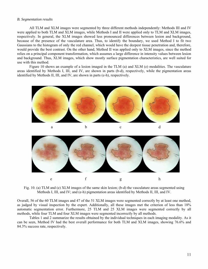
B. Segmentation results All TLM and XLM images were segmented by three different methods independently: Methods III and IV were applied to both TLM and XLM images, while Methods I and II were applied only to TLM and XLM images, respectively. In general, the XLM images showed less pronounced differences between lesion and background, because of the presence of the vasculature area. Thus, to identify the boundary, we used Method I to fit two Gaussians to the histogram of only the red channel, which would have the deepest tissue penetration and, therefore, would provide the best contrast. On the other hand, Method II was applied only to XLM images, since the method relies on a principal component transformation, which assumes a large difference in intensity values between lesion and background. Thus, XLM images, which show mostly surface pigmentation characteristics, are well suited for use with this method.

Figure 10 shows an example of a lesion imaged in the TLM (a) and XLM (e) modalities. The vasculature areas identified by Methods I, III, and IV, are shown in parts (b-d), respectively, while the pigmentation areas identified by Methods II, III, and IV, are shown in parts (e-h), respectively.

d b c a

h f g e

Fig. 10. (a) TLM and (e) XLM images of the same skin lesion; (b-d) the vasculature areas segmented using Methods I, III, and IV; and (e-h) pigmentation areas identified by Methods II, III, and IV.

Overall, 56 of the 60 TLM images and 47 of the 51 XLM images were segmented correctly by at least one method, as judged by visual inspection by the expert. Additionally, all these images met the criterion of less than 18% automatic segmentation error. Furthermore, 25 TLM and 25 XLM images were segmented correctly by all methods, while four TLM and four XLM images were segmented incorrectly by all methods.

Tables 1 and 2 summarize the results obtained by the individual techniques in each imaging modality. As it can be seen, Method IV had the best overall performance for both TLM and XLM images, showing 76.6% and 84.3% success rate, respectively.

11

Table 1. Segmentation results for TLM images.

Method I Method III Method IV Correctly segmented TLM images 41 45 46 Total number of images 60 60 60 Success Rate 68.3% 75.0% 76.6%

Table 2. Segmentation results for XLM images.

Method I Method II Method IV Correctly segmented XLM images 35 40 43 Total number of images 51 51 51 Success Rate 68.6% 78.4% 84.3%

C. Scoring Stage

After segmenting the TLM and XLM images individually, the scoring stage selected one of the three segmented images as the final result, based on the set of criteria mentioned earlier. In all cases in which at least one method gave correct results, the scoring stage was able to select the correct answer. Figure 11 shows an example in which only one method achieved correct segmentation of a TLM image, while the other two failed; yet, the scoring stage was able to select the correct segmentation as the final result.

Selection Rules

(a) (b) (c)

(a)

Selection Rules

(b) (c)

(a)

Scoring System

(b) (c)

(a)

Selection Rules

(b) (c)

(a)

Selection Rules

(b) (c)

(a)

Scoring System

(b) (c)

(a)

Selection Rules

(a) (b) (c)

(a)

Selection Rules

(b) (c)

(a)

Scoring System

(b) (c)

(a)

Selection Rules

(b) (c)

(a)

Selection Rules

(b) (c)

(a)

Scoring System

(b) (c)

(a)

Fig. 11. Example of a TLM image segmented with three different methods (top row), and final result selected by the scoring stage (bottom).

12

The usefulness of the scoring stage is summarized in Table 3, which shows that the overall performance of the system that includes the scoring stage was increased to 93.3% and 92.2%, for the XLM and TLM images, respectively, providing a 21.6% and 9.3% net improvement, respectively.

Table 3. Performance of the scoring stage.

TLM images XLM images Total number of lesions 60 51 Number of lesion where all the segmentation techniques failed

4 4

Number of lesions where at least one segmentation technique gave correct results

56 47

D. Validation of segmentation results

The system performance was quantified by computing a percent error between automatic and manual segmentation, separately for each image, in each imaging modality. An example of automatic and manual segmentation of a TLM image is shown on the left and right panels of Figure 12, respectively.

Fig. 12. Example of automatic (left) and manual (right) segmentation of a lesion.

The average error was also computed for the images correctly segmented by all methods and for the final

result image selected by the scoring system. These results are summarized in Table 4, where it can be seen that the two-stage system had a lower error ratio than each individual method, in both imaging modalities.

Table 4. Average error ratio for each segmentation method and the scoring stage in each imaging modality.

Method I Method II Method III Method IV Scoring Stage TLM modality. 24% – 19.4% 16.5% 14% XLM modality. – 18.8% 16.5% 15.3% 15.1%

13

14

E. Malignancy detection A total of 40 lesions that had both the TLM and XLM images correctly segmented by the automatic

procedures were further analyzed for assessing malignancy. The lesions were categorized as Benign, Compound Nevi, Dysplastic Nevi, or Melanomas, based on data from pathology. Table 5 summarizes for each lesion the TLM and XLM area measurements, the TLM/XLM ratio, the percent TLM area change, the exact description of the lesion by the dermatologist, and the final lesion classification by pathology.

Table 5. Area difference across the TLM and XLM modalities for various types of skin lesions.

Lesion ID TLM Area XLM area TLM/XLM %∆A Pathology Classification

Lesion Type

1 581 684 0.849 -17.73 Benign Lentigo Benign 2 9188 8278 1.110 9.90 Dysplastic nevus Malignant 3 10507 7930 1.325 24.53 Malignant Melanoma Malignant 4 23540 13755 1.711 41.57 Malignant Melanoma Malignant 5 3303 2055 1.607 37.78 Mod dysplastic nevus Malignant 9 2708 2950 0.918 -8.94 Seborrheic Keratosis Benign

10 2144 2200 0.975 -2.61 Intradermal nevus Benign 11 1991 1500 1.327 24.66 Dysplastic nevus Malignant 15 3037 3268 0.929 -7.61 Compound nevus X 17 5015 4718 1.063 5.92 Seborrheic Keratosis Benign 20 6850 7153 0.958 -4.42 Seborrheic Keratosis Benign 22 2235 1791 1.248 19.87 Dysplastic nevus Malignant 25 1450 1693 0.856 -16.76 Junctional nevus Benign 27 2880 2654 1.085 7.85 Intradermal congenital Benign 28 3365 2433 1.383 27.70 Compound nevus X 29 1620 1456 1.113 10.12 Junctional nevus Benign 32 5395 4183 1.290 22.47 Compound nevus X 33 6252 4958 1.261 20.70 Compound nevus X 49 4761 4297 1.108 9.75 Compound nevus X 57 4142 3408 1.215 17.72 Dyspl. Comp. nevus Malignant 59 8571 8349 1.027 2.59 Benign Benign 61 1595 1351 1.181 15.30 Compound nevus X 62 2412 2216 1.088 8.13 Compound nevus X 64 4380 3048 1.437 30.41 Compound nevus X 65 2497 3035 0.823 -21.55 Compound nevus X 67 1509 2000 0.755 -32.54 Intradermal nevus Benign 70 7284 7560 0.963 -3.79 Dysplastic nevus Malignant 73 1938 1197 1.619 38.24 Dysplastic nevus Malignant 78 2323 1964 1.183 15.45 Junctional nevus Benign 79 4175 3595 1.161 13.89 Seborrheic Keratosis Benign 81 7431 6278 1.184 15.52 Compound nevus X 87 5215 4262 1.224 18.27 Intradermal nevus Benign 92 2986 2455 1.216 17.78 Dysplastic nevus Malignant 94 7338 4499 1.631 38.69 Data not available X 95 5498 4767 1.153 13.30 Data not available X

104 7041 6507 1.082 7.58 Data not available X 106 4960 4714 1.052 4.96 Data not available X 107 12609 10746 1.173 14.78 Data not available X 108 13008 10569 1.231 18.75 Data not available X

Typically, the malignant lesions show a much larger area in the XLM image that corresponds to blood vessels

developed to support the growing cancer, while the benign lesions show approximately the same area in both images. Figure 13 shows the difference between a malignant and a benign lesion in the TLM and XLM imaging modalities. The lesions in the upper row represent a mild dysplastic nevus, while the images in the lower row correspond to a compound nevus.

Fig. 13. TLM (left column) and XLM (right column) images of benign (upper row) and malignant (lower row) lesions. Notice the increase in area in the malignant lesion.

The average values of the ratio between the TLM and XLM areas and the percent change in area when only

lesions with results confirmed by pathology are used are summarized in Table 6, which shows clear mean differences between benign, malignant and, dysplastic nevi. Thus the area difference can be use as a criterion for malignancy.

Table 6. Average increase in TLM area of the skin lesions categorized by lesion type.

Benign Lesions Dysplastic Nevi Malignant Lesions TLM/XLM 1.01 1.17 1.33

%∆A -0.69 0.19 0.24

If the lesions without pathology results are ignored, and excluding the dysplastic nevi which can become either malignant or benign, the remaining 23 lesions are either malignant or benign. In this case, a simple threshold for the %∆A parameter at 1.2 can separate almost all benign lesions from the malignant ones. More specifically, the 23 lesions classified as shown in the confusion matrix reported in Table 7, which shows a sensitivity of 80%, specificity of 92.3%, and an overall accuracy of 86.9% in determining the malignancy of a lesion.

Table 7. Overall performance of the system. 15

16

Predicted Malignant Benign

Malignant 8 (True Positive) 2 (False Positive) Actual Benign 1 (False Negative) 12 (True Negative)

IV. CONCLUSIONS AND DISCUSSION Skin cancer is the most common of all cancers and represents about one half of all new cancers detected. Approximately 1.2 million new cases of skin cancer are being detected in the United States each year. About 80% of all skin cancers are basal cell carcinomas, 16% are squamous cell carcinomas, and 4% are melanomas. Melanoma is the deadliest of the skin cancers, accounting for over 7300 cancer deaths per year in the United States. The incidence of melanoma in the United States increased by 3% between 1997 and 1998 and approximately 44,200 new cases of malignant melanoma were detected in 1999 [1]. Early detection of skin cancer is of paramount importance. If detected at an early stage, skin cancer has one of the highest cure rates, and in most cases, the treatment is quite simple and involves excision of the lesion. Moreover, at an early stage, skin cancers are very economical to treat, while at a late stage, cancerous lesions usually result in near fatal consequences and have a extremely high costs associated with the necessary treatment. For example, melanomas, the deadliest form of all skin cancers, account for 75% of all cancer deaths [1-4]; however, when detected at an early stage, the cure rate is higher than 95%.

We have developed a methodology that can automatically segment a lesion and accurately measure both the pigmentation and vasculature related characteristics. Independently, the success rate of correct segmentation of each of these techniques is in the order of 75%, but the additional stage that combines results from all three methods and a set of ad hoc criteria increased the success rate to 95%. Our approach can have a significant impact in the field of cancer research. More specifically, our procedures can result beneficial to the patients that undergo screening by replacing the current imaging procedures, which are inherently limited and liable to subjective interpretation, with an automatic and unbiased approach that extracts the maximum amount of information from a lesion and helps the physician make a correct diagnosis. This can result in a more accurate diagnosis, safer surgical treatment, improved quality of life for the patients, and at the same time decreases the cost of health care delivery. These results provide strong support for using transillumination imaging in the early diagnosis of skin cancer.

REFERENCES [1] Abidi M. and Gonzales R., Eds., “Data Fusion in Robotics and Machine Intelligence”, New York Academic, 1992. [2] Alexander A., Nazarian N. M., Capuzzi D. M., Rawool N. M., Kurtz A. B., and Mastrangelo M.J., “Color Doppler

sonography detection of tumor flow in superficial melanoma metastases: histologic correlation”, J. Ultrasound Med., vol. 17, 123-126, 1998.

[3] Anonymous authors, “American Cancer Association and the American Academy of Dermatology”, Web publications, 2001.

[4] Binder M., Schwarz M., Winkler A., Steiner A., Kaider A., Wolff K., and Pehamberger H., “Epiluminescence Microscopy. A useful tool for the diagnosis of pigmented lesions for formally trained dermatologists”, Arch. Dermatology, vol. 131, 286-291, 1995.

[5] Binder M., “Skin Examination Device”, US Patent Number 6,032,071, Published in 2000. [6] Bischof L., Talbot H., Breen E., Lovell D., Chan D., Stone G., Menzies S., Gutenev A., and Caffin R., “An Automated

Melanoma Diagnosis System”, New Approaches in Med. Image Analysis, SPIE, vol. 3747, 130-141, 1999. [7] Brochez L., Verhaeghe E., Bleyen L., and Naeyaert J. M., “Diagnostic ability of general practitioners and dermatologists

in discriminating pigmented skin lesions”, J. Am Acad. Dermatology, vol. 44, 976-86, 2001. [8] Cancer facts and figures 2002, “American cancer society”, Atlanta, Georgia, 2002. [9] Claridge E., Hall P. N., Keefe M., and Allen J. P., “Shape analysis for classification of malignant melanomas”, J.

Biomed. Eng., vol. 16, no. 3, 191-197, 1992. [10] DeCoste S. D., and Stern R. S., “Diagnosis and treatment of nevomelanocytic lesions of the skin. A community based

study”, Arch. of Dermatology, vol. 129, no. 1, 57-62, 1993. [11] Detmar M., “Tumor angiogenesis”, J. Investig. Dermatology Symp. Proc., vol. 5, 20-23, 2000.

17

[12] Dhawan A. P., Gordon R., and Rangayyan R. M., “Nevoscopy: Three-dimensional computed tomography for nevy and melanoma by side-transillumination”, IEEE Trans. in Med. Imaging, MI-3, 54-61, 1984.

[13] Dhawan A. P., “Apparatus and method for skin lesion examination”, US Patent Number 5,146,923, 1992. [14] Dhawan, A. P., Gordon R., and Rangayyan R. M., “Computed tomography by side-transillumination to detect early

melanoma”, IEEE Annual Conf. Proc. of Eng. in Med., 518-522, 1984. [15] Dhawan A. P. and Sicsu A., “Segmentation of images of skin lesions using color and texture information of surface

pigmentation”, Computerized Med. Imaging and Graphics, vol. 16, no. 3, 163-177, 1992. [16] Doshi M., Duvic M., Mullani N., and Zouridakis G., “Early diagnosis of skin cancer based on measuring vascularization

and pigmentation in Nevoscope images”. Abstracts of the Annual Houston Conf. on Biomed. Eng., 2004. [17] Duda R., Hart P. and Stork D. “Pattern Classification”, Wiley Publication, second edition, 2000. [18] Ganster H., Pinz A., Rohrer R., Wildling E., Binder M., and Kittler H., “Automated Melanoma Recognition”, IEEE

Trans. on Med. Imaging, vol. 20, no. 3, 233-239, 2001. [19] Gee M. S., Saunders H. M., Lee J. C., Sanzo J. F., Jenkins W. T., Evans S. M., Trinchieri G., Sehgal C. M., Felman M.

D., and Lee W. M., “Doppler ultrasound imaging detects changes in tumor perfusion during antivascular therapy associated with vascular anatomic alterations”, Cancer research, vol. 61, 2974-2982, 2001.

[20] Giovagnorio F., Andreoli C., and De Cicco M. L., “Color doppler sonography of focal lesion of the skin and subcutaneous tissue”, J. Ultrasound Med., vol. 18, 89-93, 1999.

[21] Gloster H. M., and Brodland D. G., “The epidemiology of skin cancer”, Dermatology Surg., vol. 22, 217-226, 1996. [22] Goldsmith L. A, Koh H. K, Bewerse B. A., Reilley B., Wyatt S.W., Bergfeld W.F., Geller A.C., and Walters P. F.,

“Proceedings from the national conference to develop skin cancer agenda ”, CDC 1995. [23] Goshtasby A., “Fitting Parametric Curves to Dense and Noisy Points”, Presented at 4th Int’l Conf. Curves and Surfaces,

1999. [24] Green A., Martin N., Pfitzner J., O’Rouke M., and Knight N., “Computer image analysis in the diagnosis of melanoma”,

J. American Acad. of dermatology, vol. 31, no. 6, 958-964, 1994. [25] Hance G. A., and Umbaugh S. E., Moss R. H., and Stoecker W. V., “Unsupervised color image segmentation”, IEEE

Eng. Med. Biol. Mag., vol. 15, no. 1, 104-111, 1996. [26] Kelly J. W., Yeatman J. M., Regalia C., Mason G., Henham A. P., “A high incidence of melanoma found in patients

with multiple dysplastic nevi by photographic surveillance”, MJA, vol. 167, no. 4, 191-194, 1997. [27] Mullani N. A., Talpur R., Apisarnthanarax N., Weinstock M., Drugge R., Ahn C., Prieto V. G., and Duvic M., “Side-

transillumination epiluminescence imaging for diagnosis of dysplastic nevi and melanoma. A comparison to oil and cross-polarization epiluminescence imaging”, in press.

[28] Nachbar F., Stolz W., Merkle T., Cognetta A. B., Vogt T., Landthaler M., Bilek P., Braun-Falco O., and Plewig G., “The ABCD rule of dermatoscopy. High prospective value in the diagnosis of doubtful melanocytic skin lesions”, J. Am Acad. of Dermatology, vol. 30, no. 4, 551-559, 1994.

[29] Nevoscope web site at www.nevoscope.com. [30] Otsu N., “A Threshold Selection Method from Gray-Level Histograms”, IEEE Trans on Systems, Man, and

Cybernetics, vol. 9, no. 1, pp. 62-66, 1979. [31] Pehamberger H., Steiner A., and Wolff K., “In vivo epiluminescence microscopy of pigmented skin lesions. I. Pattern

analysis of pigmented skin lesions”, J. Am Acad. Dermatology, vol. 17, no. 4, 571-583, 1987. [32] Perelman R.O., “An estimate of the incidence of malignant melanoma in the United States. Based on a survey of

members of the American Academy of Dermatology”, Dermatologic Surgery, vol. 21, no. 4, 301-305, 1995. [33] Roberts M. E. and Claridge E., “An artificially evolved vision system for segmenting skin lesion images”, MICCAI,

LNCS 2878, 655-662, 2003. [34] Sonka M., Hlavac V., and Boyle R., “Image processing, analysis, and machine vision”, Brooks Cole, Second edition,

1998. [35] Stolz W., Riemann A., Przetak C., Bilek P., Landthaler M., Braun-Falco O., Holzel D., and Abmayr W. “Multivariate

analysis of criteria given by dermatoscopy for the recognition of melanocytic lesions”, Book of Abstracts, Am Acad. of Dermatology Meeting, Dallas, 53, 1991.

[36] Tur E., and Brenner S., “Cutaneous blood flow measurement for the detection of malignancy in pigmented lesions”, J. Dermatology, vol. 184, no. 1, 8-11, 1992.

[37] Umbaugh S. E., Moss R. H., Stoecker W. V., and Hance G. A., “Automatic color segmentation algorithms: With application to skin tumor feature identification”, IEEE Eng. Med. Biol. Mag., vol. 12, no. 3, 75-82, 1993.

[38] Umbaugh S. E., Moss R. H., and Stoecker W. V., “An automatic segmentation algorithm with application to identification of skin tumor borders”, Comp. Med. Imaging and Graphics, vol.16, no. 3, 227-235, 1992.

[39] Umbaugh S. E., Moss R. H., and Stoecker W. V., “Automatic color segmentation of images with application in detection of variegated coloring in skin tumors”, IEEE Eng. Med. Biol., vol. 8, 43-52, 1989.

[40] Wolff K., Binder, and M., Pehamberger H., “Epiluminescence microscopy: a new approach to the early detection of melanoma”, Adv in Dermatology, vol. 9, 45-56, 1994.

[41] Xu L., Jackowski M., Goshtasby A., Roseman D., Bines S., Yu C., Dhawan A., and Huntley A., “Segmentation of skin cancer images”, Image and Vision Computing, vol. 17, 65-74, 1999.

18

[42] Zharkova V.V., Ipson S. S., Zharkov S. I., Benkhalil A. K., Aboudarham J., and Bentley R. D., “A full disk image standardisation of the synoptic solar observations at the Meudon observatory”, J. Solar Physics, vol. 214, no. 1, 89-105, 2003.

[43] http://rsb.info.nih.gov/nih-image/about.html. [44] http://edcenter.med.cornell.edu/CUMC_PathNotes/Dermpath/Dermpath_07.html. [45] http://www.bccancer.bc.ca/HPI/CME/SkinCancer/CMESkinCancer/Readings/Prevention/

DysplasticNevus.htm. [46] http://mathworld.wolfram.com/FullWidthatHalfMaximum.html [47] Shankar A. Automatic Segmentation of PET Images and Volumetric Measurement of Metabolic Activity, MS Thesis,

University of Houston, 2004. [48] Doshi M. Automatic Segmentation of Skin Cancer Images, MS Thesis, University of Houston, 2004.