Transient Hot Wire Apparatus – Standard Operating Procedure (SOP) For

Thermal Conductivity Measurements of Non-Flammable Liquid Mixtures

2020

Table of Contents

Experimental overview ..................................................................................................................... 3

Basic principles .................................................................................................................................... 4

Reference Readings ............................................................................................................................ 4

Equipment .............................................................................................................................................. 5

Safety ........................................................................................................................................................ 6

Risk Summary .................................................................................................................................................. 6 Emergency Shutdown .................................................................................................................................... 7 Reporting and Duty of Care ......................................................................................................................... 7

Experimental Process ........................................................................................................................ 7

Preparation and filling the system with sample gas or gas mixtures .................................................... 8 Measurement of thermal conductivity ............................................................................................................... 9 Completion / switch to another gas ................................................................................................................. 13

Troubleshooting ................................................................................................................................ 14

Leaks ................................................................................................................................................................. 14 Software and data recording guide ........................................................................................................ 14

Labview software ..................................................................................................................................................... 14 Data recording spreadsheet ................................................................................................................................. 20 Data output files ........................................................................................................................................................ 23

Experimental overview In this work, transient hot-wire method is used to measure the thermal conductivity of gas and gas mixtures. Two 25 μm diameter anodized tantalum wires of length 57.7 mm and 27.0 mm were arranged in opposite arms of a Wheatstone bridge in order to eliminate the end effects arising from axial conduction. The data acquisition system (capable of multi-channel sampling at 1 MHz) interrogated several voltages in the circuit simultaneously. The pressure transducer and two platinum resistance thermometer have been calibrated before the measurement, and the resistances of the two tantalum wires have been determined as a function of temperature. A custom Labview program can be used to analyse and record data automatically. The output data should be further processed in an analysis spreadsheet

V4

Bath

Cell V6

PT

V1V2

Vacuum Pump

Drain

V5PRT

PRT

V3

Jacket

Isco Pump 1

Gas Cylinder

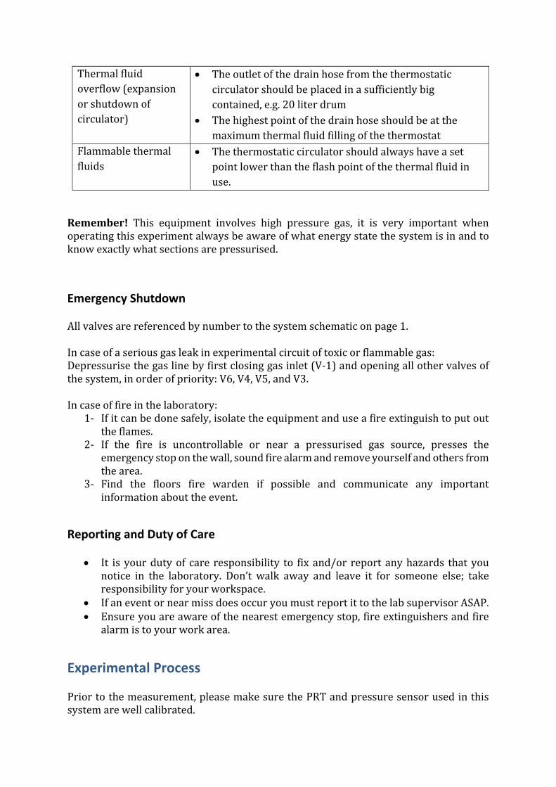
Figure 1. Simplified schematic of transient hot-wire apparatus.

Figure 1 provides a picture of our system which showing the main parts of the apparatus.

Basic principles Ideally, the thermal conductivity of the fluid is determined by observing the rate at which the temperature of a very thin metallic wire increases with time, after a step change in voltage has been applied to it, thus creating in the fluid a line source of essentially constant heat flux per unit length. The wire acts as a) heat source, but also as b) resistance thermometer The fundamental working equation of the transient hot-wire method takes the form:

(1) and it gives the possibility to obtain the thermal conductivity of the measured material from the slope of the line ΔT versus lnt. In the above equation q is the power input per unit length of wire, λ is the thermal conductivity of the fluid at certain temperature T and pressure p. ro is the wire radius, t the time, α is the constant thermal diffusivity, and γ is the Euler constant equal to 0.5772157. In practice, the design of the experimental setup for the measurement of the thermal conductivity of a material introduces a number of departures from the ideal solution. Therefore, essential corrections have to be made to the acquired experimental data to adjust it to the ideal model described by equation (1). The corrections applied to the experimentally measured temperature rise follow the equation

(2) where ΔTid(ro,t) is the ideal temperature rise at the wire radius ro at time t, ΔΤexp(t) is the temperature rise measured experimentally and ΣiδTi is a sum of the applied corrections. The corrections to the ideal solution have been presented explicitly elsewhere [3]- [10].

Reference Readings [1] Roder, H. M., A transient hot wire thermal conductivity apparatus for fluids. J. Res.

Natl. Bur. Stand 1981, 86 (5), 457-493. [2] Degroot, J. J.; Kestin, J.; Sookiazi.H, INSTRUMENT TO MEASURE THERMAL-

CONDUCTIVITY OF GASES. Physica 1974, 75 (3), 454-482.

[3] Healy, J. J.; Degroot, J. J.; Kestin, J., THEORY OF TRANSIENT HOT-WIRE METHOD FOR MEASURING THERMAL-CONDUCTIVITY. Physica B & C 1976, 82 (2), 392-408.

[4] Degroot, J. J.; Kestin, J.; Sookiazi.H, INSTRUMENT TO MEASURE THERMAL-CONDUCTIVITY OF GASES. Physica 1974, 75 (3), 454-482.

[5] Healy, J. J.; Degroot, J. J.; Kestin, J., THEORY OF TRANSIENT HOT-WIRE METHOD FOR MEASURING THERMAL-CONDUCTIVITY. Physica B & C 1976, 82 (2), 392-408.

[6] Mason, E. A.; Khalifa, H. E.; Kestin, J.; Dipippo, R.; Dorfman, J. R., COMPOSITION DEPENDENCE OF THERMAL-CONDUCTIVITY OF DENSE GAS-MIXTURES. Physica A 1978, 91 (3-4), 377-392.

[7] Moroe, S.; Woodfield, P. L.; Fukai, J.; Shinzato, K.; Kohno, M.; Fujii, M.; Takata, Y., THERMAL CONDUCTIVITY MEASUREMENT OF GASES BY THE TRANSIENT SHORT-HOT-WIRE METHOD. Experimental Heat Transfer 2011, 24 (2), 168-178.

[8] Moroe, S.; Woodfield, P. L.; Kimura, K.; Kohno, M.; Fukai, J.; Fujii, M.; Shinzato, K.; Takata, Y., Measurements of Hydrogen Thermal Conductivity at High Pressure and High Temperature. International Journal of Thermophysics 2011, 32 (9), 1887-1917.

[9] Woodfield, P. L.; Moroe, S.; Fukai, J.; Fujii, M.; Shinzato, K.; Kohno, M.; Takata, Y., Techniques for Accurate Resistance Measurement in the Transient Short-Hot-Wire Method Applied to High Thermal-Diffusivity Gas. International Journal of Thermophysics 2009, 30 (6), 1748-1772.

[10] Kestin, J., & Wakeham, W. A., 1978, “A contribution to the theory of the transient hot-wire technique for thermal conductivity measurements”, Physica A: Statistical Mechanics and its Applications, 92: 102-116.

Equipment This equipment list does include some elements that are no longer in use in the current set up but have been included for reference. Table 1: List of apparatus equipment

Equipment Description ISCO Pump ISCO 260 D Syringe Pump Thermostatic Circulator Lauda RPT 1290, (-88 to 200) °C Keller PAA 33X Pressure transmitter, (0 – 300 bara) Agilent E3648A DC power supply DC regulated power supply 0 – 30 V, 0 – 3 A Resistance Box * 4 CROPICO, Type RBB6-B Reference resistor NI BNC-2120 BNC Terminal Blocks NI PCIe-6361 DAQ board, in computer Agilent 34410A * 2 Digit multimeter Custom electric board Switch and Wheatstone bridge Custom pressure vessel Made of 17-4PH Burst disk / holder HIP burst disk holder, burst disk 4200 PSI

Fittings and Valves HiP Taper Seal Range and Swagelok Tubing 1/4, 1/8 and 1/16 316 SS Bath Custom made with heating / cooling jacket Stirrer Flat plate, driven by electric engine of

unknown brand Bath lid Lid with all tubing, stirrer, pressure

transmitter Hoses between bath and thermostat Insulation Cryogel as well as cellular rubber

Safety

Risk Summary The following table should only be used as a general overview of the hazards associated with this experiment. Prior to commencing any work with this apparatus persons should be familiar with the formal risk assessment and safety management plans, which can be found on the network here \\drive.irds.uwa.edu.au\MECH-FD-001\Projects\CO2 Research\01 CO2-CH4 Dispersion\09 - Safety These routines have not been developed with test of flammable or toxic fluids / gases in mind. If this is relevant, routines should be reviewed and probably new measures introduced.

Hazards Controls Flammable gases • No naked ignition sources allowed in lab.

• Small volumes of flammable gas. High Pressure liquids /gas

• Safety glasses and laboratory coat • SOP for pressurising/depressurising circuit • Small volumes of gas.

Slips and trips • Maintain tidy work area. Other experiments in vicinity

• Respect others workspace. • Communicate clearly with others intentions in lab space.

Water + Electricals • Tighten water lines securely and double check for leaks. Manual handling (especially core holder)

• Proper technique. • Take time to assess task. • Ask for assistance when required

High strength magnetic field

• Do not place sensitive equipment or cards near magnet.

Thermal fluid overflow (expansion or shutdown of circulator)

• The outlet of the drain hose from the thermostatic circulator should be placed in a sufficiently big contained, e.g. 20 liter drum

• The highest point of the drain hose should be at the maximum thermal fluid filling of the thermostat

Flammable thermal fluids

• The thermostatic circulator should always have a set point lower than the flash point of the thermal fluid in use.

Remember! This equipment involves high pressure gas, it is very important when operating this experiment always be aware of what energy state the system is in and to know exactly what sections are pressurised.

Emergency Shutdown All valves are referenced by number to the system schematic on page 1. In case of a serious gas leak in experimental circuit of toxic or flammable gas: Depressurise the gas line by first closing gas inlet (V-1) and opening all other valves of the system, in order of priority: V6, V4, V5, and V3. In case of fire in the laboratory:

1- If it can be done safely, isolate the equipment and use a fire extinguish to put out the flames.

2- If the fire is uncontrollable or near a pressurised gas source, presses the emergency stop on the wall, sound fire alarm and remove yourself and others from the area.

3- Find the floors fire warden if possible and communicate any important information about the event.

Reporting and Duty of Care

• It is your duty of care responsibility to fix and/or report any hazards that you notice in the laboratory. Don’t walk away and leave it for someone else; take responsibility for your workspace.

• If an event or near miss does occur you must report it to the lab supervisor ASAP. • Ensure you are aware of the nearest emergency stop, fire extinguishers and fire

alarm is to your work area.

Experimental Process Prior to the measurement, please make sure the PRT and pressure sensor used in this system are well calibrated.

Preparation and filling the system with sample gas or gas mixtures This routine is optimized for mixtures, and to minimize the impact of any phase separation of the pressure transmitter by ensuring a one-way flow in the long line between the cell and V6. 1. Before starting to use the system for a while, conduct pressure test of pressure vessel

and pipeline to the highest pressure of the measurement. Test leaking with Sloop (liquid leak detector) or with the leak detector device and pressure sensor.

2. Connect the gas to be investigated to the isco-pump via V1 3. Evacuate the whole system:

a. Make sure that none of the volumes to be evacuated are pressurized above 1.5 bara

b. Start the vacuum pump with all valves closed c. Open valves successively V2 – V4 – V3 – V1 -V5. d. Run the vacuum pump for enough time to the pressure has stabilized. Longer

time is required if used with dissimilar components, liquids, or the system has not been used in a while. Start evacuation with the pump at minimum volume position.

e. Charging of the system can now start 4. Parallel with the evacuation, complete mixture of the gas cylinder content shall be

assured by heating the bottom part of the cylinder using a heat belt. a. The set-point of the heat belt should be 70 unless that is deemed unsafe due to

pressure increase b. the heating should run 24 hours prior to filling the cell. c. Especially long mixing time is required if there is a suspicion of phase

separation during filling or storage. d. Leave the heating on until the charging of the cell is completed. Longer if test

mixture should be used in another experiment and it is suspected that the storage condition may lead to phase separation.

5. When thermal conductivity shall be found for a mixture, make sure that the pump and cell at supercritical temperature with a margin of at least 10 °C before injecting any fluids into the system, but the cell shall never be above the flash point of the thermal fluid under used.

6. In some cases flushing may be advisable. Perform flushing by: a. Close all valves b. Have a small volume of the ISCO pump c. Open valves V1 and V3 and the gas cylinder valve and fill the ISCO pump d. Close the gas cylinder valve, and sett the ISCO pump to the desired flushing

pressure. i. Flush the system before the cell by disconnecting the vacuum pump,

open valve V4 and very careful open V2 and slowly let the pressure down to 1.5 bar (note that the ISCO-pump shows higher than actual pressure)

ii. OR flush the whole system by open valve V4, very carefully open V5 until the system pressure has equalized, and very carefully open valve V6 and reduce system pressure slowly to 1.5 bar.

e. Evacuate the flushed part of the system 7. Open valves V1 and V3, and refill the ISCO pump 8. Close V1 and V3 and cylinder valve

9. If charging a mixture and the temperature of the tubing leading to the cell is below supercritical temperature, ensure that the pressure of the ISCO-pump is well above the cricondenbar

10. Open V4 11. Carefully open V5 slightly. Too high flow may break the tantalum wires 12. Set the flow limit of the ISCO pump at 15 ml/minute, and observe the flow. If the flow

is 15 ml/minute while the pump pressure is decreasing or stable, reduce valve V5 opening at once as the flow is too high. Make sure that the pressure in the pump is always supercritical if injecting a mixture with cricondentherm similar or higher than the room temperature

13. If the cell is at the pump pressure, V5 can be opened fully. 14. Set the first target pressure of the ISCO pump to the first test pressure, which should

be at a supercritical pressure 15. Use the pressure constant mode of ISCO pump to pressurize the cell 16. If the ISCO pump becomes close to empty and the cell pressure is still below the

cricondenbar, close V5 right before the pump becomes empty to avoid depressurization of the line leading to the cell.

17. If the set point pressure of the ISCO pump cannot be reached in the, V4 and V5, otherwise go to step18

a. Refill the ISCO pump b. Open V3, V1, and the gas cylinder valve. Close these valves when the pump

pressure has stabilized c. Set the ISCO pump pressure equal to the cell pressure d. Go to step 6

18. If going below freezing temperatures, make sure to avoid ice formation in the burst disk tube by sealing it with a tape or similar, or attach a long tube.

19. Set the temperature of the bath to the lowest test pressure 20. When the temperature of the cell has stabilized for 2 hours, close V4 and V5 21. Perform measurement of thermal conductivity (see below) 22. Go to the next lower pressure by very carefully open V6 slightly 23. Going to the next higher temperature point will increase the pressure dramatically

when working with liquids: a. Be sure to check that the pressure of the vessel is always 20 % below the burst

disk pressure by estimating the impact of thermal expansion. b. Add intermediate temperature steps if needed, and open V6 slightly to reduce

pressure before increasing temperature further

Measurement of thermal conductivity 1. Test the resistance of both long wire and short wire to make sure the wires are

not broken and well connected. 2. Check if any of the wires is touching the pressure vessel. If you notice any

resistance between the wires and the cell you have to open the cell and check your sensor.

3. Check settings for hardware. a) DC regulated power supply: 15 V, supply voltage to the switch of custom

electronic board. b) The light on the BNC-2120 is on.

4. Turn on the Agilent E3648A DC Power Supply. a) Press the Output On/Off button.

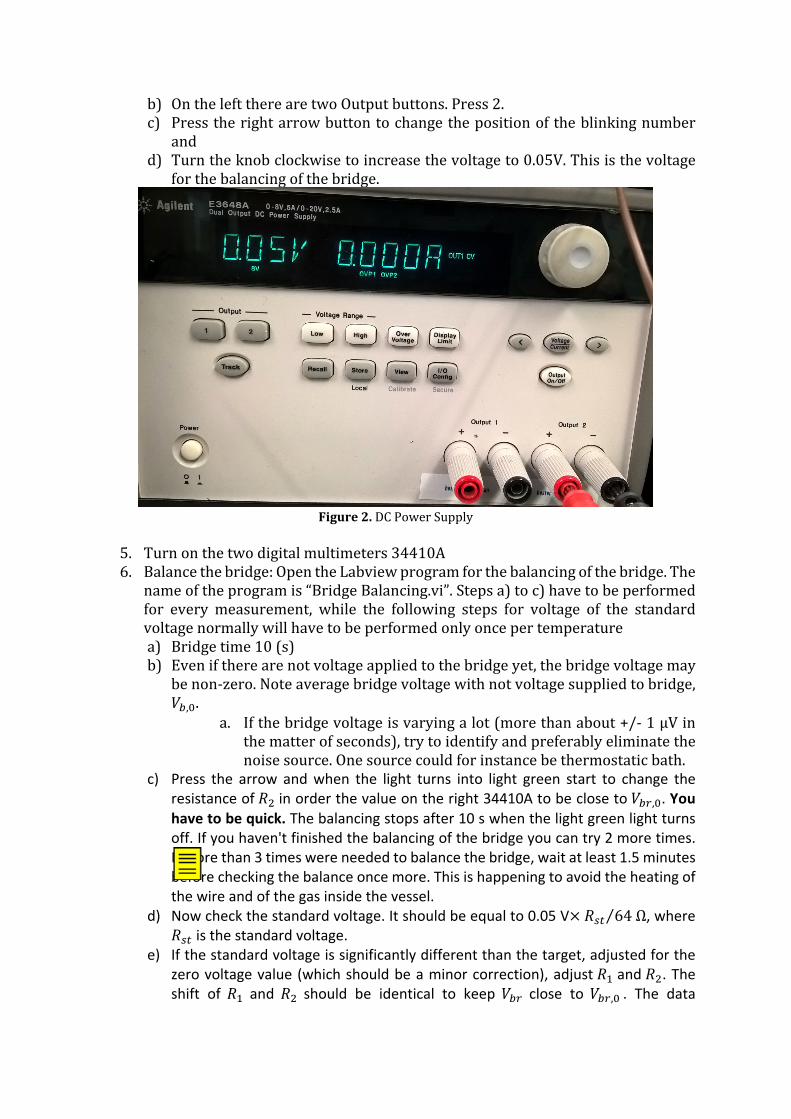
b) On the left there are two Output buttons. Press 2. c) Press the right arrow button to change the position of the blinking number

and d) Turn the knob clockwise to increase the voltage to 0.05V. This is the voltage

for the balancing of the bridge.

Figure 2. DC Power Supply

5. Turn on the two digital multimeters 34410A 6. Balance the bridge: Open the Labview program for the balancing of the bridge. The

name of the program is “Bridge Balancing.vi”. Steps a) to c) have to be performed for every measurement, while the following steps for voltage of the standard voltage normally will have to be performed only once per temperature a) Bridge time 10 (s) b) Even if there are not voltage applied to the bridge yet, the bridge voltage may

be non-zero. Note average bridge voltage with not voltage supplied to bridge, 𝑉𝑉𝑏𝑏,0.

a. If the bridge voltage is varying a lot (more than about +/- 1 µV in the matter of seconds), try to identify and preferably eliminate the noise source. One source could for instance be thermostatic bath.

c) Press the arrow and when the light turns into light green start to change the resistance of 𝑅𝑅2 in order the value on the right 34410A to be close to 𝑉𝑉𝑏𝑏𝑏𝑏,0. You have to be quick. The balancing stops after 10 s when the light green light turns off. If you haven't finished the balancing of the bridge you can try 2 more times. If more than 3 times were needed to balance the bridge, wait at least 1.5 minutes before checking the balance once more. This is happening to avoid the heating of the wire and of the gas inside the vessel.

d) Now check the standard voltage. It should be equal to 0.05 V× 𝑅𝑅𝑠𝑠𝑠𝑠 64 Ω⁄ , where 𝑅𝑅𝑠𝑠𝑠𝑠 is the standard voltage.

e) If the standard voltage is significantly different than the target, adjusted for the zero voltage value (which should be a minor correction), adjust 𝑅𝑅1 and 𝑅𝑅2. The shift of 𝑅𝑅1 and 𝑅𝑅2 should be identical to keep 𝑉𝑉𝑏𝑏𝑏𝑏 close to 𝑉𝑉𝑏𝑏𝑏𝑏,0 . The data

reporting spreadsheet to be described below provides an aid to set the new values of 𝑅𝑅1 and 𝑅𝑅2

f) If the shift of 𝑅𝑅1 and 𝑅𝑅2 has been equal, the bridge should be still close to balanced, but nevertheless repeat step b)-e) until the bridge is fully balanced.

g) When the bridge is fully balanced, not the value of 𝑅𝑅1 in the data recording spreadsheet

7. Set the source voltage to 𝑉𝑉𝑠𝑠 = 0 V, and run the bridge balancing labview application once more. Observe the varying value of the measurement of 𝑉𝑉𝑠𝑠𝑠𝑠 and note the approximate minimum and maximum values. Record the mean value and the maximum deviation from this value in the data recording spreadsheet

8. Change the source voltage 𝑉𝑉𝑠𝑠to a value that will provide an estimated temperature increase of about 2 °C, typically between 0.70-2.50 V. Record the value in the data recording spreadsheet.

9. Open the TC measurement application, "Current-Continuous Input.vi". 10. Check that the mole fraction of the gas you are measuring is correctly written in the

table of the . 11. Check the approximate temperature and pressure values in the "Global variables"

labview application, see below for more information on this. 12. Shut down any identified noise sources, e.g. the thermostat circulator or the stirrer

could be the cause of magnetic noise. 13. Record the value of the bridge voltage in the data recording spreadsheet 14. Press the arrow and take the measurement. 15. Turn on stirrer or circulator thermostat is shut down above 16. When the measurement has finished the values at the 34410As disappear. Press the

Shift buttons to get the values to appear again. 17. A total of at least 5 measurements should be done per temperature/pressure point,

more if the voltage 𝑉𝑉𝑠𝑠 has to be adjusted or there are other variations in the setup. Wait for about 6 minutes and then go to step 6 for rebalancing the bridge, in total at least 7 minutes between measurements.

18. When enough samples are taken steady state measurement should be performed, at least once per temperature but maybe also per pressure in the beginning to verify the measurements.

a. Set the timer on the bridge balancing labviev application (Figure 8) to 20 b. seconds or higher c. Find, connect, and start an accurate multimeter, preferably with one port

connected to a probe and the outer to a crocodile clip. d. Set the supply voltage 𝑉𝑉𝑠𝑠 to 0.5 V e. Switch on the bridge balancing, and measure the following voltages when

they have stabilized. Restart the bridge balancing application when it runs out during these measurements, or increase its timer:

i. 𝑉𝑉𝐴𝐴𝐴𝐴 (See Figure 2 and Figure 3) ii. 𝑉𝑉𝐴𝐴𝐴𝐴 (See Figure 2 and Figure 3)

iii. 𝑉𝑉𝐴𝐴𝐷𝐷 (See Figure 2 and Figure 3) iv. 𝑉𝑉𝐴𝐴𝐴𝐴 (See Figure 2 and Figure 3) v. 𝑉𝑉𝐴𝐴𝐴𝐴 (See Figure 2 and Figure 3)

vi. 𝑉𝑉𝑠𝑠𝑠𝑠 (from the usual 34410A) vii. 𝑉𝑉𝑏𝑏𝑏𝑏 (from the usual 34410A)

f. Record the voltages in the data recording spread sheet. g. Repeat step e-f, first with 𝑉𝑉𝑠𝑠=1.0 V and then with 𝑉𝑉𝑠𝑠=2.0 V

19. Move on to the next pressure / temperature point as described in the previous paragraph

Figure 2: Overview diagram of bridge circuit

=𝑽𝒃𝒓

𝑨

𝑬

𝑫

𝑪

𝑩

Figure 3: Picture of setup with indication of physical placement of nodes

Completion / switch to another gas 1. Set the Isco pump pressure equal to the cell pressure. 2. Carefully open V4 and V5, and equalize the pressure between the cell and ISCO

pump fully 3. Very carefully open V6 slowly the tiniest amount

a. To check the flow, the ISCO pump could be set to constant pressure mode. The flow should be at 10 ml or less.

4. Wait until the pressure of the cell is close to ambient

𝑨

𝑭

𝑫

𝑪

𝑬

𝑩

𝑽𝒃𝒓

𝑽𝒔𝒕

5. Close V6 6. Increase the temperature of the bath close to ambient, but never higher than

the flash point of the thermal fluid being used. 7. Leave the system slightly above ambient pressure, or start evacuation in

preparation for the next fluid to test. (See above)

Troubleshooting

Leaks The system utilises high-pressure Swagelok fittings. It is important not to over tighten fittings as this damage the gasket and can cause further problems. Search Youtube for Swagelok tutorials if you are unsure about how to attach, tighten or remove fittings. Leaks are a likely possibility when there are significant pressure losses when the system is isolated from the ISCO pumps. A leak of concern would be ~1 bar in a matter of hours. Small drops in pressure over a long period (~2- 3 bar overnight) are not a problem, it is expected as this system is not perfect When searching for leaks gas leaks squirt a small amount of the Snoop solution and watch closely for bubbles or use the leak detector device. Be careful, sometimes the first time a connection is squirted with Snoop small bubbles may escape from the connection. Ensure that you retest if you observe bubbles. When searching for oil it is done so visually so it is very important to clean all the connection prior to pressurising. A few drops every few minutes is not a major leak and the system can continue to be used. The bolts of the pressure vessel need significant torque (check HIP reference material) in order to seal the vessel, so make sure that:

• The bolts are greased • The bolts are tightened in a controlled manned without ruining the thread

such that the pressure vessel can be dismantled at a later stage.

Software and data recording guide

Labview software A number of systems are used in the measurements and controlled by labview programs. The following gives and overview over relevant labview applications. The labview applications can currently be found in the folder Desktop\New Folder….

Figure 4: Directory with used labview routines

The temperature is measured by measuring the resistance of two PRTs. This measurement is controlled by the vi Temp DAQmx Resistance Multichannel. Channel settings have to be correct in order to get the data out. See Figure 5 for current settings.

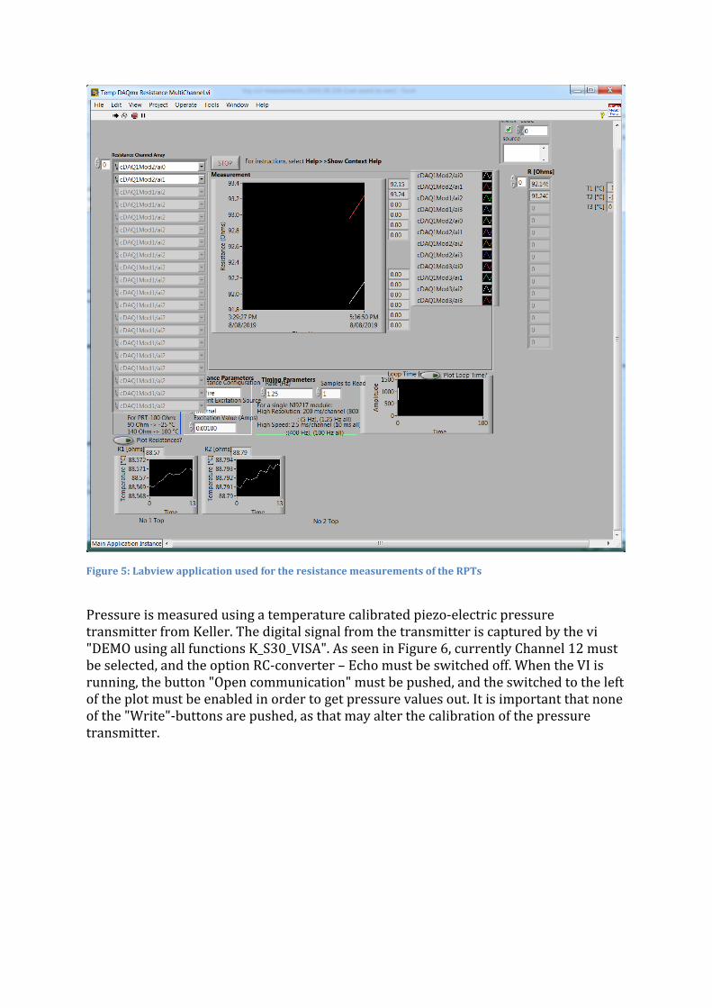
Figure 5: Labview application used for the resistance measurements of the RPTs

Pressure is measured using a temperature calibrated piezo-electric pressure transmitter from Keller. The digital signal from the transmitter is captured by the vi "DEMO using all functions K_S30_VISA". As seen in Figure 6, currently Channel 12 must be selected, and the option RC-converter – Echo must be switched off. When the VI is running, the button "Open communication" must be pushed, and the switched to the left of the plot must be enabled in order to get pressure values out. It is important that none of the "Write"-buttons are pushed, as that may alter the calibration of the pressure transmitter.

Figure 6: VI for the measurement of pressure.

The pressure and temperature signals are logged by the VI VLE (UWA) Data Recorder Apr17.

In order to enhance heat transfer and obtain a more uniform temperature across the cell, a stirrer is operated, controlled by the application AML Stepper Motor with Globals, shown in Figure 7. Important settings here are channel, mixer speed, where recommended setting currently is 60 rpm, and "Timer to run", which should be set to a large number. In principle the controller should shut down the motor if the temperature increases too much, but in practice this does not seem to work very well. Hence, care should be taken if the motor makes unusual sounds or has frequent stops.

Figure 7: Labview application used to control the stirrer.

Balancing the bridge is performed with the Bridge Balancing vi shown in Figure 8, and the thermal conductivity measurement application "THW measurement with quartzdyne" shown in Figure 9. These are essentially the same applications as used in the previous measurements, but there are some differences in how the thermal conductivity measurement applications work in practice. Unlike previous experiments, pressure and temperature are not automatically fetched by the VI, but, as discussed above, recorded by an independent system. Hence, the of the TC measurement application is read from the Global Values.vi shown in Figure 10. In order to set the pressure and temperature, and hence get meaningful file names, this vi can be found by tracing the temperature and pressure values of the TC measurement vi, as indicated in Figure 9. Further, the composition must be set manually in the TC measurement vi itself. No other physical parameters that can be set in the vi will actually be used in the further analysis of the results, and they can therefore be ignored.

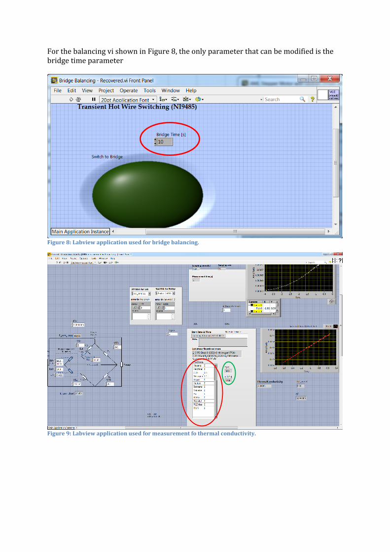
For the balancing vi shown in Figure 8, the only parameter that can be modified is the bridge time parameter

Figure 8: Labview application used for bridge balancing.

Figure 9: Labview application used for measurement fo thermal conductivity.

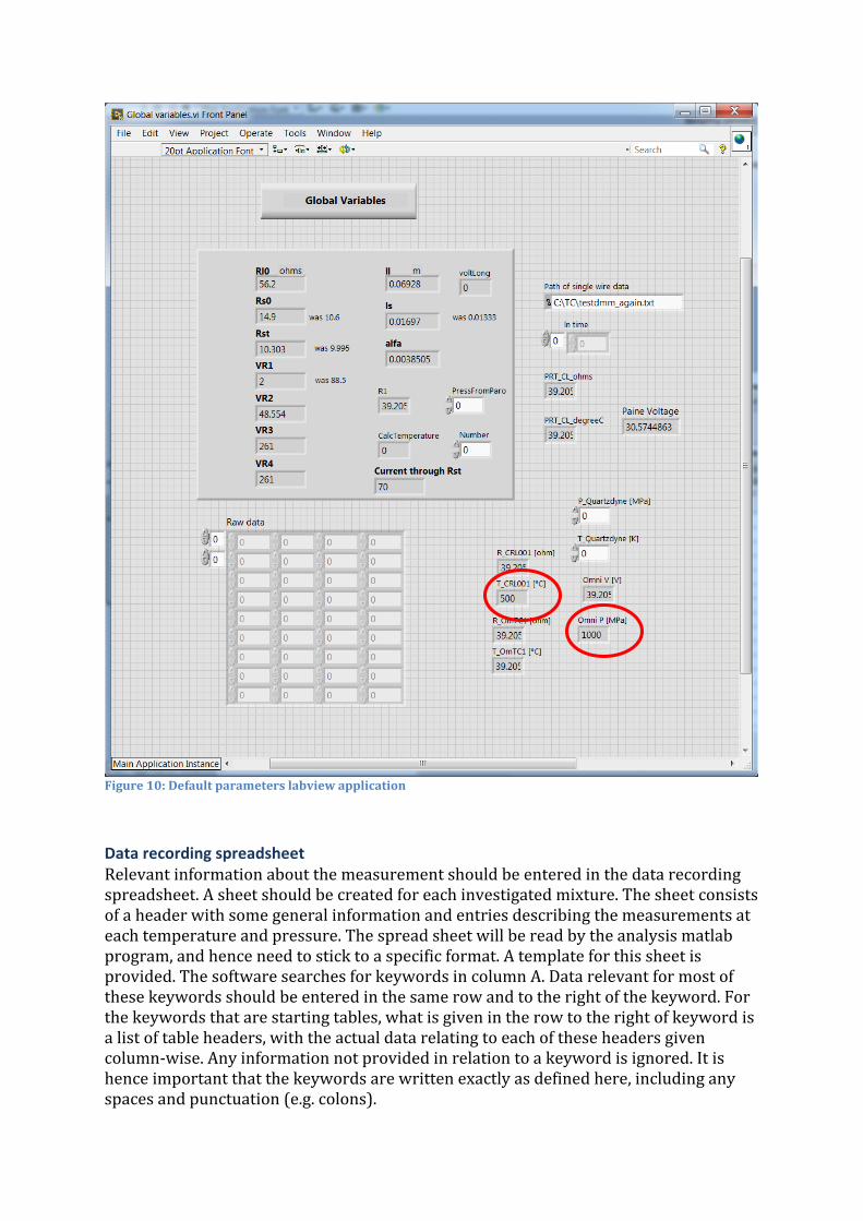
Figure 10: Default parameters labview application

Data recording spreadsheet Relevant information about the measurement should be entered in the data recording spreadsheet. A sheet should be created for each investigated mixture. The sheet consists of a header with some general information and entries describing the measurements at each temperature and pressure. The spread sheet will be read by the analysis matlab program, and hence need to stick to a specific format. A template for this sheet is provided. The software searches for keywords in column A. Data relevant for most of these keywords should be entered in the same row and to the right of the keyword. For the keywords that are starting tables, what is given in the row to the right of keyword is a list of table headers, with the actual data relating to each of these headers given column-wise. Any information not provided in relation to a keyword is ignored. It is hence important that the keywords are written exactly as defined here, including any spaces and punctuation (e.g. colons).

The header of a sheet is shown in Figure 11. The first row contains a description of the mixture, as well as the target value of 𝑉𝑉𝑠𝑠𝑠𝑠 during balancing. This value is used for each entry to calculate deviations between 𝑉𝑉𝑠𝑠𝑠𝑠 and this target value as well as proposing new values for 𝑅𝑅1 and 𝑅𝑅2. In addition, a value is given for the value 𝑉𝑉𝑠𝑠𝑠𝑠 during a measurement, assuming a supply voltage of 2.5 bar. Note that this a nominal value not corrected for bias for standard voltage present when no voltage has been applied. Neither of these values will be read by the analysis program, but the 𝑉𝑉𝑠𝑠𝑠𝑠 target value during balancing is used by the help tool for defining 𝑅𝑅1 in each entry. What is read from the header is the list of components, following and in the row of the keyword "Components:", and list of mole fractions, following the key word "Mole fractions:". The components must have the same names as the fluid files of REFPROP and TREND software, and the names must be provided in separate but consecutive columns following the keyword. The mole fraction for each component should be provided in the same column as its respective component name. The sum of the mole fractions should be one.

Figure 11: Header and first rows of an entry in a data recording spreadsheee

Each temperature / pressure measurement point is started by the "Included:" keyword which provides the date for when the measurement was started. Matlab is a bit picky when it comes to dates, so the selected "Locale" for the date field should be "English (United States)". In addition, with reference to the following column A keywords and corresponding information, the following data can be provided:

• "TFolder:" (required): This is the folder where the data from the TC measurement Labview application is stored. Only the lowest level of directory should be specified

• "Comment:" General information about the conditions during the experiment

• "R1:" (Required) The value of resistance 𝑅𝑅1. The value can be found by iteration as discussed above, and a new guess can be produced by the Excel spread sheet by entering the existing values of 𝑅𝑅1 and 𝑅𝑅2, measured values of 𝑉𝑉𝑠𝑠𝑠𝑠 (in mV), the standard measured when the balancing voltage is applied, and 𝑉𝑉𝑠𝑠𝑠𝑠,0 (mV), the average standard voltage when the bridge balancing application is run with 0 voltage supply voltage. Until beginning of August, what was provided here was the open-circuit standard voltage, but a closed circuit with zero applied voltage is probably value. Based on this information, adjusted values for 𝑅𝑅1 and 𝑅𝑅2 are suggested. Because the reading of 𝑉𝑉𝑠𝑠𝑠𝑠 has quite a bit of noise, it is sometimes better to enter a new value of 𝑅𝑅1 manually. The proposal for 𝑅𝑅2 will then be adjusted accordingly.

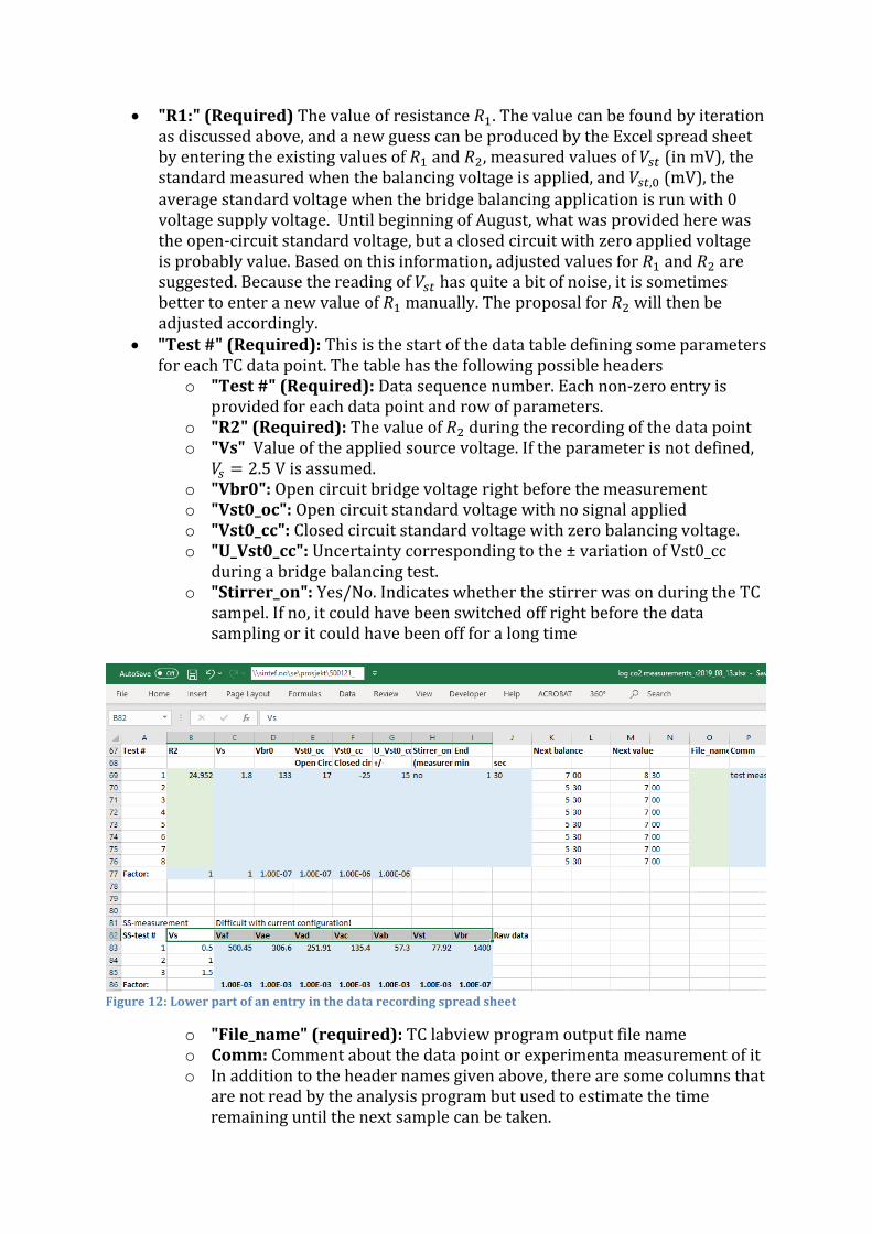
• "Test #" (Required): This is the start of the data table defining some parameters for each TC data point. The table has the following possible headers

o "Test #" (Required): Data sequence number. Each non-zero entry is provided for each data point and row of parameters.

o "R2" (Required): The value of 𝑅𝑅2 during the recording of the data point o "Vs" Value of the applied source voltage. If the parameter is not defined,

𝑉𝑉𝑠𝑠 = 2.5 V is assumed. o "Vbr0": Open circuit bridge voltage right before the measurement o "Vst0_oc": Open circuit standard voltage with no signal applied o "Vst0_cc": Closed circuit standard voltage with zero balancing voltage. o "U_Vst0_cc": Uncertainty corresponding to the ± variation of Vst0_cc

during a bridge balancing test. o "Stirrer_on": Yes/No. Indicates whether the stirrer was on during the TC

sampel. If no, it could have been switched off right before the data sampling or it could have been off for a long time

Figure 12: Lower part of an entry in the data recording spread sheet

o "File_name" (required): TC labview program output file name o Comm: Comment about the data point or experimenta measurement of it o In addition to the header names given above, there are some columns that

are not read by the analysis program but used to estimate the time remaining until the next sample can be taken.

• "Factor:" (required). This keyword signals the end of a table with data, either . In addition, scaling factors can be specified for each numerical parameter defined in the table.

• "SS-test #: Indicates the start of a table with steady state measurements, i. e. with the bridge engaged for a longer time. The table could have the following entries:

o "SS-test #" (Required if SS-test is reported): Data sequence number. Each non-zero entry is provided for each data point and row of parameters.

o "Vs" (Required if SS-test is reported): Supplied voltage 𝑉𝑉𝑠𝑠 during the SS-test.

o "Vax": Physical voltage between node A and node X, where X is any of the nodes (except A) indicated in Figure 2 (bridge circuit diagram) and (image of electrical wiring with indication of nodes).

o "Vst": Standard voltage 𝑉𝑉𝑠𝑠𝑠𝑠 when the supplied voltage is engaged o "Vbr": Bridge voltage 𝑉𝑉𝑏𝑏𝑏𝑏 when the supplied voltage is engaged

Data output files This is an overview of where data output files are saved currently, and their names. It would probably be wise to save all the output files in the folder ahead instead of the current locations:

• Output from temperature / pressure logging: The output files from logger of pressure / temperature program is saved in the directory C:\Labview data. The naming convention is that the first part of the file name should provide the start of the log in the format YYYY-MM-DD. E.g., for logging starting August 15th, 2019, the filename should start with "2019-08-15". The remainder of the filename can be used to describe what is logged, but is not interpreted by the matlab analysis program.

• TC measurement output: The output files from the TC measurement labview application is stored in the directory C:\TC\Data\<name describing the component>\<temperature in K in the format TTTK>. Filenames are generated automatically by the software, hence it is important to specify the temperature and pressure in that application, as discussed above.

• Excel data recording sheet: Can be placed in a location convenient for the user.