transient heat conduction in a circular cylinder - itll · pdf filetransient heat conduction...

APPM 4350/5350 Projects Updated December 18, 2014

Transient Heat Conduction in aCircular Cylinder

The purely radial 2-D heat equation will be solved in cylindrical coordinates using variation ofparameters. Assuming radial symmetry the solution is represented by a series of Bessel Functions.The solution is then compared with experimental results. The experimental apparatus is a circularcylinder heated from the inside with electricity and cooled on the outside with cold water.

I. Background

The heat equation is given by∂u

∂t− α52 u = 0, (1)

where u is the heat, α is the thermal diffusivity and 52u represents 5 · 5u, the divergence of thegradient of u. The heat equation is used to describe the diffusion of heat in a given region over time.In one dimension the solution is represented in terms of sines and cosines by a Fourier series.

On a cylinder the heat equation becomes slightly more cumbersome when written in terms ofu(r, θ). However, the experimental apparatus for this project has no way to measure the θ-dependenttemperature distributions, so we focus on the purely radial 2-D heat equation. The problem ofpurely radial heat conduction is also a one-dimensional problem but the solution is represented interms of Bessel functions as opposed to Fourier series. The purely radial 2-D heat heat equationwith forcing is given by

∂v

∂t= α

[1

r

∂

∂r

(r∂v

∂r

)]+ F (r, t), Ri < r < R0, t > 0

v(Ri, t) = g(t)

v(R0, t) = h(t)

v(r, 0) = V (r) Ri < r < R0,

(2)

where v is the measured heat, α is the thermal diffusivity, Ri is the radius of the inside measurement,R0 is the radius of the outside measurement, g(t) and h(t) represent the heating and cooling asfunctions of time respectively (both have units ◦c), and V (r)(◦c) represents the initial temperatureas a function of radius. In this experiment F (r, t) = 0 and can be ignored. (2) features somethingthat has not been accounted for in this class: time-dependent boundary conditions. The techniqueof variation of parameters is used to solve (2) with time-dependent boundary conditions. For theunfamiliar reader, the method of variation of parameters is explained in §IV.

II. Materials/Equipment

• 1 Control Box

• 1 Power Regulator

• 1 Selector Box

• 1 Radial conduction apparatus

• 1 Water chiller

For the analysis it may be important to know the dimensions of the cylinder.Cylinder Dimensions:

1


• Outer Radius: 150mm

• Height: 35mm.

The first temperature probe is located at the center of the cylinder and the other probes are locatedat 10mm intervals. This means that the 6th probe is located at r = 50mm. The probe at the centerrecords g(t) while the probe on the outside records h(t) in equation (2). All probes are laid in thesame piece of brass. The cylinder is heated from the inside by an electric heater in the middle andcooled from the outside by the cool water running along the outside of the cylinder.

III. Procedure

Setting Up the Apparatus

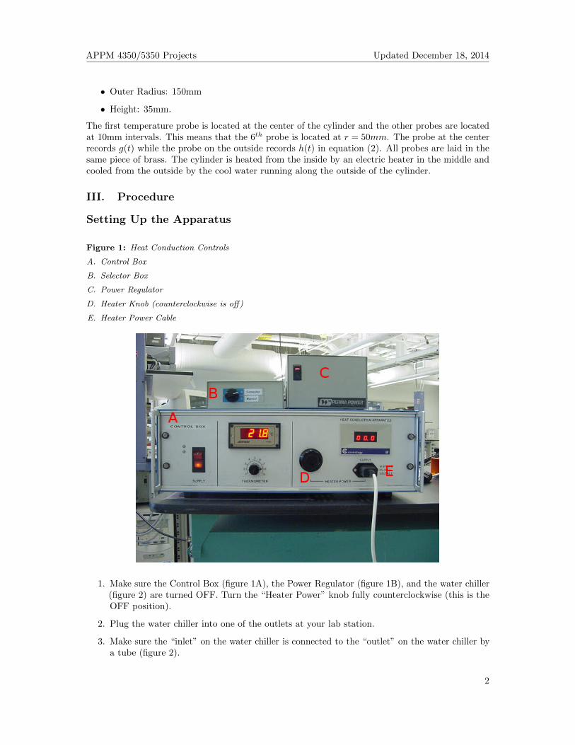
Figure 1: Heat Conduction Controls

A. Control Box

B. Selector Box

C. Power Regulator

D. Heater Knob (counterclockwise is off)

E. Heater Power Cable

APPM 4350/5350 Projects Updated November 9, 2013

• Outer Radius: 150mm

• Height: 35mm.

The first temperature probe is located at the center of the cylinder and the other probes are locatedat 10mm intervals. This means that the 6th probe is located at r = 50mm. The probe at the centerrecords g(t) while the probe on the outside records h(t) in equation (2). All probes are laid in thesame piece of brass. The cylinder is heated from the inside by an electric heater in the middle andcooled from the outside by the cool water running along the outside of the cylinder.

III. Procedure

Setting Up the Apparatus

Figure 1: Heat Conduction Controls

A. Control Box

B. Selector Box

C. Power Regulator

D. Heater Knob (counterclockwise is o↵)

E. Heater Power Cable

1. Make sure the Control Box (figure 1A), the Power Regulator (figure 1B), and the water chiller(figure 2) are turned OFF. Turn the “Heater Power” knob fully counterclockwise (this is theOFF position).

2. Plug the water chiller into one of the outlets at your lab station.

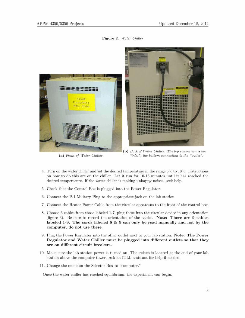
3. Make sure the “inlet” on the water chiller is connected to the “outlet” on the water chiller bya tube (figure 2).

2

1. Make sure the Control Box (figure 1A), the Power Regulator (figure 1B), and the water chiller(figure 2) are turned OFF. Turn the “Heater Power” knob fully counterclockwise (this is theOFF position).

2. Plug the water chiller into one of the outlets at your lab station.

3. Make sure the “inlet” on the water chiller is connected to the “outlet” on the water chiller bya tube (figure 2).

2


Figure 2: Water Chiller

(a) Front of Water Chiller(b) Back of Water Chiller. The top connection is the

“inlet”, the bottom connection is the “outlet”.

4. Turn on the water chiller and set the desired temperature in the range 5◦c to 10◦c. Instructionson how to do this are on the chiller. Let it run for 10-15 minutes until it has reached thedesired temperature. If the water chiller is making unhappy noises, seek help.

5. Check that the Control Box is plugged into the Power Regulator.

6. Connect the P-1 Military Plug to the appropriate jack on the lab station.

7. Connect the Heater Power Cable from the circular apparatus to the front of the control box.

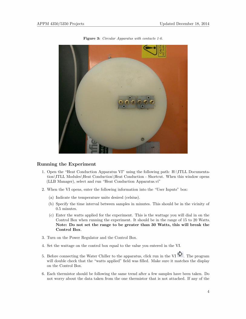
8. Choose 6 cables from those labeled 1-7, plug these into the circular device in any orientation(figure 3). Be sure to record the orientation of the cables. Note: There are 9 cableslabeled 1-9. The cords labeled 8 & 9 can only be read manually and not by thecomputer, do not use these.

9. Plug the Power Regulator into the other outlet next to your lab station. Note: The PowerRegulator and Water Chiller must be plugged into different outlets so that theyare on different circuit breakers.

10. Make sure the lab station power is turned on. The switch is located at the end of your labstation above the computer tower. Ask an ITLL assistant for help if needed.

11. Change the mode on the Selector Box to “computer.”

Once the water chiller has reached equilibrium, the experiment can begin.

3


Figure 3: Circular Apparatus with contacts 1-6.

Running the Experiment

1. Open the “Heat Conduction Apparatus VI” using the following path: H:\ITLL Documenta-tion\ITLL Modules\Heat Conduction\Heat Conduction - Shortcut. When this window opens(LLB Manager), select and run “Heat Conduction Apparatus.vi”

2. When the VI opens, enter the following information into the “User Inputs” box:

(a) Indicate the temperature units desired (celsius).

(b) Specify the time interval between samples in minutes. This should be in the vicinity of0.5 minutes.

(c) Enter the watts applied for the experiment. This is the wattage you will dial in on theControl Box when running the experiment. It should be in the range of 15 to 20 Watts.Note: Do not set the range to be greater than 30 Watts, this will break theControl Box.

3. Turn on the Power Regulator and the Control Box.

4. Set the wattage on the control box equal to the value you entered in the VI.

5. Before connecting the Water Chiller to the apparatus, click run in the VI . The programwill double check that the “watts applied” field was filled. Make sure it matches the displayon the Control Box.

6. Each thermistor should be following the same trend after a few samples have been taken. Donot worry about the data taken from the one thermistor that is not attached. If any of the

4


thermistors seem not to be reporting the same trend in the data as the other 6, try wiggling itin the probe to change the contact. If the thermistor is still not reporting the same trend asthe other 6 try switching it out for the extra thermistor (the cable not in use).

7. Once you are confident that the thermistors are providing reasonable data turn off the WaterChiller.

8. Disconnect the tube on the water chiller and attach the cooler tubes to the tubes coming fromthe conduction apparatus.

9. Turn the water chiller back on. Note when this occurs on your data, this is t = 0 for yourexperiment.

10. Continue taking measurements until the experiment reaches steady state. This should takeabout 10-20 minutes. When the experiment reaches steady state hit “STOP” and save thedata with a .xls extension.

11. Repeat this procedure multiple times if desired (once should suffice, but if you want someredundancy, do it again). Before each new trial, turn off the water chiller and let the conductionapparatus reach the same temperature (or higher) than you were seeing before turning thewater on in the previous trial.

12. When finished with the experiment, turn everything off and disconnect all cables. Make sureto clean up any excess water that fell on the floor. Return the module to the checkout.

IV. Analysis

Variation of Parameters

During the semester, we learned how to solve the heat equation with fixed temperatures (or fixedheat fluxes) at the boundaries. The purpose of this section is to generalize that procedure, to handletime-dependent forcing in the equation itself, or at the boundaries, or both.

A. Variation of Parameters ExplanationVariation of Parameters is a method to solve linear, ordinary differential equations (ODEs) withknown forcing. The heat equation is a linear partial differential equation that is first-order intime, and Variation of Parameters is especially simple for first-order (in time) ODEs. For higherorder ODEs, there is one additional logical step in the method, which is discussed in many bookson ODEs.

Consider a first-order, linear ODE with a constant coefficient, α, and a known forcing function,f(t):

dy

dt+ αy = f(t), y(0) = A (3)

(i) Solve the homogeneous ODE (i.e., with f(t) = 0):

yh(t) = ce−αt (4)

where c is the arbitrary constant of integration, or “parameter” in the solution.

5


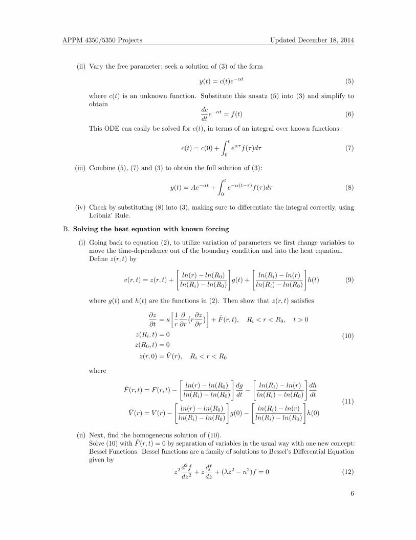
(ii) Vary the free parameter: seek a solution of (3) of the form

y(t) = c(t)e−αt (5)

where c(t) is an unknown function. Substitute this ansatz (5) into (3) and simplify toobtain

dc

dte−αt = f(t) (6)

This ODE can easily be solved for c(t), in terms of an integral over known functions:

c(t) = c(0) +

∫ t

0

eατf(τ)dτ (7)

(iii) Combine (5), (7) and (3) to obtain the full solution of (3):

y(t) = Ae−αt +

∫ t

0

e−α(t−τ)f(τ)dτ (8)

(iv) Check by substituting (8) into (3), making sure to differentiate the integral correctly, usingLeibniz’ Rule.

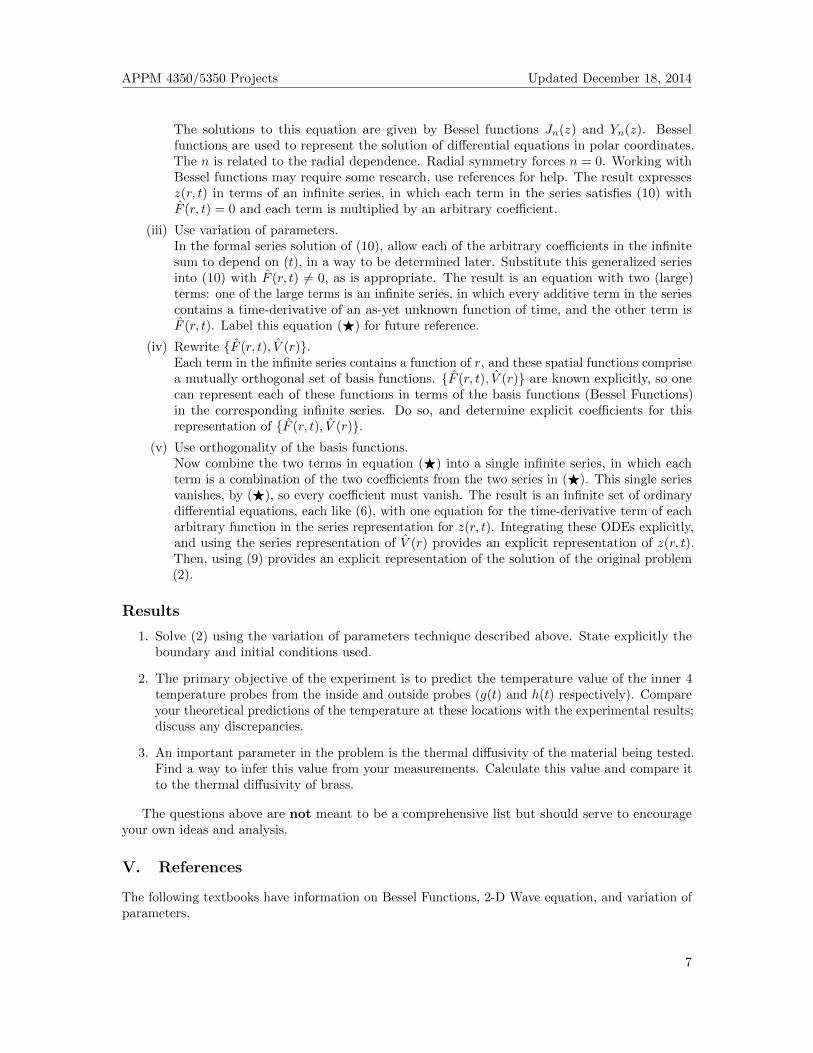
B. Solving the heat equation with known forcing

(i) Going back to equation (2), to utilize variation of parameters we first change variables tomove the time-dependence out of the boundary condition and into the heat equation.Define z(r, t) by

v(r, t) = z(r, t) +

[ln(r)− ln(R0)

ln(Ri)− ln(R0)

]g(t) +

[ln(Ri)− ln(r)

ln(Ri)− ln(R0)

]h(t) (9)

where g(t) and h(t) are the functions in (2). Then show that z(r, t) satisfies

∂z

∂t= κ

[1

r

∂

∂r

(r∂z

∂r

)]+ F̂ (r, t), Ri < r < R0, t > 0

z(Ri, t) = 0

z(R0, t) = 0

z(r, 0) = V̂ (r), Ri < r < R0

(10)

where

F̂ (r, t) = F (r, t)−[ln(r)− ln(R0)

ln(Ri)− ln(R0)

]dg

dt−[ln(Ri)− ln(r)

ln(Ri)− ln(R0)

]dh

dt

V̂ (r) = V (r)−[ln(r)− ln(R0)

ln(Ri)− ln(R0)

]g(0)−

[ln(Ri)− ln(r)

ln(Ri)− ln(R0)

]h(0)

(11)

(ii) Next, find the homogeneous solution of (10).Solve (10) with F̂ (r, t) = 0 by separation of variables in the usual way with one new concept:Bessel Functions. Bessel functions are a family of solutions to Bessel’s Differential Equationgiven by

z2d2f

dz2+ z

df

dz+ (λz2 − n2)f = 0 (12)

6


The solutions to this equation are given by Bessel functions Jn(z) and Yn(z). Besselfunctions are used to represent the solution of differential equations in polar coordinates.The n is related to the radial dependence. Radial symmetry forces n = 0. Working withBessel functions may require some research, use references for help. The result expressesz(r, t) in terms of an infinite series, in which each term in the series satisfies (10) withF̂ (r, t) = 0 and each term is multiplied by an arbitrary coefficient.

(iii) Use variation of parameters.In the formal series solution of (10), allow each of the arbitrary coefficients in the infinitesum to depend on (t), in a way to be determined later. Substitute this generalized seriesinto (10) with F̂ (r, t) 6= 0, as is appropriate. The result is an equation with two (large)terms: one of the large terms is an infinite series, in which every additive term in the seriescontains a time-derivative of an as-yet unknown function of time, and the other term isF̂ (r, t). Label this equation (F) for future reference.

(iv) Rewrite {F̂ (r, t), V̂ (r)}.Each term in the infinite series contains a function of r, and these spatial functions comprisea mutually orthogonal set of basis functions. {F̂ (r, t), V̂ (r)} are known explicitly, so onecan represent each of these functions in terms of the basis functions (Bessel Functions)in the corresponding infinite series. Do so, and determine explicit coefficients for thisrepresentation of {F̂ (r, t), V̂ (r)}.

(v) Use orthogonality of the basis functions.Now combine the two terms in equation (F) into a single infinite series, in which eachterm is a combination of the two coefficients from the two series in (F). This single seriesvanishes, by (F), so every coefficient must vanish. The result is an infinite set of ordinarydifferential equations, each like (6), with one equation for the time-derivative term of eacharbitrary function in the series representation for z(r, t). Integrating these ODEs explicitly,and using the series representation of V̂ (r) provides an explicit representation of z(r, t).Then, using (9) provides an explicit representation of the solution of the original problem(2).

Results

1. Solve (2) using the variation of parameters technique described above. State explicitly theboundary and initial conditions used.

2. The primary objective of the experiment is to predict the temperature value of the inner 4temperature probes from the inside and outside probes (g(t) and h(t) respectively). Compareyour theoretical predictions of the temperature at these locations with the experimental results;discuss any discrepancies.

3. An important parameter in the problem is the thermal diffusivity of the material being tested.Find a way to infer this value from your measurements. Calculate this value and compare itto the thermal diffusivity of brass.

The questions above are not meant to be a comprehensive list but should serve to encourageyour own ideas and analysis.

V. References

The following textbooks have information on Bessel Functions, 2-D Wave equation, and variation ofparameters.

7


1. Asmar N. Partial Differential Equations with Fourier Series and Boundary Value Problems.2nd edition. Prentice Hall; 2004.

2. Haberman, R. Applied Partial Differential Equations with Fourier Series and Boundary ValueProblems. 4th edition. Pearson Prentice Hall; 2004.

3. Pinsky, M. Partial Differential Equations and Boundary-Value Problems with Applications.3rd edition. Waveland Press; 2003.

8

transient heat conduction in a circular cylinder - itll · pdf filetransient heat conduction...

Documents