Transformation Properties ofthe Lagrangian and Eulerian

Strain Tensors

ARL-TR-908 April 2002

Thomas B. Bahder

Approved for public release; distribution unlimited.

The findings in this report are not to be construed as anofficial Department of the Army position unless sodesignated by other authorized documents.

Citation of manufacturer’s or trade names does notconstitute an official endorsement or approval of the usethereof.

Destroy this report when it is no longer needed. Do notreturn it to the originator.

ARL-TR-908 April 2002

Army Research LaboratoryAdelphi, MD 20783-1197

Transformation Properties ofthe Lagrangian and EulerianStrain TensorsThomas B. Bahder Sensors and Electron Devices Directorate

Approved for public release; distribution unlimited.

Abstract

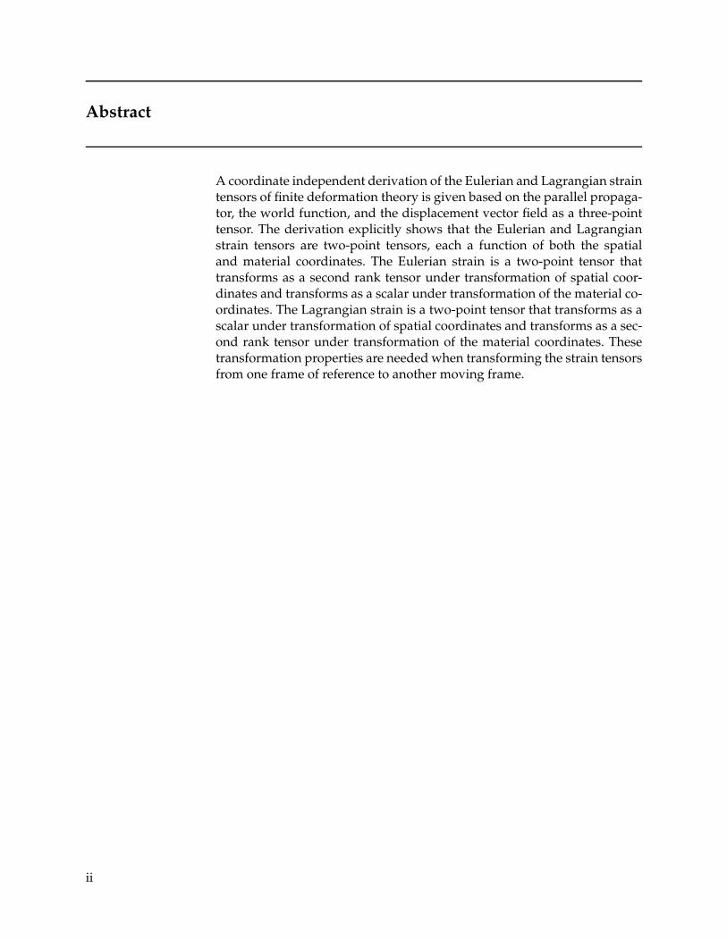
A coordinate independent derivation of the Eulerian and Lagrangian straintensors of finite deformation theory is given based on the parallel propaga-tor, the world function, and the displacement vector field as a three-pointtensor. The derivation explicitly shows that the Eulerian and Lagrangianstrain tensors are two-point tensors, each a function of both the spatialand material coordinates. The Eulerian strain is a two-point tensor thattransforms as a second rank tensor under transformation of spatial coor-dinates and transforms as a scalar under transformation of the material co-ordinates. The Lagrangian strain is a two-point tensor that transforms as ascalar under transformation of spatial coordinates and transforms as a sec-ond rank tensor under transformation of the material coordinates. Thesetransformation properties are needed when transforming the strain tensorsfrom one frame of reference to another moving frame.

ii

Contents

1 Background 1

2 Introduction 2

3 Geometric Background 4

3.1 The World Function . . . . . . . . . . . . . . . . . . . . . . . . 4

3.2 Parallel Propagator . . . . . . . . . . . . . . . . . . . . . . . . 8

3.3 Position Vector . . . . . . . . . . . . . . . . . . . . . . . . . . . 10

3.4 Displacement Vector . . . . . . . . . . . . . . . . . . . . . . . 11

4 Strain Tensors 15

4.1 Strain Tensor Derivation in Curvilinear Coordinates . . . . . 16

5 Strain Tensors in Terms of the Displacement Field 19

6 Summary 21

Acknowledgments 22

References 23

Distribution 27

Report Documentation Page 29

Figures

1 A geodesic path is shown in three dimensions with tangent unitvector at the ends . . . . . . . . . . . . . . . . . . . . . . . . . . . 7

2 The initial and final position vectors, R(P ) and r(Q), respec-tively, are shown as well as their respective parallel translatedvectors, R(P ) and r(Q). Also, shown by a solid curve is the ac-tual displacement path of a representative particle of the medium,labeled by zk = zk(Zm, t) . . . . . . . . . . . . . . . . . . . . . . . 12

3 The position P1 and P2 of two particles is shown in the referenceconfiguration at t = to, and the positions Q1 and Q2 of the sametwo particles is shown at later time t > to . . . . . . . . . . . . . 15

iii

1. Background

The U.S. Army is developing an electromagnetic gun (EMG) for battlefieldapplications. During the past few years, on a recurring basis, Dr. John Lyons(ARL Director) and Dr. W. C. McCorkle (Director of U. S. Army Aviationand Missile Command) have requested that I look at some of the physicsof the EMG. In the most recent request, I was asked to look at stresses ina rotating cylinder. For an elastic cylinder, this is a classic problem that issolved in many texts on linear elasticity [1–6]. However, when these deriva-tions are examined closely, one finds certain shortcomings [7]. Therefore, Ispent some time looking at the problem of stresses in elastic rotating cylin-ders, which resulted in a manuscript [7]. In the course of this work [7],I had to clearly understand the transformation properties of the Largan-gian and Eulerian strain tensors of finite deformation theory. I was quitedissatisfied with the standard derivations of the Largangian and Eulerianstrain tensors because these derivations take either of two (both unpalat-able) approaches. The first approach uses shifter tensors, which are oftendefined as inner products between two basis vectors at two different spatiallocations [8,9]. In this approach, basis vectors are not parallel transportedto the same spatial location before the inner product is carried out. Thisis unpalatable, even in Euclidean space, unless one is using Cartesian co-ordinates. The second approach uses convected (moving) coordinates, andvectors and tensors are associated with a given coordinate in the convected(moving) coordinate system, rather than being associated with a point inthe underlying space.

In the derivation that I present below, I avoid both of the unpalatable fea-tures mentioned above. I provide a coordinate independent derivation ofthe Lagrangian and Eulerian strain tensors based on standard concepts indifferential geometry: the parallel propagator, the world function, and thedisplacement vector field as a three-point tensor.

The derivation that I present below is also useful for gaining a basic under-standing of the role of the unstrained state, or reference configuration, inthe definition of the strain tensors. Having a firm conceptual grasp of therole of the unstrained state in the definition of the strain tensors is imper-ative for understanding the behavior of pre-stressed materials under finitedeformations in high-stress applications, such as, for example, in the elec-tromagnetic rail gun [10].

1

2. Introduction

The theory of stresses in rotating cylinders and disks is of great importancein practical applications such as rotating machinery, turbines and genera-tors, and wherever large rotational speeds are used. In a previous work [7],I gave a detailed treatment of stresses in a rotating elastic cylinder. This is aclassic problem that is treated in many texts on linear Elasticity theory [2–6].These treatments linearize the strain tensor in the gradient of the displace-ment field, assuming that these (dimensionless) gradients are small. Forlarge angles of rotation, the quadratic terms (in displacement gradient inthe definition of strain) are as large as the linear terms, and consequently,these quadratic terms cannot be dropped [7]. In Ref [7], I provide an al-ternative derivation of stresses in an elastic cylinder that relies on trans-forming the problem from an inertial frame (where Newton’s second lawis valid) to the co-rotating frame of the cylinder, where the displacementgradients are small. During the course of that solution, I had to transformthe Lagrangian and Eulerian strain tensors of finite elasticity to the (non-inertial) co-rotating frame of reference of the cylinder, which is a moving,accelerated frame. This work required the detailed understanding of thetransformation properties of the Lagrangian and Eulerian strain tensors.

The standard derivation of these strain tensors is done with the help ofshifter tensors [8,9]. Shifter tensors are often defined in terms of inner prod-ucts of basis vectors that are located at two different spatial points [8,9].For me, inner products between vectors at two different points is an un-palatable operation, even in Euclidean space. In order to compute the innerproduct between two vectors, the vectors must first be parallel transportedto the same spatial point (unless we are using Cartesian coordinates, inwhich case the derivation becomes coordinate specific).

In other treatments, where shifter tensors are not employed in the deriva-tion of strain tensors, convected (moving) coordinates are used, see for ex-ample [11–14]. When using convected (moving) coordinates, the coordi-nates of the initial undeformed point and the deformed point are the same,but the basis vectors change during deformation. In derivations of straintensors using convected coordinates, vectors and tensors are associatedwith a given point in the convected (moving) coordinate system, ratherthan being associated with a point in the underlying (inertial) space. Ten-sors are absolute geometric objects, and they should properly be associatedwith a point in the underlying space, and not a given coordinate, e.g., inmoving coordinates.

In this work, I avoid the unpalatable features of the strain tensor derivationmentioned in the above two paragraphs. I derive the strain tensors usingthe concept of absolute tensors, where a tensor is associated with a point

2

in the space, rather than the coordinates in a given (moving) coordinatesystem. I provide a coordinate independent derivation of the Lagrangianand Eulerian strain tensors, where I keep track of the positions of the basisvectors. The derivation necessarily uses two-point (and three-point) ten-sors [8,9,15,16]. The derivation is based on standard concepts in differen-tial geometry: the parallel propagator (a two-point tensor), the world func-tion (a two-point scalar), and the displacement vector field (a three-pointtensor). This derivation makes clear the transformation properties of thestrain tensors under coordinate transformations from one frame of refer-ence to a second frame that is moving and accelerated (with respect to thefirst frame).

The derivation below of the Eulerian and Lagrangian strain tensors makesthe transformation properties (e.g., to a moving frame) clear. Furthermore,this derivation makes the role of the reference (unstrained) configurationmore clear in the definition of the strain tensors. Clarifying this role is im-portant for applying finite deformation theory to pre-stressed materials,which are capable of withstanding higher-stress applications, such as in ro-tating machinery [7,10]. Finally, the derivation presented here allows thegeneralization of the definition of strain tensors to the realm where generalrelativity applies [17,18].

3

3. Geometric Background

In Euclidean space, a vector can be trivially parallel propagated in the sensethat after a round trip the vector still points in the same direction. In Rie-mannian space, the parallel displaced vector is not equal to itself after theround trip parallel displacement. In this sense, in Euclidean space we neednot distinguish the position of a vector because “it always points in thesame direction under parallel displacement,” even though its componentsmay be different from point to point because the basis vectors, onto whichwe project the vector, point in a different direction from point to point.So, in Euclidean space the parallel displaced (physical) vector (a geomet-ric object) is thought to point in the same physical direction. In Riemannianspace, however, the situation is quite different. In Riemannian space, a vec-tor that is parallel displaced will in general point in a different direction.The physical test is to parallel displace the vector along a curve that re-turns to the starting point. If there is non-zero curvature, as measured bythe Riemann curvature tensor, then upon returning to its starting point thevector components will be different than the initial vector components atthe starting point. So, in Reimannian space, it is imperative to specify theposition of a vector. In Euclidean space, appropriate to material deforma-tions, I also keep track of the position of a vector. This additional care inEuclidean space, together with the transformation properties of the worldfunction, leads to a clearer understanding of the transformation propertiesof the Lagrangean and Eulerian strain tensors, under transformations fromone system of coordinates to another that is in relative motion (a movingframe).

This section briefly reviews the fundamental geometric quantities that nat-urally arise in discussion of deformation, but which are not usually dis-cussed in this context. These quantities are the world function (or funda-mental two-point scalar of the the space), the parallel propagator, and theposition vector. This section will also serve to define my notation. Each ofthe quantities mentioned are examples of a class of geometric object knownas two-point tensors, which occur naturally in the discussion of deforma-tions. I have found useful discussions of general tensor calculus in Syngeand Schild [19] and Synge [16], and discussions oriented toward deforma-tion theory in the appendix by Ericksen in Treusdell and Toupin [15], and inNarasimhan [9], Eringen [8], and Eringen [20]. In particular, discussion oftwo-point tensors can be found in Synge [16], Ericksen [15], Narasimhan [9]and Eringen [8].

3.1 The World Function

The world function was initially introduced into tensor calculus byRuse [21,22], Synge [23], Yano and Muto [24], and Schouten [25]. It was

4

further developed and extensively used by Synge in applications to prob-lems dealing with measurement theory in general relativity [16]. An ap-plication of the world function to problems of navigation and time transfercan be found in Ref. [26]. Compared to the enormous attention given to ten-sors, the world function has been used very little by physicists. Yet, whengeometry plays a central role, such as in deformation theory, the worldfunction is helpful to clarify and unify the underlying geometric concepts.The world function is simply one-half the square of the distance betweentwo points in the space. In applications to relativity and four-dimensionalspace-time, the space-time is often taken as a general (curved) pseudo-Riemannian space [16]. In applications to deformation of materials, we areconcerned with a Euclidean three-dimensional space. However, for under-standing the transformation properties of displacement vectors and straintensors, it is helpful to use the concept of world function in a Euclideanthree-dimensional space described by curvilinear coordinates xi, i = 1, 2, 3,with a metric gij , which in general is a function of position.

Consider two points in a general Riemannian space, P1 and P2, connectedby a unique geodesic path (a straight line in Euclidean space) Γ, given byxi(u), i = 1, 2, 3, where u1 ≤ u ≤ u2, and xi(u) are curvilinear coordinatesof the path. The coordinates of point P1 = xi

1 and point P2 = xi2. In

general, a geodesic is defined by a class of special parameters u′, u · · ·, thatare related to one another by linear transformations u′ = au + b, wherea and b are constants. Here, u is a particular parameter from the class ofspecial parameters that define the geodesic Γ, and xi(u) satisfy the geodesicequations

d2xi

du2+ Γi

jk

dxj

du

dxk

du= 0 (1)

Using Cartesian coordinates zk (rather than general curvilinear coordinatesxk) in Euclidean space, the Christoffel symbol Γi

jk = 0, and the solution ofequation (1) is simply

zα(u) = zα1 +

u− u1

u2 − u1(zα

2 − zα1 ) (2)

where u1 ≤ u ≤ u2, i = 1, 2, 3 and the Cartesian coordinates of pointsP1 and P2 are zα

1 and zα2 , respectively. In a general Riemannin space, the

world function between point P1 and P2 is defined as the integral along Γin arbitrary curvilinear coordinates xi by

Ω(P1, P2) =12(u2 − u1)

∫ u2

u1

gijdxi

du

dxj

dudu (3)

The value of the world function has a simple geometric meaning: It is one-half the distance between points P1 and P2. Its value depends only on theeight coordinates of the points P1 and P2. The value of the world functionin equation (3) is independent of the particular special parameter u in thesense that under a transformation from one special parameter u to another,u′, given by u = au′ + b, with xi(u) = xi(u(u′)) and with a and b constant,

5

the world function definition in equation (3) has the same form (with ureplaced by u′).

The world function is the fundamental two-point invariant that character-izes the space. It is invariant under independent transformation of coordi-nates at P1 and at P2. For a given space, the world function between pointsP1 and P2 has the same value independent of the coordinates used, whichmakes it a useful coordinate independent quantity. In Euclidean space, us-ing Cartesian coordinates, the world function has the simple form

Ω(zi1, z

j2) =

12δij ∆zi ∆zj (4)

where δij is the Euclidean metric with only non-zero diagonal components(+1,+1,+1), and ∆zi = (zi

2 − zi1), i = 1, 2, 3, where zi

1 and zi2 are the Carte-

sian coordinates of points P1 and P2, respectively. (I use the convention thatall repeated indices are summed, unless otherwise stated.)

The world function has a number of interesting properties, see Synge [16].Calculations of the world function for spaces other than Euclidean spaces,namely four-dimensional space-time, can be found in Refs. [16,26–29]. Inwhat follows, I restrict myself to a three-dimensional space. By transform-ing to a new system of coordinates, say spherical coordinates,

x = r cos θ cosφ (5)

y = r cos θ sinφ (6)

z = r cos θ (7)

the world function in equation (4) can be expressed as a function of spheri-cal coordinates of point P1 = (r1, θ1, φ1), and P2 = (r2, θ2, φ2).

Consider a geodesic given by equation (1) in a general three-dimensionalRiemannian space. The covariant derivatives of the world function havetwo important properties:

∂ Ω(P1, P2)∂ xi

2

= (u2 − u1)

(gijdxj

du

)P2

= Lλi2 (8)

∂ Ω(P1, P2)∂ xi

1

= −(u2 − u1)

(gijdxj

du

)P1

= −Lλi1 (9)

where

L = [2 Ω(P1, P2)]1/2 =

∫ P2

P1

ds =∫ u2

u1

[gijdxi

du

dxj

du

]1/2

du (10)

is the length of the geodesic between P1 and P2, gij is the metric in coordi-nates xi, and λi1 and λi2 are components of the unit tangent vectors at endpoints P1 and P2 (assuming non-null geodesics [16]):

λi1 =

(gijdxj

ds

)P1

(11)

λi2 =

(gijdxj

ds

)P2

(12)

6

where the relation between parameter u and arc length s is given by equa-tion (10). In equations (8) and (9), the covariant partial derivatives withrespect to xi

1 and xi2 are done with respect to the coordinates of points P1

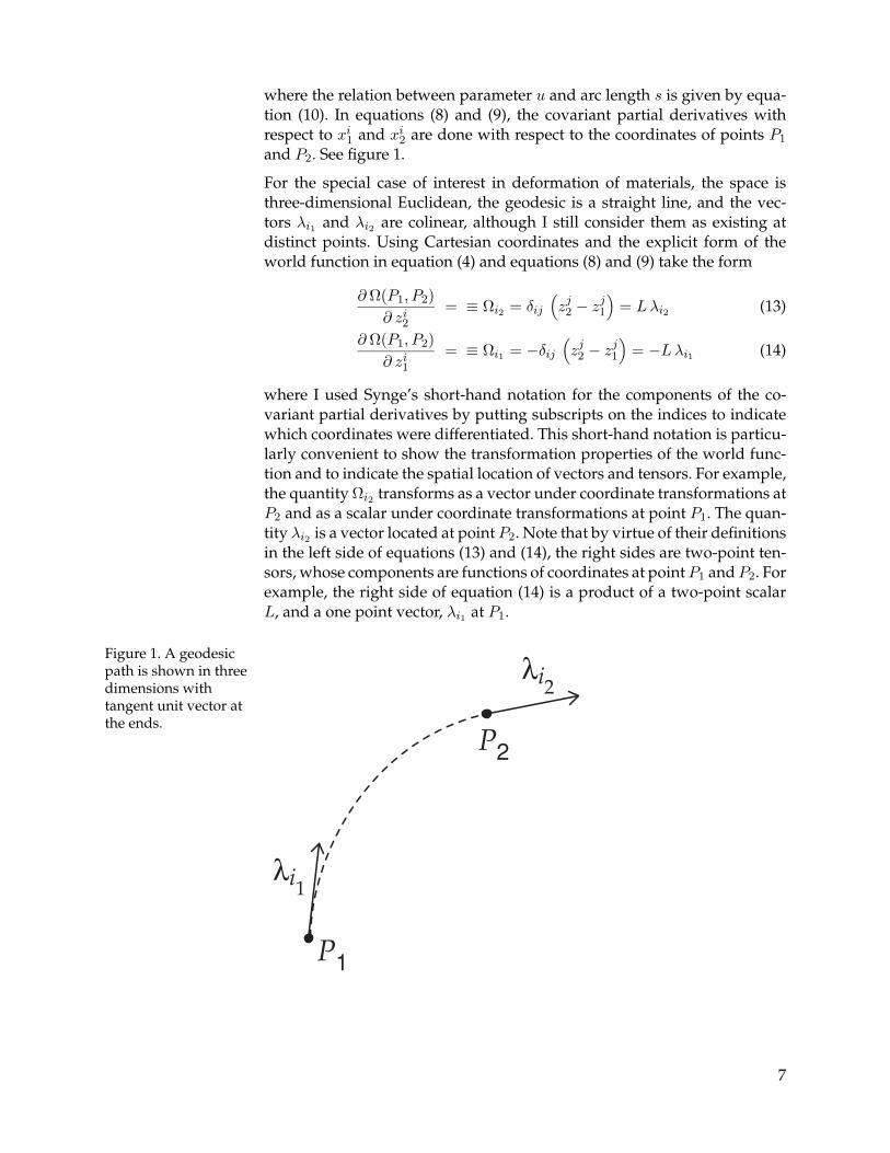
and P2. See figure 1.

For the special case of interest in deformation of materials, the space isthree-dimensional Euclidean, the geodesic is a straight line, and the vec-tors λi1 and λi2 are colinear, although I still consider them as existing atdistinct points. Using Cartesian coordinates and the explicit form of theworld function in equation (4) and equations (8) and (9) take the form

∂ Ω(P1, P2)∂ zi

2

= ≡ Ωi2 = δij(zj2 − z

j1

)= Lλi2 (13)

∂ Ω(P1, P2)∂ zi

1

= ≡ Ωi1 = −δij(zj2 − z

j1

)= −Lλi1 (14)

where I used Synge’s short-hand notation for the components of the co-variant partial derivatives by putting subscripts on the indices to indicatewhich coordinates were differentiated. This short-hand notation is particu-larly convenient to show the transformation properties of the world func-tion and to indicate the spatial location of vectors and tensors. For example,the quantity Ωi2 transforms as a vector under coordinate transformations atP2 and as a scalar under coordinate transformations at point P1. The quan-tity λi2 is a vector located at point P2. Note that by virtue of their definitionsin the left side of equations (13) and (14), the right sides are two-point ten-sors, whose components are functions of coordinates at pointP1 andP2. Forexample, the right side of equation (14) is a product of a two-point scalarL, and a one point vector, λi1 at P1.

Figure 1. A geodesicpath is shown in threedimensions withtangent unit vector atthe ends.

λi2

P1

P2

λi1

7

3.2 Parallel Propagator

Given a vector with components vi1 at point P1, the vector is said to beparallel propagated from P1 to P2 along a geodesic curve C specified byxi(u), u1 ≤ u ≤ u2, where P1 = xi(u1) and P2 = xi(u2), when itscovariant derivative is zero along this curve:

dvi

du+ Γi

jk vj dx

k

du= 0 (15)

Equation (15) is a mapping: Given the components of a vector, vi1 at pointP1, we obtain the components vi2 of the parallel transported vector at pointP2 by solving equation (15). It is convenient to define a two-point tensor,gi2

j1, called the parallel propagator [16], which gives the components of a

vector under parallel translation of the vector from point P1 to point P2.Given a vector with components vi1 at point P1, the propagator gi2

j1relates

the components of this vector at P1 to the components vi2 of this same vec-tor after parallel translation to point P2

vi2 = gi2i1vi1 (16)

In a general Riemannian space, the components of the vector at point P2

depend on the path of parallel translation from P1 to P2, in the sense thatthe path must be a geodesic by the definition of the parallel propagator.However, in Euclidean space these components are completely path inde-pendent; the components depend only on the end points P1 and P2.

A vector is considered as a geometric object, which means that it is inde-pendent of coordinate system. In a Riemannian space, under the operationof parallel propagation a vector changes in such a way that its magnitudestays the same but its absolute direction can change because of the curva-ture of the space [30]. The direction of the parallel propagated vector is, ofcourse, referred to the local basis vectors. That the vector direction changesunder parallel translation can be understood by taking a vector at point Pand parallel translating it over a curve that returns to point P . When com-pared at point P , the components of the initial vector and the round-trip-parallel-transported vector will (in general) be different. It is in this sensethat a vector changes its direction under parallel transport.

As mentioned above, the change in the vector that results under paralleltransport depends on the path of parallel propagation (a geodesic). Twovectors that are parallel propagated along the same path will maintain theangle between them along the path.

In a Euclidean space, a vector (the geometric object) is considered to beunchanged when parallel propagated. The only thing that happens is thatthe components of the vector on the local basis must change according towhat is required to keep the vector “pointing in the same direction.”

In Euclidean space, the parallel propagator in Cartesian coordinates istrivial—its components are just the components of a delta function. The

8

components of a vector at point P1 are related to the components of thesame vector parallel translated to point P2 by the propagator (whose com-ponents are given in a Cartesian coordinate basis):

δi2j1 =

+1 i = j

0 i = j(17)

Equation (17) agrees with our notion from elementary geometry that inCartesian coordinates the vector components are constant under parallelpropagation. However, using the parallel propagator in Cartesian coordi-nates, we can, for example, compute the propagator gi2

j1in curvilinear co-

ordinates xi = (r, θ, φ) given in equation (5)–(7), by the two-point tensortransformation rule

gi2j1

=∂ xi(P2)∂ zm

∂ zn(P1)∂ xj

δm2n1

(18)

The parallel propagator gi2j1

is a two-point tensor because it transforms asa vector under coordinate transformation at point P1 and under coordinatetransformation at point P2.

In Cartesian coordinates, when the points are made to coincide, P2 → P1,the propagator reduces to a Kronecker delta at point P1: δm2

n1→ δmn(P1).

In general curvilinear coordinates, when the points P1 and P2 coincide, theparallel propagator reduces to the mixed components of the metric tensorgi2

j1:

limP2→P1

gi2j1

→ gij(P1) (metric at P1) (19)

The mixed components of the metric tensor at P1, gij(P1) ≡ gik(P1) gkj(P1),

are a Kronecker delta—a unit tensor whose components are the same in allsystems of coordinates. Indices can be lowered on two-point tensors usingthe appropriate metric. For example, the index i of the propagator gi2

j1can

be lowered by using the metric tensor at point P2:

gk2j1 = gki(P2) gi2j1

(20)

When the points are made to coincide, P2 → P1, the covariant componentsof the propagator become the covariant components of the metric tensor atP1, gk2j1 → gkj(P1), where gkj(P1) is the metric at P1.

The covariant derivatives of the world function Ω(P1, P2) between pointsP1 and P2 are related to the parallel propagator by [16]

Ωi1j1 = gi1j1 (metric at P1) (21)

Ωi1j2 = Ωj2i1 = −gi1j2 = −gj2i1 (parallel propagator) (22)

Ωi2j2 = gi2j2 (metric at P2) (23)

Other useful properties of the parallel propagator are discussed by Synge [16].

9

3.3 Position Vector

The position vector occupies a central role in deformation theory. For thisreason, I discuss it in detail below. In elementary geometry, a point P canbe identified by its position vector r, which can be specified in Euclidean-space Cartesian coordinates as

r = zn in (24)

where zn are the Cartesian components of the vector r and also the Carte-sian coordinates of the point P . In terms of general coordinate basis vectorsen = ∂/∂xn associated with the curvilinear coordinates xn, the vector r isgiven by

r = znAmn(P ) em(P ) = ζm em(P ) (25)

The position vector is a geometric object at point P . Among all basis vec-tors, the Cartesian basis vectors in are unique in that they are usually notassociated with a particular spatial point. However, when we express theseCartesian basis vectors in terms of curvilinear basis vectors en, then wemust imagine that these basis vectors exist at a particular point P . Hence,the transformation between the Cartesian basis vector im and curvilinearcoordinate basis vectors em at point P associated with coordinates xi isgiven by

in(P ) = Amn(P ) em(P ) (26)

where the matrix Amn (P ) depends on the coordinates of point P :

Amn(P ) =

∂ xm

∂ zn(P ) (27)

In Cartesian coordinates, the components of the vector r are simply theCartesian coordinates zn of point P . The three numbers (z1, z2, z3) trans-form as the components of a vector under orthogonal coordinate transfor-mations. Note that in curvilinear coordinates, the components of the po-sition vector, ζm, are not the curvilinear coordinates of point P . Also, notethat the position vector r of point P has a magnitude equal to the Euclideanlength from the origin of coordinates, say point O, to point P . The positionvector of point P is a geometric object at point P , however, it also dependson the point O. This dependence on point O is coordinate independent.Therefore, the position vector of point P is a two-point tensor; it dependson point P and on point O. The transformation properties of the positionvector are that of a scalar when a change of coordinates is made at point Oand the transformation is that of a vector when coordinates at point P arechanged.

In a Riemannian (a generalization of Euclidean space) space, the compo-nents of the position vector ri(P ) at point P can be defined in terms of thecovariant derivative of the world function

riP =∂ Ω(O,P )∂ zi

P

≡ ΩiP (O,P ) = [2 Ω(O,P )]1/2 ri(P ) (28)

10

where riP is a unit vector at point P and [2 Ω(O,P )]1/2 is the length of thegeodesic from point O to point P . For Euclidean space, [2 Ω(O,P )]1/2 isthe length of the straight line OP . Equation (28) shows explicitly that theposition vector, riP , is a two-point tensor.

3.4 Displacement Vector

Consider an elastic body that undergoes a finite deformation in time. Thedeformation can be specified by a flow function or displacement mappingfunction

zk = zk(Zm, t) (29)

where the coordinates zk (here taken to be Cartesian) of a particle at pointQ at time t are given in terms of the particle’s coordinates Zk of point Pin some reference state (configuration) at time t = to, so that zk(Zm, to) =Zk. We assume the deformation mapping function has an inverse, which isquoted here for later reference

Zm = Zm(zk, t) (30)

We assume that both the coordinates zk and Zm refer to the same Cartesiancoordinate system. ∗

In deformation theory, the initial position of the particle in the medium atpoint P is specified by a vector

R(P ) = Zk ik(P ) (31)

and the final position is specified by a position vector

r(Q) = zk ik(Q) (32)

where the quantities ik(P ) and ik(Q) are the Cartesian basis vectors at pointP and point Q, respectively. Conventionally, the deformation of a mediumis described by specifying the displacement “vector field,” which is definedas a difference of these two position vectors. However, the basis vectorsik(P ) and ik(Q) are at different points in the space. Since vectors can be sub-tracted only if they are at the same point, we must parallel translate ik(P ) topoint Q, or, parallel translate ik(Q) to point P . Depending on which map-ping we choose, we arrive at the Eulerian or the Lagrangian displacementvector.

First, we parallel translate vector R(P ) to point Q, and then subtract thevectors at point Q (see fig. 2). This procedure defines the components ofthe Eulerian displacement vector at point Q:

u(Q) = r(Q) − R(Q) (33)

∗I use the notation zk and Zk for the Cartesian coordinates and also for the deformationmapping functions. There is no chance of confusing these two since the context makes itclear which one is used in a given instant.

11

Figure 2. The initial andfinal position vectors,R(P ) and r(Q),respectively, are shownas well as theirrespective paralleltranslated vectors, R(P )and r(Q). Also, shownby a solid curve is theactual displacementpath of a representativeparticle of the medium,labeled byzk = zk(Zm, t). Thedashed straight line isthe line (geodesic)connecting the initialand final particlepositions. The Euleriandisplacement vector isu = r(Q)−R(Q), whichis the difference of twoposition vectors at pointQ. The Lagrangeandisplacement vector,U = r(P ) − R(P ), is thedifference of twoposition vectors at pointP .

U(P) = r(P) – R(P)

u(Q) = r(Q) – R(Q)

O

Q

P

zk = zk(Zm,t)

r(Q)R(Q)

R(P)

r(P)

This Eulerian displacement vector in equation (33) is often called the dis-placement vector in the spatial representation [8,9,31]. Alternatively, we canparallel translate the vector r(Q) to point P , and then subtract the vectorsat point P . This procedure defines the Lagrangian displacement vector atpoint P :

U(P ) = r(P ) − R(P ) (34)

This Lagrangian displacement vector in equation (34) is often called thedisplacement vector in the material representation [8,9,31]. Equations (33)and (34) show that these two vectors are actually referred to basis vectors atdifferent points. In fact, the two vectors u(Q) and U(P ) are related by par-allel translation. In a Euclidean space, these vectors are the same geometricobjects but they are expressed in terms of basis vectors located at differentpositions P and Q (see below).

In order to further clarify the transformation properties of these two dis-placement vectors, we use the position vector as discussed in the previoussection. Consider the deformation mapping function in curvilinear coordi-nates, xk(Xm, t). This function specifies the coordinates xk (point Q) of aparticle at current time t in terms of the coordinates Xk (point P ) of theparticle in the reference configuration at time t = to, so that

xk(Xm, to) = Xk (35)

12

In addition, there exists a straight line (a geodesic) Γ connecting the pointsP and Q.

The covariant components of the position vector of point P , R(P ) =Rn en(P ), in curvilinear coordinates xi are given by (see equation (28))

RiP =∂ Ω(O,P )∂ xi

P

≡ ΩiP (O,P ) = [2 Ω(O,P )]1/2 RiP (36)

where RiP are the components of the unit vector at point P tangent to Γthat connects point P and Q. Similarly, the covariant components of vectorr(Q) = rn en(Q) in curvilinear coordinates xi are given by

riQ =∂ Ω(O,Q)∂ xi

Q

≡ ΩiQ(O,Q) = [2 Ω(O,Q)]1/2 riQ (37)

where riQ are the components of the unit vector at point Q tangent to Γ.From equations (36) and (37) it is clear that both RiP and riQ are two-pointtensor objects. The quantity RiP depends on point O and P and transformsas a vector under coordinate transformations at P and as a scalar undercoordinate transformations at point O. The quantity riQ transforms as avector under coordinate transformations at point Q and as a scalar undercoordinate transformations at point O.

The components of the Eulerian displacement vector in equation (33) (atpoint Q) are defined in terms of the components of RiP parallel translatedto point Q:

RiQ = giQjPRjP (38)

= giQjP

ΩjP (O,P ) (39)

where ΩjP (O,P ) = gjk(P ) ΩkP(O,P ), and gjk(P ) is the metric at point P in

coordinates xi. The contravariant components of the Eulerian displacementvector in equation (33) are given by

uiQ = ΩiQ(O,Q) − giQjP

ΩjP (O,P ) (40)

Similarly, the components of the Lagrangian displacement vector are givenby

U iP = giPjQ

ΩjQ(O,Q) − ΩiP (O,P ) (41)

The vectors whose components are U iP and uiQ are related by paralleltransport along the geodesic Γ connecting P and Q (not along the parti-cle displacement line given by equation (29)). Transporting U iP to point Q

U iQ = giQkPUkP (42)

= giQjP

[gjP

kQΩkQ(O,Q) − ΩjP (O,P )

](43)

= δik(Q)ΩkQ(O,Q) − giQjP

ΩjP (O,P ) (44)

= uiQ (45)

13

where in the transition from equation (43) to (44) I have used the identitysatisfied by the parallel propagator:

δik(Q) = giQjPgjP

kQ(46)

where δik(Q) is a unit tensor (delta function) at point Q. Equation (46) isthe statement that parallel propagation of a vector has an inverse, so theresult that U i(P ) and ui(Q) are related by parallel transport is true in bothEuclidean and Reimannian spaces.

14

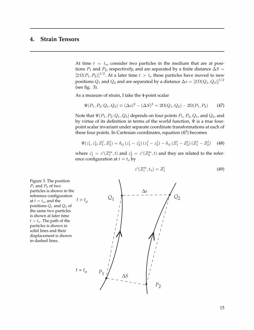
4. Strain Tensors

At time t = to, consider two particles in the medium that are at posi-tions P1 and P2, respectively, and are separated by a finite distance ∆S =[2 Ω(P1, P2)]

1/2. At a later time t > to these particles have moved to newpositions Q1 and Q2 and are separated by a distance ∆s = [2 Ω(Q1, Q2)]

1/2

(see fig. 3).

As a measure of strain, I take the 4-point scalar

Ψ(P1, P2;Q1, Q2) ≡ (∆s)2 − (∆S)2 = 2Ω(Q1, Q2) − 2Ω(P1, P2) (47)

Note that Ψ(P1, P2;Q1, Q2) depends on four points P1, P2, Q1, and Q2, andby virtue of its definition in terms of the world function, Ψ is a true four-point scalar invariant under separate coordinate transformations at each ofthese four points. In Cartesian coordinates, equation (47) becomes

Ψ(zi1, z

i2;Z

j1 , Z

j2) = δij (zi

1 − zi2) (zj

1 − zj2) − δij (Zi

1 − Zi2) (Zj

1 − Zj2) (48)

where zi1 = zi(Zm

1 , t) and zi2 = zi(Zm

2 , t) and they are related to the refer-ence configuration at t = to by

zi(Zm1 , to) = Zi

1 (49)

Figure 3. The positionP1 and P2 of twoparticles is shown in thereference configurationat t = to, and thepositions Q1 and Q2 ofthe same two particlesis shown at later timet > to. The path of theparticles is shown insolid lines and theirdisplacement is shownin dashed lines.

t > to

P2

∆SP1

t = to

Q2

∆sQ1

15

andzi(Zm

2 , to) = Zi2 (50)

and zi(Zm, t) is the deformation mapping function in Cartesian coordi-nates, given in equation (29). If the particle positions P1 and P2 are con-sidered as separated by an infinitesimal distance, then, by assuming conti-nuity in the medium and a finite time t − to, the points Q1 and Q2 are alsoinfinitesimally separated. However, because t− to is finite, the distance be-tween P1 andQ1 is finite (not infinitesimal). Expanding equation (50) aboutthe initial position of the first particle

zi2 = zi(Zk

1 , t) +∂ zi

∂ Zj(Zm

1 , t) (Zj2 − Zj

1) + · · · (51)

using zi1 = zi(Zk

1 , t), leads to the relation between spatial (Eulerian) coordi-nates zi and material (Lagrangian) coordinates Zk

∆zi =∂ zi

∂ Zj(Zm

1 , t) ∆Zj + · · · (52)

where ∆zi = zi2−zi

1 and ∆Zi = Zi2−Zi

1. Using equation (52) in equation (48)leads to the measure of strain in Cartesian coordinates

(∆s)2 − (∆S)2 =

(δij

∂ zi

∂ Zm

∂ zi

∂ Zn− δmn

)∆Zm ∆Zn + · · · (53)

= 2Emn ∆Zm ∆Zn + · · · (54)

where the quantity in parenthesis is the Lagrangean strain tensor,Emn. Thehigher order terms in ∆Zm are small because we can always choose thetwo initial points P1 and P2 arbitrarily close together. From equations (53)and (54), it is clear that the Lagrangean strain tensor is a two-point tensor,depending on initial point P (in the reference configuration at t = to) andpoint Q (at time t). Note that in equation (54) there is no restriction to shorttimes t− to, since we can always choose ∆Zn sufficiently small.

The Eullerian tensor can be obtained from equation (54) by using the factthat the flow function in equation (29) has an inverse. Using

∆Zn =∂Zn

∂zi(zi, t) ∆zi (55)

We get the measure of strain in terms of the Eulerian strain tensor emn:

(∆s)2 − (∆S)2 =

(δmn − δkl

∂ Zk

∂ zm

∂ Z l

∂ zn

)∆zm ∆zn + · · · (56)

= 2 emn ∆zm ∆zn + · · · (57)

4.1 Strain Tensor Derivation in Curvilinear Coordinates

I return to the definition of the measure of strain given in equation (47).In the reference configuration at t = to, consider two particles at points P1

16

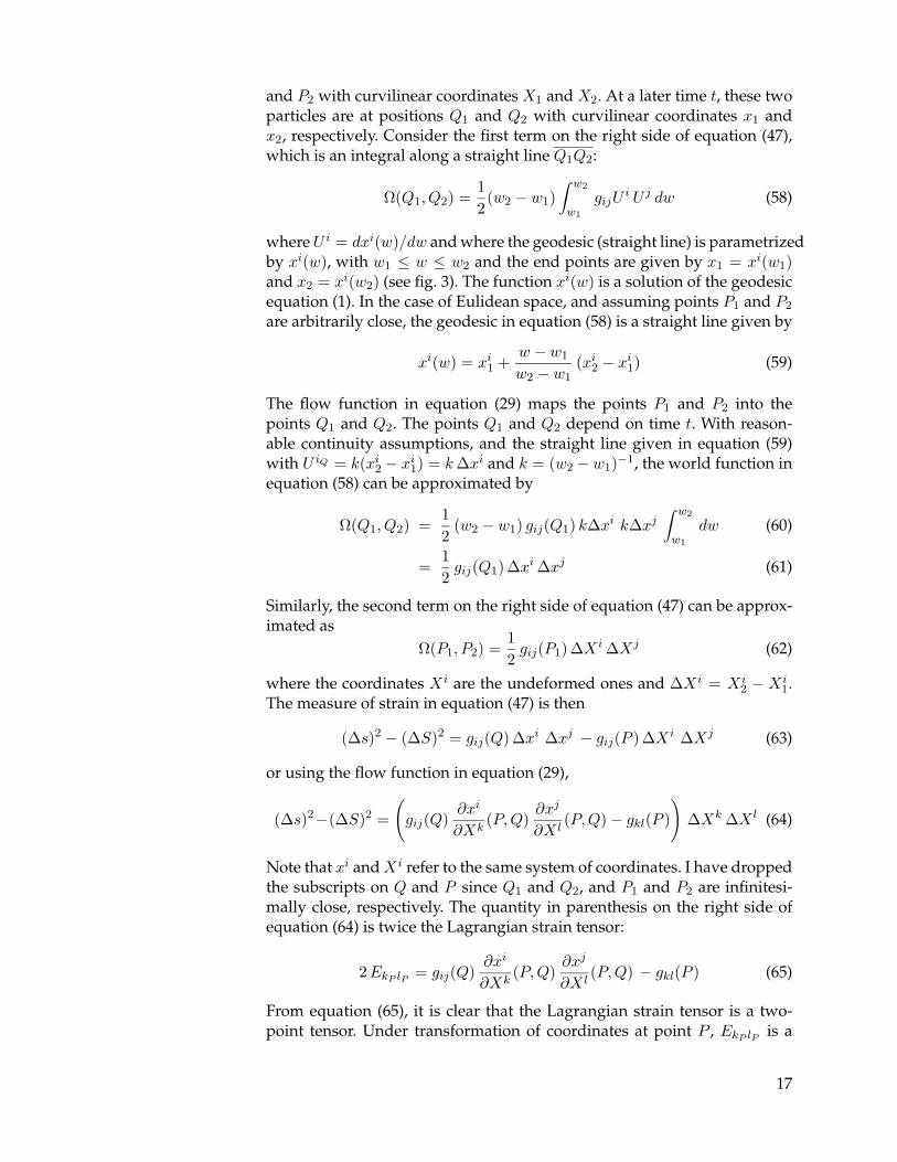
and P2 with curvilinear coordinatesX1 andX2. At a later time t, these twoparticles are at positions Q1 and Q2 with curvilinear coordinates x1 andx2, respectively. Consider the first term on the right side of equation (47),which is an integral along a straight line Q1Q2:

Ω(Q1, Q2) =12(w2 − w1)

∫ w2

w1

gijUi U j dw (58)

whereU i = dxi(w)/dw and where the geodesic (straight line) is parametrizedby xi(w), with w1 ≤ w ≤ w2 and the end points are given by x1 = xi(w1)and x2 = xi(w2) (see fig. 3). The function xi(w) is a solution of the geodesicequation (1). In the case of Eulidean space, and assuming points P1 and P2

are arbitrarily close, the geodesic in equation (58) is a straight line given by

xi(w) = xi1 +

w − w1

w2 − w1(xi

2 − xi1) (59)

The flow function in equation (29) maps the points P1 and P2 into thepoints Q1 and Q2. The points Q1 and Q2 depend on time t. With reason-able continuity assumptions, and the straight line given in equation (59)with U iQ = k(xi

2 − xi1) = k∆xi and k = (w2 −w1)−1, the world function in

equation (58) can be approximated by

Ω(Q1, Q2) =12

(w2 − w1) gij(Q1) k∆xi k∆xj∫ w2

w1

dw (60)

=12gij(Q1) ∆xi ∆xj (61)

Similarly, the second term on the right side of equation (47) can be approx-imated as

Ω(P1, P2) =12gij(P1) ∆Xi ∆Xj (62)

where the coordinates Xi are the undeformed ones and ∆Xi = Xi2 − Xi

1.The measure of strain in equation (47) is then

(∆s)2 − (∆S)2 = gij(Q) ∆xi ∆xj − gij(P ) ∆Xi ∆Xj (63)

or using the flow function in equation (29),

(∆s)2−(∆S)2 =

(gij(Q)

∂xi

∂Xk(P,Q)

∂xj

∂X l(P,Q) − gkl(P )

)∆Xk ∆X l (64)

Note that xi andXi refer to the same system of coordinates. I have droppedthe subscripts on Q and P since Q1 and Q2, and P1 and P2 are infinitesi-mally close, respectively. The quantity in parenthesis on the right side ofequation (64) is twice the Lagrangian strain tensor:

2EkP lP = gij(Q)∂xi

∂Xk(P,Q)

∂xj

∂X l(P,Q) − gkl(P ) (65)

From equation (65), it is clear that the Lagrangian strain tensor is a two-point tensor. Under transformation of coordinates at point P , EkP lP is a

17

second rank tensor, while under transformation of coordinates at point Q,it is a scalar. The deformation gradient, ∂xi/∂Xk, is itself a two-point tensor,as can be seen by its transformation property when coordinates at P andQare changed.

It is interesting to note that the Lagrangian strain tensor Ekl is convention-ally thought to be a function of material coordinates, Xi, which coincidewith the point P (in the reference configuration) [8,9]. The tensor EkP lP canbe taken to be a function of only the material coordinates by using the flowmapping function in equation (29), which provides a mapping between allpoints P and their images, pointsQ, under the deformation. However, I donot pursue this interpretation below.

The first term in equation (65) is the Green deformation tensor:

Ckl = gij(Q)∂xi

∂Xk(P,Q)

∂xj

∂X l(P,Q) (66)

The point P is in the reference configuration at time t = to and the pointQ is in the deformed state at time t. In equation (66), the Green deforma-tion tensor is naturally a second rank tensor with respect to material coor-dinate transformations (point P ) and it is a scalar with respect to spatialcoordinate transformations (point Q). However, the Green tensor is con-ventionally taken [8,9] as a function of material coordinates by using theflow mapping function in equation (29).

Returning to equation (64), and using the flow mapping function in equa-tion (29), we can obtain

(∆s)2 − (∆S)2 =

(gij(Q) − gkl(P )

∂Xk

∂xi(P,Q)

∂X l

∂xj(P,Q)

)∆xi ∆xj (67)

where the Eulerian strain tensor eiQjQ is given by

2 eiQjQ = gij(Q) − gkl(P )∂Xk

∂xi(P )

∂X l

∂xj(P ) (68)

The Eulerian strain tensor eiQjQ is a two-point tensor that is second rankwith respect to spatial coordinates at point Q and is a scalar with respectto material coordinates at point P . Once again, however, using the flowmapping function in equation (29), eiQjQ can be imagined to depend on thematerial coordinates xi (point Q) of the deformed state.

18

5. Strain Tensors in Terms of the Displacement Field

The Eulerian and Lagrangian strain tensors can be expressed in terms ofthe displacement fields uiQ and U iP in equations (40) and (41). In terms ofcovariant components, the displacement field vector at Q is given by

uiQ = ΩiQ(O,Q) − giQjP ΩjP (O,P ) (69)

The covariant derivative of uiQ with respect to point Q (coordinates xk) is

uiQ;kQ= ΩiQkQ

(O,Q) − g jPiQ

ΩjP lP (O,P )∂X l

∂xk(70)

where I used the chain rule for covariant differentiation since Ω(O,P ) =Ω(O,P (X)) and the material coordinates X l = X l(xk) are functions ofthe spatial coordinates xk. It is clear that the chain rule must be used inequation (70) by considering Cartesian coordinates. In equation (70), wealso used the fact that in Euclidean space the parallel propagator is a con-stant under covariant differentiation. The notation ΩiQkQ

(O,Q) means the(i, k) component of the second covariant derivative of the world function atpoint Q. In Euclidean space, these second covariant derivatives are simplyrelated to the parallel propagator (see eqs (21)–(23)).

Using equation (23), the covariant derivative of the displacement field inequation (70) becomes

uiQ;kQ= gik(Q) − g jP

iQgjl(P )

∂X l

∂xk(71)

= gik(Q) − giQlP

∂X l

∂xk(72)

where in the last line the metric at P , gjl(P ), was used to lower the index onthe propagator. Now we multiply equation (72) by the parallel propagatorgmP iQ , sum on iQ, and solve for the inverse displacement gradient

∂Xm

∂xk= gmP

kQ− gmP iQ uiQ;kQ

(73)

From equation (73), it is clear that in Euclidean space, the deformation gra-dient ∂Xm/∂xk is simply related to the covariant derivative of the displace-ment field, uiQ;kQ

. Note however, that in a Riemannian space, for finite de-formations, it is generally not possible to solve for the deformation gradi-ent [18]. Now, using equation (73) in equation (67), we find the expressionrelating the two-point Eulerian strain tensor eiQjQ = eiQjQ(P,Q) to the co-variant derivatives of the three-point displacement field

(∆s)2 − (∆S)2 =[uiQ;jQ + ujQ;iQ − gkl(Q)ukQ;iQ ulQ;jQ

]∆xi ∆xj (74)

= 2 eiQjQ ∆xi ∆xj (75)

19

whereeiQjQ =

12

[uiQ;jQ + ujQ;iQ − gkl(Q)ukQ;iQ ulQ;jQ

](76)

Equation (76) explicitly shows that the Eulerian strain tensor eiQjQ is a func-tion of two points, material coordinates at point P and spatial coordinatesat point Q. Note that eiQjQ is not a function of point O, since by equa-tion (71) the covariant derivative uiQ;jQ does not depend on point O. Fromequation (76) it is also clear that eiQjQ transforms as a second rank tensorunder spatial coordinate transformations and that it transforms as a scalarunder material coordinate transformations.

An analogous relation can be obtained for the Lagrangian strain tensor byconsidering the covariant derivative of the displacement field

UiP ;kP= g

jQ

iPΩjQlQ(O,Q)

∂xl

∂Xk− ΩiP kP

(O,P ) (77)

Using the relations between the second covariant derivatives of the worldfunction and propagator in equations (21)–(23), and solving for the dis-placement gradient we get

∂xm

∂Xk= g

mQ

kP− gmQiP UiP ;kP

(78)

Inserting the displacement gradient in equation (78) into equation (64) givesan expression for the Lagrangian strain tensor EmP nP = EmP nP (P,Q),

(∆s)2 − (∆S)2 =[UmP ;nP + UnP ;mP + gij(P )UiP ;mP UjP ;nP

]∆Xm ∆Xn (79)

= 2EmP nP ∆Xi ∆Xj (80)

where

EmP nP =12

[UmP ;nP + UnP ;mP + gij(P )UiP ;mP UjP ;nP

](81)

Equation (79) shows that the Lagrangian strain tensor EmP nP is a functionof the material coordinates at point P and spatial coordinates at point Q.The Lagrangian strain tensor transforms as a scalar under spatial coordi-nate transformations at pointQ and as a second rank tensor with respect tomaterial coordinate transformations at point P . Note that there are sign dif-ferences in equations (76) and (81). Finally, comparing equations (74) and(79), we have the well-known relation between the two strain tensors

EmP nP = eiQjQ

∂xi

∂Xm

∂xj

∂Xn(82)

Equation (82) provides a complicated relation between the two two-pointstrain tensors. While the displacement fields uiQ and U iP are related to eachother by parallel transport (see eqs (40) and (41)), the strain tensors EmP nP

and eiQjQ are related by two-point deformation gradient tensors, ∂xi/∂Xm,in equation (82).

20

6. Summary

Conventionally, the Eulerian and Lagrangian strain tensors are derived ei-ther by using shifter tensors or by using convected (moving) coordinates.The definition of the shifter tensor makes use of a scalar product betweenvectors at two different points in space (without first parallel translatingone vector to the position of the other). When convected coordinates areused, vectors and tensors are associated with given coordinates in the con-vected system of coordinates, rather than being associated with a givenpoint in the underlying space. As discussed in the introduction, both ofthese features are undesireable when we need to understand the transfor-mation properties of the strain tensors from an inertial frame to a movingframe. These transformation properties are also needed in order to gener-alize the strain tensor to Riemannian geometry for applications to generalrelativity.

I have provided a derivation of the Eulerian and Lagrangian strain tensorsfor finite deformations using the concepts of parallel propagator, the worldfunction of J. L. Synge and the three-point displacement vector field. Thisderivation avoids the undesireable features mentioned above. The deriva-tion shows that the Eulerian strain tensor is a two-point object that trans-forms as a scalar under transformation of material coordinates and as a sec-ond rank tensor under transformation of spatial coordinates. The deriva-tion also shows that the Lagrangian strain tensor behaves as a scalar undertransformation of spatial coordinates and as a second rank tensor undertransformation of material coordinates. These transformation propertiesare useful in understanding how these strain tensors transform from oneframe of reference to another moving, non-inertial frame. The formulationpresented here of the transformation properties of these tensors is also use-ful for understanding the role of the reference (unstrained) configuration inprestressed materials, as discussed in the introduction.

21

Acknowledgments

The author thanks Dr. W. C. McCorkle, U. S. Army Aviation and MissileCommand, for suggesting investigation of the problem of stresses in a ro-tating cylinder, which relied on the ideas in this manuscript as a conceptualfoundation.

22

References

1. A. E. H. Love, A Treatise on the Mathematical Theory of Elasticity, DoverPublications, 4th Edition, New York, (1944), p. 148.

2. L. D. Landau and E. M. Lifshitz, Theory of Elasticity, Pergamon Press,New York (1970), p. 22.

3. A. Nadai, “Theory of Flow and Fracture of Solids,” McGraw-Hill,New York (1950), p. 487.

4. E. E. Sechler, Elasticity in Engineering, John Wiley & Sons, Inc., NewYork (1952), p. 164.

5. S. P. Timoshenko and J. N. Goodier, Theory of Elasticity, 3rd Edition,McGraw-Hill Book Company, New York, (1970), p. 81.

6. E. Volterra and J. H. Gaines, Advanced Strength of Materials, Prentice-Hall, Inc., Englewood Cliffs, N.J., USA, (1971), p. 156.

7. T. B. Bahder, “Stress in Rotating Disks and Cylinders,” US Army Re-search Laboratory, ARL-TR-2576.

8. A. C. Eringen, Nonlinear Theory of Continuous Media, McGraw-HillBook Company, New York, (1962).

9. M. N. L. Narasimhan, Principles of Continuum Mechanics, John Wiley& Sons, Inc., New York (1992).

10. W. C. McCorkle, “Compensated Pulsed Alternators to Power Electro-magnetic Railguns,” 12th IEEE International Pulsed Power Confer-ence 1999, vol. I (1999), p. 364–368.

11. F. D. Murnaghan, American Journ. Math., “Finite Deformations of anElastic Solid,” 59 (1937), 235–260.

12. A. E. Green and W. Zerna, Theoretical Elasticity, Oxford (1954).

13. I. S. Sokolnokoff, Tensor Analysis: Theory and Applications to Geometryand Mechanics of Continua, Second Edition, John Wiley & Sons, Inc.,New York (1964).

14. W. Flugge, Tensor Analysis and Continuum Mechanics, Springer-Verlag,New York (1972).

15. J. L. Ericksen, “Tensor Fields,” in Appendix of C. Truesdell and R.Toupin “The Classical Field Theories,” in “Handbuch der Physik,”vol. III, Part 1, Springer-Verlag, Berlin (1960).

23

16. J. L. Synge, Relativity: The General Theory (North-Holland PublishingCo., New York, 1960).

17. G. A. Maugin, “Harmonic Oscillations of Elastic Continua and Detec-tion of Gravitational Waves,” Gen. Rel. Grav. 3, (1973), 241–272.

18. J. M. Gambi, A. San Miguel, and F. Vicente, Gen. Rel. Grav., “The Rel-ative Deformation Tensor for Small Displacements in General Relativ-ity,” 21, (1989), 279–286.

19. J. L. Synge and A. Schild, Tensor Calculus, Dover Publications, NewYork (1949).

20. See A. C. Eringen, in Continuum Physics, Ed. by A. C. Eringen, Aca-demic Press, New York (1971).

21. H. S. Ruse, “Taylor’s Theorem in the Tensor Calculus,” Proc. LondonMath. Soc. 32, (1931), 87–92.

22. H. S. Ruse, “An Absolute Partial Differential Calculus,” Quart. J.Math. Oxford Ser. 2, (1931), 190.

23. J. L. Synge, “A Characteristic Function in Riemannian Space andits Application to the Solution of Geodesic Triangles,” Proc. LondonMath. Soc. 32, (1931), 241–258.

24. K. Yano and Y. Muto, “Notes on the deviation of geodesics and thefundamental scalar in a Riemannian space,” Proc. Phys.-Math. Soc.Jap. 18, (1936), 142.

25. J. A. Schouten, Ricci-Calculus. An Introduction to Tensor Analysis and ItsGeometrical Applications, (Springer-Verlag, 2nd ed., 1954).

26. T. B. Bahder, “Navigation in curved space-time,” Am. J. Physics, 69,(2001), 315.

27. R. W. John, “Zur Berechnung des geodatischen Abstands und as-soziierter Invarianten im relativistischen Gravitationsfeld,” Ann. derPhys. Lpz. 41, (1984), 67–80.

28. R. W. John, “The world function of space-time: some explicit exactresults for specific metrics,” Ann. der Phys. Lpz. 41, (1989), 58–70.

29. H. A. Buchdahl and N. P. Warner, “On the world function of theSchwarzschild field,” Gen. Rel. and Grav. 10, (1979), 911–923.

30. J. Kraus, Int. J. Theor. Phys. 12, (1975), 35.

24

31. A. J. M. Spencer, Continuum Mechanics, Longman Mathematical Texts,Longman, New York (1980), p. 63.

32. J. M. Gambi, P. Romero, A. San Miguel, and F. Vicente, “Fermi coor-dinate transformation under baseline change in relativistic celestialmechanics,” International J. Theor. Phys. 30, (1991), 1097–1116.

25

27

Distribution

AdmnstrDefns Techl Info CtrATTN DTIC-OCP8725 John J Kingman Rd Ste 0944FT Belvoir VA 22060-6218

DARPAATTN S Welby3701 N Fairfax DrArlington VA 22203-1714

Defns Mapping AgcyATTN L-41 B HaganATTN L-41 D Morgan3200 S 2nd StretST Louis MO 63118

Ofc of the Secy of DefnsATTN ODDRE (R&AT)The PentagonWashington DC 20301-3080

AMCOM MRDECATTN AMSMI-RD W C McCorkleRedstone Arsenal AL 35898-5240

US Military AcdmyMathematical Sci Ctr of ExcellenceATTN MADN-MATH MAJ M JohnsonThayer HallWest Point NY 10996-1786

US Army ARDECATTN AMSTA-AR-TDBldg 1Picatinny Arsenal NJ 07806-5000

US Army Info Sys Engrg CmndATTN AMSEL-IE-TD F JeniaFT Huachuca AZ 85613-5300

US Army MICOMATTN AMSMI-RD-MG-NC G GrahamRedstone Arsenal AL 35898-5254

US Army Mis Cmnd Weapons Sci DirctrtATTN AMSMI-RD-WS-ST C M BowdenRedstone Arsenal AL 35898-5358

US Army Tank-Automtv Cmnd RDECATTN AMSTA-TR J ChapinWarren MI 48397-5000

Ofc of Nav RsrchATTN ONR 331 H Pilloff800 N Quincy StretArlington VA 22217

Univ of Texas at Austin Inst for AdvancedTech

ATTN I Mcnab4030-2 West Braker LnAustin TX 78759-5329

Meta RsrchATTN T Van Flandern6327 Western Ave NWWashington DC 20015

US Army Rsrch LabATTN AMSRL-WM-TE C HummerBldg 120Aberdeen Proving Ground MD 21005-5066

DirectorUS Army Rsrch LabATTN AMSRL-RO-D JCI ChangATTN AMSRL-RO-P H EverittPO Box 12211Research Triangle Park NC 27709

US Army Rsrch LabATTN AMSRL-RO M StroscioPO Box 12211Research Triangle Park NC 27709-2211

US Army Rsrch LabATTN AMSRL-CI-IS-R Mail & Records MgmtATTN AMSRL-CI-IS-T Techl Pub (2 copies)ATTN AMSRL-CI-OK-TL Techl Lib (2 copies)ATTN AMSRL-D R W WhalinATTN AMSRL-SE J PellegrinoATTN AMSRL-SE-DP H BrandtATTN AMSRL-SE-E G SimonisATTN AMSRL-SE-E H PollehnATTN AMSRL-SE-EE T B Bahder (40 copies)

Distribution (cont’d)

28

US Army Rsrch Lab (cont’d)ATTN AMSRL-SE-EE Z G SztankayATTN AMSRL-SE-EP J Bruno

US Army Rsrch Lab (cont’d)ATTN AMSRL-SE-SA J EickeAdelphi MD 20783-1197

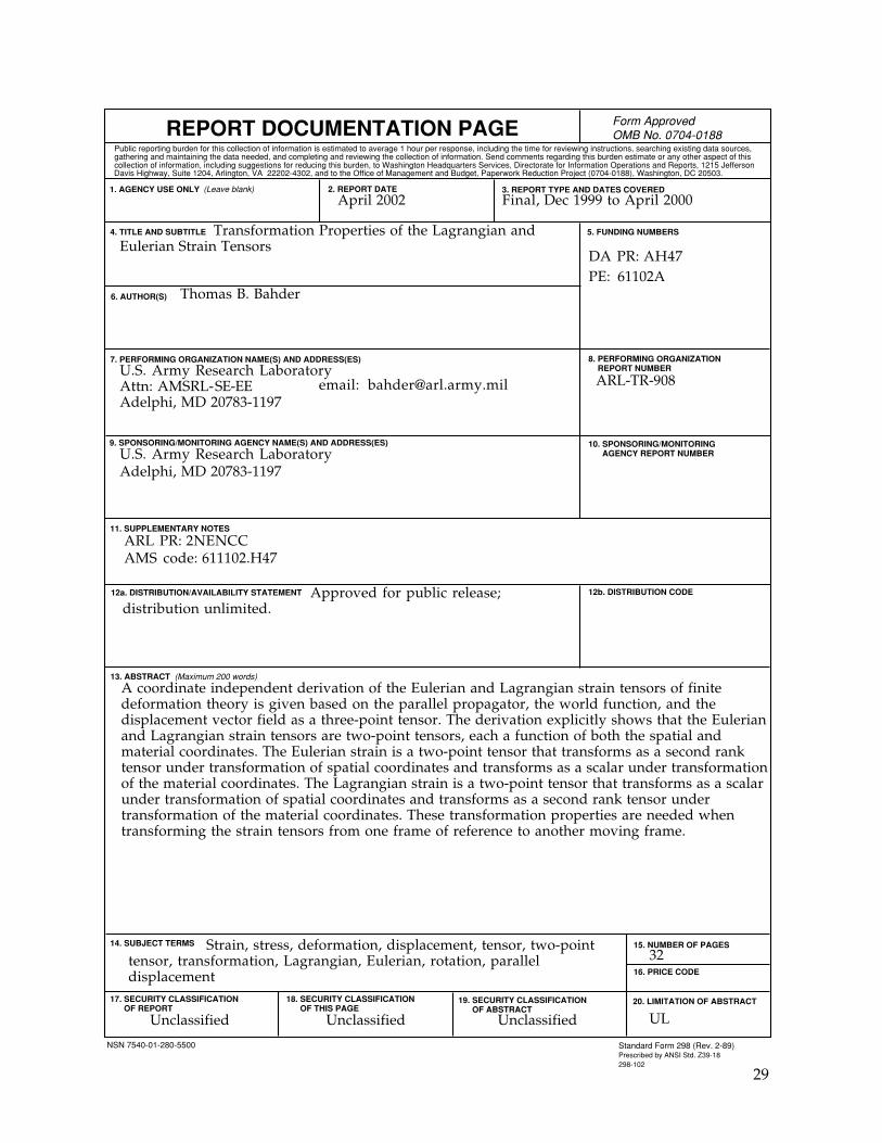
1. AGENCY USE ONLY

8. PERFORMING ORGANIZATION REPORT NUMBER

7. PERFORMING ORGANIZATION NAME(S) AND ADDRESS(ES)

12a. DISTRIBUTION/AVAILABILITY STATEMENT

10. SPONSORING/MONITORING AGENCY REPORT NUMBER

5. FUNDING NUMBERS4. TITLE AND SUBTITLE

6. AUTHOR(S)

REPORT DOCUMENTATION PAGE

3. REPORT TYPE AND DATES COVERED2. REPORT DATE

11. SUPPLEMENTARY NOTES

14. SUBJECT TERMS

13. ABSTRACT (Maximum 200 words)

Form ApprovedOMB No. 0704-0188

(Leave blank)

9. SPONSORING/MONITORING AGENCY NAME(S) AND ADDRESS(ES)

Public reporting burden for this collection of information is estimated to average 1 hour per response, including the time for reviewing instructions, searching existing data sources,gathering and maintaining the data needed, and completing and reviewing the collection of information. Send comments regarding this burden estimate or any other aspect of thiscollection of information, including suggestions for reducing this burden, to Washington Headquarters Services, Directorate for Information Operations and Reports, 1215 JeffersonDavis Highway, Suite 1204, Arlington, VA 22202-4302, and to the Office of Management and Budget, Paperwork Reduction Project (0704-0188), Washington, DC 20503.

12b. DISTRIBUTION CODE

15. NUMBER OF PAGES

16. PRICE CODE

17. SECURITY CLASSIFICATION OF REPORT

18. SECURITY CLASSIFICATION OF THIS PAGE

19. SECURITY CLASSIFICATION OF ABSTRACT

20. LIMITATION OF ABSTRACT

NSN 7540-01-280-5500 Standard Form 298 (Rev. 2-89)Prescribed by ANSI Std. Z39-18298-102

Transformation Properties of the Lagrangian andEulerian Strain Tensors

April 2002 Final, Dec 1999 to April 2000

A coordinate independent derivation of the Eulerian and Lagrangian strain tensors of finitedeformation theory is given based on the parallel propagator, the world function, and thedisplacement vector field as a three-point tensor. The derivation explicitly shows that the Eulerianand Lagrangian strain tensors are two-point tensors, each a function of both the spatial andmaterial coordinates. The Eulerian strain is a two-point tensor that transforms as a second ranktensor under transformation of spatial coordinates and transforms as a scalar under transformationof the material coordinates. The Lagrangian strain is a two-point tensor that transforms as a scalarunder transformation of spatial coordinates and transforms as a second rank tensor undertransformation of the material coordinates. These transformation properties are needed whentransforming the strain tensors from one frame of reference to another moving frame.

Strain, stress, deformation, displacement, tensor, two-pointtensor, transformation, Lagrangian, Eulerian, rotation, paralleldisplacement

Unclassified

ARL-TR-908

2NENCC611102.H47

AH4761102A

ARL PR:AMS code:

DA PR:PE:

Approved for public release;distribution unlimited.

32

Unclassified Unclassified UL

Adelphi, MD 20783-1197

U.S. Army Research LaboratoryAttn: AMSRL-SE-EE bahder@arl.army.mil

U.S. Army Research Laboratory

29

Thomas B. Bahder

email:Adelphi, MD 20783-1197