trajectory optimization and real-time simulation for ... optimization and real-time simulation ......
TRANSCRIPT

Trajectory optimization and real-time simulation for robotics applications
Michele AttolicoPierangelo MasaratiPaolo Mantegazza
Dipartimento di Ingegneria AerospazialePolitecnico di Milano
Multibody Dynamics 2005International Conference on Advances in Computational Multibody DynamicsECCOMAS Thematic Conference
Madrid, June 2005

M. AttolicoP. MasaratiP. Mantegazza
1. The trajectory optimization problem.
2. A description of MBDyn.
3. Application
4. The real-time simulation.
Index

M. AttolicoP. MasaratiP. Mantegazza
The dynamic equations
The multi-body equations of the robot are:
where:• and are the states
• and are the system inputs
F x t , x t , z t ,u t , p=0G x t , p=0
x t z t
u t p

M. AttolicoP. MasaratiP. Mantegazza
The trajectory optimization problem
Find a control input and a value in order to move the robot :
● Minimizing a suitable cost function.
● Satisfying some constraints over the trajectory:
Finalposition
Initialposition
C x t ,u t , p0
u t p

M. AttolicoP. MasaratiP. Mantegazza
The trajectory optimization problem
The cost function has the form:
where
and is the impulse response of a suitable filter .
In this work, a high pass filter is used, in order to have a controllaw with reduced energy at high frequency.
f u t ,T =∫0
T
d 1d 2v t T v t dt
v t =∫0
t
w t−u dt
w t W s

M. AttolicoP. MasaratiP. Mantegazza
From the continuous to the discrete problem
A direct method is used:
• The system input must be discretized over a time grid:• The discrete values become unknowns of the optimization problem• The continuous behavior is obtained by polynomial interpolation.
The interpolation order can change at each time interval.• The dynamics equations are integrated by MBDyn multi-body solver
through a “shooting” procedure
• The constraints are sampled:• Any continuous constraint generates many discrete constraints at
different times.• Not all the integration times can be used because the problem
becomes too large.• An heuristic algorithm selects only those times where the
constraints are about to be violated.
u t
C x t ,u t , p0

M. AttolicoP. MasaratiP. Mantegazza
From the continuous to the discrete problem
The problem unknowns are:• the final time T• the discrete values of the j-th control input• the constant system input p
y={T⋮u j⋮p}
u j

M. AttolicoP. MasaratiP. Mantegazza
From the continuous to the discrete problem
An SQP algorithm is used to solve the optimal problem:• Harwell VF13 solver• Iterative solution• The following differential quantities are needed:
– – the constraints Jacobian
The derivatives are computed through central finite difference:• 2n+1 dynamic equations integrations are needed at each
optimization step, where n is the unknowns number.
∇ fJ

M. AttolicoP. MasaratiP. Mantegazza
The optimization algorithm
MBDyn Assembler
VF13 solver
f ,∇ f ,C , Jy
u t , p ,T
x t

M. AttolicoP. MasaratiP. Mantegazza
The optimization algorithm
MBDyn Assembler
VF13 solver
f ,∇ f ,C , Jy
u t , p ,T
x t Optimizer program

M. AttolicoP. MasaratiP. Mantegazza
Problem adaptation
When an optimal solution is found, a problem adaptation can beperformed:
The control are adapted:• some interpolation points are inserted or deleted in the
discretization grid• the most appropriate polynomial interpolation function is selected in
a given interval of the analysis timeA new optimization can be performed starting from the formersolution
u t

M. AttolicoP. MasaratiP. Mantegazza
MBDyn Overview
Index 2/3 Differential-Algebraic, Initial-Value problem solver
Algebraic kinematic constraints; e.g.– revolute joints
Multidisciplinary problems capability:– aeroelasticity– electric components– hydraulic components
Implicit integration by means of second-order A/L stable scheme
M x−=0−F x , x ,t =0
x , x ,t =0

M. AttolicoP. MasaratiP. Mantegazza
MBDyn Overview
Free software project:
http://www.aero.polimi.it/~mbdyn/
Developed at the “Dipartimento di Ingegneria Aerospaziale”of the University “Politecnico di Milano”
General purpose:• parallel/multithread linear/nonlinear solvers• distributed Real-Time enabled by RTAI/RT-Net/RTAILab• interface to arbitrary CFD solvers for aeroelastic analysis

M. AttolicoP. MasaratiP. Mantegazza
Algorithm validation
The validation has been made by means ofproblems with analytical solutions:
– Material point linear movement thrust through a force, with various constraints.
– The found solutions agree with the analytical ones

M. AttolicoP. MasaratiP. Mantegazza
Application:Two arms robot
The robotic arm is a two degree of freedom planar robot
The system inputs are the couples , applied at the two hinges. The couples can vary between -1 and 1 whereas the hinge angles , between -135 and 135 degrees
C 1
1
C 2
2

M. AttolicoP. MasaratiP. Mantegazza
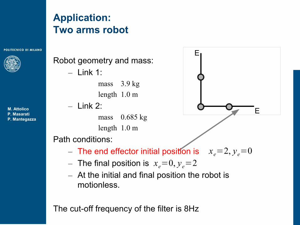
Application:Two arms robot
Robot geometry and mass:– Link 1:
mass 3.9 kglength 1.0 m
– Link 2:mass 0.685 kglength 1.0 m
Path conditions:– The end effector initial position is– The final position is– At the initial and final position the robot is
motionless.
The cut-off frequency of the filter is 8Hz
xe=0, ye=2
E
E
xe=2, ye=0
M. AttolicoP. MasaratiP. Mantegazza
Application:Two arms robot
Robot geometry and mass:– Link 1:
mass 3.9 kglength 1.0 m
– Link 2:mass 0.685 kglength 1.0 m
Path conditions:– The end effector initial position is– The final position is– At the initial and final position the robot is
motionless.
The cut-off frequency of the filter is 8Hz
E
E
xe=0, ye=2xe=2, ye=0

M. AttolicoP. MasaratiP. Mantegazza
Application:Two arms robot
Results:– The optimal solution is found after:
• 233 iterations• 16633 MBDyn runs• 5 control adaptations
– The traveling time is 3.436s

M. AttolicoP. MasaratiP. Mantegazza
Application:Two arms robot
The hinge angles are:

M. AttolicoP. MasaratiP. Mantegazza
Application:Two arms robot
... and the resulting path is:

M. AttolicoP. MasaratiP. Mantegazza
Application:Two arms robot
Then the optimal solution is proved with a moresophisticated model:
– The two link are flexible:• First link: iron, thickness 5.0mm• Second link: aluminium alloy, thickness 2.5mm
– A feedback control is needed:• The torque applied at each hinge becomes the
sum of the feedback control output and the optimal solution

M. AttolicoP. MasaratiP. Mantegazza
Application:Two arms robot

M. AttolicoP. MasaratiP. Mantegazza
Application:Two arms robot

M. AttolicoP. MasaratiP. Mantegazza
Application:Two arms robot

M. AttolicoP. MasaratiP. Mantegazza
Application:Two arms robot

M. AttolicoP. MasaratiP. Mantegazza
Application:Two arms robot

M. AttolicoP. MasaratiP. Mantegazza
Real-Time Simulation
MBDyn allows real-time simulation under LinuxReal-Time Application Interface (RTAI) http://www.rtai.org/
Advantages:– same software for rather different purposes– same models/model components; no modeling limitations
Drawbacks:– “large” models (redundant set) => sample rate limitations– no theoretical guaranteed upper bound to worst case time
Good performances obtained so far– 6 dof robot with friction, 120 eq.: >2 kHz on Athlon 2.4 GHz

M. AttolicoP. MasaratiP. Mantegazza
Real-Time Simulation (cont.)
Distributed Real-Time simulation:– Multibody Analysis– Control– Monitoring
\

M. AttolicoP. MasaratiP. Mantegazza
Conclusions
The optimization using a MBDyn software is a powerful and versatile tool.
It is possible to verify the optimal solution with the same model in a complete control scheme
Further development:•Optimization with flexible models