training manual - grid - unep
TRANSCRIPT

Risk and Vulnerability Assessment Methodology Development Project (RiVAMP)
Training Manual
G R I DG e n e v a
2012
Quantifying the role of marine and coastal ecosystems in mitigating beach erosion

2
UNEP/GRID-Geneva Global Change & Vulnerability Unit 11, ch. Des Anémones 1219 Châtelaine Geneva – Switzerland Tel: +4122.917.82.94 Fax: +4122.917.80.29 Website: www.grid.unep.ch
Lead Authors
Bruno Chatenoux, Pascal Peduzzi, Adonis Velegrakis
Citation
Chatenoux, B., Peduzzi, P., Velegrakis, V. (2012), RIVAMP training on the role of Coastal and Marine ecosystems for mitigating beach erosion : the case of Negril Jamaica, UNEP/GRID-Geneva, Geneva, Switzerland.
UNEP 2012
DisclaimerThe designations employed and the presentation of material on the maps do not imply the expression of any opinion whatsoever on the part of UNEP or the Secretariat of the United Nations concerning the legal status of any country, territory, city or area or of its authorities, or concerning the delimitation of its frontiers or boundaries. UNEP and collaborators should in no case be liable for misuse of the presented results. The views expressed in this publication are those of the authors and do not necessarily reflect those of UNEP. Acknowledgements This research would not have been possible without the close collaboration of the Planning Institute of Jamaica (PIOJ) and the Division of Environment Division of Environmental Policy Implementation (DEPI).
3
Table of Contents Introduction ........................................................................................................................4 RiVAMP GIS Training ........................................................................................................5
In brief ............................................................................................................................5 Typographic convention .................................................................................................5 QGIS and GRASS installation ........................................................................................5 Before to start .................................................................................................................6 Customizing QGIS ..........................................................................................................6 Introduction to QGIS .......................................................................................................9 Population distribution ..................................................................................................13
Load and explore the data ........................................................................................13 Generate the population distribution raster ...............................................................13
Bathymetry ...................................................................................................................17 Interpolate a raster from contour lines .......................................................................17
Flooded area exposure.................................................................................................19 Identify the flooded areas ..........................................................................................19 Compute the exposure..............................................................................................21
Profile extraction...........................................................................................................23 Draw the profiles .......................................................................................................23
Plugins selection ..........................................................................................................30 References ...................................................................................................................30 Index ............................................................................................................................30
RiVAMP statistical analysis Training ................................................................................31 Some theory .................................................................................................................31
Statistical concepts ...................................................................................................31 Multiple regression analysis ......................................................................................31 Pearson coefficient, r ................................................................................................31 R2 and Adjusted R2 ...................................................................................................32 Normal distribution ....................................................................................................32 Correlation matrix .....................................................................................................33 Outliers .....................................................................................................................33 Causality ...................................................................................................................33 What is a good model? .............................................................................................35
In brief ..........................................................................................................................36 Typographic convention ...............................................................................................36 TANAGRA installation (if necessary) ............................................................................36 Introduction to TANAGRA ............................................................................................36 Data preparation and importation in TANAGRA ...........................................................37 Explore the dataset ......................................................................................................38 Clarify ideas through automatic regression ...................................................................39 Increase the dataset .....................................................................................................40 Repeat the data exploration and automatic regression .................................................40 Precise manually the model through manual iterations .................................................40 Improve the model by removing outliers .......................................................................41
Database of Beach Retreat Projections and Beach Retreat Estimators ...........................43 Introduction ..................................................................................................................43 Beach retreat morphodynamic models .........................................................................43 Introduction to Matlab GUI ............................................................................................47 Database of Beach Retreat Projections ........................................................................48 Beach Retreat Estimator ..............................................................................................66 References ...................................................................................................................80
Beach Retreat under Sea Level Rise ...............................................................................81 References ...................................................................................................................82

4
Introduction The Risk and Vulnerability Assessment Methodology Development Project (RiVAMP) is a
collaboration between the United Nations Environment Programme Division of Early Warning and Assessment (DEWA) and Division of Environmental Policy Implementation (DEPI) and aims to identify and quantify the role of ecosystems in Disaster Risk Reduction (DRR) and climate change adaptation (CCA).
Such methodology can be applied in different ecosystems, this one is tailored to the role of coastal and marine ecosystems in mitigating beach erosion, thus reducing impacts from storm surges generated by tropical cyclones and the impacts from sea level rise. This is more specifically targeting for Small Islands Developing States (SIDS).
The pilot study was carried out in Jamaica and concentrate on beach erosion in Negril area (at the request of the Jamaican government). The methodology includes local experts and community consultations integrated with spatial analysis (GIS and remote sensing), erosion modelling and statistical analysis.
The assessment tool was pilot tested in Jamaica, as a small island developing state. The national partner was the Planning Institute of Jamaica (PIOJ). According to the IPCC’s Fourth Assessment Report, global climate change will particularly impact on small island developing states (SIDS), such as Jamaica, which have a high coastal population density and existing vulnerability to natural hazards. The importance of nature-based tourism and climate sensitive livelihoods (agriculture and fisheries) in Jamaica make it critical to understand changing patterns of risk and develop effective response.
Following the release of the RiVAMP study results, the government of Jamaica, through PIOJ, requested UNEP to get a transfer of this methodology to Jamaican scientists. DEWA financed the creation of the training manual, including the transfer of the methodology on free OpenSource software (to avoid creating dependencies) and DEPI/PCDMB financed the mission itself.
In agreement with the Jamaican government, we are pleased to provide access to this training on-line, so that anybody who is interested in quantifying the role of ecosystems can access such training and related tools (GIS, statistics and beach erosion modelling software).
This training document has been created by Bruno Chatenoux (UNEP/DEWA/GRID-Geneva) – GIS chapter, Pascal Peduzzi (UNEP/DEWA/GRID-Geneva) – Statistical analysis chapter and Adonis Velegrakis (University of the Aegean) – Hydrology chapter.

5
RiVAMP GIS Training
In brief The aim of this training is to introduce you to the potential of open source applications in
the context of a study such as RiVAMP GIS analysis. To do so the training has been divided into sessions during which you will learn how to practically apply the RiVAMP methodology step by step.
The open source GIS software Quantum GIS 1.7.0 (QGIS) will be used (without using GRASS 6.4.1 even if it will be installed jointly) and the worksheet editor of LibreOffice (fork of OpenOffice).
The training documentation has been prepared under a Windows XP environment, but is easily reproducible in any other OS after a few adjustments (installation, paths). Administrator privileges are required.
Typographic convention In a general manner the text you have to focus because it figures in the applications or
you have to type has been highlighted with Bold Italic format. They constitute the technical skeleton of the process
Menu > Item Instructs you to select the named item from the named menu. Note that some menus contains sub-menus. For example Start > All programs > Quantum GIS Wroclaw > Quantum GIS (1.7.0) is equivalent to the figure below:
>> instructs you to look on the figure on the right for the parameters to be applied.
QGIS and GRASS installation QGIS and GRASS can be installed at
once, including a plugin that will connect them. To do so simply download and install the Windows Standalone Installer from http://www.qgis.org/wiki/Download (also available in the Software folder of the training DVD) using the default options and without adding components. Shortcuts will be created on the Desktop and Windows main menu.
6
Before to start Copy locally (in you computer) the content of the training DVD and look at the way the
data are organised. In the Documents folder you will find the digital version of this documents as well as other
relevant documentation. In the Software folder you will find the installation files for QGIS and LibreOffice, as well
as some files potentially useful. In the GIS folder are located the data you will need during the training. The subfolders are
organised by session, Coordinate Reference System (CRS, equivalent to projection) and data type.
The folder GIS_correction is equivalent to the GIS folder but once the training has been completed in the case you missed one session or would like to compare your results.
Customizing QGIS Start QGIS, by default you get a QGIS Tips! window every time you start the application.
Even if it is a good source of information you can switch it off by checking the I’ve had enough tips,… checkbox to remove it from the start up.
The QGIS graphical interface is divided in 5 zones:
1 Menu bar, 2 Toolbars facilitate the access
to the different functions (also available in the menu bar),
3 Table of Content (ToC) to manage the layers,
4 View, where you can interact with the map,
5 Status bar where you can see information such as coordinates of the pointer, extent, scale, coordinate system; start/stop rendering or define how the view is displayed.
Toolbars are divided by thematic (greyed icons means they are inactive because the
appropriate conditions to use them are not fulfilled). Some of them are included by default in QGIS, some others can be added/removed from the interface:
File
Manage Layers
Map Navigation
Attributes
Label
Raster

7
Digitizing
GRASS plugin
Advanced Digitization
Plugins
We will not describe here the functionalities of each function, some of them will be used
during this training, and you will discover the remaining one on your own as long as you practice.
The toolbars can be added/removed from the interface by right clicking in any empty area of any toolbar or menu and enable/disable them. They can also be moved using drag and drop. The Figure on the right shows the way I generally organize my interface in order too keep it functional. Even if it fits my personal needs, try to get something similar and you will improve it little by little.
Once you get something satisfying, close QGIS and start it again, as you can see the interface remains as you arranged it.
You can see the plugin toolbar remains quite overcrowded, let’s remove the plugins that
we will not need frequently:
Plugins > Manage Plugins…, Uncheck the unnecessary plugins (see the following list with the plugins I generally keep): Add Delimited Text Layer, CopyrightLabel, NorthArrow, Plugin Installer, ScaleBar, fTools.
The disabled plugins will remain installed in QGIS, where they can be activated when
needed (do not hesitate to use the Filter function to find more easily the plugin you are looking for). The enabled plugins will be available through the Plugins menu or specific menu some other through the Plugin toolbar.
Take some time to discover the various functions available through the interface. We just saw how to enable or disable the plugins installed by default in QGIS, lets see
now how we can add more functionalities:
Plugins > Fetch Python Plugins…, Have a quick look at the official plugins available (6 at the time of writing this document), Move to the Repositories tab, click the Add 3rd party repositories button, and accept
the disclaimer window (do not worry if you can not fetch all repositories, it happens some times).

8
Move to the Options tab, and check the Show all plugins, even those marked as experimental radio button (even if “unsecure” this option is necessary at the time of writing this document to get all the functionalities for the Raster menu),
Move back to the Plugins tab and notice you have now more than 170 plugins available and the GdalTools is now upgradable,
You can upgrade it simply by selecting it and clicking the Upgrade plugin button (you do not need to restart QGIS yet as requested).
Have a quick look at the plugins available and try to install the Interactive Identify plugin using the Filter,
Close the window.
Before to go further we need to complete
the Raster menu, by enabling the GdalTools plugin!!!
Notice how the plugins have been
installed on the Plugins menu and toolbar. Each plugin displays differently in QGIS interface, then sometime you will have to search for them!
To complete this chapter let’s customize a bit the QGIS Options the way (in my personal
opinion) they should be by default: Settings > Options…, General tab: check Display classification attribute names in legend, Map tools tab: set the Mouse wheel action to Zoom to mouse cursor, Digitizing tab: check Show markers only for selected features, CRS tab: select EPSG:3448 - JAD2001 / Jamaica Metric Grid (supposing you are
mainly working in Jamaica) as the Default Coordinate System for new projects, check the Enable ‘on the fly’ reprojection by default, and set the Prompt for CRS radio button,
In the case the default interface language is not the appropriate one, you can Override system local (in other words change the interface language) in the Locale tab (this change will be applied the next time you start the application).
Finally press the OK button and close QGIS.

9
Introduction to QGIS This session will quickly present the QGIS interface and functionalities. Do not hesitate to
explore the interface and discover by yourself the different menus and tools available. Start QGIS again and notice how the default coordinate system has been set to
EPSG:3448 (on the right of the status bar). In the case you need to change the coordinate
system, you can press the button (or Settings > Project Properties). Now let’s open some layers:
Layer > Add Vector Layer… (or ), Click the Browse button, Set the Files of type to ESRI Shapefiles [OGR], Select the 3 OSM_*.shp files (using the Shift button) in ...\GIS\1_Introduction\JAD2001\Vector
and click the Open button twice. The 3 layers your added are issued from OpenStreetMap project
(http://www.openstreetmap.org/) and have been downloaded for the all Jamaica from http://downloads.cloudmade.com/americas/caribbean/jamaica (jamaica.shapefiles.zip).
Add now a polygon layers containing the 2nd level administrative extent of Jamaica
(http://www.unsalb.org/): …\GIS\1_Introduction\WGS84\Vector\jam_salb_jan00-aug09.shp. As the polygon layer hide the others layers, drag
and drop it to the bottom of the Table of Content (ToC). Explore for a while the context menu of the layers in
the ToC (right click), visualizing the attribute table and customizing the way the layers are displayed through the Properties.
Try to get something similar to the figure below.

10
Here are some guidelines: Open the Properties of a layer (double click in the ToC), you can rename it in the
tab. While you are here look at the CRS of each layer and notice the efficiency of the “on the fly” reprojection.
You can change the way the layers display with the tab. In the same tab you can Categorize the Highway layer per TYPE, and create a New
color ramp (do not forget to press the Classify button each time you change a Style parameter!).
You can use SVG marker (or fill) through the Change buttons.
As an exercise you can display the Administrative Units labels through the tab (do not forget to check the Display labels checkbox.
What do you think about the result? I personally get frustrated by the way the labels are
displayed. For this reason I prefer to use the Label toolbar: Uncheck the Display labels box in the Administrative Units Properties if necessary,
Then click on the button on the plugin toolbar (enable the plugin if necessary) when the Administrative Units layer is selected,

11
Set the label parameters.
Do not forget to save you project very often!
Let’s add a raster layer now (Digital Elevation Model from SRTM):
Layer > Add Raster Layer… (or ), Try to locate ESRI GRID or similar type of File. You will not find it, then set this parameter
to [GDAL] All files, Select …\GIS\1_Introduction\WGS84\Raster\srtm_jam\w001001.adf and click the Open button.
It is important to remark two things: the name of the layer in the ToC is w001001, then it will be difficult to find the right
layer in the case you add several ESRI grid (as they all will be named by default w001001),
As the raster is provided in the WGS84 coordinate system (see the General or Metadata tab of the properties of the layer), the layer is transformed ‘on the fly’.
Consequently it is wise to convert the raster in a more “open” format (e.g. GeoTiff), and in
the project projection (JAD2001) as “on the fly reprojection” requires a lot of processing power: Raster > Warp (Reproject), Input file: w001001,
Output file: …\GIS\1_Introduction\JAD2001\Raster\SRTM_JAM.tif, Target SRS: EPSG:3448 (notice how useful is the Recently used coordinate references systems section!), check the Load into canvas when finished box,
Then press the OK button, and Close all windows, Remove w001001 from the ToC, move the new raster at the bottom of the ToC and set
the Administrative Units invisible to see the raster. Let’s customize this layer with the common Layer Properties function:
Style tab: Set the Color map to Colormap, Move to the Colormap tab: Set the Number of entries to 5 and
click the Classify button. Change the Value and the Color of each category by double
clicking them. If this way is convenient when you need to display a few categories, it would be too long
to set up a nice elevation color map with tens of categories. Then we have to use a plugin named mmqgis (to be installed with the Fetch Python Plugins… function). Once installed this plugin is available through the Plugin menu.
On Windows this plugin need a folder named c:\tmp, then create it if you get an
error message.
12
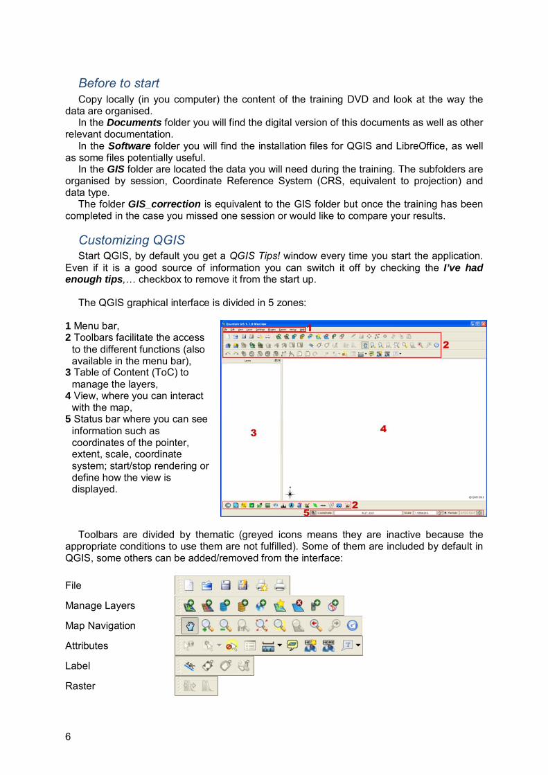
The Color Map function of mmqgis allows to apply a blend of 3 colours legend, and to fix manually the threshold values for rasters AND vectors.
Unfortunately the plugin does not automatically detect the minimum and maximum values to render, then you will have to get them yourself through the Metadata tab of the layer Properties. Try to generate a legend such at the one in the next figure.
To avoid displaying the ocean, set the No data
value to 0 in the Transparency tab of the layer Properties.
In the case the new display is not updated in the
View, you need to click on the Apply button, of the Colormap tab (layer Properties).
To complete this session we will consolidate the
QGIS project by reprojecting the only layer who displays through the ‘on the fly’ CRS transformation function: Right click on Administrative Units, Save as…, Save as: …\GIS\1_Introduction\JAD2001\Vector\SALB.shp,
CRS: JAD2001 / Jamaica Metric Grid, Click twice the OK button and replace the Administrative units layer by the new one.
Before to close this session let’s have a look at how QGIS store projects. In a text editor
(e.g. notepad) open the .qgs file you just created and look at the structure of the file in general and the way it store the data in particular.
The projects are stored using common XML format, absolute paths to the layers are stored with the datasource tag. It means several things: The layers are not included in the .qgs file, When you share a project you need to copy the .qgs file AND ALL the layers in the project
and store them in the same location in the host computer. In order to facilitate things, you can save QGIS projects with relative paths. This way the
project and the data can be moved to any location or any computer as long as the structure of all files remains the same. To do so: Close the notepad and open your project in QGIS, Settings > Project Properties, set the Save paths options (General tab) to relative, Close all windows, save and close again your project, Open the .qgs file in the notepad and check the difference in the datasource tags.
Unfortunately the option to use relative paths can not be set as a default parameter, then
it has to be changed every time you create a new project. A rescue solution in the case you receive one project with absolute paths who do not fit
your computer structure is in a text editor to replace automatically the wrong path by the appropriate one in the .qgs file (do not forget to save a copy before to do so).
13
Population distribution One basic data need when analysing physical exposure is to know precisely where the
population is located. Unfortunately, global population distribution model remains too coarse for an analysis at the scale of the RiVAMP project. Then we need to process a population distribution grid by combining the census data with the location of the buildings in the Area of Interest (AOI).
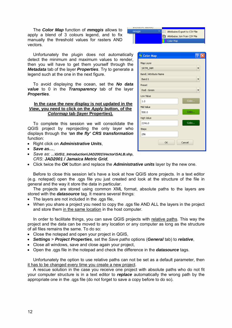
Load and explore the data Load all the .shp data in …\GIS\2_Population_Distribution\JAD2001\Vector. As the
Negril_Census_2001 layer does not contain any projection information QGIS should ask you to define one (JAD2001).
Now you should have in your project:
Negril_Census_2001: Unofficial population 2001 data,
Negril_random_buildings: Building locations randomly relocated within a 200 meter resolution grid for copyright reasons.
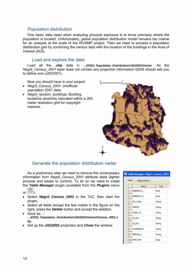
Generate the population distribution raster As a preliminary step we need to remove the unnecessary
information from Negril_Census_2001 attribute table (lighter process and easier to control). To do so we need to install the Table Manager plugin (available from the Plugins menu
or ): Select Negril_Census_2001 in the ToC, then start the
plugin, Select all fields except the few visible in the figure on the
right, press the Delete button and accept the deletion, Save as…:
…\GIS\2_Population_Distribution\JAD2001\Vector\Census_2001.shp,
Set up the JAD2001 projection and Close the window.

14
The new layer is automatically added to the project, then you can remove Negril_Census_2001 as it will no be needed anymore.
Now we will count the number of building in each census unit:
Vector > Analysis Tools > Points in polygon, If you have only the two necessary layers loaded, just define the Output Shapefile as
…\GIS\2_Population_Distribution\JAD2001\Vector\Census_2001_cnt.shp, OK > OK > Yes > JAD2001 > OK > Close (optionally you can remove Census_2001),
Do not worry about the warning message saying the CRS are different, it is simply
because JAD2001 projection is quite rare and QGIS attributes a custom CRS instead of an “official” one.
Open the Attribute table of the new layer and check the validity of the values (minimum,
maximum and visually) you just generated. Let’s calculate the average number of inhabitant per building and census unit:
Open Census_2001_cnt attribute table,
Switch to the Editing mode using button,
Start the Field calculator with the button, Create a New field: AVEINHAB, Decimal number, 5, 1, Apply the following formula: MAN_FEM / PNTCNT > OK,
Switch off the Editing mode ( ) > Save and close the attribute table. This time let’s have a deeper look at the
data we generated (in order to avoid surprises coming from erroneous values further in the process): Vector > Analysis Tools > Basic
statistics, Census_2001_cnt, AVEINHAB > OK,
Values vary between 0,6 and 15,0 with a mean around 3,8 and a standard deviation of 2,3. Without surprise the figure in the right shows that the beach has the lowest values when the populated places have the highest values (as the census data does not include tourists).

15
Now transfer the average number of people leaving in habitations to the building layer through a spatial link: Vector > Data Management Tools >
Join attributes by location >>, Add the layer to the display and optionally remove Negril_random_buildings. Using the Table Manager plugin, remove all fields except AVEINHAB then Rename the remaining field as HAB (otherwise the field name will become too long in the next join action) and Save.
We need now to create a vector grid of 50 meter resolution to aggregate the information
by “cell” (even if we are still in vector format): Vector > Research Tools > Vector grid,
Grid extent: Census_2001_cnt, Update extents from layer button, Round the X and Y values to 50 meter and set a 50 meter resolution (but this value can be increased if your computer is a little weak) Save the Output shapefile as …\GIS\2_Population_Distribution\JAD2001\Vector\VGrid_50m.shp, OK > Yes > Close.
Check visually the vector grid covers fully the Census layer. Finally let’s combine the virtual grid with
the number of inhabitant through a spatial link: Vector > Data Management Tools >
Join attributes by location >>,

16
The number of people leaving in each “cell” will be automatically stored in a field named SUMHAB.
As we are at the end of the process we need to estimate the error of our model, a simple
way to do it is simply to sum and compare the fields MAN_FEM and SUMHAB in the layers Census_2001_cnt and VGrid_50m_Hab respectively (Using Vector > Analysis Tools > Basic statistics). That makes an error of 33 inhabitants in a total of 40,215!
To conclude we will convert the virtual grid into a true raster but because the rasterization
function in QGIS will ask the number of columns and rows we need to calculate them before to start: Get the metadata of VGrid_50m_Hab and divide the difference of extensions by 50 meter
in X and Y (in my case X: (625400-605250)/50 = 403, Y: (694150-672200)/50 = 439
Raster > Rasterize (Vector to raster) >> Check the output raster overlays perfectly
with the vector as well as the higher and lower values seem logically located.
17
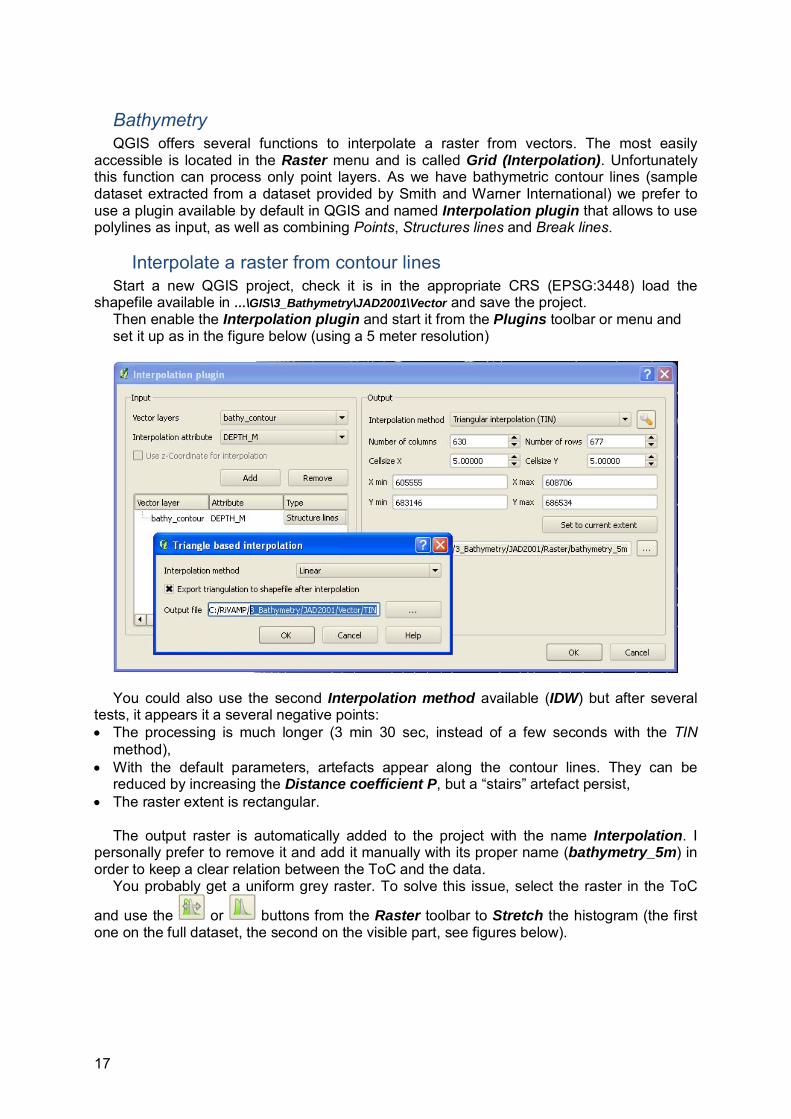
Bathymetry QGIS offers several functions to interpolate a raster from vectors. The most easily
accessible is located in the Raster menu and is called Grid (Interpolation). Unfortunately this function can process only point layers. As we have bathymetric contour lines (sample dataset extracted from a dataset provided by Smith and Warner International) we prefer to use a plugin available by default in QGIS and named Interpolation plugin that allows to use polylines as input, as well as combining Points, Structures lines and Break lines.
Interpolate a raster from contour lines Start a new QGIS project, check it is in the appropriate CRS (EPSG:3448) load the
shapefile available in …\GIS\3_Bathymetry\JAD2001\Vector and save the project. Then enable the Interpolation plugin and start it from the Plugins toolbar or menu and set it up as in the figure below (using a 5 meter resolution)
You could also use the second Interpolation method available (IDW) but after several
tests, it appears it a several negative points: The processing is much longer (3 min 30 sec, instead of a few seconds with the TIN
method), With the default parameters, artefacts appear along the contour lines. They can be
reduced by increasing the Distance coefficient P, but a “stairs” artefact persist, The raster extent is rectangular.
The output raster is automatically added to the project with the name Interpolation. I
personally prefer to remove it and add it manually with its proper name (bathymetry_5m) in order to keep a clear relation between the ToC and the data.
You probably get a uniform grey raster. To solve this issue, select the raster in the ToC
and use the or buttons from the Raster toolbar to Stretch the histogram (the first one on the full dataset, the second on the visible part, see figures below).

18
Full stretch Local strech
Optionally you can add the TIN shapefile to the project to visualize the way the TIN
algorithm works. Try to use the Interactive Identify plugin (the
plugin you should have installed during the
introduction session) by clicking the button and then clicking on the View.
You should get an error message. Close the Python error window and access the Interactive
identify configuration window through the button. By default this tool gives a lot of information and it seems some of them are bugged. I am personally just interested in getting the value of the selected layers in a given position, then I configure it like in the figure on the right. This way you should not get an error anymore.
Let’s imagine a partner ask you to provide you with a bathymetric data at 10 meter
resolution in a “rustic” format such has xyz: Raster > Translate (Convert format),
Output file: bathy_pts_10m.xyz, Outsize: 50% (this way the raster will be aggregated from 5 to 10 meter resolution)
By default the no data pixels have a value of -9999, then to correctly display this layer you have to set up the No data value to -9999 in the Transparency tab of the Properties of the layer.

19
Flooded area exposure The aim of this session is firstly to define the land areas potentially exposed to floods due
to tropical cyclones and secondly to estimates the population and assets that will be affected. To do so, we will first use an aggregated version (for copyright reason) of the Digital
Elevation Model (DEM) provided by Jamaican Government, and the maximum elevation of wave height calculated during the wave modelling for two return period (10 and 50 years). Then we will use the population distribution raster we created in a previous session, as well as an assets location layer provided by Jamaican Government.
Identify the flooded areas To delineate the flooded area we will reclassify the DEM on the base of the values in the
table below (corresponding to the maximum simulated wave height).
10 yrp 50 yrp
Beach 3.6 m 6.7 m
Cliff 7.5 m 8.0 m
Create a new project, add it the DEM (…\GIS\4_Flood_Exposure\JAD2001\Raster\DEM_12m.tif)
and save the project. As the elevation of the wave vary between the beach and cliff shoreline we need to create
a mask that will delineate both areas: Vector > Research Tools > Polygon from layer extent, Save the Output polygon shapefile as:
…\GIS\4_Flood_Exposure\JAD2001\Vector\tmpAOI.shp and add it to the project,
Zoom to the cliff area, create a new Polygon shapefile
(named tmpCliff) with the button,
Edit the layer ( ) and draw ( ) the cliff area according to the figure on the right (right click to close the polygon), stop editing and save,
Then Union the two vector layers (Vector > Geoprocessing Tools > Union), save the layer as tmpUnion, and add it to the project (optionally you can remove the two other vector layers),
Open the Attribute table, edit it, remove the record containing the little polygon outside the Area Of Interest (AOI),
With the Field calculator, create a new field (Cliff, Whole number, 2), set the value to 1 in the cliff area and to 0 in the remaining area, Save the changes and Close the attribute table.
20
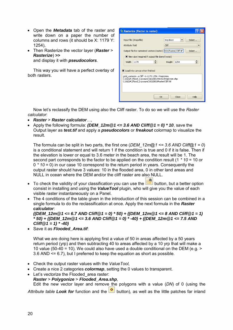
Open the Metadata tab of the raster and write down on a paper the number of columns and rows (it should be X: 1179 Y: 1254),
Then Rasterize the vector layer (Raster > Rasterize) >> and display it with pseudocolors. This way you will have a perfect overlay of
both rasters.
Now let’s reclassify the DEM using also the Cliff raster. To do so we will use the Raster
calculator: Raster > Raster calculator…, Apply the following formula: (DEM_12m@1 <= 3.6 AND Cliff@1 = 0) * 10, save the
Output layer as test.tif and apply a pseudocolors or freakout colormap to visualize the result.
The formula can be split in two parts, the first one (DEM_12m@1 <= 3.6 AND Cliff@1 = 0) is a conditional statement and will return 1 if the condition is true and 0 if it is false. Then if the elevation is lower or equal to 3.6 meter in the beach area, the result will be 1. The second part corresponds to the factor to be applied on the condition result (1 * 10 = 10 or 0 * 10 = 0) in our case 10 correspond to the return period in years. Consequently the output raster should have 3 values: 10 in the flooded area, 0 in other land areas and NULL in ocean where the DEM and/or the cliff raster are also NULL.
To check the validity of your classification you can use the button, but a better option consist in installing and using the ValueTool plugin, who will give you the value of each visible raster instantaneously on a Panel.
The 4 conditions of the table given in the introduction of this session can be combined in a single formula to do the reclassification at once. Apply the next formula in the Raster calculator: ((DEM_12m@1 <= 6.7 AND Cliff@1 = 0) * 50) + ((DEM_12m@1 <= 8 AND Cliff@1 = 1) * 50) + ((DEM_12m@1 <= 3.6 AND Cliff@1 = 0) * -40) + ((DEM_12m@1 <= 7.5 AND Cliff@1 = 1) * -40)
Save it as Flooded_Area.tif: What we are doing here is applying first a value of 50 in areas affected by a 50 years return period (yrp) and then subtracting 40 to areas affected by a 10 yrp that will make a 10 value (50-40 = 10). We could also have used a double conditional on the DEM (e.g. > 3.6 AND <= 6.7), but I preferred to keep the equation as short as possible.
Check the output raster values with the ValueTool, Create a nice 2 categories colormap, setting the 0 values to transparent. Let’s vectorize the Flooded_area raster:
Raster > Polygonize > Flooded_Area.shp, Edit the new vector layer and remove the polygons with a value (DN) of 0 (using the
Attribute table Look for function and the button), as well as the little patches far inland

21
that obviously will not be flooded (to make things easier you can install and use the selectplus plugin).
Compute the exposure Add to the project the assets and population layers that will be processed. The first one is
available at …\GIS\4_Flood_Exposure\JAD2001\Vector\assets_pts.shp. You processed the second one during the Population distribution session (Buildings_Hab.shp), you can use you own or a version clipped to the AOI (…\GIS\4_Flood_Exposure\JAD2001\Vector\Buildings_Hab_clip.shp).
Using the Attribute table Look for function select all polygons with a value of 10 in
Flooded_Area. Then clip the two point layers (Vector > Geoprocessing Tools > Clip) with the flooded
area (use all features for the 50 yrp, and only the selected features in Flooded_area for the 10 yrp). You will get 4 layers: flooded_assets_10yrp flooded_assets_50yrp flooded_population_10yrp flooded_population_50yrp
Assets exposure can be easily synthesized through a map such as on the right showing the number of assets exposed (use the Show feature count option of the context menu) and their location, but we still need to process a little bit the population exposure.
22
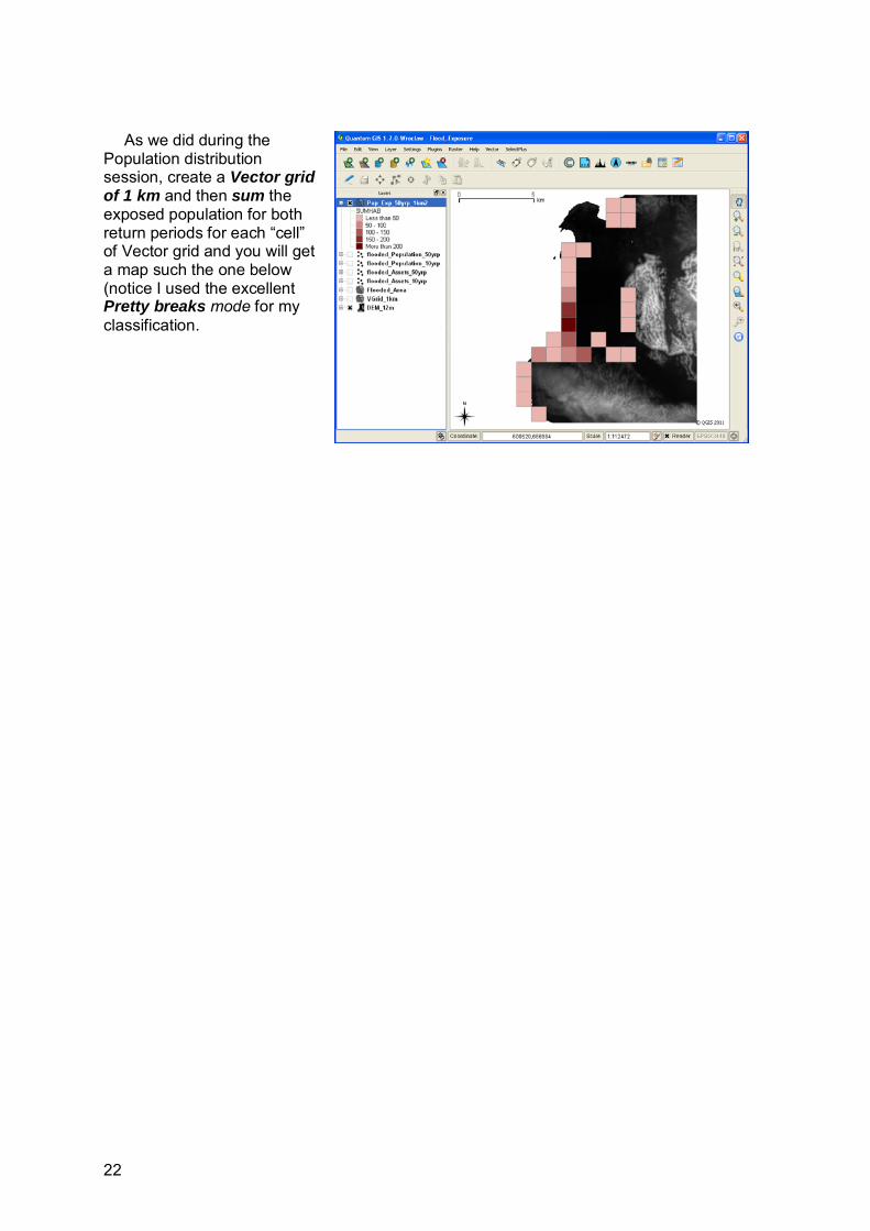
As we did during the
Population distribution session, create a Vector grid of 1 km and then sum the exposed population for both return periods for each “cell” of Vector grid and you will get a map such the one below (notice I used the excellent Pretty breaks mode for my classification.

23
Profile extraction The aim of this session is to draw profiles perpendicular to the shoreline and extract the environmental and bathymetric parameters that will be used during the Statistical analysis training.
Draw the profiles Create a new project, add it the beach profile layer
(…\GIS\5_Profile_Extraction\JAD2001\Vector\Beach_Profiles.shp) and save the project. To locate yourself add land_classif_negril.shp and bathy_4m.tif in the same folder. As
you will notice the style of the land classification layer is already defined as a .qml file with the same name exist, it is automatically used (notice the partial transparency of some categories).
The beach profiles have been acquired and kindly provided by Smith and Warner International (in fact the layer we are using only contains a sample of the full dataset). The eastern ends correspond to the inland limit of the beach, the western ends to the shoreline at the time of the profile acquisition.
First we need to extend the profile toward the ocean but it can not be done completely
within QGIS: Convert the beach profiles layer to points with the Extract nodes function of the Vector
menu > Beach_ends.shp, Then add the nodes coordinates to the attribute table with the Export/Add geometry
columns of the same menu > Beach_ends_xy.shp, Do not forget to save your project before to start a spreadsheet editor (in our case with
LibreOffice Calc (installation file available in the Software folder of the training DVD, you need to close QGIS during the installation)),
Within LibreOffice Calc open the attribute table of the last layer > …\GIS\5_Profile_Extraction\JAD2001\Vector\Beach_ends_xy.dbf, and save the table as Beach_ends_xy.ods
In order to facilitate the reading of the table Rename the 3 headers in row #1 to PROFILE_ID, XCOORD,YCOORD,
Each profile fit in two rows, in general the second one corresponds to the shoreline end, but we need to make sure of that. Write the following formula in cell D3 and copy it until the bottom of the dataset. =IF(A3=A2,IF(B2>B3,0,1),0) This formula will return a “1” in the case the X coordinate value of the second point of a profile is higher than the first one (meaning the ends are inversed), Check if you have any 1 value (in this case you should inverse the rows of a given profile, When it is done you can delete the D column,
Let’s use Pythagoras theorem to calculate the oceanic end for 3 kilometres (3000 metres) extension of each profile into the ocean, Add three headers in the column D, E and F (respectively Length, Xoc, Yoc, In cell E2 add the formula: =B3, In cell F2 add: =C3, In cell D3 add: =SQRT((B2-B3)^2+(C2-C3)^2), In cell E3 add: =B3-(3000*(B2-B3)/$D3), In cell F3 add: =C3-(3000*(C2-C3)/$D3),
24
Copy the 6 cells to the bottom of the dataset using the drag and drop functionality,
Copy the values (see figure on the right) of the all dataset into a new sheet and remove the column B, C and D, Finally save the file as usual, and save it again as .csv (only the active sheet will be saved), before to close LibreOffice.
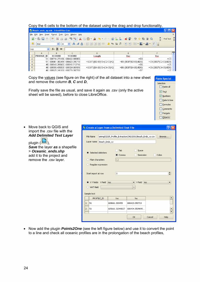
Move back to QGIS and
import the .csv file with the Add Delimited Text Layer
plugin ( ), Save the layer as a shapefile > Oceanic_ends.shp add it to the project and remove the .csv layer.
Now add the plugin Points2One (see the left figure below) and use it to convert the point
to a line and check all oceanic profiles are in the prolongation of the beach profiles,
25
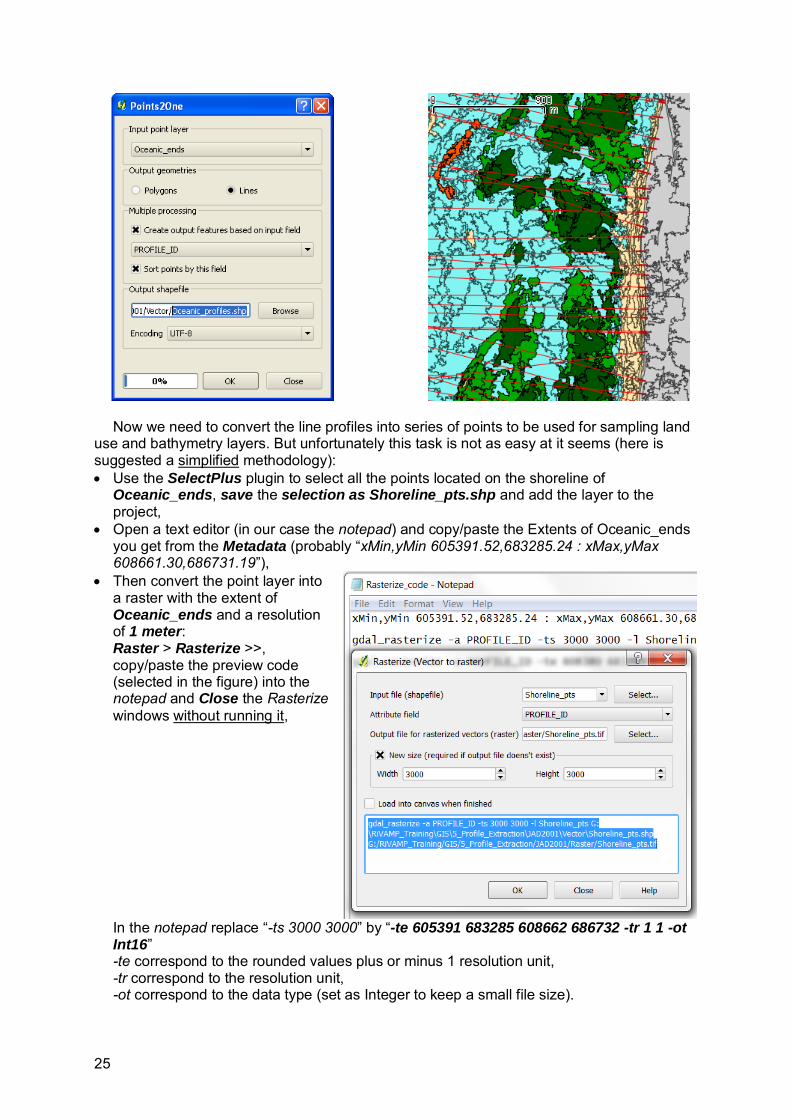
Now we need to convert the line profiles into series of points to be used for sampling land
use and bathymetry layers. But unfortunately this task is not as easy at it seems (here is suggested a simplified methodology): Use the SelectPlus plugin to select all the points located on the shoreline of
Oceanic_ends, save the selection as Shoreline_pts.shp and add the layer to the project,
Open a text editor (in our case the notepad) and copy/paste the Extents of Oceanic_ends you get from the Metadata (probably “xMin,yMin 605391.52,683285.24 : xMax,yMax 608661.30,686731.19”),
Then convert the point layer into a raster with the extent of Oceanic_ends and a resolution of 1 meter: Raster > Rasterize >>, copy/paste the preview code (selected in the figure) into the notepad and Close the Rasterize windows without running it,
In the notepad replace “-ts 3000 3000” by “-te 605391 683285 608662 686732 -tr 1 1 -ot Int16” -te correspond to the rounded values plus or minus 1 resolution unit, -tr correspond to the resolution unit, -ot correspond to the data type (set as Integer to keep a small file size).

26
From the start button start msys copy/paste (pressing the scroll button of your mouse) the modified code and press Enter (you might have to convert “\” into “/”),
We have to do that because by default the Rasterize function of QGIS does not allows the user to define the extent and resolution of the output raster, but these options exist in gdal. Close msys and the notepad and add the raster you just created to your QGIS project, check the raster covers totally the Oceanic_profiles layer, set the No data value to “0” in the Transparency tab),
Using this raster compute a distance raster with the Proximity function of the Raster
menu > dist_1m.tif, and add it to your project, As you can see this function covers the raster to process extent, this is the reason why we had to force this parameter by using msys in the previous step.
Convert the raster into a contour layer with 5 meter interval (to keep processing time short) and intersect it with the profiles: Raster > Contour >>,
Intersect the contour lines with the profiles to create the sampling points: Vector > Analysis Tools > Line intersections >>,
27
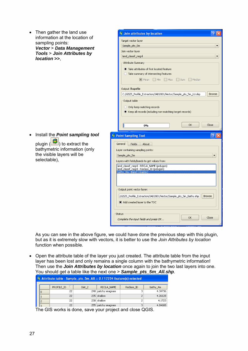
Then gather the land use information at the location of sampling points: Vector > Data Management Tools > Join Attributes by location >>,
Install the Point sampling tool
plugin ( ) to extract the bathymetric information (only the visible layers will be selectable),
As you can see in the above figure, we could have done the previous step with this plugin, but as it is extremely slow with vectors, it is better to use the Join Attributes by location function when possible.
Open the attribute table of the layer you just created. The attribute table from the input layer has been lost and only remains a single column with the bathymetric information! Then use the Join Attributes by location once again to join the two last layers into one. You should get a table like the next one > Sample_pts_5m_All.shp.
The GIS works is done, save your project and close QGIS.
28
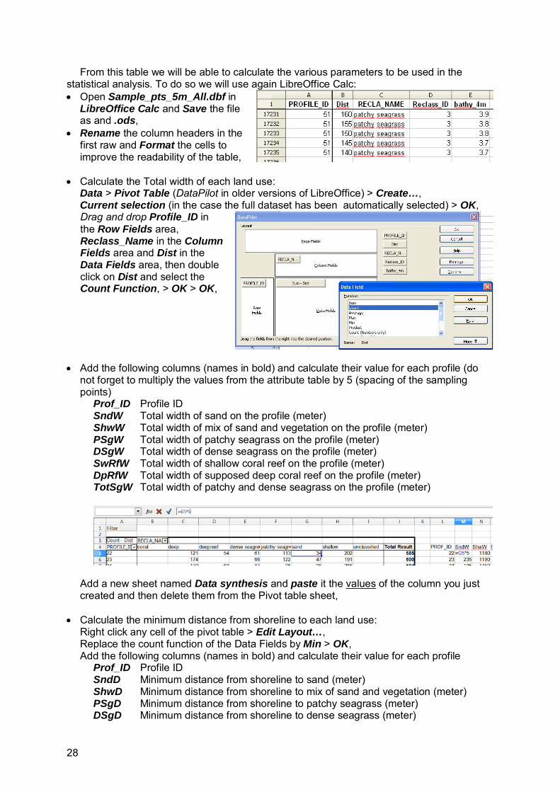
From this table we will be able to calculate the various parameters to be used in the statistical analysis. To do so we will use again LibreOffice Calc: Open Sample_pts_5m_All.dbf in
LibreOffice Calc and Save the file as and .ods,
Rename the column headers in the first raw and Format the cells to improve the readability of the table,
Calculate the Total width of each land use: Data > Pivot Table (DataPilot in older versions of LibreOffice) > Create…, Current selection (in the case the full dataset has been automatically selected) > OK, Drag and drop Profile_ID in the Row Fields area, Reclass_Name in the Column Fields area and Dist in the Data Fields area, then double click on Dist and select the Count Function, > OK > OK,
Add the following columns (names in bold) and calculate their value for each profile (do
not forget to multiply the values from the attribute table by 5 (spacing of the sampling points)
Prof_ID Profile ID SndW Total width of sand on the profile (meter) ShwW Total width of mix of sand and vegetation on the profile (meter) PSgW Total width of patchy seagrass on the profile (meter) DSgW Total width of dense seagrass on the profile (meter) SwRfW Total width of shallow coral reef on the profile (meter) DpRfW Total width of supposed deep coral reef on the profile (meter) TotSgW Total width of patchy and dense seagrass on the profile (meter)
Add a new sheet named Data synthesis and paste it the values of the column you just created and then delete them from the Pivot table sheet,
Calculate the minimum distance from shoreline to each land use: Right click any cell of the pivot table > Edit Layout…, Replace the count function of the Data Fields by Min > OK, Add the following columns (names in bold) and calculate their value for each profile
Prof_ID Profile ID SndD Minimum distance from shoreline to sand (meter) ShwD Minimum distance from shoreline to mix of sand and vegetation (meter) PSgD Minimum distance from shoreline to patchy seagrass (meter) DSgD Minimum distance from shoreline to dense seagrass (meter)

29
SwRfD Minimum distance from shoreline to shallow coral reef (meter) DpRfD Minimum distance from shoreline to supposed deep coral reef (meter) MinSgD Minimum distance from shoreline to patchy or dense seagrass (meter)
Paste the values of the column you just created in the Data synthesis sheet and then delete them from the Pivot table sheet (check the Profile_IDs coincide between the two tables), As the 0 values correspond to no data in these columns, replace 0 by 9999 to symbolize the difference.
Calculate the average depth in a given distance (within a 50 meter radius) from the shoreline: Copy the original sheet (containing the sampled data) to a new sheet named Bathymetry, Keep only the columns relative to the Profile_ID, Dist and the bathy_4m, Sort the table with the Dist column, In a new column named Dist2Shore, write down 500 in all rows with a Dist value between 450 and 550, do the same with Dist values of 1000, 1500, 2000, 2500, 3000 (keeping a +- 50 meter tolerance), Create a Pivot table (this time you will have to select the cells first) with Profile_ID, Dist2Shore and the Average of bathy_4m as Data Field, Copy the relevant values of the content table (without the empty columns and Total values) into the Data synthesis sheet and rename the columns into
Dpt500 Average depth (50 meter radius) around 500 m from shoreline (meter) Dpt1000 Average depth (50 meter radius) around 1000 m from shoreline (meter) Dpt1500 Average depth (50 meter radius) around 1500 m from shoreline (meter) Dpt2000 Average depth (50 meter radius) around 2000 m from shoreline (meter) Dpt2500 Average depth (50 meter radius) around 2500 m from shoreline (meter) Dpt3000 Average depth (50 meter radius) around 3000 m from shoreline (meter)
Keep 1 digit format and replace the empty cells by 9999.
Calculate the maximum distance from the shoreline to reach a given depth: Sort the table in Bathymetry sheet with the bathy_4m column, Add a new column named DepthCat and fill it with the rounded value of bathy_4m, Right click in any cell of the pivot table of the bathymetry sheet > Edit Layout… > More > extend the selection until the E column, then change the layout with Profile_ID, DepthCat and the Min of Dist, Copy the relevant values of the content table (without the Total values) into the Data synthesis sheet, remove the columns that are not 4, 5, 6, 7, 8, 9, 10, 12, 14, 16, 20 and rename the columns into
Prof4 Maximal distance to reach the 4 meter depth (meter) Prof5 Maximal distance to reach the 5 meter depth (meter) Prof6 Maximal distance to reach the 6 meter depth (meter) Prof7 Maximal distance to reach the 7 meter depth (meter) Prof8 Maximal distance to reach the 8 meter depth (meter) Prof9 Maximal distance to reach the 9 meter depth (meter) Prof10 Maximal distance to reach the 10 meter depth (meter) Prof12 Maximal distance to reach the 12 meter depth (meter) Prof14 Maximal distance to reach the 14 meter depth (meter) Prof16 Maximal distance to reach the 16 meter depth (meter) Prof20 Maximal distance to reach the 20 meter depth (meter)
That’s it you are now ready to perform the statistical analysis

30
Plugins selection GdalTools: Need to be upgraded at the time of writing this document AND enabled to access all functionalities of the Raster menu. Interactive identify: Query several layers at once with extended configuration settings. mmqgis: Various helpful GIS functions. Point sampling tool: Collect values from multiple layers (vector AND raster). Points2One: Create polygon or polyline from points. SelectPlus: Menu with selection options. Table manager: Manage attribute table structures Value tool: Instantaneous display of raster values.
References Quantum GIS website: http://qgis.org/ Python plugins repositories: http://www.qgis.org/wiki/Python_Plugin_Repositories GRASS GIS website: http://grass.fbk.eu/ GDAL: http://www.gdal.org/index.html LibreOffice: http://www.libreoffice.org/
Index Add delimited text layer 19 Basic statistics 10 Clip (vector) 17 Colormap 7 Contour (raster) 21 Export(Add geometry columns) 18 Extract nodes 18 Field calculator 10 GDAL 21 Interpolation plugin 13 Join attributes per location 11 Label 6 Line intersections 21 msys (GDAL) 21 No data (Transparency) 8 Pivot table 23 Plugins 3
Point sampling tool 22 Points in polygon 10 Points2One 19 Polygon from layer extent 15 Polygonize (Raster to vector) 16 (Layers) Properties 6 Raster calculator 16 Rasterize (Vector to raster) 12 (General) Settings 4 Show feature count 17 Stretch (histogram) 13 SVG 6 Translate (Convert format raster) 14 Union (vector) 15 Vector grid 11 Warp (Reproject raster) 7
31
RiVAMP statistical analysis Training
Some theory
Statistical concepts For readers who are not familiar with some of the statistical concepts used in this training,
here is a small summary. This section is adapted from the on-line help of StatSoft Electronic Statistics Textbooks (http://www.statsoft.com/textbook/statistics-glossary/).
This example was made for a research on links between deforestation and landslides in North Pakistan (see Peduzzi, P., Landslides and vegetation cover in the 2005 North Pakistan earthquake: a GIS and statistical quantitative approach, Nat. Hazards Earth Syst. Sci., 10, 623-640, 2010. http://www.nat-hazards-earth-syst-sci.net/10/623/2010/nhess-10-623-2010.html).
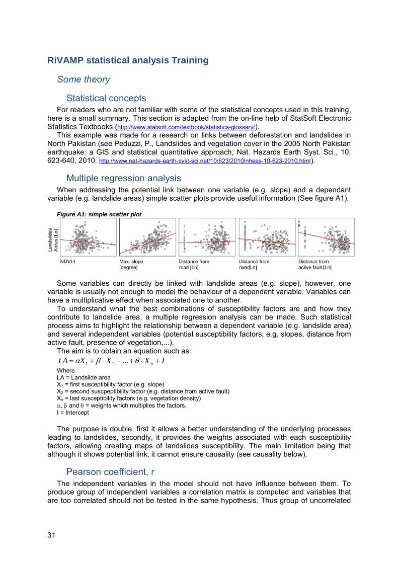
Multiple regression analysis When addressing the potential link between one variable (e.g. slope) and a dependant
variable (e.g. landslide areas) simple scatter plots provide useful information (See figure A1). Figure A1: simple scatter plot
Some variables can directly be linked with landslide areas (e.g. slope), however, one
variable is usually not enough to model the behaviour of a dependent variable. Variables can have a multiplicative effect when associated one to another.
To understand what the best combinations of susceptibility factors are and how they contribute to landslide area, a multiple regression analysis can be made. Such statistical process aims to highlight the relationship between a dependent variable (e.g. landslide area) and several independent variables (potential susceptibility factors, e.g. slopes, distance from active fault, presence of vegetation,...).
The aim is to obtain an equation such as: IXXXLA n ...21
Where LA = Landslide area X1 = first susceptibility factor (e.g. slope) X2 = second suscpeptibility factor (e.g. distance from active fault) Xn = last susceptibility factors (e.g. vegetation density) , and = weights which multiplies the factors. I = Intercept The purpose is double, first it allows a better understanding of the underlying processes
leading to landslides, secondly, it provides the weights associated with each susceptibility factors, allowing creating maps of landslides susceptibility. The main limitation being that although it shows potential link, it cannot ensure causality (see causality below).
Pearson coefficient, r The independent variables in the model should not have influence between them. To
produce group of independent variables a correlation matrix is computed and variables that are too correlated should not be tested in the same hypothesis. Thus group of uncorrelated

32
variables should be created (see appendix C). The r is the pearson coefficient (or correlation coefficient), it is computed as follows:
22 )()(
)()(
yyxx
yyxxr
where
x is the average for a observed dependant variable
y is the average for the modelled variable
In this study, two independent variables could be placed in the same group if |r| < 0.5.
R2 and Adjusted R2 R2 is the square of r, it provides an indication of the percentage of variance explained. Adjusted R2 is a modification of R2 that adjusts for the number of explanatory terms in a
model. Meaning that by adding more explanatory variables you might increase the R2, but it could also be by chance (over fitting models). The Adjusted R2 is particularly useful in the selection of potential susceptibility factors as it takes into account the number of explanatory variables and only increase if the added explanatory variable explains more than as a result of a coincidence.
1
1)1(1. 22
pn
nRRadj
Where n is the sample size, p is the number of independent variables in the model. In general terms, the more explanatory variables you have the less the R2, because by
introducing more independent variables, you increase the risk that the results is obtained by random. This is often called “overfitting”.
Normal distribution The variables should follow a normal distribution. This can be done by looking at
histograms and by applying some statistical normality tests (e.g. Normal expected frequencies, Kolmogorov-Smirnov & Lilliefors test for normality, Shapiro-Wilk’s W test.). If a variable do not follow a normal distribution, it needs to be transformed so that it does (e.g. computing the Ln, or using transformation formula). The figure below shows the distribution of landslide areas. Taking the Ln greatly improve the normality.
Figure A2: normality
Other functions can be used as specified in the article.

33
Correlation matrix A sound statistical multiple regression analysis do not include dependant variables which
are correlated between them. Compute the correlation between parameters and do not use two dependant variables which are correlated (e.g. r > 0.5).
This test can also be done after you find the model, however, this would help to reduce the amount of tests.
Outliers Outliers are cases that do not follow the general assumption. In the real environment, it is
difficult to take all the parameters reflecting the complexity of the situations. Some isolated cases, might have specific settings, and they don’t follow the general trends. These outliers are easy to identify as they are distant to the rest of the data. They should be identified and removed so that the general rule can be better identified. However, an analysis of these outliers should be performed to ensure that they don’t follow another rule. If this is the case, then the dataset might need to be split so that two (or more) models can be generated. For example, we differentiated landslides close to rivers and landslides away from rivers as it seems that these two groups follow different rules.
Causality Correlation between two variables (e.g. A & B) do not imply that variation of A is the origin
of the variation of B. If multiple regression can shows potential link, it cannot ensure causality. What we aim to do is to say that factor A (e.g. vegetation density) influence B (landslide
area). Now having a correlation between factors A & B can have several origins: A is indeed having an influence on B or B is influencing A or C is influencing A & B. The p-level provide good insight on the probability that the link is due to a coincidence.
However, addressing causality is always the main challenge (see discussion under “verification of causality”).
VARIABLES GEO_CLAS EPI7_LN DFPC2001 AFPC2001 DFPC1979 AFPC1979 D_DF_N FAU_E_LN RIV_E_LN ROAD_ELN AS_SLMAXGEO_CLAS 1EPI7_LN -0.61054494 1DFPC2001 0.030173617 0.064267123 1AFPC2001 0.151408464 -0.02053886 0.681399181 1DFPC1979 -0.157253167 0.150427599 0.511186591 0.407626633 1AFPC1979 -0.306262486 0.263142132 0.397172862 0.29143195 0.660796501 1D_DF_N -0.189837925 0.159892844 -0.054033713 0.009781408 0.557353372 0.379014984 1FAU_E_LN -0.574314739 0.509284177 -0.018360254 -0.059362492 0.132283622 0.194093629 0.126551334 1RIV_E_LN -0.027317046 -0.047358484 0.072998129 0.025901471 0.085597576 0.137044457 0.039028676 -0.109581934 1ROAD_ELN 0.245954832 -0.180364857 0.163845352 0.240070041 0.115202886 -0.03391631 -0.001611524 -0.191126149 0.006302733 1AS_SLMAX -0.083784927 0.069787184 0.01342266 -0.000396599 0.069191982 0.244110713 0.064153034 0.037619704 -0.030041463 -0.035268997 1LN_AREA 0.322441637 -0.329124405 0.022722721 0.069425912 -0.110669497 0.004488764 -0.077697417 -0.357883868 -0.217723769 0.084802057 0.546452847
34
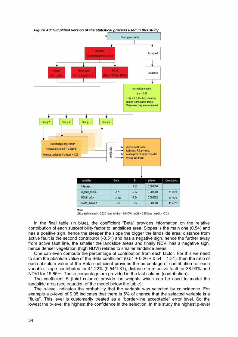
Figure A3: Simplified version of the statistical process used in this study
In the final table (in blue), the coefficient “Beta” provides information on the relative
contribution of each susceptibility factor to landslides area. Slopes is the main one (0.54) and has a positive sign, hence the steeper the slope the bigger the landslide area; distance from active fault is the second contributor (-0.51) and has a negative sign, hence the further away from active fault line, the smaller the landslide areas and finally NDVI has a negative sign, hence denser vegetation (high NDVI) relates to smaller landslide areas.
One can even compute the percentage of contribution from each factor. For this we need to sum the absolute value of the Beta coefficient (0.51 + 0.26 + 0.54 = 1.31), then the ratio of each absolute value of the Beta coefficient provides the percentage of contribution for each variable: slope contributes for 41.22% (0.54/1.31), distance from active fault for 38.93% and NDVI for 19.85%. These percentage are provided in the last column (contribution).
The coefficient B (third column) provide the weights which can be used to model the landslide area (see equation of the model below the table).
The p-level indicates the probability that the variable was selected by coincidence. For example a p-level of 0.05 indicates that there is 5% of chance that the selected variable is a “fluke”. This level is customarily treated as a “border-line acceptable” error level. So the lowest the p-level the highest the confidence in the selection. In this study the highest p-level

35
was 0.0018, meaning all the selected variables have less than 0.18% chance of being selected by coincidence.
What is a good model? Models are not the reality, they try to approximate it based on a simplification. A good
model is a model which : 1) Explains a significant part of the differences observed (look at R2 values, they represent
the percentage of variance explained). 2) If you have a good R2, this is not enough, the distribution should be along a line.
Observe the distribution between observed versus modelled, ideally, your points on the scatterplot should be representing a line.
3) The number of independant variables is not too high (e.g. between 2 and 4), if you have too many independant variables, your model may be data driven. To test this, look at the adj. R2 as well as test your model on one part of your data (e.g. 2/3) and keep the other part (1/3) for validating your model. You can also do this in an iterative way (e.g. bootstrap process).
4) Look at the p-value of your independant variables, they should be < 0.05. 5) Test if the independant variables are not auto-correlated, run a correlation matrix
between the independant variables and look if all the r are < 0.5. 6) Make sure you have enough records, the more you have the higher the confidence in
your model.
36
In brief The aim of this training is to introduce you to statistical analysis in the context of a study
such as RiVAMP. The open source statistical analysis software TANAGRA will be used. The training documentation has been prepared under a Windows XP environment, but is
easily reproducible in any other OS after a few adjustments.
Typographic convention In a general manner the text you have to focus because it figures in the applications has
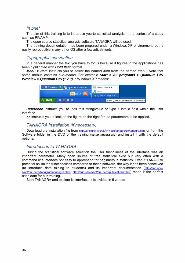
been highlighted with Bold Italic format. Menu > Item Instructs you to select the named item from the named menu. Note that
some menus contains sub-menus. For example Start > All programs > Quantum GIS Wroclaw > Quantum GIS (1.7.0) in Windows XP means:
Reference instructs you to look this string/value or type it into a field within the user
interface. >> instructs you to look on the figure on the right for the parameters to be applied.
TANAGRA installation (if necessary) Download the installation file from http://eric.univ-lyon2.fr/~ricco/tanagra/en/tanagra.html or from the
Software folder in the DVD of the training (setup.tanagra.exe) and install it with the default options.
Introduction to TANAGRA During the statistical software selection the user friendliness of the interface was an
important parameter. Many open source of free statistical exist but very often with a command line interface not easy to apprehend for beginners in statistics. Even if TANAGRA potential as limited functionalities compared to these software, the way it has been conceived (to introduce data mining to students) and its important documentation (http://eric.univ-lyon2.fr/~ricco/tanagra/en/tanagra.html, http://eric.univ-lyon2.fr/~ricco/publications.html) made it the perfect candidate for our training.
Start TANAGRA and explore its interface. It is divided in 5 zones:

37
1 Menu bar, 2 Toolbar to manage the project
and define variables, 3 Components (or operators)
library divided into sub-categories,
4 Data mining diagram, 5 Results view of each
components.
Data preparation and importation in TANAGRA Because TANAGRA do not work well with records containing nodata, some work on raw
data is necessary: Open the file …\Statistic\RiVAMP_Negril_Erosion.xls in LibreOffice Calc (a description of the
different variables is available in the ReadMe sheet). Copy the Data sheet in first position and rename it
Seagrass_small_sample. As the aim of RiVAMP project in Negril is to quantify the amount of
shoreline protection provided by bathymetry, seagrass meadows and shallow coral reef, we need to split the dataset in two. In our case we will analyse the protection provided by seagrass then we will remove the record containing shallow coral reef. Sort the copied table by SwRfW and remove the records with values higher than 0 (61 records are remaining). Remove the columns related to shallow coral reef (SwRfW and SwRfD). Sort back the table by Prof_ID, find empty cells and remove the related records (47 records are remaining).
Save the xls file and save again the first table as Text CSV with Tab field delimiter > seagrass_small_sample.csv.
Rename the file from .csv to .txt. Then import the data in TANAGRA:
Start TANAGRA, File > New… Fill the windows as in the
Figure >>

38
Check that 40 attributes and 47 examples (records) have been imported. In the case you have missed any nodata value, an error message will figure in front of the related attribute in the Dataset description table.
Explore the dataset Visualize the table by drag and dropping the Data visualization / View dataset
component in Dataset (in the diagram). And double click it to display it. Add also some graph functionalities by adding the Scatterplot with label component. Take some notes with the information you can see and could be helpful during the manual
linear regression. Test the normality of the dependant variable (in our case ErTot
(Maximum erosion 1968-2008 based on 2006 shoreline (meter)): In the diagram select Dataset and click on the button,
Add ErTot to the Input list > OK. Drag Statistics / More univariate cont stat to Define status 1,
Have a look at the Histogram and decide if fits a Gaussian distribution: Is the Average more or less equivalent to the Median? Is the MAD/STDDEV ratio near 0.7979? Are the Skewness and Kurtosis values near 0?
In the case of a perfect Gaussian distribution the average and the median values are the
same, the Skewness and Kurtosis values equal 0, and the ratio MAD/STDDEV = 0.7979. But all these parameters are only informative and do not imply at 100% the distribution is
not normal. We can go further with a normality test:
Drag Statistics / Normality Test stat to Define status 1. The normality test includes 4 tests, in the case the normality is verified the cells appears in
green, if they are not they display in red. In case of doubt they appear in grey. In our case, no test is either positive or negative then we can continue the analysis without
transforming the dataset before to start again the process. Let’s now visualize the correlation between the variables:
Add a new Define status to the Dataset with ErTot as Target variable and all other variables as Input.
Drag Statistics / Linear correlation stat to Define status 2, Parameters… > check the sort results checkbox, select the ¦r¦-value as well as the Target and Input options. The maximum r2 is quite low (0.24) and show no high correlation between the dependant
variable and one of the independent variables. Without surprise Er08 shows of the best correlation with ErTot as they are both representative of the erosion rate. TotSgW, PSgW, ShwW and a few bathymetric parameters appears as potentially interesting.

39
Clarify ideas through automatic regression Let’s TANAGRA suggest a reasonable regression model:
Drag Regression / Forward entry regression stat to Define status 2,
R2 remains similar to the values
obtained from one by one linear correlation. The 2 suggested variables are significant (the deeper the red, the better) even if Prof5 as limited significance.
Let’s increase the number of variable in the model by increasing significantly the Sig. level
to 0.3 in the Parameters. TotSgW remains the main parameters followed by Prof6, then Dpt2000, Prof10, PSgW,
Prof 5 and Irbn5y. Following this first analysis we can conclude, TotSgW is THE main explicative variable,
with one bathymetric variable to define. Then we can increase the dataset with a limited number of variables and start again the analysis with a more complete dataset.
Save your project and close TANAGRA before to do so.

40
Increase the dataset Open again the file RiVAMP_Negril_Erosion.xls and create a new table with a maximum of
records without nodata (by limiting the number of variables) to be imported in TANAGRA > Seagrass_large_sample.tdm.
I personally removed all the minimum distance as well as the Dpt3000 variables who seems to be not significant and reduced the dataset, that give me 33 attributes and 61 examples.
Repeat the data exploration and automatic regression
This time the normality test give worse values but as they are not 100% sure let’s continue the analysis.
The automatic regression confirms the strong significance of TotSgW, followed by bathymetric indicators, and potentially Iribarren number.
Precise manually the model through manual iterations Add a new Define status with ErTot as Target, TotSgW and Dpt2000 as Input and add it
the Regression / Multiple linear regression component > R2 = 0.177 and Dpt2000 is not significant.

41
Try to find the best model by testing each bathymetric variable. When it is done try to add a third variable (not representative of the bathymetry) and see if it increase R2 and is significant.
Prof5 seems to give the best model (significant with a R2 = 0.315), but Prof6, Dpt1000
and Dpt1500 also seems interesting. The best third variable seems to be one of the Irribaren numbers, as they all increase R2
to 0.341, but remains no significant. The combination of PSgW, DsgW and Prof5 is also one potential model (R2 = 0.319
(0.349 with one Irribaren variable (not significant)).
Improve the model by removing outliers Let’s find and remove outliers of a model with TotSgW, Prof5 and Irbn5y:
Set the appropriate Parameters of Define status 3, Add a Regression / Outlier detection component to Multiple linear regression 1.
Move to the Values tab and list the potential outliers (based on 6 test, they are highlighted in orange).
Add also a Regression / DfBetas component (it will highlight the records that have the bigger influence on the model). Move to the DfBetas tab and list the potential outliers (highlighted in orange). Create a synthesis table such as
Outlier detection
0 1 2 3 4
DfBetas 0 33, 34 60, 61 391 25, 35 4 38
2 28 44 The record 44 is showed 4 times as an outlier and has an important impact on the model.
The records 38 is tested 4 times as an outlier with a smaller impact on the model. The records 25, 28 and 35 seems to have a greta impact but are not detected as outliers.
Add a Data visualization / Scatterplot with label component to Multiple linear
regression 1 and graph ErTot vs Pred_lmreg_1 and/or Err_Pred_lmreg1. Records 38 and 39 have a ErTot values of 0, that could correspond
to artificial beach nourishment. On the other side record 44 could correspond to an exceptional erosion rate. Then in a first time we will remove the records 38 and 39 from the analysis.
As we cannot remove records from the dataset simply by using their ID, we have to find
the Prof_ID of the 2 records to remove with View dataset 1> Prof_ID = 44 and 45. Then we can create 2 conditions filters: Add an Instance selection / Rule-based selection component to Define status 3,
Parameters: Add the 2 following conditions Prof_ID<>44 And Prof_ID<>45 (we could have instead used the less generic single condition (ErTot<>0).
Move Multiple linear regression 1 into Rule-based selection1. Notice how the Examples values decreased from 61 to 59. R2 increased to 0.443 and
Irbn5y became more significant.

42
Play a while with the model by removing other outliers and replacing variables in order to attempt to improve the model.
The model TotSgW, Prof5 and Irbn5y (or any other Iribarren number) gives the best
results (R2 = 0.443, with Irbn5y partially significant). The model PSgW, DSgW, Prof5 and Irbn5y gives also good results (R2 = 0.445), but
DSgW is not significant and Irbn5y is only partially significant, then this model will not be continued.
43
Database of Beach Retreat Projections and Beach Retreat Estimators
Introduction
The Database of Beach Retreat Projections and the Beach Retreat Estimator comprise a
tool that can estimate the range of beach retreat for different morphologically beaches, under
different scenarios of long-term and short-term sea level rise and different conditions/forcing
(in terms of sedimentology and hydrodynamics). The incorporated database has resulted
though the construction/application of ensembles (a short-term and a long-term ensemble) of
different 1-D analytical and numerical morphodynamic models of varied complexity. It must
be noted that this tool does not intend to replace detailed studies, which are based upon the
2-D/3-D morphodynamic modles calibrated/validated through the collection of
comprehensive sets of field observations (see McLeod et al., 2010 for a review); rather, it
aims to provide an easily deployed methodology that can provide a rapid first assessment of
beach erosion/inundation risk under sea level rise.
Beach retreat morphodynamic models
Beaches are among the most morphologically dynamic environments, being controlled by
complex process-response mechanisms that operate in several temporal and spatial scales
(Van Rijn, 2003). Beach erosion can be differentiated into: (i) long-term erosion, i.e.
irreversible retreat of the shoreline position, due to sea level rise and/or negative coastal
sedimentary budgets (Nicholls et al., 2007) that force either landward migration of the
beaches or drowning; and (ii) short-term erosion, caused by storms and storm surges, which
may not necessarily result in permanent shoreline retreats, but may create large-scale
devastation (Niedoroda et al., 2009).
Sea level rise can have significant impacts on beach geomorhology, as beaches will be
forced to retreat (Fig. 1). The extent and rate of the beach retreat depend on several
parameters, e.g. the beach slope, the type/supply of beach sediments and the hydrodynamic
conditions (Dean, 2002).
44
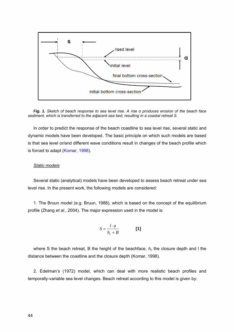
Fig. 1. Sketch of beach response to sea level rise. A rise α produces erosion of the beach face
sediment, which is transferred to the adjacent sea bed, resulting in a coastal retreat S.
In order to predict the response of the beach coastline to sea level rise, several static and
dynamic models have been developed. The basic principle on which such models are based
is that sea level or/and different wave conditions result in changes of the beach profile which
is forced to adapt (Komar, 1998).
Static models
Several static (analytical) models have been developed to assess beach retreat under sea
level rise. In the present work, the following models are considered:
1. The Bruun model (e.g. Bruun, 1988), which is based on the concept of the equilibrium
profile (Zhang et al., 2004). The major expression used in the model is:
Bh
alS
c
[1]
where S the beach retreat, B the height of the beachface, hc the closure depth and l the
distance between the coastline and the closure depth (Komar, 1998).
2. Edelman’s (1972) model, which can deal with more realistic beach profiles and
temporally-variable sea level changes. Beach retreat according to this model is given by:
45
)(ln)(
taBh
BhwtS
b
obb
[2]
where the Bo is the initial height of the beachface, wb, is the surf zone width and hb is the
water depth at wave breaking.
3. The Dean (1991) model, which was developed for the diagnosis/prediction of storm-
driven beach retreat, is also based on the equilibrium profile concept, with the beach retreat
controlled by the water depth at wave breaking, the height of breaking waves Hb, the surf
zone width, according to the following expression:
b
bb hB
wHaS
068.0 [3]
Dynamic models
The dynamic (numerical) models used in the present tool are:
4. The SBEACH model (Larson and Κraus, 1989), which is a ‘bottom-up’ morphodynamic
model, consisting of combined hydrodynamic, sediment transport and morphological
development modules. The hydrodynamic module contains detailed descriptions of the wave
transformation, with its basic expression being:
FsFF EE
h
k
dx
dE [4]
where k is an empirical wave decay coefficient, EF is the wave energy flux and EFs is the
stable wave energy flux. The sediment transport is controlled by the wave energy flux and
the beach slope according to the equations below:
)(dx
dhDDq eq
, dx
dhDD eq
[5]
0q , dx
dhDD eq
[6]
where K is an empirical transport rate coefficient, D is the wave energy dissipation per unit
volume, Deq is equilibrium energy dissipation per unit volume and ε is a transport rate

46
coefficient for the slope-dependent term. Finally, the sediment continuity equation on which
the morphological development model is based upon, is addressed by finite differences and
a ‘stair – step’ beach profile discretisation.
5. The model based on the Leont’yev (1996) algorithm uses the energetics approach
(Battjes and Janssen, 1978), with the wave energy balance in the cross-shore direction
controlled by the wave propagation angle , the group velocity cg the wave energy E and its
dissipation due to breaking D:
D
x
cE g
cos
[7]
Sediment transport rates are predicted separately for the surf and swash zones. The
transport rate qW due to wave/current interaction is determined following Leont’yev (1996):
1
23 ~3cos~tan2
x
d
U
WBFUuufq
d
ssdW
bW
[8]
where fW is the bed friction coefficient for wave orbital velocities u (Nielsen, 1992), Ud is
the wave undertow velocity, Ws is the sediment fall velocity and εs is the efficiency factor of
suspended load transport. F and B express power ‘expenditure’ due to bed friction (F) and
excess turbulence at the bottom layer (Roelvink and Stive, 1989). On the surf zone, run up
sediment transport is estimated using Leont’yev (1996):
tantan2 2/31 eqR gRcq
[9]
where c1 is a dimensionless proportionality coefficient and tanβe is the equilibrium beach
slope (Bascom, 1964). For the swash zone, run up transport rate is given by:
MRMR
MRR xxx
xx
xxqq
2/3
/1
/1
[10]
where xR, xM are the lower and upper limit of the swash zone. The run-up induced
transport rate qR decays away from the swash zone towards the outer boundary of the surf
zone according to:

47
oRRR Hxxcqq /exp 3 Rxx [11]
The suspended and bed load transport rates are assumed to decay linearly to zero from
the breaking point to the beach border. Finally, the beach profile evolution is estimated by
solving the sediment continuity equation through a forward finite differences scheme.
Introduction to Matlab GUI
A graphical user interface (GUI) provides the user with a familiar environment. This
environment contains familiar to the user push-buttons, toggle-buttons, lists, menus, text
boxes etc, so that he or she can concentrate on using the application rather than on the
mechanics involved. The 3 principal elements required to create a MATLAB Graphical User
Interface are:
1. Components. Each item of a MATLAB GUI (push-buttons, labels, edit boxes, etc) is a
graphical component. The types of components include graphical controls (push-buttons, edit
boxes, lists, sliders, etc.), static elements (frames and text strings), menus, and axes.
Graphical controls and static elements are created by the function uicontrol, and menus are
created by the functions uimenu and uicontextmenu. Axes, which are used to display
graphical data, are created by the function axes.
2 Figures. The components of a GUI must be arranged within a figure, which is a window
on the computer screen. In the past, figures have been created automatically whenever there
were data to be plotted. However, empty figures can be created through he function figure
and can be used to hold any combination of components.
3 Callbacks. Finally, there must be some way to perform an action if a user clicks a mouse
on a button or types information on a keyboard. A mouse click or a key press is an event,
and the MATLAB program must respond to each event if the program is to perform its
function. For example, if a user clicks on a button, that event must cause the MATLAB code
that implements the button function to be executed. The code that is executed in response to
an event is known as a call back. There must be a callback to implement the function of each
graphical component on the GUI. MATLAB GUIs are created using a tool called guide, the
GUI Development Environment. This tool allows a programmer to layout the GUI, selecting
and aligning the GUI components to be placed within it.

48
Once the components are in place, the programmer can edit their properties: name,
colour, size, font, text to display etc. In addition, the programmer may want to modify the Tag
parameters of the components. The Tag parameter is basically the variable name of a
component, and it is used as identifier in the programming code. When the Guide saves the
GUI, it creates a working program including skeleton functions (as m-file) that the
programmer can modify to implement the behaviour of the GUI. The m-file is where the
programmer attaches the appropriate code to the callback of each component. So a Matlab
GUI consists of (i) a figure which is the platform that the programmer has created and (ii) an
m-file created by Matlab guide and modified by the programmer.
Database of Beach Retreat Projections
Introduction
The models that were used to create this database are: 3 analytical (Edelman, Bruun,
Dean) (Edelman, 1972; Bruun, 1988; Dean, 1991) and 2 numerical models (SBEACH and
Leont’yev) (Larson and Kraus, 1989; Leont’yev, 1996). The models Leont’yev, SBEACH and
Edelman can estimate (mainly) short-term changes of beaches and the models Bruun and
Dean long-term changes. All models were applied for the case of beaches (low coasts
consisted of unconsolidated sediments) using linear profiles with slopes of 1/10, 1/15, 1/20,
1/25 and 1/30. Experiments were carried out using varying wave conditions, i.e. wave
heights (H) of 0.5, 1, 1.5, 2, 3, 4, 5 and 6 m and periods (T) 3- 12 s and 7 different sediment
grain sizes (d50 of 0.2, 0.33, 0.50, 0.80, 1, 2 and 5 mm). For all cases (totally 465), 14 sea
level rise scenarios (0.038, 0.05, 0.10, 0.15, 0.22, 0.30, 0.40, 0.50, 0.75, 1, 1.25, 1.50, 2 and
3 m) were tested.
In order for this volume of data to be manageable, a simplified platform was created using
the Matlab Guide. The users of this platform can search in the database for the
environmental conditions (beach slope, wave height, wave period, sediment size) of their
interest. They can use specific conditions (viz. one value for each parameter) and obtain (if
these conditions are found in the database) the beach retreat (for small spatial scale e.g. one
beach) given by the five models (Leont’yev, SBEACH, Edelman, Bruun and Dean) for 14 sea
level scenarios (0.038, 0.05, 0.10, 0.15, 0.22, 0.30, 0.40, 0.50, 0.75, 1, 1.25, 1.50, 2 and 3 m)
and the polynomial equation that describes the relation between sea level rise and beach
retreat. Users can select all, or some of these models to create an ensemble and then they
can obtain the mean values (by selected models) of beach retreat and the polynomial
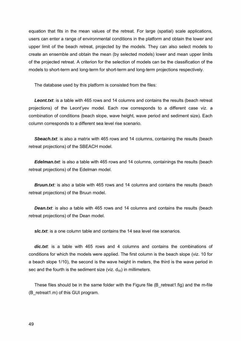
49
equation that fits in the mean values of the retreat. For large (spatial) scale applications,
users can enter a range of environmental conditions in the platform and obtain the lower and
upper limit of the beach retreat, projected by the models. They can also select models to
create an ensemble and obtain the mean (by selected models) lower and mean upper limits
of the projected retreat. A criterion for the selection of models can be the classification of the
models to short-term and long-term for short-term and long-term projections respectively.
The database used by this platform is consisted from the files:
Leont.txt: is a table with 465 rows and 14 columns and contains the results (beach retreat
projections) of the Leont’yev model. Each row corresponds to a different case viz. a
combination of conditions (beach slope, wave height, wave period and sediment size). Each
column corresponds to a different sea level rise scenario.
Sbeach.txt: is also a matrix with 465 rows and 14 columns, containing the results (beach
retreat projections) of the SBEACH model.
Edelman.txt: is also a table with 465 rows and 14 columns, containings the results (beach
retreat projections) of the Edelman model.
Bruun.txt: is also a table with 465 rows and 14 columns and contains the results (beach
retreat projections) of the Bruun model.
Dean.txt: is also a table with 465 rows and 14 columns and contains the results (beach
retreat projections) of the Dean model.
slc.txt: is a one column table and contains the 14 sea level rise scenarios.
dic.txt: is a table with 465 rows and 4 columns and contains the combinations of
conditions for which the models were applied. The first column is the beach slope (viz. 10 for
a beach slope 1/10), the second is the wave height in meters, the third is the wave period in
sec and the fourth is the sediment size (viz. d50) in millimeters.
These files should be in the same folder with the Figure file (B_retreat1.fig) and the m-file
(B_retreat1.m) of this GUI program.

50
How to use this program
First, open up MATLAB. Go to the command window and type in guide, or use the icon
(GUIDE) below of the main menu. You should see the following screen appear (Figure
2), choose Open Existing GUI and then choose or browse the file you want to open e.g. for
this GUI the file B_retreat1.
Figure 2. Open files window.
You should now see the following screen (or something similar depending on what version
of MATLAB you are using):
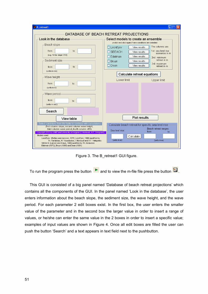
51
Figure 3. The B_retreat1 GUI figure.
To run the program press the button and to view the m-file file press the button .
This GUI is consisted of a big panel named ‘Database of beach retreat projections’ which
contains all the components of the GUI. In the panel named ‘Look in the database’, the user
enters information about the beach slope, the sediment size, the wave height, and the wave
period. For each parameter 2 edit boxes exist. In the first box, the user enters the smaller
value of the parameter and in the second box the larger value in order to insert a range of
values, or he/she can enter the same value in the 2 boxes in order to insert a specific value;
examples of input values are shown in Figure 4. Once all edit boxes are filled the user can
push the button ‘Search’ and a text appears in text field next to the pushbutton.
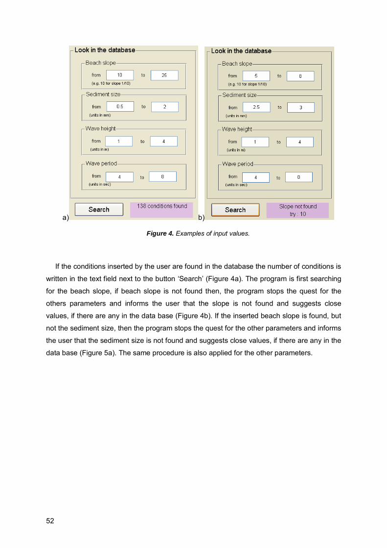
52
a) b)
Figure 4. Examples of input values.
If the conditions inserted by the user are found in the database the number of conditions is
written in the text field next to the button ‘Search’ (Figure 4a). The program is first searching
for the beach slope, if beach slope is not found then, the program stops the quest for the
others parameters and informs the user that the slope is not found and suggests close
values, if there are any in the data base (Figure 4b). If the inserted beach slope is found, but
not the sediment size, then the program stops the quest for the other parameters and informs
the user that the sediment size is not found and suggests close values, if there are any in the
data base (Figure 5a). The same procedure is also applied for the other parameters.

53
a) b)
Figure 5. Examples of input values not found.
Once the desired conditions are found, the user can use the button ‘View table’, which
prompts a list box to appear (Figure 6) with all the condition combinations found in the
database, enabling the user to view the results of his/her quest and make a new selection
from the list. Now that the environmental conditions are determined, the user can select
models to create an ensemble, by clicking in the corresponding checkboxes (Figure 7a). The
user has the option to view the lower and upper limit of beach retreat estimations made by
each model individually by pushing the button ‘View results’ next to the model (the checkbox
of the model should be clicked on) (Figure 7b). When the ‘View results’ button is pressed a
message box opens with a table consisted by 3 columns. The first column is the sea level
rise scenarios (in m), the second is the lower limit of beach retreat estimations (in m) made
by the model and the third column is the upper limit. If new conditions are selected, the
checkboxes should be un-clicked and clicked again, otherwise zero values appears in the
table in the message box.

54
Figure 6. The list box of the environmental conditions, 1st column: beach slope (m), 2nd column: wave height (m), 3rd column: wave period (sec), 4th column: sediment size (mm).
a) b)
Figure 7. a) An example of model selection. b) An example of message box with the results of Leont’yev model.
Once the models that comprise the ensemble are selected, the user can use the button
‘Calculate retreat equations’; then the polynomial equations describing the mean lower and
mean upper limits of beach retreat estimations appear in the text fields below the texts

55
‘Lower limit’ and ‘Upper limit’, respectively (see e.g. Figure 8). These equations have the
form: s = p1a2 +p2a +p3, where s: is the beach retreat, p1, p2 and p3: are the polynomial
coefficients and a: is the sea level rise. The value of R2 is also given in the text field.
Figure 8. An example of the resulted equations.
With the press of the pushbutton ‘Plot results’ the polynomials equations of the lower and
upper limit of all selected model are calculated and plotted together with the mean (non-
weighed) limits (see e.g. Figure 9).
Figure 9. An example of a plotting result. From the resulting equations, the range of beach retreat due to a sea level rise can be
calculated. This program gives the user the option to calculate the range of retreat only with

56
a click on the pushbutton ‘Calculate’ inside the panel ‘Calculate the retreat for a specific sea
level rise’. An example is given in Figure 10.
Figure 10. An example of beach retreat range calculation for a specific sea level rise scenario.
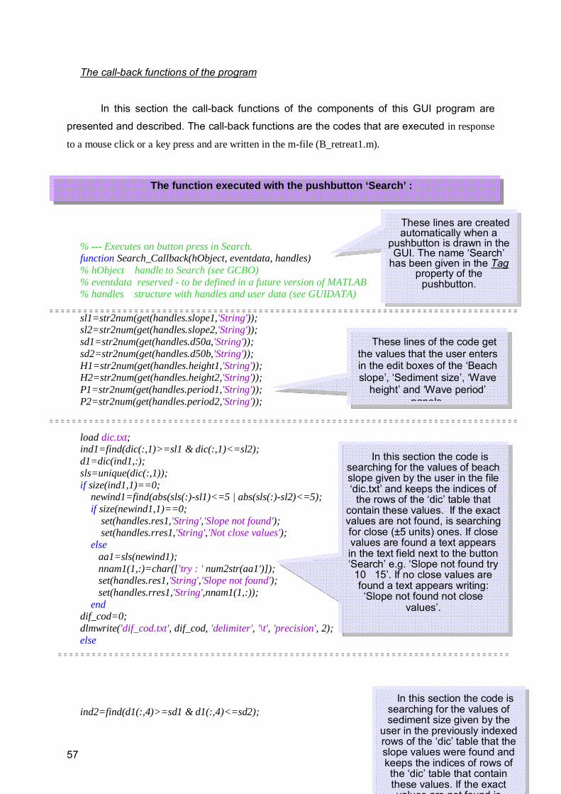
57
The call-back functions of the program
In this section the call-back functions of the components of this GUI program are
presented and described. The call-back functions are the codes that are executed in response
to a mouse click or a key press and are written in the m-file (B_retreat1.m).
% --- Executes on button press in Search. function Search_Callback(hObject, eventdata, handles) % hObject handle to Search (see GCBO) % eventdata reserved - to be defined in a future version of MATLAB % handles structure with handles and user data (see GUIDATA) sl1=str2num(get(handles.slope1,'String')); sl2=str2num(get(handles.slope2,'String')); sd1=str2num(get(handles.d50a,'String')); sd2=str2num(get(handles.d50b,'String')); H1=str2num(get(handles.height1,'String')); H2=str2num(get(handles.height2,'String')); P1=str2num(get(handles.period1,'String')); P2=str2num(get(handles.period2,'String')); load dic.txt; ind1=find(dic(:,1)>=sl1 & dic(:,1)<=sl2); d1=dic(ind1,:); sls=unique(dic(:,1)); if size(ind1,1)==0; newind1=find(abs(sls(:)-sl1)<=5 | abs(sls(:)-sl2)<=5); if size(newind1,1)==0; set(handles.res1,'String','Slope not found'); set(handles.rres1,'String','Not close values'); else aa1=sls(newind1); nnam1(1,:)=char(['try : ' num2str(aa1')]); set(handles.res1,'String','Slope not found'); set(handles.rres1,'String',nnam1(1,:)); end dif_cod=0; dlmwrite('dif_cod.txt', dif_cod, 'delimiter', '\t', 'precision', 2); else ind2=find(d1(:,4)>=sd1 & d1(:,4)<=sd2);
These lines are created automatically when a
pushbutton is drawn in the GUI. The name ‘Search’
has been given in the Tag property of the
pushbutton.
These lines of the code get the values that the user enters in the edit boxes of the ‘Beach slope’, ‘Sediment size’, ‘Wave
height’ and ‘Wave period’ panels
In this section the code is searching for the values of beach slope given by the user in the file ‘dic.txt’ and keeps the indices of
the rows of the ‘dic’ table that contain these values. If the exact values are not found, is searching for close (±5 units) ones. If close values are found a text appears in the text field next to the button ‘Search’ e.g. ‘Slope not found try
10 15’. If no close values are found a text appears writing: ‘Slope not found not close
values’.
In this section the code is searching for the values of sediment size given by the
user in the previously indexed rows of the ‘dic’ table that the slope values were found and keeps the indices of rows of the ‘dic’ table that contain these values. If the exact values are not found is
The function executed with the pushbutton ‘Search’ :

58
d2=d1(ind2,:); d50s=unique(d1(:,4)); if size(ind2,1)==0; newind2=find(abs(d50s(:)-sd1)<=1 | abs(d50s(:)-sd2)<=1); if size(newind2,1)==0; set(handles.res1,'String','Sediment size not found'); set(handles.rres1,'String','No close values'); else aa2=d50s(newind2); nnam2(1,:)=char(['try : ' num2str(aa2')]); set(handles.res1,'String','Sediment size not found'); set(handles.rres1,'String',nnam2(1,:)); end dif_cod=0; dlmwrite('dif_cod.txt', dif_cod, 'delimiter', '\t', 'precision', 2); else Hs=unique(d2(:,2)); ind3=find(d2(:,2)>=H1 & d2(:,2)<=H2); d3=d2(ind3,:); if size(ind3,1)==0; newind3=find(abs(Hs(:)-H1)<=1 | abs(Hs(:)-H2)<=1); if size(newind3,1)==0; set(handles.res1,'String','Wave height not found'); set(handles.rres1,'String','No close values'); else aa3=Hs(newind3); nnam3(1,:)=char(['try : ' num2str(aa3')]); set(handles.res1,'String','Wave height not found'); set(handles.rres1,'String',nnam3(1,:)); end dif_cod=0; dlmwrite('dif_cod.txt', dif_cod, 'delimiter', '\t', 'precision', 2); else
This section of the code is searching for the values of
wave height given by the user in the previously indexed rows
of the ‘dic’ table that the sediment sizes values were
found and keeps the indices of rows of the ‘dic’ table that
contain these values. If the exact values are not found is searching for close (±1 units)
ones. If close values are found a text appears in the text field next to the button ‘Search’ e.g.
‘Wave height not found try 1 2’. If no close values are found a text appears writing ‘Wave height not found not close
values’.

59
ind4=find(d3(:,3)>=P1 & d3(:,3)<=P2); Ts=unique(d3(:,3)); if size(ind4,1)==0; dif_cod=0; dlmwrite('dif_cod.txt', dif_cod, 'delimiter', '\t', 'precision', 2); newind4=find(abs(Ts(:)-P1)<=1 | abs(Ts(:)-P2)<=1); if size(newind4,1)==0; set(handles.res1,'String','Wave period not found'); set(handles.rres1,'String','No close values'); else aa4=Ts(newind4); nnam4(1,:)=char(['try : ' num2str(aa4')]); set(handles.res1,'String','Wave period not found'); set(handles.rres1,'String',nnam4(1,:)); end else k=size(ind4,1); dif_cod=d3(ind4,:); dlmwrite('dif_cod.txt', dif_cod, 'delimiter', '\t', 'precision', 2); nam(1,:)=char([num2str(k) ' conditions found']); set(handles.res1,'String',nam(1,:)); set(handles.rres1,'String',' '); end end end end
% --- Executes on button press in table. function table_Callback(hObject, eventdata, handles) % hObject handle to table (see GCBO) % eventdata reserved - to be defined in a future version of MATLAB % handles structure with handles and user data (see GUIDATA)
This section of the code is searching for the values of
wave period given by the user in the previously indexed rows of the ‘dic’ table that the wave periods values were found and keeps the indices of rows of the
‘dic’ table that contain these values. If the exact values are
not found is searching for close (±1 units) ones. If close values are found a text appears in the
text field next to the button ‘Search’ e.g. ‘Wave period not
found try 1 2’. If no close values are found a text appears writing ‘Wave period not found
not close values’.
If all values are found the code creates and
saves (as txt file) a new table named dif_cod with
the combinations of conditions that fulfil the
user’s request. The number of conditions
found appears as a text in the text field next to the
button ‘Search’.
Opens a list box with the conditions found in the database according with the criteria given by the user and saves the new selection of conditions made by the user in
a txt file named ‘Selection’. It also creates and saves 2 zero table (L_limit and U_limit) in which the limits of beach retreat estimations will be saved with the press of another
component.
Lines automatically
created with the creation of the
pushbutton ‘View table’.
The function executed with the pushbutton ‘View table’:

60
load dif_cod.txt; L_limit=zeros(5,14); U_limit=zeros(5,14); dlmwrite('L_limit.txt', L_limit, 'delimiter', '\t', 'precision', 6); dlmwrite('U_limit.txt', U_limit, 'delimiter', '\t', 'precision', 6); s=num2str(dif_cod); [Selection,ok]=listdlg('ListString',s,'name','conditions','ListSize',[200 300]); dlmwrite('Selection.txt', Selection, 'delimiter', '\t');
% --- Executes on button press in leo. function leo_Callback(hObject, eventdata, handles) % hObject handle to leo (see GCBO) % eventdata reserved - to be defined in a future version of MATLAB % handles structure with handles and user data (see GUIDATA) % Hint: get(hObject,'Value') returns toggle state of leo checkboxStatus = get(handles.leo,'Value'); load dif_cod.txt; load Selection.txt; dcod=dif_cod(Selection,:); load dic.txt; for i=1:size(dcod,1); ind4(i)=find(dic(:,1)==dcod(i,1) & dic(:,2)==dcod(i,2) & dic(:,3)==dcod(i,3) & dic(:,4)==dcod(i,4)); end load Leont.txt; load L_limit.txt; load U_limit.txt; if checkboxStatus==1; if size(ind4,2)==1; L_limit(1,:)=Leont(ind4,:); U_limit(1,:)=Leont(ind4,:); else L_limit(1,:)=min(Leont(ind4,:)); U_limit(1,:)=max(Leont(ind4,:)); end else
Lines automatically
created with the creation of the
checkbox ‘Leontyev’
If check box is clicked on the lower
and upper limit of the beach retreat estimations made by Leont’yev model are calculated and saved in the first
row of L_limit and U_limit tables respectively. Each row of these tables corresponds to a different model and each column to a different sea level
rise scenario. If check box is not clicked zero values are given in the
Leont’yev corresponding row (1st row) of the L_limit and U_limit tables.
Finds the indices of
the selected conditions, inside the dic table and loads the table with the
results of Leont’yev model.
The call-back function executed when the checkbox e.g. ‘Leontyev’ is clicked/unclicked:
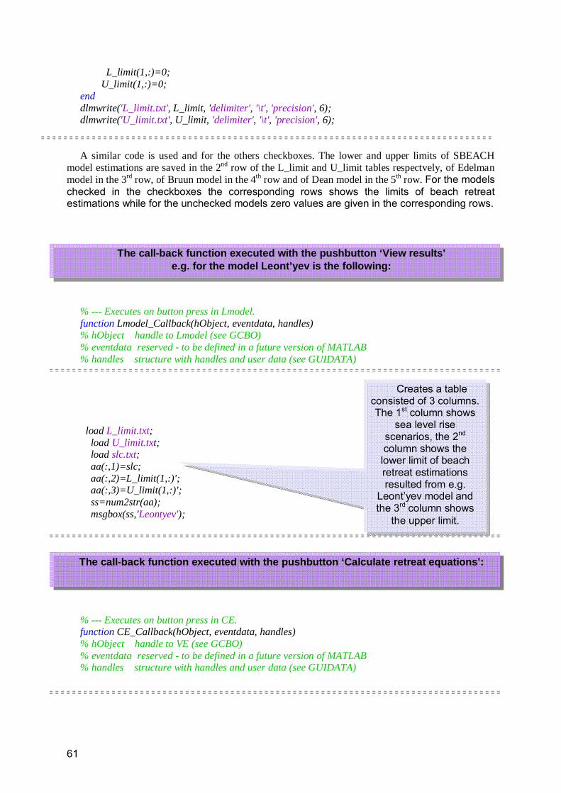
61
L_limit(1,:)=0; U_limit(1,:)=0; end dlmwrite('L_limit.txt', L_limit, 'delimiter', '\t', 'precision', 6); dlmwrite('U_limit.txt', U_limit, 'delimiter', '\t', 'precision', 6); A similar code is used and for the others checkboxes. The lower and upper limits of SBEACH
model estimations are saved in the 2nd row of the L_limit and U_limit tables respectvely, of Edelman model in the 3rd row, of Bruun model in the 4th row and of Dean model in the 5th row. For the models checked in the checkboxes the corresponding rows shows the limits of beach retreat estimations while for the unchecked models zero values are given in the corresponding rows.
% --- Executes on button press in Lmodel. function Lmodel_Callback(hObject, eventdata, handles) % hObject handle to Lmodel (see GCBO) % eventdata reserved - to be defined in a future version of MATLAB % handles structure with handles and user data (see GUIDATA) load L_limit.txt; load U_limit.txt; load slc.txt; aa(:,1)=slc; aa(:,2)=L_limit(1,:)'; aa(:,3)=U_limit(1,:)'; ss=num2str(aa); msgbox(ss,'Leontyev');
% --- Executes on button press in CE. function CE_Callback(hObject, eventdata, handles) % hObject handle to VE (see GCBO) % eventdata reserved - to be defined in a future version of MATLAB % handles structure with handles and user data (see GUIDATA)
The call-back function executed with the pushbutton ‘View results’ e.g. for the model Leont’yev is the following:
Creates a table consisted of 3 columns. The 1st column shows
sea level rise scenarios, the 2nd column shows the lower limit of beach retreat estimations resulted from e.g.
Leont’yev model and the 3rd column shows
the upper limit.
The call-back function executed with the pushbutton ‘Calculate retreat equations’:
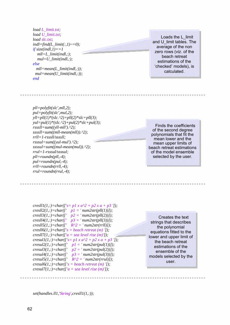
62
load L_limit.txt; load U_limit.txt; load slc.txt; indl=find(L_limit(:,1)~=0); if size(indl,1)==1 mll=L_limit(indl,:); mul=U_limit(indl,:); else mll=mean(L_limit(indl,:)); mul=mean(U_limit(indl,:)); end pll=polyfit(slc',mll,2); pul=polyfit(slc',mul,2); yll=pll(1)*(slc.^2)+pll(2)*slc+pll(3); yul=pul(1)*(slc.^2)+pul(2)*slc+pul(3); rsssll=sum((yll-mll').^2); ssssll=sum((mll-mean(mll)).^2); rrll=1-rsssll/ssssll; rsssul=sum((yul-mul').^2); ssssul=sum((mul-mean(mul)).^2); rrul=1-rsssul/ssssul; pll=roundn(pll,-4); pul=roundn(pul,-4); rrll=roundn(rrll,-4); rrul=roundn(rrul,-4); cresll1(1,:)=char(['s= p1 x a^2 + p2 x a + p3 ']); cresll2(1,:)=char([' p1 = ' num2str(pll(1))]); cresll3(1,:)=char([' p2 = ' num2str(pll(2))]); cresll4(1,:)=char([' p3 = ' num2str(pll(3))]); cresll5(1,:)=char([' R^2 = ' num2str(rrll)]); cresll6(1,:)=char(['s = beach retreat (m) ']); cresll7(1,:)=char(['a = sea level rise (m)']); cresul1(1,:)=char(['s= p1 x a^2 + p2 x a + p3 ']); cresul2(1,:)=char([' p1 = ' num2str(pul(1))]); cresul3(1,:)=char([' p2 = ' num2str(pul(2))]); cresul4(1,:)=char([' p3 = ' num2str(pul(3))]); cresul5(1,:)=char([' R^2 = ' num2str(rrul)]); cresul6(1,:)=char(['s = beach retreat (m) ']); cresul7(1,:)=char(['a = sea level rise (m)']); set(handles.ll1,'String',cresll1(1,:));
Loads the L_limit and U_limit tables. The
average of the non zero rows (viz. of the
beach retreat estimations of the
‘checked’ models), is calculated.
Finds the coefficients
of the second degree polynomials that fit the
mean lower and the mean upper limits of
beach retreat estimations of the model ensemble selected by the user.
Creates the text strings that describes
the polynomial equations fitted to the
lower and upper limit of the beach retreat estimations of the ensemble of the
models selected by the user.

63
set(handles.ll2,'String',cresll2(1,:)); set(handles.ll3,'String',cresll3(1,:)); set(handles.ll4,'String',cresll4(1,:)); set(handles.ll5,'String',cresll5(1,:)); set(handles.ll6,'String',cresll6(1,:)); set(handles.ll7,'String',cresll7(1,:)); set(handles.ul1,'String',cresul1(:,:)); set(handles.ul2,'String',cresul2(:,:)); set(handles.ul3,'String',cresul3(:,:)); set(handles.ul4,'String',cresul4(:,:)); set(handles.ul5,'String',cresul5(:,:)); set(handles.ul6,'String',cresul6(:,:)); set(handles.ul7,'String',cresul7(:,:));
% --- Executes on button press in plresults. function plresults_Callback(hObject, eventdata, handles) % hObject handle to plresults (see GCBO) % eventdata reserved - to be defined in a future version of MATLAB % handles structure with handles and user data (see GUIDATA) load L_limit.txt; load U_limit.txt; load slc.txt; indl=find(L_limit(:,1)~=0); if size(indl,1)==1 mll=L_limit(indl,:); mul=U_limit(indl,:); else mll=mean(L_limit(indl,:)); mul=mean(U_limit(indl,:)); end for i=1:size(indl,1); ppl(i,:)=polyfit(slc',L_limit(indl(i),:),2); yyl(i,:)=ppl(i,1)*(slc.^2)+ppl(i,2)*slc+ppl(i,3); ppu(i,:)=polyfit(slc',U_limit(indl(i),:),2); yyu(i,:)=ppu(i,1)*(slc.^2)+ppu(i,2)*slc+ppu(i,3); end pll=polyfit(slc',mll,2); pul=polyfit(slc',mul,2); yll=pll(1)*(slc.^2)+pll(2)*slc+pll(3); yul=pul(1)*(slc.^2)+pul(2)*slc+pul(3); yym=[flipud(yll);0;yul];
Displays the text strings created at the previous step in the
fields under the texts ‘Lower limit’ and ‘Upper
limit’.
The function executed with the pushbutton ‘Plot results’:
Finds the
coefficients of the second degree
polynomials that fit the beach retreat lower
and upper limit of the models selected by the
user.

64
tit(1,:)=char(['Leontyev']); tit(2,:)=char(['SBEACH ']); tit(3,:)=char(['Edelman ']); tit(4,:)=char(['Bruun ']); tit(5,:)=char(['Dean ']); tit(6,:)=char(['Mean ']); indnl=[indl;6]; xx1=[flipud(slc);0;slc]; colo=['r','k','b',']; typ=['-',':','-']; figure for i=1:size(indl,1); yy1(:,i)=[flipud(yyl(i,:)');0;yyu(i,:)']; pl=plot(xx1,yy1(:,i),typ(i)); set(pl,'color',colo(i)); hold on; end if size(indl,1)==1; hold off indnl=indl; else h=plot(xx1,yym,'--'); set(h,'color',[0.6 0.2 0],'linewidth',2); indnl=[indl;6]; end set(gca,'fontsize',15); xlabel('Sea level rise (m)','fontsize',22); ylabel('Beach retreat (m)','fontsize',22); legend(tit(indnl,:),'location','northwest'); axis tight; grid on;
% --- Executes on button press in CALCretreat. function CALCretreat_Callback(hObject, eventdata, handles) % hObject handle to CALCretreat (see GCBO) % eventdata reserved - to be defined in a future version of MATLAB % handles structure with handles and user data (see GUIDATA) slr=str2num(get(handles.SLRscenario,'String')); load L_limit.txt; load U_limit.txt; load slc.txt; indl=find(L_limit(:,1)~=0);
Plots the polynomials found for the selected models
together with the polynomials of the
means of these models
The function that is executed with the press of pushbutton ‘Calculate’:
Calculates the range of retreat for a specific sea
level rise scenario given by the user, in the edit box with
the Tag name ‘SLRscenario’ below the
text ‘Sea level rise:’ using the polynomial equations that describe the mean
l d th
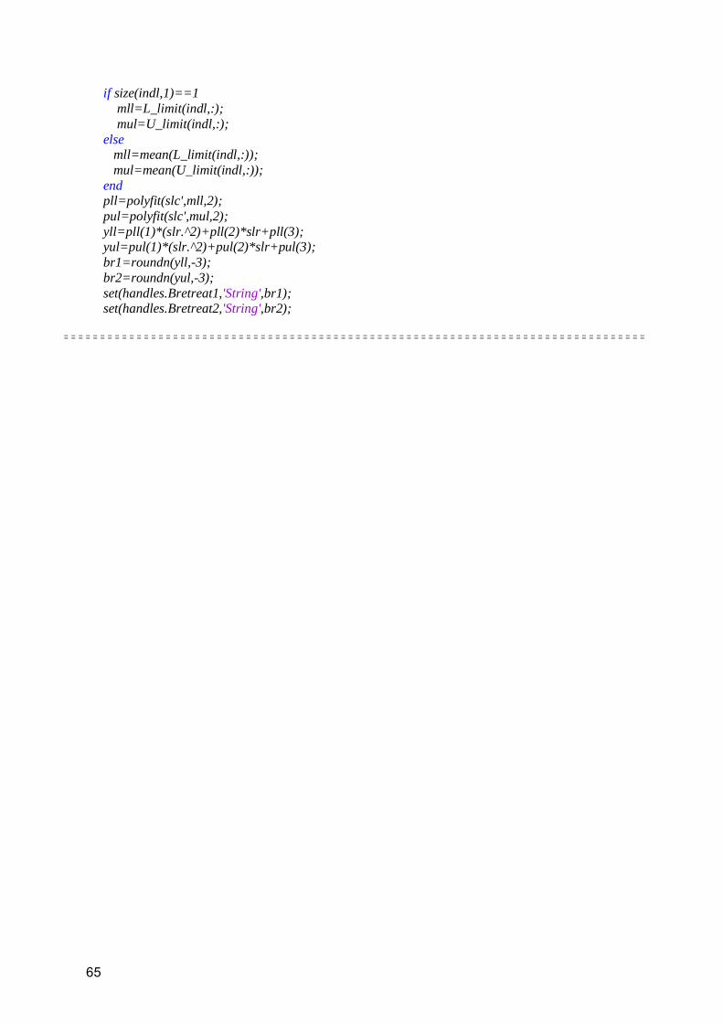
65
if size(indl,1)==1 mll=L_limit(indl,:); mul=U_limit(indl,:); else mll=mean(L_limit(indl,:)); mul=mean(U_limit(indl,:)); end pll=polyfit(slc',mll,2); pul=polyfit(slc',mul,2); yll=pll(1)*(slr.^2)+pll(2)*slr+pll(3); yul=pul(1)*(slr.^2)+pul(2)*slr+pul(3); br1=roundn(yll,-3); br2=roundn(yul,-3); set(handles.Bretreat1,'String',br1); set(handles.Bretreat2,'String',br2);

66
Beach Retreat Estimator Introduction The users of this GUI can estimate beach retreat according to static modles (Edelman’ s,
Bruun’s and Dean’s) for particular environmental conditions (beach slope, wave height, wave
period, sediment size) and sea level rise scenarios of their interest. The users can select all
or some of these models to create an ensemble and then they can obtain the mean values
(by selected models) of beach retreat and the polynomial equation that fits in the mean
values of the retreat. This GUI is consisted of the figure file (B_retreat2.fig) and the m-file
(B_retreat2.m).
How to use the program
Open up MATLAB. Use the icon (GUIDE) below of the main menu and open the file
B_retreat2. You should now see the screen shown in Figure 11. To run the program press
the button and to view the m-file file press the button .
In the panel named ‘Insert data’, the user enters information on beach slope, wave height
and wave period. He can also insert sea level rise scenarios pushing the button ‘Insert sea
level rise scenarios’. Then an input dialog box appears with default values been already
inserted which the user can use, or he/she can erase them and enter new values. The input
dialog box with default values is shown in Figure 12.
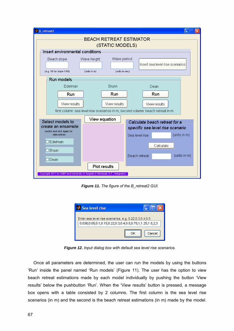
67
Figure 11. The figure of the B_retreat2 GUI.
Figure 12. Input dialog box with default sea level rise scenarios. Once all parameters are determined, the user can run the models by using the buttons
‘Run’ inside the panel named ‘Run models’ (Figure 11). The user has the option to view
beach retreat estimations made by each model individually by pushing the button ‘View
results’ below the pushbutton ‘Run’. When the ‘View results’ button is pressed, a message
box opens with a table consisted by 2 columns. The first column is the sea level rise
scenarios (in m) and the second is the beach retreat estimations (in m) made by the model.

68
An example of this message box is shown in Figure 13. The user can select models to create
an ensemble, by clicking in the corresponding checkboxes (Figure 14).
Figure 13. An example of message box with results of the Edelman model. Once the models comprising the ensemble are selected, the user use the button ‘View
equation’; then, a polynomial equation describing beach retreat estimations appears in the
text fields below the button. An example is shown in Figure 14. This equation have the form:
s = p1a2 +p2a +p3, where s: is the beach retreat, p1, p2 and p3: are the polynomial coefficients
and a: is the sea level rise. The value of R2 is also given in the text field.
Figure 14. An example of the resulted equation.
With the press of the pushbutton ‘Plot results’, the polynomial equations of all selected
models are calculated and plotted together with the polynomial equation that fits in the mean
values of beach retreat. An example of a plot result is depicted in Figure 15.
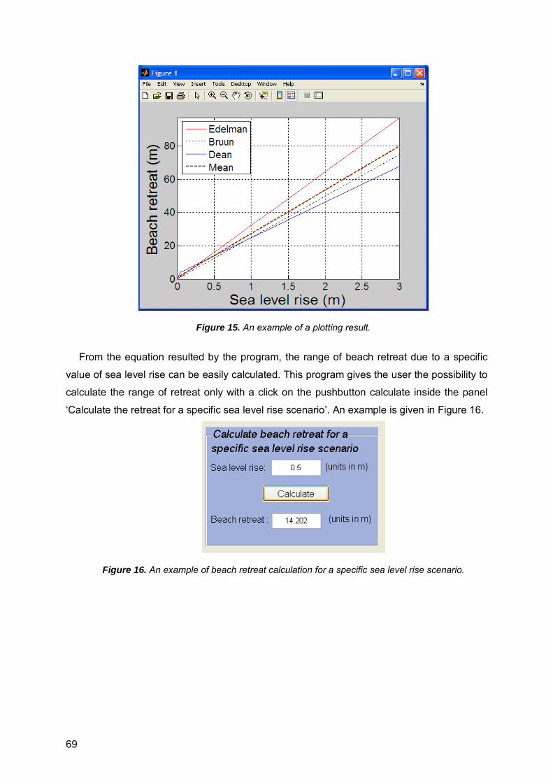
69
Figure 15. An example of a plotting result.
From the equation resulted by the program, the range of beach retreat due to a specific
value of sea level rise can be easily calculated. This program gives the user the possibility to
calculate the range of retreat only with a click on the pushbutton calculate inside the panel
‘Calculate the retreat for a specific sea level rise scenario’. An example is given in Figure 16.
Figure 16. An example of beach retreat calculation for a specific sea level rise scenario.
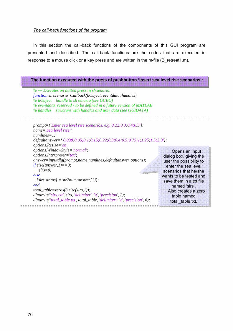
70
The call-back functions of the program
In this section the call-back functions of the components of this GUI program are
presented and described. The call-back functions are the codes that are executed in
response to a mouse click or a key press and are written in the m-file (B_retreat1.m).
% --- Executes on button press in slrsenario. function slrscenario_Callback(hObject, eventdata, handles) % hObject handle to slrsenario (see GCBO) % eventdata reserved - to be defined in a future version of MATLAB % handles structure with handles and user data (see GUIDATA) prompt={'Enter sea level rise scenarios, e.g. 0.22;0.3;0.4;0.5'}; name='Sea level rise'; numlines=1; defaultanswer={'0.038;0.05;0.1;0.15;0.22;0.3;0.4;0.5;0.75;1;1.25;1.5;2;3'}; options.Resize='on'; options.WindowStyle='normal'; options.Interpreter='tex'; answer=inputdlg(prompt,name,numlines,defaultanswer,options); if size(answer,1)==0; slrs=0; else [slrs status] = str2num(answer{1}); end total_table=zeros(3,size(slrs,1)); dlmwrite('slrs.txt', slrs, 'delimiter', '\t', 'precision', 2); dlmwrite('total_table.txt', total_table, 'delimiter', '\t', 'precision', 6);
Opens an input dialog box, giving the user the possibility to
enter the sea level scenarios that he/she
wants to be tested and save them in a txt file
named ‘slrs’. Also creates a zero
table named total_table.txt.
The function executed with the press of pushbutton ‘Insert sea level rise scenarios’:

71
% --- Executes on button press in Emodel. function Emodel_Callback(hObject, eventdata, handles) % hObject handle to Emodel (see GCBO) % eventdata reserved - to be defined in a future version of MATLAB % handles structure with handles and user data (see GUIDATA) m=str2num(get(handles.Slope,'String')); Ho=str2num(get(handles.Wheight,'String')); T=str2num(get(handles.Wperiod,'String')); load slrs.txt; load total_table.txt; numa=size(slrs,1); tend=300; slope=1/m; do=20; f=1/T; kl=calculk(do,f); Lo=2*pi/kl; ir=slope/sqrt(Ho/Lo); Hs=Ho; Hb=Hs/(3.3*(Hs/Lo)^(1/3)); g=ir^0.17+0.08; db=Hb/g; ddd(1)=db; for k=2:100 kb=calculk(ddd(k-1),f); Lb=2*pi/kb; nb=0.5*(1+2*kb*ddd(k-1)/sinh(2*kb*ddd(k-1))); ks=sqrt((0.5*Lo)/(nb*Lb)); Hsn=ks*Ho; Hbn=Hsn/(3.3*(Hsn/Lo)^(1/3)); dbn1=Hbn/g; ddd(k)=dbn1; if abs(ddd(k)-ddd(k-1))<=0.05 break end end kk=k; dbf=(ddd(kk)+ddd(kk-1))/2; Hbf=dbf*g; if ir<2.3 R=Hbf*ir; else
Calculates the wave length (Lo) using the dispersion relation (calling the function ‘calculk’), the wave
height (Hbf ) and the water depth (dbf ) at the
wave breaking point. Also calculates run up
height (R) and the width of the surf zone
(wb).
Gets the input values for the beach
slope (m), wave height (Ho) and wave period
(T) entered by the user. Also loads the file
‘slrs.txt’ which contains the sea level rise
scenarios entered by the user.
The function executed with the press of pushbutton ‘Run’ under the text field ‘Edelman’:

72
R=Hbf*2.3; end wb=dbf/slope; for i=1:numa; aa1=slrs(i)/tend; aa=0; t=0.; dt=0.67; ss2=0; for j=1:tend ss2=ss2+(aa1/dt)*(wb/(dbf+R-aa1)); end sEdel(i,1)=ss2; end total_table(1,:)=sEdel'; dlmwrite('sEdel.txt', sEdel, 'delimiter', '\t', 'precision', 6); dlmwrite('total_table.txt', total_table, 'delimiter', '\t', 'precision', 6);
% --- Executes on button press in Brmodel. function Brmodel_Callback(hObject, eventdata, handles) % hObject handle to Brmodel (see GCBO) % eventdata reserved - to be defined in a future version of MATLAB % handles structure with handles and user data (see GUIDATA) m=str2num(get(handles.Slope,'String')); Ho=str2num(get(handles.Wheight,'String')); T=str2num(get(handles.Wperiod,'String')); load slrs.txt; load total_table.txt; numa=size(slrs,1); slope=1/m; do=20; f=1/T; kl=calculk(do,f); Lo=2*pi/kl; ir=slope/sqrt(Ho/Lo); Hs=Ho; Hb=Hs/(3.3*(Hs/Lo)^(1/3)); g=ir^0.17+0.08;
Calculation of beach retreat according to the Edelman’s model, for
the sea level rise scenarios entered by
the user. Also saves the
results in the first row of the table named
total_table.
Gets the input values for the beach
slope (m), wave height (Ho) and wave period
(T) entered by the user. Also loads the file
‘slrs.txt’ which contains the sea level rise
scenarios entered by the user.
The function executed with the press of pushbutton ‘Run’ under the text field ‘Bruun’:
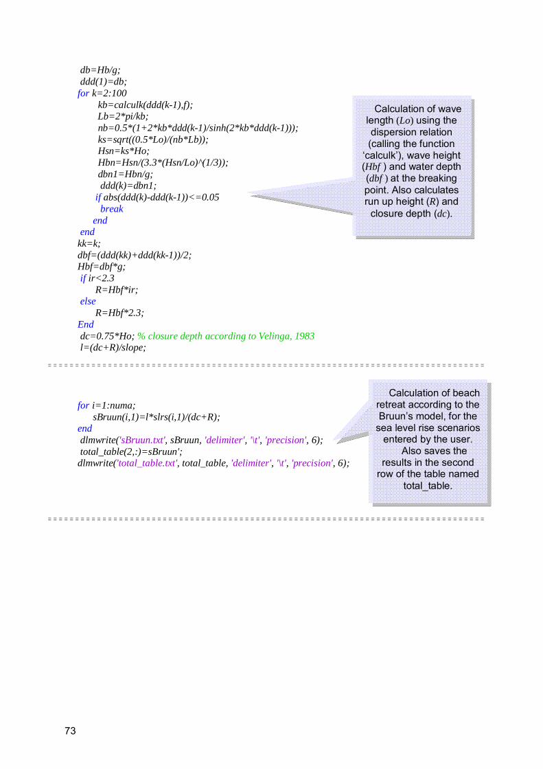
73
db=Hb/g; ddd(1)=db; for k=2:100 kb=calculk(ddd(k-1),f); Lb=2*pi/kb; nb=0.5*(1+2*kb*ddd(k-1)/sinh(2*kb*ddd(k-1))); ks=sqrt((0.5*Lo)/(nb*Lb)); Hsn=ks*Ho; Hbn=Hsn/(3.3*(Hsn/Lo)^(1/3)); dbn1=Hbn/g; ddd(k)=dbn1; if abs(ddd(k)-ddd(k-1))<=0.05 break end end kk=k; dbf=(ddd(kk)+ddd(kk-1))/2; Hbf=dbf*g; if ir<2.3 R=Hbf*ir; else R=Hbf*2.3; End dc=0.75*Ho; % closure depth according to Velinga, 1983 l=(dc+R)/slope; for i=1:numa; sBruun(i,1)=l*slrs(i,1)/(dc+R); end dlmwrite('sBruun.txt', sBruun, 'delimiter', '\t', 'precision', 6); total_table(2,:)=sBruun'; dlmwrite('total_table.txt', total_table, 'delimiter', '\t', 'precision', 6);
Calculation of wave length (Lo) using the dispersion relation (calling the function
‘calculk’), wave height (Hbf ) and water depth (dbf ) at the breaking point. Also calculates run up height (R) and
closure depth (dc).
Calculation of beach retreat according to the Bruun’s model, for the
sea level rise scenarios entered by the user.
Also saves the results in the second
row of the table named total_table.

74
% --- Executes on button press in Dmodel. function Dmodel_Callback(hObject, eventdata, handles) % hObject handle to Dmodel (see GCBO) % eventdata reserved - to be defined in a future version of MATLAB % handles structure with handles and user data (see GUIDATA) m=str2num(get(handles.Slope,'String')); Ho=str2num(get(handles.Wheight,'String')); T=str2num(get(handles.Wperiod,'String')); load slrs.txt; load total_table.txt; numa=size(slrs,1); slope=1/m; do=20; f=1/T; kl=calculk(do,f); Lo=2*pi/kl; ir=slope/sqrt(Ho/Lo); Hs=Ho; Hb=Hs/(3.3*(Hs/Lo)^(1/3)); g=ir^0.17+0.08; db=Hb/g; ddd(1)=db; for k=2:100 kb=calculk(ddd(k-1),f); Lb=2*pi/kb; nb=0.5*(1+2*kb*ddd(k-1)/sinh(2*kb*ddd(k-1))); ks=sqrt((0.5*Lo)/(nb*Lb)); Hsn=ks*Ho; Hbn=Hsn/(3.3*(Hsn/Lo)^(1/3)); dbn1=Hbn/g; ddd(k)=dbn1; if abs(ddd(k)-ddd(k-1))<=0.05 break end end kk=k; dbf=(ddd(kk)+ddd(kk-1))/2; Hbf=dbf*g; if ir<2.3 R=Hbf*ir; else R=Hbf*2.3;
Gets the input values for the beach
slope (m), wave height (Ho) and wave period
(T) entered by the user. Also loads the file
‘slrs.txt’ which contains the sea level rise
scenarios entered by the user.
Calculation of wave length (Lo) using the dispersion relation (calling the function
‘calculk’), wave height (Hbf ) and water depth (dbf ) at the breaking
point. Also calculates run up height (R) and the width of the surf zone
(wb).
The function executed with the press of pushbutton ‘Run’ under the text field ‘Dean’:

75
end Wb=dbf/slope; for i=1:numa; sDean(i,1)=(slrs(i)+0.068*Hbf)*Wb/(R+dbf); end; save sDean sDean; dlmwrite('sDean.txt', sDean, 'delimiter', '\t', 'precision', 6); total_table(1,:)=sDean'; dlmwrite('total_table.txt', total_table, 'delimiter', '\t', 'precision', 6);
% --- Executes on button press in Edeltable. function Edeltable_Callback(hObject, eventdata, handles) % hObject handle to Edeltable (see GCBO) % eventdata reserved - to be defined in a future version of MATLAB % handles structure with handles and user data (see GUIDATA) load sEdel.txt; load slrs.txt; aa(:,1)=slrs; aa(:,2)=sEdel; ss=num2str(aa); msgbox(ss,'Edelman')
Calculation of beach retreat according to the Dean’s model, for the
sea level rise scenarios entered by the user.
Also saves the results in the third row
of the table named total_table.
The function executed with the press of pushbutton ‘View results’ e.g. for the model Edelman:
Creates a table consisted of 2 columns. The 1st column shows the sea level rise scenarios selected by the user, the 2nd column shows the beach retreat estimations for these
scenarios resulted from e.g. Edelman model.
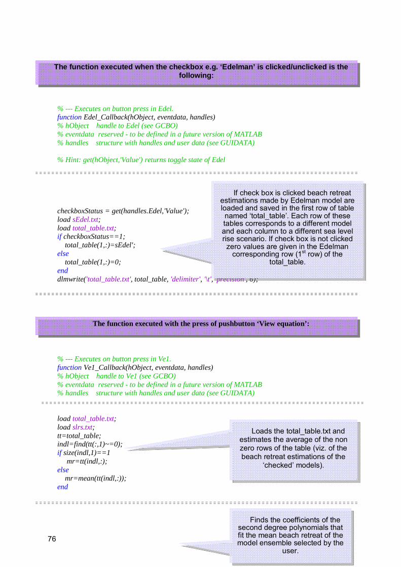
76
% --- Executes on button press in Edel. function Edel_Callback(hObject, eventdata, handles) % hObject handle to Edel (see GCBO) % eventdata reserved - to be defined in a future version of MATLAB % handles structure with handles and user data (see GUIDATA) % Hint: get(hObject,'Value') returns toggle state of Edel checkboxStatus = get(handles.Edel,'Value'); load sEdel.txt; load total_table.txt; if checkboxStatus==1; total_table(1,:)=sEdel'; else total_table(1,:)=0; end dlmwrite('total_table.txt', total_table, 'delimiter', '\t', 'precision', 6);
% --- Executes on button press in Ve1. function Ve1_Callback(hObject, eventdata, handles) % hObject handle to Ve1 (see GCBO) % eventdata reserved - to be defined in a future version of MATLAB % handles structure with handles and user data (see GUIDATA) load total_table.txt; load slrs.txt; tt=total_table; indl=find(tt(:,1)~=0); if size(indl,1)==1 mr=tt(indl,:); else mr=mean(tt(indl,:)); end
The function executed when the checkbox e.g. ‘Edelman’ is clicked/unclicked is the following:
If check box is clicked beach retreat
estimations made by Edelman model are loaded and saved in the first row of table named ‘total_table’. Each row of these tables corresponds to a different model and each column to a different sea level rise scenario. If check box is not clicked zero values are given in the Edelman
corresponding row (1st row) of the total_table.
The function executed with the press of pushbutton ‘View equation’:
Loads the total_table.txt and estimates the average of the non zero rows of the table (viz. of the beach retreat estimations of the
‘checked’ models).
Finds the coefficients of the
second degree polynomials that fit the mean beach retreat of the model ensemble selected by the
user.

77
pr=polyfit(slrs',mr,2); yr=pr(1)*(slrs.^2)+pr(2)*slrs+pr(3); rss_r=sum((yr-mr').^2); sss_r=sum((mr-mean(mr)).^2); rr_r=1-rss_r/sss_r; cresr1(1,:)=char(['s= p1 x a^2 + p2 x a + p3 ']); cresr2(1,:)=char([' p1 = ' num2str(pr(1))]); cresr3(1,:)=char([' p2 = ' num2str(pr(2))]); cresr4(1,:)=char([' p3 = ' num2str(pr(3))]); cresr5(1,:)=char([' R^2 = ' num2str(rr_r) '']); cresr6(1,:)=char(['s = beach retreat (m) ']); cresr7(1,:)=char(['a = sea level rise (m)']); set(handles.eq1,'String',cresr1(1,:)); set(handles.eq2,'String',cresr2(1,:)); set(handles.eq3,'String',cresr3(1,:)); set(handles.eq4,'String',cresr4(1,:)); set(handles.eq5,'String',cresr5(1,:)); set(handles.eq6,'String',cresr6(1,:)); set(handles.eq7,'String',cresr7(1,:));
% --- Executes on button press in plres. function plres_Callback(hObject, eventdata, handles) % hObject handle to plres (see GCBO) % eventdata reserved - to be defined in a future version of MATLAB % handles structure with handles and user data (see GUIDATA) load total_table.txt; load slrs.txt; tt=total_table; indl=find(tt(:,1)~=0); if size(indl,1)==1 mr=tt(indl,:); else mr=mean(tt(indl,:)); end pr=polyfit(slrs',mr,2); yr=pr(1)*(slrs.^2)+pr(2)*slrs+pr(3); for i=1:size(indl,1);
The function executed with the press of pushbutton ‘Plot results’:
Finds the
coefficients of the second degree
polynomials that fit the beach retreat
projections of the models selected by the
user.
Creates the text strings that describes the
polynomial equation fitted to the mean beach retreat
estimations of the ensemble of the models
selected by the user.
Displays the text strings created at the previous step in the
fields under the push button ‘View equation’.

78
ppr(i,:)=polyfit(slrs',tt(indl(i),:),2); yyr(i,:)=ppr(i,1)*(slrs.^2)+ppr(i,2)*slrs+ppr(i,3); end colo=['r','k','b','g','k']; typ=['-',':','-','-','-']; tit(1,:)=char(['Edelman ']); tit(2,:)=char(['Bruun ']); tit(3,:)=char(['Dean ']); tit(4,:)=char(['Mean ']); indnl=[indl;4]; figure for i=1:size(indl,1); pl=plot([0;slrs],[0;yyr(i,:)'],typ(i)); set(pl,'color',colo(i)); hold on; end if size(indl,1)==1; hold off; indnl=indl; else h=plot([0;slrs],[0;yr],'--'); set(h,'color',[0.6 0.2 0],'linewidth',2); indnl=[indl;4]; end set(gca,'fontsize',15); xlabel('Sea level rise (m)','fontsize',22); ylabel('Beach retreat (m)','fontsize',22); legend(tit(indnl,:),'location','northwest'); axis tight; grid on;
% --- Executes on button press in calc. function calc_Callback(hObject, eventdata, handles) % hObject handle to calc (see GCBO) % eventdata reserved - to be defined in a future version of MATLAB % handles structure with handles and user data (see GUIDATA) slr=str2num(get(handles.slr1,'String')); load total_table.txt; load slrs.txt;
The function executed with the press of pushbutton ‘Calculate’:
Calculates the beach retreat for a specific sea level rise
scenario given by the user, in the edit box with the Tag name ‘slr1’ next to the text ‘Sea level
rise:’ using the polynomial equations that describe the
mean (of the selected models)
Plots the polynomials found for the selected models
together with the polynomial of the mean
of these models.

79
tt=total_table; indl=find(tt(:,1)~=0); if size(indl,1)==1 mr=tt(indl,:); else mr=mean(tt(indl,:)); end pr=polyfit(slrs',mr,2); yr=pr(1)*(slr.^2)+pr(2)*slr+pr(3); br1=roundn(yr,-3); set(handles.bretreat1,'String',br1);
80
References
Bascom, W. N., 1964, Waves and Beaches., Doubleday, Garden City, New York. Battjes, J. A., and Janssen, J. P. F. M., 1978, Energy loss and set-up due to breaking in
random waves, in: 16th International Conference on Coastal Engineering, ASCE, Hamburg, pp. 569-587.
Bruun, P., 1988, The Bruun Rule of erosion by sea level rise: A discussion on large-scale two- and three-dimensional usages, Journal of Coastal Research 4(4):622-648.
Dean, R. G., 1991, Equilibrium beach profiles: characteristics and applications, J. Coastal Research 7(1):53– 84.
Dean, R. G., 2002, Beach nourishment: Theory and practice, in: Advanced Series on Ocean Engineering, Singapore: World Scientific Publishing Company.
Edelman, T., 1972, Dune erosion during storm conditions, in: Proceedings of the 13th International Conference on Coastal Engineering ASCE, pp. 1305-1312.
Komar, P. D., 1998, Beach Processes and Sedimentation, Prentice Hall, N.J., USA, pp. 544. Larson, M., and Kraus, N. C., 1989, SBEACH: numerical model for simulating storm-induced
beach change; report 1: empirical foundation and model development, Technical Report - US Army Coastal Engineering Research Center 89-9.
Leont'yev, I. O., 1996, Numerical modelling of beach erosion during storm event, Coastal Engineering 29(1-2):187-200.
McLeod, E., Poulter, B., Hinkel, J., Reyes, E., and Salm, R., 2010, Sea-level rise impact models and environmental conservation: A review of models and their applications, Ocean and Coastal Management 53(9):507-517.
Nicholls, R. J., Wong, P. P., Burkett, V. R., Codignotto, J. O., Hay, J. E., McLean, R. F., Ragoonaden, S., and Wooddroffe, C. D., 2007, Impacts, Adaptation, and Vulnerability. Contribution of Working Group II to the Fourth Assessment Report of the Intergovernmental Panel of Climate Change. (Parry M.L., O. F. Canziani, J. P. Palutikof, P. J. Van de Linden, and C. E. Hanson, eds.), Cambridge University Press, Cambridge, UK, pp. 315-356.
Niedoroda, A. W., Resio, D. T., Toro, G. R., Divoky, D., Das, H. S., and Reed, C. W., 2009, Analysis of the coastal Mississippi storm surge hazard, Ocean Engineering (in press).
Nielsen, P., 1992. Coastal Bottom Boundary Layers and Sediment Transport. Advanced Series on Ocean Engineering, 4. Word Scientific 324.
Roelvink, J. A., Stive, M.J.F., 1989, Bar-generating cross-shore flow mechanisms on a beach, Journal of Geophysical Research 94(C4):4785– 4800.
Van Rijn, L. C., Walstra, D. J. R., Grasmeijer, B., Sutherland, J., Pan, S., and Sierra, J. P., 2003, The predictability of cross-shore bed evolution of sandy beaches at the time scale of storms and seasons using process-based Profile models, Coastal Engineering 47(3):295-327.
Zhang, K., Douglas, B. C., and Leatherman, S. P., 2004, Global warming and coast erosion, Climate Change 64:41-58.

81
Beach Retreat under Sea Level Rise
The main objectives of this part of the Training Session are (a) to transfer ‘know how’
developed within the RiVAMP and (b) provide free platforms/software solutions to Jamaican
and Caribbean’s partners with regard to a rapid assessment of beach erosion/retreat under
climate change-induced sea level rise. This part of the Training forms an integral part of the
overarching objective of the RiVAMP Training Session, i.e. to promote an improved
understanding of the role of ecosystems in disaster risk reduction (including climate change-
related risks), through integrated assessments that can support policy and land-use planning
decisions.
Climate change induces several impacts pertinent to coastal areas, including mean sea
level rise, warmer water temperatures, higher intensity of cyclones, storm surges and
precipitation as well as changes in the wave regime (e.g. Emanuel, 2005; Allan.and Soden,
2008; and Ruggiero et al., 2010). These changes can severely affect coastal ecosystems
and economic activities, such as e.g. coral reefs (e.g. Woodroffe, 2008), coastal wetlands,
seagrasses and lagoons (e.g. Cruz-Palacios and van Tussenbroek, 2005; Karim and
Mimura, 2008), beaches (McKee Smith et al., 2010) , tourism (e.g Bardolet and Sheldon,
2008), seaports and other coastal infrastructure (e.g. Nicholls et al., 2007; McGranahan et
al., 2007; CCSP, 2008; Lenton et al., 2009), particularly in Developing Countries and SIDS
(e.g. Dasgupta et al., 2009). However, although predictions of exposure to climatic changes
are required at decadal scales, most of the available information/models are dealing with
either long-term (century-to millennium) (e.g. Nott et al, 2009), annual (e.g. Greenwood and
Orford, 2008) or even storm event (e.g. Callaghan et al., 2008) scales. There have already
been attempts to develop global coastal hazards data bases (e.g. Vafeidis et al., 2008), as
well as methodologies/tools to assess rapidly coastal vulnerability to sea level rise and
extreme events (e.g. Hinkel and Klein, 2009), but the work is still far from concluded
(McLeod et al., 2010).
Within the RiVAMP framework, a simple, rapid methodology has been applied/used (e.g.
Estrella et al., 2010) to assess beach retreat/erosion under both-long- and short term sea
level rise (see also Velegrakis et al., 2009). According to this method, ensembles of beach
morphodynamic models of varying complexity are used in order to assess
beach/erosion/retreat under varying conditions (i.e. beach slope and sediment size) and
forcing (i.e. sea level rise and wave conditions). In the present RiVAMP Training Session, an
especially developed tool, based on the construction/application of ensembles (a short-term
and a long-term ensemble) of different 1-D analytical and numerical morphodynamic models

82
of varied complexity, will be presented/distributed that can rapidly estimate ranges of beach
retreat for different morphologically and sedimentologically beaches, under different
scenarios of long-term and short-term sea level rise and different hydrodynamic forcing. It
must be noted that this tool does not intend to replace detailed studies, which are based
upon the 2-D/3-D morphodynamic modles calibrated/validated through the collection of
comprehensive sets of field observations, but to provide an easily deployed methodology that
can provide a rapid first assessment of beach erosion/inundation risks under sea level rise.
References Allan RP and BJ Soden, 2008, Atmospheric warming and the amplification of precipitation extremes.
Science 321, 1481-1484. Bardolet, E. and P.J. Sheldon, 2008. Tourism in archipelagos: Hawai’i and the Balearics
Annals of Tourism Research, 35, 900-923 Callaghan DP, P Nielsen, A Short and R Ranasinghe, 2008. Statistical simulation of wave climate and
extreme beach erosion. Coastal Engineering, 55, 375–390. CCSP, 2008. Impacts of Climate Change and Variability on Transportation Systems and Infrastructure:
Gulf Coast Study, Phase I. A Report by the U.S. Climate Change Science Program and the Subcommittee on Global Change Research [Savonis MJ, VR Burkett, and JR Potter (eds.)]. Department of Transportation, Washington, DC, USA, 445 pp.
Cruz-Palacios, V. and B. I. van Tussenbroek, 2005. Simulation of hurricane-like disturbances on a Caribbean seagrass bed. Journal of Experimental Marine Biology and Ecology, 324, 44-60.
Dasgupta S, B Laplante, S Murray and D Wheeler, 2009. Sea-Level Rise and Storm Surges: A Comparative Analysis of Impacts in Developing Countries. Policy Research Working Paper 4901, the World Bank Development Research Group, Environment and Energy Team. 41pp.
Emanuel, K., 2005: Increasing destructiveness of tropical cyclones over the past 30 years. Nature, 436, 686-688.
Estrella, M., Peducci, P., Velegrakis, A.F., Chatenoux, B., Kluser, S., 2010. Linking Ecosystems to Risk and Vulnerability Reduction: The Case of Jamaica. Technical Report of the Risk and Vulnerability Assessment Methodology Development Project (RiVAMP), UNEP. 100 pp.
Greenwood RO and JD Orford, 2008. Temporal patterns and processes of retreat of drumlin coastal cliffs — Strangford Lough, Northern Ireland Geomorphology, 94, 153-169.
Hinkel J. and RJT Klein, 2009. Integrating knowledge to assess coastal vulnerability to sea-level rise: The development of the DIVA tool. Global Environmental Change, 19, 384-395.
Karim, F.M.and N. Mimura, 2008. Impacts of climate change and sea-level rise on cyclonic storm surge floods in Bangladesh. Global Environmental Change, 18, 490-500.
Lenton TM, A Footitt and A Dlugolecki, 2009. Major Tipping Points in the Earth’s Climate System and Consequences for the Insurance Sector. WWF, Gland, Switzerland and Allianz SE, Munich, Germany.
McGranahan, G., D. Balk and B. Anderson, 2007. The Rising Tide: Assessing the Risks of Climate Change and Human settlements in Low Elevation Coastal Zones. Environment & Urbanization Copyright © 2007 International Institute for Environment and Development (IIED).Vol 19(1): 17–37. DOI: 10.1177/0956247807076960.
McKee Smith, J., M.A. Cialone, T.V. Wamsley, T.O. McAlpin, 2010. Potential impact of sea level rise on coastal surges in southeast Louisiana. Ocean Engineering, 37, 37–47
McLeod, E., Poulter, B., Hinkel, J., Reyes, E., and Salm, R., 2010, Sea-level rise impact models and environmental conservation: A review of models and their applications, Ocean and Coastal Management 53(9):507-517.
Nicholls RJ, PP Wong, VR Burkett, JO Codignotto, JE Hay, RF McLean, S Ragoonaden, and CD Woodroffe, 2007. Coastal systems and low-lying areas. In: Climate change 2007: Impacts, Adaptation, and Vulnerability. Contribution of Working Group II to the Fourth Assessment Report of the Intergovernmental Panel of Climate Change. [Parry M, OF Canziani, JP Palutikof, PJ Van der Linden,and CE Hanson (eds.)]. Cambridge University Press, Cambridge, UK, 315-356.

83
Nott JS, J Smithers, K Walsh and E. Rhodes, 2009. Sand beach ridges record 6000 year history of extreme tropical cyclone activity in northeastern Australia. Quarternary Science Reviews, 28, 1511–1520.
Ruggiero P, PD Komar and JC Allan, 2010. Increasing wave heights and extreme value projections: The wave climate of the U.S. Pacific Northwest. Coastal Engineering, 57, 539–552.
Velegrakis, A.F., Lehmann, A., Monioudi, I, Giuliani, G., Herold, C., Allenbach, A., De Bono, A. and Radchenko, I., 2009. Beach erosion prediction for the Black Sea coast, due to sea level rise. Proceedings of the 9th MEDCOAST Conf., Sochi, Russia, 10-14 Nov, 2009, 776-787.
Woodroffe, C.D., 2008. Reef-island topography and the vulnerability of atolls to sea-level rise. Global and Planetary Change 62, 77–96.