traffic control device analysis, testing, and evaluation

Cooperative Research Program

TTI: 0-6969

Technical Report 0-6969-R3

Traffic Control Device Analysis, Testing, and

Evaluation Program: FY2020 Activities

in cooperation with the

Federal Highway Administration and the

Texas Department of Transportation

http://tti.tamu.edu/documents/0-6969-R3.pdf

TEXAS A&M TRANSPORTATION INSTITUTE

COLLEGE STATION, TEXAS

Technical Report Documentation Page 1. Report No.

FHWA/TX-21/0-6969-R3

2. Government Accession No.

3. Recipient's Catalog No.

4. Title and Subtitle

TRAFFIC CONTROL DEVICE ANALYSIS, TESTING, AND

EVALUATION PROGRAM: FY2020 ACTIVITIES

5. Report Date

Published: June 2021 6. Performing Organization Code

7. Author(s)

Melisa D. Finley, Adam M. Pike, Kay Fitzpatrick, Eun Sug Park,

LuAnn Theiss, Michael P. Pratt, Nadeem Chaudhary, Srinivasa

Sunkari, Nick Wood, and Songjukta Datta

8. Performing Organization Report No.

Report 0-6969-R3

0 9. Performing Organization Name and Address

Texas A&M Transportation Institute

The Texas A&M University System

College Station, Texas 77843-3135

10. Work Unit No. (TRAIS)

11. Contract or Grant No.

Project 0-6969 12. Sponsoring Agency Name and Address


Research and Technology Implementation Office

125 E. 11th Street

Austin, Texas 78701-2483

13. Type of Report and Period Covered

Technical Report:

September 2019–August 2020 14. Sponsoring Agency Code

15. Supplementary Notes

Project performed in cooperation with the Texas Department of Transportation and the Federal Highway

Administration.

Project Title: Traffic Control Device Analysis, Testing, and Evaluation Program

URL: http://tti.tamu.edu/documents/0-6969-R3.pdf 16. Abstract

This project provides the Texas Department of Transportation with a mechanism to conduct high-priority,

limited-scope evaluations of traffic control devices. Work conducted and concluded during the 2020 fiscal

year included:

• Review of retroreflective raised pavement marker practices.

• Review of optical speed bar practices in horizontal curves.

• Review of traffic signal head backplate practices.

• Review of intersection conflict warning system practices.

• Development of guidance for the application of 6-inch pavement markings.

• Assessment of the effectiveness of work zone signing.

• Assessment of the effectiveness of pedestrian crossing treatments at night.

17. Key Words

Traffic Control Device, Retroreflective Raised

Pavement Marker, Optical Speed Bar, Traffic Signal

Head Backplate, Intersection Conflict Warning

System, Pavement Marking, Work Zone Signing,

Pedestrian Treatment, Pedestrian Hybrid Beacon,

Rectangular Rapid Flashing Beacon, Light Emitting

Diode Sign

18. Distribution Statement

No restrictions. This document is available to the

public through NTIS:

National Technical Information Service

Alexandria, Virginia

http://www.ntis.gov

19. Security Classif. (of this report)

Unclassified

20. Security Classif. (of this page)

Unclassified

21. No. of Pages

138

22. Price

Form DOT F 1700.7 (8-72) Reproduction of completed page authorized

TRAFFIC CONTROL DEVICE ANALYSIS, TESTING, AND

EVALUATION PROGRAM: FY2020 ACTIVITIES

by

Melisa D. Finley, P.E.

Research Engineer


Adam M. Pike, P.E.

Associate Research Engineer


Kay Fitzpatrick, Ph.D., P.E., PMP

Senior Research Engineer


Eun Sug Park, Ph.D.

Senior Research Scientist


LuAnn Theiss, P.E., PTOE, PMP

Research Engineer


Michael P. Pratt, P.E.

Assistant Research Engineer


Nadeem Chaudhary, Ph.D., P.E.

Senior Research Engineer


Srinivasa Sunkari, P.E., PMP

Research Engineer


Nick Wood, P.E.

Assistant Research Engineer


and

Songjukta Datta

Graduate Assistant Researcher


Report 0-6969-R3

Project 0-6969

Project Title: Traffic Control Device Analysis, Testing, and Evaluation Program

Performed in cooperation with the


and the

Federal Highway Administration

Published: June 2021

TEXAS A&M TRANSPORTATION INSTITUTE

College Station, Texas 77843-3135

v

DISCLAIMER

This research was performed in cooperation with the Texas Department of Transportation

(TxDOT) and the Federal Highway Administration (FHWA). The contents of this report reflect

the views of the authors, who are responsible for the facts and the accuracy of the data presented

herein. The contents do not necessarily reflect the official view or policies of FHWA or TxDOT.

This report does not constitute a standard, specification, or regulation.

This report is not intended for construction, bidding, or permit purposes. The engineer in charge

of this project was Melisa D. Finley, P.E. #TX-90937.

vi

ACKNOWLEDGMENTS

This project was conducted in cooperation with TxDOT and FHWA. Wade Odell of TxDOT

served as the project manager. The authors gratefully acknowledge the assistance and direction

that the TxDOT Project Monitoring Committee (PMC) provided over the course of the project.

The members of the PMC included:

• Nick Aiello.

• John Bassett.

• America Garza.

• James Keener.

• Jose Madrid.

• Kassondra Munoz.

• Barbara Russell.

• Doug Skowronek.

• Rebecca Wells.

The Texas A&M Transportation Institute (TTI) researchers would also like to acknowledge the

contributions of the many other TTI staff who assisted with various aspects of this project.

vii

TABLE OF CONTENTS

Page

List of Figures ................................................................................................................................ x List of Tables ............................................................................................................................... xii Chapter 1: Introduction ............................................................................................................... 1 Chapter 2: RRPM Use in Horizontal Curves and RRPM Spacing .......................................... 3

RRPMs along Edge Lines in Horizontal Curves ........................................................................ 3

Effectiveness of RRPMs at 40 ft versus 80 ft ........................................................................... 10 Current TxDOT Practices ..................................................................................................... 10 Operational-Related Studies ................................................................................................. 11

Safety-Related Studies .......................................................................................................... 13 Visibility-Related Studies ..................................................................................................... 15

Summary ................................................................................................................................... 19

Chapter 3: Optical Speed Bar Practices in Horizontal Curves .............................................. 21 Literature Review ..................................................................................................................... 21

Operational Effects of Optical Speed Bars ........................................................................... 22

Official Guidance for Optical Speed Bars ............................................................................ 26 Best Practices ............................................................................................................................ 27

Texas MUTCD Guidance ..................................................................................................... 27 Additional Guidance ............................................................................................................. 29 Incorporation of Optical Speed Bars into Guidance Frameworks ........................................ 30

Chapter 4: Traffic Signal Backplate Practices ......................................................................... 33 Case Studies .............................................................................................................................. 34

Winston-Salem ...................................................................................................................... 34 British Columbia ................................................................................................................... 34

Kentucky ............................................................................................................................... 35 Kansas ................................................................................................................................... 35

South Carolina ...................................................................................................................... 35 State Department of Transportation Practices .......................................................................... 36

Alabama ................................................................................................................................ 36 Florida ................................................................................................................................... 36

Kentucky ............................................................................................................................... 37 Louisiana ............................................................................................................................... 38 Maine .................................................................................................................................... 38 Nevada .................................................................................................................................. 38

Ohio ....................................................................................................................................... 39 Pennsylvania ......................................................................................................................... 40 Virginia ................................................................................................................................. 40

Washington ........................................................................................................................... 42 Chapter 5: Intersection Conflict Warning System Practices .................................................. 43

Background ............................................................................................................................... 43 Atlanta District Site Characteristics .......................................................................................... 46 Atlanta District ICWS ............................................................................................................... 51

Intersection Improvements .................................................................................................... 51

viii

Major-Street Approaches ...................................................................................................... 53 Minor-Street Approaches ...................................................................................................... 54

Equipment Installed .............................................................................................................. 56 Chapter 6: Guidance for the Application of 6-Inch Pavement Markings ............................. 59

National-Level Standards and Updates ..................................................................................... 59 MUTCD Definition ............................................................................................................... 59 NCUTCD-Approved Changes to the MUTCD Definition ................................................... 59

Past Research on Pavement Marking Width ............................................................................. 60 Impact of Wider Markings on Vehicle Operations ............................................................... 61 Impact of Wider Markings on Safety .................................................................................... 62 Impact of Wider Markings on Visibility ............................................................................... 64

State Practice on Marking Width .............................................................................................. 65

TxDOT Pavement Marking Cost Comparison ......................................................................... 66

Discussion and Recommendations ........................................................................................... 69 Chapter 7: Assessment of Effectiveness of Work Zone Signing ............................................. 73

Methodology ............................................................................................................................. 73

Identification of Work Zones ................................................................................................ 73 Work Zone Reviews ............................................................................................................. 74

Data Analysis ............................................................................................................................ 74

Results ....................................................................................................................................... 75 Spacing of Signage ............................................................................................................... 76

Truck Access Points .............................................................................................................. 78 Shoulder Reductions/Closures .............................................................................................. 81 Inconsistent Sequence and Placement of Guide Signs ......................................................... 83

Recommendations ..................................................................................................................... 86

Spacing of Signage ............................................................................................................... 86 Truck Access Points .............................................................................................................. 87 Shoulder Reductions/Closures .............................................................................................. 87

Inconsistent Sequence and Placement of Guide Signs ......................................................... 87 Chapter 8: Effectiveness of Pedestrian Crossing Treatments at Night ................................. 89

Previous Research ..................................................................................................................... 90 PHBs ..................................................................................................................................... 90 RRFBs ................................................................................................................................... 90

LED-Ems .............................................................................................................................. 91 Key Findings from Literature ............................................................................................... 91

Study Approach ........................................................................................................................ 91

Site Selection ........................................................................................................................ 92 Site Characteristics ................................................................................................................ 92

Data Collection Protocol ....................................................................................................... 95 Data Collection ..................................................................................................................... 96 Video Data Reduction ........................................................................................................... 97

Analysis .................................................................................................................................... 99 Results ..................................................................................................................................... 100

Average Driver Yielding Rate per Site ............................................................................... 100 ANCOVA Model Based on Mean Yield Rates for Sites and Light Level ......................... 102 PHB ..................................................................................................................................... 107

ix

RRFB .................................................................................................................................. 108 LED-Em .............................................................................................................................. 110

Conclusions ............................................................................................................................. 113 References .................................................................................................................................. 115

x

LIST OF FIGURES

Page

Figure 1. TxDOT District Use of RRPMs along the Outside Edges of Horizontal Curves. .......... 4 Figure 2. Atlanta District I-30 Curve (Source: © 2020 Google Earth). ......................................... 5 Figure 3. Atlanta District I-30 Curve in Street View (Source: © 2020 Google Earth). ................. 5 Figure 4. Pharr District US 281 Corridor (Source: © 2020 Google Earth). .................................. 6 Figure 5. Pharr District US 281 Corridor in Street View (Source: © 2020 Google Earth). .......... 6

Figure 6. San Antonio District I-37 Corridor (Source: © 2020 Google Earth).............................. 7 Figure 7. San Antonio District I-37 Corridor in Street View (Source: © 2020 Google

Earth). ..................................................................................................................................... 7

Figure 8. San Antonio District FM 471 Curve near Lacoste (Source: © 2020 Google

Earth). ..................................................................................................................................... 8 Figure 9. San Antonio District FM 471 Curve near Lacoste in Street View (Source: ©

2020 Google Earth). ............................................................................................................... 8 Figure 10. San Antonio District FM 471 Curve near PR 3810 (Source: © 2020 Google

Earth). ..................................................................................................................................... 9

Figure 11. San Antonio District FM 471 Curve near PR 3810 in Street View (Source:

© 2020 Google Earth). ........................................................................................................... 9

Figure 12. TxDOT District RRPM Spacing for Supplementing Broken Lane Line

Pavement Markings. ............................................................................................................. 11 Figure 13. Comparison of VL between RRPMs and Markings. ................................................... 17

Figure 14. RRPM VL Based on Low-Level Luminance. ............................................................. 18 Figure 15. RRPM VL Based on Half the Low-Level Luminance. ............................................... 18

Figure 16. RRPM VL Based on Half the Low-Level Luminance and Glare. .............................. 19 Figure 17. Texas MUTCD–Compliant Optical Speed Bars (22). ................................................. 22

Figure 18. Other Types of Optical Speed Bars (22). .................................................................... 22 Figure 19. Distribution of Speeds at Optical Speed Bar Test Sites (25). ..................................... 23

Figure 20. Herringbone-Pattern Optical Speed Bars (23). ............................................................ 24 Figure 21. Texas MUTCD Guidance on Application of Optical Speed Bars (2). ........................ 26 Figure 22. Horizontal Curve Signing Handbook Guidelines for Choosing Curve Traffic

Control Devices (32). ............................................................................................................ 29

Figure 23. ICWS Installation Site in Marshall, Texas (Source: © 2020 Google Earth). ............. 47 Figure 24. Speed Limits on the Major- and Minor-Street Approaches. ....................................... 48 Figure 25. Driver’s View at the Stop Lines on the Westbound Approach. .................................. 48 Figure 26. Drivers at the Stop Lines on the Eastbound Approach. ............................................... 49

Figure 27. Example of Treatments on the Minor-Street Approaches. .......................................... 50 Figure 28. Minor-Street Approach before ICWS (Source: © 2020 Google Earth). .................... 50 Figure 29. Major-Street Approach before ICWS (Source: © 2020 Google Earth). ..................... 51

Figure 30. Intersection Improvements on SL 390. ....................................................................... 52 Figure 31. Intersection Improvements on FM 1998. .................................................................... 52 Figure 32. Example of a Solar-Powered RFBA on the Major Street............................................ 53 Figure 33. Example of a Sensor to Detect Vehicles Approaching on the Minor Street. .............. 54 Figure 34. Example of a Warning Sign Assembly on the Minor Street (System Not

Activated). ............................................................................................................................. 55

xi

Figure 35. Example of a Sensor on the RFBA to Detect Vehicles Approaching on the

Major Street. ......................................................................................................................... 55

Figure 36. Example of a Warning Sign Assembly on the Minor Street (System

Activated). ............................................................................................................................. 56 Figure 37. Equipment Integrated at the Intersection. .................................................................... 57 Figure 38. Schematic of the ICWS. .............................................................................................. 57 Figure 39. Project Limit Signage (96). ......................................................................................... 74

Figure 40. Texas MUTCD Suggested Advance Warning Sign Spacing (2)................................. 76 Figure 41. Closely Spaced Signs at Site 1. ................................................................................... 77 Figure 42. Closely Spaced Signs at Site 3. ................................................................................... 77 Figure 43. R20-3T and G20-10T Signs (2, 100). .......................................................................... 78 Figure 44. Trucks Entering/Exiting Highway Sign at Site 3. ....................................................... 79

Figure 45. Trucks Entering/Exiting Roadway Sign at Site 4. ....................................................... 79

Figure 46. Trucks Entering Roadway Sign (CW27-1T) (100). .................................................... 80 Figure 47. Truck Entrance at Site 3. ............................................................................................. 80

Figure 48. Texas MUTCD Warning Signs for Shoulder Closures (2). ........................................ 81

Figure 49. Narrow Shoulder Ahead Warning Sign at Site 3......................................................... 82 Figure 50. Unpaved Shoulder Warning Sign at Site 3. ................................................................. 82 Figure 51. Right Shoulder Reduced Warning Sign at Site 4. ....................................................... 83

Figure 52. Interchange Exit Ramp Sign Sequence from Texas MUTCD (2). .............................. 84 Figure 53. Placement of Exit Direction Sign in Exit Gore. .......................................................... 85

Figure 54. Construction Plans Showing Placement of Exit Direction Sign. ................................ 85 Figure 55. Exit Direction and Exit Gore Signs at Site 4. .............................................................. 86 Figure 56. Exit Gore Sign Missing at Site 4. ................................................................................ 86

Figure 57. Examples of Treatments. ............................................................................................. 89

Figure 58. Example of Video Camera View. ................................................................................ 96 Figure 59. Driver Yielding by Treatment, Light Level, and Site. .............................................. 102 Figure 60. LSM Driver Yielding for Daytime and Nighttime by Treatment Type. ................... 105

Figure 61. LSM Driver Yielding for Speed Limit Groups by Treatment Type. ......................... 106 Figure 62. LSM Driver Yielding for Lane Width Group by Treatment Type. ........................... 106

Figure 63. Regression Plot for Mean Driver Yielding for PHB by Light Level. ....................... 108

xii

LIST OF TABLES

Page

Table 1. Optical Speed Bar Studies for Horizontal Curve Applications (24). .............................. 23 Table 2. Pavement Treatment Simulator Study Results (Adapted from 23). ............................... 25 Table 3. Optical Speed Bar Studies for Other Site Applications. ................................................. 26 Table 4. Horizontal Alignment Sign Selection (2). ...................................................................... 28 Table 5. Delineator and Chevron Guidance from the 2006 Texas MUTCD (31). ....................... 28

Table 6. Horizontal Curve Signing Handbook Guidelines for Choosing Curve Traffic

Control Devices (32). ............................................................................................................ 30 Table 7. Candidate Updated Horizontal Alignment Sign and Marking Selection. ....................... 31

Table 8. Impact of Signal Backplates with Retroreflective Border. ............................................. 36 Table 9. Crash Modification Factors from the FHWA ICWS Evaluation. ................................... 45 Table 10. Average Cost Estimates by Intersection Type (in 2014 Dollars). ................................ 46

Table 11. Summary of the Impact of Wider Pavement Markings on Safety. ............................... 63 Table 12. Summary of Pavement Marking Construction Cost. .................................................... 67 Table 13. Summary of Pavement Markings Maintenance Cost. .................................................. 68

Table 14. Summary of Pavement Marking Costs. ........................................................................ 68 Table 15. Data Collection Locations. ........................................................................................... 74

Table 16. Work Zone Sign Data Summary. .................................................................................. 75 Table 17. Variable Descriptions. .................................................................................................. 93 Table 18. Site Characteristics for the PHB Sites. ......................................................................... 94

Table 19. Site Characteristics for the RRFB Sites. ....................................................................... 94 Table 20. Site Characteristics for the LED-Em Sites. .................................................................. 95

Table 21. Number of Staged Pedestrian Crossings and Drivers Included in Analysis. ................ 97 Table 22. Hourly Vehicle Volume (Minimum, Maximum, and Average) Calculated

Based on 1-Minute Count Prior to Pedestrian Staged Crossing. .......................................... 98 Table 23. Average Driver Yielding Rate by Site for Daytime and Nighttime Conditions. ........ 101

Table 24. ANCOVA Model Including Treatment Type, Light Level, and Other Site

Characteristic Variables Using Per-Site Mean Yield Rates. ............................................... 103 Table 25. Fixed Effect Tests for Model in Table 24. .................................................................. 104 Table 26. LSM Differences Tukey HSD by Treatment Type and Light Level. ......................... 105

Table 27. LSM Differences Tukey HSD by Treatment Type and Speed Group. ....................... 106 Table 28. LSM Differences Tukey HSD by Treatment Type and Lane Width. ......................... 107 Table 29. ANCOVA Model Using Per-Site Mean Yield Rates at PHBs. .................................. 107 Table 30. Logistic Regression Based on Driver Response at PHBs. .......................................... 108

Table 31. ANCOVA Model Using Per-Site Mean Yield Rates at RRFBs. ................................ 109 Table 32. Logistic Regression Based on Driver Response at RRFBs. ....................................... 110 Table 33. ANCOVA Model Using Per-Site Mean Yield Rates at LED-Ems. ........................... 110

Table 34. Logistic Regression Based on Driver Response at LED-Ems. ................................... 112 Table 35. Contrast Estimate Results for LED-Ems. ................................................................... 112

1

CHAPTER 1:

INTRODUCTION

This project provides the Texas Department of Transportation (TxDOT) with a mechanism to

conduct high-priority, limited-scope evaluations of traffic control devices. Research activities

conducted during the 2020 fiscal year (September 2019–August 2020) included:

• Review of retroreflective raised pavement marker (RRPM) practices.

• Review of optical speed bar practices in horizontal curves.

• Review of traffic signal head backplate practices.

• Review of intersection conflict warning system practices.

• Development of guidance for the application of 6-inch pavement markings.

• Assessment of the effectiveness of signing in work zones.

• Assessment of the effectiveness of pedestrian crossing treatments at night.

• Evaluation of wet-weather pavement marking retroreflectivity.

• Evaluation of the design and application of driveway assistance devices in lane closures

on two-lane, two-way roads.

• Evaluation of shoulder rumble strip placement.

Researchers completed the first seven of these activities, and their findings are documented in

this report. The remaining three activities are ongoing and will be documented in future reports

under TxDOT Project 0-7096.

To inform decisions regarding traffic control device research needs and changes/updates to

TxDOT policies, procedures, and standards, researchers also conducted a two-stage survey of

practice to assess traffic control device practices and needs in TxDOT districts. In March 2020,

researchers, in cooperation with TxDOT Safety Division staff, developed and conducted a

preliminary online questionnaire to:

• Identify district center line striping practices when lateral separation is installed between

opposing travel directions (i.e., center line buffer).

• Identify what changes and additional guidance are needed in the TxDOT Rumble Strip

Standards.

• Identify districts installing wet-weather pavement markings.

• Identify district practices regarding RRPMs.

• Identify district traffic signal backplate practices.

Researchers then contacted district staff via email and phone in April and May 2020 to gather

more detailed information about district practices. Since the first three survey topics were

considered internal in nature or pertain to ongoing research activities, they are not documented

2

here. The district survey findings for the two remaining topics are included in their respective

chapters.

3

CHAPTER 2:

RRPM USE IN HORIZONTAL CURVES AND RRPM SPACING

For this activity, researchers reviewed TxDOT usage of RRPMs along edge lines in horizontal

curves and the effectiveness of RRPM spacing at 40 ft versus 80 ft. Researchers gauged TxDOT

usage of RRPMs along edge lines in horizontal curves through a survey of TxDOT districts.

Researchers assessed the effectiveness of RRPM spacing at 40 ft versus 80 ft for broken lane line

markings through a review of state practices, a survey of TxDOT districts, and a literature

review.

RRPMS ALONG EDGE LINES IN HORIZONTAL CURVES

The federal and Texas Manual on Traffic Control Devices (MUTCD) (1, 2) allow RRPMs to

supplement inside and outside edge lines. The specific language in Section 3B.13 states:

Raised pavement markers should not supplement right-hand edge lines unless an

engineering study or engineering judgment indicates the benefits of enhanced

delineation of a curve or other location would outweigh possible impacts on

bicycles using the shoulder, and the spacing of raised pavement markers on the

right-hand edge is close enough to avoid misinterpretation as a broken line during

wet night conditions.

This language indicates that engineering judgment or an engineering study can be used to justify

the use of RRPMs along the inside or outside edge line in curves or other areas where enhanced

delineation is desired. The RRPM edge line spacing should be no greater than N/2, which is 20 ft

for Texas. The presence of bicyclists in areas where outside edge lines are supplemented needs to

be considered.

There has been very little research on the operational impact, safety effectiveness, or visibility

benefits of supplementing edge line pavement markings with RRPMs. A few older research

studies that included RRPMs supplementing edge lines are described later in this chapter.

Intuitively, the addition of RRPMs to edge line markings should improve visibility and thus

improve lane-keeping ability. The enhanced delineation provided by the edge line RRPMs is

most likely to provide benefits at locations where maintaining lane position is critical. These

areas may include but are not limited to horizontal curves and approaches to bridges or other

points where a roadway narrows.

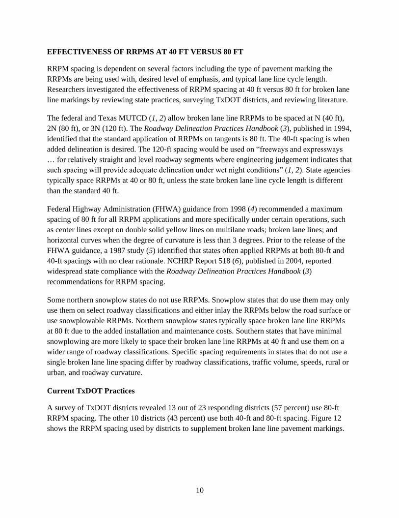
A survey of TxDOT districts revealed that 30 percent of the responding districts (seven out of

23) use RRPMs along the outside or inside edges of horizontal curves (see Figure 1). Several

districts responded with specific locations where RRPMs were installed along the outside edges

of horizontal curves. These locations included isolated curves and roadway corridors where

several curves were treated.

4

Figure 1. TxDOT District Use of RRPMs along the Outside Edges of Horizontal Curves.

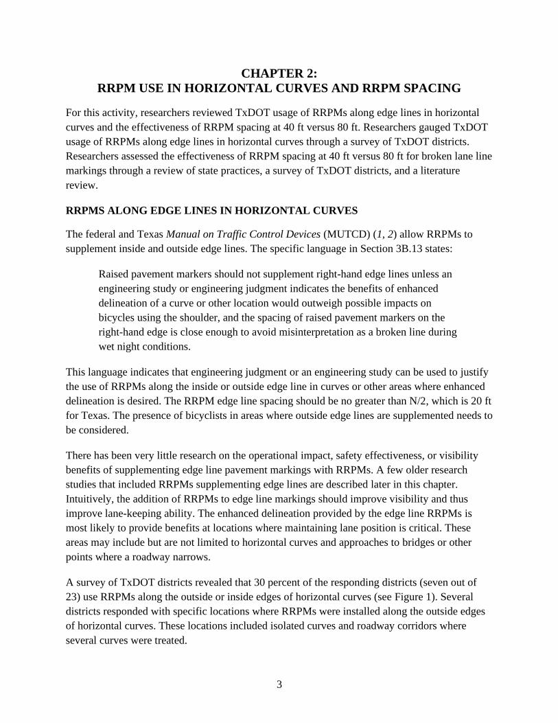
In March 2020, the Atlanta District installed RRPMs along the edges of a horizontal curve on

Interstate (I) 30 between Farm-to-Market (FM) 560 and FM 1398 in Bowie County near Hooks,

Texas (see Figure 2 and Figure 3). The Pharr District installed amber RRPMs on the outside

edge of horizontal curves on U.S. Highway (US) 281 in Hidalgo County (see Figure 4 and

Figure 5). The Pharr District placed the RRPMs adjacent to the yellow edge line between the

milled rumble strips in the curves and tangent leading up to the curve. The other tangent sections

in the corridor did not have supplemental RRPMs on the left shoulder.

The San Antonio District installed Type II-A-A RRPMs (i.e., two reflective faces oriented

180 degrees to each other, each of which must reflect amber light) along curved sections of I-37

between Spur 199 and Campbellton (approximately 11 miles) (see Figure 6 and Figure 7). The

San Antonio District RRPM application was like that of the Pharr District except that the

RRPMs were placed directly on the yellow edge line. The I-37 application appears to be for the

southbound travel direction only (based on Google Earth images). The San Antonio District also

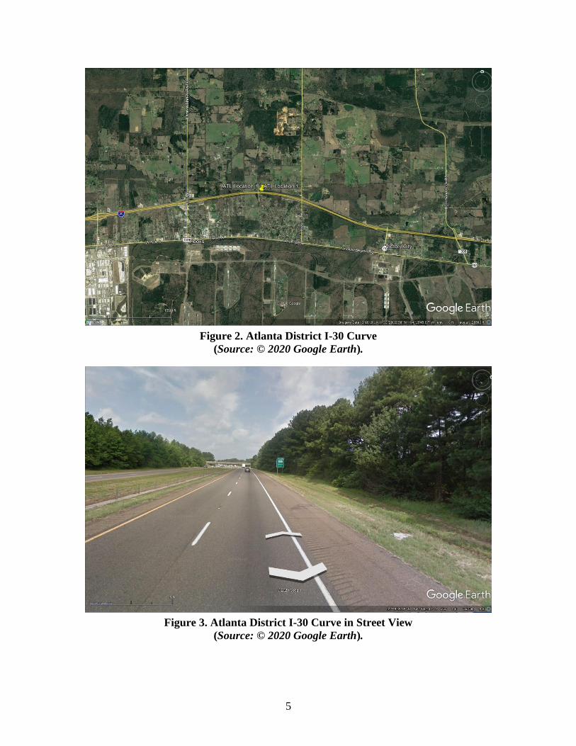
installed Type I-C RRPMs (i.e., one face that reflects white light) on the following two-lane

roads in Medina County:

• FM 471 southbound going into LaCoste, Texas (see Figure 8 and Figure 9).

• FM 471 northbound just south of private road (PR) 3810 (see Figure 10 and Figure 11).

The FM 471 application going into LaCoste was only for the direction of travel entering town.

The FM 471 application near PR 3810 was for both directions of travel. The Google Earth

images for this site show the RRPMs have been dislodged from the road surface.

5

Figure 2. Atlanta District I-30 Curve

(Source: © 2020 Google Earth).

Figure 3. Atlanta District I-30 Curve in Street View


6

Figure 4. Pharr District US 281 Corridor


Figure 5. Pharr District US 281 Corridor in Street View


7

Figure 6. San Antonio District I-37 Corridor


Figure 7. San Antonio District I-37 Corridor in Street View


8

Figure 8. San Antonio District FM 471 Curve near Lacoste


Figure 9. San Antonio District FM 471 Curve near Lacoste in Street View


9

Figure 10. San Antonio District FM 471 Curve near PR 3810


Figure 11. San Antonio District FM 471 Curve near PR 3810 in Street View


10

EFFECTIVENESS OF RRPMS AT 40 FT VERSUS 80 FT

RRPM spacing is dependent on several factors including the type of pavement marking the

RRPMs are being used with, desired level of emphasis, and typical lane line cycle length.

Researchers investigated the effectiveness of RRPM spacing at 40 ft versus 80 ft for broken lane

line markings by reviewing state practices, surveying TxDOT districts, and reviewing literature.

The federal and Texas MUTCD (1, 2) allow broken lane line RRPMs to be spaced at N (40 ft),

2N (80 ft), or 3N (120 ft). The Roadway Delineation Practices Handbook (3), published in 1994,

identified that the standard application of RRPMs on tangents is 80 ft. The 40-ft spacing is when

added delineation is desired. The 120-ft spacing would be used on “freeways and expressways

… for relatively straight and level roadway segments where engineering judgement indicates that

such spacing will provide adequate delineation under wet night conditions” (1, 2). State agencies

typically space RRPMs at 40 or 80 ft, unless the state broken lane line cycle length is different

than the standard 40 ft.

Federal Highway Administration (FHWA) guidance from 1998 (4) recommended a maximum

spacing of 80 ft for all RRPM applications and more specifically under certain operations, such

as center lines except on double solid yellow lines on multilane roads; broken lane lines; and

horizontal curves when the degree of curvature is less than 3 degrees. Prior to the release of the

FHWA guidance, a 1987 study (5) identified that states often applied RRPMs at both 80-ft and

40-ft spacings with no clear rationale. NCHRP Report 518 (6), published in 2004, reported

widespread state compliance with the Roadway Delineation Practices Handbook (3)

recommendations for RRPM spacing.

Some northern snowplow states do not use RRPMs. Snowplow states that do use them may only

use them on select roadway classifications and either inlay the RRPMs below the road surface or

use snowplowable RRPMs. Northern snowplow states typically space broken lane line RRPMs

at 80 ft due to the added installation and maintenance costs. Southern states that have minimal

snowplowing are more likely to space their broken lane line RRPMs at 40 ft and use them on a

wider range of roadway classifications. Specific spacing requirements in states that do not use a

single broken lane line spacing differ by roadway classifications, traffic volume, speeds, rural or

urban, and roadway curvature.

Current TxDOT Practices

A survey of TxDOT districts revealed 13 out of 23 responding districts (57 percent) use 80-ft

RRPM spacing. The other 10 districts (43 percent) use both 40-ft and 80-ft spacing. Figure 12

shows the RRPM spacing used by districts to supplement broken lane line pavement markings.

11

Figure 12. TxDOT District RRPM Spacing for Supplementing Broken Lane Line Pavement

Markings.

Operational-Related Studies

Many operational studies of RRPMs have focused on center line applications, especially on

curves. In some instances, edge line RRPMs were also evaluated. Results from operational

studies evaluating RRPM spacing in conjunction with broken lane line markings were limited

and conducted decades ago. The literature review covers studies that looked at various RRPM

applications to provide general information on the impact of spacing on vehicle operations.

In 1984, 12 state highway agencies conducted a study to evaluate the effectiveness of RRPMs at

hazardous locations (7). Test locations included rural curves on two-, four-, and six-lane divided

and undivided highways, narrow bridges, stop approaches, through approaches, and interchange

gores. The results revealed that RRPMs provide improved nighttime delineation compared to

standard paint markings. Researchers recommended using RRPMs in conjunction with double

yellow markings at spacings of 80 ft on curves of up to 3 degrees of curvature, 40 ft on curves of

3 to 15 degrees, and 20 ft on curves of more than 15 degrees. The study also found that RRPMs

can significantly decrease erratic vehicle maneuvers through painted gores at exits with or

without the presence of overhead lighting. Evaluations at narrow bridges resulted in the authors

recommending installation of RRPMs on the edge lines and center line in advance of areas where

the roadway narrows to better delineate the decrease in pavement width. The effects of RRPMs

at three horizontal curve locations were evaluated using data collected before and after the

installation of RRPMs. The first site included an S curve where RRPMs were spaced at 40 ft

(two on the center line and one on each edge line). No statistical difference was found between

the daytime or nighttime speeds, but nighttime 85th percentile speeds were significantly reduced.

12

The second site included a single row of RRPMs on the center line and both edge lines. The

results showed that one approach to the curve had a speed reduction, and the other did not. The

vehicle position shifted significantly toward the center of the curve during the daytime but

shifted toward the edge line at night. The third site also included an S curve with a pair of

snowplowable RRPMs installed along the center line and a single RRPM along both edge lines.

This site had less variation in speed through the curve for both directions. The third site also had

a significant reduction in both center line and edge line encroachments.

A 1985 human factors study evaluated how drivers observe lane delineation in an on-road study

using occlusion goggles that turn from opaque to clear instantly (8). The drivers were able to

control when the goggles were clear by pressing a button to get 0.5 seconds of clear viewing.

RRPMs were installed on edge lines and center lines at spacings of 40, 80, and 120 ft on straight

and curved (656-ft radius and 3280-ft radius) sections. The researchers found that total

observation time increased, and driving performance was worse when less delineation was

present. The 40-ft and 80-ft spacing distances at the 656-ft radius curve resulted in errors in lane

keeping and speed reductions. The researchers recommended a minimum RRPM spacing of 80 ft

on tangents and 40 ft on curves.

A 1987 study evaluated RRPM spacing on tangent sections and interchange ramps of interstate

highways by modeling visibility and driver performance (9). Rainy nighttime conditions were

the assumed test conditions. The theoretical calculations showed that the RRPMs would be

visible from 480 ft in a 1-inch-per-hour rainstorm. The researcher predicted lane position

deviation based on the number of visible RRPMs, which depended on the spacing used.

Researchers found little change in lane deviation along tangent sections once four or more

delineation devices were visible. Given the visibility of 480 ft, having four devices visible

requires a maximum spacing of 120 ft. The ramp evaluation assumed an interchange ramp design

and RRPMs installed along the left edge line. For adequate visibility, four RRPMs would need to

be visible within a 115-ft distance, resulting in a maximum spacing of 25 ft. Researchers then

conducted field testing of 11 young drivers in wet and dry conditions to verify their modeled

results. The field test locations included tangents with no RRPMs; RRPMs spaced at 60, 120, or

240 ft; ramps with no RRPMs; and RRPMs spaced at 12.5, 25, or 50 ft. The tangent section

results found no statistically significant effects on vehicle speed. The result showed a 5-inch shift

toward the right edge line for RRPMs spaced at 60 ft compared to the 120-ft spacings. The study

concluded that a 120-ft spacing should be recommended on tangent sections because the slight

improvement in lane position did not justify the additional expense. Analysis of the ramp areas

showed no significant difference in speed or lane position related to the presence or spacing of

RRPMs. The installation of RRPMs on the left edge lines of cloverleaf interchange ramps was

not recommended. The authors point out that a visibility issue with RRPMs on very sharp curves

(i.e., curve radius less than or equal to 240 ft) is the lack of preview distance (i.e., less than or

equal to 120 ft). Researchers suggested that chevrons would be a better option than RRPMs on

sharp curves.

13

Safety-Related Studies

Many safety studies of RRPMs have focused on center line applications, but some have also

looked at RRPMs supplementing broken lane lines. In some instances, the spacing of the RRPMs

was not discussed in the research since the research focused on the presence or absence of

RRPMs on the roadway segment. The safety results from RRPM studies provide mixed results,

with some studies showing benefits of RRPMs and others not. The lack of quality data sets from

controlled experiments has limited the value of the results from some of the safety studies

evaluating RRPMs.

A 1980 study of rural highways in Ohio examined the safety effects of adding RRPMs (10).

After RRPMs were installed, the total, daylight, and nighttime crash frequencies decreased by

9.2, 11.2, and 5.3 percent, respectively. This study also evaluated vehicle operating speeds before

and after RRPM installations. After the installation of RRPMs on a curvy rural two-lane road,

the mean and 85th percentile operating speeds increased by 1 to 3 mph at night. A speed

evaluation at two narrow bridge approaches had similar results. Researchers found a 1- to 2-mph

reduction in mean and 85th percentile operating speeds when RRPMs were installed on a four-

lane undivided highway with a 45-mph speed limit.

A 1984 study evaluated crash data 2 years before and 2 years after RRPM installations at 469

locations in Texas (305 sites were on two-lane roads; 150 sites were on four-lane roads; and

14 sites were on three-, five-, or six-lane roads) (11). The before-after study evaluated the change

in nighttime crashes using daytime crashes as a control group, and wet-weather crashes were

evaluated using dry-weather crashes as a control group. The cross-product and Gart’s procedure

evaluation methods indicated a 15 percent and 31 percent increase in nighttime crashes,

respectively. The results were found to be consistent for most crash and severity types. The wet-

weather analysis found only a 1 percent decrease in wet-weather crashes. About half of the

evaluated sites showed nighttime crash reductions, but 10 percent of the sites showed high crash

increases. The lack of experimental control in the data set limits the quality of the results.

A 1987 study (12) reevaluated the safety effect of RRPMs on nighttime crashes using the same

Texas locations from the 1984 study (11). The original database of 469 locations was reduced by

removing locations that experienced significant modifications during the evaluation period so

that those modifications would not influence the results. Several other locations were removed

because no crashes were recorded in either the before or after period. Eighty-seven locations

remained for analysis. Like the previous study, daytime crashes were used as a comparison

group. The cross-product ratio evaluation method was used to analyze the effect of RRPMs on

crashes at each location. The results indicated that 56 locations (64.4 percent) had a relative

increase, 30 locations (34.5 percent) had a relative decrease, and one location (1.1 percent) had

no change in nighttime crashes. With a 90 percent confidence interval, four locations

(4.6 percent) showed a significant decrease, nine locations (10.3 percent) showed a significant

increase, and 74 locations (85.1 percent) showed no significant changes in nighttime crashes

14

relative to daytime crashes. The data were further evaluated by looking at crash severity for

37 locations that had at least 30 crashes. A logit model was used to test for statistically

significant differences between the severity of daytime and nighttime crashes. The result showed

no significant change in the percentage of severe crashes.

A 1996 study evaluated crashes before and after installation at 17 locations, totaling 56 miles, on

undivided and divided arterials in Michigan (13). The analysis consisted of 42 control sites,

totaling 146 miles, where RRPMs were not installed. Crash data for 2 years before and 2 years

after installation were used for the analysis. Analysis approaches included a simple before-after

analysis and empirical Bayes (EB) before-after methods to evaluate the RRPMs’ impact on

nighttime crashes. Two sets of data were used for the analysis. One data set used daytime crashes

at the installation sites as the control group. RRPMs were assumed to have no effect on daytime

crashes. The second data set used nighttime crashes at control sites as a control group. The

results revealed an increase in nighttime crashes on undivided roadways and a decrease in

nighttime crashes on divided roadways. The researchers suggested that the divided highway

feature may be the most significant road characteristic affecting the effectiveness of RRPMs. The

crash data set used resulted in the daytime comparison group, which had larger reductions or

smaller increases in crashes compared to the nighttime untreated comparison group. The EB

analysis produced smaller reductions or larger increases compared to the simple before-after

analysis. This likely indicates some regression to the mean at the sites. The researchers noted

some limitations of the data including only being able to estimate nighttime traffic volumes and

using crash rates to control for exposure differences.

National Cooperative Highway Research Program (NCHRP) Report 518 evaluated the safety

performance of permanent snowplowable retroreflective raised pavement markers (SRRPMs) on

two-lane roadways and four-lane freeways and developed guidelines for their use (6).

Researchers developed crash prediction models for roadways with and without SRRPMs to

determine the potential cost-effectiveness of SRRPM installation. Data related to SRRPMs at

non-intersection locations from six U.S. states (Illinois, Missouri, Pennsylvania, New York,

Wisconsin, and New Jersey) were collected. The researchers originally surveyed 29 states, but

only those six could provide the necessary crash, traffic volume, roadway characteristics, and

SRRPM installation information to conduct the analysis. Accident modification factors (AMFs)

were estimated to guide decisions on the application of SRRPMs. If an AMF exceeds 1.0, a crash

increase is expected after the installation of the treatment. The results showed no significant

reduction in total crashes or nighttime crashes at locations (mostly two-lane roadways) with the

nonselective implementation of SRRPMs. On the other hand, where SRRPMs were implemented

based on selective policies, the analyses produced mixed results. For example, in New York,

total and nighttime crashes decreased where SRRPMs were installed selectively based on the

wet-weather nighttime crash history. However, a similar result was not found for other states.

The researchers noted that selective implementation of SRRPMs requires careful consideration

of traffic volumes and roadway geometry (degree of curvature). They found that at low volumes,

15

SRRPMs can be associated with a negative effect, which is magnified by the presence of sharp

curves. The research did not find a consistent safety effect for SRRPM installation on four-lane

freeways. Some notable reductions were reported in wet-weather crashes on four-lane highways.

Researchers also identified that SRRPMs only reduced nighttime crashes where the annual

average daily traffic (AADT) exceeds 20,000 vehicles. Much of the older research on the safety

effect of RRPMs was generally based on simple before-after analyses that typically contain

regression-to-the-mean bias. This project used EB before-after evaluation to reduce such biases.

The end results were that SRRPMs may increase the crash frequency at some locations and

decrease the crash frequency at others.

The Alabama Department of Transportation (ALDOT) and Mobile County, Alabama, identified

10 rural roadways with the highest total of run-off-the-road crashes (14). The identified roadway

sections totaled 68 miles and had 224 run-off-the-road crashes, resulting in seven fatalities and

152 injuries in the 4 years prior to the study (2005–2008). RRPMs were installed along the edge

line of horizontal curves of the 10 sites with the most crashes to improve delineation of the edge

of the lane. RRPMs were spaced at 80 ft in tangents, 40 ft between the curve warning sign and

the start of the curve, and 20 ft in the curve. In the 4 years after the installation (2009–2012), the

total crashes were reduced to 33, with zero fatalities and 10 injuries. A before-after study showed

the average number of crashes on the treated roadways decreasing by 85.3 percent. The study

was lacking detail in the presence of RRPMs along the center line of the roadway in the before

period. Center line RRPMs were present in the after period, but their application was not

discussed.

A Louisiana Department of Transportation and Development (LaDOTD) project in 2013

evaluated the safety impact of RRPM installations (15). LaDOTD installs RRPMs on all

freeways. As in many safety studies, the data the researchers had were lacking important

information such as installation dates. Researchers had to use alternate methods to derive the

crash modification factors (CMFs) for RRPMs. These methods used 9 years of crash data (crash

rates) and engineer-designated annual ratings of pavement striping quality. Crash rates on

different freeways were compared to reported quality, resulting in statistical t-tests that showed

higher-quality RRPMs corresponded to lower crash rates. Based on the analysis, the researchers

indicated that RRPMs reduce crashes on rural freeways under all volume conditions, but the

treatment has no benefits for urban freeways. The authors noted various limitations, including

the fact that the statistical methods could not account for other countermeasures that may have

been installed during the study years and potentially other differences between roads with and

without RRPMs. This limitation is applicable to many of the research projects that have

evaluated the safety effectiveness of RRPMs.

Visibility-Related Studies

The operational and safety studies have provided limited information on the effectiveness of

RRPMs at 40-ft and 80-ft spacings on broken lane lines. Visibility-related studies can be used to

16

determine the adequacy of treatments to meet visibility needs based on adequate preview time.

The main use of RRPMs is to provide improved delineation in wet night conditions by providing

a visible marker that supplements the standard pavement markings that do not function very well

in wet night conditions. Numerous research studies have collected data to show that RRPMs are

superior for wet night visibility even compared to all weather wet reflective markings.

Zwahlen and Schnell defined the minimum preview time and visibility distance needed by

drivers (16, 17). The authors recommended that the minimum preview time should provide a

driver with 3.65 seconds of nighttime marking visibility. Most pavement markings when new

typically provide less than 4 seconds of preview time in dry conditions (even less in wet

conditions) when traveling at 70 mph (18). Longer preview times or wet conditions require the

use of RRPMs or post-mounted delineators for long-range navigation (3). At 70 mph and

needing 3.65 seconds of preview time, a driver would need to see approximately four RRPMs

installed at an 80-ft spacing, or approximately nine RRPMs installed at a 40-ft spacing. The

closer spacing means more RRPMs will be in view, providing better delineation, and will have

smaller breaks in the delineation if RRPMs were to fail.

The Texas A&M Transportation Institute (TTI) conducted a visibility study (19) as part of

ongoing NCHRP Project 05-21, Safety and Performance Criteria for Retroreflective Pavement

Markers (20). The visibility study became essential to the project after the research team was

unable to conduct a crash study because of the lack of adequate data. As discussed earlier,

previous research conducted crash studies with questionable data, and the research team did not

want to repeat results that were questionable. The research team focused on human factors

testing, visibility data, and an evaluation of operational data using the Strategic Highway

Research Program 2 database.

A major component of the visibility study was developing and verifying a visibility level (VL)

model to assess the visibility of RRPMs, based on drivers’ visual demands. After validation of

the VL model for RRPMs, the impacts of retroreflectivity, spacing, number of RRPMs, glare,

and driving speed on the visibility of RRPMs can be explored using the VL model. The study

results not only confirm the superior visual performance of RRPMs over pavement markings but

can also be used to establish RRPM placement criteria and minimum maintained luminance or

retroreflectivity levels. The human factor data used to verify the model were collected on a

closed course where participants viewed pavement markings and RRPMs at night while riding in

a test vehicle through dark areas and areas with overhead illumination. The participants indicated

to the researchers when they could see the treatments diverge from the center line of the driving

path. The distance to the treatment when the participant indicated they could see the divergence

was recorded as the visibility distance for the various treatments. Treatments included:

• Pavement markings with new retroreflectivity levels (500 mcd/m2/lux, marking high).

• Pavement markings with aged retroreflectivity levels (100 mcd/m2/lux, marking low).

17

• RRPMs with an ASTM D4280 new yellow minimum acceptable retroreflectivity level

(167 mcd/lux, raised pavement marker [RPM] high).

• RRPMs with TxDOT DMS-4200 minimum 12-month in-service value (65 mcd/lux, RPM

medium).

• RRPMs with half the TxDOT 12-month in-service value (30 mcd/lux, RPM low).

The research team collected luminance data at the various detection distances to determine the

participants’ luminance demand. This information was used to validate and run the VL model.

The target must meet or exceed a VL of 10 for the target to be adequately visible for a 65-year-

old driver. Figure 13 provides the average results for the various treatments considered. The

calculated VL is based on the needed preview time for the given travel speed and the luminance

provided by the treatment. The RRPMs exceed the VL of the markings.

Figure 13. Comparison of VL between RRPMs and Markings.

Figure 14 through Figure 16 provide data that explore the VL of the RRPMs at different spacing

criteria. The figures show the VL for different speeds, spacings, and numbers of RRPMs present.

The figures represent RRPMs with different luminance levels or the presence of oncoming glare

when the RRPMs are being viewed. Figure 14 represents the visibility levels of RRPMs that are

at half of the TxDOT 12-month retroreflectivity level. Figure 15 represents the visibility levels of

RRPMs that are at one quarter the TxDOT 12-month retroreflectivity level. Figure 16 represents

the visibility levels of RRPMs that are at one quarter the TxDOT 12-month retroreflectivity level

plus have a glare source that is affecting the driver. The areas of interest in these figures are the

65-mph green line, the red VL-equals-10 line, and the 40- and 80-foot spacing groups.

Considering that many TxDOT controlled-access facilities are 65 mph or greater, the 65-mph VL

may be too high to properly represent all facilities. A roadway with a 75-mph speed limit would

result in a VL line below the 65-mph VL line. Based on the data in the figures, the 40-ft spacing

18

maintains a VL of 10 for both the low-level luminance and half the low-level luminance. The

65-mph VL line is below 10 for the 80-ft spacing at the half luminance level. This means that the

40-ft spacing will result in an adequate level of visibility for a longer period of time than the

80-ft spacing. This is because the closer spacing of the RRPMs will provide higher visibility

levels as the RRPMs degrade because there are more in view. The 40-ft spacing will also put

twice as many markers on the road, so the loss of individual markers will have less impact on

reducing visibility.

Figure 14. RRPM VL Based on Low-Level Luminance.

Figure 15. RRPM VL Based on Half the Low-Level Luminance.

19

Figure 16. RRPM VL Based on Half the Low-Level Luminance and Glare.

SUMMARY

This chapter documents TxDOT usage of RRPMs along edge lines in horizontal curves and the

effectiveness of RRPM spacing at 40 ft versus 80 ft. Little research was found to support or

refute the use of RRPMs along edge lines. Intuitively, the RRPMs should provide visibility

benefits, which should result in drivers maintaining their lane position better and reducing run-

off-the-road crashes. RRPMs supplementing edge lines are typically an isolated treatment at a

single location or possibly several sections along a corridor. RRPMs supplementing edge lines

are not frequently used by TxDOT or elsewhere in the United States. The application of RRPMs

to edge lines is an area where additional research could be conducted to evaluate operational or

safety benefits. At this time, it is reasonable to install RRPMs along edge lines at areas where

added delineation is needed.

RRPM spacing varies depending on which markings are being supplemented. This investigation

focused on lane line markings where typical applications are spaced at 40 or 80 ft. A survey of

TxDOT practice revealed that 13 out of the 23 responding districts (57 percent) use 80-ft RRPM

spacing. The other 10 districts (43 percent) use both 40-ft and 80-ft spacing. On a national level,

many states use RRPMs, and as within TxDOT, there is not a consensus on the best RRPM

spacing for broken lane line markings. It does appear that states that have more snowplow

activity tend toward 80-ft spacing, whereas southern states with little or no snowplowing more

frequently use 40-ft spacing. The RRPM spacing may also differ by roadway classification,

traffic volume, speed, rural or urban, and roadway curvature.

The review of literature considering operational impacts, safety, and visibility benefits provided

limited material to assist with determining the effectiveness of 40-ft versus 80-ft RRPM spacing

with broken lane lines. Review of operational studies did not provide any direct comparisons for

20

the two different broken lane line spacings. The same can be said for the safety analysis. Not

many quality studies have evaluated RRPM safety, and those that have do not have specific

results for broken line spacing changes. Visibility studies have shown the visibility benefit of

RRPMs compared to markings in both wet and dry conditions.

The recent VL analysis conduct by TTI for NCHRP is an objective look at the impact of 40-ft

versus 80-ft spacing of RRPMs. Even with the VL model data, engineering judgment and the

cost of the RRPMs are still the deciding factors. The VL model indicates the 40-ft spacing is

superior from a visibility standpoint as the RRPMs age, but the costs will nearly double to apply

twice as many RRPMs to the roadway. When the RRPMs are new, the 80-ft spacing is adequate.

Thus, the cost and maintenance of the RRPMs need to be considered. At 80-ft spacing, the

RRPMs could be replaced nearly twice as often as at 40-ft spacing for the same total cost

(assuming costs are a little less than twice as much for 40-ft spacing compared to 80-ft spacing).

The information provided in this document can be a starting point to updating policy concerning

RRPM broken lane line spacing. The VL model shows that speed limit and RRPM spacing need

to be considered. It appears that 80-ft spacing is adequate for all but the highest-speed facilities if

the RRPMs are maintained above the 30-mcd/lux low-luminance level. Policy should be

developed that is consistent across the state.

Several research ideas could be developed to generate results to further support a specific broken

lane line RRPM spacing. A large-scale controlled crash study could be conducted to evaluate the

impact of 40-ft or 80-ft spacing on crash rates. Texas has districts that are using both distances,

with most other things such as markings and rumble strips being similar. To conduct a quality

crash study, potentially confounding factors need to be as consistent as possible so that change

can be attributed to the variable being explored (RRPM spacing). As part of a large research

project, maintenance practices and actual durability of the RRPMs on Texas roads could be

evaluated. This would go a long way to developing a life cycle cost and benefit/cost (B/C) values

for different spacing alternatives.

21

CHAPTER 3:

OPTICAL SPEED BAR PRACTICES IN HORIZONTAL CURVES

Optical speed bars are a special pavement marking treatment used to encourage drivers to reduce

their speed at locations where deceleration is required. The treatment has been applied upstream

of horizontal curves, stop-controlled intersections, and zones where the regulatory speed limit is

reduced, such as when a rural arterial highway enters a rural town.

Optical speed bars are called “speed reduction markings” in the Texas MUTCD (2). They were

added into the 2011 Texas MUTCD following their inclusion in the 2009 edition of the federal

MUTCD (1). Their inclusion in the MUTCD was preceded by several research projects to

evaluate their effectiveness at several sites in the United States and elsewhere. These studies

generally found a small but statistically significant speed reduction following installation of

optical bars on horizontal curve approaches but found little effect on speeds at other types of

sites.

The Texas MUTCD provides guidance on the design of optical speed bars and brief information

about where the bars should be used. Other literature sources, along with the Texas MUTCD and

other curve traffic control device guidance from TxDOT-sponsored research (21), can be

combined to provide more detailed guidance on how and where optical speed bars should be

used.

This chapter consists of two parts. The first part summarizes the research and policy literature

regarding optical speed bars. The second part provides suggested guidance for optical speed bar

application based on a synthesis of the literature sources.

LITERATURE REVIEW

Several types of optical speed bars have been evaluated in the field (22). Figure 17 shows an

optical speed bar installation that is compliant with the Texas MUTCD. Figure 18 shows three

other (non-Texas MUTCD–compliant) types that were listed by Boodlal et al. (in Appendix B of

their report) (22). All types of optical speed bars serve the purpose of encouraging drivers to

reduce speed by creating the optical illusion that the driver is going faster than the desired or

comfortable speed for the roadway site, or the illusion of acceleration when deceleration is the

appropriate action. It has also been suggested that optical speed bars may encourage speed

reduction by creating the illusion of increased motion or lane narrowing, or just a basic visual

alert (23).

22

Figure 17. Texas MUTCD–Compliant Optical Speed Bars (22).

Figure 18. Other Types of Optical Speed Bars (22).

The following two sections of the literature review provide a synthesis of the operational effects

of optical speed bars and a summary of official guidance regarding their use.

Operational Effects of Optical Speed Bars

Studies on optical speed bars have focused on their operational effects, primarily speed

reduction, and some studies have also included lateral position within the lane. These studies are

summarized in the following subsections for optical speed bar applications at horizontal curves

and other types of sites.

Horizontal Curve Approaches

In 2013, Hallmark et al. published a tabulation of earlier before-after studies on the speed change

effects of optical speed bars and similar types of pavement markings (24). Table 1 provides the

authors’ sources. Their survey of the literature found seven sources, most of which reported

modest speed reductions of as much as 6 mph following installation of the treatment, though

most of the speed change ranges included 0.0 mph and some positive values, meaning that speed

increases were observed at some sites. One study was an exception, showing mean speed

reductions of as much as 15 mph and 85th percentile speed reductions of as much as 17 mph.

23

Table 1. Optical Speed Bar Studies for Horizontal Curve Applications (24).

Treatment Description Source Speed

Measure

Magnitude of

Change (mph)

Converging chevron markings, curve Shinar (1980) 85th percentile −6.0

Converging chevron markings, freeway

connector

Drakapoulous and

Vergou (2003)

Mean −15.0 to +1.0

85th percentile −17.0 to +1.0

Transverse bars on rural curve Vest et al. (2005),

Katch et al. (2006)

Mean −5.9 to +2.3

85th percentile −5.0 to +2.4

Converging chevron markings, double

reverse curves on rural highway

American Traffic

Safety Services

Association (2006)

85th percentile −4.0

Optical speed bars, rural curve Arnold and Lantz

(2007)

Not specified −3.9 to +3.0

Optical speed bars, freeway curve Gates et al. (2008) Mean −5.0 to −1.1

85th percentile −1.0

Transverse bars, reverse curves on rural

highway

Chrysler et al. (2009) Not specified 0.0

Along with the preceding speed study tabulation, Hallmark et al. also observed that optical speed

bars have the advantages of being low cost and having no impact on emergency vehicles or

pavement drainage. The authors observed that the bars have the disadvantages of maintenance

costs (both initial installation and periodic maintenance) and the possibility of being obscured

from view during winter (snow) conditions (24).

More recently, Frierson (25) conducted a field evaluation of several curve safety treatments,

including optical speed bars, and found results like those in Table 1. He found a slight shifting in

the speed distribution toward lower speeds as shown in Figure 19. Frierson described the speed

distributions as “not significantly different” between the before and after time periods.

Figure 19. Distribution of Speeds at Optical Speed Bar Test Sites (25).

24

Several recent simulator studies have also been conducted on optical speed bars. Arien et al. (23)

evaluated the operational effects of transverse rumble strips and herringbone-pattern markings

(see Figure 20). Their study focused on speed, acceleration, and lateral position, and included the

scenarios of control (no treatment present), transverse rumble strips located 200–500 ft upstream

of the curve point of curvature (PC), and herringbone-pattern markings throughout the length of

the curve. The simulator used sound and steering-wheel vibrations to create the effects of the

transverse rumble strips. The simulator course in their study consisted of various tangent

segments and four curves with radii of about 300 to 2250 ft. A total of 32 participants completed

their study course. The analysis revealed the following results:

• Both transverse rumble strips and herringbone-pattern markings were associated with

lower speeds at the curve PC and ahead of it, compared to the no-treatment condition.

The greater change in speed was observed for transverse rumble strips.

• Both transverse rumble strips and herringbone-pattern markings were associated with

lower deceleration rates at the curve PC compared to the no-treatment condition. The

greater change in deceleration rate was observed for transverse rumble strips.

• Transverse rumble strips induced drivers to begin decelerating sooner in advance of the

curve, and more gradually, resulting in a more uniform deceleration profile.

Figure 20. Herringbone-Pattern Optical Speed Bars (23).

Table 2 summarizes the results of the study by Arien et al. Their most noteworthy finding is that

transverse rumble strips have the benefit of inducing sooner deceleration in advance of curves on

higher-speed roadways, resulting in a more uniform deceleration profile. It is desirable to

encourage drivers to decelerate before they reach the curve PC instead of in the beginning

portions of the curve because the beginning portions of the curve (i.e., the first fourth of the

curve’s length) is a more likely location for sliding failures and crashes for reasons explained by

Glennon (26). These reasons include higher vehicle speeds in the beginning portions of the curve

(drivers have not yet fully decelerated to their desired curve speed), braking (which forces the

25

tires to provide braking friction to the detriment of side friction), the possible occurrence of

correcting maneuvers if the driver underestimates the curve’s sharpness, and the lack of fully

developed superelevation.

Table 2. Pavement Treatment Simulator Study Results (Adapted from 23).

Curve

Location

Regulatory

Speed

Limit

(mph)

Curve

Approach

Point

Treatment Speed

(mph)

Deceleration

Rate (ft/s2)

Location of

Peak

Deceleration

Rate for

Treatment

A 55 545 ft upstream

of PC

None 54.7 0.3 PC

Herringbone 54.7 0.3 164 ft upstream

Rumble 48.4 1.3 164 ft upstream

164 ft upstream

of PC

None 49.1 4.1 PC



PC None 38.5 4.9 PC



B 45 545 ft upstream

of PC

None 43.5 0.3 164 ft upstream



164 ft upstream

of PC

None 38.5 2.1 164 ft upstream



PC None 35.4 1.0 164 ft upstream



Other Applications

Optical speed bars have been evaluated for other applications in addition to horizontal curve

approaches. These applications include narrowed rural highway sections (i.e., a section where a

four-lane highway decreases to two lanes for a short distance), speed-reduction zones where rural

highways enter rural towns, and vertical curves. Table 3 contains a summary of studies

evaluating these applications of optical speed bars. In each case, the location of the speed

measurement is the beginning of the road condition requiring the warning. The results are like

those reported in Table 1 for applications at horizontal curve approaches—that is, speed

reductions are small but notable.

26

Table 3. Optical Speed Bar Studies for Other Site Applications.

Treatment Description Reference Speed

Measure

Magnitude of

Change (mph)

Transition from four-lane to two-lane rural highway 27 Average −3 to −1

Four-lane rural highway approach into rural town 27 Average −10 to −3

Two-lane rural highway approach into rural town 28 Mean −3.8 to −0.4

85th percentile −4.9 to −1.0

Vertical curve (simulator study) 29 Mean −3.1

Official Guidance for Optical Speed Bars

Section 3B.22 of the Texas MUTCD addresses optical speed bars (as “speed reduction

markings”). Texas MUTCD Figure 3B-28, repeated as Figure 21 in this report, shows the Texas

MUTCD guidance for marking dimensions and an example placement for a horizontal curve

approach. The transverse dimension of each bar is 18 inches maximum, and the bars are placed

in direct contact with the center line and edge line markings. Thus, for a 12-ft travel lane, there

would be 9 ft of unmarked space in the transverse dimension between the two bars, which

accommodates the wheel paths of most vehicles. The shown maximum dimensions of 18 inches

by 12 inches are described as a recommendation, not a requirement, but Paragraph 05 states that

optical speed bars shall not be used if the roadway lacks a marked center line or a marked edge

line.

Figure 21. Texas MUTCD Guidance on Application of Optical Speed Bars (2).

Section 3B.22 Paragraph 01 offers the following support statement for the use of optical speed

bars: “These markings might be placed in advance of an unexpectedly severe horizontal or

vertical curve or other roadway feature where drivers need to decelerate prior to reaching the

feature and where the desired reduction in speeds has not been achieved by the installation of

27

warning signs and/or other traffic control devices” (2) This statement suggests that optical speed

bars should be considered as an additional treatment when more conventional treatments, such as

warning signs, have not been effective in achieving the needed speed reduction for the roadway

feature of interest.

Paragraph 02 again states that optical speed bars should supplement but not replace other

warning signs and traffic control devices. Additionally, Paragraph 02 suggests that the preferred

application for optical speed bars is unexpected curves (without specifying horizontal versus

vertical) and says that the bars should not be used on long tangents or at locations where many of

the drivers are local or familiar drivers, such as school zones (2). The statement about familiar

drivers is consistent with observations in the research literature (30) that optical speed bars are

less likely to be effective on roadways that primarily serve local traffic. An example of this was

observed by Katz (30) at a curve application of optical speed bars on FM 362 in Waller County,

Texas, which has since been removed. Katz opined that the Texas application was less effective

than the optical speed bar applications that he evaluated in other states because the Texas site

was traversed by more local traffic, as opposed to regional traffic on the arterial sites in the other

states.

BEST PRACTICES

The Texas MUTCD provides clear guidance on the design of optical speed bars and some

information about where and when to use the bars. In particular, the Texas MUTCD states a

preference for using optical speed bars in advance of curves where other devices have been

applied and found ineffective in achieving the desired speed reduction for the curves. This

section of the report provides a synthesis of Texas MUTCD Section 3B.22, other Texas MUTCD

guidance for horizontal curves, and horizontal curve treatment guidance from other TxDOT-

published sources. The synthesized guidance provides practitioners with more insight into

identifying horizontal curves that can benefit from the installation of optical speed bars.

Texas MUTCD Guidance

The 2011 Texas MUTCD offers specific guidelines for the use of most curve traffic control

devices. Table 2C-5 of the 2011 Texas MUTCD is presented as Table 4 in this report. This table

provides guidance for the various types of curve warning signs, Advisory Speed Plaques,

Chevrons, and the One-Direction Large Arrow sign. The guidance in Table 4 is based on

computing the difference between the regulatory speed limit of the roadway and the advisory

speed of the curve and providing more signs for sharper curves. The guidance requires the use of

a curve warning sign, an Advisory Speed Plaque, and Chevrons and/or the One-Direction Large

Arrow sign for all curves that have a speed difference of 15 mph or greater (which are described

in the last three columns of the table).

28

Table 4. Horizontal Alignment Sign Selection (2).

Type of Horizontal Alignment Sign Difference between Speed Limit & Advisory Speed

5 mph 10 mph 15 mph 20 mph ≥ 25 mph

Turn (W1-1), Curve (W1-2),

Reverse Turn (W1-3),

Reverse Curve (W1-4),

Winding Road (W1-5), and

Combination Horizontal Alignment

(W1-10 series)

Recommended Required Required Required Required

Advisory Speed Plaque (W13-1P) Recommended Required Required Required Required

Chevrons (W1-8) and/or

One-Direction Large Arrow

(W1-6, W1-9T)

Optional Recommended Required Required Required

The 2011 Texas MUTCD provides additional guidance for several other devices that can be used

for horizontal curves. For example, Section 2C.10 describes the Combination Horizontal

Alignment/Advisory Speed Signs (W1-1a and W1-2a). These signs were not included in the

2006 edition of the Texas MUTCD (31). Section 2C.10 does not indicate when these signs

should be used, but it does allow their use as a supplement (not replacement) for the paired curve

warning sign and Advisory Speed Plaque based on an engineering study. Section 2C.10 specifies

that the Combination sign is to be placed at the curve PC and must agree with the speed posted

on the Advisory Speed Plaque.

Additionally, Table 3F-1 of the 2011 Texas MUTCD provides spacing guidelines for delineators

based on the advisory speed or the curve radius. Section 3F.01 of the 2011 Texas MUTCD

provides the following rationale statements for using delineators (2):

• “Delineators are particularly beneficial at locations where the alignment might be

confusing or unexpected, such as at lane-reduction transitions and curves.

• Delineators are considered guidance devices rather than warning devices.”

The 2011 Texas MUTCD does not provide more precise guidance on when delineators should be

used in a horizontal curve, but the 2006 Texas MUTCD offered the guidance shown in Table 5.

The underlying concept for Table 5 is like that of Table 4. Both tables call for more devices for

sharper curves though the purpose of delineators (warning versus guidance) and the selection of

devices have changed for curves with speed differences in the range of 15–20 mph.

Table 5. Delineator and Chevron Guidance from the 2006 Texas MUTCD (31).

Difference between Speed Limit & Advisory Speed Warning Devices Needed

0–10 mph Raised pavement markers

15–20 mph Raised pavement markers & delineators

≥ 25 mph Raised pavement markers & Chevrons

29

Additional Guidance

The Horizontal Curve Signing Handbook (32) provides guidelines for selecting curve traffic

control devices based on the difference of the squared values of the approach tangent speed and

the curve speed (or the difference in kinetic energy between approach tangent and curve

midpoint). Figure 22 illustrates this concept. This guidance framework provides curve severity

categories and suggests using more devices for more severe curves as explained in Table 6. For

example, the guidance calls for delineators for curves with severity category C and Chevrons for

curves with severity category D.

Figure 22. Horizontal Curve Signing Handbook Guidelines for Choosing Curve Traffic

Control Devices (32).

The Horizontal Curve Signing Handbook was published in 2009, before the Texas MUTCD

included the W1-1a and W1-2a signs. Therefore, two rows in Table 6 refer to “Additional Curve,

Hairpin Curve” instead of “Combination Horizontal Alignment/Advisory Speed Sign,” and table

footnote 2 acknowledges the absence of the signs from the 2006 Texas MUTCD.

15

20

25

30

35

40

45

50

55

60

65

70

20 25 30 35 40 45 50 55 60 65 70 75

85th % Tangent Speed, mph

85

th %

Cu

rve

Sp

ee

d, m

ph

No devices required

A

B

CD

E

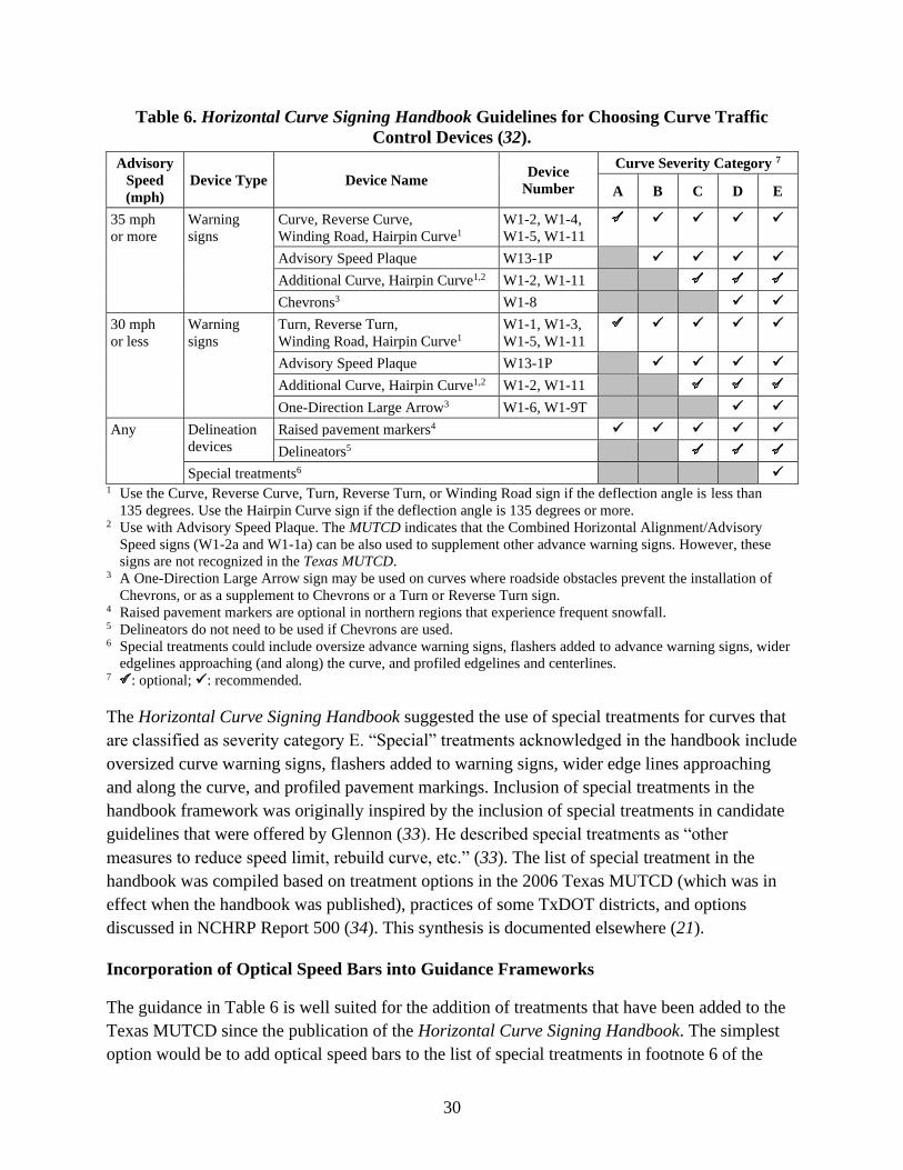
30

Table 6. Horizontal Curve Signing Handbook Guidelines for Choosing Curve Traffic

Control Devices (32).

Advisory

Speed

(mph)

Device Type Device Name Device

Number

Curve Severity Category 7

A B C D E

35 mph

or more

Warning

signs

Curve, Reverse Curve,

Winding Road, Hairpin Curve1

W1-2, W1-4,

W1-5, W1-11

✓ ✓ ✓ ✓

Advisory Speed Plaque W13-1P ✓ ✓ ✓ ✓

Additional Curve, Hairpin Curve1,2 W1-2, W1-11

Chevrons3 W1-8 ✓ ✓

30 mph

or less

Warning

signs

Turn, Reverse Turn,

Winding Road, Hairpin Curve1

W1-1, W1-3,

W1-5, W1-11

✓ ✓ ✓ ✓

Advisory Speed Plaque W13-1P ✓ ✓ ✓ ✓

Additional Curve, Hairpin Curve1,2 W1-2, W1-11

One-Direction Large Arrow3 W1-6, W1-9T ✓ ✓

Any Delineation

devices

Raised pavement markers4 ✓ ✓ ✓ ✓ ✓

Delineators5

Special treatments6 ✓ 1 Use the Curve, Reverse Curve, Turn, Reverse Turn, or Winding Road sign if the deflection angle is less than

135 degrees. Use the Hairpin Curve sign if the deflection angle is 135 degrees or more. 2 Use with Advisory Speed Plaque. The MUTCD indicates that the Combined Horizontal Alignment/Advisory

Speed signs (W1-2a and W1-1a) can be also used to supplement other advance warning signs. However, these

signs are not recognized in the Texas MUTCD. 3 A One-Direction Large Arrow sign may be used on curves where roadside obstacles prevent the installation of

Chevrons, or as a supplement to Chevrons or a Turn or Reverse Turn sign. 4 Raised pavement markers are optional in northern regions that experience frequent snowfall. 5 Delineators do not need to be used if Chevrons are used. 6 Special treatments could include oversize advance warning signs, flashers added to advance warning signs, wider

edgelines approaching (and along) the curve, and profiled edgelines and centerlines. 7 : optional; ✓: recommended.

The Horizontal Curve Signing Handbook suggested the use of special treatments for curves that

are classified as severity category E. “Special” treatments acknowledged in the handbook include

oversized curve warning signs, flashers added to warning signs, wider edge lines approaching

and along the curve, and profiled pavement markings. Inclusion of special treatments in the

handbook framework was originally inspired by the inclusion of special treatments in candidate

guidelines that were offered by Glennon (33). He described special treatments as “other

measures to reduce speed limit, rebuild curve, etc.” (33). The list of special treatment in the

handbook was compiled based on treatment options in the 2006 Texas MUTCD (which was in

effect when the handbook was published), practices of some TxDOT districts, and options

discussed in NCHRP Report 500 (34). This synthesis is documented elsewhere (21).

Incorporation of Optical Speed Bars into Guidance Frameworks

The guidance in Table 6 is well suited for the addition of treatments that have been added to the

Texas MUTCD since the publication of the Horizontal Curve Signing Handbook. The simplest

option would be to add optical speed bars to the list of special treatments in footnote 6 of the

31

table. This option would be consistent with the 2011 Texas MUTCD language regarding optical

speed bars, which calls for their use if other warning devices have been used and found

ineffective.

Optical speed bars could also be incorporated into the existing Texas MUTCD Table 2C-5

(shown as Table 4 in this report) by adding a row to the table. Table 7 shows a candidate revision

to Texas MUTCD Table 2C-5 with a new row added for optical speed bars. This option would

require expanding the scope of the table to include markings in addition to signs. It would also be

desirable to determine how many curves statewide may be “optional” or “recommended” for

optical speed bars based on their posted regulatory speed limits and advisory speeds. In other

words, it would be desirable to determine how many curves have speed differences (regulatory

minus advisory) of 20 mph, 25 mph, or greater. This determination could be made as part of the

ongoing statewide efforts to update curve advisory speeds.

Table 7. Candidate Updated Horizontal Alignment Sign and Marking Selection.

Type of

Horizontal Alignment Sign

Difference between Speed Limit & Advisory Speed

5 mph 10 mph 15 mph 20 mph ≥ 25 mph

Turn (W1-1), Curve (W1-2),

Reverse Turn (W1-3),

Reverse Curve (W1-4),

Winding Road (W1-5), and

Combination Horizontal

Alignment (W1-10 series)

Recommended Required Required Required Required

Advisory Speed Plaque (W13-1P) Recommended Required Required Required Required

Chevrons (W1-8) and/or

One-Direction Large Arrow

(W1-6, W1-9T)

Optional Recommended Required Required Required

Speed Reduction Markings Optional Recommended

33

CHAPTER 4:

TRAFFIC SIGNAL BACKPLATE PRACTICES

According to a joint Institute of Transportation Engineers and FHWA brief on engineering

countermeasures for red-light running published in 2004 (35):

Backplates are used to improve the signal visibility by providing a black

background around the signals, thereby enhancing the contrast. They are

particularly useful for signals oriented in an east-west direction to counteract the

glare effect of the rising and setting sun or areas of visually complex

backgrounds. A retroreflective yellow border strip around the outside perimeter of

signal backplates has been found to significantly reduce night-time crashes at

signals and also helps drivers identify an intersection as signalized during a power

failure.

An FHWA informational guide on signalized intersections published in 2004 (36) contains the

results of two studies that showed safety benefits of backplates. Since then, findings of several

other studies have reinforced the fact that the use of backplates improves safety at signalized

intersections. More recently, FHWA has added backplates with retroreflective borders to the list

of proven low-cost safety countermeasures and published informational brochures and guidelines

for encouraging their use (37, 38).

Over the years, the use of backplates has become more prevalent. However, as a national

standard set forth by the federal MUTCD (1) and adopted by most state departments of

transportation, the use of backplates mostly remains a recommended practice. The Texas

MUTCD mirrors the national standard by including the following statements in Section 4D.12

(2):

• “Guidance: If the posted or statutory speed limit or the 85th-percentile speed on an

approach to a signalized location is 45 mph or higher, signal backplates should be used

on all of the signal faces that face the approach. Signal backplates should also be

considered for use on signal faces on approaches with posted or statutory speed limits or

85th-percentile speeds of less than 45 mph where sun glare, bright sky, and/or complex or

confusing backgrounds indicate a need for enhanced signal face target value.

• Standard: The inside of signal visors (hoods), the entire surface of louvers and fins, and

the front surface of backplates shall have a dull black finish to minimize light reflection

and to increase contrast between the signal indication and its background.

• Option: A yellow retroreflective strip with a minimum width of 1 inch and a maximum

width of 3 inches may be placed along the perimeter of the face of a signal backplate to

project a rectangular appearance at night.”

34

This chapter provides a summary of the literature review conducted to assess experiences of

other states in evaluating and/or adopting the use of signal backplates and any guidelines and/or

standards they may have adopted in the process. The chapter is divided into the following

subsections related to the subject area:

• Case studies showing safety benefits. In general, this section follows a chronological

order.

• Current state of the practice. In this section, states are listed in alphabetical order.

CASE STUDIES

Winston-Salem

A study of black backplates in Winston-Salem, North Carolina (36), found a 32 percent drop in

right-angle collisions at intersections where backplates were installed. However, rear-end crashes

increased after installation of backplates. Overall, there was a 12 percent increase in total

crashes. This increase was attributed to drivers’ sudden braking due to unfamiliarity with such a

treatment.

British Columbia

A British Columbia study (36, 39) involving a comparison of collision frequency analysis before

and after installation of backplates with a 75-mm-wide yellow retroreflective strip around the

outside edge at several intersections concluded that they were effective at reducing the number of

automobile insurance claims by 15 percent. The initial study began in 1998 with six intersections

and was expanded to include several more. A later publication by the same authors (40) reports

the results of a similar before-after safety evaluation of the same treatment at 17 signalized

intersections. Results of this study showed a 15 percent reduction in crash rates. This result

became the basis for the CMF of 0.85 and applies to facilities with 30- to 55-mph posted speeds

with urban and suburban surroundings, some with lighting and some with pedestrian facilities.

A follow-up study evaluated the safety benefits of a combination of visibility improvement (lens

size, new backplates, reflective tape added to existing backplates, and additional signal heads) at

139 intersections (41). The results of this study included:

• Collision reductions of 8.5 percent, 5.9 percent, 6.6 percent, and 7.3 percent for property-

damage-only, daytime, nighttime, and total collisions, respectively.

• Severe collisions showed a nonsignificant reduction of 2.6 percent.

• The reduction in nighttime collisions, for which the improvements are likely to be more

effective, was higher than that of daytime collisions.

35

• Previous studies, which had much lower sample size and were for high-speed roadways,

showed larger benefits, suggesting that safety improvements for high-speed facilities are

higher.

Kentucky

The objective of a Kentucky study was to provide low-cost safety improvement at high-volume

urban intersections and high-speed rural intersections with known red-light running (38, 42).

Thirty signalized intersections with high volumes of crashes were selected throughout Kentucky.

The following two types of retroreflective backplates were installed:

• Black backplates with yellow retroreflective borders.

• Yellow retroreflective backplates.

This evaluation showed the following safety improvements:

• 19.6 percent reduction in total crashes.

• 44.4 percent reduction in angle crashes.

• 10 percent reduction in rear-end crashes.

These benefits exceeded the CMF figure based on the 15 percent reduction previously reported.

Kansas

This limited study included the following two methods to evaluate the effectiveness of

retroreflective signal backplates in reducing red-light running (43):

• Cross-sectional analysis using an intersection with reflective backplates and an

intersection without reflective backplates.

• Before-after study using four intersections.

The cross-sectional analysis found that reflective backplates are effective in reducing red-light

violations in the through and left-turning traffic flows. The before-after study showed a

significant reduction in red-light violations in one of the two treatment sites, according to paired-

t-test statistics.

South Carolina

A 54-month study conducted between 2003 and 2007 examined the application of a 3-inch,

yellow retroreflective border to existing signal backplates at three intersections with high

incidence of crashes (44). The treatment, which was implemented in June 2005, resulted in the

improvements in Table 8.

36

Table 8. Impact of Signal Backplates with Retroreflective Border.

Location Percent Reduction in Crashes/Year

Total Crashes Injury Crashes Late-Night and Early Morning Crashes

1 26.2 31.8 0.6

2 19.7 76.8 85.5

3 38.9 NA 56.5

Average 28.6 36.7 49.6 NA = not applicable

STATE DEPARTMENT OF TRANSPORTATION PRACTICES

Alabama

According to the ALDOT Traffic Signal Design Guide and Timing Manual (45):

• ALDOT suggests that backplates be used on east-west approaches to an intersection.

• Some ALDOT regions/areas require backplates on all approaches, regardless of

orientation, so the region/area traffic engineer should be consulted prior to design.

• While backplates improve signal visibility, they can also become maintenance problems

over time.

• Backplates can crack or tear loose, and increase the wind loading on the signal,

sometimes resulting in increased head sway. For this reason, some region/area traffic

engineers prefer to limit the use of backplates. In some cases, it may be appropriate to use

tethers to stabilize signals heads with backplates against wind loading. Such installations

are subject to approval by ALDOT

Florida

Florida Department of Transportation (FDOT) standard specifications (46) require all signal

heads to have backplates. In addition, the FDOT design manual (47) requires installation of

retroreflective backplate borders on traffic signals for all approaches. FDOT standard

specifications also require signal backplates to meet the following requirements:

• “Provide vehicular traffic signal assemblies as a complete and functioning unit.

Components include, but are not limited to, signal housing, light emitting diode (LED)

signal modules, visors, backplates, and assembly hardware.

• If backplates are mechanically attached, each signal section must have four backplate

mounting attachment points on the back of the signal, on or no more than three inches

from each section corner. Attachment points must be capable of accepting

No. 10-16x3/8-inch or No. 10-24x3/8-inch Type 316 or 304 stainless steel screws for

attaching backplates. Attachment points must not interfere with the operation of traffic

signal section doors.

37

• The housing, doors, visors and backplates must be powder coated dull black (Federal

Standard 595-37038) with a reflectance value not exceeding 25 percent as measured by

ASTM E1347. For plastic heads, the black color must be incorporated into the plastic

material before molding.

• Backplates may be constructed of either aluminum or plastic. Minimum thickness for

aluminum backplates is 0.060 inch and the minimum thickness for plastic backplates is

0.120 inch. The required width of the top, bottom, and sides of backplates must measure

between 5 to 6 inches. Color of backplates must be black. Backplate thickness

measurement must not include the retroreflective sheeting thickness.

• Backplate outside corners must be rounded and all edges must be deburred.

• If louvers are provided, louver orientation must be vertical on sides and horizontal on top

and bottom of the backplate and must be at least 1/2 inch from the inner and outer edge of

the backplate panel. Universal backplates must fit all traffic signals listed on the

Approved Products List.

• Mount the backplate securely to the signal assembly with Type 316 or 304 passivated

stainless-steel installation hardware.

• Backplates, if mechanically attached, must be marked in accordance with 650-2.1, on the

long sides of the backplate.

• Backplates must include retroreflective borders using Type IV yellow retroreflective

sheeting listed on the Approved Products List. Place a 2-inch border on the entire outer

perimeter of the backplate panel, no closer than 1/2 inch from any louvers.

• Install backplates on all vertically mounted plastic signal head assemblies.

• Ensure that the signal housings, backplates, and any other signal assembly components

have a manufacturer’s warranty covering defects for a minimum of three years from the

date of final acceptance. Ensure the warranty includes providing replacements, within

30 calendar days of notification, for defective parts and equipment during the warranty

period at no cost to the Department or the maintaining agency.

• Pedestrian hybrid beacon assembly includes the 3-section signal, hardware, and

backplate.”

Kentucky

According to an FHWA report (38), Kentucky currently does not require retroreflective

backplates; however, when installed, a 2-inch-wide fluorescent yellow reflective tape is to be

applied around the outer perimeter of the face of the backplate. Also, the reflective tape must

comply with the latest ATSM International Standard for Type IX, fluorescent yellow

retroreflective sheeting.

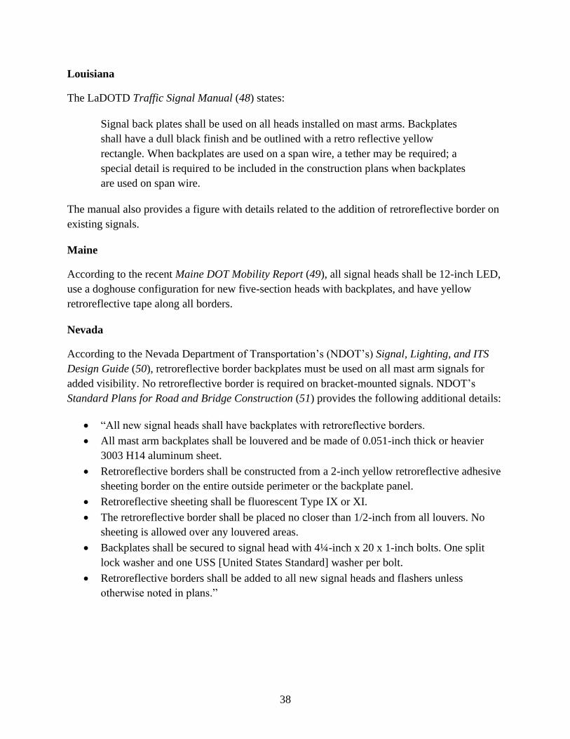
38

Louisiana

The LaDOTD Traffic Signal Manual (48) states:

Signal back plates shall be used on all heads installed on mast arms. Backplates

shall have a dull black finish and be outlined with a retro reflective yellow

rectangle. When backplates are used on a span wire, a tether may be required; a

special detail is required to be included in the construction plans when backplates

are used on span wire.

The manual also provides a figure with details related to the addition of retroreflective border on

existing signals.

Maine

According to the recent Maine DOT Mobility Report (49), all signal heads shall be 12-inch LED,

use a doghouse configuration for new five-section heads with backplates, and have yellow

retroreflective tape along all borders.

Nevada

According to the Nevada Department of Transportation’s (NDOT’s) Signal, Lighting, and ITS

Design Guide (50), retroreflective border backplates must be used on all mast arm signals for

added visibility. No retroreflective border is required on bracket-mounted signals. NDOT’s

Standard Plans for Road and Bridge Construction (51) provides the following additional details:

• “All new signal heads shall have backplates with retroreflective borders.

• All mast arm backplates shall be louvered and be made of 0.051-inch thick or heavier

3003 H14 aluminum sheet.

• Retroreflective borders shall be constructed from a 2-inch yellow retroreflective adhesive

sheeting border on the entire outside perimeter or the backplate panel.

• Retroreflective sheeting shall be fluorescent Type IX or XI.

• The retroreflective border shall be placed no closer than 1/2-inch from all louvers. No

sheeting is allowed over any louvered areas.

• Backplates shall be secured to signal head with 4¼-inch x 20 x 1-inch bolts. One split

lock washer and one USS [United States Standard] washer per bolt.

• Retroreflective borders shall be added to all new signal heads and flashers unless

otherwise noted in plans.”

39

Ohio

The Ohio Department of Transportation’s (ODOT’s) MUTCD does not require signal

backplates, but the ODOT Traffic Engineering Manual (52) states that:

• “For any project using State or Federal funds, louvered reflective backplates are required

for all new signal heads (backplates are required for both mast-arm and span-wire

installations). It is recommended that signal heads be polycarbonate plastic and be

tethered to minimize sway for span-wire type configurations. A signal support analysis

should be performed on all existing strain poles and mast-arm type signal supports to

insure they are structurally adequate for the proposed changes. If span-wire supports are

found deficient for backplates in all directions, then the intersection should be analyzed

for mainline or East/West backplates only. Written documentation and calculations are

required if the proposed additions/changes cannot be implemented.

• Aluminum backplates shall include a fluorescent yellow reflective border.”

Furthermore, Section 732.22 of ODOT’s Construction and Material Specifications (53) requires

backplates meeting the following requirements:

• “Furnish louvered backplates constructed of wrought sheet aluminum, according to

ASTM International B 209 (B 209M), 6061-T6, 0.050-inch minimum thickness. Louvers

shall be at least 8 percent of the total backplate area.

• Backplate base metal shall be anodized to maximize paint adhesion according to

Mil-A-8625, Type II or Type I. Furnish backplates painted on both sides with at least two

coats of flat black alkyd enamel paint or polyester powder coat (no epoxy) closely

matching FED-STD-595b-37038.

• Furnish a backplate that extends 5 inches beyond the outside of the signal assembly on all

sides. The overall outside shape of the installed backplate shall be rectangular. The

backplate shall allow no gaps between the backplate and the signal head or between

signal sections.

• A 2-inch wide continuous outside border of fluorescent yellow reflective sheeting shall

be applied to the front of the backplate. The border shall not be applied over the louvers.

Reflective sheeting shall be Type J, ASTM International D4956 Type XI. Prepare

backplate surfaces in accordance with 630.04 prior to applying the reflective material.

• All assembly and mounting hardware shall be stainless steel conforming to 730.10. If

used, machine nuts shall be thread-deforming or nylon locknuts. Rivets shall not be used

for mounting the backplate to the signal head. A minimum of four mounting points shall

be used on each signal section for attaching the backplate. Furnish all mounting

hardware.”

40

Pennsylvania

The Pennsylvania Department of Transportation issued a strike off letter for standardizing the

use of traffic signal backplates effective July 1, 2017 (54). The decision to standardize was made

at the April 6–7, 2016, District Traffic Engineers Meeting. This letter requires furnishing of

backplates that conform to the following:

• “Shall be one-piece aluminum with a minimum thickness of 0.06 inch (thickness does not

include retroreflective border).

• Shall be powder coated dull black (Federal Standard 595-37038) on both the front and

back sides.

• Top, bottom, and sides shall measure from 5 to 8 inches in width.

• Shall have rounded outside corners.

• Shall include louvers with no louvers closer than 0.5-inch from the inner or 2.5 inches

from the outer edge. Louver orientation shall be vertical on sides and horizontal on top

and bottom.

• Shall provide a minimum of four corner mounting attachment points per section head and

must not interfere with the operation of the section head doors.

• Shall include passivated stainless-steel type 316 or 304 screws, washers, and other

installation hardware required to mount securely.

• Shall be permanently marked on the back side with the manufacturer name, part/model

number and date of manufacturer.

• Universal backplates shall fit all applicable Penn DOT-approved products.

• Shall have a minimum 2-inch fluorescent yellow, Type IX retroreflective border, placed

flush with the outer edge of the backplate and placed no closer than 0.5-inch from all

louvers. No sheeting is allowed over any louvered area.”

All signal heads and backplates mounted on temporary traffic control signals on pedestal-

mounted portable traffic control signal systems are also required to meet these specifications.

This standard also states that “traffic signal backplates shall be one-piece aluminum, black,

between 5 and 8 inches, and include yellow retroreflective tape around the edges.”

Virginia

In April 2018, the Virginia Department of Transportation (VDOT) issued an Instructional and

Informational Memorandum (55) to update the 2011 VDOT MUTCD Revision 1 to address

high-visibility signal backplates. Key points are as follows:

• “Option 20b: High visibility signal backplates may be used on traffic control signals.

• Standard 20c: If used, high visibility signal backplates shall consist of a 3-inch wide

fluorescent yellow retroreflective strip along the outermost perimeter of the front face of

a signal backplate.

41

• Support 20d: If used, it is desirable to install high visibility signal backplates on every

signal face at the intersection.

• Standard 20e: If used on an approach, high visibility signal backplates shall be used on all

signal faces facing that approach.

• Option 20f: High visibility signal backplates may be used on signal faces at an individual

intersection and not at an adjacent intersection(s) along a corridor.

• Standard 20g: Except as provided in Paragraph 20i, high visibility signal backplates shall

be used on signal faces at signalized intersections with at least one approach that has one

or more of the following characteristics:

A. High speed roadway—where the posted or statutory speed limit or the

85th-percentile speed on an approach is 45 mph or greater;

B. Corridor of Statewide Significance (Costs);

C. Principal arterial;

D. Intersections with limited sight distances to the signal face, per Table 4D.12 in this

Supplement; or

E. Intersection at interchange and/or freeway ramp terminals.

• Guidance 20h: Except as provided in Paragraph 20i, high visibility signal backplates

should be used on signal faces at signalized intersections with at least one approach that

has one or more of the following characteristics:

A. Where visual roadside clutter or the natural or manmade surroundings would

distract road users’ attention from the traffic control signal;

B. Where crash history (angle, rear end, or other) or known red light running could be

correctable by the installation of high visibility signal backplates;

C. Is located in an area with known or frequent power outages, especially at locations

without an Uninterruptible Power Supply (UPS); or

D. A location that is the first signal encountered after a long section of roadway

without traffic control signals.

• Option 20i: Once an intersection or approach has been identified for high visibility signal

backplate use, high visibility signal backplates may be omitted on any intersection

approach that has one or more of the following characteristics:

A. Streetscape corridor or location with decorative traffic signal poles;

B. Skewed angles where high visibility signal backplates could inadvertently provide

unwanted visibility for the wrong approach;

C. Low-volume approach, such as a low-volume commercial entrance or private

entrance (see Road Design Manual Appendix F for definitions), or secondary

roadway; or

D. Any or all approaches where engineering judgment determines that high visibility

signal backplates are inappropriate.

• Standard 21: Except as provided in Paragraphs 20b and 20c, the inside of signal visors

(hoods), the entire surface of louvers and fins, and the front surface of backplates shall

42

have a dull black finish to minimize light reflection and to increase contrast between the

signal indication and its background.

• Temporary Traffic Control Signals (Section 4D.32) Option: High visibility signal

backplates (see Section 4D.12 in this Supplement) may be used on temporary and

portable traffic control signals.

• Freeway Ramp Control Signals Standard: High visibility signal backplates shall not be

used on freeway entrance ramp control signals.

• Flashing Beacons

o 4L.01 Standard: Except as provided in Section 4L.02 in this Supplement, high

visibility signal backplates shall not be used on flashing beacons.

o 4L.02 Option: High visibility signal backplates may be used on intersection control

beacons based on the provisions in Section 4D.12 in this Supplement.”

Washington

The Washington State Department of Transportation design manual (56) requires the use of

backplates for all overhead-mounted displays for new, updated, or rebuilt signal faces. The

manual also requires a minimum 16.5-ft clearance over the roadway with a backplate installed.

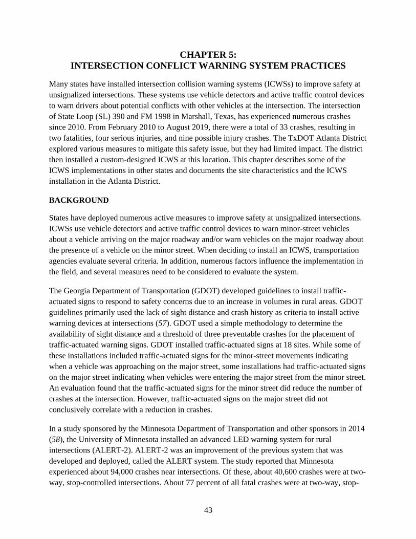
43

CHAPTER 5:

INTERSECTION CONFLICT WARNING SYSTEM PRACTICES

Many states have installed intersection collision warning systems (ICWSs) to improve safety at

unsignalized intersections. These systems use vehicle detectors and active traffic control devices

to warn drivers about potential conflicts with other vehicles at the intersection. The intersection

of State Loop (SL) 390 and FM 1998 in Marshall, Texas, has experienced numerous crashes

since 2010. From February 2010 to August 2019, there were a total of 33 crashes, resulting in

two fatalities, four serious injuries, and nine possible injury crashes. The TxDOT Atlanta District

explored various measures to mitigate this safety issue, but they had limited impact. The district

then installed a custom-designed ICWS at this location. This chapter describes some of the

ICWS implementations in other states and documents the site characteristics and the ICWS

installation in the Atlanta District.

BACKGROUND

States have deployed numerous active measures to improve safety at unsignalized intersections.

ICWSs use vehicle detectors and active traffic control devices to warn minor-street vehicles

about a vehicle arriving on the major roadway and/or warn vehicles on the major roadway about

the presence of a vehicle on the minor street. When deciding to install an ICWS, transportation

agencies evaluate several criteria. In addition, numerous factors influence the implementation in

the field, and several measures need to be considered to evaluate the system.

The Georgia Department of Transportation (GDOT) developed guidelines to install traffic-

actuated signs to respond to safety concerns due to an increase in volumes in rural areas. GDOT

guidelines primarily used the lack of sight distance and crash history as criteria to install active

warning devices at intersections (57). GDOT used a simple methodology to determine the

availability of sight distance and a threshold of three preventable crashes for the placement of

traffic-actuated warning signs. GDOT installed traffic-actuated signs at 18 sites. While some of

these installations included traffic-actuated signs for the minor-street movements indicating

when a vehicle was approaching on the major street, some installations had traffic-actuated signs

on the major street indicating when vehicles were entering the major street from the minor street.

An evaluation found that the traffic-actuated signs for the minor street did reduce the number of

crashes at the intersection. However, traffic-actuated signs on the major street did not

conclusively correlate with a reduction in crashes.

In a study sponsored by the Minnesota Department of Transportation and other sponsors in 2014

(58), the University of Minnesota installed an advanced LED warning system for rural

intersections (ALERT-2). ALERT-2 was an improvement of the previous system that was

developed and deployed, called the ALERT system. The study reported that Minnesota

experienced about 94,000 crashes near intersections. Of these, about 40,600 crashes were at two-

way, stop-controlled intersections. About 77 percent of all fatal crashes were at two-way, stop-

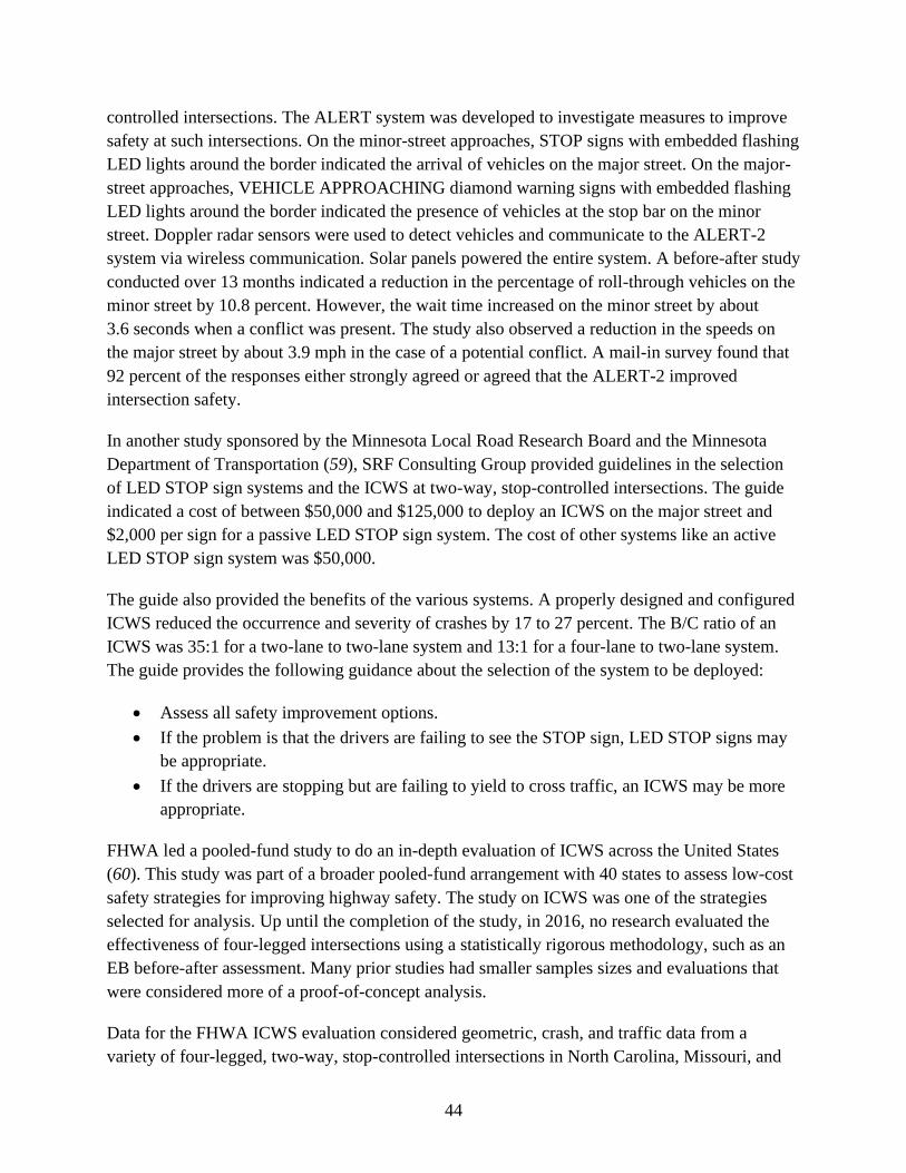
44

controlled intersections. The ALERT system was developed to investigate measures to improve

safety at such intersections. On the minor-street approaches, STOP signs with embedded flashing

LED lights around the border indicated the arrival of vehicles on the major street. On the major-

street approaches, VEHICLE APPROACHING diamond warning signs with embedded flashing

LED lights around the border indicated the presence of vehicles at the stop bar on the minor

street. Doppler radar sensors were used to detect vehicles and communicate to the ALERT-2

system via wireless communication. Solar panels powered the entire system. A before-after study

conducted over 13 months indicated a reduction in the percentage of roll-through vehicles on the

minor street by 10.8 percent. However, the wait time increased on the minor street by about

3.6 seconds when a conflict was present. The study also observed a reduction in the speeds on

the major street by about 3.9 mph in the case of a potential conflict. A mail-in survey found that

92 percent of the responses either strongly agreed or agreed that the ALERT-2 improved

intersection safety.

In another study sponsored by the Minnesota Local Road Research Board and the Minnesota

Department of Transportation (59), SRF Consulting Group provided guidelines in the selection

of LED STOP sign systems and the ICWS at two-way, stop-controlled intersections. The guide

indicated a cost of between $50,000 and $125,000 to deploy an ICWS on the major street and

$2,000 per sign for a passive LED STOP sign system. The cost of other systems like an active

LED STOP sign system was $50,000.

The guide also provided the benefits of the various systems. A properly designed and configured

ICWS reduced the occurrence and severity of crashes by 17 to 27 percent. The B/C ratio of an

ICWS was 35:1 for a two-lane to two-lane system and 13:1 for a four-lane to two-lane system.

The guide provides the following guidance about the selection of the system to be deployed:

• Assess all safety improvement options.

• If the problem is that the drivers are failing to see the STOP sign, LED STOP signs may

be appropriate.

• If the drivers are stopping but are failing to yield to cross traffic, an ICWS may be more

appropriate.

FHWA led a pooled-fund study to do an in-depth evaluation of ICWS across the United States

(60). This study was part of a broader pooled-fund arrangement with 40 states to assess low-cost

safety strategies for improving highway safety. The study on ICWS was one of the strategies

selected for analysis. Up until the completion of the study, in 2016, no research evaluated the

effectiveness of four-legged intersections using a statistically rigorous methodology, such as an

EB before-after assessment. Many prior studies had smaller samples sizes and evaluations that

were considered more of a proof-of-concept analysis.

Data for the FHWA ICWS evaluation considered geometric, crash, and traffic data from a

variety of four-legged, two-way, stop-controlled intersections in North Carolina, Missouri, and

45

Minnesota (all data collected from the respective state agency). A total of 93 intersections were

considered for the study. Data from Minnesota consisted of 10 two-lane at two-lane intersections

and three four-lane at two-lane intersections. Data from Missouri consisted of six two-lane at

two-lane intersections and eight four-lane at two-lane intersections. Data from North Carolina

consisted of 53 two-lane at two-lane intersections and 13 four-lane at two-lane intersections.

The FHWA study objective and methodology were to measure effectiveness as represented by

crash frequency, while controlling for other design and environmental factors. The types of crash

variables included total crashes, injury crashes (e.g., fatal, incapacitating, non-incapacitating, and

injury), right-angle crashes, rear-end crashes, and nighttime crashes. The other design and

environmental factors included installation type (e.g., ICWS combination), location (e.g., post

mounted versus overhead), number of approaches, traffic volume, posted speed limit, presence of

turn lanes, intersection lighting, and crash frequency during the before analysis period.

Overall, the FHWA study results indicated that all crash types have reductions for both four-lane

at two-lane intersections and two-lane at two-lane intersections. Table 9 shows the CMFs for

total, fatal and injury, right-angle, rear-end, and nighttime crashes as measured from the research.

For two-lane at two-lane intersections, the study found statistically significant crash reductions at

the 95 percent confidence level for all crash types except nighttime crashes. For four-lane at two-

lane intersections, the study found statistical significance at the 95-percent confidence level for

all crash types except rear-end crashes. Some of the rationale for why statistical significance

could not be achieved was the relatively small sample sizes for some crash types. The most

significant crash reductions occurred for nighttime crashes at four-lane at two-lane intersections.

Table 9. Crash Modification Factors from the FHWA ICWS Evaluation.

Crash Type Two-Lane at Two-Lane

Intersections

Four-Lane at Two-Lane

Intersections

Total 0.733* 0.827*

Fatal and injury 0.701* 0.802*

Right angle 0.803* 0.850*

Rear end 0.425* 0.973

Nighttime 0.898 0.612* * Statistical significance at the 95 percent confidence interval.

Using the data from North Carolina, the research team performed a disaggregated analysis to

identify specific conditions where ICWS installation was more effective. The analysis considered

specific installation types, such as the use of overhead signs versus post-mounted signs and the

integration of flashers. Overall, the research team found larger crash reductions for ICWS

installed on the major approach with post-mounted signs for two-lane at two-lane intersections.

For four-lane at two-lane intersections, the research team found no major differences between

placements on the major versus minor approaches. However, a larger crash reduction did occur

for intersections with overhead lighting.

46

The FHWA research also included a basic estimation of economic costs that included actual

construction, implementation, and maintenance costs. Table 10 shows a summary of the average

costs (in 2014 dollars) by intersection type for all three states. The values shown consider the

different installation type variations, with placement of ICWS on multiple approaches and the

presence of a four-lane highway as more costly conditions. Additionally, some states may have

different arrangements for managing and handling communications, whether wired or wireless.

Various communication systems can also influence cost considerations.

Table 10. Average Cost Estimates by Intersection Type (in 2014 Dollars).

Intersection Type Installation Annual Maintenance and Operations

Two-lane at two-lane $41,590 $1,075

Four-lane at two-lane $106,150 $1,200 ($3,400 wireless)

The FHWA research team found the ICWS was relatively economical when estimating B/C

ratios. The study cited a B/C ratio of 27:1 for all two-lane at two-lane intersections and 10:1 for

four-lane at two-lane intersections, given conservative cost and service life assumptions while

only factoring the benefits for total crashes. The research team used an average service of

10 years for each intersection. The benefit estimation used an FHWA mean comprehensive crash

cost estimate of $9.2 million (in 2014 dollars) for the statistical value of a human life. The

research team also used an estimated average annual avoidance of 0.95 crashes per intersection

for two-lane at two-lane intersections and 0.79 crashes per intersection for four-lane at two-lane

intersections.

The FHWA research report reflects practices used up until the 2016 publication date. More

recent advancements in wireless detection and communication systems may have an influence on

effectiveness. Additionally, the study did not consider the use of advance warning systems for

overhead ICWS on major routes. The report authors also note that the ICWS installations

evaluated did not consider the use of blank-out signs. Specifically, a survey found that 28 percent

of participants felt that inactive signs lessened the need to check for cross traffic. The study

authors recommended that drivers’ misinterpretations of static signs in the event of power failure

or sensor malfunction be addressed with education and outreach.

ATLANTA DISTRICT SITE CHARACTERISTICS

The intersection of SL 390 (major street) and FM 1998 (minor street) is east of the city of

Marshall. This intersection is characterized by a slight skew. SL 390 is a north-south arterial with

a horizontal curve on the northbound approach (see Figure 23). In addition, all approaches to the

intersection are high speed (i.e., a 65-mph speed limit on SL 390 and a 60-mph speed limit on

FM 1998) (see Figure 24). On the FM 1998 westbound and eastbound approaches, sight distance

restrictions limit the visibility of the major street traffic (see Figure 25 and Figure 26,

respectively).

47

Figure 23. ICWS Installation Site in Marshall, Texas


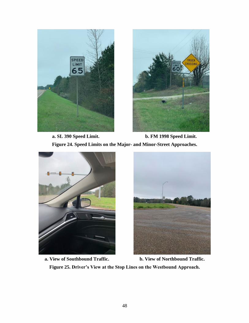
48

a. SL 390 Speed Limit. b. FM 1998 Speed Limit.

Figure 24. Speed Limits on the Major- and Minor-Street Approaches.

a. View of Southbound Traffic. b. View of Northbound Traffic.

Figure 25. Driver’s View at the Stop Lines on the Westbound Approach.

49

a. View of Southbound Traffic. b. View of Northbound Traffic.

Figure 26. Drivers at the Stop Lines on the Eastbound Approach.

Before the implementation of the ICWS, the minor street included two sets of transverse rumble

strips, STOP AHEAD pavement markings, and Stop Ahead signs (W3-1) on the approaches (see

Figure 27); and STOP pavement markings, STOP signs, and two overhead stop beacons at the

intersection (see Figure 28). Each overhead stop beacon consisted of two signal sections with a

flashing circular red signal indication in each signal section. The major-street approaches

included two overhead warning beacons at the intersection (see Figure 29). Each overhead

warning beacon consisted of two signal sections with a flashing circular yellow signal indication

in each signal section. All the overhead beacons were installed on span wire with luminaire

lighting on the two strain poles at the intersection.

50

a. Transverse Rumble Strips and Stop

Ahead Sign.

b. STOP AHEAD Pavement Markings.

Figure 27. Example of Treatments on the Minor-Street Approaches.

Figure 28. Minor-Street Approach before ICWS


51

Figure 29. Major-Street Approach before ICWS


ATLANTA DISTRICT ICWS

To improve safety at the intersection, the Atlanta District implemented an ICWS in December

2019. The TxDOT Atlanta District plans to collect crash data and conduct a before-after study to

evaluate the effectiveness of the ICWS installed in Marshall.

Intersection Improvements

At the intersection, the district installed overhead flashing beacon assemblies on mast arms on all

four approaches. The overhead flashing beacons were moved from span wire to mast arms to

improve their visibility. Three flashing warning beacons were installed on the SL 390 (major-

street) approaches (see Figure 30), and two flashing stop beacons were installed on the FM 1998

(minor-street) approaches (see Figure 31). The district also improved lighting by installing

luminaires on all four signal poles at the intersection and an additional two luminaires on the

major-street approaches to the intersection. A supplemental plaque (CROSS STREET DOES

NOT STOP) was also installed on each of the STOP signs on the minor street.

52

Figure 30. Intersection Improvements on SL 390.

Figure 31. Intersection Improvements on FM 1998.

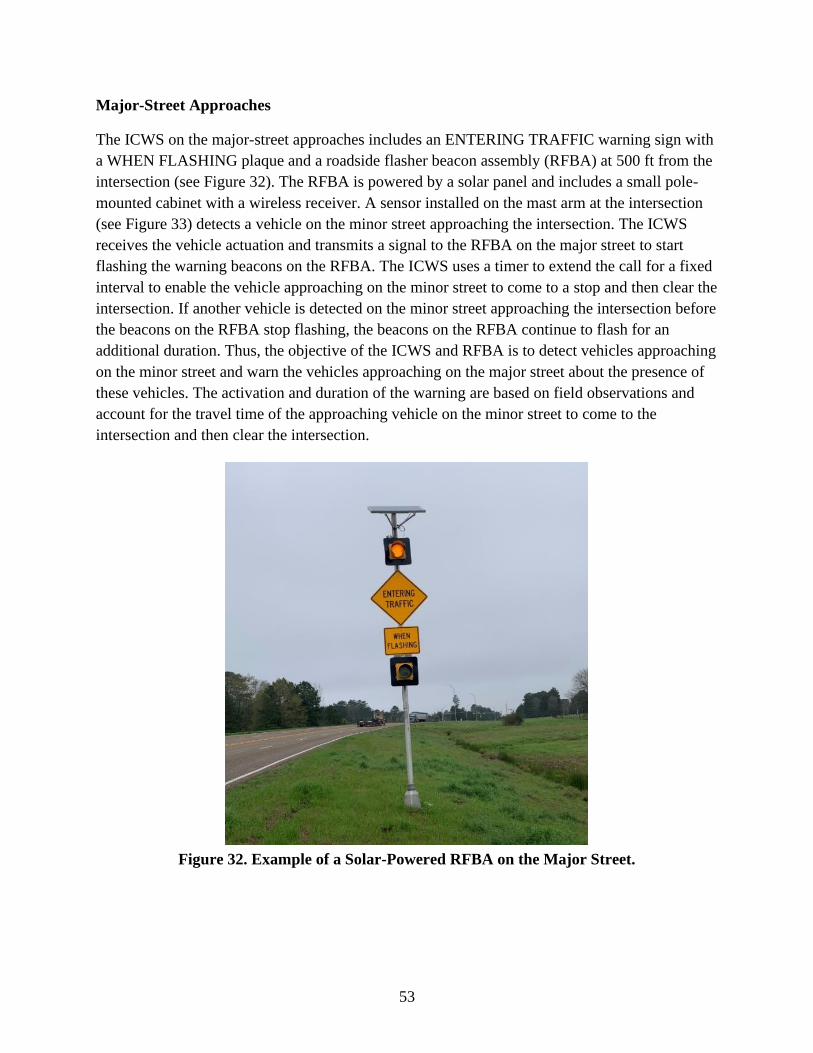
53

Major-Street Approaches

The ICWS on the major-street approaches includes an ENTERING TRAFFIC warning sign with

a WHEN FLASHING plaque and a roadside flasher beacon assembly (RFBA) at 500 ft from the

intersection (see Figure 32). The RFBA is powered by a solar panel and includes a small pole-

mounted cabinet with a wireless receiver. A sensor installed on the mast arm at the intersection

(see Figure 33) detects a vehicle on the minor street approaching the intersection. The ICWS

receives the vehicle actuation and transmits a signal to the RFBA on the major street to start

flashing the warning beacons on the RFBA. The ICWS uses a timer to extend the call for a fixed

interval to enable the vehicle approaching on the minor street to come to a stop and then clear the

intersection. If another vehicle is detected on the minor street approaching the intersection before

the beacons on the RFBA stop flashing, the beacons on the RFBA continue to flash for an

additional duration. Thus, the objective of the ICWS and RFBA is to detect vehicles approaching

on the minor street and warn the vehicles approaching on the major street about the presence of

these vehicles. The activation and duration of the warning are based on field observations and

account for the travel time of the approaching vehicle on the minor street to come to the

intersection and then clear the intersection.

Figure 32. Example of a Solar-Powered RFBA on the Major Street.

54

a. Mast Arm with Sensor. b. Sensor Installed on Mast Arm.

Figure 33. Example of a Sensor to Detect Vehicles Approaching on the Minor Street.

Minor-Street Approaches

On the minor-street approaches, the ICWS includes a diamond-shaped, LED blank-out sign with

a static WHEN FLASHING plaque and two flashing warning beacons (see Figure 34). This sign

assembly is located on the opposite side of the intersection from approaching minor-street traffic.

A sensor installed on the RFBA (see Figure 35) detects vehicles approaching the intersection on

the major street and sends the actuation via a radio signal to the ICWS. The ICWS then activates

the blank-out sign (i.e., displays TRAFFIC APPROACHING) and beacons to warn the

approaching minor-street vehicles (see Figure 36). The ICWS uses a delay timer to ensure that

the warning beacons flash and the sign displays the TRAFFIC APPROACHING message until

the major-street vehicle passes through the intersection. The delay timer is based on the travel

time from the RFBA to the intersection and was calibrated based on field observations.

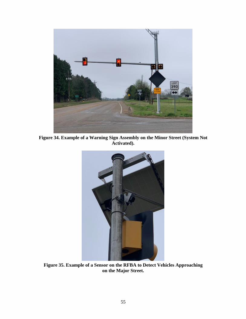
55

Figure 34. Example of a Warning Sign Assembly on the Minor Street (System Not

Activated).

Figure 35. Example of a Sensor on the RFBA to Detect Vehicles Approaching

on the Major Street.

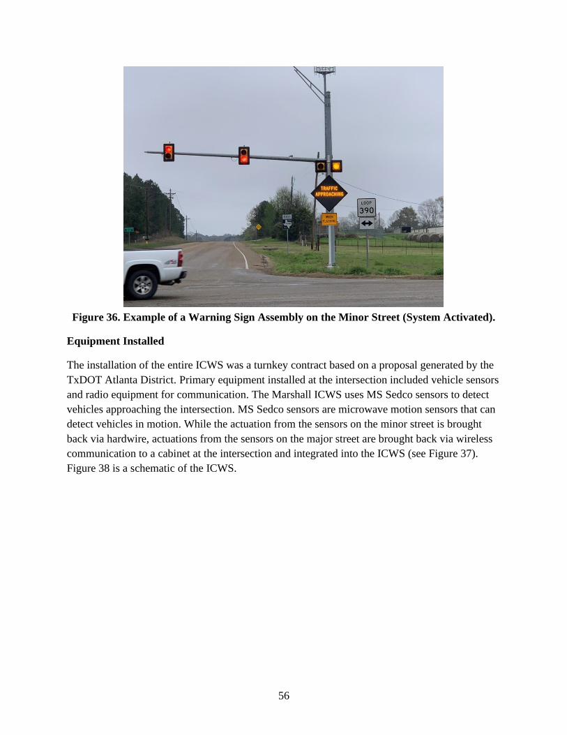
56

Figure 36. Example of a Warning Sign Assembly on the Minor Street (System Activated).

Equipment Installed

The installation of the entire ICWS was a turnkey contract based on a proposal generated by the

TxDOT Atlanta District. Primary equipment installed at the intersection included vehicle sensors

and radio equipment for communication. The Marshall ICWS uses MS Sedco sensors to detect

vehicles approaching the intersection. MS Sedco sensors are microwave motion sensors that can

detect vehicles in motion. While the actuation from the sensors on the minor street is brought

back via hardwire, actuations from the sensors on the major street are brought back via wireless

communication to a cabinet at the intersection and integrated into the ICWS (see Figure 37).

Figure 38 is a schematic of the ICWS.

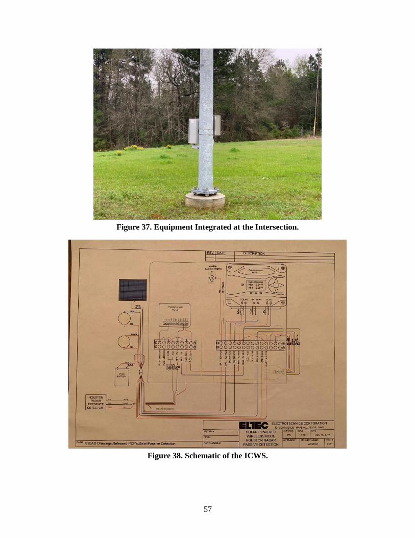
57

Figure 37. Equipment Integrated at the Intersection.

Figure 38. Schematic of the ICWS.

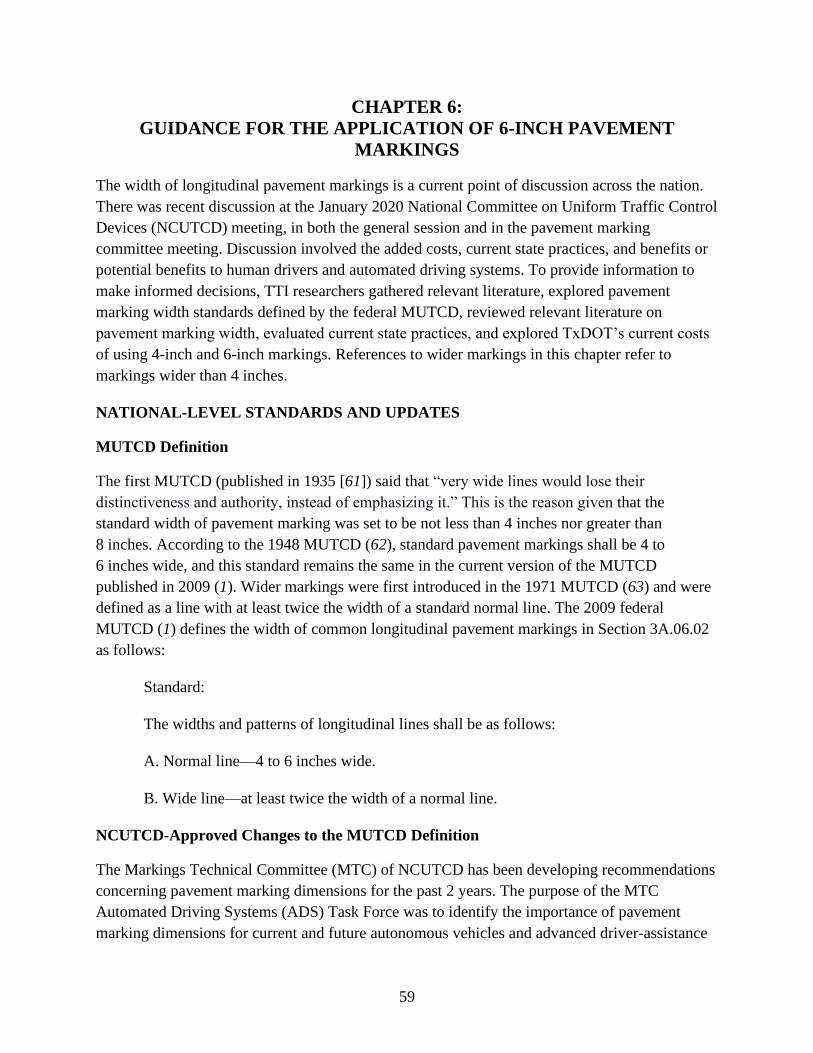
59

CHAPTER 6:

GUIDANCE FOR THE APPLICATION OF 6-INCH PAVEMENT

MARKINGS

The width of longitudinal pavement markings is a current point of discussion across the nation.

There was recent discussion at the January 2020 National Committee on Uniform Traffic Control

Devices (NCUTCD) meeting, in both the general session and in the pavement marking

committee meeting. Discussion involved the added costs, current state practices, and benefits or

potential benefits to human drivers and automated driving systems. To provide information to

make informed decisions, TTI researchers gathered relevant literature, explored pavement

marking width standards defined by the federal MUTCD, reviewed relevant literature on

pavement marking width, evaluated current state practices, and explored TxDOT’s current costs

of using 4-inch and 6-inch markings. References to wider markings in this chapter refer to

markings wider than 4 inches.

NATIONAL-LEVEL STANDARDS AND UPDATES

MUTCD Definition

The first MUTCD (published in 1935 [61]) said that “very wide lines would lose their

distinctiveness and authority, instead of emphasizing it.” This is the reason given that the

standard width of pavement marking was set to be not less than 4 inches nor greater than

8 inches. According to the 1948 MUTCD (62), standard pavement markings shall be 4 to

6 inches wide, and this standard remains the same in the current version of the MUTCD

published in 2009 (1). Wider markings were first introduced in the 1971 MUTCD (63) and were

defined as a line with at least twice the width of a standard normal line. The 2009 federal

MUTCD (1) defines the width of common longitudinal pavement markings in Section 3A.06.02

as follows:

Standard:

The widths and patterns of longitudinal lines shall be as follows:

A. Normal line—4 to 6 inches wide.

B. Wide line—at least twice the width of a normal line.

NCUTCD-Approved Changes to the MUTCD Definition

The Markings Technical Committee (MTC) of NCUTCD has been developing recommendations

concerning pavement marking dimensions for the past 2 years. The purpose of the MTC

Automated Driving Systems (ADS) Task Force was to identify the importance of pavement

marking dimensions for current and future autonomous vehicles and advanced driver-assistance

60

systems (ADAS). The ADS Task Force reviewed existing literature and met with manufacturers

and industry representatives to get more information on how pavement marking dimensions

impact their systems. The task force’s goal was to provide recommendations to MTC to update

Part 3 of the MUTCD with revised guidelines and standards to make improvements for ADS.

The discussion also noted the marking improvements for ADS would also provide benefits to

human drivers. After several reviews and revisions, some of the proposed recommendations were

approved by the NCUTCD Council in January 2020 (64). Since FHWA can only revise the

MUTCD through the federal rulemaking process, the proposal was submitted to FHWA for

consideration to include in the next edition of the MUTCD. FHWA can choose to fully

implement, partially implement, or ignore the proposed changes.

In summary, NCUTCD recommendations, as they pertain to markings, were to install more

pavement marking material on the road. NCUTCD recommended using 6-inch-wide normal

markings on all interstate, freeway, expressway, and corresponding ramp interchanges. Also,

6-inch-wide edge lines should be placed on all other roads with speeds of 55 mph or more and an

average daily traffic (ADT) of 6000 vehicles per day (vpd) or greater. Otherwise, a normal

marking shall be 4 to 6 inches wide. Furthermore, the width of wider lines shall be 8 inches or

more when used with a 4-inch normal line and 10 inches or more when used with a 6-inch

normal line. The original proposal did not have the volume criteria and was for all roads 45 mph

or above. The volume criterion was added to reduce costs due to the mileage of low-volume

roads and to not dissuade the usage of markings where they were not warranted by the MUTCD.

The speed threshold was increased to again reduce the number of roads impacted and the

associated costs. The recommendations do not address lane line pavement markings on multilane

divided or undivided facilities that are excluded from the interstate, freeway, and expressway

categories. This appears to be a gap in the recommendations that would pertain to Texas

highways.

In addition to the increased use of 6-inch-wide markings, NCUTCD also recommended guidance

on broken lane line markings and a standard for dotted lines. The recommendation for the broken

lane lines was to change the marking-to-gap ratio to increase the length of the marking and

reduce the length of the gap. The current marking-to-gap ratio is a 10-foot marking and 30-foot

gap for a 40-foot cycle length. The guidance was to have a 15-foot marking with a 25-foot gap

and keeping the 40-foot cycle length. The guidance was specific to interstates, freeways, and

expressways. The dotted line recommendations were to require dotted lane line and dotted line

extensions across all exit lanes.

PAST RESEARCH ON PAVEMENT MARKING WIDTH

This section summarizes relevant research on the impacts of wider pavement markings in three

areas: vehicle operations, safety, and visibility.

61

Impact of Wider Markings on Vehicle Operations

TTI researchers were unable to find any field studies that evaluated the impact of marking width

on speed or lane position on multilane facilities. However, several operational-based studies

discovered that wider pavement markings generally have minimal impacts on vehicle speed or

lane position on two-lane, two-way highways (65, 66, 67, 68, 69, 70, 71). A driving simulation

study observed the effect of 4-inch versus 6-inch edge line markings at four different levels of

deterioration (0 percent, 25 percent, 50 percent, and 75 percent) during daytime and nighttime

conditions (65). The result did not show any noticeable effect of the 6-inch-wide edge lines at the

0 percent, 25 percent, and 50 percent deterioration levels. Statistically, reliable lane deviation

was found only at the 75 percent deterioration level—0.54 ft and 0.61 ft for 6-inch and 4-inch

edge lines, respectively. This result indicates that the effect of marking width on lane deviation

was not significant until the markings were worn to a 75 percent level, in which case the 6-inch

marking resulted in a lower lane deviation than the 4-inch marking. The results may be limited

due to the nature of simulator studies and their inability to perfectly replicate an actual driving

environment. A simulator study by McKnight et al. (66) showed a decline in lane-keeping

performance with the decrease in pavement marking width while driving over rain-covered

surfaces at night. Researchers concluded that under such conditions, 6- and 8-inch lane lines

allow for better lane keeping than 4-inch lines. McKnight et al. also found that for other

conditions, except for when contrast is extremely low, variation in marking width appeared to

have no influence on lane keeping. A driving simulator study conducted in New Zealand

revealed that drivers choose a slower speed when driving with wide center line markings due to

the higher risk perception (67). However, this study did not clearly reveal the width of markings

used.

An interview of 18 driving instructors revealed that 16 of them preferred 8-inch edge lines while

driving because it helped them to stay in their respective lane (68). However, on-road

investigations comparing pavement marking width found no statistically significant changes in

vehicle speed, encroachments (center line and edge line), and lateral position while comparing

4-inch markings with 6-inch markings (69) or 8-inch markings (70, 71). All markings analyzed

in these three studies were installed on rural two-lane, two-way undivided highways (with and

without horizontal curves). A closed-course human factors study found that the width of

pavement markings had a larger impact than the brightness of pavement markings on lateral

placement, edge line encroachments, and driver eye glance patterns (72). Because previous

studies showed inconsistent results, researchers have suggested a thorough statistical analysis

using multivariate techniques to understand the widening impact of pavement markings on

vehicle operations. An ongoing TTI study sponsored by the Minnesota Department of

Transportation (73) is evaluating the impacts of marking width, lane line cycle pattern, and

contrast pavement markings on driver behavior. This study is expected to be completed in 2021.

A recent study explored the impact of wider markings on the functionality of ADAS (74). The

results found some improvement in the lane departure warning/lane-keeping assistance lane

62

tracking confidence when wider 6-inch markings were present compared to 4-inch markings.

This means the system would function as it is supposed to a higher percentage of the time

because it was able to track the marking more efficiently. The researchers indicated that the

wider markings may have their biggest benefit for ADAS, and likely for human drivers as well,

when the viewing conditions are more difficult. These viewing conditions include wet and rainy

conditions, glare conditions, and when the markings are faded and less reflective than when new.

Impact of Wider Markings on Safety

An evaluation of safety studies resulted in findings that generally show a positive safety

relationship with the increasing width of pavement markings (65, 69, 75, 76, 77, 78, 79, 80).

Table 11 summarizes the crash reductions identified in the literature when studies compared the

safety effect of 4-inch markings with 5-inch or 6-inch markings.

Table 11 indicates that some studies found statistically significant reduction in crashes (65, 69,

75, 76, 77), whereas some studies did not find any statistically significant changes in crashes due

to wider markings (78, 79, 80). Even when statistically significant reductions were not found, it

was generally the case that some level of crash reduction occurred. Increases in crashes were a

rarity in the literature. It is suspected that limited data availability and lack of experimental

control are limitations to these crash investigations that result in the range of significant and non-

significant findings.

Carlson and Wagner (81) performed a B/C analysis of wider edge lines on rural, two-lane

highways using fatal and injury crashes from Kansas data. The result showed a strong B/C ratio

for both fatal and injury crashes. Every $1 investment in wider edge lines results in a $21.72–

$43.96 return in fatal crashes and a $11.16–$11.24 return in injury crashes and their related

costs. Potts et al. (77) found a range of crash reductions when evaluating the Missouri

Department of Transportation (MoDOT) Smooth Roads Initiative (SRI). This initiative focused

on improving rideability and visibility along MoDOT roads. The initiative implemented

combinations of wider markings, rumble strips, and roadway resurfacing. Statistically significant

crash reductions were found for many combinations of treatments and roadway types. When the

treatment was only wider markings with and without resurfacing, statistically significant crash

reductions ranged from 9 to 46 percent. In some cases, insignificant reductions, and even some

increases in certain crash types, were found. The researchers attributed the increases to factors

outside the influence of the SRI. B/C analyses were performed on the data and found a range

between 5.7 and over 100.

63

Table 11. Summary of the Impact of Wider Pavement Markings on Safety.

Location Methodology Data Result Ref.

Idaho (rural

two-lane

highways)

EB before-after

analysis

Before period: 5 years of crash

data from 2010 to 2014

(i.e., when edge line width was

4 inches)

After period: 2016 crash data


6 inches)

Total crashes: 17 percent

reduction

Fatal and severe injury

crashes: 14 percent reduction.

Also, at 90 percent confidence

interval, total crash rate

reduced by 5.5 percent; at

95 percent confidence interval,

fatal and severe injury crash

rate reduced by 12.6 percent.

65

Illinois (rural

two-lane

highways)

Negative

binomial

regression

5 years of crash data from 2001

to 2006 with 4-inch edge and

center lines compared to 5-inch

edge and center lines

Total crashes significantly

decreased with an increase in

edge line width

69

Michigan (rural

two-lane

highways)

EB method of

before-after

analysis




4 inches)

After period: 2 years of crash



6 inches)

At a 95 percent confidence

interval, total crashes reduced

by 7.1 percent because of

installing 6-inch-wide edge

lines

69

Minnesota

(undivided,

rural, two-lane,

two-way

highways)

Cross

comparison

Crash data of 2 years before and

after 6-inch edge line installation

during 2010 and 2011

Total crashes: 15.7 percent

reduction

Severe crashes: 10.4 percent

reduction

Run-off-the-road (ROR)

crashes: 34.2 percent

reduction

Severe ROR crashes:

85.7 percent reduction

75

Kansas (rural

two-lane

highways)

EB method of

before-after

analysis




4 inches)




6 inches)

At 95 percent confidence




lines

76

Michigan (rural

two-lane

highways;

multilane

divided

highways)

Generalized

linear segmented

regression

analysis



(i.e., when edge line width

was 4 inches)




6 inches)





lines. No statistically

significant reduction was

found for multilane highways.

76

64

Location Methodology Data Result Ref.

Illinois (rural

two-lane

highways;

multilane

divided

highways)

Negative

binomial

regression

5 years of crash data from 2001

to 2006 with 4-inch markings

compared to 5-inch markings





lines. No statistically

significant reduction was

found for multilane highways.

76

Missouri (rural

multilane

facilities; rural

two-lane

highways)

EB method of

before-after

analysis



(i.e., when lane line and edge line

width was 4 inches)

After period: 1 year of crash

data from 2007 (i.e., when lane

line and edge line width was

6 inches)

Rural multilane facilities had

statistically significant 9 to

46 percent reduction in fatal

and injury crashes. Rural two-

lane highways showed crash

reductions but not statistically

significant.

77

Alabama,

Maine,

Massachusetts,

New Mexico,

Ohio, South

Dakota, and

Texas (rural

two-lane

highways)

Cross

comparison

Compared crash data for 8-inch

versus 4-inch edge lines

No reduction in crashes (for

roads 5000–10,000 AADT)

78

New Mexico

(rural two-lane

highways)

Before-after

analysis




width was 4 inches or no edge

line)




width was 8 inches)

Did not have a significant

effect on mitigating ROR

crashes (10 percent reduction

in treatment location and

16 percent reduction in

comparison location)

79

Virginia (rural

two-lane

highways)

Before-after

analysis




4 inches)




8 inches)

Did not show any significant

reduction (location 1:

55 percent decrease;

location 2: 9 percent increase;

location 3: 6 percent decrease

in ROR crashes)

80

Impact of Wider Markings on Visibility

An evaluation of visibility-based studies showed inconsistent results, but the consensus was that

wider markings provide improved short-range and long-range visibility to drivers (72, 82, 83, 84,

85, 86, 87, 88, 89, 90, 91). Previous research concluded that widening pavement markings can be

more beneficial than increasing the retroreflectivity of pavement markings (72). Studies also

showed that drivers preferred wider markings compared to the standard 4-inch markings because

it seems to be most effective within their peripheral vision (82, 83, 84, 85). One study found that

widening markings from 4 inches to 6 inches increased the detection distances, but there was no

65

increase in detection distances for widening markings from 6 inches to 8 inches (86). Gibbons

(87) showed empirically that detection distances cannot be determined as a function of the width

of marking and suggested further research to develop a mathematical relationship between

detection distances and marking width. Carlson et al. (88) showed wider markings provided

inconsistent benefits when assessing maximum detection distance. Later researchers suggested

that retroreflective optics on markings play an essential role in determining the relationship

between width and nighttime visibility under both dry and wet conditions (89). Zwahlen and

Schnell (90) compared different center lines and edge lines of varying widths (e.g., 4-inch, 5-

inch, 8-inch, and 10-inch pavement markings) to determine nighttime detection distances under

low-beam illumination. The result indicated no statistically significant differences in average

detection distances among all the marking configurations. However, at a 95 percent confidence

interval, average detection distances were found to be 90 ft, 91.4 ft, and 110.74 ft for 2-inch, 4-

inch, and 8-inch pavement markings, respectively, on curved sections of the road. A recent study

by Pike and Barrette (91) indicated that wider markings provide a marginal increase in maximum

detection distances, and the 6-inch markings are preferable to drivers compared to 4-inch

markings.

Due to some inconsistency in the visibility research results, researchers have recommended

conducting additional human factor studies to better understand the impact of wider markings on

driver eye-scanning behavior and eye fatigue considering different weather conditions, different

lighting conditions, or different roadway alignments. An overall limitation of past research is that

the widening of the markings has been limited to edge line or lane line pavement markings.

Widening center line pavement markings is an area that needs both operational- and safety-based

research. Therefore, additional field studies should be conducted to examine the benefits of

widening center lines in addition to lane lines and edge lines.

STATE PRACTICE ON MARKING WIDTH

The usage of wider pavement markings has increased over the years. In 2001, a survey on

pavement marking usage revealed that 29 out of 50 states were using wider than 4-inch

pavement markings as a normal marking (92). Another nationwide survey in 2006 yielded

29 responses, of which 23 indicated the usage of wider than 4-inch-wide normal markings (93).

To understand current state practices of pavement marking width, the research team evaluated

state-level MUTCDs, state standard specifications, plans, and guidance documents. The findings

revealed that 12 states (i.e., Alaska, Colorado, Connecticut, Hawaii, Iowa, Montana, New Jersey,

Oregon, South Dakota, Washington, Wisconsin, and Wyoming) only use 4-inch-wide normal

markings. In contrast, nine states use either 5- or 6-inch-wide markings as the normal marking

width (i.e., excluding 4-inch-wide markings as the normal width marking). Delaware, Georgia,

and Maryland each use 5-inch-wide markings, and Arizona, California, Florida, Massachusetts,

Mississippi, and West Virginia each use 6-inch-wide markings. Pavement marking width varies

for 29 states, with Indiana having 4- or 5-inch normal markings, Nevada having 6- or 8-inch

66

markings, and the remaining 27 having 4- or 6-inch markings on all their roadways. States using

varying widths typically use larger widths on major routes (e.g., interstates, freeways, and

expressways) and smaller widths on the other roads. Some state agencies use wider markings on

isolated sharp horizontal curves, specific tangent segments, and approaches to narrow bridges to

increase safety as previous research suggested (78, 79).

TXDOT PAVEMENT MARKING COST COMPARISON

The research team analyzed the cost effect of using 6-inch-wide markings compared with 4-inch

markings. For the analysis, TTI researchers collected the 2019 12-month TxDOT bid prices

(construction and maintenance) for different types of 4-inch- and 6-inch-wide pavement

markings from TxDOT bid document summaries. For the comparison, 4-inch and 6-inch

markings were paired up based on marking type, application thickness, and other marking-

specific requirements. For the initial comparison, researchers only considered marking pairs with

multiple let bids for each width of marking. This was done to reduce the contract-to-contract

variability that would be seen if only a few let projects were considered. Table 12 and Table 13

summarize the cost comparison for pavement marking bid items on construction and

maintenance projects, respectively. The pavement marking types are as indicated in the TxDOT

bid documents. Marking types include multipolymer (typically epoxy), paint, all-weather

thermoplastic, and thermoplastic. The 12-month quantities for the sum of lineal feet of the

markings from the included contracts are provided along with the weighted average cost. For

different pavement marking types, the percentage increase of construction cost for using 6-inch

markings varies from 24 percent to 94 percent. Similarly, for the different types of pavement

markings, the percentage increase of maintenance cost for using 6-inch markings varies from

18 percent to 119 percent.

Table 14 provides the total quantities and total cost for wider markings, not considering marking

type, for all the 4-inch- and 6-inch-wide permanent longitudinal markings included in the bid

documents. The table shows that the per-linear-foot construction cost increases by an average of

87 percent and the per-linear-foot maintenance cost increases by an average of 44 percent when

comparing average 4-inch and 6-inch marking costs. Overall, a 65 percent increase was found in

per-linear-foot cost due to increasing marking width from 4 to 6 inches for construction and

maintenance projects combined. This cost increase from 4 to 6 inches is more than what would

typically be expected. Past research (94) has indicated a wide range of percent increases based on

reviews of marking prices but suggested an increase in cost between 15 and 45 percent would be

reasonable for an individual job. This range was found for some of the marking types in Table 12

and Table 13. This range is reasonable because material costs increase by 50 percent, but labor

costs should not increase by nearly that amount. Therefore, increases over 50 percent should not

be expected. The TxDOT bid price data indicating a 65 percent average increase are outside the

suggested range. This is likely due to the size of the jobs being let and included in this analysis.

Job size has a large influence on pavement marking price per foot. Larger jobs have lower costs

67

per foot. The ratio of the quantity of 4-inch markings to 6-inch markings is about half as much in

the maintenance bids compared to the construction bids. The average maintenance 4- to 6-inch

cost increase was 44 percent compared to 87 percent for the construction costs. The total number

of jobs with each marking width was also closer for the maintenance projects compared to the

construction projects. If TxDOT were to implement a much larger use of 6-inch markings instead

of 4-inch markings, the overall expected cost increase would be on the lower end or below the

values indicated in Table 12 or Table 13. The increase could be about a 20 percent overall cost

increase based on the “RE W/RET REQ TY I (100MIL)” marking type in the maintenance

category. This 4- to 6-inch comparison had the closest ratio of 4- to 6-inch thermoplastic

markings and was one of the larger categories as far as total length of marking.

Table 12. Summary of Pavement Marking Construction Cost.

Pavement Marking Type

12-Month

Quantity

(lf)

12-Month

Weighted

Average Cost

($/lf)

Percentage

Increase

(%)

MULTIPOLYMER 4-inch 2,671,616.00 $0.44 37

MULTIPOLYMER 6-inch 3,164,650.00 $0.60

REFL AWT II 4-inch (100MIL) 3,582,903.00 $0.39 24

REFL AWT II 6-inch (100MIL) 2,565,488.00 $0.48

REFL TY II 4-inch 65,693,611.71 $0.12 89

REFL TY II 6-inch 1,543,140.00 $0.23

RE W/RET REQ TY I 4-inch (060MIL) 8,766,592.00 $0.20 35

RE W/RET REQ TY I 6-inch (060MIL) 1,059,850.00 $0.27





REF PROF TY I 4-inch (090MIL) 10,350,713.00 $0.49 94

REF PROF TY I 6-inch (090MIL) 637,912.00 $0.95


REF PROF TY I 6-inch (100MIL) 2,217,107.00 $0.83

68

Table 13. Summary of Pavement Markings Maintenance Cost.

Pavement Marking Type

12-Month

Quantity

(lf)

12-Month

Weighted

Average Cost

($/lf)

Percentage

Increase

(%)

MULTIPOLYMER 4-inch 921,755.00 $0.42 60

MULTIPOLYMER 6-inch 516,952.00 $0.67

REFL TY II 4-inch 20,538,554.50 $0.12 119

REFL TY II 6-inch 877,116.00 $0.27


RE W/RET REQ TY I 6-inch (060MIL) 133,163.00 $0.35






REF PROF TY I 6-inch (100MIL) 467,378.00 $1.12

Table 14. Summary of Pavement Marking Costs.

Pavement Marking

Type

12-Month

Number

of Jobs

12-Month

Quantity

(lf)

12-Month

Weighted Average

Cost ($/lf)

Percentage

Increase

(%)

Total 4-inch markings

(construction)

2,371 292,158,747.93 $0.31 87


(construction)

507 21,882,728 $0.58


(maintenance)

754 94,388,323.50 $0.25 44


(maintenance)

257 15,881,104 $0.36


(construction and

maintenance

combined)

3125 386,547,071.43 $0.30 65


(construction and

maintenance

combined)

764 37,763,832 $0.49

Current pavement marking costs for the jobs included in the analysis total $230,130,414 for

4-inch markings and $36,913,457 for 6-inch markings. This results in total permanent

longitudinal 4- and 6-inch-wide pavement marking costs of $267,043,871. If TxDOT were to

change all 4-inch markings to 6-inch markings and the average cost of the increase was

20 percent of the new total for the pavement marking, costs would be $313,069,954. This results

in an increase in marking cost of about $46 million for the whole state. Since not all markings

69

would be increased in width, especially yellow double center line markings on two-lane two-way

roads, the total cost of widespread implementation costs of 6-inch-wide pavement markings is

expected to be less than $40 million.

DISCUSSION AND RECOMMENDATIONS

This chapter covers a range of topics concerning wider pavement markings. Pavement marking

standards, state implementation, research, and costs were all discussed. The usage of 6-inch-wide

markings in place of 4-inch-wide markings is increasing. Many states have completely removed

4-inch-wide markings as an option and use only 5 or 6 inches as their normal marking width. An

increased cost is associated with this change and needs to be considered and compared to actual

benefits that the wider markings may provide. Research has indicated that wider markings have

minimal impact on vehicle operations. Research has also indicated that wider markings can

provide some benefit to short-range and long-range pavement marking detection. The

implementation of wider markings generally results in statistically significant reductions in

crashes across a range of roadway types. Gaps in the research include no research that has

focused on widening the yellow center line on undivided highways, and limited research that has

looked at only widening the lane lines on multilane facilities.

The cost of 6-inch-wide markings will be more than 4-inch-wide markings, but the cost increase

is less than 50 percent. Review of TxDOT bid data showed a wide range of cost increases that

were heavily influenced by the quantity of markings being applied. TxDOT may see an average

cost increase of 20 percent if widescale use of 6-inch markings took place. If the majority of

4-inch-wide longitudinal markings in the state were replaced with 6-inch-wide markings,

TxDOT’s expenditures would increase by approximately $40 million a year. The statistical value

of a life in 2016 dollars according to the U.S. Department of Transportation is $9.6 million (95).

This would mean less than five lives would need to be saved per year due to wider markings to

have a 1 to 1 B/C ratio. That ratio does not consider the benefits from reductions in all other

crash types and non-monetary benefits such as increased driver comfort, increased driver

satisfaction, and increased functionality of ADAS and other automated driving systems.

Studies that have evaluated the safety impact of wider than 4-inch markings and associated

benefits and costs have consistently found positive values. These values ranged between 5.7 and

over 100, meaning TxDOT would get 5.7 to 100 times the cost of the marking improvements in

added safety benefits. The limitations of these data are that the studies did not evaluate all

marking types (edge, center, and lane line), on all roadway types (rural, urban, two-lane two-

way, freeway, etc.), across a range of conditions. Because of this, it may be best to take a

targeted approach to implementing wider pavement markings. The targeted approach would

implement the 6-inch-wide markings on roadways where traffic volumes are high, where run-

off-the-road crashes are more likely to occur (roads with frequent curves), and where improved

marking visibility may be beneficial.

70

The vast majority of TxDOT’s current 6-inch-wide markings are on controlled-access facilities.

Usage of 6-inch-wide markings has expanded to other roadway types, including some districts

having installed 6-inch-wide edge lines in isolated curves on two-lane, two-way roads. Based on

the information provided in this chapter, implementing 6-inch-wide markings on a larger scale in

the near future should be a goal of TxDOT. The overall safety improvement, positive B/C ratio,

improved driver satisfaction, and getting ahead of possible changes to the MUTCD are all

reasons to increase usage of 6-inch-wide markings.

TxDOT should use the NCUTCD recommendations as a starting point to increase usage of

6-inch-wide markings and then expand beyond those recommendations as funding is available.

NCUTCD recommends:

• 6-inch-wide markings as the normal marking for interstate, freeway, expressway, and

corresponding ramp interchange markings.

• 6-inch-wide markings as the normal marking for edge lines on all other roadways with

posted or statutory speeds of 55 mph or more and an ADT of 6000 vpd or greater.

• A normal line shall be 4 to 6 inches wide.

• Wide lines shall be 8 inches or more in width when used with 4-inch normal lines and

10 inches or more in width when used with 6-inch normal lines.

Additional recommendations beyond those of NCUTCD are as follows:

• The NCUTCD recommendations do not exclude 6-inch markings on roads that are not

specifically described, but they do not require them. Lane lines on non-access-controlled

facilities, roads with posted speeds of 50 mph or less, and roads with less than 6000 vpd

do not fall under the requirements of the NCUTCD recommendations.

• Increasing usage of 6-inch-wide lane line markings on all multilane facilities, regardless

of access control, with speeds of 55 mph or greater should be a high priority. This

recommendation is based on driver visibility needs and the fact that broken lane line

markings have one quarter the marking on the road as continuous markings. This

recommendation is even more important on facilities with three or more lanes in a single

direction or on facilities where edge lines are not present.

• Usage of 6-inch-wide edge line markings should be increased on all roadways that have

edge lines and a posted speed of 55 mph or greater. This recommendation removes the

NCUTCD ADT requirement. An interim ADT level could be established as 6-inch-wide

markings are phased in so that all roads would not need to be upgraded to 6-inch-wide

markings the first year.

• The next step would be to add wider lane and edge line markings to all facilities with

speeds of 45 mph or greater. This step will implement 6-inch-wide markings on roads

with posted speeds between 45 and 55 mph, which were not previously included in the

71

required categories. Implementing an ADT threshold level here will save costs and

provide a better B/C ratio.

• 6-inch-wide markings should be implemented on any roadway with a disproportionate

number of single-vehicle run-off-the-road crashes. If curves on the road are the high

crash areas, then installing 6-inch-wide markings in the curve to begin with is a good

option.

73

CHAPTER 7:

ASSESSMENT OF EFFECTIVENESS OF WORK ZONE SIGNING

Traffic signs are used as a method of warning and guiding drivers, helping to regulate the flow of

traffic among vehicles, pedestrians, motorcycles, bicycles, and others who travel the streets,

highways, and other roadways. All traffic signs are intended to convey a clear yet simple

message, should be prominent enough to command attention, and should be placed in a manner

that gives drivers adequate time to respond to the information. In construction areas, temporary

signs are installed to alert drivers of the presence of a work zone, changes in posted speed limit,

changes to the roadway geometric characteristics, changes to access points, and other pertinent

information of which drivers need to be aware as they maneuver through the construction area.

Staff from the TxDOT Yoakum District were concerned that the large number of signs and

barricades in work zones may not be effectively communicating information to the traveling

public. In addition, on longer-duration construction projects, signs and barricades can remain in

place for many years. Work zone signs can also conflict with permanent signs. All these

conditions may lead to drivers disregarding signs and barricades.

METHODOLOGY

The purpose of this task was to review current signage practices in work zones and develop

recommendations. Specific activities included:

• Conducting work zone reviews in select districts to quantify sign-related issues.

• Analysis of data collected.

• Development of recommendations based on findings.

Identification of Work Zones

Since Yoakum District staff requested this research task, work zones identified by them were

included. In addition, researchers reviewed work zones at two sites in the Bryan District due to

their proximity to the TTI Headquarters. Table 15 shows information about the work zones

where researchers collected data.

74

Table 15. Data Collection Locations.

Site Roadway District County

TxDOT

Control Section

Job Number

Normal

Speed Limit

(mph)

Work Zone

Speed Limit

(mph)

1 SH 6B Bryan Brazos 0050-01-080,

0050-02-085

50 50

2 US 59 Yoakum Wharton 0089-07-0146 75 75

3 I-45 Bryan Walker 0675-07-096,

0675-07-101

65 NB

75 SB

65 NB

65 SB

4 I-10 Yoakum Austin 0271-02-055,

0271-03-061,

0271-03-060,

0271-03-046

75 EB

65 WB

65, then 55 EB

55, then 65 WB

5 US 59 Yoakum Victoria 0088-05-085 75 65 SH = State Highway; NB = northbound; SB = southbound; EB = eastbound; WB = westbound

Work Zone Reviews

Researchers developed and used a standardized data collection form to document basic project

information for each site. The research team, comprised of two researchers, visited each site and

drove through the work zone to document the work zone conditions and permanent signage. The

team used a dash-mounted, in-vehicle video camera to document driver views as the researchers

made several passes through the work zone from various approaches. In addition, the team

recorded global positioning system (GPS) locations of various points of interest (i.e., guide signs,

pavement markings, and work zone signs). This was accomplished by connecting a GPS receiver

to a laptop and using a program that continuously captured the GPS coordinates in a text file. A

researcher used laptop keystrokes to mark the desired locations in the file. The video and GPS

data were stored so that they could be reviewed in the office later.

DATA ANALYSIS

Researchers reviewed the sample layouts for project limits shown on TxDOT Barricade and

Construction (BC) Project Limit Standard Sheet BC (2)-14 (96) and found that signage

sometimes extends beyond the Construction Section Job (CSJ) limits of the project. Figure 39

shows an example of signage for work beginning at the CSJ limit.

Figure 39. Project Limit Signage (96).

75

In some cases, portable changeable message signs with queue warning messages may be placed

several miles upstream of the work zone. Including these signs in the analysis would bias the

data since not all work zones use these devices. Based on the information shown, researchers

determined that the work zone sign limits for the analysis documented herein would begin with

the OBEY WARNING SIGNS/STATE LAW signs and end with the END WORK ZONE signs.

If these signs were not present, the CSJ limits of the project were used.

With GPS locations known for each sign, researchers computed the longitudinal distance (in

feet) between signs. When dual signage was used, the longitudinal distance between matching

signs was zero, but both signs were included in the sign count. Thus, an average longitudinal

distance between signs could be computed for the entire length of each work zone in each

direction. Minimum and maximum sign spacings were also determined for each work zone in

each direction.

RESULTS

Researchers analyzed the work zone documentation dataset to identify work zone guidance

issues. Table 16 contains an overview of the work zone sign data in each direction at each site.

Interestingly, in some cases, the number of work zone signs was significantly higher than the

number of permanent signs (i.e., NB Site 3, SB Site 3, EB Site 4, and NB Site 5). The increase in

the number of signs may contribute to the cluttered appearance of work zones when compared to

adjacent roadway sections with no work zone present.

Table 16. Work Zone Sign Data Summary.

Site Direction

Number of Signs Work Zone

Length

(mi)

Longitudinal Sign

Spacing (ft)

Permanent Work

Zone All Average Min. Max.

1 NB 9 9 18 1.1 236 11 2,084

SB 8 8 16 1.1 274 39 1,199

2 EB 30 11 41 5.6 704 32 3,971

WB 51 26 77 7.6 752 25 2,988

3 NB 46 70 116 13.5 623 2 10,031

SB 12 67 79 12.7 873 68 8,011

4 EB 27 52 79 10.8 724 42 6,885

WB 48 18 66 10.5 865 31 4,735

5 NB 20 37 57 5.1 474 51 1,453

SB 28 29 57 5.4 504 22 2,216

The average sign spacing was also computed for each site in each direction. The average sign

spacing for Site 1 was considerably less than for the other sites since Site 1 was an urban arterial

facility. All the other sites were either existing rural freeways or conventional highways being

converted to freeway facilities. For these sites, the average sign spacing ranged from 474 to

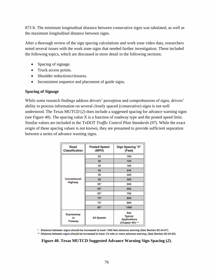
76

873 ft. The minimum longitudinal distance between consecutive signs was tabulated, as well as

the maximum longitudinal distance between signs.

After a thorough review of the sign spacing calculations and work zone video data, researchers

noted several issues with the work zone signs that needed further investigation. These included

the following topics, which are discussed in more detail in the following sections:

• Spacing of signage.

• Truck access points.

• Shoulder reductions/closures.

• Inconsistent sequence and placement of guide signs.

Spacing of Signage

While some research findings address drivers’ perception and comprehension of signs, drivers’

ability to process information on several closely spaced (consecutive) signs is not well

understood. The Texas MUTCD (2) does include a suggested spacing for advance warning signs

(see Figure 40). The spacing value X is a function of roadway type and the posted speed limit.

Similar values are included in the TxDOT Traffic Control Plan Standards (97). While the exact

origin of these spacing values is not known, they are presumed to provide sufficient separation

between a series of advance warning signs.

Figure 40. Texas MUTCD Suggested Advance Warning Sign Spacing (2).

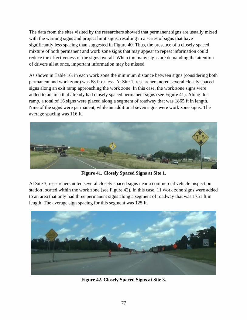
77

The data from the sites visited by the researchers showed that permanent signs are usually mixed

with the warning signs and project limit signs, resulting in a series of signs that have

significantly less spacing than suggested in Figure 40. Thus, the presence of a closely spaced

mixture of both permanent and work zone signs that may appear to repeat information could

reduce the effectiveness of the signs overall. When too many signs are demanding the attention

of drivers all at once, important information may be missed.

As shown in Table 16, in each work zone the minimum distance between signs (considering both

permanent and work zone) was 68 ft or less. At Site 1, researchers noted several closely spaced

signs along an exit ramp approaching the work zone. In this case, the work zone signs were

added to an area that already had closely spaced permanent signs (see Figure 41). Along this

ramp, a total of 16 signs were placed along a segment of roadway that was 1865 ft in length.

Nine of the signs were permanent, while an additional seven signs were work zone signs. The

average spacing was 116 ft.

Figure 41. Closely Spaced Signs at Site 1.

At Site 3, researchers noted several closely spaced signs near a commercial vehicle inspection

station located within the work zone (see Figure 42). In this case, 11 work zone signs were added

to an area that only had three permanent signs along a segment of roadway that was 1751 ft in

length. The average sign spacing for this segment was 125 ft.

Figure 42. Closely Spaced Signs at Site 3.

78

The most sign-cluttered areas in the work zones tended to be in the project limit signage area.

Figure 39 shows a sample layout. The first two signs in the series are the OBEY WARNING

SIGNS/STATE LAW (R20-3T) sign (shown in Figure 43a) and the STAY ALERT/TALK OR

TEXT LATER (G20-10T) sign (shown in Figure 43b). The effectiveness of these signs is not

known, but their necessity and value should be considered. The Texas Driver Handbook requires

drivers to obey all warning and regulatory signs (98), while current state law prohibits the use of

wireless communications devices for texting while driving (99). The use of multiple general

warning signs at the beginning of each work zone might mask other warning and regulatory

signs in the same area that direct the driver to take specific actions, such as reducing speed or

changing lanes.

(a) R20-3T Sign. (b) G20-10T Sign.

Figure 43. R20-3T and G20-10T Signs (2, 100).

The BEGIN WORK ZONE (G20-9TP) and BEGIN ROAD WORK (G20-5T) signs mark two

different locations; the former notes the point at which traffic fines may double if workers are

present, while the latter indicates the actual CSJ limit. While each sign serves separate functions,

it is not known if drivers understand the difference or think that the same information is being

repeated on another sign. A similar situation exists at the end of the project where the END

ROAD WORK (G20-2) and END WORK ZONE (G20-2bT) signs appear at the CSJ limit and at

the end of double traffic fines, respectively.

Researchers noted that in some cases, it did appear that contractors coordinated signage to

minimize clutter and confusion when transitioning between adjacent work zones. This effectively

eliminated five or more work zone signs in each direction when the same contractor was working

on two adjacent projects.

Truck Access Points

Researchers found some variations in the signage used to indicate work vehicle access points.

Signage at Sites 3 and 4 included the use of warning signs to inform drivers that there may be

79

work vehicles entering and exiting the travel lanes. Figure 44 shows a sign used at Site 3

(TRUCKS ENTERING/EXITING HIGHWAY), and Figure 45 shows a sign used at Site 4

(TRUCKS ENTERING/EXITING ROADWAY). The sign legend and layout were different for

each sign.

Figure 44. Trucks Entering/Exiting Highway Sign at Site 3.

Figure 45. Trucks Entering/Exiting Roadway Sign at Site 4.

Figure 46 shows a detailed drawing of the CW27-1T sign from TxDOT’s Standard Highway

Sign Designs for Texas manual (100). The sign legend height is 6 inches, and the overall sign

dimensions are 48 inches by 48 inches, which are the same dimensions that the Texas MUTCD

specifies for freeways and expressways. While the legend height and dimensions of the signs in

Figure 44 and Figure 45 are not known, the legend does contain more information than the sign

shown in Figure 46. Adding words to the sign legend may have reduced the legend height,

making it more difficult for drivers to read these signs, especially at higher speeds. While the

dual message sign may provide more flexibility for the contractor, it also provides less specific

information for drivers.

80

Figure 46. Trucks Entering Roadway Sign (CW27-1T) (100).

While measurements of the specific geometries at each truck access point were not possible with

the data collection methods used by the team, researchers observed that some access points had

little or no acceleration lane for work vehicles entering the open traffic lanes. At Site 3,

researchers found that there was an opening in the concrete barrier (see Figure 47) located just

downstream of the sign shown in Figure 44. The geometric design of the opening indicated that

it was for trucks entering the open traffic lane, but the access point was blocked with

channelizing drums and did not appear to be in use on the day this work zone was visited. The

credibility of the truck access point warning sign may be diminished if the sign remains in place

while the access point is not in use. The TxDOT BC Temporary Sign Notes Standard Sheet BC

(4)-14 (0) (101) states that when sign messages may be confusing or do not apply, the signs shall

be removed or completely covered.

Figure 47. Truck Entrance at Site 3.

81

Shoulder Reductions/Closures

Researchers found signage inconsistencies in areas where shoulder widths were reduced and/or

the shoulder was closed. Typically, the minimum shoulder width on freeways and expressways is

10 ft. When a work zone is present, the contractor often uses a concrete traffic barrier to provide

separation between the live traffic lanes and the work space. Placement of this barrier often

reduces the shoulder width significantly. As shown in Figure 48, the Texas MUTCD includes

two warning signs for shoulder closures.

(a) CW21-5a Sign. (b) CW21-5b Sign.

Figure 48. Texas MUTCD Warning Signs for Shoulder Closures (2).

Researchers found several examples where alternative signs were used to indicate that the

shoulder was narrow, unpaved, reduced, or closed (see Figure 49, Figure 50, and Figure 51 for

examples). At Site 3, a NARROW SHOULDER AHEAD sign was located approximately 400 ft

upstream of an unpaved shoulder (see Figure 49). Approximately 800 ft downstream of this sign

and 400 ft after the unpaved shoulder began was an UNPAVED SHOULDER sign (see

Figure 50). The placement of these signs may not have provided an accurate advance warning for

the condition.

At Site 4, a RIGHT SHOULDER REDUCED sign was used to warn drivers that the shoulder

width was changing (see Figure 51). The shoulder was less than 10 ft wide at the sign and was

approximately 2 ft wide about 100 ft downstream of the sign. A RIGHT SHOULDER CLOSED

warning sign was used for a similar condition located elsewhere in the work zone at Site 4.

82

Figure 49. Narrow Shoulder Ahead Warning Sign at Site 3.

Figure 50. Unpaved Shoulder Warning Sign at Site 3.

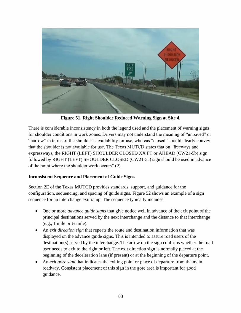
83

Figure 51. Right Shoulder Reduced Warning Sign at Site 4.

There is considerable inconsistency in both the legend used and the placement of warning signs

for shoulder conditions in work zones. Drivers may not understand the meaning of “unpaved” or

“narrow” in terms of the shoulder’s availability for use, whereas “closed” should clearly convey

that the shoulder is not available for use. The Texas MUTCD states that on “freeways and

expressways, the RIGHT (LEFT) SHOULDER CLOSED XX FT or AHEAD (CW21-5b) sign

followed by RIGHT (LEFT) SHOULDER CLOSED (CW21-5a) sign should be used in advance

of the point where the shoulder work occurs” (2).

Inconsistent Sequence and Placement of Guide Signs

Section 2E of the Texas MUTCD provides standards, support, and guidance for the

configuration, sequencing, and spacing of guide signs. Figure 52 shows an example of a sign

sequence for an interchange exit ramp. The sequence typically includes:

• One or more advance guide signs that give notice well in advance of the exit point of the

principal destinations served by the next interchange and the distance to that interchange

(e.g., 1 mile or ½ mile).

• An exit direction sign that repeats the route and destination information that was

displayed on the advance guide signs. This is intended to assure road users of the

destination(s) served by the interchange. The arrow on the sign confirms whether the road

user needs to exit to the right or left. The exit direction sign is normally placed at the

beginning of the deceleration lane (if present) or at the beginning of the departure point.

• An exit gore sign that indicates the exiting point or place of departure from the main

roadway. Consistent placement of this sign in the gore area is important for good

guidance.

84

Figure 52. Interchange Exit Ramp Sign Sequence from Texas MUTCD (2).

A similar sequence of signs (i.e., advance guide sign, exit direction sign, and exit gore sign)

should be present at exits in work zones. Researchers found instances where the signage did not

include the standard sequence of exit signs. At one location at Site 3, the exit ramp locations for

three crossing roadways had been moved to a single exit. The images in Figure 53a and

Figure 53b show the advance guide signs, while Figure 53c shows the exit direction sign located

where the exit gore sign typically would have been placed. A review of the constructions plan

sheets for this project showed that the signs were placed in accordance with those plans (see

Figure 54). Even so, the location of this exit direction sign violates driver expectancy, given that

drivers normally see this sign before the need to make an exit maneuver. In addition, the Texas

MUTCD states that “no more than two destination names or street names should be shown on

any advance guide sign or exit direction sign” (2). Thus, the sign design also violates the

suggested limit on the amount of information that should be presented to drivers with freeway

signs.

In another example, researchers found that the advance guide sign was missing from an exit sign

sequence. Figure 55 shows the exit direction and exit gore signs for the Chew Road exit, but no

advance guide sign was present to provide information about the upcoming exit.

In yet another example, researchers found that the exit gore sign was missing from an exit sign

sequence. Figure 56 shows the exit gore sign missing from one of the exits at Site 4.

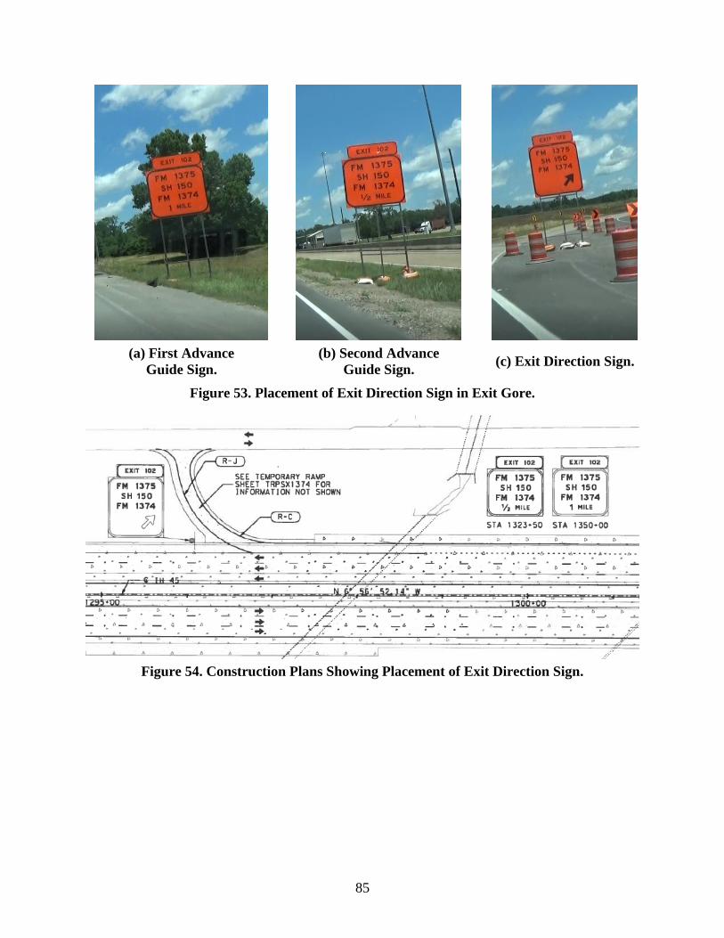
85

(a) First Advance

Guide Sign.

(b) Second Advance

Guide Sign. (c) Exit Direction Sign.

Figure 53. Placement of Exit Direction Sign in Exit Gore.

Figure 54. Construction Plans Showing Placement of Exit Direction Sign.

86

Figure 55. Exit Direction and Exit Gore Signs at Site 4.

Figure 56. Exit Gore Sign Missing at Site 4.

RECOMMENDATIONS

After a review of the issues, researchers developed several recommendations that are organized

by topic below.

Spacing of Signage

Recommendations concerning sign spacing include the following:

• Consider reviewing the project limit signs (from a driver’s perspective) to determine if all

are warranted.

87

• As part of the design process, consider the presence of permanent signs that will remain

in place during construction when deciding where to locate work zone signs.

Truck Access Points

Recommendations concerning truck access points include the following:

• Ensure that all truck access point warning signs meet minimum size requirements.

• Consider the use of separate warning signs for trucks entering and trucks exiting to

maintain sign legibility and provide more accurate information to drivers.

• Remove or completely cover truck access warning signs when the access point is not in

use.

• Consider use of a sign comprehension study to better understand how drivers respond to

various types of truck warning messages.

• Consider the use of dynamic truck warning systems to provide more real-time warnings

to drivers. TxDOT’s Smart Work Zone Guidelines (102) provides an implementation

decision-making framework that may be useful.

• Consider improving geometric design of truck acceleration and deceleration lanes.

Guidance can be found in the Designing Work Space Access Points to Better

Accommodate Large Trucks (103) publication from the American Road and

Transportation Builders Association.

Shoulder Reductions/Closures

Recommendations concerning shoulders include the following:

• Use of signs indicating a narrow shoulder may not provide enough information for

drivers to decide if the shoulder is available for their use. Instead, consider RIGHT

(LEFT) SHOULDER CLOSED or NO SHOULDER signs.

• Be consistent in placement of the RIGHT (LEFT) SHOULDER CLOSED AHEAD and

RIGHT (LEFT) SHOULDER CLOSED signs. This may provide more accurate

information and sufficient advance warning for drivers.

• Consider use of a sign comprehension study to better understand how drivers respond to

various types of shoulder reduction and closure warning messages.

Inconsistent Sequence and Placement of Guide Signs

Recommendations concerning the sequence and placement of guide signs include the following:

• Designers should follow the guidance set forth in the Texas MUTCD.

• Inspectors should ensure that signs are placed in accordance with the project plans.

89

CHAPTER 8:

EFFECTIVENESS OF PEDESTRIAN CROSSING TREATMENTS

AT NIGHT

One reason that motor vehicle crashes with pedestrians are a concern is that pedestrians are more

likely to sustain fatal or severe injuries compared to vehicle occupants. In Texas between 2010

and 2016, pedestrian crashes accounted for 3434 fatal crashes, representing 16 percent of all fatal

crashes (104). A large majority of those pedestrian fatal crashes occurred during the nighttime

(79 percent).

Several traffic control device treatments aimed at improving crossing opportunities for

pedestrians have been installed including the following:

• Pedestrian hybrid beacon (PHB) (see the example in Figure 57a).

• Rectangular rapid flashing beacon (RRFB) (see the example in Figure 57b).

• Light-emitting diode embedded (LED-Em) pedestrian/school crossing sign (see the

example in Figure 57c).

Figure 57. Examples of Treatments.

(a) PHB. (b) RRFB.

(c) LED-Em.

90

While the effectiveness of the PHB, RRFB, and LED-Em have been examined in previous

studies, whether these treatments have a similar effectiveness at night had yet to be explored. For

this activity, researchers sought to evaluate and compare the day and night operational

performance of the PHB, RRFB, and LED-Em treatments.

PREVIOUS RESEARCH

Several studies have examined the operational performance of pedestrian traffic control device

crossing treatments including a 2019 TxDOT study that summarized the findings for these three

treatments (105, 106). Most of these studies used a study approach of counting the number of

drivers that did and did not yield to a crossing pedestrian. In many cases a staged pedestrian, who

is a researcher trained to cross in a similar manner for all locations and crossings, was used. A

summary of key findings for each of the treatments follows.

PHBs

Several studies have evaluated PHBs and have reported high yielding rates varying from 75 to

97 percent (107, 108, 109). A comprehensive study for FHWA (110) identified an overall

average driver yield rate of 96 percent for sites with posted speed limits between 30 and 45 mph.

An Arizona Department of Transportation study (111) used 10 locations in Arizona for which

operating speeds ranged between 44 mph and 54 mph to evaluate the driver yielding rates for

facilities with higher posted speed limits. The researchers found that the average yield rate across

the sites was 97 percent, thus concluding that PHBs are equally effective on facilities with higher

posted speed limits.

RRFBs

A 2016 TTI report (112) that evaluated the effectiveness of RRFBs provides a detailed summary

of various studies that investigated the effectiveness of RRFBs using the measure of driver yield

rates. These studies were also summarized in a previous-year TxDOT report (105). Before-after

studies reported increased yielding rates although with large variability in the magnitude of the

increase. Other studies, which examined the yield rate at treated sites with either staged or non-

staged pedestrian observations, also found a wide range of effectiveness, varying by time of day,

treatment activation, beacon location, and shape. The TTI study (112) combined previous data

from TxDOT and FHWA studies and, through a series of statistical models, identified factors

associated with driver yielding at the RRFB. Those factors included intersection configuration

(number of legs), presence of median, crossing distance, and direction of travel (one-way versus

two-way traffic). For a subset of data that included 1-minute vehicle counts for each crossing, the

statistical model showed several significant factors contributing to driver yielding such as

intersection configuration, crossing distance, 1-minute traffic count, posted speed limit, location

of the beacons (overhead or roadside), sign face, and presence of yield line, school, or transit

stop.

91

LED-Ems

Most previous studies on the LED-Em pedestrian/school crossing signs only included a few

locations (113, 114, 115). These studies found, in general, low driver yielding. At a crosswalk

with an LED-Em in Des Moines (113), motorist yielding observed was highest in the morning at

46 percent, followed by lower yielding rates of 40 percent at noon and 30 percent in the

afternoon. The Vermont case study (114) noted that overall yield rate decreased at the site from

year one to year four of installation, but still remined 12 percent higher than the yield rate before

installation. Observations at the Maple Grove, Minnesota, site (115) included no improvement in

driver yield rates after the installation of the LED-Em and less than 20 percent of pedestrians

activating the treatment during crossings.

The Texas study (105, 106) collected data at several LED-Em installations. Higher hourly

volumes, speeds 45 mph and greater, lack of sidewalks, and 12-ft lanes (no deviation from

baseline 12-ft lane width) were found to adversely affect yield probability. The authors

concluded that based on the findings, LED-Em would be a suitable candidate treatment at sites

with sidewalks, lower operating speeds and traffic volumes, and narrow lanes.

Key Findings from Literature

The main findings from the literature review included the following:

• None of the previous research efforts included nighttime data collection.

• PHBs have been found to have very high driver yielding rates including sites with wider

crossing distances and operating speeds up to 54 mph, making PHBs a preferred

treatment for higher-speed/multilane roadways.

• While RRFBs have been shown to be an effective treatment, several studies have

demonstrated a wide range of effectiveness. The treatment was found to be more

effective for crossings with shorter crossing distance and presence of a median, with the

presence of a yield line, and near a school or transit stop.

• Most of the studies on the effectiveness of LED-Ems only included a few locations. The

2019 TxDOT study (105) collected data at 13 locations and found an average driver yield

rate of 40 percent.

These findings suggested that in the examination of nighttime conditions, study site selection

should consider a range of geometric conditions including number of lanes (crossing distance),

median presence, and speed (operating or posted).

STUDY APPROACH

Researchers employed a staged pedestrian crossing study approach in this study. The intent was

to collect data at 30 sites during both daytime and nighttime conditions; however, equipment

malfunctions and, in a few cases, concerns with the available nighttime street lighting conditions

92

limited nighttime data collection at some sites. The following sections describe site selection, site

characteristics, data collection methodology, and data reduction processes.

Site Selection

Several locations with the pedestrian treatment of interest were known due to recent TTI research

in this topic area. The researchers also identified locations, especially for the RRFB, through a

Texas District of the Institute of Transportation Engineers e-newsletter request.

The goal was to select 10 sites for each of the treatments of interest. Sites were selected with

consideration of having a range of posted speed limits and median types represented. In addition,

sites were selected to represent either two- or four-lane roads. Data collection efficiency was the

final consideration in site selection. For the LED-Em treatment, all feasible sites were

considered. The sites with PHBs were concentrated in Austin, which reflects the city with the

most PHB installations in Texas. More regions within Texas have installed the RRFB (and the

LED-Em), and the site selection reflected that diversity.

Site Characteristics

Researchers collected data at 10 PHB sites, 12 RRFB sites, and eight LED-Em sites. The

daytime data collected at 12 LED-Em sites in the late spring of 2019 were also used in the

analysis. Researchers used aerial photographs to identify the roadway geometric characteristics,

and these characteristics were confirmed in the field as needed. Table 17 lists the variable

descriptions considered in the statistical analysis. Additional variables were collected for each

site, such as crosswalk pavement marking pattern type and distance to street light; however,

those variables were either fairly uniform for all sites or were determined in the preliminary

analyses to be not influential with respect to driver yielding.

Table 18 lists the site characteristics for the 10 PHB sites. All PHB sites had an advance stop line

and continental crosswalk pavement markings. Most had an advance warning sign. For

motorists, the PHB rests in the dark mode and when activated transitions to flashing yellow,

steady yellow, steady red, and then flashing red. The flashing yellow provides an additional

warning to the drivers that the device will soon be transiting to red. For these 10 sites the

flashing yellow lasted between 4 and 9 seconds. The flashing red ranged between 24 and

35 seconds.

Table 19 lists the site characteristics for the 12 RRFB sites. One of the sites had diagonal

crosswalk pavement markings, with all remaining sites having continental pavement markings at

the crosswalk. The length of time the device was active (i.e., flashing yellow) ranged between 25

and 35 seconds. Researchers did not collect nighttime data at one location because the equipment

had malfunctioned, and the device would not activate when the pedestrian pushed the button.

93

Table 17. Variable Descriptions.

Variable,

Variable Name Description

Active Speed Limit

Group,

ActiveSpeedLimitGroup

Speed limits grouped into low (35 mph and less) or high (40 mph and

more).

Active Speed Limit,

ActiveSpeedLimit Speed limit active during data collection (mph). One of the LED-Em sites

was within an active school zone, and the school zone speed limit of 20 mph

was used in the statistical analysis rather than the posted speed limit of 30

mph. Variable used as a surrogate for typical operating speeds.

Advance Sign,

AdvanceSign

Is an advance warning sign present for the site (yes=advance sign or no)?

Bike Lane, BikeLane Bike lane presence (none, 1 side, or 2 sides).

Hourly Volume,

HourlyVol

Estimated hourly volume just prior to the staged pedestrian crossing,

determined by expanding the number of vehicles driving over the crosswalk

(both directions) during the 1 minute prior to the staged pedestrian crossing

(veh/hr).

Lane Width Group,

LnWdGroup

Lane width grouped into narrow (10.5 or 11 ft), typical (11.5 or 12 ft), or

wide (13 ft or more).

Lane Width, LnWd Lane width (ft).

Legs Number of legs where two legs are a midblock crossing, three legs are a

T intersection, and four legs are a cross intersection.

Light level, LightLevel Natural light level during data collection (day or night).

Median Type, MedType Type of median (raised, two-way left-turn lane [TWLTL], or none).

Develop Type of development such as whether the intersection is near a major

development, such as commercial, hospital/university (Hos/Univer),

residential, or mix.

Number of Through

Lanes, #ThruLanes

Number of through lanes on the major road, total of both directions, ranges

from two to four lanes, with one site having five lanes.

Parking Lane, ParkLane Parking lane presence (none, one side, or two sides).

Posted Speed Limit,

PSL

Posted speed limit (mph).

Site Code Two-letter city code, and two- or three-digit site number.

Treatment Type,

TreatType

Type of treatment (PHB, RRFB, or LED).

Yield or Stop Line, Line Presence of a stop or yield line prior to the crosswalk (stop [only PHBs],

yield [for RRFBs or LED-Ems], or none). Stop lines may be used to indicate

the point behind which vehicles are required to stop in compliance with a

traffic control device that requires vehicles to stop. Yield lines may be used

to indicate the point behind which vehicles are required to yield.

94

Table 18. Site Characteristics for the PHB Sites.

Site Code1 #Thru

Lanes

LnWd

(ft) PSL Legs MedType AdvanceSign Line Develop

AU-001 5 10 40 3 Raised Yes Stop Commercial

AU-013 4 11 40 2 TWLTL Yes Stop Commercial

AU-014 2 10 35 2 None Yes Stop Commercial


AU-035 4 9.5 35 2 None Yes Stop Commercial


AU-045 4 11 40 4 None Yes Stop Commercial

AU-066 4 11 45 4 Raised Yes Stop Residential

AU-067 2 11 30 2 TWLTL Yes Stop Residential

AU-068 4 9 40 3 TWLTL Yes Stop Commercial 1 Variable description available in Table 17.

Table 19. Site Characteristics for the RRFB Sites.

Site Code1 #Thru

Lanes

LnWd

(ft) PSL Legs MedType AdvanceSign Line Develop

AU-004 2 10 30 4 Raised No Yield Residential

DEN-01 4 9.5 30 3 Raised Yes Yield Commercial

GA-002 4 11 40 4 Raised Yes Yield Residential

GA-006 4 11 40 4 Raised No Yield Residential


GA-010 4 11.5 40 4 Raised Yes Yield Residential


MA-002 2 14 30 3 None Yes None Hos/Univer

SA-002 4 12 40 3 Raised Yes Yield Residential

SA-005 2 13.5 30 4 Raised Yes None Hos/Univer

SA-006 2 14 30 3 Raised Yes None Hos/Univer

CS-003 2 12 30 3 TWLTL No None Hos/Univer 1 Variable description available in Table 17.

Table 20 provides the site characteristics for the LED-Em sites. Because of challenges during

data collection, attempts to collect data between November 2019 and February 2020 occurred at

eight rather than the preferred 10 sites. The daytime data collected at 12 sites during the May

2019 study (105) were included in the analysis to expand the sample size. Additional challenges

were faced with regards to the nighttime data collection for the LED-Em sites. At two of the

sites, the data collectors did not feel comfortable with the combination of operating speed,

available street light levels for both sides of the street, type of development, and/or lack of

general pedestrian activity level; therefore, nighttime data collection was stopped at those two

sites. Table 20 indicates if the data available for analysis represented:

• Daytime data collected in the spring of 2019.

• Daytime data collected in the winter of 2019–2020.

• Nighttime data collected in the winter of 2019–2020.

95

At one of the sites, the LEDs flashed for 80 seconds upon activation. The other sites where the

flash rate was known had a range of 30 to 60 seconds for the length of time the LEDs were

flashing.

Table 20. Site Characteristics for the LED-Em Sites.

Site Code1 Data

Source2

#Thru

Lanes

LnWd

(ft) PSL Legs MedType

Advance

Sign Line Develop

CB-001 A, B, C 4 12 35 3 TWLTL Yes None Residential

CB-002 A, B 4 12 35 4 TWLTL Yes None Residential

CS-001 A, C 4 11 30 2 Raised Yes Yield University

DF-001 A, B, C 4 12 45 2 TWLTL Yes None Mix

HS-001 A 2 12 50 4 None No None Residential

KT-001 A 4 12 35 3 Raised No Yield Residential

NB-001 A, B, C 2 11.5 30 3 None Yes None Residential

NS-001 A, B, C 4 10.5 30 3 None No None Commercial

RW-001 A 2 11 50 3 TWLTL No None Residential

SA-001 A, B 4 12 35 2 Raised Yes Yield Commercial

SA-002 A 2 12 30 2 None No None Commercial

SP-001 A, B, C 4 12 30 3 Raised Yes None Residential

YT-001 A 2 11 303 4 None No None Mix 1 Variable description available in Table 17. 2 Time period for data collection, where A = daytime, spring 2019; B = daytime, winter 2019–2020; and

C = nighttime, winter 2019–2020. 3 Site was in a school zone that was active during data collection; therefore, an active speed limit of 20 mph was

used in the statistical analysis.

Data Collection Protocol

The protocol for data collection was developed and refined based on experiences from several

previous research projects (106, 110, 116). For this study, a goal of 60 staged pedestrian crossing

events or 4 hours of data (the smaller of the two) were collected at each location. A staged

pedestrian is a member of the research team who wears a “uniform” of gray t-shirt or sweatshirt,

blue jeans, and predominantly dark shoes while completing the street crossings. A baseball cap

and sunglasses are permitted. The staged pedestrian is trained to approach the crossing in a

similar manner for each location to minimize the effects of pedestrian behavior on drivers.

Training also covers when the staged pedestrian should approach the pedestrian push button so

there is at least one driver who must decide whether to yield or not yield to the waiting

pedestrian once the treatment is activated. Placing a foot on the pavement is also part of the

training so that the staged pedestrian meets the state law requirement that the pedestrian needs to

be on the pavement (rather than just waiting on the curb).

The staged pedestrian activates the pedestrian treatment and then waits until the vehicular traffic

approaching has stopped before initiating the crossing. For the next staged pedestrian crossing

event, the staged pedestrian is to have at least 1 minute between events so that all queued

vehicles clear before beginning another staged crossing. The 1-minute gap also permits the

96

counting of the number of vehicles present at the site without including vehicles being in a queue

for a previous crossing pedestrian.

The second member of the research team waits in an area where he or she will not attract the

attention of drivers or natural pedestrians while at the same time having a clear view of the

crosswalk, pedestrians, and traffic from both directions. This person records the number of

drivers that did not and did yield to the staged pedestrian.

A video camera was also installed prior to data collection. The recordings served as a backup for

the yielding data collected and were used to obtain the 1-minute volume vehicle counts prior to

each pedestrian crossing. While the site could be within a school zone, researchers attempted to

collect data when the school zone was not active. Researchers collected data when a school zone

was active at only one site (YT-01), and the school zone speed limit was used in the analysis

rather than the posted speed limit.

Data Collection

For this research effort, researchers began collecting data in November 2019 and completed the

data collection in February 2020. Data from a previous effort (collected May 2019) were also

included in the statistical analysis. The video camera was arranged to capture the crosswalk

markings and the pedestrian crossings along with the treatment, as possible (see the example in

Figure 58).

Figure 58. Example of Video Camera View.

This study included about 224 hours of video recordings. The previous TxDOT study provided

about 48 hours of video (105). Table 21 summarizes the number of staged pedestrian crossings

along with the total number of drivers reacting to the staged pedestrians by treatment type, light

97

level, and data collection period. Data for 9301 drivers over 3871 pedestrian crossings were

reduced.

Table 21. Number of Staged Pedestrian Crossings and Drivers Included in Analysis.

Current or

Previous

Study

Data Collection

Dates

Treatment

Type

Daytime

Number of

Staged

Pedestrian

Crossings

Nighttime

Number of

Staged

Pedestrian

Crossings

Daytime

Number

of Drivers

Nighttime

Number

of Drivers

Current November

2019–February

2020

PHB 570 623 1,746 1,623

RRFB 709 546 1,420 980

LED-Em 421 326 1,523 579

Subtotal 1,700 1,495 4,689 3,182

Previous May 2019 LED-Em 676 0 1,430 0

Total used

in analysis

Grand total All 2,376 1,495 6,119 3,182

Video Data Reduction

Video data reduction primarily focused on obtaining 1-minute volume counts. The video was

also used to confirm the driver yielding or not yielding data for several sites because the video

permitted replaying of the recording, which allowed for better quality control, especially at the

PHB sites.

Researchers used the video to count the number of vehicles driving across the crosswalk for

1 minute prior to each staged pedestrian crossing. The 1-minute increment provides an

appreciation of the amount of traffic present during the crossing. The theory is that with more

vehicles, drivers may be hesitant to stop for the pedestrian because of a concern with being rear-

ended. Video player software with the capability to advance the video footage on a frame-by-

frame basis was used. In general, the researcher identified the video frame during which the

staged pedestrian pressed the button to activate the treatment and then rewound the video for at

least 1 minute. In a few cases, a slightly longer time period was used to be able to avoid starting

the count with a vehicle on the crosswalk. There were also a few cases when a shorter time

period was used because of the timing of the previous staged pedestrian crossing and the

presence of a queue discharge or because of the start time of the video file.

Researchers converted the 1-minute traffic counts into hourly volumes by using the exact

number of seconds reflected in the vehicle count. Table 22 provides the minimum, maximum,

and average hourly vehicle counts by site and light level.

98

Table 22. Hourly Vehicle Volume (Minimum, Maximum, and Average) Calculated Based

on 1-Minute Count Prior to Pedestrian Staged Crossing.

Treatment

Type Site

Daytime

Min.

Daytime

Max.

Daytime

Average

Nighttime

Min.

Nighttime

Max.

Nighttime

Average

PHB AU-001 514 3,240 1,739 240 2,700 1,001

AU-013 48 960 488 60 660 261

AU-014 120 1,800 613 60 900 239

AU-027 240 2,040 1,231 240 1,680 896

AU-035 456 3,180 1,759 304 3,660 1,802

AU-042 60 900 484 120 1,020 570

AU-045 120 1,140 453 60 1,440 439

AU-066 171 1,620 809 180 2,040 870

AU-067 60 840 458 60 420 149

AU-068 1,320 6,930 3,741 960 5,100 3,287

PHB Total 48 6,930 1,545 60 5,100 1,305

RRFB AU-004 60 720 351 51 540 257

CS-03 120 1,020 525 60 540 188

DEN-01 120 2,700 799 101 2,700 444

GA-002 240 1,560 901 120 1,440 666

GA-006 60 780 324 60 840 333

GA-007 120 2,160 936 240 1,980 978

GA-010 60 540 268 60 900 281

GA-013 300 1,800 843 240 1,140 690

MA-002 180 900 453 60 420 124

SA-002 120 1,440 703 120 2,280 930

SA-005 420 1,380 835 ND ND ND

SA-006 51 300 118 60 240 120

RRFB Total 51 2,700 658 51 2,700 518

LED-Em CB-01 120 840 404 40 360 161

CB-02 152 1,260 609 ND ND ND

CS-01 43 1,984 437 60 480 178

DF-01 180 1,071 594 60 900 437

HS-01 31 1,516 686 ND ND ND

KT-01 137 835 438 ND ND ND

NB-01 26 544 177 60 240 88

NS-01 240 1,800 849 60 900 413

RW-01 86 800 482 ND ND ND

SA-01 558 2,700 1,633 ND ND ND

SA-02 17 880 354 ND ND ND

SP-01 60 1,035 351 60 900 280

YT-01 153 1,020 539 ND ND ND

LED-EM Total 17 2,700 776 40 900 299

ND = no data collected at this site/light level

99

ANALYSIS

Because staged pedestrian crossings are more uniform than the non-staged crossings and only a

few non-staged pedestrian crossings were observed during data collection (i.e., a small sample

size), the researchers only used data for staged crossings in the analysis. Data were collected by

pedestrian crossing event where the number of vehicles yielding and not yielding was recorded.

This format was revised to reflect the decision of each driver so that each driver was assigned a

value of 1 if yielding or a value of 0 if not yielding.

The objective of this analysis was to explore the relationship between driver yielding and

independent variables and assess their effects on the probability of driver yielding. Because the

outcome variable is dichotomous (i.e., did the driver yield or not yield), a logistic regression

model was employed.

The log-odds of the probability of driver yielding given the value of independent variables (X),

( )P Y Yield x= , can be expressed as follows:

( )( )( ) 0 1 1ln

1k k

P Y Yieldg x x

P Y Yield

== = + +

− =

xx

x ,

where g(x) is the logit (log-odds), x denotes a value of the independent variables 1, , kX X

(such as TreatType, LightLevel, ActiveSpeedLimit, HourlyVol, Legs, #ThruLanes, Line, etc.).

The logit, g(x), is linear in its parameters. The intercept 0 represents the baseline level of the

logit, and k represents the change in the logit that occurs with a unit change in kX . The

conditional probability that the driver yields at site i in the jth pedestrian crossing can be

expressed as

𝑃(𝑌𝑖𝑗 = 𝑌𝑖𝑒𝑙𝑑|𝑥) =𝑒𝑔(𝑥)

1+𝑒𝑔(𝑥) =𝑒

𝛽0+𝛽1𝑥𝑖,1𝑗⋯+𝛽𝑘𝑥𝑖,𝑘𝑗

1+𝑒𝛽0+𝛽1𝑥𝑖,1𝑗⋯+𝛽𝑘𝑥𝑖,𝑘𝑗

.

To account for possible correlation in the outcome variable obtained for multiple time periods

(multiple crossings) from the same site, the generalized estimating equations (GEE) are

employed as an estimation method.

Prior to conducting the logistic regression, preliminary analyses were performed using a normal

linear model, specifically the analysis of covariance model, applied to driver yielding rates

averaged by each site and light level. A normal linear (i.e., analysis of covariance [ANCOVA])

model was considered since many of the independent variables are site based rather than

individual crossing event based, and the average driver yielding rates satisfy the underlying

assumptions for the normal linear models. The results from a linear model are also easier to

interpret when considering whether the findings are reasonable.

100

The following section summarizes the findings from the two statistical analysis techniques

selected for this study:

• An ANCOVA model based on mean yield rates where the average is taken over all

staged crossings at each site by light level.

• A logistics regression model based on individual driver response to a staged pedestrian

crossing.

RESULTS

Average Driver Yielding Rate per Site

Each driver responding to a staged pedestrian crossing was coded as being either 1 (for yielding)

or 0 (for not yielding). The average driver yielding rate (DYR) was calculated by:

𝐷𝑌𝑅 =∑ 𝑁𝑢𝑚𝑏𝑒𝑟 𝑜𝑓 𝐷𝑟𝑖𝑣𝑒𝑟𝑠 𝑌𝑖𝑒𝑙𝑑𝑖𝑛𝑔

∑ 𝑇𝑜𝑡𝑎𝑙 𝑁𝑢𝑚𝑏𝑒𝑟 𝑜𝑓 𝐷𝑟𝑖𝑣𝑒𝑟𝑠

Table 23 lists the average DYR by site and by treatment type for daytime and nighttime

conditions, and Figure 59 illustrates the same data. Table 23 also provides the DYR difference

between nighttime and daytime for each site. The distribution of daytime average DYRs for this

study is similar to previous studies with the following observations:

• PHB—the average DYR is high (a range of 95 to 100 percent with the average being

97 percent).

• RRFB—a large range (60 to 90 percent) with an average (77 percent) below the yielding

rate for the PHBs.

• LED-Em—an even larger range (5 to 84 percent) compared to RRFBs and PHBs with an

overall daytime average (29 percent) below both the PHBs and RRFBs.

The focus of this research effort was on nighttime conditions as compared to daytime conditions.

Table 23 shows that the overall average DYRs for nighttime conditions are generally like the

rates observed for daytime conditions. For PHBs, the rates appear to be very similar (i.e., an

average of 97 percent for daytime and 96 percent for nighttime across all PHB sites, and within

each site the daytime and nighttime rates are similar).

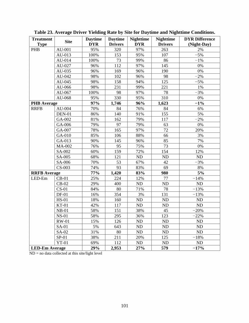
101

Table 23. Average Driver Yielding Rate by Site for Daytime and Nighttime Conditions.

Treatment

Type Site

Daytime

DYR

Daytime

Drivers

Nighttime

DYR

Nighttime

Drivers

DYR Difference

(Night-Day)

PHB AU-001 95% 320 97% 263 2%

AU-013 100% 153 95% 107 −5%

AU-014 100% 73 99% 86 −1%

AU-027 96% 112 97% 145 0%

AU-035 96% 169 96% 190 0%

AU-042 98% 102 96% 98 −2%

AU-045 98% 158 94% 125 −5%

AU-066 98% 231 99% 221 1%

AU-067 100% 98 97% 78 −3%

AU-068 95% 330 95% 310 0%

PHB Average 97% 1,746 96% 1,623 −1%

RRFB AU-004 70% 84 76% 84 6%

DEN-01 86% 140 91% 155 5%

GA-002 81% 162 79% 117 −2%

GA-006 79% 97 79% 63 0%

GA-007 78% 165 97% 72 20%

GA-010 85% 106 88% 66 3%

GA-013 90% 145 96% 85 7%

MA-002 76% 95 75% 73 0%

SA-002 60% 159 72% 154 12%

SA-005 68% 121 ND ND ND

SA-006 70% 53 67% 42 −3%

CS-003 74% 93 83% 69 8%

RRFB Average 77% 1,420 83% 980 5%

LED-Em CB-01 25% 224 12% 77 −14%

CB-02 29% 400 ND ND ND

CS-01 84% 80 71% 78 −13%

DF-01 16% 354 3% 131 −13%

HS-01 18% 160 ND ND ND

KT-01 42% 117 ND ND ND

NB-01 58% 151 38% 45 −20%

NS-01 58% 295 36% 123 −22%

RW-01 15% 126 ND ND ND

SA-01 5% 643 ND ND ND

SA-02 31% 80 ND ND ND

SP-01 38% 211 20% 125 −18%

YT-01 69% 112 ND ND ND

LED-Em Average 29% 2,953 27% 579 −17%

ND = no data collected at this site/light level

102

Figure 59. Driver Yielding by Treatment, Light Level, and Site.

For LED-Em also, the overall average nighttime rate looks like daytime with 29 percent of the

drivers during the day and 27 percent of the drivers during the night yielding to pedestrians.

Within each LED-Em site, however, driver yielding during the day is noticeably higher than

driver yielding during the night. In a review of the difference between nighttime and daytime

yielding within each site when nighttime data were available, those LED-Em sites appear to have

large differences between daytime and nighttime. As shown in the final column of Table 23, the

differences were between 13 and 22 percent lower nighttime driver yielding for a site. The

statistical analysis (in the following section) did find a statistically significant difference in

daytime and nighttime yielding when site-to-site variability (resulting from different site

characteristics) is incorporated into the analysis.

Previous research, along with the range of yielding rates observed, especially for the RRFB and

the LED-Em, indicates that other factors than just the subject traffic control device are

contributing to the variability of the yielding results. The next two sections discuss the findings

from the statistical evaluations that examined potential variable effects on yielding including the

key question for the research—is driver yielding different during daytime and nighttime

conditions.

ANCOVA Model Based on Mean Yield Rates for Sites and Light Level

There were repeated observations for day and night from 35 sites in the dataset. Researchers

conducted several preliminary analyses to identify the best approach and variables to include in

the statistical models. Initially, researchers considered all variables, and examined the various

combinations to identify the model that seemed to be the most appropriate in terms of model

103

goodness of fit criteria and interpretation. Researchers conducted the analysis using a mixed-

effect ANCOVA model with LightLevel (i.e., day or night) and site characteristic variables

(including TreatType, ActiveSpeedLimitGroup, and LnWdGroup as discrete factors and

Mean(HourlyVol) as a covariate) as fixed effects. Researchers also included Site Code as a

random effect to account for the fact that the values of the site characteristic variables are

repeated in the data. Two-way interaction effects between TreatType and other site characteristic

variables were included in the model to see if the effect of treatment type varies with the levels

of other site characteristic variables. Table 24 shows the estimated model coefficients, and Table

25 provides the effect tests results (based on F-tests) for the variables included in the model

shown in Table 24. LnWdGroup was included as a nested effect (i.e., effect nested within

TreatType) because the levels of LnWdGroup were different for each TreatType (i.e., PHB has

only a narrow LnWdGroup, LED-EM has narrow and typical, and RRFB has all three levels

[narrow, typical, and wide]).

Table 24. ANCOVA Model Including Treatment Type, Light Level, and Other Site

Characteristic Variables Using Per-Site Mean Yield Rates.

Parameter Estimates Estimate Std Error DFDen t Ratio Prob>|t|

Intercept 0.6982278 0.028413 33.48 24.57 <0.0001

TreatType[LED-Em] −0.430449 0.029525 26.68 −14.58 <0.0001

TreatType[PHB] 0.3071775 0.02723 23.48 11.28 <0.0001

LightLevel[Day] 0.026969 0.007159 35.91 3.77 0.0006

Mean(HourlyVol) −4.417e-5 3.91e-5 47.15 −1.13 0.2644

ActiveSpeedLimitGroup[Low] 0.0454034 0.019072 22.32 2.38 0.0262

TreatType[LED-Em]*LightLevel[Day] 0.0756203 0.011038 39.02 6.85 <0.0001

TreatType[PHB]*LightLevel[Day] −0.019354 0.009628 34.21 −2.01 0.0523

TreatType[LED-Em]*

(Mean(HourlyVol)-668.511)

−0.000145 5.828e-5 42.3 −2.49 0.0168

TreatType[PHB]*(Mean(HourlyVol)-

668.511)

3.1058e-5 4.314e-5 43.8 0.72 0.4754

TreatType[LED-Em]*

ActiveSpeedLimitGroup[Low]

0.0920804 0.026653 22.66 3.45 0.0022

TreatType[PHB]*

ActiveSpeedLimitGroup[Low]

−0.04332 0.026191 21.75 −1.65 0.1125

TreatType[LED-Em]:

LnWdGroup[narrow]

0.1355606 0.029252 22.36 4.63 0.0001

TreatType[RRFB]:LnWdGroup[narrow] 0.0298317 0.039141 21.53 0.76 0.4542

TreatType[RRFB]:LnWdGroup[typical] 0.0245799 0.044553 21.08 0.55 0.5870

Summary of Fit

RSquare 0.987749

RSquare Adj 0.984512

Root Mean Square Error 0.047239

Mean of Response 0.685299

Observations (or Sum Wgts) 68

Std Error = standard error; DFDen = degrees of freedom in denominator; t Ratio = test statistic used for the t-test;

Prob>|t| = p-value for the t-test

104

Table 25. Fixed Effect Tests for Model in Table 24.

Source Nparm DF DFDen F Ratio Prob > F

TreatType 2 2 25.09 113.2088 <0.0001

LightLevel 1 1 35.91 14.1898 0.0006

Mean(HourlyVol) 1 1 47.15 1.2759 0.2644

ActiveSpeedLimitGroup 1 1 22.32 5.6676 0.0262

TreatType*LightLevel 2 2 35.06 26.1621 <0.0001

TreatType*Mean(HourlyVol) 2 2 44.07 3.0958 0.0552

TreatType*ActiveSpeedLimitGroup 2 2 22.29 5.9805 0.0083

LnWdGroup[TreatType] 3 3 21.69 7.5270 0.0012 Nparm = number of parameters; DF = degrees of freedom; DFDen = degrees of freedom in denominator;

F Ratio = test statistics used for the F-test; Prob> F = p-value for the F-test

Table 25 shows that the interaction effects TreatType*LightLevel and

TreatType*ActiveSpeedLimitGroup as well as the main effects TreatType, LightLevel,

ActiveSpeedLimitGroup, and LnWdGroup nested within TreatType are statistically significant at

α=0.05 and TreatType*Mean(HourlyVol) is statistically significant at α=0.1. When there are

significant interaction effects, the effect of each factor involved in the interaction needs to be

assessed conditionally on the levels of the other factor because the effect might be different for

each level of the other factor. Therefore, the effect of LightLevel needed to be assessed for each

level of TreatType. Likewise, the effect of ActiveSpeedLimitGroup needed to be assessed for

each level of TreatType.

The results from Table 24 and Table 25 indicate that the effectiveness of the treatment may vary

between nighttime and daytime conditions. The results also show that speed limit groups’ and

lane width groups’ influence on driver yielding may vary by treatment type. Least square means

(LSM) are predicted values of the response (DYR). When there are multiple factors in the model,

it is not fair to make comparisons between raw cell means in data because raw cell means do not

compensate for other factors in the model. The LSM are the predicted values of the response for

each level of a factor that have been adjusted for the other factors in the model.

Figure 60 shows the plots for the comparison of daytime and nighttime LSM DYRs by treatment

type. The plot shows that driver yielding was slightly higher at night for RRFBs, lower at night

for LED-Ems, and similar for PHBs. While differences can be seen in Figure 60, the LSM

differences Tukey honest significant difference (HSD) test shown in Table 26 demonstrated that

while the treatment types were statistically different, DYRs by light level (day or night) for

PHBs and RRFBs were similar but were different for LED-Ems. These findings provide support

for conducting additional analyses by each treatment type in the following section.

105

Figure 60. LSM Driver Yielding for Daytime and Nighttime by Treatment Type.

Table 26. LSM Differences Tukey HSD by Treatment Type and Light Level.

Level A B C D Least Sq Mean

PHB, day A 0.98349431

PHB, night A 0.96826384

RRFB, night B 0.82127040

RRFB, day B 0.76267557

LED-Em, day C 0.34084186

LED-Em, night D 0.13566327 Levels not connected by the same letter are significantly different at α=0.050.

Figure 61 shows the comparison of speed limit groups, and Table 27 provides the LSM

differences Tukey HSD results. The differences among the three treatments were again obvious

with LED-Ems being statistically different from PHBs and RRFBs. In addition, for LED-Ems,

the DYR for the high-speed group was lower than for the low-speed group. There was a minimal

difference between speed limit groups for PHBs and RRFBs.

Figure 62 shows the comparison of lane width groups and treatment type. Table 28 provides the

LSM differences Tukey HSD results. The differences among the three treatments were again

obvious. These data also show a minimal difference between lane width groups for RRFBs, and

a statistically significant difference between narrow and typical lane width groups for LED-Ems.

0.0

0.2

0.4

0.6

0.8

1.0L

ea

st

Sq

uare

Me

an

D

rive

r Y

ield

ing

Daytime Nighttime

PHB

RRFB

LED-Em

106

Figure 61. LSM Driver Yielding for Speed Limit Groups by Treatment Type.

Table 27. LSM Differences Tukey HSD by Treatment Type and Speed Group.

Level A B C Least Sq Mean

PHB, low A 0.97796261

PHB, high A 0.97379553

RRFB, low A 0.78861591

RRFB, high A 0.79533007

LED-Em, low B 0.37573638

LED-Em, high C 0.10076875 Levels not connected by the same letter are significantly different at α=0.050.

Figure 62. LSM Driver Yielding for Lane Width Group by Treatment Type.

0.0

0.2

0.4

0.6

0.8

1.0L

ea

st

Sq

uare

Me

an

D

rive

r Y

ield

ing

Low (30 or 35 mph) High (40 or 45 mph)

PHB

RRFB

LED-Em

0.0

0.2

0.4

0.6

0.8

1.0

[PHB]narrow

[RRFB]narrow

[RRFB]typical

[RRFB]wide

[LED-Em]narrow

[LED-Em]typical

Le

as

t S

qu

are

Me

an

D

rive

r Y

ield

ing

107

Table 28. LSM Differences Tukey HSD by Treatment Type and Lane Width.

Level A B C D Least Sq Mean

[PHB] narrow A 0.97587907

[RRFB] narrow A B 0.82180473

[RRFB] typical A B 0.81655294

[RRFB] wide B 0.73756129

[LED-Em] narrow C 0.37381321

[LED-Em] typical D 0.10269192 Levels not connected by the same letter are significantly different at α=0.050.

The significant interaction terms indicate that the effect of site characteristic variables, as well as

light conditions, on driver yielding varies by treatment type. These findings provided support for

conducting additional separate analyses by treatment type.

PHB

ANCOVA Model Based on Mean Yield Rates

Table 29 shows the best ANCOVA model selected for the PHB. The only variables found to be

statistically significant were light level and hourly volume. Lower driver yielding was associated

with higher volumes, as illustrated in Figure 63, with values ranging from 100 to 94 percent.

Light level was also significant with slightly higher driver yielding occurring during the daytime.

As a comparison, the least square driver yielding mean for daytime is 98 percent and is

96 percent for nighttime. As illustrated in several studies, driver yielding is very high at PHBs.

With such high driver yielding at PHBs, finding a difference by a roadway characteristic is

challenging, and even if a difference is detected statistically, the difference between, say, 96 and

98 percent is questionable on a practical level. So, while the statistical model found a statistical

difference in driver yielding during different light conditions, whether it is of practical difference

can be debated.

Table 29. ANCOVA Model Using Per-Site Mean Yield Rates at PHBs.

Parameter Estimates Estimate Std Error t Ratio Prob>|t|

Intercept 1.0495921 0.030284 34.66 <0.0001

LightLevel[Day] 0.0081907 0.003749 2.18 0.0432

Log(Mean[HourlyVol]) −0.011905 0.004536 −2.62 0.0177

RSquare 0.363034





Std Error = standard error; t ratio = test statistic used for the t-test; Prob>|t| = p-value for the t-test

108

Figure 63. Regression Plot for Mean Driver Yielding for PHB by Light Level.

Logistic Regression Based on Driver Response to Crossing Pedestrian

Table 30 provides the results of the logistic regression estimated by GEE using Site Code as a

cluster variable for PHB. Only two variables were found significant in the ANCOVA model and

were included in the logistic regression. A similar relationship was found for hourly volume

(lower driver yielding for higher volumes); however, it was just barely not significant (p-value of

0.0571). The odds ratio (OR) for LightLevel can be estimated by Exp(LightLevel). In this case

the effect of LightLevel is not statistically significant, however. OR=1.2686 means that driver

yielding for PHB is 1.27 times as likely (although this effect is not statistically significant) to

occur during the day as during the night. In other words, for PHB a driver would be 1.27 times

more likely to yield to pedestrians during the daytime than during the nighttime.

Table 30. Logistic Regression Based on Driver Response at PHBs.

Parameter Level Estimate Standard

Error

95% Confidence

Limits Z Prob > |Z|

Intercept 4.6580 0.7950 3.0998 6.2162 5.86 <0.0001

LightLevel Day 0.2379 0.2239 −0.2009 0.6767 1.06 0.2879

LightLevel Night 0.0000 0.0000 0.0000 0.0000 NA NA

LnHourlyVol −0.2032 0.1068 −0.4125 0.0062 −1.90 0.0571

Z = test statistic used for the Z-test; Prob>|Z| = p-value for the Z-test

NA = not applicable (the value is not relevant since this level represents base condition for the parameter)

RRFB


The analysis was conducted using a mixed-effect ANCOVA model with LightLevel and several

site characteristic variables as fixed effects and Site Code as a random effect to account for the

fact that values of the site characteristic variables are repeated in the data. Several combinations

of variables were considered, including developing a refined variable to capture the apparent

variation associated with nearby development. However, most of the site characteristic variables

109

were statistically insignificant. Table 31 provides the model that had the best fit along with

reasonable interpretations of the variable estimates.

Table 31. ANCOVA Model Using Per-Site Mean Yield Rates at RRFBs.

Variables Estimate Std Error DFDen t Ratio Prob>|t|

Intercept 0.7752704 0.024422 10.44 31.74 <0.0001

LightLevel[Day] −0.025476 0.010032 10.40 −2.54 0.0286

Lines[None] −0.042848 0.024422 10.44 −1.75 0.1086

Summary of Fit

RSquare 0.865103





Std Error = standard error; DFDen = degrees of freedom in denominator; t ratio = test statistic used for the t-test;


Light conditions were significant at the 0.05 level (p-value of 0.0286) with a trend of slightly

higher driver yielding during nighttime conditions (i.e., least square mean of 80 percent for

nighttime compared to 75 percent for daytime). The research team theorized that the brightness

levels associated with RRFBs (especially compared to LED-Ems) may be contributing to finding

higher driver yielding at night for RRFBs and lower driver yielding at night for LED-Ems.

The previous study on the RRFB (112) also found the following variables significant: presence

of median refuge, crossing distance, school within 0.5 miles of crosswalk, presence of yield

lines, and direction of vehicle travel (one way or two way). All the sites in this study were two-

way streets. All but two of the sites had a raised median, so the lack of variability in that variable

limited its use. The presence of yield lines, which was significant in the previous study, was

found to be borderline significant (p-value of 0.1086).


Table 32 provides the results of the logistic regression including LightLevel and Line as

independent variables for RRFBs, estimated by GEE using Site as a cluster variable. LightLevel

was found to be statistically significant at α=0.05, and Line was significant at α=0.1. The

findings indicate that drivers are 1.43 times more likely to yield during the nighttime than during

the daytime (calculated with Exp[LightLevel] or Exp[0.3576]).

110

Table 32. Logistic Regression Based on Driver Response at RRFBs.

Parameter Level Estimate Standard

Error

95% Confidence

Limits Z

Prob

> |Z|

Intercept 0.9043 0.0927 0.7226 1.0860 9.75 <0.0001

LightLevel Night 0.3237 0.1137 0.1007 0.5466 2.85 0.0044

LightLevel Day 0.0000 0.0000 0.0000 0.0000 NA NA

Lines Yield 0.4121 0.2311 −0.0408 0.8650 1.78 0.0745

Lines None 0.0000 0.0000 0.0000 0.0000 NA NA Z = test statistic used for the Z-test; Prob>|Z| = p-value for the Z-test


LED-Em


The analysis was conducted using a mixed-effect ANCOVA model with LightLevel and site

characteristic variables (including ActiveSpeedLimitGroup, LnWdGroup, Line, AdvanceSign,

and #ThruLanes as discrete factors and Mean[HourlyVol] as a covariate) and Site as a random

effect to account for the fact that values of the site characteristic variables are repeated in the

data. Several variables were found to be statistically significant for the groups of sites with the

pedestrian/school crossing warning signs with embedded LEDs (see Table 33).

Table 33. ANCOVA Model Using Per-Site Mean Yield Rates at LED-Ems.

Parameter Estimates Estimate Std Error DFDen t Ratio Prob>|t|

Intercept 0.5682309 0.050166 7.188 11.33 <0.0001

LightLevel[Day] 0.1156761 0.018991 13.7 6.09 <0.0001

Mean(HourlyVol) −0.0003 6.563e-5 10.81 −4.57 0.0008

ActiveSpeedLimitGroup[Low] 0.0528672 0.026616 4.733 1.99 0.1070

LnWdGroup[narrow] 0.1992876 0.024881 7.473 8.01 <0.0001

Line[None] −0.061551 0.025504 6.457 −2.41 0.0494

AdvanceSign[AdvanceSign] 0.0474033 0.023678 7.578 2.00 0.0822

#ThruLanes[2] 0.0584831 0.024215 5.24 2.42 0.0582

Summary of Fit

RSquare 0.942926





Std Error = standard error; DFDen = degrees of freedom in denominator; t ratio = test statistic used for the t-test;


With a range of driver yielding per site of 5 to 84 percent, having more variables related to a

difference in driver yielding for LED-Em signs than for the PHB is not surprising. A discussion

of the findings by variable for the LED-Em sign follows:

• Light level (LightLevel). Driver yielding is higher during daylight conditions. The least

square driver yielding mean for daytime was 54 percent, while nighttime was 31 percent.

111

• Hourly volume (HourlyVol). Like the findings for the PHB, higher hourly volumes

were associated with lower driver yielding although the range for LED-Em was much

greater than the range for PHBs.

• Active speed limit group (ActiveSpeedLimitGroup). When LED-Em was used on

roads with 30-mph or 35-mph posted speed limits, driver yielding was higher than on

roads with 45-mph or 50-mph speed limits with borderline statistical significance

(p-value of 0.1070). The least squares driver yielding mean for the low-speed group was

48 percent, while the high-speed group was 37 percent.

• Number of through lanes (#ThruLanes). When an LED-Em sign was used on a two-

lane road as compared to a four-lane road, driver yielding was higher with borderline

statistical significance (p-value of 0.0582). The least square driver yielding mean for the

two-lane road was 48 percent, while the four-lane road group was 36 percent.

• Lane width groups (LnWdGroup). LED-Em signs on roads with narrow lane widths

(10.5 or 11 ft) have higher driver yielding than on roads with typical lane widths (11.5 or

12 ft). None of the sites with the LED-Em treatment had a wide lane width (13 ft or

more). The least square driver yielding mean for narrow lane width was 62 percent, while

typical lane widths were associated with 22 percent driver yielding.

• Advance line (Line). The value of the yield lines when used with the LED-Em was

demonstrated in this evaluation. For this dataset, those with yield lines have a least square

driver yielding mean of 48 percent, while those sites without a yield line have 36 percent.

• Advance sign (AdvanceSign). The findings from this analysis also demonstrated a

similar advantage to having an advance sign for a crossing with an LED-Em. When an

advance sign, as compared to no sign, was present prior to the LED-Em, driver yielding

was higher with borderline statistical significance (p-value of 0.0822). The least square

driver yielding mean for those locations with an advance sign was 47 percent, while those

sites without was 38 percent.


Most of the available variables for the analysis were site characteristics that have the same value

for all staged crossings, such as the presence of a yield line or the lane width group. The one

variable that varied based on a particular staged pedestrian crossing was the hourly volume

estimated from a count of vehicles that drove over the crosswalk for the 1 minute before the

crossing. The previous analysis used the average hourly volume at each site (day and night).

Logistic regression considers the unique hourly volume associated with the particular staged

pedestrian crossing. Table 34 shows the results of logistic regression estimated by GEE using

Site as a cluster variable. The hourly volume was statistically significant, again supporting the

theory that drivers are less likely to stop when volumes are higher. For the range of hourly

volumes included in this study, none of the crossings occurred at a volume where congestion

would have been a concern.

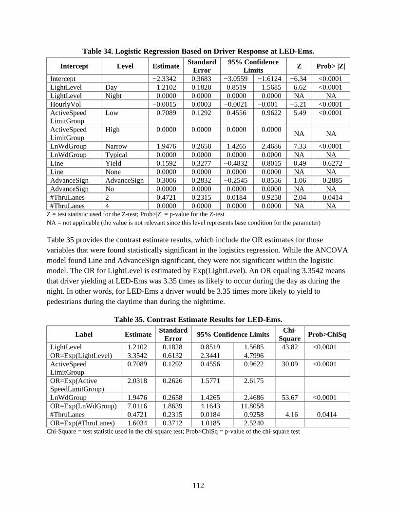
112

Table 34. Logistic Regression Based on Driver Response at LED-Ems.

Intercept Level Estimate Standard

Error

95% Confidence

Limits Z Prob> |Z|

Intercept −2.3342 0.3683 −3.0559 −1.6124 −6.34 <0.0001

LightLevel Day 1.2102 0.1828 0.8519 1.5685 6.62 <0.0001

LightLevel Night 0.0000 0.0000 0.0000 0.0000 NA NA

HourlyVol −0.0015 0.0003 −0.0021 −0.001 −5.21 <0.0001

ActiveSpeed

LimitGroup

Low 0.7089 0.1292 0.4556 0.9622 5.49 <0.0001

ActiveSpeed

LimitGroup

High 0.0000 0.0000 0.0000 0.0000 NA NA

LnWdGroup Narrow 1.9476 0.2658 1.4265 2.4686 7.33 <0.0001

LnWdGroup Typical 0.0000 0.0000 0.0000 0.0000 NA NA

Line Yield 0.1592 0.3277 −0.4832 0.8015 0.49 0.6272

Line None 0.0000 0.0000 0.0000 0.0000 NA NA

AdvanceSign AdvanceSign 0.3006 0.2832 −0.2545 0.8556 1.06 0.2885

AdvanceSign No 0.0000 0.0000 0.0000 0.0000 NA NA

#ThruLanes 2 0.4721 0.2315 0.0184 0.9258 2.04 0.0414

#ThruLanes 4 0.0000 0.0000 0.0000 0.0000 NA NA Z = test statistic used for the Z-test; Prob>|Z| = p-value for the Z-test


Table 35 provides the contrast estimate results, which include the OR estimates for those

variables that were found statistically significant in the logistics regression. While the ANCOVA

model found Line and AdvanceSign significant, they were not significant within the logistic

model. The OR for LightLevel is estimated by Exp(LightLevel). An OR equaling 3.3542 means

that driver yielding at LED-Ems was 3.35 times as likely to occur during the day as during the

night. In other words, for LED-Ems a driver would be 3.35 times more likely to yield to

pedestrians during the daytime than during the nighttime.

Table 35. Contrast Estimate Results for LED-Ems.

Label Estimate Standard

Error 95% Confidence Limits

Chi-

Square Prob>ChiSq

LightLevel 1.2102 0.1828 0.8519 1.5685 43.82 <0.0001

OR=Exp(LightLevel) 3.3542 0.6132 2.3441 4.7996

ActiveSpeed

LimitGroup

0.7089 0.1292 0.4556 0.9622 30.09 <0.0001

OR=Exp(Active

SpeedLimitGroup)

2.0318 0.2626 1.5771 2.6175

LnWdGroup 1.9476 0.2658 1.4265 2.4686 53.67 <0.0001

OR=Exp(LnWdGroup) 7.0116 1.8639 4.1643 11.8058

#ThruLanes 0.4721 0.2315 0.0184 0.9258 4.16 0.0414

OR=Exp(#ThruLanes) 1.6034 0.3712 1.0185 2.5240 Chi-Square = test statistic used in the chi-square test; Prob>ChiSq = p-value of the chi-square test

113

CONCLUSIONS

During this research effort, researchers collected about 224 hours of video that included

7871 drivers reacting to a staged pedestrian crossing. Researchers supplemented this dataset with

data from a recent research effort that included 48 hours of video and 1430 drivers. Therefore,

the analysis documented herein considered 9301 drivers for 3871 staged pedestrian crossings.

All evaluations clearly show that overall, the DYR was different for the three pedestrian

treatments studied, with the PHB having the highest yielding and the LED-Ems having the

lowest yielding. While overall there is a statistically significant difference between the treatment

types, there were sites where a treatment had a higher (or lower) yielding rate than the average

for the other treatments. For example, the LED-Em located on a college campus had a daytime

DYR of 84 percent, which is higher than the average RRFB DYR of 77 percent and is near the

maximum per-site DYR of 90 percent observed for any RRFB site.

The initial statistical evaluation that included interaction terms between treatment type and other

site characteristic variables found significant interaction effects as well as a significant difference

between treatment types. That evaluation also found the driver yielding effectiveness for a

treatment with respect to daytime and nighttime conditions varies for the different treatments,

which supported conducting evaluations separately for each treatment type.

For each treatment, two statistical evaluations were conducted: ANCOVA models that

considered per-site mean yield rates and logistic regression that considered the individual driver

response to the crossing pedestrian. Because of the nature of ANCOVA modeling, interpretation

of the results is easier; however, the logistic modeling provides the opportunity to use data for

individual drivers rather than a site average. Being able to use the data for each driver provides

the opportunity to consider individual responses rather than collapsing the variability into a site

average.

The statistical evaluations for the day and night effectiveness for the PHB found mixed results.

The ANCOVA model found a statistically significant difference, with daytime driver yielding

slightly higher, while the logistics regression did not find a statistically significant difference.

Even though the ANCOVA model found the PHB to be more effective during the day, the

difference was very small (98 percent during the day and 96 percent during the night) and may

not be of practical significance.

The analyses conducted for each treatment type also provided the opportunity to identify if there

are variables that are more influential for one treatment type than another. The PHB, with very

high driver yielding, did not have any site characteristics that were found to also influence driver

yielding.

114

The characteristics of the sites with RRFBs included in this analysis provided only limited

additional understanding of relationships. A previous study on the RRFB found higher driver

yielding at two-leg (midblock) sites, when a median refuge is present, when a school is within

0.5 miles of the crosswalk, and when yield lines are present. This study found that the light

conditions can influence driver yielding, with higher yielding at night. The presence of yield

lines as compared to no lines was also found to affect driver yielding although the difference was

only marginally significant.

This effort provided many insights into how crossing characteristics influence driver yielding at

sites with the LED-Em. Using the results from the logistic regression evaluation, higher driver

yielding was observed at LED-Em sites in the lower speed limit group (30 or 35 mph), with two

lanes (rather than four lanes), with narrow lanes of 10.5- or 11-ft widths (rather than 11.5- or

12-ft widths), and lower hourly volumes. The results from the ANCOVA model show a

statistically significant difference for yield lines (higher yielding when present) and suggest

higher driver yielding for sites with lower average hourly volumes, with narrow lanes, with

lower speed limit group (marginally significant), with two lanes (marginally significant), and

with an advance sign (marginally significant).

In summary, the focus of this research was to identify if the pedestrian treatment was effective at

night. For the PHB, essentially no difference was found between daytime and nighttime driver

yielding. The research found RRFBs to be more effective at night (statistically significant in both

ANCOVA and logistical regression evaluations) and the LED-Em to be more effective during

the day (statistically significant in both ANCOVA and logistical regression evaluations).

115

REFERENCES

1. Federal Highway Administration. Manual on Uniform Traffic Control Devices for Streets

and Highways: 2009 Edition Revised. U.S. Department of Transportation, Washington,

D.C., 2012.

2. Texas Department of Transportation. 2011 Texas Manual on Uniform Traffic Control

Devices: Revision 2. Austin, Texas, 2014.

3. Migletz, J., J. K. Fish, and J. L. Graham. Roadway Delineation Practices Handbook.

Report FHWA-SA-93-001. U.S. Department of Transportation, Federal Highway

Administration, Washington, D.C., 1994.

4. Grant, A. R., and J. R. Bloomfield. Guidelines for the Use of Raised Pavement Markers.

The University of Iowa, Iowa City, Iowa, 1998.

5. Zador, P., H. S. Stein, P. Wright, and J. Hall. Effects of Chevrons, Post-Mounted

Delineators, and Raised Pavement Markers on Driver Behavior at Roadway Curves.

Transportation Research Record: Journal of the Transportation Research Board, 1114,

Transportation Research Board of the National Academies, Washington, D.C., 1987,

pp. 1–10.

6. Bahar, G., C. Mollett, B. Persaud, C. Lyon, A. Smiley, T. Smahel, and H. McGee.

NCHRP Report 518: Safety Evaluation of Permanent Raised Pavement

Markers. National Cooperative Highway Research Program, Transportation Research

Board of the National Academies, Washington, D.C., 2004.

7. Niessner, C. W. Raised Pavement Markers at Hazardous Locations. Report FHWA-TS-

84-215. U.S. Department of Transportation, Federal Highway Administration,

Washington, D.C., 1984.

8. Blaauw, G. J. Vehicle Guidance by Delineation Systems at Night. Ergonomics, 28(12),

1985, pp. 1601–1615.

9. Zwahlen, H. T. Driver Lateral Control Performance as a Function of Delineation.

Transportation Research Record: Journal of the Transportation Research Board, 1149,

Transportation Research Board of the National Academies, Washington, D.C., 1987,

pp. 56–65.

10. Khan, M. M. Evaluation of Raised Pavement Markers at High Hazard Locations. Ohio

Department of Transportation, Division of Highways, Bureau of Traffic Control,

Columbus, Ohio, 1980.

11. Kugle, C. L., O. J. Pendleton, and M. Von Tress. An Evaluation of the Accident

Reduction Effectiveness of Raised Pavement Markers. Texas Transportation Institute,

College Station, Texas, 1984.

116

12. Mak, K. K., T. Chira-chavala, and L. I. Griffin. Evaluation of the Safety Effects of Raised

Pavement Markers. Texas Transportation Institute, College Station, Texas, 1987.

13. Pendleton, O. J. Evaluation of Accident Analysis Methodology. FHWA-RD-96-039. U.S.

Department of Transportation, Federal Highway Administration, Washington, D.C.,

1996.

14. Federal Highway Administration. National Roadway Safety Awards 2013 Noteworthy

Practices Guide. U.S. Department of Transportation, Washington, D.C., 2013.

15. Sun, X., and S. Das. Developing Louisiana Crash Reduction Factors. Department of

Civil and Environmental Engineering, University of Louisiana at Lafayette, Lafayette,

Louisiana, 2013.

16. Zwahlen, H. T., and T. Schnell. Visibility of New Pavement Markings at Night under

Low-Beam Illumination. Transportation Research Record: Journal of the Transportation

Research Board, 1495, Transportation Research Board of the National Academies,

Washington, D.C., 1995, pp. 117–127.

17. Zwahlen, H. T., and T. Schnell. Visibility of New Centerline and Edge Line Pavement

Markings. Transportation Research Record: Journal of the Transportation Research

Board, 1605, Transportation Research Board of the National Academies, Washington,

D.C., 1997, pp. 49–61.

18. Pike, A., and T. Barrette. Pavement Markings—Wet Retroreflectivity Standards. Report

MN 2020-09. Texas A&M Transportation Institute, College Station, Texas, 2020.

19. Ye, F., and A. Pike. Studying the Nighttime Visibility Performance of Retroreflective

Pavement Markers. Transportation Research Record: Journal of the Transportation


Washington, D.C., 2019, pp. 334–344.

20. Pike, A., T. Barrette, S. Hallmark, N. Oneyear, G. Basulto-Elias, O. Smadi, R.

Srinivasan, W. Kumfer, T. Saleem, F. Ye, P. Carlson, H.G. Hawkins, and T. Lindheimer.

NCHRP Project 05-21: Safety and Performance Criteria for Retroreflective Pavement

Markers. Research report under final review with the National Cooperative Highway

Research Program. Texas A&M Transportation Institute, College Station, Texas, 2019

(unpublished).

21. Bonneson, J., M. Pratt, J. Miles, and P. Carlson. Development of Guidelines for

Establishing Effective Curve Advisory Speeds. Report FHWA/TX-07/0-5439-1. Texas

A&M Transportation Institute, College Station, Texas, 2007.

22. Boodlal, L., E. Donnell, R. Porter, D. Garimella, T. Le, K. Croshaw, S. Himes, P. Kulis,

and J. Wood. Factors Influencing Operating Speeds and Safety on Rural and Suburban

Roads. Report FHWA-HRT-15-030. Federal Highway Administration, U.S. Department

of Transportation, Washington, D.C., 2015.

117

23. Arien, C., K. Brijs, G. Vanroelen, W. Ceulemans, E. Jongen, S. Daniels, T. Brijs, and G.

Wets. The Effect of Pavement Markings on Driving Behaviour in Curves: A Simulator

Study. Ergonomics, Vol. 60, No. 5, 2016, pp. 701–713.

24. Hallmark, S., N. Hawkins, and O. Smadi. Toolbox of Countermeasures for Rural Two-

Lane Curves. IHRB Project TR-579. Midwest Transportation Consortium, Ames, Iowa,

2013.

25. Frierson, T. Low-Cost Experimental Treatments for Horizontal Curves. Report TRC1305.

Arkansas State Highway and Transportation Department, Transportation Research

Committee, Little Rock, Arkansas, 2016.

26. Glennon, J. State of the Art Related to Safety Criteria for Highway Curve Design.

Research Report 134-4. Texas Transportation Institute, College Station, Texas, 1969.

27. Arnold, E., and K. Lantz. Evaluation of Best Practices in Traffic Operations and Safety:

Phase I: Flashing LED Stop Sign and Optical Speed Bars. Report FHWA/VTRC 07-R34.

Virginia Transportation Research Council, Charlottesville, Virginia, 2007.

28. Balde, A. Speed Management in Rural Communities Using Optical Speed Bars. Master

of science thesis, Kansas State University, Manhattan, Kansas, 2010.

29. Calvi, A. Investigating the Effectiveness of Perceptual Treatments on a Crest Vertical

Curve: A Driving Simulator Study. Transportation Research Part F, Vol. 58, 2018,

pp. 1074–1086.

30. Katz, B. Pavement Markings for Speed Reduction. Science Applications International

Corporation, McLean, Virginia, 2004.

31. Texas Department of Transportation. 2006 Texas Manual on Uniform Traffic Control

Devices. Austin, Texas, 2006.

32. Bonneson, J., M. Pratt, J. Miles, and P. Carlson. Procedures for Setting Advisory Speed:

Course Notes—Appendix A. Horizontal Curve Signing Handbook, 2nd Edition. Report

FHWA/TX-09/5-5439-01-P1. Texas A&M Transportation Institute, College Station,

Texas, 2009.

33. Glennon, J. Thoughts on a New Approach for Signing Roadway Curves.

http://www.crashforensics.com/papers.cfm?PaperID=18.

34. Torbic, D., D. Harwood, D. Gilmore, R. Pfefer, T. Neuman, K. Slack, and K. Hardy.

Guidance for Implementation of the AASHTO Strategic Highway Safety Plan. Volume 7:

A Guide for Reducing Collisions on Horizontal Curves. NCHRP Report 500.

Transportation Research Board, National Research Council, Washington, D.C., 2004.

35. Institute of Transportation Engineers and Federal Highway Administration. Engineering

Countermeasures to Reduce Red-Light Running (RLR). Issue Brief 6. 2004.

https://www.ite.org/pub/?id=e26c796b%2D2354%2Dd714%2D5117%2D125d2ad594bd.

http://www.crashforensics.com/papers.cfm?PaperID=18

https://www.ite.org/pub/?id=e26c796b%2D2354%2Dd714%2D5117%2D125d2ad594bd

118

36. Ringer, J., P. Koonce, J. Bansen, T. Nguyen, J. McGill, D. Stewart, J. Suggett, T.

Meuman, N. Antonucci, K. Hardy, and K. Courage. Signalized Intersections:

Informational Guide. Report No. FHWA-HRT-04-091. Federal Highway Administration,

U.S. Department of Transportation, Washington, D.C., August 2004.

37. Federal Highway Administration. Intersections Proven Safety Countermeasures.

Technical Summary: Backplates with Retroreflective Borders. Report No. FHWA-SA-15-

007. U.S. Department of Transportation, Washington, D.C., 2015.

https://safety.fhwa.dot.gov/intersection/conventional/signalized/backplates/tech/index.cf

m.

38. Federal Highway Administration. Proven Safety Countermeasures: Backplates with

Retroreflective Borders. Report No. FHWA-SA-17-051. U.S. Department of

Transportation, Washington, D.C., 2017.

https://safety.fhwa.dot.gov/provencountermeasures/blackplate/.

39. Miska, E., P. de Leur, and T. Sayed. Road Safety Performance Associated with Improved

Traffic Signal Design and Increased Signal Conspicuity. 2002 Compendium of Technical

Papers, Institute of Transportation Engineers, 72nd Annual Meeting, Philadelphia,

Pennsylvania, 2002.

40. Sayed, T., P. Leur, and J. Pump. Safety Impact of Increased Traffic Signal Backboards

Conspicuity. Transportation Research Board 84th Annual Meeting: Compendium of

Papers CD-ROM. Transportation Research Board of the National Academies,


41. Sayed, T., M. El Esawey, and J. Pump. Evaluating Impact on Safety of Improved Signal

Visibility at Urban Signalized Intersections. Transportation Research Record: Journal of

the Transportation Research Board, 2019, Transportation Research Board of the National

Academies, Washington D.C., 2007, pp. 51–56.

42. Agent, K. Low-Cost Safety Measures at Signalized Intersections. Research Report KTC-

08-11/SPR316-06-1F. Kentucky Transportation Center, University of Kentucky,

Lexington, Kentucky, May 2008.

43. Dissanayake, S., and I. Dias. Evaluation of Low-Cost Intersection Countermeasures to

Reduce Red-Light-Running Violations: Retro-Reflective Signal Back Plates. Report No.

25-1121-0003-165. Mid-America Transportation Center, Lincoln, Nebraska, November

2013.

44. Federal Highway Administration. Retroreflective Borders on Traffic Signal Backplates: A

South Carolina Success Story. Report No. FHWA-SA-09-11. U.S. Department of

Transportation, Washington, D.C., February 2010.

45. Sullivan, A., S. L. Jones, E. Tedla, and E. Doustmohammadi. Traffic Signal Design

Guide and Timing Manual. Alabama Department of Transportation, Montgomery,

Alabama, June 2015.

https://safety.fhwa.dot.gov/intersection/conventional/signalized/backplates/tech/index.cfm

https://safety.fhwa.dot.gov/intersection/conventional/signalized/backplates/tech/index.cfm

https://safety.fhwa.dot.gov/provencountermeasures/blackplate/

119

46. Florida Department of Transportation. Section 650—Vehicular Traffic Signal

Assemblies. Standard Specifications for Road and Bridge, Tallahassee, Florida, January

2020. https://fdotwww.blob.core.windows.net/sitefinity/docs/default-

source/programmanagement/implemented/specbooks/january-2020/1-20-

ebook.pdf?sfvrsn=e3eca19a_2.

47. Florida Department of Transportation. Section 232—Signalization. Design Manual,

Tallahassee, Florida, January 1, 2019.

48. Louisiana Department of Transportation and Development. Traffic Signal Manual.

Version 2.0. Baton Rouge, Louisiana, May 13, 2015.

49. Maine Department of Transportation. Maine DOT Mobility Report. Augusta, Maine,

November 2018.

50. Nevada Department of Transportation. Signal, Lighting, and ITS Design Guide. Carson

City, Nevada, 2019. https://www.nevadadot.com/home/showdocument?id=17155.

51. Nevada Department of Transportation. Standard Plans for Road and Bridge

Construction. Carson City, Nevada, 2020.

https://www.nevadadot.com/home/showdocument?id=17276.

52. Ohio Department of Transportation. Traffic Engineering Manual—Traffic Signals.

Columbus, Ohio, October 23, 2002.

http://www.dot.state.oh.us/Divisions/Engineering/Roadway/DesignStandards/traffic/TE

M/Documents/Part_04_Complete_01-16-15Revision_011315_bookmarked.pdf.

53. Ohio Department of Transportation. Construction and Material Specifications.

Columbus, Ohio, 2016.

http://www.dot.state.oh.us/Divisions/ConstructionMgt/OnlineDocs/Specifications/2016C

MS/2016_CMS_07192019_for_web_letter_size_with_SS800_Included.pdf.

54. R. N. Roman. Traffic Signal Backplate Standardization, Strike Off Letter. #494-17-01.

Bureau of Maintenance and Operations, Pennsylvania Department of Transportation,

Harrisburg, Pennsylvania, March 9, 2017.

55. Virginia Department of Transportation. High Visibility Signal Backplates. Instructional

and Informational Memorandum. Traffic Engineering Division, Richmond, Virginia,

April 22, 2018.

56. Washington State Department of Transportation. Chapter 1330. Washington State

Department of Transportation Design Manual, Olympia, Washington, September 2020.

https://www.wsdot.wa.gov/publications/manuals/fulltext/M22-01/1330.pdf.

57. Bretherton, W. M., and J. Miao. Proposed Guidelines for Traffic Actuated Warning Signs

at Intersections with Limited Sight Distance. Georgia Department of Transportation,

Atlanta, Georgia, 1996.

https://fdotwww.blob.core.windows.net/sitefinity/docs/default-source/programmanagement/implemented/specbooks/january-2020/1-20-ebook.pdf?sfvrsn=e3eca19a_2



https://www.nevadadot.com/home/showdocument?id=17155

https://www.nevadadot.com/home/showdocument?id=17276

http://www.dot.state.oh.us/Divisions/Engineering/Roadway/DesignStandards/traffic/TEM/Documents/Part_04_Complete_01-16-15Revision_011315_bookmarked.pdf

http://www.dot.state.oh.us/Divisions/Engineering/Roadway/DesignStandards/traffic/TEM/Documents/Part_04_Complete_01-16-15Revision_011315_bookmarked.pdf

http://www.dot.state.oh.us/Divisions/ConstructionMgt/OnlineDocs/Specifications/2016CMS/2016_CMS_07192019_for_web_letter_size_with_SS800_Included.pdf

http://www.dot.state.oh.us/Divisions/ConstructionMgt/OnlineDocs/Specifications/2016CMS/2016_CMS_07192019_for_web_letter_size_with_SS800_Included.pdf

https://www.wsdot.wa.gov/publications/manuals/fulltext/M22-01/1330.pdf

120

58. Kwon, T. M., and H. Ismail. Advanced LED Warning Systems for Rural Intersections:

Phase 2 (ALERT-2). Report No. MN/RC 2014-10. University of Minnesota Duluth,

Minnesota Department of Transportation, St. Paul, Minnesota, February 2014.

59. Kuehl, R., S. Petersen, J. Jackels, and M. Marti. Intersection Safety Technologies

Guidebook. Report No. MN/RC 2016RIC10. SRF Consulting Group, Inc., Minnesota

Department of Transportation, St. Paul, Minnesota, May 2016.

60. Himes, S., F. Gross, K. Eccles, and B. Persaud. Multistate Evaluation of Intersection

Conflict Warning Systems. FHWA-HRT-16-035. Federal Highway Administration, U.S.

Department of Transportation, Washington, D.C., June 2016.

61. American Standards Association, American Association of State Highway Officials, and

National Conference on Street and Highway Safety. Manual on Uniform Traffic Control

Devices. Washington, D.C., 1935.

62. American Association of State Highway Officials, Institute of Traffic Engineers, and

National Conference on Street and Highway Safety. Manual on Uniform Traffic Control

Devices. Washington, D.C., 1948.

63. American Association of State Highway Officials and National Joint Committee on

Uniform Traffic Control Devices. Manual on Uniform Traffic Control Devices. Federal

Highway Administration, U.S. Department of Transportation, Washington, D.C., 1971.

64. National Committee on Uniform Traffic Control Devices. NCUTCD Approved Changes

to the Manual on Uniform Traffic Control Devices. Pavement Marking Standards for

Automated Driving Systems and Improved Safety, Markings Committee, Item No. 19B-

MKG-02, January 2020. https://ncutcd.org/wp-content/uploads/meetings/2020A/04.19B-

MKG-02.LineWidthforCAV.pdf.

65. Abdel-Rahim, A., K. Chang, M. Mohamed, A. Skinner, and E. Kassem. Safety Impacts of

Using Wider Pavement Markings on Two-Lane Rural Highways in Idaho. Report

FHWA-ID-18-244. National Institute for Advanced Transportation Technology,

Moscow, Idaho, 2018.

66. McKnight, A. S., A. J. McKnight, and A. S. Tippetts. The Effect of Lane Line Width and

Contrast upon Lane Keeping. Accident Analysis and Prevention, 30(5), 1998, pp. 617–

624.

67. Charlton, S., and N. Starkey. Risk in Our Midst: Centrelines, Perceived Risk, and Speed

Choice. Accident Analysis and Prevention, 95, 2016, pp. 192–201.

68. Ward, A. Sighting Safety. Effectiveness of Highway Safety Improvements, American

Society of Civil Engineers, Reston, Virginia, 1985, pp. 61–72.

69. Carlson, P., E. S. Park, A. Pike, R. J. Porter, J. Miles, B. Boulanger, and A.

Burde. Pavement Marking Demonstration Projects: State of Alaska and State of

https://ncutcd.org/wp-content/uploads/meetings/2020A/04.19B-MKG-02.LineWidthforCAV.pdf

https://ncutcd.org/wp-content/uploads/meetings/2020A/04.19B-MKG-02.LineWidthforCAV.pdf

121

Tennessee. Report FHWA-HRT-12-048. Federal Highway Administration, U.S.

Department of Transportation, Washington, D.C., 2013.

70. Donnell, E., M. Gemar, and I Cruzado. Operational Effects of Wide Edge Lines Applied

to Horizontal Curves on Two-Lane Rural Highways. Report FHWA-PA-2006-006-

510401-04. Pennsylvania Transportation Institute, University Park, Pennsylvania, 2006.

71. Cottrell, B. The Effects of Wide Edge Lines on Lateral Placement and Speed on Two-

Lane Rural Roads. Transportation Research Record: Journal of the Transportation


Washington, D.C., 1986, pp. 1–6.

72. Miles, J., P. Carlson, R. Eurek, J. Re, and E.S. Park. Evaluation of Potential Benefits of

Wider and Brighter Edge Line Pavement Markings. Report FHWA/TX-10/0-5862-1.

Texas Transportation Institute, College Station, Texas, 2010.

73. Pike, A., and M. Manser. Pavement Marking Patterns and Widths-Human Factor Study.

Texas A&M Transportation Institute, College Station, Texas. Research in progress for the

Minnesota Department of Transportation, 2019–2021.

74. Pike, A., T. Barrette, and P. Carlson, P. Evaluation of the Effects of Pavement Marking

Width on Detectability by Machine Vision: 4-Inch vs. 6-Inch Markings. Prepared for the

American Traffic Safety Services Association. Texas A&M Transportation Institute,

College Station, Texas, 2018.

75. Fleming, K. Evaluation of Wider Edge Lines on Minnesota Roads. Minnesota

Department of Transportation, Office of Traffic, Safety, and Technology, St. Paul,

Minnesota, 2013.

76. Park, E. S., P. Carlson, R. J. Porter, and C. Andersen. Safety Effects of Wider Edge Lines

on Rural, Two-lane Highways. Accident Analysis and Prevention, 48, 2012, pp. 317–325.

77. Potts, I., D. Harwood, C. Bokenkroger, and M. Knoshaug. Benefit/Cost Evaluation of

MoDOT’s Total Striping and Delineation Program: Phase II. CM 12-002. Prepared for

the Missouri Department of Transportation. MRIGlobal, Kansas City, Missouri, 2011.

78. Hughes, W., H. McGee, S. Hussain, and J. Keegel. Field Evaluation of Edgeline Widths.

Bellomo-Mcgee, Inc., 1989.

79. Hall, J. Evaluation of Wide Edgelines (Discussion and Closure). Transportation

Research Record: Journal of the Transportation Research Board, 1114, Transportation

Research Board of the National Academies, Washington, D.C., 1987, pp. 21–30.

80. Cottrell, B. Evaluation of Wide Edgelines on Two-Lane Rural Roads. Report VTRC 87-

R23. Virginia Transportation Research Council, Charlottesville, Virginia, 1987.

81. Carlson, P., and J. Wagner. An Evaluation of the Effectiveness of Wider Edge Line

Pavement Markings. Texas Transportation Institute, College Station, Texas, 2012.

122

82. Ohme, P. Enhancing Nighttime Pavement Marking Visibility for Older Drivers. Doctoral

dissertation, University of Iowa, Ames, Iowa, 2001.

83. Pietrucha, M. T., R. S. Hostetter, L. Staplin, and M. Obermeyer. Pavement Markings and

Delineation for Older Drivers. Final Report. Report FHWA-RD-94-145. Pennsylvania

Transportation Institute, University Park, Pennsylvania, 1996.

84. Gibbons, R. B., B. Williams, and B. Cottrell. Assessment of Durability of Wet Night

Visible Pavement Markings: Visibility Experiment. Transportation Research Record:

Journal of the Transportation Research Board, 2337, Transportation Research Board of

the National Academies, Washington, D.C., 2013, pp. 67–73.

85. European Cooperation in the Field of Scientific, Technical Research (Organization), and

European Commission Directorate-General Transport. COST 331: Requirements for

Horizontal Road Marking: Final Report of the Action (Vol. 1). Office for Official

Publications of the European Communities, 1999.

86. Gibbons, R. B., M. J. McElheny, and C. J. Edwards. Impact of Pavement Marking Width

on Visibility Distance. No. 06-1859. TRB 85th Annual Meeting Compendium of Papers

CD-ROM, Transportation Research Board of the National Academies, Washington, D.C.,

2006.

87. Gibbons, R. B. Pavement Marking Visibility Requirements during Wet Night Conditions.

Virginia Center for Transportation Innovation and Research, Blacksburg, Virginia, 2006.

88. Carlson, P., J. Miles, A. Pike, and E. S. Park. Evaluation of Wet-Weather and Contrast

Pavement Marking Applications: Final Report. Texas Transportation Institute, College

Station, Texas, 2007.

89. Carlson, P., E. S. Park, C. Andersen, B. Kuhn, A. Pike, J. Miles, and R. J.

Porter. Pavement Marking Demonstration Project: State of Alaska and State of

Tennessee-Report to Congress. Report FHWA-HRT-09-039. U.S. Department of

Transportation, Federal Highway Administration, Washington D.C., 2010.

90. Zwahlen, H., and T. Schnell. Visibility of New Pavement Markings at Night under Low-

Beam Illumination. Transportation Research Record: Journal of the Transportation


Washington, D.C., 1995, pp. 117–127.

91. Pike, A., and T. Barrette. Pavement Markings—Wet Retroreflectivity Standards. Report

No. 2020-09. Prepared for the Minnesota Department of Transportation. Texas A&M

Transportation Institute, College Station, Texas 2020.

92. Gates, T., and H. G. Hawkins. The Use of Wider Longitudinal Pavement Markings.

Research Report 0024-1. Texas Transportation Institute, College Station, Texas, 2002.

93. Obeng-Boampong, K., A. Pike, J. Miles, and P. Carlson. Use of Wider Pavement

Markings—Survey of State Transportation Agencies. Paper Number 09-1113. TRB 88th

123

Annual Meeting Compendium of Papers DVD, Transportation Research Board of the

National Academies, Washington, D.C., 2009.

94. Pike, A., and B. Bommanayakanahalli. Development of a Pavement Marking Life Cycle

Cost Tool. Paper Number 18-1533. 2018 Annual Transportation Research Board

Meeting Compendium of Papers, Transportation Research Board of the National

Academies, Washington, D.C., 2018.

95. Moran, M. J., and C. Monje. Memorandum re: Guidance on Treatment of the Economic

Value of a Statistical Life (VSL) in U.S. Department of Transportation Analyses—2016

Adjustment. August 8, 2016.

96. Texas Department of Transportation. Barricade and Construction (BC) Project Limit

Standard Sheet BC (2)-14. Austin, Texas, August 2014.

http://www.dot.state.tx.us/insdtdot/orgchart/cmd/cserve/standard/toc.htm.

97. Texas Department of Transportation. Traffic Control Plan Standards. Austin, Texas.

https://www.dot.state.tx.us/insdtdot/orgchart/cmd/cserve/standard/toc.htm.

98. Texas Department of Public Safety. Texas Driver Handbook. Driver License Division,

Austin, Texas, September 2017. https://www.dps.texas.gov/internetforms/Forms/DL-

7.pdf.

99. Texas Department of Transportation. Cell Phone Ordinances. Austin, Texas.

https://www.txdot.gov/inside-

txdot/division/traffic/safety/laws/cellphones.html#:~:text=Cellphone%20laws%20to%20r

emember,a%20school%20zone%20is%20illegal.

100. Texas Department of Transportation. Standard Highway Sign Designs. 2012 edition,

revision 2. Austin, Texas, March 2017. http://ftp.dot.state.tx.us/pub/txdot-info/trf/shsd-

2012-complete_060512.pdf.

101. Texas Department of Transportation. Barricade and Construction (BC) Temporary Sign

Notes Standard Sheet BC (4)-14. Austin, Texas, August 2014.

http://www.dot.state.tx.us/insdtdot/orgchart/cmd/cserve/standard/toc.htm.

102. Texas Department of Transportation. Smart Work Zone Guidelines: Design Guidelines

for Deployment of Work Zone Intelligent Transportation Systems (ITS). Austin, Texas,

October 2018. http://ftp.dot.state.tx.us/pub/txdot-info/trf/smart-work-zone-guidelines.pdf.

103. American Road and Transportation Builders Association. Designing Work Space Access

Points to Better Accommodate Large Trucks. Washington, D.C., 2020.

https://www.workzonesafety.org/files/documents/training/fhwa_wz_grant/artba_large_tru

ck_work_space_access_points_factsheet-508.pdf.

104. Texas Strategic Highway Safety Plan. Pedestrian Safety, Texas Strategic Highway Safety

Plan. 2020. https://www.texasshsp.com/emphasis-areas/pedestrian-safety/.

http://www.dot.state.tx.us/insdtdot/orgchart/cmd/cserve/standard/toc.htm

https://www.dot.state.tx.us/insdtdot/orgchart/cmd/cserve/standard/toc.htm

https://www.dps.texas.gov/internetforms/Forms/DL-7.pdf

https://www.dps.texas.gov/internetforms/Forms/DL-7.pdf

https://www.txdot.gov/inside-txdot/division/traffic/safety/laws/cellphones.html#:~:text=Cellphone%20laws%20to%20remember,a%20school%20zone%20is%20illegal



http://ftp.dot.state.tx.us/pub/txdot-info/trf/shsd-2012-complete_060512.pdf

http://ftp.dot.state.tx.us/pub/txdot-info/trf/shsd-2012-complete_060512.pdf

http://www.dot.state.tx.us/insdtdot/orgchart/cmd/cserve/standard/toc.htm

http://ftp.dot.state.tx.us/pub/txdot-info/trf/smart-work-zone-guidelines.pdf

https://www.workzonesafety.org/files/documents/training/fhwa_wz_grant/artba_large_truck_work_space_access_points_factsheet-508.pdf

https://www.workzonesafety.org/files/documents/training/fhwa_wz_grant/artba_large_truck_work_space_access_points_factsheet-508.pdf

https://www.texasshsp.com/emphasis-areas/pedestrian-safety/

124

105. Finley, M. D., K. Fitzpatrick, E. Rista, M.A. Brewer, R. Avelar, A. M. Pike, T. P.

Barrette, and S. Datta. Traffic Control Device Analysis, Testing, and Evaluation Program

FY2019 Activities. FHWA/TX-19/0-6969-R2. Texas A&M Transportation Institute,

College Station, Texas, October 2020.

https://static.tti.tamu.edu/tti.tamu.edu/documents/0-6969-R2.pdf.

106. Rista, E., and K. Fitzpatrick. Comparison of LED-Embedded Pedestrian Crossing Signs

to RRFBs and PHBs. Transportation Research Record: Journal of the Transportation

Research Board, Transportation Research Board of the National Academies, Washington,

D.C., September 16, 2020. https://doi.org/10.1177/0361198120941849.

107. Fitzpatrick, K., S. Turner, M. Brewer, P. Carlson, N. Lalani, B. Ullman, N. Trout, E. S.

Park, D. Lord, and J. Whitacre. Improving Pedestrian Safety at Unsignalized Crossings.

TCRP Report 112/NCHRP Report 562. Transportation Research Board of the National

Academies, Washington, D.C., 2006.

108. Turner, S., K. Fitzpatrick, M. Brewer, and E. S. Park. Motorist Yielding to Pedestrians at

Unsignalized Intersections Findings from a National Study on Improving Pedestrian

Safety. Transportation Research Record: Journal of the Transportation Research Board,

1982, Transportation Research Board of the National Academies, Washington, D.C.,

2006, pp. 1–12.

109. Fitzpatrick, K., R. Avelar, M. Pratt, M. Brewer, J. Robertson, T. Lindheimer, and J.

Miles. Evaluation of Pedestrian Hybrid Beacon and Rapid Flashing Beacons. Publication

HRT-16-040. Federal Highway Administration, U.S. Department of Transportation,


110. Fitzpatrick, K., and M. Pratt. Road User Behaviors at Pedestrian Hybrid Beacons.

Publication FHWA-HRT-16-039. Federal Highway Administration, U.S. Department of

Transportation, Washington, D.C., 2016.

111. Fitzpatrick, K., M. Cynecki, M. Pratt, E. S. Park, and M. Beckley. Evaluation of

Pedestrian Hybrid Beacons on Arizona Highways. Arizona Department of

Transportation, Phoenix, Arizona, 2019 (forthcoming).

112. Fitzpatrick, K., M. Brewer, R. Avelar, and T. Lindheimer. Will You Stop for Me?

Roadway Design and Traffic Control Device Influences on Drivers Yielding to

Pedestrians in a Crosswalk with a Rectangular Rapid-Flashing Beacon. Publication TTI-

CTS-0010. Texas A&M Transportation Institute, College Station, Texas, June 2016.

113. Hawkins, N., and B. A. Bektas. Evaluating the Effectiveness of the City of Des Moines

LED and RRFB Pedestrian Crossing Treatments on Multi-lane Roadways. Publication

Intrans 10-387. Iowa Department of Transportation, Ames, Iowa, December 2012.

114. Ellis, W., and J. P. Tremblay. Evaluation of BlinkerSign® Crosswalk Lighting System.

Publication 2014-13. Federal Highway Administration, U.S. Department of

Transportation, Washington, D.C., December 2014.

https://static.tti.tamu.edu/tti.tamu.edu/documents/0-6969-R2.pdf

https://doi.org/10.1177%2F0361198120941849

125

115. Hourdos, J. Assessing the Impact of Pedestrian-Activated Crossing Systems. Publication

CTS# 2016031. Minnesota Department of Transportation, St. Paul, Minnesota, July 2018.

116. Fitzpatrick K., V. Iragavarapu, M. Brewer, D. Lord, J. Hudson, R. Avelar, and J.

Robertson. Characteristics of Texas Pedestrian Crashes and Evaluation of Driver

Yielding at Pedestrian Treatments. Report FHWA/TX-14/0-6702-1. Texas A&M

Transportation Instiute, College Station, Texas, 2013.