traffic analysis of existing traffic in kulyab region in order to plan
TRANSCRIPT
Degree project inCommunication Systems
Second level, 30.0 HECStockholm, Sweden
I S A B E L F R O S T N E
Traffic analysis of existing trafficin Kulyab region in order to planand configure a new GSM MSC
for this region
K T H I n f o r m a t i o n a n d
C o m m u n i c a t i o n T e c h n o l o g y

i
Traffic analysis of existing traffic in Kulyab region in
order to plan and configure a new GSM MSC for this region
(Trafikanalys av existerande trafik i Kulyab-regionen inför planering och konfigurering av en ny GSM MSC för denna
region)
Isabel Frostne
2011.07.15
Supervisor in Industry: Vladimir Shlyshkov Employer: Babilon Mobile
Supervisor and Examiner: Prof. Gerald Q. Maguire Jr.
Royal Institute of Technology School of Information and Communication Technology
Stockholm, Sweden


i
Abstract Wide area cellular mobile networks have rapidly evolved over the years. In
the beginning achieving wide area coverage was a great achievement – enabling subscribers to call from wherever they were currently located and whenever they wanted. Additionally these systems supported mobility of subscribers, so that calls could continue even while a subscriber moved from one cell to another. Today mobility management is something everyone takes for granted. New functionality is continuously being developed for these networks. An important aspect of this evolution has been to enable new applications and technologies to be introduced while maintaining interoperability with the existing technologies.
These mobile networks use new technologies and enable new applications, but they interconnect with existing networks that utilize earlier technologies, such as the existing fixed telephone network. These interconnections enable communication between subscribers connected via all of these networks. In today’s mobile networks there are a variety of technologies working side by side, for example 2G, GPRS, 3G, and so on. The earlier networks used circuit switching technology, but the trend in later networks was to transition exclusively to packet switching.
One of the most important network entities is the mobile switch center (MSC). In the earlier circuit switched networks the MSC is the heart of the circuit switching network. The MSC is responsible for management, control, and communication to and from the mobile stations (MSs) in the area managed by the MSC. The MSC stores information about each of the MSs in one or more databases. In the subscriber’s home network the information about their subscription is stored in a home location register (HLR), while when this subscriber is in another network information is stored in a visitor location register (VLR). The MSC together with other elements of the core network handles mobility management, enabling both handover and roaming. A gateway MSC enables MSs to communicate with phones connected to the fixed network.
The aim of this thesis is to analyze the traffic situation for Kulyab region in order to configure and install the MSC in Kulyab. For the time being there is no radio network controller (RNC) in Kulyab region, so the MSC in Kulyab will be configured to support 2G traffic.
The configuration will be based on the expected mobile traffic load in the Kulyab region, thus the first steps in the process were to collect and analyze data about the existing traffic in this region that is currently served by a MSC located outside of this region. The configuration of the new MSC will be based on this analysis.
After installing and configuring the new MSC some question need to be answered, namely:

ii
1. Can the MSC in Kulyab support all the base stations in Kulyab region? If not, how many base stations can it support?
2. To what extent does the addition of this new MSC improve the overall network in terms of increased reliability, capacity, and throughput?
3. How much will the capacity of the existing MSC, that is responsible for traffic outside Dushanbe, be increased due to the introduction of the new MSC?

iii
Sammanfattning Den mobila täckningen har utvecklats snabbt under åren. Att uppnå den
mobila täckningen var i början en stor prestation – att kunna erbjuda telefontjänster för abonnenterna var än de befann sig och när de ville. Förutom detta så stödde detta system också fri rörlighet för abonnenterna. Under ett samtal kunde de förflytta sig från en cell till ett annan utan att samtalet bröts. Nu är mobilitetshanteringen någonting självklart. Nya funktioner utvecklas ständigt för dessa nätverk. En viktig aspekt för utvecklingen är att möjliggöra så att nya applikationer och teknologier kan introduceras och fortfarande vara kompatibla med de existerande teknikerna.
Dessa mobilnätverk använder nya tekniker och möjliggör nya applikationer som är kompatibla med det existerande nätverket. Det existerande nätverket använder sig av tidigare teknologier, så som den fasta telefonnätet. Detta möjliggör kommunikation mellan abonnenterna från olika nätverk. I dagens nätverk finns det ett antal olika nätverk, som t.ex. 2G, GPRS, 3G och så vidare. Det tidigare nätverket använde sig av kretskopplad teknik, men trenden är att uteslutande använda sig av paketkopplad teknik.
En av de viktigaste nätverksenheterna är ”Mobile switch center” (MSC). I de tidigare kretskopplade nätverket är MSC hjärtat i det kretskopplade nätverket. MSC är ansvarig för hanteringen, kontrollen och kommunikation till och från de mobila enheterna (MS) i området som kontrolleras av MSCn. MSC lagrar information om var och en av MS i ett eller flera databaser. I abonnentens hemnätverk finns information om abonnentens abonnemang i ett hemregister (HLR). När abonnenten befinner sig i ett annat nätverk lagras informationen i ett gästregister (VLR). MSC hanterar mobilitet tillsammans med andra nätverksenheter i ”Core network” (CN) och möjliggör överlämnande (handover) och roaming. ”Gateway MSC” GMSC möjliggör kommunikation mellan MS och det fasta nätverket.
Syftet med examensarbetet är att analysera trafiken för Kulyab-regionen för att konfigurera och installera en MSC i Kulyab. För tillfället finns ingen ”Radio network controller” (RNC) i regionen Kulyab, så MSCn i Kulyab kommer att konfigureras för att stödja 2G trafik.
Konfigurationen baseras på den förväntade belastningen av mobiltrafiken i Kulyab-regionen, följaktligen är det första steget i processen att samla ihop och analysera information om den existerande trafiken i Kulyab-regionen. Trafiken tillhörande Kulyab-regionen handskas för närvarande av en MSC som befinner sig utanför detta område. Konfigurationen av den nya MSCn kommer att baseras på denna analys.
Efter installationen och konfigurationen av den nya MSCn kommer följande frågor att bli besvarade, nämligen:
1. Kan MSCn i Kulyab stödja alla basstationerna i Kulyab regionen? Om inte, hur många basstationer kan MSCn stödja?
2. Till vilken grad kommer den nya MSCn att förbättra nätverket i termer av ökad tillförlitlighet, kapacitet och trafikgenomströmning?

iv
3. Hur mycket kommer kapacitetsökningen för den existerande MSC utanför Dushanbe att öka då MSC i Kulyab installeras?

v
Acknowledgements Firstly I would thank Babilon Mobile for giving me the opportunity to do
my thesis work in the company. All the co-workers were very supportive and helpful. Thank you very much. Special thanks go to Abdushukurov Rashid Khamidovich, Petrov Vasiliy Sergeevich, Saidov Mansur, Mirojov Azam, and to my supervisor Shlichkov Vladimir Vladimirovich. Thank you very much.
I would also like to thank my academic supervisor and examiner Professor Gerard Q. Maguire Jr. for the support, helpfulness and good advices throughout my thesis project. Thank you very much.


vii
Table of contents
Contents Abstract .............................................................................................................................. i Sammanfattning ............................................................................................................... iii Acknowledgements ........................................................................................................... v Table of contents ............................................................................................................. vii List of Figures .................................................................................................................. xi List of Tables ................................................................................................................. xiii List of Graphs ................................................................................................................ xvi List of Equations ............................................................................................................ xvi 1. Introduction ............................................................................................... 1
1.1. General Overview ..................................................................................... 1 1.1.1. Problem statement ..................................................................................... 2 1.1.2. Prior work .................................................................................................. 3 1.1.3. The Reader ................................................................................................ 3
1.2. A brief introduction to mobile networks that have evolved from GSM ... 3 1.2.1. Global System for Mobile Communication (GSM) .................................. 4 1.2.2. General Packet Radio Service (GPRS) ..................................................... 4 1.2.3. Universal Mobile Telecommunications System (UMTS) ......................... 4
1.3. Mobile Network System Architecture ...................................................... 6 1.3.1. Mobile Subscriber ..................................................................................... 6 1.3.2. Fixed networks .......................................................................................... 7
1.4. Entities in the core network ....................................................................... 8 1.4.1. HLR database ............................................................................................ 8 1.4.2. Operation and Network Management Centre ........................................... 9 1.4.3. Signaling Gateway (SG) ........................................................................... 9
1.5. Mobile Switching Center .......................................................................... 9 1.5.1. Detailed information about the MSC’s tasks .......................................... 10 1.5.2. The architecture of the MSC ................................................................... 11
1.6. Channel organization .............................................................................. 13 1.6.1. Switching performed in MSC server ....................................................... 14 1.6.2. The intelligent network ........................................................................... 14
1.7. How calls are switched ............................................................................ 16 1.8. Protocols used in the network ................................................................. 17
1.8.1. ATM (Asynchronous mode) ................................................................... 17 1.8.2. SS7 (Signaling system 7) ........................................................................ 18 1.8.3. SIGTRAN ............................................................................................... 20 1.8.4. H.248 ....................................................................................................... 21

viii
1.9. MSC configuration .................................................................................. 21 1.9.1. MSOFT ................................................................................................... 22 1.9.2. MSOFT hardware .................................................................................... 23 1.9.3. Software structure ................................................................................... 27 1.9.4. Signaling path .......................................................................................... 28 1.9.5. UMG8900 ............................................................................................... 28
1.10. Analyzing method for mobile traffic ....................................................... 35 1.10.1. The parameters used in analyzing quality of traffic ................................ 35 1.10.2. Traffic flow ............................................................................................. 37 1.10.3. Planning ................................................................................................... 39
2. Collection of statistic ............................................................................... 41 2.1. Calculation of the maximum capacity of the MSC as configured .......... 42 2.2. Calculation of the traffic statistics ........................................................... 43
2.2.1. Relative values ........................................................................................ 43 2.2.2. Calculation of the BHCA ........................................................................ 44 2.2.3. Calculation of traffic load in Erlangs ...................................................... 49 2.2.4. Calculating the average call duration ...................................................... 51
2.3. Analyzing strategy .................................................................................. 51 2.3.1. Analysis of the traffic in Kulyab ............................................................. 51 2.3.2. Analysis of the capacity gain for MSC-RRP .......................................... 52
3. Analysis of the collected statistics and the maximum capacity of the MSC .................................................................................................. 53
3.1. Calculation and analysis of the MSC server and MGW hardware capacities in Kulyab .................................................................................................... 53
3.1.1. The MSC server in Kulyab ..................................................................... 53 3.1.2. The MGW in Kulyab .............................................................................. 56
3.2. Analysis of traffic flows in Kulyab area ................................................. 56 3.2.1. The evaluation process ............................................................................ 57 3.2.2. Statistical analysis for the whole period (23rd of February to 25th
of March 2011) ........................................................................................ 58 3.2.3. Comparison of traffic on the 22nd and 23rd of March 2011 .................. 60 3.2.4. Day by day statistics ................................................................................ 67 3.2.5. Different peaks in time for BHCA and connect traffic in the same
day ........................................................................................................... 78 3.2.6. More analysis regarding average call duration ....................................... 89 3.2.7. Comparison of the maximum capacity of the MSC in Kulyab as
configured with the statistics collected from the base stations in Kulyab ..................................................................................................... 95
3.3. Efficiency analysis for the MSC-RRP .................................................... 98 3.3.1. Calculation of the hardware capacity in MSC-RRP ............................... 98 3.3.2. Analyzing the Kulyab traffic in the MSC-RRP ...................................... 99 3.3.3. Analysis of the traffic on the 17th of May 2011 ................................... 103
3.4. Analysis and proposed solutions ........................................................... 107

ix
3.4.1. Analysis of the Kulyab traffic ............................................................... 108 3.4.2. Proposed solution .................................................................................. 111
4. Configuration of the MSC in Kulyab .................................................... 113 4.1. Configuring the MSC server ................................................................. 113
4.1.1. Step 1: Configuration of the basic data ................................................. 114 4.1.2. Step 2: Configuring the interworking data ............................................ 114 4.1.3. Step 3: Configuring basic service data .................................................. 115
4.2. Configuring the MGW .......................................................................... 116 5. Conclusions and Future Work ............................................................... 117
5.1. Conclusions ........................................................................................... 117 5.2. Future work ........................................................................................... 118
References ..................................................................................................................... 121 Internet resources .......................................................................................................... 123 Appendix ....................................................................................................................... 125 A. MSOFT interfaces ................................................................................. 125 B. Call set-up flow diagram ....................................................................... 127 C. Measurement entities used in the statistics ........................................... 129 C.I Measurement entities for Kulyab traffic ............................................... 129 C.II Measurement entities for Kulyab traffic ............................................... 130 C.III Measurement entities for MSC-RRP .................................................... 131 D. Base stations analyzed for Kulyab region ............................................. 133 E. Relative BHCA values .......................................................................... 135 F. Relative values of the connect traffic .................................................... 139 G. Comparison of the traffic on the 22nd and 23rd March 2011 ............... 143 H. The traffic measured the 23rd of February ........................................... 145 I. Comparison of relative connected times and relative connected
traffic measured the 23rd of February 2011 ......................................... 147 J. Maximum values for relative BHCA and relative connected traffic .... 149 K. The hour when there is a peak ............................................................... 151 L. Percentage of Kulyab BHCA traffic for the MSC server in Kulyab ..... 153 M. Percentage of connected and response traffic load for the MGW in
Kulyab ................................................................................................... 157 N. Kulyab traffic the 17th of May 2011 ..................................................... 161 O. Calculation of the capacity increase for MSC-RRP .............................. 163 P. The ratio between connect times and seizure times for outgoing
trunk group the 21st of March 2011 ..................................................... 175 Q. Configuration example of equipment data ............................................ 181 R. Configuration example for local office data ......................................... 183 S. Average call duration calculated for the measurement period 23rd of February to 25th of March 20011 ............................................................................. 185 T. Maximum average call duration and the total average call duration for the measurement period of 23rd of February to the 25th of March ........................ 189

x
xi
List of Figures Figure 1: 3GPP architecture (Slide 306 of [45]. Appears with permission of
G.Q.Maguire Jr.). ...................................................................................... 5 Figure 2: The division of the core network into circuit switching and packet
switching. .................................................................................................. 5 Figure 3: States of the mobile station (MS) and their relationship ......................... 10 Figure 4: The MSC server is responsible for the control plane and the MGW
is responsible for the user plane. ............................................................. 12 Figure 5: The 32 time slots in TDMA. ................................................................... 13 Figure 6: Each speech channel is identified by a circuit identification code
(CIC) that identifies which timeslot (TS) that particular call is transmitted in. .......................................................................................... 14
Figure 7: The associated mode of operation. .......................................................... 15 Figure 8: The quasi-associated mode of operation. ................................................ 15 Figure 9: Speech and control signaling flows between two nodes in a SS7
system ...................................................................................................... 19 Figure 10: The path of the M2UA messages. ........................................................... 21 Figure 11: Some of the interfaces of the MSC server (MSOFTX3000) ................... 22 Figure 12: MSC is composed of MSOFTX3000 and UMG8900. The A-
interface connects the MSC to the base stations (GERAN) and Iu-interface connects the MSC with the node Bs (UTRAN). ...................... 23
Figure 13: The placement of the board in frame 1 of the Kulyab MSC server. ....... 24 Figure 14: The UMG communicates with the NEs through interfaces. ................... 29 Figure 15: Self-cascading in the MGW of Kulyab with six frames. Where the
dashed line GE indicates Gigabit Ethernet service data plane links and the solid line FE indicates Fast Ethernet service control planes. ..... 32
Figure 16: Traffic intensity (i.e. channel occupying) ............................................... 37 Figure 17: The measurement points for seizure times and connect times. ............... 45 Figure 18: Measurement points for early release times and seizure times. .............. 46 Figure 19: The relative seizure times, the relative connect times and their ratio
for fixed phones in Kulyab on the 26th of March 2011. ......................... 47 Figure 20: When the parameter 2G originating call attempts and MO try call
attempts are measured ............................................................................. 48 Figure 21: The measure points for 2G terminated call attempt and MT
Connect times .......................................................................................... 49 Figure 22: Measurement points for 2G MO seize usage and MO connect
traffic ....................................................................................................... 50 Figure 23: The MSC in Kulyab and the interworking network entities. The
dotted lines in the figure above depict control signaling and the solid lines are voice bearers. ................................................................. 113
Figure 24: ISUP messages sent when a call is setup (the figure is adapted from [27]) ....................................................................................................... 128


xiii
List of Tables Table 1: The placement of the front boards in the MSC server in Kulyab.
“H” stands for “having” that type of board. The symbol, “-“, stands for not having that type of board. ............................................................ 26
Table 2: Shows the placement of the back boards in the MSC server in Kulyab. .................................................................................................... 26
Table 3: Boards and their corresponding application software ............................. 27 Table 4: The boards corresponding to a specific module in the UMG ................. 31 Table 5: Shows the placement of the front boards in MGW Kulyab. “H”
stands for “having” that type of board. The symbol, “-“, stands for not having that type of board. ................................................................. 33
Table 6: Shows the placement of the back boards in MGW Kulyab. ................... 33 Table 7: Displays the unit and the corresponding boards for each board used
in the MGW of Kulyab. .......................................................................... 34 Table 8: The quality parameters with their target values ...................................... 36 Table 9: RXQUAL parameter ranges based upon BER before channel
decoding, adapted from table in section 8.2.4 on page 22 of [22] .......... 36 Table 10: Erlang B for blocking probabilities of 1, 2, 3, 5, and 10%, adapted
from table 2.13 in section 2.6.1 of [5]. .................................................... 38 Table 11: The capacity of the MSC server according to the number of
WCSUs and WCCUs (Note that the BHCA is a relative value. The relative BHCA value has been related to the highest BHCA value measured in the period 23rd of February to the 25th of March 2011) ....................................................................................................... 54
Table 12: Capacity of WEPI, WIFM, and WBSG .................................................... 55 Table 13: Capacity of the WCDB and WVDB boards ............................................ 55 Table 14: Total number of E1 for the MGW in Kulyab .......................................... 56 Table 15: Comparison of the highest values between BHCA and connected
traffic on the 22nd and 23rd March 2011.The highest measured values are highlighted. ............................................................................ 61
Table 16: Maximum value of BHCA and the maximum value of connect and response traffic occurs at different hours the 23rd of February 2011 ..... 71
Table 17: Maximum peak difference in time .......................................................... 78 Table 18: Maximum peaks within one hour ............................................................ 79 Table 19: Comparison of the collected BHCA statistics with the capacity of
the MSC server in Kulyab ....................................................................... 96 Table 20: Comparison of the collected traffic intensity with the capacity of the
MGW in Kulyab ...................................................................................... 97 Table 21: The capacity for the RRP MSC server in relative numbers .................... 98 Table 22: Relative BHCA traffic belonging to Kulyab region in the MSC-
RRP ....................................................................................................... 100 Table 23: Connect traffic belonging to Kulyab in the MSC-RRP ........................ 102

xiv
Table 24: Relative percentage of Kulyab traffic when there is a peak in the Kulyab traffic load ................................................................................ 103
Table 25: Traffic for the Kulyab traffic in the 17th of May 2011 ......................... 104 Table 26: Capacity gain for the MSC-RRP ........................................................... 107 Table 27: Tasks managed by a VMSC [3] ............................................................ 115 Table 28: Table of interfaces to/from the MSOFT switch .................................... 125 Table 29: Measurement entities for the statistics collected from base stations
in Kulyab region. The highlighted fields are those fields used in the analysis .................................................................................................. 130
Table 30: Measurement entities for the statistics collected from all base stations in MSC-RRP. The highlighted fields are those fields used in the analysis ........................................................................................ 131
Table 31: Cells located in LAC 0050 and 0051 .................................................... 133 Table 32: Relative BHCA values collected from the 23rd of February to 1st
of March 2011. The highest relative BHCA values are highlighted. The unit of BHCA is “call attempts” .................................................... 135
Table 33: Relative BHCA values collected from the 4th of February to 10th of March 2011 ....................................................................................... 136
Table 34: Relative BHCA values collected from the 11th of March to 15th of March 2011 ........................................................................................... 137
Table 35: Relative BHCA values collected from the 18th of March to 25th of March 2011 ........................................................................................... 138
Table 36: Values of the relative connected traffic collected from the 23rd of February to 1st of March 2011 .............................................................. 139
Table 37: Values of the relative connected traffic collected from the 4th of March to 10th of March 2011 ............................................................... 140
Table 38: Values of the relative connected traffic collected from the 11th of March to 15th of March 2011 ............................................................... 141
Table 39: Values of the relative connect traffic collected from the 18th of March to 25th of March 2011 ............................................................... 142
Table 40: Comparison of the relative BHCA and relative connected traffic on the 22nd and 23rd of March 2011 ......................................................... 143
Table 41: Traffic load the 23rd of February 2011 ................................................. 145 Table 42: Comparison of relative connected times and relative connected
traffic ..................................................................................................... 147 Table 43: Maximum values for relative BHCA and relative connected traffic
in Kulyab ............................................................................................... 149 Table 44: Hour when the daily peaks take place ................................................... 151 Table 45: Percentage of Kulyab BHCA traffic for the MSC server in Kulyab ..... 153 Table 46: Percentage of connected and response traffic load for the MGW in
Kulyab. Response traffic that has a maximum peak at a different time than the connected traffic is not displayed in the table ................. 157
Table 47: Highest measured values for the period 16th of May to 22nd of May 2011 .............................................................................................. 161
Table 48: Average call duration from 23rd of February to 1st of March 2011 ..... 185 Table 49: Average call duration from the 4th of March to 10th of March 2011 ... 186
xv
Table 50: Average call duration from the 11th of March to 19th of March 2011 ....................................................................................................... 187
Table 51: Average call duration from the 20th of March to 15th of March 2011 ....................................................................................................... 188
Table 52: Average call duration and the total daily average call duration for Kulyab traffic ........................................................................................ 189

xvi
List of Graphs Graph 1: The maximum measured values for each day from the period 23rd
of February to the 25th of March 2011. NofA stands for relative number of attempts. ................................................................................. 58
Graph 2: Daily maximum average call duration and the daily total average call duration for the actual measurement period ..................................... 60
Graph 3: Comparison of BHCA and connect traffic for the 22nd and 23rd of March. ..................................................................................................... 62
Graph 4: Comparison of the average call duration for the 22nd and 23rd of March 2011. ............................................................................................ 65
Graph 5: Relative BHCA values for the 23rd of February 2011 ........................... 69 Graph 6: Relative values for connect and response traffic on the 23rd of
February 2011 ......................................................................................... 69 Graph 7: Different patterns between relative connect times and relative
connect traffic for incoming traffic the 23rd of February 2011 .............. 73 Graph 8: Relative BHCA values and connect traffic the 8th of March 2011 ........ 75 Graph 9: Traffic on the 22nd of March .................................................................. 77 Graph 10: Early maximum peak for relative BHCA traffic ..................................... 81 Graph 11: Situation for connect traffic when BHCA has an early maximum
peak ......................................................................................................... 84 Graph 12: BHCA values with a late maximum peak ............................................... 85 Graph 13: Connect traffic with a plateau in the maximum peak ............................. 87 Graph 14: Average call duration for Kulyab traffic the 12th of March 2011 .......... 89 Graph 15: Average call duration the 26th of February 2011 ................................... 91 Graph 16: Average call duration the 23rd of March 2011 ....................................... 93 Graph 17: Average call duration for the 23rd of February, 8th of March and
25th of March 2011 ................................................................................. 95 Graph 18: Relative percentage of Kulyab traffic in MSC-RRP for the 17th of
May ....................................................................................................... 105 Graph 19: Average call duration of calls the 24th of March .................................. 109
List of Equations Equation 1: Formula for calculating Erlangs. ................................................................. 37 Equation 2: Calculation of the increased capacity for the MSC-RRP ............................ 41

xvii
List of Acronyms and Abbreviations 2G Second generation wireless digital technology standards 3G Third generation wireless digital technology standards 3GPP Third Generation Partnership Project AAL ATM adaption layer AAL2 ATM Adaptation Layer type 2 AAL5 ATM Adaptation Layer type 5 ACM Address Complete Message A4L 4 port STM-1 ATM optical interface board
ANM Answer Message ASU ATM AAL2/AAL5 SAR processing unit ATM Asynchronous Transfer Mode AuC Authentication Center BAM Back Administration Module BC Billing center BCCH Broadcast Control Channel BCCP Bearer Connection Control Part BHCA Busy hour caller attempts BHMV Highest measured value for BHCA BER Bit error rate BICC Bearer independent call control BLU Back link unit BSC Base Station Controller BSS Base station subsystem BTS Base (Transceiver) Station CA/S Call attempts/seconds CAS Channel Association Signaling CC Country code CCF Call control function CCS Common Channel Signaling CDR Call Detail Record CHMV Highest measured value for connect traffic CI Cell identifier CIC Circuit identification code

xviii
CLK Clock unit (in UMG) CM Connection Management CMU Connection & management unit CN Core network CODEC Coder/Decoder CPC Central processing board CS Circuit switched DL Downlink DSS1 Digital Subscriber System Number 1 ECU Echo cancellation unit E8T 8-port 10/100 Ethernet interface board EIR Equipment Identity Register E32 32*E1 port TDM interface board FDD Frequency division duplex FDMA Frequency division multiple access FE Fast Ethernet (100Mbps) FLU Front link unit FTAM File transfer access mechanism,
File transfer and access management (two of various definitions) FTP File transfer protocol GCI Global cell identity GE Gigabit Ethernet (1000Mbps) GERAN GSM/Edge radio access Network GGSN GPRS Gateway Support Node GMLC Gateway mobile location centre GMSC Gateway MSC GPRS General Packet Radio Service. GSM Global System for Mobile Communication GT Global title GTT Global title translation HLR Home location register HMV Highest measured value HON Handover number HRB High-speed routing unit IAM Initial Address Message IETF Internet Engineering Task Force iGWB iGateway bill (Huawei’s billing gateway)

xix
IMEI International Mobile Station Equipment Identity IMS IP multimedia subsystem IMSI International Mobile Scriber Identity IN Intelligent network IP Internet protocol IPBCP IP bearer control protocol ISDN Integrated Services Digital Network ISUP ISDN user part of SS7 ITU International Telecommunication Union IUA ISDN Q.921 User Adaptation Layer LAC Location Area Code LAI Location Area Identity LMT Local maintenance terminals LSP Locally Significant Part M2UA MTP2 User Adaptation Layer M3UA MTP3 User Adaptation Layer MAP Mobile Application Part MCC Mobile country code ME Mobile equipment MGC Media gateway controller MGCP media gateway control protocol MGW Media gateway MM Mobility Management MMC Mobile to Mobile call (i.e., a call between two mobile subscribers) MML Man machine language MNC Mobile Network Code MO Mobile originated MOC Mobile originated call MPU Main processing unit MRFC Media Resource Function Controller MRFP Media Resource Function Processor MS Mobile station MSISDN Mobile Station International Subscriber Directory Number,
Mobile Subscriber ISDN Number (two definitions of the abbreviation)
MSC Mobile switching center MSCa The anchor MSC (the originating MSC)
xx
MSCb The receiving MSC MSRN Mobile station roaming number MT Mobile terminating MTC Mobile terminated call MTNU Media gateway TDM switching net unit MTP Message transfer part MTP2 SS7 Message Transfer Part 2 MTP3 SS7 Message Transfer Part 3 MTP3B Message Transfer Part level 3 for Q.2140,
MTP3 broadband NDC National destination code NE Network entity NET packet switch unit NNI Network-node interface OAM Operation, administration, and maintenance OMC Operation and Maintenance Center OMSS Operation and Management Subsystem OMU Operation and maintenance unit OSTA Open standards telecom architecture PCS Personal communication system PLMN Public Land Mobile Network PPU Protocol processing unit PS Packet switched PSTN Public Switched Telephony Network PVC permanent virtual connections Q.931 ISDN connection control protocol similar to TCP QoS Quality of services R4 Release four RANAP Radio Access Network Application Part RNC Radio Network Controller RXQUAL Received quality S2L 2*155M SDH/SONET optical interface card SAAL Signaling ATM adaptation layer SCCP Signaling Connection Control Part SCF Service control function SCP Service control point SCTP Stream Control Transmission Protocol
xxi
SG Signaling gateway SGSN Serving GPRS Support node SIGTRAN Signaling transport (protocol) SIM Subscriber Identity Module SIP Session Initiation Protocol SLP Service location protocol SMC Short message center SMMO Short message mobile originated SMMR Short message mobile terminated SMS Short message service SMSC Short message services center SMSS Switching and Management Subsystem SN Subscriber number SP Signaling point SPF front signaling processing unit SS7 Signaling System number 7 SSF Service switching function SSM Service switching module SSP Service switching point (an end office) STP Signaling transfer point SWC switched virtual connection TCAP Transaction Capabilities Application Part TCLU TDM convergence & link unit TCP Transmission control protocol TDD Time division multiplex TDM Time division multiplexed TDMA Time division multiplexing access TID Termination identifier TMSC Transit MSC TMSI Temporary Mobile Scriber Identity TNU TDM central switching net unit TRX Transceiver TS Time slot TUP Telephone User Part UDP User datagram protocol UE User Equipment UMG Huawei’s Unified Media Gateway

xxii
UMSC UMTS Mobile Switching Center UMTS Universal Mobile Telecommunications System UNI Use-network interface UPWR UMSC PSM power module USIM Universal SIM UTRAN UMTS Terrestrial Radio Access Network VLR Visitor location register VPU Voice processing unit WALU alarm unit WBFI back insert FE interface unit WBSG broadband signaling gateway WCCU Wireless calling control unit WCDB Central database W-CDMA Wideband Code Division Multiple Access WCKI clock interface unit WCPC common signaling processing card WCSU Wireless calling control unit and signaling process unit WEPI E1_pool interface unit WHSC Hot-swap and control unit WIFM IP Forward Module WMGC media gateway control unit WSIU System interface unit WSMU System management unit WVDB VLR database unit in MSOFTX3000

1
1. Introduction 1.1. General Overview
Network traffic in Kulyab region is increasing due to both new subscribers and to increasing use of higher data rate links by applications. To meet the traffic demand to and from Kulyab region a new MSC has to be installed in this region and configured to support this increased traffic.
The MSC to be installed and configured in the Kulyab region in Tajikistan will be part of the mobile network of Babilon Mobile*, a mobile telecommunication company. Currently the company is expanding and plans to increase both the capacity and coverage of their network. One step in these expansion plans is the installation and configuration of this new MSC.
Adding an additional MSC will improve the efficiency of traffic handling as traffic that is local to this region will not need to be sent to a distant MSC. Currently the company must pay to connect all of this traffic via optical links inside the city of Dushanbe. By locating the new MSC outside the city, traffic for the Kulyab region need not be sent to Dushanbe, hence this will enormously reduce the operator’s cost. This cost reduction translated into a positive financial benefit for the company. Additionally, adding a new MSC will enable traffic management to be more flexible (as load can be shared with the other MSCs).
The company currently has a MSC, called MSC-Dushanbe, that is responsible for all the traffic in Dushanbe and another MSC, called MSC-RRP, that is responsible for all traffic outside Dushanbe (currently this includes the Kulyab region). The MSC-Dushanbe is also responsible for the 3G traffic outside Dushanbe (including the region of Kulyab). Unfortunately, both MSC-Dushanbe and MSC-RRP are physically situated in Dushanbe city – thus all base station controllers have to be connected to one of these two switches. This means that all the base stations in Kulyab region currently have to be connected to the MSC-RRP situated in Dushanbe city. This is not efficiently because Kulyab has many base stations and most of the traffic between MSs in this region is within the region.
Introducing a MSC in the Kulyab region will both decrease the back-haul costs and shift the switching load from MSC-RRP to the new MSC for Kulyab (which for the remainder of the thesis will be called MSC-Kulyab). MSC-Kulyab will reduce the load on MSC-RRP, hence enabling this MSC to handle additional traffic in other regions of the country. It should be noted that Kulyab is located in the Khatlon Province and has ~40% of the total national population, making it the most populous of the four first level administrative regions of Tajikistan.
* Further details of the company can be found at http://www.babilon-m.tj/

2
1.1.1. Problem statement The MSC-Kulyab consists of two network entities, a MSC server and a
Media Gateway (MGW). The MSC server is responsible for the control layer of the circuit-switched domain while the MGW takes care of the user plane of the core network (CN). In this way the communications bearer can be separated from the control signal, thus the MSC can use both packet switched communications via internet protocol (IP) and circuit switched communications via time division multiplexed (TDM) links as network bearers[3].
The MSC Server for Kulyab region is part of a Huawei mobile softswitch MSOFTX3000 version 8 and the MGW is the Huawei UMG8900. The MSOFTX3000 supports both GSM and UMTS. The MSOFTX3000 integrates a MSC Server, a gateway MSC (GMSC) server, a transit MSC (TMSC) Server, a VLR, Service switching point (SSP), and a Signaling Gateway (SG).
Currently the MSC-Dushanbe is responsible for the mobile traffic in Dushanbe and the 3G mobile traffic outside Dushanbe. The MSC-RRP is responsible for the 2G mobile traffic outside Dushanbe. Thus, the MSC-Kulyab will be responsible for the 2G traffic in the Kulyab region. The 3G traffic will remain at the responsibility of MSC-Dushanbe.
In order for the configuration to meet the demands for the Kulyab region as well as possible, it is essential to collect data about the current traffic loads, and then analyze this data. Therefore, the project is divided into three main steps: collecting data, analyzing the data, and configuring the MSC, so it meets the current traffic demands.
The first step involves collecting data about subscriber traffic and the current usage of the network in terms of utilization of the current equipment’s capacity (specifically the traffic carried by MSC-RPP). Collecting subscriber traffic will be done by focusing on the traffic that is traversing base stations that are located in the Kulyab region. This is statistics of the current traffic situation in Kulyab. The statistic will be collected by using the network management system (NMS) called M2000. The statistics of the mobile traffic are of two kinds, incoming (mobile originated calls) and outgoing (mobile terminated calls) traffic. The traffic pattern will be shown for each hour and will be collected for a whole month for the base stations that will belong to MSC Kulyab. The statistics are gathered from each base station that later on will belong to MSC Kulyab. The statistics for each 24-hour day will be summarized from all base stations to a total sum of each hour in the day. The statistics for the peak hour will be calculated for each day. Statistics will also be collected from traffic generated in all base stations in MSC-RRP. This statistics will be collected during a week. The traffic concerning Kulyab is collected at the same time.
The second step is to analyze this data and verify that it can support the current traffic generated in the Kulyab region. The third step involves configuring the MSC.

3
After analyzing the statistics some questions will be examined: 1. How many base stations can and should this MSC support? 2. To what extent does the addition of this new MSC improve the overall
network performance in terms of increased reliability, capacity, and throughput?
3. How much will the capacity of the existing MSC, that is responsible for traffic outside Dushanbe, be increased due to the introduction of the new MSC?
1.1.2. Prior work The aim of the thesis is to analyze the traffic generated in the Kulyab region
to understand if it can handle the traffic load in this area. For the moment all traffic from the Kulyab region is going through MSC-RRP. No one had configured the MSC for the Kulyab region before the project begun, so there has not been any prior work with this new MSC.
The MSC called MSC Dushanbe has been configured jointly by engineers from the company and from Huawei. The MSC-RRP was configured by engineers from Huawei.
In order to be able to localize and identify the MSC Dushanbe, the MSC Dushanbe was configured with location information (i.e. a local MSC number, a local VLR number, LAC ‘location area code’, and an OPC ‘originating point code’). In order for the MSC to know which base stations it is responsible for, it was configured with the cell identity (CI) of these base stations.
The statistics of the traffic load for each base station, that later will belong to MSC Dushanbe, were collected. The configuration of MSC Dushanbe depends upon the estimated traffic load. A MSC with a capacity that suits the estimated traffic load was purchased.
The difference between the prior work and this project is that a new MSC has already been purchased. The maximum capacity of the MSC in Kulyab as configured has to be sufficient to handle the traffic generated by the base stations in the Kulyab region.
1.1.3. The Reader The reader of this thesis is assumed to be familiar with the basic concepts of
GSM and GPRS (such as uplink and downlink). The reader is also assumed to be familiar with layered communication architecture and to have a basic knowledge of IP, GSM, and GPRS protocols.
1.2. A brief introduction to mobile networks that have evolved from GSM
The mobile network that we will be concerned with uses a variety of technologies, specifically GSM, GPRS, and UMTS. However, new technologies are continuously being developed and incorporated in the existing network.

4
1.2.1. Global System for Mobile Communication (GSM) GSM is a second generation (2G) wireless telecommunication technology
[40]. It uses a combination of frequency division multiple access (FDMA) and time division multiplexing access (TDMA) mode[16]. TDMA enables multiple users to use a single frequency channel from one base station[2].
Most GSM systems operate in a frequency band at 900 MHz and/or 1800 MHz [5]. In the case of a 900 MHz system, the uplink utilizes the frequency band 935-960 MHz and the downlink the frequency band of 890-915 MHz. Thus, both uplink and downlink have 25 MHz allocated to them. Each of these frequency bands is divided into 124 carriers. Each carrier utilizes 200 kHz of bandwidth. Each radio frequency channel is divided into eight time slots, each of which can carry a full rate speech channel [5]. The full rate speech coding rate is 13 Kbps. Every transceiver-receiver pair in a base station supports eight time slots (in the downlink and in the uplink directions respectively)[2].
New technologies are introduced into the evolution of the GSM system in different releases. The introduction of a core network that supports TDM, ATM, and IP was introduced in release four (R4)[16]. In R5 the IP multimedia subsystem (IMS) was introduced [16]. In R6 an enhancement of IMS was introduced [16].
1.2.2. General Packet Radio Service (GPRS) GPRS added a packet based air interface to the existing circuit switched
GSM network. In a GSM system supporting GPRS, voice traffic is circuit switched while the data traffic is packet switched [5].
1.2.3. Universal Mobile Telecommunications System (UMTS)
UMTS, also referred as 3GSM [43], is an umbrella term for the third generation of the evolved GSM radio technology [43]. The basic core network for UMTS is based on GSM with GPRS [42]. However, UMTS uses Wideband Code Division Multiple Access (W-CDMA) for the air interface [5]. As radio access specification, UMTS uses frequency division duplex (FDD) and time division duplex (TDD) [43].
UMTS uses a pair of 5 MHz channels, one in the 1900 MHz range for uplink and one in the 2100 MHz range for downlink [5].
1.2.3.1. The system architecture of UMTS
The network of UMTS consists of three interacting domains: the Core Network (CN), UMTS Terrestrial Radio Access Network (UTRAN), and User Equipment (UE). The SIM card for UMTS is called a USIM (Universal SIM) and can be used in both 2G and 3G networks [5]. The base stations in UMTS are called Node B and Radio Network Controller (RNC)[5]. Node B and RNC uses a different technology, thus the different names.
The main function of the core network (CN) is to provide switching, routing, and transit for user traffic. The basic CN architecture for UMTS is based on the GSM core network with the addition of GPRS’s packet switched CN[5]. The CN is divided into a circuit-switched domain and a packet-switched

5
domain[42]. The basic architecture defined by the Third Generation Partnership Project (3GPP) for UMTS is shown in Figure 1.
Figure 1: 3GPP architecture (Slide 306 of [45]. Appears with permission of G.Q.Maguire Jr.).
The circuit switched elements include the MSC, VLR, and the GMSC, while the packet switched elements include the Serving GPRS Support node (SGSN) and the Gateway Support Node (GGSN). The network elements home location register (HLR), Equipment Identity Register (EIR), VLR, and Authentication Center (AuC) are shared by both domains[5]. The figure below depicts the separation of the circuit switched domain from the packet switched domain.
Figure 2: The division of the core network into circuit switching and packet
switching.
The UMTS core uses Asynchronous Transfer Mode (ATM) for transmissions. ATM Adaptation Layer type 2 (AAL2) handles the circuit switched connections and ATM Adaptation Layer type 5 (AAL5) handles data delivery[5].

6
1.2.3.2. UMTS quality of services classes
There are four types of quality of services (QoS) classes defined in UMTS [5]:
• conversional class (voice traffic and real time data traffic, i.e. voice, video telephony and video gaming) – uses circuit switched bearers
• streaming class (e.g. multimedia, video on demand) • interactive class (e.g. web browsing, network gaming, and database access) • background class (e.g. email, SMS and downloading)
1.3. Mobile Network System Architecture The mobile systems’ main components are the fixed installed infrastructure
(core and radio access networks) and the mobile subscriber’s mobile station (MS).
1.3.1. Mobile Subscriber The subscribers use a mobile station (MS) – i.e. a mobile handset. Each MS
consists of the mobile equipment (ME) and the Subscriber Identity Module (SIM). The SIM provides the mobile equipment with an identity, as it identifies the subscriber to the network[5].
The MS itself is identified by an International Mobile Station Equipment Identity (IMEI) number [5]. The IMEI number is allocated by the equipment manufacturer and this number can optionally be registered by the network operator in their Equipment Identity Register (EIR) [5].
In addition to the IMEI, the MS with a SIM card inserted into has one or more instances of subscriber information, consisting of an International Mobile Subscriber Identity (IMSI) and a mobile subscriber ISDN number (MSISDN) [5].
The IMSI is stored in the SIM card and has the E212 number format [30]. The structure of the E212 is as follows: MCC + MNC + MSIN. Where each of these is:
Mobile country code (MCC) up to 3 decimal places;
Mobile network code (MNC) 2 decimal places;
Mobile subscriber number (MSIN) maximum 10 decimal places;
The MSIN is the identification number of the subscriber in the home mobile network [5]. The MSISDN is the actual telephone number of the MS [5], and has the E164 number format [30]. The structure of the MSISDN is as follows: CC + NDC + SN. Where each of these is [5]:
Country Code (CC) up to 3 decimal places; National Destination Code (NDC) typically 2–3 decimal places; Subscriber Number (SN) maximum 10 decimal places.
The MSISDN can also serve as the global title (GT) code for message transmission between the MSC and HLR using the Signaling Connection Control Part (SCCP) protocol [3]. The CC of Tajikistan is 992 and the MCC is 436. The CC of Sweden is 46. Each mobile operator has its own MNC. The MNC for Babilon is 04.

7
When the MS is roaming and is called, it gets a temporary mobile subscriber identity (TMSI) from the VLR, this is also known as the mobile station roaming number (MSRN)[23]. The MSRN contain information which is used by the MSC to route the call to the called MS. The MSRN has the same address structure as the MSISDN, thus the MSRN contains the CC, the NDC and the SN[23]. The SN is assigned by the VLR and is unique in the mobile network [23]. The assignment of the MSRN is done in such a way, that the routing decision for the MS is made to be easy [23].
When an inter-MSC handover occurs, then the VLR temporary gives that MS a handover number (HON) [3].
1.3.2. Fixed networks The fixed networks can be subdivided into three subsystems: radio access
networks (Base Station Subsystem ‘BSS’ in GSM and UTRAN in the case of UMTS), mobile switching subsystem (Switching and Management Subsystem ’SMSS’), and the Operation and Management Subsystems (OMSS) [5].
1.3.2.1. Radio network
The GSM radio network is composed of one or more Base (Transceiver) Stations (BTSs) and Base Station Controllers (BSCs) [2]. The BTS (also referred as a base station) consists of one or more transceivers (TRXs). Each TRX can support eight timeslots. Eight timeslots is equivalent to one carrier [36]. Time slots and channel organization is explained in more detail in section 1.6.
A BSC controls several base stations[2]. The mobile station (MS) communicates via the BTS and its attached BSC to the MSC[5].
A given transceiver in a BTS covers an area with radio transmissions. This area is called a cell [2]. Each cell is uniquely identified with a cell identifier (CI) in a location area [5]. The cell identifier is a maximum of two bytes in length [23].
Each location area is identified with a two bit identifier, the location area code (LAC), and is internationally and uniquely identified by a location area number, a so-called Location Area Identity (LAI) [5]. The structure of LAI is as follows [23]:
Country Code (CC) up to 3 decimal places; Mobile Network Code (MNC) typically 2 decimal places; Location Area Code (LAC) maximum 5 decimal places or maximum
2 Bytes coded in hexadecimal.
The LAC can cover between 20 and 100 cells [32].
The LAI is regular broadcasted by the base station on the broadcast control channel (BCCH) [23]. In this way a MS can simply listen to see if they are in a new location area, if so, then they can inform the MSC to update their entry in the VLR.
The cell identifier (CI) can uniquely and internationally be identified with the global cell identity. The Global cell identity is composed of the LAI and the CI together [23].
The base station provides radio channels for signaling and user data traffic for MSs within the cell. Besides the transmitter and receiver components the base station also performs signal processing and protocol processing [5]. Each of the
8
transmitters utilizes a separate radio frequency channel [5]. The main tasks of the BSC are frequency administration, control of the base stations, and communications with the MSC. Sometimes the BSC is co-located with the MSC.
1.3.2.2. Mobile switching network
The mobile switching network consists of a MSC and a number of databases. The databases contain information required for routing and service provision. The MSC is the switching node of the mobile network [5]. A Public Land Mobile Network (PLMN) has one, or more MSCs, with each MSC being responsible for a certain portion of the operators total service area [5].
There is one home location register (HLR) for each PLMN [5]. The HLR stores the identity and user data of all subscribers belonging to the area associated with a given GMSC within a PLMN. For each MSC there is one visitor location register (VLR) [5]. The VLR stores data associated with all MSs that currently are in the area controlled by its associated MSC [5].
The MSC and its associated VLR has a GT code for identification (in addition to the GT code for each MS). Each GT is an E.164 number [30].
1.3.2.3. Operation and maintenance subsystem (OMSS)
The OMSS is responsible for the operations and maintenance of the network’s operations. The OMSS monitors and initiates network control functions from an Operation and Maintenance Center (OMC). It has access to both the GMSC and all of the BSCs. Some of the OMSS’s functions are[5]:
• administration and commercial operations (subscribers, end terminals, charging, and statistics)
• security management
• network configuration, operation and performance management
• maintenance tasks
The OMC configures the base stations via the BSC and can also check the attached components of the system[5].
There are two databases responsible for the security of the system: the AuC and the EIR. The AuC is responsible for verification of the subscriber. Confidential data and keys are stored or generated in the AUC. The EIR is responsible for verification of equipment and it stores the IMEIs of blocked MS’. The data in the EIR makes it possible to block service access for MS’ which are reported as stolen[5].
1.4. Entities in the core network There are many network entities that must communicate with each other in
order to provide reliable communication for the subscribers. In this section we describe some of these entities and what their purpose is.
1.4.1. HLR database The HLR is a database that stores information necessary for the
management of mobile subscribers [3]. The HLR is the most important entity in mobility management in a GSM network, as this database contains the subscription data for all registered subscribers [4]. All of the MSCs in the

9
operator’s network have a direct connection with one HLR[4]. The HLR communicates with the authentication center (AUC) to provide the MSCs with the information necessary to decide if they should provide service to a given MS based upon authenticating and authorizing the associated subscriber [4].
The HLR stores information of subscriptions, states of the subscribers, information of MS location, MSISDN and, IMSI [3].
1.4.2. Operation and Network Management Centre The Operation and Network Management Centre consists of several sub-
systems that help the MSC with operations and maintenance of the system. These subsystems provide the following[4]:
• Data for creating a routing table;
• Management of software loading into the exchange-control system;
• Alarm management;
• Usage traffic statistics;
• Management of billing data; and
• The databases of the AUC and EIR.
1.4.3. Signaling Gateway (SG) The main purpose of the signaling gateway is to support SS7 over IP
networks [31]. The SG receives SS7 traffic over TDM links using the MTP layers one to three. It converts the traffic into SIGTRAN for transportation over IP networks [31].
The SG implements the conversions and adaptation between SS7 with the MTP2 User Adaptation (M2UA)[18] and MTP3 User Adaptation Layer (M3UA)[19] protocols and between Digital Subscriber System Number 1 (DSS1)[20] with the IUA protocol[3]. IUA is an implementation of the Integrated Services Digital Network (ISDN) Q.921 User Adaptation Layer (IUA) as defined in IETF’s RFC 4233[21].
1.5. Mobile Switching Center The Mobile Switching Center (MSC) is a telephone exchange for mobile
applications. As an exchange the MSC interconnects the MS (via the base station) to the Public Switched Telephone Network (PSTN)[2]. The MSC communicates with the HLR and VLR in order to provide roaming and handover management [2].
Huawei has implemented their MSC as a softswitch[3]. A softswitch provides call control intelligence for establishing, maintaining, routing, and terminating voice calls [8]. Each MSC has its own VLR[4]. As noted earlier this VLR stores information about those MSs currently located in the service area of this MSC[4]. If an MS is being used by a subscriber of this network, then it is also registered at the HLR of this network, otherwise it is registered in the HLR of its home network[4].

10
1.5.1. Detailed information about the MSC’s tasks The MSC manages functions such as mobility management, identification,
and authentication of the MS; moreover it also controls, switches and routes calls [4]. Section 1.5.1.1 will describe in more detail about the mobility management. Location management is described in section 1.5.1.2, handover management in section 1.5.1.3, and roaming in section 1.5.1.4.
1.5.1.1. Mobility management
The HLR is the heart of the mobility management in the GSM system [4]. It contains all the interactive information about all the subscribers registered in this GSM network [4]. The VLR contains only information about subscribers in the area that it is responsible for [4].
The location of the MS and its location information are maintained not only in the HLR and MSC/VLR, but also in the MS/UE (SIM/USIM) by the mobility management function of the MSC. This function ensures that the information stored in these three entities is consistent (i.e., the same) [3].
Mobility management in GSM is realized by the Mobility Management (MM) sub-layer, located below the Connection Management (CM) sub-layer. MM takes care of the mobility management, while CM takes care of the call control[8]. MM is explicitly responsible for [8]:
• Authentication and Key exchange;
• Location management, used when the CN has to contact a MS, for example when there is an incoming call for this MS; and
• Temporary identity management to provide a MS with a TMSI for security reasons (to minimize use of the IMSI over unencrypted links). The MS can be in one of two different states. It either can be detached, or
attached [32]. The picture below shows the different states and their relationship.
Figure 3: States of the mobile station (MS) and their relationship
When the MS is detached it is powered off or out of range. When the MS is attached, it is connected to the network. There are two modes in the attached states: idle or dedicated. When the MS is in idle mode it is not in an active transaction (i.e. not in a call). In dedicated mode, the MS performs procedures such as call setup or location update [32].
11
1.5.1.2. Location management A key attribute of a mobile system is the ability to locate an active MS. This
is done by location management in the GSM system [4]. Whenever a MS is powered on (and until it is powered off) the location
management keeps track of the MS [4]. There are three outcomes depending on where the MS is powered on. If it is powered on in the same area it was last powered off, if it is powered on in an area covered by a different MSC, or if it is powered on in a different PLMN [4].
1.5.1.3. Handover
Handover occurs when a MS moves to a new cell when it is in dedicated mode [32]. The decision of moving to a new cell depends on the uplink radio signal condition (accessed by the BSC), the downlink radio signal condition (accessed by the MS), and the signal the MS receives from other neighboring cells [32]. Handover is also called an automatic link transfer or handoff [2].
1.5.1.4. Roaming
Roaming occurs when a MS moves from one personal communication system (PCS) to another PCS. The home operator’s system must keep track of the location of each of its MSs, otherwise no one can communicate with these MSs [2].
When an MS roams to a new network it must provide its home network with information about its current location and it must provide the visited network with information from its HLR and its AuC. The network where the MS is currently visiting provides the MS with information about its MSC, VLR, and SGSN. The gateway to external networks can either be in the home network or in the visited network, it depends on the circumstances [10].
1.5.2. The architecture of the MSC The circuit switched part of the mobile network is divided into two parts:
the user plane and the control plane[7], thus the MSC is also divided into a control plane element and a user-plane element (according to the architecture proposed in 3GPP release 4). The control plane deals with call control and signaling and is managed by the MSC Server. The user-plane element takes care of switching user traffic and this switching is performed by the Multimedia Gateway (MGW)[8]. Thus, the MGW takes care of switching the user data [17]. One MSC server can control multiple MGWs creating a more efficient and flexible network [17].
The Mc-interface separates the control plane (implemented by the MSC server) from the user plane (implemented by the MGW). This interface uses the H.248 protocol [8]. The Nb-interface is used to connect MGWs. The Nc-interface is used to connect the MSC servers [8]. The Nb-interface carries voice over IP or ATM in the user plane. If the voice is carried over IP, then the Nb-UP protocol is used. The Nb-UP protocol is similar to the Iu-UP protocol used in the access network of UTRAN and independent of the speech coder/decoder (CODEC) used. The Nc-interface uses SIP-I protocol supporting call bearer separation [8]. The Nc-interface can also use the BICC (Bearer Independent Call Control) protocol. The BICC protocol is an evolvement of ISUP [28]. 3GPP release 7 introduces the transport of BSSAP over MTP3 user adaption layer (M3UA), enabling the SS7 protocols to be transported over an IP (SIGTRAN) network. Figure 4 depicts the

12
separation of the control plane and the user plane of the MSC and their interfaces [8].
Figure 4: The MSC server is responsible for the control plane and the MGW is responsible for the user plane.
1.5.2.1. MSC Server
The MSC Server connects to both 2G network and 3G network. It performs mobility management, security management, handover processing, signaling processing, call processing, and subscriber data management in the CN domain [3].
1.5.2.2. MGW
The MGW is the bearer element. It stitches together many access technologies to create a path for voice and data traffic [8] by converting data from one format to a format required by the other bearer network [3]. MGW uses T1/E1 for connectivity with the PSTN, ATM for connectivity with the BSCs or MSCs, and Ethernet for connectivity with the packet switched or IP networks [8]. When the MGW performs bearer control, it assigns a termination identifier (TID) to each subscriber line. The TID is unchangeable and maps to a telephone number. The telephone numbers are operational resources and are allocated and controlled by the MGC (media gateway controller) [16].
The MGW also performs voice transcoding or protocol conversion and media streaming functions such as echo cancellation [8]. When the MGW is performing media stream encoding/decoding it uses algorithms, such as G.711 A, GSM FR, PDC EFR, TDMA EFR, and UMTS AMR [3]†. This streaming media can be audio, video, or fax content [3].
† Details of these algorithms and formats are outside the scope of this thesis.

13
The user plane protocols manipulate the data that the user is interested in. These protocols also include a small number of signaling messages which are concerned with their respective data streams, such as timing synchronization[10].
1.6. Channel organization Channels are a very important concept in the network. There are two types
of channels: physical channels and the logical channels. The logical signaling channels carry information vital for the establishment of communication sessions.
A physical channel is realized by one slot of a TDMA frame. In GSM each TDMA frame contains eight time slots. Different logical channels are mapped onto a physical channel according to their number and position within a corresponding burst period [6]. Further details can be found in the chapter “The switching performed in MSC server” of [4]. Logical channels can only be deployed in certain combinations and are mapped to certain physical channels[6]. Logical channels can be further divided into two types, depending upon whether they transmit traffic (a traffic channel) or control signals (a control channel) [6].
The traffic that are transmitted on the traffic channel is either speech or circuit switched data traffic. The allocation of traffic to channels is defined by either a 26 frame multi-frame or 26 TDMA frames. The downlink and uplink are separated in time, so that for a simple voice or circuit switched data call the MS does not have to receive and transmits at the same time [6].
Signaling messages for controlling and managing the system, e.g. location update while roaming, are transmitted through the signaling channels [6]. Figure 5 depicts a channel where the speech occupies slots one to fifteen and slots seventeen to thirty-one. Time slot zero is used for synchronization and slot sixteen is used for signaling.
Figure 5: The 32 time slots in TDMA.
Each speech channel is identified by a circuit identification code (CIC). The CIC maps the speech channel with the corresponding information from the signaling channel [29]. Figure 6 shows the mapping between the timeslots (TS) and CIC.
14
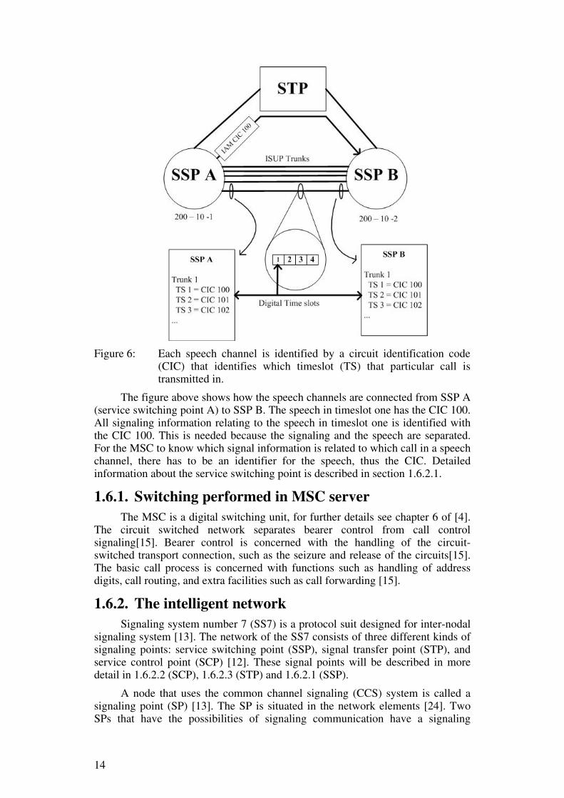
Figure 6: Each speech channel is identified by a circuit identification code
(CIC) that identifies which timeslot (TS) that particular call is transmitted in.
The figure above shows how the speech channels are connected from SSP A (service switching point A) to SSP B. The speech in timeslot one has the CIC 100. All signaling information relating to the speech in timeslot one is identified with the CIC 100. This is needed because the signaling and the speech are separated. For the MSC to know which signal information is related to which call in a speech channel, there has to be an identifier for the speech, thus the CIC. Detailed information about the service switching point is described in section 1.6.2.1.
1.6.1. Switching performed in MSC server The MSC is a digital switching unit, for further details see chapter 6 of [4].
The circuit switched network separates bearer control from call control signaling[15]. Bearer control is concerned with the handling of the circuit-switched transport connection, such as the seizure and release of the circuits[15]. The basic call process is concerned with functions such as handling of address digits, call routing, and extra facilities such as call forwarding [15].
1.6.2. The intelligent network Signaling system number 7 (SS7) is a protocol suit designed for inter-nodal
signaling system [13]. The network of the SS7 consists of three different kinds of signaling points: service switching point (SSP), signal transfer point (STP), and service control point (SCP) [12]. These signal points will be described in more detail in 1.6.2.2 (SCP), 1.6.2.3 (STP) and 1.6.2.1 (SSP).
A node that uses the common channel signaling (CCS) system is called a signaling point (SP) [13]. The SP is situated in the network elements [24]. Two SPs that have the possibilities of signaling communication have a signaling

15
relation [13]. The signaling links connecting the SS7 networks can be supported using TDM or ATM links [12].
The design of the SS7 stack is as follow. MTP layers one to three corresponds to the physical layer, the data link layer and network layer. SCCP corresponds to transport layer and supports TCAP [12].
The mode of operation can be associated, non-associated, or quasi-associated [13].
The message and its signaling relation are transmitted using the same SPs (the same route) in the associated mode of operation. Figure 7 depicts the associated mode.
Figure 7: The associated mode of operation.
In the non-associated mode of signaling, the messages belonging to a particular signaling relation are not transferred over the transmission links directly connected to the relevant SPs (as it is done in the associated mode of signaling). The messages are instead transferred using intermediate (or tandem) SPs.
The signaling network in the quasi-associated mode of operation is predetermined by information assigned by the network [13]. Figure 8 shows the quasi-associated mode of operation. Speech traffic is transferred between node X and node Y; whereas the signaling goes via node Z. Node Z is called a signal transfer point (STP) [13] .
Figure 8: The quasi-associated mode of operation.
The STP transfers signaling messages between SSP and SCP (signal control point) [3]. Details of the SSP and SCP are given below.
1.6.2.1. Service Switching Point (SSP)
The MSC is a SSP [12]. There are two main functions in a SSP: setting up and tearing down voice trunks via ISUP messages and sending SS7 messages to databases via TCAP messages [12]. The SSP connects a mobile network to an
16
intelligent network (IN). It performs the service switching function (SSF) and the call control function (CCF) [3].
When a call is made it is held at the SSP and the normal call control sequence is temporarily interrupted. This is done so an interrogation can be done to the remote IN service control point (SCP) [4]. SSPs transmit messages to the SCPs to get routing instructions or service information [12].
1.6.2.2. Service control point (SCP)
The Service Control Point (SCP) is the entity that provides the interface to database applications or service control logic [12]. It is a physical network node containing the hardware on which the control functions run [15] and is the core entity of an IN [3].
1.6.2.3. Signal transfer point (STP)
The signal transfer point’s (STP) main function is to switch and address SS7 messages. It is a kind of a message router that enables SS7 nodes to communicate with each other [12]. It routes messages using the message transfer part (MTP) [12].
1.6.2.4. Service control function (SCF)
SCF stands for service control function and is the IN function providing the remote service logic. It can be located in a separate SCP or in the SSP itself [15]. The main purpose of the SCF is to provide a software environment for the execution of the service logic programs and at the same time support functions such as signaling access and transaction control, logic program selection, provisioning, and management [15]. The SCF is able to control interaction between multiple service location protocols (SLPs) and SLP instances that invocate simultaneous [15].
The service control is provided by a multi-processor system. SS7 systems were first used in signaling for the fixed-network exchanges [4]. SS7 subsequently introduced MAP for signaling in mobile networks [4].
1.7. How calls are switched Depending on whether the mobile originates the call or receives the call, the
type of call is differentiated into two types: mobile originated call (MOC) and mobile terminated call (MTC). These two kinds of calls are handled differently in the MGW [16].
In the case of a MOC, the MGW first performs a security check to see if it should allow this call‡. If the call is allowed, the bearer set-up is established on the user plane of the caller’s side. Then a check of the subscription information is done and if the subscription permits then the call is routed to the destination address by the MSC server [16].
In the case of a MTC and if the caller is from a PSTN or another mobile network, then the call comes via a GMSC [26]. The GMSC sends the MSISDN number of the callee to the HLR to determine which HLR is responsible for the MS with this dialed number [26]. After learning the relevant HLR, the GMSC
‡ This check is not made in case of emergency calls, as all emergency calls must be allowed.
17
sends the MSISDN number to that HLR. The HLR responds with the MSRN of the MS to the GMSC. The GMSC, now knows where the MS is, hence it can route the call to the appropriate MSC [26]. This MSC queries its VLR for the TMSI corresponded to the MS with this particular MSRN number [26]. A paging message for this MS is broadcasted to all base stations belonging to this MSC [26]. A BSC managing this MS responds, now the call setup can proceed [26]. The user that receives the call is referred to as a callee [16].
The bearer service involves layers one to three in the OSI reference model. A bearer service also can be used to provide the MS with data service [16].
1.8. Protocols used in the network 1.8.1. ATM (Asynchronous mode)
The ATM is a packet switched protocol stack that uses the virtual circuit approach [10]. It is a connection oriented time division multiplexing (TDM) based on packet switching [3]. ATM can be used in high speed network backbones, such as the core and Radio Access Network (RAN). It contains three layers: the physical layer, the ATM layer and the ATM adaption layer (AAL) [10]. ATM can be used to support different kinds of subscriber services, such as voice, data and video [3]. The MSOFTX3000 support ATM signaling [3].
ATM and IP differ in several respects. ATM is connection oriented (i.e., an end-to-end connection must be established before any data can be sent), whereas IP is not. The resources along the ATM connection’s path are reserved for a specific connection, thus the path in ATM is determined during connection setup, whereas in IP each packet is independently routed[11]. Thus in ATM is a virtual connection established only after an end-to-end connection has been created [3].
There exist two types of ATM virtual service connections: the permanent virtual circuits (PVC), and the switched virtual circuits (SVC). With PVC there is direct connectivity between sites. PVC guaranties the availability of a connection and does not need call setup procedures between switches. A SVC on the other hand is created and released dynamically. The connection is maintained only as long as data is being transmitted. This is similar to a telephone call [34].
There are two types of ATM connections: the virtual path and the virtual channels. A virtual path is a set of virtual channels and is identified by a virtual path identifier (VPI). The virtual channel is identified by using the VPI it belongs to and the virtual channel identifier (VCI) [34].
The ATM reference model is composed of the physical layer, the ATM layer, the ATM adaptation layer (AAL), and the higher layers. The physical layer manages the medium-dependent transmission. The ATM layer is responsible for the simultaneous sharing of virtual circuits over a physical link. The ATM adaptation layer is responsible for hiding the details of the lower layers from the higher layer. The higher layer arranges the user data from the AAL into packets. The ATM layer two (AAL2) includes services such as packetized voice or video that do not have a constant data transmission rate [34].
ATM call control signaling uses signaling ATM adaptation layer (SAAL). SAAL is used for signaling in user-network interfaces (UNI), network-node interfaces (NNI), and in access network connecting with the host service nodes
18
[35]. The MSC uses SAAL to adapt the MT3B user layer signaling so it can be transmitted over the ATM packet network [3].
1.8.2. SS7 (Signaling system 7) SS7 is a control plane protocol stack that handles signaling messages in
fixed line telephone networks [10]. It is a packet protocol, but the transport and network layers of the SS7 (the message part) were designed for the TDM links [31]. SS7 is an out-of-band signaling protocol and offers services to both wireless and landline networks [12]. Originally SS7 used a four layer structure with the intelligent network application part (INAP) and the mobile application part (MAP) [13].
Layers one to three constitute of message transfer part (MTP). This MTP is responsible for transferring information in a message from one signaling point (SP) to another [13]. Thus the MTP transports messages and the Signaling Connection Control Part (SCCP) improves the routing capabilities of the MTP [10]. The first layer of MTP defines the physical transmission path for signaling [13] . The second layer of MTP deals with the link between two nodes. Together the layers one and two provide a reliable signaling link for transferring signaling messages [13]. The signaling information transferred between signaling points is divided into messages called signal units [13]. The layers are shown in Figure 9.
These protocol stacks can be combined. For example, ATM can be used for layer two transport in an IP network, and SS7 messages can also be transported using IP, ATM, or IP over ATM [10].
Layer four contains the user parts [13]. This layer specifies a number of call-control functions [13]. The user part is concerned with rules for connection oriented services, such as call set-up and disconnect. The controlling part is concerned with connectionless services, such as database access [12].
The SS7 also wraps up digital subscriber signaling system no. 1 (DSS1) signaling. DSS1 is used when a user requires creation of a circuit (dialing) or other services [33]. It is an access signaling system for digital lines [13] and is specified by the ITU recommendations Q.931 and Q.932 [33].
There are two main protocols in SS7: ISDN User Part (ISUP) and Bearer Connection Control Part (BCCP). ISUP is concerned with call control, while BCCP is concerned with connection control [13]. Call control is only concerned with the call and thus is independent of the traffic circuit that is used [13]. Bearer control takes care of the functions for controlling the connection [13].

19
Figure 9: Speech and control signaling flows between two nodes in a SS7
system
1.8.2.1. ISUP
ISDN User Part (ISUP) is the main application layer protocol in SS7. This protocol contains all the signaling messages that are required by the digital telephone network, such as messages for setting up a call, modifying it, and tearing it down. Earlier networks with analog transportation cannot support ISUP, instead they use the Telephone User Part (TUP) protocol. The Transaction Capabilities Application Part (TCAP) protocol works as an interface to other application layers (for those devices that do not use ISUP or TUP) [13].
1.8.2.2. BICC
The Nc-interface do not use ISUP, instead it uses bearer independent call control (BICC). BICC is an enhanced call control protocol that supports call bearer separation. The bearer used can be TDM, ATM, or IP transport [8], thus it is responsible for the bearer control of a connection [15].
1.8.2.3. MAP
The mobile application part (MAP) protocol is used for transferring mobile subscriber information from one cellular network to another. It provides rules to support mobility management, such as roaming and intersystem handover. MAP works with TCAP (Transaction Capabilities Application Part) [12] . It defines information such as message process, operation definition, data types, fault types, and specific codes [3]. It is used for communication with MSC, VLR, HLR, EIR, SMC, and GMLC (gateway mobile location centre) [3].
1.8.2.4. SCCP
The Signaling connection control part (SCCP) protocol is mainly concerned with additional routing and routing capabilities [12]. It provides global title translation (GTT). GTT is a method of summarizing routing across the network. It allows the signaling nodes of the network only to know a portion of the network [8].

20
SCCP is used especially in connection-less communication, such as used for database queries and responses [12]. SCCP is located in layer four between the MTP layers and the application layer of SS7 [8]. SCCP helps SS7 set up connectionless and connection oriented services between the MSC and other network entities such as BSC, RNC, HLR, SGSN, and GMLC [3]. SCCP also provides sub-system numbers (SSN) that identify SCCP subscribers within a single signaling point (SP) [3].
A path between the SPs is defined by a pair of source and destination IP addresses. This path is the route along which the SCTP-packets flow from one SCTP endpoint to a specific destination transport address of the endpoint’s peer SCTP endpoint [13]. SCTP is described in section 1.8.3.1.
1.8.3. SIGTRAN Signaling transport (SIGTRAN) is a standard for transporting signaling,
such as SS7, over an IP network. The signaling gateway (SG) provides an interface between the SS7 network and the SIGTRAN network. This allows transportation of SS7 traffic over IP networks [8]. The SIGTRAN architectural model is built on three components: an IP transport layer, a signaling transport protocol, and an adaption protocol. SIGTRAN uses the stream control transmission protocol (SCTP) as the signaling transport protocol [8].
SCTP is described in Section 1.8.3.1 and the signaling adaptation protocols are described in section 1.8.3.2.
1.8.3.1. SCTP
Stream control transmission protocol (SCTP) was designed as the transport layer of SIGTRAN protocol suit [3]. SCTP is a connection oriented protocol and ensures that the signaling in the IP network is efficient and reliable [13]. It enables a message based connection and supports reliable transmission of multiple media streams and provides with multiple data streams between two endpoints [14].
SCTP has been specified with a number of user adaption layers to be able to provide interworking capabilities with the SS7 network (PSTN) and IP. These user adaption layers are: SCCP user adaptation layer (SUA), MTP3 user adaptation layer (M3UA) and MTP2 user adaptation layer (M2UA) [30]. A SCTP association in MSOFT can be an M2UA link, an M3UA link, an IUA link, a H.248 link, or a BICC link [3].
1.8.3.2. Signaling adaption protocol
The M3UA uses SCTP as transport protocol for transporting signaling messages from MTP3 users (e.g. ISUP and SCCP) over the IP network. The M3UA connects the SS7 network and the IP network together. It can transport a signaling message from a signaling gateway in the SS7 network to a gateway in the IP network [30].
The M2UA supports the transportation of MTP2-user signaling (e.g. ISUP call setup messages) over IP using the SCTP. The messages being transported are MTP3 messages. This signal transport is used between a signaling gateway (SG) and a media gateway controller (MGC) or a database in IP network [27]. Figure 10 shows how the M2UA layer uses SCTP to route MTP3 messages over IP.
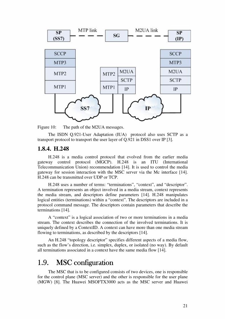
21
Figure 10: The path of the M2UA messages.
The ISDN Q.921-User Adaptation (IUA) protocol also uses SCTP as a transport protocol to transport the user layer of Q.921 in DSS1 over IP [3].
1.8.4. H.248 H.248 is a media control protocol that evolved from the earlier media
gateway control protocol (MGCP). H.248 is an ITU (International Telecommunication Union) recommendation [14]. It is used to control the media gateway for session interaction with the MSC server via the Mc interface [14]. H.248 can be transmitted over UDP or TCP.
H.248 uses a number of terms: “terminations”, “context”, and “descriptor”. A termination represents an object involved in a media stream, context represents the media stream, and descriptors define parameters [14]. H.248 manipulates logical entities (terminations) within a “context”. The descriptors are included in a protocol command message. The descriptors contain parameters that describe the terminations [14].
A “context” is a logical association of two or more terminations in a media stream. The context describes the connection of the involved terminations. It is uniquely defined by a ContextID. A context can have more than one media stream flowing to terminations, as described by the descriptors [14].
An H.248 “topology descriptor” specifies different aspects of a media flow, such as the flow’s direction, i.e. simplex, duplex, or isolated (no way). By default all terminations associated in a context have the same media flow [14].
1.9. MSC configuration The MSC that is to be configured consists of two devices, one is responsible
for the control plane (MSC server) and the other is responsible for the user plane (MGW) [8]. The Huawei MSOFTX3000 acts as the MSC server and Huawei

22
UMG8900 acts as the MGW. In the rest of the report MSOFTX3000 will be denoted MSOFT and UMG8900 will be denoted UMG to facilitate reading.
1.9.1. MSOFT The MSOFT has many interfaces for communicating with other entities in
the network. Appendix A lists the most important MSOFT interfaces and briefly describes them. Figure 11 shows the most relevant interfaces of the MSOFT.
Figure 11: Some of the interfaces of the MSC server (MSOFTX3000)
The VLR is internal to the MSOFT. The interface connecting the MSOFT with its VLR is internal. All other interfaces are external.
MSOFT supports 2G/3G convergence, as it supports GSM, 3GPP R99, 3GPP R4, and 3GPP R5 [3], by its connections to the BSS (through the A-interface) and UTRAN (through the Iu-interface) [3]. Figure 12 shows these connections, along with the relation between an MSC and the gateway MSC (GMSC). The gateway MSC connects the mobile network (in our case – Babilon M) to the PSTN or other PLMN.

23
Figure 12: MSC is composed of MSOFTX3000 and UMG8900. The A-
interface connects the MSC to the base stations (GERAN) and Iu-interface connects the MSC with the node Bs (UTRAN).
Proposed in 3GPP release 4, is the MSC is divided into a control plane element and a user plane element. The MSC server (MSOFT) is responsible for the control plane where it handles functions such as call control and signaling [8].The MGW (UMG) is responsible for the user plane where the traffic is switched [8]. The MSOFTX can act as the following network entities: VMSC server/VLR, GMSC server, TMSC server, MSC/SSP, and PVS[3].
The MSOFT supports the protocols and functions of both GSM and the WCDMA. It handles functions such as basics services (voice, SMS, GSM fax, GSM bearer, and UMTS bearer), supplementary services (defined by 3GPP), operator barring services, intelligent network (IN) services, and value-added service [3]. It also supports incoming and outgoing call connection functions of both the common and IN services [3].
The call connection functions that can be handled by the MSOFT are: local call, outgoing call, incoming call, and the incoming tandem office call [3].
1.9.2. MSOFT hardware When MSOFT uses the Huawei 750B board in full configuration it can
support 5.4 million subscribers acting as a VMSC [3].
The hardware platform in MSOFT is an open standards telecom architecture (OSTA) 1.0 platform. There can be up to 18 subracks of hardware. A standard subrack has both front board and back boards. There are two kinds of subracks: a basic subrack and expansion subracks. There has to be at least one basic subrack in a MSOFT configuration [3].
The basic subrack is the controlling subrack. It is located in frame number 0. The expansion subrack is optional. The number of expansion subracks depends on how many subscriber the MSC server will support.§ These two kinds of subracks are composed of various kinds of boards. Each type of board is responsible for a
§ The MSOFT of Kulyab has seven subracks: a basic subrack and six expansion subracks.
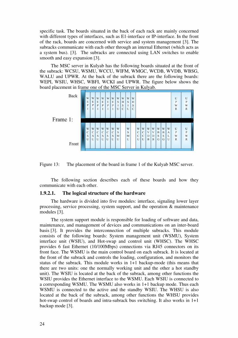
24
specific task. The boards situated in the back of each rack are mainly concerned with different types of interfaces, such as E1-interface or IP-interface. In the front of the rack, boards are concerned with service and system management [3]. The subracks communicate with each other through an internal Ethernet (which acts as a system bus). [3]. The subracks are connected using LAN switches to enable smooth and easy expansion [3].
The MSC server in Kulyab has the following boards situated at the front of the subrack: WCSU, WSMU, WCCU, WIFM, WMGC, WCDB, WVDB, WBSG, WALU and UPWR. At the back of the subrack there are the following boards: WEPI, WSIU, WHSC, WBFI, WCKI and UPWR. The figure below shows the board placement in frame one of the MSC Server in Kulyab.
Figure 13: The placement of the board in frame 1 of the Kulyab MSC server.
The following section describes each of these boards and how they communicate with each other.
1.9.2.1. The logical structure of the hardware
The hardware is divided into five modules: interface, signaling lower layer processing, service processing, system support, and the operation & maintenance modules [3].
The system support module is responsible for loading of software and data, maintenance, and management of devices and communications on an inter-board basis [3]. It provides the interconnection of multiple subracks. This module consists of the following boards: System management unit (WSMU), System interface unit (WSIU), and Hot-swap and control unit (WHSC). The WHSC provides 6 fast Ethernet (10/100Mbps) connections via RJ45 connectors on its front face. The WSMU is the main control board on each subrack. It is located at the front of the subrack and controls the loading, configuration, and monitors the status of the subrack. This module works in 1+1 backup-mode (this means that there are two units: one the normally working unit and the other a hot standby unit). The WSIU is located at the back of the subrack, among other functions the WSIU provides the Ethernet interface to the WSMU. Each WSIU is connected to a corresponding WSMU. The WSMU also works in 1+1 backup mode. Thus each WSMU is connected to the active and the standby WSIU. The WHSU is also located at the back of the subrack, among other functions the WHSU provides hot-swap control of boards and intra-subrack bus switching. It also works in 1+1 backup mode [3].
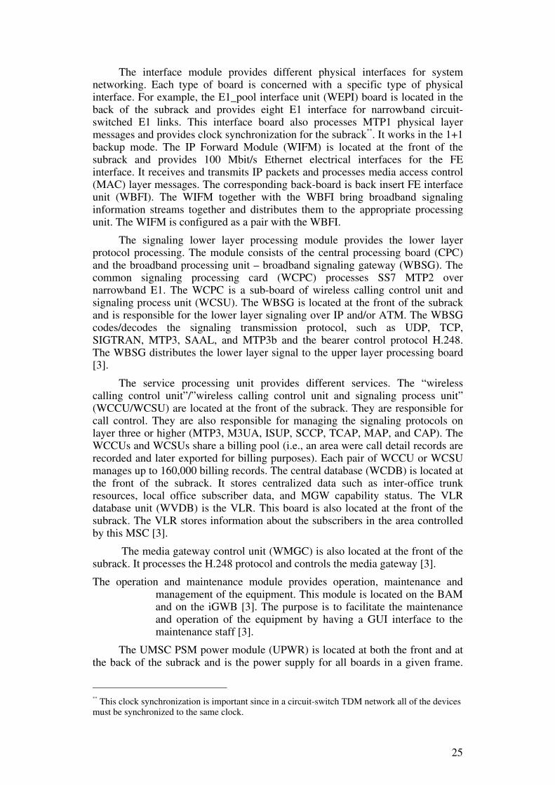
25
The interface module provides different physical interfaces for system networking. Each type of board is concerned with a specific type of physical interface. For example, the E1_pool interface unit (WEPI) board is located in the back of the subrack and provides eight E1 interface for narrowband circuit-switched E1 links. This interface board also processes MTP1 physical layer messages and provides clock synchronization for the subrack**. It works in the 1+1 backup mode. The IP Forward Module (WIFM) is located at the front of the subrack and provides 100 Mbit/s Ethernet electrical interfaces for the FE interface. It receives and transmits IP packets and processes media access control (MAC) layer messages. The corresponding back-board is back insert FE interface unit (WBFI). The WIFM together with the WBFI bring broadband signaling information streams together and distributes them to the appropriate processing unit. The WIFM is configured as a pair with the WBFI.
The signaling lower layer processing module provides the lower layer protocol processing. The module consists of the central processing board (CPC) and the broadband processing unit – broadband signaling gateway (WBSG). The common signaling processing card (WCPC) processes SS7 MTP2 over narrowband E1. The WCPC is a sub-board of wireless calling control unit and signaling process unit (WCSU). The WBSG is located at the front of the subrack and is responsible for the lower layer signaling over IP and/or ATM. The WBSG codes/decodes the signaling transmission protocol, such as UDP, TCP, SIGTRAN, MTP3, SAAL, and MTP3b and the bearer control protocol H.248. The WBSG distributes the lower layer signal to the upper layer processing board [3].
The service processing unit provides different services. The “wireless calling control unit”/”wireless calling control unit and signaling process unit” (WCCU/WCSU) are located at the front of the subrack. They are responsible for call control. They are also responsible for managing the signaling protocols on layer three or higher (MTP3, M3UA, ISUP, SCCP, TCAP, MAP, and CAP). The WCCUs and WCSUs share a billing pool (i.e., an area were call detail records are recorded and later exported for billing purposes). Each pair of WCCU or WCSU manages up to 160,000 billing records. The central database (WCDB) is located at the front of the subrack. It stores centralized data such as inter-office trunk resources, local office subscriber data, and MGW capability status. The VLR database unit (WVDB) is the VLR. This board is also located at the front of the subrack. The VLR stores information about the subscribers in the area controlled by this MSC [3].
The media gateway control unit (WMGC) is also located at the front of the subrack. It processes the H.248 protocol and controls the media gateway [3].
The operation and maintenance module provides operation, maintenance and management of the equipment. This module is located on the BAM and on the iGWB [3]. The purpose is to facilitate the maintenance and operation of the equipment by having a GUI interface to the maintenance staff [3].
The UMSC PSM power module (UPWR) is located at both the front and at the back of the subrack and is the power supply for all boards in a given frame.
** This clock synchronization is important since in a circuit-switch TDM network all of the devices must be synchronized to the same clock.
26
The clock interface unit (WCKI) is located at the back of the subrack and is responsible for system synchronization. The alarm unit (WALU) is located at the front of the subrack and is responsible for alarm functions. The LAN bus carriers the signaling traffic streams between service subracks [3].
1.9.2.2. The hardware configuration of the MSC server of Kulyab
Table 1 and Table 2 show the hardware configuration (in terms of the numbers of each type of board) of the MSC server of Kulyab. The basic subrack contains frame number 0. As shown in these two tables, the boards that only are located in frame zero are: (in the front) WIFM, WMGC, WCDB and (in the back) WBFI and WCKI. The WCDB is the central database unit of the MSC server, and the WMGC is the media gate controller unit. WIFM and WBFI are configured and works together as a paired unit. The VLR boards (the WVDB) are all located in frame one.
Table 1: The placement of the front boards in the MSC server in Kulyab. “H” stands for “having” that type of board. The symbol, “-“, stands for not having that type of board.
Frame Number 0 1 2 3 4 5 6 7WCSU H H - - H - - HWSMU H H H H H H H HWCCU H H H H H H H HWIFM H - - - - - - -WMGC H - - - - - - -WCDB H - - - - - - -WVDB - H - - - - - -WBSG - H H H H H H HWALU H H H H H H H HUPWR H H H H H H H H
Table 2: Shows the placement of the back boards in the MSC server in Kulyab.
Frame Number 0 1 2 3 4 5 6 7WEPI H H - - H - - HWSIU H H H H H H H HWHSC H H H H H H H HWBFI H - - - - - - -WCKI H - - - - - - -UPWR H H H H H H H H
The boards working in 1+1 backup mode are: (at the front) WCSU, WSMU, WCCU, WIFM, WMGC, WCDB WVDB, and (at the back) WEPI, WSIU, WHSC, WBFI. When boards work in the 1+1 backup mode they work in pairs. One is active and the other one is a hot standby. The standby board is periodically updated with the data from the active board, so that if necessary it can take over quickly. WBSG, situated at the front, works in load sharing mode. In load sharing mode, the same type of boards within a functional subrack share the tasks between themselves.

27
1.9.3. Software structure The MSOFT software can be divided into host software and background
software [3].
1.9.3.1. The host software
The host software together with the background software can perform: data management; equipment management; alarm management; and perform measurement, signaling trace, and CDR management [3]. Software and configurations are loaded via the “shared resource bus” in each frame. This bus is managed by the WSMU [48].
The host software has a layered modular design and consists of: a real time operating system, middleware, and application software[3]. The application software is divided into five different parts: the signaling bearer software, the service processing software, the database software, the system support software, and the operations and maintenance (O&M software) [3]. The boards belong to each of these parts of the application software are shown in Table 3.
Table 3: Boards and their corresponding application software
Boards Application softwareWBSG signaling bearer WBFI signaling bearer WEPI signaling bearer WIFM signaling bearer
WCSU service processing WCCU service processing WMGC service processing
WCDB database WVDB database
WSMU system support WHSC system support
WSMU +all boards O&M
The signaling bearer software accesses both broadband and narrowband signaling links. The boards configured with the signaling bearer software are responsible for processing lower layer protocols. The boards configured with the service processing software are responsible for signaling processing, call processing, mobility management, and resource management. The boards configured with the database software are responsible for database management. The boards configured with the system support software perform system management and device interworking. The O&M software is configured in all boards, but mainly in WSMU. It provides the interface between the Back administration module (BAM) and the boards [3].
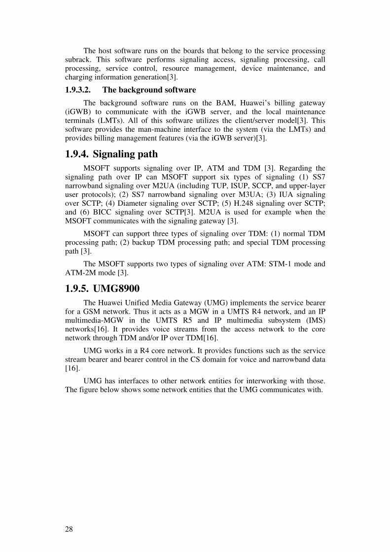
28
The host software runs on the boards that belong to the service processing subrack. This software performs signaling access, signaling processing, call processing, service control, resource management, device maintenance, and charging information generation[3].
1.9.3.2. The background software
The background software runs on the BAM, Huawei’s billing gateway (iGWB) to communicate with the iGWB server, and the local maintenance terminals (LMTs). All of this software utilizes the client/server model[3]. This software provides the man-machine interface to the system (via the LMTs) and provides billing management features (via the iGWB server)[3].
1.9.4. Signaling path MSOFT supports signaling over IP, ATM and TDM [3]. Regarding the
signaling path over IP can MSOFT support six types of signaling (1) SS7 narrowband signaling over M2UA (including TUP, ISUP, SCCP, and upper-layer user protocols); (2) SS7 narrowband signaling over M3UA; (3) IUA signaling over SCTP; (4) Diameter signaling over SCTP; (5) H.248 signaling over SCTP; and (6) BICC signaling over SCTP[3]. M2UA is used for example when the MSOFT communicates with the signaling gateway [3].
MSOFT can support three types of signaling over TDM: (1) normal TDM processing path; (2) backup TDM processing path; and special TDM processing path [3].
The MSOFT supports two types of signaling over ATM: STM-1 mode and ATM-2M mode [3].
1.9.5. UMG8900 The Huawei Unified Media Gateway (UMG) implements the service bearer
for a GSM network. Thus it acts as a MGW in a UMTS R4 network, and an IP multimedia-MGW in the UMTS R5 and IP multimedia subsystem (IMS) networks[16]. It provides voice streams from the access network to the core network through TDM and/or IP over TDM[16].
UMG works in a R4 core network. It provides functions such as the service stream bearer and bearer control in the CS domain for voice and narrowband data [16].
UMG has interfaces to other network entities for interworking with those. The figure below shows some network entities that the UMG communicates with.

29
Figure 14: The UMG communicates with the NEs through interfaces.
The UMG communicates with the radio network controller (RNC) through the Iu-interface, with the MGC (media gateway controller) through the Mn-interface and with the adjacent MGWs through the Nb-interface [16]. The MGC controls the MGW by using the H.248 protocol. The transmission channel for bearer setup is done through the Nb-interface. To complete call routing and control services are the MGCs connected to each other through Nc-interface [16].
The UMG have two types of Iu-interface: an ATM interface and an IP interface [16].
1.9.5.1. Service switching module hardware platform
The service switching module (SSM) is the core unit of a UMG and it provides an interface to the MSOFT. It implements switching, processing, and forwarding of service streams and also exchanges gateway control messages [16]. The UMG uses SSM-256 frames [16]. Each SSM-x frame can handle x TDM calls, where x is 4K, 16K, or 256K. An SSM-256 has an aggregate throughput of 128 Gbps (Chapter 3, page 110 of [49]).
1.9.5.2. The hardware structure of the UMG
The hardware structure of the UMG consists of four different kinds of frames: the central switch frame (frame zero), the main control frame (frame one), the control frame (always frame eight), and the service frames (in our case frames two to five). It is only when there are six service frames (frame two to seven) that a control frame is needed. This is because having a large number of service frames requires extra control capacity.
The main control frame (frame one) is the control and management center of the entire UMG. It also provides the clock signal to the other frames. The central switching frame (frame zero) provides the UMG with switching and cascading

30
functions between frames and service processing functions. The control frame (last frame) processes control messages. However, this description only applies to large-scale SSM-256 frames where there are seven service frames (there is no control frame for the MGW in Kulyab because there are only four service frames). The service frames are responsible for processing service functions and provide the interface to the UMG [16].
TDM, fast Ethernet (FE), and gigabit Ethernet (GE) cascading are available between frames. The cascading channels operate in master-slave mode.
1.9.5.3. The logical structure of the hardware
The UMG is composed of cabinets that contain different kinds of boards that are responsible for a certain task or function, similar to structure of the MSOFT. Each board has a logical board name and a physical board name. The logical board name is used for configuration and would be listed in alarm output, while the physical board name identifies the actual board. Each logical board can include one or more physical boards. A physical board belonging to a given logical board name can have a different interface, performance, and be located in a specific frame and board slot [16].
The management and control module is responsible for management and maintenance. It is connected via the BAM to the LMT. This module is also controls the gateway controller to invoke bearer and service resources, setting up service bearers, and processing service stream formats [16]. This module includes the operations and management unit (OMU), main processing unit (MPU), Protocol processing unit (PPU), and Connection & management unit (CMU).
The packet processing module consists of two parts: packet switching and the packet processing & interface. The hardware for packet processing and interface is divided into those elements which handle IP packets and those which handle ATM cells. The NET-board provides packet switching. Table 4 shows the different types of boards and what module they belong to [16].
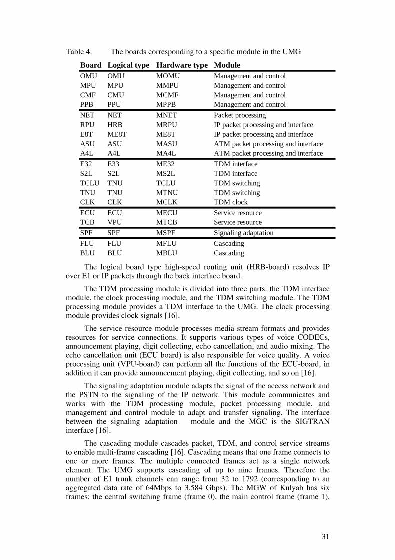
31
Table 4: The boards corresponding to a specific module in the UMG
Board Logical type Hardware type Module OMU OMU MOMU Management and controlMPU MPU MMPU Management and controlCMF CMU MCMF Management and controlPPB PPU MPPB Management and controlNET NET MNET Packet processing RPU HRB MRPU IP packet processing and interfaceE8T ME8T ME8T IP packet processing and interfaceASU ASU MASU ATM packet processing and interfaceA4L A4L MA4L ATM packet processing and interfaceE32 E33 ME32 TDM interfaceS2L S2L MS2L TDM interfaceTCLU TNU TCLU TDM switchingTNU TNU MTNU TDM switchingCLK CLK MCLK TDM clockECU ECU MECU Service resource TCB VPU MTCB Service resource SPF SPF MSPF Signaling adaptation FLU FLU MFLU CascadingBLU BLU MBLU Cascading
The logical board type high-speed routing unit (HRB-board) resolves IP over E1 or IP packets through the back interface board.
The TDM processing module is divided into three parts: the TDM interface module, the clock processing module, and the TDM switching module. The TDM processing module provides a TDM interface to the UMG. The clock processing module provides clock signals [16].
The service resource module processes media stream formats and provides resources for service connections. It supports various types of voice CODECs, announcement playing, digit collecting, echo cancellation, and audio mixing. The echo cancellation unit (ECU board) is also responsible for voice quality. A voice processing unit (VPU-board) can perform all the functions of the ECU-board, in addition it can provide announcement playing, digit collecting, and so on [16].
The signaling adaptation module adapts the signal of the access network and the PSTN to the signaling of the IP network. This module communicates and works with the TDM processing module, packet processing module, and management and control module to adapt and transfer signaling. The interface between the signaling adaptation module and the MGC is the SIGTRAN interface [16].
The cascading module cascades packet, TDM, and control service streams to enable multi-frame cascading [16]. Cascading means that one frame connects to one or more frames. The multiple connected frames act as a single network element. The UMG supports cascading of up to nine frames. Therefore the number of E1 trunk channels can range from 32 to 1792 (corresponding to an aggregated data rate of 64Mbps to 3.584 Gbps). The MGW of Kulyab has six frames: the central switching frame (frame 0), the main control frame (frame 1),

32
the control frame (frame 5), and service frames (frames 2 to 4). Figure 15 shows the cascading used in the MGW of Kulyab [16].
There are two types of MNETs: the UG01MNET and the UG02MNET. The MGW of Kulyab has an MNET of type UG01MNET. The capacity of a UG01MNET is 16 GE cascading (for an aggregate of 16 Gbit/s of packet switching capacity). The Fe1 interface on the MNET boards is used for FE cascading between frames [16].
Figure 15: Self-cascading in the MGW of Kulyab with six frames. Where the
dashed line GE indicates Gigabit Ethernet service data plane links and the solid line FE indicates Fast Ethernet service control planes.
1.9.5.4. The boards in the MGW in Kulyab
Table 5 and Table 6 show the hardware configuration of the MGW of Kulyab. The main control frame is frame number 1. This frame has OMU-boards located at the front of the frame. The other frames have MPU-boards at the front instead of an OMU. The CLK-board is only located in the main control frame. The central switch frame is frame number 0. It is the only frame that has the front link unit (FLU) and back link unit (BLU) boards. It also has the TDM central
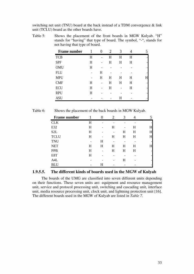
33
switching net unit (TNU) board at the back instead of a TDM convergence & link unit (TCLU) board as the other boards have.
Table 5: Shows the placement of the front boards in MGW Kulyab. “H” stands for “having” that type of board. The symbol, “-“, stands for not having that type of board.
Frame number 1 0 2 3 4 5TCB H - H H H -SPF H - H H H -OMU H - - - - -FLU - H - - - -MPU - H H H H HCMF H - H H H -ECU H - H - H -RPU H - - - - -ASU - - - H - -
Table 6: Shows the placement of the back boards in MGW Kulyab.
Frame number 1 0 2 3 4 5CLK H - - - - -E32 H - H - H HS2L H - - H H HTCLU H - H H H HTNU - H - - - -NET H H H H H HPPB H - H H H -E8T H - - - - -A4L - - - H - -BLU - H - - - -
1.9.5.5. The different kinds of boards used in the MGW of Kulyab
The boards of the UMG are classified into seven different units depending on their functions. These seven units are: equipment and resource management unit, service and protocol processing unit, switching and cascading unit, interface unit, media resource processing unit, clock unit, and lightning protection unit [16]. The different boards used in the MGW of Kulyab are listed in Table 7.

34
Table 7: Displays the unit and the corresponding boards for each board used in the MGW of Kulyab.
Logical Hardware Corresponding Board type type Unit board
OMU OMU MOMU equipment and resource management NETMPU MPU MMPU equipment and resource management NETCMF CMU MCMF equipment and resource management -PPB PPU MPPB equipment and resource management -RPU HRB MRPU service and protocol processing E8TE8T ME8T ME8T interface HRBNET NET MNET switching and cascading OMU/MPUASU ASU MASU service and protocol processing A4LA4L A4L MA4L interface ASUE32 E32 ME32 interface -S2L S2L MS2L interface -TCLU TNU TCLU switching and cascading -TNU TNU MTNU switching and cascading -CLK CLK MCLK ClockECU ECU MECU media resource processing -TCB VPU MTCB media resource processing -SPF SPF MSPF service and protocol processing -FLU FLU MFLU switching and cascading BLUBLU BLU MBLU switching and cascading FLU
The equipment and resource management unit consists of OMU, MPU, CMU, and PPU. The OMU (MOMU) manages all the frames of the MGW when using multi-frame cascading. The MGW OMU implements the switching function of the data planes for broadband services and provides external interfaces. The MGW MPU (MMPU) manages the frame where it is located. It implements the switching function of the data planes for broadband services. The MGW CMU (MCMF) processes messages from the media resource control protocol and operates the corresponding resources. The MGW PPU (MPPB) processes the H.248, SCTP, UDP, TCP, and IP protocols. It also provides an external FE interface [16].
The service and protocol processing unit consists of high-speed routing unit (HRB), ATM AAL2/AAL5 SAR processing unit (ASU) and front signaling processing unit (SPF). The MGW HRB (MRPU) processes IP routes and distributes IP services and provides access services. The MGW ASU (MASU) processes ATM services. The MGW SPF (MSPF) performs signaling adaptations and signal transferring.
The switching and cascading unit consists of packet switch unit (NET), front link unit (FLU), back link unit (BLU), and TDM central switching net unit (TNU). The MGW NET (MNET) implements the packet server switching function and the data cascading between frames. The FLU and BLU provides TDM broadband interfaces and TDM switching functions. They have 32 k cascading capacity. The BLU also provides a 100 Mbit/s control data channel to directly connect frames for cascading. The TNU has two types of hardware boards: the MGW TDM switching net unit (MTNU) and the TDM convergence &
35
link unit (TCLU). Both implement TDM service switching. They provide 3x8k TDM cascading interfaces and 24k TDM timeslot cascading function.
The interface unit consists of combination of 2*155M SDH/SONET optical interface card (S2L), 4 port STM-1 ATM optical interface board (A4L), 8-port 10/100 Ethernet interface board (E8T), or 32*E1 port TDM interface board (E32). The MGW S2L (MS2L) provides two 155 Mbit/s optical interfaces. The MGW A4L (hardware type MA4L) provides four 155 Mbit/s ATM optical interfaces. The MGW E8T (ME8T) provides with eight fast Ethernet interfaces. MGW E32 (ME32) provides 32 E1 interfaces to receive and send signaling from Channel association signaling (CAS).
The media resource processing unit consists of some combination of VPU and ECU boards. The MGW VPU (MTCB) provides announcement playing resources. The MGW ECU (MECU) implements echo cancellation function for voice signals. It works with together with voice sub boards.
The clock unit consists of the clock unit (CLK). It provides clock signals for services and provides with external interfaces.
1.10. Analyzing method for mobile traffic Depending on the porpoise of the analysis one uses different parameters to
analyze the traffic. Section 1.10.1 describes which parameters are used when analyzing the traffic to enhance it. Section 1.10.2 introduces the traffic flow and the parameters used when analyzing the traffic flow. Section 1.10.3 describes when planning a network.
1.10.1. The parameters used in analyzing quality of traffic
The parameters being analyzed depend on the purpose of the work. For coverage requirements it is the signal levels for outdoor, in-car, and indoor with different coverage probabilities. For the quality requirements it is the drop MS call rate and call blocking parameters [5].
The main quality parameters are call success rate (or dropped call rate), handover success rate, congestion or call attempt success rate, and customer observed downlink (DL) quality [5]. Typically target values for those parameters are shown in Table 8.

36
Table 8:The quality parameters with their target values
Quality parameter Target value
Drop call rate < 5 %
Handover success rate > 95 %
Call attempt success rate > 98 %
DL quality > RXQUAL 5
DL quality is measured in terms of bit error rate (BER) and mapped to received quality (RXQUAL) values as defined in GSM technical specification 05.08 section 8.2.4[22]. The mapping between BER and RXQUAL is shown in Table 9. Normally downlink RXQUAL classes 0 to 5 are considered to be sufficient call quality for the end user, while classes 6 and 7 are considered poor performance and should be avoided. The target value for RXQUAL can be, for example, 95 % of the time equal or better than 5. Example values for network quality targets are shown in Table 2.2 of [5].
Table 9: RXQUAL parameter ranges based upon BER before channel decoding, adapted from table in section 8.2.4 on page 22 of [22]
RXQUAL_0 BER < 0.2%
RXQUAL_1 0.2% < BER < 0.4%
RXQUAL_2 0.4% < BER < 0.8%
RXQUAL_3 0.8% < BER < 1.6%
RXQUAL_4 1.6% < BER < 3.2%
RXQUAL_5 3.2% < BER < 6.4%
RXQUAL_6 6.4% < BER < 12.8%
RXQUAL_7 12.8% < BER
There are other important sources of data worth examining. For example, an accurate digital map -- together with the propagation model can be used to calculate the coverage area of cells during the planning phase[15].
Population data are needed to estimate numbers of potential subscribers, as knowledge of the potential numbers of subscribers is necessary to estimate the needed capacity. The available bandwidth (as assigned to this operator) is also an important network planning parameter. Some basic decisions are dependent on the bandwidth, base station configuration, and frequency planning[5].
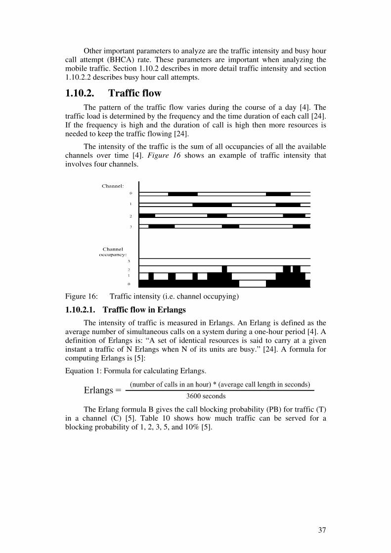
37
Other important parameters to analyze are the traffic intensity and busy hour call attempt (BHCA) rate. These parameters are important when analyzing the mobile traffic. Section 1.10.2 describes in more detail traffic intensity and section 1.10.2.2 describes busy hour call attempts.
1.10.2. Traffic flow The pattern of the traffic flow varies during the course of a day [4]. The
traffic load is determined by the frequency and the time duration of each call [24]. If the frequency is high and the duration of call is high then more resources is needed to keep the traffic flowing [24].
The intensity of the traffic is the sum of all occupancies of all the available channels over time [4]. Figure 16 shows an example of traffic intensity that involves four channels.
Figure 16: Traffic intensity (i.e. channel occupying)
1.10.2.1. Traffic flow in Erlangs
The intensity of traffic is measured in Erlangs. An Erlang is defined as the average number of simultaneous calls on a system during a one-hour period [4]. A definition of Erlangs is: “A set of identical resources is said to carry at a given instant a traffic of N Erlangs when N of its units are busy.” [24]. A formula for computing Erlangs is [5]:
Equation 1: Formula for calculating Erlangs.
The Erlang formula B gives the call blocking probability (PB) for traffic (T)
in a channel (C) [5]. Table 10 shows how much traffic can be served for a blocking probability of 1, 2, 3, 5, and 10% [5].

38
Table 10: Erlang B for blocking probabilities of 1, 2, 3, 5, and 10%, adapted from table 2.13 in section 2.6.1 of [5].
Blocking probability 1% 2% 3% 5% 10%Channels
1 0.01 0.02 0.03 0.05 0.112 0.15 0.23 0.28 0.38 0.63 0.46 0.6 0.71 0.9 1.274 0.87 1.09 1.26 1.53 2.055 1.36 1.66 1.87 2.22 2.886 1.91 2.28 2.54 2.96 3.767 2.5 2.93 3.25 3.74 4.678 3.13 3.63 3.99 4.54 5.69 3.78 4.34 4.75 5.37 6.5510 4.46 5.09 5.53 6.21 7.5115 8.11 9.01 9.65 10.63 12.4820 12.03 13.18 14 15.25 17.6125 16.12 17.5 18.48 19.98 22.8330 20.34 21.93 23.06 24.8 28.11
The table shows that with 15 channels and with a blocking probability of 2% then the 15 channels can serve 5.09 Erlangs of load. Trunking gain is calculated by using the same table, and dividing by the number of channels. The first seven channels correspond to one TRX when one time slot out of eight is reserved for signaling. Channel 30 belongs to three TRX cases, i.e. when two timeslots out of 32 are reserved for signaling.
When the blocking probability is 2% and the trunk has 7 channels then the trunking gain is 0.42 Erlangs/channel (2.93 Erlangs/7 channels). If the trunk has 30 traffic channels and uses 2 timeslot for signaling then the trunking gain will be 0.69 Erlangs/channel (21.93 Erlangs/32 channels) [5].
A traffic profile can be done using hours of a whole day along the x-axis and traffic in Erlangs or call attempts/seconds along the y-axis (CA/S) [24]. The distribution of traffic in Erlangs during a day will vary with the time of day. There will be peak hours and low intensity hours during a day [24]. Besides variations during a day, there will also be variations according to national holidays and other festivity days [24]. There are three different traffic profiles[24]:
Normal day corresponds to usual activity during a day(Load A)
High load condition corresponds to special days in a year(for instance Mothers day) (Load B)
Exceptional conditions conditions not provisioned (Overloaded)
It is important that the configuration can serve at least the mobile traffic of load A, but it is very good if it also can serve the traffic of load B [24]. It is very difficult to meet the third condition, because this load corresponds to a unpredictable situation [24].

39
For analyzing the traffic load intensity for the conditions of load A, it is necessary to analyze the traffic for at least one month [24]. A set of days are chosen and ordered from the lowest to highest daily peak traffic intensity measurements. The fourth highest value will be chosen as the normal load traffic intensity [24]. The reference load A represents the normal upper mean value that is offered to the subscribers [24].
1.10.2.2. Busy hour caller attempts (BHCA)
“Busy hour caller attempts” denotes one measure of traffic load in a network [24]. It is the number of caller attempts to initiate a call during the busiest hour, thus when there is peak traffic. A call attempt occurs when a subscriber attempts to make a call [24]. Thus the call attempt is the attempt to set up a call. There can be two outcomes: success or failure [24]. An unsuccessful call attempt can be caused by incomplete dialing, called party busy or no response, etc. [24].
The control plane is mainly concerned with BHCA, while the user plane is concerned with Erlangs [24].
1.10.3. Planning It is important to estimate the traffic flow between exchanges (MSC) in both
directions (i.e. incoming and outgoing traffic). In the absence of data, a gravitational formula can be used to estimate: traffic between A and B = (population of A) x (population of B) / distance2 [4]. However, in our case these flows will be determined from measurements of existing calling distributions as the operator already has base stations deployed in the target region. In the case of release 4, the limitation of the MSC server is concerned with BHCA and the limitation for the MGW is concerned with Erlangs [25]. The real bottleneck is the maximum BHCA [25].
Erlang reflects the switching capacity and port capacity of the MSC, whereas BHCA reflects the processing power of the MSC. Erlangs can be increased by adding extra MGW hardware, but the maximum BHCA is fixed for a given release of the MSC. Thus one can add hardware (adding Erlangs of call capacity) only up until the maximum BHCA is reached. Adding hardware after reaching this BHCA limit is useless, as it has no effect. For voice traffic the important calculation is thus BHCA-based on a given market [25].
Commercial MSC servers usually have a BHCA-limitation of 300,000 to 500,000 BHCA, but this number will surely increase in the future [25].
A characterization of the traffic in the user plane and control plane is essential before calculating the traffic load [24]. For example, what kinds of services will be provided? A voice call, for instance, is characterized by a call arrival law (usually Poison), a call duration (usually exponential with a mean value of some minutes), and a constant bit rate (64 Kbit/s) [24]. Besides the service characterization, there is also the traffic mix. What kinds of subscriber use the network? By knowing the kind of subscriber, one also knows what kind of services they usually require [24]. The distribution of traffic flows are also very important [24]. Computing a traffic matrix, one can see the distribution of traffic very well [24].
After the traffic is estimated, this load can be computed and mapped to the physical cable infrastructure, i.e. to perform traffic engineering of the routes [4].

40
1.10.3.1. Initial traffic measurements The initial traffic for the MSC-Kulyab to/from MSC-Dushanbe is estimated
to be 0.2292 (relates to the highest measured value for connect traffic in Erlangs) during the busiest hour, while the traffic between MSC-Kulyab to/from MSC-RRP is estimated to be 0.0472 (relates to the highest measured value for connect traffic in Erlangs) during the busiest hour. This traffic corresponds to a speed of 64 kbps to/from MSC-Dushanbe and of 64 kbps to/from MSC-RRP. Additional signaling traffic between MSC-Kulyab and MSC-Dushanbe is estimated to be 64 kbps and 64 kbps between MSC-Kulyab and MSC-RRP.
1.10.3.2. Cost reduction
The estimates in the previous section suggest that there will be a cost reduction of US$ 5.4 million per year versus the current cost of back-haul connections between each of the base stations and MSC-RRP.

41
2. Collection of statistic The goal of the thesis project is to analyze the Kulyab traffic load and
examine how well the traffic fits the maximum capacity of the MSC in Kulyab as configured.
Knowing the maximum capacity of the MSC in Kulyab as it is configured is essential in this process. An analysis of the traffic generated in Kulyab is also necessary. If the traffic in Kulyab region is higher than what the MSC can support, then a smaller area has to be chosen and analyzed. Statistics regarding Kulyab traffic were collected from the 23rd of February to the 25th of March.
An important and interesting question is how the efficiency of MSC-RRP will increase when the traffic of Kulyab will move to its own MSC. The capacity of the MSC-RRP will increase when the mobile traffic of the base stations in Kulyab moves to their own MSC. To be able to calculate the increase in capacity, the capacity with and without the Kulyab traffic has to be calculated. Besides of that, the maximum capacity of the MSC-RRP as it is configured has also to be calculated.
The statistics for the overall 2G traffic generated through the MSC-RRP have been collected. The measurement period was from the 16th of May to the 22nd of May. There are two measurement period because the collection of statistics from the MSC-RRP was not collected earlier. This was not planned. The statistics from MSC-RRP should have been collected at the same time as the Kulyab traffic.
The traffic has thus been collected for all traffic in MSC-RRP and Kulyab region. Then a calculation of the traffic through MSC-RRP without the Kulyab traffic can be computed. The percentage of Kulyab traffic has been calculated. The maximum capacity has also been calculated for the MSC-RRP as it is configured.
The increased capacity will be calculated from the formula:
Equation 2: Calculation of the increased capacity for the MSC-RRP
The increased capacity will be expressed in terms of both Call attempts
(BHCA) and in Erlangs (connect traffic).
All values in the thesis project will use relative values. The highest measured value (HMV) measured in the analyzed period will be used as the value against which the other values will be compared to.

42
2.1. Calculation of the maximum capacity of the MSC as configured
The maximum capacity will be calculated for the MSC in Kulyab as configured and for the MSC-RRP as configured. The calculation of the capacity for the MSC requires knowing which kinds of boards manage the capacity and how many there are. This information can be collected directly from the BAM. From the specifications of the boards in the Huawei manual concerning MSOFT (MSC server) [3] and UMG (MGW) [16] one can find out which boards handle the capacity. Knowing the capacity boards and how many they are, one can calculate the maximum capacity of the MSC. The key limitation for the MSC server is the maximum busy hour call attempts (BHCA) and for the MGW the maximum traffic flow in Erlangs. As a result, the traffic load will be analyzed in terms of both BHCA and Erlangs. The specific configuration of the MSC server determines the maximum BHCA it supports, while the specific configuration of the MGW determines the maximum traffic in Erlangs it can support.
The capacity of the MSC in Kulyab will determine if it can support the traffic generated in this area or not. The capacity of the MSC and the traffic load will be expressed in relative numbers. The BHCA value will be related to the highest measured value of BHCA (BHMV) measured during the period for the traffic in Kulyab. The traffic load value will relate to the highest value measured regarding connect traffic (CHMV) in the measurement period for Kulyab region.
The calculation of the maximum capacity of the MSC-RRP is calculated in the same way as for the MSC in Kulyab. The boards that determine the capacity are calculated in the MSC server and in the MGW.
The maximum capacity of the MSC-RRP as configured will be used to calculate its capacity gain in terms of BHCA and the connected traffic load.
The maximum capacity of the MSCs depends how they are configured. Section 3.1.1 on page 53 describes how the maximum capacity for the MSC server in Kulyab as configured is calculated. Section 3.1.2 on page 56 describes how the maximum capacity for the MGW in Kulyab as configured is calculated. The capacity for the MSC server in RRP as configured is calculated in section 3.3.1.1 on page 98 and for the MGW-RRP in section 3.3.1.2 on page 98.

43
2.2. Calculation of the traffic statistics The interesting parameters are the BHCA (Busy hour call attempt) load and
the load of the traffic flow (the connected traffic load and responded traffic load) in Erlangs. BHCA value defines the traffic load in the control plane and the load for connected traffic and responded traffic define the traffic load in the user plane. They express the traffic capacity generated by the subscribers [24].
The BHCA denotes the control signaling load in the control plane and its unit is “number of call attempts” [24]. The BHCA is measured for each hour. It denotes how many call attempts there are made in an hour [3]. This parameter measures the signaling traffic load [24].
There are two parameters of the traffic flow to measure: the connected traffic load and the responded traffic load. The connected traffic load is measured from the successful bearer setup until it is released (i.e. from the time when the bearer setup is established between caller and callee until the call is released). The call does not need to be picked up [3]. The responded traffic load is measured from when the call is responded until it is released. Both the connected traffic load and responded traffic load have the unit Erlangs [3]. Because the connected traffic load is measured from when the call is successfully connected (i.e. a measure point before the responded traffic load) to its release, the connected traffic load is thus always higher than the responded traffic load.
The response times are also described in the thesis. The response times is measured when the call is responded and its unit is “call attempts”, thus the same as for BHCA value [3]. This parameter is used when calculating the average duration of a call. The average call duration is calculated by multiplying the responded traffic with 3600 and divided it by number of calls. The unit of the average call duration is in seconds.
Each parameter in the statistics was collected with regard to MOC and MTC. In the thesis, the MOC and MTC are added together for each parameter (i.e. the BHCA for example has a MOC and MTC part). The values throughout the thesis use relative values to protect details of the real values of the traffic. The section 2.2.1 describes in more detail the relative values.
2.2.1. Relative values The values are relative to the highest measured value (HMV) for the
analyzed period (23rd of February to the 25th of March 2011). The HMV for BHCA (BHMV) is used for those parameters regarding BHCA or parameters with the unit “number of call attempts”. The HMV for connected traffic (CHMV) is used for parameters regarding traffic flow with the unit “Erlangs”.
When comparing the Kulyab traffic with the overall traffic in MSC-RRP, a relative percentage will be used (rel. %). A relative percentage will be used for BHCA traffic and another for the connect traffic flow in Erlangs. These two values have been chosen to be the maximum percentage of Kulyab traffic measured in the period 16th of May to 22nd of May 2011.
All values throughout the thesis will relate to one of these relative values. There are two measurement periods because the collection of statistics
regarding the calculation of the capacity gain for the MSC-RRP was not collected at the same time as for the Kulyab traffic. One cannot retrieve statistics that are more than one week old.

44
2.2.2. Calculation of the BHCA The calculation of the BHCA is done for the Kulyab traffic as well for the
traffic generated from all base stations in MSC-RRP. Section 2.2.2.1 analyzes the situation when calculating the BHCA value for the Kulyab traffic. Section 2.2.2.2 analyzes the situation when calculating the BHCA value for all traffic generated in MSC-RRP and comparing it with the Kulyab traffic.
2.2.2.1. Calculation of BHCA for analyzing the Kulyab traffic
The current MSC, MSC-RRP, supports both the base stations in Kulyab and other regions. This restricts us to collecting statistics regarding GCI (global cell identity). The GCI is also important when we have to decide which base stations can or cannot belong to the MSC-Kulyab. The measured entities that can be used regarding GCI can be found in appendix C. Unfortunately BHCA is not one of these entities, so the BHCA must be calculated using a formula. The BHCA is calculated with the formula:
BHCA = (2G originated call attempts) + (3G originated call attempt) + (Seizure time ‘incoming traffic’) [3]
The term 2G originated call attempts means the number of call attempts via the 2G network. The statistics collected regarding GCI include the measurement “MO (mobile originated) try call times” that is equivalent to 2G originated call attempts [3]. MSC-Kulyab will not have 3G traffic, so only the 2G traffic will be considered. Seizure times ‘incoming traffic’ means the number of successful attempts to seize trunks for an inter-MSC (MT call). Unfortunately, the statistics that can be collected regarding GCI has no measurement of the seizure time. Instead it has a measurement entity “MT user early release times” and “MT connect times”. The difference between MT connect times and seizure time is that the former is measured when the MSC receives an alert from the called MS. Seizure time is measured from the time after the MSCb receives an IAM (initial address message) or setup message from the MSCa. This means that MT connect times will be less than Seizure times. Figure 17 depicts these different measurement points.
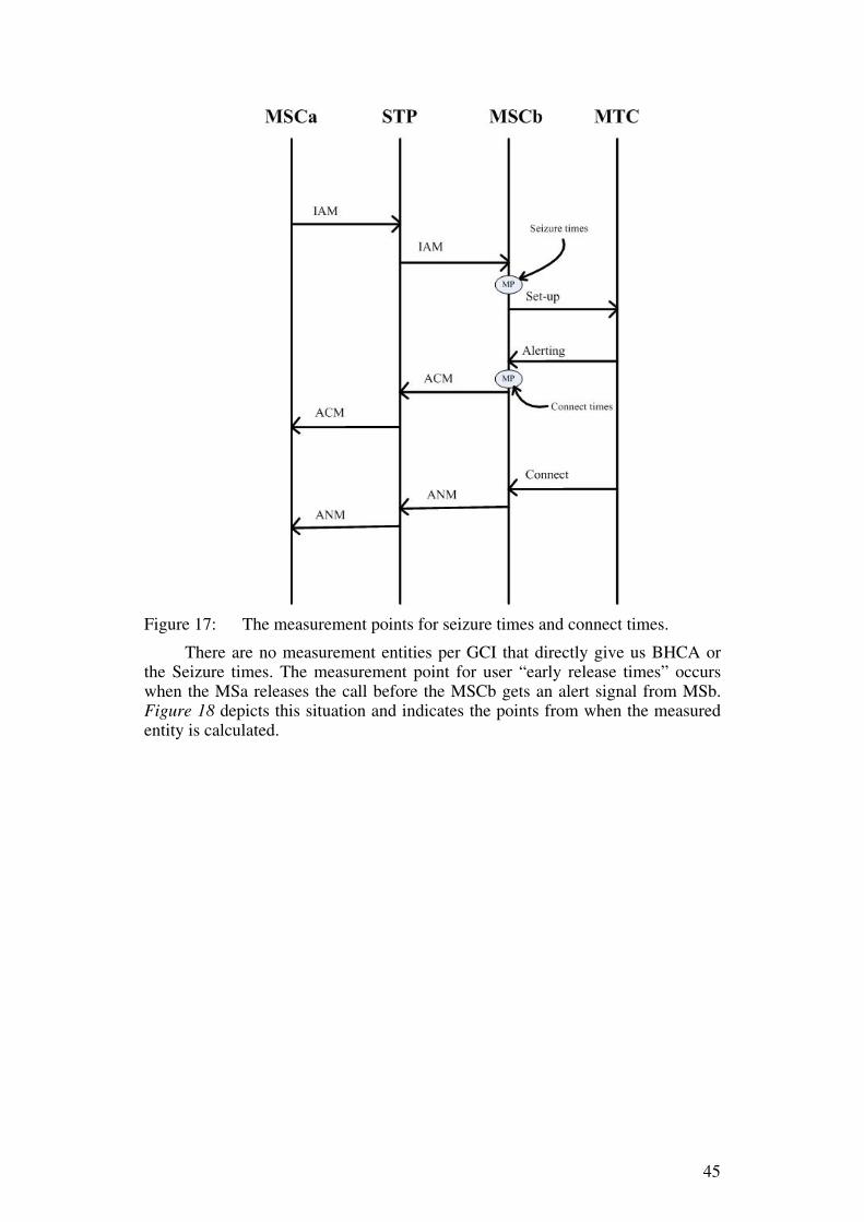
45
Figure 17: The measurement points for seizure times and connect times.
There are no measurement entities per GCI that directly give us BHCA or the Seizure times. The measurement point for user “early release times” occurs when the MSa releases the call before the MSCb gets an alert signal from MSb. Figure 18 depicts this situation and indicates the points from when the measured entity is calculated.
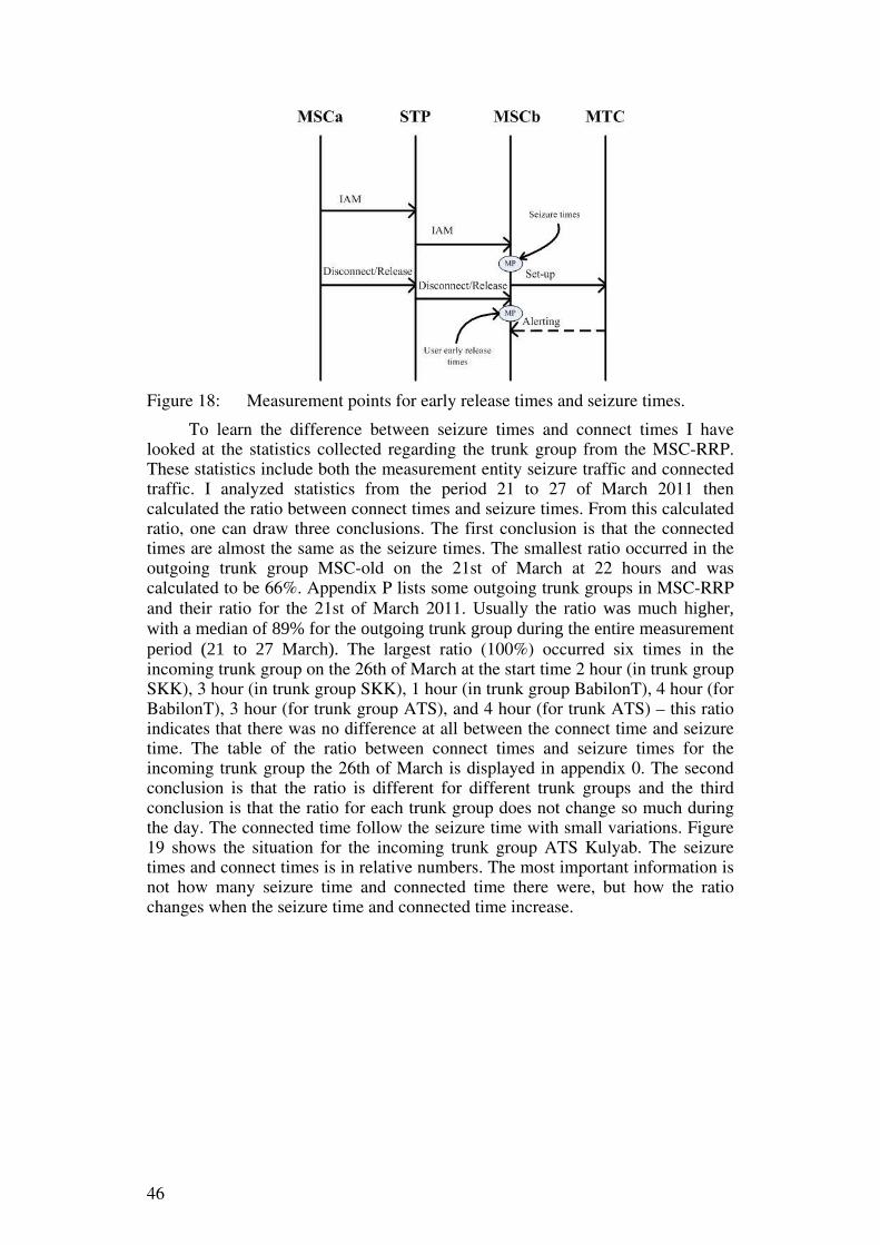
46
Figure 18: Measurement points for early release times and seizure times.
To learn the difference between seizure times and connect times I have looked at the statistics collected regarding the trunk group from the MSC-RRP. These statistics include both the measurement entity seizure traffic and connected traffic. I analyzed statistics from the period 21 to 27 of March 2011 then calculated the ratio between connect times and seizure times. From this calculated ratio, one can draw three conclusions. The first conclusion is that the connected times are almost the same as the seizure times. The smallest ratio occurred in the outgoing trunk group MSC-old on the 21st of March at 22 hours and was calculated to be 66%. Appendix P lists some outgoing trunk groups in MSC-RRP and their ratio for the 21st of March 2011. Usually the ratio was much higher, with a median of 89% for the outgoing trunk group during the entire measurement period (21 to 27 March). The largest ratio (100%) occurred six times in the incoming trunk group on the 26th of March at the start time 2 hour (in trunk group SKK), 3 hour (in trunk group SKK), 1 hour (in trunk group BabilonT), 4 hour (for BabilonT), 3 hour (for trunk group ATS), and 4 hour (for trunk ATS) – this ratio indicates that there was no difference at all between the connect time and seizure time. The table of the ratio between connect times and seizure times for the incoming trunk group the 26th of March is displayed in appendix 0. The second conclusion is that the ratio is different for different trunk groups and the third conclusion is that the ratio for each trunk group does not change so much during the day. The connected time follow the seizure time with small variations. Figure 19 shows the situation for the incoming trunk group ATS Kulyab. The seizure times and connect times is in relative numbers. The most important information is not how many seizure time and connected time there were, but how the ratio changes when the seizure time and connected time increase.
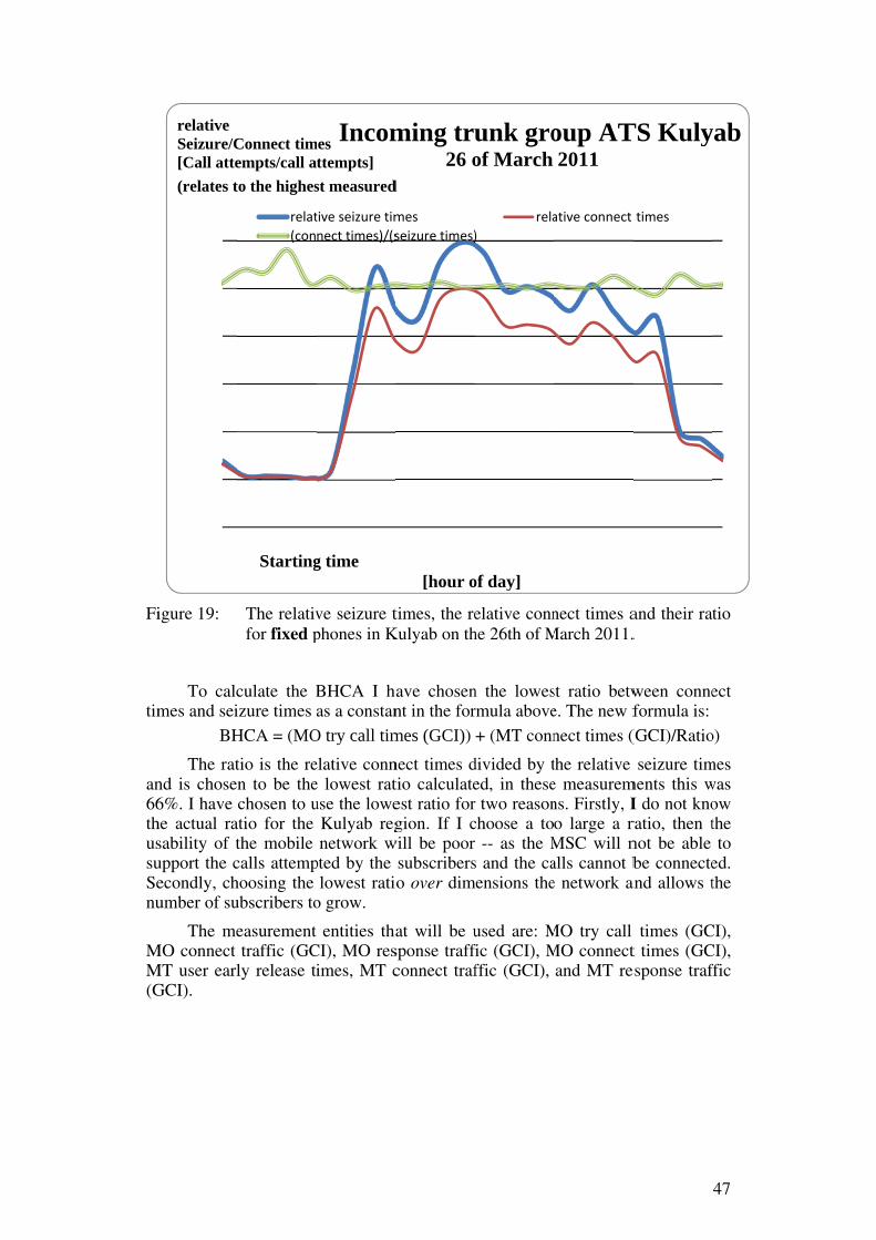
Fi
tim
an66thussuSenu
MM(G
igure 19:
To calcmes and sei
BH
The ratnd is chose6%. I have he actual rasability of tupport the cecondly, chumber of su
The meMO connect MT user earlGCI).
relativeSeizure/C[Call atte(relates t
The relativfor fixed p
culate the Bizure times HCA = (MOtio is the ren to be thechosen to u
atio for the the mobile calls attemphoosing the ubscribers to
easurement traffic (GC
ly release ti
Starting
relat(con
Connect timempts/call ato the highes
ve seizure tphones in K
BHCA I haas a constan
O try call timelative conne lowest ratuse the lowe
Kulyab regnetwork w
pted by the lowest ratio
o grow.
entities thaCI), MO resimes, MT c
g time
tive seizure timnect times)/(s
mes ttempts]st measured
Incom
times, the reKulyab on th
ave chosennt in the formes (GCI)) nect times dtio calculateest ratio forgion. If I c
will be poor subscriberso over dim
at will be usponse traffconnect traf
[hour o
messeizure times)
d
ming tru26 o
elative connhe 26th of M
n the lowesrmula above+ (MT conn
divided by ted, in theser two reasonchoose a to
-- as the Ms and the ca
mensions the
used are: Mfic (GCI), Mffic (GCI),
of day]
rela)
unk groof March
nect times aMarch 2011.
st ratio betwe. The new fnect times (
the relative e measuremns. Firstly, Io large a rMSC will nalls cannot be network an
MO try call MO connect
and MT re
ative connect
oup AT2011
and their ra.
ween conneformula is: (GCI)/Ratio
seizure timments this wI do not knoratio, then tnot be able be connecte
and allows t
times (GCt times (GCesponse traf
times
TS Kuly
47
tio
ect
o)
mes was ow the to
ed. the
CI), CI), ffic
yab

48
2.2.2.2. Calculation of BHCA for computing the capacity gain of the MSC-RRP
The parameters concerning the calculation of BHCA are different when collecting statistics from all base stations and when collecting statistics regarding GCI. The parameters used when collecting statistics from all base stations are 2G originating call attempt times and 2G terminated call attempts. MO try call times (GCI) and MT connected times (GCI) are used when collecting statistics regarding GCI.
The 2G originating call attempt is a parameter that measures each time the MSC receives a setup message from the MS [3]. The “equivalent” parameter used when collecting the statistics regarding GCI (the statistics collected regarding the LAC in Kulyab region) is the MO try call times. The MO try call times measures each time the MSC receives a CM_service_req message from BSC [3]. The figure below shows when these parameters are measured.
Figure 20: When the parameter 2G originating call attempts and MO try call
attempts are measured
The measure point for the 2G originating call attempts and MO try call
attempts occurs at the same point. That is good. It means that it is the same parameter, but have different names.
The parameter 2G terminated call attempt is a parameter that is measured each time the MSC receives a setup message from its BSC (intra-MSC call) or an IAI or an IAM message (inter- MSC) [3]. The “equivalent” parameter regarding GCI is MT connect times. This parameter measures each time the MSC receives an alerting message from the terminated MS [3]. The parameter calculating the MT part of the BHCA for MSC-RRP occurs much earlier in time than for the MSC in Kulyab. That means that the calculated BHCA value for MSC-RRP will have a much higher value that for the MSC in Kulyab. This means that the Kulyab will have a slight smaller value than it really has. So the MSC-RRP will have a slight better efficiently value than the thesis will show.
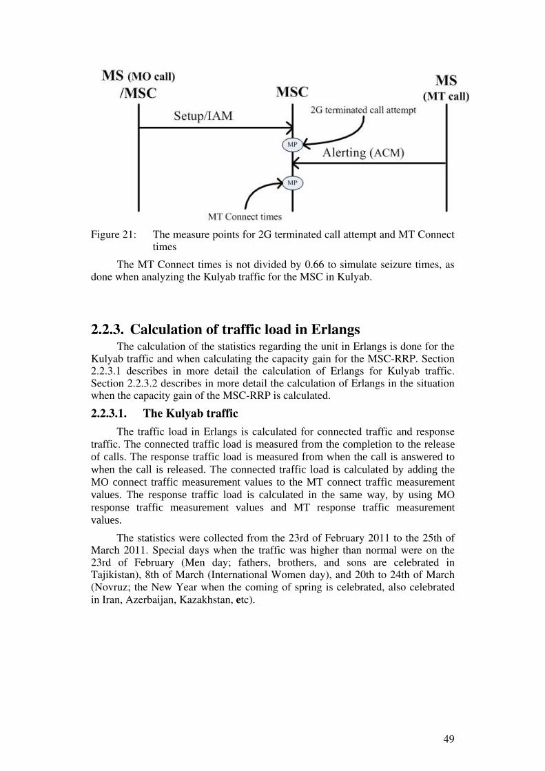
49
Figure 21: The measure points for 2G terminated call attempt and MT Connect
times
The MT Connect times is not divided by 0.66 to simulate seizure times, as done when analyzing the Kulyab traffic for the MSC in Kulyab.
2.2.3. Calculation of traffic load in Erlangs The calculation of the statistics regarding the unit in Erlangs is done for the
Kulyab traffic and when calculating the capacity gain for the MSC-RRP. Section 2.2.3.1 describes in more detail the calculation of Erlangs for Kulyab traffic. Section 2.2.3.2 describes in more detail the calculation of Erlangs in the situation when the capacity gain of the MSC-RRP is calculated.
2.2.3.1. The Kulyab traffic
The traffic load in Erlangs is calculated for connected traffic and response traffic. The connected traffic load is measured from the completion to the release of calls. The response traffic load is measured from when the call is answered to when the call is released. The connected traffic load is calculated by adding the MO connect traffic measurement values to the MT connect traffic measurement values. The response traffic load is calculated in the same way, by using MO response traffic measurement values and MT response traffic measurement values.
The statistics were collected from the 23rd of February 2011 to the 25th of March 2011. Special days when the traffic was higher than normal were on the 23rd of February (Men day; fathers, brothers, and sons are celebrated in Tajikistan), 8th of March (International Women day), and 20th to 24th of March (Novruz; the New Year when the coming of spring is celebrated, also celebrated in Iran, Azerbaijan, Kazakhstan, etc).
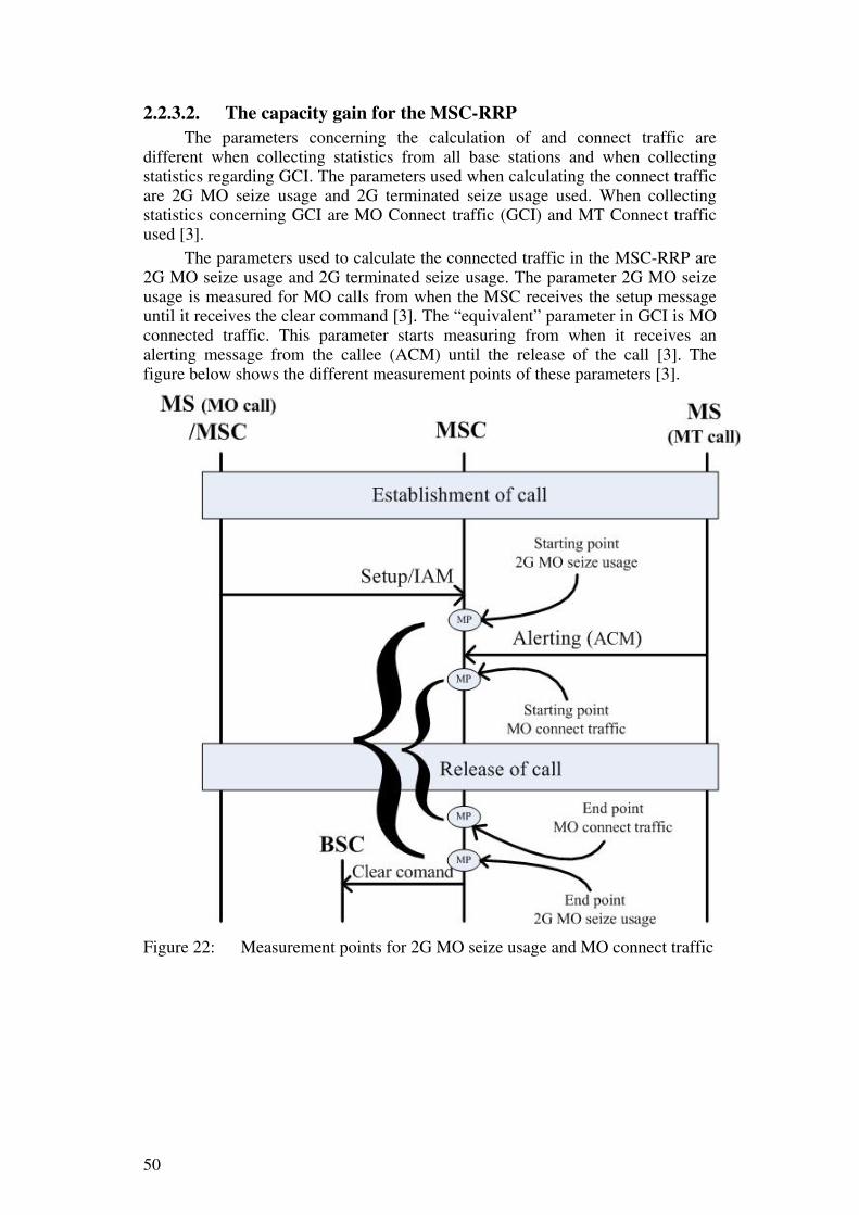
50
2.2.3.2. The capacity gain for the MSC-RRP The parameters concerning the calculation of and connect traffic are
different when collecting statistics from all base stations and when collecting statistics regarding GCI. The parameters used when calculating the connect traffic are 2G MO seize usage and 2G terminated seize usage used. When collecting statistics concerning GCI are MO Connect traffic (GCI) and MT Connect traffic used [3].
The parameters used to calculate the connected traffic in the MSC-RRP are 2G MO seize usage and 2G terminated seize usage. The parameter 2G MO seize usage is measured for MO calls from when the MSC receives the setup message until it receives the clear command [3]. The “equivalent” parameter in GCI is MO connected traffic. This parameter starts measuring from when it receives an alerting message from the callee (ACM) until the release of the call [3]. The figure below shows the different measurement points of these parameters [3].
Figure 22: Measurement points for 2G MO seize usage and MO connect traffic
51
The 2G seize usage has a measure point earlier than for the MO Connect traffic. This means that the 2G seize usage is bigger or equal to MO Connect traffic, thus Kulyab traffic will show a smaller percentage than it really has. This is not a problem. Then one knows that the capacity gain of the MSC-RRP will be bigger than it will show in the statistics. This in turn means that the remaining traffic load can grow at least as much as the Kulyab traffic load shows without any problems. If the Kulyab traffic load would show a bigger value than reality, then one would not be sure how much the remaining traffic load can increase.
The MT part of the calculation of the connect traffic for the MSC-RRP uses the parameter 2G terminated seize usage. The measuring starts after the call attempt is made and until the calls are released [3]. The “equivalent” parameter for GCI is MT Connect traffic. The measuring starts when the MSC receives an alerting message from the callee until the call is released [3]. These measure points occurs at the same time, see Figure 22 to see the measuring points.
The duration of the Kulyab traffic will show a smaller value than it really has. This follows the same argumentation as for the MO part of the connected traffic, thus the remaining traffic in MSC-RRP can grow at least as much as the Kulyab traffic shows without any problem.
2.2.4. Calculating the average call duration The average call duration is computed using Equation 1 and the parameters
respond traffic and respond times. Both of these parameters are measured when the callee picks up the call. The respond times measures how many times the call is responded and the respond traffic measures in Erlangs the duration of the call.
2.3. Analyzing strategy The analysis has been done for the Kulyab traffic as well as for the capacity
gain of MSC-RRP. Section 2.3.1 describes in more detail the analysis of Kulyab traffic. Section 2.3.2 describes in more detail the analysis of the capacity gain for MSC-RRP.
2.3.1. Analysis of the traffic in Kulyab The analysis of the traffic load for Kulyab region is done by collecting
statistics from LAC 0050 and 0051. These LACs are located in Khatlon province where Kulyab is situated. A more detailed list of the cells belonging to the two LACs are given in appendix D. The statistics are collected from the 23rd of February to the 25th of March 2011. All statistics throughout the report are shown as relative numbers. The statistics for the Kulyab region is analyzed for the whole period and for specific dates when the traffic is high. The statistics is displayed in graphs and tables. The highest measured value for each day is used to represent the traffic that day when analyzing statistics for the whole period. This means that the statistics for the whole period show the daily maximum value for each day in the period. The interesting parameters being analyzed are BHCA and connect traffic. When analyzing the traffic for one day, then the values for each hour will be used. Interesting parameters are BHCA, connected traffic, and response traffic. The average call duration will also be analyzed for the Kulyab traffic. This will also be done for the whole period and some interesting days when traffic is high.

52
The traffic will also be compared to the capacity of the MSC in Kulyab. Then the highest daily value will be used to compare with the capacity of the MSC. The interesting parameters are BHCA and connect traffic.
2.3.2. Analysis of the capacity gain for MSC-RRP The analysis of the performance efficiency for the MSC-RRP is also
analyzed. This is done by collecting statistics from the overall 2G traffic generated by the MSC-RRP. The measured period is from the 16th of May until the 22 of May 2011. The statistics concerning the Kulyab traffic were also collected during the same time period. The statistics are collected for each hour during the time period for the overall traffic in MSC-RRP and for the Kulyab traffic. The parameters of interest are BHCA and the connected traffic.
The capacity of the MSC-RRP is calculated regarding its capacity in BHCA and connected traffic. The increased capacity of the MSC-RRP is calculated using Equation 2 and also computed regarding BHCA and connected traffic.
The values used for calculating the increased capacity are the highest and lowest measured value for the Kulyab traffic.
The percentage of the traffic belonging to Kulyab will also be calculated. This thesis will show the result as a relative percentage. This will show how the Kulyab traffic changes over time.
The capacity gain for the MSC-RRP will be calculated for the highest measured Kulyab traffic load, the highest traffic load generated by all base stations in MSC-RRP, the highest percentage of Kulyab traffic when there is a peak in traffic, and the lowest percentage of Kulyab traffic when there is a peak in traffic.
The traffic volume for the total traffic in MSC-RRP is not shown at all in this report.
53
3. Analysis of the collected statistics and the maximum capacity of the MSC
The analysis is done for the collected statistics and for the calculated maximum capacity of the MSC as configured. Section 3.1 describes in more detail of the calculation and analysis of the MSC in Kulyab. Section 3.2 describes in more detail the analysis of the traffic flows in Kulyab area. Section 3.3 describes in more detail the analysis of the capacity gain for MSC-RRP. Section 3.4 has a general analysis and discusses a proposed solution.
3.1. Calculation and analysis of the MSC server and MGW hardware capacities in Kulyab
The calculation of the MSC hardware is done for the MSC server and for the MGW. Section 3.1.1 describe in more detail about the calculation of the maximum capacity of the MSC server as configured. Section 3.1.2 describe in more detail about the maximum capacity of the MGW as configured.
3.1.1. The MSC server in Kulyab The different boards in the MSC server were shown in Table 1 and Table 2
on page 26. The WCSU and WCCU were configured with the service processing software. These two types of boards perform signaling processing, call processing, mobility management, and resource management -- thus they determine the capacity of the MSC in terms of BHCA, the number of trunks, the number of 64 Kbit/s links, and the number of 2 Mbit/s links as shown in Table 11.

54
Table 11: The capacity of the MSC server according to the number of WCSUs and WCCUs (Note that the BHCA is a relative value. The relative BHCA value has been related to the highest BHCA value measured in the period 23rd of February to the 25th of March 2011)
Name of board WCSU WCCU Total Capacity (k)Total number of boards 2x 2y
Call processing capacityBHCA (per pair)
VMSC (k) 75 75GMSC (k) 160 160
Number of trunks (per pair)GMSC (k) 5 5
Number of 64 kbit/s links 32Number of 2 Mbit/s links 2
ResultTotal BHCA
VMSC (k) 0,590 2,444 3.034 [1]Total number of trunks
GMSC (k) 5x 5yTotal number of links
64 kbit/s 64x 64x2 Mbit/s 2x 2x
[1] Note that this value and all vales of BHCA and traffic intensity in the thesis work are relative numbers.
Table 11 shows that the MSC server in Kulyab has the relative capacity of 3.034 BHCA†† when acting as a VMSC (for internal mobile traffic).
†† Note that all values of BHCA and traffic intensity are relative numbers.
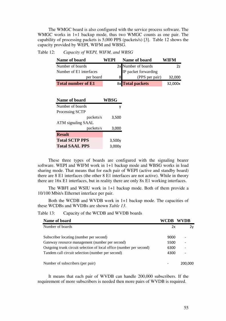
55
The WMGC board is also configured with the service process software. The WMGC works in 1+1 backup mode, thus two WMGC counts as one pair. The capability of processing packets is 5,000 PPS (packets/s) [3]. Table 12 shows the capacity provided by WEPI, WIFM and WBSG.
Table 12: Capacity of WEPI, WIFM, and WBSG
Name of board WEPI Name of board WIFMNumber of boards 2x Number of boards 2zNumber of E1 interfaces IP packet forwarding
per board 8 (PPS per pair) 32,000Total number of E1 8x Total packets 32,000x
Name of board WBSGNumber of boards yProcessing SCTP
packets/s 3,500ATM signaling SAAL
packets/s 3,000ResultTotal SCTP PPS 3,500yTotal SAAL PPS 3,000y
These three types of boards are configured with the signaling bearer software. WEPI and WIFM work in 1+1 backup mode and WBSG works in load sharing mode. That means that for each pair of WEPI (active and standby board) there are 8 E1 interfaces (the other 8 E1 interfaces are not active). While in theory there are 16x E1 interfaces, but in reality there are only 8x E1 working interfaces.
The WBFI and WSIU work in 1+1 backup mode. Both of them provide a 10/100 Mbit/s Ethernet interface per pair.
Both the WCDB and WVDB work in 1+1 backup mode. The capacities of these WCDBs and WVDBs are shown Table 13.
Table 13: Capacity of the WCDB and WVDB boards
Name of board WCDB WVDBNumber of boards 2x 2y
Subscriber locating (number per second) 9000 -Gateway resource management (number per second) 5500 -Outgoing trunk circuit selection of local office (number per second) 6300 -Tandem call circuit selection (number per second) 4300 -
Number of subscribers (per pair) - 200,000
It means that each pair of WVDB can handle 200,000 subscribers. If the
requirement of more subscribers is needed then more pairs of WVDB is required.
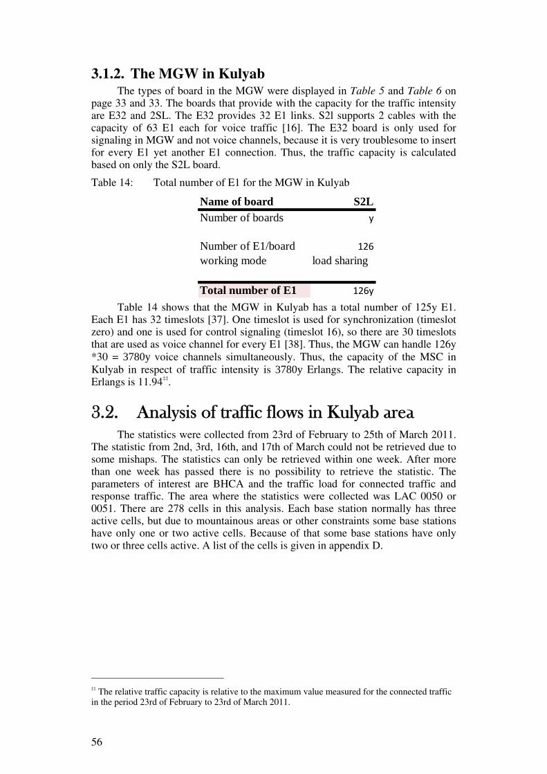
56
3.1.2. The MGW in Kulyab The types of board in the MGW were displayed in Table 5 and Table 6 on
page 33 and 33. The boards that provide with the capacity for the traffic intensity are E32 and 2SL. The E32 provides 32 E1 links. S2l supports 2 cables with the capacity of 63 E1 each for voice traffic [16]. The E32 board is only used for signaling in MGW and not voice channels, because it is very troublesome to insert for every E1 yet another E1 connection. Thus, the traffic capacity is calculated based on only the S2L board.
Table 14: Total number of E1 for the MGW in Kulyab
Name of board S2LNumber of boards y
Number of E1/board 126working mode load sharing
Total number of E1 126y Table 14 shows that the MGW in Kulyab has a total number of 125y E1.
Each E1 has 32 timeslots [37]. One timeslot is used for synchronization (timeslot zero) and one is used for control signaling (timeslot 16), so there are 30 timeslots that are used as voice channel for every E1 [38]. Thus, the MGW can handle 126y *30 = 3780y voice channels simultaneously. Thus, the capacity of the MSC in Kulyab in respect of traffic intensity is 3780y Erlangs. The relative capacity in Erlangs is 11.94‡‡.
3.2. Analysis of traffic flows in Kulyab area The statistics were collected from 23rd of February to 25th of March 2011.
The statistic from 2nd, 3rd, 16th, and 17th of March could not be retrieved due to some mishaps. The statistics can only be retrieved within one week. After more than one week has passed there is no possibility to retrieve the statistic. The parameters of interest are BHCA and the traffic load for connected traffic and response traffic. The area where the statistics were collected was LAC 0050 or 0051. There are 278 cells in this analysis. Each base station normally has three active cells, but due to mountainous areas or other constraints some base stations have only one or two active cells. Because of that some base stations have only two or three cells active. A list of the cells is given in appendix D.
‡‡ The relative traffic capacity is relative to the maximum value measured for the connected traffic in the period 23rd of February to 23rd of March 2011.

57
3.2.1. The evaluation process The values that are obtained from the statistics and from the calculation of
the capacity of the MSC in Kulyab have been expressed as relative numbers. This is to hide the details of the actual traffic in the Kulyab region. These statistics are expressed relative to be the highest measured value obtained from the BHCA traffic and the connect traffic in the period 23rd of February to the 25th of March 2011. The unit of the BHCA is call attempts. The unit for connect and response traffic is Erlangs. The relative values of BHCA and the traffic intensity are a percentage of the highest measured value for BCHA and Connect traffic. Therefore they cannot be expressed in Erlangs or call attempts, but rather expressed as a percentage of highest measured value (HMV). BHMV denotes the HMV for BHCA and CHMV denotes the HMV for connected traffic.
The capacity of the MSC in Kulyab is also described in relative values. The capacity of the MSC regarding BHCA is relative to the highest measured value of the BHCA traffic and the capacity of this MSC regarding traffic intensity is relative to the highest measured value of connected traffic.
The information obtained from the analysis was firstly analyzed for the whole period and then day by day. The information is displayed in charts to facilitate understanding of the traffic flow in Kulyab region.
The highest daily value of BHCA and connect traffic were chosen to represent the traffic for the actual day when analyzing statistic for the whole period. These values are displayed together in Graph 1. The response traffic will not be viewed as its behavior is similar to the behavior of connect traffic. The response traffic is also always lower than the connect traffic. This behavior of connect and response traffic can be viewed in
Graph 6. These two reasons make it more interesting to analyze the
parameter for connected traffic and for BHCA.
0
0.1
0.2
0.3
0.4
0.5
0.6
0.7
0.8
0.9
1
0 1 2 3 4 5 6 7 8 9 10 11 12 13 14 15 16 17 18 19 20 21 22 23
Rel
ativ
e tr
affic
load
Starting time of traffic [hour of day]
Traffic usagecollected the 23rd of February 2011
Relative connecttraffic
[Erlangs/Erlangs]

58
The measured statistics have also been compared with the capacity of the MSC in Kulyab.
The analysis starts with an analysis of the whole actual period.
3.2.2. Statistical analysis for the whole period (23rd of February to 25th of March 2011)
The measured values of the actual period regarding BHCA and connect traffic are given in appendix E and appendix F.
Graph 1 shows the maximum measured daily values regarding BHCA and connected traffic. The graph is based on the values from the table in appendix J. The dates missing are 2nd, 3rd, 16th, and 17th of March.
Graph 1: The maximum measured values for each day from the period 23rd
of February to the 25th of March 2011. NofA stands for relative number of attempts.
The graph shows that the traffic flow had two very big peaks, one on the 23rd of February (celebration of Men Day) and the other one in the 8th of March (celebration of International Women Day). Another smaller peak can been viewed at 22nd and 23rd of March when Novruz is celebrated. It is very interesting to see how well the traffic flow maps to the real world.
The plot also shows that the connected traffic more or less follows the value of BHCA. There are some variations when the traffic load rise, but the BHCA value decreases (27th of February and 23rd of March) and when the traffic intensity decreases and BHCA value increases (28th of February and 21st of March). A table with the daily maximum values for the whole measured period is given in appendix J.
Note that the Novruz-peak for BHCA took place the 22 of March and that the Novruz-peak for the connected traffic took place the 23rd of March. Section 3.2.3 will compare the traffic between those days and discuss this more deeply.
The average call duration for the whole period from the 23rd of February to the 25th of March 2011 is shown in
00.10.20.30.40.50.60.70.80.91
00.10.20.30.40.50.60.70.80.9
1
Feb. 23 25 27 March 1 3 5 7 9 11 13 15 17 19 21 23 25
Maximum connect traffic
(relates to CHMV)[Erlangs/Erlangs]
Maximum BHCA (relates to BHMV) [NofA/NofA]
Day of call attempts and connection traffic [month - day]
Maximum valuescollected from the 23rd of Feb. to 23rd of March 2011
Maximum BHCA Maximum connect traffic
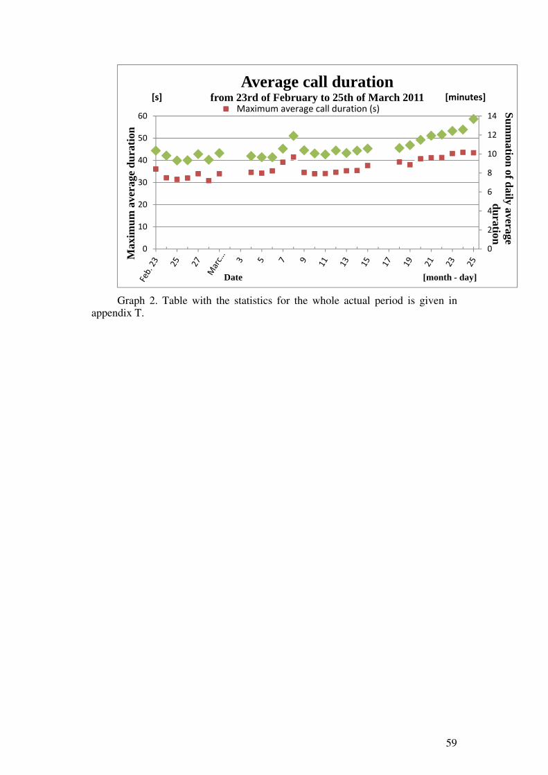
59
Graph 2. Table with the statistics for the whole actual period is given in
appendix T.
0
2
4
6
8
10
12
14
0
10
20
30
40
50
60
Summ
ation of daily average duration
Max
imum
ave
rage
dur
atio
n
Date [month - day]
Average call durationfrom 23rd of February to 25th of March 2011
Maximum average call duration (s)[s] [minutes]
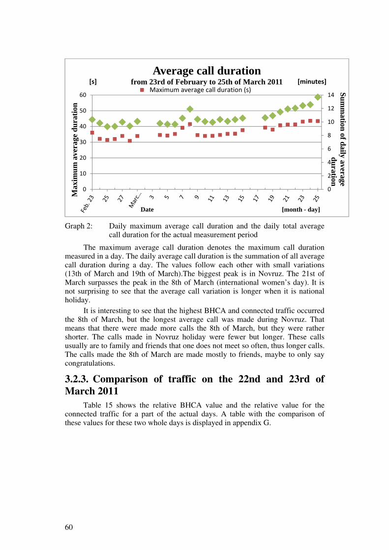
60
Graph 2: Daily maximum average call duration and the daily total average
call duration for the actual measurement period
The maximum average call duration denotes the maximum call duration measured in a day. The daily average call duration is the summation of all average call duration during a day. The values follow each other with small variations (13th of March and 19th of March).The biggest peak is in Novruz. The 21st of March surpasses the peak in the 8th of March (international women’s day). It is not surprising to see that the average call variation is longer when it is national holiday.
It is interesting to see that the highest BHCA and connected traffic occurred the 8th of March, but the longest average call was made during Novruz. That means that there were made more calls the 8th of March, but they were rather shorter. The calls made in Novruz holiday were fewer but longer. These calls usually are to family and friends that one does not meet so often, thus longer calls. The calls made the 8th of March are made mostly to friends, maybe to only say congratulations.
3.2.3. Comparison of traffic on the 22nd and 23rd of March 2011
Table 15 shows the relative BHCA value and the relative value for the connected traffic for a part of the actual days. A table with the comparison of these values for these two whole days is displayed in appendix G.
0
2
4
6
8
10
12
14
0
10
20
30
40
50
60
Summ
ation of daily average duration
Max
imum
ave
rage
dur
atio
n
Date [month - day]
Average call durationfrom 23rd of February to 25th of March 2011
Maximum average call duration (s)[s] [minutes]
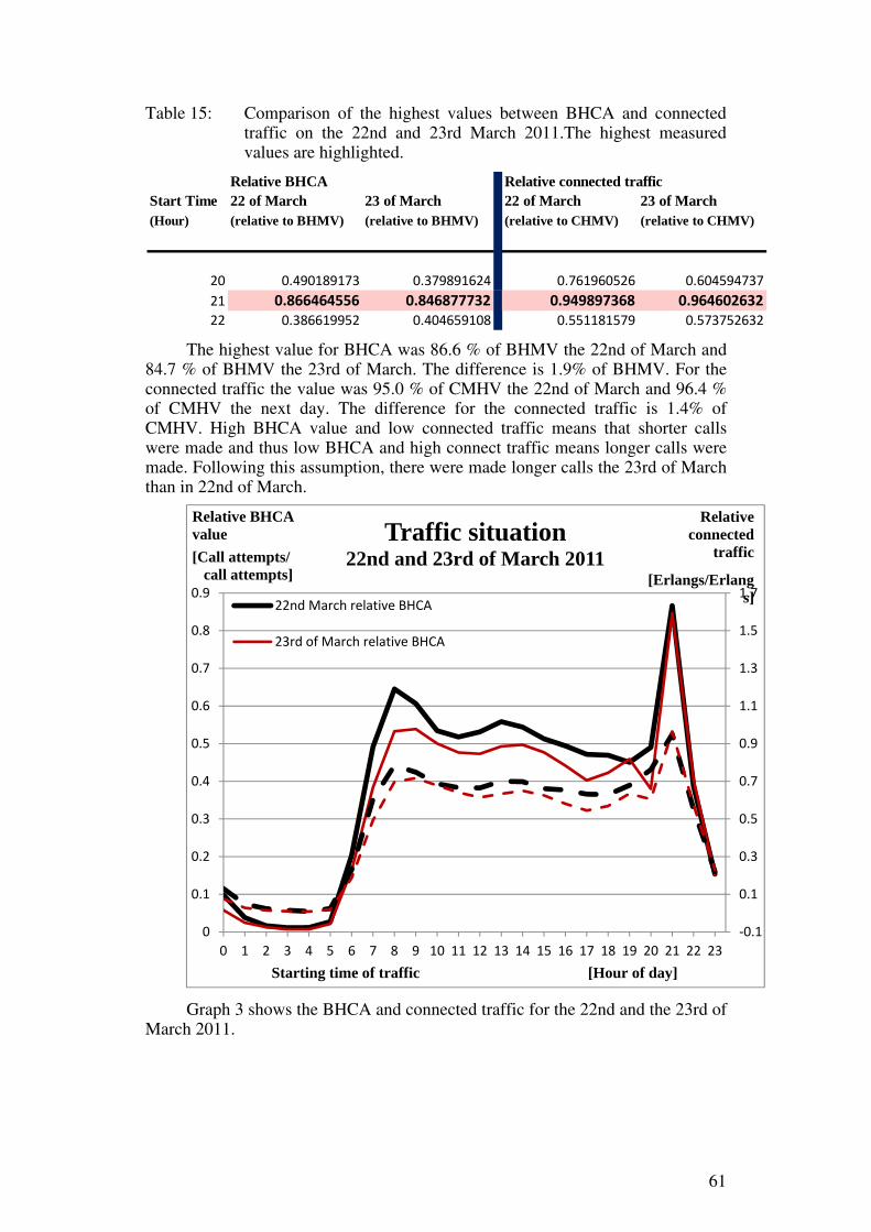
61
Table 15: Comparison of the highest values between BHCA and connected traffic on the 22nd and 23rd March 2011.The highest measured values are highlighted.
Start Time 22 of March 23 of March 22 of March 23 of March(Hour) (relative to BHMV) (relative to BHMV) (relative to CHMV) (relative to CHMV)
20 0.490189173 0.379891624 0.761960526 0.60459473721 0.866464556 0.846877732 0.949897368 0.96460263222 0.386619952 0.404659108 0.551181579 0.573752632
Relative BHCA Relative connected traffic
The highest value for BHCA was 86.6 % of BHMV the 22nd of March and 84.7 % of BHMV the 23rd of March. The difference is 1.9% of BHMV. For the connected traffic the value was 95.0 % of CMHV the 22nd of March and 96.4 % of CMHV the next day. The difference for the connected traffic is 1.4% of CMHV. High BHCA value and low connected traffic means that shorter calls were made and thus low BHCA and high connect traffic means longer calls were made. Following this assumption, there were made longer calls the 23rd of March than in 22nd of March.
Graph 3 shows the BHCA and connected traffic for the 22nd and the 23rd of
March 2011.
-0.1
0.1
0.3
0.5
0.7
0.9
1.1
1.3
1.5
1.7
0
0.1
0.2
0.3
0.4
0.5
0.6
0.7
0.8
0.9
0 1 2 3 4 5 6 7 8 9 10 11 12 13 14 15 16 17 18 19 20 21 22 23
Relative connected
traffic
[Erlangs/Erlangs]
Relative BHCA value[Call attempts/
call attempts]
Starting time of traffic [Hour of day]
Traffic situation22nd and 23rd of March 2011
22nd March relative BHCA
23rd of March relative BHCA

62
Graph 3: Comparison of BHCA and connect traffic for the 22nd and 23rd of
March.
The BHCA values for the 22nd and 23rd of March follow the same pattern as their connected traffic load as seen at
-0.1
0.1
0.3
0.5
0.7
0.9
1.1
1.3
1.5
1.7
0
0.1
0.2
0.3
0.4
0.5
0.6
0.7
0.8
0.9
0 1 2 3 4 5 6 7 8 9 10 11 12 13 14 15 16 17 18 19 20 21 22 23
Relative connected
traffic
[Erlangs/Erlangs]
Relative BHCA value[Call attempts/
call attempts]
Starting time of traffic [Hour of day]
Traffic situation22nd and 23rd of March 2011
22nd March relative BHCA
23rd of March relative BHCA

63
Graph 3.
-0.1
0.1
0.3
0.5
0.7
0.9
1.1
1.3
1.5
1.7
0
0.1
0.2
0.3
0.4
0.5
0.6
0.7
0.8
0.9
0 1 2 3 4 5 6 7 8 9 10 11 12 13 14 15 16 17 18 19 20 21 22 23
Relative connected
traffic
[Erlangs/Erlangs]
Relative BHCA value[Call attempts/
call attempts]
Starting time of traffic [Hour of day]
Traffic situation22nd and 23rd of March 2011
22nd March relative BHCA
23rd of March relative BHCA
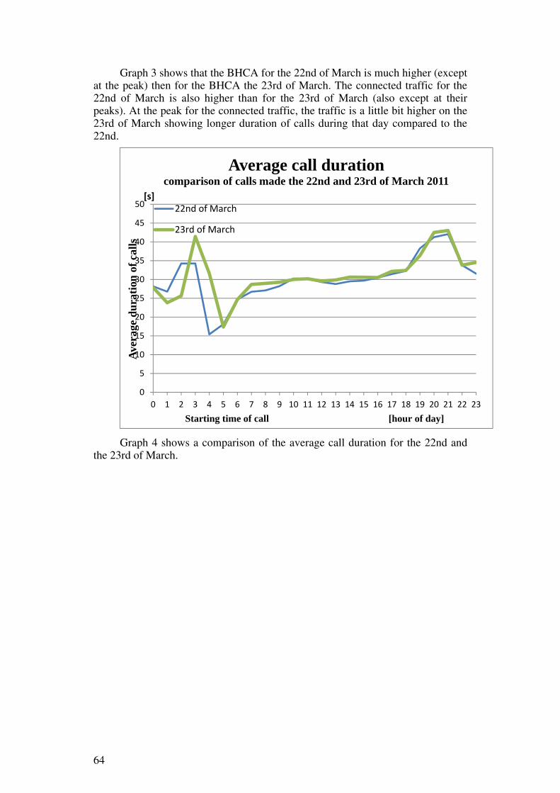
64
Graph 3 shows that the BHCA for the 22nd of March is much higher (except at the peak) then for the BHCA the 23rd of March. The connected traffic for the 22nd of March is also higher than for the 23rd of March (also except at their peaks). At the peak for the connected traffic, the traffic is a little bit higher on the 23rd of March showing longer duration of calls during that day compared to the 22nd.
Graph 4 shows a comparison of the average call duration for the 22nd and
the 23rd of March.
0
5
10
15
20
25
30
35
40
45
50
0 1 2 3 4 5 6 7 8 9 10 11 12 13 14 15 16 17 18 19 20 21 22 23
Aver
age
dura
tion
of c
alls
Starting time of call [hour of day]
Average call durationcomparison of calls made the 22nd and 23rd of March 2011
22nd of March
23rd of March
[s]

65
Graph 4: Comparison of the average call duration for the 22nd and 23rd of
March 2011.
The parameters MO respond traffic, MT respond traffic, MO respond times and MT respond times are used to calculate the call durations. The formula used is Equation 1 on page 37, for calculation of Erlangs.
0
5
10
15
20
25
30
35
40
45
50
0 1 2 3 4 5 6 7 8 9 10 11 12 13 14 15 16 17 18 19 20 21 22 23
Aver
age
dura
tion
of c
alls
Starting time of call [hour of day]
Average call durationcomparison of calls made the 22nd and 23rd of March 2011
22nd of March
23rd of March
[s]
0
5
10
15
20
25
30
35
40
45
50
0 1 2 3 4 5 6 7 8 9 10 11 12 13 14 15 16 17 18 19 20 21 22 23
Aver
age
dura
tion
of c
alls
Starting time of call [hour of day]
Average call durationcomparison of calls made the 22nd and 23rd of March 2011
22nd of March
23rd of March
[s]
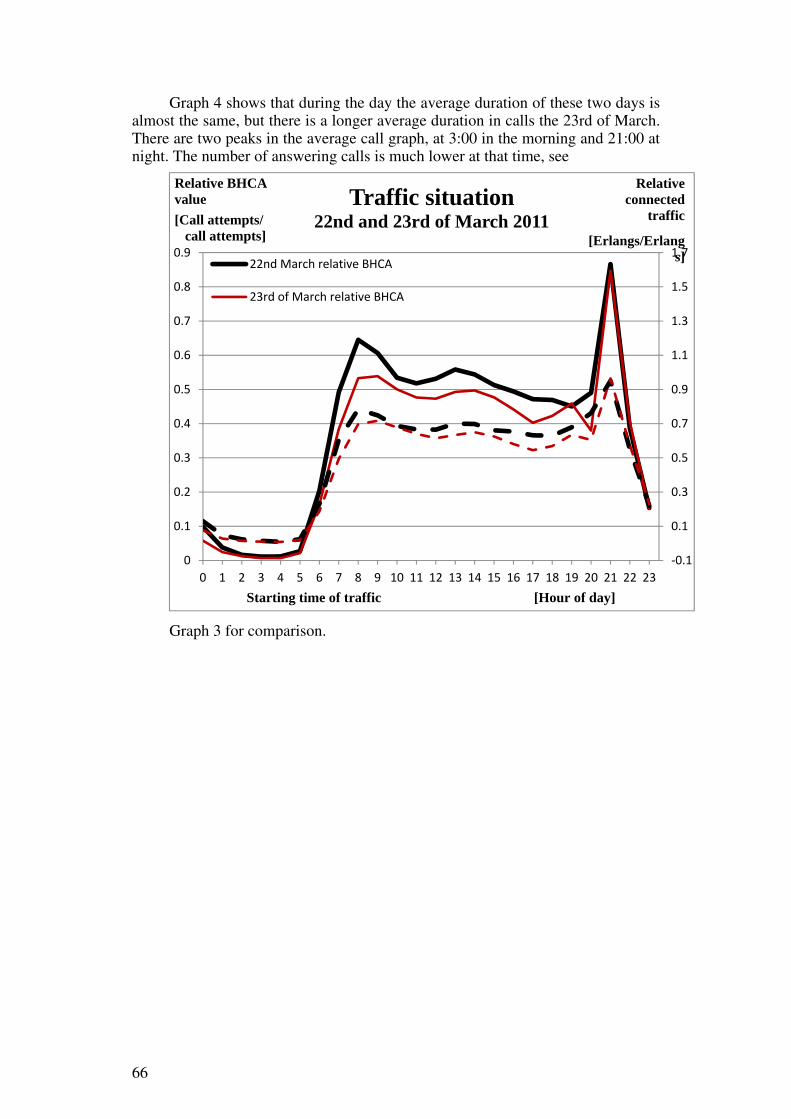
66
Graph 4 shows that during the day the average duration of these two days is almost the same, but there is a longer average duration in calls the 23rd of March. There are two peaks in the average call graph, at 3:00 in the morning and 21:00 at night. The number of answering calls is much lower at that time, see
Graph 3 for comparison.
-0.1
0.1
0.3
0.5
0.7
0.9
1.1
1.3
1.5
1.7
0
0.1
0.2
0.3
0.4
0.5
0.6
0.7
0.8
0.9
0 1 2 3 4 5 6 7 8 9 10 11 12 13 14 15 16 17 18 19 20 21 22 23
Relative connected
traffic
[Erlangs/Erlangs]
Relative BHCA value[Call attempts/
call attempts]
Starting time of traffic [Hour of day]
Traffic situation22nd and 23rd of March 2011
22nd March relative BHCA
23rd of March relative BHCA

67
3.2.4. Day by day statistics The highest traffic load occurs the 23rd of February and the 8th of March, as
shown in Graph 1. These days are interesting to view in more detail and will be analyzed in the sections below. The traffic for the 23rd of March will also be analyzed.
3.2.4.1. The 23rd of February
The results of the analysis of the statistics on the 23rd of February 2011 are given in appendix H. The relative BHCA value for the whole day is shown in
Graph 5 and the values for connect and response traffic are shown in
0
0.2
0.4
0.6
0.8
1
1.2
0 1 2 3 4 5 6 7 8 9 10 11 12 13 14 15 16 17 18 19 20 21 22 23
Rel
ativ
e B
HC
A
Starting time of traffic [Hour of day]
Relative BHCA Collected the 23rd of February 2011
relative BHCA
[Call attempts/call attempts

68
Graph 6.
0
0.1
0.2
0.3
0.4
0.5
0.6
0.7
0.8
0.9
1
0 1 2 3 4 5 6 7 8 9 10 11 12 13 14 15 16 17 18 19 20 21 22 23
Rel
ativ
e tr
affic
load
Starting time of traffic [hour of day]
Traffic usagecollected the 23rd of February 2011
Relative connecttraffic
[Erlangs/Erlangs]

69
Graph 5: Relative BHCA values for the 23rd of February 2011
Graph 6: Relative values for connect and response traffic on the 23rd of
February 2011
0
0.2
0.4
0.6
0.8
1
1.2
0 1 2 3 4 5 6 7 8 9 10 11 12 13 14 15 16 17 18 19 20 21 22 23
Rel
ativ
e B
HC
A
Starting time of traffic [Hour of day]
Relative BHCA Collected the 23rd of February 2011
relative BHCA
[Call attempts/call attempts
0
0.1
0.2
0.3
0.4
0.5
0.6
0.7
0.8
0.9
1
0 1 2 3 4 5 6 7 8 9 10 11 12 13 14 15 16 17 18 19 20 21 22 23
Rel
ativ
e tr
affic
load
Starting time of traffic [hour of day]
Traffic usagecollected the 23rd of February 2011
Relative connecttraffic
[Erlangs/Erlangs]

70
Graph 6 shows that the connect traffic and the response traffic have the
same behavior.
Graph 5 shows that the maximum value of BHCA occurs at 14 and
0
0.1
0.2
0.3
0.4
0.5
0.6
0.7
0.8
0.9
1
0 1 2 3 4 5 6 7 8 9 10 11 12 13 14 15 16 17 18 19 20 21 22 23
Rel
ativ
e tr
affic
load
Starting time of traffic [hour of day]
Traffic usagecollected the 23rd of February 2011
Relative connecttraffic
[Erlangs/Erlangs]
0
0.2
0.4
0.6
0.8
1
1.2
0 1 2 3 4 5 6 7 8 9 10 11 12 13 14 15 16 17 18 19 20 21 22 23
Rel
ativ
e B
HC
A
Starting time of traffic [Hour of day]
Relative BHCA Collected the 23rd of February 2011
relative BHCA
[Call attempts/call attempts

71
Graph 6 shows that the maximum traffic loads for both connect and
response traffic occurs at 20. Table 16 shows this more clearly. Table 16: Maximum value of BHCA and the maximum value of connect and
response traffic occurs at different hours the 23rd of February 2011
Starting time Relative Relative Relative BHCA connect traffic response traffic
(hour of day) (relates to BHMV) (relates to CHMV) (relates to CHMV)
(Call attempt/ call attempt)
13 0.8808 0.812037 0.58382914 0.970953 0.874711 0.63812415 0.937366 0.854321 0.62135816 0.910732 0.847811 0.61473717 0.890449 0.866279 0.63173418 0.782681 0.830142 0.60652419 0.685348 0.814387 0.61410320 0.849097 0.943913 0.74014221 0.800937 0.877997 0.696703
23rd of Feb. (Erlangs/Erlangs) (Erlangs/Erlangs)
The maximum BHCA occurs at 14:00 and has a value of 97.1 % of BHMV. The maximum traffic load occurs at 20:00. The connect traffic has a value of 94.4 % of CMHV and the response traffic has a value of 74.0 % of CMHV. When the traffic loads have their maximum peek, the BHCA has its second highest peak.
0
0.1
0.2
0.3
0.4
0.5
0.6
0.7
0.8
0.9
1
0 1 2 3 4 5 6 7 8 9 10 11 12 13 14 15 16 17 18 19 20 21 22 23
Rel
ativ
e tr
affic
load
Starting time of traffic [hour of day]
Traffic usagecollected the 23rd of February 2011
Relative connecttraffic
[Erlangs/Erlangs]

72
The value of BHCA is composed of “MO try call times” and “MT connect times divided by 0.66”. To understand why these maximums occur at different times, a comparison was made between MT connect times and MT connect traffic. A table with these values is given in appendix I.
Graph 7 shows the different patterns for MT connect times and MT connect
traffic.
0
0.1
0.2
0.3
0.4
0.5
0.6
00.020.040.060.080.1
0.120.140.160.180.2
0 1 2 3 4 5 6 7 8 9 10 11 12 13 14 15 16 17 18 19 20 21 22 23
MT connect traffic (relative value)M
T co
nnec
t tim
es (r
elat
ive
valu
e)
Starting time of traffic [Hour of day]
Different pattern between MT connect times and MT connect traffic
23rd of February 2011
MT connect timesMT connect traffic
[Connect attempts/connect attempts] [Erlangs/Erlangs]

73
Graph 7: Different patterns between relative connect times and relative
connect traffic for incoming traffic the 23rd of February 2011
As one can see from the
Graph 7, the MT connect times has the same pattern as the BHCA. The
maximum peak of the MT connect traffic occurs at 20:00 while the MT connect
0
0.1
0.2
0.3
0.4
0.5
0.6
00.020.040.060.080.1
0.120.140.160.180.2
0 1 2 3 4 5 6 7 8 9 10 11 12 13 14 15 16 17 18 19 20 21 22 23
MT connect traffic (relative value)M
T co
nnec
t tim
es (r
elat
ive
valu
e)
Starting time of traffic [Hour of day]
Different pattern between MT connect times and MT connect traffic
23rd of February 2011
MT connect timesMT connect traffic
[Connect attempts/connect attempts] [Erlangs/Erlangs]

74
times has a peak at 16:00. The different times of maximum may be due to the fact that at 16:00 when the incoming connect time was high the duration of incoming connect calls was not so long, perhaps because people were at work. However, at 20:00 the traffic load (MT connect traffic) was high, resulting in a peak. Appendix K lists the time when the BHCA peak occurs and also the peak for the traffic intensity for every day in the measured period. There is other days when the maximum peak of BHCA and connect traffic took place at different times in the day. Section 3.2.5 describes this situation in detail.
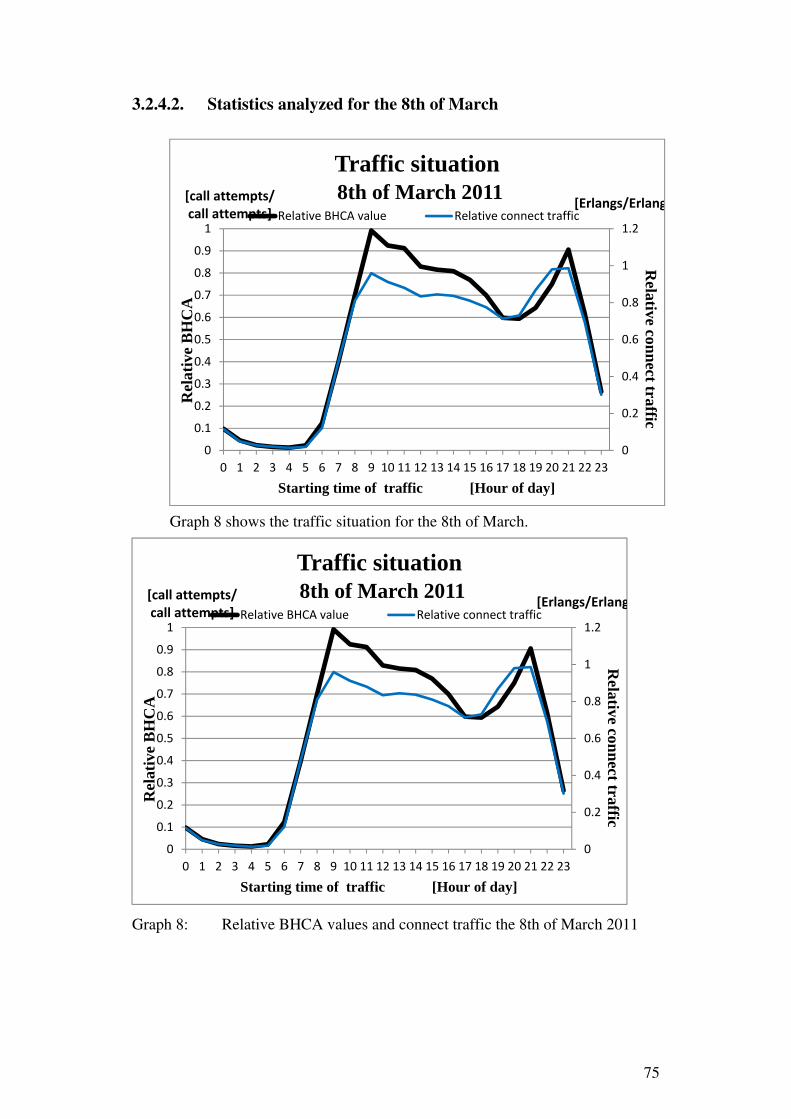
75
3.2.4.2. Statistics analyzed for the 8th of March
Graph 8 shows the traffic situation for the 8th of March.
Graph 8: Relative BHCA values and connect traffic the 8th of March 2011
0
0.2
0.4
0.6
0.8
1
1.2
0
0.1
0.2
0.3
0.4
0.5
0.6
0.7
0.8
0.9
1
0 1 2 3 4 5 6 7 8 9 10 11 12 13 14 15 16 17 18 19 20 21 22 23
Relative connect traffic
Rel
ativ
e B
HC
A
Starting time of traffic [Hour of day]
Traffic situation8th of March 2011
Relative BHCA value Relative connect traffic[call attempts/call attempts]
[Erlangs/Erlang
0
0.2
0.4
0.6
0.8
1
1.2
0
0.1
0.2
0.3
0.4
0.5
0.6
0.7
0.8
0.9
1
0 1 2 3 4 5 6 7 8 9 10 11 12 13 14 15 16 17 18 19 20 21 22 23
Relative connect traffic
Rel
ativ
e B
HC
A
Starting time of traffic [Hour of day]
Traffic situation8th of March 2011
Relative BHCA value Relative connect traffic[call attempts/call attempts]
[Erlangs/Erlang

76
The 8th of March 2011 was the highest value measured for both BHCA and connect traffic load. The maximum peak for BHCA occurred very early, at 9:00 in the morning. This is the earliest maximum peak measured during the entire measurement. Note that this day is the International Women Day, a holiday and not a working day.
Graph 8 shows that the curves of BHCA and connect traffic follow each
other, when BHCA increases the connect traffic also increases. The connect traffic has a plateau at its maximum peak. The BHCA increases in that peak. Thus the signaling increases, but the traffic is the same. This means that the traffic consists of shorter calls.
Each call is governed by control signaling. When a lot of calls start then a control signaling is needed leading to increased BHCA. The amount of control signaling is the same for a short and a long call. When a call is answered and not terminated, there is no need for control signaling. When the call is terminated, control signaling is used to terminate the call. Thus, a long call and a short call have the same total amount of control signaling [10]. The difference between a short call and a call with long duration is the traffic load in Erlangs. The BHCA due to control signaling is the same.
3.2.4.3. Statistics analyzed for the 22nd of March
0
0.2
0.4
0.6
0.8
1
1.2
0
0.1
0.2
0.3
0.4
0.5
0.6
0.7
0.8
0.9
1
0 1 2 3 4 5 6 7 8 9 10 11 12 13 14 15 16 17 18 19 20 21 22 23
Relative connect traffic
Rel
ativ
e B
HC
A
Starting time of traffic [Hour of day]
Traffic situation8th of March 2011
Relative BHCA value Relative connect traffic[call attempts/call attempts]
[Erlangs/Erlang
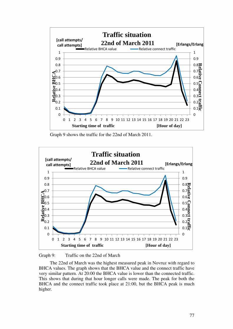
77
Graph 9 shows the traffic for the 22nd of March 2011.
Graph 9: Traffic on the 22nd of March
The 22nd of March was the highest measured peak in Novruz with regard to BHCA values. The graph shows that the BHCA value and the connect traffic have very similar pattern. At 20:00 the BHCA value is lower than the connected traffic. This shows that during that hour longer calls were made. The peak for both the BHCA and the connect traffic took place at 21:00, but the BHCA peak is much higher.
00.10.20.30.40.50.60.70.80.91
00.10.20.30.40.50.60.70.80.9
1
0 1 2 3 4 5 6 7 8 9 10 11 12 13 14 15 16 17 18 19 20 21 22 23
Relative C
onnect traffic
Rel
ativ
e B
HC
A
Starting time of traffic [Hour of day]
Traffic situation22nd of March 2011
Relative BHCA value Relative connect traffic
[call attempts/call attempts] [Erlangs/Erlangs
00.10.20.30.40.50.60.70.80.91
00.10.20.30.40.50.60.70.80.9
1
0 1 2 3 4 5 6 7 8 9 10 11 12 13 14 15 16 17 18 19 20 21 22 23
Relative C
onnect trafficR
elat
ive
BH
CA
Starting time of traffic [Hour of day]
Traffic situation22nd of March 2011
Relative BHCA value Relative connect traffic
[call attempts/call attempts] [Erlangs/Erlangs

78
3.2.5. Different peaks in time for BHCA and connect traffic in the same day
There are 18 days out of 27 when the peak of BHCA and the peak of the traffic load occur at the same hour. On the other nine days the peak occurs at different times. There are two types of situations when the peak occurs at different times: when the maximum peak occurs after a large interval in time and when the maximum peak occurs the next hour.
Of these nine days there are three days when the maximum value occurs at a large difference in time (23rd of February, 25th of February and 8th of March), as shown in Table 17.
Table 17: Maximum peak difference in time
Start Time BHCA Connect traffic Response traffic(relates to BHMV) (relates to CHMV)
(Hour) (Call attempts) (Erlangs)
February 23rd 14 0.970953 0.874711 0.63812420 0.849097 0.943913 0.740142
25th 15 0.713721 0.759455 0.56254720 0.679059 0.85905 0.689482
26th 15 0.663194 0.726018 0.53706820 0.613433 0.800039 0.636561
March 8th 9 0.991592 0.959039 0.71718421 0.905564 0.986016 0.774966
Date
(relates to CHMV)
(Erlangs)
These days have two peaks in traffic, one maximum peak and one that is the second highest peak. When the BHCA has its maximum peak then the connected traffic and the response traffic have their second highest peak. When connected and response traffic load have their maximum peak then the BHCA has its second highest peak.
The other six days have, with respect to relative BHCA traffic and relative connected traffic, their maximum peak with an hour apart from each other. Table 18 shows this situation.
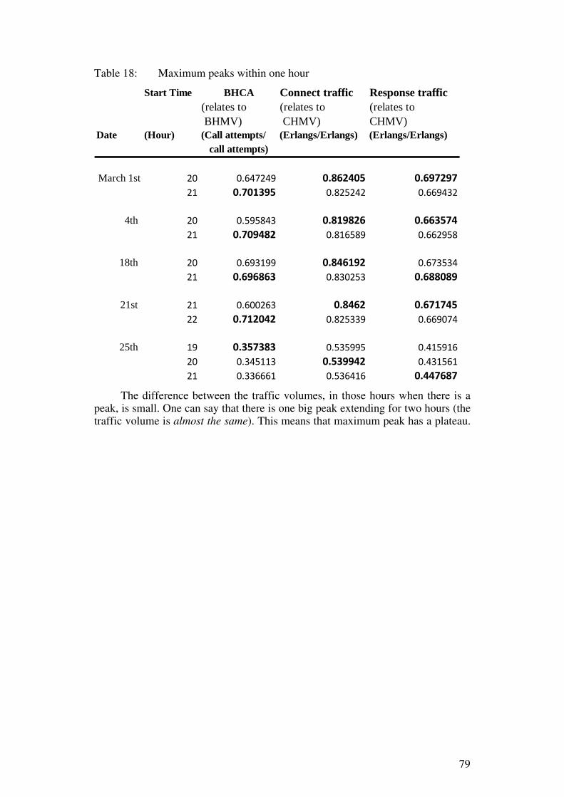
79
Table 18: Maximum peaks within one hour
Start Time BHCA Connect traffic Response traffic(relates to (relates to (relates to BHMV) CHMV) CHMV)
(Hour) (Call attempts/ (Erlangs/Erlangs) (Erlangs/Erlangs) call attempts)
March 1st 20 0.647249 0.862405 0.69729721 0.701395 0.825242 0.669432
4th 20 0.595843 0.819826 0.66357421 0.709482 0.816589 0.662958
18th 20 0.693199 0.846192 0.67353421 0.696863 0.830253 0.688089
21st 21 0.600263 0.8462 0.67174522 0.712042 0.825339 0.669074
25th 19 0.357383 0.535995 0.41591620 0.345113 0.539942 0.43156121 0.336661 0.536416 0.447687
Date
The difference between the traffic volumes, in those hours when there is a
peak, is small. One can say that there is one big peak extending for two hours (the traffic volume is almost the same). This means that maximum peak has a plateau.

80
A chart showing these two situations illustrates it better.
Graph 10 shows the BHCA traffic when there is an interval in time between
maximum peaks for BHCA traffic and connect traffic.
0
0.2
0.4
0.6
0.8
1
1.2
0 1 2 3 4 5 6 7 8 9 10 11 12 13 14 15 16 17 18 19 20 21 22 23
Rel
ativ
e B
HC
A v
alue
Starting time of call attempts [Hour of day]
Early maximum peakBHCA
statistics collected in 2011
23rd of February
25th of February 2011
26th of February
8th of March
[Call attempts/call attempts]

81
Graph 10: Early maximum peak for relative BHCA traffic
0
0.2
0.4
0.6
0.8
1
1.2
0 1 2 3 4 5 6 7 8 9 10 11 12 13 14 15 16 17 18 19 20 21 22 23
Rel
ativ
e B
HC
A v
alue
Starting time of call attempts [Hour of day]
Early maximum peakBHCA
statistics collected in 2011
23rd of February
25th of February 2011
26th of February
8th of March
[Call attempts/call attempts]

82
The
Graph 10 shows that all lines have at least two peaks. The line showing the
8th of March differs, but one can distinguish a third small peak that extends from 12:00 to 17:00. The maximum peak on the 8th of March has its maximum value at 9:00 and the second highest peak has its maximum value at 21:00.
The other days have more or less the same shape. One can distinguish three peaks. The peak in the middle is the highest peak. The second highest peak occurs always later and thus the third highest peak occurs earlier that day.
0
0.2
0.4
0.6
0.8
1
1.2
0 1 2 3 4 5 6 7 8 9 10 11 12 13 14 15 16 17 18 19 20 21 22 23
Rel
ativ
e B
HC
A v
alue
Starting time of call attempts [Hour of day]
Early maximum peakBHCA
statistics collected in 2011
23rd of February
25th of February 2011
26th of February
8th of March
[Call attempts/call attempts]
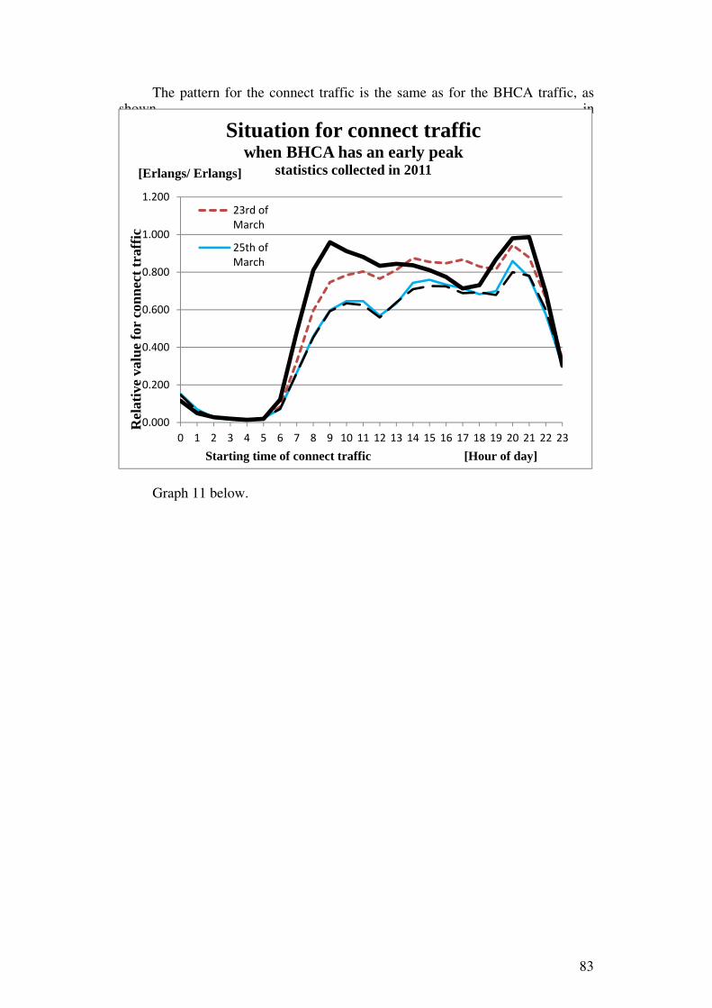
83
The pattern for the connect traffic is the same as for the BHCA traffic, as shown in
Graph 11 below.
0.000
0.200
0.400
0.600
0.800
1.000
1.200
0 1 2 3 4 5 6 7 8 9 10 11 12 13 14 15 16 17 18 19 20 21 22 23
Rel
ativ
e va
lue
for
conn
ect t
raff
ic
Starting time of connect traffic [Hour of day]
Situation for connect traffic when BHCA has an early peak
statistics collected in 2011
23rd ofMarch
25th ofMarch
[Erlangs/ Erlangs]
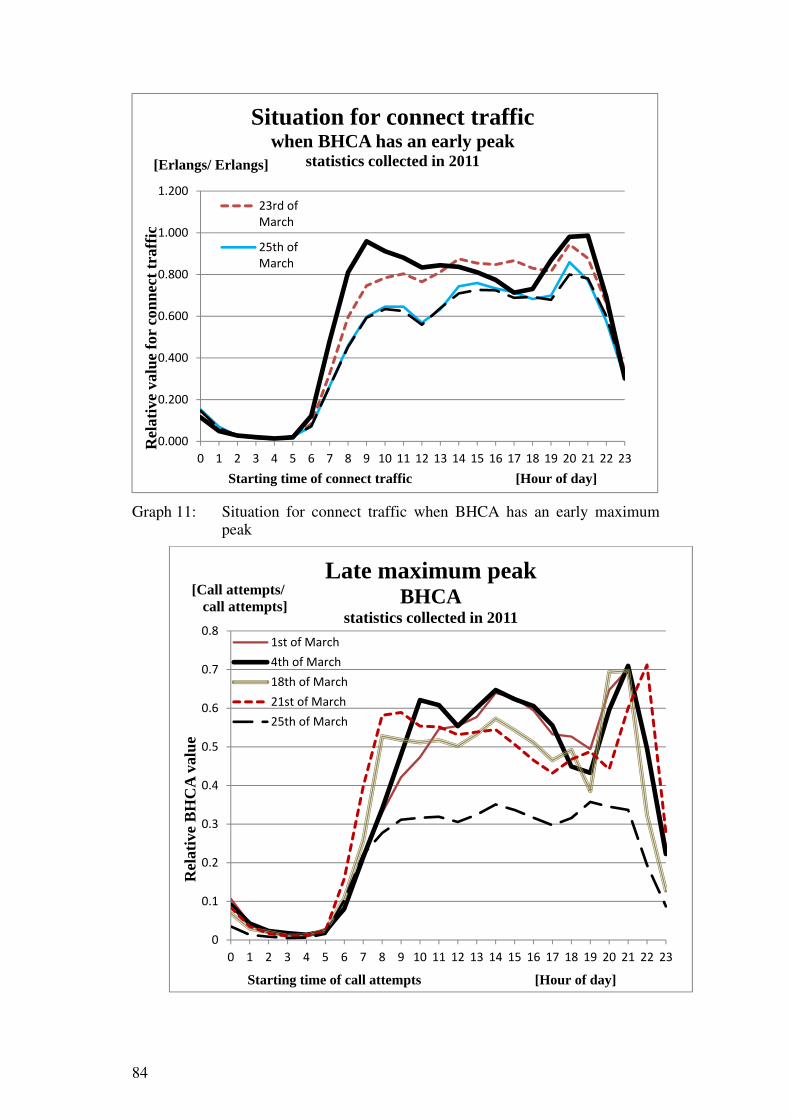
84
Graph 11: Situation for connect traffic when BHCA has an early maximum
peak
0.000
0.200
0.400
0.600
0.800
1.000
1.200
0 1 2 3 4 5 6 7 8 9 10 11 12 13 14 15 16 17 18 19 20 21 22 23
Rel
ativ
e va
lue
for
conn
ect t
raff
ic
Starting time of connect traffic [Hour of day]
Situation for connect traffic when BHCA has an early peak
statistics collected in 2011
23rd ofMarch
25th ofMarch
[Erlangs/ Erlangs]
0
0.1
0.2
0.3
0.4
0.5
0.6
0.7
0.8
0 1 2 3 4 5 6 7 8 9 10 11 12 13 14 15 16 17 18 19 20 21 22 23
Rel
ativ
e B
HC
A v
alue
Starting time of call attempts [Hour of day]
Late maximum peakBHCA
statistics collected in 20111st of March4th of March18th of March21st of March25th of March
[Call attempts/call attempts]

85
Graph 12 shows the situation for BHCA when the BHCA and connected traffic have their maximum peaks with an hour apart of each other.
Graph 12: BHCA values with a late maximum peak
The difference between this situation and the previous one is that the maximum peak for the BHCA occurs later. The traffic on the 25th of March is low, maybe due to the fact that the busy calling day of Novruz has passed (the traffic for connect traffic is also low). The pattern for the 25th of March also shows low variation in traffic. One can distinguish a plateau at the maximum peak
0
0.1
0.2
0.3
0.4
0.5
0.6
0.7
0.8
0 1 2 3 4 5 6 7 8 9 10 11 12 13 14 15 16 17 18 19 20 21 22 23
Rel
ativ
e B
HC
A v
alue
Starting time of call attempts [Hour of day]
Late maximum peakBHCA
statistics collected in 20111st of March4th of March18th of March21st of March25th of March
[Call attempts/call attempts]
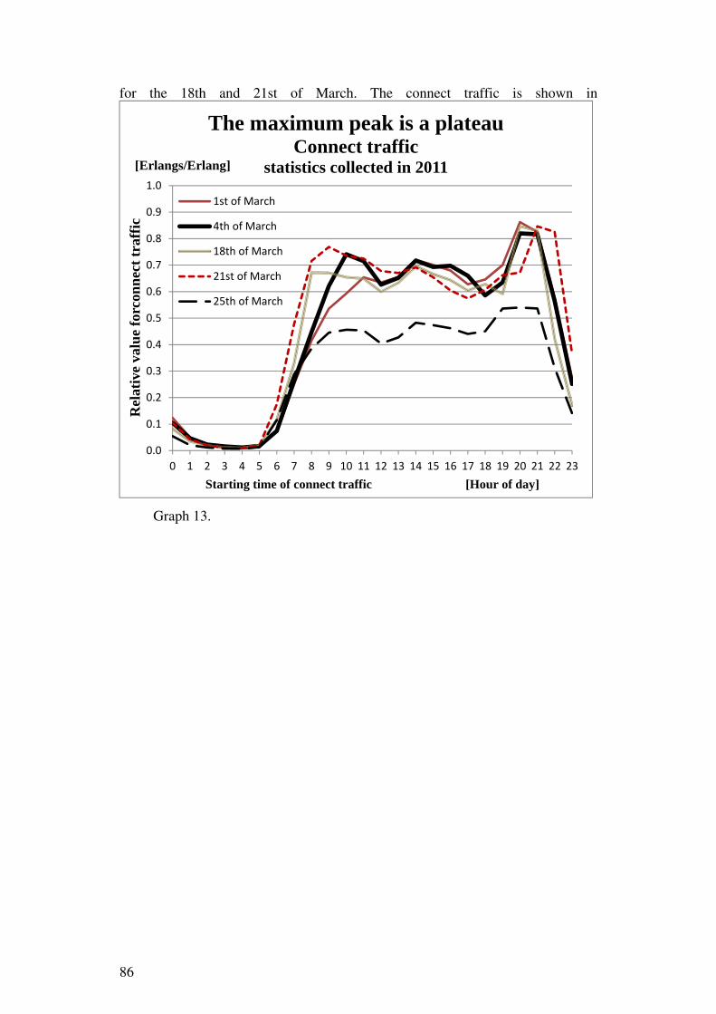
86
for the 18th and 21st of March. The connect traffic is shown in
Graph 13.
0.0
0.1
0.2
0.3
0.4
0.5
0.6
0.7
0.8
0.9
1.0
0 1 2 3 4 5 6 7 8 9 10 11 12 13 14 15 16 17 18 19 20 21 22 23
Rel
ativ
e va
lue
forc
onne
ct tr
affic
Starting time of connect traffic [Hour of day]
The maximum peak is a plateauConnect traffic
statistics collected in 2011
1st of March
4th of March
18th of March
21st of March
25th of March
[Erlangs/Erlang]

87
Graph 13: Connect traffic with a plateau in the maximum peak
0.0
0.1
0.2
0.3
0.4
0.5
0.6
0.7
0.8
0.9
1.0
0 1 2 3 4 5 6 7 8 9 10 11 12 13 14 15 16 17 18 19 20 21 22 23
Rel
ativ
e va
lue
forc
onne
ct tr
affic
Starting time of connect traffic [Hour of day]
The maximum peak is a plateauConnect traffic
statistics collected in 2011
1st of March
4th of March
18th of March
21st of March
25th of March
[Erlangs/Erlang]
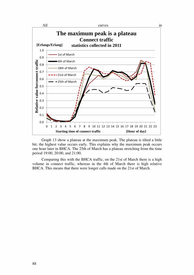
88
All curves in
Graph 13 show a plateau at the maximum peak. The plateau is tilted a little
bit; the highest value occurs early. This explains why the maximum peak occurs one hour later in BHCA. The 25th of March has a plateau stretching from the time period 19:00, 20:00, and 21:00.
Comparing this with the BHCA traffic, on the 21st of March there is a high volume in connect traffic, whereas in the 4th of March there is high relative BHCA. This means that there were longer calls made on the 21st of March.
0.0
0.1
0.2
0.3
0.4
0.5
0.6
0.7
0.8
0.9
1.0
0 1 2 3 4 5 6 7 8 9 10 11 12 13 14 15 16 17 18 19 20 21 22 23
Rel
ativ
e va
lue
forc
onne
ct tr
affic
Starting time of connect traffic [Hour of day]
The maximum peak is a plateauConnect traffic
statistics collected in 2011
1st of March
4th of March
18th of March
21st of March
25th of March
[Erlangs/Erlang]

89
3.2.6. More analysis regarding average call duration Appendix Q gives the statistic of the average call duration for each day and
each hour. The average call duration during a day follows almost the same pattern as
for BHCA traffic. The graph below shows when the average call duration shows a common pattern.
Graph 14: Average call duration for Kulyab traffic the 12th of March 2011
0.0
5.0
10.0
15.0
20.0
25.0
30.0
35.0
40.0
0 1 2 3 4 5 6 7 8 9 10 11 12 13 14 15 16 17 18 19 20 21 22 23
Cal
l dur
atio
n
Starting time of calls [hour of day]
Average call duration12th of March 2011
average call duration
[s]
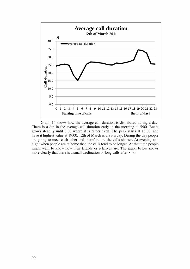
90
Graph 14 shows how the average call duration is distributed during a day.
There is a dip in the average call duration early in the morning at 5:00. But it grows steadily until 8:00 where it is rather even. The peak starts at 18:00, and have it highest value at 19:00. 12th of March is a Saturday. During the day people are going to meet each other and therefore are the calls shorter. At evening and night when people are at home then the calls tend to be longer. At that time people might want to know how their friends or relatives are. The graph below shows more clearly that there is a small declination of long calls after 8:00.
0.0
5.0
10.0
15.0
20.0
25.0
30.0
35.0
40.0
0 1 2 3 4 5 6 7 8 9 10 11 12 13 14 15 16 17 18 19 20 21 22 23
Cal
l dur
atio
n
Starting time of calls [hour of day]
Average call duration12th of March 2011
average call duration
[s]

91
Graph 15: Average call duration the 26th of February 2011
The average call duration on the 26th of February shows clearly that there are two peaks, one early in the morning and the other one at evening. There is a small peak very early in the morning at 4:00.
0.0
5.0
10.0
15.0
20.0
25.0
30.0
35.0
0 1 2 3 4 5 6 7 8 9 10 11 12 13 14 15 16 17 18 19 20 21 22 23
Cal
l dur
atio
n
Starting time of calls [hour of day]
Average call duration26th of February 2011
average call duration
[s]

92
A very unusual graph is depicted in
Graph 16. It is for the average call duration on the 23rd of March 2011. It is
a Wednesday in Novruz holiday.
0.0
5.0
10.0
15.0
20.0
25.0
30.0
35.0
40.0
45.0
50.0
0 1 2 3 4 5 6 7 8 9 1011121314151617181920212223
Cal
l dur
atio
n
Starting time of calls [hour of day]
Average call duration23rd of March 2011
average call duration
[s]

93
Graph 16: Average call duration the 23rd of March 2011
0.0
5.0
10.0
15.0
20.0
25.0
30.0
35.0
40.0
45.0
50.0
0 1 2 3 4 5 6 7 8 9 1011121314151617181920212223
Cal
l dur
atio
n
Starting time of calls [hour of day]
Average call duration23rd of March 2011
average call duration
[s]
0.0
5.0
10.0
15.0
20.0
25.0
30.0
35.0
40.0
45.0
50.0
0 1 2 3 4 5 6 7 8 9 1011121314151617181920212223
Cal
l dur
atio
n
Starting time of calls [hour of day]
Average call duration23rd of March 2011
average call duration
[s]

94
Graph 16 shows two very big peaks. The maximum peak has its maximum value at 21:00 in the evening. The second peak has its maximum value at 3:00 early in the morning. This pattern is very unusual. The 22nd of March has also a secondary big peak at that time early in the morning. Some dates show small tendency of a peak in the morning (26th of February, 28th of February, 4th of March, 5th of March, 7th of March, 8th of March, 9th of March, 14th of March, 15th of March, 18th of March, and 19th of March).
Graph 15 on page 91 shows for the 26th of February a small tendency of a
peak in the morning. The peak in the morning occurs when the BHCA traffic is low. This means
that almost all call attempts made in that time were responded and spoken for a rather long time. Maybe the call was international. More analysis has to be done to answer this question.
0.0
5.0
10.0
15.0
20.0
25.0
30.0
35.0
0 1 2 3 4 5 6 7 8 9 10 11 12 13 14 15 16 17 18 19 20 21 22 23
Cal
l dur
atio
n
Starting time of calls [hour of day]
Average call duration26th of February 2011
average call duration
[s]
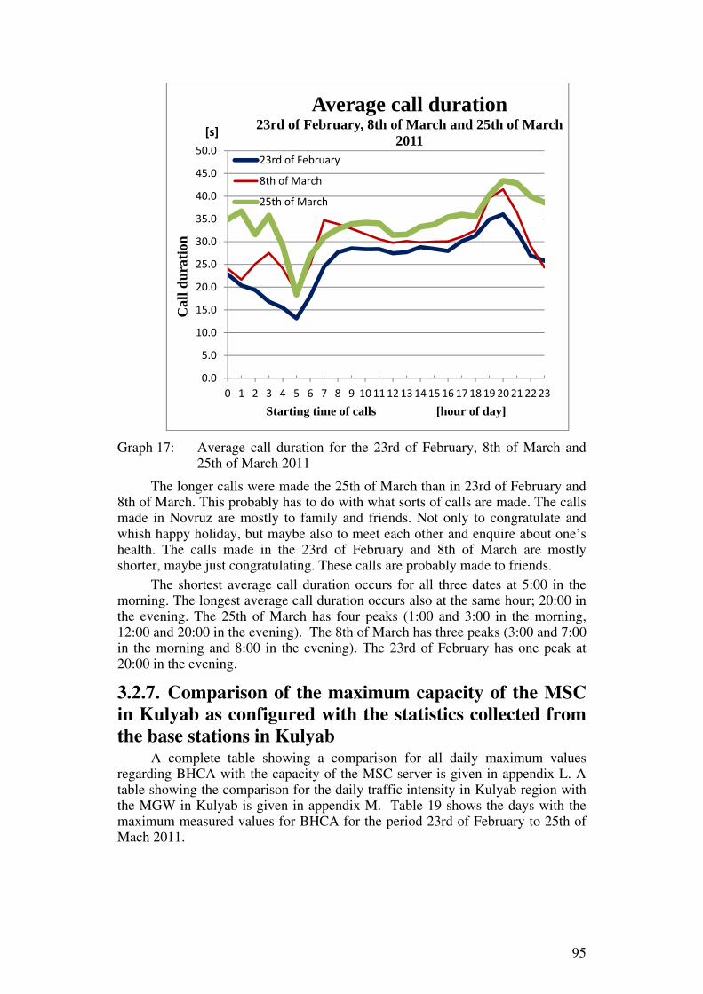
95
Graph 17: Average call duration for the 23rd of February, 8th of March and
25th of March 2011
The longer calls were made the 25th of March than in 23rd of February and 8th of March. This probably has to do with what sorts of calls are made. The calls made in Novruz are mostly to family and friends. Not only to congratulate and whish happy holiday, but maybe also to meet each other and enquire about one’s health. The calls made in the 23rd of February and 8th of March are mostly shorter, maybe just congratulating. These calls are probably made to friends.
The shortest average call duration occurs for all three dates at 5:00 in the morning. The longest average call duration occurs also at the same hour; 20:00 in the evening. The 25th of March has four peaks (1:00 and 3:00 in the morning, 12:00 and 20:00 in the evening). The 8th of March has three peaks (3:00 and 7:00 in the morning and 8:00 in the evening). The 23rd of February has one peak at 20:00 in the evening.
3.2.7. Comparison of the maximum capacity of the MSC in Kulyab as configured with the statistics collected from the base stations in Kulyab
A complete table showing a comparison for all daily maximum values regarding BHCA with the capacity of the MSC server is given in appendix L. A table showing the comparison for the daily traffic intensity in Kulyab region with the MGW in Kulyab is given in appendix M. Table 19 shows the days with the maximum measured values for BHCA for the period 23rd of February to 25th of Mach 2011.
0.0
5.0
10.0
15.0
20.0
25.0
30.0
35.0
40.0
45.0
50.0
0 1 2 3 4 5 6 7 8 9 10 11 12 13 14 15 16 17 18 19 20 21 22 23
Cal
l dur
atio
n
Starting time of calls [hour of day]
Average call duration23rd of February, 8th of March and 25th of March
201123rd of February
8th of March
25th of March
[s]

96
Table 19: Comparison of the collected BHCA statistics with the capacity of the MSC server in Kulyab
VMSC 3.033708
Collected BHCA statistics
23 of FebruaryRel. value 0.970953
% 32.005488 of March
Rel. value 0.991592% 32.68582
22 of MarchRel. value 0.866465
% 28.5612423 of March
Rel. value 0.846878
21
21
14
9
Capacity of the MSC server in Kulyab
Starting time
All the days listed in the table are national holidays. The highest measured BHCA load occurred the 8th of March. This was 32.7
% of the capacity of the MSC server used when acting as a VMSC server. Table 20 shows the comparison of the days with most traffic. The
comparison is done between the measured traffic intensity and the capacity of the MGW.

97
Table 20: Comparison of the collected traffic intensity with the capacity of the MGW in Kulyab
Capacity of the MGW in Kulyab
11.93684211 11.93684211
Collected statistics Connect traffic Respond traffic Starting time
23 of Feb.Rel. value 0.943913158 0.740142105 14
% 7.907561728 6.2004850098 of March
Rel. value 0.986015789 0.774965789 9% 8.260273369 6.492217813
19 of MarchRel. value 0.9511 0.776739474 21
% 7.967768959 6.5070767222 of March
Rel. value 0.949897368 0.763392105 21% 7.957694004 6.395260141
23 of MarchRel. value 0.964602632 0.783897368 21
% 8.080886243 6.567041446
Relative traffic load (Erlangs/Erlangs)
All days except 19th of March are national holidays. The day with the highest traffic intensity is the 8th of March as shown in Graph 1 on page 58. The connect traffic reaches in that day 8.26 % of the capacity of the MGW in Kulyab region, shown in Table 20.
It is interesting to see that the traffic load in Erlangs does not always follow the BHCA. Some days can have a high value for BHCA, but not so high value in connected traffic. The BHCA shows the intensity in the control plane and the traffic load in Erlangs shows the traffic used by the subscribers in the user plane (i.e. the actual calls).
If there are many calls with a long duration in time, then both the BHCA load and load of connected traffic have a high value. But if many shorter calls are made then the load for connect traffic is lower and the BHCA load has a high value. This has to do with that a short call and a long call have the same amount of control signaling, but different traffic load in Erlangs [10].
The 19th of March has the third highest value in terms of connect traffic load, as shown in Table 20. This day is a Saturday and is the day before the Novruz holiday begins. The BHCA value for this day reaches 26.3 % of the capacity of the MSC server, as shown in the table in appendix L.

98
3.3. Efficiency analysis for the MSC-RRP The overall traffic generated through MSC-RRP has been collected and
analyzed for the period 16th of May to the 22nd of May 2011. In the same time period has also the traffic concerning Kulyab been collected. The maximum capacity of the MSC-RRP as configured has been calculated in terms of BHCA and the traffic flow in Erlangs.
3.3.1. Calculation of the hardware capacity in MSC-RRP The calculation of the capacity for the RRP MSC server is done in the same
way as for the MSC in Kulyab. The BHCA capacity is determined by the MSC server and the traffic load in Erlangs is determined by the MGW [24].
3.3.1.1. Calculation of the BHCA capacity The MSC server RRP is also a MSOFTX3000 product from Huawei as the
MSC server in Kulyab. Thus, the calculation of the capacity of the RRP MSC server is the same as for the MSC server in Kulyab. Section 3.1.1 describes in detail how to calculate the capacity regarding BHCA.
The number of WCSU and WCCU boards determines the capacity of the MSC server [3]. The boards were counted and the capacity was calculated. A relative value for the RRP MSC server was computed relative to the BHMV (the highest measured BHCA value for the traffic in Kulyab in the period 23rd of February to the 25th of March 2011). Table 21 shows the relative values for the MSC-RRP when it acts like a VMSC.
Table 21: The capacity for the RRP MSC server in relative numbers
Name of board WCSU WCCU Maximum capacity(relative value)
x yResultTotal BHCA
VMSC 75x 75y 2.191011236Total number of links
64 Kbit/s 64x 64x2 Mbit/s 4x 4x
3.3.1.2. Calculation of the voice channel capacity for MGW-RRP The MGW RRP is also a UMG8900 product from Huawei as the MGW in
Kulyab. Thus, the calculation of the capacity of the MGW-RRP is determined in the same way as for the MGW in Kulyab. Section 3.1.2 describes in detail how to calculate the capacity regarding the traffic load.
The boards that determine the capacity of the mobile traffic are the 2SL board. Each board provide with 2*63 E1s [16]. Each E1 has 30 voice channels, one synchronization channel and one control channel [37][38]. The relative maximum capacity in MGW-RRP as configured was calculated in relation to the CHMV. The relative maximum capacity is 11.94 (Erlangs/Erlangs). The capacity for the MGW RRP is the same as for the MGW in Kulyab.
99
3.3.2. Analyzing the Kulyab traffic in the MSC-RRP When the traffic related to the Kulyab region is moved to the MSC in
Kulyab region then the remaining traffic in MSC-RRP will be able to increase using the released capacity. How much can the remaining traffic increase? That is the question that will be answered in this section.
3.3.2.1. The evaluation process All the values in the thesis are computed relative to the highest measured
value for BHCA and connected traffic. Section 2.2.1, describes in more detail about these relative values.
The capacity gain for the MSC-RRP is calculated using Equation 2. The equation requires knowing the following parameters: maximum capacity of the MSC-RRP as configured, traffic capacity generated from all base stations belonging to MSC-RRP, and traffic capacity from the base stations belonging to Kulyab region. The maximum capacity of the MSC-RRP is constant, but the traffic load changes over time. A date and an hour have to be chosen when the traffic load is high. The most interesting time is when the traffic load regarding Kulyab and the traffic load generated by all base stations in MSC-RRP are high.
Before calculating the increased capacity for the MSC-RRP, an analysis is done of the traffic situation in the MSC-RRP. This is done for the whole analyzed period and when the Kulyab traffic load is high.
3.3.2.2. Analysis for the period 16th of May to 22nd of May 2011 The available capacity in MSC-RRP will increase when the traffic load of
the Kulyab region moves to the MSC in Kulyab. This freed capacity will be both in the control plane (the parameter is BHCA) and in the user plane (the traffic load, expressed in Erlangs). All values (BHCA, traffic load for connect traffic and the percentage of the Kulyab traffic) are expressed in relative values for protection of the real values. All the BHCA values and values with the unit “call attempts” are relative to the highest measured values (BHMV) measured in the period 23rd of February to 23rd of March 2011. All the values regarding the traffic load expressed in Erlangs are relative to the highest measured value of connected traffic (CHMV) in the period 23rd of February to the 23rd of March 2011. The percentage of the Kulyab traffic in MSC-RRP are relative to the highest calculated percentage of Kulyab traffic calculated in the period 16th to 22nd of June 2011. Table 22 shows the highest measured BHCA load for Kulyab in the MSC-RRP.
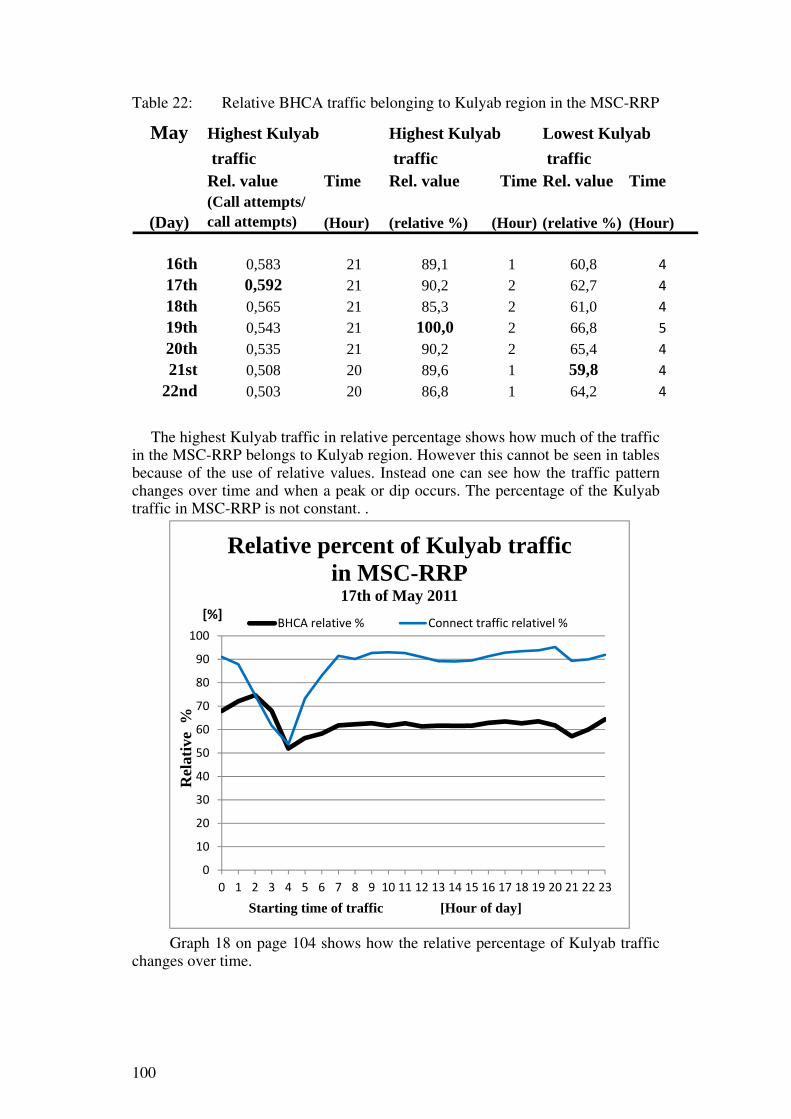
100
Table 22: Relative BHCA traffic belonging to Kulyab region in the MSC-RRP
May
Rel. value Time Rel. value Time Rel. value Time(Call attempts/call attempts)
16th 0,583 21 89,1 1 60,8 417th 0,592 21 90,2 2 62,7 418th 0,565 21 85,3 2 61,0 419th 0,543 21 100,0 2 66,8 520th 0,535 21 90,2 2 65,4 421st 0,508 20 89,6 1 59,8 4
22nd 0,503 20 86,8 1 64,2 4
(Hour)
traffic
(Day) (Hour) (relative %) (Hour) (relative %)
traffic trafficHighest Kulyab Highest Kulyab Lowest Kulyab
The highest Kulyab traffic in relative percentage shows how much of the traffic in the MSC-RRP belongs to Kulyab region. However this cannot be seen in tables because of the use of relative values. Instead one can see how the traffic pattern changes over time and when a peak or dip occurs. The percentage of the Kulyab traffic in MSC-RRP is not constant. .
Graph 18 on page 104 shows how the relative percentage of Kulyab traffic
changes over time.
0
10
20
30
40
50
60
70
80
90
100
0 1 2 3 4 5 6 7 8 9 10 11 12 13 14 15 16 17 18 19 20 21 22 23
Rel
ativ
e %
Starting time of traffic [Hour of day]
Relative percent of Kulyab traffic in MSC-RRP
17th of May 2011
BHCA relative % Connect traffic relativel %[%]
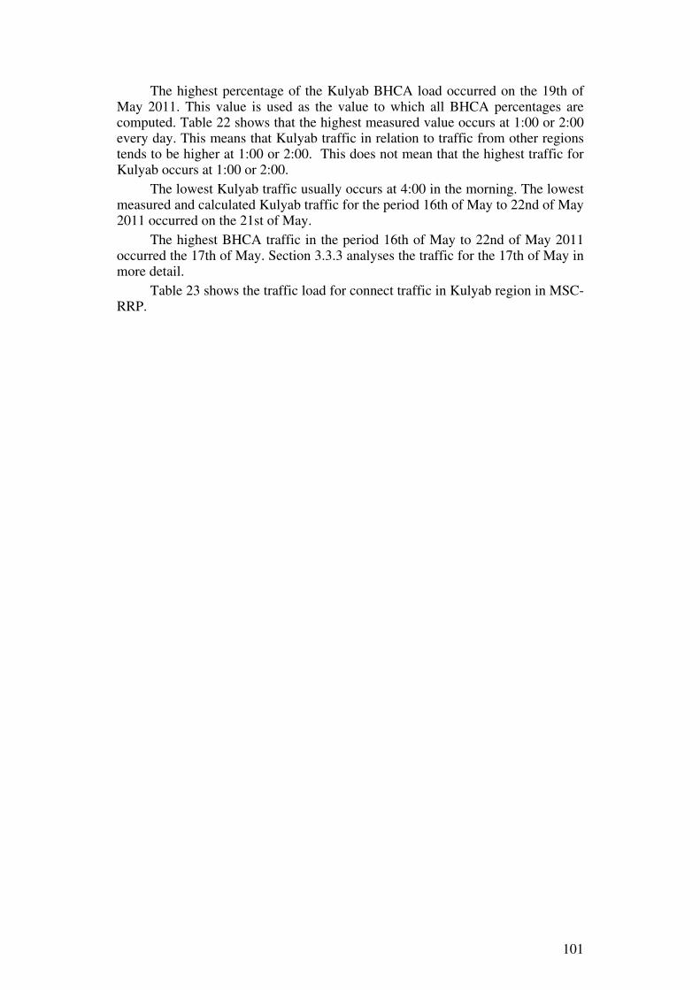
101
The highest percentage of the Kulyab BHCA load occurred on the 19th of May 2011. This value is used as the value to which all BHCA percentages are computed. Table 22 shows that the highest measured value occurs at 1:00 or 2:00 every day. This means that Kulyab traffic in relation to traffic from other regions tends to be higher at 1:00 or 2:00. This does not mean that the highest traffic for Kulyab occurs at 1:00 or 2:00.
The lowest Kulyab traffic usually occurs at 4:00 in the morning. The lowest measured and calculated Kulyab traffic for the period 16th of May to 22nd of May 2011 occurred on the 21st of May.
The highest BHCA traffic in the period 16th of May to 22nd of May 2011 occurred the 17th of May. Section 3.3.3 analyses the traffic for the 17th of May in more detail.
Table 23 shows the traffic load for connect traffic in Kulyab region in MSC-RRP.

102
Table 23: Connect traffic belonging to Kulyab in the MSC-RRP
May
rel. value Time rel. value Time rel. value Time(Day) (Erlangs/ (Hour) (rel. %) (Hour) (rel. %) (Hour)
Erlangs)
16th 0.947 21 95.4 9 49.2 417th 0.967 21 95.2 20 53.7 418th 0.935 21 95.8 1 55.2 419th 0.925 21 100.0 1 57.4 420th 0.923 21 93.8 23 59.0 421st 0.816 21 94.3 23 56.5 422nd 0.855 21 94.6 0 57.0 4
Highest Kulyab Highest Kulyab Lowest Kulyab traffic traffic traffic
The highest calculated percentage of connect traffic for Kulyab region in
relation to other regions in MSC-RRP occurred on the 19th of May 2011, as shown in Table 23. The same day and the same hour as for the BHCA traffic load. The lowest percentage of connect traffic for Kulyab region in relation to other regions in MSC-RRP occurred at 4:00 in the morning, as shown in Table 23. Table 22 shows that this also occurred for BHCA traffic. Meaning that, in relation to traffic from other regions, the people in Kulyab do not make so many calls at 4:00 in the morning. The highest percentage of connect traffic for Kulyab region in relation to traffic from other regions in MSC-RRP occurred late (with the exception of the 16th of May), as shown in Table 23.
The highest traffic load for Kulyab region occurred the 17th of May at 21:00. Section 3.3.3 analyses in more detail the traffic situation for that day.
Table 24 shows the relative percentage of Kulyab traffic when there is high intensity in traffic.

103
Table 24: Relative percentage of Kulyab traffic when there is a peak in the Kulyab traffic load
May Relative Relativepercentage percentage
Rel. value Time Rel. value Time (Call attempts/ (Erlangs/ call attempts) Erlangs)
16th 0.583 21 67.8 0.947 21 87.917th 0.592 21 69.0 0.967 21 89.318th 0.565 21 71.5 0.935 21 91.619th 0.543 21 70.5 0.925 21 91.420th 0.535 21 67.1 0.923 21 88.421st 0.508 20 72.8 0.816 21 85.0
22nd 0.503 20 73.4 0.855 21 92.1
Kylyab trafficBHCA Connect trafficHighest traffic Highest traffic
(Day) (Hour) (rel. %) (Hour) (rel. %)
The values in bold are interesting values to examine in more detail. Table 24 shows that on the 17th of May at 21:00 there is a peak in traffic for Kulyab region (both regarding to BHCA and connected traffic load), but the relative percentage for Kulyab region is not at its highest value.
The highest percentage of Kulyab traffic in regard to high traffic intensity for BHCA traffic load occurs the 22nd of May 2011 at 20:00 with regard to when there is a peak in Kulyab traffic. The 18th of May at 21:00 is when there is a peak in BHCA traffic for the total of MSC-RRP. In this day and hour there also is a peak for the percentage of Kulyab traffic with regard to connected traffic load. This involves both the highest traffic load for the total of MSC-RRP and for Kulyab traffic. These days and hours are worth calculating the capacity gain for the MSC-RRP.
3.3.3. Analysis of the traffic on the 17th of May 2011 The values for each hour are given in appendix N. Table 25 shows a part of
this list. The highest traffic in Kulyab region occurred at 21:00 for both BHCA and connected traffic load. The relative percentage was not at its highest peak then.
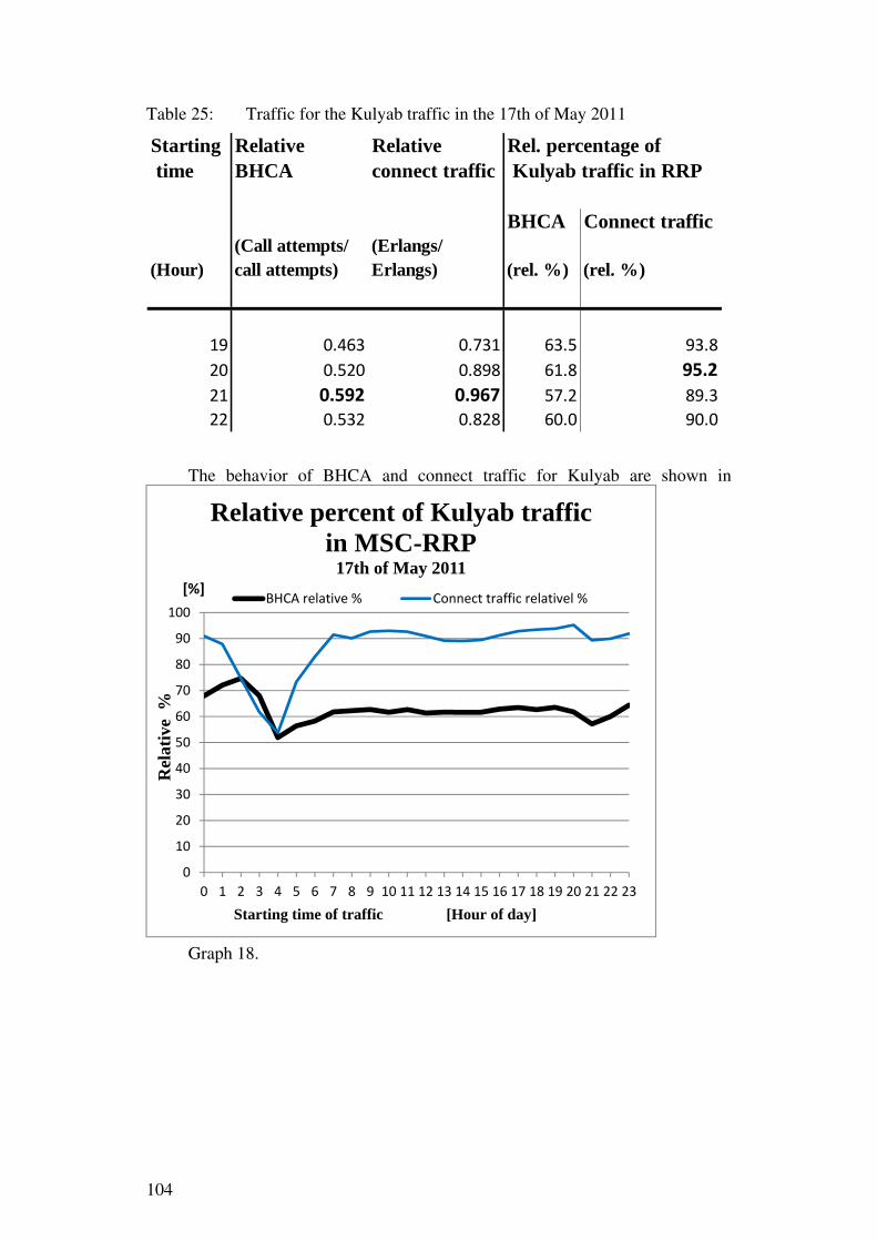
104
Table 25: Traffic for the Kulyab traffic in the 17th of May 2011
Starting Relative Relative time BHCA connect traffic
BHCA Connect traffic(Call attempts/ (Erlangs/call attempts) Erlangs)
19 0.463 0.731 63.5 93.820 0.520 0.898 61.8 95.221 0.592 0.967 57.2 89.322 0.532 0.828 60.0 90.0
Rel. percentage of Kulyab traffic in RRP
(Hour) (rel. %) (rel. %)
The behavior of BHCA and connect traffic for Kulyab are shown in
Graph 18.
0
10
20
30
40
50
60
70
80
90
100
0 1 2 3 4 5 6 7 8 9 10 11 12 13 14 15 16 17 18 19 20 21 22 23
Rel
ativ
e %
Starting time of traffic [Hour of day]
Relative percent of Kulyab traffic in MSC-RRP
17th of May 2011
BHCA relative % Connect traffic relativel %[%]

105
Graph 18: Relative percentage of Kulyab traffic in MSC-RRP for the 17th of
May
The percentage of BHCA and connect traffic load for Kulyab region in relation to the other regions in MSC-RRP are shown in the graph above,
0
10
20
30
40
50
60
70
80
90
100
0 1 2 3 4 5 6 7 8 9 10 11 12 13 14 15 16 17 18 19 20 21 22 23
Rel
ativ
e %
Starting time of traffic [Hour of day]
Relative percent of Kulyab traffic in MSC-RRP
17th of May 2011
BHCA relative % Connect traffic relativel %[%]
0
10
20
30
40
50
60
70
80
90
100
0 1 2 3 4 5 6 7 8 9 10 11 12 13 14 15 16 17 18 19 20 21 22 23
Rel
ativ
e %
Starting time of traffic [Hour of day]
Relative percent of Kulyab traffic in MSC-RRP
17th of May 2011
BHCA relative % Connect traffic relativel %[%]

106
Graph 18. Note that the values are relative. The highest percentage for BHCA and connected traffic were measured on the 19th of May 2011 for both BHCA and connect traffic. They are used as the value to which all other values relate to. This means that the values do not show how much of the traffic in MSC-RRP belongs to Kulyab region. The values show only how the traffic changes over time and when it has a peak or a dip.
Graph 18 shows that at 2:00 in the morning there is a peak in BHCA traffic
load. This means that compared to other regions in MSC-RRP, the people in Kulyab region tend to call more frequently at 2:00 in the morning,
3.3.3.1. Calculation of the potential capacity gain for MSC-RRP The increased capacities are calculated regarding BHCA and connected
traffic load by using Equation 2. Appendix O explains in more detail how the formula was derived.
The day and time when a peak in traffic occurs is chosen. Table 24 gives the relative percentage of Kulyab traffic when there was a peak in Kulyab traffic.
There was a peak in traffic for Kulyab region on the 17th of May 2011 at 21:00. The peak occurred both for BHCA and connected traffic. The peak for the traffic load regarding all regions in MSC-RRP occurred on the 16th of May 2011 at 21:00.
The day and time when there was a peak in the percentage of Kulyab traffic was chosen both regarding when there was a peak in Kulyab traffic (22nd of May at 20:00) and when there was a peak in the total traffic for the MSC-RRP (18th of May at 21:00). Also the day and time when there was a fall in the percentage of Kulyab traffic when there was high intensity traffic was chosen. This occurred the 21st of May at 21:00 regarding BHCA and connected traffic load.
0
10
20
30
40
50
60
70
80
90
100
0 1 2 3 4 5 6 7 8 9 10 11 12 13 14 15 16 17 18 19 20 21 22 23
Rel
ativ
e %
Starting time of traffic [Hour of day]
Relative percent of Kulyab traffic in MSC-RRP
17th of May 2011
BHCA relative % Connect traffic relativel %[%]
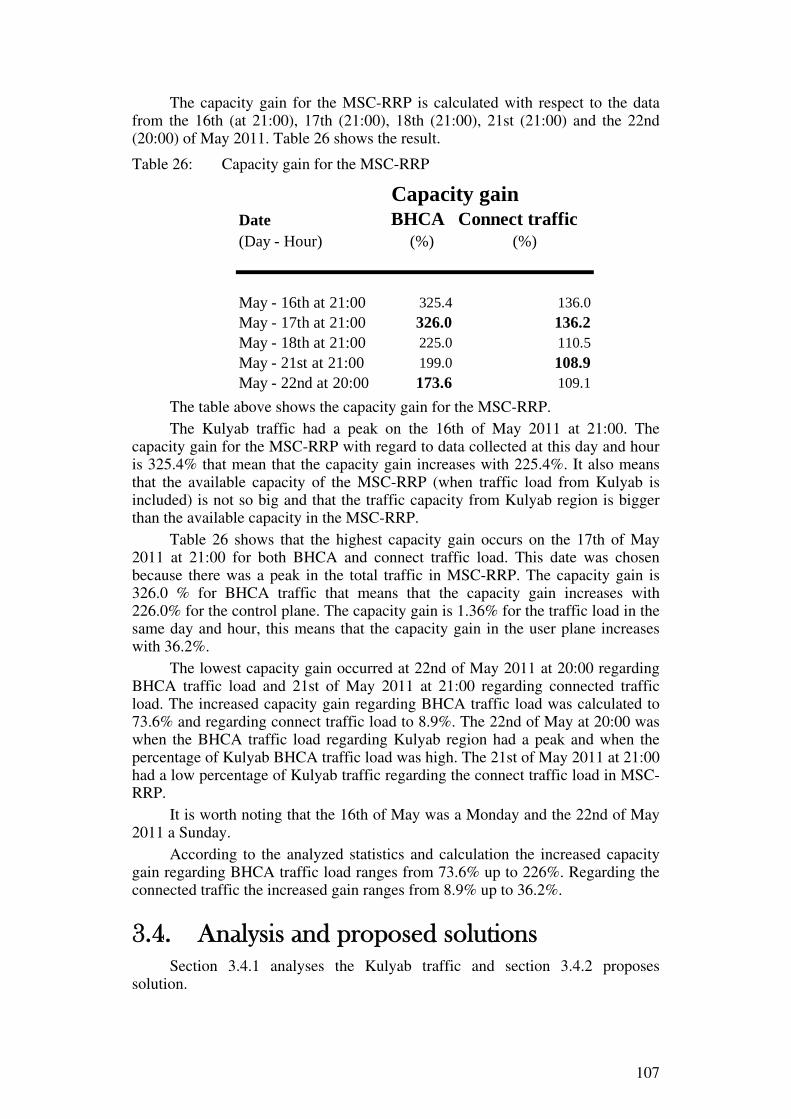
107
The capacity gain for the MSC-RRP is calculated with respect to the data from the 16th (at 21:00), 17th (21:00), 18th (21:00), 21st (21:00) and the 22nd (20:00) of May 2011. Table 26 shows the result.
Table 26: Capacity gain for the MSC-RRP
Date BHCA Connect traffic(Day - Hour) (%) (%)
May - 16th at 21:00 325.4 136.0May - 17th at 21:00 326.0 136.2May - 18th at 21:00 225.0 110.5May - 21st at 21:00 199.0 108.9May - 22nd at 20:00 173.6 109.1
Capacity gain
The table above shows the capacity gain for the MSC-RRP. The Kulyab traffic had a peak on the 16th of May 2011 at 21:00. The
capacity gain for the MSC-RRP with regard to data collected at this day and hour is 325.4% that mean that the capacity gain increases with 225.4%. It also means that the available capacity of the MSC-RRP (when traffic load from Kulyab is included) is not so big and that the traffic capacity from Kulyab region is bigger than the available capacity in the MSC-RRP.
Table 26 shows that the highest capacity gain occurs on the 17th of May 2011 at 21:00 for both BHCA and connect traffic load. This date was chosen because there was a peak in the total traffic in MSC-RRP. The capacity gain is 326.0 % for BHCA traffic that means that the capacity gain increases with 226.0% for the control plane. The capacity gain is 1.36% for the traffic load in the same day and hour, this means that the capacity gain in the user plane increases with 36.2%.
The lowest capacity gain occurred at 22nd of May 2011 at 20:00 regarding BHCA traffic load and 21st of May 2011 at 21:00 regarding connected traffic load. The increased capacity gain regarding BHCA traffic load was calculated to 73.6% and regarding connect traffic load to 8.9%. The 22nd of May at 20:00 was when the BHCA traffic load regarding Kulyab region had a peak and when the percentage of Kulyab BHCA traffic load was high. The 21st of May 2011 at 21:00 had a low percentage of Kulyab traffic regarding the connect traffic load in MSC-RRP.
It is worth noting that the 16th of May was a Monday and the 22nd of May 2011 a Sunday.
According to the analyzed statistics and calculation the increased capacity gain regarding BHCA traffic load ranges from 73.6% up to 226%. Regarding the connected traffic the increased gain ranges from 8.9% up to 36.2%.
3.4. Analysis and proposed solutions Section 3.4.1 analyses the Kulyab traffic and section 3.4.2 proposes
solution.
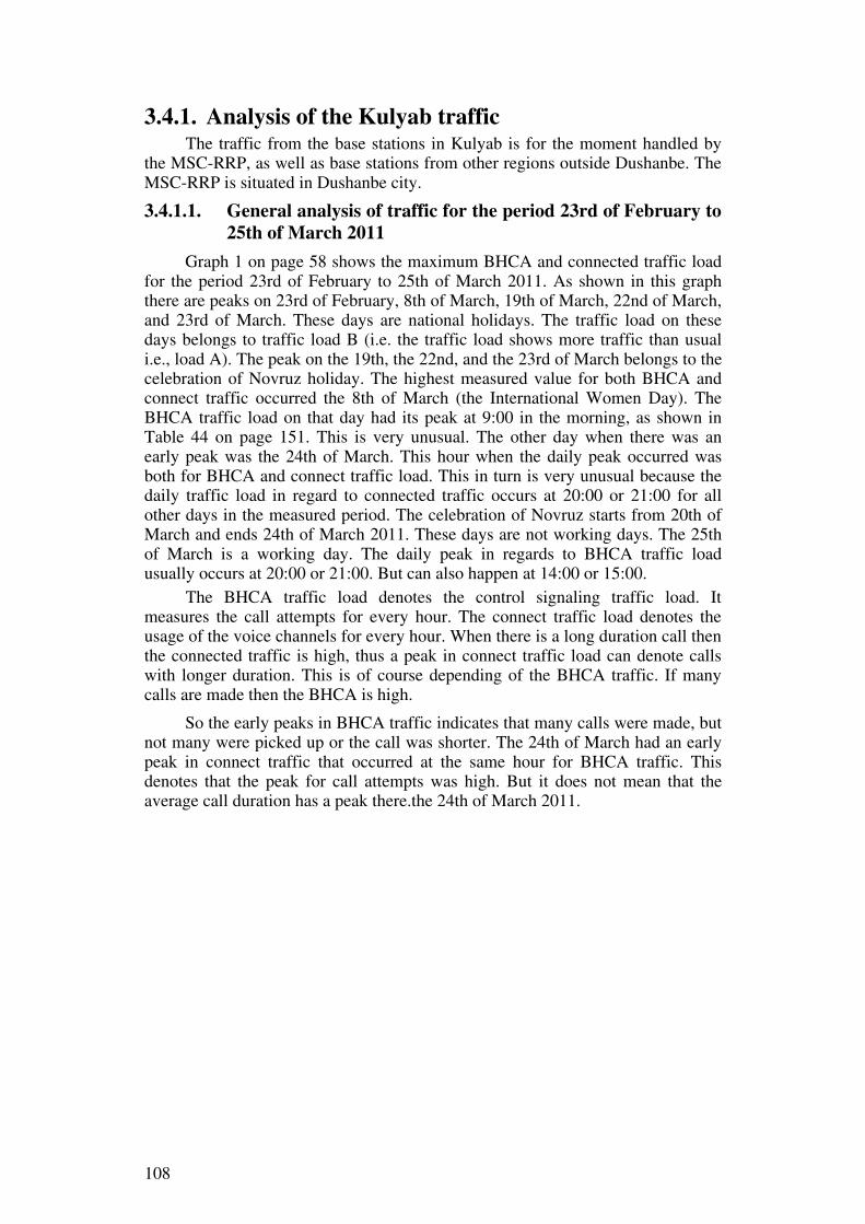
108
3.4.1. Analysis of the Kulyab traffic The traffic from the base stations in Kulyab is for the moment handled by
the MSC-RRP, as well as base stations from other regions outside Dushanbe. The MSC-RRP is situated in Dushanbe city.
3.4.1.1. General analysis of traffic for the period 23rd of February to 25th of March 2011
Graph 1 on page 58 shows the maximum BHCA and connected traffic load for the period 23rd of February to 25th of March 2011. As shown in this graph there are peaks on 23rd of February, 8th of March, 19th of March, 22nd of March, and 23rd of March. These days are national holidays. The traffic load on these days belongs to traffic load B (i.e. the traffic load shows more traffic than usual i.e., load A). The peak on the 19th, the 22nd, and the 23rd of March belongs to the celebration of Novruz holiday. The highest measured value for both BHCA and connect traffic occurred the 8th of March (the International Women Day). The BHCA traffic load on that day had its peak at 9:00 in the morning, as shown in Table 44 on page 151. This is very unusual. The other day when there was an early peak was the 24th of March. This hour when the daily peak occurred was both for BHCA and connect traffic load. This in turn is very unusual because the daily traffic load in regard to connected traffic occurs at 20:00 or 21:00 for all other days in the measured period. The celebration of Novruz starts from 20th of March and ends 24th of March 2011. These days are not working days. The 25th of March is a working day. The daily peak in regards to BHCA traffic load usually occurs at 20:00 or 21:00. But can also happen at 14:00 or 15:00.
The BHCA traffic load denotes the control signaling traffic load. It measures the call attempts for every hour. The connect traffic load denotes the usage of the voice channels for every hour. When there is a long duration call then the connected traffic is high, thus a peak in connect traffic load can denote calls with longer duration. This is of course depending of the BHCA traffic. If many calls are made then the BHCA is high.
So the early peaks in BHCA traffic indicates that many calls were made, but not many were picked up or the call was shorter. The 24th of March had an early peak in connect traffic that occurred at the same hour for BHCA traffic. This denotes that the peak for call attempts was high. But it does not mean that the average call duration has a peak there.the 24th of March 2011.
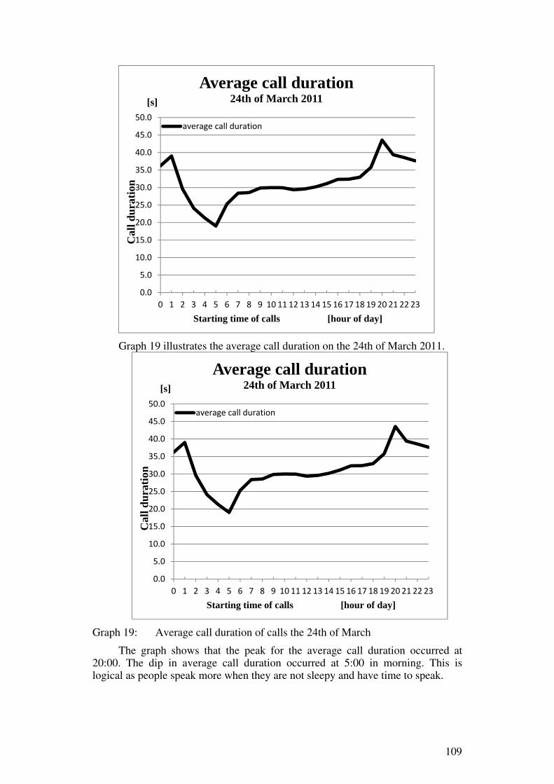
109
Graph 19 illustrates the average call duration on the 24th of March 2011.
Graph 19: Average call duration of calls the 24th of March
The graph shows that the peak for the average call duration occurred at 20:00. The dip in average call duration occurred at 5:00 in morning. This is logical as people speak more when they are not sleepy and have time to speak.
0.0
5.0
10.0
15.0
20.0
25.0
30.0
35.0
40.0
45.0
50.0
0 1 2 3 4 5 6 7 8 9 10 11 12 13 14 15 16 17 18 19 20 21 22 23
Cal
l dur
atio
n
Starting time of calls [hour of day]
Average call duration24th of March 2011
average call duration
[s]
0.0
5.0
10.0
15.0
20.0
25.0
30.0
35.0
40.0
45.0
50.0
0 1 2 3 4 5 6 7 8 9 10 11 12 13 14 15 16 17 18 19 20 21 22 23
Cal
l dur
atio
n
Starting time of calls [hour of day]
Average call duration24th of March 2011
average call duration
[s]

110
3.4.1.2. Analysis of the Kulyab traffic in comparison to the maximum capacity of the MSC in Kulyab as configured
Table 45 on page 153 shows the percentage of BHCA traffic in the MSC server in Kulyab and Table 46 on page 157 shows the percentage of relative connected traffic load in the MGW in Kulyab.
The highest measured value both for BHCA and connect traffic load occurred On the 8th of March 2011. The usage of the MSC server was at that time 32.7% and for the MGW 8.26%, as shown in Table 45 and Table 46.
The MSC in Kulyab has thus a much higher capacity than the traffic generated in Kulyab.
3.4.1.3. Analysis of the Kulyab traffic in the MSC-RRP The statistics for the Kulyab traffic in the MSC-RRP were collected from
the 16th of May to the 22nd of May 2011. The capacity gain for the MSC-RRP was calculated using Equation 2. Appendix O shows how the equation was derived. Table 26 on page 107 shows the capacity gain for some chosen days and hours.
The capacity gain regarding BHCA traffic ranges from an increase of 73.6% up to 226.0%. The capacity gain regarding connect traffic load ranges from 8.95% up to 36.2%. Both the capacity gain regarding BHCA and connect traffic load show a big range in percentage.
The statistics were only collected for a week. The variation in traffic can differ for a lot of reasons. The difference in traffic can depend on the day of week. If the statistics were collected for more than one week, one could learn if the difference was due to the day of week. The statistics should be collected for at least three weeks for a better analysis. According to the statistics the capacity gain for the MSC-RRP will be at least 73.6% regarding BHCA traffic and 8.95% regarding connect traffic load. This means that the control signaling (BHCA traffic) can increase with 73.6% and still have a good throughput and the connect traffic load can increase with 8.95%.
3.4.1.4. Analysis of the traffic situation with a MSC in Kulyab region The traffic in Kulyab region will improve with a MSC situated in Kulyab
region. Currently the MSC-RRP takes care of all 2G traffic generated from regions outside Dushanbe city. This includes the traffic generated by the base stations situated in Kulyab. This means that the traffic from the Kulyab base stations have to transverse optical links to Dushanbe where the MSC-RRP is situated. This creates unnecessary traffic and unnecessary usage of the optical links. If a call is within the Kulyab region, then the control signaling and voice bearer have to be connected through the MSC-RRP to the base stations situated in Kulyab. This usage of the optical links will not be needed when there is a MSC in Kulyab region as the traffic in Kulyab will be local. The traffic between the base stations in Kulyab and the MSC in Kulyab will transverse a shorter distance. A call within Kulyab region does not need to traverse to the MSC-RRP situated in Dushanbe city. This will increase throughput as well as reliability.
The call drop rate will be lower with a MSC in Kulyab region. This will occur both for calls within the Kulyab region as well as for calls with a caller or callee in Kulyab region. This will occur because the control signaling and voice bearer does not need to traverse such a long distance hence the handover success rate for handover between cells and base stations in Kulyab area will increase due to decrease in delay.

111
With MSCs responsible for each region, then only the traffic for that region is relevant. Different regions may have different requirements and different demands. Some areas may require calls with longer duration (thus the capacity for the connected and response traffic has to be higher), other areas maybe require greater capacity for making many short calls (thus the capacity on terms of BHCA has to be higher) and other regions might require higher data speed (requirement of GPRS). To configure MSCs that suits the traffic requirement for a specific area improves the usability.
When there will be a MSC in Kulyab then the traffic capacity regarding Kulyab region will move to the MSC in Kulyab and free more capacity in the MSC-RRP. Thus the MSC-RRP will gain more capacity and the remaining traffic can grow in the control plane as well as in the user plane.
3.4.2. Proposed solution The capacity of the MSC in Kulyab has much greater capacity than
required. It can easily support the base stations in LAC 0050 and 0051. The highest traffic in the period 23rd of March 2011 to 25th of March 2011 was measured the 8th of March. It is a national holiday and thus counts as a load B. The peak at that day occurred at 9:00 in the morning for BHCA traffic and 21:00 for connected traffic load. The usage of the MSC server was 32.7% regarding BHCA traffic and 8.3% regarding connected traffic load. This means that the MSC in Kulyab can handle load B situations very well. The MSC in Kulyab has a much greater capacity then is now needed in Kulyab region.
The MSC in Kulyab is already bought and equipped with the hardware. Perhaps the MSC can handle even load C traffic situations. This load is impossible to calculate because the amount of traffic is unknown; also one does not know when it will happen. Earthquakes can happen; therefore an overcapacity in the MSC in Kulyab is good to have.
A MSC with local traffic (i.e. the base stations are relative near to the MSC) has good reliability. The signaling and voice channels do not have to traverse unnecessary distances. Longer distances increase probability of failure. Thus shorter distances have better reliability.
The aim of the thesis project was to analyze the traffic regarding Kulyab region. The analysis can be done in several ways. The thesis project has focused on analyzing the traffic regarding BHCA and connect traffic load. Some analysis has also been done with regard to response times and response traffic load for calculating the average call duration. Other interesting parameters worth analyzing are call drop rate and call success rate. However, these have not been analyzed because the aim of the thesis is to analyze Kulyab traffic in order to configure a MSC in Kulyab region. The first question is if the MSC in Kulyab can handle the traffic in the region. The thesis has shown that the MSC in Kulyab can very easily responsibility for the base stations in Kulyab. It even can handle traffic load B, and maybe even traffic load C.
Another interesting question is how well the MSC in Kulyab can handle the traffic in Kulyab. To be able to answer this question the MSC has to be configured and installed in Kulyab region, than it will be possible to analyze the call drop rate and handover success and compare it to when the base stations belonged to MSC-RRP.

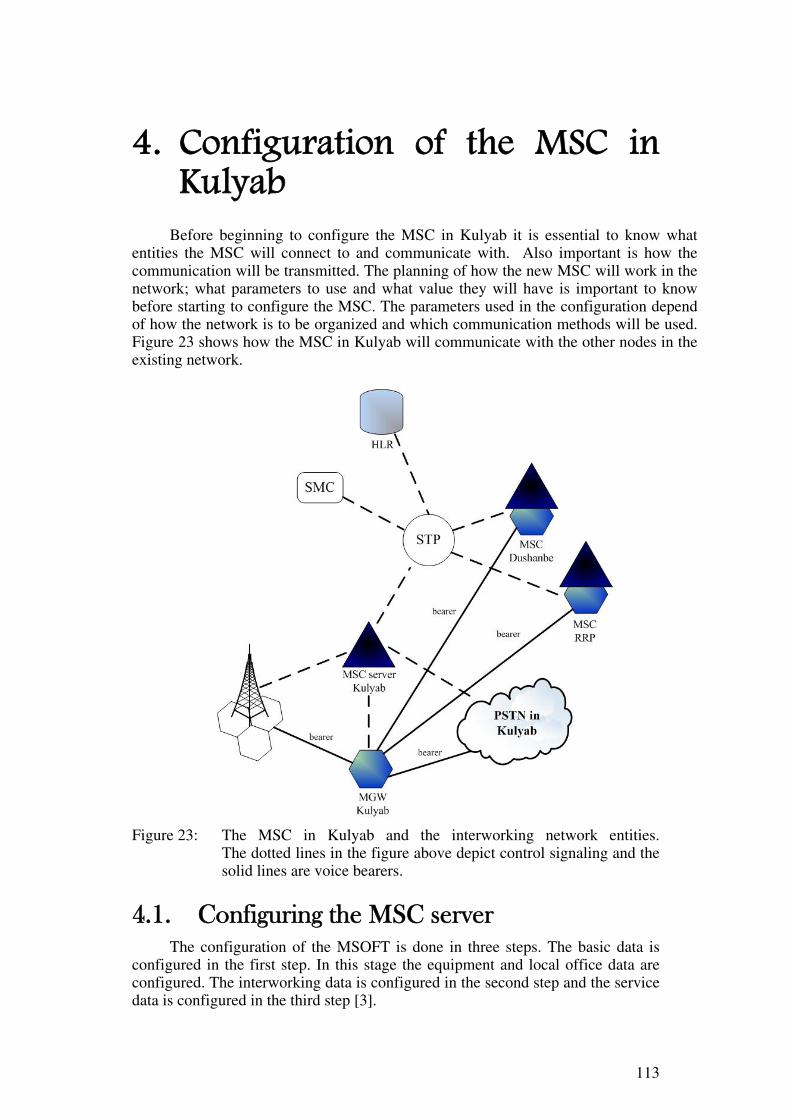
113
4. Configuration of the MSC in Kulyab
Before beginning to configure the MSC in Kulyab it is essential to know what
entities the MSC will connect to and communicate with. Also important is how the communication will be transmitted. The planning of how the new MSC will work in the network; what parameters to use and what value they will have is important to know before starting to configure the MSC. The parameters used in the configuration depend of how the network is to be organized and which communication methods will be used. Figure 23 shows how the MSC in Kulyab will communicate with the other nodes in the existing network.
Figure 23: The MSC in Kulyab and the interworking network entities. The dotted lines in the figure above depict control signaling and the solid lines are voice bearers.
4.1. Configuring the MSC server The configuration of the MSOFT is done in three steps. The basic data is
configured in the first step. In this stage the equipment and local office data are configured. The interworking data is configured in the second step and the service data is configured in the third step [3].

114
4.1.1. Step 1: Configuration of the basic data The configuration of the basic data is done in two steps. First the equipment
data is configured and after that the data of the local office is configured [3].
4.1.1.1. Configuration of the equipment data The shelves, frames, and boards used by the MSOFT must be identified. If
they are not identified, then the MSOFT will not be able to recognize the boards and use them.
The structure of the MSOFTX is composed of cabinets called shelves. Each shelf is composed of frames. One of the frames is the controlling frame of the MSOFT and called the basic subrack. The other frames are called expansion subracks. Each frame has 21 slots where boards can be inserted. Boards can be inserted at both the front and at the back of a frame [3].
Boards that distribute messages internally in the MSOFT have a module number enabling them to be identified by the MSOFT. The boards that work as a pair in 1+1 backup mode share the same module number and the boards that work in load sharing mode each have a unique module number. Every module number is unique. The boards situated in the back, the alarm board, and power supply boards have no module number [3].
A configuration example is shown in appendix Q.
4.1.1.2. Configuration of local office data The configuration of the local office data enables the MSC server to
communicate with other network elements. It identifies the MSC server in the mobile network, so other network elements can find and communicate with MSC.
Important data that belongs to the scope of local office data are the MSRN, HON allocation, and data about the Mc interface. The HON (handover number) is allocated by the MSC to the MS when the MS is roaming and enters an area covered by another MSC (potentially leading to inter-MSC handover).
Some of the properties that a MSC server can have are: office type, signaling point code, MSC and VLR number, and signaling network. The office type tells what kind of SS7 network identifier the MSC server belongs to. There are four types of SS7 network identifiers: international identifier, international reserved network, national network, and national reserved network. The MSC server in Kulyab will be part of a national network and a national reserved network. The signaling point code uniquely identifies a node in the signaling network. The MSC number and VLR number are the same, because the VLR belongs to and is situated in a MSC server. The coding format for the MSC and VLR number is an E.164 string with the format: CC (country code) +NDC (national destination code) +LSP (locally significant part) [3].
Appendix R shows an example of the local office configuration.
4.1.2. Step 2: Configuring the interworking data The MSC server interworks with several network entities. To enable the
communication between the MSC server and the network entities that interwork with the MSC server, the information about the connection between the MSC server and each of the network entities have to be configured [3].

115
One of these important network entities is the MGW. The MGW provides the actual subscriber service, such as switching voice traffic. The connection with MGW is done using IP, TDM or IP, and TDM. The messages that are exchanged between the MSC server and the MGW use the H.248 protocol.
Another important network entity is the BSC. The BSC is responsible for controlling the base stations (mentioned earlier) and interworks with the MSC server and the MGW [3]. Without the BSC there is no communication with the base stations and hence no calls can be made or received. The connection between the MSC server and the BSC can be configured in five different ways depending upon the connection between them. It can be MTP based, M2UA based, M3UA based, Mini-A flex based, or IP-based A-interface model [3].
Another important network entity to interwork with is with the HLR. The HLR is a database that stores information about the subscribers that belong to the mobile network. The connection with the HLR can be via five different protocols: MTP, M2UA, M3UA non-peer-to-peer, M3UA peer-to-peer, and as STP [3].
To be able to connect calls and perform handovers for a MS not belonging to the current MSC, the MSC has to be able to communicate with other MSCs. That is done through the MC interface. The configuration of the MC-interface can utilize the following protocols: ISUP over MTP, ISUP over M3UA, BICC over M3UA, and SIP-I [3].
Because the MSC server in Kulyab will act as a 2G VMSC, the communication between the MSC server and a SMS center (SMC) must be configured. The MSC server in Kulyab uses the M3UA protocol when communicating with the SMC. To communicate with the SPC, the MSC server in Kulyab uses STP network mode.
4.1.3. Step 3: Configuring basic service data After configuring the basic data and the interworking data the basic service
data is configured. The MSC server in Kulyab will act as a VMSC. Table 27 shows the different tasks that a VMSC has to perform [3].
Table 27: Tasks managed by a VMSC [3]
Basic number analysis Manage BSC Control authentication Roaming management Manage LAI and GCI Control paging
116
4.2. Configuring the MGW The configuration of the MGW is done in six steps. In the first step the basic
data is configured. In this step the frames, the board, the clock, and the physical interface are configured. The second step involves configuring of the control data of the MGW. The H.248 links and the MGW data are configured in this step. The third step involves configuration of the bearer that the MGW will support. The bearer is the actual channel where the voice is carried. The UMG supports TDM bearer for the access side; and TDM bearer and IP bearer for the core network side. The forth step involves the configuration of the signaling transfer point. The signaling transfer point will interact between the media gateway and the PSTN and between the media gateway and MSC. The signaling between these network entities can be done using SIGTRAN over MTP2 or M3Ua, semi-permanent connection, or channel associated signaling (CAS). The fifth step in the configuration of the UMG involves the configuration of the CODEC capability set. CODEC can be used to enhance the voice quality. The sixth strep involves the configuration of the MSC pool data. This step is optional and is only used when a MGW connects to more than one MSC server [16].
117
5. Conclusions and Future Work Conclusions of the thesis work are given in Section 5.1. Section 5.2
discusses the future work that might be done other then the configuration and installation of the MSC.
5.1. Conclusions The goal of this thesis project was achieved. I analyzed the Kulyab traffic
and determined that the MSC in Kulyab region can handle the base stations in Kulyab region. Table 45 on page 153 and Table 46 on page 157 show the relative usage (and percentage utilization) of the MSC in Kulyab. The collected statistics for the period 23rd of February to 25th of March 2011 show that the MSC in Kulyab can very easily handle load B traffic and maybe even load C traffic.
When analyzing the Kulyab traffic it was observed that the daily maximum peak occurred at 20:00 or 21:00 for connected traffic with the exception of the 24th of March when the peak occurred at 9:00 in the morning. The daily peak in BHCA traffic had its daily peak mostly at 20:00 or 21:00, but could also have a daily peak at 14:00 or 15:00. Only for two days were daily peaks at 9:00 for BHCA. Both of these days were not normal working days. One of those days was the 8th of March (International Women’s Day) and the other day was the 24th of March (the last day of the Novruz celebration).
The peaks observed for the whole period 23rd of February to 25th of March 2011 were observed on national holidays (load B traffic). Graph 1 on page 58 shows the peaks for the whole measured period regarding both BHCA and connect traffic load. It is interesting to see how very well the traffic pattern follows a pattern. The traffic shows the behavior of the users both in their daily usage and over a long time period.
The peaks were observed on national holidays (load B traffic) when observing the traffic over a long period of time. The daily peaks regarding connect traffic load were observed at 20:00 or 21:00 with the exception of 24th of May 2011. This means that the duration of all call attempts that were successful connected had its highest value at that time. In this time work is finished and people have had their dinners, so there is time for speaking with friends and relatives. The traffic load in terms of both BHCA and connect traffic load decreases after 20:00 and 21:00.
The BHCA load denotes call attempts, meaning that when there was a peak in BHCA then there were made a lot of call attempts. When there was a peak in BHCA at 14:00 or 15:00 and the peak on connected traffic load at 20:00 or 21:00, this indicates there was a call attempt but the callee did not pick up or the call duration was very short. This is very likely to happen during working days when people are at work and cannot speak for a long time.
It should not come as a surprise that the mobile traffic follows the behavior of the users, but it is very interesting to observe it in detail. The need to communicate is very human and very important. By observing the needs of the subscribers in an area one can tailor a service for these subscribers.

118
The usage of the network is not even, there are peaks and valleys. This occurs during the course of a day, as well as during long periods of time. One can predict when load B will occur because there is a holiday (a day of celebrations), but load C traffic is unpredictable. Because the network usage is not so high late at night and early in the mornings, paging of MSs does not need to be so frequent. The capacity of the base station does not need to be so high during these hours. It would be good to have a capacity that depends on the usage. When usage is high more capacity is needed and when usage is low less capacity is needed. Hence one might use less capacity when there is low usage to save electricity.
The technology regarding mobile networks is in constant development. It is important to try to keep up with the technology as well as the demands of the subscribers. Analysis of the subscribers’ needs and demands are essential. The network has to be able to handle the load generated by their subscribers, but the quality of service is also very important. The quality of service involves the call quality, call success rates and the availability of other services such as email and downloading data.
The choice of which new technology to implement is not easy. Some new technologies may seem to be very good initially, but after two years can be surpassed by another totally different technology. This means that when it is necessary to buy new equipment it is important to observe the subscribers’ needs at that time and to predict traffic for three or four years in advance. Trying to predict the users’ needs in the distant future is not recommended. The technology changes rapidly as do the needs and demands of the subscribers. Trying to implement a new technology that currently is not in demand and may not be in demand for the next year can be bad economically.
Reusing old equipment is good when supporting the traffic of subscribers if their demands are not high. The 2G technology is already an old technology, but it still works well for call services, hence an operator can still have a good business supporting their subscribers using old equipment.
Before the subscribers demand new services one should predict this demand and install the necessary new equipment in advance of the demand. This can be done by observing what kind of cell phones are in the market and analyzing the traffic of the subscribers.
5.2. Future work The analysis of the Kulyab traffic regarding usage capacity is done. The
next thing to do is to configure and install the MSC in Kulyab. After configuring and installing the MSC in Kulyab one can measure how well it actually performs. It is essential to collect information about the Kulyab traffic from the MSC-RRP in advance so that the performance of the MSC in Kulyab can be compared to when the MSC-RRP handled the base stations in the Kulyab region.
When collecting statistics it is important to plan what you want to analyze and what you will need in order for the work to be done. Planning is essential. With a good planning there are few mistakes. Be sure that the statistics you have collected are what you need. If you need more statistics collect all of them during the same period of time.

119
Do not wait a long time between collecting data and using this data for statistical analysis. When you use the statistics you may discover that some data is missing and you might be able to retrieve the missing data. The statistics in the BAM are available only for one week, hence information not retrieved after one week is gone.


121
References [1] Tom Tullis and Bill Albert. Measuring the User Experience: Collecting,
Analyzing, and Presenting Usability Metrics. Morgan Kaufmann Publishers. 2008, ISBN:978-0-12-373558-4.
[2] Yi-Bing Lin and Imrich Chlamtac, Wireless and Mobile Network Architectures. John Wiley & Sons, 2001, ISBN: 978-0-471-39492-1.
[3] Huawei Technologies Co., Ltd., MSOFTX3000 Product Documentation. V100R008C02. Huawei. version 6. 30 June 2010
[4] Andy Valdar. Understanding Telecommunications Networks. Institution of Engineering and Technology, London, United Kingdom. 2006. ISBN: 978-086341-362-9
[5] Ajay R. Mishra (editor). Advanced Cellular Network Planning and Optimisation: 2G/2.5G/3G...Evolution to 4G. John Wiley & Sons. 2007. ISBN: 978-0-470-01471-4
[6] Peter Stuckmann. The GSM Evolution: Mobile Packet Data Services, Chapter 2: Packet Data Support in GSM Networks. John Wiley & Sons. 2003. ISBN: 978-0-470-84855-3
[7] Sumit Kasera and Nishit Narang. 3G networks: architecture. protocols and procedures: based on 3GPP specifications for UMTS WCDMA networks. 2004. Tata McGraw-Hill Publishing Company Limited. ISBN:978-0-07-052799-7
[8] Mark Grayson, Kevin Shatzkamer, Scott Wainner. IP Design for Mobile Networks. Cisco Press. 2009. ISBN:978-1-58705-826-4
[9] Kalai Kalaichelvan and Lawrence Harte (Editors). Wireless Encyclopedia. First Edition. Althos. 2007. ISBN: 978-193281399-9
[10] Christopher Cox. Introduction to mobile telecommunications. essentials of UMTS. Cambridge University Press. 2008. ISBN: 978-0521889315.
[11] Christopher Y Metz. IP Switching: Protocols and Architectures. New York McGraw-Hill Professional. 1999. ISBN: 978-0-07-041953-7
[12] Gerry Christensen, Robert Duncan, and Paul G. Florack. Wireless Signaling and Intelligent Networking. Wireless Intelligent Networking. Artech House. 2001. ISBN: 978-1580530842.
[13] Richard J. Manterfield. Telecommunications Signaling. The Institution of Electrical Engineers, London, United Kingdom. 1999. ISBN: 978-0-85296-761-4.
[14] Rebecca Copeland. Converging NGN wireline and mobile 3G networks with IMS. Auerbach Publications. 2009. ISBN: 978-0-8493-9250-4
[15] John Anderson. Intelligent Networks: Principles and Applications. Institution of Engineering and Technology, London, United Kingdom. 2002. ISBN: 978-0-85296-977-9
[16] Huawei Technologies Co., Ltd., UMG8900 Product Documentation. V200R007C03_UMTS. Huawei Technologies Co., Ltd., version 3. 6/30/2010
[17] Holma H. and Toskala A. (eds). WCDMA for UMTS: HSPA Evolution and LTE (Fourth Edition). 2007. John Wiley & Sons. ISBN: 9780470319338
[18] K. Morneault, R. Dantu, G. Sidebottom, B. Bidulock, and J. Heitz, Signaling System 7 (SS7) Message Transfer Part 2 (MTP2) - User Adaptation Layer, Internet Request for Comments, ISSN 2070-1721, RFC 3331, RFC Editor, September 2002, http://www.rfc-editor.org/rfc/rfc3331.txt
[19] K. Morneault and J. Pastor-Balbas, Signaling System 7 (SS7) Message Transfer Part 3 (MTP3) - User Adaptation Layer (M3UA), Internet Request for
122
Comments, ISSN 2070-1721, RFC 4666, RFC Editor, September 2006, http://www.rfc-editor.org/rfc/rfc4666.txt
[20] ITU-T Recommendation Q.921, Digital Subscriber Signalling System No. 1 --- ISDN User-Network Interface --- Data Link Layer Specification, ITU, ITU-T Telecommunication Standardization Sector of ITU. March 1993, http://www.itu.int/rec/T-REC-Q.921/
[21] K. Morneault, S. Rengasami, M. Kalla, and G. Sidebottom, Integrated Services Digital Network (ISDN) Q.921-User Adaptation Layer, Internet Request for Comments, ISSN 2070-1721, RFC 4233, RFC Editor, January 2006, Updated by RFC 5133, http://www.rfc-editor.org/rfc/rfc4233.txt
[22] European Telecommunications Standards Institute (ETSI), Digital cellular telecommunications system (Phase 2+); Radio subsystem link control, GSM Technical Specification 05.08, Version 5.1.0, ETSI, Sophia Antipolis, France, July 1996, http://www.etsi.org/deliver/etsi_gts/05/0508/05.01.00_60/gsmts_0508v050100p.pdf
[23] J. Eberspacher, H. Vogel and C. Bettstetter. GSM Switching, Services and Protocols, Second Edition. 2001. John Wiley & Sons. ISBN: 978-0-47149-903-9
[24] G. Fiche and G. Hebuterne. Communicating systems & networks: Traffic & performance. 2004. Kogan page. ISBN: 978-1-90399-635-5
[25] C. Smith and D. Collins. 3G wireless networks. 2002. McGraw-Hill. ISBN: 978-0-07136-381-5
[26] P. Zheng and L. M. Ni. 2006. Smart phone and next-generation mobile computing. Morgan Kaufmann Publishers. ISBN: 978-0-12088-560-2
[27] R. Dreher, L. Harte and T. Beninger. 2002. SS7 Basics (second edition). APDG publishing. ISBN:
[28] J. Sanchez and M. Thioune. 2007. UMTS. International Scientific and Technical Encyclopedia. ISBN: 978-1-90520-971-2
[29] L. Dryburgh and J. Hewett. 2004. Signaling System No. 7 (SS7/C7): Protocol, archicteture, and services. Cisco press. ISBN: 1-58705-040-4
[30] A. Henry-Labordere and V. Jonack. 2004. SMS and MMS interworking in mobile networks. Artech house. ISBN: 978-1-58053-890-9
[31] T. Russell. 2008. The IP multimedia subsystem (IMS): session control and other network operations. McGraw-Hill/Osborne. ISBN: 978-0-07148-853-2
[32] T. Wakefield. D. McNally, D. Bowler and A. Mayne. 2007. Introduction to mobile communications: technology, services, Markets. Auerbach publications. ISBN: 978-1-42004-653-3
[33] Libor Dostálek and Alena Kabelová. 2006. Understanding TCP/IP: A clearer and comprehensive guide. Packt publishing. ISBN: 978-1-90481-171-8
[34] Vivek Acharya. 2008. TCP/IP and distributed system. Laxmi Publications. ISBN: 978-8-17008-932-2
[35] Alex Gillespie. 2001. Broadband access technology, interfaces, and management. Artech house. ISBN: 978-0-89006-473-3
[36] Juha Korhonen. 2001. Introduction to 3G mobile communications. Artech house. ISBN: 978-1-58053-287-7
[37] Javvin technologies. 2007. Network dictionary. Javvin technologies. ISBN: 978-1-60267-000-6
[38] Trevor Manning. 2009. Microwave radio transmission design guide (second edition). Artech house. ISBN: 978-1-59693-456-6
123
Internet resources [39] <B1> MIN Based IMSI and TRUE IMSI. http://portax.com.ua/min-based-
imsi-and-true-imsi/ date: 25 January 2011 [40] <B3> Wireshark. Global System for Mobile communication (GSM) protocol
family. http://wiki.wireshark.org/GsmProtocolFamily (date: 26 of Januari 2011)
[41] <B5> Bahlmann B. Birds-eye net. http://www.birds-eye.net/definition/acronym/?id=1167700807. date: 14 of February 2011
[42] <B6> UMTS world. Overview of the Universal Mobile Telecommunication System. http://www.umtsworld.com/ date: 15 of February
[43] <B7> 3GPP. UMTS. http://www.3gpp.org/article/umts date: 16 of February [44] Huawei Technologies Co., Ltd., GSM/UMTS Mobile Softswitch Center:
Features, last accessed 18 February 2011, http://www.huawei.com/core_network/products/mobile_core_network/gsm/umts_mobile_softswitch_center.do?card=1
[45] G. Q. Maguire Jr., Lecture notes for IK2555 Wireless and Mobile Network Architectures, Royal Institute of Technology (KTH), Period 3, 21 January 2011
[46] ITU, Q.2630.2: AAL type 2 signalling protocol - Capability Set 2, Article Number: E 20864 http://www.itu.int/rec/dologin_pub.asp?lang=e&id=T-REC-Q.2630.2-200012-I!!PDF-E&type=items, posted 2001-12-13
[47] http://www.quintillion.co.jp/3GPP/Specs/23153-4e0.pdf [48] Huawei Technologies Co. Ltd., OWG001102 MSOFTX3000 Hardware
System, Issue 2.2, Internal, 2008 http://www.scribd.com/doc/6913859/Microsoft-PowerPoint-00OWG001102-MSOFTX3000-Hardware-System-ISSUE22
[49] Ronald Darwin Vélez Zambrano, Análisis y Diseño de los Sistemas de Transmisión y Conmutación Telefónica para la Provincia de Zamora Chinchipe: Primera Fase (Analysis and Design of Transmission Systems and Telephone Switching to the Province of Zamora Chinchipe: First Phase), Thesis, Escuela Politecnica Nacional, Facultad de Ingeniería Eléctrica y Electrónica, Quito, Ecuador, May 2008 http://dspace.epn.edu.ec/bitstream/15000/8612/5/T10786CAP1.pdf, http://dspace.epn.edu.ec/bitstream/15000/8612/4/T10786CAP2.pdf, http://dspace.epn.edu.ec/bitstream/15000/8612/3/T10786CAP3.pdf, http://dspace.epn.edu.ec/bitstream/15000/8612/2/T10786CAP4.pdf, http://dspace.epn.edu.ec/bitstream/15000/8612/1/T10786CAP5.pdf

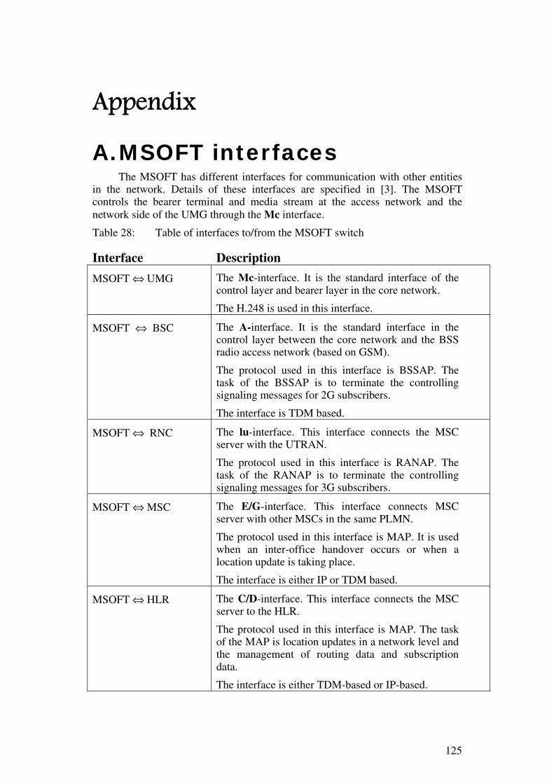
125
Appendix
A. MSOFT interfaces The MSOFT has different interfaces for communication with other entities
in the network. Details of these interfaces are specified in [3]. The MSOFT controls the bearer terminal and media stream at the access network and the network side of the UMG through the Mc interface.
Table 28: Table of interfaces to/from the MSOFT switch
Interface Description
MSOFT ⇔ UMG The Mc-interface. It is the standard interface of the control layer and bearer layer in the core network.
The H.248 is used in this interface.
MSOFT ⇔ BSC The A-interface. It is the standard interface in the control layer between the core network and the BSS radio access network (based on GSM).
The protocol used in this interface is BSSAP. The task of the BSSAP is to terminate the controlling signaling messages for 2G subscribers.
The interface is TDM based.
MSOFT ⇔ RNC The lu-interface. This interface connects the MSC server with the UTRAN.
The protocol used in this interface is RANAP. The task of the RANAP is to terminate the controlling signaling messages for 3G subscribers.
MSOFT ⇔ MSC The E/G-interface. This interface connects MSC server with other MSCs in the same PLMN.
The protocol used in this interface is MAP. It is used when an inter-office handover occurs or when a location update is taking place.
The interface is either IP or TDM based.
MSOFT ⇔ HLR The C/D-interface. This interface connects the MSC server to the HLR.
The protocol used in this interface is MAP. The task of the MAP is location updates in a network level and the management of routing data and subscription data.
The interface is either TDM-based or IP-based.
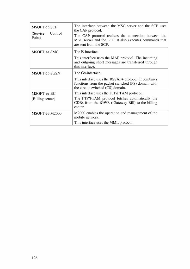
126
MSOFT ⇔ SCP
(Service Control Point)
The interface between the MSC server and the SCP uses the CAP protocol. The CAP protocol realizes the connection between the MSC server and the SCP. It also executes commands that are sent from the SCP.
MSOFT ⇔ SMC The E-interface.
This interface uses the MAP protocol. The incoming and outgoing short messages are transferred through this interface.
MSOFT ⇔ SGSN The Gs-interface.
This interface uses the BSSAP+ protocol. It combines functions from the packet switched (PS) domain with the circuit switched (CS) domain.
MSOFT ⇔ BC (Billing center)
This interface uses the FTP/FTAM protocol. The FTP/FTAM protocol fetches automatically the CDRs from the iGWB (iGateway Bill) to the billing center.
MSOFT ⇔ M2000 M2000 enables the operation and management of the mobile network. This interface uses the MML protocol.

127
B. Call set-up flow diagram Figure 24 shows the flow of ISUP messages when a call is set-up.
When a subscriber calls, a set-up message is first sent to the MSC responsible for that subscriber [27]. The MSC responsible for the calling MS is denoted MSCa and the MSC responsible for the MS that receives the call is denoted MSCb. MSC can be both MSCa and MSCb if the calling MS (MSa) and the MS being called (MSb), both are in the area controlled by the same MSC.
The MSCa sends an IAM (initial address message) to the STP when it has received all the information needed from the MSa and knows that the call is going to be rerouted to another MSC. The IAM contains information needed to reroute the call to the destination MSC (MSCb).
When the MSCb receives the IAM it notifies the MSb.
The MSb responds by sending an alerting indication, which is forwarded as ACM (address complete message) through the network. When the MSCa receives the ACM it sends an alerting indication to the MSa (the calling MS). At this point the subscriber hears the ring back tone.
When the MSb is answered a connect message is sent and forwarded through the network as an ANM (answer message) [27].
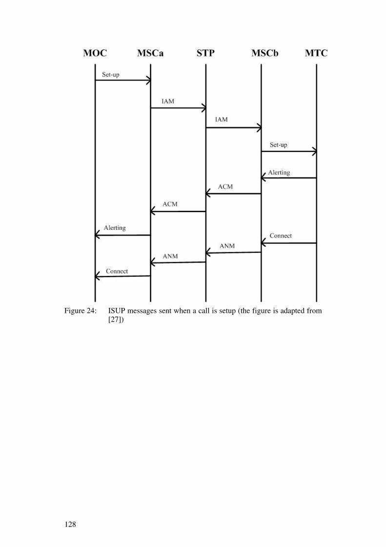
128
Figure 24: ISUP messages sent when a call is setup (the figure is adapted from
[27])
129
C. Measurement entities used in the statistics
C.I Measurement entities for Kulyab traffic
Table 29 gives the measurement entities when collecting statistics from the base stations in Kulyab region. Table 30 gives the measurement entities when collecting statistics from all base station managed by the MSC-RRP. The highlighted areas are those measurement entities used in the analysis.

130
C.II Measurement entities for Kulyab traffic
Table 29: Measurement entities for the statistics collected from base stations in Kulyab region. The highlighted fields are those fields used in the analysis
Measurement entities Number of Local Subscribers (GCI) Number of Roaming Subscribers (GCI) Number of Power-off Subscribers (GCI) Location Update Requested Times (GCI) Location Update Rejected Times (GCI) IMSI Attached Times (GCI) IMSI Detached Times (GCI) MOC Call Attempts (GCI) MOC Released Before Ringing (GCI) MOC Released After Ringing (GCI) MOC Callee Absent Times (GCI) MOC Callee Busy Times (GCI) MOC Connect Times (GCI) MOC Respond Times (GCI) MOC Connect Traffic (GCI) MOC Respond Traffic (GCI) MTC Released Before Ringing (GCI) MTC Released After Ringing (GCI) MTC Connect Times (GCI) MTC Respond Times (GCI) MTC Connect Traffic (GCI) MTC Respond Traffic (GCI) Handover from Cell Times (GCI) Successful Handover from Cell Times (GCI) Handover to Cell Times (GCI) Successful Handover to Cell Times (GCI) Mobile Caller Call Drop Times (GCI) Mobile Callee Call Drop Times (GCI)
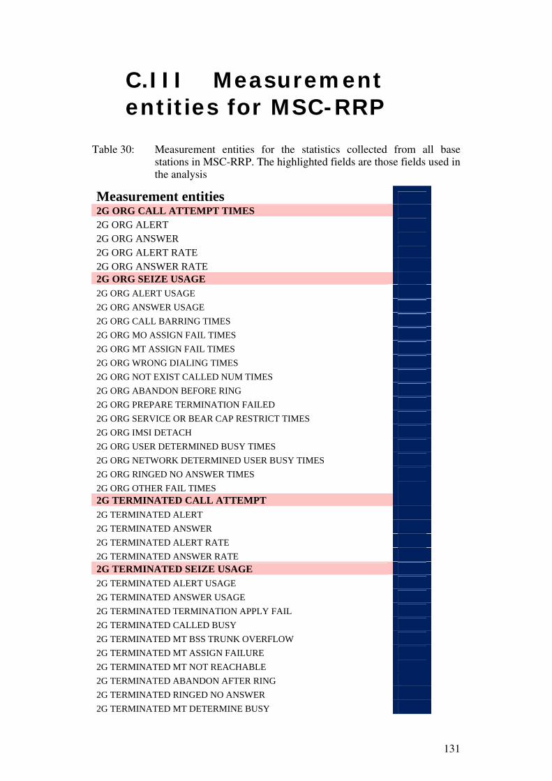
131
C.III Measurement entities for MSC-RRP
Table 30: Measurement entities for the statistics collected from all base stations in MSC-RRP. The highlighted fields are those fields used in the analysis
Measurement entities 2G ORG CALL ATTEMPT TIMES 2G ORG ALERT 2G ORG ANSWER 2G ORG ALERT RATE 2G ORG ANSWER RATE 2G ORG SEIZE USAGE 2G ORG ALERT USAGE 2G ORG ANSWER USAGE 2G ORG CALL BARRING TIMES 2G ORG MO ASSIGN FAIL TIMES 2G ORG MT ASSIGN FAIL TIMES 2G ORG WRONG DIALING TIMES 2G ORG NOT EXIST CALLED NUM TIMES 2G ORG ABANDON BEFORE RING 2G ORG PREPARE TERMINATION FAILED 2G ORG SERVICE OR BEAR CAP RESTRICT TIMES 2G ORG IMSI DETACH 2G ORG USER DETERMINED BUSY TIMES 2G ORG NETWORK DETERMINED USER BUSY TIMES 2G ORG RINGED NO ANSWER TIMES 2G ORG OTHER FAIL TIMES 2G TERMINATED CALL ATTEMPT 2G TERMINATED ALERT 2G TERMINATED ANSWER 2G TERMINATED ALERT RATE 2G TERMINATED ANSWER RATE 2G TERMINATED SEIZE USAGE 2G TERMINATED ALERT USAGE 2G TERMINATED ANSWER USAGE 2G TERMINATED TERMINATION APPLY FAIL 2G TERMINATED CALLED BUSY 2G TERMINATED MT BSS TRUNK OVERFLOW 2G TERMINATED MT ASSIGN FAILURE 2G TERMINATED MT NOT REACHABLE 2G TERMINATED ABANDON AFTER RING 2G TERMINATED RINGED NO ANSWER 2G TERMINATED MT DETERMINE BUSY


133
D. Base stations analyzed for Kulyab region
Table 31: Cells located in LAC 0050 and 0051
436040051311C 4360400505318 43604005154BD 4360400503108 436040051311D 4360400505319 43604005154C5 4360400503109 43604005132A1 4360400505321 43604005154C6 43604005032FB 43604005132A2 4360400505322 43604005154C7 43604005032FC 43604005132A3 4360400505323 4360400515597 43604005032FD 43604005132AB 43604005053A3 4360400515598 4360400503535 43604005132AC 43604005053A4 4360400515599 4360400503536 43604005132AD 43604005053A5 4360400503855 4360400503537 4360400513305 43604005053F3 4360400503856 436040050353F 4360400513306 43604005053F4 4360400503857 4360400503540 4360400513307 43604005053F5 436040050389B 4360400503541 436040051352B 4360400505551 436040050389c 4360400503549 436040051352C 4360400505552 436040050389D 436040050354A 436040051352D 4360400505553 43604005038A5 436040050354B 43604005136ED 436040050558D 43604005038A6 4360400503599 43604005136EE 436040050558E 43604005038A7 436040050359A 43604005136EF 436040050558F 43604005038B9 436040050359B 4360400513805 436040050567D 43604005038BA 436040050384B 4360400513806 436040050567E 43604005038BB 436040050384C 4360400513807 436040050567F 43604005038C3 436040050384D 436040051380F 4360400512757 43604005038C4 4360400503EDB 4360400513810 4360400512758 43604005038C5 4360400503EDC 4360400513811 4360400512759 436040050398B 4360400503EDD4360400513819 43604005128E7 436040050398C 4360400514273 436040051381A 43604005128E8 436040050398D 4360400514274 436040051381B 43604005128E9 4360400503995 4360400514275 436040051382D 4360400512A1D 4360400503996 4360400512B2B 436040051382E 4360400512A1E 4360400503997 4360400512B2C 436040051382F 4360400512A1F 436040050399F 4360400512B2D 4360400513C51 4360400512C39 43604005039A0 4360400513977 4360400513C52 4360400512C3A 43604005039A1 4360400513978 4360400513C53 4360400512C3B 4360400503A0D 4360400513979 4360400513CAB 4360400512E55 4360400503A0E 4360400513EE5 4360400513CAC 4360400512E56 4360400503A0F 4360400513EE6 4360400513CAD 4360400512E57 4360400503C15 4360400513EE7 4360400513E31 4360400512EC3 4360400503C16 4360400515691 4360400513E32 4360400512EC4 4360400503C17 4360400515692 4360400513E33 4360400512EC5 4360400503CBF 4360400515693 4360400513E3B 4360400513071 4360400503CC0 436040051569B
134
4360400513E3C 4360400513072 4360400503CC1 436040051569C 4360400513E3D 4360400513073 4360400503D5F 436040051569D 4360400515083 436040051311B 4360400503D60 43604005028C9 4360400515084 4360400502761 4360400503D61 43604005028CA 4360400515085 4360400502762 4360400503E1D 43604005028CB 4360400515123 4360400502763 4360400503E1E 4360400503F3F 4360400515124 43604005028A1 4360400503E1F 4360400503F40 4360400515125 43604005028A2 4360400503E45 4360400503F41 436040051523B 43604005028A3 4360400503E46 4360400503F8F 436040051523C 43604005028AB 4360400503E47 4360400503F90 436040051523D 43604005028AC 4360400503EC7 4360400503F91 4360400515295 43604005028AD 4360400503EC8 4360400503FB7 4360400515296 43604005028B5 4360400503EC9 4360400503FB8 4360400515297 43604005028B6 4360400505155 4360400503FB9 43604005152DB 43604005028B7 4360400505156 4360400513F35 43604005152DC 4360400502A4F 4360400505157 4360400513F36 4360400515349 4360400502A50 4360400505213 4360400513F37 436040051534A 4360400502A51 4360400505214 4360400513F3F 436040051534B 4360400502A59 4360400505215 4360400513F40 4360400515385 4360400502A5A 436040050526D 4360400513F41 4360400515386 4360400502A5B 436040050526E 4360400513F7B 4360400515387 4360400502F1D 436040050526F 4360400513F7C 436040051538F 4360400502F1E 4360400502F50 4360400513F7D 4360400515390 4360400502F1F 4360400502F58 4360400513FAD 4360400515391 4360400502F4E 4360400502F59 4360400515443 4360400502F4F 4360400502F5A 436040050529F 4360400515444 4360400503085 43604005052A0 4360400515445 4360400503086 43604005052A1 43604005154BB 4360400503087 4360400505317 43604005154BC 4360400503107

135
E. Relative BHCA values Table 32: Relative BHCA values collected from the 23rd of February to 1st of
March 2011. The highest relative BHCA values are highlighted. The unit of BHCA is “call attempts”
Start Time (Hour)
23 of February
24 of February
25 of February
26 of February
27 of February
28 of February
1 of March
0 0.130 0.121 0.129 0.127 0.129 0.121 0.107 1 0.056 0.052 0.060 0.058 0.058 0.051 0.043 2 0.028 0.023 0.029 0.028 0.030 0.024 0.019 3 0.023 0.017 0.019 0.020 0.016 0.020 0.013 4 0.017 0.018 0.014 0.015 0.015 0.017 0.011 5 0.032 0.026 0.031 0.033 0.032 0.029 0.029 6 0.095 0.073 0.082 0.085 0.081 0.081 0.076 7 0.318 0.232 0.227 0.236 0.228 0.223 0.218 8 0.538 0.355 0.365 0.361 0.371 0.344 0.330 9 0.707 0.444 0.483 0.475 0.489 0.436 0.421 10 0.774 0.500 0.543 0.535 0.566 0.491 0.473 11 0.813 0.552 0.552 0.550 0.587 0.526 0.546 12 0.804 0.522 0.501 0.508 0.542 0.593 0.554 13 0.881 0.599 0.576 0.592 0.573 0.604 0.577 14 0.971 0.671 0.675 0.661 0.623 0.660 0.639 15 0.937 0.702 0.714 0.663 0.605 0.637 0.626 16 0.911 0.688 0.671 0.636 0.613 0.605 0.594 17 0.890 0.655 0.619 0.579 0.577 0.518 0.533 18 0.783 0.584 0.559 0.566 0.585 0.513 0.527 19 0.685 0.554 0.513 0.487 0.508 0.482 0.494 20 0.849 0.710 0.679 0.613 0.656 0.677 0.647 21 0.801 0.701 0.661 0.654 0.638 0.656 0.701 22 0.606 0.530 0.514 0.532 0.512 0.497 0.495 23 0.284 0.270 0.269 0.274 0.262 0.238 0.245

136
Table 33: Relative BHCA values collected from the 4th of February to 10th of March 2011
Start Time (Hour)
4 of March
5 of March
6 of March
7 of March
8 of March
9 of March
10 of March
0 0.092 0.094 0.097 0.086 0.098 0.105 0.092 1 0.043 0.044 0.045 0.037 0.045 0.041 0.037 2 0.023 0.024 0.024 0.018 0.024 0.024 0.018 3 0.018 0.014 0.015 0.012 0.016 0.016 0.013 4 0.013 0.014 0.014 0.011 0.013 0.011 0.014 5 0.022 0.023 0.024 0.020 0.023 0.021 0.024 6 0.082 0.082 0.095 0.086 0.123 0.104 0.105 7 0.214 0.206 0.232 0.216 0.398 0.246 0.244 8 0.339 0.327 0.376 0.363 0.700 0.490 0.398 9 0.480 0.449 0.526 0.601 0.992 0.524 0.536 10 0.621 0.564 0.587 0.608 0.924 0.526 0.528 11 0.608 0.581 0.578 0.605 0.912 0.537 0.555 12 0.554 0.564 0.551 0.584 0.829 0.544 0.568 13 0.601 0.594 0.555 0.600 0.815 0.580 0.610 14 0.647 0.609 0.576 0.630 0.808 0.591 0.619 15 0.623 0.590 0.551 0.620 0.770 0.562 0.584 16 0.606 0.567 0.530 0.563 0.699 0.538 0.549 17 0.555 0.512 0.523 0.529 0.598 0.495 0.522 18 0.449 0.508 0.478 0.495 0.594 0.472 0.499 19 0.433 0.456 0.426 0.459 0.643 0.469 0.480 20 0.596 0.576 0.582 0.605 0.750 0.571 0.591 21 0.709 0.698 0.714 0.768 0.906 0.739 0.761 22 0.496 0.507 0.486 0.522 0.616 0.487 0.469 23 0.223 0.232 0.219 0.226 0.265 0.213 0.200

137
Table 34: Relative BHCA values collected from the 11th of March to 15th of March 2011
Start Time (Hour)
11 of March
12 of March
13 of March
14 of March
15 of March
0 0.077 0.073 0.078 0.075 0.069 1 0.035 0.034 0.038 0.030 0.030 2 0.020 0.018 0.019 0.017 0.018 3 0.013 0.012 0.015 0.013 0.010 4 0.014 0.014 0.015 0.013 0.010 5 0.031 0.024 0.025 0.027 0.023 6 0.107 0.113 0.121 0.117 0.100 7 0.250 0.263 0.273 0.273 0.247 8 0.442 0.424 0.500 0.480 0.483 9 0.518 0.538 0.594 0.503 0.502 10 0.524 0.530 0.580 0.512 0.516 11 0.551 0.544 0.574 0.524 0.527 12 0.533 0.537 0.566 0.539 0.509 13 0.586 0.579 0.587 0.583 0.558 14 0.639 0.581 0.570 0.590 0.567 15 0.583 0.578 0.547 0.559 0.558 16 0.546 0.528 0.516 0.495 0.543 17 0.489 0.497 0.457 0.455 0.532 18 0.487 0.504 0.462 0.448 0.506 19 0.490 0.474 0.447 0.450 0.373 20 0.617 0.600 0.564 0.601 0.722 21 0.811 0.797 0.814 0.835 0.675 22 0.430 0.417 0.422 0.421 0.316 23 0.181 0.179 0.174 0.176 0.138

138
Table 35: Relative BHCA values collected from the 18th of March to 25th of March 2011
Start Time (Hour)
18 of March
19 of March
20 of March
21 of March
22 of March
23 of March
24 of March
25 of March
0 0.069 0.057 0.076 0.084 0.098 0.058 0.053 0.035 1 0.029 0.025 0.030 0.035 0.038 0.024 0.022 0.014 2 0.020 0.015 0.019 0.017 0.016 0.012 0.013 0.009 3 0.011 0.011 0.013 0.010 0.011 0.007 0.011 0.005 4 0.012 0.011 0.014 0.011 0.012 0.007 0.011 0.006 5 0.025 0.027 0.029 0.023 0.027 0.021 0.022 0.016 6 0.108 0.111 0.150 0.159 0.203 0.164 0.165 0.103 7 0.257 0.266 0.341 0.398 0.492 0.384 0.373 0.222 8 0.527 0.556 0.493 0.582 0.645 0.533 0.493 0.277 9 0.518 0.547 0.491 0.589 0.606 0.539 0.495 0.311 10 0.512 0.515 0.473 0.554 0.534 0.500 0.458 0.316 11 0.517 0.506 0.450 0.552 0.518 0.476 0.436 0.319 12 0.502 0.499 0.440 0.531 0.531 0.473 0.432 0.306 13 0.532 0.529 0.449 0.538 0.558 0.493 0.453 0.324 14 0.573 0.526 0.458 0.545 0.544 0.497 0.459 0.351 15 0.543 0.509 0.431 0.506 0.513 0.477 0.429 0.336 16 0.511 0.483 0.415 0.465 0.494 0.442 0.400 0.317 17 0.465 0.463 0.386 0.432 0.472 0.402 0.377 0.297 18 0.492 0.483 0.405 0.467 0.469 0.422 0.384 0.316 19 0.385 0.407 0.367 0.488 0.450 0.459 0.461 0.357 20 0.693 0.467 0.438 0.442 0.490 0.380 0.353 0.345 21 0.697 0.797 0.694 0.600 0.866 0.847 0.402 0.337 22 0.323 0.452 0.531 0.712 0.387 0.405 0.213 0.194 23 0.128 0.193 0.221 0.277 0.153 0.152 0.086 0.087

139
F. Relative values of the connect traffic Table 36, Table 37, Table 38, and Table 39 give the relative connected
traffic in the measurement period 23rd of February to 25th of March 2011. The highest daily value for the relative connected traffic is highlighted. The unit of connected traffic is in Erlangs; therefore the unit of relative connected traffic is Erlangs/Erlangs, as the relative connected traffic relates to the highest measured value for connected traffic in the current measurement period.
Table 36: Values of the relative connected traffic collected from the 23rd of February to 1st of March 2011
Start Time
23rd of February
24th of February
25th of February
26th of February
27th of February
28th of February
1st of March
(Hour)
0 0.148 0.148 0.153 0.147 0.155 0.139 0.124 1 0.059 0.058 0.070 0.063 0.071 0.061 0.050 2 0.028 0.026 0.026 0.029 0.036 0.028 0.024 3 0.019 0.015 0.015 0.017 0.019 0.017 0.015 4 0.014 0.015 0.011 0.013 0.015 0.014 0.010 5 0.023 0.019 0.023 0.024 0.025 0.020 0.021 6 0.084 0.065 0.071 0.073 0.075 0.067 0.071 7 0.325 0.264 0.265 0.263 0.262 0.243 0.251 8 0.596 0.447 0.460 0.453 0.454 0.420 0.415 9 0.746 0.560 0.597 0.592 0.593 0.535 0.536 10 0.784 0.616 0.646 0.634 0.668 0.586 0.593 11 0.803 0.674 0.646 0.625 0.673 0.607 0.654 12 0.765 0.604 0.569 0.559 0.633 0.648 0.635 13 0.812 0.662 0.633 0.639 0.657 0.650 0.655 14 0.875 0.735 0.743 0.709 0.700 0.686 0.720 15 0.854 0.752 0.759 0.726 0.699 0.664 0.701 16 0.848 0.764 0.733 0.724 0.728 0.634 0.680 17 0.866 0.763 0.715 0.688 0.708 0.568 0.628 18 0.830 0.701 0.682 0.693 0.747 0.566 0.646 19 0.814 0.743 0.699 0.679 0.732 0.601 0.700 20 0.944 0.892 0.859 0.800 0.873 0.764 0.862 21 0.878 0.834 0.773 0.781 0.822 0.722 0.825 22 0.663 0.625 0.576 0.601 0.609 0.537 0.577 23 0.337 0.334 0.304 0.312 0.307 0.267 0.273
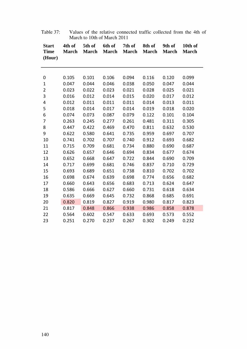
140
Table 37: Values of the relative connected traffic collected from the 4th of March to 10th of March 2011
Start Time
4th of March
5th of March
6th of March
7th of March
8th of March
9th of March
10th of March
(Hour)
0 0.105 0.101 0.106 0.094 0.116 0.120 0.099 1 0.047 0.044 0.046 0.038 0.050 0.047 0.044 2 0.023 0.022 0.023 0.021 0.028 0.025 0.021 3 0.016 0.012 0.014 0.015 0.020 0.017 0.012 4 0.012 0.011 0.011 0.011 0.014 0.013 0.011 5 0.018 0.014 0.017 0.014 0.019 0.018 0.020 6 0.074 0.073 0.087 0.079 0.122 0.101 0.104 7 0.263 0.245 0.277 0.261 0.481 0.311 0.305 8 0.447 0.422 0.469 0.470 0.811 0.632 0.530 9 0.622 0.580 0.641 0.735 0.959 0.697 0.707 10 0.741 0.702 0.707 0.740 0.912 0.693 0.682 11 0.715 0.709 0.681 0.734 0.880 0.690 0.687 12 0.626 0.657 0.646 0.694 0.834 0.677 0.674 13 0.652 0.668 0.647 0.722 0.844 0.690 0.709 14 0.717 0.699 0.681 0.746 0.837 0.710 0.729 15 0.693 0.689 0.651 0.738 0.810 0.702 0.702 16 0.698 0.674 0.639 0.698 0.774 0.656 0.682 17 0.660 0.643 0.656 0.683 0.713 0.624 0.647 18 0.586 0.666 0.627 0.660 0.731 0.618 0.634 19 0.635 0.669 0.645 0.732 0.868 0.685 0.691 20 0.820 0.819 0.827 0.919 0.980 0.817 0.823 21 0.817 0.848 0.866 0.938 0.986 0.858 0.878 22 0.564 0.602 0.547 0.633 0.693 0.573 0.552 23 0.251 0.270 0.237 0.267 0.302 0.249 0.232

141
Table 38: Values of the relative connected traffic collected from the 11th of March to 15th of March 2011
Start Time
11th of March
12th of March
13th of March
14th of March
15th of March
(Hour)
0 0.088 0.089 0.093 0.088 0.085 1 0.037 0.042 0.043 0.034 0.038 2 0.019 0.021 0.019 0.018 0.020 3 0.011 0.013 0.013 0.014 0.012 4 0.012 0.013 0.012 0.012 0.009 5 0.023 0.019 0.019 0.018 0.016 6 0.107 0.117 0.126 0.124 0.104 7 0.315 0.330 0.347 0.350 0.306 8 0.579 0.554 0.618 0.638 0.621 9 0.681 0.696 0.729 0.669 0.653 10 0.678 0.674 0.712 0.667 0.659 11 0.678 0.678 0.693 0.675 0.658 12 0.633 0.647 0.676 0.654 0.615 13 0.684 0.681 0.693 0.692 0.664 14 0.745 0.705 0.699 0.712 0.676 15 0.711 0.702 0.667 0.681 0.661 16 0.671 0.654 0.637 0.627 0.648 17 0.619 0.629 0.585 0.589 0.666 18 0.629 0.649 0.597 0.580 0.636 19 0.701 0.699 0.654 0.662 0.581 20 0.840 0.826 0.797 0.838 0.888 21 0.910 0.890 0.892 0.927 0.783 22 0.510 0.497 0.517 0.516 0.387 23 0.214 0.220 0.217 0.213 0.170
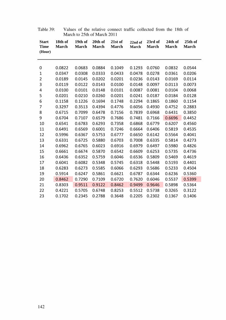
142
Table 39: Values of the relative connect traffic collected from the 18th of March to 25th of March 2011
Start Time
18th of March
19th of March
20th of March
21st of March
22nd of March
23rd of March
24th of March
25th of March
(Hour)
0 0.0822 0.0683 0.0884 0.1049 0.1293 0.0760 0.0832 0.0544 1 0.0347 0.0308 0.0333 0.0433 0.0478 0.0278 0.0361 0.0206 2 0.0189 0.0145 0.0202 0.0201 0.0236 0.0143 0.0169 0.0114 3 0.0119 0.0122 0.0143 0.0100 0.0148 0.0097 0.0113 0.0073 4 0.0100 0.0101 0.0148 0.0101 0.0087 0.0081 0.0104 0.0068 5 0.0201 0.0210 0.0260 0.0201 0.0241 0.0187 0.0184 0.0128 6 0.1158 0.1226 0.1694 0.1748 0.2294 0.1865 0.1860 0.1154 7 0.3297 0.3513 0.4394 0.4776 0.6056 0.4930 0.4752 0.2883 8 0.6715 0.7099 0.6478 0.7156 0.7839 0.6968 0.6431 0.3850 9 0.6704 0.7107 0.6579 0.7686 0.7481 0.7166 0.6696 0.4452 10 0.6541 0.6783 0.6293 0.7358 0.6868 0.6779 0.6207 0.4560 11 0.6491 0.6569 0.6001 0.7246 0.6664 0.6406 0.5819 0.4535 12 0.5996 0.6367 0.5753 0.6777 0.6650 0.6142 0.5564 0.4041 13 0.6331 0.6725 0.5880 0.6703 0.7008 0.6335 0.5814 0.4273 14 0.6962 0.6765 0.6023 0.6916 0.6979 0.6497 0.5980 0.4826 15 0.6661 0.6674 0.5870 0.6542 0.6609 0.6253 0.5735 0.4736 16 0.6436 0.6352 0.5759 0.6046 0.6536 0.5809 0.5469 0.4619 17 0.6041 0.6082 0.5348 0.5745 0.6318 0.5448 0.5193 0.4401 18 0.6283 0.6273 0.5585 0.6066 0.6293 0.5686 0.5233 0.4504 19 0.5914 0.6247 0.5861 0.6621 0.6787 0.6344 0.6236 0.5360 20 0.8462 0.7290 0.7109 0.6720 0.7620 0.6046 0.5537 0.5399 21 0.8303 0.9511 0.9122 0.8462 0.9499 0.9646 0.5898 0.5364 22 0.4221 0.5705 0.6748 0.8253 0.5512 0.5738 0.3265 0.3122 23 0.1702 0.2345 0.2788 0.3648 0.2205 0.2302 0.1367 0.1406
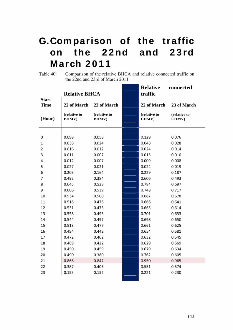
143
G. Comparison of the traffic on the 22nd and 23rd March 2011
Table 40: Comparison of the relative BHCA and relative connected traffic on the 22nd and 23rd of March 2011
Relative BHCA Relative connected traffic
Start Time 22 of March 23 of March 22 of March 23 of March
(Hour) (relative to BHMV)
(relative to BHMV)
(relative to CHMV)
(relative to CHMV)
0 0.098 0.058 0.129 0.076 1 0.038 0.024 0.048 0.028 2 0.016 0.012 0.024 0.014 3 0.011 0.007 0.015 0.010 4 0.012 0.007 0.009 0.008 5 0.027 0.021 0.024 0.019 6 0.203 0.164 0.229 0.187 7 0.492 0.384 0.606 0.493 8 0.645 0.533 0.784 0.697 9 0.606 0.539 0.748 0.717 10 0.534 0.500 0.687 0.678 11 0.518 0.476 0.666 0.641 12 0.531 0.473 0.665 0.614 13 0.558 0.493 0.701 0.633 14 0.544 0.497 0.698 0.650 15 0.513 0.477 0.661 0.625 16 0.494 0.442 0.654 0.581 17 0.472 0.402 0.632 0.545 18 0.469 0.422 0.629 0.569 19 0.450 0.459 0.679 0.634 20 0.490 0.380 0.762 0.605 21 0.866 0.847 0.950 0.965 22 0.387 0.405 0.551 0.574 23 0.153 0.152 0.221 0.230


145
H. The traffic measured the 23rd of February
Table 41: Traffic load the 23rd of February 2011
Start time
Relative BHCA
Relative connected traffic
Relative response traffic
(Hour) (relates to BHMV)
(relates to CHMV)
(relates to CHMV)
0 0.129548315 0.148376 0.126831579 1 0.055750191 0.058713 0.050197368 2 0.028473787 0.028105 0.023357895 3 0.022689101 0.019089 0.015965789 4 0.017498371 0.014024 0.011471053 5 0.032011034 0.022721 0.015865789 6 0.094726764 0.083761 0.056405263 7 0.317817157 0.324576 0.226984211 8 0.53847218 0.595842 0.430621053 9 0.70672591 0.746355 0.545410526 10 0.774332079 0.784182 0.571473684 11 0.812735921 0.803447 0.583552632 12 0.803516416 0.765216 0.544794737 13 0.880799933 0.812037 0.583828947 14 0.970952876 0.874711 0.638123684 15 0.937365787 0.854321 0.621357895 16 0.91073173 0.847811 0.614736842 17 0.89044882 0.866279 0.631734211 18 0.782680865 0.830142 0.606523684 19 0.685348 0.814387 0.614102632 20 0.849096798 0.943913 0.740142105 21 0.800937045 0.877997 0.696702632 22 0.606111921 0.662563 0.529939474 23 0.283773337 0.336742 0.279778947

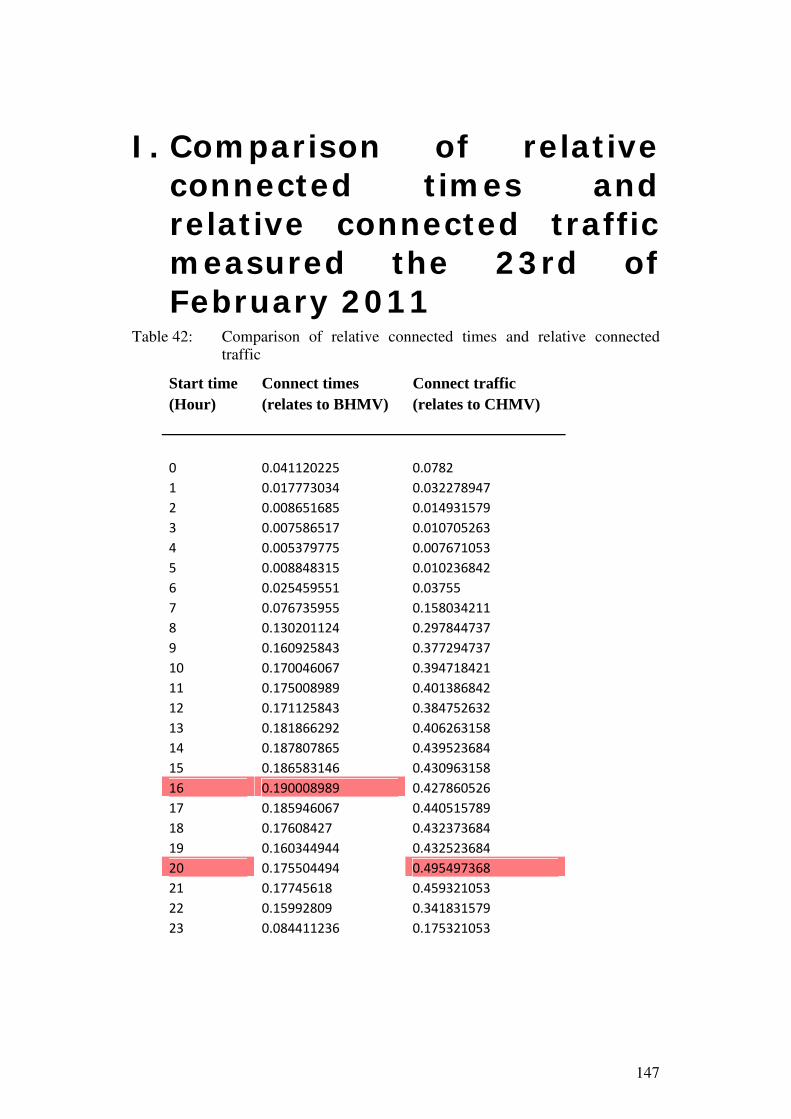
147
I. Comparison of relative connected times and relative connected traffic measured the 23rd of February 2011
Table 42: Comparison of relative connected times and relative connected traffic
Start time Connect times Connect traffic (Hour) (relates to BHMV) (relates to CHMV)
0 0.041120225 0.0782 1 0.017773034 0.032278947 2 0.008651685 0.014931579 3 0.007586517 0.010705263 4 0.005379775 0.007671053 5 0.008848315 0.010236842 6 0.025459551 0.03755 7 0.076735955 0.158034211 8 0.130201124 0.297844737 9 0.160925843 0.377294737 10 0.170046067 0.394718421 11 0.175008989 0.401386842 12 0.171125843 0.384752632 13 0.181866292 0.406263158 14 0.187807865 0.439523684 15 0.186583146 0.430963158 16 0.190008989 0.427860526 17 0.185946067 0.440515789 18 0.17608427 0.432373684 19 0.160344944 0.432523684 20 0.175504494 0.495497368 21 0.17745618 0.459321053 22 0.15992809 0.341831579 23 0.084411236 0.175321053


149
J. Maximum values for relative BHCA and relative connected traffic
Table 43: Maximum values for relative BHCA and relative connected traffic in Kulyab
Date
Maximum relative BHCA
Maximum relative connected traffic weekday
(month-day)
Feb. 23 0.970952876 0.943913158 Wednesday 24 0.710387504 0.891671053 Thursday 25 0.71372145 0.85905 Friday 26 0.663193599 0.800039474 Saturday 27 0.655556214 0.872873684 Sunday 28 0.677215832 0.764392105 Monday March 1 0.701394825 0.862405263 Tuesday 2 3 4 0.709481818 0.819826316 Friday 5 0.698293973 0.848384211 Saturday 6 0.713569016 0.865992105 Sunday 7 0.767953286 0.938307895 Monday 8 0.991592169 0.986015789 Tuesday 9 0.739108206 0.858244737 Wednesday 10 0.761434627 0.878047368 Thursday 11 0.811031018 0.909818421 Friday 12 0.797133265 0.889805263 Saturday 13 0.813681342 0.892189474 Sunday 14 0.835312019 0.927263158 Monday 15 0.722487913 0.888239474 Tuesday 16 17 18 0.696862649 0.846192105 Friday 19 0.797370242 0.9511 Saturday 20 0.694201362 0.912221053 Sunday 21 0.712041607 0.8462 Monday 22 0.866464556 0.949897368 Tuesday

150
23 0.846877732 0.964602632 Wednesday 24 0.495468233 0.669610526 Thursday 25 0.357382942 0.539942105 Friday

151
K. The hour when there is a peak
Table 44: Hour when the daily peaks take place
Relative BHCA
Relative connected traffic
Relative response traffic
Date
Start Time (relates to
BHMV) (relates to CHMV)
(relates to CHMV)
(Hour)
February 23rd 14 0.970952876 0.874710526 0.638123684
20 0.849096798 0.943913158 0.740142105
24th 20 0.710387504 0.891671053 0.712828947
25th 15 0.71372145 0.759455263 0.562547368 20 0.679058733 0.85905 0.689481579
26th 15 0.663193599 0.726018421 0.537068421 20 0.613432584 0.800039474 0.636560526
27th 20 0.655556214 0.872873684 0.704271053
28th 20 0.677215832 0.764392105 0.616694737
March 1st 20 0.647249132 0.862405263 0.697297368
21 0.701394825 0.825242105 0.669431579
4th 20 0.595842663 0.819826316 0.663573684 21 0.709481818 0.816589474 0.662957895
5th 21 0.698293973 0.848384211 0.686202632
6th 21 0.713569016 0.865992105 0.705494737
7th 21 0.767953286 0.938307895 0.76945
8th 9 0.991592169 0.959039474 0.717184211

152
21 0.905563602 0.986015789 0.774965789
9th 21 0.739108206 0.858244737 0.682831579
10th 21 0.761434627 0.878047368 0.708968421
11th 21 0.811031018 0.909818421 0.735328947
12th 21 0.797133265 0.889805263 0.723878947
13th 21 0.813681342 0.892189474 0.725681579
14th 21 0.835312019 0.927263158 0.76215
15th 20 0.722487913 0.888239474 0.712886842
18th 20 0.693198808 0.846192105 0.673534211 21 0.696862649 0.830252632 0.688089474
19th 21 0.797370242 0.9511 0.776739474
20th 21 0.694201362 0.912221053 0.740481579
21st 21 0.600262887 0.8462 0.671744737 22 0.712041607 0.825339474 0.669073684
22nd 21 0.866464556 0.949897368 0.763392105
23rd 21 0.846877732 0.964602632 0.783897368
24th 9 0.495468233 0.669610526 0.481994737
25th 19 0.357382942 0.535994737 0.415915789 20 0.345113041 0.539942105 0.431560526 21 0.336661083 0.536415789 0.447686842
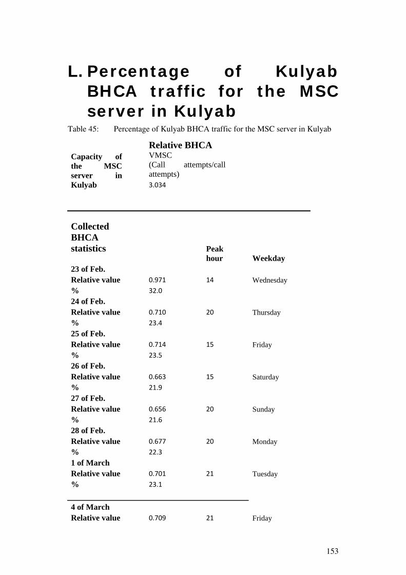
153
L. Percentage of Kulyab BHCA traffic for the MSC server in Kulyab
Table 45: Percentage of Kulyab BHCA traffic for the MSC server in Kulyab
Capacity of the MSC server in Kulyab
Relative BHCA VMSC (Call attempts/call attempts)3.034
Collected BHCA statistics
Peak hour Weekday
23 of Feb. Relative value 0.971 14 Wednesday % 32.0 24 of Feb. Relative value 0.710 20 Thursday % 23.4 25 of Feb. Relative value 0.714 15 Friday % 23.5 26 of Feb. Relative value 0.663 15 Saturday % 21.9 27 of Feb. Relative value 0.656 20 Sunday % 21.6 28 of Feb. Relative value 0.677 20 Monday % 22.3 1 of March Relative value 0.701 21 Tuesday % 23.1 4 of March Relative value 0.709 21 Friday
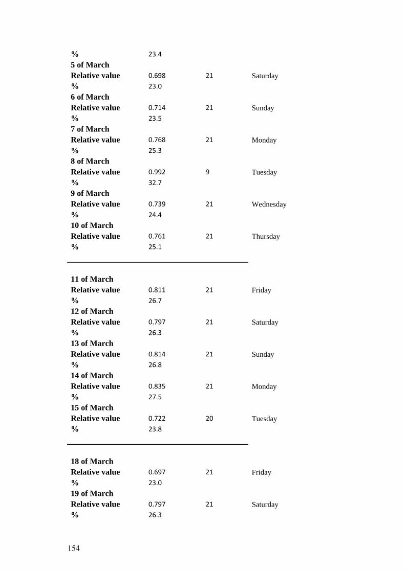
154
% 23.4 5 of March Relative value 0.698 21 Saturday % 23.0 6 of March Relative value 0.714 21 Sunday % 23.5 7 of March Relative value 0.768 21 Monday % 25.3 8 of March Relative value 0.992 9 Tuesday % 32.7 9 of March Relative value 0.739 21 Wednesday % 24.4 10 of March Relative value 0.761 21 Thursday % 25.1
11 of March Relative value 0.811 21 Friday % 26.7 12 of March Relative value 0.797 21 Saturday % 26.3 13 of March Relative value 0.814 21 Sunday % 26.8 14 of March Relative value 0.835 21 Monday % 27.5 15 of March Relative value 0.722 20 Tuesday % 23.8
18 of March Relative value 0.697 21 Friday % 23.0 19 of March Relative value 0.797 21 Saturday % 26.3

155
20 of March Relative value 0.694 21 Sunday % 22.9 21 of March Relative value 0.712 22 Monday % 23.5 22 of March Relative value 0.866 21 Tuesday % 28. 6 23 of March Relative value 0.847 21 Wednesday % 27.9
24 of March Relative value 0.495 9 Thursday % 16.3 25 of March Relative value 0.357 19 Friday % 11.8

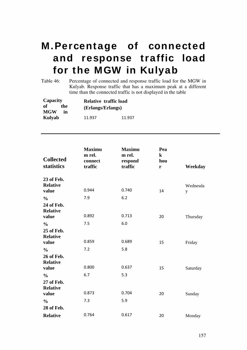
157
M. Percentage of connected and response traffic load for the MGW in Kulyab
Table 46: Percentage of connected and response traffic load for the MGW in Kulyab. Response traffic that has a maximum peak at a different time than the connected traffic is not displayed in the table
Capacity of the MGW in Kulyab
Relative traffic load (Erlangs/Erlangs)
11.937 11.937
Collected statistics
Maximum rel. connect traffic
Maximum rel. respond traffic
Peak hour Weekday
23 of Feb. Relative value 0.944 0.740 14
Wednesday
% 7.9 6.2
24 of Feb. Relative value 0.892 0.713 20 Thursday
% 7.5 6.0
25 of Feb. Relative value 0.859 0.689 15 Friday
% 7.2 5.8
26 of Feb. Relative value 0.800 0.637 15 Saturday
% 6.7 5.3
27 of Feb. Relative value 0.873 0.704 20 Sunday
% 7.3 5.9
28 of Feb. Relative 0.764 0.617 20 Monday
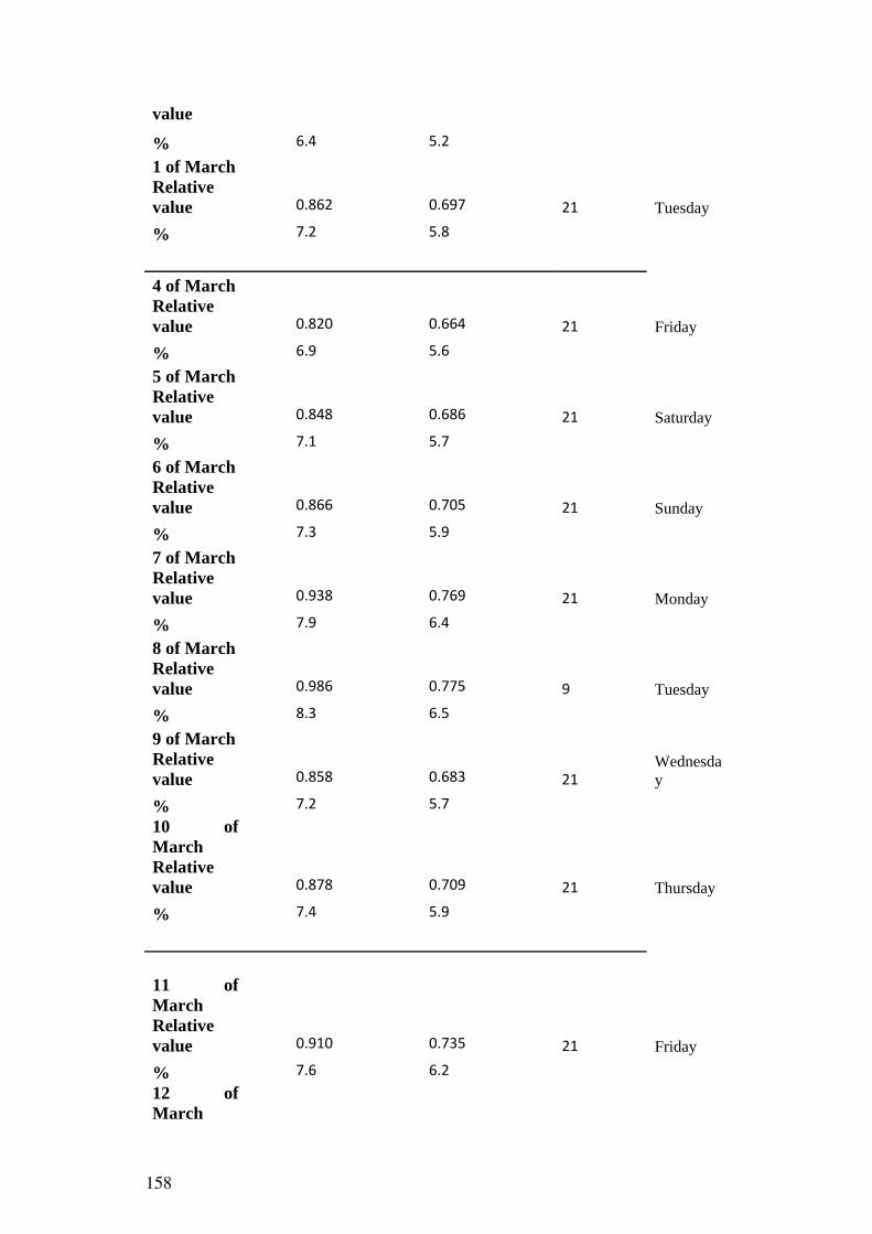
158
value
% 6.4 5.2
1 of March Relative value 0.862 0.697 21 Tuesday
% 7.2 5.8
4 of March Relative value 0.820 0.664 21 Friday
% 6.9 5.6
5 of March Relative value 0.848 0.686 21 Saturday
% 7.1 5.7
6 of March Relative value 0.866 0.705 21 Sunday
% 7.3 5.9
7 of March Relative value 0.938 0.769 21 Monday
% 7.9 6.4
8 of March Relative value 0.986 0.775 9 Tuesday
% 8.3 6.5
9 of March Relative value 0.858 0.683 21
Wednesday
% 7.2 5.7 10 of March Relative value 0.878 0.709 21 Thursday
% 7.4 5.9
11 of March Relative value 0.910 0.735 21 Friday
% 7.6 6.2 12 of March

159
Relative value 0.890 0.724 21 Saturday
% 7.5 6.1 13 of March Relative value 0.892 0.726 21 Sunday
% 7.5 6.1 14 of March Relative value 0.927 0.762 21 Monday
% 7.8 6.4 15 of March Relative value 0.888 0.713 20 Tuesday
% 7.4 6.0
18 of March Relative value 0.846 21 Friday
% 7.1 19 of March Relative value 0.951 0.777 21 Saturday
% 8.0 6.5 20 of March Relative value 0.912 0.740 21 Sunday
% 7.6 6.2 21 of March Relative value 0.846 0.672 22 Monday
% 7.1 5.6 22 of March Relative value 0.950 0.763 21 Tuesday
% 8.0 6.4 23 of March

160
Relative value 0.965 0.784 21
Wednesday
% 8.1 6.6
24 of March Relative value 0.670 0.482 9 Thursday
% 5.6 4.0 25 of March Relative value 0.540 19 Friday
% 4.5

161
N. Kulyab traffic the 17th of May 2011
Table 47: Highest measured values for the period 16th of May to 22nd of May 2011
Relative percentage of Kulyab traffic in MSC-RRP
Start time
Relative BHCA
Relative connected traffic BHCA
connected traffic
(Hour)
(Call attempts/ call attempts) (Erlangs/Erlangs)
(relative %)
(relative %)
0 0.156247191 0.2274 67.93481 91.01381 1 0.069423596 0.094226316 72.0965 87.85299 2 0.027403371 0.030923684 74.674 74.74054 3 0.014896629 0.014389474 67.99075 61.69403 4 0.017461798 0.017384211 51.92235 53.68912 5 0.077822472 0.099044737 56.40986 73.37632 6 0.192506742 0.275794737 58.28314 83.04168 7 0.311937079 0.485428947 61.77761 91.46805 8 0.368526966 0.572236842 62.26549 90.13241 9 0.388051685 0.629073684 62.6875 92.67813 10 0.414491011 0.671207895 61.64528 92.96488 11 0.437644944 0.683886842 62.65871 92.62708 12 0.43677191 0.661326316 61.34246 90.97905 13 0.483220225 0.687463158 61.69507 89.21174 14 0.477862921 0.687576316 61.59645 89.07692 15 0.456461798 0.676168421 61.65223 89.46372 16 0.450864045 0.687334211 62.88695 91.26263 17 0.435286517 0.687186842 63.44792 92.84559 18 0.415714607 0.677628947 62.66978 93.45005 19 0.463105618 0.731310526 63.5318 93.79327 20 0.519548315 0.897913158 61.79354 95.23855 21 0.59241236 0.967273684 57.15796 89.32745 22 0.53162809 0.828171053 60.02197 89.95022 23 0.316616854 0.489368421 64.37 91.87272


163
O. Calculation of the capacity increase for MSC-RRP
Capacity of MSC-RRP as configured: C Capacity of the traffic : T1 T1=Tk+T2 (generated in MSC-RRP) -> T2=T1-Tk Capacity of the Traffic concerning Kulyab region: Tk
Capacity of traffic in MSC-RRP: (excluding the Kulyab traffic) T2
The free capacity of the MSC-RRP: (including Kulyab traffic)
F1=C-T1
The free capacity of the MSC-RRP:
F2=C-T2
(excluding Kulyab traffic)
The increased capacity for MSC-RRP: I=F2/F1 = (C-T2)/(C-T1)
=(C-T1+Tk)/(C-T1)


165
The ratio between connect times and seizure times for incoming trunk group the 26th of March
Relative Relative Ratio (times):
Object Instance Start Time seizure times connected times
Connect/Seizure
(Incoming trunk group--ATS-27(3))
2011-03-26 00:00:00+05:00 0.0376 0.0348 0.9241
(Incoming trunk group--ATS-27(3))
2011-03-26 01:00:00+05:00 0.0190 0.0176 0.9250
(Incoming trunk group--ATS-27(3))
2011-03-26 02:00:00+05:00 0.0076 0.0071 0.9375
(Incoming trunk group--ATS-27(3))
2011-03-26 03:00:00+05:00 0.0048 0.0048 1.0000
(Incoming trunk group--ATS-27(3))
2011-03-26 04:00:00+05:00 0.0010 0.0010 1.0000
(Incoming trunk group--ATS-27(3))
2011-03-26 05:00:00+05:00 0.0100 0.0081 0.8095
(Incoming trunk group--ATS-27(3))
2011-03-26 06:00:00+05:00 0.1205 0.1052 0.8735
(Incoming trunk group--ATS-27(3))
2011-03-26 07:00:00+05:00 0.4014 0.3600 0.8968
(Incoming trunk group--ATS-27(3))
2011-03-26 08:00:00+05:00 0.8362 0.7238 0.8656
(Incoming trunk group--ATS-27(3))
2011-03-26 09:00:00+05:00 1.1819 1.0414 0.8811
(Incoming trunk group--ATS-27(3))
2011-03-26 10:00:00+05:00 1.1471 1.0043 0.8755
(Incoming trunk group--ATS-27(3))
2011-03-26 11:00:00+05:00 1.1262 0.9910 0.8799
(Incoming trunk group--ATS-27(3))
2011-03-26 12:00:00+05:00 0.9400 0.8324 0.8855
(Incoming trunk group--ATS-27(3))
2011-03-26 13:00:00+05:00 0.7962 0.6924 0.8696
(Incoming trunk group--ATS-27(3))
2011-03-26 14:00:00+05:00 0.7414 0.6481 0.8741
(Incoming trunk group--ATS-27(3))
2011-03-26 15:00:00+05:00 0.7295 0.6438 0.8825
(Incoming trunk group--ATS-27(3))
2011-03-26 16:00:00+05:00 0.7005 0.6095 0.8702
(Incoming trunk group--ATS-27(3))
2011-03-26 17:00:00+05:00 0.6124 0.5324 0.8694
(Incoming trunk group--ATS-27(3))
2011-03-26 18:00:00+05:00 0.6105 0.5405 0.8853
(Incoming trunk group--ATS-27(3))
2011-03-26 19:00:00+05:00 0.5367 0.4748 0.8846
(Incoming trunk group--ATS-27(3))
2011-03-26 20:00:00+05:00 0.5238 0.4414 0.8427
(Incoming trunk group--ATS-27(3))
2011-03-26 21:00:00+05:00 0.3586 0.3181 0.8871
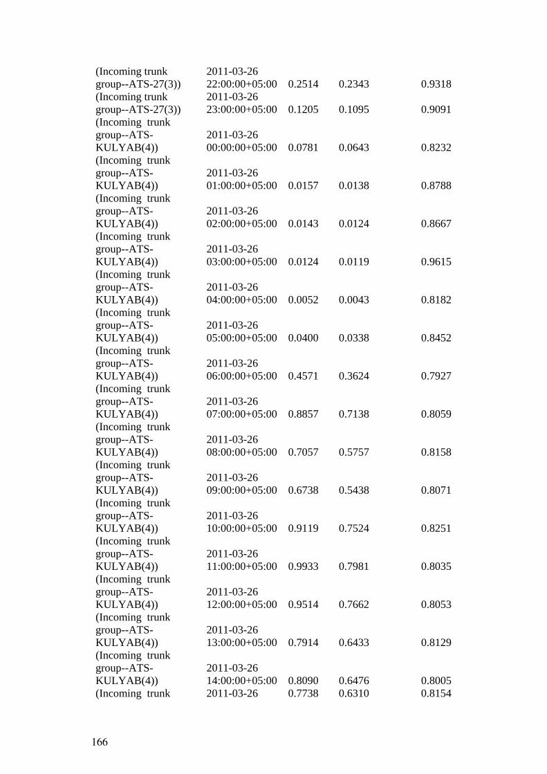
166
(Incoming trunk group--ATS-27(3))
2011-03-26 22:00:00+05:00 0.2514 0.2343 0.9318
(Incoming trunk group--ATS-27(3))
2011-03-26 23:00:00+05:00 0.1205 0.1095 0.9091
(Incoming trunk group--ATS-KULYAB(4))
2011-03-26 00:00:00+05:00 0.0781 0.0643 0.8232
(Incoming trunk group--ATS-KULYAB(4))
2011-03-26 01:00:00+05:00 0.0157 0.0138 0.8788
(Incoming trunk group--ATS-KULYAB(4))
2011-03-26 02:00:00+05:00 0.0143 0.0124 0.8667
(Incoming trunk group--ATS-KULYAB(4))
2011-03-26 03:00:00+05:00 0.0124 0.0119 0.9615
(Incoming trunk group--ATS-KULYAB(4))
2011-03-26 04:00:00+05:00 0.0052 0.0043 0.8182
(Incoming trunk group--ATS-KULYAB(4))
2011-03-26 05:00:00+05:00 0.0400 0.0338 0.8452
(Incoming trunk group--ATS-KULYAB(4))
2011-03-26 06:00:00+05:00 0.4571 0.3624 0.7927
(Incoming trunk group--ATS-KULYAB(4))
2011-03-26 07:00:00+05:00 0.8857 0.7138 0.8059
(Incoming trunk group--ATS-KULYAB(4))
2011-03-26 08:00:00+05:00 0.7057 0.5757 0.8158
(Incoming trunk group--ATS-KULYAB(4))
2011-03-26 09:00:00+05:00 0.6738 0.5438 0.8071
(Incoming trunk group--ATS-KULYAB(4))
2011-03-26 10:00:00+05:00 0.9119 0.7524 0.8251
(Incoming trunk group--ATS-KULYAB(4))
2011-03-26 11:00:00+05:00 0.9933 0.7981 0.8035
(Incoming trunk group--ATS-KULYAB(4))
2011-03-26 12:00:00+05:00 0.9514 0.7662 0.8053
(Incoming trunk group--ATS-KULYAB(4))
2011-03-26 13:00:00+05:00 0.7914 0.6433 0.8129
(Incoming trunk group--ATS-KULYAB(4))
2011-03-26 14:00:00+05:00 0.8090 0.6476 0.8005
(Incoming trunk 2011-03-26 0.7738 0.6310 0.8154

167
group--ATS-KULYAB(4))
15:00:00+05:00
(Incoming trunk group--ATS-KULYAB(4))
2011-03-26 16:00:00+05:00 0.7067 0.5671 0.8026
(Incoming trunk group--ATS-KULYAB(4))
2011-03-26 17:00:00+05:00 0.8157 0.6567 0.8050
(Incoming trunk group--ATS-KULYAB(4))
2011-03-26 18:00:00+05:00 0.7000 0.5957 0.8510
(Incoming trunk group--ATS-KULYAB(4))
2011-03-26 19:00:00+05:00 0.6138 0.4924 0.8022
(Incoming trunk group--ATS-KULYAB(4))
2011-03-26 20:00:00+05:00 0.6752 0.5219 0.7729
(Incoming trunk group--ATS-KULYAB(4))
2011-03-26 21:00:00+05:00 0.2071 0.1776 0.8575
(Incoming trunk group--ATS-KULYAB(4))
2011-03-26 22:00:00+05:00 0.1719 0.1395 0.8116
(Incoming trunk group--ATS-KULYAB(4))
2011-03-26 23:00:00+05:00 0.0957 0.0781 0.8159
(Incoming trunk group--MSC-KHUJAND(9))
2011-03-26 00:00:00+05:00 0.7871 0.7162 0.9099
(Incoming trunk group--MSC-KHUJAND(9))
2011-03-26 01:00:00+05:00 0.3814 0.3433 0.9001
(Incoming trunk group--MSC-KHUJAND(9))
2011-03-26 02:00:00+05:00 0.2629 0.2390 0.9094
(Incoming trunk group--MSC-KHUJAND(9))
2011-03-26 03:00:00+05:00 0.2224 0.2110 0.9486
(Incoming trunk group--MSC-KHUJAND(9))
2011-03-26 04:00:00+05:00 0.2395 0.2224 0.9284
(Incoming trunk group--MSC-KHUJAND(9))
2011-03-26 05:00:00+05:00 0.5143 0.4814 0.9361
(Incoming trunk group--MSC-KHUJAND(9))
2011-03-26 06:00:00+05:00 2.0614 1.9362 0.9392
(Incoming trunk group--MSC-KHUJAND(9))
2011-03-26 07:00:00+05:00 3.8076 3.5519 0.9328

168
(Incoming trunk group--MSC-KHUJAND(9))
2011-03-26 08:00:00+05:00 5.2871 4.9129 0.9292
(Incoming trunk group--MSC-KHUJAND(9))
2011-03-26 09:00:00+05:00 6.2057 5.8148 0.9370
(Incoming trunk group--MSC-KHUJAND(9))
2011-03-26 10:00:00+05:00 6.3857 5.9905 0.9381
(Incoming trunk group--MSC-KHUJAND(9))
2011-03-26 11:00:00+05:00 6.5314 6.1048 0.9347
(Incoming trunk group--MSC-KHUJAND(9))
2011-03-26 12:00:00+05:00 6.4671 6.0481 0.9352
(Incoming trunk group--MSC-KHUJAND(9))
2011-03-26 13:00:00+05:00 6.9186 6.4705 0.9352
(Incoming trunk group--MSC-KHUJAND(9))
2011-03-26 14:00:00+05:00 6.8271 6.3652 0.9323
(Incoming trunk group--MSC-KHUJAND(9))
2011-03-26 15:00:00+05:00 6.7605 6.2343 0.9222
(Incoming trunk group--MSC-KHUJAND(9))
2011-03-26 16:00:00+05:00 6.9295 6.4486 0.9306
(Incoming trunk group--MSC-KHUJAND(9))
2011-03-26 17:00:00+05:00 7.8610 7.2452 0.9217
(Incoming trunk group--MSC-KHUJAND(9))
2011-03-26 18:00:00+05:00 9.4671 8.7357 0.9227
(Incoming trunk group--MSC-KHUJAND(9))
2011-03-26 19:00:00+05:00 10.5933 9.6719 0.9130
(Incoming trunk group--MSC-KHUJAND(9))
2011-03-26 20:00:00+05:00 9.9657 9.2186 0.9250
(Incoming trunk group--MSC-KHUJAND(9))
2011-03-26 21:00:00+05:00 7.7867 7.2357 0.9292
(Incoming trunk group--MSC-KHUJAND(9))
2011-03-26 22:00:00+05:00 4.3238 4.0962 0.9474
(Incoming trunk group--MSC-KHUJAND(9))
2011-03-26 23:00:00+05:00 2.0862 1.9814 0.9498
(Incoming trunk group--MSC-
2011-03-26 00:00:00+05:00 3.5190 2.7138 0.7712
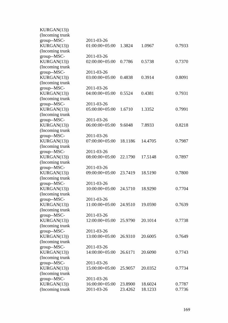
169
KURGAN(13)) (Incoming trunk group--MSC-KURGAN(13))
2011-03-26 01:00:00+05:00 1.3824 1.0967 0.7933
(Incoming trunk group--MSC-KURGAN(13))
2011-03-26 02:00:00+05:00 0.7786 0.5738 0.7370
(Incoming trunk group--MSC-KURGAN(13))
2011-03-26 03:00:00+05:00 0.4838 0.3914 0.8091
(Incoming trunk group--MSC-KURGAN(13))
2011-03-26 04:00:00+05:00 0.5524 0.4381 0.7931
(Incoming trunk group--MSC-KURGAN(13))
2011-03-26 05:00:00+05:00 1.6710 1.3352 0.7991
(Incoming trunk group--MSC-KURGAN(13))
2011-03-26 06:00:00+05:00 9.6048 7.8933 0.8218
(Incoming trunk group--MSC-KURGAN(13))
2011-03-26 07:00:00+05:00 18.1186 14.4705 0.7987
(Incoming trunk group--MSC-KURGAN(13))
2011-03-26 08:00:00+05:00 22.1790 17.5148 0.7897
(Incoming trunk group--MSC-KURGAN(13))
2011-03-26 09:00:00+05:00 23.7419 18.5190 0.7800
(Incoming trunk group--MSC-KURGAN(13))
2011-03-26 10:00:00+05:00 24.5710 18.9290 0.7704
(Incoming trunk group--MSC-KURGAN(13))
2011-03-26 11:00:00+05:00 24.9510 19.0590 0.7639
(Incoming trunk group--MSC-KURGAN(13))
2011-03-26 12:00:00+05:00 25.9790 20.1014 0.7738
(Incoming trunk group--MSC-KURGAN(13))
2011-03-26 13:00:00+05:00 26.9310 20.6005 0.7649
(Incoming trunk group--MSC-KURGAN(13))
2011-03-26 14:00:00+05:00 26.6171 20.6090 0.7743
(Incoming trunk group--MSC-KURGAN(13))
2011-03-26 15:00:00+05:00 25.9057 20.0352 0.7734
(Incoming trunk group--MSC-KURGAN(13))
2011-03-26 16:00:00+05:00 23.8900 18.6024 0.7787
(Incoming trunk 2011-03-26 23.4262 18.1233 0.7736
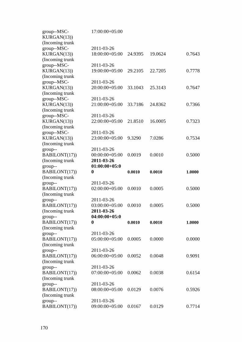
170
group--MSC-KURGAN(13))
17:00:00+05:00
(Incoming trunk group--MSC-KURGAN(13))
2011-03-26 18:00:00+05:00 24.9395 19.0624 0.7643
(Incoming trunk group--MSC-KURGAN(13))
2011-03-26 19:00:00+05:00 29.2105 22.7205 0.7778
(Incoming trunk group--MSC-KURGAN(13))
2011-03-26 20:00:00+05:00 33.1043 25.3143 0.7647
(Incoming trunk group--MSC-KURGAN(13))
2011-03-26 21:00:00+05:00 33.7186 24.8362 0.7366
(Incoming trunk group--MSC-KURGAN(13))
2011-03-26 22:00:00+05:00 21.8510 16.0005 0.7323
(Incoming trunk group--MSC-KURGAN(13))
2011-03-26 23:00:00+05:00 9.3290 7.0286 0.7534
(Incoming trunk group--BABILONT(17))
2011-03-26 00:00:00+05:00 0.0019 0.0010 0.5000
(Incoming trunk group--BABILONT(17))
2011-03-26 01:00:00+05:00 0.0010 0.0010 1.0000
(Incoming trunk group--BABILONT(17))
2011-03-26 02:00:00+05:00 0.0010 0.0005 0.5000
(Incoming trunk group--BABILONT(17))
2011-03-26 03:00:00+05:00 0.0010 0.0005 0.5000
(Incoming trunk group--BABILONT(17))
2011-03-26 04:00:00+05:00 0.0010 0.0010 1.0000
(Incoming trunk group--BABILONT(17))
2011-03-26 05:00:00+05:00 0.0005 0.0000 0.0000
(Incoming trunk group--BABILONT(17))
2011-03-26 06:00:00+05:00 0.0052 0.0048 0.9091
(Incoming trunk group--BABILONT(17))
2011-03-26 07:00:00+05:00 0.0062 0.0038 0.6154
(Incoming trunk group--BABILONT(17))
2011-03-26 08:00:00+05:00 0.0129 0.0076 0.5926
(Incoming trunk group--BABILONT(17))
2011-03-26 09:00:00+05:00 0.0167 0.0129 0.7714

171
(Incoming trunk group--BABILONT(17))
2011-03-26 10:00:00+05:00 0.0252 0.0214 0.8491
(Incoming trunk group--BABILONT(17))
2011-03-26 11:00:00+05:00 0.0176 0.0129 0.7297
(Incoming trunk group--BABILONT(17))
2011-03-26 12:00:00+05:00 0.0262 0.0162 0.6182
(Incoming trunk group--BABILONT(17))
2011-03-26 13:00:00+05:00 0.0495 0.0362 0.7308
(Incoming trunk group--BABILONT(17))
2011-03-26 14:00:00+05:00 0.1152 0.0900 0.7810
(Incoming trunk group--BABILONT(17))
2011-03-26 15:00:00+05:00 0.0686 0.0490 0.7153
(Incoming trunk group--BABILONT(17))
2011-03-26 16:00:00+05:00 0.0300 0.0224 0.7460
(Incoming trunk group--BABILONT(17))
2011-03-26 17:00:00+05:00 0.0762 0.0581 0.7625
(Incoming trunk group--BABILONT(17))
2011-03-26 18:00:00+05:00 0.3805 0.2905 0.7635
(Incoming trunk group--BABILONT(17))
2011-03-26 19:00:00+05:00 1.5024 1.1524 0.7670
(Incoming trunk group--BABILONT(17))
2011-03-26 20:00:00+05:00 2.8386 2.2424 0.7900
(Incoming trunk group--BABILONT(17))
2011-03-26 21:00:00+05:00 2.7029 2.1090 0.7803
(Incoming trunk group--BABILONT(17))
2011-03-26 22:00:00+05:00 0.2124 0.1743 0.8206
(Incoming trunk group--BABILONT(17))
2011-03-26 23:00:00+05:00 0.0076 0.0062 0.8125
(Incoming trunk group--MSC-OLD(19))
2011-03-26 00:00:00+05:00 5.4990 5.1910 0.9440
(Incoming trunk group--MSC-OLD(19))
2011-03-26 01:00:00+05:00 1.9529 1.8043 0.9239
(Incoming trunk group--MSC-
2011-03-26 02:00:00+05:00 1.0729 1.0019 0.9339

172
OLD(19)) (Incoming trunk group--MSC-OLD(19))
2011-03-26 03:00:00+05:00 0.6657 0.5614 0.8433
(Incoming trunk group--MSC-OLD(19))
2011-03-26 04:00:00+05:00 0.8129 0.7538 0.9274
(Incoming trunk group--MSC-OLD(19))
2011-03-26 05:00:00+05:00 1.8910 1.7990 0.9514
(Incoming trunk group--MSC-OLD(19))
2011-03-26 06:00:00+05:00 9.7933 9.1738 0.9367
(Incoming trunk group--MSC-OLD(19))
2011-03-26 07:00:00+05:00 23.7295 22.2086 0.9359
(Incoming trunk group--MSC-OLD(19))
2011-03-26 08:00:00+05:00 33.5724 31.3681 0.9343
(Incoming trunk group--MSC-OLD(19))
2011-03-26 09:00:00+05:00 39.2638 36.5871 0.9318
(Incoming trunk group--MSC-OLD(19))
2011-03-26 10:00:00+05:00 41.1119 38.2814 0.9312
(Incoming trunk group--MSC-OLD(19))
2011-03-26 11:00:00+05:00 40.7924 38.0605 0.9330
(Incoming trunk group--MSC-OLD(19))
2011-03-26 12:00:00+05:00 39.9519 37.2657 0.9328
(Incoming trunk group--MSC-OLD(19))
2011-03-26 13:00:00+05:00 39.6733 37.0190 0.9331
(Incoming trunk group--MSC-OLD(19))
2011-03-26 14:00:00+05:00 40.4114 37.5781 0.9299
(Incoming trunk group--MSC-OLD(19))
2011-03-26 15:00:00+05:00 40.3676 37.5995 0.9314
(Incoming trunk group--MSC-OLD(19))
2011-03-26 16:00:00+05:00 41.4200 38.5490 0.9307
(Incoming trunk group--MSC-OLD(19))
2011-03-26 17:00:00+05:00 39.6457 36.9057 0.9309
(Incoming trunk group--MSC-OLD(19))
2011-03-26 18:00:00+05:00 42.8433 39.8267 0.9296
(Incoming trunk 2011-03-26 47.6357 43.7548 0.9185
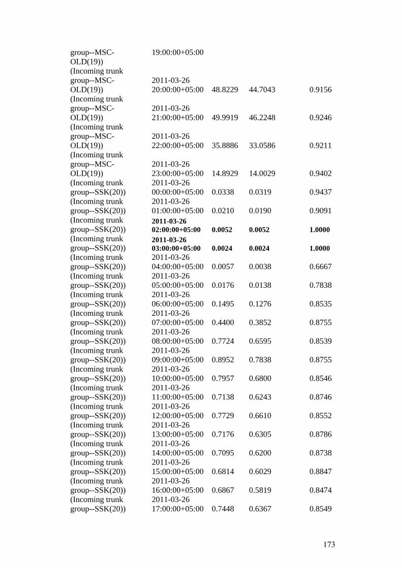
173
group--MSC-OLD(19))
19:00:00+05:00
(Incoming trunk group--MSC-OLD(19))
2011-03-26 20:00:00+05:00 48.8229 44.7043 0.9156
(Incoming trunk group--MSC-OLD(19))
2011-03-26 21:00:00+05:00 49.9919 46.2248 0.9246
(Incoming trunk group--MSC-OLD(19))
2011-03-26 22:00:00+05:00 35.8886 33.0586 0.9211
(Incoming trunk group--MSC-OLD(19))
2011-03-26 23:00:00+05:00 14.8929 14.0029 0.9402
(Incoming trunk group--SSK(20))
2011-03-26 00:00:00+05:00 0.0338 0.0319 0.9437
(Incoming trunk group--SSK(20))
2011-03-26 01:00:00+05:00 0.0210 0.0190 0.9091
(Incoming trunk group--SSK(20))
2011-03-26 02:00:00+05:00 0.0052 0.0052 1.0000
(Incoming trunk group--SSK(20))
2011-03-26 03:00:00+05:00 0.0024 0.0024 1.0000
(Incoming trunk group--SSK(20))
2011-03-26 04:00:00+05:00 0.0057 0.0038 0.6667
(Incoming trunk group--SSK(20))
2011-03-26 05:00:00+05:00 0.0176 0.0138 0.7838
(Incoming trunk group--SSK(20))
2011-03-26 06:00:00+05:00 0.1495 0.1276 0.8535
(Incoming trunk group--SSK(20))
2011-03-26 07:00:00+05:00 0.4400 0.3852 0.8755
(Incoming trunk group--SSK(20))
2011-03-26 08:00:00+05:00 0.7724 0.6595 0.8539
(Incoming trunk group--SSK(20))
2011-03-26 09:00:00+05:00 0.8952 0.7838 0.8755
(Incoming trunk group--SSK(20))
2011-03-26 10:00:00+05:00 0.7957 0.6800 0.8546
(Incoming trunk group--SSK(20))
2011-03-26 11:00:00+05:00 0.7138 0.6243 0.8746
(Incoming trunk group--SSK(20))
2011-03-26 12:00:00+05:00 0.7729 0.6610 0.8552
(Incoming trunk group--SSK(20))
2011-03-26 13:00:00+05:00 0.7176 0.6305 0.8786
(Incoming trunk group--SSK(20))
2011-03-26 14:00:00+05:00 0.7095 0.6200 0.8738
(Incoming trunk group--SSK(20))
2011-03-26 15:00:00+05:00 0.6814 0.6029 0.8847
(Incoming trunk group--SSK(20))
2011-03-26 16:00:00+05:00 0.6867 0.5819 0.8474
(Incoming trunk group--SSK(20))
2011-03-26 17:00:00+05:00 0.7448 0.6367 0.8549

174
(Incoming trunk group--SSK(20))
2011-03-26 18:00:00+05:00 0.6952 0.5943 0.8548
(Incoming trunk group--SSK(20))
2011-03-26 19:00:00+05:00 0.8000 0.7019 0.8774
(Incoming trunk group--SSK(20))
2011-03-26 20:00:00+05:00 0.6733 0.5833 0.8663
(Incoming trunk group--SSK(20))
2011-03-26 21:00:00+05:00 0.4452 0.3886 0.8727
(Incoming trunk group--SSK(20))
2011-03-26 22:00:00+05:00 0.2048 0.1810 0.8837
(Incoming trunk group--SSK(20))
2011-03-26 23:00:00+05:00 0.1000 0.0895 0.8952

175
P. The ratio between connect times and seizure times for outgoing trunk group the 21st of March 2011
Ratio:
Object Instance Start Time
Connect times /Seizure times
(Outgoing trunk group--CALLCENTER(6))
2011-03-21 00:00:00+05:00 1
(Outgoing trunk group--CALLCENTER(6))
2011-03-21 01:00:00+05:00 1
(Outgoing trunk group--CALLCENTER(6))
2011-03-21 02:00:00+05:00 1
(Outgoing trunk group--CALLCENTER(6))
2011-03-21 03:00:00+05:00 0.9921875
(Outgoing trunk group--CALLCENTER(6))
2011-03-21 04:00:00+05:00 0.992248062
(Outgoing trunk group--CALLCENTER(6))
2011-03-21 05:00:00+05:00 0.995085995
(Outgoing trunk group--CALLCENTER(6))
2011-03-21 06:00:00+05:00 0.998755445
(Outgoing trunk group--CALLCENTER(6))
2011-03-21 07:00:00+05:00 1
(Outgoing trunk group--CALLCENTER(6))
2011-03-21 08:00:00+05:00 0.99929627
(Outgoing trunk group--CALLCENTER(6))
2011-03-21 09:00:00+05:00 0.999378496
(Outgoing trunk group--CALLCENTER(6))
2011-03-21 10:00:00+05:00 0.999477261
(Outgoing trunk group--CALLCENTER(6))
2011-03-21 11:00:00+05:00 0.998709122
(Outgoing trunk group--CALLCENTER(6))
2011-03-21 12:00:00+05:00 0.999524715
(Outgoing trunk group--CALLCENTER(6))
2011-03-21 13:00:00+05:00 0.999134574
(Outgoing trunk group--CALLCENTER(6))
2011-03-21 14:00:00+05:00 0.99767658
(Outgoing trunk group--CALLCENTER(6))
2011-03-21 15:00:00+05:00 1
(Outgoing trunk group--CALLCENTER(6))
2011-03-21 16:00:00+05:00 0.998979592
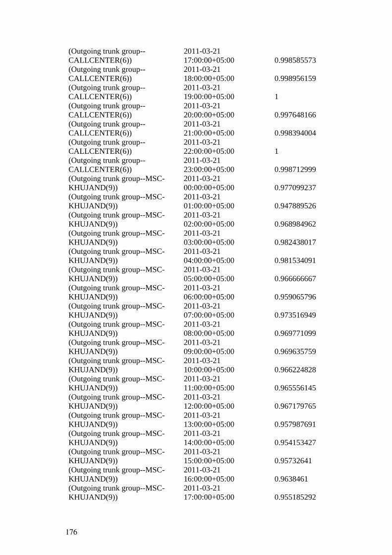
176
(Outgoing trunk group--CALLCENTER(6))
2011-03-21 17:00:00+05:00 0.998585573
(Outgoing trunk group--CALLCENTER(6))
2011-03-21 18:00:00+05:00 0.998956159
(Outgoing trunk group--CALLCENTER(6))
2011-03-21 19:00:00+05:00 1
(Outgoing trunk group--CALLCENTER(6))
2011-03-21 20:00:00+05:00 0.997648166
(Outgoing trunk group--CALLCENTER(6))
2011-03-21 21:00:00+05:00 0.998394004
(Outgoing trunk group--CALLCENTER(6))
2011-03-21 22:00:00+05:00 1
(Outgoing trunk group--CALLCENTER(6))
2011-03-21 23:00:00+05:00 0.998712999
(Outgoing trunk group--MSC-KHUJAND(9))
2011-03-21 00:00:00+05:00 0.977099237
(Outgoing trunk group--MSC-KHUJAND(9))
2011-03-21 01:00:00+05:00 0.947889526
(Outgoing trunk group--MSC-KHUJAND(9))
2011-03-21 02:00:00+05:00 0.968984962
(Outgoing trunk group--MSC-KHUJAND(9))
2011-03-21 03:00:00+05:00 0.982438017
(Outgoing trunk group--MSC-KHUJAND(9))
2011-03-21 04:00:00+05:00 0.981534091
(Outgoing trunk group--MSC-KHUJAND(9))
2011-03-21 05:00:00+05:00 0.966666667
(Outgoing trunk group--MSC-KHUJAND(9))
2011-03-21 06:00:00+05:00 0.959065796
(Outgoing trunk group--MSC-KHUJAND(9))
2011-03-21 07:00:00+05:00 0.973516949
(Outgoing trunk group--MSC-KHUJAND(9))
2011-03-21 08:00:00+05:00 0.969771099
(Outgoing trunk group--MSC-KHUJAND(9))
2011-03-21 09:00:00+05:00 0.969635759
(Outgoing trunk group--MSC-KHUJAND(9))
2011-03-21 10:00:00+05:00 0.966224828
(Outgoing trunk group--MSC-KHUJAND(9))
2011-03-21 11:00:00+05:00 0.965556145
(Outgoing trunk group--MSC-KHUJAND(9))
2011-03-21 12:00:00+05:00 0.967179765
(Outgoing trunk group--MSC-KHUJAND(9))
2011-03-21 13:00:00+05:00 0.957987691
(Outgoing trunk group--MSC-KHUJAND(9))
2011-03-21 14:00:00+05:00 0.954153427
(Outgoing trunk group--MSC-KHUJAND(9))
2011-03-21 15:00:00+05:00 0.95732641
(Outgoing trunk group--MSC-KHUJAND(9))
2011-03-21 16:00:00+05:00 0.9638461
(Outgoing trunk group--MSC-KHUJAND(9))
2011-03-21 17:00:00+05:00 0.955185292

177
(Outgoing trunk group--MSC-KHUJAND(9))
2011-03-21 18:00:00+05:00 0.962201223
(Outgoing trunk group--MSC-KHUJAND(9))
2011-03-21 19:00:00+05:00 0.943661972
(Outgoing trunk group--MSC-KHUJAND(9))
2011-03-21 20:00:00+05:00 0.941199581
(Outgoing trunk group--MSC-KHUJAND(9))
2011-03-21 21:00:00+05:00 0.952553604
(Outgoing trunk group--MSC-KHUJAND(9))
2011-03-21 22:00:00+05:00 0.967550774
(Outgoing trunk group--MSC-KHUJAND(9))
2011-03-21 23:00:00+05:00 0.97181321
(Outgoing trunk group--MSC-KURGAN(13))
2011-03-21 00:00:00+05:00 0.982256486
(Outgoing trunk group--MSC-KURGAN(13))
2011-03-21 01:00:00+05:00 0.972807018
(Outgoing trunk group--MSC-KURGAN(13))
2011-03-21 02:00:00+05:00 0.984937787
(Outgoing trunk group--MSC-KURGAN(13))
2011-03-21 03:00:00+05:00 0.96875
(Outgoing trunk group--MSC-KURGAN(13))
2011-03-21 04:00:00+05:00 0.972034716
(Outgoing trunk group--MSC-KURGAN(13))
2011-03-21 05:00:00+05:00 0.964802011
(Outgoing trunk group--MSC-KURGAN(13))
2011-03-21 06:00:00+05:00 0.966496622
(Outgoing trunk group--MSC-KURGAN(13))
2011-03-21 07:00:00+05:00 0.970637692
(Outgoing trunk group--MSC-KURGAN(13))
2011-03-21 08:00:00+05:00 0.967571174
(Outgoing trunk group--MSC-KURGAN(13))
2011-03-21 09:00:00+05:00 0.9714331
(Outgoing trunk group--MSC-KURGAN(13))
2011-03-21 10:00:00+05:00 0.969456795
(Outgoing trunk group--MSC-KURGAN(13))
2011-03-21 11:00:00+05:00 0.969788751
(Outgoing trunk group--MSC-KURGAN(13))
2011-03-21 12:00:00+05:00 0.966376565
(Outgoing trunk group--MSC-KURGAN(13))
2011-03-21 13:00:00+05:00 0.969287845
(Outgoing trunk group--MSC-KURGAN(13))
2011-03-21 14:00:00+05:00 0.964450021
(Outgoing trunk group--MSC-KURGAN(13))
2011-03-21 15:00:00+05:00 0.965
(Outgoing trunk group--MSC-KURGAN(13))
2011-03-21 16:00:00+05:00 0.966688131
(Outgoing trunk group--MSC-KURGAN(13))
2011-03-21 17:00:00+05:00 0.966225468
(Outgoing trunk group--MSC-KURGAN(13))
2011-03-21 18:00:00+05:00 0.965877158
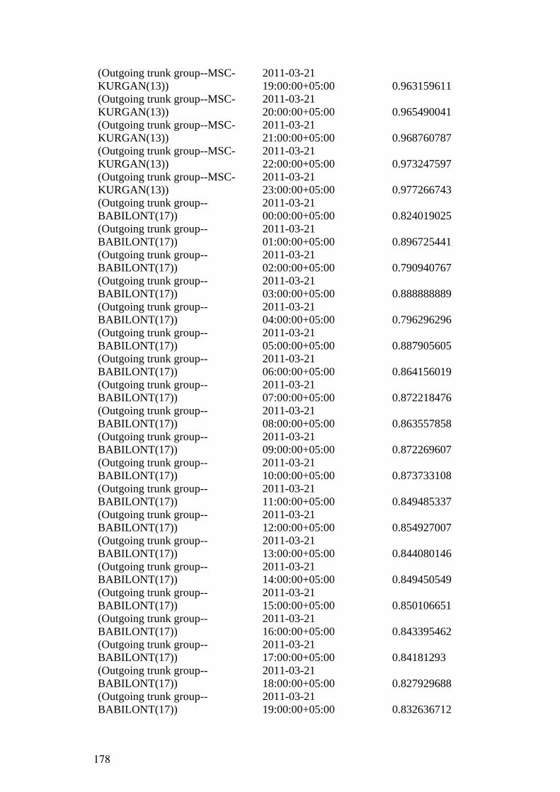
178
(Outgoing trunk group--MSC-KURGAN(13))
2011-03-21 19:00:00+05:00 0.963159611
(Outgoing trunk group--MSC-KURGAN(13))
2011-03-21 20:00:00+05:00 0.965490041
(Outgoing trunk group--MSC-KURGAN(13))
2011-03-21 21:00:00+05:00 0.968760787
(Outgoing trunk group--MSC-KURGAN(13))
2011-03-21 22:00:00+05:00 0.973247597
(Outgoing trunk group--MSC-KURGAN(13))
2011-03-21 23:00:00+05:00 0.977266743
(Outgoing trunk group--BABILONT(17))
2011-03-21 00:00:00+05:00 0.824019025
(Outgoing trunk group--BABILONT(17))
2011-03-21 01:00:00+05:00 0.896725441
(Outgoing trunk group--BABILONT(17))
2011-03-21 02:00:00+05:00 0.790940767
(Outgoing trunk group--BABILONT(17))
2011-03-21 03:00:00+05:00 0.888888889
(Outgoing trunk group--BABILONT(17))
2011-03-21 04:00:00+05:00 0.796296296
(Outgoing trunk group--BABILONT(17))
2011-03-21 05:00:00+05:00 0.887905605
(Outgoing trunk group--BABILONT(17))
2011-03-21 06:00:00+05:00 0.864156019
(Outgoing trunk group--BABILONT(17))
2011-03-21 07:00:00+05:00 0.872218476
(Outgoing trunk group--BABILONT(17))
2011-03-21 08:00:00+05:00 0.863557858
(Outgoing trunk group--BABILONT(17))
2011-03-21 09:00:00+05:00 0.872269607
(Outgoing trunk group--BABILONT(17))
2011-03-21 10:00:00+05:00 0.873733108
(Outgoing trunk group--BABILONT(17))
2011-03-21 11:00:00+05:00 0.849485337
(Outgoing trunk group--BABILONT(17))
2011-03-21 12:00:00+05:00 0.854927007
(Outgoing trunk group--BABILONT(17))
2011-03-21 13:00:00+05:00 0.844080146
(Outgoing trunk group--BABILONT(17))
2011-03-21 14:00:00+05:00 0.849450549
(Outgoing trunk group--BABILONT(17))
2011-03-21 15:00:00+05:00 0.850106651
(Outgoing trunk group--BABILONT(17))
2011-03-21 16:00:00+05:00 0.843395462
(Outgoing trunk group--BABILONT(17))
2011-03-21 17:00:00+05:00 0.84181293
(Outgoing trunk group--BABILONT(17))
2011-03-21 18:00:00+05:00 0.827929688
(Outgoing trunk group--BABILONT(17))
2011-03-21 19:00:00+05:00 0.832636712

179
(Outgoing trunk group--BABILONT(17))
2011-03-21 20:00:00+05:00 0.820656172
(Outgoing trunk group--BABILONT(17))
2011-03-21 21:00:00+05:00 0.81231593
(Outgoing trunk group--BABILONT(17))
2011-03-21 22:00:00+05:00 0.847060958
(Outgoing trunk group--BABILONT(17))
2011-03-21 23:00:00+05:00 0.850375505
(Outgoing trunk group--MSC-OLD(19))
2011-03-21 00:00:00+05:00 0.758122293
(Outgoing trunk group--MSC-OLD(19))
2011-03-21 01:00:00+05:00 0.765799082
(Outgoing trunk group--MSC-OLD(19))
2011-03-21 02:00:00+05:00 0.798313367
(Outgoing trunk group--MSC-OLD(19))
2011-03-21 03:00:00+05:00 0.769784983
(Outgoing trunk group--MSC-OLD(19))
2011-03-21 04:00:00+05:00 0.759044863
(Outgoing trunk group--MSC-OLD(19))
2011-03-21 05:00:00+05:00 0.771991029
(Outgoing trunk group--MSC-OLD(19))
2011-03-21 06:00:00+05:00 0.751628861
(Outgoing trunk group--MSC-OLD(19))
2011-03-21 07:00:00+05:00 0.745437542
(Outgoing trunk group--MSC-OLD(19))
2011-03-21 08:00:00+05:00 0.739268879
(Outgoing trunk group--MSC-OLD(19))
2011-03-21 09:00:00+05:00 0.749705962
(Outgoing trunk group--MSC-OLD(19))
2011-03-21 10:00:00+05:00 0.760486942
(Outgoing trunk group--MSC-OLD(19))
2011-03-21 11:00:00+05:00 0.769653131
(Outgoing trunk group--MSC-OLD(19))
2011-03-21 12:00:00+05:00 0.771842698
(Outgoing trunk group--MSC-OLD(19))
2011-03-21 13:00:00+05:00 0.76257368
(Outgoing trunk group--MSC-OLD(19))
2011-03-21 14:00:00+05:00 0.748391572
(Outgoing trunk group--MSC-OLD(19))
2011-03-21 15:00:00+05:00 0.736253935
(Outgoing trunk group--MSC-OLD(19))
2011-03-21 16:00:00+05:00 0.748259761
(Outgoing trunk group--MSC-OLD(19))
2011-03-21 17:00:00+05:00 0.755573228
(Outgoing trunk group--MSC-OLD(19))
2011-03-21 18:00:00+05:00 0.76161011
(Outgoing trunk group--MSC-OLD(19))
2011-03-21 19:00:00+05:00 0.779801628
(Outgoing trunk group--MSC-OLD(19))
2011-03-21 20:00:00+05:00 0.753362975

180
(Outgoing trunk group--MSC-OLD(19))
2011-03-21 21:00:00+05:00 0.705844019
(Outgoing trunk group--MSC-OLD(19))
2011-03-21 22:00:00+05:00 0.661167845
(Outgoing trunk group--MSC-OLD(19))
2011-03-21 23:00:00+05:00 0.693628112

181
Q. Configuration example of equipment data
///////////////////////////////////////////////////////////////////// // // // Example of configuration of hardware // // // // Equipment data configuration for // // MSC server in Kulyab // // // ///////////////////////////////////////////////////////////////////// //////////////////////////////////////////////// // Hardware data //////////////////////////////////////////////// // Add shelves (racks) // Add shelf where the subrack is ADD SHE: SHN=0, LT="Shelf0", ZN=1, PL=2: //Add service processing rack ADD SHE: SHN=1, LT="shelf1", PL=0; ADD SHE: SHN=2, LT="shelf2", PL=0, PT; ///////////////////////////////////////////////////////////////// // Add a basic subrack (frame) ADD FRM: FN=0, SHN=0, PN=2; // Add board to basic subrack // FRBT = Front Board Title ADD BRD: FN=0, SLN=0, LOC=FRONT, FRBT=WSCU, MN=22, ASS=1: ADD BRD: FN=0, SLN=2, LOC=FRONT, FRBT=WSCU, MN=23, ASS=3: ADD BRD: FN=0, SLN=4, LOC=FRONT, FRBT=WCCU, MN=24, ASS=5: ADD BRD: FN=0, SLN=10, LOC=FRONT, FRBT=WIFM, MN=132, ASS=11: ADD BRD: FN=0, SLN=0, LOC=BACK, BKBT=WIFM; ADD BRD: FN=0, SLN=1, LOC=BACK, BKBT=WIFM; ADD BRD: FN=0, SLN=2, LOC=BACK, BKBT=WIFM; ADD BRD: FN=0, SLN=3, LOC=BACK, BKBT=WIFM; ADD BRD: FN=0, SLN=10, LOC=BACK, BKBT=WBFI; ADD BRD: FN=0, SLN=11, LOC=BACK, BKBT=WBFI; ADD BRD: FN=0, SLN=10, LOC=BACK, BKBT=WCKL; ///////////////////////////////////////////////////////////////// // Expansion frame one and boards ADD FRM: FN=1, SHN=0, PN=3; // Boards in frame one ADD BRD: FN=1, SLN=0, LOC=FRONT, FRBT=WSCU, MN=25, ASS=1: ADD BRD: FN=1, SLN=2, LOC=FRONT, FRBT=WSCU, MN=26, ASS=3: ADD BRD: FN=1, SLN=4, LOC=FRONT, FRBT=WSCU, MN=27, ASS=5:

182
// and so on ///////////////////////////////////////////////////////////////// // FE port ADD FECFG: MN=132, IP="X.Y.Z.W", MSK="255.255.0.0", DGW="X.Y.Z.W", EA=AUTO, SO=AD-1&RFC-1; //////////////////////////////////////////////////////////////////// // E1 port data on WEPI (active and standby board) // // The format of the frames are double framed // The balance mode is balanced (120 ohm) // frame 0 ADD EPICFG: FN=0, SN=0, LM=E1, P0=DF, P1=DF, P2=DF, P3=DF, P4=DF, P5=DF, P6=DF. P7=DF, BM=BALANCED: ADD EPICFG: FN=0, SN=2, LM=E1, P0=DF, P1=DF, P2=DF, P3=DF, P4=DF, P5=DF, P6=DF. P7=DF, BM=BALANCED: // frame 1 ADD EPICFG: FN=1, SN=0, LM=E1, P0=DF, P1=DF, P2=DF, P3=DF, P4=DF, P5=DF, P6=DF. P7=DF, BM=BALANCED: ADD EPICFG: FN=1, SN=2, LM=E1, P0=DF, P1=DF, P2=DF, P3=DF, P4=DF, P5=DF, P6=DF. P7=DF, BM=BALANCED: ADD EPICFG: FN=1, SN=4, LM=E1, P0=DF, P1=DF, P2=DF, P3=DF, P4=DF, P5=DF, P6=DF. P7=DF, BM=BALANCED: // and so on

183
R. Configuration example for local office data
////////////////////////////////////////////////////////// // // // Example of configuration of hardware // // // // Hardware configuration of MSC server // // in Kulyab // // // ////////////////////////////////////////////////////////// ////////////////////////////////////////////////////////// // Local office data ////////////////////////////////////////////////////////// // Local signaling point // The office is a MSC local office that is in a national signaling network and in a national // reserved network. The first search network is national and the 2nd, 3rd and 4th is national // reserved. // The national point code (NPC) is xxxxxx and the national reserved point code is xxxxxx // The structure of the national code (NNS) and national reserved code (NR2S) is 14 bits and 14 bits // The transmission delay is set to 0. It doesn't serve as a STP (it is a GMSC and VMSC) // The location is either 0050 or 0051 (in hexadecimals). The country code is 992 and // the packet network access code is 918 // There is no CBF (BTVM) and CFNR (NTVM) voice mailbox number. // The core network ID is xxxxx SET OFI: OFN="MSCServer_Kulyab", LOT=LOCMSC, IN=no, IN2=no, NN=yes, NN2=yes, SN1=NAT, SN2=NATB, SN3=NAT, SN4=NATB, IPC="000000", IP2C="000000" NPC="00138D", NP2C="00138F", INS=SP14, IN2S=SP14, NNS=SP14, NN2S=SP14, TADT=0. STP=no, LAC="0050", LNC="992", GAC="918", BTVM=no, NTVM=no, CNID=65535, QAAL2CAPABILITY=CSI, MULTAREAMSFLAG=no, ACLKSP=0, RCTRAP=0, TDMSPFAXDT=yes, SPRED=no: // Local mobile office information // The mobile country code is 436 and the mobile network code is 04 SET INOFFMSC: MSCN="992918xxxxxx", VLRN="992918xxxxxx", MCC="436", MNC="04", LOCALNUM="50",

184
INNATIONPFX=810, NATIONPFX=8, LACCIUNIQUE=true; // VLR information // LOCUPDT is the implicit IMSI detach timer in minutes. Default value is 120. This value // should be greater than the periodic subscriber location update in the BSC // a small value saves wireless resources because it decrease the amount of // time the subscriber is paged ADD VLRCFG: MAXUSR=200000, MCC="436", CC="992", LOCUPDT="245"; // and so on

185
S. Average call duration calculated for the measurement period 23rd of February to 25th of March 20011 Table 48, Table 49, Table 50, and Table 51 gives the call duration for the
actual period.
Table 48: Average call duration from 23rd of February to 1st of March 2011
Start Time
23rd of February
24th of February
25th of February
26th of February
27th of February
28th of February
1st of March
(Hour) (s) (s) (s) (s) (s) (s) (s) 0 22.9 24.9 24.4 23.3 24.0 22.8 23.2 1 20.4 22.3 23.7 21.6 24.5 24.1 23.7 2 19.4 22.4 17.9 19.8 24.9 23.9 26.8 3 16.8 16.9 15.3 16.8 26.0 16.6 25.8 4 15.5 17.3 15.2 17.6 19.5 17.1 20.3 5 13.1 14.0 13.4 12.6 13.8 12.2 13.7 6 18.0 17.2 15.7 16.1 17.3 15.7 18.9 7 24.5 23.8 23.4 22.9 22.8 22.6 24.5 8 27.7 27.6 26.0 25.7 25.0 26.5 27.4 9 28.5 27.4 25.6 25.6 24.5 26.2 27.7 10 28.3 26.8 24.7 24.7 24.4 25.3 27.1 11 28.4 26.6 24.5 23.9 24.3 24.5 25.8 12 27.4 24.6 23.2 23.0 24.4 23.7 24.3 13 27.7 24.3 23.1 23.0 24.1 24.2 24.4 14 28.8 24.9 24.5 23.4 24.3 24.0 25.1 15 28.4 24.8 24.4 24.0 25.1 24.1 24.8 16 27.9 25.4 24.3 24.5 25.9 24.3 24.8 17 30.1 26.9 25.7 25.5 27.1 25.0 25.7 18 31.3 27.7 27.3 27.1 29.7 26.4 27.7 19 34.9 32.0 31.4 32.0 33.9 30.8 33.9 20 36.0 32.1 30.7 30.9 33.2 30.5 32.9 21 32.3 29.1 27.1 28.5 30.6 27.0 29.2 22 27.0 25.5 24.1 24.4 25.9 22.9 25.3 23 25.8 25.2 22.9 23.3 23.9 22.7 22.5 All day (s): 621.1 589.7 558.6 560.3 599.0 563.3 605.5 All day (min.): 10.4 9.8 9.3 9.3 10.0 9.4 10.1

186
Table 49: Average call duration from the 4th of March to 10th of March 2011
Start Time 4th of March
5th of March
6th of March
7th of March
8th of March
9th of March
10th of March
(Hour) (s) (s) (s) (s) (s) (s) (s)
0 22.7 21.5 21.9 22.0 24.1 22.9 21.5 1 21.9 19.2 20.8 21.0 21.7 23.4 24.0 2 20.2 17.9 19.2 25.3 25.1 21.2 25.8 3 18.3 18.5 18.0 25.0 27.5 22.0 18.7 4 17.8 15.2 16.3 20.8 24.1 23.2 16.5 5 14.6 11.1 13.4 14.0 18.8 16.4 14.9 6 16.9 16.3 16.6 17.8 25.0 18.4 18.9 7 24.9 24.2 23.9 24.5 34.7 26.2 25.1 8 27.5 27.1 25.2 27.0 33.9 27.4 27.4 9 27.4 26.8 24.7 26.3 32.9 28.3 27.6 10 26.4 26.3 25.2 26.0 31.7 27.9 27.0 11 25.7 25.9 24.8 26.3 30.6 27.6 26.1 12 23.7 24.3 24.4 25.9 29.7 26.9 25.1 13 23.5 23.9 24.6 26.7 30.1 25.9 25.1 14 25.1 25.1 25.6 26.6 29.8 26.4 25.9 15 25.3 25.6 25.3 26.7 30.0 27.3 26.2 16 25.9 25.9 25.8 27.9 30.1 26.5 26.7 17 26.8 27.2 27.9 29.2 31.1 27.7 26.4 18 29.6 29.0 29.0 30.8 32.5 29.7 28.1 19 34.6 34.2 35.2 39.1 39.6 34.5 33.4 20 32.8 33.9 34.5 38.7 41.5 34.4 33.9 21 28.2 30.6 30.6 34.2 36.5 29.8 30.5 22 24.4 25.9 24.0 27.4 29.1 25.5 25.1 23 22.9 24.0 22.1 24.1 24.4 23.9 23.5
All day (s) 586.9 579.5 579.0 633.3 714.4 623.5 603.3 All day (min.) 9.8 9.7 9.7 10.6 11.9 10.4 10.1

187
Table 50: Average call duration from the 11th of March to 19th of March 2011
Start Time
11th of March
12th of March
13th of March
14th of March
15th of March
18th of March
19th of March
(Hour) (s) (s) (s) (s) (s) (s) (s)
0 22.603 24.314 24.370 24.117 25.602 24.122 25.116
1 21.918 25.105 22.754 22.951 27.642 24.168 25.995
2 19.237 25.571 20.503 21.282 22.658 18.783 20.363
3 18.448 24.796 19.318 22.094 25.577 24.433 26.045
4 17.179 18.549 15.861 17.341 20.462 17.466 20.809
5 13.497 15.186 14.313 12.117 12.479 15.010 15.303
6 19.127 20.212 19.910 20.768 20.781 21.964 23.200
7 25.451 25.447 26.067 26.123 25.382 27.205 28.034
8 27.124 26.905 25.373 27.350 26.545 26.629 27.130
9 27.408 26.765 25.896 27.921 27.212 27.006 26.784
10 26.773 26.384 25.553 27.623 27.130 26.639 27.502
11 25.698 26.020 25.374 27.487 26.440 26.339 27.036
12 24.831 25.138 25.133 25.648 26.051 24.881 26.790
13 25.035 24.966 25.439 25.822 26.375 25.404 27.327
14 25.848 26.256 26.578 26.314 26.453 26.341 27.978
15 26.535 25.904 26.391 26.239 26.640 26.528 28.716
16 26.605 26.494 26.519 27.406 26.921 27.689 29.091
17 27.106 27.126 27.931 28.119 28.693 28.752 29.133
18 28.339 28.227 28.964 28.724 29.815 29.619 29.740
19 33.071 34.575 34.416 34.837 37.621 37.382 37.357
20 34.021 34.154 35.251 35.348 36.038 39.251 37.965
21 31.188 32.478 31.332 33.212 30.178 34.614 35.374
22 25.610 25.726 26.710 26.927 26.010 29.186 27.894
23 24.167 25.569 25.997 25.164 25.379 28.154 25.057
All day (s) 596.820 621.867 605.957 620.934 634.085 637.563 655.739
All day (min.) 9.947 10.364 10.099 10.349 10.568 10.626 10.929
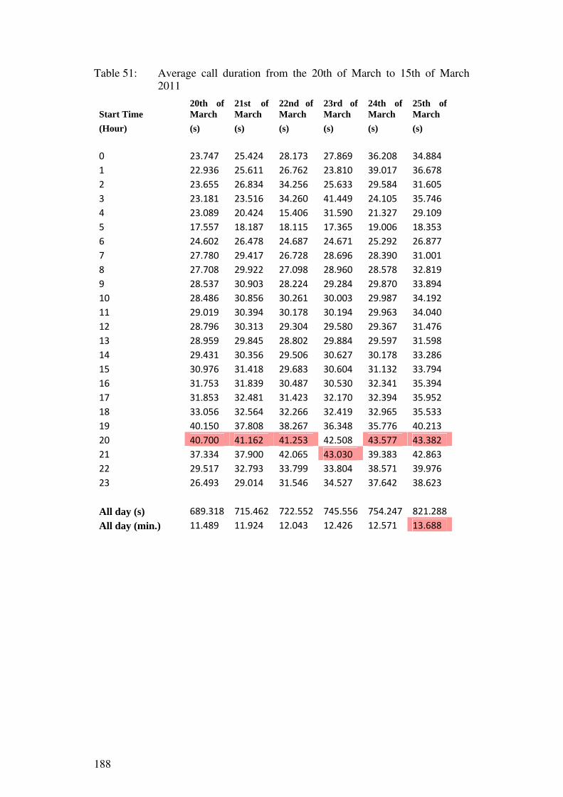
188
Table 51: Average call duration from the 20th of March to 15th of March 2011
Start Time 20th of March
21st of March
22nd of March
23rd of March
24th of March
25th of March
(Hour) (s) (s) (s) (s) (s) (s)
0 23.747 25.424 28.173 27.869 36.208 34.884 1 22.936 25.611 26.762 23.810 39.017 36.678 2 23.655 26.834 34.256 25.633 29.584 31.605 3 23.181 23.516 34.260 41.449 24.105 35.746 4 23.089 20.424 15.406 31.590 21.327 29.109 5 17.557 18.187 18.115 17.365 19.006 18.353 6 24.602 26.478 24.687 24.671 25.292 26.877 7 27.780 29.417 26.728 28.696 28.390 31.001 8 27.708 29.922 27.098 28.960 28.578 32.819 9 28.537 30.903 28.224 29.284 29.870 33.894 10 28.486 30.856 30.261 30.003 29.987 34.192 11 29.019 30.394 30.178 30.194 29.963 34.040 12 28.796 30.313 29.304 29.580 29.367 31.476 13 28.959 29.845 28.802 29.884 29.597 31.598 14 29.431 30.356 29.506 30.627 30.178 33.286 15 30.976 31.418 29.683 30.604 31.132 33.794 16 31.753 31.839 30.487 30.530 32.341 35.394 17 31.853 32.481 31.423 32.170 32.394 35.952 18 33.056 32.564 32.266 32.419 32.965 35.533 19 40.150 37.808 38.267 36.348 35.776 40.213 20 40.700 41.162 41.253 42.508 43.577 43.382 21 37.334 37.900 42.065 43.030 39.383 42.863 22 29.517 32.793 33.799 33.804 38.571 39.976 23 26.493 29.014 31.546 34.527 37.642 38.623
All day (s) 689.318 715.462 722.552 745.556 754.247 821.288 All day (min.) 11.489 11.924 12.043 12.426 12.571 13.688
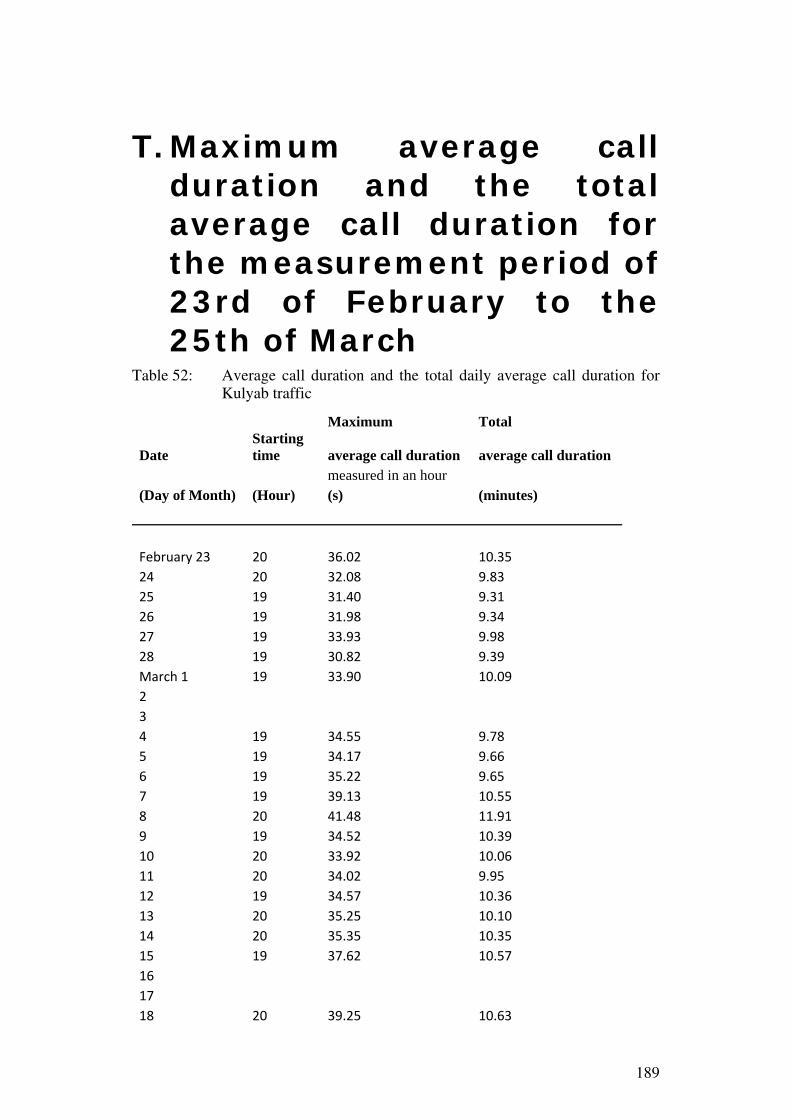
189
T. Maximum average call duration and the total average call duration for the measurement period of 23rd of February to the 25th of March
Table 52: Average call duration and the total daily average call duration for Kulyab traffic
Maximum Total
Date Starting time average call duration average call duration
measured in an hour (Day of Month) (Hour) (s) (minutes)
February 23 20 36.02 10.35 24 20 32.08 9.83 25 19 31.40 9.31 26 19 31.98 9.34 27 19 33.93 9.98 28 19 30.82 9.39 March 1 19 33.90 10.09 2 3 4 19 34.55 9.78 5 19 34.17 9.66 6 19 35.22 9.65 7 19 39.13 10.55 8 20 41.48 11.91 9 19 34.52 10.39 10 20 33.92 10.06 11 20 34.02 9.95 12 19 34.57 10.36 13 20 35.25 10.10 14 20 35.35 10.35 15 19 37.62 10.57 16 17 18 20 39.25 10.63

190
19 20 37.96 10.93 20 20 40.70 11.49 21 20 41.16 11.92 22 20 41.25 12.04 23 21 43.03 12.43 24 20 43.58 12.57 25 20 43.38 13.69

www.kth.se
TRITA-ICT-EX-2011:140