trading volume and serial correlation ... - dash.harvard.edu · the harvard community has made this...

Trading Volume and Serial Correlation in Stock Returns

(Article begins on next page)

The Harvard community has made this article openly available.

Please share how this access benefits you. Your story matters.

Citation Campbell, John Y., Sanford J. Grossman, and Jiang Wang. 1993.Trading volume and serial correlation in stock returns. QuarterlyJournal of Economics 108, no. 4: 905-939.

Published Version doi:10.2307/2118454

Accessed July 15, 2018 3:19:18 PM EDT

Citable Link http://nrs.harvard.edu/urn-3:HUL.InstRepos:3128710

Terms of Use This article was downloaded from Harvard University's DASHrepository, and is made available under the terms and conditionsapplicable to Other Posted Material, as set forth athttp://nrs.harvard.edu/urn-3:HUL.InstRepos:dash.current.terms-of-use#LAA

http://osc.hul.harvard.edu/dash/open-access-feedback?handle=1/3128710&title=Trading+Volume+and+Serial+Correlation+in+Stock+Returns&community=1/1&collection=1/2&owningCollection1/2&harvardAuthors=null,null,db2e31e3f14d93f85769d95abf793eaa&department=Economics

http://dx.doi.org/10.2307/2118454

http://nrs.harvard.edu/urn-3:HUL.InstRepos:dash.current.terms-of-use#LAA

http://nrs.harvard.edu/urn-3:HUL.InstRepos:dash.current.terms-of-use#LAA

TRADING VOLUME AND SERIAL CORRELATION INSTOCK RETURNS*

JOHN Y. CAMPBELLSANFORD J . GROSSMAN

JIANG WANG

This paper investigates the relationship between aggregate stock markettrading volume and the serial correlation of daily stock returns. For both stockindexes and individual large stocks, the first-order daily return autocorrelationtends to decline with volume. The paper explains this phenomenon using a model inwhich risk-averse "market makers" accommodate buying or selling pressure from"liquidity" or "noninformational" traders. Changing expected stock returns re-ward market makers for playing this role. The model implies that a stock pricedecline on a high-volume day is more likely than a stock price decline on alow-volume day to be associated with an increase in the expected stock return.

I. INTRODUCTION

There is now considerable evidence that the expected returnon the aggregate stock market varies through time. One interpreta-tion of this fact is that it results from the interaction betweendifferent groups of investors. Suppose that some investors,"liquidity" or more generally "noninformational" traders, desireto sell stock for exogenous reasons. Other investors Eire risk-averseutility maximizers; they are willing to accommodate the selhngpressure, but they demand a reward in the form of a lower stockprice and a higher expected stock return. If these investorsaccommodate the fluctuations in noninformational traders' de-mand for stock, then they can be thought of as "market makers" inthe sense of Grossman and Miller [1988], even though they mayhold positions for relatively long periods of time and may not bespeciedists on the exchange.

It is hard to test this view of the stock market using data onstock returns alone, because very diflferent models can have similar

*We thank J. Harold Mulherin and Mason Gerety for providing data on dsiilyNYSE volume, G. William Schwert for providing daily stock return data, MartinLettau for correcting an error in the theoretical model, Ludger Hentschel for ableresearch assistance throughout this project, £ind four anonymous referees andseminar participeints at Princeton University and the 1991 NBER SummerInstitute for helpful comments. Campbell acknowledges financial support from theNational Science Foundation and the Sloan Foundation. Wang acknowledgessupport from the Nanyang Technological University Career Development AssistantProfessorship at the Sloan School of Management.

1. See also Campbell and Kyle [1993]; De Long, Shleifer, Summers, andWaldmann [1989,1990]; Shiller [1984]; Wang [1993a, 1993b]; and others.

© 1993 by the President and Fellows of Harvard College and the Massachusetts Institute ofTechnology.The Quarterly Journal of Economics, November 1993

906 QUARTERLY JOURNAL OF ECONOMICS

implications for the time-series behavior of returns. In this paperwe use data on stock market trading volume to help solve thisidentification problem. The simple intuition underljdng our work isas follows. Suppose that one observes a fall in stock prices. Thiscould be due to public information that has caused all investors toreduce their valuation of the stock market, or it could be due toexogenous selling pressure by noninformational traders. In theformer case, there is no reason why the expected return on thestock market should have changed. In the latter case, marketmakers buying stock will require a higher expected return, so therewill tend to be price increases on subsequent days. The two casescan be distinguished by looking at trading volume. If publicinformation has arrived, there is no reason to expect a high volumeof trade, whereas selling pressure by noninformational tradersmust reveal itself in unusual volume. Thus, the model withheterogeneous investors suggests that price changes accompaniedby high volume will tend to be reversed; this will be less true ofprice changes on days with low volume.

Shifts in the demand for stock by noninformational traderscan occur at low frequencies or at high frequencies. Daily tradingvolume is a signal for high frequency shifts in demand. Changes indemand that occur slowly through time are heirder to detect usingvolume data because there are trends in volume associated withother phenomena such as the deregulation of commissions and thegrowth of institutional trading. We therefore focus on daily tradingvolume and the serial correlation of daily returns on stock indexesand individual stocks. Daily index autocorrelations are predomi-nantly positive [Conrad and Kaul, 1988; Lo and MacKinlay, 1988],but our theory predicts that they will be less positive on high-volume days.

The literature on stock market trading volume is extensive,but is mostly concerned with the relationship between volume andthe volatility of stock returns. Numerous papers have documentedthe fact that high stock market volume is associated with volatilereturns; October 19, 1987, is only the best known example of apervasive phenomenon.^ It has also been noted that volume tendsto be higher when stock prices are increasing than when prices arefalling.

2. See Gallant, Rossi, and Tauchen [1992]; Harris [1987]; Jain and Joh [1988];Jones, Kaul, and Lipson [1991]; Mulherin and Gerety [1989]; Tauchen and Pitts[1983]; ajid the survey in Karpoff [1987]. Lamoureux and Lastrapes [1990] arguethat serial correlation in volume accounts for the serial correlation in volatilitywhich is often described using ARCH models.

VOLUME AND SERIAL CORRELATION IN STOCK RETURNS 907

In contrast, there is almost no work relating the serialcorrelation of stock returns to the level of volume. One exception isMorse [1980], who studies the serial correlation of returns inhigh-volume periods for 50 individual securities. He finds thathigh-volume periods tend to have positively autocorrelated re-turns, but he does not compare high-volume with low-volumeperiods.^ Several recent papers study serial correlation in relationto volatility: LeBaron [1992a] and Sentana and Wadhwani [1992],for example, show that the autocorrelations of daily stock returnschange with the variance of returns. Below, we compare the effectsof volume and volatility on stock return autocorrelations.

The organization of our paper is £is follows. In Section II weconduct a preliminary exploration of the relation between volume,volatility, and the serial correlation of stock returns. In Section IIIwe present a theoretical model of stock returns and tradingvolume. In Section IV we show that the model can generateautocorrelation patterns similar to those found in the actual data.We use both approximate anal)i;ical methods and numerical simu-lation methods to make this point. Section V concludes.

II. VOLUME, VOLATILITY, AND SERIAL CORRELATION: APRELIMINARY EXPLORATION

A. Measurement Issues

The main return series used in this paper is the daily return ona value-weighted index of stocks traded on the New York StockExchange and American Stock Exchange, measured by the Centerfor Research in Security Prices (CRSP) at the University ofChicago over the period 7/3/62 through 12/30/88. Results withdaily data over this period are likely to be dominated by a fewobservations around the stock market crash of October 19, 1987.For this reason, the main sample period we use in this paper is ashorter period running from 7/3/62 through 9/30/87 (1962-1987for short, or SEimple A). We break this period into two subsamples:7/3/62 through 12/31/74 (1962-1974 for short, or sample B),which is the first half of the shorter sample and which excludes the

3. Some other papers have come to our attention since the first draft of thispaper was written. Duffee [1992] studies the relation between serial correlation andtrading volume in aggregate monthly data, while LeBaron [1992b] uses nonparamet-ric methods to characterize the aggregate daily relation more accurately. Conrad,Hameed, and Niden [1992] study the relation between individual stocks' returnautocorrelations and the trading volume in those stocks.


period of flexible commissions on the New York Stock Exchange;and 1/2/75 through 9/30/87 (1975-1987 for short, or sample C),which is the remainder of the shorter sample period. Finally, weuse the complete data set through the end of 1988 in order to seewhether the extreme movements of price and volume in late 1987strengthen or weaken the results we obtain in our other samples.We call this long sample 1962-1988 for short, or sample D.

We also study the behavior of some other stock return series.For the period before CRSP daily data begin, Schwert [1990] hasconstructed daily returns on an index comparable to the Standardand Poors 500. We use this series over the period 1/2/26-6/29/62.The behavior of large stocks is of particular interest, since mea-sured returns on these stocks are unlikely to be affected bynonsynchronous trading. The Dow Jones Industrial Average is thebest known large stock price index, and so we study its changesover the period 1962-1988. Individual stock returns also provideuseful evidence robust to nonos3Tichronous trading, so we studythe returns on 32 large stocks that were traded throughout the1962-1988 period and were among the 100 largest stocks on both7/2/62 and 12/30/88.^

Stock market trading volume data were kindly provided to usby J. Harold Mulherin and Mason S. Gerety. These researcherscollected data from The Wall Street Journal and Barron's on thenumber of shares traded daily on the New York Stock Exchangefrom 1900 through 1988. They also collected data on the number ofshares outstanding on the New York Stock Exchange. For adetailed description of their data, see Mulherin and Gerety [1989].

The ratio of the number of shares traded to the number ofshares outstanding is known as turnover, or sometimes as relativevolume. Turnover is used as the volume measure in most previousstudies (for example, Jain and Joh [1988] and Mulherin and Gerety[1989]). Since the number of shares outstanding and the number ofshares traded have both grown steadily over time, the use ofturnover helps to reduce the low-frequency variation in the series.It does not eliminate it completely, however, as can be seen fromthe plot of the series presented in Figure I. Turnover has anupward trend in the late 1960s and in the period between the

4. The 32 stocks are American Home Products, AT&T, Amoco, Caterpillar,Chevron, Coca Cola, Commonwealth Edison, Dow Chemical, Du Pont, EastmanKodak, Exxon, Ford, GTE, General Electric, General Motors, ITT, Imperial Oil,IBM, Merck, 3M, Mobil, Pacific Gas and Electric, Pfizer, Procter and Gamble, RJRNabisco, Royal Dutch Petroleum, SCE, Sears Roebuck, Southern, Texaco, USX, andWestinghouse.


Raw Turnover

o 60

FIGURE ILevel of Stock Market Turnover, 1960-1988

elimination of fixed commissions in 1975 and the stock marketcrash of 1987. The growth of turnover in the 1980s may be due inpart to technological innovations that have lowered transactionscosts. In addition, the variance of turnover seems to increase withits level during the 1980s.

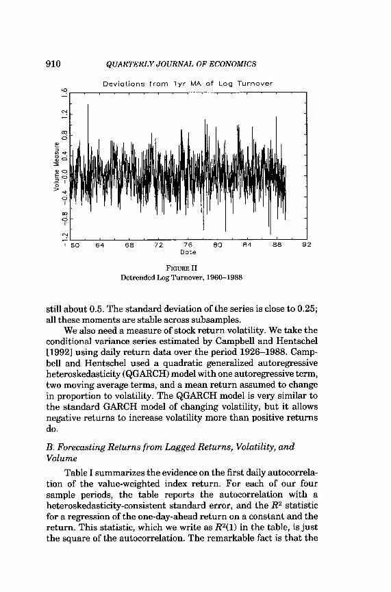
In our empirical work, we want to work with stationary timeseries. When we relate our empirical results to our theoreticalmodel, we want to measure trading volume relative to the capacityof the market to absorb volume. For both these reasons we wish toremove the low-frequency variations from the level and variance ofthe turnover series. To remove low-frequency variations from thevariance, we measure turnover in logs rather thEm in absoluteunits. To detrend the log turnover series, we subtract a one-yeEU-backward moving average of log turnover. This gives a triangularmoving average of turnover growth rates, similar to the geometri-cally declining average of turnover growth rates used by Schwert[1989] to explain stock return volatility. We explore some alterna-tive detrending procedures below.

Our detrended volume measure is plotted in Figure II. Thefigure shows no trends in mean or variEmce, but it does showconsiderable persistence. The first daily autocorrelation of de-trended volume is about 0.7, and the fifth daily autocorrelation is


Deviat ions f r a m l y r MA af Log Turnover

I 50 6 4

FIGURE IIDetrended Log Turnover, 1960-1988

still about 0.5. The stEmdard deviation of the series is close to 0.25;all these moments are stable across subsamples.

We also need a measure of stock return volatility. We take theconditional variance series estimated by Campbell and Hentschel[1992] using daily return data over the period 1926-1988. Camp-bell and Hentschel used a quadratic generalized autoregressiveheteroskedasticity (QGARCH) model with one autoregressive term,two moving average terms, and a mean return assumed to changein proportion to volatility. The QGARCH model is very similar tothe standard GARCH model of changing volatility, but it Eillowsnegative returns to increase volatility more than positive returnsdo.

B. Forecasting Returns from Lagged Returns, Volatility, andVolume

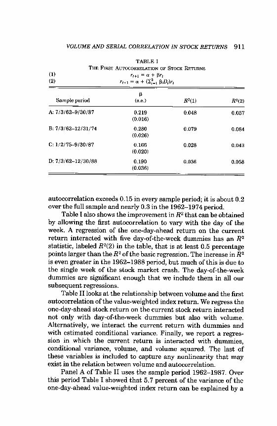
Table I summarizes the evidence on the first daily autocorrela-tion of the vEilue-weighted index return. For each of our foursample periods, the table reports the autocorrelation with aheteroskedasticity-consistent standard error, and the R^ statisticfor a regression of the one-day-ahead return on a constant Emd thereturn. This statistic, which we write as RHD in the table, is justthe square of the autocorrelation. The remarkable fact is that the


TABLE ITHE FIRST AUTOCORRELATION OF STOCK RETURNS

(1) n+i = a + pr,\^) ri+i = a + (Z:,

Sample period

A:7/3/62-9/30/87

B:7/3/62-12/31/74

C:1/2/75-9/30/87

D:7/3/62-12/30/88

(s.e.)

0.219(0.016)

0.280(0.026)

0.166(0.020)

0.190(0.036)

RHD

0.048

0.079

0.028

0.036

RH2)

0.057

0.084

0.043

0.058

autocorrelation exceeds 0.15 in every sample period; it is about 0.2over the full sample and neEirly 0.3 in the 1962-1974 period.

Table I also shows the improvement in R^ that can be obtainedby allowing the first autocorrelation to vary with the day of theweek. A regression of the one-day-ahead return on the currentreturn interacted with five day-of-the-week dummies has an R^statistic, labeled RH2) in the table, that is at least 0.5 percentagepoints larger than the R^ of the basic regression. The increase in R^is even greater in the 1962-1988 period, but much of this is due tothe single week of the stock market crash. The day-of-the-weekdummies are significant enough that we include them in all oursubsequent regressions.

Table II looks at the relationship between volume Emd the firstautocorrelation of the value-weighted index return. We regress theone-day-ahead stock return on the current stock return interactednot only with day-of-the-week dummies but also with volume.Alternatively, we interact the current return with dummies andwith estimated conditional variance. Finally, we report a regres-sion in which the current return is interacted with dummies,conditional variance, volume, and volume squared. The last ofthese variables is included to capture any nonlinearity that mayexist in the relation between volume and autocorrelation.

Panel A of Table II uses the sample period 1962-1987. Overthis period Table I showed that 5.7 percent of the variance of theone-day-ahead value-weighted index return can be explained by a


TABLE IIVOLUME, VOLATILITY, AND THE FIRST AUTOCORRELATION

n+i = a + (2f,i PiDi + yiVt + yiVf + 73(1000af))r,

Sample periodand specification

71(s.e.)

72(s.e.)

73(s.e.)

A: 7/3/62-9/30/87Volume

Volatility

Volume and volatility

B:7/3/62-12/31/74Volume

Volatility

Volume £ind volatility

C:1/2/75-9/30/87Volume

Volatility


D:7/3/62-12/30/88Volume

Volatility


-0.328(0.060)

-0.427(0.077)

-0.445(0.114)

-0.546(0.112)

-0.214(0.073)

-0.212(0.110)

-0.169(0.080)

-0.290(0.148)

0.265(0.140)

0.511(0.259)

0.056(0.179)

0.173(0.116)

-0.047(0.241)

0.055(0.248)

-0.058(0.283)

0.112(0.290)

-0.879(0.392)

-0.661(0.391)

-0.068(0.106)

-0.025(0.105)

0.065

0.057

0.066

0.095

0.084

0.097

0.046

0.045

0.047

0.062

0.059

0.064

regression on current return interacted with day-of-the-weekdummies. The first row of panel A shows that this R^ statistic CEmbe increased to 6.5 percentage points by interacting the regressorwith dummies and detrended trading volume. The coefficient onthe product of volume £md the stock return is —0.33 with aheteroskedasticity-consistent standard error of 0.06. This is eco-nomically as well as statistically significEmt. The standard devia-tion of detrended volume is about 0.25. Thus, as volume movesfrom two stEmdard deviations below the mean to two standarddeviations above, the first-order autocorrelation of the stock returnis reduced by about 0.3.


These strong results for volume are not matched by ourvolatility measure. Wben volume is excluded from tbe regression,volatility enters negatively, but it is statistically and economicallyinsignificant. Wben volume and volume squared appear in tberegression, volatility enters positively but is again insignificant.Tbe quadratic term on volume is positive and not quite significantat tbe 5 percent level. Tbus, in panel A there is only weak evidencefor any specification more complicated tban tbe linear volumeregression reported in the second row.

In panels B and C of Table II, we break tbe 1962-1987 periodinto subsamples 1962-1974 and 1975-1987. The strongest resultscome from the earlier subsample 1962-1974. In tbis period tbeaverage first-order autocorrelation of tbe stock return is almost0.3, and a regression of tbe one-day-ahead return on the currentreturn interacted with day-of-the-week dummies gives an R^statistic of 8.4 percent. This can be increased by more than apercentage point by taking account of a linear relationsbip betweenthe autocorrelation and trading volume. Once again volatility andquadratic volume terms add little. In the later subsample, 1975-1987, the first-order autocorrelation is much smaller on average.Volume raises the regression R^ from 4.3 percent only to 4.6percent, although tbe linear volume term is still statisticallysignificant with a ^statistic of 2.9. In this period there is a strongernegative relationship between volatility and autocorrelation, al-though volume is still slightly superior to volatility when botb areincluded in tbe regression.

Finally, in panel D of Table II we ask wbether the addition ofthe stock market crash period to the sample weakens or reinforcesour results. It turns out that the most recent data weaken the effectof volume on the first-order autocorrelation of returns. Even in the1962-1988 period, however, volume remains significant at the 5percent level. We note also that the 1962-1988 period is the onlyone for which day-of-the-week dummies make a major difierence tothe results. When these dummies are excluded, the volume effectbecomes mucb stronger in tbe 1962-1988 period than in the1962-1987 period. This is because the stock price reversals of theweek of October 19, 1987, are captured by day-of-tbe-week dum-mies wben these are included, or by volume wben dummies areomitted.

Table III bas exactly tbe same structure as Table I, but nowtbe dependent variable is tbe two-day-abead stock return so tbetable describes tbe second-order autocorrelation of the return. The


THE SECOND

(1)(2)

Sample period

A: 7/3/62-9/30/87

B: 7/3/62-12/31/74

C: 1/2/75-9/30/87

D:7/3/62-12/30/88

TABLE IIIAUTOCORRELATION

O+2 = a + P

P(s.e.)

0.016(0.017)

0.017(0.030)

0.013(0.019)

-0.011(0.039)

OF STOCK RETURNS

RHD

0.000

0.000

0.000

0.000

RH2)

0.004

0.009

0.002

0.012

average second-order autocorrelation is small and statisticallyinsignificant in every sample period. Even when day-of-the-weekdummies are interacted with the current return, the R^ statistic ofthe regression is less than 1.5 percent.

Table IV, which has the same structure as Table II, showssome evidence for volume effects on the second autocorrelation.However, the evidence is much weaker thEm that for volume effectson the first autocorrelation. Over the 1962-1987 sample period(panel A) we find that volume enters the regression significantlyonly when it is included in quadratic form. The linear coefficient is-0.23 with a standard error of 0.08, while the quadratic coefficientis 0.55 with a standard error of 0.15. These coefficients imply thatthe second-order autocorrelation falls with volume until volumereaches 0.2, about two-thirds of a standard deviation above itsmean. At higher levels of volume the positive quadratic termdominates, and the autocorrelation starts to increase again. Look-ing at subsamples in panels B and C, we find that the evidence forvolume effects on the second autocorrelation comes entirely fromthe 1962-1974 period. Finally, in panel D we see that the additionof the stock market crash period leads to stronger evidence for avolume effect on the second autocorrelation.

One might ask whether higher-order autocorrelations alsochange with trading volume. As a crude way to answer thisquestion without having to look at each autocorrelation individu-


TABLE IVVOLUME, VOLATILITY, AND THE SECOND AUTOCORRELATION

n+2 = a + all PiA + 7lV, + 72Vf + •Y3(1000a, ))r,


A: 7/3/62-9/30/87Volume

Volatility


B: 7/3/62-12/31/74Volume

Volatility


C:1/2/75-9/30/87Volume

Volatility


D:7/3/62-12/30/88Volume

Volatility


71(s.e.)

-0.028(0.060)

-0.233(0.079)

-0.186(0.115)

-0.390(0.113)

0.074(0.069)

-0.015(0.109)

-0.178(0.089)

-0.024(0.087)

72(s.e.)

0.550(0.146)

1.149(0.345)

0.138(0.175)

-0.241(0.119)

73(s.e.)

0.086(0.276)

0.071(0.276)

-0.012(0.338)

-0.039(0.326)

0.613(0.391)

0.500(0.400)

0.007(0.105)

0.072(0.102)

0.004

0.004

0.008

0.011

0.009

0.021

0.003

0.003

0.004

0.016

0.011

0.019

ally, we have run regressions of stock returns on moving averagesof past stock returns and on moving averEiges of past stock returnsinteracted with trading volume. Regressions of this sort (where thelags in the moving averages run from 1 to 5 or from 2 to 6) yieldresults similar to those reported in Tables II Emd IV, withsomewhat reduced statistical significance. This suggests that themain volume effects are in the first couple of autocorrelations, butthat there are at least no offsetting effects in higher autocorrela-tions out to lags 5 or 6.


VOLUME,

rt+i = a 4

Sample period andspecification

A:7/3/62-9/30/87Detrended volume

Total volume

Detrended andtrend volume

B: 7/3/62-12/31/74Detrended volume

Total volume


C:1/2/75-9/30/87Detrended volume

Total volume


D: 7/3/62-12/30/88Detrended volume

Total volume


TABLEVOLATILITY, AND THE

VFIRST AUTOCORRELATION:

ALTERNATIVE VOLUME MEASURES

• a l , p,A- + 7iV< + •)

71(s.e.)

-0.328(0.060)

-0.313(0.061)

-0.445(0.114)

-0.417(0.108)

-0.214(0.073)

-0.218(0.073)

-0.169(0.080)

-0.134(0.066)

i^MAV, + 73(V,

72(s.e.)

-0.090(0.037)

0.292(0.141)

-0.090(0.046)

-0.065(0.059)

+ MAV,))ri

73(s.e.)

-0.156(0.028)

-0.227(0.081)

-0.132(0.040)

-0.091(0.050)

R^

0.065

0.064

0.066

0.095

0.087

0.097

0.046

0.047

0.047

0.062

0.063

0.064

C. Alternative Volume and Volatility Measures

So far we have worked exclusively with detrended volume. It isnatural to ask whether similar results could be achieved withoutdetrending. To answer this, in Table V we run similar regressionsto those in Table II, but using total volume instead of detrendedvolume. We also run regressions including both the detrendedseries and the trend. The general pattern is that detrended volumehas superior explanatory power to total volume, Eilthough this isnot true in 1975-1987. When both detrended and trend volume are


included, the coefficient on detrended volume is always negativeEmd significEmt, whereas the coefficient on the trend switches signfrom positive in 1962-1974 to negative in 1975-1987.

In an earlier version of this paper, we also used an unobservedcomponents model to stochastically detrend volume. The resultingseries was much less persistent than the detrended series usedhere, having a positive first-order autocorrelation and than a seriesof negative higher-order autocorrelations. The stochastically de-trended volume series gave results similar to but systematicallyweaker than those in Table 11. This can be interpreted in terms ofour theoretical expectation that the serial correlation of stockreturns declines when volume increases relative to the ability ofmarket makers to absorb volume. A one-year backward movingaverage of past volume, which reacts sluggishly to changes involume, seems to be a better measure of market making capacitythan an estimated random walk component from an unobservedcomponents model, which reacts very quickly to changes in volume.

To check the robustness of this finding, we have also triedmeasuring volume as the deviations of log turnover from three-month Emd five-year backward moving averages. Both these alter-native moving average measures gave results similar to thosereported in Table II. Thus, it seems to be importEmt to measurevolume relative to a slowly adjusting trend, but the exact details oftrend construction are not crucial.

The results reported above also use a single measure ofvolatility, the fitted value from a QGARCH model. The choice ofthis particular model in the GARCH class is not critical since allmodels in this class give very similar fitted variances. Nelson[1992] shows that high-frequency data can be used to estimatevariance very precisely, even when variance is changing throughtime and the true model for variance is unknown.

It could be objected, however, that estimated conditionalvolatility cannot compete equally with trading volume becauseeach day's conditional variance uses information only through the

5. LeBaron [1992b] builds on the work of this paper to explore the relationbetween autocorrelation and high-frequency volume movements more thoroughly.

6. Grossman and Miller [1988] model the long-run determination of market-making capacity and show that in steady state the constant negative autocorrelationof stock price changes is determined by the cost of maintaining a market presenceand the risk aversion of market makers. We believe that meirket-making capacityadjusts slowly to the steady state, and this is consistent with our empirical results.For simplicity, our theoretical model assumes that market-making capacity is fixed;it is a short-run counterpart to Grossman and Miller's long-run model.


TABLE VITHE FIRST AUTOCORRELATION OF STOCK RETURNS: ALTERNATIVE SAMPLE PERIODS

(1) n+i = a + Pr,(2) r,+i = a + (S,t

Sample period

E;1/2/26-6/29/62

F: 1/2/26-12/30/39

G:1/2/40-12/31/49

H:1/3/50-6/29/62

I: 1/2/26-9/30/87

P(s.e.)

0.039(0.023)

0.015(0.029)

0.112(0.034)

0.130(0.036)

0.073(0.019)

RHD

0.002

0.000

0.012

0.017

0.005

RH2)

0.005

0.004

0.018

0.037

0.008

previous day. A simple way to respond to this is to add the currentsquared return to the regression, since in any GARCH model thesquared return is the innovation in conditional variance. When wedo this, we find that the current squared return sometimes enterssignificantly but does not have any important effect on theestimated volume effect. To save space, we do not report results forthis specification.

D. Evidence from Earlier Periods

As a further check on the robustness of our results, in TablesVI and VII we look at Schwert's [1989] daily stock indexreturn over the period from 1926. The tables use five differentsamples: the full pre-1962 data set 1/2/26-6/29/62 (sample E);decadal subsamples 1/2/26-12/30/39, 1/2/40-12/31/49, and1/3/50-6/29/62 (samples F, G, and H, respectively); and a longsample splicing together Schwert's series with the CRSP value-weighted index over the period 1/2/26-9/30/87 (sample I).''

Table VI shows that the average first autocorrelation of stockreturns has varied considerably over the decades. In the 1930s itwas very small at 0.015, but it increased to above 0.1 in the 1940sand 1950s. Table VII shows that the effect of volume on autocorre-

7. Sample I is long enough that adding the stock market crash period hasvery little efFect on the results, so to save space we do not report results for1/2/26-12/30/88.


TABLE VIIVOLUME, VOLATILITY, AND THE FIRST AUTOCORRELATION:

ALTERNATIVE SAMPLE PERIODSr,+i = a + (2f=i P,A + 7iV, + 7,

Sample period andspecification

E:1/2/26-6/29/62Volume

Volatility


F:1/2/26-12/30/39Volume

Volatility


G:1/2/40-12/31/49Volume

Volatility


H:1/3/50-6/29/62Volume

Volatility


I: 1/2/26-9/30/87Volume

Volatility

Volume emd volatility

71(s.e.)

0.053(0.045)

-0.114(0.039)

-0.038(0.053)

-0.131(0.047)

-0.097(0.061)

-0.104(0.062)

-0.174(0.099)

-0.152(0.094)

-0.085(0.043)

-0.119(0.039)

72(S.e.)

0.064(0.051)

0.079(0.058)

0.046(0.064)

0.216(0.175)

0.050(0.049)

73(s.e.)

0.006

-0.002(0.041)

0.009(0.043)

0.027(0.044)

0.042(0.046)

-0.173(0.114)

-0.130(0.145)

-0.420(0.199)

-0.492(0.244)

-0.029(0.040)

-0.014(0.041)

0.005

0.004

0.004

0.007

0.021

0.021

0.022

0.042

0.044

0.046

0.011

0.009

0.011


THE

Sample period

A:7/3/62-9/30/87

B:7/3/62-12/31/74

C: 1/2/75-9/30/87

D: 7/3/62-12/30/88

TABLE VIIIFIRST AUTOCORRELATION OF STOCK RETURNS:

THE DOW JONES INDUSTRIAL AVERAGE

(1) rt+i = a + pr,(2) r,+i = a + (2f=i &iDi)rt

P(s.e.)

0.141(0.016)

0.210(0.026)

0.087(0.019)

0.106(0.045)

RHl)

0.020

0.044

0.008

0.011

RH2^

0.027

0.046

0.023

0.034

lation has always been negative, although in many sample periodsit is statistically significant only when squared volume and volatil-ity are also included in the regression.^ Volatility is statisticallysignificant only in the period 1950-1962.

E. Nonsynchronous Trading

All the empirical results so far have used the return on avalue-weighted stock index. It could be objected that the serialcorrelation of the index return is mismeasured because the indi-vidual stocks in the index are not all traded exactly at the close. Inprinciple, nonsynchronous trading can lead to spurious positiveautocorrelation in an index return, although Lo and MacKinlay[1990] have shown that this effect is very small unless stocks fail totrade for implausibly long periods of time.

As one way to respond to this objection, in Tables VIII and IXwe repeat our basic regressions using price changes of the DowJones Industrial Average. Although this series omits dividends,this has only a minimal effect on daily autocorrelations. Nonsyn-chronous trading should also have only a trivial effect on thebehavior of the Dow Jones. The average autocorrelation of the DowJones is much smaller than the average autocorrelation of the

8. An anonymous referee has objected that we report results with squaredvolume only because they are statistically significant. We note, however, that wereported the same squared volume regressions in the first version of this paperwhich did not look at the older data.


TABLEVOLUME, VOLATILITY, AND THE

THE:

r,+i = a + C


A: 7/3/62-9/30/87Volume

Volatility


B:7/3/62-12/31/74Volume

Volatility


C: 1/2/75-9/30/87Volume

Volatility


D: 7/3/62-12/30/88Volume

Volatility

Volume Eind volatility

IXFIRST AUTOCORRELATION:

Dow JONES INDUSTRIAL AVERAGE

Ef=i P A + 7iVi

71(s.e.)

-0.257(0.061)

-0.358(0.074)

-0.359(0.116)

-0.450(0.112)

-0.157(0.073)

-0.177(0.102)

-0.127(0.094)

-0.251(0.159)

+ 72V, + 73(1001

72(s.e.)

0.278(0.147)

0.498(0.276)

0.138(0.174)

0.103(0.142)

73(s.e.)

-0.142(0.263)

0.080(0.268)

-0.128(0.304)

0.023(0.308)

-1.138(0.380)

-1.036 .(0.372)

0.037(0.134)

0.081(0.132)

R''

0.032

0.027

0.033

0.053

0.046

0.055

0.025

0.026

0.027

0.037

0.034

0.039

vEilue-weighted portfolio, only one-half as large in some periods.However, there is still a highly significant estimated effect ofvolume on the autocorrelation.

Another way to respond to the nonsynchronous trading con-cern is to use data on individual stock returns. Nonsynchronoustrading creates spurious positive autocorrelation in an indexreturn because today's market return is measured contemporane-ously for those stocks that trade today, but only with a lag fornontraded stocks. However, nonsynchronous trading has only atrivial effect on measured individual stock return autocorrelations[Lo and MacKinlay, 1990]. Even when one uses individual stock


TABLE XVOLUME AND THE FIRST AUTOCORRELATION: INDIVIDUAL STOCK RETURNS

Equal-weighted index regression:

Pooled regression:

r , . ,+ i + ap + ( 2 f = i P P , A + ypV,)rj,,, j=l,...,32

Individual stock regressions:

n.t+i = «j + (Sf=i hiDi + yjVt)rj,t, 7 = 1, . . . , 327 = (1/32) SfJi yj, i, = (1/32) if^^t.j

Sample period

A: 7/3/62-9/30/87

B: 7/3/62-12/31/74

C: 1/2/75-9/30/87

D: 7/3/62-12/30/88

(s.e.)

-0.311(0.064)

-0.469(0.127)

-0.160(0.074)

-0.173(0.116)

(s.e.)

-0.093(0.028)

-0.125(0.049)

-0.062(0.034)

-0.121(0.083)

7(# < 0)

-0.092(31)

-0.122(30)

-0.059(25)

-0.108(31)

(# < -1.64)

-1.368(12)

-1.104(11)

-0.719(6)

-1.087(5)

returns, aggregate volume is probably a better variable thanindividual volume because idiosyncratic buying or selling pressuredoes not create systematic risk for market makers. Accordingly, wecombine individual stock returns with the single aggregate volumeseries.

Table X summarizes results for 32 large stocks that weretraded throughout the period 1962-1988 and were among the 100largest at both the beginning and end of the period. The firstcolumn of the table reports the volume effect on the autocorrela-tion of an equally weighted index of these stocks. The index is verysimilar to the Dow Jones, having an almost identical first autocor-relation and a correlation with the Dow Jones of about 0.95. Notsurprisingly, therefore, the effect of volume on the index autocorre-lation is similar to the effect reported in Table IX. The secondcolumn of Table X shows the volume effect on the correlation ofeach stock return with its own first lag, where the individualreturns are stacked together in a single pooled regression. Thestandard error is corrected for heteroskedasticity and for thecontemporaneous correlation of individual stock returns, using themethod of White [1984]. The volume effect on the own autocorrela-


tion of each stock return is smaller than the volume effect on theindex return, but the statistical significance of the effect is notmuch reduced.

The third column of Table X shows the average effect ofvolume on the first autocorrelation across 32 separate OLS regres-sions, one for each individual stock. Not surprisingly the cross-sectional average effect is close to the effect in the pooled regres-sion. The number of negative individual coefficients is also reported;at least 25 of these coefficients are negative in every sample period.Finally, the fourth column of Table X shows the cross-sectionalaverage ^-statistic for the effect of volume on the autocorrelation,and the number of individual ^statistics that are less than -1.64(the 5 percent level for a one-tailed test, or the 10 percent level for atwo-tailed test). The cross-sectional average ^-statistic is less than- 1 in every period except 1975-1987, and as many as a third of theindividual ^statistics are less than -1.64.

We interpret these results as strong evidence that nonsynchro-nous trading is not solely responsible for the phenomena we havedescribed.

III. VOLUME AND STOCK RETURNS: A THEORETICAL MODEL

In this section we present a model of noninformational tradingthat can account for the empirical relationship between tradingvolume and the serial correlation of stock returns. Several authors,including Campbell and Kyle [1993], De Long, Shleifer, Summers,and Waldmann [1989, 1990], Grossman and Miller [1988], andShiller [1984], have developed models in which expected stockreturns vary through time as some investors accommodate theshifting stock demands of other investors. But none of theseauthors explicitly work out the implications of their models fortrading volume.

Most previous work has modeled noninformational trading asan exogenous process. De Long, Shleifer, Summers, and Waldmann[1989,1990] derive noninformational trading from shifting misper-ceptions of future stock payoffs. Here we derive noninformationaltrading from shifts in the risk aversion of some traders. We do thisbecause we find it natural to relate changing demands to chang-ing tastes,^ but the basic intuition of our model carries through

9. For simplicity, we treat shifts in investors' risk aversion as exogenous. Moregenerally, investors' attitudes toward risk may depend on wealth and other statevariables. This can lead them to follow dynamic hedging strategies even when theyface a constant investment opportunity set [Grossman and Zhou, 1992].


regardless of how noninformational trading is introduced. Anysuch trading will give the same qualitative relation betweenvolume and the serial correlation of returns.

We consider an economy in which there exist two assets: arisk-free asset and a risky asset ("stock"). We Eissume thatinnovations in the stock price are driven by three random vari-ables: (i) the innovation to the current dividend, (ii) the innovationto information about future dividends, and (iii) the innovation tothe time-v£uying risk aversion of a subset of investors. Shock (i)causes the payoff to the stock to be stochastic so that a premium isdemanded by investors for holding it. Shock (iii) generates changesin the market's aggregate risk aversion, which cause the expectedreturn on the stock to vary. Shock (ii) is in the model so that pricesand dividends do not fully reveal the state of the economy andvolume provides additional information.

The properties of our model can be understood as follows. If alarge subset of investors becomes more risk averse, and the rest ofthe economy does not change its attitudes toward risk, then themeirginal investor is more risk averse, and in equilibrium, theexpected return from holding the stock must rise to compensatethe marginal investor for bearing the risk. Simultaneously, risk isreallocated from those people who become more risk averse to therest of the market. The reallocation is observed as a rise in tradingvolume. Note that the rise in expected future returns is broughtabout by a fall in the current stock price that causes a negativecurrent return. Therefore, a large trading volume will be associatedwith a relatively large negative autocorrelation of returns.

A. The Economy

Our model further specifies the economy as follows. Therisk-free asset, which is in elastic supply, guarantees a rate ofreturn R = 1 + r with r > 0. We assume that there is a fixed supplyof stock shares per capita, which is normalized to 1. Shares aretraded in a competitive market. Each sheire pays a dividend inperiod t oi Dt = D + D . D > 0 is the mean dividend, while Dt isthe zero-mean stochastic component of the dividend. (We usesimilar notational conventions for other variables below.) Dtfollows the process:

Dt = aoDt-i + UDP 0 < ao < 1.

We assume that the innovation UD,t is i.i.d. with normal distribu-tion UD,t ~ I


There are two types of investors in the economy, type A andtype B. Both types of investors have constant absolute riskaversion. The type A investors' risk aversion parameter is aconstant a, while the type B investors' risk aversion parameter isbt, which may change over time. Let w be the fraction of type Ainvestors.

Each period, investors solve the following problem:

(1) max Et[-exp (-^Wi^i)], ^ = a,6,,

subject to

Wt^, = WtR+ XtiPt^i + Dt^,

where Wt is wealth, Xt is the holding of the risky asset, and Pt is theex dividend share price of the stock, all measured at time t. Et is theexpectation operator conditioned on investors' information set J <at time t.

The set J < contains the stock price P, and the dividend D(. Italso contains a signal, St, which all investors receive at time t aboutthe future dividend shock

For simplicity, we assume that S and eo t+i are jointly i.i.d. normal,,ci), andSt'

B. The Equilibrium Price of the Risky Asset

Let F((the "cum-dividend fundamental value" of the stock) bethe present value of the expected future cash fiow from a share ofthe stock, including today's dividend, discounted at the risk-freerate. It is easy to show that

( 3 ) - - - - - - - ""r R — OLQ R —

and that the innovation variance of F,, of, is given by

In the case that investors are risk neutral. Ft - Dt gives theequilibrium ex-dividend price of the stock. When investors are riskaverse, however, the equilibrium price will depend on the riskaversion of the market.

Define a variable Z, that can be interpreted as the risk aversion


of the marginal investor in the market:

abf

' (1 - a))a + (o6('

Let Zt = Z + Zt. We assume that Z follows an AR(1) process:

(6) Zt = CLzZt-x + Uzp 0 < az < 1.

We also assume that uzf is independent of other shocks and is i.i.d.normal: uz<t ~ .>'(0,o-|). This assumption allows Zt, and thus bt, tobe negative. This could be avoided, however, if we replaced theexponential utility assumption (1) by the assumption that inves-tors have mean-variance preferences; that is, they maximize theobjective function E^t+\ - ^ var(W<+i/2. All the results in thepaper would follow, and we could restrict the Zt process to bebounded away from zero.

Finally, we assume that af < af = {R - az)2/4af. Thisassumption is used to derive an equilibrium price function wherethe price of the stock is a decreasing function of the aggregate riskaversion Z,.

THEOREM 1. For the economy defined above, there exists anequilibrium price of the stock that has the following form:

(7) Pt = Ft-Dt + ipo

where pz_= -{{R - az)/2o|)[l - v/l - (o§/a|2)] and(1 - az)pz;Z/r < 0.

Proof of Theorem 1. See Appendix A.

C Excess Stock Returns and Trading Volume

The excess return per share on the stock realized at time t + 1is written as Qt+i = Pt+i + Dt+i - RPt. Given the equilibrium price,the expected excess return anticipated by investors in period t,denoted by e , is

(8) et

where CTQ = var [Q(+i | J^ J. Then, we have

(9) Qt^i = et + K{e,+i - £,[e,+i]) + (F,+i - .B,[F,+i]),

where K = PZ/<J'Q. Equation (8) states that the unexpected excessstock return per share has two components: innovations in ex-pected excess returns per share and innovations in expected future

VOL UME AND SERIAL CORRELATION IN STOCK RETURNS 927

cash fiows per share. Given the return process (9), the serialcorrelation in returns can be easily calculated:

Qt, Qt^i] i ^ .Q L - az (TQ

Clearly, PQ,,Q, J is positive if a^ > 1/R and is negative if az < 1/R.Let Z° and Xf be, respectively, the optimal stock holdings of type Aand type B investors. The solution of the optimization problem (1)yields

(11)

varChanges in investors' preferences relative to one another

generate trading. X" (and X*) change as Zt changes:

(12) X° - XU = aia)(Zt - Zt-y).

Trading volume is then

(13) Vt = a)|X° - Z°_i| = (Wa)|Z, - Z,_i|.

Given the Zt process, mean trading volume is V = E{Vt\ — (2a>CTz)/). Equation (13) completes the solution of the model for

the joint behavior of volume and stock returns.

rv. IMPLICATIONS OF THE MODEL FOR VOLUME AND SERIALCORRELATION

Investors in the economy have perfect information about thecurrent level of Z . They can use Zt to predict future excess returnsas shown by equation (7). When Zt is high, the type B investors arehighly risk averse and less willing to hold the stock. The price of thestock has to adjust to increase the expected future excess return sothat the type A investors are induced to hold more of the stock.

We, as econometricians, do not directly observe Zt or St. Weobserve only realized excess returns and trading volume, i" How-ever, these variables do provide some information about the

10. We could actually use a finer information set containing dividends, prices,and volume. This would improve our inferences about Zt. For simplicity, however,we use only excess returns and volume in this paper.


current level of Z and can help predict future returns. A low returndue to a drop in the price could be caused either by an increase in Ztor by a low realization oi St, i.e., bad news about future cash flow.However, changes in Z, will generate trading among investors,while public news about future cash flows vdll not. Therefore, lowreturns accompanied by high trading volume are more likely due toincreases in Zt while those accompginied by low trading volume aremore likely due to low realizations of Sf In the case of an increasein Zt, the expected excess return for next period will be high, whilefor the case of low St, it will not. Thus, the autocorrelation of thestock return should decline with trading volume.

A. Analytical Results

In this subsection we use analytical methods to develop thisintuition more formally. In the next subsection we use simulationmethods to a similar end.

We want to calculate the predictable component in the excessreturn based on the current return and volume: E[Qt+i\Qt,Vt] =a^ElZt I Qt,Vtl The following theorem holds.

THEOREM 2. Under the assumptions we have made about thestructure of the economy and the distribution of shocks, wehave

(14)

A quadratic approximation to equation (14) is

(15) E[Qt^, I Qt] = (4,Q - HvVf)Qt,

where {Q<^v) > 0.

Proof of Theorem 2. See Appendix B.

In order to understemd the results in Theorem 2, first considerthe case where volume Vi = 0. In this case, there is no change inthe investors' relative risk aversion (i.e., Zt has remained thesame). Hence, there should be no change in the expected excessreturn from the previous period. The realized excess return approx-imates the expected excess return in the previous period. Thus,EQ

Now consider the case where volume is not zero. This impliesthat a risk preference shock has occurred. Note that if Q( = 0 (i.e.,there were no unusual date t returns), then E[Qt+i \ Qt= O,VJ = 0,


independent of the value of Vt. Although volume implies that Zt isdifferent from Zt-i, it does not reveal the direction of the change. IfQt is negative, however, we can infer that Z< is more likely to haveincreased than decreased, and thus the expected value of .Z( is high.Given a negative Qt, the higher is Vt, the higher is the implied valueofZ,.

We can re-express equation (15) in a form that looks moresimilar to the regression equations used in the previous section:

(16) E[Qt^, I Qt,Vt] = (4.0 -

where ^i is positive while the sign of ^o is ambiguous. (SeeAppendix B.)

In Theorem 2 we only consider how current volume in additionto the current return can help in predicting future returns. Inprinciple, we could use the whole history of returns and volume toforecast future returns. Let J^f = {Q.,,V^: T < ) be the informationset that contains the history of excess returns and volume up toand including period t. The forecasting problem faced by aneconometrician is to calculate the conditional expectation:E[Qt+i IJ^*] =CTQE[Z« |J^(*]. This is a nonlinear filtering problem forwhich there is no simple solution. We could calculate the condi-tional expectation iteratively: having calculated the expectationconditional on the return and volume in the current period, wecould calculate the expectation conditional on the return andvolume in the current and the previous period, and so on [Wang,1993a]. This process would reveal higher-order dynamic relationsbetween return and volume, which could be related to empiricalwork like that of Brock, Lakonishok, and LeBaron [1992]. How-ever, this is outside the scope of the current paper.

Theorem 2 provides some justification for the exploratoryregressions we reported in the empirical section of the paper. Thetheorem states that aggregate risk aversion (and hence the ex-pected stock return) is related to the lagged stock return and to thelagged return interacted with volume. The coefficient on thevolume-weighted lagged return should be negative, as we found inthe data. Note that there is some slippage between the theoreticalvariables in our model and the variables measured in our empiricalwork. The model generates predictions about the level of turnover£ind the serial correlation of returns per share, while our empiricalwork concerns the detrended log of turnover and the serialcorrelation of log returns per dollar invested.


B. Simulation Results

Although the analysis of the previous subsection makes ourbasic point, that volume and serial correlation should be negativelyrelated in our heterogeneous-agent model, it is not clear whetherthis effect is quantitatively important for plausible parametervalues. In this subsection we run some simple simulations toaddress this question. The model of Section III, with normaldriving processes, is straightforward to simulate because it is alinear model conditional on investors' information. It only becomesnonhnear when we condition on the smaller information setcontaining volume and returns alone. The key question is how tocalibrate the parameters of the model.

We begin by describing the riskless and risky assets in theeconomy. We set the riskless interest rate R equal to 1.01 at anannual rate, or 1.00004 at a daily rate assuming that there are 250trading days in a year. We set the autoregressive parameter for thestock dividend, ao, equal to one. This makes the dividend a randomwalk. In daily data any plausible dividend process will have a^ veryclose to one, and the model is simplified by setting it equal to one.Next we normalize the stock price so that it equals one when sdl thestochastic terms equal zero, and set stochastic terms to zero at thebeginning of our simulations. This normalization means that theaverage stock price should not be too far from one during oursimulation periods, although the stock price process has a unit rootso there is no fixed mean. The normalization makes absolute pricevariability close to percentage price variability, and it ensures thatthe coefficient of absolute risk aversion and the coefficient ofrelative risk aversion are similar if initial riskless asset holdings aresmall."

The next step is to pick a plausible value for the innovationvariance of of the stock's fundamental value Ff We choose CT|. =(0.01)2, so that the standard deviation of the daily stock return (inthe absence of shifting risk aversion) is 1 percent. This is a littlehigher than the average in postwar data. Equation (4) gives theimplications of this choice for the variances of the dividend signalSt and the contemporaneous dividend innovation e,. If there is nodividend signal, then CT| = 0, and the implied variance of thedividend innovation e is a^ = (R - D^apR^. If all dividend

11. Note that riskless asset holdings of the agents are not identified by themodel. With exponential utility, these holdings do not affect demand for the riskyasset.

VOL UME AND SERIAL CORRELATION IN STOCK RETURNS 931

information is received one day in advance, then a^ = 0, and (T| =(R - D^af. The simulation results are only trivially affected byvarying the relative importance of the dividend signal and thecontemporaneous dividend innovation.

We now turn to the specification of the two groups of investors.Suppose initiEilly that both groups have the same average riskaversion coefficient. Then this coefficient can be identified from thestock demand equation (11). When all investors have constant riskaversion a, then (11) implies that a = E[Qt+i]/var [Qt+i]. If stockprice equals fundamental value, then var [Qt+i] = ajr = (0.01)^.Setting a = 3 gives a reasonable value for E[Qt+i] of 0.0003, or 7.5percent at an annual rate. This procedure for estimating averagerisk aversion is a variant of that proposed by Friend and Blume[1975].

Next we consider w, the proportion of market-making agents.Given the Z, process, this parameter plays two roles. First, inequation (13) the trading volume generated by a given shift in Zt isproportional to (a/a. Second, in equation (5) the mapping betweenZt and the risk aversion of hquidity traders bt is determined by co.When CO is small, Zt moves almost one-for-one with bt; when w islarge, on the other hand, large shifts in 6, result in smaller changes

It turns out that if we set a = 3, then we must also pick a verysmall value of co, 0.0005. Figure I shows that turnover is typically0.5 percent or less. In exploratory simulations with larger values ofCO, the VEiriation in Zt required to explain the effect of volume onautocorrelation generates too much trading volume when market-makers have risk aversion a = 3. We can, however, increase thefraction of market-makers if we also make market-makers morerisk averse, since volume is determined by the ratio co/a. We obtainalmost identicEil simulation results, for example, if we set co = 0.005and a = 30, while keeping the mean of Z( equal to 3 to match themean stock return.

The trickiest part of the calibration is to specify the dynamicsof the Zt process. We would like to pick a process that generatesrealistic stock price behavior. Equation (6) gives the price innova-tion variance as/ j |a | + cjf. Unfortunately, the coefficientj^z is itselfa function of cr| and the other parameters of the model. When CT| =0, however. Appendix A shows that pz = PziO) = -o^KR - "z)-The coefficient pziO) is the value of j^z that obtains when Z isdeterministic. As a simple way to calibrate the model, we define acoefficient \ equal to the standard deviation of price innovations


caused by randomness in Z divided by the standard deviation ofinnovations in fundsunental value, evaluated i

(17) \ = = ^ —Op K —

Solving this equation for of, we find that

(18) (4 = \HR •

This equation can be substituted into the condition that CT| < af ,which guarantees a real solution for the coefficient pz- We can thenrestate that condition in the simple form K < 0.5. Thus, onlylimited extra stock price variability can be generated by shiftingrisk aversion.

In preliminary simulations, we varied X over the permissiblerange from 0 to 0.5, while at the same time varying the persistenceparameter az over its permissible range from 0 to 1. We found astrong negative relation between trading volume and the firstreturn autocorrelation only for \ values above about 0.2, and azvalues below about 0.5. With smaller values of X, shifting riskaversion did not have a sufficient effect on stock price behavior tobe readily detectable, even with very large numbers of observa-tions. With larger values of az, price changes caused by changingrisk aversion are largely permanent so trading volume does notstrongly signal that price movements will be reversed. For the finalsimulations reported below, we picked \ = 0.25 and az = 0, 0.25,and 0.5.

Once we have chosen parameter values, we can solve for theprice coefficients po and pz. The final step is to choose an initialdividend Do to meet our requirement that the initial price equalone. We then draw normal innovations with the appropriatevariances and create artificial data on stock prices and tradingvolume. We create series that have 3000 observations (roughly thenumber of observations in our 1962-1974 and 1975-1987 sub-samples) after discarding the first 100 observations.

Illustrative simulation results are reported in Table XI. Thetable shows regression results for a standard AR(1) return modeland for our model interacting the return with trading volume. Allparameters are fixed as described above, except for the parameteraz which describes the persistence of shifts in risk aversion. Thisparameter is 0 in panel A of Table XI, 0.25 in panel B, and 0.5 inpanel C. In panel A we find a strong effect of volume on the firstautocorrelation of returns. The ^-statistic on volume is 3.67, and


TABLE XISIMULATIONS OF VOLUME AND THE FIRST AUTOCORRELATION

Specification

A: a = 0AR(1)

Volume

B: a = 0.25AR(1)

Volume

C: a = 0.5AR(1)

Volume

P(.t)

-0.082(4.50)0.009

(0.307)

-0.036(2.03)0.051

(0.165)

-0.005(0.261)0.024

(0.840)

71it)

-16.23(3.67)

-25.12(3.45)

-14.07(1.26)

0.007

0.011

0.001

0.005

0.000

0.001

the addition of volume to the regression increases the R ^ statisticby more than 50 percent (although of course the R ^ remains verylow in absolute terms). The coefficient on volume is -16.2, whilethe standard deviation of volume (not shown in the table) is 0.0036.Thus, when volume moves from two standard deviations below themean to two standard deviations above, the autocorrelation of thestock return falls by 0.23, an economically significant amount.

As the persistence of risk aversion increases, the relationbetween volume and autocorrelation weakens. Results in panel Bare only slightly weaker than those in panel A, but in panel C thecoefficient on volume is statistically insignificaint Eilthough thepoint estimate is still negative. Even with az = 0.5, the half-life of ashift in risk aversion is only one trading day, so it is clear that riskaversion shifts must be highly transitory for our model to fit thedata.

A related problem for our model is that the parameter valuesin Table XI imply extreme movements in average risk aversion Zt.The simulation reported in panel A has a sample average for Z< of3.42, close to the population value of 3. The sample standarddeviation is 25.2, with a minimum of -89 and a maximum of 88.Given that market-makers are assumed to be a very small fraction


of the market, the implied movements of liquidity traders' riskaversion bt are almost equal to those of Z<. (As noted above, a largervalue of CO would imply larger movements in bt relative to Zt,worsening this problem.) As az increases, the movements in Z, areslightly dampened, but they remain extreme even when az = 0.5.The sample average Zt in panel C is 2.80, with a standard deviationof 14.4, a minimum of —46, and a maximum of 57.

This difficulty arises for the following reason. Persistent shiftsin Zt have large effects on prices, but as noted above, they do notgenerate a strong high-frequency relationship between volume andserial correlation. Volume interacted with the lagged stock returnhelps to identify the recent change in the expected stock return;but this is not a good guide to the current level of the expected stockreturn when the expected return follows a persistent time seriesprocess. Transitory shifts in Zt, on the other hand, have smalleffects on prices because small temporary price movements cancreate large temporary changes in expected returns. Equation (18)shows that as the persistence parameter az falls, Z< must becomemore variable for any given price impact parameter \ . Thus, to geta strong effect of volume on serial correlation, we need very largetransitory shifts in risk aversion. This is an example of thewell-known fact that high-frequency predictability in asset returnsis hard to explain using a frictionless model with utility-maximizing risk-averse agents. Our model has an advantage inthat it allows for heterogeneous and time-varying risk aversion,hut it does not entirely escape this problem.

Our model has another empirical difficulty related to persis-tence. We have found that the autocorrelation of stock returnsdepends on a detrended volume measure that is fairly persistent,having a first daily autocorrelation of about 0.7 and a fifth dailyautocorrelation that still exceeds 0.5. When one extracts thehigh-frequency component of volume by using an unobservedcomponents model or subtracting a few days' moving average ofvolume [LeBaron, 1992b], the relation between volume and auto-correlation becomes much weaker. This contradicts the implicationof our model that volume is an MA(1) process when market averagerisk aversion Zt is white noise (and close to an MA(1) process whenrisk aversion is a transitory AR(1) process). It should, however, bepossible to generalize the model to mitigate this problem. Sincevolume depends on the absolute value of the change in marketaverage risk aversion Zt, a conditionally heteroskedastic process forZt could produce persistent movements in volume.


V. CONCLUSION

In this paper we have documented a striking fact aboutshort-run stock market behavior: the first daily autocorrelation ofstock returns is lower on high-volume days than on low-volumedays. This phenomenon appears even in very large stock indexesand individual stock returns, so that it is unlikely to be due tononsynchronous stock trading. We have proposed an alternativeexplanation relying on the idea that trading volume occurs whenrandom shifts in the stock demand of noninformational traders areaccommodated by risk-averse market-makers. If we allow largetransitory shifts in noninformational demand, then our model fitsmany of the features of the data.

APPENDIX A: PROOF OF THEOREM 1

The proof of Theorem 1 follows a fairly standard pattern.First, we conjecture that the equilibrium price function has thegiven form. Second, we solve the optimization problem of both typeA and type B investors given the conjectured price function.Finally, we impose the market-clearing condition to verify theconjectured price function.

If the price function takes the conjectured form, the excessreturn per share of the stock, denoted by Qt+i = Pt+i + Dt+i - RPt,can be expressed as

(A.1)1 R

Qt+i = ~n^o Si t) 5 (+i ^ j)t+\li — aj) It — (X.D

The conditional distribution of the future excess return is normaland has the following moments:

var [Q,

Given the price function, the solution to the optimizationproblem (1) gives the optimal holdings of type A and type Binvestors:

(A.2a)

1

a^


(A.2b) X* = :

_+ PzZ) + {az - R)pzZt],

The market-clearing condition states that

(A.3) coZ° + (1 - co)Z* = 1.

Hence,

(CO 1 — Co\

- + - ^ 1 [-Kpo + PzZ) + {az - R)pzZt] = CT .

Since co/a + (1 - co)/6( = 1/Z(, we have

(A.5) {az - R)pz = (TQ, -r{po + PzZ) = CT^Z.

Under the condition that a | < af . we have two real roots

(A.6)

For az < 1, both roots are negative. We choose the root that givesthe right limit when af goes to zero. In the case that a f ^ 0, pzshould go to zero. This leads to the solution forpz which is the rootwith the positive sign.po is then given hypo = (1 - az)pzZ/r.

APPENDIX B: PROOF OF THEOREM 2

Define A = {<ala){Zt - Zt-O- Thus, V, = | AJ. Also, define e^,,= Ft- Et-i [Ft], ep^t gives the innovation process to Ft. Then,

Let 2 be the covariance matrix of (Q<,A,).

LEMMA. Given that Qt +i, Qt and A are jointly normal, we have

(A.8) E[Qt+i\Qt, Vt] = <i>QQt - ct)vtanh {QVtQt)Vt,where

_ _(co/a) _(co/a)2

and

(co/a)


Proof of Lemma. See Wang [1993a].

It is easy to show that

S(,Q( = CTf +

2 a |

\-a\

"•"' \aj 1 + az'

cod •

a 1 + az

{az - R){1 -

cod

>.<+!.-, a 1 + azHence,

(r

IXI d + az)d-a | )/ / \ /"ID ^ 2 r / I I5\ 2 2

(co/a) (1 +

|2 | 1 + az •

To a quadratic approximation, equation (A.8) can be re-ex-pressed as

(A9) E[Qt^, I Qt,Vt] = [cJ>Q - (ect)v)V2]4.

Clearly, ecj)y > 0. This completes the proof of Theorem 2. We canfurther write Vt = V + Vt, where V = E[Vt] is the mean volume. Tothe same order of approximation, equation (A.9) becomes

where 4)0 = ct)Q - (ect)v)V2and<|)i = 2ec|)vy > 0

PRINCETON UNIVERSITY

UNIVERSITY OF PENNSYLVANIA

MASSACHUSETTS INSTITUTE OF TECHNOLOGY

9 3 8 QUARTERLY JOURNAL OF ECONOMICS

REFERENCES

Brock, William A., Josef Lakonishok, and Blake LeBaron, "Simple TechnicalTrading Rules and the Stochastic Properties of Stock Returns," Journal ofFinance, XLVII (1992), 1731-64.

Campbell, John Y., and Ludger Hentschel, "No News Is Good News: An Asymmet-ric Model of Changing Volatility in Stock Returns," Journal of FinancialEconomics, XXXI (1992), 281-318.

Campbell, John Y., and Albert S. Kyle, "Smart Money, Noise Trading, and StockPrice Behavior," Review of Economic Studies, LX (1993), 1—34.

Conrad, Jennifer, Allaudeen Hameed, and Cathy M. Niden, "Volume and Autoco-variances in Short-Horizon Individual Security Returns," unpublished paper.University of North Carolina at Chapel Hill and University of Notre Dame,1992.

Conrad, Jennifer, and Gautam Kaul, "Time-Variation in Expected Returns,"Journal of Business, LXI (1988), 409-25.

De Long, J. Bradford, Andrei Shleifer, Lawrence H. Summers, and Robert J.Waldmann, "The Size and Incidence of the Losses from Noise Trading,"Journal of Finance, XLIV (1989), 681-96.

De Long, J. Bradford, Andrei Shleifer, Lawrence H. Summers, and Robert J.Waldmann, "Noise Trader Risk in Financial Markets," Journal of PoliticalEconomy, XCVIII (1990), 703-38.

Duffee, Gregory, "Trading Volume and Return Reversals," Finance and EconomicsDiscussion Series No. 192, Board of Governors of the Federal Reserve System,1992.

Friend, Irwin, and Marshall E. Blume, "The Demand for Risky Assets," AmericanEconomic Review, LXV (1975), 900-22.

Gallant, A. Ronald, Peter E. Rossi, and George Tauchen, "Stock Prices andVolume," Review of Financial Studies, V (1992), 199-242.

Grossman, Sanford J., and Merton H. Miller, "Liquidity and Market Structure,"Journal of Finance, XLIII (1988), 617-33.

Grossman, Sanford J., and Zhongquan Zhou, "Optimal Investment Strategies forControlling Drawdowns," unpublished paper. University of Pennsylvania,1992.

Harris, Lawrence, "Transactions Data Tests of the Mixture of DistributionsHypothesis," Journal of Financial and Quantitative Analysis, XXII (1987),127-41.

Jain, Prem C, and Gun-Ho Joh, "The Dependence Between Hourly Prices andTrading Volume," Journal of Financial and Quantitative Analysis, XXIII(1988), 269-83.

Jones, Charles M., Gautam Kaul, and Marc L. Lipson, "Transactions, Volume, andVolatility," unpublished paper. University of Michigan, 1991.

Karpoff, Jonathan M., "The Relation Between Price Changes and Trading Volume:A Survey," Journal of Financial and Quantitative Analysis, XXII (1987),109-26.

Lamoureux, Christopher G., and William D. Lastrapes, "Heteroskedasticity inStock Return Data: Volume versus GARCH Effects," Journal of Finance, XLV(1990), 221-29.

LeBaron, Blake, "Some Relations Between Volatility and Serial Correlation inStock Market Returns," Journal of Business, LXV (1992a), 199-219., "Persistence of the Dow Jones Index on Rising Volume," unpublished paper.University of Wisconsin, 1992b.

Lo, Andrew W., and A. Craig MacKinlay, "Stock, Prices Do Not Follow RandomWfdks: Evidence from a Simple Specification Test," Review of FinancialStudies, I (1988), 41-66.

Lo, Andrew W., and A. Craig MacKinlay,' 'An Econometric Analysis of Nonsynchro-nous Trading," Journal of Econometrics, XLV (199()), 181-211.

Morse, Dale, "Asymmetrical Information in Securities Markets and TradingVolume," Journal of Financial and Quantitative Analysis, XV (1980), 1129-46.

Mulherin J. Harold, and Mason S. Gerety, "Daily Trading Volume on the NYSEDuring the Twentieth Century," unpublished paper, Clemson University,1989.


Nelson, Daniel B., "Filtering eind Forecasting with Misspecified ARCH Models I:Getting the Right Vsiriance with the Wrong Model," Journal of Econometrics,LII (1992), 61-90.

Schwert, G. William, "Why Does Stock Market Volatility Change Over Time?"Journal of Finance, XLIV (1989), 1115-53., "Indexes of U. S. Stock Prices from 1802 to 1987," Journal of Business, LXIII(1990), 399-426.

Sentana, Enrique, and Sushil Wadhwani, "Feedback Traders and Stock ReturnAutocorrelations: Evidence from a Century of Daily Data," Economic Journal,CII (1992), 415-25.

Shiller, Robert J., "Stock Prices and Social Dynamics," Brookings Papers onEconomic Activity (1984), 457-98.

Tauchen, George E., and Mark Pitts, "The Price Variability-Volume Relationshipon Speculative Markets," Econometrica, LI (1983), 485-505.

Wang, Jiang, "A Model of Competitive Stock Trading Volume," unpublished paper,Sloan School, Massachusetts Institute of Technology, 1993a.

Wang, Jiang, "A Model of Intertemporal Asset Prices Under AsymmetricInformation," Review of Economic Studies, LX (1993b), forthcoming.

White, Halbert, Asymptotic Theory for Econometricians (Orlando, FL: AcademicPress, 1984).

trading volume and serial correlation ... - dash.harvard.edu · the harvard community has made this...

Documents