trading volume and cross-autocorrelations in stock …mkearns/finread/chordia_lead_lag.pdf ·...

Trading Volume and Cross-Autocorrelationsin Stock Returns

TARUN CHORDIA and BHASKARAN SWAMINATHAN*

ABSTRACT

This paper finds that trading volume is a significant determinant of the lead-lagpatterns observed in stock returns. Daily and weekly returns on high volume port-folios lead returns on low volume portfolios, controlling for firm size. Nonsynchro-nous trading or low volume portfolio autocorrelations cannot explain these findings.These patterns arise because returns on low volume portfolios respond more slowlyto information in market returns. The speed of adjustment of individual stocksconfirms these findings. Overall, the results indicate that differential speed ofadjustment to information is a significant source of the cross-autocorrelation pat-terns in short-horizon stock returns.

BOTH ACADEMICS AND PRACTITIONERS HAVE LONG BEEN interested in the role playedby trading volume in predicting future stock returns.1 In this paper, we ex-amine the interaction between trading volume and the predictability of shorthorizon stock returns, specifically that due to lead-lag cross-autocorrelationsin stock returns. Our investigation indicates that trading volume is a sig-nificant determinant of the cross-autocorrelation patterns in stock returns.2We find that daily or weekly returns of stocks with high trading volume leaddaily or weekly returns of stocks with low trading volume. Additional testsindicate that this effect is related to the tendency of high volume stocks torespond rapidly and low volume stocks to respond slowly to marketwideinformation.

* Chordia is from Vanderbilt University and Swaminathan is from Cornell University. Wethank Clifford Ball, Doug Foster, Roger Huang, Charles Lee, Craig Lewis, Ron Masulis, MattSpiegel, Hans Stoll, Avanidhar Subrahmanyam, two anonymous referees, the editor René Stulz,and seminar participants at the American Finance Association meetings, Eastern Finance As-sociation meetings, Southern Finance Association meetings, Southwestern Finance Associationmeetings, Utah Winter Finance Conference, Chicago Quantitative Alliance, and Vanderbilt Uni-versity for helpful comments. We are especially indebted to Michael Brennan for stimulatingour interest in this area of research. The first author acknowledges support from the Dean’sFund for Research and the Financial Markets Research Center at Vanderbilt University. Theauthors gratefully acknowledge the contribution of I0B0E0S International Inc. for providinganalyst data. All errors are solely ours.

1 For the literature on volume and volatility see Karpoff ~1987! and Gallant, Rossi, andTauchen ~1992!.

2 To be specific, we use the average daily stock turnover as a proxy for trading volume.

THE JOURNAL OF FINANCE • VOL. LV, NO. 2 • APRIL 2000

913

This paper is closely related to the literature on cross-autocorrelationsinitiated by Lo and MacKinlay ~1990!. Lo and MacKinlay find that positiveautocorrelations in portfolio returns are due to positive cross-autocorrelationsamong individual security returns. Specifically, they find that the correla-tion between lagged large firm stock returns and current small firm returnsis higher than the correlation between lagged small firm returns and cur-rent large firm returns. Our results show that trading volume has impor-tant information about cross-autocorrelation patterns beyond that containedin firm size.

The explanations that have been proposed for these cross-autocorrelationpatterns ~see Mech ~1993!! can be classified into three groups. The firstgroup of explanations claims that cross-autocorrelations are the result oftime-varying expected returns ~see Conrad and Kaul ~1988!!. A variant ofthis explanation suggests that cross-autocorrelations are simply a restate-ment of portfolio autocorrelations and contemporaneous correlations ~seeHameed ~1997! and Boudoukh, Richardson, and Whitelaw ~1994!!. Once ac-count is taken of portfolio autocorrelations, according to this explanation,portfolio cross-autocorrelations should disappear. The second group of expla-nations ~see Boudoukh et al.! suggests that portfolio autocorrelations andcross-autocorrelations are the result of market microstructure biases such asthin trading.

The final explanation for the lead-lag cross-autocorrelations claims thatthese lead-lag effects are due to the tendency of some stocks to adjust moreslowly ~underreact! to economy-wide information than others ~see Lo andMacKinlay ~1990! and Brennan, Jegadeesh, and Swaminathan ~1993!!.3 Werefer to this explanation as the speed of adjustment hypothesis. Why dothese lead-lag patterns not get arbitraged away? Most likely because of thehigh transaction costs that any trading strategy designed to exploit theseshort-horizon patterns would face ~see Mech ~1993!!.

Our empirical tests are designed to take into account the issues raised bythe first two explanations. First, we conduct vector autoregressions involv-ing pairs of high and low volume portfolio returns. Holding firm size con-stant, we examine whether lagged high volume portfolio returns can predictcurrent low volume portfolio returns controlling for the predictive power oflagged low volume portfolio returns. We use both daily and weekly returnsin our empirical tests and take other precautions to minimize the impact ofnonsynchronous trading on our results. We find that high volume portfolioreturns significantly predict low volume portfolio returns even in the largestsize quartile. We also find that these results are robust in the post-1980time period. These results show that own autocorrelations and nonsynchro-nous trading cannot fully explain the observed lead-lag patterns in stockreturns.

3 Others who have provided similar explanations include Badrinath, Kale, and Noe ~1995!,McQueen, Pinegar, and Thorley ~1996!, and Connolly and Stivers ~1997!.

914 The Journal of Finance

Next, in order to examine the source of these cross-autocorrelations, weconduct Dimson market model regressions ~see Dimson ~1979!! using re-turns on zero investment portfolios that are long in high volume portfoliosand short in low volume portfolios of approximately the same size. The re-sults indicate that the lead-lag effects are related to the tendency of lowvolume stocks to respond more slowly to marketwide information than highvolume stocks. Finally, we use a speed of adjustment measure based on laggedbetas from Dimson regressions to examine the ex ante firm characteristicsof a subset of stocks that contribute the most ~or the least! to portfolio auto-correlations and cross-autocorrelations. The evidence indicates that thereare striking differences in trading volume across stocks that contribute themost and the least to portfolio autocorrelations and cross-autocorrelations.Specifically, stocks that contribute the most have 30 percent to 50 percentlower trading volume.

The key conclusions are as follows. Returns of stocks with high tradingvolume lead returns of stocks with low trading volume primarily becausethe high volume stocks adjust faster to marketwide information. This isconsistent with the speed of adjustment hypothesis. Thus, trading volumeplays a significant role in the dissemination of marketwide information.Thin trading can explain some of the lead-lag effects, but it cannot ex-plain all of them. The lead-lag effects are also not explained by ownautocorrelations.

The rest of the paper is organized as follows. Section I discusses thedata and the empirical tests and Section II discusses the empirical results.Section III provides additional evidence using individual stock data and Sec-tion IV concludes.

I. Data and Empirical Tests

A. Data

Since Lo and MacKinlay ~1990! document that large firm returns leadsmall f irm returns, we control for size effects in examining the cross-autocorrelation patterns between high volume and low volume stocks. We dothis by forming a set of 16 portfolios based on size and trading volume, usingturnover as our measure of trading volume. Most previous studies ~see Jainand Joh ~1988! and Campbell, Grossman, and Wang ~1993!! have used turn-over, defined as the ratio of the number of shares traded in a day to thenumber of shares outstanding at the end of the day, as a measure of thetrading volume in a stock. Moreover, using turnover disentangles the effectof firm size from trading volume. Raw trading volume and dollar tradingvolume are both highly correlated with firm size. In our sample, the cross-sectional correlations between firm size and raw trading volume and firmsize and stock price are 0.78 and 0.72 respectively; the correlation betweensize and turnover is 0.15 and the correlation between turnover and raw vol-

Trading Volume and Cross-Autocorrelations 915

ume is 0.60. Thus, turnover is highly correlated with raw volume but moreor less uncorrelated with firm size, which is exactly what we seek from thisvariable.4

For the period from 1963 to 1996, four size quartiles are formed at thebeginning of each year by ranking all firms in the CRSP NYSE0AMEX stockfile by their market value of equity as of the December of the previous year,and then dividing them into four equal groups. Only firms with ordinarycommon shares are included in these portfolios. Additionally, all closed-endfunds, real estate investment trusts, American Depositary Receipts, and Ameri-cus trust components are excluded from these portfolios. Firms in each sizequartile are further divided into four equal groups based on their averagedaily trading volume over the previous year. To be included in one of these16 portfolios, a firm must have at least 90 daily observations of tradingvolume available in the previous year.

Once portfolios are formed in this manner at the beginning of each year,their composition is kept the same for the remainder of the year. Daily andweekly equal-weighted portfolio returns are computed for each portfolio byaveraging the non-missing daily or weekly returns of the stocks in the port-folio. Foerster and Keim ~1998! report that the likelihood of a NYSE0AMEXstock going without trading for two consecutive days is 2.24 percent and forfive consecutive days it is only 0.42 percent. Therefore, in order to minimizethe effect of nonsynchronous trading on cross-autocorrelations, returns ofstocks that did not trade at date t or t 2 1 are excluded from the computationof portfolio returns for date t. This ensures that the daily returns of anystock that did not trade for two consecutive days are excluded from thecomputation of portfolio returns for those two days and for the following day.

As is common in the literature, we measure weekly returns from Wednes-day close to the following Wednesday close.5 The use of weekly returns shouldfurther alleviate concerns of nontrading. Daily and weekly stock returns,average trading volume, and annual firm size are all obtained from CRSPfrom January 1963 through December 1996.

Table I presents descriptive statistics on the 16 size-volume portfolios.The mean portfolio returns suggest a negative cross-sectional relationshipbetween trading volume and average stock returns.6 The daily means for

4 Henceforth, unless otherwise stated, trading volume refers to this specific definition oftrading volume.

5 Seasonal patterns in weekly autocorrelations have been examined in detail by Keim andStambaugh ~1984!, Bessembinder and Hertzel ~1993!, and Boudoukh et al. ~1994!. Bessem-binder and Hertzel find, for example, that the patterns in autocorrelations across weekdays arerelated to the importance of weekend returns versus nonweekend returns in autocorrelationpatterns and are robust to alternative market microstructures. Though this is an interestingissue, as far as our paper is concerned we simply want to show that our results are robust tothese patterns. In order to check the robustness of the weekly results, we repeat all of ouranalysis using weekly returns computed from Friday close to the following Friday close andTuesday close to the following Tuesday close. The results are similar.

6 See Brennan, Chordia, and Subrahmanyam ~1998! and Datar, Naik, and Radcliffe ~1998!.


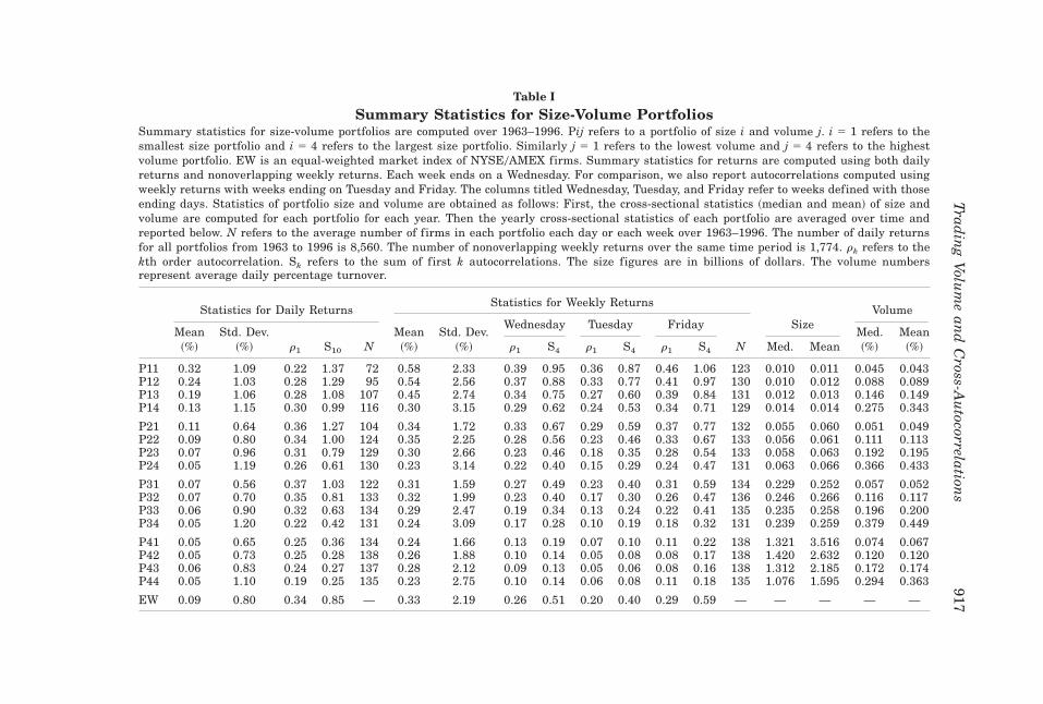
Table I

Summary Statistics for Size-Volume PortfoliosSummary statistics for size-volume portfolios are computed over 1963–1996. Pij refers to a portfolio of size i and volume j. i 5 1 refers to thesmallest size portfolio and i 5 4 refers to the largest size portfolio. Similarly j 5 1 refers to the lowest volume and j 5 4 refers to the highestvolume portfolio. EW is an equal-weighted market index of NYSE0AMEX firms. Summary statistics for returns are computed using both dailyreturns and nonoverlapping weekly returns. Each week ends on a Wednesday. For comparison, we also report autocorrelations computed usingweekly returns with weeks ending on Tuesday and Friday. The columns titled Wednesday, Tuesday, and Friday refer to weeks defined with thoseending days. Statistics of portfolio size and volume are obtained as follows: First, the cross-sectional statistics ~median and mean! of size andvolume are computed for each portfolio for each year. Then the yearly cross-sectional statistics of each portfolio are averaged over time andreported below. N refers to the average number of firms in each portfolio each day or each week over 1963–1996. The number of daily returnsfor all portfolios from 1963 to 1996 is 8,560. The number of nonoverlapping weekly returns over the same time period is 1,774. rk refers to thekth order autocorrelation. Sk refers to the sum of first k autocorrelations. The size figures are in billions of dollars. The volume numbersrepresent average daily percentage turnover.

Statistics for Weekly ReturnsStatistics for Daily Returns

Wednesday Tuesday Friday SizeVolume

Mean~%!

Std. Dev.~%! r1 S10 N

Mean~%!

Std. Dev.~%! r1 S4 r1 S4 r1 S4 N Med. Mean

Med.~%!

Mean~%!

P11 0.32 1.09 0.22 1.37 72 0.58 2.33 0.39 0.95 0.36 0.87 0.46 1.06 123 0.010 0.011 0.045 0.043P12 0.24 1.03 0.28 1.29 95 0.54 2.56 0.37 0.88 0.33 0.77 0.41 0.97 130 0.010 0.012 0.088 0.089P13 0.19 1.06 0.28 1.08 107 0.45 2.74 0.34 0.75 0.27 0.60 0.39 0.84 131 0.012 0.013 0.146 0.149P14 0.13 1.15 0.30 0.99 116 0.30 3.15 0.29 0.62 0.24 0.53 0.34 0.71 129 0.014 0.014 0.275 0.343

P21 0.11 0.64 0.36 1.27 104 0.34 1.72 0.33 0.67 0.29 0.59 0.37 0.77 132 0.055 0.060 0.051 0.049P22 0.09 0.80 0.34 1.00 124 0.35 2.25 0.28 0.56 0.23 0.46 0.33 0.67 133 0.056 0.061 0.111 0.113P23 0.07 0.96 0.31 0.79 129 0.30 2.66 0.23 0.46 0.18 0.35 0.28 0.54 133 0.058 0.063 0.192 0.195P24 0.05 1.19 0.26 0.61 130 0.23 3.14 0.22 0.40 0.15 0.29 0.24 0.47 131 0.063 0.066 0.366 0.433

P31 0.07 0.56 0.37 1.03 122 0.31 1.59 0.27 0.49 0.23 0.40 0.31 0.59 134 0.229 0.252 0.057 0.052P32 0.07 0.70 0.35 0.81 133 0.32 1.99 0.23 0.40 0.17 0.30 0.26 0.47 136 0.246 0.266 0.116 0.117P33 0.06 0.90 0.32 0.63 134 0.29 2.47 0.19 0.34 0.13 0.24 0.22 0.41 135 0.235 0.258 0.196 0.200P34 0.05 1.20 0.22 0.42 131 0.24 3.09 0.17 0.28 0.10 0.19 0.18 0.32 131 0.239 0.259 0.379 0.449

P41 0.05 0.65 0.25 0.36 134 0.24 1.66 0.13 0.19 0.07 0.10 0.11 0.22 138 1.321 3.516 0.074 0.067P42 0.05 0.73 0.25 0.28 138 0.26 1.88 0.10 0.14 0.05 0.08 0.08 0.17 138 1.420 2.632 0.120 0.120P43 0.06 0.83 0.24 0.27 137 0.28 2.12 0.09 0.13 0.05 0.06 0.08 0.16 138 1.312 2.185 0.172 0.174P44 0.05 1.10 0.19 0.25 135 0.23 2.75 0.10 0.14 0.06 0.08 0.11 0.18 135 1.076 1.595 0.294 0.363

EW 0.09 0.80 0.34 0.85 — 0.33 2.19 0.26 0.51 0.20 0.40 0.29 0.59 — — — — —

Trad

ing

Volum

ean

dC

ross-Au

tocorrelations

917

small size stocks are higher than usual because we drop daily returns ondays a stock does not trade. The first-order autocorrelation in daily portfolioreturns, r1, decreases with volume in each size quartile except in the small-est size quartile ~ r1 is 0.22 for portfolio P11 and 0.30 for portfolio P14!.7 Onthe other hand, the sum of the first 10 autocorrelations of the daily portfolioreturns is positive and declines monotonically with trading volume in eachsize portfolio.

Table I also reports autocorrelations for weekly portfolio returns with weeksending on Wednesday, Tuesday, and Friday. Consistent with the findings ofBoudoukh et al. ~1994!, we find that autocorrelations based on a Tuesdayclose are too low and those based on a Friday close are too high. The auto-correlations based on Wednesday close are not at either extreme and justifythe use of Wednesday close weekly returns. Therefore, all of our empiricalresults from Table II onward are based on Wednesday close weekly returns.The weekly autocorrelations, both at lag one and the sum of the first fourlags, decline monotonically with trading volume in each size portfolio.8

Not surprisingly, both daily and weekly autocorrelations also declinewith firm size. However, the autocorrelations remain fairly large even inthe largest size quartile, especially at the daily frequency. The first-orderautocorrelations for P41 at the daily and weekly frequencies are 0.25 and0.13 respectively. Predictably, the autocorrelations are lower using weeklyreturns.

If security prices adjust slowly to information, then price increases ~de-creases! will be followed by increases ~decreases!. This would give rise topositive autocorrelation in stock returns.9 The portfolio autocorrelation ev-idence in Table I ~except for four portfolios of size 1 involving daily re-turns! is, therefore, consistent with the hypothesis that returns of stockswith high trading volume adjust faster to common information. On theother hand, positive portfolio autocorrelations are also symptomatic of non-trading problems. However, as Boudoukh et al. ~1994! point out, even het-erogeneity in nontrading cannot explain all of the autocorrelations reportedin Table I. They estimate, for instance, that with extreme heterogeneity innontrading and betas, the first-order weekly autocorrelation implied bynontrading can be as high as 0.18. This is still less than half of the first-

7 One reason this happens is because of the way we compute portfolio returns. Note that wedrop firms that do not trade at day t or t 2 1 from the portfolio at day t. This throws awayvaluable information about delayed reaction to private information and reduces the autocorre-lations for the low turnover portfolio.

8 For P11, P12, and P13, the first-order daily autocorrelations are somewhat lower thanfirst-order weekly autocorrelations. This is the result of persistence in daily autocorrelations.The sum of the first 10 daily autocorrelations are, however, uniformly higher than the sum ofthe first four weekly autocorrelations.

9 Contrary to this hypothesis, most individual stocks exhibit a small negative autocorrelationin daily and weekly returns ~see Lo and MacKinlay ~1990!! but portfolio returns exhibit positiveautocorrelations.


order weekly autocorrelation of 0.39 estimated for P11 ~see Table I!. Forlarger size portfolios, where nontrading problems are minimal, the nontrading-implied autocorrelations are much smaller ~see Figure 2, p. 559 in Bou-doukh et al. ~1994!!. This suggests that nontrading issues cannot be thesole explanation for the autocorrelations in Table I and other evidence tobe presented in this paper.

Table I also reports the median and average size and the median andaverage trading volume for each portfolio. These are obtained by averagingthe annual cross-sectional statistics. As expected, the median and mean trad-ing volume increase within each size quartile. The median and mean size,however, increase with trading volume only in the first three size quartiles.In the largest size quartile ~size quartile 4!, the median and mean size de-crease with trading volume. This provides an opportunity to test whethertrading volume has an independent inf luence on the cross-autocorrelationspatterns. If trading volume has an independent effect then returns on highvolume stocks should continue to lead returns on low volume stocks even inthe largest size quartile. If, on the other hand, trading volume is simply aproxy of firm size then, in the largest size quartile, low volume portfolioreturns should lead high volume portfolio returns. The autocorrelation evi-dence in Table I suggests that trading volume has an independent effect onportfolio autocorrelations. Additional evidence in support of this is providedlater using tests based on cross-autocorrelations.

Finally, Table I reports the average number of firms in each portfolioeach day or week during 1963 to 1996. The daily averages are signifi-cantly lower for portfolios P11 and P12 ~small size, low trading volumeportfolios!, indicating that many small firms had to be dropped from dailyportfolios due to nontrading problems ~recall that when computing port-folio returns we drop returns of firms that did not trade today or yester-day!. However, as Table I shows, nontrading problems are minimal in thelarger size quartiles. Moreover, the weekly averages suggest that at theweekly frequency, nontrading problems are minimal even in the smallestsize quartile.

Although the autocorrelation evidence is consistent with the hypothesisthat the prices of high volume stocks adjust more rapidly to information,it is important to point out that autocorrelations are not likely to provideunambiguous inferences on the differences in speed of adjustment. Tosee this clearly, consider two stocks A and B. Suppose that the return onstock A responds to both today’s market information and yesterday’s marketinformation and the return on stock B responds only to yesterday’s marketinformation. Stock A, which adjusts faster to information, would exhibitpositive autocorrelation in daily returns. On the other hand, stock B,which adjusts more slowly to information, would exhibit zero autocorrela-tion. Cross-autocorrelations, on the other hand, do not suffer from this prob-lem. Therefore, in the rest of the paper, we focus our attention on differencesin cross-autocorrelations.


B. Empirical Tests

B.1. Vector Autoregressions

Following Brennan et al. ~1993!, we consider two types of time series tests:~1! vector autoregressions ~VARs!, and ~2! Dimson beta regressions. The VARtests are designed to address two questions: ~a! Do cross-autocorrelationshave information independent from own autocorrelations? ~b! Is the abilityof returns on high volume stocks to predict returns on low volume stocksbetter than the ability of returns on low volume stocks to predict returns onhigh volume stocks?

To understand the VAR tests, let us suppose that we want to test whetherreturns of portfolio B lead returns of portfolio A. The lead-lag effects be-tween the returns of these two portfolios can be tested using a bivariatevector autoregression:10

rA, t 5 a0 1 (k51

K

ak rA, t2k 1 (k51

K

bk rB, t2k 1 ut , ~1!

rB, t 5 c0 1 (k51

K

ck rA, t2k 1 (k51

K

dk rB, t2k 1 vt . ~2!

In regression ~1!, if lagged returns of portfolio B can predict current returnsof portfolio A, controlling for the predictive power of lagged returns of port-folio A, returns of portfolio B are said to granger cause returns of portfolio A.In our analysis, we use a modified version of the granger causality test byexamining whether the sum of the slope coefficients corresponding to returnB in equation ~1! is greater than zero.11 The granger causality test allowsus to determine if cross-autocorrelations are independent of portfolioautocorrelations.

Next, we are interested in testing formally whether the ability of laggedreturns of B to predict current returns of A is better than the ability oflagged returns of A to predict current returns of B. We test this hypothesisby examining if (k51

K bk in equation ~1! is greater than (k51K ck in equation

~2!. We refer to this test as the cross-equation test. This test is crucial toestablishing that returns of portfolio B lead returns of portfolio A and is aformal test of any asymmetry in cross-autocorrelations between high tradingvolume and low trading volume stocks.

10 Since the regressors are the same for both regressions, the VAR can be efficiently esti-mated by running ordinary least squares ~OLS! on each equation individually.

11 The usual version is to jointly test whether the slope coefficients corresponding to thelagged returns of the portfolio B are equal to zero. Our version tests not only for predictabilitybut also for the sign of predictability. Therefore, it is a more stringent test.


B.2. Dimson Beta Regressions

In the VAR tests, we control for size-related differences in speed of adjust-ment by forming four size portfolios and estimating the VAR within eachsize quartile. We control for other systematic effects in our tests of speed ofadjustment by running a market model regression suggested by Dimson ~1979!which includes leads and lags of market returns as additional independentvariables. The Dimson beta regressions allow us to analyze the pattern ofunder- or overreaction of portfolio returns to market returns. They also allowus to measure the speed of adjustment of each stock or portfolio relative toa single common benchmark, which is helpful in comparing the speed ofadjustment across individual stocks or portfolios. In contrast, the VAR testsmeasure speed of adjustment of two portfolios relative to one another.However, both VAR and Dimson beta regressions do capture similar lead-lageffects.

In order to understand the Dimson beta regressions, consider a zero netinvestment portfolio O that is long in portfolio B and short in portfolio A.Now consider a regression of the return on the zero net investment portfolioon leads and lags of the return on the market portfolio:

rO, t 5 aO 1 (k52K

K

bO, k rm, t2k 1 uO, t , ~3!

where bO, k 5 bB, k 2 bA, k. It is easy to show that portfolio B adjusts morerapidly to common information than portfolio A if and only if the contem-poraneous beta of portfolio B, bB,0, is greater than the contemporaneousbeta of portfolio A, bA,0, and the sum of the lagged betas of portfolio B,(k51

K bB, k , is less than the sum of the lagged betas of portfolio A, (k51K bA, k .

In terms of the regression in equation ~3!, this translates into examiningwhether bO,0 . 0 and (k51

K bO, k , 0. The basic intuition behind this resultis that if portfolio B responds more rapidly to marketwide informationthan portfolio A, its sensitivity to today’s common information ~market re-turn! should be greater than that of portfolio A. In the same vein, sinceportfolio A responds sluggishly to contemporaneous information, it shouldrespond more to past common information ~lagged market returns!. Theimportant thing to note here is that the speed of adjustment ~relative tothe market portfolio! is a function of both the contemporaneous beta andthe lagged betas.

B.3. Hypothesis Testing

Note that all the hypothesis tests discussed above are one-sided tests in-volving one-sided alternative hypotheses. In tests involving a single restric-tion, this can be easily handled using a traditional one-sided Z-test. However,in tests involving more than one restriction ~as in the case of joint testsinvolving a system of equations!, the regressions have to be estimated under


the constrained alternative hypothesis.12 This is what we do in this paper.The resulting Wald test statistic, however, is not distributed as the tradi-tional x2 with the appropriate number of degrees of freedom but as a mix-ture of chi-square distributions ~see Gourieroux, Holly, and Monfort ~1982!!.Specifically, a one-sided test with m restrictions has the following distribution:

Wm ; (j50

m

wj xj2, ~4!

where 0 , wj , 1. The complication is that wj is a complex, nonlinear func-tion of the data and depends on the particular alternative hypothesis. There-fore, there are no general closed-form solutions for the weight function.However, as pointed out by Gourieroux et al., a one-sided test that takes intoaccount the constrained alternative hypothesis ought to have better powercharacteristics than a two-sided test. This suggests that hypothesis teststhat use the distribution in equation ~4! should be able to reject the nullhypothesis more often than those that use the traditional chi-square distri-bution. This in turn suggests that if we are able to reject the null hypothesisagainst the one-sided alternative hypothesis using the traditional chi-squaredistribution, then we should most likely be able to reject the null hypothesisusing the mixture of chi-square distributions.13 This is the approach we adoptfor the purpose of hypothesis testing.

In the next section, we discuss three pieces of evidence: ~a! own autocor-relations and cross-autocorrelations, ~b! results from VAR regressions andgranger causality tests, and ~c! results from Dimson beta regressions.

II. Empirical Results

A. Cross-Autocorrelations and Own Autocorrelations

Table II presents cross-autocorrelations for size-volume portfolio returns.Panel A presents cross-autocorrelations for daily portfolio returns and PanelB presents cross-autocorrelations for weekly portfolio returns with weeksending on a Wednesday. The correlations are computed using only the ex-treme trading volume portfolios within each size quartile. The results showthat, in every size quartile, the correlation between lagged high volume port-folio returns, ri4, t21, and current low volume portfolio returns, ri1, t , is al-ways larger than the correlation between lagged low volume portfolio returns,ri1, t21, and current high volume portfolio returns, ri4, t . For instance, in thelargest size quartile, using daily returns ~see Panel A!, the correlation be-

12 We thank the referee for pointing this out.13 Gourieroux et al. ~1982! provide results on the power characteristics of the constrained

test only for the case of the single constraint. They also provide critical statistics only for thetwo-constraint case and that too for limited parameter values. Computing the critical statisticsor examining the power characteristics for tests involving more than two constraints is beyondthe scope of this paper.


tween lagged high volume portfolio returns, r44, t21, and the contemporane-ous low volume portfolio returns, r41, t , is 0.30 while the correlation betweenlagged low volume portfolio returns, r41, t21, and the contemporaneous highvolume portfolio returns, r44, t , is only 0.12. Similarly, using weekly returns~see Panel B!, the correlation between r44, t21 and r41, t is 0.15 and the cor-relation between r41, t21, and r44, t is only 0.06. The fact that we observethese lead-lag patterns in the largest size quartile using both daily and weeklyreturns suggests that nonsynchronous trading cannot be the only source ofthese lead–lag patterns.

Based on a simple AR~1! model of portfolio returns suggested by Bou-doukh et al. ~1994!, we examine whether cross-autocorrelations are simplyan inefficient way of describing the high autocorrelations of low volumeportfolios.14 In the context of the size-volume portfolios, the AR~1! model

14 Boudoukh et al. ~1994! specify an AR~1! model for the return-generating process for eachsize portfolio where the AR~1! parameter is positive and declines monotonically with size. Theshocks to the AR~1! process are assumed to be white noise but are contemporaneously corre-lated across size portfolios. It is important to point out that the AR~1! model, by assumption,rules out independent cross-autocorrelations between portfolio returns.

Table II

Size-Volume Portfolio Cross-Autocorrelationsrij, t refers to the time t return of a portfolio corresponding to the ith size quartile and the jthvolume quartile within the ith size quartile. The number of daily observations between 1963and 1996 is 8,560. The number of nonoverlapping weekly observations between 1963 and 1996is 1,774. Each week ends on a Wednesday. Panels A and B report cross-autocorrelations at thefirst lag.

r11, t r14, t r21, t r24, t r31, t r34, t r41, t r44, t

Panel A: Daily Returns

r11, t21 0.22 0.24 0.29 0.14 0.25 0.10 0.12 0.06r14, t21 0.35 0.30 0.39 0.21 0.35 0.14 0.17 0.09r21, t21 0.31 0.27 0.36 0.17 0.34 0.11 0.16 0.06r24, t21 0.34 0.36 0.44 0.26 0.41 0.19 0.23 0.13r31, t21 0.30 0.28 0.39 0.19 0.37 0.13 0.19 0.08r34, t21 0.33 0.36 0.45 0.29 0.44 0.22 0.26 0.16r41, t21 0.27 0.27 0.39 0.22 0.42 0.17 0.25 0.12r44, t21 0.31 0.35 0.45 0.30 0.46 0.25 0.30 0.19

Panel B: Weekly Returns

r11, t21 0.39 0.25 0.28 0.15 0.20 0.11 0.05 0.04r14, t21 0.43 0.29 0.32 0.19 0.24 0.12 0.08 0.05r21, t21 0.40 0.28 0.33 0.19 0.27 0.13 0.10 0.06r24, t21 0.40 0.32 0.35 0.22 0.28 0.15 0.12 0.08r31, t21 0.37 0.26 0.33 0.19 0.27 0.13 0.12 0.07r34, t21 0.38 0.32 0.36 0.24 0.31 0.17 0.14 0.10r41, t21 0.30 0.22 0.30 0.17 0.27 0.12 0.13 0.06r44, t21 0.34 0.29 0.34 0.23 0.30 0.16 0.15 0.10


would predict that the correlation between the lagged returns of the highvolume portfolio, ri4, t21, and the current returns of the low volume portfolio,ri1, t , should be less than or equal to the autocorrelation in the returns of thelow volume portfolio, ri1, t ; that is, corr~ri1, t , ri4, t21! # corr~ri1, t , ri1, t21!. Inother words, the model predicts that the low volume portfolio returns’ auto-correlations should be larger than their cross-autocorrelations with laggedhigh volume returns.

The results in Table II show that in every size quartile, for low volume port-folios Pi1, cross-autocorrelations with lagged high volume portfolio returnsexceed own autocorrelations; that is, corr~ri1, t , ri4, t21! . corr~ri1, t , ri1, t21!.For instance, in Panel B, in size quartile 1, corr~r11, t , r14, t21! is 0.43 andcorr~r11, t , r11, t21! is 0.39. The same pattern is seen in every size quartileregardless of whether we use daily or weekly returns. These results clearlyindicate that cross-autocorrelations contain independent information aboutdifferences in speed of adjustment. We establish this more formally in thenext section using vector autoregression tests.

Contrast the above result with cross-autocorrelations related only to sizedifferences as seen in Panel B of Table II. Consider portfolios P11 and P41,which are extreme size quartile portfolios. In examining the lead-lag pat-terns between the returns of these two portfolios, we find that the autocor-relation in the returns of P11, corr~r11, t , r11, t21! 5 0.39, exceeds the correlationbetween lagged returns of P41 and current returns of P11, corr~r41, t21, r11, t ! 50.30. This is what Boudoukh et al. ~1994! report in their paper and why theyconclude that cross-autocorrelations are not as important as own autocorre-lations in size-sorted portfolios.

B. Vector Autoregressions

We estimate the VAR using daily or weekly returns of the two extremevolume portfolios in each size quartile: ~P11, P14!, ~P21, P24!, ~P31, P34!,and ~P41, P44!. With daily returns, the VAR is estimated using five lags,K 5 5.15 With weekly returns, the VAR is estimated with one lag ~K 5 1!because additional lags only add noise. All regressions are estimated withthe White heteroskedasticity correction for standard errors. The White cor-rection and the use of lagged dependent variables as regressors result in theuse of asymptotic statistics for making statistical inferences. Table III sum-marizes the results from the four VAR regressions. Low and High representthe sum of the slope coefficients of the lagged returns on the low volumeportfolio and the lagged returns on the high volume portfolio, respectively.L1 and H1 represent the slope coefficients of the one-lag returns of the lowvolume portfolio and the high volume portfolio ~a1 and b1 or c1 and d1!,respectively. Panel A presents VAR results using daily returns and Panel Bpresents VAR results using weekly returns.

15 The results for 10 lags are similar.


Table III

Vector Autoregressions for the Size-Volume PortfoliosThe following VAR is estimated using daily or weekly data from 1963 to 1996:

rA, t 5 a0 1 (k51

K

ak rA, t2k 1 (k51

K

bk rB, t2k 1 ut ,

rB, t 5 c0 1 (k51

K

ck rA, t2k 1 (k51

K

dk rB, t2k 1 vt .

The LHS variable is the return on the lowest ~rA, t ! or the highest ~rB, t ! volume portfolio withineach size quartile. The portfolios Pij are defined in Table 1. Low refers to (k51

K ak or (k51K ck

and High refers (k51K bk or (k51

K dk as per the dependent variable. Similarly, L1 denotes a1 or c1

and H1 denotes b1 or d1. OR2 is the adjusted coefficient of determination. NOBS refers to thenumber of daily or weekly returns used in the regressions. Z~A! is the Z-statistic correspondingto the cross-equation null hypothesis (k51

K bk 5 (k51K ck in each bivariate VAR. The alternative

hypothesis is (k51K bk . (k51

K ck . K 5 5 ~K 5 1! for regressions involving daily ~weekly! returns.The significance levels for Z~A! are based on upper-tail tests. WA, m

U ~WA, mC ! is the Wald test

statistic corresponding to the joint-test of null hypothesis across all equations against an un-constrained ~inequality constrained) alternative hypothesis. m is the number of constraints~degrees of freedom! of the test. All statistics are computed based on White heteroskedasticitycorrected standard errors.

Panel A: Daily Returns ~NOBS 5 8,555!

LHS L1 Low H1 High OR2 Z~A!

P11 20.0308*** 0.1524* 0.3053* 0.4511* 0.16 5.05*P14 0.0767* 0.1565* 0.2466* 0.3289* 0.11

P21 20.0343 0.1942* 0.2429* 0.2507* 0.22 3.05*P24 20.1798** 20.0912 0.3310* 0.4067* 0.08

P31 0.0240 0.1633*** 0.1943* 0.2129* 0.21 3.18*P34 20.2645* 20.3154** 0.3157* 0.4541* 0.06

P41 0.0161 0.0111 0.1706* 0.1993* 0.09 3.97*P44 20.2160* 20.3758* 0.3032* 0.4371* 0.05

Joint Test: WA,4U 5 WA,4

C 5 75.15*

Panel B: Weekly Returns ~NOBS 5 1,773!

LHS L1 H1 OR2 Z~A!

P11 0.1195** 0.2423* 0.19 1.92**P14 0.0512 0.2610* 0.08

P21 0.0867 0.1506* 0.12 1.18P24 20.0563 0.2477* 0.05

P31 0.0477 0.1374* 0.09 1.37***P34 20.0889 0.2045* 0.03

P41 0.0088 0.0836* 0.02 1.66**P44 20.1413 0.1704* 0.01

Joint Test: WA,4U 5 WA,4

C 5 24.21*

*, **, and *** denote significance at the 1, 5, and 10 percent levels, respectively.


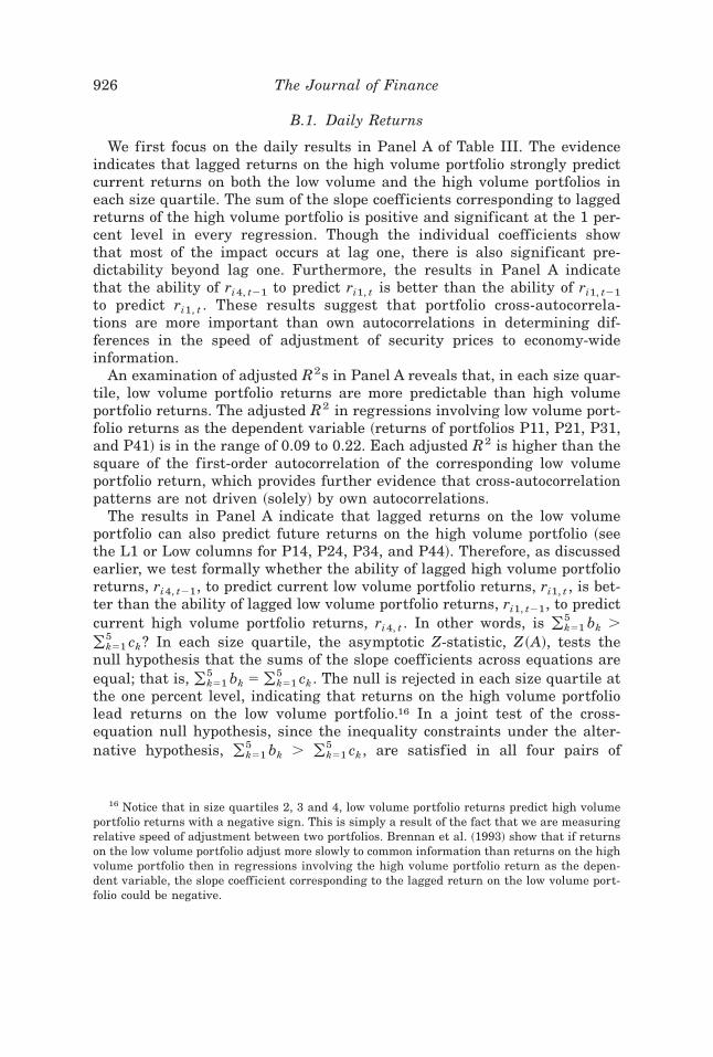
B.1. Daily Returns

We first focus on the daily results in Panel A of Table III. The evidenceindicates that lagged returns on the high volume portfolio strongly predictcurrent returns on both the low volume and the high volume portfolios ineach size quartile. The sum of the slope coefficients corresponding to laggedreturns of the high volume portfolio is positive and significant at the 1 per-cent level in every regression. Though the individual coefficients showthat most of the impact occurs at lag one, there is also significant pre-dictability beyond lag one. Furthermore, the results in Panel A indicatethat the ability of ri4, t21 to predict ri1, t is better than the ability of ri1, t21to predict ri1, t . These results suggest that portfolio cross-autocorrela-tions are more important than own autocorrelations in determining dif-ferences in the speed of adjustment of security prices to economy-wideinformation.

An examination of adjusted R2s in Panel A reveals that, in each size quar-tile, low volume portfolio returns are more predictable than high volumeportfolio returns. The adjusted R2 in regressions involving low volume port-folio returns as the dependent variable ~returns of portfolios P11, P21, P31,and P41! is in the range of 0.09 to 0.22. Each adjusted R2 is higher than thesquare of the first-order autocorrelation of the corresponding low volumeportfolio return, which provides further evidence that cross-autocorrelationpatterns are not driven ~solely! by own autocorrelations.

The results in Panel A indicate that lagged returns on the low volumeportfolio can also predict future returns on the high volume portfolio ~seethe L1 or Low columns for P14, P24, P34, and P44!. Therefore, as discussedearlier, we test formally whether the ability of lagged high volume portfolioreturns, ri4, t21, to predict current low volume portfolio returns, ri1, t , is bet-ter than the ability of lagged low volume portfolio returns, ri1, t21, to predictcurrent high volume portfolio returns, ri4, t . In other words, is (k51

5 bk .

(k515 ck? In each size quartile, the asymptotic Z-statistic, Z~A!, tests the

null hypothesis that the sums of the slope coefficients across equations areequal; that is, (k51

5 bk 5 (k515 ck . The null is rejected in each size quartile at

the one percent level, indicating that returns on the high volume portfoliolead returns on the low volume portfolio.16 In a joint test of the cross-equation null hypothesis, since the inequality constraints under the alter-native hypothesis, (k51

5 bk . (k515 ck , are satisfied in all four pairs of

16 Notice that in size quartiles 2, 3 and 4, low volume portfolio returns predict high volumeportfolio returns with a negative sign. This is simply a result of the fact that we are measuringrelative speed of adjustment between two portfolios. Brennan et al. ~1993! show that if returnson the low volume portfolio adjust more slowly to common information than returns on the highvolume portfolio then in regressions involving the high volume portfolio return as the depen-dent variable, the slope coefficient corresponding to the lagged return on the low volume port-folio could be negative.


regressions, the unconstrained Wald test statistic and the constrained Waldtest statistic are the same; that is, WA,U 5 WA,C 5 75.15. The Wald teststatistics reject the joint null hypothesis at the one percent level. Overall,the results provide strong evidence that returns on high volume portfolioslead returns on low volume portfolios.

A brief discussion of the economic significance of the results in Panel A isin order here. Focusing on the P41 regression in the largest size quartile~because these are the most liquid stocks!, on average, a one percent in-crease in today’s return of high volume stocks, P44, all else equal, leads to a0.1706 percent increase in tomorrow’s return of low volume stocks, P41. Thedaily standard deviation of the high volume portfolio return is 1.10 percent.Therefore, a one percent increase is within one standard deviation. The0.1706 percent increase in the returns of the low volume portfolio is approx-imately three times above its daily mean of 0.05 percent. This suggests thatthese lead-lag cross-autocorrelations effects could be economically signifi-cant. Similarly a one percent increase in the low volume portfolio return,P41, leads to a 0.2160 percent decrease ~conditionally! in the high volumeportfolio return, P44, which is again economically significant given its dailymean of 0.05 percent.

B.2. Weekly Returns

Foerster and Keim ~1998! report that since 1963 less than one percent ofthe stocks in the three largest size deciles in the NYSE and AMEX did nottrade on a given day. The results in Panel A show that the lead-lag cross-autocorrelations between high volume and low volume portfolio returns areas strong in the largest size quartile as they are in the smallest size quar-tile. This makes it unlikely that these results could be due to nonsynchro-nous trading.

In order to allay any remaining concerns about nonsynchronous trading,however, we repeat the VAR tests using weekly portfolio returns. The re-sults involving weekly portfolio returns are presented in Panel B of Table III.The VAR is estimated with one lag because additional lags only add noise.The results in Panel B show that high volume portfolio returns lead lowvolume portfolio returns even at the weekly frequency. In every size quar-tile, lagged returns on the high volume portfolio exhibit statistically andeconomically significant predictive power for future returns on the low vol-ume portfolio. In contrast, lagged returns on the low volume portfolio ex-hibit little or no ability to predict future returns on the high volume portfolioand only weak ability to predict returns on the low volume portfolio. Onceagain the joint test statistic for the cross-equation null hypothesis A is sig-nificant at the 1 percent level. Overall, the weekly results closely parallelthe daily results and make it unlikely that nonsynchronous trading could bethe primary explanation for the lead-lag cross-autocorrelations reported inthis paper.


B.3. Additional Robustness Checks

As a final check to see if nontrading inf luences our results, we estimatethe VAR at both the daily and the weekly frequencies using only post-1980data. The results ~not reported in the paper! are similar to those in Table IIIand strongly support the hypothesis that returns on the high volume port-folio lead returns on the low volume portfolio.

One potential criticism of these results, given the positive correlation be-tween firm size and volume ~a correlation of 0.15 in our sample!, is thattrading volume simply proxies for firm size. We address this issue in twoways. First, recall that volume and size are negatively correlated in sizequartile 4 ~see Table I!. Therefore, if the cross-autocorrelation results withrespect to volume are being driven by firm size, we should see returns onportfolio P41 lead returns on portfolio P44. Yet the cross-autocorrelations inTable II indicate that the correlation is higher between lagged returns ofP44 and current returns of P41 than between lagged returns of P41 andcurrent returns of P44. Moreover, the VAR results in Table III confirm thatreturns on P44 lead returns on P41.

Next, we choose high and low volume portfolios from adjacent size quar-tiles to ensure that portfolio size and volume are negatively correlated. Con-sider the following three pairs of portfolios: ~P21, P14!, ~P31, P24!, and ~P41,P34!. In each of these pairs, firm size and volume are negatively correlated.For instance, the average size of P21 is about four times that of P14 ~seeTable I! but the average volume of P21 is only about one-fifth that of P14.The negative correlation between size and volume allows us to see whetherthe volume effect is independent of the size effect in determining lead-lagcross-autocorrelations. Now let us return to the cross-autocorrelation evi-dence in Table II. In both Panel A and Panel B, the correlation betweenlagged returns of the high volume portfolio ~P14, P24, or P34! and currentreturns of the low volume portfolio ~P21, P31, or P41! is higher than thecorrelation between lagged returns of the low volume portfolio ~P21, P31, orP41! and current returns of the high volume portfolio ~P14, P24, or P34!.This suggests that the volume effect is independent of the size effect. Wealso perform VAR tests involving the three pairs of low and high volumeportfolios from adjacent size quartiles. The regression results ~not reported!are similar to those in Table III.

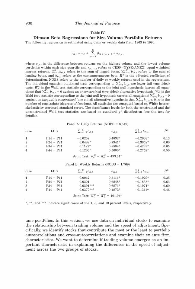
C. Dimson Beta Regressions

As discussed in Section B.2, we use zero investment portfolios in the Dim-son beta regressions. The zero investment portfolios are constructed by sub-tracting low volume portfolio returns from high volume portfolio returns.Since we expect high volume portfolio returns to adjust faster to commonfactor information than do low volume portfolio returns, the contemporane-ous betas from these regressions, bO,0, should be positive and the sum oflagged betas, (k51

K bO, k should be negative. The intuition behind these re-strictions is as follows. If the return on the high volume portfolio responds


more rapidly to common information than the return on the low volumeportfolio then its sensitivity to today’s common information ~market return!should be greater than that of the low volume portfolio. Therefore, thecontemporaneous beta of the zero investment portfolio should be positive.Additionally, since the low volume portfolio responds sluggishly to contem-poraneous factor information ~current market returns!, it should respondmore to past common factor information ~lagged market returns!. Therefore,the lagged betas of the zero investment portfolio should be negative.

We estimate the Dimson beta regressions in equation ~3! using the NYSE0AMEX equal-weighted portfolio return as a proxy for the common factor.17

All standard errors are corrected for generalized heteroskedasticity usingthe White correction. Table IV presents results from Dimson beta regres-sions. Panel A reports results using daily returns and Panel B reports re-sults using weekly returns. We use five leads and lags of market returns indaily Dimson beta regressions and two leads and lags of market returns inweekly Dimson beta regressions.18

First, we focus on the daily results in Panel A. The contemporaneous betasof the zero investment portfolio, bO,0, are positive and significant at the onepercent level in each size quartile. Also, the sum of the lagged betas is sig-nificantly negative in each size quartile. These results indicate that, in eachsize quartile, the returns on the low volume portfolio adjust more slowly tomarketwide information than the returns on the high volume portfolio. Notsurprisingly, both the constrained and the unconstrained Wald test statisticsstrongly reject the joint null hypothesis that the sum of the lagged betas iszero in each size quartile, at the one percent level. The sum of leading betasindicates that current returns on the zero investment portfolios in size quar-tiles 2, 3, and 4 are able to predict future returns of the equal-weightedmarket index. This suggests that returns on high volume portfolios in thelarger size quartiles lead returns on the equal-weighted market index. Theweekly results in Panel B are similar to the daily results and reveal signif-icant differences in speed of adjustment related to trading volume. Overall,the results indicate that the lead-lag cross-autocorrelations observed be-tween high volume and low volume stocks are driven by differences in thespeed of adjustment to common factor information.

III. Speed of Adjustment of Individual Stocks

Up to this point our empirical tests use portfolio returns to examine therelationship between cross-sectional differences in trading volume and speedof adjustment to common information. We find that returns of high volumeportfolios adjust faster to marketwide information than do those of low vol-

17 We also perform all regressions reported in Table IV using the CRSP value-weightedmarket index and the results are similar.

18 For daily returns, the results with 10 leads and lags are similar. For weekly returns, theuse of additional lags only adds more noise to statistical inference.


ume portfolios. In this section, we use data on individual stocks to examinethe relationship between trading volume and the speed of adjustment. Spe-cifically, we identify stocks that contribute the most or the least to portfolioautocorrelations and cross-autocorrelations and examine their ex ante firmcharacteristics. We want to determine if trading volume emerges as an im-portant characteristic in explaining the differences in the speed of adjust-ment across the two groups of stocks.

Table IV

Dimson Beta Regressions for Size-Volume Portfolio ReturnsThe following regression is estimated using daily or weekly data from 1963 to 1996:

rO, t 5 aO 1 (k52K

K

bO, k rm, t2k 1 uO, t ,

where rO, t is the difference between returns on the highest volume and the lowest volumeportfolios within each size quartile and rm, t2k refers to CRSP ~NYSE0AMEX! equal-weightedmarket returns. (k51

K bO, k refers to the sum of lagged betas, (k5212K bO, k refers to the sum of

leading betas, and bO,0 refers to the contemporaneous beta. OR2 is the adjusted coefficient ofdetermination. NOBS refers to the number of daily or weekly returns used in the regressions.The individual equation statistical tests corresponding to (k51

K bO, k are lower tail ~one-sided!tests. Wm

U is the Wald test statistic corresponding to the joint null hypothesis ~across all equa-tions! that (k51

K bO, k 5 0 against an unconstrained ~two-sided! alternative hypothesis. WmC is the

Wald test statistic corresponding to the joint null hypothesis ~across all equations! (k51K bO, k 5 0

against an inequality constrained ~one-sided! alternative hypothesis that (k51K bO, k # 0. m is the

number of constraints ~degrees of freedom!. All statistics are computed based on White hetero-skedasticity corrected standard errors. The significance levels for both the constrained and theunconstrained Wald test statistics are based on standard x2 distribution ~see the text fordetails!.

Panel A: Daily Returns ~NOBS 5 8,549!

Size LHS (k52125 bO, k bO,0 (k51

5 bO, k OR2

1 P14 2 P11 20.0252 0.4832* 20.2688* 0.132 P24 2 P21 0.0489* 0.7941* 20.3652* 0.603 P34 2 P31 0.1122* 0.8584* 20.4239* 0.654 P44 2 P41 0.1286* 0.5600* 20.2752* 0.50

Joint Test: W4U 5 W4

C 5 493.31*

Panel B: Weekly Returns ~NOBS 5 1,769!

Size LHS (k52122 bO, k bO,0 (k51

2 bO, k OR2

1 P14 2 P11 0.0067 0.5114* 20.1929* 0.352 P24 2 P21 0.0301 0.6848* 20.1858* 0.633 P34 2 P31 0.0391*** 0.6871* 20.1971* 0.604 P44 2 P41 0.0372*** 0.4872* 20.1311* 0.46

Joint Test: W4U 5 W4

C 5 101.94*

*, **, and *** indicate significance at the 1, 5, and 10 percent levels, respectively.


The sample used in this section contains all stocks available at the inter-section of CRSP NYSE0AMEX files and annual IBES files from 1976 to1996. We use the IBES files in order to obtain the number of analysts mak-ing annual earnings forecasts. The sample contains a total of 24,704 firmyears, or an average of approximately 1,200 firms per year.

To identify stocks that contribute the most ~or least! to portfolio autocor-relations and cross-autocorrelations we use a measure of speed of adjust-ment based on contemporaneous and lagged betas from Dimson betaregressions. Each year, from 1977 to 1996, the following Dimson beta re-gression is estimated for each stock in the sample:

ri, t 5 ai 1 (k525

5

bi, k rm, t2k 1 ui, t , ~5!

where ri, t is the daily return on the stock, rm, t is the daily return on themarket index, and bi, k is the beta with respect to the market return at lagk. We use the NYSE0AMEX equal-weighted market index as a proxy of themarket portfolio. Tests involving NYSE, AMEX, and Nasdaq value-weightedmarket indexes provide similar results.

Recall our discussion in Section B.2 that the speed of adjustment ~relativeto the market portfolio! is a function of both contemporaneous and laggedbetas. For simplicity consider a Dimson beta regression with just one lagand one lead. In comparing the speed of adjustment of two stocks A and B,returns of stock B are said to adjust more rapidly to common informationthan do returns of stock A if and only if stock B’s contemporaneous beta,bB,0, is greater than stock A’s contemporaneous beta, bA,0, and stock B’slagged beta, bB,1, is less than stock A’s lagged bA,1. We can state this resultin a more parsimonious way as follows. Returns of stock B adjust morerapidly to common information than do returns on stock A if and only ifbB,10bB,0, is less than bA,10bA,0.

For a Dimson beta regression with five leads and five lags, the speed ofadjustment ratio is defined to be (k51

5 bj, i, k 0bj, i,0. We use a logit transfor-mation of this ratio as our measure of speed of adjustment:

DELAYi 51

1 1 e2x , ~6!

where

x 5(k51

5

bi, k

bi,0.

Our measure is a modification of a measure proposed by McQueen et al.~1996!. If x is the ratio of lagged beta to contemporaneous beta then themeasure proposed by McQueen et al. is equal to the logit transformation ofx0~1 1 x!. Though this measure is monotonic in x for x . 1, it is nonmono-


tonic in x for x , 1. x is often less than one when measuring the speed ofadjustment of large stocks relative to the equal-weighted market index. Thisis because large stocks adjust faster to common information than the equal-weighted market index. As a result, for a large stock the contemporaneousbeta tends to be greater than one and the lagged beta tends to be negativeand less than one. This creates a problem in comparing a positive value of xto a negative value of x or in comparing two negative values of x. For x . 0our DELAY measure provides values greater than 0.5, and for x , 0 ourmeasure provides values less than 0.5.

The logit transformation has several appealing properties. First, it is mono-tonic in x. Secondly, the transformation moderates the inf luence of outliersand yields values between zero and one. Values closer to zero imply a fasterspeed of adjustment and values closer to one imply a slower speed of adjust-ment. Therefore, stocks with high ~low! DELAY are likely to contribute most~least! to portfolio autocorrelations and cross-autocorrelations. We use thismeasure to examine the cross-sectional relation between trading volume andthe speed of adjustment of individual stocks.

Next, for each firm in the sample, we match the DELAY measure com-puted in year t with firm characteristics as of year t 2 1. The firm charac-teristics are Volume, defined as the average number of shares traded per dayduring year t 2 1; Turnover, defined as the average daily turnover in per-centage during year t 2 1; Size, which is the market capitalization in mil-lions of dollars as of the December of year t 2 1; Price, which is the stockprice as of December of year t 2 1; Stdret, defined as the standard deviationof daily returns in percentage during year t 2 1; Nana, which is the numberof security analysts making annual forecasts as of the September of yeart 2 1; and Spread, defined as the average of the beginning and end-of-yearrelative spread in percent.19 The data on relative spread are the same asthose used in Eleswarapu and Reinganum ~1993!; they are available only forthe 1980 to 1989 time period and cover only NYSE stocks.

Finally, each year, we form four size quartiles and then divide each sizequartile into four quartiles based on DELAY. We focus our attention on theextreme DELAY quartiles, High and Low, within each size quartile. Highrepresents 25 percent of stocks within each size quartile that are likely tocontribute the most to delayed reaction to common factor information, Lowrepresents 25 percent of stocks that are likely to contribute the least todelayed reaction to common factor information. For each portfolio, each year,we compute the median ex ante firm characteristic and then average theannual medians over time.

The results are reported in Table V. In general, in each size quartile,both raw trading volume ~Volume! and relative trading volume ~Turnover!differ significantly across the two DELAY portfolios, High and Low. Onaverage, the raw trading volume for the high DELAY portfolio, High, is 25 per-

19 Relative spread is defined as the ratio of the dollar bid-ask spread to the average of thebid and ask prices.


cent to 45 percent lower than the raw trading volume for the low DELAYportfolio, Low. Similarly, the turnover for the high DELAY portfolio is,on average, 20 percent to 35 percent lower than the turnover for the lowDELAY portfolio. An exception is size quartile 4, in which there is not muchdifference in turnover across the two DELAY portfolios. This probably resultsfrom the fact that in size quartile 4, turnover and size tend to be negativelycorrelated ~see Table 1!. Additionally, Dimson beta estimators are likely tobe very noisy for individual stocks. This can be seen from the results inTable IV where, using portfolio returns, we find significant differences inthe speed of adjustment between high turnover and low turnover portfolios.

Table V

Speed of Adjustment and Ex Ante Firm CharacteristicsThis table provides time-series averages of the annual portfolio medians of the speed of adjust-ment measure DELAY and other ex ante firm characteristics. The sample period is 1976–1996and the sample size is 24,704 firm-years. The speed of adjustment measure, DELAY, defined inequation ~6!, is computed by running the Dimson beta regression in equation ~5! for each stockeach year. DELAY is constructed to be between zero and one where higher values representthose stocks contributing the most to portfolio cross-autocorrelations ~slower speed of adjust-ment! and lower values represent those stocks contributing the least to portfolio cross-autocorrelations ~faster speed of adjustment!. The NYSE0AMEX equal-weighted market indexis used as the proxy of the market index. At the beginning of each year all stocks available atthe intersection of NYSE0AMEX and annual IBES files are divided first into four quartileportfolios based on firm size as of the December of the previous year. Size 1 represents thesmallest size quartile and size 4 represents the largest size quartile. Each size quartile isfurther divided into four quartile portfolios based on DELAY computed from daily returns forthat year. In each size quartile we focus our attention on the extreme DELAY quartiles. Highrepresents 25 percent of stocks with the highest DELAY measure and Low represents 25 per-cent of stocks with the smallest DELAY measure within each size quartile. Each DELAY port-folio contains, on average, 77 stocks. The ex ante portfolio characteristics for these portfoliosare reported below. Size is the market capitalization as of the December of the previous year inmillions of dollars, Volume is the average number of shares traded per day over the previousyear, Turnover is the average daily turnover in percentage over the previous year, Nana is thenumber of security analysts making annual earnings forecasts as of the September of the pre-vious year, Price is the stock price as of the December of the previous year, Stdret is the stan-dard deviation of daily returns over the previous year in percentage, and Spread is the averagerelative spread for the stock in the previous year also in percentage.

SizeDelayedReaction DELAY Volume Turnover Size Price Stdret Nana Spread

1 ~Small! Low 0.35 11777 0.193 64.22 9.64 2.83 1.93 2.36High 0.70 6422 0.132 54.11 12.02 2.39 1.85 2.08

2 Low 0.34 27342 0.217 243.43 18.59 2.30 5.18 1.43High 0.65 15663 0.146 223.76 22.16 1.83 4.38 1.34

3 Low 0.33 61394 0.206 742.95 25.58 1.85 11.15 1.04High 0.58 46238 0.169 664.29 29.31 1.71 8.93 0.98

4 ~Large! Low 0.30 209481 0.187 3662.73 39.11 1.56 21.48 0.63High 0.50 128966 0.194 2214.57 39.30 1.62 16.95 0.71


To allay any remaining concerns that our results are driven by the smallilliquid stocks, we focus our attention on the results for the smallest sizequartile–highest DELAY portfolio. The time-series average of the mediandaily trading volume for the smallest size quartile–highest DELAY portfoliois 6,422 shares. The time-series average of the 25th percentile ~on averagethere are fewer than 20 stocks below this cutoff! daily trading volume of theabove portfolio is 3,244 shares. The time-series average of the fifth percen-tile ~fewer than four of the 77 stocks are below this cutoff! daily tradingvolume is 1,103 shares. For comparison, the fifth percentile daily tradingvolume for size quartiles 2, 3, and 4 ~the larger size portfolios! are 3,764shares, 8,705 shares, and 30,593 shares respectively. All these show that ourresults are not driven by extremely illiquid stocks.

Stocks with high DELAY also tend to be smaller, have fewer analysts, arehigher priced, and have lower volatility. Differences in relative spread acrosshigh and low DELAY stocks do not seem economically significant. In sum,the univariate statistics based on the speed of adjustment of individual stocksconfirm our earlier findings and strongly support the hypothesis that trad-ing volume is a significant determinant of how slowly or rapidly stock pricesadjust to new information.

IV. Conclusion

In this paper, we find that trading volume is a significant determinantof lead-lag cross-autocorrelations in stock returns. Specifically, returns ofportfolios containing high trading volume lead returns of portfolios com-prised of low trading volume stocks. Additional tests establish that thesource of these lead-lag cross-autocorrelations is the tendency of low vol-ume stock prices to react sluggishly to new information. While nontradingmay be a part of the story, the magnitude of the autocorrelations andcross-autocorrelations indicate that nontrading cannot be the sole explana-tion of our results.

At first glance these results may suggest some market inefficiency; how-ever, it is not clear that investors could profitably trade on these patternsbecause transaction costs are likely to overwhelm any potential profits. Thismight explain why these patterns do not get arbitraged away. Nevertheless,the results are interesting since they indicate a market in which tradingvolume plays a major role in the speed with which prices adjust to informa-tion, yielding insights into how stock prices become more informationallyefficient.

REFERENCES

Badrinath, Swaminathan G., Jayant R. Kale, and Thomas H. Noe, 1995, Of shepherds, sheepand the cross-autocorrelations in equity returns, Review of Financial Studies 8, 401–430.

Bessembinder, Hendrik, and Michael G. Hertzel, 1993, Return autocorrelations around non-trading days, Review of Financial Studies 6, 155–190.


Boudoukh, Jacob, Matthew P. Richardson, and Robert F. Whitelaw, 1994, A tale of three schools:Insights on autocorrelations of short-horizon stock returns, Review of Financial Studies 7,539–573.

Brennan, Michael J., Tarun Chordia, and Avanidhar Subrahmanyam, 1998, Alternative factorspecifications, security characteristics, and the cross-section of expected stock returns, Jour-nal of Financial Economics 49, 345–374.

Brennan, Michael J., Narasimhan Jegadeesh, and Bhaskaran Swaminathan, 1993, Investmentanalysis and the adjustment of stock prices to common information, Review of FinancialStudies 6, 799–824.

Campbell, John Y., Sanford J. Grossman, and Jiang Wang, 1993, Trading volume and serialcorrelation in stock returns, Quarterly Journal of Economics 107, 907–939.

Connolly, Robert A., and Chris T. Stivers, 1997, Time-varying lead-lag of equity returns in aworld of incomplete information, Working paper, University of North Carolina at ChapelHill.

Conrad, Jennifer, and Gautam Kaul, 1988, Time varying expected returns, Journal of Business61, 409–425.

Datar, Vinay, Narayan Naik, and Robert Radcliffe, 1998, Liquidity and asset returns: An alter-native test, Journal of Financial Markets 1, 203–220.

Dimson, Elroy, 1979, Risk measurement when shares are subject to infrequent trading, Journalof Financial Economics 7, 197–226.

Eleswarapu, Venkat R., and Marc R. Reinganum, 1993, The seasonal behaviour of the liquiditypremium in asset pricing, Journal of Financial Economics 34, 373–386.

Foerster, Stephen R., and Donald B. Keim, forthcoming, Direct evidence of non-trading of NYSEand AMEX stocks; in W. Ziemba and D. B. Keim, eds: Security Market Imperfections inWorldwide Equity Markets ~Cambridge University Press, New York!.

Gallant, Ronald A., Peter E. Rossi, and George Tauchen, 1992, Stock prices and volume, Reviewof Financial Studies 5, 199–242.

Gourieroux, Christian B., Alberto Holly, and Alain Monfort, 1982, Likelihood ratio test, Waldtest and Kuhn-Tucker test in linear models with inequality constraints on the regressionparameters, Econometrica 50, 63–80.

Hameed, Allaudeen, 1997, Time varying factors and cross-autocorrelations in short-horizon stockreturns, Journal of Financial Research 20, 435–458.

Jain, Prem C., and Gun-Ho Joh, 1988, The dependence between hourly prices and tradingvolume, Journal of Financial and Quantitative Analysis 23, 269–283.

Karpoff, Jonathan, 1987, The relation between price changes and trading volume: A survey,Journal of Financial and Quantitative Analysis 22, 109–126.

Keim, Donald B., and Robert F. Stambaugh, 1984, A further investigation of the weekend effectin stock returns, Journal of Finance 39, 819–834.

Lo, Andrew, and Craig MacKinlay, 1990, When are contrarian profits due to stock marketoverreaction?, Review of Financial Studies 3, 175–205.

McQueen, Grant, Michael Pinegar, and Steven Thorley, 1996, Delayed reaction to good newsand cross-autocorrelation of portfolio returns, Journal of Finance 51, 889–920.

Mech, Timothy S., 1993, Portfolio return autocorrelation, Journal of Financial Economics 34,307–344.


trading volume and cross-autocorrelations in stock …mkearns/finread/chordia_lead_lag.pdf ·...

Documents