trading in equity markets - biweb.bi.no/forskning/papers.nsf/0/b9f407d7eca4534dc... · trading in...
TRANSCRIPT

Trading in Equity MarketsA study of Individual, Institutional and Corporate
Trading Decisions
by
Johannes A. Skjeltorp
A dissertation submitted to BI Norwegian School of Management
for the Degree of Dr.Oecon
Series of Dissertations 8/2004
BI Norwegian School of Management
Department of Financial Economics
Johannes A. Skjeltorp:Trading in Equity Markets: A study of Individual, Institutional and Corporate TradingDecisions
c© Johannes A. Skjeltorp2004
Series of Dissertations 8/2004
ISBN: 82 7042 648 2ISSN: 1502-2099
BI Norwegian School of ManagementP.O.B. 580N-1302 SandvikaPhone: +47 67 55 70 00
Printing: Nordberg Hurtigtrykk
To be ordered from:
NorliPhone: +47 67 55 74 51Fax: +47 67 55 74 50Mail: [email protected]

To Kristin,and my parents Inger-Anne and Arne

iv

Acknowledgments
This thesis was written while I was at the Research Department of Norges Bank andduring my stay at the Leonard N. Stern School of Business at New York Universityfrom September 2001 to June 2002. I am very grateful to Norges Bank for its supportof my studies, my research as well as giving me the opportunity to spend a year doingresearch abroad.
The process of writing the dissertation has been much more frustrating and exhaust-ing than I ever imagined. However, I have been privileged to work on topics that I findexciting which has made the process extremely interesting and enjoyable. One veryimportant ingredient to the overall experience has been the many fascinating and kindpeople I have met, worked with and learnt to know during the years. They have en-couraged me, engaged in fruitful discussions and provided very useful suggestions thathas greatly contributed to my research.
The thesis is dedicated to my wife, Kristin, and my parents Inger-Anne and Arne.Kristin has been incredibly supportive, understanding and patient through the entireprocess. She also went with me to New York during my visit at the New York Uni-versity, which was a period I believe we will never forget. My parents have also beenvery encouraging and supportive throughout the process, and they deserve my warmestgratitude. In addition, I would like to express my thanks to all my fabulous friends forsticking out with me all these years, and continuously reminding me that there are infact more important things in life than my doctoral work.
I am very grateful to my supervisor Bernt Arne Ødegaard, who is also the co-authoron the last essay in the thesis. His penetrating comments have been very crucial andextremely valuable for the progress of my dissertation. In addition, I am very thankfulfor him giving me access to very nice datasets and providing me with data needed toperform my research. His patience with respect to my questions on C++ programmingand LATEX has also been greatly appreciated.
I would also like to thank all my colleagues at Norges Bank, particularly in theResearch Department, for creating a nice and friendly working environment as well assupporting me and providing very useful suggestions on my work. A special thanksgoes to Randi Næs, who is the co-author on two of the essays in this dissertation. Wehave worked on our dissertations during the same period of time and become very goodfriends during the last five years. She has been a very inspiring, knowledgable andkind person to work with. I would also like to express my thanks to Farooq Akram,Ilan Cooper, Øyvind Eitrheim, Eilev S. Jansen, Kjell Jørgensen, Kjersti-Gro Lindquist,
v

Dagfinn Rime, Tommy Stamland and Bent Vale for being supportive and commentingon my work. Also, James Angel at Georgetown University has through his contagiousenthusiasm for financial markets and market microstructure been an important sourceof inspiration. I would also like to thank Robert F. Engle and Joel Hasbrouck forgiving me very good advice and valuable suggestions on my research during my stayat Stern School of Business. Finally, I would like to thank Sverre Lilleng and ThomasBorchgrevink at the Surveillance Department at the Oslo Stock Exchange for providingme with unlimited access to very detailed and unique data from the exchange.
Oslo, February 2004Johannes A. Skjeltorp
vi

Contents
List of Tables and Figures ix
1 Introduction 1
1.1 Introduction and overview . . . . . . . . . . . . . . . . . . . . . . . . . . 1Bibliography . . . . . . . . . . . . . . . . . . . . . . . . . . . . . . . . . . . . 28
2 Equity Trading by Institutional Investors: Evidence on Order Submis-
sion Strategies 31
2.1 Introduction . . . . . . . . . . . . . . . . . . . . . . . . . . . . . . . . . . 322.2 The data . . . . . . . . . . . . . . . . . . . . . . . . . . . . . . . . . . . 362.3 Execution probability and primary market liquidity . . . . . . . . . . . . 392.4 Limit order simulation . . . . . . . . . . . . . . . . . . . . . . . . . . . . 492.5 Conclusion . . . . . . . . . . . . . . . . . . . . . . . . . . . . . . . . . . 602.A Data issues and variable description . . . . . . . . . . . . . . . . . . . . 63Bibliography . . . . . . . . . . . . . . . . . . . . . . . . . . . . . . . . . . . . 69
3 Order Book Characteristics and the Volume-Volatility Relation: Em-
pirical Evidence from a Limit Order Market 73
3.1 Introduction . . . . . . . . . . . . . . . . . . . . . . . . . . . . . . . . . . 743.2 Literature . . . . . . . . . . . . . . . . . . . . . . . . . . . . . . . . . . . 773.3 The Data . . . . . . . . . . . . . . . . . . . . . . . . . . . . . . . . . . . 823.4 Intraday analysis of the order book . . . . . . . . . . . . . . . . . . . . . 883.5 The Volume-Volatility Relation . . . . . . . . . . . . . . . . . . . . . . . 983.6 Conclusion . . . . . . . . . . . . . . . . . . . . . . . . . . . . . . . . . . 1173.A Calculating slope measures . . . . . . . . . . . . . . . . . . . . . . . . . 1183.B Balanced sample estimation . . . . . . . . . . . . . . . . . . . . . . . . . 1193.C An alternative slope measure and separating the bid/ask side . . . . . . 122Bibliography . . . . . . . . . . . . . . . . . . . . . . . . . . . . . . . . . . . . 125
4 The Market Impact and Timing of Open Market Share Repurchases
in Norway 129
4.1 Introduction . . . . . . . . . . . . . . . . . . . . . . . . . . . . . . . . . . 1304.2 Theoretical predictions . . . . . . . . . . . . . . . . . . . . . . . . . . . . 1364.3 Repurchases in Norway . . . . . . . . . . . . . . . . . . . . . . . . . . . 1414.4 Data description . . . . . . . . . . . . . . . . . . . . . . . . . . . . . . . 144
vii

4.5 Estimation methodology . . . . . . . . . . . . . . . . . . . . . . . . . . . 1484.6 Results . . . . . . . . . . . . . . . . . . . . . . . . . . . . . . . . . . . . . 1534.7 Conclusion . . . . . . . . . . . . . . . . . . . . . . . . . . . . . . . . . . 1774.A Robustness check for announcement effect . . . . . . . . . . . . . . . . . 1794.B Additional data for the sale of treasury stock . . . . . . . . . . . . . . . 180Bibliography . . . . . . . . . . . . . . . . . . . . . . . . . . . . . . . . . . . . 181
5 Ownership Structure and Open Market Share Repurchases 185
5.1 Introduction . . . . . . . . . . . . . . . . . . . . . . . . . . . . . . . . . . 1865.2 Ownership structure and repurchases . . . . . . . . . . . . . . . . . . . . 1925.3 Regulatory and institutional aspects . . . . . . . . . . . . . . . . . . . . 1995.4 Data description and general statistics . . . . . . . . . . . . . . . . . . . 2035.5 Descriptive analysis of ownership in repurchasing firms . . . . . . . . . . 2095.6 The probability of announcement . . . . . . . . . . . . . . . . . . . . . . 2255.7 Conclusion . . . . . . . . . . . . . . . . . . . . . . . . . . . . . . . . . . 2345.A The probability of observing an announcement . . . . . . . . . . . . . . 2375.B Additional estimation results . . . . . . . . . . . . . . . . . . . . . . . . 238Bibliography . . . . . . . . . . . . . . . . . . . . . . . . . . . . . . . . . . . . 241
viii
Tables and Figures
Tables
2.1 Descriptive statistics for traded securities . . . . . . . . . . . . . . . . . . . . . . 392.2 Liquidity in the primary market on the trading dates . . . . . . . . . . . . . . . . 432.3 Average liquidity over all stocks . . . . . . . . . . . . . . . . . . . . . . . . . . . . 442.4 Time series of liquidity and activity measures over all sample stocks . . . . . . . 462.5 Probit model estimating determinants of probability of a cross . . . . . . . . . . 482.6 Decomposition of the implicit costs for the opportunistic crossing strategy . . . . 582.7 Estimates of implicit costs for different trading strategies - pre-trade benchmark 582.8 Fill rates and order execution time for different trading strategies . . . . . . . . . 61
3.1 Oslo Stock Exchange (OSE) - General statistics . . . . . . . . . . . . . . . . . . 833.2 Descriptive statistics of trades . . . . . . . . . . . . . . . . . . . . . . . . . . . . . 853.3 Descriptive statistics of the order book . . . . . . . . . . . . . . . . . . . . . . . . 873.4 Intraday statistics . . . . . . . . . . . . . . . . . . . . . . . . . . . . . . . . . . . 933.5 Order aggressiveness . . . . . . . . . . . . . . . . . . . . . . . . . . . . . . . . . . 963.6 A volume-volatility regression model . . . . . . . . . . . . . . . . . . . . . . . . . 1013.7 Variable correlations . . . . . . . . . . . . . . . . . . . . . . . . . . . . . . . . . . 1023.8 Distribution of slope estimates . . . . . . . . . . . . . . . . . . . . . . . . . . . . 1033.9 A volume-volatility regression model including the (full) order book slope . . . . 1073.10 The relationship between volatility and truncated order book . . . . . . . . . . . 1113.11 The relationship between volatility truncate order book across sub-periods . . . . 1123.12 The relationship between the number of trades and the order book slope . . . . . 1143.B1 Volatility/slope regression with balanced data sample . . . . . . . . . . . . . . . 1203.B2 Volume/slope regression for balanced sample . . . . . . . . . . . . . . . . . . . . 1213.C1 Alternative slope measures and the effect of bid and ask slope on volatility . . . 1233.C2 Alternative slope measures and the effect of bid and ask slope on trading activity 124
4.1 Descriptive statistics of announcements . . . . . . . . . . . . . . . . . . . . . . . 1464.2 Descriptive statistics of actual repurchases . . . . . . . . . . . . . . . . . . . . . . 1494.3 Abnormal returns around announcements of repurchase plans . . . . . . . . . . . 1554.4 Cross-sectional CAR regression . . . . . . . . . . . . . . . . . . . . . . . . . . . . 1584.5 Long term performance of the announcement portfolio . . . . . . . . . . . . . . . 1614.6 Long term performance of announcement portfolio - varying starting year . . . . 1624.7 Announcement CAR given subsequent repurchase activity . . . . . . . . . . . . . 1644.8 Long term performance conditional on repurchase activity . . . . . . . . . . . . . 1664.9 Long term performance conditional on repurchase activity - varying starting year
and holding period . . . . . . . . . . . . . . . . . . . . . . . . . . . . . . . . . . . 1684.10 Long term performance conditional on repurchase activity - removing initial re-
purchase in P1 . . . . . . . . . . . . . . . . . . . . . . . . . . . . . . . . . . . . . 169
ix

4.11 Liquidity difference . . . . . . . . . . . . . . . . . . . . . . . . . . . . . . . . . . . 1714.12 CAR for subsequent repurchase events . . . . . . . . . . . . . . . . . . . . . . . . 1764.A1 Abnormal returns around announcements of repurchase plans - a robustness check 1794.B1 Aggregate statistics for repurchases and sale of treasury stock . . . . . . . . . . . 180
5.1 Announcements of repurchase plans and actual repurchase activity . . . . . . . . 2065.2 Ownership concentration and insider ownership at the OSE . . . . . . . . . . . . 2085.3 Ownership concentration for repurchasing vs. non-repurchasing firms . . . . . . . 2125.4 Ownership by owner types for repurchasing vs. non-repurchasing firms . . . . . . 2165.5 Number of owners by owner type for repurchasing vs. non-repurchasing firms . . 2185.6 Ownership by insiders . . . . . . . . . . . . . . . . . . . . . . . . . . . . . . . . . 2215.7 Distribution of total insider ownership . . . . . . . . . . . . . . . . . . . . . . . . 2235.8 Changes in ownership in repurchasing firms . . . . . . . . . . . . . . . . . . . . . 2265.9 Variable correlations . . . . . . . . . . . . . . . . . . . . . . . . . . . . . . . . . . 2295.10 The probability of announcement - 12 month interval . . . . . . . . . . . . . . . . 2315.11 The probability of announcement - 24 month interval . . . . . . . . . . . . . . . . 2335.B1 The probability of announcement (number of owners) - 12 month interval . . . . 2395.B2 The probability of announcement (number of owners) - 24 month interval . . . . 240
x
Figures
1.1 Equity trading venues in the US . . . . . . . . . . . . . . . . . . . . . . . . . . . 81.2 Trading activity by different trader types in Norway . . . . . . . . . . . . . . . . 16
2.1 Implementation of the Fund’s Order Submission Strategy . . . . . . . . . . . . . 372.2 Time series average of liquidity and activity measures . . . . . . . . . . . . . . . 472.3 Limit order simulation for varying aggressiveness levels. . . . . . . . . . . . . . . 59
3.1 The Information Structure . . . . . . . . . . . . . . . . . . . . . . . . . . . . . . . 803.2 Average order books for Norsk Hydro and Opticom . . . . . . . . . . . . . . . . . 893.3 Calculation of the demand and supply elasticities . . . . . . . . . . . . . . . . . . 933.4 Intraday characteristics of the order book . . . . . . . . . . . . . . . . . . . . . . 973.5 Average slope and volatility . . . . . . . . . . . . . . . . . . . . . . . . . . . . . . 1043.6 Frequency distribution of slope estimates . . . . . . . . . . . . . . . . . . . . . . 109
4.1 Cumulative average abnormal return . . . . . . . . . . . . . . . . . . . . . . . . . 1554.2 CAR around actual repurchases - unfiltered . . . . . . . . . . . . . . . . . . . . . 1734.3 CAR around actual repurchases - filtered . . . . . . . . . . . . . . . . . . . . . . 1744.4 CAR for subsequent repurchase events . . . . . . . . . . . . . . . . . . . . . . . 176
xi

xii

Chapter 1
Introduction
1.1 Introduction and overview
This thesis is about the trading behavior of various participants in equity markets, howthey trade in various settings, their transactions costs and how their trading activityaffect prices.
Vast amounts of financial assets are exchanged between various participants everyday. Whether these assets are stocks, bonds, futures or options this exchange of as-sets reflects the trading needs of a whole range of participants. These trading needsmay be related to investments, hedging, diversification, speculation/gambling or deal-ing, and the exchange may occur between large institutional investors, dealers, smallprivate investors or the issuing firms themselves. The characteristics of each participantis to a great extent reflected in his trading strategy and portfolio choice. However, allparticipants are subject to the same question: What is the correct price of the asset?One fundamental characteristic of most financial assets is that they represent a claimon uncertain payments. Since generally a large part of these payments will occur some-time in the future, the asset price depends on the participants expectations about thesefuture payments, and on average, the price today should equal the expected discountedpayments in the future. Standard asset pricing theory assumes that information aboutthese future payoffs and their probability of occurring is equally dispersed across allmarket participants, and when there are no frictions, the revision of demand and sup-ply of rational participants occur instantaneously when new information about thesepayoffs arrives such that the equilibrium price of the asset is determined. This ensuresthat prices efficiently reflect all relevant information and that it is impossible, with theinformation set available to all participants, to make economic profits based on any partof this information.
Although the notion of a fully efficient market is unrealistic, and infeasible in prac-tice, it creates a useful benchmark case. As a result of this, much of the theoreticaland empirical research in finance the last few decades has addressed the importanceof asymmetric information, liquidity and investor heterogeneity in the pricing of assetsas well as to examine the relative efficiency of markets. For example, when informa-tion is unevenly distributed among participants and/or they interpret the information
1
2 Chapter 1 Introduction
differently when forming their expectations about future payoffs, this is likely to haveimplications for the cost of transacting, how different participants choose to transactas well as how fast and to what degree prices reflect full information. Furthermore,when some investors have superior information, deviations from the equilibrium pricemay reflect a required compensation for the potential loss from trading with better in-formed investors. Although these issues affect observed market prices, markets may stillbe informationally efficient in the sense that deviations from the full information pricemay be due to information gathering costs such that abnormal returns relative to whatwould be expected in a frictionless equilibrium may merely reflect a compensation forthese costs.
The general topic of this thesis is to study the trading behavior of various participantstransacting in equities markets and how differential information among these affecttheir transaction costs, their choice of trading strategies and the implications for pricediscovery. Several of the essays examine how and to what degree information moveprices. None of the essays are attempts to test an equilibrium model or determinewhether markets are informationally efficient. Moreover, the scope of the thesis is toprovide useful inputs to the literature by examining detailed datasets that may improveour understanding of how investors behave in equity markets.
I study issues related to equity trading in two main settings which constitute thetwo main parts of the thesis, each containing two chapters. The first part consistsof two essays in which I examine transactions costs, liquidity and price volatility in amarket microstructure setting. In the first chapter the trading decision and executioncosts of one particular, large institutional, investor trading outside regular exchangesis examined. The second essay examines the trading activity of all participants in anelectronic limit order market and how their order submission strategies affect tradingvolume and volatility. The second part of the thesis examines asymmetric informationbetween the managers of the firm and the market in a corporate finance setting wherethe issuing company, which potentially is the ultimate informed participant, is an activetrader in its own stock. The first essay in the second part examines the price effect ofopen market share repurchase announcements and actual repurchase executions. Since arepurchase is an event that potentially changes each shareholders ownership proportion,the second essay in the second part examines the ownership structure of firms thatrepurchase their own shares to obtain insights into the decision of why firms choose tradetheir own stock. Moreover, this last essay is a preliminary study aiming at motivatingfurther research on the relationship between ownership structure and firms choice ofrepurchasing shares. To give a general overview of the different chapters of the thesisI will first briefly summarize each chapter below. In each of the subsequent sections ofthe introduction I will give a more detailed discussion of the separate chapters. Thesediscussions will give the reader some background information about the markets and
1.1 Introduction and overview 3
questions examined and try to motivate why the different questions justify a closerinvestigation.
Microstructure essays In the first chapter, I ask whether the costs of trading equityoutside the regular exchanges (i.e. trading in crossing networks) in the US is cheaperthan trading the same stocks on a regular exchange. I also examine whether the stocksthat are easier to obtain outside the exchange have different characteristics than stocksthat are more difficult to trade off-exchange. This is an interesting question motivatedby the fact that regular exchanges, especially in the US, have experienced increasedcompetition from so-called alternative trading systems (ATS). Regulators are concernedthat these systems fragment liquidity in the same securities across several trading venueswhich lacks transparency. From the exchanges point of view, they are concerned that theATS “cream-skim” their order-flow by removing large uninformed investors as well asfree riding on the price discovery process in the primary exchanges. From the investorspoint of view this competition may constitute both benefits and costs. While investorshave obtained new venues where they can execute trades at very low commissions,the costs may be related to liquidity being dispersed across several markets affectingprice discovery and costs in the primary markets. In addition, their trading interest ispotentially exposed to fewer participants decreasing the execution probability of theirorders. The main objective of the paper is to examine to what degree the cost oftrading in an ATS is lower and whether the benefit of trading in these systems is relatedto certain types of securities. By using information on all trades executed by a largeinstitutional investor that implemented a large portfolio during the first half of 1998through an ATS in the US, I try to cast light on these issues. One of the arguments forwhy large institutional investors may benefit from trading in these systems is that theirpotentially large trades do not result in adverse price movements that would increasetheir transaction costs. For these types of investors, the alternative trading systems is awelcomed alternative. Since there is no price discovery in crossing networks, the directprice impact costs are mitigated. However, for an investor that is pre-committed totrade, as the investor in our dataset, the cost of non-execution and delay in the crossingnetwork may potentially be large. Thus, the implicit costs by trading in these networksis difficult to estimate without detailed data on the entire submission strategy as wellas the actual executions of the different parts of the portfolio. This essay contributesto the literature by being able to estimate these costs more precisely.
In the second chapter, I examine the relationship between volume and volatility inthe Norwegian stock market. More specifically, the study examines a detailed datasetcontaining all order submissions and trade executions that occurred on the Oslo StockExchange (OSE) from the beginning of 1999 through June 2001. A variety of studiesdocument that there is a positive correlation between price volatility and trading vol-
4 Chapter 1 Introduction
ume. The main proposed explanation for this relationship is the mixture of distributionshypothesis (MDH) which states that both volume and price changes are driven by thesame, unobservable, information arrival process which correlates trading volume andvolatility. Thus, when new information hits the market, this increases trading volumeand moves prices. However, there is also a part of the market microstructure litera-ture that suggest that dispersion of beliefs and strategic trading behavior by economicagents affect volatility as well as trading volume above what would be expected inequilibrium. Thus, the relationship between information arrivals and volatility may notnecessarily only reflect the arrival of new information, but in addition reflect uninformedtraders strategically trying to extract information from the order flow (Shalen, 1993).The paper documents a similar volume-volatility relation as found in other studies thatexamine the MDH, where the number of trades explain a large part of the volatility.However, the main contribution of the study is that it documents several relationshipsbetween the shape of the order book, trading volume and volatility. The paper measuresthe order book shape by the average elasticity of the supply and demand schedules inthe book. The lower the elasticity (steeper the slope), the less dispersed are the bidand ask prices in the order book.1 To examine the effects of the order book slope onvolume and volatility, the slope measure is included as an independent variable in across sectional time series version of the standard regression model used to examine thevolume-volatility relation. A systematic negative relation between the average slope ofthe order book and the price volatility is documented. In addition, the results indicatethat a ”wider“ order book (more gentle slopes) coincide with a higher trading volume.The results are also shown to be robust to the choice of time period and slope measure.One proposed interpretation of these results is that the dispersion of reservation pricesin an electronic limit order market may contain information about valuation uncertaintyand dispersion of beliefs about asset values (Shalen, 1993). When orders are submittedclose to the inner quotes, it may be interpreted as there being more agreement aboutthe valuation of the security compared to cases where investors submit orders across awider range of prices.
Corporate finance essays The second part of the thesis contains two essays in cor-porate finance, where I examine a specific corporate event in which the issuing firm itselfis an active participant in the market for its own stock (open market share repurchases).In many markets firms have not had the opportunity to repurchase their own stock. Arecent trend has been that an increasing number of countries allow firms to distributecash in this way. In the US, where repurchases has been allowed for several decades,the cash distributed through repurchases has steadily increased through the years, andtoday firms distribute as much cash through repurchases as through dividends. In 1999
1This is in the case of direct demand and supply curves (prices on the x-axis and accumulated volumeon the y-axis). In the case of inverted demand and supply curves, the relationship would be opposite.
1.1 Introduction and overview 5
repurchases also became allowed for Norwegian firms, giving firms an additional instru-ment for conducting their financial policy. Both the academic literature as well as thepopular press provide a vast amount of suggestions for why firms initiate repurchases.Some proposed reasons are mitigation of agency costs, takeover defense, to counter dilu-tion effects of management and employee options, to increase the value of managementoptions, capital structure adjustments, personal taxes, manipulating earnings-per-share(EPS) figures as well as minority shareholder expropriation, to mention a few. How-ever, the most prevalent explanations relate to mispricing. Several studies argue that arepurchase announcement contains valuable information about current and future earn-ings. Assuming that the managers of firms have private information about their firmsfuture prospects, a repurchase may be used to convey firm specific information thatis not yet reflected in prices (the signalling hypothesis). Empirical evidence support-ing the signalling hypothesis is accumulating across several countries and time periods.However, an emerging body of empirical literature also suggests that the market under-reacts to new information related to firms current and future cash flows. Events thatare a priori likely to contain cash-flow-relevant information, such as earnings surprisesand dividend initiations, as well as the announcements of repurchase programs, are fol-lowed by an abnormal stock-price drift in the same direction as the price effect fromthe initial announcement. Given a model for expected returns, this is often referred toas underreaction. In an efficient market, the initial reaction should be complete andunbiased. However, empirical results indicate that this is not the case. Whether this isbecause of mispricing or misspecification of the expected returns model is still an openquestion. In this study I investigate whether a similar underreaction is observed in theNorwegian market. Since the repurchase announcement itself is no commitment by thefirm to actually execute repurchases, I provide evidence on the market impact of actualrepurchase executions and examine how this relates to the underreaction hypothesis.Previous empirical studies on open market share repurchases have been limited to ex-amining actual repurchase activity to annual, quarterly or monthly frequencies sincefirms in the markets that has been studied are not required to report their transac-tions to the marketplace in a readily fashion. However, firms in Norway are requiredby law to report their transaction immediately or at least before the trading sessionstarts the following day. This provides us with an new and interesting dataset whichcan be used to obtain a better understanding about how markets respond to the infor-mation inherent in the actual repurchases. Furthermore, since the initial announcementof the repurchase plan in many cases is a weak signal about undervaluation, it may beargued that the actual repurchases are stronger indications that the managers of thefirm perceives the firm as being mispriced. At least, the actual repurchases informsthe market that the firm follow up on their initial announcement. Further, if immedi-ate disclosure of actual repurchases are important to pricing, strict requirements may

6 Chapter 1 Introduction
help price discovery and improve market efficiency. In fact, one concern both in theacademic literature and public press in the US is that many firms announce that theyare planning on repurchasing, but that a relatively low fraction actually goes throughwith any repurchases. In addition, the marketplace, as well as academics, is to a largedegree kept in the dark with respect to the repurchase activity and must infer this fromthe public press, changes in outstanding shares or changes in treasury stock from thebalance sheets. Thus, due to the strict requirements for Norwegian firms to report theirrepurchases immediately, a detailed examination of how the repurchases affect pricesand whether the repurchases provide useful information to the market.
The fourth essay is a continuation of the third essay examining the characteristics ofrepurchasing firms in more detail. Initially, dividends and repurchases are two alterna-tive ways of disgorging free cash. However, there is one major issue that differentiate thetwo. While a dividend payment reduces the cash of the firm, a repurchase also reviseseach remaining shareholder’s ownership proportion in the repurchasing firm. Thus, inaddition to being used as a means for changing the capital structure, paying out cashor signal private information, it may also be used by the firm to strategically changethe ownership structure and potentially improve corporate governance within the firm.Although there is a large empirical and theoretical literature trying to explain whyfirms repurchase shares, few studies examine how this relates to ownership structureand corporate governance. For example, in firms with potentially high agency costsof free cash, a repurchase may be a way to trim the cash holdings as an alternative,or in addition, to dividends. On the other hand it may also be used by managers toexpropriate outside shareholders when the firm is undervalued. Thus, the essay tries toargue why ownership considerations may be an important reason for why firms chooseto repurchase, and examine whether there are systematic patters in the ownership struc-ture of repurchasing firms in Norway. The main objective of this study is to highlightsome interesting ownership patterns to lay the groundwork for further research on thequestion of why firms repurchase shares.
Since the two main parts of the thesis concerns two different areas in financialeconomics, I will in the rest of this introduction divide the discussion in two parts. Inthe next section, I will discuss the two essays in market microstructure before I continueto discuss the two essays in corporate finance.
1.1.1 Essays in market microstructure
Market microstructure concerns how the market structure, trading rules and the interac-tion between various participants can explain the nature of short term price adjustmentsand how transaction prices relate to the long-term equilibrium values of assets. Sincethis is a very general definition of the area, it is useful to place the two microstructureessays in this thesis relative to the main areas of the literature. For that purpose I
1.1 Introduction and overview 7
apply the categorizations provided by Madhavan (2000). He divides the literature onmarket microstructure into four main areas: (1) price formation, (2) market structureand design, (3) transparency and (4) applications to other areas in finance. Althoughthese areas to a large degree are interrelated, my first essay concerns mainly the implica-tions of market structure (alternative trading systems/crossing networks) on transactioncosts (area 2) and the second essay relate to how price volatility and price discovery isaffected by differences in beliefs among various economic agents in an electronic limitorder market (area 1).
Essay 1: Equity trading by institutional investors: Evidence on order sub-
mission strategies
During the last decade there has been a growth in the number of venues at which equi-ties can be traded. Generally, this has increased competition for order-flow, where newtrading venues try to attract traders through lower commissions and better services.Thus, markets has moved from being consolidated to becoming more fragmented.2 Thisincreased competition has also raised concerns that liquidity has become more dispersedacross various trading centers at the loss of execution probability and price discovery.In the US, this fragmentation has been especially strong, and today regular exchangesexperience competition from a plethora of new venues. Figure 1.1 gives a non-exhaustiveoverview of the different types of equity trading venues in the US. At a general levelit is useful to distinguish between two classes of market centers. The first group oftrading venues may be characterized as regular exchanges. This group consists of pri-mary listing markets and regional exchanges.3 The primary markets are market centerswhere company issues are primarily listed (New York Stock Exchange, American StockExchange and Nasdaq). These issues are also traded at one or more of the regionalexchanges. In addition, some Nasdaq stocks are traded under unlisted trading privilegeson the regional exchanges. The Nasdaq Stock Market consists of basically four parts,where the largest and most visible is the Nasdaq National Market. A fundamental dif-ference between NASDAQ and the other regular exchanges is that Nasdaq is a dealermarket where market participants buy and sell from the dealers (market makers), whilethe markets for listed securities (NYSE, AMEX and the regional exchanges) are auctionmarkets where participants trade between eachother, and the dealers (specialists) arerequired to ensure an orderly market as well as providing liquidity. In addition to theliquidity provided by the specialist, a large part of the orders coming into the NYSE isrouted through an electronic system to the specialist. This system is called the DOT,
2Harris (2003) defines market fragmentation as when people can trade essentially the same thing indifferent market centers, while consolidation is when all traders trade in the same market center.
3At some point in the 19th century the US had more than 100 stock exchanges. These exchangesgenerally specialized in local/regional companies and facilitated the listing and trading of these (Harris,2003).

8 Chapter 1 Introduction
which is an acronym for Designated Turnaround System. An additional developmentwith respect to NASDAQ is that it also connects alternative trading systems into themarket, such as Electronic Communication Networks (ECNs). Thus, the Nasdaq marketis no longer a pure dealer market, as it was originally, but has become a hybrid mar-ket (a mixed dealer and auction market) where the dealers compete with the incomingorders from the ECNs.
Figure 1.1 Equity trading venues in the USAn overview of equity trading centers in the US. A general distinctions can be made between ”Regular exchanges”
and ”Alternative trading systems”. The arrows reflect the markets examined in the essay.
_�$8s�kSj$R�$t�S8s�,��R• W�bSOB�,S7�B{,Se-{Yst��S• V8��${stS7�B{,Se-{Yst��SS• WsRIsJS7�B{,S�s�,��Syt{�
T WsRIsJSWs�$BtsjS�s�,��T WsRIsJS78sjjS]s}S�s�,��T !q]S Zjj��$tS Bs�IT Ws�$BtsjS+ZB�s�$BtS_$t,S7Y���R
i��$BtsjS8s�,��R• BR�BtS7�B{,Se-{Yst��• ]Y${s�BS7�B{,Se-{Yst��• ]$t{$ts��$S7�B{,Se-{Yst��• _Y$jsI�j}Y$sS7�B{,Se-{Yst��• V�{Y$}�js�BS�-{Yst��Swe]WSZt�$jS1((1D
ej�{��Bt${S]B88Zt${s�$BtRSW��bB�,RSwe]WRD• �Z�Se]W• ytR�$t��• yRjstI• ie*y BB,• N$JZ$IW��• q�$TV{�• WO3y�
!�Y��Ssj���ts�$%�S��sI$t�SRkR��8R• _!7yq• pBjBAsjSytR�$t��S]�BRR$t�• WO7eS{�BRR$t�SR�RR$BtSySstISyy• V�$9BtsS7�B{,Se-{Yst��
i��Zjs�S�-{Yst��R Vj���ts�$%�S��sI$t�SRkR��8RSwVq7D
yWeqSVq7SwP�B8S3�A�1((;D
This brings us to the other main group of trading venues which falls into the categoryalternative trading systems (ATS). These markets can be split further into ElectronicCommunication Networks (ECNs) and other alternative trading systems. An ECN isessentially an electronic system into which buyers and sellers enter orders that are auto-matically matched by the system. Thus, ECNs provide electronic facilities that investorscan use to trade directly with each other. Another characteristic of these systems is thatthere are generally no physical marketplaces, but rather virtual meeting places facili-tated by the improvements in electronic communication and the Internet. The largestand fastest growing ECN in the US is the Island ECN4 which is essentially an electroniclimit order market in which buyers and sellers of NASDAQ securities can meet directlywithout using intermediaries (market makers). Additionally, they provide investors withan anonymous way to enter orders into the marketplace. Unlike market makers, ECNsoperate simply as order-matching mechanisms and do not maintain inventories of their
4The Island ECN and Instinet was combined into INET ATS in February 2004. The remaining partof the discussion as well as chapter 3 is related to the period before these two were combined into oneentity.
1.1 Introduction and overview 9
own. According to Island, one out of every eight trades (in 2002) in NASDAQ secu-rities are executed through Island. Furthermore, they argue that they provide greateraccess to the market, increased transparency, stronger technological services, and lowertransaction costs.
The other group of ATS are called crossing systems (crossing networks). These sys-tems are also referred to as derivative markets because there is no direct price discoveryin these systems. Instead, the price is determined in another market (the securitiesprimary listing market). In a crossing network traders submit the quantity (number ofshares) that they want to buy or sell without specifying any price. These orders aresubmitted electronically and are not visible to any other market participants. At fixedpoints in time (either intra-daily as on POSIT, or after hours as in INSTINET and theNYSE crossing sessions) the aggregate buy and sell volumes are matched at the mostrecent price (or VWAP) available from the stocks primary market. Thus there are noactive trading session, but rather a passive matching of orders.
The large and increasing number of trading venues has spurred an growing interestboth from regulators, practitioners as well as researchers, with respect to the effect ofthis fragmentation on inter-market competition, and how they affect transaction costsboth in the primary markets as well as in the crossing networks. Most of the alterna-tive trading systems remove the need for intermediaries, which reduces the commissions(direct transaction costs) paid in these systems. On the other hand, due to the fragmen-tation of liquidity across several markets, this may affect other cost components suchas opportunity costs when execution is not obtained, or costs related to delay of tradeswhile searching for liquidity. In addition, since the crossing systems derive the pricefrom the primary market, there may be an indirect effect on the quality of the pricesince liquidity potentially is removed from the primary market in the same securities.
This essay relates to a the last group of market system discussed above called ”cross-ing systems” and how trading in these systems compares with trading at the NYSE andthe regional exchanges (reflected by the arrows in figure 1.1). While these system,because of their passive matching of orders without any intermediaries, reduce commis-sions, and reduce implicit transaction costs such as price impact costs and spread costs,they may on the other hand increase costs related to opportunity loss and executiondelay. Depending on the type of investor and stocks to be traded, different investorsprefer different types of systems when implementing their trading decisions, and weightthese costs against the benefits when deciding how and where to trade. At a generallevel, whether markets will stay fragmented or consolidate over time is still debated(Madhavan, 1995). Thus, studies addressing what type of securities that are traded andwhich investors that prefer to trade off-exchange is an important step towards under-standing why these off-exchange systems exists and if they are likely to persist into thefuture.
10 Chapter 1 Introduction
In information based models focusing on the importance of asymmetric information(e.g. Easley et al. (1996)), uninformed investors that are concerned about trading withinformed investors may prefer the anonymity and the ability of crossing networks toscreen out informed investors. Thus, the anonymity and batch nature of crossing net-works is argued to attract uninformed order-flow (“cream skimming” the order-flow)from the primary market which may impede the price discovery in the primary market.On the other hand, as discussed in Fong et al. (1999), a batch market is also an efficientway of concentrating liquidity for illiquid securities to one point in time, increasing theexecution probability for traders and reducing the potential price impact costs asso-ciated with low liquidity stocks. In addition, these systems may attract traders thatwould otherwise not trade, increasing overall liquidity (Hendershott and Mendelson,2000).
Institutions account for a major part (over 70%) of the trading volume worldwide,and crossing networks are to a large degree used by institutional traders with largeliquidity needs. Thus, a relatively large part of the (potentially uninformed) order-flowgoes through these markets. Despite this, relatively little academic research has beendone on institutional trading strategies and costs, especially related to their trading incrossing networks. This is to a large part due to the proprietary nature of these dataand that the users of crossing networks generally value anonymity and are reluctant togive out transaction data. This essay asks the following two basic questions:
• Are stocks supplied in the crossing networks more/less liquid and actively tradedthan stocks not easily obtainable in these systems?
• What are the implicit transaction costs of executing a portfolio in a crossingnetwork relative to implementing the same portfolio through regular exchangetransactions?
Much of the current research on institutional investors’ in the US equity markethas aimed at answering similar questions to those stated above mainly by using dataprovided by the Plexus Group.5 These studies include Keim and Madhavan (1995, 1997),Jones and Lipson (1999a,b) and Conrad et al. (2001a,b). Overall, these studies find thatthere seem to be quite large cost advantages to using alternative trading systems relativeto trading on regular exchanges. Although, these studies examine very large datasets,with many orders from many investors, the datasets have two main weaknesses. Firstof all, they do not know the ex ante trading strategy of the investors they are observingthe trade executions from. Thus, their sample may be biased in the sense that certainorders in certain securities are submitted to alternative trading systems. It may be thatthe trader has decided to send the most difficult orders to brokers and the least difficultorders to crossing networks. This relates to the first bullet point above. Secondly, they
5The Plexus Group is a consulting firm that monitors the costs of institutional trading.

1.1 Introduction and overview 11
do not know the complete history of the implementation and actual executions of theunderlying portfolio. This may bias their findings towards very low transaction costsin these systems since they do not properly account for costs of non-execution whichmay be a significant cost component for investors that are pre-committed to trade. Thisrelates to the second bullet point above.
Our dataset, on the other hand, includes all orders from the establishment of a USequity portfolio worth USD 1.76 billion over a 6-month period from January 1998 toJune 1998. The portfolio was tracking the US part of the FTSE All World index6,which consists of about the 500 largest stocks in the US, and has a very high correlationwith the S&P 500 index. The data set is unique in that it contains information on theinvestors’ complete order submission strategy, including the ex ante trading strategy, thedates on which the decision to trade was made, and the resulting fill rates of each orderfor different trading venues. Hence, the data set is close to a “controlled experiment”which is quite rare when studying institutional trading behavior.7 Although, our datasetalso has a weakness in that it is from one trader’s buy orders only and covers a limitedperiod of time, we argue that the dataset is representative for institutional traders inthe US market.
The main contribution of the paper is twofold offering evidence on each of thequestions in the bullet-points above. The first part of the essay, examines whether stocksthat are ”easily” obtained in the crossing network has a different characteristic thanstocks that are difficult or impossible to obtain in the crossing network. Compared tothe previously mentioned studies, we are able to do this due to the nature of the dataset.The ex-ante trading strategy of the investor for which we have data was essentially tofirst try to execute as much of the portfolio as possible in the crossing network. Theorders that were not filled, or only partially filled, were then executed in the primarymarket. By observing which securities was obtained during each session we split thesample securities into groups based on the fill rate in the crossing network, and examinethe liquidity characteristics of these securities in the primary market on the same dates.The results indicate that the stocks supplied in the crossing network8 are the most liquidand actively traded securities, in a sample of the largest (and potentially most liquid)securities in the US market. Thus, this result suggests that crossing networks facilitatetrading in liquid stocks, and that these markets offer cost-efficient trading possibilitiesfor large liquidity traders.
The second part of the paper provides results on the relative costs on trading in6The FTSE All-World index includes 49 different countries and about 2300 stocks. The aim of the
index is to capture up to 90% of the investible market capitalization of each country.7In many other studies, the exact investment strategy of a trader has to be estimated from the
sequence of trades. This induces a selection bias in the data. It might be that the trader has decidedto send the most difficult orders to brokers and the least difficult orders to crossing networks. We arenot facing a selection bias problem in our data set.
8Proxied by the fill rate of the order in the crossing network.

12 Chapter 1 Introduction
the two systems. More specifically, the paper simulates alternative trading strategies inthe primary market for the same portfolio that was traded in the crossing network bythe investor under study. These simulations assume that the decision to trade is thesame as in the actual trading strategy, but that the orders are submitted directly to theprimary market as limit orders instead of first being submitted to the crossing network.Various limit order strategies are simulated, and the results suggest that the crossingstrategy was inexpensive relative to trading the stocks directly in the primary market.Even with respect to the simplest strategy where the size of the orders are ignored, thelimit order strategy does not outperform the crossing strategy with respect to implicitcosts. Taking into account also the much lower commissions in the crossing network thedifference becomes even larger.
Essay 2: Order Book Characteristics and the Volume-Volatility Relation:
Empirical Evidence from a Limit Order Market
A variety of studies document that there is a positive correlation between price volatilityand trading volume for most types of financial contracts. The main theoretical expla-nation for this is known as the mixture of distributions hypothesis (MDH), originallyproposed by Clark (1973). The main intuition behind the MDH is that new informationabout asset values acts as the driving force (mixing variable) for both price movementsand volume. Since the mixing variable affects both trading volume and price movements(volatility) contemporaneously, these two variables are correlated. The MDH also pro-vides an explanation for why the sample distribution of daily returns is leptokurtic.The MDH suggest that if the arrival rate of information is time varying, periods witha high amount of new information would contribute to the tails of the return distribu-tion as well as high trading volumes, while periods with less information arrivals wouldcontribute to the center of the returns distribution as well as low trading volumes.
Although the MDH helps explain some stylized facts about financial markets it isnot necessarily the case that the arrival of new information is the only component thatdrives volume and volatility. As suggested by Shiller (1981), the movements in pricesseem far too high relative to the movements in the fundamental values of the underlyingsecurities. In addition, French and Roll (1986) find evidence that asset prices are muchmore volatile during exchange trading hours than during nontrading hours. They arguethat this is evidence that trading is self-generating indicating that information is notnecessarily the only factor driving trading volume and price volatility. In other words,trading volume and price volatility may have more than one common cause resulting intheir positive correlation (Harris, 1987).
One limitation of the MDH is that it does not say anything about the type of in-formation that drives prices, how this information is revealed to investors or the role ofeconomic agents in determining the price. In standard asset pricing models the trading
1.1 Introduction and overview 13
process itself does not convey information which is relevant for price determination, butrather that prices adjusts immediately when new information arrives. This is plausiblefor some kinds of information, but other types of information may not be easily obtain-able or are costly to gather. Thus, some information may not be readily available to allinvestors. Although markets may still be efficient in the sense that the marginal cost ofgathering information is reflected in the price (compensating information gatherers fortheir cost) it may have implications for relative efficiency. For example, as suggestedin a noisy rational expectations equilibrium model by Shalen (1993), if uninformed in-vestors act strategically and try to extract new information about asset values from theorder-flow, they may contribute to increasing both trading volume and price volatilityabove what would be expected in the case when price variations and volume are onlydriven by the arrival of new information. In Shalen’s model, uninformed investors arefaced with a signal extraction problem where they are unable to distinguish informedtrades from liquidity demand as well as the trades of their own type. Due to this, theyreact to all trades as informative and generate excess volatility and volume above whatwould be expected if only new information (the mixing variable) was driving these vari-ables. This hypothesis is called the “dispersion of beliefs hypothesis” (DBH). In theMDH setting, strategic trading by uninformed investors would imply that not only theinformation arrival rate is important for volume and volatility, but also that the amountof uninformed traders in the trader population. As the fraction of uninformed tradersincreases the dispersion of beliefs about the true value of the asset increases togetherwith excess volume and volatility, also correlating the two. Thus, “dispersion of beliefs”about fundamental value may be important for explaining the observed high volatilityand trading volume in financial markets above what is expected in standard equilibriummodels.
The main objective of the paper is to broaden our knowledge about the volume-volatility relation in electronic limit order markets. Since the demand and supplyschedules in a limit order book represent the prices at which the liquidity suppliersare willing to trade, it is interesting to study whether the book contains informationabout the volume-volatility relation. The paper exploits an exceptionally rich datasetfrom the Norwegian equity market containing all submitted orders and trade executionsfor the period from February 1999 through June 2001. The Oslo Stock Exchange (OSE)operates as a fully automated limit order-driven trading system, and the data set makesit possible to rebuild the full order book at any point in time.
The first topic of the paper is to examine the traditional volume-volatility relation(MDH) in the Norwegian stock market. One motivation for this is that few studies onthe MDH has been done on an electronic limit order market. Similar to other studies,the number of trades is found to be the important factor for explaining volatility, whilethe size of trades is less important. Thus, relative to the MDH, this suggests that the

14 Chapter 1 Introduction
number of trades is the appropriate proxy for the mixing variable.The second part of the the paper examines in more detail how the limit order book
relates to the contemporaneous volume and volatility. This is done by rebuilding the fullorder book at hourly snapshots for each company every day. The rebuilt order book isused to calculate the average slope of the supply and demand schedules in the book. Themain contribution of the study is that it documents several relationships between theaverage slope of the order book and volume and volatility. To examine the effect of theorder book slope on volume and volatility, the paper first includes the slope measure asan independent variable in a cross sectional time series version of the standard regressionmodel used to study the volume-volatility relation. A systematic negative relationbetween the average slope of the order book and the price volatility is documented ina daily time series cross-sectional analysis. This indicates that the a more gentle slopecoincide with higher volatility. To investigate the relationship between the slope of thebook and the trading volume, a similar model is estimated, with the number of tradesas the dependent variable. Similarly, a significantly negative relationship between theslope measure and the daily number of trades is found, indicating that a more dispersedorder book coincide with a high number of trade executions. These results are alsoshown to be robust to the choice of time period. Interestingly, the relationship betweenthe slope and the number of trades seems to depend on what fraction of the order bookis used when calculating the slope. When only the inner part of the order book is used,the relationship is reversed, consistent with studies that find that thick books result intrades (Biais et al., 1995).
The relationships documented in the study are interesting in several respects. First,although most of the activity occur at the inner part of the order book, the orderbook data shows that the liquidity provided at the inner quotes in many cases reflectonly a modest part of the total liquidity supplied in the full order book. Second, thecharacteristics of the order book vary systematically over the trading day as well asacross firms. Third, as far as I know, no previous studies have examined in detail therelationship between the characteristics of the full order book and volume and volatilityin a cross-sectional time series setting.
One interesting interpretation of the findings is that the characteristics of the or-der book may reflect dispersion of beliefs among liquidity suppliers. More specifically, a“wide” limit order book (more gentle slope) may reflect that there is a stronger disagree-ment among investors about the value of the security as orders are submitted acrossa greater range of prices around the midpoint price. Alternatively, when orders aresubmitted on average closer to the midpoint price, making the limit order book moreconcentrated around the inner quotes, this may indicate less uncertainty about assetvalues. If the slope is interpreted as a proxy for dispersion of beliefs, greater dispersionis reflected in higher volume and volatility across stocks and time. Furthermore, larger
1.1 Introduction and overview 15
stocks are found to have on average steeper slopes than smaller stocks. Initially, thismay be expected in the sense that larger stocks are more liquid. On the other hand, itis not clear why large firms have a greater fraction of the order book volume closer tothe inner quotes. One interpretation may be that larger stocks have a lower valuationuncertainty. This because they are more frequently followed by analysts and the publicpress, and have a longer track record, making these stocks potentially easier to valuethan smaller stocks.
One problem is however, that there are no models that relate the full limit orderbook to volume and volatility. In fact, we do not know how the limit order bookwould look like with investors with dispersed beliefs. Although the paper does not aimat testing the dispersion of beliefs hypothesis, the empirical results may provide aninteresting interpretation of how the limit order book may capture some of the aspectsof dispersion.
There are several empirical studies that examine the importance of dispersion of be-liefs about asset values, using various proxies for dispersion. Bessembinder and Seguin(1993) suggest that the volume-volatility relation in financial markets may depend onthe type of trader. Motivated by this Daigler and Wiley (1999) perform an indirect testof the DBH where they proxy for the degree of dispersion in beliefs by the fraction ofuninformed traders in futures markets. As their proxy for uninformed investors theydifferentiate traders by how close they are to the trading floor. Their main findingssuggest that the general public, outside the trading floor, increase volatility, while floortraders decrease volatility. Ghysels and Juergens (2001) measure dispersion of beliefs di-rectly by dispersion of analysts’ earnings forecasts. Their results suggest that dispersionis significantly and positively related to both returns and volatility.
Future research on limit order markets
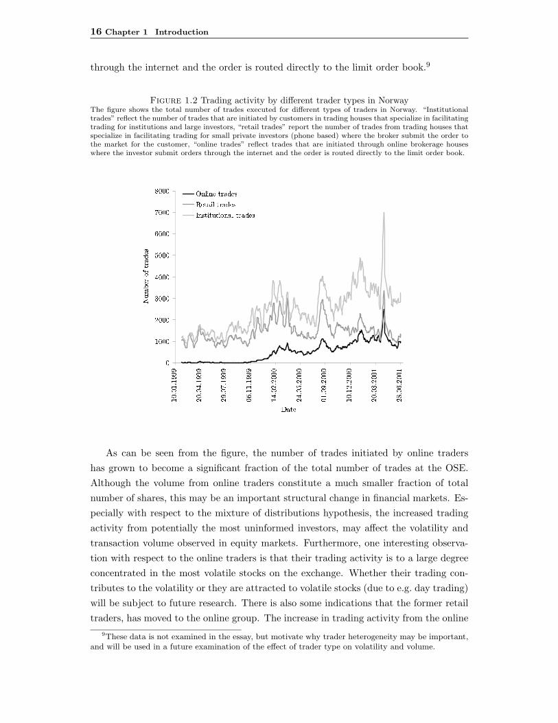
Relative to the mixture of distribution hypothesis as well as the dispersion of beliefshypothesis, one interesting trend in the Norwegian market, as in many other markets, isthat online trading has become more popular and available to investors. These systemsgenerally have much lower commissions and have given small private investors directaccess to the marketplace. To illustrate this development, figure 1.2 shows the totalnumber of trades executed in the Norwegian market that was initiated by differentgroups of trader. The type of trader is proxied by the trading house from which theinitiating order originates. “Institutional trades” reflect the number of trades in which acustomer in trading houses that mainly trade for institutional traders are the initiatingparty in the trade, “retail trades” report the number of trades from trading houses thatspecialize in facilitating trading for small private investors (phone based) where thebroker submit the order to the market for the customer, “online trades” reflect tradesthat are initiated through online brokerage houses where the investor submit orders
16 Chapter 1 Introduction
through the internet and the order is routed directly to the limit order book.9
Figure 1.2 Trading activity by different trader types in NorwayThe figure shows the total number of trades executed for different types of traders in Norway. “Institutionaltrades” reflect the number of trades that are initiated by customers in trading houses that specialize in facilitatingtrading for institutions and large investors, “retail trades” report the number of trades from trading houses thatspecialize in facilitating trading for small private investors (phone based) where the broker submit the order tothe market for the customer, “online trades” reflect trades that are initiated through online brokerage houseswhere the investor submit orders through the internet and the order is routed directly to the limit order book.
�
� �����
�������
�������
�������
�������
������
�����
�������
� �� � �� ���
� �� � �� ���
���� � �� ���
� ��� �� ���
� � � � ��
�� � � ��
� � � ��
� ��� � ��
� �� � �� �
�� � � �� �
�������
� � ! " #$% & #'( ")
*,+�- . + �/�102��3��5467�8�2� . - ��02��3��549 + 41� . ��:�� . ;�+ � - �10<��3��54
As can be seen from the figure, the number of trades initiated by online tradershas grown to become a significant fraction of the total number of trades at the OSE.Although the volume from online traders constitute a much smaller fraction of totalnumber of shares, this may be an important structural change in financial markets. Es-pecially with respect to the mixture of distributions hypothesis, the increased tradingactivity from potentially the most uninformed investors, may affect the volatility andtransaction volume observed in equity markets. Furthermore, one interesting observa-tion with respect to the online traders is that their trading activity is to a large degreeconcentrated in the most volatile stocks on the exchange. Whether their trading con-tributes to the volatility or they are attracted to volatile stocks (due to e.g. day trading)will be subject to future research. There is also some indications that the former retailtraders, has moved to the online group. The increase in trading activity from the online
9These data is not examined in the essay, but motivate why trader heterogeneity may be important,and will be used in a future examination of the effect of trader type on volatility and volume.

1.1 Introduction and overview 17
trader group may therefore partly be because retail traders has switched to this wayof trading, that online trading attract new traders to the market, or that former retailtraders trade more when it is easier and cheaper for them to execute trades. Anotherinteresting issue relating to the DBH is that the online traders may potentially be thosetraders that has the least precise information. If these traders react more frequentlyto recent order flow, they may also be the group that contributes the greatest excessvolume and excess volatility in a DBH setting. More specifically, as suggested by theDBH, the more uninformed traders, the higher the excess volatility and volume is ex-pected to be. How and whether the increase in online trading has affected the volumeand volatility in the Norwegian market, and whether this can be related to the mixtureof distributions hypothesis as well as the dispersion of beliefs hypothesis, will be subjectto further research.
1.1.2 Essays in corporate finance
One important question in corporate finance is how firms distribute profits back to theirowners. The most common way firms do this is through regular cash dividends and openmarket share repurchases. Although the most frequently studied, and historically mostcommon cash distribution, is regular cash dividends, several studies on the US marketshow that repurchases have become increasingly important over the years. Comparedto dividend distributions, an open market share repurchase is an event where the issu-ing firm trades its own stock. Thus, compared to a pro-rata dividend distribution, anon-proportional repurchase changes the ownership- and capital structure in the firm.In addition to being a more flexible payout method, a repurchase may also convey in-formation to the market about the value of the firm. However, as discussed in Bravet al. (2003), the motives behind different types of payout policy as well as recent shiftsin payout policy is not well understood. For example, Fama and French (2001) find ev-idence that dividend payments by US firms has decreased significantly over time. AlsoGrullon and Michaely (2002) find that there has been decrease in dividend paying firmsthrough time, but also find evidence that many firms substitute repurchases for divi-dends and that US firms now distribute as much cash through repurchases as throughdividends. In the study by Brav et al. (2003) they note that despite the fact that thereis a lot of research available on firms payout policy, the most fundamental issues remainsunanswered:
• Why do both dividends and repurchases exist?
• Why is there such a large penalty for dividend cuts, but no analogous penalty fornot completing a repurchase program?
In addition, there are also unresolved issues with respect to how the market responds torepurchase announcements and how repurchases may be used to e.g. signal mispricing
18 Chapter 1 Introduction
or as a mechanism for ensuring that managers don’t use excess cash to engage in valuedestroying projects and increase their private benefits.
In this second part of the thesis, I examine detailed repurchase data from Norwaywhich may cast some light on the questions mentioned above. A dominating part ofthe available empirical research on open market share repurchases is on data from theUS and Canada. The main reason for this is that repurchases has been legal in thesemarkets for several decades, while many other countries has allowed repurchases morerecently, one of which is Norway. One interesting aspect of the Norwegian repurchasedata is that firms in Norway are subject to a legal requirement to report their actualrepurchase activity immediately. Comparably, US firms are not required to report theirrepurchase activity. In Canada, the requirement is stricter than in the US as firmsare required to report their accumulated repurchases on a monthly basis. Thus, theNorwegian data may help us examine some questions in more detail that are difficultto study using aggregate data.
In contrast to the two first essays of the thesis, these two last essays relate to thetrading decisions by corporations that trade in their own stock. In addition to being away for firms to conduct their payout policy, a repurchase may also contain importantinformation since the managers of the firm potentially is the ultimate informed partici-pant in the market for its own securities. Thus, in the essays I examine how this activityrelates to asymmetric information between the firm and the market and to what extentthis information is reflected in prices. In addition, since a special feature of repurchases(compared to cash dividends) is that it changes the ownership composition of the firm,I examine whether there are systematic patterns in the ownership composition in thesefirms, and whether there are certain ownership characteristics that may constitute anunderlying motivation for why firms repurchase shares.
As summarized in Allen and Michaely (2003), there are five potential imperfectionsrelative to the Miller and Modigliani (1961) framework that may be important consid-erations when choosing dividend policy:
1 Taxes - if dividends are taxed more heavily than capital gains, minimizing divi-dends is optimal
2 Asymmetric information - if managers have private information they can use pay-out policy to signal this to the market
3 Incomplete contracts - payout policy can be used to discipline management andreduce agency costs of free cash
4 Institutional constraints - if various institutions prefer dividends, the firm mayfind it optimal to pay dividends although this imposes a tax burden on individualinvestors
1.1 Introduction and overview 19
5 Transaction costs - if dividends minimize transaction costs to equity holders, thendividend payout may be optimal.
The two essays in the last part of the thesis are related to several of these imperfec-tions. In the first essay I examine whether asymmetric information and signalling maybe an explanation for the markets reaction to the announcements of repurchase plansand the actual repurchase executions. In the last essay, the main focus is related toincomplete contracts and institutional constraints in the sense that ownership composi-tion and corporate governance may be a motivation for why firms initiate a repurchaseprogram.
Essay 3: The market impact and timing of open market share repurchases
in Norway
An emerging body of empirical literature suggests that the market underreacts to newinformation about firms’ cash flows. Public announcements that are likely to containinformation about current and future cash-flows, such as earnings surprises and dividendinitiations and omissions as well as the announcements of repurchase plans, are followedby an abnormal return drift in the same direction as the initial announcement return.This suggests that the market does not react in a complete and unbiased fashion tothis information which is inconsistent with market efficiency in its weakest form. Inother words, the direction of the price impact of the initial announcement (historicalreturns) can be used to predict future returns, using old information. Investors shouldnot be able to earn superior returns by exploiting these systematic features withoutbearing additional risk since the mispricing should be mitigated through arbitrage. Ata fundamental level, these findings may be related to misspecification of the benchmarkmodel for expected returns rather than mispricing. To explain the underreaction, theliterature suggests several reasons for why these patterns are observed. Fama (1999)argue that the empirical findings of over- and underreaction in various settings aresample specific and appear by chance. He also points to the fact that the long termabnormal return drifts are sensitive to the model specification, such that when takingaccount of size and value factors these patterns are mitigated. On the other hand, theincreasing amount of studies providing new empirical evidence on these issues, applyingdifferent model specifications and samples, suggest that alternative explanations maybe required. One strand of the literature propose behavioral models to explain theanomalies. One recent example is Barberis et al. (1998) who proposes that investorsentiment is important with respect to how investors form expectations about futureearnings, and that investors are expected to overreact and underreact to different typesof announcements due to psychological biases when interpreting new information. Otherstudies propose extensions to the existing paradigm, where additional risk factors mayhelp explain the patterns.

20 Chapter 1 Introduction
This paper examines a detailed dataset on announcements of open market sharerepurchase program announcements and actual repurchases conducted by Norwegianfirms during the period 1998-2001.10 The first purpose of the paper is to study whetherthere is an announcement effect related to when firms announce repurchase plans inNorway. In addition, the paper examines whether this initial effect is complete andunbiased relative to the long term performance of announcing firms. Essentially, themain result from this part of the analysis is that Norwegian firms also experience apositive price impact of about 2.5% when announcing a repurchase plan, in line withmodels where the market interpret the announcement as positive information aboutfuture profitability. In addition, I find that these firms show a long term abnormalperformance after the announcement of about 0.9% per month or 11% a year whencontrolling for size, book to market and momentum factors. These results line up withstudies from the US and Canada suggesting that the market reaction to the initialannouncement is incomplete with respect to the full signal value proxied by the post-announcement abnormal return.
These results contribute to the existing literature in the sense that the study addsan observation to the cross section of countries with additional evidence on the mar-ket reaction to repurchase announcements as well as the performance of these firms.However, the most interesting part of the Norwegian data is the detailed knowledgeabout the firms actual repurchases. The paper exploits this unique feature of the datato further investigate the underreaction of announcing firms and examine how the post-announcement performance relates to whether the firm actually repurchase shares ornot. More specifically, by creating two portfolios conditional on whether the firms re-purchase or not, an interesting pattern is observed. Those firms that do not repurchaseexperience a long term abnormal performance, while the portfolio of firms that actuallyrepurchase shares (and are included in a second portfolio the month after they haveconducted their first repurchase) perform as expected relative to several model specifi-cations. In addition, when examining the excess return related to actual repurchases,the results indicate that the first repurchase executed by a firm after it has announceda repurchase plan has the strongest abnormal price effect, while subsequent repurchaseshas a decreasing impact.
The paper suggests several explanations for this finding. One interpretation for thedifference in long-term abnormal performance between repurchasing and non-repurchasingfirms may be that the market reacts in a complete fashion at the announcement of theprogram for firms that later repurchase shares, while there is an underreaction fornon-repurchasing firms. This may be because the repurchasing firms are able to morecredibly signal undervaluation at the announcement of the program. However, I do
10Firms where first allowed to actually execute repurchases from 1999, but were allowed to announcethe repurchase plan earlier.

1.1 Introduction and overview 21
not find a different announcement effect for announcements that result in subsequentrepurchases relative to announcements that do not result in subsequent repurchases.
Another explanation focuses on the signal conveyed to the market when the firmchoose to actually execute a repurchase. One of the most prevalent explanations forwhy firms experience a positive price effect when announcing a repurchase plan is thesignalling hypothesis. The hypothesis assumes that there is asymmetric informationbetween the managers of the firm and the market. By announcing a repurchase plan,the manager implicitly conveys to the market that he assess the current market price tobe too low relative to the true value of the firm. However, since the announcement ofa repurchase plan is no commitment by the firm to actually repurchase any shares thesignal may be argued to be very weak.11 On the other hand since the actual repurchasesinvolves real transactions, the actual repurchases may be argued to be stronger signals ofundervaluation, or a confirmation of the initial announcement. Thus, one interpretationof the finding may be that when the firm executes its first repurchase, the market reactto the information implicit in this action, increasing the price closer to the true value,such that subsequent returns evolve as expected. When examining the price impact ofsubsequent repurchases, the results suggest that the first repurchase by a firm, has thegreatest abnormal price impact, while subsequent repurchases has a decreasing priceeffect. This may indicate that the first repurchase by a firm is the most informative inthe sense that it resolves the uncertainty with respect to whether the firm will repurchaseor not.
For the group of firms that do not repurchase there may be many reasons for whythey do not execute any repurchases. One reason may be that these firms experience aprice increase before the firm is able to execute any repurchases, such that the managerassess the firm to no longer being undervalued. An additional explanation may be thatthese firms are unable to execute repurchases simply because they are less liquid. Whenexamining measures of liquidity (quick ratio and current ratio), the results indicate thatnon-repurchasing firms are significantly less liquid than repurchasing firms. Thus, thenon-repurchasing firms may for this reason be unable to signal undervaluation throughactual repurchases. If this is the case, the price of these firms remains too low andinformation surprises in later periods contribute to the long term abnormal drift for thesecompanies. However, we cannot exclude the possibility that these firms are exposed torisks that are not captured by the market, book/market and momentum factors.
In a broader perspective, the findings relate to a concern that has been raised inthe popular press as well as by researchers in the US. It has been argued that the
11For a signal to be credible, the action must incur some costs to the manager if he signals falsely. Forexample, if the manager in addition to announcing a repurchase plan or repurchase shares commit toretaining his shares, the signal would become much stronger because he then would reduce his wealthby repurchasing at a high price. However, such commitments are rarely observed in connection to openmarket share repurchases.

22 Chapter 1 Introduction
announcement of a repurchase plan is a way for the management to raise the stockprice at little or no cost in the short run. In fact Kracher and Johnson (1997) arguethat many firms in the US announce repurchase plans with no intention of repurchasingat all. One of their arguments is that since the reporting standards in the US, withrespect to open market repurchases, are very loose, it is difficult for investors to actuallyknow whether announcing firms under normal circumstances are actually going throughwith the repurchase plan. Their main suggestion is that US firms should be requiredto report the progress of the repurchase plan such that they are motivated to onlyannounce a repurchase plan when their intentions are true.
The results in the present paper may contribute to the discussion about disclosurerequirements in the US. Although the paper does not resolve the underreaction puzzle,the results may indicate that by requiring firms to report their transactions immediatelyto the market, this may improve price discovery.
Essay 4: The ownership structure of repurchasing firms
As expressed by Schleifer and Vishny (1997);
Corporate governance deals with the ways in which suppliers of finance tocorporations assure themselves of getting a return on their investment. Howdo the suppliers of finance get managers to return some of the profits tothem? How do they make sure that managers do not steal the capital theysupply or invest in bad projects? How do suppliers of finance control man-agers?
While a dividend payment reduces the cash of the firm, a repurchase also poten-tially revises each remaining shareholder’s ownership proportion in the repurchasingfirm. Thus, in addition to being used as e.g. signal private information, as examined inthe previous essay, it may also be used by the firm to change the ownership structureof the firm or as a disciplinary mechanism when the corporate governance is weak. Forexample, in firms with potentially high agency costs of free cash (liquid firms with noprofitable investment opportunities, low concentration and low insider ownership), arepurchase may be a way to trim the cash holdings as an alternative or in addition todividends. Since a repurchase is more flexible than dividends12 it may be attractive tofirms with volatile cash flows. A repurchase may also be used by managers as an effec-tive measure against takeovers which would threaten the position of the managers, byremoving shareholders with the lowest valuations ((Bagwell, 1991)) as well as increasingthe ownership proportion of the insiders and the most loyal owners.
In a recent study, based on interviews with corporate officials, Brav et al. (2003) findthat financial executives believe that the ownership structure of their firm is important.
12Flexible in the sense that the market expects firms to keep their dividend payments at the new levelif increased (Lintner, 1956; Brav et al., 2003), and punish firms that decrease their dividend payment.
1.1 Introduction and overview 23
In addition they also believe that retail investors have a strong preference for dividends(despite a tax disadvantage) while institutional investors have no strong preferencebetween dividends and repurchases. Despite this, a large fraction of the executives(57%) stated that institutions are important with respect to establishing a repurchaseprogram. In addition, the results from the interviews suggest that payout initiationsare to a certain degree motivated by firms to avoid possible agency costs that couldoccur in the future if excess cash should accumulate within the firm. As suggested byJensen (1986), payout policy may be used as a mechanism to mitigate agency costsof free cash. Interestingly, when the executives are asked whether they would initiatepayouts to discipline themselves only 10% respond positively.13 Another interestingfinding, which relates to the previous essay, was that most executives answered thatchanges in payout policy conveyed their confidence about the firm’s future prospects.About 85% of the executives believed that repurchase decisions revealed information tothe market about mispricing.
Overall, the interviews conducted by Brav et al. (2003) provide a motivation forexamining the ownership structure of repurchasing firms. This may provide additionalevidence on the motivations for why managers initiate repurchases that are difficult toobtain through interviews such as e.g. shareholder expropriation and insider tradingaround repurchase events. An additional motivation is that there is a large empiricaland theoretical literature aimed at explain why firms repurchase shares. However, few ofthese studies examine how this relates to ownership structure and corporate governance,mainly due to the lack of detailed ownership data.
Having access to detailed monthly ownership data, for all firms listed on the OsloStock Exchange, makes it possible to conduct a detailed examination of the ownershipstructure of repurchasing firms. The ownership data contains information on the numberof shares owned by each owner as well as information with respect to the type of owners.In addition, we have data on the insider ownership in all listed firms. The essay providesan examination of the ownership structure of repurchasing firms, and tries to reconcilethese findings with available theory.
The paper finds some interesting patterns in the data. The main results indicate thatfirms that announce a repurchase plan have a significantly lower ownership concentrationthan non-announcing firms. In addition, firms that announce repurchase plans have onaverage twice as many shareholders as non announcing firms, while the size of thefirms in the two groups are similar. This would be in line with an agency theoreticalprediction that firms with dispersed ownership may be more exposed to agency problemssince there are less incentives to monitor management. Thus, if managers want toconvey to the market that they are committed to not wasting cash, the initiation of a
13As noted by Brav et al. (2003), the managers may be reluctant to admit (even to themselves) thatthey may need to be monitored or impose disciplining mechanisms on themselves.

24 Chapter 1 Introduction
repurchase plan may be one way of sending this message. In addition, firms with manysmall shareholders may want to reduce the number of shareholders to concentrate theownership and thereby reduce the probability of successful hostile takeover attemptsthat could result in the replacement of the managers. The results also indicate that theinsider ownership is much higher in announcing firms, and that the insider ownershipis the highest in firms that actually repurchase shares. With respect to the agencycost motivation, this result point in the opposite direction in the sense that agencytheory predicts that high insider ownership aligns the interests of inside- and outsideshareholders (Jensen and Meckling, 1976) such that additional mechanisms to mitigateagency costs are not needed. The high insider ownership in these firms may insteadindicate that takeover defense, outside shareholder expropriation, or entrenchment maybe reasons for why managers choose to repurchase shares.
The paper also examine how the ownership characteristics change through time whenfirms execute repurchases. As expected, the concentration increases, mainly due to anincreased ownership by the largest owner, and the number of shareholders decreases. Inaddition, the ownership of institutional and personal owners decreases, while the stateownership increases. This may be because institutional and personal investors are thosethat trade more actively in the market, and thereby are more likely to sell shares backto the firm. On the other hand the decrease may also reflect a that these two groups ofinvestors have a preference for dividend paying firms, and reduce their ownership if therepurchasing firms substitute repurchases for dividends. The reduction in institutionalownership is interesting since a study by Grinstein and Michaely (2001) find an oppositetrend in the US. They argue that firms attract institutions through their payout policy,and find that institutions increase their holding in repurchasing firms.
The final part of the study applies a binary regression method to examine whetherthe ownership at the beginning of each sample year can explain the propensity for firmsto initiate a repurchase program. The findings is similar to the descriptive part ofthe study, but some additional results appear. First, insider ownership increases theprobability of announcement, while concentration is insignificant for all years. However,the existence of a large controlling shareholder reduces the propensity to announce,while the identity of the largest shareholder is unimportant. In addition, the resultsstrongly suggest that firms that paid dividends in the previous year, are less likely toinitiate a repurchase program, while larger firms are more likely to announce repurchaseplans. This is probably related to dividend smoothing, and that firms are reluctant tocutting dividends as suggested in studies by Lintner (1956) and Brav et al. (2003). Inaddition, large firms often has a higher number of small shareholders, which may be onemotivation for these firms to initiate a repurchase program.
Overall, although the findings in the paper does not strongly favor one interpretationover the other, the results are in line with an interpretation where insiders have incen-

1.1 Introduction and overview 25
tives to support the initiation of a repurchase program either to maximize the futurevalue of their wealth (Isagawa, 2000), expropriate outside shareholders or to entrenchthemselves. On the other hand the finding that a controlling shareholder decreases theprobability of observing an announcement, may also suggest that controlling sharehold-ers oppose the initiation of a repurchase program. Alternatively, a large shareholdermay have stronger incentives to monitor, such that an additional mechanism to re-duce agency costs of free cash is not needed. Interestingly, this finding is the oppositeof what is the prediction in the model by Brennan and Thakor (1990) where, largeshareholders prefer repurchases to dividends, while small shareholders prefer dividends.Thus, relative to their model, one would expect large shareholders to increase the firmspropensity to initiate a repurchase program since they would use their voting rights toforce a repurchase plan into place.
Future research on repurchases
The two essays on open market share repurchases provide some interesting results bothwith respect to the announcement effect, the underreaction hypothesis, the price effectof actual repurchases as well as on the ownership structure in repurchasing firms. Al-though, the two essays are separated in this thesis, they may be linked in several ways,which may motivate future research on this topic.
First, a critical question with respect to the signalling ability of open market re-purchase announcements is whether the announcement is a credible signal. As will bediscussed in chapters 4 and 5, relative to the signaling hypothesis the announcementof an open market share repurchase plan is not a commitment by the firm to actuallyrepurchase any shares, neither does it impose any cost on the manager of the firm ifit is a false signal aimed at temporarily increasing the stock price. As suggested byIsagawa (2000), the announcement of a repurchase plan may be credible if the managerhas a stake in the firm through stock ownership or options, such that his future wealthdepends on the value of the firm. In that case the announcement of a repurchase plan,as well as repurchase executions, signals information about the private benefits for themanager to indulge in suboptimal investments. If the private benefit from using cash onnegative net present value projects is lower than his benefit from increasing the valueof the firm, he will support the initiation of a repurchase program as well as executerepurchases instead of wasting cash that would lower the value of the firm and his ownwealth. Thus, future research may try to examine more closely the relationship betweenthe ownership composition in firms as well as how this relates to the signalling effect ofrepurchase announcements, and the future value of the firm.
A related issue which is not studied in the repurchase essays is whether the re-purchase executions that are observed ex post were intended ex ante. In other words,firm specific or market wide events occurring after the announcement of the program
26 Chapter 1 Introduction
may change the motivation for why firms in general execute repurchases. One exampleare large negative market movements that induce firms to repurchase to e.g. stabilizetheir stock prices. On recent example was the large drop in prices after the terroristattacks in the US in 2001 which spurred a huge increase in the initiation of repurchaseprograms as well as actual repurchases. Although the huge increase in repurchases dur-ing this period was partly due to the Securities and Exchange Commission suspendingregulations with respect to daily volume restrictions on repurchases, similar bursts inrepurchase activity is found for Norway as well. In addition, findings in other studies(Stephens and Weisbach, 1998) suggest that negative price movements seem to triggerrepurchases. However, more interestingly, firm specific events which were not antici-pated by the managers at the announcement date may also affect whether the firm gothrough with repurchases or not. This is an important and interesting issue since an-nouncing firms are likely to “self select” into being repurchasers or non-repurchasers. Inthe paper I find that the time between the announcement of the program and the initialrepurchase executed by the firm is on average about 200 days (median 169 days). Thisindicates that the initiation of the program is not intended for immediate use, but ratherto provide an option to the managers to execute repurchases when the circumstancesare favorable or help provide liquidity to the marketplace. On the other hand, somefirms execute repurchases very soon after the program announcement while about 40%of the firms do not repurchase at all. Thus, an interesting extension of the project wouldbe to try to model the repurchase decision after the announcement of the repurchaseprograms to determine what are the main decision variables.
Second, several studies suggest that ownership structure may be important for eco-nomic performance and the value of the firm. Although the empirical results on thisissue are ambiguous, several studies find that ownership structure matters for economicperformance. In a study for the Norwegian market, Bøhren and Ødegaard (2001) findthat insider ownership creates value while ownership concentration destroys value. Thus,if open market repurchases change the ownership composition in firms, or firms withcertain ownership constellations are more likely to initiate repurchase programs, thismay be important for the economic performance of these firms.
A final research topic with respect to repurchases relates the two last papers tomicrostructure issues. As suggested by Barclay and Smith (1988), the initiation ofa repurchase program may increase the spread in the market since the probability oftrading with an informed investor increases. Initially, this may be related to a higherprobability of trading with the firm itself which increases the adverse selection compo-nent of the spread. An interesting topic for future research would be to combine thedetailed intraday data used in chapter 3 with the data used in the two last essays toexamine whether there is a effect on the adverse selection component of the spread aftera firm announces a repurchase plan. In addition, it may be possible to track the actual

1.1 Introduction and overview 27
repurchase executions in the intraday data to examine in more detail how the marketreacts to the trading activity of an potentially informed trader, the firm.

28 Chapter 1 Introduction
Bibliography
Allen, F. and Michaely, R. (2003). Payout Policy, in Handbooks of the Economics ofFinance, volume 1A, chapter 7, pages 337–429. Elsevier.
Bagwell, L. (1991). Share repurchases and takeover deterrence. RAND Journal ofEconomics, 22:72–88.
Barberis, N., Schleifer, A., and Vishny, R. (1998). A model of investor sentiment.Journal of Financial Economics, 49:307–343.
Barclay, M. J. and Smith, C. W. (1988). Corporate payout policy. Journal of FinancialEconomics, 22:61–82.
Bessembinder, H. and Seguin, P. (1993). Price volatility, trading volume, and mar-ket depth: Evidence from futures markets. Journal of Financial and QuantitativeAnalysis, 28(1):21–39.
Biais, B., Hillion, P., and Spatt, C. (1995). An empirical analysis of the limit orderbook and the order flow in the Paris Bourse. Journal of Finance, 50:213–231.
Bøhren, Ø. B. and Ødegaard, B. A. (2001). Corporate governance and economic per-formance: A closer look. Working paper, Norwegian School of Management (BI).
Brav, A., Graham, J. R., Harvey, C. R., and Michaely, R. (2003). Payout policy in the21st century. NBER Working Paper No.9657.
Brennan, M. J. and Thakor, A. V. (1990). Shareholder preferences and dividend policy.Journal of Finance, 45:993–1018.
Clark, P. (1973). A subordinated stochastic process model with finite variance forspeculative prices. Econometrica, 41:135–155.
Conrad, J., Johnson, K. M., and Wahal, S. (2001a). Institutional trading and softdollars. Journal of Finance, 56:397–416.
Conrad, J., Johnson, K. M., and Wahal, S. (2001b). Institutional trading costs andalternative trading systems. Working Paper, University of North Carolina at ChapelHill, Forthcoming in Journal of Financial Economics.
Daigler, R. and Wiley, M. (1999). The impact of trader type on the futures volatility-volume relation. Journal of Finance, 54:2297–2316.
Easley, D., Kiefer, N. M., and O’Hara, M. (1996). Cream-skimming or profit sharing?The curious role of purchased order flow. Journal of Finance, 51:811–833.
Fama, E. F. (1999). Market efficiency, long-term returns, and behavioural finance.Journal of Financial Economics, 49:283–306.
Fama, E. F. and French, K. R. (2001). Dissappearing dividends: changing firm charac-teristics or lower propensity to pay? Journal of Financial Economics, 60:3–43.
Fong, K., Madhavan, A., and Swan, P. (1999). Why do securities markets fragment?Working Paper, University of Southern California.

BIBLIOGRAPHY 29
French, K. and Roll, R. (1986). Stock return variances. the arrival of information andthe reaction of traders. Journal of Financial Economics, 17:5–26.
Ghysels, E. and Juergens, J. L. (2001). Stock market fundamentals and heterogeneityof beliefs: tests based on a decomposing of returns and volatility. Unpublished paper,University of North Carolina.
Grinstein, Y. and Michaely, R. (2001). Institutional holdings and payout policy. WorkingPaper, Cornell University.
Grullon, G. and Michaely, R. (2002). Dividends, share repurchases, and the substitutionhypothesis. Journal of Finance, 57:1649–1684.
Harris, L. (1987). Transaction data tests of the mixture of distributions hypothesis.Journal of Financial and Quantitative Analysis, 22(2):127–141.
Harris, L. (2003). Trading and Exchanges. Market Microstructure for Practitioners.Oxford University Press.
Hendershott, T. and Mendelson, H. (2000). Crossing networks and dealer markets:Competition and performance. Journal of Finance, 55:2071–2115.
Isagawa, N. (2000). Open-market stock repurchase and stock price behavior when man-agement values real investment. The Financial Review, 35:95–108.
Jensen, M. C. (1986). Agency costs of free cash flow, corporate finance, and takeovers.American Economic Review, 76:323–329.
Jensen, M. C. and Meckling, W. H. (1976). Theory of the firm: Managerial behavior,agency costs and capital structure. Journal of Financial Economics, 3:305–360.
Jones, C. M. and Lipson, M. L. (1999a). Execution costs of institutional equity orders.Journal of Financial Intermediation, 8:123–140.
Jones, C. M. and Lipson, M. L. (1999b). Sixteenths: Direct evidence on institutionalexecution costs. Working Paper, Columbia Business School.
Keim, D. B. and Madhavan, A. (1995). Anatomy of the trading process: Empiricalevidence for the motivation for and execution of instituional equity trades. Journalof Financial Economics, 37:371–398.
Keim, D. B. and Madhavan, A. (1997). Transactions costs and investment style: Aninter-exchange analysis of institutional equity trades. Journal of Financial Economics,46:265–292.
Kracher, B. and Johnson, R. R. (1997). Repurchase announcements, lies and falsesignals. Journal of Business Ethics, 16:1677–1685.
Lintner, J. (1956). Distribution of incomes of corporations among dividends, retainedearnings, and taxes. American Economic Review, 46:97–113.
Madhavan, A. (1995). Consolidataion, fragmentation, and the disclosure of tradinginformation. Review of Financial Studies, 8:579–603.

30 Chapter 1 Introduction
Madhavan, A. (2000). Market microstructure: A survey. Journal of Financial Markets,3:205–258.
Miller, M. and Modigliani, F. (1961). Dividend policy, growth, and the valuation ofshares. The Journal of Business, 34:411–433.
Schleifer, A. and Vishny, R. W. (1997). A survey of corporate governance. Journal ofFinance, 52:737–783.
Shalen, C. (1993). Volume, volatility, and the dispersion of beliefs. Review of FinancialStudies, 6(2):405–434.
Shiller, R. (1981). Do stock prices move too much to be justified by subsequent changesin dividends? American Economic Review, 71(3):421–436.
Stephens, C. P. and Weisbach, M. S. (1998). Actual share reacquisitions in open marketrepurchase programs. Journal of Finance, 53:313–333.
Chapter 2
Equity Trading by Institutional
Investors: Evidence on Order
Submission Strategies
Written with Randi Næs 1
Abstract
The trading volume channelled through off-market crossing networks is growing.Passive matching of orders outside the primary market lowers several componentsof execution costs compared to regular trading. On the other hand, the risk of non-execution imposes opportunity costs, and the inherent “free riding” on the pricediscovery process raises concerns that this eventually will lead to lower liquidityin the primary market. Using a detailed data set from a large investor in the USequity markets, we find evidence that competition from crossing networks is con-centrated in the most liquid stocks in a sample of the largest companies in the US.Simulations of alternative trading strategies indicate that the investor’s strategy ofinitially trying to cross all stocks was cost effective: in spite of their high liquidity,the crossed stocks would have been unlikely to achieve at lower execution costs inthe open market.
1The article is published in Journal of Banking & Finance 27 (2003) 1779-1817.
31
32 Chapter 2 Equity Trading by Institutional Investors
2.1 Introduction
There is currently a plethora of venues for trading US equities. Some fit the needs ofsmall retail investors while others are more suited for the needs of large institutionalinvestors and portfolio managers.2 Using a detailed data set from a large institutionalinvestor, we investigate the nature of competition between a principal exchange andone particular type of alternative trading system, the crossing network. A crossingnetwork is a satellite trading place: it uses prices from the primary market and merelymatches quantities. Passive matching of orders implies that several components ofexecution costs are low compared to regular market trading: commissions are lower andthere are no spread costs or direct price impact costs. On the other hand, traders arenot guaranteed execution in the network, and this may lead to significant opportunitycosts. In addition, the execution probability may or may not be associated with adverseselection costs, depending on the type of traders in the crossing network.3 Finally,because crossing networks compete for order flow, crossing participants may eventuallyincur implicit price impact costs as a result of reduced primary market liquidity. Thelargest crossing markets in the US include POSIT (ITG), NYSE crossing session I andII, and Instinet Global Crossing. In addition, there are less public internal crossingnetworks, many of which are the exclusive domains of institutional investors.4
Investigating execution costs associated with different trading methods is of obviousinterest to investors seeking cost effective ways to trade. However, the functioning ofalternative trading systems should also be of interest to academics, regulators and policymakers responsible for the design of securities markets. The recent success of electronic
2The trading venues can be broadly classified into four groups: (i) the principal exchanges, (ii) the“over the counter” (OTC) markets, (iii) other exchanges and (iv) alternative trading systems (ATS).The principal exchanges include the NYSE and the NASDAQ/NNM. The OTC markets includes theOTC bulletin board and the ”pink sheet” market. The OTC bulletin board is for companies too small tolist on the NNM, and the ”pink sheet” market is an internet quotation service for very small companiesoperated by Pink Sheets LLC. Other exchanges include the AMEX, the regional exchanges in Boston,Philadelphia, Pacific, and Chicago(Midwest), and the Cincinnati Stock Exchange. Finally the ATSsinclude Electronic Communication Networks (ECNs), the Arizona Stock Exchange, and external andinternal crossing networks.
3A stated goal of many crossing networks is to keep the identities and trades of their participantsanonymous, both before and after the trades. The following example is taken from the Instinet home-page: ”With Instinet Global Crossing, the process is anonymous. Pre-trade or post-trade, neither yourtrading partner nor other market participants will know your identity, strategy, order size, or residualsize.”
4POSIT is by far the largest crossing market and facilitated the crossing of 7.8 billion shares in 2000and 9.3 billion shares in 2001. POSIT performs eight daily matches at the price equal to the bid-askmidpoint of the stock’s primary market at fixed times which are randomized within 5 minutes to avoidmanipulation. The NYSE after hours crossing session I allows participants to submit orders until 5pmwhen the orders are matched using the NYSE closing price for each stock. The NYSE crossing sessionII is designed to facilitate trading of baskets of at least 15 NYSE securities valued at USD 1 million ormore. Instinet Global Crossing began in 1986 as the first electronic crossing service in the US. Currently,its operations facilitate “end-of-day crossing” and “VWAP crossing”. The “end-of-day crossing” crossesorders at the closing price in the primary market, while the “VWAP crossing” is settled before theopening of the primary market and the participants are guaranteed the VWAP price during the day.
2.1 Introduction 33
trading venues has intensified the competition for order flow faced by the traditionalmarkets. In general, the increase in competition is positive because it lowers executioncosts. Several empirical studies find that transaction costs decreased over the recentpast.5 However, increased competition for order flow has also raised some concernsrelated to potentially negative effects from market fragmentation. Mendelson (1987)shows that market fragmentation has both costs and benefits. The costs are related toreduced liquidity and increased volatility in each “sub-market”, while the benefits arerelated to increased quality of the market price signals. Because crossing networks donot contribute to price discovery, the potential benefits from better price signals are lostand only the potential costs from low liquidity and high volatility are left. These costsmight also eventually harm participants in crossing networks through their relianceon primary market prices. A better understanding of the nature of the competitionbetween crossing networks and primary markets is clearly called for, including underwhat circumstances and for which types of assets crossing networks will coexist withother markets.
Three recent empirical papers on alternative trading systems are Fong et al. (1999),Næs and Ødegaard (2000), and Conrad et al. (2001b). Fong et al. (1999) use detaileddata from the Australian stock exchange (ASX) to study the competition betweenexchanges and different off-market trading mechanisms, including crossing networks(POSIT Australia). Off-market trading is found to be concentrated in the most liquidstocks. The cross-sectional differences in off-market trading seem to be driven by in-stitutional trading interest (trading volume, index inclusion), primary market liquidity(spreads, market depth, introduction of closing auction market), and the existence ofa derivative market. Conrad et al. (2001b) study explicit and implicit execution costson externally crossed orders, orders sent to ECNs, and broker-filled orders based ona large data set from the US equity market provided by the Plexus Group.6 Conradet al. (2001b) also find that the most liquid stocks are the ones underlying the orderssent to external crossing systems. Moreover, the average total trade cost is found tobe substantially lower for orders sent to external crossing systems and ECNs than fororders filled by traditional brokers.
Both papers suggest that crossing networks provide significant competition for orderflow, especially in highly liquid stocks, and considerably lower execution costs than othertrading methods. On the other hand, as hypothesized in Keim and Madhavan (1998)and Hendershott and Mendelson (2000), informed traders may be present in crossingnetworks, offsetting their explicit cost advantage. The existence of adverse selectioncosts is hard to detect based on the cost measures used in the empirical literature andthe data typically available to researchers, such as the data from the Plexus Group
5For a survey on research on transaction costs, see Keim and Madhavan (1998).6The sample consist of 797,068 orders submitted by 59 institutions between the first quarter of 1996
and the first quarter of 1998.
34 Chapter 2 Equity Trading by Institutional Investors
used in Conrad et al. (2001b). Using a special data set, the relation between executionprobability and adverse selection is studied in Næs and Ødegaard (2000). They findthat, over the month following an attempt at crossing, there is a one percent differencein risk adjusted returns between stocks that were successfully crossed and stocks thathad to be purchased in the market. This finding is interpreted as evidence that thebenefits of lower costs in crossing networks are mitigated by costs related to adverseselection.
In this paper, we extend the analysis of Næs and Ødegaard using the same data set.The data set includes all orders from the establishment of a US equity portfolio worthUSD 1.76 billion over a 6-month period from January 1998 to June 1998. The portfoliowas tracking the US part of the FTSE All World index7, which consists of about 500stocks, and has a very high correlation with the S&P 500 index. The data set is uniquein that it contains information on the investors’ complete order submission strategy,including the ex ante trading strategy, the dates on which the decision to trade wasmade, and the resulting fill rates of each order for different trading venues. Hence, thedata set is close to a “controlled experiment” which is quite rare.8 The weakness of thedata set is that it is from one trader’s buy orders only and covers a limited period oftime. Both Fong et al. (1999) and Conrad et al. (2001b) have access to huge data setson orders and trades and their results are therefore more robust than ours. However,we show that the investor in our study is quite representative for large institutionalinvestors in the US markets.
First, we try to investigate the evidence of adverse selection more closely. On theone hand, the available empirical evidence suggest that crossing networks are competingin the most liquid stocks. If stocks that are not supplied in crossing networks are lessliquid in general, then these stocks may require a higher return to induce investors tohold them, and the abnormal performance of the non-crossed stocks found in Næs andØdegaard (2000) might be explained (or partly explained) by a liquidity premium.9 Onthe other hand, a liquidity and an information story need not be mutually exclusive.First, in addition to being a proxy for differences in liquidity, a wider spread may alsocapture a higher adverse selection component. Furthermore, other measures of liquidity,such as depth, may also capture the effect that uninformed investors withdraw from themarket if they are worried about being picked off by better informed investors. Thus, adifference in liquidity between the two groups of stocks may capture the same effect as
7The FTSE All-World index includes 49 different countries and about 2300 stocks. The aim of theindex is to capture up to 90% of the investible market capitalization of each country.
8In many other studies, the exact investment strategy of a trader has to be estimated from thesequence of trades. This induces a selection bias in the data. It might be that the trader has decidedto send the most difficult orders to brokers and the least difficult orders to crossing networks. We arenot facing a selection bias problem in our data set.
9Amihud and Mendelson (1986) show that risk-adjusted returns for stocks and bonds are increasingin their illiquidity, where liquidity is proxied by the spread.
2.1 Introduction 35
found in Næs and Ødegaard (2000), but by using different proxies for adverse selection.An interesting question in this respect, is whether the liquidity characteristics are tem-porary or more systematic over time. Because information asymmetries are expected tovanish relatively quickly, it would be harder to interpret a systematic liquidity differenceas a sign of adverse selection, especially for the largest companies in the US market. Onthe other hand liquidity differences may be more permanent in nature.
We investigate these questions by calculating a whole range of liquidity and activitymeasures in the primary market across the groups of stocks that were supplied/notsupplied in the crossing network.10 Our results indicate that the difference in abnormalreturn between the two groups of stocks may be explained by both liquidity differencesand private information. On the one hand, we find support for the earlier finding thatcrossing networks are competing in the very liquid segment of listed US equities. Stocksthat are successfully crossed are significantly more liquid and more actively traded inthe primary market than stocks that are not crossed. Moreover, we also show thatthe differences in liquidity and activity between the two groups of stocks are not datespecific, but rather systematic throughout the entire period examined. On the otherhand, the difference in spread between the groups of stocks is sometimes significanteven though the measures of activity are equal. Following Easley et al. (1996b), thisis evidence of informed trading in the stocks that could not be crossed. In addition,we show that the stocks in our sample have a very high correlation with the S&P 500index. It is hard to believe that liquidity differences between the 500 largest and mostliquid companies in the US can explain a difference in abnormal performance betweenthe two groups of stocks of 1 percent over 20 days.
Second, we want to investigate the costs of following alternative submission strate-gies. This is done by simulating the set of equilibrium order submission strategies forliquidity traders in the Hendershott and Mendelson (2000) model. Our simulated strate-gies are based on real historical price/volume paths of the stocks traded. This is possibleto do because we know the dates when the decision to trade was made in addition tothe desired quantities. The simulations confirm the result that crossed and non-crossedstocks have different liquidity characteristics. The stocks that are not obtained throughcrossing are also the most difficult and expensive stocks to acquire in the market. Moreinterestingly, we find that the actual crossing strategy was inexpensive. Even thoughthe crossed stocks were among the most liquid stocks on the NYSE, it would have beenvery hard to achieve lower execution costs by submitting limit orders for the same stockson the same dates that they were first tried to be crossed.
The paper is organized as follows. In section 2.2, we describe our data set. Wefirst give a short description of the investor and the crossing strategy. Then we providesome descriptive statistics establishing that the investor is indeed representative for the
10We use the crossing success of the Fund as a proxy for supply in the crossing network.
36 Chapter 2 Equity Trading by Institutional Investors
group of large institutional traders in the US equity market. In section 2.3, we discussthe relationship between execution probability and several measures of primary marketliquidity. Section 2.4 contains a description of the methodology and results from thesimulation approach. Section 2.5 provides our conclusions.
2.2 The data
Our data set contains transactions data from an actual submission strategy carried out inthe US equities market by a large institutional investor, the Government Petroleum Fundin Norway (hereafter “the Fund”). To construct liquidity measures and simulate othersubmission strategies, we use additional transaction data from the NYSE Trades andQuotes database (TAQ), which contains all the trades and quotes for stocks listed on theNYSE, American Stock Exchange (AMEX) and NASDAQ’s National Market System.In this section, we first give a short description of the Fund and explain the opportunis-tic crossing strategy in some more detail. We then provide some descriptive statisticsto establish that the Fund is representative for the group of large institutional tradersin the US equity market.
2.2.1 The trading strategy
The Fund is a vehicle for investing the Norwegian Government’s income from petroleum-related activities in international capital markets. Initially, the Fund was invested inforeign government securities only. However, new criteria, applying from January 1998,stated that between 30 and 50 percent of the Fund portfolio was to be invested inequities. The composition of the Fund portfolio was changed to include equities duringthe first half of 1998. We use transaction data for the part of the portfolio that wasinvested in US equities during this “buildup”/transition period.
The investment universe for the equity portfolio includes at present 28 countries inEurope, America, and Asia. US stocks represent around 29 percent of the total stockportfolio. Benchmark portfolios consist of the companies in the FTSE All-World indexfor these countries.11 The US part of the index currently consists of about 480 differentsecurities. The constituents of this index are the largest companies in the US market,and the index has a very high correlation with the S&P 500 index.
The equity portion of the total benchmark portfolio was set to 8 percent at the endof January 1998, and was then increased by another 8 percentage points at the end ofeach subsequent month until it reached the benchmark weight of 40 percent in June.The maximum tracking error restriction implied that the Fund was pre-committed tobuy most of the stocks in the index every month.
11These indices used to be called the FT/S&P’s Actuaries World Index.
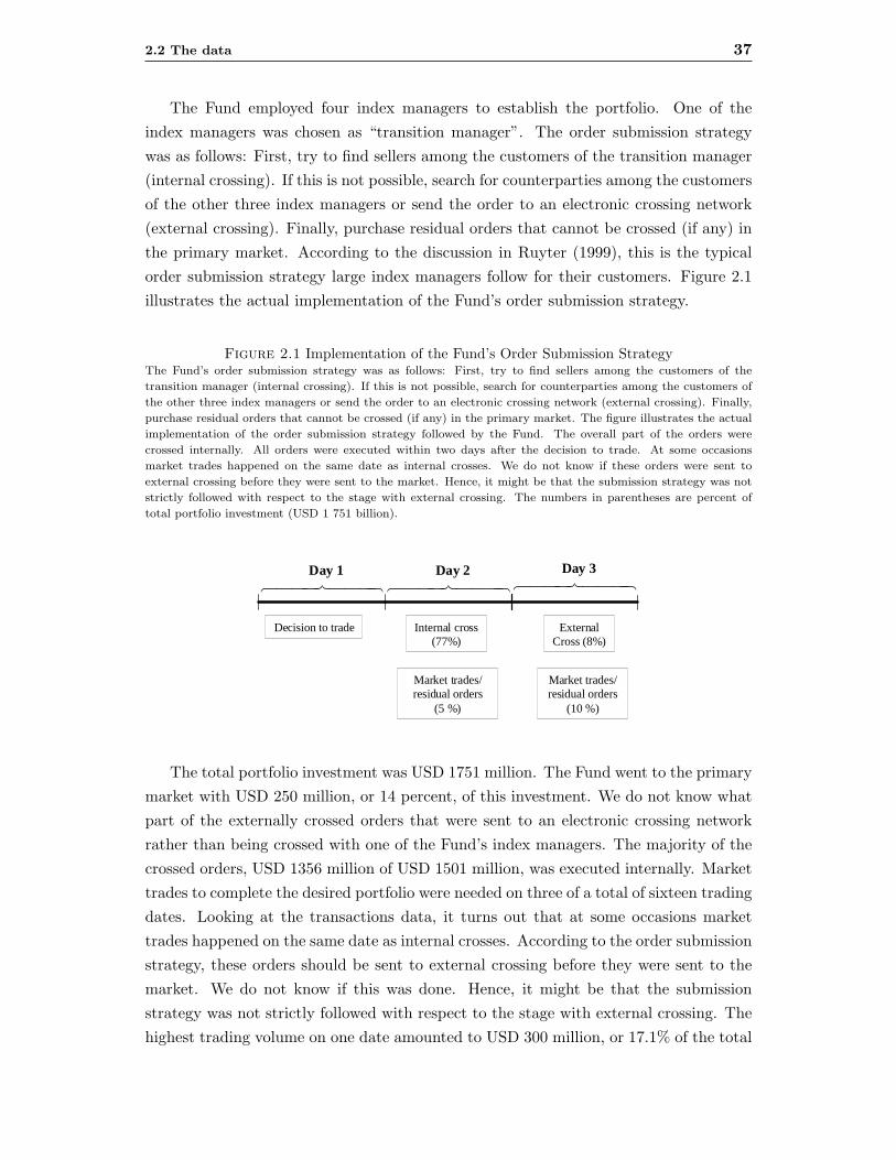
2.2 The data 37
The Fund employed four index managers to establish the portfolio. One of theindex managers was chosen as “transition manager”. The order submission strategywas as follows: First, try to find sellers among the customers of the transition manager(internal crossing). If this is not possible, search for counterparties among the customersof the other three index managers or send the order to an electronic crossing network(external crossing). Finally, purchase residual orders that cannot be crossed (if any) inthe primary market. According to the discussion in Ruyter (1999), this is the typicalorder submission strategy large index managers follow for their customers. Figure 2.1illustrates the actual implementation of the Fund’s order submission strategy.
Figure 2.1 Implementation of the Fund’s Order Submission StrategyThe Fund’s order submission strategy was as follows: First, try to find sellers among the customers of the
transition manager (internal crossing). If this is not possible, search for counterparties among the customers of
the other three index managers or send the order to an electronic crossing network (external crossing). Finally,
purchase residual orders that cannot be crossed (if any) in the primary market. The figure illustrates the actual
implementation of the order submission strategy followed by the Fund. The overall part of the orders were
crossed internally. All orders were executed within two days after the decision to trade. At some occasions
market trades happened on the same date as internal crosses. We do not know if these orders were sent to
external crossing before they were sent to the market. Hence, it might be that the submission strategy was not
strictly followed with respect to the stage with external crossing. The numbers in parentheses are percent of
total portfolio investment (USD 1 751 billion).
Decision to trade
Day 1
Internal cross(77%)
ExternalCross (8%)
444 8444 76444 8444 76 444 8444 76
Day 2 Day 3
Market trades/residual orders
(10 %)
Market trades/residual orders
(5 %)
The total portfolio investment was USD 1751 million. The Fund went to the primarymarket with USD 250 million, or 14 percent, of this investment. We do not know whatpart of the externally crossed orders that were sent to an electronic crossing networkrather than being crossed with one of the Fund’s index managers. The majority of thecrossed orders, USD 1356 million of USD 1501 million, was executed internally. Markettrades to complete the desired portfolio were needed on three of a total of sixteen tradingdates. Looking at the transactions data, it turns out that at some occasions markettrades happened on the same date as internal crosses. According to the order submissionstrategy, these orders should be sent to external crossing before they were sent to themarket. We do not know if this was done. Hence, it might be that the submissionstrategy was not strictly followed with respect to the stage with external crossing. Thehighest trading volume on one date amounted to USD 300 million, or 17.1% of the total
38 Chapter 2 Equity Trading by Institutional Investors
portfolio investment. Note that for the period we are considering the Fund was onlybuying, not selling securities. For the first two months, crossing prices were set as theprimary market (NYSE/NASDAQ) closing prices that day. For the remainder of theperiod, prices were set as the volume weighted average price (VWAP) of trades in theprimary market during the day.
2.2.2 Robustness
Our study is based on the trades of only one institution. It is therefore of crucialimportance that the investor is representative for the group of institutional investorsused in other studies dealing with similar issues.
The Fund used Barclay Global Investor (BGI) as a transition manager. Accordingto Harris (2002), BGI’s internal crossing network is “probably the largest in the world”.Hence, both the manager and the private network, where most of the actual crossingwas performed, are representative for the US market.
Most recent empirical studies of institutional investors’ in the US equity market usedata provided by the Plexus Group. These studies include Keim and Madhavan (1995,1997), Jones and Lipson (1999a,b) and Conrad et al. (2001a,b). The Plexus Group isa consulting firm that monitors the costs of institutional trading. The data sets usedin Jones and Lipson (1999a,b) are limited to trades executed in some specific firms.The most relevant samples of institutional investors with which to compare the Fund’strades are therefore the ones used in Keim and Madhavan (1995, 1997) and Conradet al. (2001b).
Keim and Madhavan (1995, 1997) use data on all equity transactions of 21 insti-tutional investors from January 1991 through March 1993. This data set contains atotal of 62,333 orders. The institutions vary in size. For fundamental value managers,the mean dollar value of assets under management was USD 4.8 billion, ranging froma low of USD 0.7 billion to a high of USD 12.9 billion. For index managers and tech-nical traders, the mean dollar value of assets under management was USD 3.2 billionand USD 5.3 billion respectively.12 In the period we are examining, the Fund was anindex tracker, and, at the end of June 1998, the US equity portfolio was worth USD 1.7billion. Conrad et al. (2001b) have a larger data set from a more recent time period.Their sample consists of 797,068 orders submitted by 59 institutions between the firstquarter of 1996 and the first quarter of 1998.
If we first look at order size, our median order is for USD 174,000. As table 2.1 shows,this is slightly larger than the median buy order of USD 138,000 in Keim and Madhavan(1995, 1997), and much larger than the crossed and ECN filled orders in Conrad et al.
12Fundamental value managers are defined as managers whose investment strategies are based on as-sessment of long-term fundamental values, technical managers are defined as managers whose strategiesare based on capturing short-term price movements, and index managers are defined as managers whoseek to mimic the returns of particular stock indexes (Keim and Madhavan, 1997).

2.3 Execution probability and primary market liquidity 39
Table 2.1Descriptive statistics for traded securities
In this table, we make a comparison of the data used in this study and in Keim and Madhavan (1995, 1997) and
Conrad et al. (2001b). In our study and in Keim and Madhavan (1995,1997), the numbers are for buyer-initiated
trades only. “Multiple mechanism orders” in the Conrad et al. (2001b) paper are orders in which more than one
of the three trading mechanisms (brokers, ECNs or external crossing systems) are used to fill the order. Market
cap values are in USD billion. “Listed%” is the percentage of total orders that is in listed stocks. “n” is the total
number of orders.
Order size LiquidityDollar value No. of shares Market cap Listed n
mean med. mean med. mean med. %Our studyAll orders 386 174 6 898 3 800 16.9 7.5 100 4 200- Cross 396 177 7 013 3 800 17.6 7.8 100 3 494- Market order 339 157 6 329 3 550 13.6 6.1 100 706
KM [1995,1997]All orders 138 4 800 1.1 82.6 36 590
Conrad et al. (2001b)All orders 723 998- External cross 187 45 12.8 >90.0 112 159- ECN’s 194 53 3.0 51 127- Broker filled 1474 137 11.1 560 712
(2001b). One of the reasons for this may be that the orders routed through ECNsare generally much smaller than orders routed through crossing networks. The averagedollar value of the Fund’s orders of USD 386,000 is also higher than the average dollarvalue of the orders sent to external crossing and ECNs, but considerably lower than theaverage dollar value of the orders filled by brokers and multiple order mechanisms.
Since the Fund was tracking the US stocks included in the FTSE All-World index,the stocks in the sample are obviously the more liquid stocks in the market. The mostliquid stocks in Conrad et al.’s study are the ones underlying the orders sent to externalcrossing systems. These securities have an average market cap of USD 12.7 billion,while the average market cap for the stocks purchased by the Fund was USD 16.9billion. Hence, the Fund was clearly trading in the larger companies.
One more characteristic with our data set is worth noting. Unlike most other studies,there is no selection bias in our data set. The Fund did not select what orders to sendto the crossing network and what orders to send to the market based on a perceptionof trade difficulty.
2.3 Execution probability and primary market liquidity
In this section, we analyze in detail the relation between the probability of getting astock crossed and the liquidity and trading activity in the primary market. This ispossible because we know that the Fund initially tried to cross all the stocks. The data
40 Chapter 2 Equity Trading by Institutional Investors
set therefore reveals the date and identity of stocks that could not be crossed. Using achoice theoretic (probit) model on the probability of seeing a stock being crossed, Næsand Ødegaard (2000) find some evidence that the crossing network is removing tradingvolume from the primary market. However, in their model, market liquidity is onlycaptured by company market values. This is not a particularly informative proxy forliquidity in our case, since all the stocks in the sample are relatively large.
We find that there are indeed significant differences in liquidity and activity betweenthe two groups of stocks based on a wide range of liquidity and activity measures.Moreover, most of the liquidity and activity measures we calculate are significantlydifferent across the groups of stocks, both on the days when they were first crossed andfor the month prior to and after the actual trading dates. These results are confirmedin a probit model. After a proper orthogonalization of the independent variables, theprobability of a successful cross is shown to be higher the lower the effective spread,the higher the liquidity ratio, and the higher the dollar trading volume in the primarymarket.
2.3.1 Liquidity measures
Market liquidity is a comprehensive concept that covers several transactional propertiesof the marketplace. Harris (1990) defines four interrelated dimensions of the concept:width, depth, immediacy and resiliency. Width is defined as the bid-ask spread for agiven number of shares, and measures the cost per share of liquidity. Depth is definedas the number of shares at the bid-ask quotes, immediacy describes how fast a trade fora given number of shares can be executed, and resiliency describes how fast the pricereverts to its ”true” value after order flow imbalances caused by liquidity trading thathas moved prices temporarily away from the ”true” level. We try to capture the width,depth and resiliency dimensions by calculating several spread, volume, and volatilitymeasures.13
Spread measures We consider three measures of the spread to capture the width ofthe market. The most commonly used spread measure is the quoted dollar spread. Itmeasures the average difference between the inside quoted ask and bid for a stock overthe trading day and can be thought of as the absolute ”round trip” cost of trading a smallamount of shares at the inner quotes. The quoted percentage spread is calculated as thequoted spread relative to the spread midpoint, or the ”true” value, at each trade time.The effective spread takes into account the fact that trades are often executed inside(price improvement) or outside the spread (”walking the book”), and is often considereda more appropriate measure of trading costs than are quoted spreads, especially for large
13A discussion of data issues and the formulas for calculating the different liquidity and activitymeasures are provided in appendix A.

2.3 Execution probability and primary market liquidity 41
trades.14 The effective spread is calculated as the average absolute dollar differencebetween the execution price and the bid/ask midpoint multiplied by two. The spreadmeasures the handling of a single trade, and does not capture the ability of a marketstructure to absorb a series of trades without perturbing prices excessively. We thereforeneed to supplement the spread estimates with measures of depth and volatility.
Depth and resiliency To capture market depth and resiliency, we calculate theaverage quoted number of shares at the inner quotes and the daily and intraday Amivestliquidity ratio.15 The daily liquidity ratio reflects the average trading volume that wouldbe needed to move the price by one percent during a trading day, while the averageintraday liquidity ratio measures the same relationship over 15 minute intervals. A highliquidity ratio indicates ability of the market to absorb large trades without affectingthe price.16 To get a broader picture of the volume and trading activity in the primarymarket across the groups of stocks, we also calculate total shares traded, the dollarvalue of shares traded, and the average trade size.
Volatility As an additional liquidity measure we calculate two measures of volatility.Volatility captures a dimension of liquidity in the sense that high depth at the innerquotes makes the trade prices less volatile since there is more depth to absorb the liquid-ity demand. The first volatility measure we calculate is the standard deviation of dailyreturns over the 10 days prior to the date when the Fund was trying to cross the stock.The other measure tries to capture the intraday volatility (15 minute return standarddeviation) in each stock. When interpreting short term volatility, it is important tokeep in mind that the sources of volatility may vary. From the viewpoint of a trader,high volatility can increase the probability of filling a limit order. This could attractliquidity suppliers to volatile stocks. However, high volatility may also be associatedwith news and informed trading so that the risk of an adverse price movement aftera fill is higher (”pick off risk”). Furthermore, informed trading would also induce thespecialist to increase his spread which would make the trading costs higher. From aliquidity perspective, high volatility may also be a sign of low liquidity in the sense thatthe market is unable to absorb large trades without excessive price movements.
2.3.2 Results
In order to investigate whether stocks that are easy/hard to cross have different liquidityand activity characteristics, we split the orders into three categories on each sample date:(i) Crossed stocks: orders in this group were fully crossed, (ii) Cross/Market : orders inthis group could not be fully crossed, and the residual order was purchased in the open
14See for example Angel (1997) and Bacidore et al. (1999).15Amivest Capital Management introduced this measure of liquidity.16This ratio is applied in several studies (see e.g. Khan and Baker (1993), Amihud et al. (1997)).
42 Chapter 2 Equity Trading by Institutional Investors
market the next day, and (iii) Market stocks: orders in this group could not be crossedat all, and the whole order was therefore purchased in the open market the next day.A market trade means that the Fund was either “crowded out” by other traders whowanted to buy the stock or (the rather unlikely case) that the supply of the stock in thenetwork was less than the size of our order.
Table 2.2 shows the different liquidity measures for the three order categories ontwo of the three dates when the Fund was not able to obtain all the required stocks inthe crossing network.17 In table 2.3 we have averaged the liquidity measures in table2.2 according to the number of stocks traded by the Fund on each date. To examinewhether our sample of stocks differs from the stocks in the S&P 500 index, we calculatethe average liquidity measures for the S&P 500 index over the same dates as well asfor the entire period when the Fund was trading (first half of 1998). For each liquiditymeasure, we perform tests for differences in means between the S&P 500 index stocksand the stocks purchased by the Fund. Except for the quoted percentage spread and thevolatility measures, none of the liquidity measures are significantly different at the 1%level. Hence, the two samples have quite similar liquidity and activity characteristics.We also find that the S&P 500 stocks average for the entire half-year is not significantlydifferent from the S&P 500 stocks average on the particular dates when the Fund wastrading.
The numbers in both tables strongly indicate that stocks that were easy to cross hadlower spread costs than stocks that were hard to cross. The average spread differenceis 22%, which is both economically and statistically significant. Interpreting spreads asa proxy for liquidity, this means that stocks that could not be crossed were less liquidthan the stocks supplied in the crossing network. The group of non-crossed stocks wasalso less liquid measured by the intraday and daily liquidity ratios. Moreover, measuredby the number of trades, the trading volume, and the number of shares traded, thetrading activity was lower in the non-crossed stocks over the entire sample.18 Stocksthat were hard to cross were also more volatile than stocks that were easy to cross. Aswe would expect, the liquidity of the stocks underlying the group of orders that werepartly crossed and partly filled in the market lies in between the two other groups.
Using the result in Easley et al. (1996b) that higher spread for stocks with similartrading volume is an indication of informed trading, our results give some support tothe evidence of informed trading in the crossing network found in Næs and Ødegaard(2000). On the other hand, if there are systematic differences in liquidity between thetwo groups of stocks also on other dates, this would be less supportive to an informedtrading story. To check this, we calculate the liquidity measures on each date across
17We do not report the liquidity measures separately for one of the three days because the numberof orders purchased in the market on this day was too small to perform reliable statistical tests of thedifferences between the two groups.
18This difference was insignificant for one of the trading dates, however.
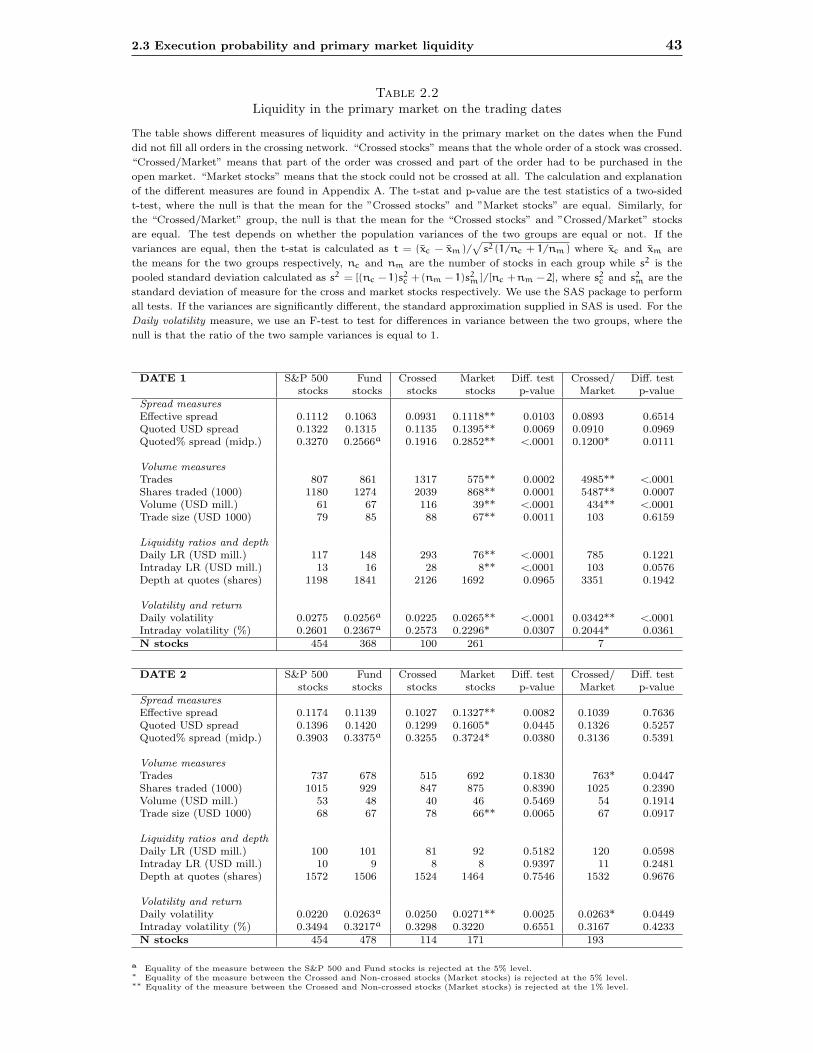
2.3 Execution probability and primary market liquidity 43
Table 2.2Liquidity in the primary market on the trading dates
The table shows different measures of liquidity and activity in the primary market on the dates when the Fund
did not fill all orders in the crossing network. “Crossed stocks” means that the whole order of a stock was crossed.
“Crossed/Market” means that part of the order was crossed and part of the order had to be purchased in the
open market. “Market stocks” means that the stock could not be crossed at all. The calculation and explanation
of the different measures are found in Appendix A. The t-stat and p-value are the test statistics of a two-sided
t-test, where the null is that the mean for the ”Crossed stocks” and ”Market stocks” are equal. Similarly, for
the “Crossed/Market” group, the null is that the mean for the “Crossed stocks” and ”Crossed/Market” stocks
are equal. The test depends on whether the population variances of the two groups are equal or not. If the
variances are equal, then the t-stat is calculated as t = (xc − xm)/√
s2(1/nc + 1/nm) where xc and xm are
the means for the two groups respectively, nc and nm are the number of stocks in each group while s2 is the
pooled standard deviation calculated as s2 = [(nc − 1)s2c + (nm − 1)s2
m]/[nc + nm − 2], where s2c and s2
m are the
standard deviation of measure for the cross and market stocks respectively. We use the SAS package to perform
all tests. If the variances are significantly different, the standard approximation supplied in SAS is used. For the
Daily volatility measure, we use an F-test to test for differences in variance between the two groups, where the
null is that the ratio of the two sample variances is equal to 1.
DATE 1 S&P 500 Fund Crossed Market Diff. test Crossed/ Diff. teststocks stocks stocks stocks p-value Market p-value
Spread measuresEffective spread 0.1112 0.1063 0.0931 0.1118** 0.0103 0.0893 0.6514Quoted USD spread 0.1322 0.1315 0.1135 0.1395** 0.0069 0.0910 0.0969Quoted% spread (midp.) 0.3270 0.2566a 0.1916 0.2852** <.0001 0.1200* 0.0111
Volume measuresTrades 807 861 1317 575** 0.0002 4985** <.0001Shares traded (1000) 1180 1274 2039 868** 0.0001 5487** 0.0007Volume (USD mill.) 61 67 116 39** <.0001 434** <.0001Trade size (USD 1000) 79 85 88 67** 0.0011 103 0.6159
Liquidity ratios and depthDaily LR (USD mill.) 117 148 293 76** <.0001 785 0.1221Intraday LR (USD mill.) 13 16 28 8** <.0001 103 0.0576Depth at quotes (shares) 1198 1841 2126 1692 0.0965 3351 0.1942
Volatility and returnDaily volatility 0.0275 0.0256a 0.0225 0.0265** <.0001 0.0342** <.0001Intraday volatility (%) 0.2601 0.2367a 0.2573 0.2296* 0.0307 0.2044* 0.0361N stocks 454 368 100 261 7
DATE 2 S&P 500 Fund Crossed Market Diff. test Crossed/ Diff. teststocks stocks stocks stocks p-value Market p-value
Spread measuresEffective spread 0.1174 0.1139 0.1027 0.1327** 0.0082 0.1039 0.7636Quoted USD spread 0.1396 0.1420 0.1299 0.1605* 0.0445 0.1326 0.5257Quoted% spread (midp.) 0.3903 0.3375a 0.3255 0.3724* 0.0380 0.3136 0.5391
Volume measuresTrades 737 678 515 692 0.1830 763* 0.0447Shares traded (1000) 1015 929 847 875 0.8390 1025 0.2390Volume (USD mill.) 53 48 40 46 0.5469 54 0.1914Trade size (USD 1000) 68 67 78 66** 0.0065 67 0.0917
Liquidity ratios and depthDaily LR (USD mill.) 100 101 81 92 0.5182 120 0.0598Intraday LR (USD mill.) 10 9 8 8 0.9397 11 0.2481Depth at quotes (shares) 1572 1506 1524 1464 0.7546 1532 0.9676
Volatility and returnDaily volatility 0.0220 0.0263a 0.0250 0.0271** 0.0025 0.0263* 0.0449Intraday volatility (%) 0.3494 0.3217a 0.3298 0.3220 0.6551 0.3167 0.4233N stocks 454 478 114 171 193
a Equality of the measure between the S&P 500 and Fund stocks is rejected at the 5% level.∗ Equality of the measure between the Crossed and Non-crossed stocks (Market stocks) is rejected at the 5% level.∗∗ Equality of the measure between the Crossed and Non-crossed stocks (Market stocks) is rejected at the 1% level.
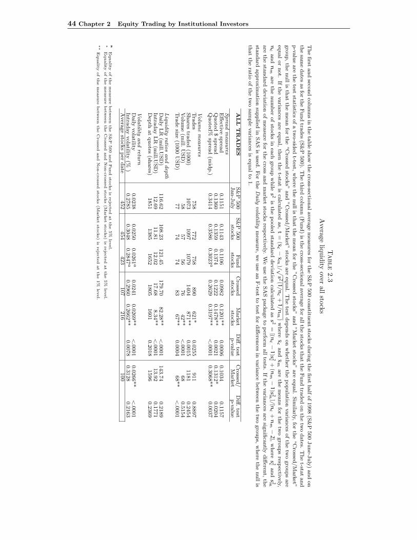
44 Chapter 2 Equity Trading by Institutional Investors
Table
2.3
Average
liquidityover
allstocks
The
first
and
second
colu
mns
inth
eta
ble
show
the
cross-sectio
nalavera
ge
mea
sures
for
the
S&
P500
constitu
ent
stock
sdurin
gth
efirst
half
of1998
(S&
P500
June-J
uly
)and
on
the
sam
edates
as
for
the
Fund
trades
(S&
P500).
The
third
colu
mn
(Fund)
isth
ecro
ss-sectionalavera
ge
for
all
the
stock
sth
at
the
Fund
traded
on
the
two
dates.
The
t-stat
and
p-v
alu
eare
the
teststa
tisticsofa
two-sid
edt-test,
where
the
null
isth
at
the
mea
nfo
rth
e”C
rossed
stock
s”and
”M
ark
etsto
cks”
are
equal.
Sim
ilarly,
for
the
“C
rossed
/M
ark
et”
gro
up,th
enull
isth
at
the
mea
nfo
rth
e“C
rossed
stock
s”and
”C
rossed
/M
ark
et”sto
cks
are
equal.
The
testdep
ends
on
wheth
erth
epopula
tion
varia
nces
ofth
etw
ogro
ups
are
equalor
not.
Ifth
evaria
nces
are
equal,
then
the
t-stat
isca
lcula
tedas,
t=
(xc
−x
m)/ √
s2(1
/n
c+
1/n
m)
where
xc
and
xm
are
the
mea
ns
for
the
two
gro
ups
respectiv
ely,
nc
and
nm
are
the
num
ber
ofsto
cks
inea
chgro
up
while
s2
isth
epooled
standard
dev
iatio
nca
lcula
tedas
s2
=[(n
c−
1)s
2c+
(nm
−1)s
2m]/
[nc
+n
m−
2],
where
s2c
and
s2m
are
the
standard
dev
iatio
nofm
easu
refo
rth
ecro
ssand
mark
etsto
cks
respectiv
ely.W
euse
the
SA
Spack
age
toperfo
rmall
tests.If
the
varia
nces
are
signifi
cantly
diff
erent,
the
standard
appro
xim
atio
nsu
pplied
inSA
Sis
used
.For
the
Daily
vola
tilitym
easu
re,w
euse
an
F-test
totest
for
diff
erences
invaria
nce
betw
eenth
etw
ogro
ups,
where
the
null
is
that
the
ratio
ofth
etw
osa
mple
varia
nces
iseq
ualto
1.
ALL
TR
AD
ES
S&
P500
S&
P500
Fund
Cro
ssedM
ark
etD
iff.test
Cro
ssed/
Diff
.test
Jan-J
uly
stock
ssto
cks
stock
ssto
cks
p-v
alu
eM
ark
etp-v
alu
eSprea
dm
easu
resE
ffectiv
esp
read
0.1
151
0.1
143
0.1
106
0.0
982
0.1
201**
0.0
006
0.1
034
0.1
157
Quoted
$sp
read
0.1
360
0.1
359
0.1
374
0.1
222
0.1
478**
0.0
021
0.1
312*
0.0
204
Quoted
%sp
read
(mid
p.)
0.3
414
0.3
586
0.3
023
a0.2
629
0.3
197**
<.0
001
0.3
068**
0.0
037
Volu
me
mea
sures
Tra
des
758
772
758
890
621*
0.0
255
911
0.8
897
Shares
traded
(1000)
1073
1097
1079
1404
871**
0.0
015
1181
0.2
454
Volu
me
(mill.
USD
)58
57
56
76
42**
<.0
001
68
0.5
154
Tra
de
size(1
000
USD
)77
74
74
83
67**
0.0
004
68**
<.0
001
Liqu
idity
ratio
sand
dep
thD
aily
LR
(mill.U
SD
)116.6
2108.2
3121.4
5179.7
082.2
8**
<.0
001
143.7
40.2
189
Intra
day
LR
(mill.U
SD
)12.6
911.8
112.0
217.6
88.3
4**
<.0
001
13.9
20.1
771
Dep
that
quotes
(shares)
1851
1385
1652
1805
1601
0.2
018
1596
0.2
369
Vola
tilityand
return
Daily
vola
tility0.0
238
0.0
250
0.0
261
a0.0
241
0.0
269**
<.0
001
0.0
266**
<.0
001
Intra
day
vola
tility(%
)0.2
785
0.3
048
0.2
847
a0.2
960
0.2
662**
0.0
078
0.3
128
0.2
163
Avera
ge
stock
sper
date
452
454
423
107
216
100
aEquality
ofth
em
easu
rebetw
een
the
S&
P500
and
Fund
stocks
isre
jecte
dat
the
5%
level.
∗Equality
ofth
em
easu
rebetw
een
the
Cro
ssed
and
Non-c
rosse
dsto
cks
(Mark
et
stocks)
isre
jecte
dat
the
5%
level.
∗∗
Equality
ofth
em
easu
rebetw
een
the
Cro
ssed
and
Non-c
rosse
dsto
cks
(Mark
et
stocks)
isre
jecte
dat
the
1%
level.
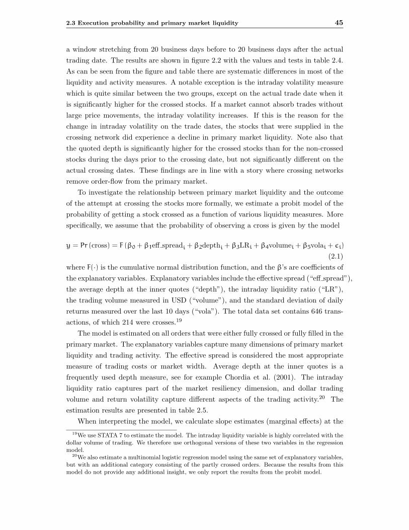
2.3 Execution probability and primary market liquidity 45
a window stretching from 20 business days before to 20 business days after the actualtrading date. The results are shown in figure 2.2 with the values and tests in table 2.4.As can be seen from the figure and table there are systematic differences in most of theliquidity and activity measures. A notable exception is the intraday volatility measurewhich is quite similar between the two groups, except on the actual trade date when itis significantly higher for the crossed stocks. If a market cannot absorb trades withoutlarge price movements, the intraday volatility increases. If this is the reason for thechange in intraday volatility on the trade dates, the stocks that were supplied in thecrossing network did experience a decline in primary market liquidity. Note also thatthe quoted depth is significantly higher for the crossed stocks than for the non-crossedstocks during the days prior to the crossing date, but not significantly different on theactual crossing dates. These findings are in line with a story where crossing networksremove order-flow from the primary market.
To investigate the relationship between primary market liquidity and the outcomeof the attempt at crossing the stocks more formally, we estimate a probit model of theprobability of getting a stock crossed as a function of various liquidity measures. Morespecifically, we assume that the probability of observing a cross is given by the model
y = Pr (cross) = F (β0 + β1eff spreadi + β2depthi + β3LRi + β4volumei + β5volai + εi)
(2.1)where F(·) is the cumulative normal distribution function, and the β’s are coefficients ofthe explanatory variables. Explanatory variables include the effective spread (“eff spread”),the average depth at the inner quotes (“depth”), the intraday liquidity ratio (“LR”),the trading volume measured in USD (“volume”), and the standard deviation of dailyreturns measured over the last 10 days (“vola”). The total data set contains 646 trans-actions, of which 214 were crosses.19
The model is estimated on all orders that were either fully crossed or fully filled in theprimary market. The explanatory variables capture many dimensions of primary marketliquidity and trading activity. The effective spread is considered the most appropriatemeasure of trading costs or market width. Average depth at the inner quotes is afrequently used depth measure, see for example Chordia et al. (2001). The intradayliquidity ratio captures part of the market resiliency dimension, and dollar tradingvolume and return volatility capture different aspects of the trading activity.20 Theestimation results are presented in table 2.5.
When interpreting the model, we calculate slope estimates (marginal effects) at the19We use STATA 7 to estimate the model. The intraday liquidity variable is highly correlated with the
dollar volume of trading. We therefore use orthogonal versions of these two variables in the regressionmodel.
20We also estimate a multinomial logistic regression model using the same set of explanatory variables,but with an additional category consisting of the partly crossed orders. Because the results from thismodel do not provide any additional insight, we only report the results from the probit model.
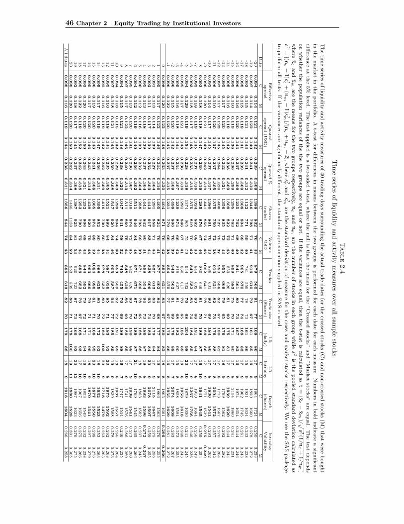
46 Chapter 2 Equity Trading by Institutional Investors
Table
2.4
Tim
eseries
ofliquidity
andactivity
measures
overall
sample
stocks
The
time
seriesofliq
uid
ityand
activ
itym
easu
resof40
tradin
gdays
surro
undin
gth
eactu
altra
de
dates
for
the
crossed
stock
s(C
)and
non-cro
ssedsto
cks
(M)
that
were
bought
inth
em
ark
etin
the
portfo
lio.
At-test
for
diff
erences
inm
eans
betw
eenth
etw
ogro
ups
isperfo
rmed
for
each
date
for
each
mea
sure.
Num
bers
inbold
indica
tea
signifi
cant
diff
erence
at
the
5%
level.
The
testapplied
isa
two-sid
edt-test,
where
the
null
isth
at
the
mea
nfo
rth
e”C
rossed
stock
s”and
”M
ark
etsto
cks”
are
equal.
The
testdep
ends
on
wheth
erth
epopula
tion
varia
nces
of
the
the
two
gro
ups
are
equal
or
not.
Ifth
evaria
nces
are
equal,
then
the
t-stat
isca
lcula
tedas
t=
(xc
−x
m)/ √
s2(1
/n
c+
1/n
m)
where
xc
and
xm
are
the
mea
ns
for
the
two
gro
ups
respectiv
ely,n
cand
nm
are
the
num
ber
of
stock
sin
each
gro
up
while
s2
isth
epooled
standard
dev
iatio
nca
lcula
tedas
s2
=[(n
c−
1)s
2c+
(nm
−1)s
2m]/
[nc
+n
m−
2],
where
s2c
and
s2m
are
the
standard
dev
iatio
nofm
easu
refo
rth
ecro
ssand
mark
etsto
cks
respectiv
ely.W
euse
the
SA
Spack
age
toperfo
rmall
tests.If
the
varia
nces
are
signifi
cantly
diff
erent,
the
standard
appro
xim
atio
nsu
pplied
inSA
Sis
used
.
Effectiv
eQ
uote
dQ
uote
d%
Share
sVolu
me
Tra
des
Tra
de
size
LR
LR
Depth
Intra
day
spre
ad
spre
ad
(USD
)sp
read
traded
USD
(Share
s)(d
aily
)In
traday
(share
s)Vola
tilityD
ate
CM
CM
CM
CM
CM
CM
CM
CM
CM
CM
CM
-20
0.0
94
0.1
14
0.1
21
0.1
42
0.2
39
0.3
09
1388
832
76
43
879
560
91
77
168
86
17
91864
1724
0.2
50
0.2
33
-19
0.0
97
0.1
14
0.1
22
0.1
40
0.2
41
0.3
10
1346
798
71
41
916
610
79
67
161
85
16
81820
1660
0.2
78
0.2
72
-18
0.0
93
0.1
15
0.1
21
0.1
43
0.2
41
0.3
12
1122
771
59
40
781
559
78
73
161
86
15
91931
1634
0.2
33
0.2
38
-17
0.0
95
0.1
15
0.1
19
0.1
41
0.2
39
0.3
09
1308
804
69
42
905
570
77
74
168
83
17
91962
1745
0.2
61
0.2
43
-16
0.0
96
0.1
16
0.1
20
0.1
43
0.2
37
0.3
09
1235
762
68
40
841
561
80
73
167
82
16
81974
1654
0.2
44
0.2
46
-15
0.0
95
0.1
10
0.1
19
0.1
36
0.2
36
0.2
99
1295
763
71
40
899
583
75
70
171
80
17
82154
1860
0.2
41
0.2
31
-14
0.0
95
0.1
16
0.1
19
0.1
42
0.2
38
0.3
09
1309
822
72
43
853
626
81
69
175
81
17
91939
1620
0.2
44
0.2
44
-13
0.0
95
0.1
17
0.1
20
0.1
45
0.2
42
0.3
21
1356
835
73
43
955
669
79
65
176
81
18
91799
1562
0.2
92
0.2
82
-12
0.0
97
0.1
17
0.1
23
0.1
45
0.2
44
0.3
20
1400
727
75
37
950
556
82
67
180
82
17
81773
1567
0.2
70
0.2
64
-11
0.0
96
0.1
10
0.1
20
0.1
37
0.2
37
0.3
05
1375
759
72
38
910
521
82
73
176
88
17
82094
1572
0.2
57
0.2
42
-10
0.0
93
0.1
14
0.1
17
0.1
45
0.2
37
0.3
17
1380
861
70
43
886
631
80
69
184
86
17
81836
1541
0.2
83
0.2
62
-90.0
96
0.1
20
0.1
21
0.1
49
0.2
42
0.3
19
1441
855
74
46
1002
641
78
71
189
86
17
91771
1539
0.2
75
0.2
49
-80.0
93
0.1
18
0.1
18
0.1
47
0.2
39
0.3
19
1285
876
67
46
880
649
81
70
188
87
16
10
1941
1545
0.2
59
0.2
54
-70.0
93
0.1
18
0.1
19
0.1
45
0.2
37
0.3
16
1324
862
68
43
844
632
83
68
191
84
17
81950
1684
0.2
56
0.2
49
-60.0
93
0.1
18
0.1
17
0.1
48
0.2
33
0.3
15
1375
819
70
42
849
582
83
74
184
85
17
92267
1756
0.2
46
0.2
36
-50.0
94
0.1
29
0.1
19
0.1
54
0.2
28
0.3
18
1374
965
75
50
944
732
76
68
204
98
20
10
1879
1636
0.2
41
0.2
45
-40.0
95
0.1
17
0.1
21
0.1
48
0.2
36
0.3
16
1291
846
67
41
860
617
76
65
185
89
16
81953
1618
0.2
48
0.2
43
-30.0
95
0.1
16
0.1
18
0.1
44
0.2
34
0.3
07
1239
874
66
42
819
627
81
68
182
90
15
81858
1594
0.2
72
0.2
55
-20.0
96
0.1
15
0.1
20
0.1
42
0.2
37
0.3
09
1499
806
76
39
948
562
81
69
176
88
17
72074
1668
0.2
83
0.2
67
-10.0
96
0.1
22
0.1
20
0.1
45
0.2
37
0.3
15
1231
779
66
38
854
570
77
67
173
86
16
81955
1629
0.2
81
0.2
72
00.0
98
0.1
20
0.1
22
0.1
48
0.2
63
0.3
20
1404
871
76
42
890
621
83
67
180
82
18
81805
1601
0.2
96
0.2
66
10.0
95
0.1
17
0.1
22
0.1
46
0.2
44
0.3
16
1405
824
76
41
877
602
84
68
177
84
19
81866
1563
0.2
76
0.2
55
20.0
91
0.1
13
0.1
14
0.1
39
0.2
27
0.3
04
1291
858
71
43
837
613
83
70
179
84
17
92115
1647
0.2
75
0.2
56
30.0
92
0.1
11
0.1
17
0.1
39
0.2
32
0.3
03
1443
917
83
44
828
606
93
74
183
84
20
92078
1597
0.2
59
0.2
55
40.0
95
0.1
13
0.1
18
0.1
39
0.2
37
0.3
04
1441
842
80
41
898
554
94
73
186
87
18
81983
1596
0.2
72
0.2
47
50.0
90
0.1
12
0.1
16
0.1
39
0.2
32
0.3
04
1258
795
69
39
871
596
78
65
188
88
18
81883
1582
0.2
37
0.2
45
60.0
94
0.1
12
0.1
19
0.1
40
0.2
36
0.3
02
1511
946
84
48
971
671
87
72
189
87
21
10
1799
1545
0.2
65
0.2
66
70.0
95
0.1
13
0.1
20
0.1
41
0.2
36
0.3
07
1310
874
72
45
842
626
83
70
190
88
17
91938
1541
0.2
73
0.2
60
80.0
97
0.1
17
0.1
22
0.1
46
0.2
40
0.3
13
1311
869
75
44
848
629
86
69
189
85
17
91741
1576
0.2
86
0.2
80
90.0
94
0.1
15
0.1
21
0.1
48
0.2
38
0.3
20
1047
641
58
32
745
455
76
69
188
88
16
71747
1514
0.2
46
0.2
35
10
0.0
94
0.1
18
0.1
15
0.1
42
0.2
29
0.3
03
1299
804
74
40
853
559
82
72
191
89
18
81987
1557
0.2
66
0.2
64
11
0.0
97
0.1
18
0.1
21
0.1
45
0.2
39
0.3
08
1547
920
84
46
905
587
94
77
185
89
19
91839
1588
0.2
78
0.2
73
12
0.0
95
0.1
16
0.1
18
0.1
44
0.2
35
0.3
05
1521
889
84
44
987
636
85
71
183
92
20
81975
1592
0.2
62
0.2
68
13
0.0
92
0.1
16
0.1
19
0.1
42
0.2
42
0.3
09
1416
730
80
38
978
532
80
72
182
103
20
91718
1479
0.2
53
0.2
63
14
0.0
95
0.1
17
0.1
19
0.1
47
0.2
36
0.3
11
1395
852
80
44
968
625
80
70
172
92
18
10
1932
1523
0.2
53
0.2
63
15
0.0
96
0.1
19
0.1
20
0.1
46
0.2
41
0.3
08
1665
974
89
49
1084
696
81
71
166
95
20
10
1877
1550
0.2
98
0.2
76
16
0.0
95
0.1
17
0.1
20
0.1
46
0.2
43
0.3
14
1429
920
79
48
963
666
79
71
171
96
18
91870
1541
0.2
97
0.2
79
17
0.0
93
0.1
20
0.1
20
0.1
50
0.2
43
0.3
21
1232
806
68
43
844
592
79
72
171
94
16
10
1853
1549
0.2
32
0.2
38
18
0.0
95
0.1
22
0.1
19
0.1
52
0.2
42
0.3
18
1252
790
72
44
896
652
76
67
168
93
17
10
1967
1656
0.2
75
0.2
66
19
0.0
92
0.1
18
0.1
17
0.1
45
0.2
37
0.3
08
1387
925
81
53
920
723
87
73
166
93
20
12
1987
1623
0.2
76
0.2
75
20
0.0
95
0.1
20
0.1
20
0.1
50
0.2
42
0.3
14
1466
1130
84
59
953
839
86
71
178
100
19
11
1880
1528
0.3
01
0.3
05
All
date
s0.0
95
0.1
16
0.1
19
0.1
44
0.2
38
0.3
11
1356
844
74
43
896
613
82
70
179
88
18
91918
1604
0.2
66
0.2
58

2.3 Execution probability and primary market liquidity 47
Figure 2.2 Time series average of liquidity and activity measuresThe figures show average time series plots of the different liquidity and activity measures. The actual trading
days are aligned at t=0. From the figures there seem to be a systematic difference in both liquidity and activity
over time between the group of stocks that were fully crossed and those that were not crossed at all. Similar
plots of the measures around the separate dates show the same systematic patterns.
0.00
0.02
0.04
0.06
0.08
0.10
0.12
0.14
-20 -10 0 10 20
Trading days
Eff
ectiv
e sp
read
Eff.spread Cross
Eff.spread Market
0.00
0.02
0.04
0.06
0.08
0.10
0.12
0.14
0.16
0.18
-20 -10 0 10 20
Trading days
Quo
ted
spre
adQouted $ spread Cross
Quoted $ spread Market
0.00
0.05
0.10
0.15
0.20
0.25
0.30
0.35
-20 -10 0 10 20
Trading days
Quo
ted
% s
prea
d
Quoted % spread Cross
Quoted % spread Market
0
200
400
600
800
1000
1200
1400
1600
1800
-20 -10 0 10 20
Trading days
Shar
es tr
aded
(10
00)
Shares traded Cross
Shares traded Market
0
10
20
30
40
50
60
70
80
90
100
-20 -10 0 10 20Trading days
Vol
ume
(USD
mill
)Vol USD Cross
Vol USD Market
0
500
1000
1500
2000
2500
3000
-20 -10 0 10 20
Trading days
Dep
th a
t quo
tes
(sha
res)
Depth at quotes Cross
Depth at quotes Market
0
50
100
150
200
250
-20 -10 0 10 20
Trading days
Dai
ly L
R (
mill
. USD
)
Daily LR Cross
Daily LR Market
0
5
10
15
20
25
-20 -10 0 10 20
Trading days
Intr
aday
LR
(m
ill U
SD)
Intraday LR Cross
Intraday LR Market
0.10
0.15
0.20
0.25
0.30
0.35
-20 -10 0 10 20
Trading days
Intr
aday
Vol
atili
ty
Intraday Volatility Cross
Intraday Volatility Market
0
200
400
600
800
1000
1200
1400
1600
-20 -10 0 10 20Trading days
Num
ber
of tr
ades
Trades Cross
Trades Market
30
40
50
60
70
80
90
100
-20 -10 0 10 20
Trading days
Ord
er s
ize
(100
0 U
SD)
Order size (1000 USD) Cross
Order size (1000 USD) Market
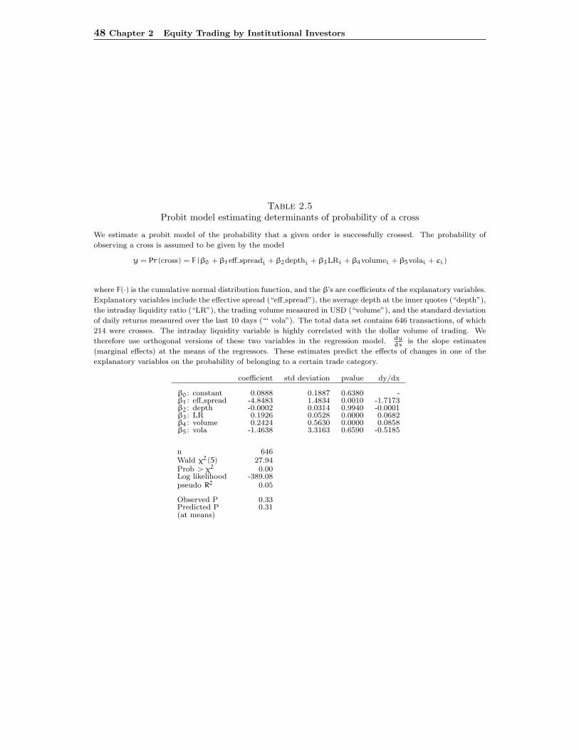
48 Chapter 2 Equity Trading by Institutional Investors
Table 2.5Probit model estimating determinants of probability of a cross
We estimate a probit model of the probability that a given order is successfully crossed. The probability of
observing a cross is assumed to be given by the model
y = Pr (cross) = F (β0 + β1eff spreadi + β2depthi + β3LRi + β4volumei + β5volai + εi)
where F(·) is the cumulative normal distribution function, and the β’s are coefficients of the explanatory variables.
Explanatory variables include the effective spread (“eff spread”), the average depth at the inner quotes (“depth”),
the intraday liquidity ratio (“LR”), the trading volume measured in USD (“volume”), and the standard deviation
of daily returns measured over the last 10 days (“‘ vola”). The total data set contains 646 transactions, of which
214 were crosses. The intraday liquidity variable is highly correlated with the dollar volume of trading. We
therefore use orthogonal versions of these two variables in the regression model. dydx
is the slope estimates
(marginal effects) at the means of the regressors. These estimates predict the effects of changes in one of the
explanatory variables on the probability of belonging to a certain trade category.
coefficient std deviation pvalue dy/dx
β0: constant 0.0888 0.1887 0.6380 -β1: eff spread -4.8483 1.4834 0.0010 -1.7173β2: depth -0.0002 0.0314 0.9940 -0.0001β3: LR 0.1926 0.0528 0.0000 0.0682β4: volume 0.2424 0.5630 0.0000 0.0858β5: vola -1.4638 3.3163 0.6590 -0.5185
n 646Wald χ2(5) 27.94Prob > χ2 0.00Log likelihood -389.08pseudo R2 0.05
Observed P 0.33Predicted P 0.31(at means)

2.4 Limit order simulation 49
means of the regressors (dydx in table 2.5).21 These estimates predict the effects of changes
in one of the explanatory variables on the probability of belonging to a certain tradecategory. Note also that our estimation is simplified by the fact that our data onlycontains buy orders; we need not adjust for the direction of trade.
The estimated probit model in table 2.5 confirms the result in 2.3 that the probabilityof finding a counterparty in the crossing network is positively related to the liquidityof the stock in the primary market. The probability of a cross is higher the lower theeffective spread, the higher the intraday liquidity ratio, and the higher the dollar tradingvolume in the primary market. This implies that stocks that are easy to cross are alsohighly traded in the market and have low costs measured by the effective spread.22
To sum up, our results indicate that the most liquid and actively traded stocks in theprimary market also have the highest probability of being crossed. Our results indicatethat both liquidity differences and private information may explain the difference in expost abnormal return between the crossed and non-crossed stocks found in Næs andØdegaard (2000). A significant difference in liquidity between the two groups of stocks,also on other dates than the trading dates, may indicate that investors need a higherreturn to hold the non-crossed stocks. On the other hand, it is hard to believe thatliquidity differences between the 500 largest and most liquid companies in the US canexplain a difference in abnormal performance between the two group of stocks of 1percent over 20 days as found in Næs and Ødegaard (2000).
2.4 Limit order simulation
To judge whether trading in the primary market is more expensive than crossing, weneed additional information on the costs of obtaining the stocks directly in the market.Since the Fund was trading in the 500 largest and most liquid companies in the USmarket, it could well be that a strategy of buying them directly in the market wouldhave been less expensive than the crossing strategy followed by the Fund.
In this section, we examine the cost of the opportunistic crossing strategy relativeto alternative submission strategies. In addition to a cost comparison, the simulationsallow us to obtain a measure of immediacy. This is an important dimension of liquiditywhich is crucial for transaction costs, and which is not directly captured by the measuresused in the previous section.
21For non-linear probability models such as the probit and the logit model, we have that the effectsof changes in one of the explanatory variables will vary with the value of the regressors.
22Market depth and return volatility do not have significant effects on the probability of getting astock in the crossing network.

50 Chapter 2 Equity Trading by Institutional Investors
2.4.1 Literature
Crossing networks There are two theoretical papers on crossing networks; Hender-shott and Mendelson (2000) and Donges and Heinemann (2001). There is also closelyrelated literature on the ability of multiple competing trading venues to coexist, see forexample Chowdhry and Nanda (1991), Easley et al. (1996a) and Seppi (1990).23
Hendershott and Mendelson (2000) develop a complex model where different typesof heterogenous liquidity traders and informed traders choose between a competitivedealer market and a crossing network. There are two types of informed traders: onetype with short-lived information and one type with long-lived information. Short-livedinformation cannot be exploited in the crossing network, but traders with long-livedinformation can first try trading in the crossing network and then go to the dealermarket if they are not able to cross. Trader strategies are modeled as Nash strategies:each trader chooses his or her best response given her expectation of all other traders’strategies.24 The model solution consists of multiple equilibria. All equilibria are char-acterized by three cutoff values that segment liquidity traders into the following four(some possible empty) sets of strategies:
• do not trade,
• trade exclusively on the crossing network,
• trade opportunistically in the crossing network, i.e. attempt to trade in the cross-ing network, and then go to the dealer market if you cannot get an execution inthe crossing network, and
• trade only in the dealer market.
The implications on dealers’ spread from the introduction of a crossing network areshown to depend on the types of traders in the market. With no informed trading,the negative “cream-skimming” effect dominates the positive effect of attracting neworder flow. This is because the crossing network has a negative impact on the dealers’inventory and fixed costs, and because orders going first to the crossing network imposehigher costs on the dealer market than those going directly to the dealer market.25 Withshort-lived information, the low order-submission costs ensure that the introduction ofa crossing network will always raise the dealers’ spread. This is because the crossingnetwork reduces the order flow from liquidity traders without affecting the order flow
23There is an extensive literature on related subjects such as (i) the costs of using electronic com-munication networks (ECNs) (see Barclay et al. (2001), Barclay and Hendershott (2002), Coppejeansand Domowitz (1999), Domowitz and Steil (1998)), and Hasbrouck and Saar (2001) and (ii) why sometraders may want to trade outside the primary market (see Easley et al. (1996a) and Seppi (1990)).
24Trading decisions are based on the trader’s reservation value, the spread cost, a crossing commission,the probability of getting a cross executed, and an impatience factor.
25Order flow sent to the crossing network leaves the dealers with fewer orders to cover the inventoryand fixed costs, leading to higher average costs per order.
2.4 Limit order simulation 51
from informed traders. Under most circumstances, the crossing network will also in-crease dealer spreads when information is long-lived. However, this can be offset if thecrossing network manages to attract sufficient new liquidity traders.
The Donges and Heinemann (2001) model is considerably simpler than the Hen-dershott and Mendelson (2000) model. Competition for order flow is modeled as acoordination game. The central variable is the value of trading, or, equivalently, thedisutility from non-executed orders in the crossing network. Three different settings areanalyzed. In the first setting all traders face an identical and certain cost of not gettingan order executed in the crossing network. In this case, there are multiple equilibriaas in the Hendershott and Mendelson model. In the second setting, all traders face anidentical, but unknown cost of non-execution. By introducing private signals on thevalue of this cost, a unique equilibrium with market consolidation is shown to exist. Ac-cording to Dønges and Heinemann, assets with low price volatility and large turnoverswill be traded at a crossing network, while assets with high volatility or small volumeswill be traded at dealer markets. In the third setting, the cost of non-execution is nolonger assumed to be common among the traders. In this case, and provided that thedisutility from non-execution differs sufficiently, there exists a unique equilibrium withmarket fragmentation. The two models provide few unambiguous implications. Rather,they form a framework for discussing important questions.
Limit order simulations The probability of non-execution is a central variable forboth limit orders and orders submitted to a crossing network, especially for investors whoare precommited to trade. Much cited papers on the modeling of execution probabilityand execution time of limit orders are Angel (1994), Lo et al. (2002), and Hollifield et al.(1999).26 Angel (1994) derives closed form solutions for the probability of limit orderexecution when orders arrive according to a Poisson process and prices are discrete.Lo et al. (2002) develop an econometric model of limit order execution times usingsurvival analysis and estimate it using actual limit order data. Hollifield et al. (1999)also develop, estimate, and test an econometric model of a pure limit order market.Their model describes the tradeoff between the limit order price and the probability ofexecution.
There are also several interesting empirical papers on the use of limit orders. Choand Nelling (2000) investigate the probability of limit order executions for a selection ofstocks at the NYSE. They find that the probability of execution is higher for sell ordersthan for buy orders, lower when the limit price is farther away from the prevailingquote, lower for larger trades, higher when spreads are wide and higher in periods of
26There is also an extensive theoretical literature on the effect of limit orders on the price discoveryprocess as well as the relative profitability of limit orders compared to market orders. Important contri-butions include Foucault (1999), Glosten (1994), Easley and O’Hara (1992), Parlour (1996), Chakrevartyand Holden (1995), Seppi (1997).

52 Chapter 2 Equity Trading by Institutional Investors
higher volatility. In addition, they find that the longer a limit order is outstanding,the less likely it is to execute, and that limit orders tends to be submitted at the bid-ask midpoint. Examining order flow and limit order submission strategies in a purelimit order market (the Paris Bourse), Biais et al. (1995) find that traders’ limit orderstrategies depend on the market conditions: traders submit more market orders whenspreads are narrow and submit more limit orders when spreads are wide, as shown byAngel (1994). Harris and Hasbrouck (1996) compare the performance of limit ordersrelative to market orders using the TORQ database. They find that limit orders placedat the quotes or further into the market outperform market orders when the spread islarger than the tick size. They therefore argue that limit orders in some cases can reduceexecution costs compared to market orders. Handa and Schwartz (1996) approach theproblem from a different angle by examining the performance of limit orders versusmarket orders by “submitting” hypothetical limit orders on the actual price paths of thethirty Dow Jones Industrial firms traded on the NYSE. Since they are using simulations,they can also evaluate the cost of non-executed limit orders. Their main finding is thatnon-execution costs are positive, but not always significant.
2.4.2 Simulation design
We base our simulations on the strategies followed by the liquidity traders in the Hender-shott and Mendelson (2000) model, ignoring the ”no trade” category. The first strategy,opportunistic crossing, is the actual strategy followed by the Fund. The second strategy,pure cross, is the case where the trader only submit orders to the crossing network. Inthis case, the trader has a low demand for immediacy/liquidity.
The third strategy is the case where the orders are only submitted to the market.Orders submitted to the market can be market orders or limit orders. An uninformedinvestor such as the Fund would generally prefer the lower costs and lower executionprobability associated with limit orders to the immediacy provided by market orders. Onthe other hand, orders that are worked into the market may help reducing transactionscosts. Domowitz (2001) shows that when the trader is ”monitoring the book”, andthus strategically searching for liquidity and favorable execution possibilities, a marketorder strategy (working the order) may reduce transaction costs considerably and reducethe price impact cost for large orders. Angel (1997) shows that about 30 percent of themarket orders submitted through the SuperDot system experienced a price improvementof about USD 0.04 per share.
The best way to simulate a market order strategy would probably be to set up andestimate a dynamic model that minimizes transaction costs given the stock and marketcharacteristics at the time of submission, such as the order flow, the depth of the limitorder book, the volatility etc. The realism of such an ex post optimized strategy wouldbe very hard to judge, however. Moreover, an “in sample” optimized strategy based on
2.4 Limit order simulation 53
data from a limited period of time have restricted interest “out of sample”. Due to theobvious difficulties in constructing a market order simulation taking into account theplethora of strategic decisions involved, we restrict our analysis to simulating differentlimit order strategies. In this way, we get an interesting additional liquidity statisticand a realistic “lower bound” on the implicit execution costs of alternative submissionstrategies in the primary market.27
The closest proxy to a market order strategy in our simulations is a marketable limitorder strategy (MLO). A MLO strategy is a limit order strategy that is more aggressive(”in to the market”) than an ”at the quote” (ATQ) limit order strategy. The maindifference between an ATQ and MLO strategy is that the limit price is set at the bidand ask prices respectively. The higher limit price of the MLO strategy increases theexecution probability and speed relative to an ATQ strategy. However, this increasedimmediacy may come at a cost.28
Note that both limit orders and crossing orders have a potentially costly adverseselection component. From the buyer’s perspective, a limit order is filled when there isadverse price movement and not filled when the stock value increases. Both cases mayor may not be due to new information. Similarly, the probability of being a successfulbuyer in a crossing network increases with the number of investors on the selling sideof the market. As for limit orders, if there are informed investors (with long-livedinformation) in the crossing network, the execution probability of a buy order decreasesif the information is positive.29
Limit order simulations All limit order submissions are simulated using the samestocks and dates that applied when the Fund first tried to cross the orders. The firstlimit order simulation (LO1) is identical to the simple simulation strategy in Handa andSchwartz (1996), i.e. we do not take into account the actual order sizes traded by theFund. In other words, we assume that only one share is traded in each stock. At thebeginning of each crossing date, a limit order is submitted with a limit price equal tothe opening bid-quote (”at the quote” limit order strategy) for each stock that the Fundtried to cross. If a trade with a price lower than the limit order price is observed duringthe day, the order is assumed to be filled. If an order is not filled, we assume that itis executed at the opening price the next day. Thus, we implicitly assume an investor
27As noted by Lo et al. (2002), there will be a general bias in favor of early execution of simulatedlimit orders compared to actual limit orders. Moreover, the simulation does not track where in thelimit order queue our order is at any point in time, only the price priority. This probably affects the fillrate and execution time of the orders in favor of the simulated orders compared to actual limit orderexecution.
28The cost differential between the two types of strategies may vary over time depending on marketconditions. The execution probability of a marketable limit order is likely to be lower in a bear marketrelative to a bull market.
29Næs and Ødegaard (2000) find evidence that the Fund was “crowded out” by informed investors onthe same side of the market.

54 Chapter 2 Equity Trading by Institutional Investors
who is pre-committed to trade the stocks. During the transition period, the Fund wastracking an index with a limit on the relative volatility between the transition portfolioand the benchmark. Thus, even though the trades probably could have been workedmore carefully into the market the next day, the penalty for unexecuted orders whichfollow from our assumptions is not completely unrealistic. Because we are ignoring ordersize, the first limit order simulation constitutes a lower bound on transaction costs.
In the second simulation (LO2), we split the actual order size into suborders. Thenumber and size of the suborders are determined by the average order size traded in thestock at t−1. In addition, we have one residual suborder of a smaller size (if necessary).All the suborders are assumed to be submitted sequentially. Thus, at the beginning ofthe trading day, the first suborder is submitted as an ”at the quote” limit order. Asuborder is assumed filled if the observed execution price is less than the limit-pricewithout taking into account the size of the suborder. When a suborder is filled, thenext suborder is submitted at the bid quote following the fill (”chasing the market”).Unfilled orders are assumed to be executed at the opening price the next day.30
The third limit order simulation (LO3) is the most realistic because here we alsotake into account the size of the suborders. The strategy is similar to LO2 exceptthat we also examine whether the size of the suborder is less than or equal to the sizeof the actual order executed in the market. A suborder is only assumed filled if theobserved execution price is less than the limit price and the size is equal to or largerthan the size of our order. Due to price priority, our hypothetical order would undermost circumstances execute before the observed trade since our order would be the lastin the queue at our limit price.
A problem with this type of simulation is that the hypothetical orders most likelywould have changed the structure of the market in the stocks if they had actuallybeen submitted. Furthermore, Lo et al. (2002) note than the results from simulationswith actual limit-order data underestimate the execution times in a real world tradingsituation. The execution time for a real limit order is a function of the order size,the limit price and the current market conditions, and a trader would generally varythe order submission strategy based on current and expected market conditions. Suchfactors are obviously very hard to capture in a simulation approach like ours. On theother hand, we do know the order sizes of the actual strategy and we do take these intoaccount in the LO2 and LO3 simulations, which probably reduces the bias.
Pure crossing simulation A pure crossing strategy is defined as a strategy where thetrader only trades in the crossing network. According to Hendershott and Mendelson(2000), the low liquidity preference traders who would follow this type of strategy aremost likely to benefit from the existence of a crossing network. To simulate this strategy
30The unexecuted orders are assumed submitted to the pre-trade auction without affecting the openingprice.
2.4 Limit order simulation 55
we use the actual price data for the stocks that the Fund was able to cross. For thestocks that the Fund was not able to cross, we assume crossing over the next 10 days.Hence, the opportunity costs are simulated, but the identity of stocks that could not becrossed are not. The choice of a 10-day trading window for calculating the opportunitycosts is based on the statistics on order fills in Conrad et al. (2001b): the 95th percentconfidence interval for getting an order filled in an external crossing system is reportedto be 10 days. Thus, on each crossing date we take the stocks that did not cross andassume that they were crossed over the next 10-day period to the equally weighted closeprice over the 10-day period.
2.4.3 Measuring trading costs
In order to compare the performance of different submission strategies we must apply ameasure of transaction costs. Current empirical academic literature on transaction costsare to a large degree based on versions of a theoretical measure which was first proposedby Treynor (1981) and which Perold (1988) later called the implementation shortfall.The implementation shortfall is defined as the difference in performance between theportfolio of actual trades and a matching paper portfolio in which the stock returns arecomputed assuming that the trades were executed at the prices prevailing on the dateof the decision to trade. In this way, both explicit cost components such as brokers fees,and implicit components such as spread costs, price impact costs, and costs related todelayed or uncompleted trading (opportunity costs) are captured. The approach alsoovercomes the problem of measuring costs on an individual trade basis when the orderconsists of a package of sub-trades 31. Keim and Madhavan (1998) and Conrad et al.(2001b) suggest an empirical version of the implementation shortfall approach:
total cost = explicit cost + implicit cost
={
commission per sharePd
}+
{[αPa
Pd+ (1 − α)Pd+x
Pd] − 1
} (2.2)
where Pd is the closing price for the stock on the day before the decision to trade, Pa
is the average price for all the executed trades in the order, α is the fill rate, and Pd+x
is the closing price x number of days after the decision date, i.e. the unfilled portion ofan order is assumed settled x days after the decision date.
We use the same measure as in Conrad et al. (2001b), except that we assume thatthe non-crossed orders in the pure crossing strategy are settled at the average of theclosing prices over the x days after the decision date. In addition, since we cannot easilyget good estimates for the explicit costs related to the trades that we simulate, the cost
31Much of the relevant research on the measurement of transaction costs is summarized in Keim andMadhavan (1998)

56 Chapter 2 Equity Trading by Institutional Investors
comparison is made on the basis of implicit costs only. Thus, our cost comparison is notbased on total execution costs. A more serious problem is related to the limited numberof trading days in our data set. The implicit cost estimate is intended to account forthe price impact of orders. However, the price difference between Pa and Pd will also beaffected by general market movements between the two observation times. Essentially,the measure assumes that the main source of price impact is our order. When we lookat averages for trades on many different dates, this is not a big problem, because themarket movement will tend to wash out in the average32. However, if we look at tradesconcentrated on a few dates, the general market movements at these dates will affectthe measured costs. As we shall see, this is a particular problem for the market ordersin our data set because they are concentrated on only three days.
Empirical studies document that the magnitude of different cost components varywith factors such as order size, intraday timing of the trade, stock liquidity, marketdesign and investment style. Hence, to measure costs properly, detailed data on theentire order submission process is required. For the actual submission strategy followedby the Fund, we have access to such data. For the simulated strategies, however, theresults will necessarily be driven to some extent by our own assumptions.
2.4.4 Results
For the orders that were executed on the day following the initial attempt at internalcrossing, the total cost should be decomposed into one component associated with thedelay of the order in the internal crossing network, and one component associated withthe final execution in an external crossing network or in the primary market. Table 2.6decompose the implicit costs for the Fund’s order submission strategy into these twocomponents.
Including the delay costs, the average implicit cost for all crossed orders was 0.11percent, and the average implicit cost for all market orders was -0.74 percent. Thisimplies an average implicit cost for all orders of -0.03. Some care should be takenwhen interpreting the negative implicit costs for the market orders. Because the orderspurchased in the primary market are concentrated on three trading days only, the costestimates are quite sensitive to the market movements on these days. Ignoring the delaycomponent, the average implicit cost for all market orders was about 0.25 percent. TheFund incurred delay costs for market orders on one occasion. The market went markedlydown on this day, leaving the Fund with an implicit delay cost for the non-crossed ordersof -1.79 percent. Because the non-crossed orders had to be bought in the market on thefollowing day, an average additional cost of 0.48 percent was incurred, giving a totalimplementation shortfall cost of -1.31 percent.
32Keim and Madhavan (1997) show that the average daily return on stocks is small compared to theprice impact from a trade.
2.4 Limit order simulation 57
Measured over some time, the daily market movements are small compared to theprice impact costs, as shown in Keim and Madhavan (1997). Hence, for large samples,adjusting for daily market returns does not make much difference. However, in ourcase, the cost measure is likely to be largely driven by the market movement. Keim andMadhavan (1997) argue that one should not try to adjust for market movements becausethey are a part of the timing cost for the order submission strategy. If so, the averageimplicit cost associated with the delay of orders in the private internal crossing networkof -0.121 percent should be interpreted as a negative timing cost. On the other hand,the fact that the drop in market values on one of the trading days was large enough tohave a significant effect on the total implementation shortfall cost of the actual strategy,suggests that the true costs of opportunistic crossing may be underestimated.
What the discussion above highlights most of all is that cost measures based onthe implementation shortfall over a few days should be interpreted with great caution.Due to the non-synchronous nature of the Fund’s market trades relative to the close-to-close returns on the SP 500 index, a correct adjustment for the market movementwould involve the actual timing of the trades during the day as well as the intradaySP 500 returns. None of which are easily obtainable. What we want is to set up ahorse race between the opportunistic crossing strategy and certain alternative ordersubmission strategies. If the alternative strategies cannot beat the strategy when thenegative delay costs are excluded, they surely cannot beat the strategy when these costsare included. In Table 2.7, we have therefore compared the estimated execution costsfor the simulated strategies with the actual average execution costs excluding the delaycosts.33 That is, all cost estimates in the table are in percent of the closing price on theday before the trade.34
Examining the execution costs for the simulated strategies in table 2.7, we findthat neither the pure crossing strategy nor the two first limit order strategies (LO1and LO2) have significantly different execution costs from the opportunistic crossingstrategy. Thus, not even the most simplistic and unrealistic limit order simulation(LO1), which constitute our ”lower bound” on primary market execution costs, is ableto significantly beat the opportunistic crossing strategy. The most realistic limit orderstrategy (LO3) is significantly more expensive than the opportunistic crossing strategy,with costs of about 0.24 percent. In addition, we have not taken into account that theexplicit costs in crossing networks are lower than in the primary market. Hence, thetotal execution costs would overwhelmingly favor the opportunistic crossing strategy, orpotentially the pure crossing strategy.
33What we ignore, however, is that the high volatility in the market at this particular day may haveaffected the outcome with respect to what stocks we were able to achieve in the crossing networks, assuggested in Domowitz (2001).
34Næs and Ødegaard (2000) also estimate the explicit costs for the Fund’s strategy. The equallyweighted average explicit costs for all orders were 3 percent. For the crossed orders and the non-crossedorders, the explicit costs were 3 percent and 5 percent respectively.
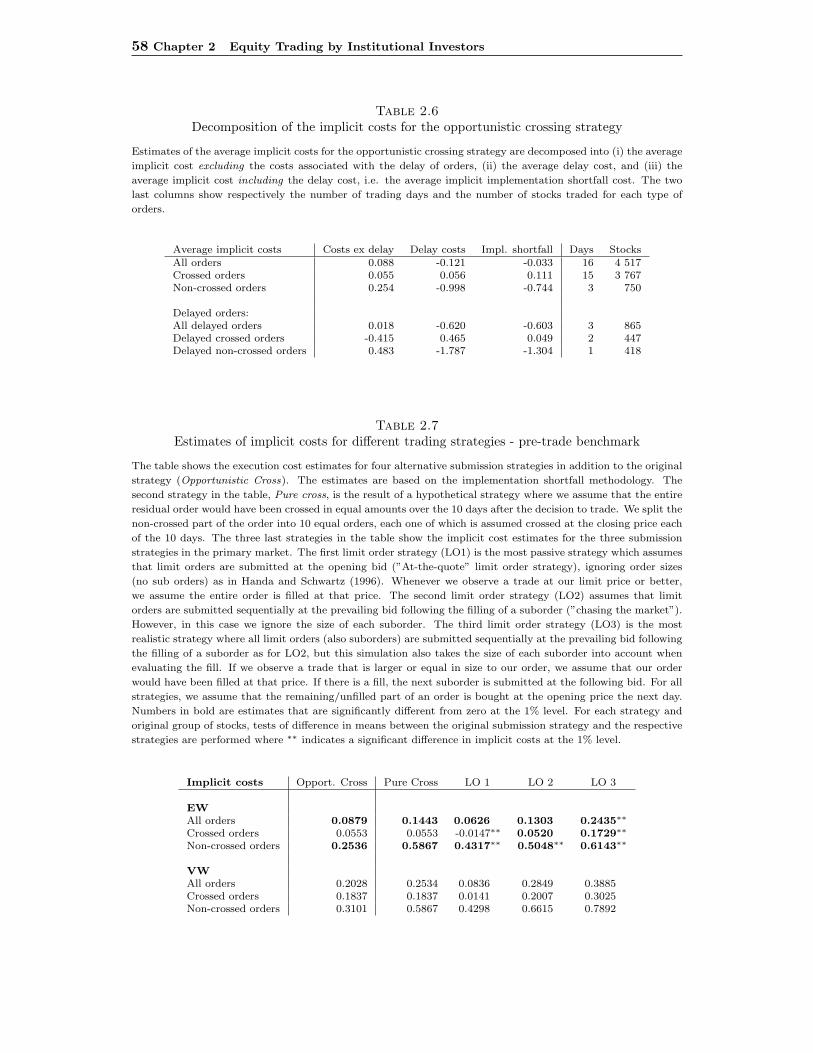
58 Chapter 2 Equity Trading by Institutional Investors
Table 2.6Decomposition of the implicit costs for the opportunistic crossing strategy
Estimates of the average implicit costs for the opportunistic crossing strategy are decomposed into (i) the average
implicit cost excluding the costs associated with the delay of orders, (ii) the average delay cost, and (iii) the
average implicit cost including the delay cost, i.e. the average implicit implementation shortfall cost. The two
last columns show respectively the number of trading days and the number of stocks traded for each type of
orders.
Average implicit costs Costs ex delay Delay costs Impl. shortfall Days StocksAll orders 0.088 -0.121 -0.033 16 4 517Crossed orders 0.055 0.056 0.111 15 3 767Non-crossed orders 0.254 -0.998 -0.744 3 750
Delayed orders:All delayed orders 0.018 -0.620 -0.603 3 865Delayed crossed orders -0.415 0.465 0.049 2 447Delayed non-crossed orders 0.483 -1.787 -1.304 1 418
Table 2.7Estimates of implicit costs for different trading strategies - pre-trade benchmark
The table shows the execution cost estimates for four alternative submission strategies in addition to the original
strategy (Opportunistic Cross). The estimates are based on the implementation shortfall methodology. The
second strategy in the table, Pure cross, is the result of a hypothetical strategy where we assume that the entire
residual order would have been crossed in equal amounts over the 10 days after the decision to trade. We split the
non-crossed part of the order into 10 equal orders, each one of which is assumed crossed at the closing price each
of the 10 days. The three last strategies in the table show the implicit cost estimates for the three submission
strategies in the primary market. The first limit order strategy (LO1) is the most passive strategy which assumes
that limit orders are submitted at the opening bid (”At-the-quote” limit order strategy), ignoring order sizes
(no sub orders) as in Handa and Schwartz (1996). Whenever we observe a trade at our limit price or better,
we assume the entire order is filled at that price. The second limit order strategy (LO2) assumes that limit
orders are submitted sequentially at the prevailing bid following the filling of a suborder (”chasing the market”).
However, in this case we ignore the size of each suborder. The third limit order strategy (LO3) is the most
realistic strategy where all limit orders (also suborders) are submitted sequentially at the prevailing bid following
the filling of a suborder as for LO2, but this simulation also takes the size of each suborder into account when
evaluating the fill. If we observe a trade that is larger or equal in size to our order, we assume that our order
would have been filled at that price. If there is a fill, the next suborder is submitted at the following bid. For all
strategies, we assume that the remaining/unfilled part of an order is bought at the opening price the next day.
Numbers in bold are estimates that are significantly different from zero at the 1% level. For each strategy and
original group of stocks, tests of difference in means between the original submission strategy and the respective
strategies are performed where ∗∗ indicates a significant difference in implicit costs at the 1% level.
Implicit costs Opport. Cross Pure Cross LO 1 LO 2 LO 3
EWAll orders 0.0879 0.1443 0.0626 0.1303 0.2435∗∗
Crossed orders 0.0553 0.0553 -0.0147∗∗ 0.0520 0.1729∗∗
Non-crossed orders 0.2536 0.5867 0.4317∗∗ 0.5048∗∗ 0.6143∗∗
VWAll orders 0.2028 0.2534 0.0836 0.2849 0.3885Crossed orders 0.1837 0.1837 0.0141 0.2007 0.3025Non-crossed orders 0.3101 0.5867 0.4298 0.6615 0.7892
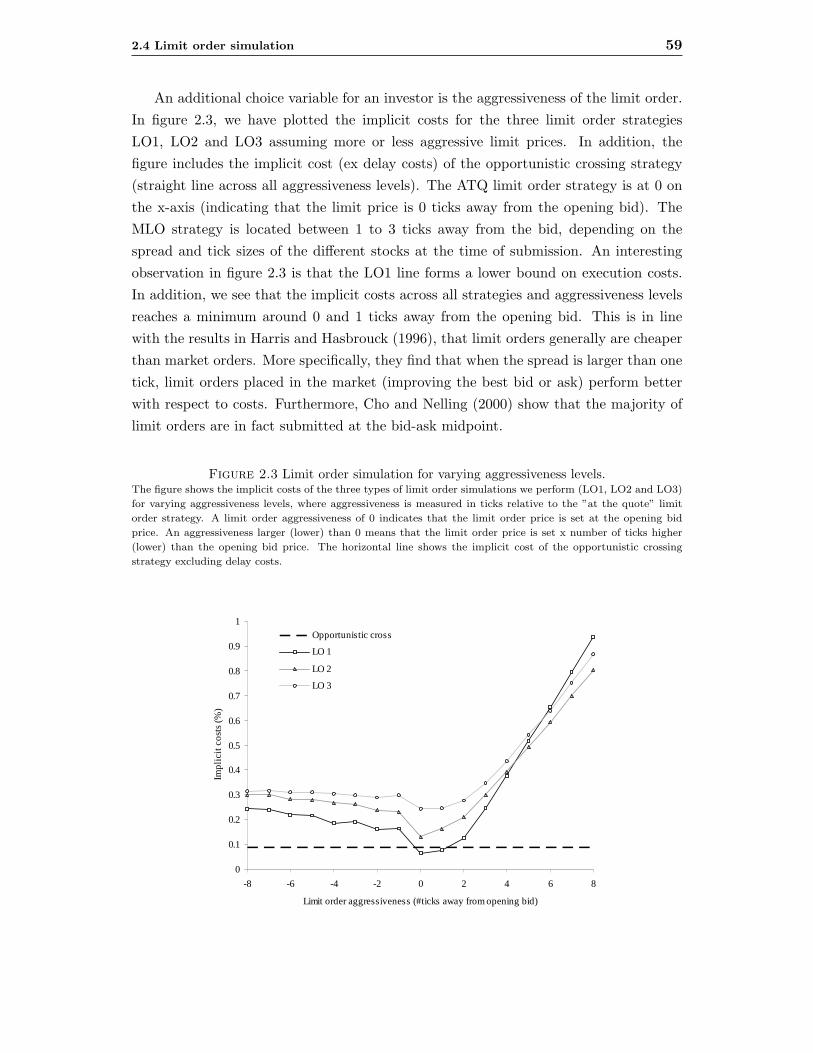
2.4 Limit order simulation 59
An additional choice variable for an investor is the aggressiveness of the limit order.In figure 2.3, we have plotted the implicit costs for the three limit order strategiesLO1, LO2 and LO3 assuming more or less aggressive limit prices. In addition, thefigure includes the implicit cost (ex delay costs) of the opportunistic crossing strategy(straight line across all aggressiveness levels). The ATQ limit order strategy is at 0 onthe x-axis (indicating that the limit price is 0 ticks away from the opening bid). TheMLO strategy is located between 1 to 3 ticks away from the bid, depending on thespread and tick sizes of the different stocks at the time of submission. An interestingobservation in figure 2.3 is that the LO1 line forms a lower bound on execution costs.In addition, we see that the implicit costs across all strategies and aggressiveness levelsreaches a minimum around 0 and 1 ticks away from the opening bid. This is in linewith the results in Harris and Hasbrouck (1996), that limit orders generally are cheaperthan market orders. More specifically, they find that when the spread is larger than onetick, limit orders placed in the market (improving the best bid or ask) perform betterwith respect to costs. Furthermore, Cho and Nelling (2000) show that the majority oflimit orders are in fact submitted at the bid-ask midpoint.
Figure 2.3 Limit order simulation for varying aggressiveness levels.The figure shows the implicit costs of the three types of limit order simulations we perform (LO1, LO2 and LO3)
for varying aggressiveness levels, where aggressiveness is measured in ticks relative to the ”at the quote” limit
order strategy. A limit order aggressiveness of 0 indicates that the limit order price is set at the opening bid
price. An aggressiveness larger (lower) than 0 means that the limit order price is set x number of ticks higher
(lower) than the opening bid price. The horizontal line shows the implicit cost of the opportunistic crossing
strategy excluding delay costs.
0
0.1
0.2
0.3
0.4
0.5
0.6
0.7
0.8
0.9
1
-8 -6 -4 -2 0 2 4 6 8
Limit order aggressiveness (#ticks away from opening bid)
Impl
icit
cost
s(%
)
Opportunistic cross
LO 1
LO 2
LO 3
60 Chapter 2 Equity Trading by Institutional Investors
By looking more carefully at the crossed/non-crossed groups, we find that the non-crossed stocks have the highest execution costs regardless of submission strategy. Inthe previous section, we found that stocks that are not supplied in the crossing networkare less liquid than stocks that are easily crossed. The higher execution costs for thesestocks support this finding: these stocks are also the most difficult to fill in the primarymarket. Note also that the opportunity costs constitute a large part of the executioncosts for orders in these less liquid stocks. Since unfilled limit orders generally are forstocks that rise in value, these orders are penalized by the execution at the openingprice the next day. This result, together with the high costs found for the pure crossingstrategy, supports the finding in Næs and Ødegaard (2000) that the stocks bought inthe market had a high ex post return.
Overall, our results strongly favor the opportunistic crossing strategy as a cost-effective submission strategy, especially when the difference in explicit costs betweenthe crossing network and primary market is taken into account. Furthermore, it isimportant to recognize that the orders examined here are for the most liquid and largestcompanies in the US. Thus, even the stocks with the potentially lowest execution costsin the primary market would have been cheaper to obtain in the crossing network.
In table 2.8, we have calculated the fill rates for all orders in panel (a), and thefill rates across groups of orders in panel (b). The execution times (in minutes sinceopen) for the simulated strategies are shown in panel (c). As expected, the fill ratedecreases and the execution time increases as we impose more restrictions on the limitorder strategy. It is interesting to note that the fill rates across groups of stocks in panel(b) are higher for the non-crossed orders than for the crossed orders. Thus, even thoughthe fill rate is higher for the non-crossed stocks, the execution costs are higher. Thisindicates that the stocks in the non-crossed group that were not filled in the limit ordersimulation had a very high opportunity cost. This result provides further support tothe information hypothesis in Næs and Ødegaard (2000).
2.5 Conclusion
In this paper, we use data from an actual order submission strategy using crossingnetworks to investigate execution costs and primary market liquidity. The data includesall orders from the establishment of a US equity portfolio worth USD 1.76 billion in theperiod from January 1998 to June 1998. The investor in our study was following an“opportunistic” crossing strategy, meaning that an attempt was made to cross all stockorders initially, and residual orders were purchased in the open market. Because we knowthe identity of stocks and timing of stock orders that failed to be executed in the crossednetwork, we can investigate whether stocks that are supplied in crossing networks andstocks that can only be traded in the market have systematically different characteristics.
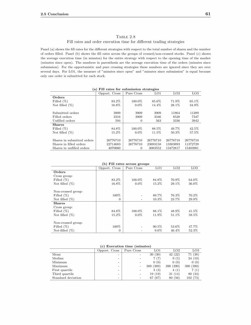
2.5 Conclusion 61
Table 2.8Fill rates and order execution time for different trading strategies
Panel (a) shows the fill rates for the different strategies with respect to the total number of shares and the number
of orders filled. Panel (b) shows the fill rates across the groups of crossed/non-crossed stocks. Panel (c) shows
the average execution time (in minutes) for the entire strategy with respect to the opening time of the market
(minutes since open). The numbers in parenthesis are the average execution time of the orders (minutes since
submission). For the opportunistic and pure crossing strategies these numbers are ignored since they are over
several days. For LO1, the measure of ”minutes since open” and ”minutes since submission” is equal because
only one order is submitted for each stock.
(a) Fill rates for submission strategies
Opport. Cross Pure Cross LO1 LO2 LO3OrdersFilled (%) 83.2% 100.0% 85.6% 71.9% 65.1%Not filled (%) 16.8% 0.0% 14.4% 28.1% 34.9%
Submitted orders 3909 3909 3909 11864 11289Filled orders 3316 3909 3346 8528 7347Unfilled orders 594 0 563 3336 3942SharesFilled (%) 84.8% 100.0% 88.5% 49.7% 42.5%Not filled (%) 15.2% 0.0% 11.5% 50.3% 57.5%
Shares in submitted orders 26776710 26776710 26776710 26776710 26776710Shares in filled orders 22714683 26776710 23693158 13303893 11372729Shares in unfilled orders 4070060 0 3083552 13472817 15403981
(b) Fill rates across groups
Opport. Cross Pure Cross LO1 LO2 LO3OrdersCross group:Filled (%) 83.2% 100.0% 84.8% 70.9% 64.0%Not filled (%) 16.8% 0.0% 15.2% 29.1% 36.0%
Non-crossed group:Filled (%) 100% - 89.7% 76.3% 70.2%Not filled (%) 0 - 10.3% 23.7% 29.9%SharesCross group:Filled (%) 84.8% 100.0% 88.1% 48.9% 41.5%Not filled (%) 15.2% 0.0% 11.9% 51.1% 58.5%
Non-crossed group:Filled (%) 100% - 90.5% 53.6% 47.7%Not-filled (%) 0 - 9.6% 46.4% 52.3%
(c) Execution time (minutes)
Opport. Cross Pure Cross LO1 LO2 LO3Mean - - 30 (30) 42 (22) 71 (38)Median - - 7 (7) 9 (5) 24 (10)Minimum - - 0 (0) 0 (0) 0 (0)Maximum - - 389 (389) 390 (390) 390 (390)First quartile - - 3 (3) 4 (1) 7 (1)Third quartile - - 19 (19) 31 (14) 80 (34)Standard deviation - - 67 (67) 80 (56) 102 (73)

62 Chapter 2 Equity Trading by Institutional Investors
In addition, the costs of alternative, more traditional, submission strategies can beestimated and compared.
By calculating several measures of liquidity for the different groups of stocks in thedata set, we show that there are significant differences in liquidity between stocks thatare crossed and stocks that have to be bought in the market. For one trading date,spreads were significantly different even though the trading volume in the two groups ofstocks was similar. According to the market microstructure literature, this might be anindication of informed trading in the stocks that could not be executed in the crossingnetwork, a result which is also suggested in Næs and Ødegaard (2000). We also find,however, that there are systematic differences in liquidity between the two groups ofstocks on other dates than the trading dates of the actual crossing strategy. This resultsuggests that there are systematic differences in the characteristics of the two groups ofstocks that are not related to private information.
To evaluate the performance of the actual crossing strategy against other submissionstrategies, we perform limit order simulations on transactions data from the NYSE. Thesimulations can also be viewed as an additional measure of trading difficulty. The non-crossed orders turn out to be significantly more expensive than the crossed orders acrossall simulations. Hence, the stocks that the Fund could not get in the crossing networkwould also have been the most difficult to buy in the market. We also show that itwould have been very hard to beat the actual opportunistic crossing strategy. Theonly simulation which gives us a lower implicit cost estimate is when we completelyignore the size of our orders. However, the explicit cost differential between the crossingnetwork and regular market would probably even this difference out. Finally, it shouldbe stressed that the significant differences found in crossing probability, liquidity andprimary market execution costs are for the 500 largest and most liquid stocks in the USmarket.

2.A Data issues and variable description 63
2.A Data issues and variable description
Calculation of liquidity and activity measures
To calculate the liquidity statistics in the primary market for all securities traded by thefund we use the TAQ database (NYSE Trades and Quotes database). However, beforewe perform the calculations, the data has to be filtered to remove erroneous recordsboth in the quotes file and the trades file.
Data issues and filtering
Quotes data
All the spread measures are calculated with respect to the inside quotes (best bid andask) reported in the TAQ database between 9:30 and 16:00. There are several filtersapplied to ”clean” the data. We mainly use the quote conditions (MODES) in the TAQdata35 to do this. An observation is removed if one of the following conditions applies;
• Closing quote The last quote from a participant during the trading day (Mode=3)
• News dissemination A regulatory halt when price sensitive news arrives (Mode=4)
• Fast trading Indicating that there is extreme activity (quotes are entered on a”best efforts” basis) making the time stamps unreliable (Mode=5)
• Order imbalance A non-regulatory trading halt due to large order imbalances(Mode=7)
• Non-firm quote A regulatory halt when the Exchange is unable to collect, pro-cess and disseminate quotes that accurately reflect market conditions (Mode=9)
• News pending A regulatory trading halt or delayed opening due to an expectednews announcement (Mode=11)
• Trading halt due to related security A non-regulatory halt used when thereis news related to one security which will affect the trading and price in anothersecurity (Mode=13)
In addition we remove quotes where the bid price is larger than the ask price, quotesare negative, or the average quoted spread is zero over the trading day. Also quoteswith a price higher than USD 10,000 are removed both due to possible errors as wellas to remove securities with extreme prices which could affect our statistics. Lastly,when quotes from several different exchanges are reported at the same time (down to
35A more detailed description can be found in the TAQ User Guide which can be downloaded fromthe NYSE homepage at http://www.nyse.com/marketinfo/marketinfo.html
64 Chapter 2 Equity Trading by Institutional Investors
the second), we use the lowest ask or highest bid among these as a proxy for the NBBO(National Best Bid and Offer).
Trades data
The trades reported in TAQ may contain corrections and errors. If so, the record hasa Correction Indicator (Corr) attached to it. The requirement is that a trade musthave a correction value less than 2 (Corr < 2). If Corr=0, then the trade record is aregular trade that was not corrected, changed, cancelled or was erroneous. If Corr=1,then the observation was later corrected, but the record contains the original time andthe corrected data for the trade. If Corr > 2, then the record is either out of timesequence, cancelled due to error or cancelled due to wrong timestamp. Thus, we removeall records with Corr ≥ 2.
There are also Sale Conditions (Corr) connected to each trade. We apply a filterremoving records with conditions that make the timing and reliability of the recordsquestionable. A record is removed if one of the following conditions applies;
• Bunched sold A bunched trade not reported within 90 seconds of execution(Cond=G)
• Sold last A trade reported later than the actual transaction time (Cond=L)
• Opened last An opening trade with delayed reporting (Cond=O)
• Sellers option Delivery date is between 2 and 60 days after the trade (Cond=R)
• Pre- and Post-Market Close Trades A trade that occurred within the currenttrading day, but is executed outside of the current market hours (Cond=T)
• Sold sale A transaction that is reported to the tape at a time later than itoccurred and when other trades occurred between the time of the transaction andits report time (Cond=Z)
• Crossing session NYSE Crossing Session matches (Cond=8 and 9)
After the filtering is performed, we use the remaining quotes and trades to calculate thefollowing liquidity and activity measures.
Spread measures
Effective spreadThe effective spread takes into account the transaction prices (and accounts for the factthat many trades are executed within the quoted spread due to price improvement).The number of trades in the security, i, on date, t, is denoted by Ni,t. The index τ
2.A Data issues and variable description 65
defines the time of the day when a trade is observed, Pi,τ is the trade price, and bidi,τ
and aski,τ is the bid and ask, respectively, at the time of the trade. The first valid tradeis normalized to τ = 1. Then, for security i on date t, the average effective spread iscalculated as,
ESi,t =1
Ni,t
Ni,t∑τ=1
{2 | Pi,τ −
aski,τ + bidi,τ
2|
}The effective spread takes into account the relationship between execution price andquoted spread, and is often considered a more appropriate measure of trading coststhan quoted spreads, especially for large trades.
Quoted dollar spreadThe average quoted dollar spread is defined as the average difference between the insidequoted ask and bid for a firm over the trading day. The quoted dollar spread is calculatedwith respect to each trade observed at time τ. The inner ask and bid is defined as aski,τ
and bidi,τ respectively, and Ni,t is the total number of trades in security i during thetrading day t. Thus, the quoted dollar spread is calculated as,
QSi,t =1
Ni,t
Ni,t∑τ=1
(aski,τ − bidi,τ)
Quoted percentage spreadThe quoted percentage spread calculates the absolute spread relative to the spreadmidpoint at each valid trade record τ. Thus,
RSi,t =1
Ni,t
Ni,t∑τ
{aski,τ − bidi,τ
(aski,τ + bidi,τ)/2
}
Volume and depth measures
It is widely argued that spreads should not be examined in isolation when using it as aliquidity measure. This is because liquidity shocks both widen spreads as well as reducedepths. Furthermore, spreads may also widen as a response to adverse selection withoutliquidity necessarily decreasing. Therefore, we also look at volume and depth measures.
Trading Volume (Shares)

66 Chapter 2 Equity Trading by Institutional Investors
The total number of shares traded in security i during day t.
VOL sharesi,t =
Ni,t∑τ=1
Qi,τ
Trading volume (USD)The total dollar value of trades during day t in security i.
VOL USDi,t =
Ni,t∑τ=1
Qi,τ · Pi,τ
TradesThe total number of trades during day t in security i.
Tradesi,t =
Ni,t∑τ=1
τi
Trade sizeThe average trade size in USD 1000 on day t in security i.
Trade sizei,t =VOL USDi,t
Tradesi,t · 1000
Quoted depthThe quoted depth is calculated as average of the quoted bid and ask depths during theday t in security i,
QDi,t = (qbidi,t + qask
i,t )/2
where qbidi,t and qask
i,t is the average depth on the bid- and the ask-side respectively insecurity i on day t.
Liquidity ratios and volatility measures
Daily Liquidity RatioThe Amivest Liquidity Ratio is one type of liquidity measurement which represents thedollar value of trading associated with a one percent change in the share price. Theliquidity ratio measures the average trading volume necessary to move the price by onepercent during a trading day. We calculate the average daily liquidity ratio over the10-day period prior to the Fund’s trading date, t0. The daily liquidity ratio for security
2.A Data issues and variable description 67
i on date t is thus calculated as,
LR(D)i,t =1
10
t0−1∑t=t0−11
VOL USDi,t
|%ri,t|/1000
where |%ri,t| is the absolute ”midpoint return” over day t calculated using the bid-askmidpoints at opening and closing to avoid biases with respect to the bid-ask bounce.VOL USDi,t is the total USD trading volume in security i on date t.
Intraday Liquidity RatioTo measure liquidity on one date, we also calculate the liquidity ratio using intradaydata. To do this, we first discretisize the data to get a common time frame. Consis-tent with several other studies we use 15-minute windows, starting from 9:30am until16:00pm. Thus, we have 26 15-minute intervals during each trading day. During eachinterval, denoted by ω, we calculate the midpoint returns using the bid-ask midpointprice at the beginning (or closest to the beginning) of each window. Thus, ω ∈ [1, 26],and the average ratio for security i on date t is calculated as,
LR(I)i,t =1
26
26∑ω=1
VOL USDi,ω
|%ri,ω|/1000
where VOL USDi,ω is the total USD volume traded in security i in window ω, and|%ri,ω| is the 15-minute absolute midpoint return over window ω. Generally, the liq-uidity ratio measure assumes that there is a linear relationship between the trade sizeand price change which is not necessarily the case. In addition, the ratio is positivelycorrelated with the general price trend in the market and negatively correlated withvolatility.
Average 10-day volatilityCalculates the 10-day average volatility prior to the actual trading date (t0) as,
V(D)i,t =
√√√√ 1
10
t0−1∑t=t0−11
(ri,t − ri)2
where ri,t is the return on day t and ri is the average return over the 10-day periodprior to the actual crossing date.
Intraday volatilityWhen calculating intraday volatility, we use the same discretization as for the intradayliquidity ratio calculations described above. Thus, we calculate the volatility of 15-minute returns over the trading day, using the bid-ask midpoint price at the beginning

68 Chapter 2 Equity Trading by Institutional Investors
of each window, such that,
V(ID)i,t =
√√√√ 1
26
26∑ω=1
(ri,ω − ri,t)2
where ri,ω is the midpoint return over 15-minute window ω, and ri,t is the averagereturn over all windows during trading day t in security i.

BIBLIOGRAPHY 69
Bibliography
Amihud, Y. and Mendelson, H. (1986). Asset pricing and the bid-ask spread. Journalof Financial Economics, 17:223–249.
Amihud, Y., Mendelson, H., and Lauterbach, B. (1997). Market microstructure andsecurities values: Evidence from the tel aviv stock exchange. Journal of FinancialEconomics, 45:365–390.
Angel, J. (1994). Limit versus market orders. Unpublished Working Paper, School ofBusiness Administration, Georgetown University.
Angel, J. J. (1997). Who gets price improvement on the NYSE? Working Paper FINC-1377-12-694, Georgetown University.
Bacidore, J. M., Ross, K., and Sofianos, G. (1999). Quantifying best execution at theNew York Stock Exchange: Market orders. NYSE Working Paper 1999-05.
Barclay, M. J. and Hendershott, T. (2002). Price discovery and trading costs afterhours. Working Paper, University of Rochester, Forthcoming in Review of FinancialStudies.
Barclay, M. J., Hendershott, T., and McCormick, D. T. (2001). Electronic communica-tions networks and market quality. Working Paper, University of Rochester.
Biais, B., Hillion, P., and Spatt, C. (1995). An empirical analysis of the limit orderbook and the order flow in the Paris Bourse. Journal of Finance, 50:213–231.
Chakrevarty, S. and Holden, C. (1995). An integrated model of market and limit orders.Journal of Financial Intermediation, 4:213–241.
Cho, J. W. and Nelling, E. (2000). The probability of limit order execution. FinancialAnalysts Journal, 56:28–33.
Chordia, T., Roll, R., and Subrahmanyam, A. (2001). Market liquidity and tradingactivity. Journal of Finance, 56:501–30.
Chowdhry, B. and Nanda, V. (1991). Multi–market trading and market liquidity. Reviewof Financial Studies, 4:483–511.
Conrad, J., Johnson, K. M., and Wahal, S. (2001a). Institutional trading and softdollars. Journal of Finance, 56:397–416.
Conrad, J., Johnson, K. M., and Wahal, S. (2001b). Institutional trading costs andalternative trading systems. Working Paper, University of North Carolina at ChapelHill, Forthcoming in Journal of Financial Economics.
Coppejeans, M. and Domowitz, I. (1999). Pricing behavior in an off-hours computerizedmarket. Working Paper, Pennsylvania State University.
Domowitz, I. (2001). Liquidity, transaction cost and reintermediation in electronicmarkets. eBusiness Research Center Working Paper 4-2001, Penn State University.

70 Chapter 2 Equity Trading by Institutional Investors
Domowitz, I. and Steil, B. (1998). Automation, trading costs and the structure of thetrading services industry. Working Paper, Penn State University.
Donges, J. and Heinemann, F. (2001). Competition for order flow as a coordinationgame. Working paper No. 64, Goethe-Universitat Frankfurt.
Easley, D., Kiefer, N. M., and O’Hara, M. (1996a). Cream-skimming or profit sharing?The curious role of purchased order flow. Journal of Finance, 51:811–833.
Easley, D., Kiefer, N. M., O’Hara, M., and Paperman, J. B. (1996b). Liquidity, infor-mation, and infrequently traded stocks. Journal of Finance, 51:1405–1436.
Easley, D. and O’Hara, M. (1992). Time and the process of security price adjustment.Journal of Finance, 47:577–606.
Fong, K., Madhavan, A., and Swan, P. (1999). Why do securities markets fragment?Working Paper, University of Southern California.
Foucault, T. (1999). Order flow composition and trading costs in a dynamic limit ordermarket. Journal of Financial Markets, 1(2):99–134.
Glosten, L. (1994). Is the electronic open limit order book inevitable? Journal ofFinance, 49:1127–1161.
Handa, P. and Schwartz, R. A. (1996). Limit order trading. Journal of Finance, 51:1835–1861.
Harris, L. (1990). Liquidity, trading rules, and electronic trading systems. New YorkUniversity Salomon Center Monograph Series in Finance and Economics, 4.
Harris, L. (2002). Trading and Exchanges. Market Microstructure for Practitioners.Oxford University Press.
Harris, L. and Hasbrouck, J. (1996). Market vs. limit orders: The superDOT evidenceon order submission strategy. Journal of Financial and Quantitative Analysis, 31:231–231.
Hasbrouck, J. and Saar, G. (2001). Limit orders and volatility in a hybrid market: Theisland ECN. Stern Working Paper, New York University.
Hendershott, T. and Mendelson, H. (2000). Crossing networks and dealer markets:Competition and performance. Journal of Finance, 55:2071–2115.
Hollifield, B., Miller, R., and Sandas, P. (1999). An empirical analysis of a pure limitorder market. Working Paper 029-99, University of Pennsylvania.
Jones, C. M. and Lipson, M. L. (1999a). Execution costs of institutional equity orders.Journal of Financial Intermediation, 8:123–140.
Jones, C. M. and Lipson, M. L. (1999b). Sixteenths: Direct evidence on institutionalexecution costs. Working Paper, Columbia Business School.
Keim, D. B. and Madhavan, A. (1995). Anatomy of the trading process: Empiricalevidence for the motivation for and execution of instituional equity trades. Journalof Financial Economics, 37:371–398.
BIBLIOGRAPHY 71
Keim, D. B. and Madhavan, A. (1997). Transactions costs and investment style: Aninter-exchange analysis of institutional equity trades. Journal of Financial Economics,46:265–292.
Keim, D. B. and Madhavan, A. (1998). The cost of institutional equity trades. FinancialAnalysts Journal, 54:50–69.
Khan, W. A. and Baker, H. K. (1993). Unlisted trading privileges, liquidity, and stockreturns. Journal of Financial Research, 16:221–236.
Lo, A. W., MacKinlay, A. C., and Zhang, J. (2002). Econometric models of limit-orderexecutions. Journal of Financial Economics, 65:31–71.
Mendelson, H. (1987). Consolidation, fragmentation, and market performance. Journalof Financial and Quantitative Analysis, 22:189–207.
Næs, R. and Ødegaard, B. A. (2000). Equity trading by institutional investors. To crossor not to cross? Discussion Paper 3/2000, Norwegian School of Management BI.
Parlour, C. (1996). Price dynamics in limit order markets. Mimeo, Carnegie-MellonUniversity.
Perold, A. (1988). The implementation shortfall: Paper versus reality. Journal ofPortfolio Management, 14(3):4–9.
Ruyter, T. (1999). The dinosaur, the rock, and the hard place. Plan Sponsor.
Seppi, D. (1990). Equilibrium block trading and asymmetric information. Journal ofFinance, 45:73–94.
Seppi, D. (1997). Liquidity provision with limit orders and a strategic specialist. Reviewof Financial Studies, 10:103–150.
Treynor, J. L. (1981). What does is take to win the trading game? Financial AnalystsJournal, 47(1).

72
Chapter 3
Order Book Characteristics and
the Volume-Volatility Relation:
Empirical Evidence from a Limit
Order Market
Written with Randi Næs
Abstract
We examine empirically the relationship between the demand and supply schedulesin a limit order book and the volume volatility relation. Several empirical studiesfind support for the hypothesis that the volume-volatility relation is driven by thearrival rate of new information, proxied by the number of transactions. Our resultsshow that the number of trades and the price volatility are also related to the slopeof the order book. One possible interpretation for this finding is that the slope ofthe book is proxying for dispersed beliefs among investors. If so, this would supportmodels where investor heterogeneity intensifies the volume-volatility relation.
73

74 Chapter 3 Order Book Characteristics and the Volume-Volatility Relation
3.1 Introduction
In this paper, we examine empirically the relationship between the demand and supplyschedules in a limit order book and the volume volatility relation.
A variety of studies document that there is a positive correlation between pricevolatility and trading volume for most types of financial contracts including stocks,Treasury bills, currencies and various futures contracts. The main theoretical explana-tion for this phenomenon is that new information about asset values acts as the drivingforce (or mixing variable) for both market prices and trading volume. Harris (1986) linksthis “mixture of distributions hypothesis” to asset pricing theory, and suggests that themixing variable is the process that directs the rate of flow of information from system-atic risk factors into prices and trading volume. However, for many types of financialcontracts, movements in prices seem much “too large” to be attributed to movementsin the fundamental values of the underlying securities.1 A suggested explanation forthis puzzle is that prices do not change merely because of changes in systematic riskfactors and asset payoffs but also because investors have dispersed beliefs about assetvalues. This dispersion may be due to asymmetric information or to differences of opin-ion about symmetric information. In any case, theoretical models by Shalen (1993)(asymmetric information) and Harris and Raviv (1993) (symmetric information) showthat dispersion of beliefs will intensify the volume-volatility relation, by increasing bothtrading volume and volatility.
The theoretical explanations for the volume-volatility relation are hard to test. Theessence of the mixture of distributions hypothesis is that prices adjust to new equilibriaover time as new information is being reflected through trades. Since the arrival rateof information is unobservable, it is difficult to set up an alternative hypothesis. Sev-eral empirical studies find support for the explanation under the assumption that thearrival rate of information can be proxied by the daily number of transactions.2 Sincethe daily number of transactions may be driven by factors other than new information,these studies do not rule out the other explanations for the volume-volatility relation.Specifying data implications from the models with dispersed beliefs is also very chal-lenging. Daigler and Wiley (1999) perform an indirect test of Shalen (1993)’s modeland find evidence that uninformed traders contribute to price volatility. Ghysels andJuergens (2001) measure dispersion of beliefs directly by dispersion of analysts’ earningsforecasts. They also find that dispersion is positively related to volatility.
The objective of this paper is to broaden our knowledge about the volume-volatilityrelation in an electronic limit order market. Since the demand and supply schedules in alimit order book represent the reservation prices of the liquidity suppliers in the market,it is interesting to study whether the book contains additional information about the
1A standard reference for the stock market is Shiller (1981).2See Harris (1987) and Jones et al. (1994)
3.1 Introduction 75
volume-volatility relation. We have access to exceptionally rich transactions data fromthe Norwegian equity market in the period from February 1999 through June 2001. Themarket operates as a fully automated limit order-driven trading system, and our datasample enables us to rebuild the full order book at any point in time. We are not awareof anyone who has investigated this issue with a data set as rich as ours.
Several papers investigating order book data are relevant for our work. Biais et al.(1995) analyze in detail the interaction between the order book and order flow on theParis Bourse. One relevant finding is that the status of the order book is important fororder flows and trading volume. Biais et al. (1995) only have data on the cumulativetrading interest near the inner quotes. We show that the whole order book containsadditional, interesting information. Goldstein and Kavajecz (2000) provide evidence ofa negative relation between the shape of the order book and volatility during a caseof an extreme market movement. However, they do not attempt to investigate thisrelation over a longer time period with varying trading conditions. Our data set spansa relatively long period which included the boom and burst of the internet bubble.Kalay et al. (2003) estimate the demand and supply elasticities for stocks on the TelAviv Stock Exchange. Their main findings are that the order book is more elastic atthe beginning of the day, and that the demand side is more elastic than the bid side.3
Kalay et al. (2003) only have data for order placements at the opening of the market.Our estimates of supply and demand schedules are also based on the continuous tradingsession.
We first establish that the standard volume-volatility relation exists in a limit ordermarket, and investigate in detail the composition of the order book at the intra-day level.This exercise documents that the trading structure on the Norwegian Stock Exchangeexhibits the same features as are found in empirical studies of other countries’ stockmarkets. The features suggest that: informational asymmetries are more pronouncedat the beginning of the trading day, there is competition among informed traders, anduninformed traders require a compensation for the higher pick-off risk at the beginningof the day.4 These results are systematic across sub-periods, firm sizes, and tick-sizes.
The main contribution of our study is that we are able to document several rela-tionships between the volume-volatility relation and the shape of the order book. Wemeasure the order book shape by the average elasticity of the supply and demand sched-ules in the book. The lower the elasticity (steeper the slope), the less dispersed are thebid and ask prices in the order book.5 To examine the effects of the order book slope on
3The first result is interpreted as supportive to sequential trading models with asymmetric informa-tion which predict higher adverse selection at the opening (Glosten and Milgrom, 1985). The secondresult is interpreted as supportive to the empirical finding that buy orders have larger price impactsthan sell orders.
4Our results are in accordance with the results in Kalay et al. (2003) as well as with the results inseveral studies of time-of-day effects in spreads and price impacts, for example French and Roll (1986),Harris (1986), and Niemeyer and Sandas (1995).
5This is in the case of direct demand and supply curves (prices on the x-axis and accumulated volume

76 Chapter 3 Order Book Characteristics and the Volume-Volatility Relation
volume and volatility, we first include the slope measure as an independent variable ina cross sectional time series version of the standard regression model used to documentthe volume-volatility relation. To investigate the relationship between the slope of thebook and the trading activity, we estimate a cross-sectional time series regression withthe number of trades as the dependent variable. A systematic negative relation betweenthe average slope of the order book and the price volatility is documented in a dailytime series cross-sectional analysis. These results are also shown to be robust to thechoice of time period. Similarly, we find a significant and robust negative relationshipbetween our slope measure and the daily number of trades.
If the slope of the book is essentially a liquidity measure, most of the informationcontained in the slope should be reflected by the volume close to the inner quotes. Tocheck this, we calculate the slope measure based on different fractions of the order bookand re-estimate all the regression models. When we investigate the relation betweendifferent slope measures and trading activity, an interesting pattern emerges. In linewith the findings in Biais et al. (1995) that thick books at the inner quotes result intrades, we find a significant positive relationship between the slope of the book and thenumber of trades when the slope is calculated based on the volume at the inner quotes.This result is the opposite of what we get when we use a slope measure based on thefull order book. Thus, the slope of the book provides different information dependingon what fraction of the book we use in the calculation.
A possible interesting interpretation of the full order book slope is related to thedispersion of beliefs hypothesis. Harris (1987) notes that, if trades are self generating,the number of daily transactions will be the true mixing variable rather than a proxyfor the arrival rate of new information. It could be that the slope of the limit orderbook capture dispersion of beliefs about asset values, i.e. steep slopes of the supply anddemand schedules indicate that there is a high degree of agreement among investorsabout the fair value of the security, while gentle slopes indicate that there is greaterdisagreement among investors about the value of the security. If so, our finding thatthere is increased trading activity when slopes are more gentle (greater disagreementabout valuation) could reflect a situation of self generating trades, i.e. that the volume-volatility relation is not merely driven by new information. This interpretation wouldbe in line with models where heterogeneity among investors contributes to the volume-volatility relation.
On the other hand, our results can also be explained within a Glosten (1994) typeof model where all liquidity suppliers are homogeneous: for a given level of liquiditymotivated trading and a given probability of informed trading, the slopes will be moregentle the more volatile assets are, while a positive relation between the slope at the
on the y-axis). In the case of inverted demand and supply curves, the relationship would be opposite.

3.2 Literature 77
inner quotes and trading activity could be explained by price sensitive liquidity traders.6
However, the results from the test of the Glosten model in Sandas (2001) do not provideempirical support for a model with homogeneous liquidity suppliers.
The paper is organized in the following way. Section 3.2 surveys the relevant liter-ature. Section 3.3 describes our data sample. Section 3.4 examines in detail the orderflow and order book on an intra-daily basis. Section 3.5 provides the results from ouranalysis of the volume-volatility relation in the Norwegian equity market. Section 3.6concludes the paper.
3.2 Literature
The mixture of distributions hypothesis The early research into the volume-volatility relation is reviewed in Karpoff (1987). The main theoretical explanation fromthis period is known as the “mixture of distributions hypothesis” (hereafter the MDH).According to the MDH, there is a positive correlation between daily price changesand trading volume because both variables are mixtures of independent normals withthe same mixing variable. Originally, the MDH was suggested by Clark (1973) asan alternative explanation for the observed leptokurtosis in the distribution of log pricechanges.7 The basic idea underlying the hypothesis is that prices and trading volume aredriven by a time-varying arrival rate of information.8 Let ∆pi,t and vi,t be respectivelythe intraday price change and volume of trade resulting from information event numberi on date t, and let nt be the total number of information events during day t. Assumethat (i) the number of events each day, nt, varies across days, and that (ii) the intradayprice changes, ∆p, and trading volumes, v, are jointly independently and identicallydistributed with finite variances. Our explanation of the MDH is largely based onHarris (1987). The daily price change and trading volume are equal to the sum ofrespectively the intraday price changes and trading volumes, i.e.
∆Pt =
nt∑i=1
∆pi,t and Vt =
nt∑i=1
vi,t (3.1)
6We are grateful to an anonymous referee for pointing this out to us.7Mandelbrot (1963) and Fama (1963) showed that the return distributions of commodity and stock
prices were leptokurtic, and well approximated by symmetric stable distributions with characteristicexponents between 1 and 2 (the normal distribution has a characteristic exponent equal to 2). Anexamination of the stable distributions hypothesis for the Norwegian market is provided in Skjeltorp(2000) who shows that a characteristic exponent between 1.6 and 1.7 best characterizes the Norwegiandata.
8Copeland (1976, 1977)’s “sequential arrival of information” model which is later extended by Jen-nings et al. (1981) and Jennings and Barry (1983) also predicts a positive relationship between volumeand absolute price changes. The main feature of the model is that information is disseminated to onlyone trader at a time, and the main criticism of the models is that traders cannot learn from the marketprices as other traders become informed.
78 Chapter 3 Order Book Characteristics and the Volume-Volatility Relation
where ∆Pt is the daily price change and Vt is the daily trading volume. Given equa-tion (3.1), and provided that nt is large, the joint distribution of the daily price changeand volume of trade will be approximately bivariate normal conditional on nt.9 Thevolume-volatility relation arises because both price changes and trading volume arelikely to be large when the number of information events is large and small when thenumber of information events is small.10
Harris (1986) finds empirical support for the MDH based on cross-sectional tests ofcommon stocks continuously traded on the NYSE or one of the regional exchanges inthe period 1976-1977. The critical assumption behind the tests is that the distributionof the mixing variable is not identical for all securities. Assuming that transactions takeplace at a uniform rate in event time, Harris (1987) finds both theoretical motivationand empirical support for the use of the daily number of transactions as a proxy forthe time-varying unobserved information evolution rate.11 However, since the arrivalrate of new information is unobservable, we do not know whether a part of the volume-volatility relation may be a result of the actions of heterogeneous traders. As suggestedby Harris (1987), if trading is self-generating, the daily number of transactions would bethe true mixing variable rather than a proxy for the unobserved information evolutionrate.
Using a simple regression approach for daily data on Nasdaq-NMS securities overthe 1986-1991 period, Jones et al. (1994) find that both volatility and trading volumeare positively correlated with the number of daily transactions. However, the averagesize of trades contains no additional information about volatility beyond that containedin the number of transactions. If the number of transactions is a good proxy for themixing variable, this result is supportive of a pure MDH; “..volatility and volume arepositively correlated only because both are positively related to the number of dailyinformation arrivals (the mixing variable).” The problem caused by a lack of abilityto interpret the mixing variable can be further illustrated by this study. If informedtraders camouflage their information, for example by splitting their orders into mediumsized trades as suggested by the “stealth trading hypothesis” of Barclay and Warner(1993), the number of daily transactions would be the true mixing variable and theresults in Jones et al. (1994) would also support explanations of the volume-volatilityrelation based on heterogeneous traders.12
9See Harris (1987), page 129.10The variation in the daily number of information events implies that the expectation of the uncon-
ditional distribution is a weighted average (or “a mixture”) of the conditional distributions.11Harris (1987) derives and tests several implications of the MDH for transactions data on a sample
of 50 NYSE stocks that traded between December 1, 1981 and January 31, 1983. The results from thetests are supportive of the MDH.
12In addition, in order-driven markets, a large order is often automatically executed against manysmaller orders by the automatic matching system. Thus, even though the original order is large, it mayshow up as many small trades as it is matched against several smaller orders rendering the average dailytrade size unimportant in explaining volatility.
3.2 Literature 79
Dispersion of belief The MDH simply states that price changes and trading volumeare directed by the flow of new information. It does not say anything about what type ofinformation or how this information is revealed to investors. Hence, an important limi-tation of the hypothesis is that it does not address the role of economic agents or marketstructure for prices and trading volume. Later theoretical work on the volume-volatilityrelation centers around these issues. Harris (1986) links the MDH to asset pricing the-ory by suggesting that the mixing variable directs the rate of flow of information fromsystematic risk factors. A problem with this interpretation is that the movements inprices for many types of financial contracts seem much “too large” to be attributed tomovements in the fundamental values of the underlying securities only. This fact sug-gests that prices are not merely driven by changes in systematic risk factors and assetpayoffs, but also by changes in the expectations of heterogeneous agents. Figure 3.1illustrates the information structure in a standard asset market for the two main typesof such models. Panel (a) in the figure describes a “differences in opinion” model, whilepanel (b) describes a market microstructure model with asymmetric information.
Figure 3.1 (a) illustrates a “differences of opinion” model. In this model, investorsare assumed to act differently on the same news, i.e. trading is induced by differencesof opinion about publicly available information. Beliefs are updated using Bayes rule.All traders are rational, but they view others as having irrational models. Harris andRaviv (1993) explain the volume-volatility relation by a model of this kind. Two groupsof risk-neutral speculators receive the same information but disagree on the extent towhich it is important (but agree to disagree). As long as one of the groups remainsmore optimistic than the other, there is no trading. Trading occurs only and wheneverthe cumulative information for one of the trader groups switches from favorable tounfavorable, or vice versa.13
In the standard asset pricing models, the trading process itself does not conveyinformation which is relevant to price determination. Prices adjust immediately as aresult of new information. This is a plausible assumption for some kind of news. Othertypes of news are likely to be dispersed and not immediately available to all investorsin aggregated form.14 Modelling dispersed information is the essential feature in themarket microstructure models illustrated in figure 3.1 (b). In these models, there is agroup of investors who trade on the basis of private information. The market maker andthe uninformed investors can only infer this information from trades and order flows.The room for strategic behavior among agents differs in different models.15 Shalen
13Prices change every period whether or not trading occurs. The volume-volatility relation arisesbecause the price changes are larger on average when trading occurs.
14Evidence of the existence of dispersed news is given in French and Roll (1986) who documentempirically that asset prices are much more volatile during exchange trading hours than during non-trading hours. This phenomenon cannot be reconciled with a standard asset pricing model unless thereis a systematic tendency for price-relevant information to arrive during normal business hours only.
15In Kyle (1985), informed investors attempt to camouflage their trades by spreading them over time.
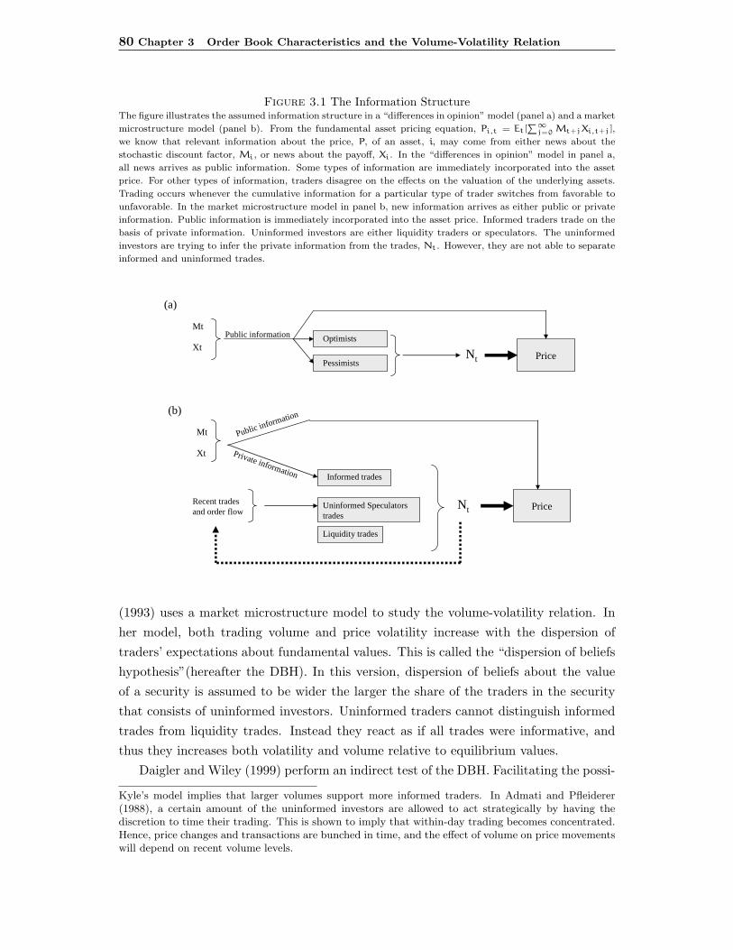
80 Chapter 3 Order Book Characteristics and the Volume-Volatility Relation
Figure 3.1 The Information StructureThe figure illustrates the assumed information structure in a “differences in opinion” model (panel a) and a market
microstructure model (panel b). From the fundamental asset pricing equation, Pi,t = Et[∑∞
j=0 Mt+jXi,t+j],
we know that relevant information about the price, P, of an asset, i, may come from either news about the
stochastic discount factor, Mi, or news about the payoff, Xi. In the “differences in opinion” model in panel a,
all news arrives as public information. Some types of information are immediately incorporated into the asset
price. For other types of information, traders disagree on the effects on the valuation of the underlying assets.
Trading occurs whenever the cumulative information for a particular type of trader switches from favorable to
unfavorable. In the market microstructure model in panel b, new information arrives as either public or private
information. Public information is immediately incorporated into the asset price. Informed traders trade on the
basis of private information. Uninformed investors are either liquidity traders or speculators. The uninformed
investors are trying to infer the private information from the trades, Nt. However, they are not able to separate
informed and uninformed trades.
PriceXt
OptimistsPublic information
Nt
Mt
Pessimists
Price
Xt
Recent trades and order flow
Informed trades
Uninformed Speculatorstrades
Liquidity trades
Private information
Nt
Mt
(a)
(b)
Public information
(1993) uses a market microstructure model to study the volume-volatility relation. Inher model, both trading volume and price volatility increase with the dispersion oftraders’ expectations about fundamental values. This is called the “dispersion of beliefshypothesis”(hereafter the DBH). In this version, dispersion of beliefs about the valueof a security is assumed to be wider the larger the share of the traders in the securitythat consists of uninformed investors. Uninformed traders cannot distinguish informedtrades from liquidity trades. Instead they react as if all trades were informative, andthus they increases both volatility and volume relative to equilibrium values.
Daigler and Wiley (1999) perform an indirect test of the DBH. Facilitating the possi-
Kyle’s model implies that larger volumes support more informed traders. In Admati and Pfleiderer(1988), a certain amount of the uninformed investors are allowed to act strategically by having thediscretion to time their trading. This is shown to imply that within-day trading becomes concentrated.Hence, price changes and transactions are bunched in time, and the effect of volume on price movementswill depend on recent volume levels.

3.2 Literature 81
bility of distinguishing traders with different types of information in the futures markets,they test whether uninformed traders contribute to volatility. The results of their studysupport Shalen (1993): “..uninformed traders who cannot differentiate liquidity demandfrom fundamental value increase volatility.” In a similar study, Bessembinder and Seguin(1993) examine the relation between the volume-volatility relation and market depth,proxied by open interest, in eight physical and financial futures markets. Unexpectedvolume is found to have a larger effect on volatility than expected volume, and largeopen interest is found to mitigate volatility.
Limit order markets In this paper, we investigate the information about tradingvolume and price volatility contained in the slope of a limit order book. In an electroniclimit order market, liquidity is not supplied by designated specialists or market makers,but rather by the traders themselves. The majority of trades are first submitted to themarket as limit orders, which accumulate into the limit order book. Hence, at any pointin time, the limit order book reflects an aggregate of buying and selling interests atvarious prices. Each ask (bid) price reflects the lowest (highest) price at which differentinvestors are willing to sell (buy) the security.16
Theoretical models of limit order markets differ in their assumptions about investorheterogeneity. In Glosten (1994), privately informed investors are assumed to submitmarket orders while homogeneous uninformed investors provide the limit order book.Hence, the shape of the limit order book reflects the information characteristics of theincoming market flow. In the dynamic model proposed by Parlour (1998), all tradersare assumed to have different valuations for the traded asset. Parlour shows that, whenthe choice between a limit order or a market order depends both on the past (throughthe state of the order book) and the future (through expected subsequent order flow),then systematic patterns in order placement strategies will be generated even in theabsence of asymmetric information. Moreover, both sides of the book will matter foroptimal order placement strategies. Foucault et al. (2003) model a limit order marketwhere liquidity suppliers have asymmetric information on the risk of being picked off bytraders with superior information. This feature is shown to affect the shape of the orderbook. When the book is thin, uninformed liquidity traders are reluctant to add depthbecause it may be an indication of high pick-off risk. The informed liquidity tradersexploit this by bidding less aggressively than in the case where the liquidity traders havesymmetric information. Sandas (2001) tests a version of Glosten (1994) empirically.17
16Biais et al. (1995) note that the shape of the order book may reflect the competition among buy-ers/sellers as well as the correlation in their valuations. If the supply and demand curves are inelasticand volume is concentrated around the inner quotes, this may reflect that the valuations among variousinvestors are correlated on each side of the market relative to the case where the valuations are moredispersed and the order book is more elastic.
17The tests are based on updating restrictions that link the market order flow to the order bookdynamics and break-even conditions for the marginal bid and offer prices that define the price schedule.
82 Chapter 3 Order Book Characteristics and the Volume-Volatility Relation
The results do not lend support to the model. Relative to the theoretical predictions,the empirical price schedules of the limit order book offer insufficient depth.
3.3 The Data
3.3.1 The Norwegian Stock Market
Our data set is from the the Oslo Stock Exchange (OSE) in Norway.18 Norway isa member of the European Economic Area, and its equity market is among the 30largest world equity markets by market capitalization.19 Table 3.1 reports some generalstatistics for all the companies listed on the OSE. At the end of 2001, 212 firms werelisted on the exchange with a total market value of about NOK 657 bill. The OSE isthe only regulated marketplace for securities trading in Norway. Since January 1999, ithas operated as a fully computerized centralized limit order book system similar to thepublic limit order book systems in e.g. Paris, Toronto, Stockholm and Hong Kong.
The OSE allows the use of limit orders, market orders, and various customary orderspecifications. Participants can also submit hidden orders. When an order is submittedas a hidden order, only a specified fraction of the underlying order is visible to themarket. As is normal in most electronic order-driven markets, the order handling rulefollows a strict price-time priority.20 All orders are submitted at prices constrained bythe minimum tick size for the respective stocks which is determined by the price levelof the stock. For prices lower than NOK 9.99 (Norwegian kroner) the tick size is NOK0.01, between NOK 10 and NOK 49.9 the tick size is NOK 0.1, between NOK 50 andNOK 999.5 the tick size is NOK 0.5 and for prices above NOK 1000 the tick size isNOK 1.
The trading day of the OSE comprises two sessions: the “pre-trade” session startingat 9:30 and ending with an opening auction at 10:00, and the “continuous trading”session from 10:00 until the trading closes at 16:00. During the pre-trade session, brokerscan register trades that were executed after the close on the previous day as well as neworders. At the opening auction at the end of the pre-trade session, all orders registeredin the order book are automatically matched if the prices are crossing or equal. Thequoted opening price is thus the price that clears the market. During the continuoustrading session, electronic matching of orders with crossing or equal price generatestransactions. Orders without a limit price (market orders) have automatic price priorityand are immediately executed at the best available prices. At the OSE, market orders
18We obtained the data directly from the exchange’s surveillance system. The SMARTS c© systemis the core of the exchange’s surveillance operations. Through access to the SMARTS c© database, weobtained all the information on orders and trades in the market
19Source is FIBV (International Federation of Stock exchanges). Notable Norwegian listings includeNorsk Hydro, Telenor, and Statoil.
20In the case of hidden orders, when the visible part of the order is executed, it loses time priority.
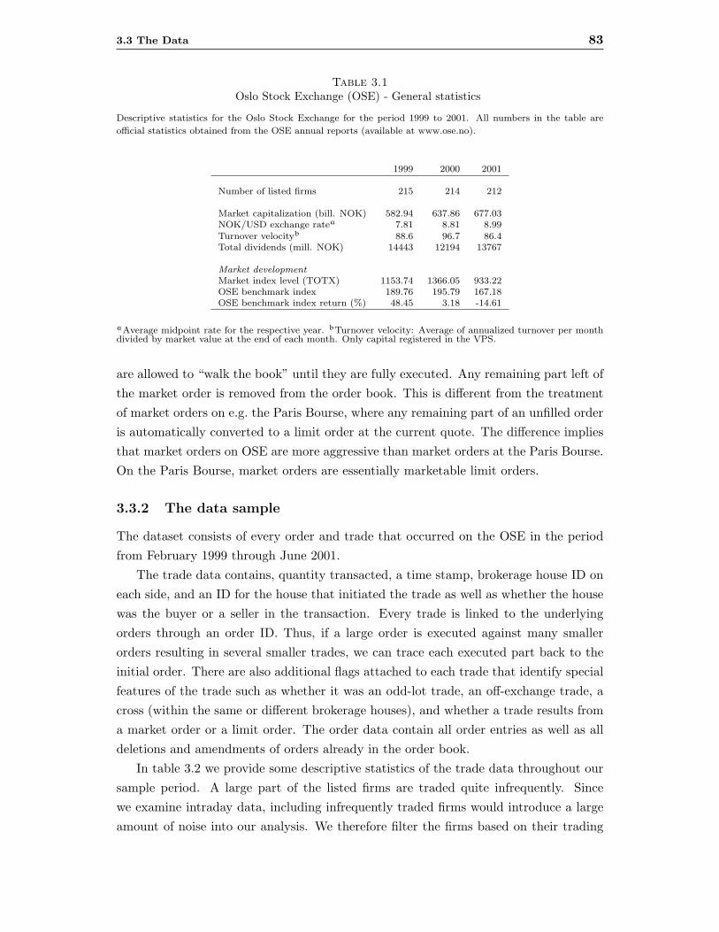
3.3 The Data 83
Table 3.1Oslo Stock Exchange (OSE) - General statistics
Descriptive statistics for the Oslo Stock Exchange for the period 1999 to 2001. All numbers in the table are
official statistics obtained from the OSE annual reports (available at www.ose.no).
1999 2000 2001
Number of listed firms 215 214 212
Market capitalization (bill. NOK) 582.94 637.86 677.03NOK/USD exchange ratea 7.81 8.81 8.99Turnover velocityb 88.6 96.7 86.4Total dividends (mill. NOK) 14443 12194 13767
Market developmentMarket index level (TOTX) 1153.74 1366.05 933.22OSE benchmark index 189.76 195.79 167.18OSE benchmark index return (%) 48.45 3.18 -14.61
aAverage midpoint rate for the respective year. bTurnover velocity: Average of annualized turnover per monthdivided by market value at the end of each month. Only capital registered in the VPS.
are allowed to “walk the book” until they are fully executed. Any remaining part left ofthe market order is removed from the order book. This is different from the treatmentof market orders on e.g. the Paris Bourse, where any remaining part of an unfilled orderis automatically converted to a limit order at the current quote. The difference impliesthat market orders on OSE are more aggressive than market orders at the Paris Bourse.On the Paris Bourse, market orders are essentially marketable limit orders.
3.3.2 The data sample
The dataset consists of every order and trade that occurred on the OSE in the periodfrom February 1999 through June 2001.
The trade data contains, quantity transacted, a time stamp, brokerage house ID oneach side, and an ID for the house that initiated the trade as well as whether the housewas the buyer or a seller in the transaction. Every trade is linked to the underlyingorders through an order ID. Thus, if a large order is executed against many smallerorders resulting in several smaller trades, we can trace each executed part back to theinitial order. There are also additional flags attached to each trade that identify specialfeatures of the trade such as whether it was an odd-lot trade, an off-exchange trade, across (within the same or different brokerage houses), and whether a trade results froma market order or a limit order. The order data contain all order entries as well as alldeletions and amendments of orders already in the order book.
In table 3.2 we provide some descriptive statistics of the trade data throughout oursample period. A large part of the listed firms are traded quite infrequently. Sincewe examine intraday data, including infrequently traded firms would introduce a largeamount of noise into our analysis. We therefore filter the firms based on their trading

84 Chapter 3 Order Book Characteristics and the Volume-Volatility Relation
activity through the sample period. The first filtering criterion is that the firm musthave been traded in at least 400 out of 597 days, or about 70 percent of the tradingdays, and the second criterion is that the firm must have an average of 5 trades per dayto be included in our sample. Once the first criterion is applied, the second criteriononly removes a few companies from our sample. After the filtering we are left with108 firms, which constitute our sample throughout the paper. Note that there were215, 214 and 212 listed firms at the end of 1999, 2000 and 2001 respectively. Table 3.2shows that there has been increasing trading activity during the sample period withthe total number of trades having tripled and the volume in Norwegian kroner (NOK)having doubled. Further, the average number of daily trades across firms has more thandoubled from 32 in the first half of 1999 to 79 in the first half of 2001.21 The increasein activity has also been accompanied by a decrease in the average percentage spread.As found in most markets, the average effective spreads are lower than the averagequoted spreads. To give a better picture of the diversity of the sample, we divide thesample into four portfolios based on their market capitalization value. The firms areassigned to a market capitalization group based on their market capitalization valueat the beginning of each year. The general picture is that the number of trades, thetrading volume (both in shares and NOK), the prices and the quoted spread increaseacross firm size portfolios, while the average daily volatility, the average trade size andthe quoted percentage spread decrease.
We also report the average correlations between the trading volume, the trade sizeand the number of transactions. The correlation structure in our sample is quite similarto the one documented for the US market in Jones et al. (1994). The correlation betweenthe average trade size and the number of trades is low, and both the average trade sizeand the number of trades have high positive correlations with share volume. Hence, thetwo components of share volume seem to contain different information about volume.The same structure is evident when we calculate correlations over sub-periods of half ayear.
3.3.3 Composition of orders
Our order data are quite rich. For each order, we have a time stamp, a unique order ID,the disclosed/hidden orders as well as flags indicating whether the order was a buy orsell order, whether the order is a new order, a deletion of an order or an amendment toan existing order (price change and/or volume change). In addition, a unique brokeragehouse ID is attached to each order. Moreover, compared to the Paris Bourse data inBiais et al. (1995), our data are not restricted to include placements, amendments and
21At the same time, the average trade size has gone down from 3429 shares to 2648 shares. Thisdecline is most likely related to the introduction and growth of online trading in the sample period,since these traders generate a lot of trades of small sizes. During our period, the fraction of total tradescoming from pure online brokerage houses has increased from 0% to almost 10%.
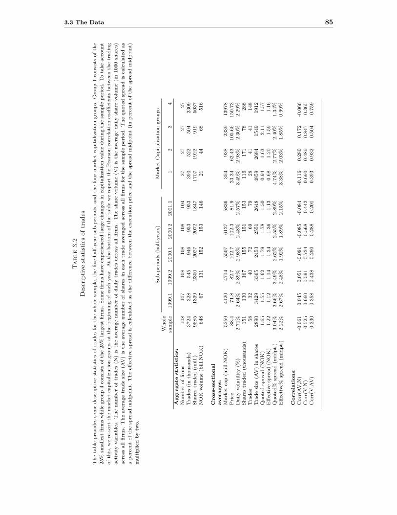
3.3 The Data 85
Table
3.2
Des
crip
tive
stat
isti
csof
trad
es
The
table
pro
vid
esso
me
des
crip
tive
stati
stic
softr
ades
for
the
whole
sam
ple
,th
efive
half-y
ear
sub-p
erio
ds,
and
the
four
mark
etca
pitaliza
tion
gro
ups.
Gro
up
1co
nsi
sts
ofth
e
25%
smalles
tfirm
sw
hile
gro
up
4co
nsi
sts
ofth
e25%
larg
est
firm
s.Som
efirm
shave
exper
ience
dla
rge
changes
inca
pitaliza
tion
valu
eduri
ng
the
sam
ple
per
iod.
To
take
acc
ount
ofth
is,w
ere
-sort
the
mark
etca
pit
aliza
tion
gro
ups
at
the
beg
innin
gofea
chyea
r.A
tth
ebott
om
ofth
eta
ble
we
report
the
Pea
rson
corr
elati
on
coeffi
cien
tsbet
wee
nth
etr
adin
g
act
ivity
vari
able
s.T
he
num
ber
of
trades
(N)
isth
eaver
age
num
ber
of
daily
trades
acr
oss
all
firm
s.T
he
share
volu
me
(V)
isth
eaver
age
daily
share
volu
me
(in
1000
share
s)
acr
oss
all
firm
s.T
he
aver
age
trade
size
(AV
)is
the
aver
age
num
ber
ofsh
are
sin
each
trade
aver
aged
acr
oss
all
firm
sfo
rth
esa
mple
per
iod.
The
quote
dsp
read
isca
lcula
ted
as
aper
cent
ofth
esp
read
mid
poin
t.T
he
effec
tive
spre
ad
isca
lcula
ted
as
the
diff
eren
cebet
wee
nth
eex
ecution
pri
ceand
the
spre
ad
mid
poin
t(in
per
cent
ofth
esp
read
mid
poin
t)
mult
iplied
by
two.
Sub-p
erio
ds
(half-y
ears
)M
ark
etC
apitaliza
tion
gro
ups
Whole
sam
ple
1999.1
1999.2
2000.1
2000.2
2001.1
12
34
Aggregate
statist
ics:
Num
ber
offirm
s108
107
108
108
108
104
27
27
27
27
Tra
des
(in
thousa
nds)
3724
328
545
946
953
953
390
522
504
2309
Share
str
aded
(mill.)
9585
1339
2300
2027
2072
1847
1707
1922
919
5037
NO
Kvolu
me
(bill.N
OK
)648
67
131
152
153
146
21
44
68
516
Cross
-secti
onal
averages:
Mark
etca
p(m
ill.N
OK
)5259
4120
4714
5507
6127
5836
354
938
2339
13978
Pri
ce88.4
71.8
82.7
102.7
102.3
81.9
23.3
462.4
3105.6
6150.7
3D
aily
vola
tility
(%)
2.7
1%
2.6
4%
2.8
9%
2.9
8%
2.4
8%
2.5
7%
3.4
9%
2.9
8%
2.3
0%
2.2
9%
Share
str
aded
(thousa
nds)
151
130
167
155
151
153
116
171
78
288
Tra
des
58
32
40
72
69
79
28
41
41
148
Tra
de
size
(AV
)in
share
s2890
3429
3365
2453
2551
2648
4859
2684
1549
1912
Quote
dsp
read
(NO
K)
1.6
51.5
51.6
21.7
91.7
81.5
00.9
41.6
32.1
11.5
7E
ffec
tive
spre
ad
(NO
K)
1.2
21.1
21.1
41.3
41.3
61.1
30.6
81.2
01.5
91.1
6Q
uote
d%
spre
ad
(mid
pt.)
3.0
4%
3.6
6%
3.4
9%
2.6
2%
2.5
5%
2.8
9%
4.7
4%
2.7
7%
2.4
0%
1.3
4%
Effec
tive%
spre
ad
(mid
pt.
)2.2
2%
2.6
7%
2.4
8%
1.9
2%
1.8
9%
2.1
5%
3.3
8%
2.0
3%
1.8
5%
0.9
9%
Correla
tions:
Corr
(AV
,N)
-0.0
61
0.0
45
0.0
51
-0.0
91
-0.0
85
-0.0
84
-0.1
16
0.2
80
0.1
72
-0.0
66
Corr
(V,N
)0.5
25
0.6
60
0.5
91
0.7
24
0.5
68
0.4
42
0.6
90
0.4
80
0.8
47
0.3
65
Corr
(V,A
V)
0.3
30
0.3
58
0.4
38
0.2
90
0.2
88
0.2
01
0.3
93
0.9
32
0.5
04
0.7
59

86 Chapter 3 Order Book Characteristics and the Volume-Volatility Relation
deletions of orders within the 5 best quotes. We have access to all orders, which makesit possible to reconstruct the full order book at any point of time. The descriptivestatistics discussed in this section are based on 6 hourly spaced snapshots of the entireorder book during each trading day for each listed company during our sample period.The order book is rebuilt at 10:30, 11:30, 12:30, 13:30, 14:30 and 15:30 each tradingday for each firm. We exclude order volume above/below 100 ticks away from the innerquotes. For a stock trading at NOK 100 with a minimum tick size of NOK 0.5 thiswould mean that orders above NOK 150 and below NOK 50 are excluded from ourcalculations. The limit on 100 +/- ticks means that we disregard less than 5 percent ofour sample.
To get a general view of the composition of the order-flow, we group the orders intofour types based on their trading aggressiveness. “Market orders” are orders with nolimit price. “Aggressive limit orders” are orders that are placed at the opposite quote(marketable limit order) or at a price further away from the best quote on the oppositeside. “Quote improving orders” are orders that are placed in between the inner quotes,and “Passive orders” are orders that are placed at the best (same side) quote or furtheraway from the market. Panel A in table 3.3 shows the composition of orders and theorder book activity for our data sample. The numbers in the table are daily cross-sectional time series averages of order volumes (in shares), and the number of orderssubmitted. The numbers are averaged over each of the three years in the sample as wellas over market capitalization quartiles. Each firm is assigned to a market capitalizationquartile at the beginning of each year.
The table shows the distribution of order placements in the market. The use ofmarket orders is modest. However, market orders and aggressive limit orders togetherconstitute around 40 percent of the average daily number of submitted orders. Measuredin number of shares, there is considerable variation in the size of the submitted ordersacross order groups. A part of this variation can probably be explained by differencesin the price level of the stocks, both over time and over firm size. Quote improvingorders are the largest order group, while market orders are the smallest order group.This holds for the entire sample as well as for each market capitalization group, and isalso a systematic pattern across sub-periods (not shown in the table). Measured overthe whole sample, on average 94 orders are submitted during a trading day for onefirm. The activity is considerably higher for the largest firms than for firms in the otherthree groups. The average daily number of orders submitted for the largest firms was224, while the similar average for the three other groups ranged from 45 to 53. Forcomparison, Biais et al. (1995) report an average of 160 orders for the Paris Bourse in1995.
In Panel B in table 3.3, we show the distribution of volume in the order book averagedacross all firms and dates. At each tick level, the fraction of total shares in the order
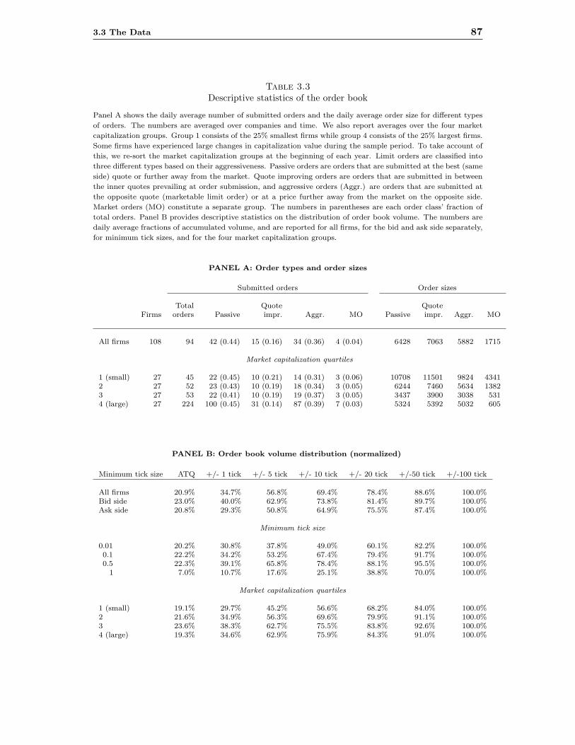
3.3 The Data 87
Table 3.3Descriptive statistics of the order book
Panel A shows the daily average number of submitted orders and the daily average order size for different types
of orders. The numbers are averaged over companies and time. We also report averages over the four market
capitalization groups. Group 1 consists of the 25% smallest firms while group 4 consists of the 25% largest firms.
Some firms have experienced large changes in capitalization value during the sample period. To take account of
this, we re-sort the market capitalization groups at the beginning of each year. Limit orders are classified into
three different types based on their aggressiveness. Passive orders are orders that are submitted at the best (same
side) quote or further away from the market. Quote improving orders are orders that are submitted in between
the inner quotes prevailing at order submission, and aggressive orders (Aggr.) are orders that are submitted at
the opposite quote (marketable limit order) or at a price further away from the market on the opposite side.
Market orders (MO) constitute a separate group. The numbers in parentheses are each order class’ fraction of
total orders. Panel B provides descriptive statistics on the distribution of order book volume. The numbers are
daily average fractions of accumulated volume, and are reported for all firms, for the bid and ask side separately,
for minimum tick sizes, and for the four market capitalization groups.
PANEL A: Order types and order sizes
Submitted orders Order sizes
Total Quote QuoteFirms orders Passive impr. Aggr. MO Passive impr. Aggr. MO
All firms 108 94 42 (0.44) 15 (0.16) 34 (0.36) 4 (0.04) 6428 7063 5882 1715
Market capitalization quartiles
1 (small) 27 45 22 (0.45) 10 (0.21) 14 (0.31) 3 (0.06) 10708 11501 9824 43412 27 52 23 (0.43) 10 (0.19) 18 (0.34) 3 (0.05) 6244 7460 5634 13823 27 53 22 (0.41) 10 (0.19) 19 (0.37) 3 (0.05) 3437 3900 3038 5314 (large) 27 224 100 (0.45) 31 (0.14) 87 (0.39) 7 (0.03) 5324 5392 5032 605
PANEL B: Order book volume distribution (normalized)
Minimum tick size ATQ +/- 1 tick +/- 5 tick +/- 10 tick +/- 20 tick +/-50 tick +/-100 tick
All firms 20.9% 34.7% 56.8% 69.4% 78.4% 88.6% 100.0%Bid side 23.0% 40.0% 62.9% 73.8% 81.4% 89.7% 100.0%Ask side 20.8% 29.3% 50.8% 64.9% 75.5% 87.4% 100.0%
Minimum tick size
0.01 20.2% 30.8% 37.8% 49.0% 60.1% 82.2% 100.0%0.1 22.2% 34.2% 53.2% 67.4% 79.4% 91.7% 100.0%0.5 22.3% 39.1% 65.8% 78.4% 88.1% 95.5% 100.0%
1 7.0% 10.7% 17.6% 25.1% 38.8% 70.0% 100.0%
Market capitalization quartiles
1 (small) 19.1% 29.7% 45.2% 56.6% 68.2% 84.0% 100.0%2 21.6% 34.9% 56.3% 69.6% 79.9% 91.1% 100.0%3 23.6% 38.3% 62.7% 75.5% 83.8% 92.6% 100.0%4 (large) 19.3% 34.6% 62.9% 75.9% 84.3% 91.0% 100.0%
88 Chapter 3 Order Book Characteristics and the Volume-Volatility Relation
book is averaged over the 6 order book snapshots.22 The table shows the order bookdistribution across minimum tick sizes and market capitalization quartiles.23 Around35 percent of the order book depth is concentrated at the quotes or plus/minus onetick from the quotes. This is quite stable both across tick sizes and across market capquartiles. However, when we separate the bid and ask sides, we find that the volume onthe bid side is more concentrated at the inner quotes than the volume on the ask side.This is in line with the findings in several other empirical papers, and is consistent withthe interpretation that the price impact is larger for buy orders than for sell orders.24
Note that the depth within +/- 5 ticks, which is what Biais et al. (1995) investigate,only includes 56 percent of the total order book depth in our sample. There does notseem to be large differences in order depth across market capitalization quartiles. Thelargest tick size category is special in that it only contains one, highly volatile and veryactively traded, company.25 One interesting thing to note about this firm is that asmuch as 30 percent of the order book depth lies between 50 and 100 ticks away fromthe quotes, even though it has been one of the most heavily traded companies at theexchange during our sample period.
3.4 Intraday analysis of the order book
In this section, we discuss how to measure the shape of the order book, and presentstatistics on the limit order book at an intraday level.
3.4.1 The shape of the order book
Figure 3.2 shows the average order books for two companies listed on the OSE. The or-der books are averaged over the five last trading days in May 2001, and are normalizedin the sense that they show the percentage of shares in all orders within an increas-ing/decreasing number of ticks away from the quotes (zero in the figure is the bestquote on each side of the market). The upper graph shows the average order book forNorsk Hydro (NHY) while the lower graph shows the average order book for Opticom(OPC). Both companies are among the most liquid on the exchange.26 Norsk Hydro
22For instance, on the ask side of the book for one company/snapshot, we divide the aggregate numberof shares at each tick by the total number of shares supplied (offered) at that time/snapshot. We dothis for each snapshot, and average across all snapshots on the particular date to obtain the averagefraction supplied on each tick for the security. Since we limit the order book to orders within +/- 100ticks from the bid/ask midpoint, the fraction of aggregate volume at +/- 100 ticks is 100%.
23If a firm trades across two minimum tick size regimes on the same day, we remove that companyfor that day from the sample. The results do not change if we include these observations.
24See Chan and Lakonishok (1993), Chan and Lakonishok (1995), and Kalay et al. (2003)25The company is Opticom (OPC).26During the period illustrated in the figure, both companies traded in prices around NOK 400-500
and had a tick size of NOK 0.5. For Norsk Hydro the calculated average order book is based on around2000 orders with a share volume of around 400 000 shares. For Opticom the similar calculations arebased on around 4000 orders with a share volume of around 200 000 shares.
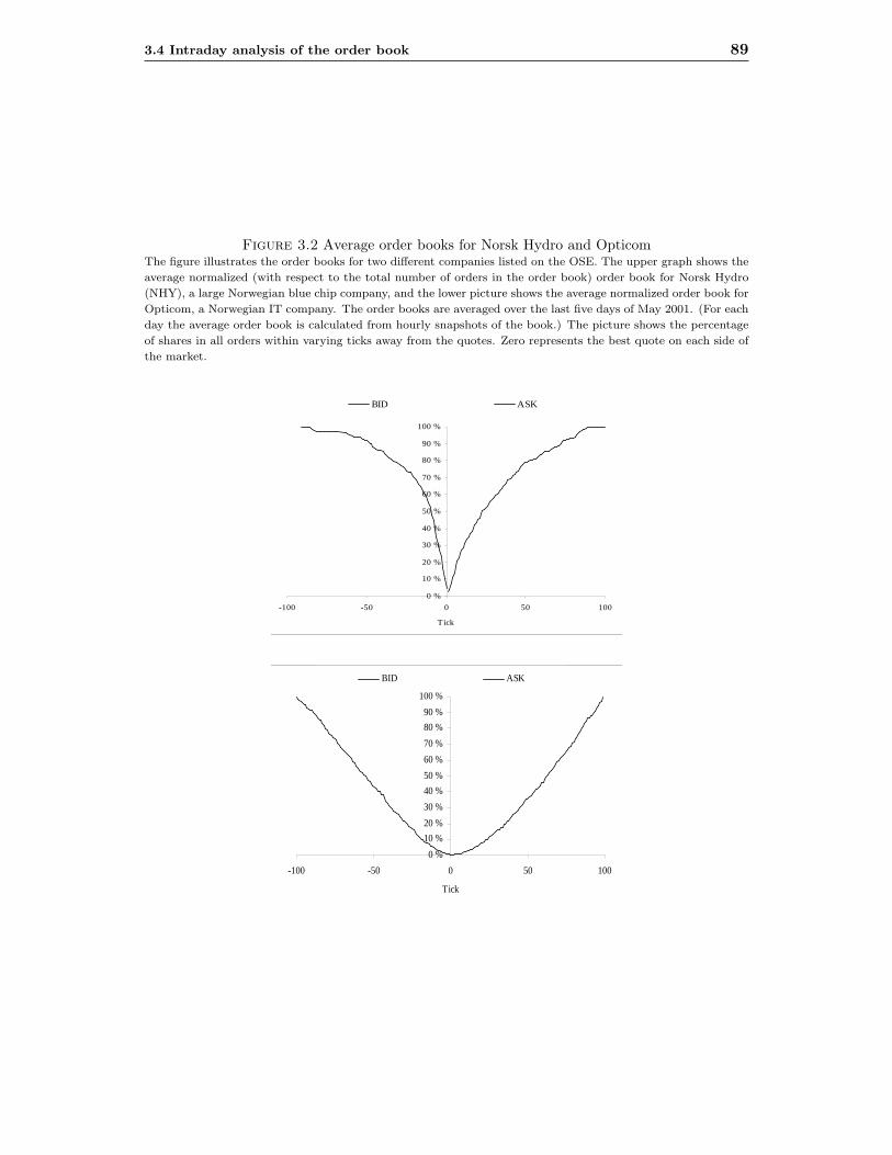
3.4 Intraday analysis of the order book 89
Figure 3.2 Average order books for Norsk Hydro and OpticomThe figure illustrates the order books for two different companies listed on the OSE. The upper graph shows the
average normalized (with respect to the total number of orders in the order book) order book for Norsk Hydro
(NHY), a large Norwegian blue chip company, and the lower picture shows the average normalized order book for
Opticom, a Norwegian IT company. The order books are averaged over the last five days of May 2001. (For each
day the average order book is calculated from hourly snapshots of the book.) The picture shows the percentage
of shares in all orders within varying ticks away from the quotes. Zero represents the best quote on each side of
the market.
0 %
10 %
20 %
30 %
40 %
50 %
60 %
70 %
80 %
90 %
100 %
-100 -50 0 50 100
Tick
BID ASK
0 %
10 %
20 %
30 %
40 %
50 %
60 %
70 %
80 %
90 %
100 %
-100 -50 0 50 100
Tick
BID ASK

90 Chapter 3 Order Book Characteristics and the Volume-Volatility Relation
is a leading energy, aluminium and fertilizer company, based in Norway. It has 50,000employees in 60 countries worldwide. The company’s operations are well known andthere is a a large amount of available information about the company, including experts’analysis. Opticom, on the other hand, is a relatively new IT company which currentlyhas under 100 employees. The company describes its business concept as pioneeringresearch and development in new technology in electronics. The company has no cashflow and very uncertain future income possibilities. Discussions in the popular presshave been largely focused on how difficult it is to value the company, and there havebeen large differences in analysts’ valuations. The picture shows that the order book ofthe two companies are quite different: while on average about 50 percent of the ordersfor Norsk Hydro has limit prices which lie within 5 ticks from the quoted spread, thesimilar percentage for Opticom is only about 10 percent.
This difference in the average shape of the order book results from the fact thattraders systematically submit orders further away from the midpoint in Opticom thanin Norsk Hydro. One possible reason for this is that investors are more uncertain aboutthe true value of Opticom than Norsk Hydro, and that this higher valuation uncertaintyin Opticom is reflected in orders being submitted across a wider range of prices thanin Norsk Hydro. The difference in the order book shapes may also come from pick-offrisk, i.e. the reservation prices reflect a compensation for the risk of being picked off bybetter informed traders. Probably both effects contribute to explaining the pictures wesee in figure 3.2. However, while it is obvious that there are huge differences in valuationuncertainty between the two companies, it is not so obvious that there should be such abig difference in pick-off risk. More importantly, pick-off risk should mainly concern theorders submitted close to the midpoint price. Thus, pick-off risk should affect the spreadand volumes at the inner ticks, not the distribution of orders across the the entire orderbook. The figure also illustrates the difference in order book liquidity between the bidand the ask side, which we documented for the whole sample in panel B in table 3.3.Although it is more pronounced for Norsk Hydro, both pictures indicate that the askside of the book is more elastic than the bid side.
Measuring the order book slope To capture the shape of the order book, we usethe average elasticity/slopes of the supply and demand schedules in the order book.The more gentle (steeper) the slope, the more widely distributed (concentrated) are thebid and ask prices in the order book. Note that we use the inverse of the elasticity, withprices on the x-axis and accumulated volumes on the y-axis, as in Biais et al. (1995).
To obtain an average slope of the order book, we divide the trading day into hourlyspaced intervals. At the end of each interval, we take a snapshot of the order book.These snapshots occur at 10:30, 11:30, 12:30, 13:30, 14:30 and 15:30 each trading dayfor each firm. Note that the first snapshot is half an hour after the regular trading

3.4 Intraday analysis of the order book 91
session starts. Alternatively, we could end the last snapshot at 16:00, but then theorder book would be affected by the large amount of order cancellations at the end ofthe trading day. To rebuild the order book we start at the beginning of the trading daywith the orders still remaining after the opening auction has been executed at 10:00.Then we track all types of orders being submitted throughout the day, and update theorder book accordingly. Thus, all deletions and/or amendments of earlier orders aswell as new orders are accounted for when we update the order book.27 After havingobtained the full order book for each snapshot we calculate our slope/elasticity estimatefor each company of the order book in the following steps:
1. First, for each side of the order book, and each snapshot, we accumulate theaggregate number of shares supplied/demanded at each price level, such that ateach price level we get the total volume supplied (demanded) at that price or lower(higher).
2. To account for large differences in liquidity between firms, we normalize the ac-cumulated shares at each tick level (on the ask and bid side separately) relativeto the total number of shares supplied/demanded at the relevant snapshot. Thus,the percentage of the shares in the order book supplied (demanded) at the highest(lowest) ask (bid) price/tick is 100 percent.
3. Next, we calculate the “local” elasticity at each price level (illustrated in equa-tion 3A.2 and equation 3A.3 in the appendix).
4. Then, we average across all price levels (local slopes) to obtain an average elastic-ity/slope for the bid and ask side for that snapshot.
5. Finally, we take the average of the bid and ask slope to get one slope measurefor the snapshot and average across all the snapshots during the trading day toobtain the average slope for each company on that day.
We normalize the order book because we want to take into account that there is a closerelationship between our slope measure and the liquidity of the underlying stock. Lessliquid firms generally have a higher volatility since the order book does not containenough volume to absorb large trades without moving prices too much. In addition,less liquid stocks generally have a higher spread since investors require a discount whenbuying and a premium when selling the stock. Thus, a positive relationship betweenorder book elasticity and volatility is expected a priori. By normalizing the order book,we get the fraction of total shares supplied/demanded at each price level regardless of
27The original dataset from the Oslo Stock Exchange includes order book data for the best 5 quoteson each side whenever a new order is submitted or there is a deletion or amendment of an existing order.We use this information to check that our order book is correct for these 5 levels of the book.

92 Chapter 3 Order Book Characteristics and the Volume-Volatility Relation
the total volume in the order book. This makes the order books more comparable acrossfirms and time.
In addition to the equally weighted slope of the order book (across tick levels), wecalculate a slope measure where we weight each local slope by its distance (in ticks)from the inner quote. The tick-weighting implies that local slopes further out in thebook have a lower impact on the average slope than local slopes closer to the midpointprice. The main reason for doing this is to reduce the effects that “stale” orders mayhave on the “tails” of the order book.
Figure 3.3 illustrates how the local elasticities, ∆Aτ and ∆B
τ , are calculated. Forillustrative purposes, the order book in the figure stretches only across 4 price levels oneach side. In the figure, pA
1 is the best available ask price (inner ask quote) with volumefraction of vA
1 supplied at that ask price. The volume fraction at the next tick level(vA
2 ) is thus the accumulated volume supplied at price pA1 and pA
2 relative to the totalvolume in the order book on each side. The local elasticity of the supply curve at pA
1
would thus be the slope ∆A2 in the figure. A more specific explanation of the calculation
is provided in the appendix.When we normalize the order book, the slope measures the average percentage
change in normalized volume when the price level changes by one percent. For example,suppose that the current bid price is 49 (ask price is 50), the normalized depth is 10percent and the slope is 10. If the bid-price decreases by 1 percent to 48.5 (or the askprice increases by 1 percent to 50.5), the normalized depth will increase by 10 percentto 11 percent.
3.4.2 Intraday Statistics
Table 3.4 shows intraday statistics for our slope measure (calculated at the end of eachtime interval), the price volatility (measured as the absolute hourly return betweenmidpoint prices closest to the end of each time interval), the quoted and the effectivespread, the number of trades executed during the time interval, the trade and ordersizes measured in shares, and the number of orders submitted during the time interval.All numbers are daily averages across all firms in the sample, and the time intervalscorrespond to those used for rebuilding the order book.
Notable characteristics of the intraday statistics in table 3.4 are;
• The average slope increases at a decreasing rate throughout the day.
• The quoted and the effective spread both have a U-shape, with the highest spreadat the beginning of the day.
• The average trade size is smallest at the beginning of the day, and increasingthroughout the trading day.

3.4 Intraday analysis of the order book 93
Figure 3.3 Calculation of the demand and supply elasticitiesThe figure illustrates how the local slopes/elasticities on the bid and ask side of the order book are calculated
for one ”snapshot” time on one date for one company. There are only 4 price levels on both sides of the book.
The left y-axis shows the fraction of aggregate share volume on the demand (bid) side of the order book at each
tick level. Similarly, the right y-axis shows the fraction of aggregate share volume on the supply (ask) side of the
order book at each tick level. The solid step-line is the supply (right) and demand (left) curves over the various
price levels. On the x-axis, we have the various price levels. pM is the bid/ask midpoint. Prices greater than
pM are ask prices and prices below pM are bid prices. The difference between pB1 (best bid) and pA
1 (best ask)
is the quoted spread. The dotted line-segments connecting each level of the order book have local slopes denoted
by ∆s. These are the normalized local elasticities of the demand and supply curves calculated in equation 3A.2
and equation 3A.3 in the appendix.
�
Y1
Fraction ofbid volume Fraction of
ask volume
Price attick level
�
1∆
�
2∆
�
3∆
�
4∆
�
1∆
�
2∆
�
3∆
�
4∆
�
S1
S2
S3
S4
�
S4
�
S3
S2
�
S1
�
Y2
�
Y3
14 =�
Y
�
Y1
�
Y2
�
Y3
14 =�
Y
�
S
Table 3.4Intraday statistics
The table provides intraday statistics for the data sample, including the slope measure, the volatility (the absolute
hourly return between trade prices closest to the end of each interval), the quoted spread, the effective spread,
the number of trades executed during the time interval, the trade size (in shares), the number of orders submitted
during the time interval, and the order size (in shares). All numbers are daily averages across all firms in the
sample. Note that the first and last time windows are half an hour while the rest of the time windows are hourly.
The slope is calculated at the end of each interval.
Time window10:00 to 10:30 to 11:30 to 12:30 to 13:30 to 14:30 to 15:30 to
10:30 11:30 12:30 13:30 14:30 15:30 16:00
Slope (end of time window) 30.51 34.37 35.78 36.34 36.80 36.97 -Volatility (absolute return) - 1.34% 0.81% 0.72% 0.74% 0.88% 0.86%Quoted spread 2.36 1.73 1.47 1.37 1.33 1.31 1.39Effective spread 1.79 1.27 1.05 1.00 0.95 0.95 1.05
Trades 10.38 11.81 9.38 9.05 9.52 10.81 10.40Trade size (shares) 2314 2653 2759 2774 2834 3027 3123Orders 15.45 18.16 13.10 12.36 12.47 14.02 11.66Order size (shares) 6858 6385 5723 5818 5795 6383 6706

94 Chapter 3 Order Book Characteristics and the Volume-Volatility Relation
• The average number of orders and trades both follow a U-shape, with fewer ordersbeing placed and trades being executed in the middle of the day, and most ordersbeing placed and trades being executed at the beginning of the day.
These regularities are also systematic across sub-periods.28 Similar systematic intradayregularities have been found in other markets (e.g. US, France, Hong Kong, Sweden).29
Following the sequential trading model in Glosten and Milgrom (1985), these datafeatures can be explained by higher uncertainty about other traders’ valuations at thebeginning of the trading day than during the day. If this explanation is correct, a patientliquidity trader who fears being picked off by informed investors at the beginning of theday has two main options. If she believes that the probability of trading with informedtraders will diminish during the day, she can act strategically and delay her trading.Alternatively, she can submit her orders at the beginning of the day and take accountof the increased probability of incurring a loss by placing them at prices includinga discount (buys) or a premium (sells). This can explain the higher spread at thebeginning of the trading day. The increase in spreads towards the end of the day maybe due to higher liquidity demand and possibly more cancellation of orders just beforethe close. Assuming that the informed traders are trying not to reveal their informationtoo quickly, we would also expect to see a higher number of small trades at the beginningof the trading day (stealth trading).
To obtain a measure of order aggressiveness during the trading day, we calculate aseparate index similar to Harris and Hasbrouck (1996), where the aggressiveness of anorder is measured by the average number of ticks the order is placed away from the bestquote (on the same side). Thus an index number of zero means that the average orderis placed at the quote, a positive index number means that the order is placed above(below) the bid (ask), and a negative number means that the average order is placedbelow (above) the bid (ask).30 Formally, for an order of type k, the aggressiveness of abuy order with a limit price pB is calculated as,
λbuyk = (pB − bid)/ticksize (3.2)
Similarly, a sell order with a limit price pS is calculated as,
λsellk = (ask − pS)/ticksize (3.3)
where bid and ask are the best bid quote and best ask quote, respectively, when the28We also calculate the statistics across sub-periods of years, half-years and quarters and find that
the results are both qualitatively and quantitatively similar.29For the US, see French and Roll (1986) and Harris (1986). For Sweden, see Niemeyer and Sandas
(1995).30We cannot calculate the aggressiveness for market orders since these orders do not have a price
limit.
3.4 Intraday analysis of the order book 95
order is submitted.Table 3.5 shows the intraday pattern in order aggressiveness, average number of
orders, fraction of order types, and order sizes. Figure 3.4 illustrates graphically theintraday patterns in order aggressiveness, order size, order book slope, quoted andeffective spread, and fraction of order types.
If uninformed investors believe that there is more asymmetric information at thebeginning of the trading day, we would expect to see that they place orders at limit pricesfurther away from the midpoint price at the beginning of the trading day, and then,closer to the midpoint prices later in the day, as the market price adjusts to reflect theprivate information. This is consistent with a Glosten and Milgrom (1985) type of modelwhere trading is sequential and uncertainty is greatest at the opening of the tradingsession. Moreover, we would expect that the orders placed by better informed investorswere most aggressive at the beginning of the day, especially if informed investors arecompeting to extract profits from the same information. This is exactly what is indicatedin our data sample. Table 3.4 and figure 3.4 show that there are systematic differencesin the aggressiveness of different types of orders in the course of the trading day.
“Away from market” orders, which make up a large part of the order book, areplaced further away from the inner quotes at the beginning than at the end of the day.If this type of order is mainly submitted by uninformed traders, it indicates that theyrequire a higher compensation for trading early in the day relative to later in the day.Another interpretation is that uninformed traders have not yet processed all publiclyavailable information (e.g. newspapers, new analyzes, gossip etc.), and are more pas-sive when submitting their orders before they have been able to read and interpret thisinformation. Orders that are more aggressive, and likely to stem from better informedinvestors or pre-committed liquidity traders, are relatively more aggressive at the be-ginning of the day than later in the day. Thus, a pre-committed trader or informedtrader, demanding liquidity, needs to be relatively more aggressive at the beginning ofthe day to get his order executed since the liquidity suppliers submit their orders rel-atively much further away from the midpoint. At the end of the trading day all typesof orders are submitted closer to the inner quotes, indicating that the adverse selectioncost is reduced. Assuming that all other cost components of the spread, except theadverse selection component, are fixed through the day, the decrease in spreads mayalso reflect that the adverse selection cost is the largest at the beginning of the day andsmaller at the end of the day.
The average number of passive orders (“away from market”) and market ordersdecreases throughout the day, while the average number of quote-improving orders andaggressive orders has a U-shape. The intraday pattern in the relative fraction of eachorder type indicates that more orders are submitted closer to the midpoint at the endof the day. “Away from the market” orders are the largest at the open and close, while
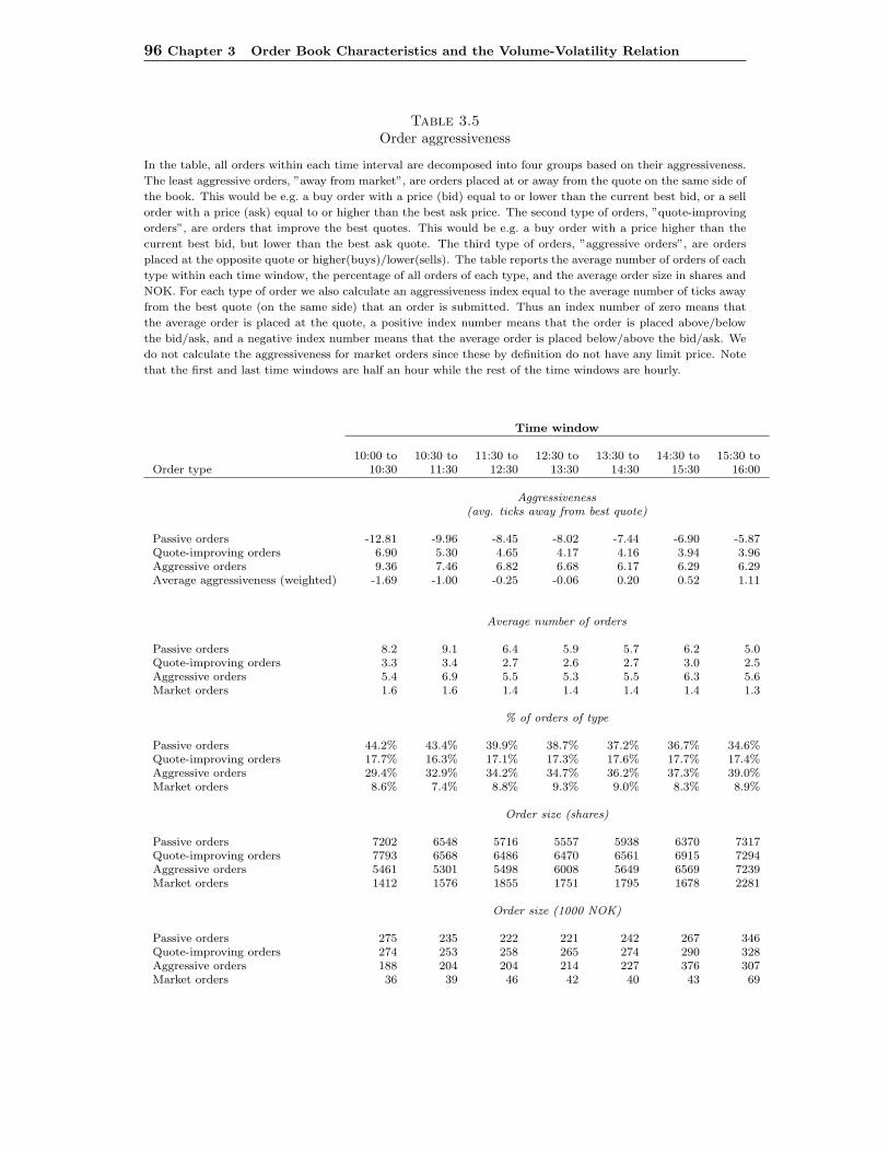
96 Chapter 3 Order Book Characteristics and the Volume-Volatility Relation
Table 3.5Order aggressiveness
In the table, all orders within each time interval are decomposed into four groups based on their aggressiveness.
The least aggressive orders, ”away from market”, are orders placed at or away from the quote on the same side of
the book. This would be e.g. a buy order with a price (bid) equal to or lower than the current best bid, or a sell
order with a price (ask) equal to or higher than the best ask price. The second type of orders, ”quote-improving
orders”, are orders that improve the best quotes. This would be e.g. a buy order with a price higher than the
current best bid, but lower than the best ask quote. The third type of orders, ”aggressive orders”, are orders
placed at the opposite quote or higher(buys)/lower(sells). The table reports the average number of orders of each
type within each time window, the percentage of all orders of each type, and the average order size in shares and
NOK. For each type of order we also calculate an aggressiveness index equal to the average number of ticks away
from the best quote (on the same side) that an order is submitted. Thus an index number of zero means that
the average order is placed at the quote, a positive index number means that the order is placed above/below
the bid/ask, and a negative index number means that the average order is placed below/above the bid/ask. We
do not calculate the aggressiveness for market orders since these by definition do not have any limit price. Note
that the first and last time windows are half an hour while the rest of the time windows are hourly.
Time window
10:00 to 10:30 to 11:30 to 12:30 to 13:30 to 14:30 to 15:30 toOrder type 10:30 11:30 12:30 13:30 14:30 15:30 16:00
Aggressiveness(avg. ticks away from best quote)
Passive orders -12.81 -9.96 -8.45 -8.02 -7.44 -6.90 -5.87Quote-improving orders 6.90 5.30 4.65 4.17 4.16 3.94 3.96Aggressive orders 9.36 7.46 6.82 6.68 6.17 6.29 6.29Average aggressiveness (weighted) -1.69 -1.00 -0.25 -0.06 0.20 0.52 1.11
Average number of orders
Passive orders 8.2 9.1 6.4 5.9 5.7 6.2 5.0Quote-improving orders 3.3 3.4 2.7 2.6 2.7 3.0 2.5Aggressive orders 5.4 6.9 5.5 5.3 5.5 6.3 5.6Market orders 1.6 1.6 1.4 1.4 1.4 1.4 1.3
% of orders of type
Passive orders 44.2% 43.4% 39.9% 38.7% 37.2% 36.7% 34.6%Quote-improving orders 17.7% 16.3% 17.1% 17.3% 17.6% 17.7% 17.4%Aggressive orders 29.4% 32.9% 34.2% 34.7% 36.2% 37.3% 39.0%Market orders 8.6% 7.4% 8.8% 9.3% 9.0% 8.3% 8.9%
Order size (shares)
Passive orders 7202 6548 5716 5557 5938 6370 7317Quote-improving orders 7793 6568 6486 6470 6561 6915 7294Aggressive orders 5461 5301 5498 6008 5649 6569 7239Market orders 1412 1576 1855 1751 1795 1678 2281
Order size (1000 NOK)
Passive orders 275 235 222 221 242 267 346Quote-improving orders 274 253 258 265 274 290 328Aggressive orders 188 204 204 214 227 376 307Market orders 36 39 46 42 40 43 69
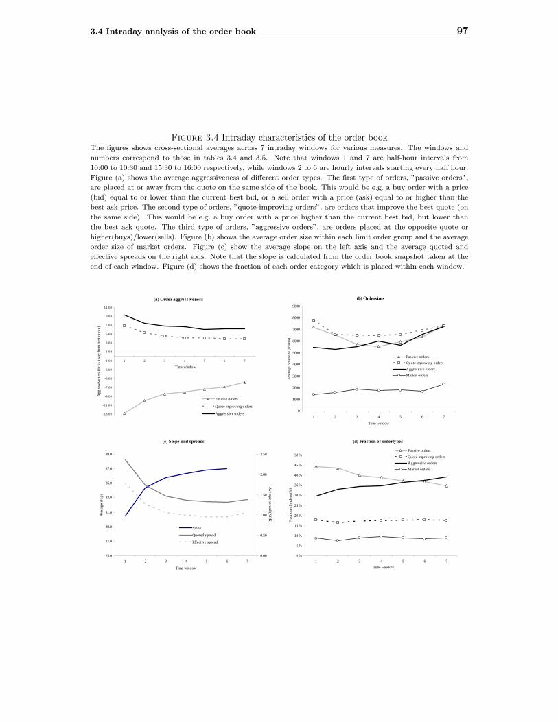
3.4 Intraday analysis of the order book 97
Figure 3.4 Intraday characteristics of the order bookThe figures shows cross-sectional averages across 7 intraday windows for various measures. The windows and
numbers correspond to those in tables 3.4 and 3.5. Note that windows 1 and 7 are half-hour intervals from
10:00 to 10:30 and 15:30 to 16:00 respectively, while windows 2 to 6 are hourly intervals starting every half hour.
Figure (a) shows the average aggressiveness of different order types. The first type of orders, ”passive orders”,
are placed at or away from the quote on the same side of the book. This would be e.g. a buy order with a price
(bid) equal to or lower than the current best bid, or a sell order with a price (ask) equal to or higher than the
best ask price. The second type of orders, ”quote-improving orders”, are orders that improve the best quote (on
the same side). This would be e.g. a buy order with a price higher than the current best bid, but lower than
the best ask quote. The third type of orders, ”aggressive orders”, are orders placed at the opposite quote or
higher(buys)/lower(sells). Figure (b) shows the average order size within each limit order group and the average
order size of market orders. Figure (c) show the average slope on the left axis and the average quoted and
effective spreads on the right axis. Note that the slope is calculated from the order book snapshot taken at the
end of each window. Figure (d) shows the fraction of each order category which is placed within each window.
�D��2UGHU�DJJUHVVLYHQHVV
-13.00
-11.00
-9.00
-7.00
-5.00
-3.00
-1.00
1.00
3.00
5.00
7.00
9.00
11.00
1 2 3 4 5 6 7
Time window
Agg
ress
iven
ess
(tic
ks a
way
from
bes
t quo
te)
Passive orders
Quote improving orders
Aggressive orders
�F��6ORSH�DQG�VSUHDGV
25.0
27.0
29.0
31.0
33.0
35.0
37.0
39.0
1 2 3 4 5 6 7
Time window
Ave
rage
slo
pe
0.00
0.50
1.00
1.50
2.00
2.50
Average spread (N
OK
)
Slope
Quoted spread
Effective spread
�E��2UGHUVL]HV
0
1000
2000
3000
4000
5000
6000
7000
8000
9000
1 2 3 4 5 6 7
Time window
Ave
rage
ord
ersi
ze (s
hare
s)
Passive orders
Quote improving orders
Aggressive orders
Market orders
�G��)UDFWLRQ�RI�RUGHUW\SHV
0 %
5 %
10 %
15 %
20 %
25 %
30 %
35 %
40 %
45 %
50 %
1 2 3 4 5 6 7
Time window
Frac
tion
of o
rder
s (%
)
Passive orders
Quote improving orders
Aggressive orders
Market orders

98 Chapter 3 Order Book Characteristics and the Volume-Volatility Relation
the most aggressive limit orders and market orders are the smallest and increase in sizethroughout the day. If informed investors mainly use aggressive limit orders and marketorders, this may indicate that they submit smaller orders when their information is themost valuable (stealth trading).
The evidence that there is more asymmetric information at the beginning of thetrading day is also captured by the intraday pattern of our slope estimate. The slopeincreases (at a diminishing rate) across the day, with a minimum at the beginning ofthe day and a maximum at the end of the day, which indicates that the order book ismore dispersed in the morning relative to later in the day. Note that the average slopeis calculated from the normalized order book, i.e. the slope does not merely reflect thatthere are fewer orders in the order book early in the day, but rather that orders aresubmitted across a wider price range.31 Over time windows, the average slope increasesat a diminishing rate as the order book becomes more concentrated and inelastic at theend of the day.
3.5 The Volume-Volatility Relation
In this section, we first document that there exist a volume-volatility relation in theNorwegian equity market as has been found for the US by e.g. Jones et al. (1994) andin the UK by Huang and Masulis (2003). When we decompose volume into trades andorder size, and interpret the number of trades as a proxy for the mixing variable, we findsupport for the MDH. We then investigate the relationship between volume, volatilityand the slope of the order book.
3.5.1 The Volume-Volatility Relation in a Limit Order Market
To investigate if there is a volume-volatility relation in our data sample, we follow theregression approach in Jones et al. (1994). First, we measure the daily return volatilityusing the standard procedure in similar empirical studies,32 by running the followingregression for each firm i,
Ri,t =
5∑k=1
αi,kDk,t +
12∑j=1
βi,jRi,t−j + εi,t (3.4)
where Ri,t is the return of security i on day t, and Dk,t is a day-of-the-week dummy forday k. To avoid measurement errors due to the bid-ask bounce, we calculate returnsfrom the average of bid-ask prices at the close. The 12 lagged return regressors esti-mate short-term movements in conditional expected returns. The residual, εi,t, is our
31A lower average slope reflects that the order book is more elastic, which implies that a lower fractionof the order volume is close to the inner quotes relative to further out in the book.
32See Schwert (1990), Bessembinder and Seguin (1993), Jones et al. (1994), and Daigler and Wiley(1999).

3.5 The Volume-Volatility Relation 99
estimate of the unexpected return of security i on date t. The absolute value of thismeasure constitute our measure of volatility. Next, we estimate the regression equationssuggested in Jones et al. (1994) to determine the relative effects of number of trades(N) and trade-size (AV) for volatility,
Model I: |εt,i| = αi + αi,mMt + βiAVi,t +
12∑j=1
ρi,j|εi,t−j| + ηi,t (3.5)
Model II: |εt,i| = αi + αi,mMt + γiNi,t +
12∑j=1
ρi,j|εi,t−j| + ηi,t (3.6)
Model III: |εt,i| = αi + αi,mMt + βiAVi,t + γiNi, t +
12∑j=1
ρi,j|εi,t−j| + ηi,t (3.7)
The ρi,j’s measure the persistence in volatility across 12 lags. Mt is a dummy variablethat is equal to 1 for Mondays and 0 otherwise, AVi,t is the average trade size (totalnumber of shares traded divided by the number of transactions for stock i on date t),and Ni,t is the number of transactions in security i on date t. The regressions are runfor each firm and then the parameter estimates are averaged across firms.
The first part of table 3.6 provides the results from the estimation of regressionequations 3.5-3.7 using daily returns for all companies in our filtered sample. Overall,our results are very much in line with the results in Jones et al. (1994). The explanatorypower of model 2 (with respect to the adjusted R-squared), where volume is measuredby the average number of daily trades, is almost the double of the explanatory powerof model 1, where volume is measured by the average trade size. Moreover, the averagetrade size has little marginal explanatory power when volatility is conditioned on thenumber of transactions in model 3. These results are further supported by the char-acteristics of the sampling distributions of individual-firm coefficients and t-statisticsof the two variables. In model 3, 95.4 percent of the coefficients for the average num-ber of trades are statistically significant, and 99.1 percent of the average number oftrades coefficients were greater than zero. Similar numbers for the average trade sizeare respectively 24.1 percent and 57.4 percent.
As a robustness check we also estimate the equations for sub-periods of half-years.Although not reported in a table, the results from the whole sample regression areconfirmed in the sub-sample regressions. Most notably, the γ estimates of the effect oftrades (N), as well as their distributional properties, are very stable across sub-periods.The β estimates, however, vary considerably across sub-periods and are less significantthan γ for model 1 relative to model 3.
Jones et al. (1994) find that trade size has some information content for some ofthe smaller Nasdaq-NMS firms. This finding is interpreted as supportive of the notionthat private information based trading is important only for the smallest firms on the
100 Chapter 3 Order Book Characteristics and the Volume-Volatility Relation
stock market. To check for similar features in our data sample, we re-estimate thethree regression models on the four size portfolios. The results from these estimationsare presented in the second part of table 3.6. In general, the results from estimatingseparate regression models for each size portfolio are similar to the results from runningone regression for the whole sample. However, we find the opposite result from Joneset al. (1994) that the explanatory power of trade size is the strongest for the largestfirms. On the other hand, only about half of the parameter estimates for trade size inthe single firm regressions are greater than zero, indicating that the effect may not bevery systematic across firms.
3.5.2 Volume, volatility and the limit order book
We now turn to the question whether the slope of the order book affect volatility andtrading activity. The reported results are based on the equally weighted slope calcu-lated from the normalized order book. As discussed in section 3.4 and appendix 3.A,we also calculate a tick-weighted slope measure. The two slope measures are highlycorrelated (0.98), and the results from using the weighted slope measure are quite sim-ilar to those obtained using the equally weighted measure.33 The correlations betweenthe equally weighted slope and the other variables used in our analysis are reported intable 3.7. Table 3.8 provides some descriptive statistics on the distribution of the dailyslope estimate over the whole sample, for the separate years, and for the four marketcapitalization groups.
Table 3.7 shows that the slope measure has the expected close relationship to mea-sures of liquidity such as market capitalization (positive correlation of 0.44) and quotedpercentage spread (negative correlation of -0.32). Thus, larger firms are generally moreliquid, with a smaller spread and a steeper slope. One reason for this may be thatlarger firms generally are easier to value, making the dispersion of prices in the orderbook more concentrated around the midpoint price. In addition, we see that there isa positive correlation of 0.13 between the slope and the number of trades. Further,table 3.8 shows that larger and more liquid stocks have a higher fraction of the orderbook volume concentrated at or around the best quotes, while smaller firms have moreelastic order books. This is also evident from panel B in table 3.3.
Figure 3.5 illustrates the relationship between the daily slope and the contempora-neous daily price changes at an aggregate level. Daily price changes are measured as theaverage daily absolute return over the trading day.34 Both variables are daily equallyweighted averages across all traded securities. Interestingly, even at this aggregate levelthe figure indicates that the price volatility is higher (lower) when the average dailyslope of the order book is low (high). Another notable feature is that the average slope
33Estimation results for when we use the weighted slope version are reported in appendix 3.C.34cf equation 3.4.

3.5 The Volume-Volatility Relation 101
Table 3.6A volume-volatility regression model
The table reports the results from the estimation of three regression models of the volume/trade size -volatility
relation. The models are estimated on the whole data sample and separately for each market capitalization
group. The models are based on Jones et al. (1994):
Model I: |εt,i| = αi + αi,mMt + βiAVi,t +
12∑j=1
ρi,j|εi,t−j| + ηi,t
Model II: |εt,i| = αi + αi,mMt + γiNi,t +
12∑j=1
ρi,j|εi,t−j| + ηi,t
Model III: |εt,i| = αi + αi,mMt + βiAVi,t + γiNi, t +
12∑j=1
ρi,j|εi,t−j| + ηi,t
Using the Jones et al. (1994) notation we have that |εt,i| is the absolute value of the return of security i in
period t, conditional on its own 12 lags and day-of-week dummies, Mt is a dummy variable that is equal to 1
for Mondays and 0 otherwise, AVi,t is the average trade size, Ni,t is the number of transactions for security i
on day t, and the coefficients ρi,t measure the persistence in volatility. Column 3-5 show parameter estimates
averaged across all individual firm regression equations, while columns 6-9 show the parameter distribution across
firms. β is the average parameter estimate for the average trade size variable (AV), γ is the average parameter
estimate for the number of trades variable (N). In the distribution of estimates column we report, respectively,
the percentage of β and γ estimates over all single firm regression equations that are significant. In the last two
columns we report the percentage of parameter estimates that are greater than zero. The first part of the table
shows the results from running the regression equations over the whole sample. The second part of the table
shows the similar results when we split the sample into four size portfolios.
Parameter estimates Distribution of estimates
Model Firms β (AV) γ (N) adj. R2 %t(β)>2 %t(γ)>2 %β>0 %γ>0
Model I (AV) 108 0.145 - 0.057 26.9% - 81.5% -Model II (N) 108 - 0.031 0.145 - 95.4% - 100.0%Model III (AV,N) 108 0.053 0.031 0.149 22.2% 94.4% 58.3% 100.0%
Model I (AV)1 (small) 27 0.145 - 0.080 16.2% - 78.4% -2 27 0.219 - 0.055 18.2% - 77.3% -3 27 0.274 - 0.048 19.0% - 64.3% -4 (large) 27 1.021 - 0.038 30.8% - 79.5% -
Model II (N)1 (small) 27 - 0.052 0.174 - 89.2% - 97.3%2 27 - 0.028 0.147 - 75.0% - 95.5%3 27 - 0.036 0.136 - 81.0% - 95.2%4 (large) 27 - 0.014 0.174 - 79.5% - 92.3%
Model III (AV,N)1 (small) 27 0.079 0.053 0.175 10.8% 86.5% 64.9% 97.3%2 27 0.076 0.030 0.148 4.5% 75.0% 54.5% 95.5%3 27 0.075 0.036 0.140 16.7% 78.6% 45.2% 95.2%4 (large) 27 0.237 0.014 0.179 30.8% 82.1% 35.9% 94.9%

102 Chapter 3 Order Book Characteristics and the Volume-Volatility Relation
Table 3.7Variable correlations
The table shows Pearsons’ correlation coefficients between our elasticity variable (SLOPE) and various trading
activity and liquidity variables.
Trade size OrderTrades (N) shares (AV) MCAP SPREAD SLOPE volume (OV)
Trade size shares (AV) -0.02MCAP 0.25 -0.04SPREAD -0.20 0.16 -0.17SLOPE 0.13 -0.08 0.44 -0.32Order volume shares (OV) 0.19 0.16 0.06 -0.06 0.04Trade volume shares (V) 0.43 0.33 0.14 -0.13 0.08 0.45
is steeper in the first half of the sample, with an average slope of about 41, than duringthe second part of the sample when the average slope drops to about 35. These twoperiods coincide quite well with the boom and burst of the internet bubble. It is notobvious that increased trading activity due to arrival of new information can explainthe volatility pattern during this period. If the slope proxies for valuation uncertainty,the pattern in the figure reflects greater agreement among traders about asset valuesduring the build-up of the bubble than during the subsequent market down-turn.
3.5.3 Daily volatility and order book shape
To examine whether our slope measure can explain the contemporaneous volatilityacross firms and time, we estimate modified versions of the volume-volatility regres-sion equations in section 3.5.1. More specifically, we estimate 3 different versions of thefollowing cross-sectional time-series regression model with one-way fixed effects,
| εit |=
K∑k=1
Xitkβk + ηi,t (3.8)
where | εit | is the daily volatility estimate from equation 3.4, Xitk is the matrix ofexplanatory variables (k) across time (t) for each company (i) and ηi,t = νi + εi,t
defines the error structure with νi as the non-random fixed, firm-specific, effect. Sincewe use one-way fixed effects specification, the estimation is analogous to a least-squaresdummy variable (LSDV) regression with firm-specific constants νi. Since not all firmsare traded every day, our sample is unbalanced35. However, results from estimating thesame models on a balanced sample are quantitatively similar.36
35We use the TSCSREG procedure supplied with SAS v.8.2 for estimating the models. The procedureis capable of processing data with different numbers of time-series observations across different crosssections.
36In the unbalanced sample, all firms with 400 trading days or more throughout the sample period of597 days are included. In the balanced sample, we filter out all firms which are not traded every dayduring the sample period. This filter reduces the sample to 25 firms. See appendix 3.B for estimation

3.5 The Volume-Volatility Relation 103
Table 3.8Distribution of slope estimates
The table shows the distribution of the slope estimates where each local slope is equally weighted, and each
side of the order book is normalized with respect to the total number of shares on each side. Panel A report
the estimates for the entire sample and across minimum tick sizes. Panel B report the estimates across market
capitalization groups and years. Each company is assigned to a market capitalization quartile at the end of every
trading day. N reflects the number of firm/date observations, MCAP is the average market capitalization in
NOK millions, price is the average price, P5, P10, P25, P75, P90, and P95 are the 5th, 10th 25th 75th, 90th and
95th percentiles respectively.
PANEL A
Distribution of daily SLOPE estimatesN MCAP Price P5 P10 P25 Median Mean P75 P90 P95
All firms 51015 7294 145 9.1 11.9 18.3 29.2 37.2 46.7 70.9 91.51999 16968 5948 110 9.4 12.6 20.3 33.2 41.4 53.0 79.2 101.32000 23853 7737 180 9.6 12.2 18.0 27.6 35.3 43.5 66.3 86.02001 10194 8498 122 7.8 10.6 16.5 27.0 34.7 43.4 65.2 85.7
PANEL B
Distribution of daily SLOPE estimatesN MCAP Price P5 P10 P25 Median Mean P75 P90 P95
MCAP Q1 (small) 12532 259 21 5.7 7.4 11.4 17.2 20.9 25.9 38.2 47.91999 4163 213 19 5.9 7.5 11.4 17.5 21.2 26.7 39.3 48.22000 5864 282 22 6.3 8.2 12.1 17.6 20.9 25.7 36.6 45.92001 2505 283 22 4.6 6.0 10.0 15.9 20.5 25.2 40.4 50.9
MCAP Q2 12828 1005 64 10.6 12.9 18.1 26.3 31.8 39.0 56.4 70.91999 4264 869 50 11.3 14.0 19.7 28.8 34.0 41.8 59.3 74.42000 5999 1035 69 10.7 12.8 17.7 25.1 30.2 36.9 53.1 66.82001 2565 1158 76 9.8 12.0 16.9 25.2 31.8 39.2 57.8 73.2
MCAP Q3 12672 2786 121 12.0 15.3 22.2 32.5 39.0 48.1 69.9 87.21999 4210 2289 106 15.3 19.1 26.5 38.1 45.2 55.8 78.9 98.12000 5934 2914 133 11.6 14.7 21.1 30.4 36.5 44.3 65.0 82.42001 2528 3315 121 10.6 13.1 19.5 28.9 34.5 43.0 61.3 75.8
MCAP Q4 (large) 12983 24698 369 18.0 22.1 31.6 47.1 56.5 69.4 101.6 128.81999 4331 20016 261 23.0 28.2 38.9 55.7 64.2 79.0 111.6 136.62000 6056 26320 491 16.7 21.0 29.2 44.0 53.1 64.6 94.6 120.32001 2596 28727 263 15.7 19.9 27.8 41.1 51.5 61.5 96.6 125.9
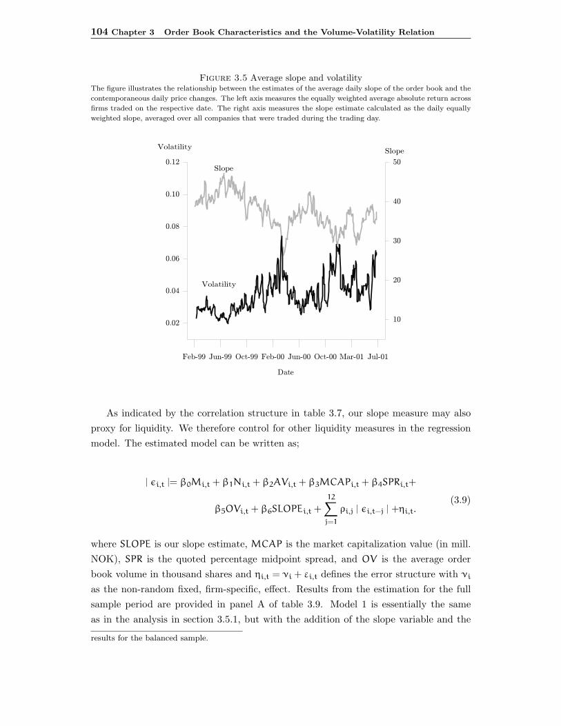
104 Chapter 3 Order Book Characteristics and the Volume-Volatility Relation
Figure 3.5 Average slope and volatilityThe figure illustrates the relationship between the estimates of the average daily slope of the order book and the
contemporaneous daily price changes. The left axis measures the equally weighted average absolute return across
firms traded on the respective date. The right axis measures the slope estimate calculated as the daily equally
weighted slope, averaged over all companies that were traded during the trading day.
3�AT�� FZtT�� !{�T�� 3�AT(( FZtT(( !{�T(( �s�T(d FZjT(d
*s��
d(
1(
n(
;(
x(
(�(;
(�(M
(�d1
(�(1
(�(E
(�d(
7jB}�
zBjs�$j$�k
7jB}�zBjs�$j$�k
As indicated by the correlation structure in table 3.7, our slope measure may alsoproxy for liquidity. We therefore control for other liquidity measures in the regressionmodel. The estimated model can be written as;
| εi,t |= β0Mi,t + β1Ni,t + β2AVi,t + β3MCAPi,t + β4SPRi,t+
β5OVi,t + β6SLOPEi,t +
12∑j=1
ρi,j | εi,t−j | +ηi,t.(3.9)
where SLOPE is our slope estimate, MCAP is the market capitalization value (in mill.NOK), SPR is the quoted percentage midpoint spread, and OV is the average orderbook volume in thousand shares and ηi,t = νi + εi,t defines the error structure with νi
as the non-random fixed, firm-specific, effect. Results from the estimation for the fullsample period are provided in panel A of table 3.9. Model 1 is essentially the sameas in the analysis in section 3.5.1, but with the addition of the slope variable and the
results for the balanced sample.
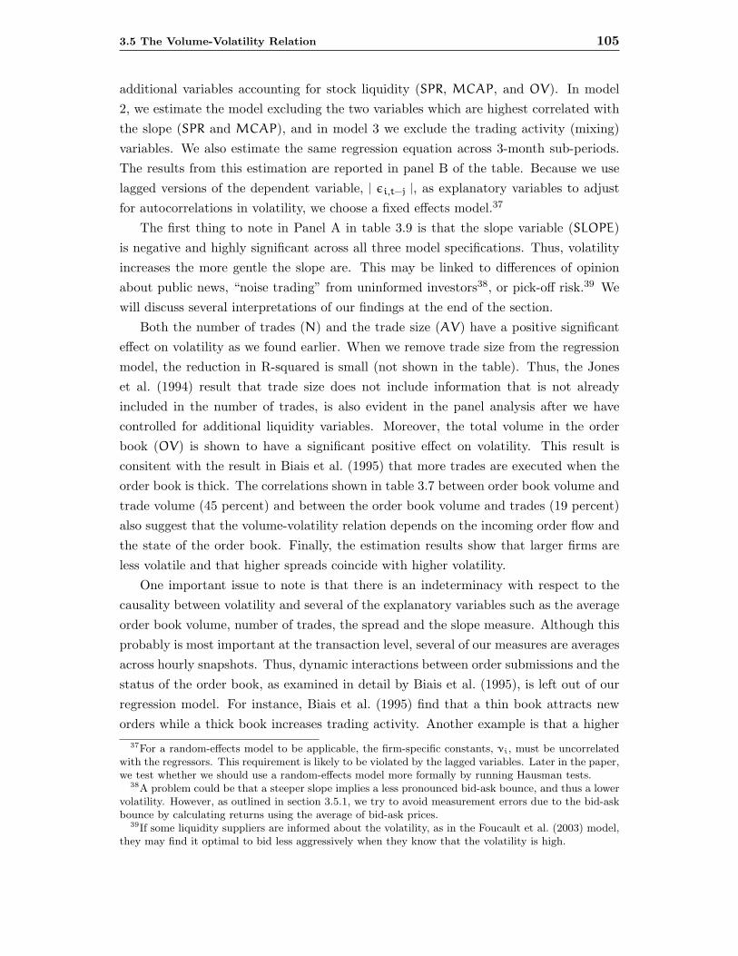
3.5 The Volume-Volatility Relation 105
additional variables accounting for stock liquidity (SPR, MCAP, and OV). In model2, we estimate the model excluding the two variables which are highest correlated withthe slope (SPR and MCAP), and in model 3 we exclude the trading activity (mixing)variables. We also estimate the same regression equation across 3-month sub-periods.The results from this estimation are reported in panel B of the table. Because we uselagged versions of the dependent variable, | εi,t−j |, as explanatory variables to adjustfor autocorrelations in volatility, we choose a fixed effects model.37
The first thing to note in Panel A in table 3.9 is that the slope variable (SLOPE)is negative and highly significant across all three model specifications. Thus, volatilityincreases the more gentle the slope are. This may be linked to differences of opinionabout public news, “noise trading” from uninformed investors38, or pick-off risk.39 Wewill discuss several interpretations of our findings at the end of the section.
Both the number of trades (N) and the trade size (AV) have a positive significanteffect on volatility as we found earlier. When we remove trade size from the regressionmodel, the reduction in R-squared is small (not shown in the table). Thus, the Joneset al. (1994) result that trade size does not include information that is not alreadyincluded in the number of trades, is also evident in the panel analysis after we havecontrolled for additional liquidity variables. Moreover, the total volume in the orderbook (OV) is shown to have a significant positive effect on volatility. This result isconsitent with the result in Biais et al. (1995) that more trades are executed when theorder book is thick. The correlations shown in table 3.7 between order book volume andtrade volume (45 percent) and between the order book volume and trades (19 percent)also suggest that the volume-volatility relation depends on the incoming order flow andthe state of the order book. Finally, the estimation results show that larger firms areless volatile and that higher spreads coincide with higher volatility.
One important issue to note is that there is an indeterminacy with respect to thecausality between volatility and several of the explanatory variables such as the averageorder book volume, number of trades, the spread and the slope measure. Although thisprobably is most important at the transaction level, several of our measures are averagesacross hourly snapshots. Thus, dynamic interactions between order submissions and thestatus of the order book, as examined in detail by Biais et al. (1995), is left out of ourregression model. For instance, Biais et al. (1995) find that a thin book attracts neworders while a thick book increases trading activity. Another example is that a higher
37For a random-effects model to be applicable, the firm-specific constants, νi, must be uncorrelatedwith the regressors. This requirement is likely to be violated by the lagged variables. Later in the paper,we test whether we should use a random-effects model more formally by running Hausman tests.
38A problem could be that a steeper slope implies a less pronounced bid-ask bounce, and thus a lowervolatility. However, as outlined in section 3.5.1, we try to avoid measurement errors due to the bid-askbounce by calculating returns using the average of bid-ask prices.
39If some liquidity suppliers are informed about the volatility, as in the Foucault et al. (2003) model,they may find it optimal to bid less aggressively when they know that the volatility is high.

106 Chapter 3 Order Book Characteristics and the Volume-Volatility Relation
volatility may reduce the number of orders coming into the market, which again lowersthe average slope of the book on that day. To examine this issues, we run simpleGranger causality tests between our slope measure and various order types and tradingactivity variables, both on an hourly and a daily frequency. Overall, we are unableto determine a clear one-way causality relation between the variables, rather we find atwo-way causality for most variable combinations.
The estimation results for models 2 and 3 are essentially the same as for model 1.The important thing to note is that the parameter estimate for SLOPE is significantlynegative and relatively stable across the three model specifications. The slope parame-ter is most negative and most significant in model 2, when we remove the spread (SPR)and market capitalization (MCAP) variables. This suggests that the slope capturesliquidity effects captured by these variables. Both the F-test of no firm-specific effects(firm-specific constants) and the Hausman specification test of whether a random-effectsmodel would be more appropriate relative to the fixed effects specification, are rejectedat the 1 percent level for all three models.40 This suggests that our firm-specific dummiesare correlated with the regressor, such that a fixed-effects specification is more appro-priate. The reason for this is that we have lagged versions of the dependent variable,which makes νi correlated with the regressors.
To examine the stability of the slope measure, we estimate model 1 for non-overlappingsub-periods of three months through the entire sample period. The results from theseregressions are reported in panel B in table 3.9. We only report the parameter estimatesand tests for the slope variable, number of trades, and trade size. The SLOPE param-eter is remarkably stable across the sub-samples. In addition, it is significant at the 1percent level within all sub-samples, except for the first. Also, the number of trades ishighly significant across all sub-periods while the average trade size is significant at the1 percent level only in half of the sub-sample regressions, suggesting that the number oftrades is the important component of volume in the volume-volatility relation, as alsosuggested by our analysis in section 3.5.1. The parameter estimate for the number oftrades decreases over the sample period. This is most likely due to the fact that themean number of trades across companies increases through the sample period.
F-tests of no fixed effects within each sub-period regression is rejected at the 1percent level.41 Our results suggest that both the order flow and the status of theorder book are significantly related to contemporaneous volatility in addition to tradingvolume.
40The Hausman test compares an inefficient but consistent OLS estimator (the fixed effects case) toan efficient GLS estimator (the random effects case). Thus, the Hausman test is a test of H0, thatrandom effects would be consistent and efficient, versus H1, that random effects would be inconsistent.Rejecting H0 would suggest that we should use a fixed effects specification.
41In addition, the Hausman test rejects a random effects specification at the 1 percent level for eachsub-sample model.
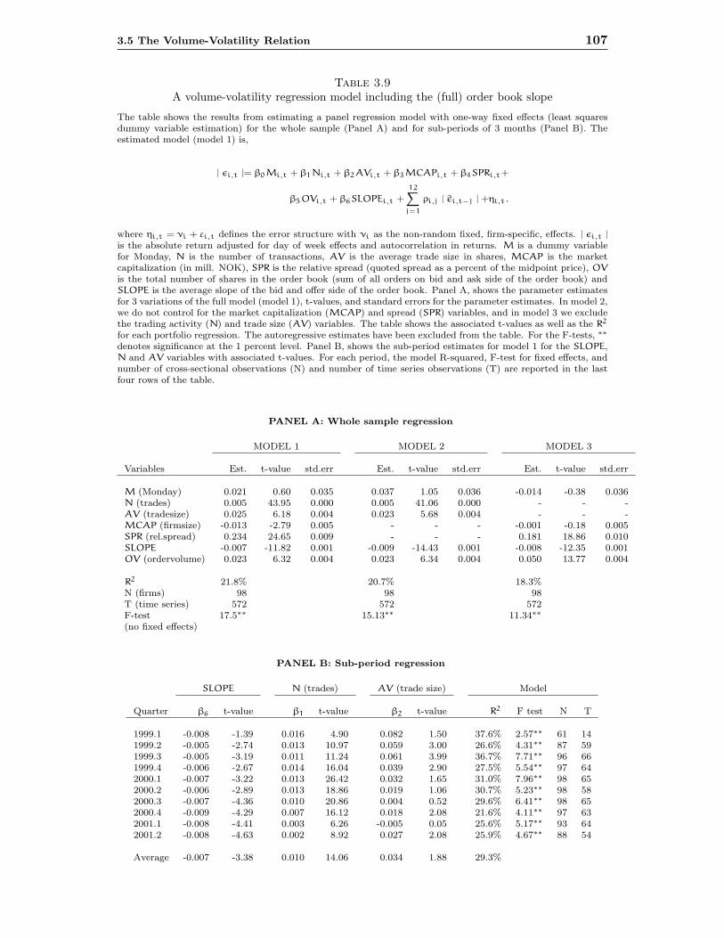
3.5 The Volume-Volatility Relation 107
Table 3.9A volume-volatility regression model including the (full) order book slope
The table shows the results from estimating a panel regression model with one-way fixed effects (least squaresdummy variable estimation) for the whole sample (Panel A) and for sub-periods of 3 months (Panel B). Theestimated model (model 1) is,
| εi,t |= β0Mi,t + β1Ni,t + β2AVi,t + β3MCAPi,t + β4SPRi,t+
β5OVi,t + β6SLOPEi,t +12∑
j=1
ρi,j | εi,t−j | +ηi,t.
where ηi,t = νi + εi,t defines the error structure with νi as the non-random fixed, firm-specific, effects. | εi,t |is the absolute return adjusted for day of week effects and autocorrelation in returns. M is a dummy variablefor Monday, N is the number of transactions, AV is the average trade size in shares, MCAP is the marketcapitalization (in mill. NOK), SPR is the relative spread (quoted spread as a percent of the midpoint price), OVis the total number of shares in the order book (sum of all orders on bid and ask side of the order book) andSLOPE is the average slope of the bid and offer side of the order book. Panel A, shows the parameter estimatesfor 3 variations of the full model (model 1), t-values, and standard errors for the parameter estimates. In model 2,we do not control for the market capitalization (MCAP) and spread (SPR) variables, and in model 3 we excludethe trading activity (N) and trade size (AV) variables. The table shows the associated t-values as well as the R2
for each portfolio regression. The autoregressive estimates have been excluded from the table. For the F-tests, ∗∗
denotes significance at the 1 percent level. Panel B, shows the sub-period estimates for model 1 for the SLOPE,N and AV variables with associated t-values. For each period, the model R-squared, F-test for fixed effects, andnumber of cross-sectional observations (N) and number of time series observations (T) are reported in the lastfour rows of the table.
PANEL A: Whole sample regression
MODEL 1 MODEL 2 MODEL 3
Variables Est. t-value std.err Est. t-value std.err Est. t-value std.err
M (Monday) 0.021 0.60 0.035 0.037 1.05 0.036 -0.014 -0.38 0.036N (trades) 0.005 43.95 0.000 0.005 41.06 0.000 - - -AV (tradesize) 0.025 6.18 0.004 0.023 5.68 0.004 - - -MCAP (firmsize) -0.013 -2.79 0.005 - - - -0.001 -0.18 0.005SPR (rel.spread) 0.234 24.65 0.009 - - - 0.181 18.86 0.010SLOPE -0.007 -11.82 0.001 -0.009 -14.43 0.001 -0.008 -12.35 0.001OV (ordervolume) 0.023 6.32 0.004 0.023 6.34 0.004 0.050 13.77 0.004
R2 21.8% 20.7% 18.3%N (firms) 98 98 98T (time series) 572 572 572F-test 17.5∗∗ 15.13∗∗ 11.34∗∗
(no fixed effects)
PANEL B: Sub-period regression
SLOPE N (trades) AV (trade size) Model
Quarter β6 t-value β1 t-value β2 t-value R2 F test N T
1999.1 -0.008 -1.39 0.016 4.90 0.082 1.50 37.6% 2.57∗∗ 61 141999.2 -0.005 -2.74 0.013 10.97 0.059 3.00 26.6% 4.31∗∗ 87 591999.3 -0.005 -3.19 0.011 11.24 0.061 3.99 36.7% 7.71∗∗ 96 661999.4 -0.006 -2.67 0.014 16.04 0.039 2.90 27.5% 5.54∗∗ 97 642000.1 -0.007 -3.22 0.013 26.42 0.032 1.65 31.0% 7.96∗∗ 98 652000.2 -0.006 -2.89 0.013 18.86 0.019 1.06 30.7% 5.23∗∗ 98 582000.3 -0.007 -4.36 0.010 20.86 0.004 0.52 29.6% 6.41∗∗ 98 652000.4 -0.009 -4.29 0.007 16.12 0.018 2.08 21.6% 4.11∗∗ 97 632001.1 -0.008 -4.41 0.003 6.26 -0.005 0.05 25.6% 5.17∗∗ 93 642001.2 -0.008 -4.63 0.002 8.92 0.027 2.08 25.9% 4.67∗∗ 88 54
Average -0.007 -3.38 0.010 14.06 0.034 1.88 29.3%
108 Chapter 3 Order Book Characteristics and the Volume-Volatility Relation
A robustness check In a limit order market, most trades originate from limit orders,i.e. there must be a strong relationship between order book shape, volatility and tradingvolume. One interpretation of our slope measure is that it is essentially a liquiditymeasure, and that the inner part of the order book is capturing the main effect onvolatility. A useful way to check this is to examine whether the slope calculated fromdifferent sets of the order book contain different information about volatility. One wayof doing this is to calculate the slope based on truncated versions of the order book.
We re-calculate the slope measure based on two different subsets of the book. Theresulting estimate distributions are shown in figure 3.6. Figure 3.6a shows the frequencydistribution of slope estimates calculated from an order book which is truncated to 5ticks away from the best quotes.42 Figure 3.6b shows the distribution of daily slopeestimates when we calculate the average slope based on twice as much of the order book(+/- 10 ticks). Finally, figure 3.6c shows the frequency distribution when we base ourslope estimates on the entire order book (+/- 100 ticks). The slope decreases the moreof the order book we use. This is expected, if the supply and demand curves in theorder book are concave.43 The mean slope when we use the full order book is about 37(median 28), while it increases to 57 (median 46) and 76 (median 62) when we calculateit from the order book truncated to +/- 10 and +/- 5 ticks respectively.
To examine whether the inner part of the order book captures the relationshipbetween volatility and slope, we re-estimate the regression models in table 3.9 withslope measures calculated from the two sub-sets of the order book. Panel A in table3.10 reports the estimation results. The results when we use the slope calculated fromthe order book truncated to +/- 10 ticks (SLOPE10) from the best quote on each sideare reported in model 1a, and the results when we truncate the order book to +/- 5 ticks(SLOPE5) are reported in model 1b. All other variables are identical to the previousanalysis. Panel B of the table shows the correlation between each slope measure andother variables. The main result from the estimation is that the slope parameter remainsnegative and significant. In addition, the parameter estimates become smaller comparedto the case where we used the full order book. The decrease in parameter size is mainlydue to the fact that the mean of the slope estimates increases (as shown in figure 3.6)while the dependent variable remains unchanged. Thus, the relationship seems to besimilar when we use only the inner levels of the order book to calculate the slope. AlsoR-squared of the different models does not change when we change the slope variable.Overall, our results suggest that the different slope measures capture mainly the samerelationship.
Panel B in table 3.10 shows the correlations between the three slope measures andthe activity and liquidity variables. One interesting thing to note is that the correlation
42That is, we use only the cumulative volume at the five first ticks on each side of the order bookwhen we calculate the average slope.
43Concave when we have price on the x-axis and volume on the y-axis.
3.5 The Volume-Volatility Relation 109
Figure 3.6 Frequency distribution of slope estimatesThe figures show the frequency distributions for (average) daily equally weighted normalized slope estimates for
all firms for the entire sample period. In figure (a) the slope calculations are calculated using only the first 5
levels of the order book, in figure (b) we use the first 10 levels of the order book and in figure (c) we use the
entire order book up to 100 tick levels.
( ;( M( d1( dE( 1(( 1;(
V%��s��SRjB}�
(
(�(;
(�(M
(�d1
(�dE
i�js�$%�SP��JZ�t
{kwxnS1MxSIs$jkSRjB}�S�R�$8s��RD w{DSV%��s��SRjB}�SL\TSd((S�${,RS
SSSSwPZjjSB�I��TABB,D
( ;( M( d1( dE( 1(( 1;(
V%��s��SRjB}�
(
(�(1
(�(;
(�(E
(�(M
(�d
i�js�$%�SP��JZ
�t{k
wxnS(nx
SIs$jk
SRjB}�S�R�$8s��RD wADSV%��s��SRjB}�SL\TSd(S�${,R
( ;( M( d1( dE( 1(( 1;(
V%��s��SRjB}�
(
(�(1
(�(;
(�(E
(�(M
i�js�$%�SP��JZ�t
{kwxdSEn;
SIs$jkSRjB}�S�R�$8s��RD
wsDSV%��s��SRjB}�SL\TSxS�${,R

110 Chapter 3 Order Book Characteristics and the Volume-Volatility Relation
between the slope and number of trades and between the slope and the trade volumein shares increases substantially the more we truncate the order book. This may reflectthat the relationship found in Biais et al. (1995), that a thicker (more concentrated)order book results in trades, is more pronounced when we evaluate the relationshipcloser to the inner quotes.
Table 3.11 shows the estimation results when estimating the model using the trun-cated slope measures across sub-periods. Similar to our findings when we estimate themodel over the whole sample period, we find that the size of the parameter estimateas well as its significance declines the more we truncate the order book. For model 1b,when we truncate the order book to 5 ticks, the slope estimate is only significantly dif-ferent from zero for half of the sub-samples. Thus, the significance of the slope variableis greatly reduced within sub-periods when we only use the inner part of the book. Notealso that when we use the slope based on the full order book, the relationship betweenvolatility and slope is stronger across sub-periods, as shown in panel B in table 3.9.
3.5.4 Number of trades and order book shape
In this sub-section, we examine the relationship between the slope and the contempo-raneous trading volume.
In table 3.12 we estimate a cross-sectional time series regression with the numberof trades as the dependent variable. As before, we control for liquidity variables whichare expected to be important with respect to the number of trades. When we base ourslope measure on the the full order book (model 1 in panel A), a significant negativerelationship between the slope and the number of trades is documented. Thus, the moregentle the order book slope, the higher the trading volume represented by the numberof trades. Models 2 and 3 in table 3.12 are estimated with slope measures calculatedfrom the truncated order books. Interestingly, we find that the parameter estimateswitches sign and becomes more positive the closer we get to the inner quotes. Thus,the slope at the inner quotes is positively related to the number of trades, while theaverage slope for the full book is negatively related to trade execution. In other words,the relationship between liquidity and trading activity becomes more evident when werestrict the analysis to the inner part of the order book.
We also find that the number of trades is lower on Mondays, that the average tradesize is unrelated to the number of trades, and that larger firms are more frequentlytraded. In addition, we find that there is less trading when the quoted percentagespread is large, and that there are more trades when the volume of shares in the orderbook is high. Again, one caveat with respect to the analysis is that we do not take intoaccount the dynamic interactions between the order flow and status of the order book.For example, as found by Biais et al. (1995), a thinner book may attract new orderswhich in the next step increases the number of transactions. The most interesting result
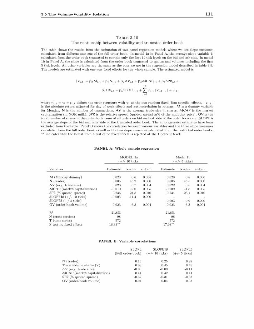
3.5 The Volume-Volatility Relation 111
Table 3.10The relationship between volatility and truncated order book
The table shows the results from the estimation of two panel regression models where we use slope measurescalculated from different sub-sets of the full order book. In model 1a in Panel A, the average slope variable iscalculated from the order book truncated to contain only the first 10 tick levels on the bid and ask side. In model1b in Panel A, the slope is calculated from the order book truncated to quotes and volumes including the first5 tick levels. All other variables are the same as the ones we use in the regression model described in table 3.9.The models are estimated with one-way fixed effects for the whole sample. The estimated model is,
| εi,t |= β0Mi,t + β1Ni,t + β2AVi,t + β3MCAPi,t + β4SPRi,t+
β5OVi,t + β6SLOPEi,t +12∑
j=1
ρi,j | εi,t−j | +ηi,t.
where ηi,t = νi + εi,t defines the error structure with νi as the non-random fixed, firm specific, effects. | εi,t |is the absolute return adjusted for day of week effects and autocorrelation in returns. M is a dummy variablefor Monday, N is the number of transactions, AV is the average trade size in shares, MCAP is the marketcapitalization (in NOK mill.), SPR is the relative spread (quoted spread as% of the midpoint price), OV is thetotal number of shares in the order book (sum of all orders on bid and ask side of the order book) and SLOPE isthe average slope of the bid and offer side of the truncated order book. The autoregressive estimates have beenexcluded from the table. Panel B shows the correlation between various variables and the three slope measurescalculated from the full order book as well as the two slope measures calculated from the restricted order books.∗∗ indicates that the F-test from a test of no fixed effects is rejected at the 1 percent level.
PANEL A: Whole sample regression
MODEL 1a Model 1b(+/- 10 ticks) (+/- 5 ticks)
Variables Estimate t-value std.err Estimate t-value std.err
M (Monday dummy) 0.023 0.6 0.035 0.028 0.8 0.036N (trades) 0.005 45.2 0.000 0.005 45.5 0.000AV (avg. trade size) 0.023 5.7 0.004 0.022 5.5 0.004MCAP (market capitalization) -0.010 -2.0 0.005 -0.009 -1.8 0.005SPR (% quoted spread) 0.236 24.8 0.010 0.234 23.1 0.010SLOPE10 (+/- 10 ticks) -0.005 -11.4 0.000 - - -SLOPE5 (+/-5 ticks) - - - -0.003 -9.9 0.000OV (order-book volume) 0.023 6.3 0.004 0.023 6.3 0.004
R2 21.8% 21.8%N (cross section) 98 98T (time series) 572 572F-test no fixed effects 18.33∗∗ 17.93∗∗
PANEL B: Variable correlations
SLOPE SLOPE10 SLOPE5(Full order-book) (+/- 10 ticks) (+/- 5 ticks)
N (trades) 0.13 0.25 0.28Trade volume shares (V) 0.08 0.45 0.45AV (avg. trade size) -0.08 -0.09 -0.11MCAP (market capitalization) 0.44 0.42 0.41SPR (% quoted spread) -0.32 -0.31 -0.33OV (order-book volume) 0.04 0.04 0.03

112 Chapter 3 Order Book Characteristics and the Volume-Volatility Relation
Table 3.11The relationship between volatility truncate order book across sub-periods
The table shows the results from estimating the two panel regression model in table 3.10 for sub-periods of threemonths. In model 1a, the average slope variable is calculated using an order book truncated to the first 10 ticklevels on the bid and ask side. In model 1b, the average slope is calculated using an order book truncated toprices and volumes within the first 5 tick levels. All other variables are the same as the variables used in table3.9. The models are estimated with one-way fixed effects for each sub-period. The estimated model is,
| εi,t |= β0Mi,t + β1Ni,t + β2AVi,t + β3MCAPi,t + β4SPRi,t+
β5OVi,t + β6SLOPEi,t +
12∑j=1
ρi,j | εi,t−j | +ηi,t.
where ηi,t = νi + εi,t defines the error structure with νi as the non-random fixed, firm-specific, effects. | εi,t |
is the absolute return adjusted for day of week effects and autocorrelation in returns. M is a dummy variable
for Monday, N is the number of transactions, AV is the average trade size in shares, MCAP is the market
capitalization (in NOK mill.), SPR is the relative spread (quoted spread as% of the midpoint price), OV is the
total number of shares in the order book (sum of all orders on bid and ask side of the order book) and SLOPE is
the average slope of the bid and offer side of the restricted order book. The table shows the parameter estimates
for 2 variations of model 1 in table 3.9 with the associated t-value, std.error of the estimate, the model R-squared.
∗∗ indicates that the F-test for no fixed effects is rejected at the 1 percent level.
Model 1a Model 1b(+/- 10 ticks) (+/- 5 ticks)
Quarter SLOPE10 t-val. std.err R2 F-val. SLOPE5 t-val. std.err R2 F-val.
1999.1 0.000 -0.1 0.004 39% 3.4∗∗ -0.003 -1.1 0.003 31% 2.2∗∗
1999.2 -0.004 -2.4 0.002 27% 4.2∗∗ -0.001 -0.9 0.001 27% 4.5∗∗
1999.3 -0.002 -1.6 0.001 33% 5.2∗∗ -0.001 -0.7 0.001 34% 5.0∗∗
1999.4 -0.003 -1.7 0.002 28% 6.1∗∗ -0.001 -1.1 0.001 28% 6.5∗∗
2000.1 -0.004 -2.6 0.001 31% 8.4∗∗ -0.002 -1.9 0.001 31% 8.5∗∗
2000.2 -0.003 -2.4 0.001 30% 5.1∗∗ -0.002 -2.0 0.001 30% 5.1∗∗
2000.3 -0.003 -2.8 0.001 31% 6.9∗∗ -0.001 -1.2 0.001 31% 6.8∗∗
2000.4 -0.006 -4.6 0.001 24% 4.1∗∗ -0.005 -4.2 0.001 24% 4.0∗∗
2001.1 -0.004 -3.1 0.001 26% 5.2∗∗ -0.003 -2.6 0.001 26% 5.2∗∗
2001.2 -0.006 -4.0 0.001 25% 4.8∗∗ -0.004 -3.3 0.001 26% 4.8∗∗
Average -0.004 -2.5 0.002 29.4% -0.002 -1.9 0.001 28.8%

3.5 The Volume-Volatility Relation 113
from the estimation is that a slope measure calculated on the basis of the full order bookseems to provide different information compared to a slope measure calculated on thebasis of the volume at the inner quotes.
In the previous sub-section, we found that the relationship between price volatilityand the slope was well proxied by a slope measure based on the inner part of the book.In this section, we have documented a significant difference between slope measuresbased on different order book truncations.
3.5.5 Interpretation of the results
The relationships documented in this study are interesting in several respects. First,although most of the activity occur at the inner part of the order book, the orderbook data shows that the liquidity provided at the inner quotes in many cases reflectonly a modest part of the total liquidity supplied in the full order book. Second, thecharacteristics of the order book vary systematically over the trading day as well asacross firms. Third, as far as we know, no previous studies have examined in detail therelationship between the characteristics of the full order book and volume and volatilityin a cross-sectional time series setting.
One question is why orders persist further out in the book? One reason may be thattraders are slow in revising their orders in response to new information. Another reasonsuggested by Sandas (2001) is that the placement of orders deep in the book are based onstrategic choices where, in a multi-period setting, the gains from obtaining price priorityof the orders further out in the book are traded off the costs of monitoring them. Whenwe examine the slopes of the order books across companies over time, we find that thereare marked differences across firms in the amount of volume provided throughout theorder book, and that these differences persist through time. As shown in table 3.8 somefirms have generally a very large fraction of their liquidity concentrated close to the bestquotes, while other firms have a relatively larger fraction of the order volume furtherout in the book. A second question is why such differences in slope estimates acrossfirms appear? The systematic patterns found may indicate that the shape of the orderbook capture some underlying characteristics of the the trading strategies of liquiditysuppliers across firms. One possible explanation is related to asymmetric information.In general, we find that smaller firms have order books with a gentler slope than largerfirms, which is in line with the hypothesis that there is more private information insmaller than in larger firms.
In summary, our main findings about the relationship between the slope of the bookand the volume-volatility relation are;
• A more gentle slope (more dispersed order book) coincide with a higher volatilityacross firms and over time.
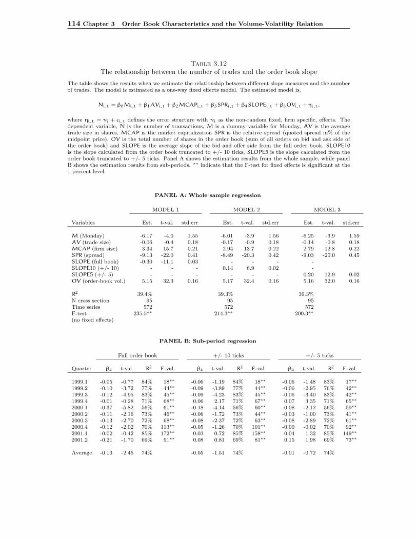
114 Chapter 3 Order Book Characteristics and the Volume-Volatility Relation
Table 3.12The relationship between the number of trades and the order book slope
The table shows the results when we estimate the relationship between different slope measures and the numberof trades. The model is estimated as a one-way fixed effects model. The estimated model is,
Ni,t = β0Mi,t + β1AVi,t + β2MCAPi,t + β3SPRi,t + β4SLOPEi,t + β5OVi,t + ηi,t.
where ηi,t = νi + εi,t defines the error structure with νi as the non-random fixed, firm specific, effects. Thedependent variable, N is the number of transactions, M is a dummy variable for Monday, AV is the averagetrade size in shares, MCAP is the market capitalization SPR is the relative spread (quoted spread in% of themidpoint price), OV is the total number of shares in the order book (sum of all orders on bid and ask side ofthe order book) and SLOPE is the average slope of the bid and offer side from the full order book, SLOPE10is the slope calculated from the order book truncated to +/- 10 ticks, SLOPE5 is the slope calculated from theorder book truncated to +/- 5 ticks. Panel A shows the estimation results from the whole sample, while panelB shows the estimation results from sub-periods. ∗∗ indicate that the F-test for fixed effects is significant at the1 percent level.
PANEL A: Whole sample regression
MODEL 1 MODEL 2 MODEL 3
Variables Est. t-val. std.err Est. t-val. std.err Est. t-val. std.err
M (Monday) -6.17 -4.0 1.55 -6.01 -3.9 1.56 -6.25 -3.9 1.59AV (trade size) -0.06 -0.4 0.18 -0.17 -0.9 0.18 -0.14 -0.8 0.18MCAP (firm size) 3.34 15.7 0.21 2.94 13.7 0.22 2.79 12.8 0.22SPR (spread) -9.13 -22.0 0.41 -8.49 -20.3 0.42 -9.03 -20.0 0.45SLOPE (full book) -0.30 -11.1 0.03 - - - -SLOPE10 (+/- 10) - - - 0.14 6.9 0.02 -SLOPE5 (+/- 5) - - - - - - 0.20 12.9 0.02OV (order-book vol.) 5.15 32.3 0.16 5.17 32.4 0.16 5.16 32.0 0.16
R2 39.4% 39.3% 39.3%N cross section 95 95 95Time series 572 572 572F-test 235.5∗∗ 214.3∗∗ 200.3∗∗
(no fixed effects)
PANEL B: Sub-period regression
Full order book +/- 10 ticks +/- 5 ticks
Quarter β4 t-val. R2 F-val. β4 t-val. R2 F-val. β4 t-val. R2 F-val.
1999.1 -0.05 -0.77 84% 18∗∗ -0.06 -1.19 84% 18∗∗ -0.06 -1.48 83% 17∗∗
1999.2 -0.10 -3.72 77% 44∗∗ -0.09 -3.89 77% 44∗∗ -0.06 -2.95 76% 42∗∗
1999.3 -0.12 -4.95 83% 45∗∗ -0.09 -4.23 83% 45∗∗ -0.06 -3.40 83% 42∗∗
1999.4 -0.01 -0.28 71% 68∗∗ 0.06 2.17 71% 67∗∗ 0.07 3.35 71% 65∗∗
2000.1 -0.37 -5.82 56% 61∗∗ -0.18 -4.14 56% 60∗∗ -0.08 -2.12 56% 59∗∗
2000.2 -0.11 -2.16 73% 46∗∗ -0.06 -1.72 73% 44∗∗ -0.03 -1.00 73% 41∗∗
2000.3 -0.13 -2.70 72% 68∗∗ -0.08 -2.37 72% 63∗∗ -0.08 -2.89 72% 61∗∗
2000.4 -0.12 -2.02 70% 113∗∗ -0.05 -1.26 70% 101∗∗ -0.00 -0.02 70% 92∗∗
2001.1 -0.02 -0.42 85% 172∗∗ 0.03 0.72 85% 158∗∗ 0.04 1.32 85% 149∗∗
2001.2 -0.21 -1.70 69% 91∗∗ 0.08 0.81 69% 81∗∗ 0.15 1.98 69% 73∗∗
Average -0.13 -2.45 74% -0.05 -1.51 74% -0.01 -0.72 74%

3.5 The Volume-Volatility Relation 115
• The relationship between the number of trades and the slope of the book dependson which subset of the order book is used.
– When we use the slope from the inner book (+/- 5 ticks) there is a positiverelationship in which a steep slope coincide with a high number of trades.
– When the entire order book is used (+/- 100 ticks), the relationship is re-versed, i.e. a more gentle slope coincide with a higher number of trades.
One interesting interpretation of these results is that the differences in the limit orderbooks across firms reflect valuation uncertainty and heterogenous valuations among theliquidity suppliers. Although no models exist that offer any predictions to how thefull limit order book would look like in a market with heterogenous liquidity suppli-ers, models assuming strategic behavior of uninformed investors provide an interestingframework which could motivate such an interpretation. Shalen (1993) shows that thestrategic behavior of liquidity traders may be an important contributor to both volumeand volatility in addition to information arrivals. In her model, when uninformed in-vestors has dispersed beliefs about asset values, they are faced with a signal extractionproblem, making them react to all types of trades in the order-flow which may or maynot be related to informed trading. Due to this, they increase both trading volume andprice volatility above what would be expected in equilibrium. Thus, the relationshipbetween volume and volatility is not merely due to the information arrival process (asin the mixture of distributions framework), but also due to strategic trading by unin-formed traders. The higher the fraction of uninformed traders in the population, thegreater the dispersion of beliefs, and the greater the excess volume and excess volatility.
Valuation uncertainty (dispersion of beliefs) may to some degree be captured by theshape of the order book, as different levels of the book reflect the reservation prices ofliquidity suppliers. This provides an interesting interpretation for why the order volumesobserved in the limit order book are more dispersed than predicted by theoretical modelssuch as Glosten (1994). If the uncertainty about the value of a firm is high and liquiditytraders differ in their private valuations, they may submit their orders across a widerrange of prices relative to the case when there is greater agreement about the true value,cf the example in figure 3.2 where we show the difference in the average order booksbetween two companies which obviously differ in their valuation uncertainty.
If valuation uncertainty coincide with a more gentle order book slope, our resultssupport several predictions from Shalen (1993). First, increased dispersion of beliefsis predicted to increase (excess) trading volume. Our finding that a more gentle slopecoincide with a greater number of trades is in line with this prediction. Second, a peakvolume and volatility is predicted at the beginning of the trading day because dispersionof beliefs is greater when the price signal is more noisy. As shown in section 3.4, theslope of the order book is relatively more gentle in the beginning of the trading day
116 Chapter 3 Order Book Characteristics and the Volume-Volatility Relation
than later in the day. However, this feature of the data may also be due to adjustmentsin liquidity demand.
There are also models that relate the status of the order book to the order submissionstrategies of homogeneous liquidity providers and how they provide the limit order bookwhen there is a probability of informed trading. If one takes the one period modelby Glosten (1994) as a benchmark, the slope of the supply and demand schedules inthe order book results from the probability of informed trading. Sandas (2001) teststhe predictions in Glosten (1994) in the Swedish market which is very similar to theNorwegian market. He finds strong evidence that there is insufficient depth in theobserved order book relative to the theoretical prediction. In other words, the slope ofthe demand and supply schedules in the order book, at the inner quotes, is much toogentle to be explained by theory.
Our results for the inner part of the order book are consistent with models where ahigher liquidity at the inner quotes increases the number of trades. However, our resultsfor the full order book provide some additional results that are not captured by anytheoretical model. Our finding that the volume and volatility in financial markets maybe affected by valuation uncertainty and heterogenous beliefs among liquidity suppliersprovides a motivation for future research on this topic. From a more practical point ofview, the discussions in the popular press about the value of companies, and sometimesvery different buy and sell recommendations by analysts for the same stock, suggestthat the differences in valuations may be an important factor driving trading activityin financial markets.

3.6 Conclusion 117
3.6 Conclusion
A positive correlation between price volatility and trading volume has been documentedin a variety of studies. Investigating plausible explanations for this relation is impor-tant because it can enhance our understanding of how information is disseminated intomarket prices.
There are two, mainly complementary, hypotheses relating trading volume andvolatility. The mixture of distributions hypothesis states that the volume-volatilityrelation is driven by a directing process that can be interpreted as the flow of informa-tion. The dispersion of beliefs hypothesis states that both trading volume and volatilityshould be higher the greater the dispersion of beliefs about security values among in-vestors. One explanation behind this statement is based on asymmetric information andstrategic investor behavior. Uninformed traders cannot distinguish informed trades fromliquidity trades, and by reacting to trades with no information content, they increaseboth volume and volatility relative to equilibrium values in a situation with symmetricinformation. A positive relation between dispersion of beliefs and the volume-volatilityrelation can also be explained in a non-informational setting where investors have differ-ent opinions about the value of the same news. Thus, while the mixture of distributionshypothesis states that trading volume and price movements result from new informationarrivals, the dispersion of beliefs hypothesis also relates a part of the volume-volatilityrelation to increased trading by uninformed traders or symmetrically informed investorswho disagree on the same news.
Using a detailed data sample from the Oslo Stock Exchange (OSE), we examinewhether information about the volume-volatility relation is contained in the shape of alimit order book. We first document that our data exhibit a standard volume-volatilityrelation. Moreover, we show that the result in Jones et al. (1994), that the average sizeof trades has little marginal explanatory power when volatility is conditioned on thenumber of daily transactions, also applies in a limit order market. A unique feature ofour data sample is that we can rebuild the whole order book at any time during thetrading day. This enables us to investigate whether the characteristics of the limit orderbook contain information about the volume-volatility relation.
Our main findings show that more gentle demand and supply schedules increasesvolatility and trading volume in a cross-sectional time series setting. One possibleinterpretation of this is that the number of trades is not a proxy for the mixing variable,but the mixing variable itself as suggested in models with heterogenous agents.

118 Chapter 3 Order Book Characteristics and the Volume-Volatility Relation
3.A Calculating slope measures
To explain the slope calculation more specifically, let NA and NB be respectively thetotal number of bid and ask prices (tick levels) containing orders. Let τ denote thetick level, with τ = 1 representing the best quote with a positive volume. Furthermore,let pB
1 and pA1 be respectively the best bid and ask prices, and pM denote the bid-
ask midpoint (which is the average of pB1 and pA
1 ). Let vBτ and vA
τ be respectively thepercentage of total share volume at each tick level on the bid and ask side of the book.E.g. vA
τ=1=0.1 would mean that 10% of the total number of shares supplied on the askside of the order book is located at the best ask quote at that point in time. Finally, letωB
τ and ωAτ denote the weight of the local slope calculated at tick level τ for respectively
the bid and the ask side of the book. These weights are set equal in the case when weequally weight the local slopes across all tick levels. In the case when we weight eachlocal slope differently, we use a simple linear weighting scheme where the weight at eachtick level, τ, is calculated as,
ωAτ =
|τmax| − |τ| + 1∑τ(|τ
max| − |τ|) + 1(3A.1)
for the ask side, and similarly for the bid side. τmax is the maximum tick level withnon-zero volume. Thus, the quotes which are the furthest out in the order book (e.g. atτ=80) get a relatively smaller weight than orders closer to the midpoint (e.g. at τ=10).The summation is done across all ticks with a non-zero volume. This ensures that theweights sum to one on each side of the book.
The average elasticity for the supply curve, SE, on day t at snapshot time s ∈ [1..6]
for company i can then be represented as,
SEsi,t =
{vA
1
pA1 /pM − 1
ωAi,1 +
NA∑τ=1
vAτ+1/vA
τ − 1
pAτ+1/pA
τ − 1ωA
i,τ
}(3A.2)
Similarly, the demand curve, DE, can be represented as,
DEsi,t =
{vB
1
| pB1 /pM − 1 |
ωBi,1 +
NB∑τ=1
vBτ−1/vB
τ − 1
| pBτ−1/pB
τ − 1 |ωB
i,τ
}(3A.3)
The first term of both equations expresses the slope between the bid-ask midpoint andthe best bid and ask prices, while the second term of both equations expresses the sumof the local elasticities for the rest of the order book. The average elasticity in the orderbook at snapshot s is just the average of SEs
i,t and DEsi,t,
3.B Balanced sample estimation 119
SLOPEsi,t =
SEsi,t + DEs
i,t
2(3A.4)
The order book is rebuilt at 10:30, 11:30, 12:30, 13:30, 14:30 and 15:30 each tradingday for each firm. We exclude order volume above/below 100 ticks away from the innerquotes. For a stock trading at NOK 100 with a minimum tick size of NOK 0.5 thiswould mean that orders above NOK 150 and below NOK 50 are excluded from ourcalculations. Also, if we based our estimates of daily elasticities on one snapshot only(e.g. at noon), they could be biased due to large trades having temporarily reduced theliquidity of one side of the book or systematic time of day effects. To obtain a less noisyrepresentation of the average daily supply and demand curves for each firm on eachdate, we therefore average the slopes across the 6 snapshots, i.e.
SLOPEi,t =1
6
6∑s=1
SLOPEsi,t (3A.5)
3.B Balanced sample estimation
To examine the robustness of our results, we restrict our sample to firms that weretraded every day through the sample period of 572 trading days. This leaves us witha balanced sample of 25 firms with 572 time series observations each. In addition, thefiltering leaves us with a sample of the largest, most liquid and actively traded firmson the exchange. If the previous results are mainly due to noise or outliers introducedby small illiquid firms or the unbalanced dataset, the balancing of the sample shouldreveal this. In table 3.B1 we re-estimate model 1 in panel A of table 3.9 and model 1aand 1b in panel A of table 3.10 for the balanced sample. The estimation results arequantitatively similar to the results when we use the full sample. Most interestingly,the parameter estimate for SLOPE is negative and of similar size as before. In addition,the SLOPE estimate becomes smaller (less negative) the more we truncate the orderbook. As before, this is mainly due to the increase in the size of the slope estimates themore the order book is truncated. The largest difference between the models estimatedfor the balanced and unbalanced sample is that the R-squared of the models is muchhigher for the balanced sample, suggesting that there is more noise in the unbalancedsample.
In table 3.B2 we re-estimate the model for trading activity in panel A of table 3.12for the balanced sample. Although the parameter estimates change more in size thanwhat was the case for the volatility models, the parameters are qualitatively similar.Most importantly, the SLOPE parameter estimate is negative when it is calculated usingthe full order book, and becomes increasingly more positive the more the order bookis truncated. Thus, also for the balanced sample, the results suggests that the more

120 Chapter 3 Order Book Characteristics and the Volume-Volatility Relation
Table 3.B1Volatility/slope regression with balanced data sample
The table shows the estimation results of a cross-sectional time series model for the relationship between differentslope measures and the daily volatility when using a balanced sample. The models are similar to those estimated(for the unbalanced sample) in table 3.9 (Model 1) and table 3.10. The estimated model is,
| εi,t |= β0Mi,t + β1Ni,t + β2AVi,t + β3MCAPi,t + β4SPRi,t + β5OVi,t + β6SLOPEi,t +12∑
j=1
ρi,j | εi,t−j | +ηi,t.
where ηi,t = νi + εi,t defines the error structure with νi as the non-random fixed, firm-specific, effects. | εi,t |is the absolute daily return, N is the number of transactions, M is a dummy variable for Monday, AV is theaverage trade size in shares, MCAP is the market capitalization (in NOK mill.), SPR is the relative spread(quoted spread as % of the midpoint price), OV is the total number of shares in the order book (sum of allorders on bid and ask side of the order book) and SLOPE is the average slope of the bid and offer side from thefull order book, SLOPE10 is the slope calculated from the order book truncated to +/- 10 ticks, SLOPE5 is theslope calculated from the order book truncated to +/- 5 ticks. | εi,t−j | are lagged absolute returns to take intoaccount autocorrelations.
PANEL A: Volatility/slope regressions for balanced sample
Volatility/slope Volatility/slope Volatility/slope(full book) (+/- 10 ticks) (+/- 5 ticks)
Variables Est. t-value std.err Est. t-value std.err Est. t-value std.err
M (monday dummy) -0.083 -1.5 0.057 -0.081 -1.4 0.057 -0.078 -1.4 0.057N (trades) 0.004 34.6 0.000 0.004 35.6 0.000 0.004 35.7 0.000AV (avg. trade size) 0.017 2.5 0.007 0.014 2.0 0.007 0.013 1.9 0.007MCAP (market cap.) -0.015 -2.7 0.006 -0.009 -1.6 0.006 -0.008 -1.4 0.006SPR (% quoted spread) 0.345 16.3 0.021 0.358 16.9 0.021 0.351 16.6 0.021SLOPE (full book) -0.008 -10.0 0.001 - - - - - -SLOPE10 (+/- 10 ticks) - - - -0.007 -10.6 0.001 - - -SLOPE5 (+/-5 ticks) - - - - - - -0.005 -9.6 0.001OV (order book volume) 0.011 3.1 0.004 0.010 3.0 0.004 0.011 3.0 0.004
R2 37.6% 37.6% 37.5%N (cross section) 25 25 25T (time series) 572 572 572F-test (no fixed effects) 41.6∗∗ 41.2∗∗ 40.9∗∗
dispersed prices are across the order book, the more trades are executed. Furthermore,when the slope is calculated from the truncated order book, only using the volume atthe inner levels of the book, the results suggests that a thick book coincides with hightrading activity.
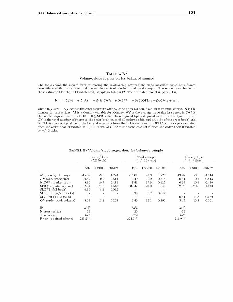
3.B Balanced sample estimation 121
Table 3.B2Volume/slope regression for balanced sample
The table shows the results from estimating the relationship between the slope measures based on differenttruncations of the order book and the number of trades using a balanced sample. The models are similar tothose estimated for the full (unbalanced) sample in table 3.12. The estimated model in panel B is,
Ni,t = β0Mi,t + β1AVi,t + β2MCAPi,t + β3SPRi,t + β4SLOPEi,t + β5OVi,t + ηi,t.
where ηi,t = νi + εi,t defines the error structure with νi as the non-random fixed, firm-specific, effects. N is thenumber of transactions, M is a dummy variable for Monday, AV is the average trade size in shares, MCAP isthe market capitalization (in NOK mill.), SPR is the relative spread (quoted spread as % of the midpoint price),OV is the total number of shares in the order book (sum of all orders on bid and ask side of the order book) andSLOPE is the average slope of the bid and offer side from the full order book, SLOPE10 is the slope calculatedfrom the order book truncated to +/- 10 ticks, SLOPE5 is the slope calculated from the order book truncatedto +/- 5 ticks.
PANEL B: Volume/slope regressions for balanced sample
Trades/slope Trades/slope Trades/slope(full book) (+/- 10 ticks) (+/- 5 ticks)
Est. t-value std.err Est. t-value std.err Est. t-value std.err
M (monday dummy) -15.05 -3.6 4.224 -14.01 -3.3 4.227 -13.98 -3.3 4.216AV (avg. trade size) -0.50 -0.9 0.514 -0.49 -0.9 0.514 -0.34 -0.7 0.513MCAP (market cap.) 8.10 19.7 0.411 7.41 17.8 0.417 6.89 16.4 0.420SPR (% quoted spread) -32.39 -21.0 1.543 -32.47 -21.0 1.545 -32.07 -20.8 1.540SLOPE (full book) -0.50 -8.1 0.062 - - - - - -SLOPE10 (+/- 10 ticks) - - - 0.33 6.7 0.049 - - -SLOPE5 (+/- 5 ticks) - - - - - - 0.44 11.3 0.039OV (order book volume) 3.33 12.8 0.262 3.43 13.1 0.262 3.45 13.2 0.261
R2 33% 33% 34%N cross section 25 25 25Time series 572 572 572F-test (no fixed effects) 233.2∗∗ 224.0∗∗ 211.9∗∗
122 Chapter 3 Order Book Characteristics and the Volume-Volatility Relation
3.C An alternative slope measure and separating the bid/ask
side
As a final exercise, we examine whether the weighted slope estimate, where we weighteach local slope with the distance from the inner quote (tick-weighted slope)44, changesour results. The two slope measures are highly correlated (98%) so we do not expectto see any large differences. However, in addition to examining the alternative slopeestimate, we also estimate the effect of the slope of the bid and ask side of the orderbook separately, both in the balanced and unbalanced case as well as for the varioustruncations of the order book. In table 3.C1 we report slope estimates for the volatilityregressions, and in panel B we report slope estimates for the trading activity regressions.To preserve space we only report the slope estimates for the average slope, the bid andask slope as well as the p-value from an F-test for equality between the slope estimatefor the bid and ask side.
Starting with the first column (slope calculated from the full order book), we see thatthe estimate for both the equally weighted slope and the tick-weighted slope are negativeand significant both for in the balanced and unbalanced case. The main difference isthat the weighted slope estimate is more negative than for the equally weighted estimate.Furthermore, when examining the slope estimates for the bid and ask side separately,they are only significantly different at the 5% level for the tick-weighted slope in theunbalanced case. In the two next columns (when we use the truncated order books forcalculating the slope) the results are essentially similar, in the sense that the parameterestimate for the tick-weighted slope is more negative than for the equally weighted slope.Both slopes become less negative the more the order book is truncated. With respectto differences between the ask and bid slopes, the parameter estimates are significantlydifferent at the 5% and 10% level for both measures in the balanced case, while theyare not different in the unbalanced case.
In table 3.C2 we perform a similar analysis for the trading activity regressions.Looking first at the first column (slope calculated from the full order book), we seethat the parameter estimate is significantly negative both for the equally weighted andtick-weighted slope in the balanced and unbalanced case. Thus, in both cases a moredispersed order book coincides with high trading activity. Interestingly, for the equallyweighted slope (both in the balanced and unbalanced case) the ask slope estimate issignificantly positive while it is significantly negative for the bid slope. For both slopemeasures, the bid slope is more significant than the ask slope in explaining the numberof trades. This may reflect the asymmetry in the order book. With respect to ourinterpretation of the slope as potentially proxying for dispersion, it may reflect thatthe bid side of the market is more important with respect to dispersion of beliefs,
44See appendix 3.A for explanation.

3.C An alternative slope measure and separating the bid/ask side 123
Table 3.C1Alternative slope measures and the effect of bid and ask slope on volatility
The table shows slope estimates from the volatility/slope regressions for the equally weighted slope measure andtick-weighted slope measure calculated from different order book truncations in the balanced and unbalancedsample.
Volatility/slope Volatility/slope Volatility/slope(full book) (+/- 10 ticks) (+/- 5 ticks)
Estimate t-value Estimate t-value Estimate t-valueBalanced sample:Equally weighted slope (SLOPE) -0.008 -10.0 -0.007 -10.6 -0.005 -9.6
-Ask slope -0.006 -4.0 -0.005 -6.2 -0.004 -6.2-Bid slope -0.004 -8.8 -0.003 -7.3 -0.002 -5.2
p-value (bid-ask=0) 0.22 0.03 0.01
Tick-weighted slope -0.016 -9.5 -0.014 -9.8 -0.010 -8.9-Ask slope -0.008 -1.8 -0.012 -4.8 -0.008 -4.8-Bid slope -0.008 -9.0 -0.006 -7.6 -0.004 -5.9
p-value (bid-ask=0) 0.97 0.03 0.06
Estimate t-value Estimate t-value Estimate t-valueFull sample:Equally weighted slope (SLOPE) -0.007 -11.8 -0.005 -11.4 -0.003 -9.9
-Ask slope -0.002 -2.3 -0.003 -5.9 -0.002 -5.8-Bid slope -0.004 -11.4 -0.002 -8.1 -0.001 -5.8
p-value (bid-ask=0) 0.07 0.54 0.23
Tick-weighted slope -0.015 -11.5 -0.010 -10.4 -0.006 -8.8-Ask slope -0.001 -0.4 -0.004 -3.6 -0.003 -3.5-Bid slope -0.008 -11.5 -0.005 -8.8 -0.003 -6.8
p-value (bid-ask=0) 0.02 0.62 0.60
while the ask side may be more related to liquidity supply. Furthermore, when weexamine the parameter estimates, both for the equally weighted and tick-weighted slopeestimates, for the slope measures calculated from the truncated order books (in the lasttwo columns), we see that the importance of the ask slope increases while the bid slopebecomes more positive and less significant. This is in line with an interpretation, thatthe ask side is important in facilitating trading (and may capture increased tradingactivity by impatient liquidity traders) while the bid side reflects valuation uncertainty.

124 Chapter 3 Order Book Characteristics and the Volume-Volatility Relation
Table 3.C2Alternative slope measures and the effect of bid and ask slope on trading activity
The table show slope estimates from the trading activity/slope regressions for the equally weighted slope measureand tick-weighted slope measure calculated from different order book truncations in the balanced and unbalancedsample.
Trades/slope Trades/slope Trades/slope(full book) (+/- 10 ticks) (+/- 5 ticks)
Estimate t-value Estimate t-value Estimate t-valueBalanced sample:Equally weighted slope (SLOPE) -0.50 -8.1 0.33 6.7 0.44 11.3
-Ask slope 0.95 8.6 1.55 26.4 1.05 22.8-Bid slope -0.40 -11.8 -0.29 -9.8 -0.15 -5.7
p-value (bid-ask=0) 0.00 0.00 0.00
Tick-weighted slope -1.41 -11.0 -0.05 -0.4 0.54 6.4-Ask slope -0.62 -1.8 2.48 13.0 1.54 12.7-Bid slope -0.71 -10.6 -0.41 -6.9 -0.10 -1.9
p-value (bid-ask=0) 0.80 0.00 0.00
Full sample:Equally weighted slope (SLOPE) -0.30 -11.11 0.14 7.0 0.20 12.9
-Ask slope 0.08 2.1 0.46 22.5 0.30 18.6-Bid slope -0.19 -12.8 -0.12 -9.2 -0.02 -1.7
p-value (bid-ask=0) 0.00 0.00 0.00
Tick-weighted slope -0.78 -13.9 -0.07 -1.8 0.21 6.3-Ask slope -0.86 -7.1 0.29 5.3 0.19 5.16-Bid slope -0.34 -11.3 -0.13 -5.2 0.07 2.91
p-value (bid-ask=0) 0.00 0.00 0.01

BIBLIOGRAPHY 125
Bibliography
Admati, A. and Pfleiderer, P. (1988). A theory of intraday trading patterns: volumeand price variability. Review of Financial Studies, 1:3–40.
Barclay, M. and Warner, J. (1993). Stealth trading and volatility: which trades moveprices? Journal of Financial Economics, 34:281–305.
Bessembinder, H. and Seguin, P. (1993). Price volatility, trading volume, and mar-ket depth: Evidence from futures markets. Journal of Financial and QuantitativeAnalysis, 28(1):21–39.
Biais, B., Hillion, P., and Spatt, C. (1995). An empirical analysis of the limit orderbook and the order flow in the Paris Bourse. Journal of Finance, 50:1655–1689.
Chan, L. and Lakonishok, J. (1993). Instituional trades and intra-day stock price be-havior. Journal of Financial Economics, 33:173–199.
Chan, L. and Lakonishok, J. (1995). The behavior of stock prices around instituionaltrades. Journal of Finance, 50:1147–1174.
Clark, P. (1973). A subordinated stochastic process model with finite variance forspeculative prices. Econometrica, 41:135–155.
Copeland, T. (1976). A model of asset trading under the assumption of sequantialinformation arrival. Journal of Finance, 31:1149–1168.
Copeland, T. (1977). A probability model of asset trading. Journal of Financial andQuantitative Analysis, 12:563–578.
Daigler, R. and Wiley, M. (1999). The impact of trader type on the futures volatility-volume relation. Journal of Finance, 54:2297–2316.
Fama, E. (1963). Mandelbrot and the Stable Paretian Hypothesis. Journal of Business,36:420–429.
Foucault, T., Mainas, S., and Theissen, E. (2003). Does anonymity matter in electroniclimit order markets. Unpublished paper.
French, K. and Roll, R. (1986). Stock return variances. the arrival of information andthe reaction of traders. Journal of Financial Economics, 17:5–26.
Ghysels, E. and Juergens, J. L. (2001). Stock market fundamentals and heterogeneityof beliefs: tests based on a decomposing of returns and volatility. Unpublished paper,University of North Carolina.
Glosten, L. (1994). Is the electronic open limit order book inevitable? Journal ofFinance, 49:1127–1161.
Glosten, L. and Milgrom, P. (1985). Bid, ask and transaction prices in a specialist marketwith heterogeneously informed traders. Journal of Financial Economics, 14:71–100.

126 Chapter 3 Order Book Characteristics and the Volume-Volatility Relation
Goldstein, M. and Kavajecz, K. (2000). Liquidity provision during circuit breakersand extreme market movements. Working Paper, The Rodney L. White Center forFinancial Research.
Harris, L. (1986). Cross-security tests of the mixture of distributions hypothesis. Journalof Financial and Quantitative Analysis, 21(1):39–46.
Harris, L. (1987). Transaction data tests of the mixture of distributions hypothesis.Journal of Financial and Quantitative Analysis, 22(2):127–141.
Harris, L. and Hasbrouck, J. (1996). Market orders vs. limit orders: The superdot evi-dence on order submission strategy. Journal of Financial and Quantitative Analysis,31(2):213–231.
Harris, M. and Raviv, A. (1993). Differences of opinion make a horse race. Review ofFinancial Studies, 6:473–506.
Huang, R. D. and Masulis, R. W. (2003). Trading activity and stock price volatility:evidence from the London Stock Exchange. Journal of Empirical Finance, 10:249–269.
Jennings, R. and Barry, C. (1983). Information dissemination and portfolio choice.Journal of Financial and Quantitative Analysis, 18:1–19.
Jennings, R., Starks, L., and Fellingham, J. (1981). An equilibrium model of assettrading with sequential information arrival. Journal of Finance, 36:143–161.
Jones, C., Kaul, G., and Lipson, M. (1994). Transactions, volume, and volatility. Reviewof Financial Studies, 7:631–651.
Kalay, A., Sade, O., and Wohl, A. (2003). Measuring stock illiquidity. An investigationof the demand and supply schedules at the TASE. Journal of Financial Economics,Forthcoming.
Karpoff, J. (1987). The relation between price changes and trading volume: A survey.Journal of Financial and Quantitative Analysis, 22(1):109–126.
Kyle, A. (1985). Continuous auctions and insider trading. Econometrica, 53:1315–1335.
Mandelbrot, B. (1963). The variation of certain speculative prices. Journal of Business,36:394–413.
Niemeyer, J. and Sandas, P. (1995). An empirical analysis of the trading structure atthe stocholm stock exchange. Working Paper No. 44, Stockholm School of Economics.
Parlour, C. A. (1998). Price dynamics in limit order markets. Review of FinancialStudies, 11(4):789–816.
Sandas, P. (2001). Adverse selection and competitive market making: empirical evidencefrom a limit order market. Review of Financial Studies, 14(3):705–734.
Schwert, G. (1990). Stock volatility and the crash of ‘87. Review of Financial Studies,3:77–102.

BIBLIOGRAPHY 127
Shalen, C. T. (1993). Volume, volatility, and the dispersion of beliefs. Review of Finan-cial Studies, 6(2):405–434.
Shiller, R. (1981). Do stock prices move too much to be justified by subsequent changesin dividends? American Economic Review, 71(3):421–436.
Skjeltorp, J. A. (2000). Scaling in the Norwegian stock market. Physica A, 283:486–528.

128
Chapter 4
The Market Impact and Timing
of Open Market Share
Repurchases in Norway
Abstract
This paper examines a detailed dataset on open market repurchase announcementsand actual repurchases conducted by Norwegian firms during the period 1998-2001.Firms that announce a repurchase plan experience a positive excess return aroundthe announcement date. However, these firms also experience an abnormal per-formance after the announcement, suggesting that the market underreacts to thepositive signal conveyed through the announcement. When examining the sam-ple of actual repurchases, we find that there is a positive price impact around theexecution dates, indicating that the market puts a positive value on the informa-tion conveyed through the actual repurchases. In the long run, only announcingfirms that do not repurchase experience a significant abnormal performance, whilea portfolio tracking the repurchasing firms perform according to expectations. Inaddition, announcing firms that do not repurchase are less liquid than repurchasingfirms. One suggested explanation for the finding is that firms by executing repur-chases mitigate the undervaluation by confirming their initial signal through actualtransactions such that these firms perform as expected in the long run. Due tothe lower liquidity of non-repurchasing firms, they are likely to be constrained fromexploiting mispricing and unable to signal undervaluation to the market. If thisis the case, the price remains too low, and information surprises in later periodscontribute to the long term abnormal return drift for these companies.
129
130 Chapter 4 Open Market Share Repurchases in Norway
4.1 Introduction
Corporations distribute an increasingly larger amount of their cash to shareholdersthrough repurchases relative to cash dividends. Grullon and Michaely (2002) showthat, in the US, expenditures on share repurchase programs relative to total earningsincreased from 4.8% in 1980 to 41.8% in 2000. Moreover, they also report that thenumber of firms repurchasing shares as a fraction of firms initiating a cash distributionincreased from 26.6% in 1972 to 82% in 2000, and that US firms used as much moneyon repurchases as on cash dividends in 2000. This result suggests that share repur-chases has become the preferred payout method for many firms in the US. Also outsidethe US, in e.g. Canada, France, Australia and the UK, there has been a growth inthe repurchase activity. In recent years several countries where repurchases previouslywere prohibited now allow firms to repurchase their own shares. Among these countriesis Norway, where share repurchases were allowed from 1999. The main objective ofthis paper is to provide a detailed examination of the open market repurchase activityamong Norwegian firms from 1999 through 2001. Furthermore, we examine whether anannouncement effect and support for the underreaction hypothesis in Ikenberry et al.(1995, 2000) is found in the Norwegian data. The underreaction hypothesis states thatthe market treats the announcement of an open market share repurchase program withscepticism, incompletely reacting to the information conveyed through the announce-ment such that prices adjust slowly over time. One reason for this slow adjustment maybe that information is incorporated into prices at later points in time when the firmdisclose new information to the market. In line with results for other countries, we findthat announcing firms experience a positive announcement effect, and a long run driftin abnormal returns in the same direction as the announcement effect relative to severalmodel specifications.
Due to the strict disclosure rules in Norway, we are also able to study the priceeffect of actual repurchases at a daily level. By combining the announcement andrepurchase data, we investigate whether the abnormal performance after announcementsof repurchase programs depend on the repurchase activity of announcing firms. Themotivation for this is that if the market treats the initial announcement with skepticism,the actual repurchases may be a more credible signal about undervaluation since itinvolves real transactions by the firm. Thus, the actual repurchase may confirm theinitial signal such that the market adjust prices closer to the true value in response tothe actual repurchases.
Our results provide additional insight into the long term performance of announcingfirms. The findings suggest that the abnormal performance of announcing firms as agroup, to a large degree is related to firms that do not execute any repurchases afterthey have announced. In addition, the results suggest that liquidity constraints mayrestrict these firms from executing repurchases. One interpretation of this finding is

4.1 Introduction 131
that these firms experience excess returns when information is revealed to the marketthrough public information surprises in later periods, and that they are unable to con-firm their initial signal through actual repurchases. On the other hand, the firms thatactually repurchase shares, may successfully confirm their initial signal of undervalua-tion through real transactions such that subsequent returns (after the first repurchase)fall to expected levels. If this is the case, requiring firms to report their repurchase ac-tivity in a timely fashion, as in Norway, may help improve price discovery and efficiency.An alternative interpretation of the result may also be that firms that actually repur-chase shares are expected to do so. In other words, these companies may be those thatsuccessfully (and most credibly) are able to signal that they are undervalued throughthe announcement such that they are no longer undervalued after the announcement.However, we would not expect these firms to repurchase shares for undervaluation rea-sons after the announcement. In addition, we do not find that there is a significantdifferent announcement effect for announcements that result in subsequent repurchasesand those that do not.
Overall, in addition to providing evidence on open market share repurchases in amarket where repurchases has recently been allowed, we believe that repurchases inNorway are particularly interesting to study due to the legal requirement that firmsreport their repurchase activity on a daily basis. By exploiting these unique data, weprovide new evidence with respect to open market repurchases, and how the marketreacts to the actual repurchase executions.
Why firms choose to repurchase shares has gained a lot of attention, especially inthe US which has the longest history of repurchases. At a general level, a repurchaseis merely an alternative way of paying out cash to shareholders. Initially, whether afirm chooses one payout method over the other should not matter for firm value, andhence the shareholders of the firm. In a perfect world with no frictions or informationasymmetries, whether the firm chooses to pay out some of its cash pro rata throughdividends, or use the same cash to buy shares back from some shareholders shouldnot affect the value of the firm because a buyback reduces assets in a way that offsetsthe reduced number of shares with cash flow rights, and should leave the price for theremaining stocks unaffected. In addition, since investors allocate their funds relativeto their preferences and risk tolerances, any changes in the payout policy of the firmcan be offset by portfolio rebalancing. However, several studies (e.g. Vermaelen (1981),Comment and Jarrell (1991), Ikenberry et al. (1995), Ikenberry et al. (2000)) find thatfirms announcing a repurchase plan experience an abnormal price increase around theannouncement, indicating that the announcement must have some economical benefitsto shareholders. This is not surprising in the sense that we know that informationasymmetries are important with respect to the pricing of assets and that actions by thefirm (e.g. payout announcements) may help the market extract enough information to
132 Chapter 4 Open Market Share Repurchases in Norway
move the price closer to the full information value (Miller and Rock, 1985).The literature on repurchases provides a vast amount of suggestions for why one
should expect a positive announcement effect. However, one of the most prevalenthypotheses, which is the main topic of this paper, is the signalling hypothesis. The sig-nalling hypothesis assumes that there is asymmetric information between the managersand the market, and argue that the initiation of a repurchase plan is a positive signalabout the value of the firm that the market yet has failed to incorporate into prices. Ifthe managers of a firm have better information about the current earnings and futureprospects of the firm, and the firm is priced too low relative to their information set,they can convey this to the market by announcing a repurchase plan. In short, a repur-chase announcement indicates that the firm’s managers believe that the stock is tradingbelow fair value, such that the stock price should rise as the market reacts to the newearnings information that it infers from the signal.1 If the signalling hypothesis is true,and markets are semistrong efficient, the announcement of a repurchase plan shouldinduce the market to quickly correct the mispricing. To assess the market valuation ofthe repurchase signal, the price impact of repurchase announcements have been stud-ied across several countries and time periods. The results in Vermaelen (1981), Dann(1981), Comment and Jarrell (1991), Stephens and Weisbach (1998), Ikenberry et al.(1995, 2000) among others, find support for the signalling hypothesis in that there is asignificant abnormal return of about 2% around the announcement date.2
Although the signalling hypothesis is the most frequently mentioned explanation forwhy firms announce repurchase programs, and the observed announcement effect, thereis also a vast amount of other explanations which will be discussed in more detail insection 4.2. Among these are capital structure adjustments (Vermaelen, 1981; Oplerand Titman, 1996), disgorgement of excess cash (Jensen, 1986; Stephens and Weisbach,1998; Jagannathan et al., 2000), substitution for cash dividends (Grullon and Michaely,2002), takeover defense (Denis, 1990; Bagwell, 1991; Dittmar, 2000), shareholder ex-propriation (Brennan and Thakor, 1990), to counter the dilution effects of employeeand management options (Fenn and Liang, 1997), personal taxes (Masulis, 1980; Lieand Lie, 1999; Grullon and Michaely, 2002) and manipulating EPS figures (Bens et al.,2002).
Although, support for the signalling hypothesis has been found for many marketsand time periods, one puzzle is that the market seem to underreact to the announce-
1In the early literature there is also a negative signal interpretation of stock repurchases which arguethat a repurchase is a signal that the firm does not have any profitable investment opportunities.
2Comment and Jarrell (1991) and Ikenberry et al. (1995) find an announcement effect in the US of2.3% (for the period 1985-1988) and 3.5% (1980-1990) respectively. In addition Comment and Jarrell(1991) examine Dutch auction repurchases and tender offer repurchases, which have a 11% and 8%price impact respectively. They argue that tender offer repurchases have the strongest signalling abilityof the three. For Canada, Li and McNally (2002) find a announcement effect of 0.9% (for the period1995-1999). Lasfer (2000) find the effect to be 1.64% in the UK, 1% for continental Europe, 0.78% inFrance and 0.63% for Italy over the period 1985 to 1998.
4.1 Introduction 133
ment signal. This lines up with an emerging body of empirical literature suggestingthat the market underreacts to new information about firms cash flows. Events thatare likely to contain relevant information about current or future cash flow, such asearnings surprises, dividend initiations and omissions, as well as the announcements ofrepurchase plans, are followed by an abnormal stock-price drift in the same direction asthe initial announcement return. For repurchase announcements, this is documented byIkenberry et al. (1995) for the US, and for Canada by Ikenberry et al. (2000). Initially,if the market efficiently, and in an unbiased fashion, adjusts the price as a response tothe announcement signal, these firms should not experience an abnormal performancefollowing the announcement. However, both studies find that firms announcing an openmarket repurchase plan experience a positive drift in abnormal return in the long run(up to 4 years) after the announcement. This finding suggests that the market under-reacts to the initial signal by ignoring a large part of the signal value. In other words,the observed positive price adjustment around the repurchase announcement is not suf-ficient to correct the mispricing. In Ikenberry et al. (1995) the market’s valuation of thesignal conveyed through the repurchase announcement is about 3.5% while a portfolioof the same firms experience a risk adjusted performance of 12.1% the years followingthe announcement.
However, one problem with the signalling hypothesis is that, in the case of openmarket repurchases, the announcement of a repurchase plan is not a commitment fromthe firm to repurchase shares. Furthermore, as argued in Comment and Jarrell (1991),the announcement of an open market repurchase plan is a weak signal since it does notimpose any costs to the manager if it is false. Thus, the apparent underreaction observedfor open market repurchases may be a rational reaction (as opposed to an irrationalunderreaction) since the signalling power of the announcement is weak. Moreover, themarket is unable to distinguish truly undervalued firms from falsely signalling firms,and treat the signal with skepticism. On the other hand, if managers owns shares in thefirm and commit themselves to retaining their shares during the repurchase period, thepower of the signal would be stronger.3 Such commitments are rarely observed for openmarket repurchases. However, as discussed by Comment and Jarrell (1991), one type ofrepurchase where managers often pre-commit to retaining their shares are tender offerrepurchases. In these cases, a false signal would be more costly to the manager since itwould reduce his wealth if the firm distributes cash to tendering shareholders above thetrue value. Their findings support this as tender offer repurchases experience a muchstronger announcement effect than open market repurchases.
Further, tender offer repurchases are generally for larger volumes than open marketrepurchases, and the repurchases are executed very close in time to the announcement.
3However, managers rarely commit to retaining their shares during the repurchase period such thatthey may also use the repurchases to sell their own shares at a high price (Fried, 2002).
134 Chapter 4 Open Market Share Repurchases in Norway
Thus, there is no uncertainty with respect to whether the firm will repurchase or not.In the case of open market repurchases, on the other hand, the actual repurchases mayoccur a long time after the announcement, if at all. Since actual repurchase executionsreflect real transactions, they potentially reduce the manager’s wealth if he has a stakein the company, retains his shares and execute repurchases when the firm is overvalued.Thus, it is plausible that an actual repurchase may constitute a stronger signal (ora confirmation of the initial signal) of undervaluation than the initial announcement.This is one of the issues we will investigate in this paper. An additional motivationfor studying the actual repurchases in detail is a survey in Institutional Investor (1998),which notes that less than one quarter of the companies that had announced a repurchaseplan during a specific period in the US had actually completed the amount that theyannounced that they intended to repurchase. Furthermore, as discussed by Stephensand Weisbach (1998), an issue that has not been addressed in the academic literature,but has been a concern among practitioners and the popular press, is that the actualrepurchase activity among firms that announce a repurchase plan is small relative towhat the intention is at announcement.4 A concern that has been raised in the popularpress is that the announcement of a repurchase plan is a way for the management toraise the stock price at little or no cost in the short run. In fact, Kracher and Johnson(1997) argue that many firms in the US announce repurchase plans with no intentionof repurchasing. One of their arguments is that since the reporting standards in theUS, with respect to open market repurchases, are very loose, it is difficult for investorsto actually know whether announcing firms under normal circumstances are actuallygoing through with the repurchase plan. Their main suggestion is that US firms shouldbe required to report the progress of the repurchase plan such that they are motivatedto only announce a repurchase plan when their intentions are true. Interestingly, thisis exactly the case for Norwegian firms, in that they are required by law to report theirrepurchases within the same trading day or before the trading session starts the nextday.
This brings us back to the main topic of the paper. If the market is concerned withthe announcements of repurchase plans being false signals due to the lack of commit-ment to actually repurchase, it is interesting to examine whether the actual repurchasesis perceived by the market as valuable information, confirming the firms’s initial inten-tions. It may be that requiring firms to report their repurchase activity help improveprice discovery and price efficiency when there is asymmetric information between themanagers of the firm and the market. Especially if the firm is unable to convey thisinformation through explicit announcements.
The paper has three contributions to the existing literature. First, we examine the4They refer to two articles in The Wall Street Journal (March 7, 1995) and Fortune (September 4,
1995). More recent articles expressing the same concern are articles in Fortune (September 8, 1997)and Forbes (June 21, 2001).

4.1 Introduction 135
announcement effect and long-term performance of repurchasing firms in a market whererepurchases recently has been allowed. The paper provides a descriptive examinationof the growth of repurchases in Norway for the period 1999 through 2001, and testwhether an announcement effect and a long term abnormal performance (underreaction)is observed for Norwegian firms that announce a repurchase program.
The second contribution is that we are able to examine the actual repurchase ac-tivity of announcing firms. While the literature to a large extent has focused on theannouncements of repurchase plans, we examine in more detail the market reaction toactual repurchases transactions on a daily frequency as well. Due to the difficulty in mea-suring actual repurchases in the US5 only a few studies examine the actual repurchaseactivity of firms. Notable exceptions are Stephens and Weisbach (1998), Jagannathanet al. (2000), Dittmar (2000), Ikenberry et al. (2000) and Chan et al. (2003).6 However,since these papers only have access to monthly, quarterly and annual data, and use noisymeasures of the actual repurchase activity (for the US) they are unable to examine indetail any price effects and the timing of these repurchases in the short term. Thus,by exploiting detailed information on actual repurchases we are able study the timingof repurchase executions and the price effect around these repurchases on a daily fre-quency. Moreover, we are able to examine whether the repurchases represent tradingopportunities/undervaluations exploited by the managers of these firms, and whetherthe market perceives the repurchase as a signal about firm value. In a related paper byStephens and Weisbach (1998), they examine the determinants of actual repurchasesduring the repurchase period and find that managers repurchase more shares when thestock price falls and that firms adjust their repurchase activity to their cash position.
The third contribution of the paper is to combine the announcement and actualrepurchase data to examine wether the long run performance of firms that actuallyrepurchase shares is different from firms that do not repurchase any shares.
The empirical section of the paper consists of four main parts. The first part pro-vide a description of the repurchase activity among Norwegian firms during the firstthree years that repurchases were allowed in Norway.7 The second part part examineswhether the empirical regularities (announcement effect and long term positive excessperformance) found in other studies (especially in the US and Canada) also are evidentin the Norwegian data. The third part of the paper examines whether the performanceof firms that actually repurchase are different from announcing firms that do not. Thefourth part of the paper examines in more detail the price impact and timing of actualrepurchases. Before we present the results we will in the next section go through the
5Due to the loose reporting requirements of repurchases in the US, previous studies have to rely onestimating the repurchase activity based on financial statements or other data sources.
6In a recent paper by Brockman and Chung (2004) they exploit a similar dataset as examined inthis paper from Hong Kong where the disclosure requirements are similar as in Norway.
7Note that firms were allowed to announce repurchase programs before 1999, but were not allowedto execute any repurchases before 1999.
136 Chapter 4 Open Market Share Repurchases in Norway
empirical and theoretical literature on repurchases in more detail to review the proposedreasons for why one should expect a positive price impact at the announcement. In sec-tion 4.3 we give an overview of the institutional and regulatory aspects of repurchases inNorway. In section 4.4 we discuss the dataset, and explain the empirical methodologyin section 4.5 before the results from the various analyzes are presented in section 4.6and a summary is provided in section 4.7.
4.2 Theoretical predictions
The decision taken by the firms to initiate a repurchase program is a strategic choicebetween debt and equity as well as a choice of how much dividend to pay out. In aMiller and Modigliani (1961) setting where capital markets are perfect, this choice doesnot matter for the value of the firm. However, as the perfect market assumption is re-laxed, one gains the insight that capital market imperfections and taxes are importantdeterminants of corporate financial policies. Although this study mainly focus on thesignalling hypothesis, we also review some of the most commonly proposed hypothe-ses aimed at explaining the price impact and its direction with respect to repurchaseannouncements. Many of the hypotheses are not mutually exclusive, and most of thehypotheses predict a positive price impact.
Asymmetric information explanations
The traditional signalling hypothesis is motivated by asymmetric information betweenthe managers of a firm and the market place. Since managers through their positionsin the firm are expected to have important private information, they, based on theirinformation set, may assess the true value of the firm to be different than the currentmarket valuation. It is important to note that this relate to information that is not easyor impossible to convey to the market through a public disclosure. For example, thecompany may not want to explicitly disclose the information for competitive reasonsor because it is constrained by confidentiality agreements. This information may bothindicate that the current market valuation is above or below what the manager perceivesas the true value of the firm. Vermaelen (1981), Dann (1981) and Comment and Jarrell(1991) among others, argue that the announcement of a repurchase plan is a valuablesignal to the less informed marketplace about undervaluation because the managers of afirm potentially know more about the future prospects of the firm, current earnings andcurrent investment opportunities. Thus, a repurchase is a vehicle for communicatingvaluable information to shareholders and the market, and is perceived by investors as asignal of managements assessment of company value. Furthermore, in Brav et al. (2003),managers often mention undervaluation as an important motive for why they repurchase
4.2 Theoretical predictions 137
shares. As a consequence, the observed stock-price increase around the announcementof a repurchase program is often interpreted as support for the signalling hypothesis.Alternatively, a repurchase announcement may also be interpreted by the market as ifthe firm do not have any profitable use of its internally generated funds. Thus, thedirection of this signal may be ambiguous, but is most commonly hypothesized to bepositive.
However, there are a few sensitive issues with respect to the signalling hypothesis,especially with respect to open market repurchase announcements. First, for a signalabout undervaluation to be credible, it needs to impose substantial costs on the man-ager. If managers could commit to retaining their shares through the repurchase period,as well as committing the firm to actually execute repurchases, the credibility of thesignal would be stronger the greater the ownership of the manager or other primaryinsiders. Through such commitments, it would be costly to the manager if the firminitiates a repurchase program when the firm is overvalued since the repurchase wouldincrease the managers ownership in the overvalued firm. However, since firms seldomcommit to actually repurchasing any shares (unless in the case of tender offer repur-chases), and managers rarely commit themselves to retaining their own shares throughthe repurchase period, the credibility of the open market repurchase announcement maybe questionable.
As discussed in Fried (2002), there is a theoretical inconsistency with respect tothe signalling hypothesis in the sense that it requires managers to sacrifice their ownwealth to increase that of shareholders. If managers act opportunistically, Fried (2002)argue that they will use open market share repurchases in two situations. First, theydo not use repurchases to signal undervaluation, but rather initiate repurchases whenthe firm is undervalued with the motivation of transferring wealth to themselves (andthe remaining shareholders). This however this is still consistent with the signallinghypothesis since the market will observe the repurchase announcement (and subsequentrepurchases) and interpret this as the firm being undervalued. Moreover, while thesignalling hypothesis predicts that managers attempts to credibly communicate thatthe stock is underpriced, the managerial opportunism theory predicts that managerstry not to reveal that the stock is underpriced. However, this may be difficult oreven impossible since repurchases, at least in Norway, are observable (the day afterthe repurchase) to the rest of the market.8 In the US on the other had, the firm isnot required to report their repurchase activity, such that it would be easier for thethe manager to repurchase shares without revealing this to the market. Furthermore,Fried (2002) argue that the second situation in which opportunistic managers announcerepurchase plans is to increase the price before they sell their own shares.
8Fried (2002) do not discuss another alternative in which an opportunistic manager instead buyundervalued shares on his own account without initiating a repurchase plan.
138 Chapter 4 Open Market Share Repurchases in Norway
A model that directly addresses the credibility issue related to open market sharerepurchase announcements is Isagawa (2000). In that model, the credibility of theannouncement is restored when the manager’s monetary compensation depends on thefuture stock price (either through share-ownership or options). Whether the managerchooses to invest free cash in an unprofitable project or not depends on the privatebenefits to the manager. Moreover, if the private benefit of investing in the unprofitableproject (and decreasing the firm value) is smaller than the monetary compensation fromincreased firm value, he will repurchase shares instead of investing in the unprofitableproject. Thus, the announcement of the repurchase program conveys information aboutthe managers private benefits and signals to the market that the manager is committednot to waste cash on unprofitable projects. Thus, in firms where the manager has a highownership stake or options, the announcement of a repurchase plan may be a crediblesignal to the market. In this model, the manager does not signal undervaluation, butrather convey information that agency costs of free cash is less likely to occur.
Another theoretical contribution related to asymmetric information between the firmand the market is a paper by Barclay and Smith (1988) who argue that the implicitcosts of trading the stock in the market increases after the firm has announced a re-purchase plan. The main motivation of their model is to explain why firms in the USdistribute more cash through dividends relative to repurchases despite the tax benefitof repurchases relative to dividends. Their main argument is that the adverse selectioncomponent of the bid ask spread increases due to the increased probability of tradingwith an informed investor, the firm. The wider spread raises the required rate of return,reduces corporate investments and lowers firm value. Because of this they argue thatfirms prefer to use dividends to pay out cash. The early literature on repurchases in theUS was puzzled by the fact that so few firms repurchased shares. However, later yearsthere has been a large increase in cash distributed through share repurchases relativeto dividends in the US (Grullon and Michaely, 2002).
In a model by Brennan and Thakor (1990), they argue that different incentives ofbecoming informed among shareholders, when information gathering is costly, is im-portant when firms decide to repurchase shares. They argue that share repurchasescauses a wealth redistribution from small, uninformed, shareholders to large, informedshareholders. The main assumption is that information gathering is costly, inducingonly large shareholders to becoming informed. Thus, informed investors are able to bidfor undervalued stocks and avoid over-valued ones. Since the small investors are unableto condition their trading on the trading of the better informed investors, they will beleft with a higher stake in overvalued firms and a lower stake in undervalued firms.Since dividends do not have this problem because they are pro-rata, the Brennan andThakor (1990) model predicts that large shareholders will prefer cash to be distributedthrough repurchases, while small investors prefer cash dividends. Thus, an implication
4.2 Theoretical predictions 139
of their model is that the choice of cash distribution method depends on the ownershipcomposition in the firm, and that firms with high ownership concentration would bemore likely to use repurchases.
Free cash-flow hypothesis
As discussed in Jensen (1986), repurchases is an alternative to increasing dividends, orissue new debt, to pay out excess cash to mitigate agency costs of free cash.9 In line withthe suggestions in Jensen (1986), both Stephens and Weisbach (1998), Dittmar (2000)and Jagannathan et al. (2000), among others, find that firms in fact uses repurchasesto pay out cash flows that have a low probability of being sustainable, while dividendincreases reflect higher expected permanent cash flows. Moreover, since firms seem tosmooth dividends, and are reluctant to reducing dividends (Lintner, 1956; Brav et al.,2003), a repurchase is a way for firms with volatile cash flows to distribute temporarycash without increasing dividends. Thus, since a repurchase may mitigate agency costsof free cash, one would expect a positive price impact from a repurchase announcement.In addition, as discussed earlier, in firms where the manager has an ownership in thefirm, the announcement of a repurchase plan may be a credible signal that the managerdo not want to waste free cash on unprofitable projects (Isagawa, 2000).
Personal taxes
The personal tax hypothesis argues that firms repurchase their own shares so that theshareholders can benefit from the tax advantage of a repurchase, which (in the US) istaxed at capital gains rates, relative to dividends, that are taxed at higher ordinaryincome tax rates. Thus, if the cash payout is kept fixed, personal taxes are reduced ifthe firm uses repurchases instead of dividends to distribute cash. This argument im-plies that the announcement should have a positive effect on the stock price due to therelative tax advantage to shareholders. However, there are several problems with thishypothesis. First, for the US, the tax differential is not necessarily the main explanationdue to the US tax code which states that repurchases only qualify as capital gains ifthe distribution is essentially not equivalent to paying dividend. Thus, if the repurchaseprogram is of the same magnitude and at the same frequency as dividend payments,the repurchase is not classified as capital gains, but instead taxed at ordinary incometax rates. On the other hand, as mentioned by Allen and Michaely (2003), they are not
9As defined by Jensen (1986), free cash flow is the remaining cash within a firm after all projects withpositive net present values have been funded. Alternative ways of reducing the agency cost of free cashflow is through e.g. new debt, dividends or repurchases. Debt is the most credible method to counterthe free cash flow agency problems since it is a binding commitment whereas repurchase announcementsand dividend increases are not.

140 Chapter 4 Open Market Share Repurchases in Norway
aware of any cases where the IRS has taxed a repurchase as ordinary income. Secondly,studies from countries where there is no tax advantage to repurchases, find a positiveannouncement effect of the same magnitude as in the US. Thirdly, Black and Scholes(1974) argue that in an equilibrium where companies have adjusted their payout poli-cies to match the payout policies demanded by investors with different tax schedules, afurther adjustment in payout policy should not affect the stock price. Finally, resultsin Brav et al. (2003) suggest that the relative taxation of capital gains and dividendsis unimportant when mangers choose between dividends and repurchases. Thus, thepredicted effect of the personal tax argument is not clear, and empirical results doesnot show strong support for it.10
Leverage hypothesis
Another explanation for the announcement effect is that the repurchase can be financedby an issue of debt. The leverage argument is that due to the tax subsidy from interestpayments, and that a part of this subsidy is passed on to the shareholders, the price ofthe stock is expected to rise in connection to the repurchase. Thus, the firm will exploitthe benefits of higher leverage by altering its capital structure and this will affect thevalue of the firm and the wealth of the remaining shareholders. Repurchases may alsobe used to obtain an optimal leverage ratio. As discussed in e.g. Vermaelen (1981) andOpler and Titman (1996), repurchases are used by firms firms to reduce its equity andincrease its leverage ratio. When firms are below their target ratio, firms are more likelyto repurchase stock. A related hypothesis is the bondholder expropriation hypothesisdiscussed in Dann (1981), where a repurchase reduces the assets of the company in sucha way that the value of the claims of the bondholders is reduced. Thus, if this potentialexpropriation of the bondholders has not been taken into account in the pricing of thebond issues, there will be a wealth transfer from bondholders to the stockholders of thefirm.
Takeover defense
A repurchase may also be used by a firm as a defensive payout in response to hostiletakeover attempts. Denis (1990) examine defensive changes in corporate payout pol-icy11 for a sample of firms in the US. The main finding is that repurchases is an effectivedevice for countering hostile takeovers, as there is a high probability of the target firmmaintaining independence.12 The effect of a firm announcing a defensive repurchase
10Much of the earlier literature on repurchases in the US were motivated by the puzzle that despitethe relative tax advantage of repurchases to dividends, firms preferred dividends as the main payoutmethod.
11Denis (1990) examine defensive share repurchases and special dividends.12Those firms that remain independent show a significantly lower abnormal returns after the takeover
4.3 Repurchases in Norway 141
is highly negative which suggests that defensive repurchases are associated with lossesfor the shareholders of the target firm. This in the sense that defensive repurchasesreduce the probability that there will be a valuable restructuring within the firm thatcould lead to a more efficient use of firm resources. Bagwell (1991) proposes a modelwith heterogenous valuations among current shareholders and an upward sloping supplycurve for for the company shares. A repurchase removes current shareholders with thelowest valuations such that a more expensive pool of shareholders are left. Also Bagnoliand Lipman (1989) propose a model where there is asymmetric information betweenthe manager and the marketplace, and that repurchases convince current shareholdersthat the firm value is higher, revising their price upwards, such that a takeover attemptbecomes more costly for the bidder.
Other hypotheses
There are also several other hypotheses that aim at explaining why firms repurchaseshares as well as the positive price effect associated with (non defensive) repurchaseannouncements. Dittmar (2000) find evidence that repurchases are used to counterthe dilution effect of management- and employee options, while Fenn and Liang (1997,2001) find evidence that repurchases are used to increase the value of such stock optionsand that the increase in management stock options may explain the increased use ofrepurchases. Bens et al. (2002) argue that repurchases are used to increase earnings pershare (EPS) figures and Grullon and Michaely (2002) find evidence that dividends aresubstituted for repurchases due to several of the issues discussed above.
4.3 Repurchases in Norway
4.3.1 Repurchase methods
There are mainly three methods for firms to repurchase their own shares; through tenderoffers (fixed price offers), open market transactions or via Dutch auction repurchases.The two first methods are used to a larger extent than the latter, and in the US, openmarket transactions are observed more frequently than tender offers. In fact, 90% of thecases between 1985 and 1993 were open market transactions as discussed in Ikenberryet al. (1995) and Stephens and Weisbach (1998). Open market repurchase programs,where there is an upper limit on how much shares the company can repurchase, are oftenreferred to as “Normal Course Issuer Bids”, whereas fixed price tender offers which donot have any limit to the amount of stock that can be repurchased is commonly called“Substantial Issuer Bids”. In a tender offer, the reacquiring firm offers to repurchasea fraction of its shares at a specific price, usually at a premium to the market price.
attempt than those that were successful takeovers.
142 Chapter 4 Open Market Share Repurchases in Norway
In an open market repurchase, on the other hand, the purchase is executed throughbrokers in the open market at normal commissions rates, and no premium is paid.13
Thus, open market repurchases may be viewed as a sequence of tender offer repurchases,where the bid price of the order is the tender price. Since tender offers are generallylarger in magnitude than open market repurchases, the alternative of trading the sharesdirectly in the market may induce a price impact to the firm that would exceed thepremium offered through the tender price. With respect to Dutch auction repurchases,the repurchasing firm set a range of prices at which it is willing to repurchase shares.Then, each shareholder informs the firm of their supply at these price levels. Whenall price schedules are collected, the firm has an aggregate supply curve, and choosesthe lowest price that will fill their demand, and the transactions are executed at thisclearing price.
The 1st of January, 1999, the Securities Act of June 13 1997 (Aksjeloven) went intoeffect, and Norwegian firms were allowed to repurchase their own shares. The SecuritiesAct states that firms are not allowed to hold more than 10% of their issued shares atany point in time. In addition, the firm’s total equity value in excess of the firm’sown stock-holdings must at all times be higher than NOK 1 mill. For a company tobe able to initiate a repurchase plan, it requires 2/3 of the voting shares representedat the shareholder meeting to vote in favor of the repurchase plan.14 In addition, themaximum length that a repurchase plan can be in effect before it requires a new voteis 18 months, and a shorter time if specified. After the Securities Act went into theeffect, Norwegian firms were allowed to announce a repurchase plan, but not executeany repurchases before January 1999. When a firm has repurchased shares, the sharesare first assigned as treasury stock with no voting or cash flow rights as long as thecompany owns them. Firms may then reduce the number of treasury stock by retiringthese shares or as a payment in various transactions. What firms do with the sharesafter the repurchase varies, but commonly firms use them as payment in acquisitions,sell them in the market or distribute them to employees or managers as a part of abonus plan etc. The dataset also contain data on the sale of treasury stock. However,the paper only consider the part of the sample related to the repurchases. Table 4.B1in appendix 4.B show some aggregate statistics for the sale/reduction of treasury stock.There are about six times as many repurchase transactions as sales. However, thenumber of shares in the repurchases are only twice that of the sales, and the averagerepurchase is about 1/3 of the size of a reduction in treasury stock. This is probablybecause firms accumulate treasury stock through many smaller transactions, and use
13At least no direct premium is paid. As argued by Barclay and Smith (1988), the announcement ofa repurchase plan may lead to increased implicit transaction costs in the market due to an increasedadverse selection component in the spread. Thus, by announcing a repurchase plan, the firm itself mayexperience higher trading costs in the primary market.
14It also requires 2/3 vote of all shares represented at the meeting (including non-voting shares).
4.3 Repurchases in Norway 143
the repurchased shares as payment in relatively large transactions or retire relativelylarge amounts of shares in a single event.
The sample examined in this paper only includes announcements of open marketshare repurchase programs and actual repurchases related to these announcements.Other types of repurchases are rarely observed during the sample period.15 Recallthat open market share repurchase programs also are the most frequently observed re-purchase method in the U.S. and Canada as well. Furthermore, Norwegian listed firmsdo not have to receive approval from the stock exchange before initiating a repurchaseprogram. In the U.S. the same rule applies as in Norway. However, Canadian firms(see Ikenberry et al. (2000)), must receive approval from the exchange before they caninitiate a repurchase program. When a firm actually execute an open market repur-chase the law requires the firm to report this to the OSE on the same day or before thetrading starts the following day. This is very different from the US, where firms are notrequired to report their actual repurchase activity. Moreover, several studies note thatfirms actual repurchase activity in the US is very hard to measure (see e.g. Jagannathanet al. (2000)). Canadian firms are required to report their aggregate repurchase activityevery quarter.
4.3.2 The Norwegian tax system
Dividends distributed from a Norwegian tax resident public- or private limited companywere taxed fully on the investor’s hand until 1992. As a result of an extensive tax-reformin 1992, dividends became tax-exempt while the capital gains tax was set at a flat rateof 28%, both for individuals, companies and private pension funds.16 However, share-holders in firms that retain a part of their after tax earnings, may experience that someof the capital gains when the shares are sold reflect a price increase due to the retainedearnings. To eliminate the double taxation this would imply, an adjustment is made.The retained earnings per share is added to the cost basis (usually the purchase price)such that the capital gain/tax basis is reduced accordingly (RISK adjustment).17 Thus,during the period 1992 until 2001, dividends were not taxed on the investor’s hand atall, and tax on capital gains linked to retained earnings was eliminated. However, in2001, personal tax on dividends was re-introduced, at a rate of 11%, while the capitalgains tax and corporate tax remained at 28%. With respect to the dividend taxation,a basic deduction of NOK 10 000 was introduced. Thus, small investors in dividend
15One example is Storebrand (STB) which at the beginning January 1999 gave an offer to shareholdersthat owned less than 8 shares to sell their shares back to the company. Of the total 74000 shareholdersat the time, 39000 owned less than 8 shares.
16labor unions, non-profit organizations and public pension funds are exempt from taxation.17RISK is the acronym for ”Regulering av Inngangsverdien med Skattlagt Kapital”. Translated, it
means that there is an adjustment of the cost basis by the retained earnings after corporate tax. To beeligible to the RISK adjustment within a given year, the shareholder must have owned the shares overthe turn of the year.
144 Chapter 4 Open Market Share Repurchases in Norway
paying firms were not directly affected by the tax increase. However, for larger investorsthe total taxation on dividends increased from 28% to 35.92%, due to the double taxa-tion of parts of the earnings. In 2002 the personal taxation of dividends was removed.With respect to foreign shareholders, dividends distributed from a Norwegian tax resi-dent public or private limited company to its non-resident shareholders are subject to25% withholding tax. Tax treaties may make the withholding tax deductible in theshareholder’s home country. Non-resident shareholders gain on a sale of shares in aNorwegian company is not subject to any Norwegian taxation, unless the shares formpart of a permanent establishment in Norway or the seller is an individual who fulfillcertain conditions that would make the gain taxable at a rate of 28%.
With respect to the relative tax treatment of dividends and repurchases in Norway,we see that there has been a change during our sample period from 1999 through 2001.However, in 1999 and 2001, dividend distributions were not taxed. On the other handrepurchases where the shareholder sell shares above the tax basis was taxed at 28%.Thus, in cases where the firm uses already taxed earnings for repurchasing shares ata price above the tax basis, the shareholder that sell shares back to the firm wouldexperience a double taxation on the excess capital gains. In 2000, when a dividendtax of 11% was introduced, the tax differential between capital gains and dividends wasreduced, favoring repurchases. With respect to foreign investors, they have been subjectto 25% withholding tax on dividends through the entire sample period. However, sincethe capital gains for foreigners is subject to the tax in the home country, the preferencebetween dividends and repurchases may vary between foreign investors depending onthe tax treatment in their home country.
4.4 Data description
4.4.1 Announcements of repurchase programs
In panel A of table 4.1, we report some general statistics for the announcement data.Over the entire period period from 1998 through 2001 there were 318 announcementsof repurchase plans by 163 different firms. Of these firms, 70 announced one repurchaseplan, 46 announced two plans, 32 announced 3 plans and 15 announced 4 repurchaseplans during the sample period. Over the different sample years, the number of announc-ing firms increased from 30 to 109, while the maximum number of announcements by asingle firm in one year was two. For the individual years, we also show statistics on theannouncement frequencies in the middle section of panel A. In column n=1, the num-bers represent the number of firms that announced for the first time in the respectiveyear, column n=2 report the number of firms that announce for the second time in therespective year and so on. Thus, in 2001 32 firms announced for the first time, 30 forthe second time, 35 for the third time and 12 for the fourth time. When looking at the

4.4 Data description 145
distribution of authorized repurchase amounts across firms, we see that they are highlyskewed with a maximum (and median) amount of 10% and a mean amount of 9.5%while the lowest repurchase amount announced by a firm was 1% of outstanding shares.Thus, the majority of the announcements was for the maximum legal limit of 10%.18
Panel B in table 4.1 report the completion rates across firms that announced a re-purchase plan. For the whole sample about 60% (100 firms) of the announcing firmsrepurchased at least some shares following at least one of their announcements, while 63of the firms that announced a repurchase program never repurchased any shares withinthe repurchase period.19 With respect to the firms that actually executed repurchases,the mean fraction of outstanding shares that was repurchased was 2.9%, while the me-dian firm repurchased 1.8%. The maximum accumulated fraction repurchased by anyfirm during a repurchase period was 22.1%. This is above the legal limit of 10%. Andfor some firms there is an apparent breach of the legal limit, but this is probably becausethese firms during the repurchase period used some of the repurchased shares as pay-ment in transactions, wrote down some of the repurchased shares or distributed themto employees, managers as part of a bonus program or other events that is not capturedin our data.20 The median number of days between the announcement of a repurchaseplan and the first repurchase was 169 days, while the mean number of days was 198.Thus, on average it seems like the repurchase plan is put in place not for immediateexecutions. However, the minimum number of days indicate that some firms also repur-chase shares immediately after the announcement has been made. For announcementsin 1998 these numbers are biased upwards because firms were not allowed to executerepurchases before 1999, but could announce a repurchase plan in 1998. Across months(not reported), there is some degree of clustering in May and June. The reason for thisis that many repurchase plans are voted on at the annual shareholders meetings, whichfor many firms are conducted during spring.
4.4.2 Actual repurchases
The sample of actual repurchases reported to the OSE from January 1999 throughDecember 2002 was obtained from the Oslo Stock Exchange. In addition, the datasetwas updated and cross checked using detailed records from the equity feed database ofOslo Exchange Information (OBI).21
Panel A in table 4.2 show various statistics for the actual repurchase activity across18Since some firms do not explicitly report a maximum amount to be repurchased, we assume that
these firms are subject to the maximum legal limit of 10%.19The repurchase period is defined as the period in which the shareholders give the manager autho-
rization to repurchase shares.20The Securities Act (Aksjeloven) only require the holding of treasury shares to be no more than 10%
of the firms outstanding shares.21More specifically, Record E 19, Trading in Company Shares, in the Equity Feed data from Oslo
Exchange Information (OBI) was used to track companies repurchase activity.

146 Chapter 4 Open Market Share Repurchases in Norway
Table 4.1Descriptive statistics of announcements
Panel A shows descriptive statistics for the announcements of repurchase plans for the entire sample
period from 1998 through 2001 as well as for separate years. The first column report the number of
announcements, the second column report the number of different firms that announced at least one
repurchase plan, and the third column report the maximum announcements by one firm within the
specified period. The next four columns decompose the frequency of repurchase announcements. For
the whole sample, n=1 counts the number of firms that announce once, and n=4 counts the number of
firms that announce 4 times. For the separate years, n=1 counts the number of firms that announce for
the first time in the respective year, while n=2 counts the number of firms announcing for the second
time etc. For example, in 2001 there were 32 firms that announced for the first time, 30 firms that had
announced once in one of the previous three years, 35 firms that had announced a repurchase plan in two
of the previous three years and 12 firms that had announced four times during the previous four years.
The last three columns of the table report the cross-sectional minimum, mean and maximum amount of
shares that the firm was authorized to repurchase by the current owners. Panel B shows statistics with
respect to the completion rates where ”Repo” denotes the number of firms that actually repurchase
after an announcement, and ”Norepo” denote the number of firms that announce a repurchase plan but
do not execute any repurchases. The median, mean and max completion rates are calculated relative
to the number of shares repurchased divided by the total number of outstanding shares. The last four
columns report distribution of days between announcement of a plan and the first repurchase.
Panel A: Announcement statistics
Number of firms (i) Authorizedannouncing n times repurchase amount
Announce- Different MaxPeriod ments firms (i) ann. n=1 n=2 n=3 n=4 Min. Mean Max.
Whole sample 318 163 4 70 46 32 15 1.0% 9.5% 10.0%
1998 28 28 1 28 - - - 2.5% 9.1% 10.0%1999 85 85 1 70 15 - - 1.0% 9.5% 10.0%2000 93 90 2 33 47 10 - 1.0% 9.4% 10.0%2001 112 109 2 32 30 35 12 3.3% 9.6% 10.0%
Panel B: Completion rates for announcing firms
Repurchasing firms Completion rates Days until first repurchasePeriod Repo Norepo Median Mean Max Min Median Mean Max
Whole sample 100 63 1.8% 2.9% 22.1% 1 169 198 502
1998 15 13 1.9% 2.9% 10.0% 20 364 326 4691999 41 44 1.9% 3.2% 19.0% 9 203 216 5022000 65 25 1.8% 2.9% 16.1% 2 217 206 4982001 60 49 1.3% 2.7% 22.1% 1 123 138 459

4.4 Data description 147
firms for the whole sample as well as for separate years. The firms that repurchasedshares executed a total of 1719 repurchases including all repurchases executed in 2002(denoted as 2002a in the table). When excluding repurchases in 2002 that were notrelated to repurchase plans initiated in 2001 or earlier22 (denoted as 2002b in the table),the total number of repurchases related to announcements in 1998-2001 was 1375. Inthe rest of the paper we will examine the repurchases related to these announcementsand ignore the 344 repurchases that was executed due to repurchase plans announced in2002 since we do not have this information yet. The median firm executed 7 repurchasesfor the entire sample period, while the maximum number of repurchases executed bya single firm was 197. The average size of the repurchases was 166 thousand shares orabout NOK 7.8 mill. Overall, the repurchases related to plans announced in 1998-2001resulted in Norwegian firms repurchasing 210 million shares worth more than NOK15 bill. During the same period, the total market value of all firms on the OSE wasabout NOK 600 bill. on average. The total dividends paid out by all firms at the OSE(including firms that did not announce) during the same period amounted to aboutNOK 60 bill.23 Since Norwegian firms were first allowed to repurchase shares in 1999,they have increased their spending on repurchases as a percentage of cash dividendsto 25% in 1999 and to 44% in 2000 and 2001. However, for 2002 there was a dropin the repurchase activity, while dividend payments was high compared to the otheryears. Examining the other statistics across different years, the first thing to note isthe increase in repurchasing firms and repurchases (N) from 1999 through 2001, andthen a significant drop in repurchase activity in 2002. This trend is also evident whenlooking at the total number of shares and the NOK volume of all repurchases. One mainreason for this drop in repurchases in 2002 may be related to the fact that the personaltax on dividends, which was introduced in 2001, was removed in 2002 which madeit relatively more attractive for private investors to get cash paid out as dividends.24
Another interesting observation is that, while the repurchase volume increased from 1999through 2001, the average NOK size of each repurchase decreased while the averagenumber of shares in each repurchase increased. Panel B in table 4.2 report monthlysummary statistics of our repurchase sample. The table shows the number of differentfirms that executed repurchases, the number of repurchases conducted by these firms,as well as the aggregate share volume and NOK volume of these repurchases for eachsample month. As can seen from the table there is an increasing trend until September2001. In fact, for the entire sample, September 2001, was the month in the sample thatmost firms executed repurchases and the share volume of repurchases was the highest.
22These repurchases are repurchases up until 18 months after the most recent announcement in2000/2001, or until a new announcement in 2002.
23Note that these dividend numbers are aggregates for all companies listed on the OSE, not onlyfor the firms executing repurchases. The dividend statistics are official numbers from the Oslo StockExchange.
24This reasoning require that firms take into account the tax schedule of their investors.
148 Chapter 4 Open Market Share Repurchases in Norway
This is probably related to the large drop in share-prices due to the terrorist attacksin the US on September 11th. In fact, when looking more closely on the amount ofrepurchases that were executed within that specific month, there was a huge increase inrepurchases just after the terror events. More than 75% of the repurchases and 65% ofthe share-volume that month occurred in the week after the attacks. This is similar towhat was observed in the US when a large amount of US firms increased their repurchaseactivity to supply liquidity and support their share prices. In fact, on September 13th,the Securities and Exchange Commission (SEC) suspended regulations on repurchasesallowing firms to repurchase shares without any volume limits. About 75 corporationsresponded during the first day of trading after the attacks by announcing the initiationor renewal of a repurchase plan, and the dollar value of their buybacks on the openingday was estimated at more than USD 45 billion.25
4.5 Estimation methodology
4.5.1 Measuring abnormal announcement returns
In the paper we investigate the short term price impact related both to the announce-ment of repurchase plans as well as when the market learns that the firm actually hasrepurchased shares. For these purposes, we apply a standard event study methodology.To investigate the short term effect around an event, we examine various event windowssurrounding the event. We use daily returns which are indexed relative to an event, anddefine τ as the event time, with the event date at τ=0. The event date is the date atwhich the event (the repurchase plan or actual repurchase) is announced to the market.For the various event windows we denote the beginning of the event window as τ1 andthe end of the event window as τ2. We apply three model specifications to characterizenormal returns; the market model, the Fama and French (1993) three factor model andthe Carhart (1997) four factor model. All benchmarks models are calibrated during theestimation period running from two years prior (τ=-571) to the event until the start ofthe event period at τ1 for each firm, i.26 Since many of the companies at the OSE, andhence in our sample, are not traded every day, our OLS beta estimates may be biaseddue to the intervaling effect. To reduce the potential bias, we also estimate adjustedbetas for the market model as suggested by Scholes and Williams (1977) and Dimson(1979). In the regular market model, normal returns are expressed as,
E[Riτ] = αi + βiRmτ (4.1)
25Also during the market crash in 1987 there was a surge in repurchase activity after the market col-lapse. During the fourth quarter of 1987 Stephens and Weisbach (1998) report that 995 firms announceda repurchase plan.
26Some firms have a shorter price history. However, since none of these firms have less than half ayear of price observations, we do not exclude them from the analysis.

4.5 Estimation methodology 149
Table
4.2
Des
crip
tive
stat
isti
csof
actu
alre
purc
hase
s
Panel
Are
port
sth
eact
ual
repurc
hase
act
ivity
acr
oss
firm
sfo
rth
ew
hole
sam
ple
as
wel
las
for
separa
teyea
rs.
The
colu
mns
inpanel
Are
port
the
num
ber
of
diff
eren
tfirm
sth
at
exec
ute
dre
purc
hase
s(F
irm
s),th
ecr
oss
sect
ionaldis
trib
uti
on
ofre
purc
hase
s(m
inim
um
,m
edia
n,m
ean
and
max
repurc
hase
sacr
oss
firm
s),th
e
aver
age
size
ofre
purc
hase
sin
thousa
nd
share
sand
Norw
egia
nkro
ner
(NO
K)
and
the
tota
lsh
are
-volu
me
and
NO
Kvolu
me
inall
repurc
hase
s.T
he
last
colu
mn
of
the
table
report
the
aggre
gate
NO
Kva
lue
ofdiv
iden
dpay
men
tsfo
rall
firm
sat
the
OSE
.Panel
Bsh
ows
the
repurc
hase
act
ivity
for
each
month
wit
hin
each
yea
r.
For
each
month
,th
ere
port
edst
ati
stic
sis
the
num
ber
of
diff
eren
tfirm
sth
at
exec
ute
dre
purc
hase
sin
the
resp
ecti
ve
month
(Fir
ms)
,th
enum
ber
of
repurc
hase
s
exec
ute
dby
thes
efirm
s(N
),th
eto
talnum
ber
ofsh
are
s(i
nth
ousa
nds)
inth
ese
repurc
hase
sand
the
tota
lvolu
me
inm
illion
Norw
egia
nkro
ner
(NO
K).
PanelA
:C
ross
secti
onalrepurchase
stati
stic
s
Num
ber
ofre
purc
hase
sR
epurc
hase
size
Rep
urc
hase
volu
me
Div
iden
dsc
share
sN
OK
Fir
ms
Nm
inm
edia
nm
ean
max
(1000)
(1000)
Mill.
share
sM
ill.
NO
KM
ill.
NO
K
Whole
sam
ple
a100
1719
110
16.7
197
159
7223
247
16505
59760
Whole
sam
ple
b100
1375
17
13.3
195
166
7861
210
15219
-
1999
41
205
13
5.0
17
168
13259
35
3679
14444
2000
60
463
15
7.7
64
186
12770
65
5320
12194
2001
69
659
14
9.6
120
281
7480
107
5947
13767
2002
a39
392
15
10.1
50
122
3780
41
1560
19356
2002
b11
48
13
4.4
10
89
5420
4273
-
aIn
cludes
all
repurc
hase
sco
nduct
edin
the
per
iod
1999
thro
ugh
2002.
bIn
cludes
only
repurc
hase
sin
2002
that
was
rela
ted
toannounce
men
tsin
2000/2001
whic
hhad
not
yet
expir
ed.
Thes
ere
purc
hase
sare
repurc
hase
sco
nduct
edup
to18
month
saft
erth
em
ost
rece
nt
announce
men
t(in
2001
or
2000)
or
untila
new
announce
men
tin
2002.
cT
he
div
iden
dst
ati
stic
sare
offi
cialaggre
gate
sfr
om
the
Osl
oSto
ckE
xch
ange
(ww
w.o
se.n
o).
PanelB
:R
epurchase
acti
vity
by
month
1999
2000
2001
2002
Share
sM
ill.
Share
sM
ill.
Share
sM
ill.
Share
sM
ill.
Fir
ms
N(1
000)
NO
KFir
ms
N(1
000)
NO
KFir
ms
N(1
000)
NO
KFir
ms
N(1
000)
NO
K
January
57
1787
64
613
624
40
15
51
7130
315
10
34
11942
97
Feb
ruary
33
499
52
921
1987
153
717
2790
170
10
14
1471
78
Marc
h3
63581
57
11
34
6493
531
18
43
7482
567
11
16
2387
91
Apri
l5
10
780
16
718
2799
142
10
40
1914
133
912
1163
63
May
36
307
20
12
22
2827
159
19
80
11537
1097
819
1826
106
June
514
975
35
14
39
4095
251
20
86
11077
789
14
37
2705
267
July
511
2629
213
11
23
4499
426
21
69
5732
255
932
2251
229
August
14
35
7118
1118
14
35
5873
478
20
72
14001
712
15
35
5206
235
Sep
tem
ber
12
29
6463
816
17
56
5894
313
34
125
26003
1274
18
77
4125
203
Oct
ober
11
18
1967
234
817
3270
232
14
29
11880
287
12
50
4693
80
Novem
ber
15
47
6387
864
20
62
7072
935
11
24
3445
155
12
36
1596
57
Dec
ember
12
19
2064
189
26
123
19693
1661
13
23
3932
194
12
30
1206
55

150 Chapter 4 Open Market Share Repurchases in Norway
where Riτ is the return on security i on event date τ, Rmτ is the value weighted total
return on the OSE all share index, and E[εi,τ] = 0 and Var[εi,τ] = σ2εi
. In the Dimson(1979) specification, we run an multivariate version of eq.(4.1) of securities returnsagainst lagged (Rm
τ−1), contemporaneous (Rmτ ) and leading (Rm
τ+1) market returns. Asproposed in Dimson (1979), we obtain a consistent estimate of beta by summing theslope coefficients from this regression. The Scholes and Williams (1977) procedure issimilar, but instead of estimating the β’s simultaneously, the three betas are estimatedseparately and the aggregated beta estimate is adjusted for the autocorrelation in themarket return to obtain a consistent estimate of β. Thus, by denoting the lagged-,matching- and leading beta estimates as β+
i , βi and β−i respectively, the consistent
beta estimate, relative to the Scholes/Williams approach, is calculated as,
βSWi =
β+i + βi + β−
i
1 + 2ρM(4.2)
where ρM is the autocorrelation coefficient of the market index, and βSWi denotes the
Scholes/Williams estimate. In addition to applying the market model, we use the Famaand French (1993) three factor model as well as the four factor model suggested byCarhart (1997) adding momentum to the Fama/French factors.27 With respect to thefour factor model, expected returns are described as,
E[Riτ] = αi + βmi Rm
τ + βhi Rhml
τ + βsiR
smbτ + βmom
i Rmomτ (4.3)
where Rmτ , Rhml
τ , Rsmbτ and Rmom
τ are the returns on the market-, the book to market-,the size- and the momentum factors respectively, and the β’s are the factor exposures.The book-to-market and size factor returns are calculated as the difference between twovalue weighted portfolios containing firms with a book to market value (or size) abovethe median and below the median. All firms at the OSE are assigned to one of thetwo portfolios at the beginning of each year. With respect to the momentum portfolios,firms are assigned to one of two portfolios based on the return over the previous year.28
The exposures are estimated over the same post-event period as the market model ineq.4.1.
Having estimated the parameters in the various model specifications described above,we measure the daily abnormal returns as the daily prediction errors relative to the
27However, Brown and Weinstein (1985) and Campbell et al. (1997) argue that the use of moresophisticated models has little practical advantages relative to an unrestricted market model when weexamine the short term market impact. The main reason is that the marginal explanatory power ofadditional factors to the market factor is usually relatively small, and therefore there is little reductionin the variance of abnormal returns.
28A number of filters are applied before a stock can enter the portfolios. Minimum number of tradingdays of 20, minimum price of 10 and minimum firm value of 1 mill NOK.

4.5 Estimation methodology 151
expected return, E[Riτ] as,ARiτ = Riτ − E[Riτ] (4.4)
where E[Riτ] is the expected return of security i, defined by either the market model,the Fama and French (1993) model or the Carhart (1997) model, on date τ given thereturn on the market and the contemporaneous factor returns. For each firm in thesample, we calculate cumulative abnormal returns (CAR) across the event window fromτ1 to τ2. By cumulating the ARiτ from τ1 up to, and including, τ2 for the different timewindows, for each firm, we can calculate the the estimated average CAR across all firmsas,
CAR(τ1, τ2) =1
N
N∑i=1
τ2∑τ=τ1
ARiτ (4.5)
where N is the total number of firms/events.The main null hypothesis to be tested is that the cumulative abnormal return during
the main event-window across firms is equal to zero. We use the standard test statisticproposed in Brown and Warner (1985) who argue that standard procedures are typicallywell-specified even when special daily data characteristics are ignored. The test statisticwe apply is the ratio of the average cumulative abnormal return, across firms, to itsestimated standard error, which can be expressed as,
t =CAR(τ1, τ2)
[σ2ε(τ1, τ2)]
1/2(4.6)
where σ2ε(τ1, τ2) is the average estimated variance for the abnormal returns across firms.
Two estimators of the variance is commonly used in event studies. The most frequentlyapplied estimator uses the standard deviation of abnormal returns from the expectedreturn model estimated in the estimation period prior to the event. The second estimatoruses the standard deviation of the cross-sectional CARs from the event window. Thelatter estimator is generally used when the event is expected to change the risk of thefirm, and the pre-event estimator for the variance may be biased. In our case, weuse the first estimator for variance when examining the announcement effect, since theannouncement itself is not expected to affect the risk of the firm. When we later in thepaper (section 4.6.4) examine the abnormal returns around the actual repurchases, onthe other hand, we provide results using the second approach, since the transactionspotentially change the riskiness of the firm.29
29If the ARτ are independent identically distributed and normal, the test statistic is distributedStudent-t under the null hypothesis.
152 Chapter 4 Open Market Share Repurchases in Norway
4.5.2 Measuring long run performance
Portfolio creation
We also examine the long run performance of portfolios of announcing firms and forportfolios conditional on whether the firm actually execute repurchases or not. Tofacilitate this we apply a calendar time approach used in e.g. Ikenberry et al. (1995),Womack (1996) and Ikenberry et al. (2000) among others. To explain how this appliedin this paper, we will use the case when we construct a portfolio of firms conditional onthat they have announced a repurchase plan.30
More specifically, we create a portfolio of firms given that they have announced arepurchase plan and calculate the daily returns of this portfolio through calendar time,t. We rebalance the portfolio the first day of every month. Moreover, all firms thathave announced a repurchase plan in the previous month are added to the portfolio, andall firms are rebalanced to equal weights. We write the return on the equally weightedportfolio, Rp,t on date t as,
Rpt =∑
i
witRit (4.7)
where wi,t denotes the weight of each firm in the portfolio which in our case is just1/Ni,t where Ni,t is the number of securities in the portfolio at date t. To minimize theidiosyncratic risk in our portfolio, we do not start our portfolio construction before 10companies have announced a repurchase plan. We also examine several holding periods,where firms are kept in the portfolio for one year, two years and three years as well asfor the remaining sample period (buy and hold). For e.g. the yearly holding period, afirm is removed from the portfolio after one year. These portfolio strategies representssimple and realistic trading strategies, where the inclusion of stocks depends on whetherthey have announced a repurchase period in the previous month. It should be notedthat we do not take into account transaction costs, but since we rebalance the portfolioon a monthly basis, these costs would not be very large.31
Benchmark models
The long term abnormal performance may to a large degree depend on the benchmarkmodel against which we compare our portfolio returns. In addition, several papersnote that long-term abnormal performance tests may be due to misspecification ratherthan mispricing. Thus, as argued by Kothari and Warner (1997) among others, caution
30However, later in the paper we will also use the same methodology when measuring the performanceof portfolios conditional on the actual repurchase activity of the announcing firms.
31The transaction costs would in reality depend on the size of the portfolio. For a small portfolio,the total commissions related to the rebalancing could constitute a large fraction of invested wealth.For a large portfolio, on the other hand, the commissions would be a smaller part of invested amount,while the implicit costs related to price impact and delay when the portfolio is rebalanced is likely toconstitute a larger fraction of total costs.
4.6 Results 153
should be used when interpreting the results.32 We try to reduce this problem bymeasuring our sample portfolio returns generated from the trading strategy relative toseveral models. We evaluate the performance of our repurchase portfolio by estimatingJensen’s alpha relative to a one factor CAPM model as well as the Fama and French(1993) model and the Carhart (1997) model, E.g. for the Carhart model we run thefollowing regression,
Rpt − Rft = α + βm(Rm
t − Rft) + βhRhml
t + βsRsmbt + βmomRmom
t + εt (4.8)
where Rp,t is the return on the equally weighted portfolio of announcing firms createdthrough calendar time, Rf
t is our proxy for the risk free rate,33 Rmτ , Rhml
τ , Rsmbτ and Rmom
τ
are the returns on the market-, the book to market-, the size- and the momentum factorsrespectively, and the β’s are the factor exposures. The factor returns are calculatedsimilarly as in eq. 4.3 and α measures the average daily excess performance of theportfolio.
4.6 Results
Our empirical analysis consists of four parts. The first part in section 4.6.1 evaluatethe short term market reaction around the announcement of repurchase plans. Thesecond part, in section 4.6.2, tests the underreaction hypothesis in Norway by examiningthe long term performance of a portfolio of firms that have announced a repurchaseplan. The third part, in section 4.6.3, combines the announcement data with the actualrepurchase data and examine whether the long-run performance depend on whetherfirms repurchase or not. The fourth part, in section 4.6.4, examines the short termmarket impact of the actual repurchases.
4.6.1 The short term effect of announcing a repurchase plan
In table 4.3 we report the average cumulative abnormal returns surrounding the an-nouncement of repurchase plans. For all announcements, the table shows the averageexcess return relative to the market model (unadjusted and adjusted as proposed inDimson (1979) and Scholes and Williams (1977)), the Fama and French (1993) three-factor model and the Carhart (1997) four-factor model. In the table we also showthe average announcement effect for separate years and when split the sample into an-nouncements that specify that the firm will repurchase more or less than 5% of their
32Kothari and Warner (1997) argue that bootstrapping procedures may help mitigating the potentialbiases in long-term performance measurement. With respect to bootstrapping, it is important to havea large number of firms to match against. One problem in Norway is that there are very few similarcompanies, in addition to that we want to match against non-announcing firms, which makes thisapproach difficult to implement in a satisfactory way in this study.
33As the risk free rate we use the 3 month Norwegian interbank offered rate (NIBOR).
154 Chapter 4 Open Market Share Repurchases in Norway
outstanding shares. In these cases we report results only from a Carhart (1997) specifi-cation for normal returns. In the table we use an event window staring two days beforethe announcement and ending two days after the event. The main reasons for why weuse a relative large event window is that the announcements of the outcome of the voteon the repurchase plans are in some cases on the same day as the shareholder meeting,while it in other cases is announced up to a few days after the shareholder meeting.Thus, for those announcements that are delayed, the outcome of the vote is likely to beknown to the market before the announcement. In fact, when looking at the cumulativeabnormal return from 60 days prior to the announcement of the repurchase plan through60 days after the announcement in figure 4.1, there is some indication that there is apositive impact starting before the announcement. Thus, the relatively large windowreduces the power of the tests, but since we want to capture the entire market reactionwe use a relatively large window. In addition, the table report the average cumulativeabnormal return from 60 days prior to the announcement and until 60 days after theannouncement.
The first thing to note from the table is that the announcement effect is positiveand significant for the whole sample, with an average significant announcement effect ofabout 2.5%. This is very similar to what is found for other markets and time periods ine.g. Comment and Jarrell (1991) and Ikenberry et al. (1995, 2000). With respect to thedifferent model specifications, the results are quantitatively similar. We do not, however,find a significantly negative CAR for the 60 day period prior to the announcement for allannouncements of for announcements within separate years. This is in contrast to otherstudies that find a significant negative abnormal return prior to the announcement.Thus, in the Norwegian market, it does not seem that firms decision to announce arepurchase plan is influenced by the (risk adjusted) prior performance of the firm atleast relative to the three months prior to the announcement. This may be explainedby the findings in panel B in table 4.1, where we found that the number of days betweenthe announcement of the plan and the first repurchase execution was almost 200 days.Thus, the announcement does not, on average, seem to be triggered by a negative driftprior to the announcement.
When examining the announcement effect for different years, we find a positiveeffect for all years, but the announcement effect is only significantly different fromzero for announcements in 1999 and 2001. In addition, only firms that announce thatthey are planning on repurchasing more than 5% of their outstanding shares experiencea significant abnormal price impact, while the excess return for firms that announce alower repurchase fraction is positive but insignificant. Table 4.A1 in appendix 4.A showsthe results from a robustness check where all firms with an announcement CAR belowthe 5th and above the 95th percentile are removed from the sample. The announcementeffect falls to about 1.9%, but is still significant at the 1% level.
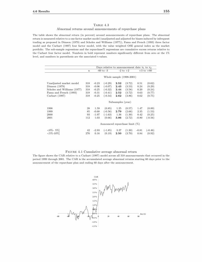
4.6 Results 155
Table 4.3Abnormal returns around announcements of repurchase plans
The table shows the abnormal return (in percent) around announcements of repurchase plans. The abnormal
return is measured relative to a one factor market model (unadjusted and adjusted for biases induced by infrequent
trading as proposed in Dimson (1979) and Scholes and Williams (1977)), Fama and French (1993) three factor
model and the Carhart (1997) four factor model, with the value weighted OSE general index as the market
portfolio. The sub-sample regressions and the repurchase% regressions are cumulative excess returns relative to
the Carhart four factor model. Numbers in bold represent numbers significantly different from zero at the 1%
level, and numbers in parenthesis are the associated t-values.
Days relative to announcement date τ1 to τ2
n -60 to -3 -2 to +2 +3 to +60
Whole sample (1998-2001)
Unadjusted market model 318 -0.23 (-0.29) 2.52 (3.72) 0.51 (0.62)Dimson (1979) 318 -0.06 (-0.07) 2.43 (3.53) 0.24 (0.29)Scholes and Williams (1977) 318 -0.25 (-0.32) 2.44 (3.58) 0.20 (0.24)Fama and French (1993) 318 -0.31 (-0.41) 2.52 (3.72) 0.63 (0.77)Carhart (1997) 318 -0.25 (-0.34) 2.62 (3.86) 0.62 (0.75)
Subsamples (year)
1998 28 1.59 (0.85) 1.25 (0.57) 1.47 (0.89)1999 85 -0.68 (-0.56) 2.79 (2.66) 2.35 (1.53)2000 93 -1.97 (-1.63) 1.36 (1.30) 0.42 (0.25)2001 112 1.03 (0.66) 3.86 (2.72) -0.80 (-0.56)
Announced repurchase limit (%)
<0%- 5%] 42 -2.93 (-1.85) 3.37 (1.30) -0.81 (-0.46)<5%-10%] 276 0.16 (0.19) 2.50 (3.70) 0.84 (0.92)
Figure 4.1 Cumulative average abnormal returnThe figure shows the CAR relative to a Carhart (1997) model across all 318 announcements that occurred in the
period 1999 through 2001. The CAR is the accumulated average abnormal returns starting 60 days prior to the
announcement of the repurchase plan and ending 60 days after the announcement.
-1.5 %
-1.0 %
-0.5 %
0.0 %
0.5 %
1.0 %
1.5 %
2.0 %
2.5 %
3.0 %
3.5 %
4.0 %
-80 -60 -40 -20 0 20 40 60 80
CAR
day (τ)

156 Chapter 4 Open Market Share Repurchases in Norway
To examine in more detail what factors are important with respect to the size ofthe announcement effect, we run the following regression with the cumulative abnormalreturn across the event window for each announcement, CARi(τ1, τ2), as the dependentvariable,
CARi(τ1, τ2) = α + β1CARi,τ1−k + β2SPRi,τ1−k + β3MCAPi,τ1−1
+ β4BMi,τ1−1 + β5PERCi,τ + DIVi,τ1−360 + QuickRatioi,τ + εi
(4.9)
where α is the intercept term, CARi,τ1−k is the cumulative abnormal return over thek days prior to the event window, SPRi,τ1−k is the average relative spread34 across thek days prior to the event window, MCAPi,τ1−1 is the natural log of the firms marketcapitalization on the last date before the event window, BMi,τ1−1 is the book to marketvalue on the last date before the event window, PERCi,τ is the size of the repurchase plan,DIVτ1−360 is a dummy variable indicating whether a firm has paid any cash dividendsduring the previous year and QuickRatioi,τ is the most recently reported quick ratio35
before the firm announces a repurchase plan.Panel A in table 4.4 shows the results from the cross sectional regression when τ1=-
2, τ2=2 and k=20, and panel B shows the correlations between the variables. As canbe seen from panel B, the average pre-event spread (SPRi,τ1−k) is strongly negativelycorrelated with market capitalization (MCAPi,τ1−1). This is because large firms gener-ally are more liquid and has lower spreads. In addition, as noted by Vermaelen (1981),small firms may have a greater degree of asymmetric information since they are lessclosely followed by analysts and the popular press. Thus, both the spread and marketcapitalization variables capture to a large degree these same characteristics. The secondhighest correlation is between the book to market (BMi,τ1
) variable and the pre-event(20 days) cumulative abnormal return, which has a significant positive correlation of0.26. To reduce the multicolinearity problem when including all these variables in theregression, we orthogonalize both the market capitalization against the relative spreadmeasure as well as the book to market variable against the pre announcement CAR(CARi,τ1−k).36 Panel C in the table shows some descriptive statistics for the indepen-dent variables. Note that the MCAPi,τ1−1 is in natural logs and that the CARi,τ1−k isnot in percentage terms.
We estimate two models. Model 1 include all variables, and in model 2 the vari-ables related to firm liquidity are omitted. The first thing to note is that the greater
34The relative spread for a security for a day, τ, is calculated as SPRτ = (askτ − bidτ)/[(askτ +
bidτ)/2], where askτ and bidτ is the best ask and bid quotes at the close of day τ.35The quick ratio is calculated as the sum of cash and deposits, total short-term financial investments
and total short-term receivables divided by total short-term debt36When estimating the regressions with the original (nonorthogonalized) variables the results are
quantitatively similar.
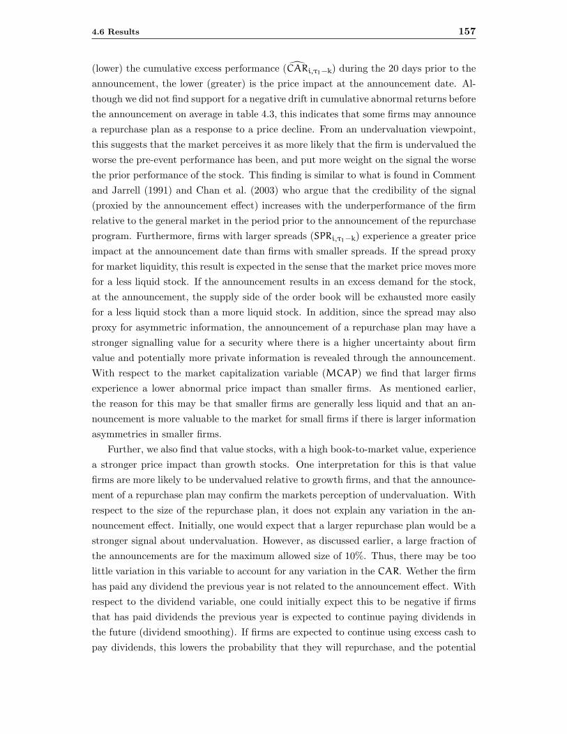
4.6 Results 157
(lower) the cumulative excess performance (CARi,τ1−k) during the 20 days prior to theannouncement, the lower (greater) is the price impact at the announcement date. Al-though we did not find support for a negative drift in cumulative abnormal returns beforethe announcement on average in table 4.3, this indicates that some firms may announcea repurchase plan as a response to a price decline. From an undervaluation viewpoint,this suggests that the market perceives it as more likely that the firm is undervalued theworse the pre-event performance has been, and put more weight on the signal the worsethe prior performance of the stock. This finding is similar to what is found in Commentand Jarrell (1991) and Chan et al. (2003) who argue that the credibility of the signal(proxied by the announcement effect) increases with the underperformance of the firmrelative to the general market in the period prior to the announcement of the repurchaseprogram. Furthermore, firms with larger spreads (SPRi,τ1−k) experience a greater priceimpact at the announcement date than firms with smaller spreads. If the spread proxyfor market liquidity, this result is expected in the sense that the market price moves morefor a less liquid stock. If the announcement results in an excess demand for the stock,at the announcement, the supply side of the order book will be exhausted more easilyfor a less liquid stock than a more liquid stock. In addition, since the spread may alsoproxy for asymmetric information, the announcement of a repurchase plan may have astronger signalling value for a security where there is a higher uncertainty about firmvalue and potentially more private information is revealed through the announcement.With respect to the market capitalization variable (MCAP) we find that larger firmsexperience a lower abnormal price impact than smaller firms. As mentioned earlier,the reason for this may be that smaller firms are generally less liquid and that an an-nouncement is more valuable to the market for small firms if there is larger informationasymmetries in smaller firms.
Further, we also find that value stocks, with a high book-to-market value, experiencea stronger price impact than growth stocks. One interpretation for this is that valuefirms are more likely to be undervalued relative to growth firms, and that the announce-ment of a repurchase plan may confirm the markets perception of undervaluation. Withrespect to the size of the repurchase plan, it does not explain any variation in the an-nouncement effect. Initially, one would expect that a larger repurchase plan would be astronger signal about undervaluation. However, as discussed earlier, a large fraction ofthe announcements are for the maximum allowed size of 10%. Thus, there may be toolittle variation in this variable to account for any variation in the CAR. Wether the firmhas paid any dividend the previous year is not related to the announcement effect. Withrespect to the dividend variable, one could initially expect this to be negative if firmsthat has paid dividends the previous year is expected to continue paying dividends inthe future (dividend smoothing). If firms are expected to continue using excess cash topay dividends, this lowers the probability that they will repurchase, and the potential
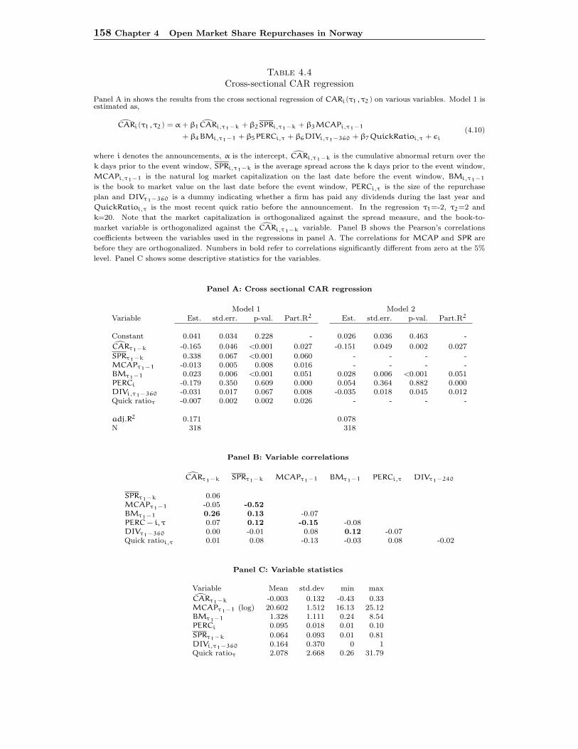
158 Chapter 4 Open Market Share Repurchases in Norway
Table 4.4Cross-sectional CAR regression
Panel A in shows the results from the cross sectional regression of CARi(τ1, τ2) on various variables. Model 1 isestimated as,
CARi(τ1, τ2) = α + β1CARi,τ1−k + β2SPRi,τ1−k + β3MCAPi,τ1−1
+ β4BMi,τ1−1 + β5PERCi,τ + β6DIVi,τ1−360 + β7QuickRatioi,τ + εi
(4.10)
where i denotes the announcements, α is the intercept, CARi,τ1−k is the cumulative abnormal return over the
k days prior to the event window, SPRi,τ1−k is the average spread across the k days prior to the event window,
MCAPi,τ1−1 is the natural log market capitalization on the last date before the event window, BMi,τ1−1
is the book to market value on the last date before the event window, PERCi,τ is the size of the repurchase
plan and DIVτ1−360 is a dummy indicating whether a firm has paid any dividends during the last year and
QuickRatioi,τ is the most recent quick ratio before the announcement. In the regression τ1=-2, τ2=2 and
k=20. Note that the market capitalization is orthogonalized against the spread measure, and the book-to-
market variable is orthogonalized against the CARi,τ1−k variable. Panel B shows the Pearson’s correlations
coefficients between the variables used in the regressions in panel A. The correlations for MCAP and SPR are
before they are orthogonalized. Numbers in bold refer to correlations significantly different from zero at the 5%
level. Panel C shows some descriptive statistics for the variables.
Panel A: Cross sectional CAR regression
Model 1 Model 2Variable Est. std.err. p-val. Part.R2 Est. std.err. p-val. Part.R2
Constant 0.041 0.034 0.228 - 0.026 0.036 0.463 -
CARτ1−k -0.165 0.046 <0.001 0.027 -0.151 0.049 0.002 0.027
SPRτ1−k 0.338 0.067 <0.001 0.060 - - - -MCAPτ1−1 -0.013 0.005 0.008 0.016 - - - -BMτ1−1 0.023 0.006 <0.001 0.051 0.028 0.006 <0.001 0.051PERCi -0.179 0.350 0.609 0.000 0.054 0.364 0.882 0.000DIVi,τ1−360 -0.031 0.017 0.067 0.008 -0.035 0.018 0.045 0.012Quick ratioτ -0.007 0.002 0.002 0.026 - - - -
adj.R2 0.171 0.078N 318 318
Panel B: Variable correlations
CARτ1−k SPRτ1−k MCAPτ1−1 BMτ1−1 PERCi,τ DIVτ1−240
SPRτ1−k 0.06MCAPτ1−1 -0.05 -0.52BMτ1−1 0.26 0.13 -0.07PERC − i, τ 0.07 0.12 -0.15 -0.08DIVτ1−360 0.00 -0.01 0.08 0.12 -0.07Quick ratioi,τ 0.01 0.08 -0.13 -0.03 0.08 -0.02
Panel C: Variable statistics
Variable Mean std.dev min max
CARτ1−k -0.003 0.132 -0.43 0.33MCAPτ1−1 (log) 20.602 1.512 16.13 25.12BMτ1−1 1.328 1.111 0.24 8.54PERCi 0.095 0.018 0.01 0.10
SPRτ1−k 0.064 0.093 0.01 0.81DIVi,τ1−360 0.164 0.370 0 1Quick ratioτ 2.078 2.668 0.26 31.79
4.6 Results 159
positive effects related to repurchases discussed in section 4.2 are less likely to occur.Finally, the most recent quick ratio before the announcement, is negatively related tothe announcement effect. Initially, one would expect this variable to be positive in thesense that liquid firms may be expected to actually execute repurchases such that thesignal is more credible when firms are liquid. On the other hand, the announcementmay to a greater extent be expected by the market in these cases.
4.6.2 Long-term performance of firms announcing a repurchase plan
In this section we examine the long term performance of firms announcing a repurchaseplan. The main hypothesis to be investigated is the underreaction hypothesis of Iken-berry et al. (1995) who argue that, if a repurchase announcement is a positive signal,this signal should be, in an efficient market, incorporated into prices completely andin an unbiased fashion when the firm announces the repurchase plan. In the previoussection we found a significant positive announcement effect of about 2.5%. In panelA of table 4.5 we report the results from evaluating the long term abnormal perfor-mance of a calendar time portfolio of announcing firms. The portfolio is rebalancedevery month. All stocks that announce a repurchase plan during a month are added tothe portfolio the first day of the following month. At the beginning of each month, allfirms receive equal weights in the portfolio. We also examine in panel B of table 4.5 theperformance of our portfolio with respect to various fixed holding periods from 1 to 4years in addition to a buy-and-hold strategy (“whole sample”) where the stock remainsin the portfolio for the rest of the period. When a stock has been in the portfolio forthe duration of the respective holding period, it is removed from the portfolio until itannounces a new repurchase plan. To reduce the idiosyncratic risk of the portfolio, werequire there to be at least 10 firms that has announced a repurchase plan before westart the portfolio.37
Panel A in table 4.5 shows that for a buy-and-hold portfolio, with no limit on theholding period, the portfolio significantly outperforms the market by about 0.9% permonth, or 11% per year, when we adjust for the Fama and French (1993) and Carhart(1997) risk factors. This is in line with results in Ikenberry et al. (1995, 2000) who findsan abnormal performance of 12.1% in the US and 7% per year in Canada respectively.Relative to the CAPM, the excess performance is almost 2% per month, or almost27% per year, illustrating the importance of adjusting the portfolio performance foradditional risk factors in addition to the market risk. When restricting the holdingperiod in panel B, we find, for the Fama/French and Carhart models, that there is asignificant excess performance when the holding period is longer than 1 year. Withrespect to a CAPM specification, the portfolio outperforms regardless of the chosen
37When we use the entire sample period, this result in our portfolio starting in October 1998, when10 firms had announced a repurchase plan.
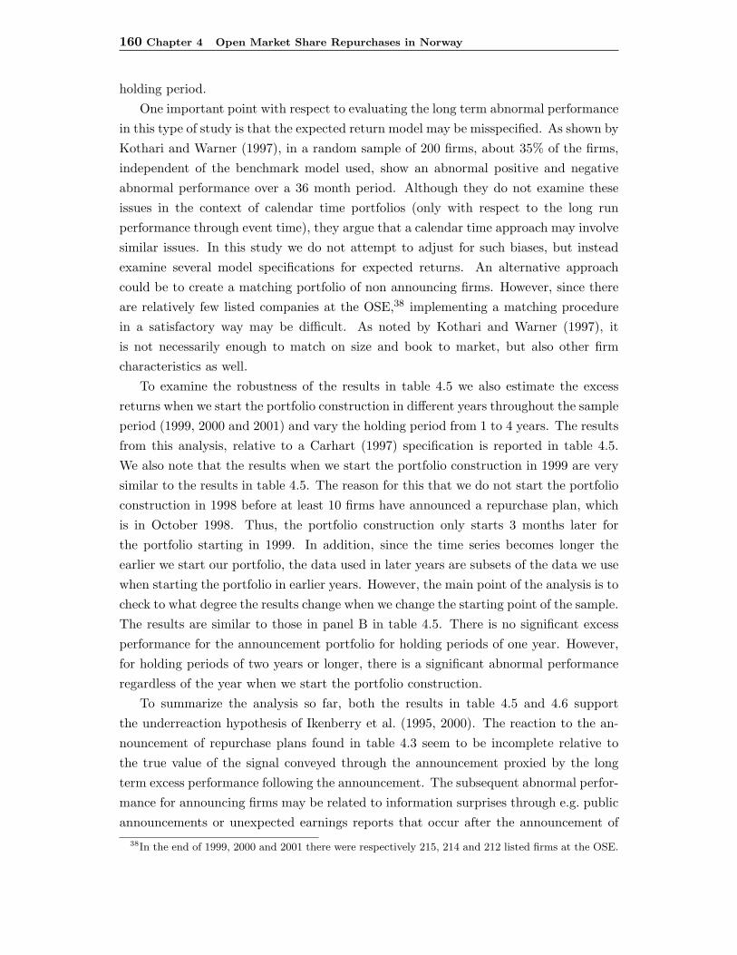
160 Chapter 4 Open Market Share Repurchases in Norway
holding period.One important point with respect to evaluating the long term abnormal performance
in this type of study is that the expected return model may be misspecified. As shown byKothari and Warner (1997), in a random sample of 200 firms, about 35% of the firms,independent of the benchmark model used, show an abnormal positive and negativeabnormal performance over a 36 month period. Although they do not examine theseissues in the context of calendar time portfolios (only with respect to the long runperformance through event time), they argue that a calendar time approach may involvesimilar issues. In this study we do not attempt to adjust for such biases, but insteadexamine several model specifications for expected returns. An alternative approachcould be to create a matching portfolio of non announcing firms. However, since thereare relatively few listed companies at the OSE,38 implementing a matching procedurein a satisfactory way may be difficult. As noted by Kothari and Warner (1997), itis not necessarily enough to match on size and book to market, but also other firmcharacteristics as well.
To examine the robustness of the results in table 4.5 we also estimate the excessreturns when we start the portfolio construction in different years throughout the sampleperiod (1999, 2000 and 2001) and vary the holding period from 1 to 4 years. The resultsfrom this analysis, relative to a Carhart (1997) specification is reported in table 4.5.We also note that the results when we start the portfolio construction in 1999 are verysimilar to the results in table 4.5. The reason for this that we do not start the portfolioconstruction in 1998 before at least 10 firms have announced a repurchase plan, whichis in October 1998. Thus, the portfolio construction only starts 3 months later forthe portfolio starting in 1999. In addition, since the time series becomes longer theearlier we start our portfolio, the data used in later years are subsets of the data we usewhen starting the portfolio in earlier years. However, the main point of the analysis is tocheck to what degree the results change when we change the starting point of the sample.The results are similar to those in panel B in table 4.5. There is no significant excessperformance for the announcement portfolio for holding periods of one year. However,for holding periods of two years or longer, there is a significant abnormal performanceregardless of the year when we start the portfolio construction.
To summarize the analysis so far, both the results in table 4.5 and 4.6 supportthe underreaction hypothesis of Ikenberry et al. (1995, 2000). The reaction to the an-nouncement of repurchase plans found in table 4.3 seem to be incomplete relative tothe true value of the signal conveyed through the announcement proxied by the longterm excess performance following the announcement. The subsequent abnormal perfor-mance for announcing firms may be related to information surprises through e.g. publicannouncements or unexpected earnings reports that occur after the announcement of
38In the end of 1999, 2000 and 2001 there were respectively 215, 214 and 212 listed firms at the OSE.
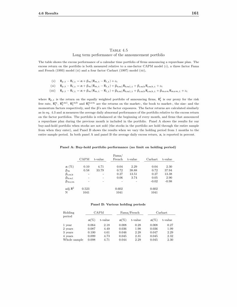
4.6 Results 161
Table 4.5Long term performance of the announcement portfolio
The table shows the excess performance of a calendar time portfolio of firms announcing a repurchase plan. The
excess return on the portfolio is both measured relative to a one-factor CAPM model (i), a three factor Fama
and French (1993) model (ii) and a four factor Carhart (1997) model (iii),
(i) Rp,t − Rf,t = α + βm(Rm,t − Rf,t) + εt
(ii) Rp,t − Rf,t = α + βm(Rm,t − Rf,t) + βhmlRhml,t + βsmbRsmb,t + εt
(iii) Rp,t − Rf,t = α + βm(Rm,t − Rf,t) + βhmlRhml,t + βsmbRsmb,t + βmomRmom,t + εt
where Rp,t is the return on the equally weighted portfolio of announcing firms, Rft is our proxy for the risk
free rate, Rmτ , Rhml
τ , Rsmbτ and Rmom
τ are the returns on the market-, the book to market-, the size- and the
momentum factors respectively, and the β’s are the factor exposures. The factor returns are calculated similarly
as in eq. 4.3 and α measures the average daily abnormal performance of the portfolio relative to the excess return
on the factor portfolios. The portfolio is rebalanced at the beginning of every month, and firms that announced
a repurchase plan during the previous month is included in the portfolio. Panel A shows the results for our
buy-and-hold portfolio when stocks are not sold (the stocks in the portfolio are hold through the entire sample
from when they enter), and Panel B shows the results when we vary the holding period from 1 months to the
entire sample period. In both panel A and panel B the average daily excess return, α, is reported in percent.
Panel A: Buy-hold portfolio performance (no limit on holding period)
Fama/CAPM t-value French t-value Carhart t-value
α (%) 0.10 4.71 0.04 2.29 0.04 2.30βm 0.58 33.79 0.72 38.88 0.72 37.94βsmb - - 0.27 13.51 0.27 13.38βhml - - 0.06 3.74 0.05 2.90βmom - - - - -0.02 -0.98
adj.R2 0.523 0.602 0.602N 1041 1041 1041
Panel B: Various holding periods
Holding CAPM Fama/French Carhartperiod
α(%) t-value α(%) t-value α(%) t-value
1 year 0.064 2.18 0.008 0.28 0.008 0.272 years 0.087 4.49 0.036 1.98 0.036 1.993 years 0.100 4.61 0.046 2.28 0.047 2.294 years 0.099 4.73 0.045 2.31 0.045 2.32Whole sample 0.098 4.71 0.044 2.29 0.045 2.30
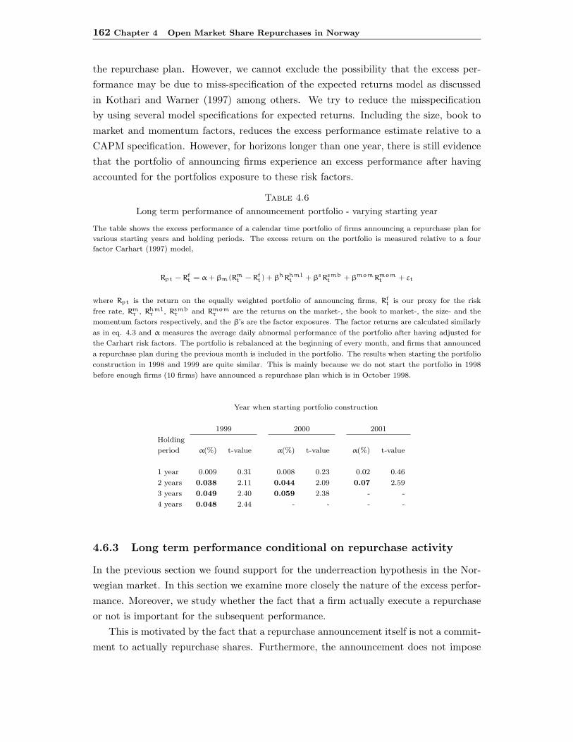
162 Chapter 4 Open Market Share Repurchases in Norway
the repurchase plan. However, we cannot exclude the possibility that the excess per-formance may be due to miss-specification of the expected returns model as discussedin Kothari and Warner (1997) among others. We try to reduce the misspecificationby using several model specifications for expected returns. Including the size, book tomarket and momentum factors, reduces the excess performance estimate relative to aCAPM specification. However, for horizons longer than one year, there is still evidencethat the portfolio of announcing firms experience an excess performance after havingaccounted for the portfolios exposure to these risk factors.
Table 4.6
Long term performance of announcement portfolio - varying starting year
The table shows the excess performance of a calendar time portfolio of firms announcing a repurchase plan for
various starting years and holding periods. The excess return on the portfolio is measured relative to a four
factor Carhart (1997) model,
Rpt − Rft = α + βm(Rm
t − Rft) + βhRhml
t + βsRsmbt + βmomRmom
t + εt
where Rpt is the return on the equally weighted portfolio of announcing firms, Rft is our proxy for the risk
free rate, Rmτ , Rhml
τ , Rsmbτ and Rmom
τ are the returns on the market-, the book to market-, the size- and the
momentum factors respectively, and the β’s are the factor exposures. The factor returns are calculated similarly
as in eq. 4.3 and α measures the average daily abnormal performance of the portfolio after having adjusted for
the Carhart risk factors. The portfolio is rebalanced at the beginning of every month, and firms that announced
a repurchase plan during the previous month is included in the portfolio. The results when starting the portfolio
construction in 1998 and 1999 are quite similar. This is mainly because we do not start the portfolio in 1998
before enough firms (10 firms) have announced a repurchase plan which is in October 1998.
Year when starting portfolio construction
1999 2000 2001
Holding
period α(%) t-value α(%) t-value α(%) t-value
1 year 0.009 0.31 0.008 0.23 0.02 0.46
2 years 0.038 2.11 0.044 2.09 0.07 2.59
3 years 0.049 2.40 0.059 2.38 - -
4 years 0.048 2.44 - - - -
4.6.3 Long term performance conditional on repurchase activity
In the previous section we found support for the underreaction hypothesis in the Nor-wegian market. In this section we examine more closely the nature of the excess perfor-mance. Moreover, we study whether the fact that a firm actually execute a repurchaseor not is important for the subsequent performance.
This is motivated by the fact that a repurchase announcement itself is not a commit-ment to actually repurchase shares. Furthermore, the announcement does not impose
4.6 Results 163
any costs on the managers in the announcing firms if the announcement is false.39 Thus,as discussed in Fried (2002) and Comment and Jarrell (1991), the credibility of the signalmay be questionable. On the other hand, when a firm actually executes a repurchase,this may be perceived as a stronger signal about undervaluation since it involves realtransactions. Especially, if the manager or other insiders owns a stake in the company,since if they repurchase when the firm is overvalued, the managers will increase theirownership in an overvalued firm (assuming that they retain their shares). Thus, whenthe market observes that the firm executes a repurchase it may be interpreted as a signal(or confirmation of the initial signal) that the the firm is actually undervalued.
Given that undervaluation is the main motivation for why firms repurchase shares,the actual repurchase executions should be a positive signal to the market about firmvalue. Moreover, one would expect the firm to execute repurchases until the firm is nolonger undervalued. If this is the case we expect the market to react positively to theactual repurchases, and increase prices closer to the true value. Furthermore, if the firmsrepurchase activity increases the price closer to the true value, reducing the mispricing,this should also reduce the subsequent long run excess performance for these firms.40
Announcements that do not result in subsequent repurchases, may be because ofseveral reasons. First of all, the firm may simply not be mispriced after the announce-ment. If these firms are more able to credibly signal that they are undervalued throughthe announcement of a repurchase plan, and the market fully reacts to the informationconveyed by the announcement, one would not expect these firms to repurchase anyshares after the announcement (at least not for undervaluation reasons). If this is thecase, we would expect announcements that do not result in subsequent repurchases toexperience a greater announcement effect than announcements that result in subsequentrepurchases. To check this, we examine, in table 4.7, whether announcements that donot result in subsequent repurchases experience a stronger announcement effect thanannouncements that result in repurchases. The results suggest that the announcementeffect (as well as the pre- and post-announcement CAR) is similar for the two groups.Thus, there is no evidence that announcements which result in subsequent repurchasesexperience a greater underreaction than announcements that do not result in repur-chases. Rather, the market reaction in the two cases are remarkably similar.
Another reason for why firms do not execute any repurchases may be because ofliquidity reasons. This can be due to low profitability or that they do not have anyexcess cash available for repurchasing shares. Thus, from an undervaluation perspective,the managers may want to repurchase shares due to undervaluation, but are unable todo so.41 An additional reason for why firms do not repurchase shares during the course
39As proposed by Fried (2002), if managers act opportunistically they may also announce a repurchaseplan when the firm is not undervalued to boost the stock price when selling.
40As discussed in section 4.2, firms also repurchase shares for many other reasons than undervaluation.However, our main discussion will be centered around the undervaluation hypothesis.
41The managers could also issue debt to finance the repurchases, but this may be costly if the firm

164 Chapter 4 Open Market Share Repurchases in Norway
Table 4.7Announcement CAR given subsequent repurchase activity
The table shows the abnormal returns (in percent) for different periods around the announcement of repurchase
programs that resulted in actual repurchases versus announcements that did not result in subsequent repurchases.
The table also show the p-value from a test that the means between the two groups are equal.
Days relative toannouncement date (τ1 to τ2)
n -60 to -3 -2 to +2 +3 to +60
Announcement, no repurchase 133 -0.05% 2.39% 0.89%Announcement, repurchase 185 -0.40% 2.78% 0.43%
Test for differencein means (p-value) 0.54 0.75 0.62
of a repurchase program is discussed in Ikenberry et al. (2000). Findings in Ikenberryet al. (2000) indicates that managers are sensitive to price movements. Thus, if theprice increases, such that the stock potentially becomes overvalued, the manager maychoose not to execute repurchases.
Our main hypothesis is that if managers execute repurchases to exploit undervalu-ation, and the market efficiently reacts to the signal conveyed through the actual re-purchases, the repurchase activity should mitigate the mispricing. Moreover, the priceshould increase towards the ”true” value if the actual repurchases signal undervaluation.This should further reduce the subsequent excess returns closer to expected levels for aportfolio of these firms. In other words, we should observe a lower subsequent abnormalperformance for repurchasing firms if the initial repurchases are successful in reducingthe mispricing. In addition, we should also see a positive, and permanent price impactfrom the actual repurchases if the market respond favorably to the information that thefirm has executed repurchases (this will be examined more closely in section 4.6.4).
Relative to what we expect to see for the group of non-repurchasing firms, this isnot clear. As discussed earlier, these firms may both choose to repurchase because theyare not mispriced which imply that these firms should perform as expected. Alterna-tively, these firms may experience a price increase after the announcement such that themanagers choose not to repurchase any shares (Ikenberry et al., 2000), in which casewe expect these firms to show an abnormal performance if the price increase is relatedto new information. Also, if these firms are undervalued after the announcement, butare unable to execute repurchases due to e.g. liquidity constraints, we would also expectthese firms to show an long run abnormal performance if prices are adjusted in responseto favorable information arrivals in later periods. On the other hand, if these firmschoose not to repurchase because they are overvalued, we would expect these firms tounderperform in the long run.
already have a high leverage ratio or that the undervaluation is to small to justify an issue of debt.
4.6 Results 165
To examine these questions in more detail, we construct a portfolio through calendartime in the similar fashion as we did when we examined the long term performance ofannouncing firms in the previous section. However, instead of only selecting our portfoliostocks conditional on whether the firm has announced a repurchase plan, we now alsocondition our stock selection on whether a firm has executed its first repurchase as well.More specifically, we create two portfolios, assigning firms based on whether they haverepurchased shares in the previous period or not. In the first portfolio (P1) we includea firm the first day of the month following the month when it announced a repurchaseplan (similar to the portfolio created in the previous section). Next, if a firm in P1executes a repurchase, we remove the firm from P1 the following day and include it ina second portfolio (P2) the first day of the following month after it for the first timehas executed a repurchase.42 Thus, P1 will at any point in time only contain firms thathave announced a repurchase plan, but not yet repurchased, while P2 contains firmsthat have executed at least one repurchase following an announcement. The combinedportfolio of the firms in P1 and P2, is the portfolio that was analyzed in section 4.6.2,such that P1 and P2 represent a decomposition of the announcement portfolio.43 Thefraction of firms actually repurchasing and the fraction of outstanding shares actuallyrepurchased among Norwegian firms is reported in table 4.1. Thus, at the end of thesample period in the scenario with no limit on the holding period, and we start theportfolio construction at the beginning of the sample, we will be left with 63 firms inP1 and 100 firms in P2 at the end of the sample period.
In table 4.8 we estimate the performance of the two portfolios relative to the CAPM,Fama and French (1993) three factor model and the Carhart (1997) four factor model.On average the portfolio of firms that has not repurchased, P1, consists of 45 firms whilethe portfolio firms that execute at least one repurchase, P2, contains on average 69firms. For diversification reasons, we do not start our portfolio construction before bothportfolios each contain at least 10 firms, which is in May 1999. Estimating Jensen’s alphawith respect to the CAPM, both portfolios show a significant abnormal performance of2% (P1) and 1.6% (P2) per month. However, relative to the Fama/French and Carhartspecifications, the results indicate that P2 does not experience an abnormal performancewhile P1 experience a significant abnormal performance of about 1.2% per month. Inother words, the portfolio tracking the portfolio of repurchasing firms (after they haveexecuted their first repurchases) perform as expected while the portfolio of firms thatannounces, but do not repurchase, experience an excess performance.
This result may indicate that actual repurchases provide useful information to the42Firms may execute several repurchases before it is included in P2. However, the potential price
effect of these repurchases will not be included in either P1 or P2. Only the effect of the first repurchasewill be included in the return of P1.
43One difference however, is that since firms are removed the day after they repurchase and notincluded in P2 before the first day of the next month, there is a window where a repurchasing firm isexcluded from both portfolios.
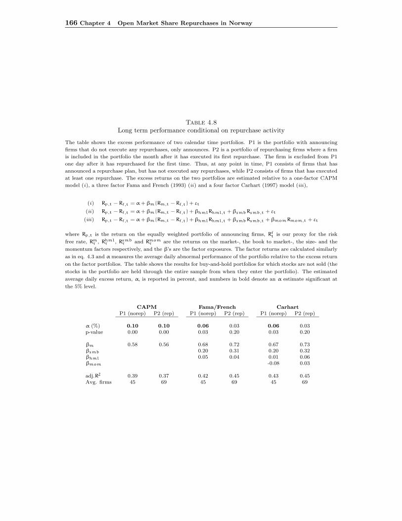
166 Chapter 4 Open Market Share Repurchases in Norway
Table 4.8Long term performance conditional on repurchase activity
The table shows the excess performance of two calendar time portfolios. P1 is the portfolio with announcing
firms that do not execute any repurchases, only announces. P2 is a portfolio of repurchasing firms where a firm
is included in the portfolio the month after it has executed its first repurchase. The firm is excluded from P1
one day after it has repurchased for the first time. Thus, at any point in time, P1 consists of firms that has
announced a repurchase plan, but has not executed any repurchases, while P2 consists of firms that has executed
at least one repurchase. The excess returns on the two portfolios are estimated relative to a one-factor CAPM
model (i), a three factor Fama and French (1993) (ii) and a four factor Carhart (1997) model (iii),
(i) Rp,t − Rf,t = α + βm(Rm,t − Rf,t) + εt
(ii) Rp,t − Rf,t = α + βm(Rm,t − Rf,t) + βhmlRhml,t + βsmbRsmb,t + εt
(iii) Rp,t − Rf,t = α + βm(Rm,t − Rf,t) + βhmlRhml,t + βsmbRsmb,t + βmomRmom,t + εt
where Rp,t is the return on the equally weighted portfolio of announcing firms, Rft is our proxy for the risk
free rate, Rmτ , Rhml
τ , Rsmbτ and Rmom
τ are the returns on the market-, the book to market-, the size- and the
momentum factors respectively, and the β’s are the factor exposures. The factor returns are calculated similarly
as in eq. 4.3 and α measures the average daily abnormal performance of the portfolio relative to the excess return
on the factor portfolios. The table shows the results for buy-and-hold portfolios for which stocks are not sold (the
stocks in the portfolio are held through the entire sample from when they enter the portfolio). The estimated
average daily excess return, α, is reported in percent, and numbers in bold denote an α estimate significant at
the 5% level.
CAPM Fama/French CarhartP1 (norep) P2 (rep) P1 (norep) P2 (rep) P1 (norep) P2 (rep)
α (%) 0.10 0.10 0.06 0.03 0.06 0.03p-value 0.00 0.00 0.03 0.20 0.03 0.20
βm 0.58 0.56 0.68 0.72 0.67 0.73βsmb 0.20 0.31 0.20 0.32βhml 0.05 0.04 0.01 0.06βmom -0.08 0.03
adj.R2 0.39 0.37 0.42 0.45 0.43 0.45Avg. firms 45 69 45 69 45 69
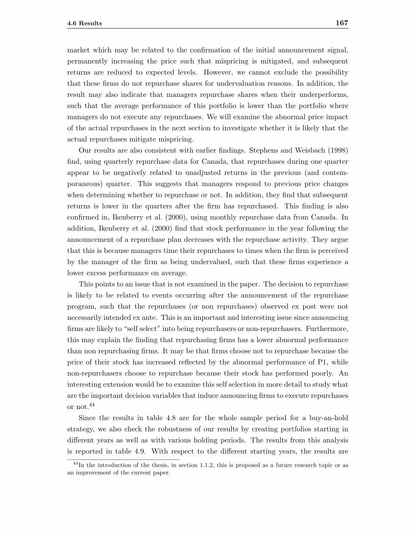
4.6 Results 167
market which may be related to the confirmation of the initial announcement signal,permanently increasing the price such that mispricing is mitigated, and subsequentreturns are reduced to expected levels. However, we cannot exclude the possibilitythat these firms do not repurchase shares for undervaluation reasons. In addition, theresult may also indicate that managers repurchase shares when their underperforms,such that the average performance of this portfolio is lower than the portfolio wheremanagers do not execute any repurchases. We will examine the abnormal price impactof the actual repurchases in the next section to investigate whether it is likely that theactual repurchases mitigate mispricing.
Our results are also consistent with earlier findings. Stephens and Weisbach (1998)find, using quarterly repurchase data for Canada, that repurchases during one quarterappear to be negatively related to unadjusted returns in the previous (and contem-poraneous) quarter. This suggests that managers respond to previous price changeswhen determining whether to repurchase or not. In addition, they find that subsequentreturns is lower in the quarters after the firm has repurchased. This finding is alsoconfirmed in, Ikenberry et al. (2000), using monthly repurchase data from Canada. Inaddition, Ikenberry et al. (2000) find that stock performance in the year following theannouncement of a repurchase plan decreases with the repurchase activity. They arguethat this is because managers time their repurchases to times when the firm is perceivedby the manager of the firm as being undervalued, such that these firms experience alower excess performance on average.
This points to an issue that is not examined in the paper. The decision to repurchaseis likely to be related to events occurring after the announcement of the repurchaseprogram, such that the repurchases (or non repurchases) observed ex post were notnecessarily intended ex ante. This is an important and interesting issue since announcingfirms are likely to “self select” into being repurchasers or non-repurchasers. Furthermore,this may explain the finding that repurchasing firms has a lower abnormal performancethan non repurchasing firms. It may be that firms choose not to repurchase because theprice of their stock has increased reflected by the abnormal performance of P1, whilenon-repurchasers choose to repurchase because their stock has performed poorly. Aninteresting extension would be to examine this self selection in more detail to study whatare the important decision variables that induce announcing firms to execute repurchasesor not.44
Since the results in table 4.8 are for the whole sample period for a buy-an-holdstrategy, we also check the robustness of our results by creating portfolios starting indifferent years as well as with various holding periods. The results from this analysisis reported in table 4.9. With respect to the different starting years, the results are
44In the introduction of the thesis, in section 1.1.2, this is proposed as a future research topic or asan improvement of the current paper.
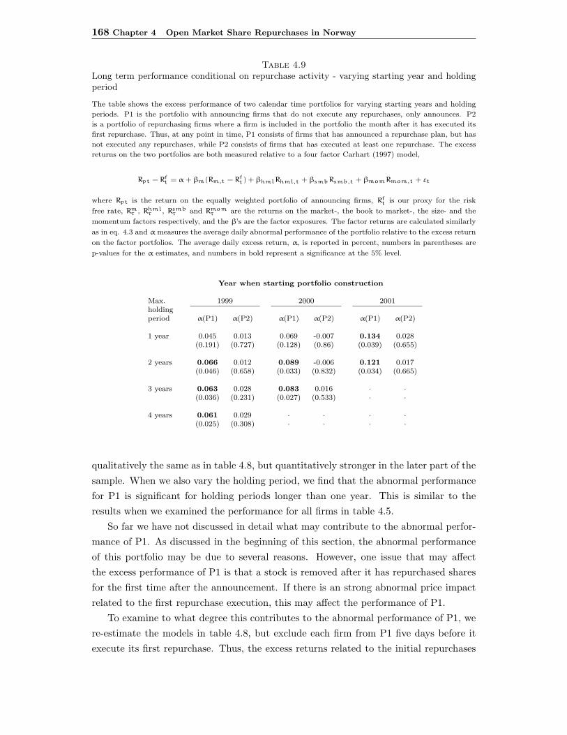
168 Chapter 4 Open Market Share Repurchases in Norway
Table 4.9Long term performance conditional on repurchase activity - varying starting year and holdingperiod
The table shows the excess performance of two calendar time portfolios for varying starting years and holding
periods. P1 is the portfolio with announcing firms that do not execute any repurchases, only announces. P2
is a portfolio of repurchasing firms where a firm is included in the portfolio the month after it has executed its
first repurchase. Thus, at any point in time, P1 consists of firms that has announced a repurchase plan, but has
not executed any repurchases, while P2 consists of firms that has executed at least one repurchase. The excess
returns on the two portfolios are both measured relative to a four factor Carhart (1997) model,
Rpt − Rft = α + βm(Rm,t − Rf
t) + βhmlRhml,t + βsmbRsmb,t + βmomRmom,t + εt
where Rpt is the return on the equally weighted portfolio of announcing firms, Rft is our proxy for the risk
free rate, Rmτ , Rhml
τ , Rsmbτ and Rmom
τ are the returns on the market-, the book to market-, the size- and the
momentum factors respectively, and the β’s are the factor exposures. The factor returns are calculated similarly
as in eq. 4.3 and α measures the average daily abnormal performance of the portfolio relative to the excess return
on the factor portfolios. The average daily excess return, α, is reported in percent, numbers in parentheses are
p-values for the α estimates, and numbers in bold represent a significance at the 5% level.
Year when starting portfolio construction
Max. 1999 2000 2001holdingperiod α(P1) α(P2) α(P1) α(P2) α(P1) α(P2)
1 year 0.045 0.013 0.069 -0.007 0.134 0.028(0.191) (0.727) (0.128) (0.86) (0.039) (0.655)
2 years 0.066 0.012 0.089 -0.006 0.121 0.017(0.046) (0.658) (0.033) (0.832) (0.034) (0.665)
3 years 0.063 0.028 0.083 0.016 · ·(0.036) (0.231) (0.027) (0.533) · ·
4 years 0.061 0.029 · · · ·(0.025) (0.308) · · · ·
qualitatively the same as in table 4.8, but quantitatively stronger in the later part of thesample. When we also vary the holding period, we find that the abnormal performancefor P1 is significant for holding periods longer than one year. This is similar to theresults when we examined the performance for all firms in table 4.5.
So far we have not discussed in detail what may contribute to the abnormal perfor-mance of P1. As discussed in the beginning of this section, the abnormal performanceof this portfolio may be due to several reasons. However, one issue that may affectthe excess performance of P1 is that a stock is removed after it has repurchased sharesfor the first time after the announcement. If there is an strong abnormal price impactrelated to the first repurchase execution, this may affect the performance of P1.
To examine to what degree this contributes to the abnormal performance of P1, were-estimate the models in table 4.8, but exclude each firm from P1 five days before itexecute its first repurchase. Thus, the excess returns related to the initial repurchases

4.6 Results 169
Table 4.10Long term performance conditional on repurchase activity - removing initial repurchase in P1
The table shows the excess performance of two calendar time portfolios. P1 is the portfolio with announcing firms
that do not execute any repurchases, only announces. To examine whether the the effect of the initial repurchase
contribute to the excess performance of P1, we exclude a firm five days before it executes its first repurchase. P2
remains identical as in the previous analysis where firms are included in the first day of the month after it has
executed its first repurchase. Thus, at any point in time, P1 consists of firms that has announced a repurchase
plan, but has not executed any repurchases, while P2 consists of firms that has executed at least one repurchase.
The excess returns on the two portfolios are both measured relative to a one-factor CAPM model (i), a three
factor Fama and French (1993) (ii) and a four factor Carhart (1997) model (iii),
(i) Rp,t − Rf,t = α + βm(Rm,t − Rf,t) + εt
(ii) Rp,t − Rf,t = α + βm(Rm,t − Rf,t) + βhmlRhml,t + βsmbRsmb,t + εt
(iii) Rp,t − Rf,t = α + βm(Rm,t − Rf,t) + βhmlRhml,t + βsmbRsmb,t + βmomRmom,t + εt
where Rp,t is the return on the equally weighted portfolio of announcing firms, Rft is our proxy for the risk
free rate, Rmτ , Rhml
τ , Rsmbτ and Rmom
τ are the returns on the market-, the book to market-, the size- and the
momentum factors respectively, and the β’s are the factor exposures. The factor returns are calculated similarly
as in eq. 4.3 and α measures the average daily abnormal performance of the portfolio relative to the excess return
on the factor portfolios. The table shows the results for buy-and-hold portfolios for which stocks are not sold (the
stocks in the portfolio are held through the entire sample from when they enter the portfolio). The estimated
average daily excess return, α, is reported in percent, and numbers in bold denote an α estimate significant at
the 5% level.
CAPM Fama/French CarhartP1 (norepo) P2 (repo) P1 (norepo) P2 (repo) P1 (norepo) P2 (repo)
α (%) 0.09 0.10 0.06 0.03 0.06 0.03p-value 0.00 0.00 0.04 0.24 0.04 0.20
βm 0.58 0.56 0.68 0.72 0.66 0.73βsmb 0.20 0.31 0.19 0.32βhml 0.05 0.04 0.01 0.06βmom -0.08 0.03
adj.R2 0.39 0.37 0.42 0.45 0.42 0.45Avg. firms 45 69 45 69 45 69
should then not be included in the performance of P1. The results from this analysis isreported in table 4.10, and it does not change the results greatly relative to the results intable 4.8. However, the estimated alpha for P1 decreases slightly, as well as its p-value,but the alpha is still significant at the 5% level for P1. Thus, the initial repurchaseseem to have an impact on the performance of P1, but it does not explain the overallabnormal performance of P1.
An alternative reason for why firms choose not to repurchase shares may be thatthe stock price increases such that the manager choose not to repurchase any shares(Ikenberry et al., 2000). This may clearly be a potential reason for why P1 experiencea long term abnormal performance. However, another explanation for why these firmsdo not execute any repurchases may be that the firms do not have any cash available torepurchase shares. Thus, if these firms experience an underreaction when they announce

170 Chapter 4 Open Market Share Repurchases in Norway
the repurchase plan, such that they are undervalued after the announcement, it maybe that they are unable to signal to the market that they are mispriced through actualrepurchases due to liquidity constraints. Moreover, given that the market underreacts tothe signal conveyed through the initial announcement, and the firm is undervalued afterthe announcement, the lack of repurchase activity keeps the price at a low level, resultingin abnormal returns when the market is faced with positive information surprises in laterperiods.
To examine more closely whether low liquidity is a likely reason for why firms donot repurchase, we examine measures of liquidity from accounting data. The liquiditymeasures we use are the most recently reported quick ratios and current ratios prior tothe announcements of the repurchase plans. The current ratio is calculated as the totalshort-term assets divided by total short-term debt, and the quick ratio is calculated asthe sum of cash and deposits, total short-term financial investments and total short-termreceivables divided by total short-term debt. In table 4.11 we examine the differencein liquidity between the firms in the two groups. The “no repurchase” group containsfirms that do not repurchase shares during the sample (the firms in portfolio P1 in theabove analysis). The first column of the table also contain the average liquidity mea-sure for all firms listed at the OSE.45 The results suggests that non-repurchasing firmsare on average significantly less liquid than repurchasing firms. Although this variessomewhat across the years, the overall difference in liquidity between non-repurchasingand repurchasing firms support a hypothesis that at least some announcing firms donot execute repurchases due to lack of liquidity. Furthermore, it also substantiates ourstory that since these firms are constrained from repurchasing, and more credibly sig-nal undervaluation, they experience a long-term abnormal drift due to e.g. informationsurprises in later periods.
To summarize, the results in this section indicates that the long term abnormalperformance experienced by firms that announce a repurchase plan, mainly is due tofirms that do not repurchase shares (P1). These results does not provide an explana-tion for the underreaction hypothesis proposed by Ikenberry et al. (1995). However,it offers an alternative interpretation in that the market rationally underreacts at theannouncement date due to the low credibility of the signal. If a firm actually executes arepurchase, this may be a stronger signal of undervaluation, such that the market priceis increased and the subsequent performance is reduced to expected levels. With respectto why the firms that do not repurchase experience a long term abnormal performance,we propose several explanations. This may be because these firms experience a priceincrease after the announcement reflected in the excess performance for this group, suchthat the manger chooses not to execute any repurchases. An additional interpretation,
45Before averaging across all the firms, we filter away the extreme observations in the upper 99%percentile. This removes 6 observations (within different years) with the largest having a quick ratio ofmore than 1000.
4.6 Results 171
Table 4.11Liquidity difference
The table shows the average liquidity of firms announcing a repurchase plan conditional on whether they execute
repurchases for the duration of the repurchase plan or not. Results are supplied for the whole sample (All years)
as well as for announcements occurring within separate years. The first column report the average across all
firms at the OSE. The proxies used to measure liquidity are the ”current ratio” calculated as total short-term
assets divided by total short-term debt, and the ”quick ratio” calculated as the sum of cash and deposits, total
short-term financial investments and total short-term receivables divided by total short-term debt. The liquidity
measure is the most recently reported by the firm before it announces the repurchase plan. We perform t-tests
for differences in means between firms that announce a repurchase plan but do not repurchase (1) and firms that
execute repurchases (2). The first test is a one sided test with the null that non-repurchasing firms has a higher
or equal liquidity to firms that repurchase. The second test is a two sided test with the null hypothesis that the
two means are equal. The p-values are adjusted conditional on whether the variance of the two distributions are
significantly different at the 5% level or not.
AllOSE firms No repurchase (1) Repurchase (2) Test for difference in means
Mean Mean Std.err N Mean Std.err N (2) <= (1) (1) = (2)p-value p-value
Quick ratio
All years 2.32 1.66 0.14 63 2.47 0.24 100 <0.01 <0.01
1998 2.48 1.97 0.38 13 1.91 0.31 15 0.54 0.911999 2.31 1.55 0.22 44 2.23 0.31 41 0.04 0.082000 2.36 1.41 0.18 25 2.88 0.43 65 <0.01 <0.012001 2.14 1.84 0.31 49 2.37 0.49 60 0.18 0.37
Current ratio
All years 2.65 1.98 0.14 63 2.72 0.23 100 <0.01 0.01
1998 2.96 2.31 0.35 13 2.10 0.29 15 0.68 0.631999 2.62 1.86 0.21 44 2.56 0.21 41 0.03 0.052000 2.63 1.74 0.22 25 3.13 0.42 65 <0.01 <0.012001 2.36 2.16 0.33 49 2.58 0.49 60 0.24 0.47
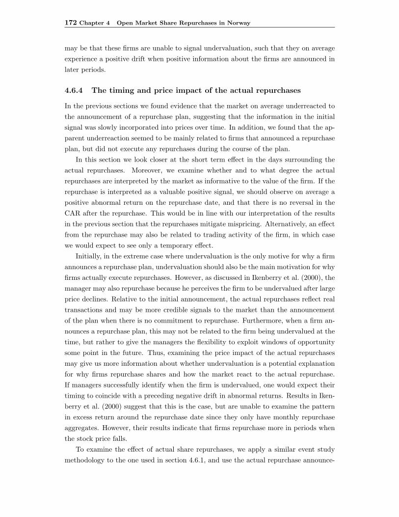
172 Chapter 4 Open Market Share Repurchases in Norway
may be that these firms are unable to signal undervaluation, such that they on averageexperience a positive drift when positive information about the firms are announced inlater periods.
4.6.4 The timing and price impact of the actual repurchases
In the previous sections we found evidence that the market on average underreacted tothe announcement of a repurchase plan, suggesting that the information in the initialsignal was slowly incorporated into prices over time. In addition, we found that the ap-parent underreaction seemed to be mainly related to firms that announced a repurchaseplan, but did not execute any repurchases during the course of the plan.
In this section we look closer at the short term effect in the days surrounding theactual repurchases. Moreover, we examine whether and to what degree the actualrepurchases are interpreted by the market as informative to the value of the firm. If therepurchase is interpreted as a valuable positive signal, we should observe on average apositive abnormal return on the repurchase date, and that there is no reversal in theCAR after the repurchase. This would be in line with our interpretation of the resultsin the previous section that the repurchases mitigate mispricing. Alternatively, an effectfrom the repurchase may also be related to trading activity of the firm, in which casewe would expect to see only a temporary effect.
Initially, in the extreme case where undervaluation is the only motive for why a firmannounces a repurchase plan, undervaluation should also be the main motivation for whyfirms actually execute repurchases. However, as discussed in Ikenberry et al. (2000), themanager may also repurchase because he perceives the firm to be undervalued after largeprice declines. Relative to the initial announcement, the actual repurchases reflect realtransactions and may be more credible signals to the market than the announcementof the plan when there is no commitment to repurchase. Furthermore, when a firm an-nounces a repurchase plan, this may not be related to the firm being undervalued at thetime, but rather to give the managers the flexibility to exploit windows of opportunitysome point in the future. Thus, examining the price impact of the actual repurchasesmay give us more information about whether undervaluation is a potential explanationfor why firms repurchase shares and how the market react to the actual repurchase.If managers successfully identify when the firm is undervalued, one would expect theirtiming to coincide with a preceding negative drift in abnormal returns. Results in Iken-berry et al. (2000) suggest that this is the case, but are unable to examine the patternin excess return around the repurchase date since they only have monthly repurchaseaggregates. However, their results indicate that firms repurchase more in periods whenthe stock price falls.
To examine the effect of actual share repurchases, we apply a similar event studymethodology to the one used in section 4.6.1, and use the actual repurchase announce-

4.6 Results 173
Figure 4.2 CAR around actual repurchases - unfilteredThe figure shows the CAR from 50 days before the actual repurchase until 50 days after the repurchase. In the
figure we average across all 1375 event dates.
-4.0 %
-3.5 %
-3.0 %
-2.5 %
-2.0 %
-1.5 %
-1.0 %
-0.5 %
0.0 %
0.5 %
1.0 %
-60 -40 -20 0 20 40 60
day (τ)
CAR
ment date as the event. This date is either the same day as the repurchase or before thetrading session starts the next day. One main problem with analyzing the actual repur-chases is that there are about 1375 repurchase events over a 4 year period. Since firmsoften repurchase shares on several days in a row, this clustering of events is problematicin several respects. First of all, if a firm execute several repurchases in sequence, theevent dates will be overlapping and dependent. This results in the post and pre-eventexcess returns being averaged across overlapping periods. Thus, if firms repurchasewhen there is a negative drift in excess returns, the average negative excess return willbe exaggerated. Figure 4.2 shows the average cumulative abnormal returns from 50days before to 50 days after the repurchase when we ignore these problems and use all1375 repurchase events. Although the numbers used in the figure are subject to severalproblems related to the clustering of events, and that firms that repurchase more gaina larger weight, it illustrates that repurchases are executed in periods when the stockexperience a downward drift in abnormal performance. In addition, there seem to be atemporary increase in the stock price around the repurchases date. Thus, the normalperformance of the repurchase portfolio (P2) in the previous section, may be becausethese firms perform worse on average than non-repurchasing firms in (P1).
To reduce the bias related to the clustering of repurchases discussed above, wecalculate short term excess returns for two main cases. First, for each firm, we restrictrepurchases to be 40 days apart to be included in the sample. Although this reducesthe bias related to overlapping, the excess returns both before and after the repurchasecontain potential abnormal price movements related to repurchases that are not included
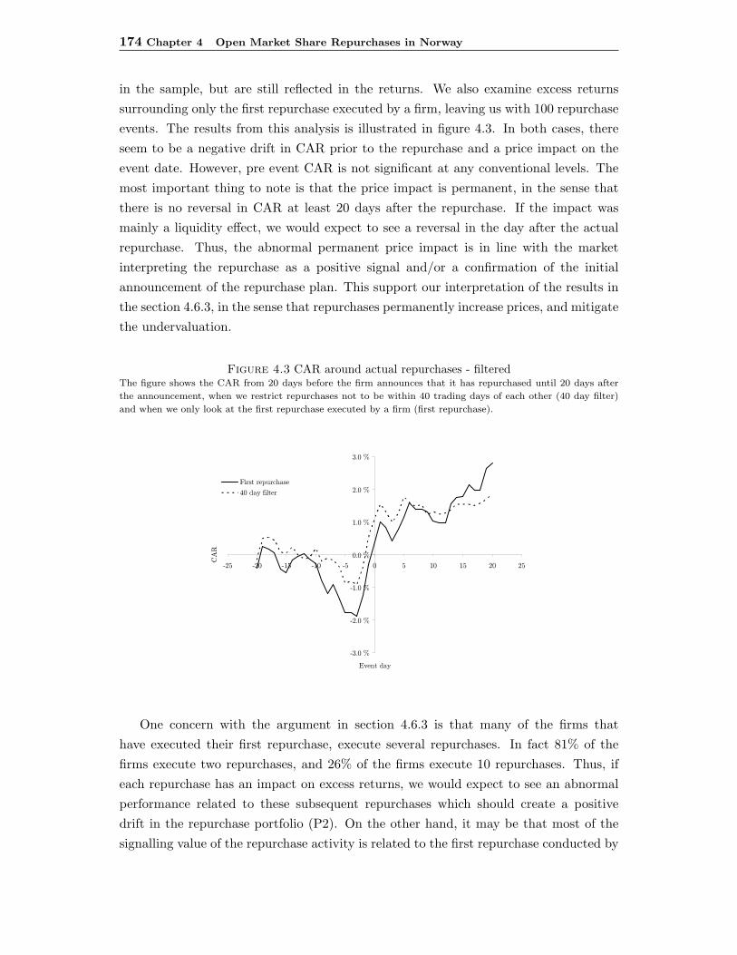
174 Chapter 4 Open Market Share Repurchases in Norway
in the sample, but are still reflected in the returns. We also examine excess returnssurrounding only the first repurchase executed by a firm, leaving us with 100 repurchaseevents. The results from this analysis is illustrated in figure 4.3. In both cases, thereseem to be a negative drift in CAR prior to the repurchase and a price impact on theevent date. However, pre event CAR is not significant at any conventional levels. Themost important thing to note is that the price impact is permanent, in the sense thatthere is no reversal in CAR at least 20 days after the repurchase. If the impact wasmainly a liquidity effect, we would expect to see a reversal in the day after the actualrepurchase. Thus, the abnormal permanent price impact is in line with the marketinterpreting the repurchase as a positive signal and/or a confirmation of the initialannouncement of the repurchase plan. This support our interpretation of the results inthe section 4.6.3, in the sense that repurchases permanently increase prices, and mitigatethe undervaluation.
Figure 4.3 CAR around actual repurchases - filteredThe figure shows the CAR from 20 days before the firm announces that it has repurchased until 20 days after
the announcement, when we restrict repurchases not to be within 40 trading days of each other (40 day filter)
and when we only look at the first repurchase executed by a firm (first repurchase).
Tn�(S0
T1�(S0
Td�(S0
(�(S0
d�(S0
1�(S0
n�(S0
T1x T1( Tdx Td( Tx ( x d( dx 1( 1x
e%�t�SIsk
]Vi
3$�R�S��}Z�{YsR�
;(SIskSP$j���
One concern with the argument in section 4.6.3 is that many of the firms thathave executed their first repurchase, execute several repurchases. In fact 81% of thefirms execute two repurchases, and 26% of the firms execute 10 repurchases. Thus, ifeach repurchase has an impact on excess returns, we would expect to see an abnormalperformance related to these subsequent repurchases which should create a positivedrift in the repurchase portfolio (P2). On the other hand, it may be that most of thesignalling value of the repurchase activity is related to the first repurchase conducted by

4.6 Results 175
a firm, since it conveys to the market that the firm is committed to actually repurchasingshares. If so, most of the price correction occurs before the stock is included in the secondportfolio (P2), such that the subsequent performance is not affected by the continuingrepurchase activity. To examine this in more detail we estimate the CAR for the threeday period surrounding the actual repurchase, from τ1=-1 (when the firm actuallyexecute the repurchase), through τ2=1 (one day after the firm has announced that ithas repurchased). We do this for each n’th repurchase event. In table 4.12 ”Repurchasenumber” denotes the sequence number of the repurchase. Thus, 100 firms executed onerepurchase, 81 firms execute a second repurchase etc. For each subsequent repurchaseevent we report the percentage CAR for the event window, the standard deviation of theCARs related to the event and the associated t-value. As opposed to the event study insection 4.6.1 where we estimated the variance for the excess returns prior to the event,we use the event window standard deviation when we examine the abnormal returnsrelated to actual repurchases. This estimator of the variance takes into account thepossibility that the event itself increases the risk of the firm, as suggested in Campbellet al. (1997). In addition, the two last columns of the table shows the average fractionthat firms repurchase during the n’th repurchase, both with respect to the total numberof shares they repurchase in the program as well as as a percentage of outstandingshares. The results in the table indicate that the first repurchase executed by firmshas the greatest price impact of about 0.88% which is highly significant. This maysuggests that the first repurchase contains the most value to the market. After the firstrepurchase there seem to be a decrease in the effect from the subsequent repurchases.
It is also interesting to note that firms on average repurchase about 38% of theirtotal repurchase amount during their first repurchase. This is also evident when lookingat the repurchase volume as a fraction of outstanding shares, with about 1.1% of thefirm shares bought back during the initial repurchase. Thus, the largest impact fromthe initial repurchase may be due to a liquidity effect. On the other hand, a largeraverage volume may also be perceived as a stronger signal in the market. From figure4.3 there is no evidence of reversal, but rather that the CAR is relatively stable in the20 days following the repurchase.
Overall it seems like the actual repurchases are greeted by the market as a positivesignal, and that the first repurchase executed by firms is perceived as the most valuablesignal.
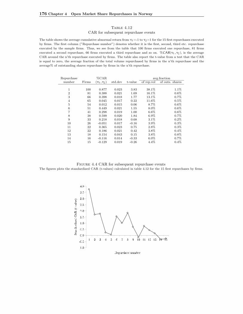
176 Chapter 4 Open Market Share Repurchases in Norway
Table 4.12CAR for subsequent repurchase events
The table shows the average cumulative abnormal return from τ1=-1 to τ2=1 for the 15 first repurchases executed
by firms. The first column (”Repurchase number”) denotes whether it is the first, second, third etc. repurchase
executed by the sample firms. Thus, we see from the table that 100 firms executed one repurchase, 81 firms
executed a second repurchase, 66 firms executed a third repurchase and so on. %CAR(τ1, τ2), is the average
CAR around the n’th repurchase executed by firms. The table also report the t-value from a test that the CAR
is equal to zero, the average fraction of the total volume repurchased by firms in the n’th repurchase and the
average% of outstanding shares repurchase by firms in the n’th repurchase.
Repurchase %CAR avg.fractionnumber Firms (τ1, τ2) std.dev t-value of rep.vol of outs. shares
1 100 0.877 0.023 3.83 38.1% 1.1%2 81 0.388 0.021 1.69 16.1% 0.6%3 66 0.398 0.018 1.77 13.1% 0.7%4 65 0.045 0.017 0.22 11.6% 0.5%5 54 0.012 0.015 0.06 8.7% 0.6%6 51 0.449 0.021 1.55 8.0% 0.6%7 41 0.298 0.019 1.00 6.6% 0.6%8 38 0.599 0.020 1.84 6.9% 0.7%9 33 0.218 0.018 0.68 3.1% 0.2%10 26 -0.051 0.017 -0.16 3.9% 0.3%11 22 0.365 0.023 0.75 2.8% 0.3%12 22 0.186 0.021 0.42 3.8% 0.4%13 18 0.154 0.043 0.15 3.8% 0.8%14 16 -0.116 0.014 -0.33 6.0% 0.7%15 15 -0.129 0.019 -0.26 4.4% 0.4%
Figure 4.4 CAR for subsequent repurchase eventsThe figures plots the standardized CAR (t-values) calculated in table 4.12 for the 15 first repurchases by firms.
� ��� �� ��� ���� ���� ���� ���� ��� ��� ��� ��� ���� �
� �����������������������������������
���! �"$#&%!'�(�) �+*�"�,.-��/#
0 1 234 254 6 7849: ;< 1 =>2? @8A
4.7 Conclusion 177
4.7 Conclusion
This paper examines a sample of announcements of repurchase plans and actual repur-chases by Norwegian firms in the period 1998 through 2001. In addition to providingevidence on open market share repurchases in a market where repurchases recently hasbeen allowed, we believe that repurchases in Norway are particularly interesting to studybecause of the legal requirement that firms report their repurchase activity on a dailybasis. By exploiting these unique data, we improve the understanding of repurchases,and how the market reacts to the actual repurchase executions.
Even during this short period, repurchases has become an important tool for Nor-wegian firms. With respect to the actual repurchase activity of Norwegian firms, wefind that about 60% of the firms that announces a repurchase plan execute at least onerepurchase during the repurchase period authorized by the shareholders. In addition,the cash distributed through repurchases as a fraction of dividends was 25% in 1999and 44% in 2000 and 2001. Furthermore, these firms repurchased on average 2.9% oftheir outstanding shares during the repurchase period.
We find support for the underreaction hypothesis investigated in Ikenberry et al.(1995) also in Norwegian data. The excess performance around the announcement ofa repurchase plan is on average about 2.5%, while a calender time portfolio of thesame firms experience a significant long term excess performance of about 0.9% permonth, or about 11% a year, relative to a Fama and French (1993) three factor modelspecification. Thus, although the market puts a positive value on the signal conveyedthrough the announcement, this indicate that it is not completely and immediatelyincorporated into prices.
In the long run, when creating two portfolios of firms that have announced a re-purchase plan and condition the portfolio construction on whether the firm actuallyexecute any repurchases, we find that the portfolio consisting only of announcing firmsthat has not yet repurchased show a significant excess performance of about 1.2% permonth. The portfolio of firms that actually execute repurchases does not experience asignificant abnormal performance. We interpret this as the market assessing the actualrepurchases as a valuable signal, increasing the stock price and aligning the subsequentlong term returns to expected levels.
For the firms that do not repurchase, we argue that their excess performance maybe related to several issues. First, it may be that these firms do not repurchase simplybecause their stock price increases after the announcement such that the manager nolonger assess the firm as being undervalued. However, an additional explanation may bethat these firms are restricted from repurchasing due to liquidity reasons. And by beingunable to signal undervaluation to the market through real transactions, their stockprice experience excess performance as the information is conveyed through positiveinformation surprises in later periods. Consistent with this interpretation we find that
178 Chapter 4 Open Market Share Repurchases in Norway
firms that do not execute any repurchases are less liquid than firms that actually executerepurchases.
When examining in more detail the timing and price impact around the actualrepurchase executions, we find that there is a negative drift in excess returns during the20 days prior to the actual repurchase. This suggests that managers execute repurchasesin periods when the stock underperforms relative to several model specifications forexpected returns. When examining the market impact of the repurchases itself, we findthat there is a significant excess return on the day when the firm execute the repurchase.In the period after the repurchase, there is no reversal in excess returns suggesting thatmarket puts a positive value on the signal that the firm has actually repurchased shares.
Overall, our findings offer additional evidence for the underreaction hypothesis.Overall, the market seem to underreact to the initial announcement. However, theabnormal performance of announcing firms is to a large degree driven by firms thatare unable to execute repurchases. If these firms are still undervalued after the an-nouncement, and unable to signal undervaluation due to liquidity constraints, the priceremains too. This result indicate that requiring repurchasing firms to announce theirrepurchases immediately may help improve price discovery.
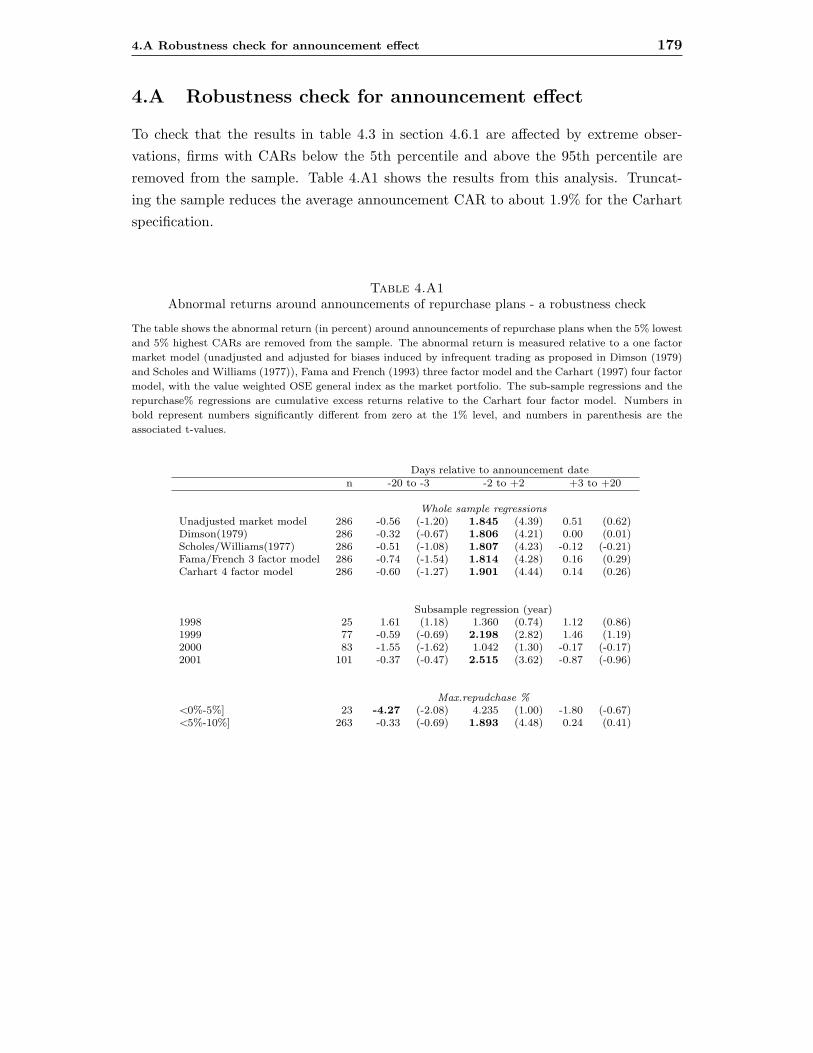
4.A Robustness check for announcement effect 179
4.A Robustness check for announcement effect
To check that the results in table 4.3 in section 4.6.1 are affected by extreme obser-vations, firms with CARs below the 5th percentile and above the 95th percentile areremoved from the sample. Table 4.A1 shows the results from this analysis. Truncat-ing the sample reduces the average announcement CAR to about 1.9% for the Carhartspecification.
Table 4.A1Abnormal returns around announcements of repurchase plans - a robustness check
The table shows the abnormal return (in percent) around announcements of repurchase plans when the 5% lowest
and 5% highest CARs are removed from the sample. The abnormal return is measured relative to a one factor
market model (unadjusted and adjusted for biases induced by infrequent trading as proposed in Dimson (1979)
and Scholes and Williams (1977)), Fama and French (1993) three factor model and the Carhart (1997) four factor
model, with the value weighted OSE general index as the market portfolio. The sub-sample regressions and the
repurchase% regressions are cumulative excess returns relative to the Carhart four factor model. Numbers in
bold represent numbers significantly different from zero at the 1% level, and numbers in parenthesis are the
associated t-values.
Days relative to announcement daten -20 to -3 -2 to +2 +3 to +20
Whole sample regressionsUnadjusted market model 286 -0.56 (-1.20) 1.845 (4.39) 0.51 (0.62)Dimson(1979) 286 -0.32 (-0.67) 1.806 (4.21) 0.00 (0.01)Scholes/Williams(1977) 286 -0.51 (-1.08) 1.807 (4.23) -0.12 (-0.21)Fama/French 3 factor model 286 -0.74 (-1.54) 1.814 (4.28) 0.16 (0.29)Carhart 4 factor model 286 -0.60 (-1.27) 1.901 (4.44) 0.14 (0.26)
Subsample regression (year)1998 25 1.61 (1.18) 1.360 (0.74) 1.12 (0.86)1999 77 -0.59 (-0.69) 2.198 (2.82) 1.46 (1.19)2000 83 -1.55 (-1.62) 1.042 (1.30) -0.17 (-0.17)2001 101 -0.37 (-0.47) 2.515 (3.62) -0.87 (-0.96)
Max.repudchase %<0%-5%] 23 -4.27 (-2.08) 4.235 (1.00) -1.80 (-0.67)<5%-10%] 263 -0.33 (-0.69) 1.893 (4.48) 0.24 (0.41)

180 Chapter 4 Open Market Share Repurchases in Norway
4.B Additional data for the sale of treasury stock
The paper only examines the gross repurchase activity by firms. However, the datasetalso contains the sale of repurchased shares (treasury stock). Table 4.B1 shows aggre-gate statistics for both repurchases as well as for the sale of treasury stock (“reverserepurchases”). The reduction in treasury stock may be due to e.g. sales of shares in theopen market, as payment in various transactions, management/employee option exer-cises, stock bonuses, stock dividends or that the treasury stock is retired. As can beseen from the table, there are almost six times as many repurchase executions as sales,and the number of repurchased shares are more than twice of what was sold. However,the size of the repurchases are on average about 1/3 of the amount that was sold. Thisindicate that firms aggregate treasury stock through many smaller repurchases, andreduce treasury stock in much larger volumes.
Table 4.B1Aggregate statistics for repurchases and sale of treasury stock
The table shows aggregate statistics for both stock repurchases as well as for “reverse” repurchases (sale of
treasury stock). The table shows the number of transactions, the total number of shares traded and the average
size of the transactions for repurchases and sales during the period from 1999 to 2002. The last part of the table
shows the fraction of buys to sales.
Size ofNumber of Shares transactions
transactions (mill.) (1000 shares)Repurchases
Whole period 1719 247.2 143.81999 205 35.3 172.22000 463 64.6 139.52001 659 107.4 163.02002 392 40.6 103.5
Sales
Whole period 293 109.4 373.51999 19 2.8 145.02000 68 26.2 385.02001 105 40.6 386.92002 101 39.9 394.9
Fraction of buys/sales
Whole period 5.87 2.26 0.381999 10.79 12.82 1.192000 6.81 2.47 0.362001 6.28 2.64 0.422002 3.88 1.02 0.26

BIBLIOGRAPHY 181
Bibliography
Allen, F. and Michaely, R. (2003). Payout Policy, in Handbooks of the Economics ofFinance, volume 1A, chapter 7, pages 337–429. Elsevier.
Bagnoli, M. and Lipman, B. I. (1989). Stock repurchases as a takeover defense. Reviewof Financial Studies, 2:423–443.
Bagwell, L. (1991). Share repurchases and takeover deterrence. RAND Journal ofEconomics, 22:72–88.
Barclay, M. J. and Smith, C. W. (1988). Corporate payout policy. Journal of FinancialEconomics, 22:61–82.
Bens, D. A., Nagar, V., and Wong, M. H. F. (2002). Real investment implications ofemployee stock option exercises. Journal of Accounting Research, 2:359–393.
Black, F. and Scholes, M. (1974). The effects of dividend yield and dividend policy oncommon stock prices and returns. Journal of Financial Economics, 1:1–22.
Brav, A., Graham, J. R., Harvey, C. R., and Michaely, R. (2003). Payout policy in the21st century. NBER Working Paper No.9657.
Brennan, M. J. and Thakor, A. V. (1990). Shareholder preferences and dividend policy.Journal of Finance, 45:993–1018.
Brockman, P. and Chung, D. Y. (2004). Managerial timing and corporate liquidity: Ev-idence from actual share repurchases. forthcoming in Journal of Financial Economics.
Brown, S. and Warner, J. (1985). Using daily stock returns: The case of event studies.Journal of Financial Economics, 14:3–31.
Brown, S. and Weinstein, M. (1985). Dervied factors in event studies. Journal ofFinancial Economics, 14:491–495.
Campbell, J., Lo, A., and MacKinlay, A. C. (1997). The Econometrics of FinancialMarkets. Princeton.
Carhart, M. (1997). Dervied factors in event studies. Journal of Finance, 52:57–82.
Chan, K., Ikenberry, D., and Lee, I. (2003). Economic sources of gain in stock repur-chases. Working Paper.
Comment, R. and Jarrell, G. A. (1991). The relative signalling power of dutch-auctionand fixed-price tender offers and open-market share repurchases. Journal of Finance,46:1243–1271.
Dann, L. Y. (1981). Common stock repurchases: An analysis of returns to bondholdersand stockholders. Journal of Financial Economics, 9:113–138.
Denis, D. J. (1990). Defensive changes in corporate payout policy: Share repurchasesand special dividends. Journal of Finance, 45:1433–1456.
182 Chapter 4 Open Market Share Repurchases in Norway
Dimson, E. (1979). Risk measurement when shares are subject to infrequent trading.Journal of Financial Economics, 7:197–226.
Dittmar, A. K. (2000). Why do firms repurchase stock? Journal of Business, 73:331–355.
Fama, E. F. and French, K. R. (1993). Common risk factors in the returns on stocksand bonds. Journal of Financial Economics, 33:3–56.
Fenn, G. W. and Liang, N. (1997). Good news and bad news about share repurchases.Working Paper, Board of Governors of the Federal Reserve, Washington D.C.
Fenn, G. W. and Liang, N. (2001). Corporate payout policy and managerial stockincentives. Journal of Financial Economics, 60:45–72.
Fried, J. M. (2002). Open market repurchases: Signaling or manegerial opportunism?UC Berkeley Public Law and Legal Theory Research Paper Series, no. 64.
Grullon, G. and Michaely, R. (2002). Dividends, share repurchases, and the substitutionhypothesis. Journal of Finance, 57:1649–1684.
Ikenberry, D., Lakonishok, J., and Vermaelen, T. (1995). Market underreaction to openmarket share repurchases. Journal of Financial Economics, 39:181–208.
Ikenberry, D., Lakonishok, J., and Vermaelen, T. (2000). Stock repurchases in canada:Performance and strategic trading. Journal of Finance, 55:2373–2397.
Institutional Investor (1998). The buyback track.
Isagawa, N. (2000). Open-market stock repurchase and stock price behavior when man-agement values real investment. The Financial Review, 35:95–108.
Jagannathan, M., Stephens, C. P., and Weisbach, M. S. (2000). Financial flexibility andthe choice between dividends and stock repurchases. Journal of Financial Economics,57:355–384.
Jensen, M. C. (1986). Agency costs of free cash flow, corporate finance, and takeovers.American Economic Review, 76:323–329.
Kothari, S. P. and Warner, J. B. (1997). Measuring long-horizon security performance.Journal of Financial Economics, 43:301–339.
Kracher, B. and Johnson, R. R. (1997). Repurchase announcements, lies and falsesignals. Journal of Business Ethics, 16:1677–1685.
Lasfer, M. A. (2000). The market valuation of share repurchases in europe. WorkingPaper, City University Business School.
Li, K. and McNally, W. J. (2002). The decision to repurchase, announcement returnsand insider holdings: A conditional event study. University of British Columbia,Working Paper UBCFIN01-2.
Lie, E. and Lie, H. J. (1999). The role of personal taxes in corporate descisions: Anempirical analysis of share repurchases and dividends. Journal of Financial and Quan-titative Analysis, 34:533–552.
BIBLIOGRAPHY 183
Lintner, J. (1956). Distribution of incomes of corporations among dividends, retainedearnings, and taxes. American Economic Review, 46:97–113.
Masulis, R. W. (1980). Stock repurchase by tender offer: An analysis of the causes ofcommon stock price changes. Journal of Finance, 35:305–319.
Miller, M. and Modigliani, F. (1961). Dividend policy, growth, and the valuation ofshares. The Journal of Business, 34:411–433.
Miller, M. H. and Rock, K. (1985). Dividend policy under asymmetric information.Journal of Finance, 40:1031–1051.
Opler, T. and Titman, S. (1996). The debt-equity choice: An analysis of issuing firms.Working Paper, Ohio State University.
Scholes, M. and Williams, J. (1977). Estimating betas from nonsynchronous data.Journal of Financial Economics, 5:309–327.
Stephens, C. P. and Weisbach, M. S. (1998). Actual share reacquisitions in open marketrepurchase programs. Journal of Finance, 53:313–333.
Vermaelen, T. (1981). Common stock repurchases and market signalling. Journal ofFinancial Economics, 9:139–183.
Womack, K. (1996). Do brokerage analysts’ recommendations have investment value?Journal of Finance, 51:137–167.

184
Chapter 5
Ownership Structure and Open
Market Share Repurchases
Written with Bernt Arne Ødegaard
Abstract
This paper provides an examination of the ownership structure in Norwegian firmsthat initiated repurchase programs during the period 1999 through 2001, as well asfor groups of these firms conditional on whether they actually executed repurchasesor not. By using detailed information on various ownership variables that canbe related to corporate governance mechanisms, the paper also examines whetherthe propensity for firms to announce a repurchase program during a given perioddepends on the ownership composition in these firms. Some interesting patternsare found which are consistent with models where firms with potentially the high-est agency problems use repurchases to mitigate agency costs. However, a veryhigh insider ownership in these firms also suggest that asymmetric information,shareholder expropriation and entrenchment may also be motivations for why firmsinitiate repurchase programs.
185
186 Chapter 5 Ownership Structure and Open Market Share Repurchases
5.1 Introduction
An open market share repurchase is an event where the repurchasing firm indirectlydistributes cash to some of its shareholders and gets in exchange a fraction of its out-standing equity.1 Compared to dividends, which generally are pro-rata distributions atregular points in time, an open market repurchase distributes cash to shareholders in annon-proportional fashion at varying points in time. Although a repurchase, at a generallevel, merely is an alternative mechanism for the firm to distribute cash, it also changesthe composition of assets held by the firm, the financing mix and alters the ownershipproportions of the remaining shareholders. Furthermore, a repurchase is also a moreflexible way for firms to distribute excess cash if they have volatile cash streams andaim at smoothing their dividends.
Although there is a large amount of research aimed at explaining the price effectof repurchase announcements and why firms choose to initiate a repurchase plan, thereare few studies that explicitly examine the relationship between ownership structureand share repurchases. This despite the fact that the initiation of a repurchase plan isan important corporate event that in some cases can alter the ownership compositionsignificantly and in the long run potentially affect the value of a firm through corporategovernance mechanisms. The ownership composition in a firm may also be an importantmotivation for firms to initiate a repurchase plan in the first place. As suggested byJensen (1986) a repurchase can help reduce the probability of incurring agency costsrelated to free cash.2 Thus, in firms with potentially severe agency problems, repur-chases may be a way for managers to convey to the market that they are committedto distribute excess cash back to the owners.3 A repurchase may also help improve thegovernance of the firm through other mechanisms as well. For example, in firms wherethere is insufficient monitoring of management,4 a repurchase may change the owner-ship composition such that the incentives to monitor management becomes greater forsome shareholders if their proportional cash-flow rights and voting rights increases. Asnoted by Shleifer and Vishny (1986), open market share repurchases are not equivalentto dividends, because they may change the share of the firm held by the large share-holder which has greater incentives to monitor. At the same time, a repurchase mayalso increase the manager’s ownership proportion in the firm such that there is a con-
1The shares owned by the company is accounted for as Treasury shares and has no cash-flow or votingrights attached to them. These shares can later be removed to decrease the shares in the company, soldback to the market, used in acquisitions, distributed to employees as a part of a bonus plan etc.
2Jensen (1986) defines free cash as the remaining cash within the firm after all projects with positivenet present values have been funded. Other suggested mechanisms for reducing agency costs of freecash is also new debt and dividends.
3This reasoning assumes that the managers actually have incentives to impose a disciplinary mech-anism on themselves.
4One example could be liquid firms with few investment opportunities, dispersed ownership andwhere management has a low stake in the firm.

5.1 Introduction 187
vergence of interest between the inside and outside shareholders (Jensen and Meckling,1976). On the other hand, a repurchase may also intensify the conflict between largeshareholders and minority shareholders. For example, if large shareholders stronger in-centives to becoming informed, a repurchase may be used to increase their ownership(and the remaining shareholders ownership) in an undervalued company by retainingtheir shares, or alternatively decrease their ownership in a overvalued company at theexpense of less informed owners (Brennan and Thakor, 1990). A repurchase may alsocontribute to the conflict between inside- and outside owners since insiders have incen-tives to secure their position in the firm. By repurchasing shares from the owners withthe lowest valuations (Bagwell, 1991) they increase the cost to a bidding firm. Thus, arepurchase can be used to reduce the probability of a value creating takeover occurring,which would benefit shareholders, but potentially make the manager loose control overthe firms resources. Also, certain types of owners may prefer one type of payout policyto another for tax reasons. For example certain investors such as pension funds andnon-profit organizations are in many countries exempt from taxes on dividends and cap-ital gains, while other investors are not. Thus, if dividends and capital gains are taxeddifferently, firms may attract different types of investors through their payout policy.Grullon and Michaely (2002) suggest that one reason for the growth in repurchases inthe US, is due to relative tax disadvantage of dividends. On the other hand, findingsin Brav et al. (2003) indicate that taxes are, at best, of second order importance whenfirms choose whether to repurchase or not.
The main focus of this paper is to investigate these issues in more detail, and toexamine whether firms that initiate repurchase programs5 have any systematic patternsin ownership that may be related to theory. In this respect, the paper has severalobjectives. The first objective is to provide a descriptive analysis of the ownershipstructure of firms that announce repurchase plans, as well as for subgroups of thesefirms conditional on whether they actually execute repurchases or not. The secondobjective is to examine whether and how the ownership changes over time in firms thatactually execute repurchases. The third objective is to study whether the propensity forfirms to initiate a repurchase program may be motivated by ownership characteristicsprior to the event.
Recent studies indicate that repurchases has become an increasingly importantmeans for firms to distribute cash. In a study on repurchase activity in the US, Grullonand Michaely (2002) find that firms gradually have substituted repurchases for divi-dends during the period from 1980 through 2000, and that US firms in 2000 spent asmuch money on repurchases as on cash dividends.6 This is also in line with findings in
5With “initiate” we mean that the firm announces a repurchase plan, which has received a super-majority vote at the general shareholder meeting. This gives the managers of the firm the opportunityto repurchase shares when they see fit over a pre-specified period. The maximum legal length of thisperiod in Norway is 18 months, but the firm is not committed to repurchase any shares.
6Grullon and Michaely (2002) find that dividend payouts grew at an annual rate of 6.8% during the

188 Chapter 5 Ownership Structure and Open Market Share Repurchases
Fama and French (2001) who find that the number of dividend paying firms has fallendramatically since 1980 until today. Similarly, in Norway, there has been an increasein spending on share repurchases, although for a much shorter time period. Since Nor-wegian firms for the first time were allowed to repurchase shares in 1999, they haveincreased their spending on repurchases as a percentage of cash dividends starting at25% in 1999 and increased this to 44% in 2000 and 2001. During the same time period,there has been a growth in aggregate dividends as well.
At a general level, a share repurchase is essentially a dividend payment, and thusan alternative way for a firm to distribute excess cash back to its shareholders. Ina world where markets are perfect and complete, whether a firm distributes its cashthrough dividends or repurchases should be equivalent according to the propositions inMiller and Modigliani (1961). Given the firms investment policy, no rational investorhas a preference for either payout policy, and through arbitrage arguments the choiceof payout policy is shown to be irrelevant with respect to the value of the firm. Onthe other hand, empirical results suggest that the information inherent in repurchaseannouncements have some economical benefits to shareholders in the sense that thesefirms on average experience an abnormal price increase when they announce that theyare planning on repurchasing shares. Among others, Vermaelen (1981), Dann (1981),Comment and Jarrell (1991), Stephens and Weisbach (1998) and Ikenberry et al. (1995,2000), find strong support for a positive announcement effect, and that this effect isabout 2%.7 These findings are comparable to what has been found with respect tounexpected dividend initiations/increases and dividend omissions/decreases (Asquithand Mullins, 1983; Michaely et al., 1995).
The dominating theoretical explanation for both of these announcement effects restson a signalling framework, in which there is asymmetric information between the man-agers and outside investors, and the announcement communicates valuable informationabout current earnings and the future prospects of the firm. As shown in Miller andRock (1985), if there is asymmetric information between investors and the managers ofa firm, changes in dividends can result in revaluations. Similarly for repurchases, modelsby Vermaelen (1981), Ofer and Thakor (1987), Constantinides and Grundy (1989), Mc-Nally (1999) and others, show that a repurchase announcement may be a valuable signalto investors about current undervaluation and the future prospects of the firm, which
period 1980 to 2000, while cash used on share repurchases grew at an annual rate of 26.1% during thesame period. From 1980 to 2000 share repurchases as a percentage of dividends increased from 13.1%in 1980 to 113.1% in 2000.
7Comment and Jarrell (1991) and Ikenberry et al. (1995) find an announcement effect in the US of2.3% (for the period 1985-1988) and 3.5% (1980-1990) respectively. In addition Comment and Jarrell(1991) examine Dutch auction repurchases and tender offer repurchases, which have a 11% and 8%price impact respectively. They argue that tender offer repurchases have the strongest signalling abilityof the three. For Canada, Li and McNally (2002) find a announcement effect of 0.9% (for the period1995-1999). Lasfer (2000) find the effect to be 1.64% in the UK, 1% for continental Europe, 0.78% inFrance and 0.63% for Italy over the period 1985 to 1998.

5.1 Introduction 189
should command a higher stock price. In addition to the signalling hypothesis, othersuggested reasons for why firms repurchase shares include, capital structure adjustments(Vermaelen, 1981; Opler and Titman, 1996), disgorgement of excess cash (Jensen, 1986;Stephens and Weisbach, 1998; Jagannathan et al., 2000), substitution for cash dividends(Grullon and Michaely, 2002), takeover defense (Denis, 1990; Bagwell, 1991; Dittmar,2000), shareholder expropriation (Brennan and Thakor, 1990), to counter the dilutioneffects of employee and management options (Fenn and Liang, 1997), personal taxes(Masulis, 1980; Lie and Lie, 1999; Grullon and Michaely, 2002) and manipulating EPSfigures (Bens et al., 2002).
With respect to the topic in this paper, the amount of research that examine the rela-tionship between ownership structure and share repurchases is much more scarce. How-ever, some exceptions include Ginglinger and L’Her (2002) who examine the relationshipbetween ownership structure and the announcement effect for French firms, Howe et al.(2003) who examine the relation between insider ownership and the announcement effectof various cash distributions in the US, including tender offer repurchases, and Li andMcNally (2002) who examine the insider holdings of repurchasing firms. The results inGinglinger and L’Her (2002) suggests that the announcement effect of controlled firms isstronger than for widely held firms, that the presence of foreign institutional investorsyield a more positive reaction and that family controlled firms experience a negativeprice effect when a repurchase program is announced. They also find that firms witha low likelihood of takeover and low risk of minority shareholder expropriation experi-ence a stronger positive announcement effect, and that the effect is highly unfavorablewhen the market participants interpret the repurchase as a takeover defense.8 Howeet al. (2003) find that there is a positive relationship between the excess return aroundvarious cash distribution events9 and the insider ownership for a sample of US firms.Their overall conclusion is that when managers owns a larger stake in the firm, theirwealth depends stronger on the success of corporate decisions and strategy such thatthe signals conveyed through payout announcements becomes more valuable/credible infirms where the inside ownership is large. Li and McNally (2002) also study the insiderholdings of repurchasing firms and find that insiders have a larger stake in firms thatinitiate repurchase plans, and that these firms experience a greater announcement effect.Their main argument for this is that insiders use repurchases to signal that they arecommitted to distribute excess cash back to the shareholders. In addition, Denis (1990)examines the price effect of defensive changes in corporate payout policy and how theownership changes in firms that remain independent after the takeover contest. Theresults indicate that these firms experience large structural changes after the takeover
8Ginglinger and L’Her (2002) proxy potential target firms as firms where the largest shareholderowns 20% of the voting rights and the float is higher than 50%.
9The cash distributions they examine are dividend increases and decreases, dividend initiations andtender offer repurchases.
190 Chapter 5 Ownership Structure and Open Market Share Repurchases
attempt in which there are large changes in capital- and ownership structure in additionto a high turnover rate among top management. Finally, Grinstein and Michaely (2001)examine the effect of institutional ownership on the choice of payout policy among firms.Their main finding is that institutions increase their ownership in firms that repurchase,but that they do not actively affect firms payout policy or cause firms to increase theiroverall payout.
There are also earlier studies on the ownership structure of Norwegian firms that areimportant to mention. Bøhren and Ødegaard (2000, 2004) provide a detailed descriptionof the ownership structure of Norwegian firms listed on the Oslo Stock exchange for theperiod 1989-1997. In addition, using the same dataset, Bøhren and Ødegaard (2001)examine whether ownership structure matters for economic performance. Their mainfindings are that insider ownership enhances firm value while ownership concentrationis negatively related to firm value.10 They also point to Norway being an atypical caserelative to the ownership structure in other countries in Europe due to very high stateownership as well as relatively high foreign ownership (about 30%). In addition, theownership by personal investors is found to be the smallest compared to any Europeancountry, and the largest shareholder owns much less while the second and third largestowner has a relatively high stake indicating that the power structure is very flat.
The analysis in this paper uses similar ownership data as used in Bøhren and Øde-gaard (2000, 2001, 2004), but for a more recent period and with monthly share-holdingsof all shareholders in all public Norwegian firms listed on the Oslo Stock Exchange(OSE). The paper combines this dataset with a sample of repurchase announcements andactual repurchases conducted by Norwegian firms for the period 1999 through 2001.11
There are several things to note about the dataset. First of all, there are few papersthat examine the actual repurchase activity of announcing firms. One reason for thisis that a large amount of studies on open market repurchases has been for US data.Due to the loose disclosure rules in the US, where firms are not required to disclose theactual repurchase executions, this has made it difficult to obtain detailed data on actualrepurchases in the US.12 By combining the repurchase dataset with a detailed ownershipdatabase containing the monthly equity holdings of all shareholders in all listed Norwe-gian firms, we are able to study in detail the ownership characteristics of these firms.In addition, we are able to examine to what degree the composition changes during therepurchase program and whether ownership characteristics affect firms propensity to
10While their results are robust in single-equation models, the relationships are rendered insignificantwhen they apply simultaneous equations models taking into account the causalities between governanceand performance.
11The repurchase sample starts in 1999 because Norwegian firms were not allowed to repurchase sharesearlier. However, firms were allowed to announce repurchase plans prior to 1999.
12One exception is Stephens and Weisbach (1998) who estimate the actual repurchase activity by USfirms based on the change in outstanding shares. In addition, during the last few years, studies onactual repurchase activity outside the US has emerged for markets where firms are subject to stricterdisclosure rules, such as Canada.
5.1 Introduction 191
initiate such programs.To summarize our main findings, we find that firms that announce at least one
repurchase program during our sample period, have a significantly lower ownershipconcentration (both when concentration is measured as the aggregate ownership of thefive largest owners and by the Herfindahl index) than firms that do not announce arepurchase plan. With respect to the number of owners, announcing firms have abouttwice as many owners as non-announcing firms, while the average size of these firmsare similar. This is in line with a story in which firms with dispersed ownership has astronger incentive to disgorge cash to mitigate agency costs related to free cash. On theother hand, our results also suggest that insiders own on average a significantly higherfraction (20%) in announcing firms than in non-announcing firms (8%), and that thisdifference is most pronounced in firms that actually repurchase shares. This, however,is not consistent with a monitoring story for repurchases, since agency theory predictsthat the insider and outsider interests are better aligned in these firms. Moreover, therewould be a lesser need for additional mechanisms to avoid agency costs of free cash inthese firms.
This finding would instead be more in line with models where insiders have incentivesto initiate a repurchase program either to maximize the future value of their personalwealth (Isagawa, 2000), expropriate outside shareholders or to entrench themselves.Moreover, Isagawa (2000) argue that if managers have stock options or ownership inthe firm, the managers objective function depends on the stock price as he gets a mon-etary compensation based on the future value of the firm. By repurchasing, this reflectsthat the manager has no profitable projects to invest in, and that his private benefitsfrom increasing the value of the firm outweighs the personal benefit from investing innegative net present value projects, which would depress the stock price in the long runand reduce his wealth. Thus, Isagawa (2000) propose an explanation for the announce-ment effect which resolves the credibility issues, in addition to offering a prediction thatrepurchasing firms have a high insider ownership. Our finding may also be consistentwith an mispricing story where there in asymmetric information between the inside- andthe outside shareholders as suggested in models by Barclay and Smith (1988) as well asBrennan and Thakor (1990) when large shareholders are better informed than smallershareholders. From this point of view, the insiders may use repurchases to transferwealth from selling shareholders to themselves (and remaining shareholders) by retain-ing their shares when the firm repurchase. Our results also indicate that the dividendpayments of announcing firms are lower than for non-announcing firms, which is con-sistent with a hypothesis where firms substitute repurchases for dividends (Grullon andMichaely, 2002). When examining the changes in ownership variables during the periodswhen firms repurchase shares the results confirm that the concentration increases. How-ever, although there is an increase in the insider ownership, it is not significant. With

192 Chapter 5 Ownership Structure and Open Market Share Repurchases
respect to the different ownertypes, the results further indicate that the ownership byinstitutions and individuals falls, while the state ownership increases. Interestingly, thisis opposite from what Grinstein and Michaely (2001) find for institutional investors inthe US. Grinstein and Michaely (2001) argue their results are inconsistent with modelsin which firms use dividends to attract institutional investors. Our results may indicatean opposite effect for Norway.
In the second part of the paper, we estimate binary models for the probability ofobserving a firm announcing a repurchase plan during each sample year given the own-ership characteristic at the beginning of the year. The results from these estimationsreflect to a great degree the findings in the descriptive part of the analysis, but providesome additional results. With respect to the insider ownership, we find that the propen-sity to initiate a repurchase program increases with insider ownership. This is in linewith findings in Li and McNally (2002) for Canada. In addition, while ownership concen-tration seem to be unimportant, a large controlling shareholder reduces the propensityfor firms to initiate a repurchase program. This is the opposite of what is the predic-tion in the model by Brennan and Thakor (1990). One implication from their modelis that large shareholders will prefer repurchases to dividends, while small shareholderswill prefer dividends. Our findings instead suggests that a controlling shareholder op-poses the initiation of a repurchase program. Alternatively, it may also reflect a lowerneed for additional mechanisms to mitigate agency costs of free cash when there is alarge shareholder in place with sufficient incentives to monitor the management. Wealso examine whether the identity13 of the largest shareholder is important, but find nosystematic evidence. The estimation results also provide evidence that firms that paiddividends in the previous year have a lower propensity to initiate a repurchase plan.This is likely related to dividend smoothing, and that firms are reluctant to cuttingdividends as suggested by findings in Lintner (1956) and Brav et al. (2003).
The remainder of the paper is structured as follows. In the next section we discusstheoretical and empirical results that motivate why there could be a relationship betweenownership structure and firms choice of repurchasing. Then we give an overview of therepurchase methods and history of repurchases in Norway, the Norwegian tax system aswell as some information about the corporate legal environment in Norway. In section5.4 we discuss the datasets and provide some general statistics, before we in in section5.5 and section 5.6 present and discuss our results and conclude in section 5.7.
5.2 Ownership structure and repurchases
In this section, we try to motivate why there could be a relationship between ownershipstructure and the choice by firms to initiate a repurchase program. Although the main
13We have information on five types of owners. These are “state” owners, “foreigners”, “financial”,“non-financial” and “individuals”.
5.2 Ownership structure and repurchases 193
purpose of the paper is to provide a descriptive analysis of repurchasing firms, it isnecessary to have a theoretical framework in which we can interpret the results andguide the analysis as well to motivate various variables used when we estimate a modelfor the propensity for firms to announce a repurchase plan. However, as discussed inBøhren and Ødegaard (2000, 2001) corporate governance has still an underdevelopedtheoretical foundation. This also affect the present paper in the sense that there arefew models directly relating firms choice of repurchases to ownership structure andcorporate governance. In other words, there are few models with clear predictions withrespect to what patterns we should expect to see. Due to the lack of a testable theory,the discussion of the results will to a large degree be partial. However, some modelsprovide implicit theoretical prediction for the relationship between ownership structure,corporate governance mechanisms and stock repurchases which we will discuss below.At a general level, it is useful to distinguish between agency- and signalling modelsused in the literature to explain why firms repurchase shares and experience a positiveannouncement effect. In the agency models, the principal (shareholder) wants to ensurethat the agent (manager) do not waste internal resources to benefit themselves. Inthese models, repurchases may be used as a mechanism to discipline the manager andreduce the cash available to him. The agency explanations however require that theshareholders can force the manager to actually repurchase or that the manager hasincentives to do so. Also, if large shareholders or insiders own a large stake in the firm,it may be difficult to initiate a repurchase plan in the first place, since it in most casesrequires a supermajority vote which can be blocked by a large shareholder. In addition,to ensure that the manager actually execute repurchases when there are no profitableinvestment opportunities may require excessive monitoring. As discussed by Jensen andMeckling (1976), it is generally impossible for the principal to costlessly ensure that theagent will act optimally from the principals viewpoint. Thus, even though a repurchaseis a cash distribution mechanism that initially could help reduce agency costs, it may notbe very effective unless the manager has incentives to disgorge free cash. In the signallingmodels, the manager may use repurchases to signal that they are committed to notwasting cash, or to convey information to the market about their private information.However, as will be discussed below, the credibility of the signal is not always clear, sincethe costs to the manager for signalling falsely may be questionable. This is especiallyimportant with respect to open market share repurchases.
Free cash flow
Agency theory predicts that non-owner managers will tend to divert parts of the firm’sfree cash flow to value-destroying projects that provide private benefits to themselves.14
14As discussed by Shleifer and Vishny (1997) such diversion by insiders may be theft, dilution ofoutside investors through share issues to insiders, salary increases, below market value share issues to

194 Chapter 5 Ownership Structure and Open Market Share Repurchases
More specifically, as discussed by Jensen and Meckling (1976), if there is low or zeroinsider ownership, and consequently a separation of ownership from control, there maybe a need for monitoring by outside shareholders to avoid that management uses internalresources in a fashion that does not maximize firm value.15 However, active monitoringby outside owners may not occur if there are no outside owners with strong incentivesto monitor the management.
In those cases payout policy is a mechanism that may help to mitigate agency costsrelated to cash. As suggested by Easterbrook (1984) and Jensen (1986) a firm may usecash distributions to reduce the agency cost of free cash by reducing the amount of cashavailable to the manager. Agency theory predicts that both debt financing, repurchasesand dividend payments are mechanisms that help mitigating agency costs. With debtfinancing, the cash flow of the firm must be used to pay creditors which potentiallycould force a bankruptcy if not paid. Dividend payments are also a way for the firm todistribute excess cash that could potentially be miss-allocated by management. The useof repurchases is potentially less costly to the firm than using dividends for distributingnon-sustainable excess cash. As proposed by Lintner (1956), managers prefer to increasedividends regularly and avoid cutting dividends if possible.16 Substantiating the findingin Lintner (1956), 94% of the company executives interviewed in Brav et al. (2003),state that they strongly try to avoid dividend cuts, and 65% answered that they wouldraise external funds before they would cut dividends. This suggest that managers viewdividend cuts as costly. One reason for this is that dividend decreases generally arepunished by the market as found in Denis et al. (1994) among others.17 Thus, firmsmay be reluctant to increasing dividends if the cash-flow is non-sustainable. In addition,studies suggests that firms aim at a target ratio and tries to smooth dividends. Thus,an unexpected dividend increase may be a stronger signal about permanent futureearnings, while a repurchase announcement may convey to the market that managementis committed to not wasting temporary cash on private benefits and value destroyingactivities.
With respect to the relationship between repurchases and ownership structure, a firmwith plenty of cash, few investment opportunities, low insider ownership and dispersedoutside ownership may benefit from using repurchases in distributing excess cash tomitigate agency costs. This in the sense that a repurchase announcement could be asignal to the market from the primary insiders that they are committed to not wasting
insiders etc.15A crucial assumption with respect to outside monitoring is that outside shareholders are competent
and that their monitoring in fact improve the quality of managerial decisions.16These arguments predict that dividend increases will be made by firms with higher and more stable
cash flows, that dividend increases will be related to permanent but not necessarily to temporary com-ponents of cash flow, and that dividend decreases will be less frequent than increases and accompaniedby very poor performance.
17Some proposed explanations for this has been signalling, overinvestment and dividend clienteles.
5.2 Ownership structure and repurchases 195
excess cash. Overall, from an agency perspective, if repurchases are motivated by poormonitoring, we would expect to see more dispersed ownership and lower ownershipconcentration in firms that announce repurchase plans. In addition, one would alsoexpect to see a lower insider ownership in these firms, since high insider ownershipinitially would reduce the need for monitoring. On the other hand, for the managers tosupport the initiation of a repurchase program as a self-imposed disciplinary mechanism,the manager must have incentives to do so. In a model by Isagawa (2000), the initiationof a repurchase program is argued to be credible despite the fact that the announcementof a repurchase plan is not a commitment to actually repurchase shares. The modelby Isagawa (2000) assumes that the managers objective function depends on the stockprice, as he gets a monetary compensation based on the future price of the firm (themanager may have stock options or own a part of the firm), in addition that he hasa private benefit from growing the size of the firm. By announcing a repurchase plan,this reflects that the manager has no profitable investment opportunities, and that thecost to him for wasting internal cash is greater than returning cash to the shareholdersand increasing the value of the firm. Thus, the announcement of a repurchase planreveals information about the managers private benefits when there are no profitableinvestment opportunities available to the firm. Li and McNally (2002) find support forthis model in that insiders have a larger stake in firms that announce repurchase plans.
Empirical results in Fenn and Liang (2001), suggest that there is a negative relation-ship between management stock ownership and the amount of cash distribution. Theyfind that firms in which managers has a low ownership stake, few investment opportuni-ties (or high free cash flow) pays out more cash. These are firms that potentially have thehighest agency problem. However, although higher insider ownership is one mechanismthat align managers interests with shareholders, it is also argued that greater ownershipby institutional owners or other large shareholders may improve outside monitoring ofthe management (Shleifer and Vishny, 1986). Grinstein and Michaely (2001) investi-gate the relationship between firms payout policy and institutional ownership in theUS, for the period 1980 through 1996, and find evidence that firms attract institutionsthrough their payout policy. More specifically, their results suggests that institutionsincrease their holdings in firms that repurchase more shares, and decrease their holdingsin firms that pay more dividends. In addition, when examining the causality betweeninstitutional ownership and payout policy, their results indicate that institutions do notactively change dividend policy or repurchase policy.
The signalling/undervaluation hypothesis
The traditional signalling hypothesis with respect to repurchases proposed by Vermaelen(1981, 1984) and Dann (1981), among others, is motivated by asymmetric informationbetween the managers of a firm and the market. If the managers of the firm has su-
196 Chapter 5 Ownership Structure and Open Market Share Repurchases
perior information about the future prospect of the firm, and know that the firm isundervalued, they can initiate a repurchase plan to convey this information. Due to thenew information about future earnings, implied by the announcement, a positive priceimpact on the announcement day is expected, as prices adjusts to the new information.Since the undervaluation hypothesis supposes that the managers of the firm has supe-rior information about the true value of the firm, and that the managers successfullyannounce repurchase plans when the firm is truly undervalued, one would also expectthe insiders of the firm to have a higher ownership fraction in these firms if they areable to trade in the firms shares.18
However, there is a problematic issue related to the signalling hypothesis and theincentives of the managers of a firm discussed in Fried (2002). The signalling hypothesisimplies that managers signal only when the firm is undervalued, and thereby sacrificetheir own wealth on behalf of the shareholders.19 The proposition in Fried (2002) is thatit is more likely that managers act opportunistically, and announce repurchase plans tomaximize their own wealth. One prediction of the model is that managers announce arepurchase plan both when the firm is undervalued as well as when it is overvalued. Themain intuition behind this is that when the firm is undervalued, the manager uses theannouncement of a plan, as well as actual repurchases, to transfer wealth to themselvesand the remaining shareholders. On the other hand, when the manager want to sella large part of her shares due to overvaluation, the repurchase announcement can beused to temporarily boost the stock price. Another argument against the signallinghypothesis is that for the signal conveyed through the announcement of a repurchaseplan to be credible, there should be an explicit commitment by the managers of thefirm.20 However, for open market share repurchases, it is rarely the case that insidersof a firm explicitly states that they are going to retain their shares for the courseof the repurchase plan. Fried (2002) argue that managers could more credibly signalundervaluation by committing to retaining their shares over a period of time.
Thus, in the managerial opportunism case of Fried (2002), the prediction with re-spect to the level of insider ownership relative to non-announcing firms is not clearsince the managers may choose to announce a repurchase plan both when the firm isundervalued and overvalued. With respect to the signaling hypothesis, however, onewould expect insider ownership to be greater in announcing firms if the managers inthese firms exploit their private information.21
18Primary insiders are generally constrained from trading in company shares around major informa-tion disclosures. However, a repurchase announcement is not generally considered as an informationrelease where the firm announce fundamental information. In these cases, it is up to the firm to definea “blackout” period for the insiders in which they are not allowed to trade company shares.
19The main argument for this is that the announcement reduces the managers financial flexibility aswell as limits the potential profits that they can reap from the information.
20At least, there should be an implicit commitment in the sense that the initial signal is backed byactual repurchases at a later point in time.
21An behavioral interpretation could be that insiders have a higher ownership in announcing firms
5.2 Ownership structure and repurchases 197
Management stock options
Fenn and Liang (2001) find evidence that managers substitute repurchases for dividendsto increase the value of their stock options. More specifically, they find a strong negativerelationship between dividend payouts and management stock options and a positiverelationship between repurchase activity and stock options. Their main interpretationof this finding is that managers will have incentives to reduce dividends and increaserepurchases (or retain more cash) because the value of the managers stock options arenegatively related to expected future dividend payments. However, as noted by Fennand Liang (2001), there are alternative explanations for a positive relationship betweenshare repurchases and stock options. One explanation could be that options increasethe managers incentives to maximize the value of the firm, and therefore also increaseprofits that is distributed to the shareholders. Another explanation may be that firmsuse repurchases to counter the dilution effects of employee and management options,such that the increased repurchase activity in firms with large amounts of managementoptions is a direct result of option exercises.
With respect to how stock options relate to the ownership structure of repurchasingfirms, one might expect there to be higher insider ownership in repurchasing firms ifrepurchases are substituted for dividends to maximize stock option values. However theprediction is not clear in the sense that risk averse managers with already a stake inthe firm, through stock ownership as well as labor income, may want to reduce theirownership fraction when they are granted more options for diversification reasons.
Expropriation of minority shareholders
So far our discussion has centered around the the potential conflict between the man-agement in a firm and the outside shareholders. However, as argued by Shleifer andVishny (1997), if large controlling shareholders participate in, or is closely connectedto, the firms management,22 or have enough power to influence the decision processwithin the firm, there may also be a conflict between controlling shareholders and mi-nority shareholders. For example, large shareholders may use the resources of a firmto benefit themselves on the expense of minority shareholder. If large shareholdersare better informed than smaller shareholders, repurchases may be used by controllingshareholders to increase their ownership further (by retaining their shares) on behalfof smaller shareholders when they have favorable information about the firm. Whena firm executes repurchases in the market, the sellers are current shareholders who,unknowingly, are trading with the firm in the open market. Thus, the cash distribution
because these managers are over-optimistic with respect to their own abilities in generating value aswell as to the firms future prospects.
22Gomes and Novaes (2002) shows that the conflict between controlling shareholders and minorityshareholders may increase when the controlling shareholders also participate in the management of thefirm.

198 Chapter 5 Ownership Structure and Open Market Share Repurchases
is essentially involuntary23 in the sense that the sellers may not have wanted to sell anyshares at the current price if they had known that the firm was the buyer. If there isasymmetric information between the managers of the firm and the market place, andthe managers are able to correctly time their repurchases accordingly, the selling share-holders execute trades against an informed investor and sell shares at a price belowfair value. Thus, if large controlling shareholders has superior information about firmvalue either through their potentially closer connection to the management or throughtheir greater incentives to collect information, they are also more likely to retain theirshares relative to small shareholders when the firm actually execute repurchases due tomispricing. Brennan and Thakor (1990) develop a theory for firms choice among severalways of paying out cash to shareholders in which there is a wealth distribution fromsmall uninformed shareholders to large, better informed, shareholders. Their modelassumes that the collection of information by investors is costly, and that stock pricesdoes not reflect all information. Since large shareholders have greater incentives to be-coming informed, small shareholders may face the risk of being expropriated by largeshareholders. Thus, small uninformed shareholders has a co-ordination problem and areunable to keep their ownership fraction constant in the event when a firm repurchasesshares. Moreover, they tend to be left with a greater ownership fraction in overvaluedfirms (when insiders or larger shareholders sell), and a lower ownership fraction in un-dervalued firms (when the firm and better informed investors buy). The center of theirargument is that non-proportionate share repurchases forces shareholders to collect in-formation and incur the gathering costs or alternatively run the risk of expropriation bybetter informed investors. As a result of this, large shareholders prefer cash to be paidout through repurchases instead of dividends, while small, potentially less informed,investors prefer dividends since these are paid pro-rata and do not bear such adverseselection costs.
The model of Brennan and Thakor (1990) is also related to the hypothesis of Barclayand Smith (1988) who argue that there is a implicit cost associated with repurchases.24
Their main hypothesis is that a repurchase plan increases the adverse selection com-ponent of the spread in the market, which again may increase the cost of capital forthe firm. If this effect is large enough, firms would prefer to use dividends instead ofrepurchases. In line with their hypothesis, they find that the spread increases after thefirm has announced a repurchase plan, and decreases to its pre-announcement level afterthe repurchase plan is completed. In other words, the increased bid-ask spread capturesthe increased probability of trading with an informed investor (the firm or the insiders
23As opposed to a tender offer repurchase where the selling shareholders know beforehand that theyare selling shares back to the firm. In addition, tender offer repurchases are generally executed at apremium to the market price, while own market share repurchases are executed at the prevailing marketprice.
24Their motivation was initially to explain why firms use dividends instead of repurchases to pay outcash despite the relative tax advantage of capital gains to dividends in the US.
5.3 Regulatory and institutional aspects 199
of the firm).
Takeover defense and entrenchment
Another motivation for management to support the initiation of a repurchase plan, aswell as actually execute repurchases, is to reduce the probability of takeovers. Thisbecause a hostile takeover, if successful, could result in the manager being replaced andloose control over the firms resources. In a hostile takeover, the acquiring firm makesan offer to the shareholders of the firm. Thus, if the firms ownership is dispersed it ismore likely that the bidding firm will be able to successfully take control. Repurchasesis one25 effective measure for managers to reduce the probability that a takeover willbe successful. Stulz (1988), argues that a stock repurchase increases the proportion ofshares held by the manager and stockholders supporting him, such that it becomes moredifficult to obtain enough shares to take control of the firm. Bagwell (1991) propose amodel with heterogenous valuations among current shareholders and an upward slopingsupply curve for the company shares. Thus, by repurchasing shares at the currentmarket price, the shareholders with the lowest valuations are removed, such that amore expensive group of shareholders are left, implying that the cost of acquiring sharesis increased. Also, Bagnoli and Lipman (1989) develop a model where they assumeasymmetric information between the managers and the market. By signalling the qualityof their firm through repurchases, this convinces the current shareholders that the valueof the company is higher such that a takeover becomes more costly. However, as shownin Denis (1990), when a repurchase announcement is interpreted as a takeover defense,the announcement effect is highly unfavorable.
Thus, while managers have incentives to oppose takeovers, firms with characteristicsthat make them likely takeover candidates is expected to be more likely to announce re-purchase plans and execute repurchases. The characteristics of a takeover candidate maydepend on many factors, but generally, undervalued firms, with low managerial owner-ship and low ownership concentration (dispersed ownership) may be more likely takeovercandidates. Thus, managers in firms with these characteristics may have stronger in-centives to entrench themselves and use repurchases to increase their ownership as wellas to remove shareholders with the lowest valuations.
5.3 Regulatory and institutional aspects
5.3.1 Repurchase methods
There are mainly three methods for firms to repurchase their own shares; through tenderoffers, open market transactions or via privately negotiated transactions, also referred
25Among other things, managers can also adapt anti-takeover amendments, ”poison pills”, increasetheir ownership proportion etc. to oppose takeover attempts.
200 Chapter 5 Ownership Structure and Open Market Share Repurchases
to as Dutch auction repurchases. The two first methods are used to a larger extentthan the latter, and in the US, open market transactions are observed more frequentlythan tender offers. In fact, 90% of the cases between 1985 and 1993 were open markettransactions as discussed in Ikenberry et al. (1995) and Stephens and Weisbach (1998).However, the size of an open market share repurchase is in general of much smallermagnitude than a tender offer repurchase. In a tender offer, the reacquiring firm offersto repurchase its shares at a specific price, usually at a premium to the market price(fixed price tender offers). In an open market repurchase, on the other hand, thepurchase is executed through brokers in the open market at normal commissions rates,and no premium is paid.26 Thus, open market repurchases is the same as a sequenceof tender offer repurchases, where the bid price is the tender price. Since tender offersare generally larger in magnitude than an open market repurchases, the alternativeof trading the shares directly in the market through open market repurchases, wouldpotentially incur a price impact cost to the firm that would exceed the premium offeredthrough the tender price, making tender offers more attractive for large distributions.
5.3.2 The introduction of repurchases in Norway
The 1st of January, 1999, the Securities Act of June 13 1997 went into effect, andNorwegian firms were allowed to repurchase their own shares. The Act states that firmsare allowed to repurchase up to 10% of the outstanding shares as long as the firm’s totalequity value in excess of the firm’s own stockholdings is higher than 1 mill. NOK. Suchlimited open market repurchase programs are often referred to as ”Normal Course IssuerBids”, whereas fixed price tender offers which do not have any limit to the amount ofstock that can be repurchased is commonly called ”Substantial Issuer Bids”.
In Norway, as in the US and other countries, the most frequently observed repurchasemethod is open market repurchases executed as a part of a Normal Course Issuer Bid,simply because Substantial Issuer Bids are only observed in a few instances. In thispaper, we only examine open market shares repurchases. Furthermore, the OSE listedfirms do not have to receive approval from the exchange before initiating a repurchaseprogram. In the U.S. the same rule applies as in Norway. However, Canadian firms(see Ikenberry et al. (2000)), must receive approval from the exchange before they caninitiate a repurchase program. In Norway, as in most countries, the managers must beauthorized by the stockholders to initiate a repurchase program. Such an authorizationis effective for the time period stated in the plan, or at most 18 months which is the legallimit. After the repurchase period has expired, there must be a new vote before the firmcan continue to repurchase shares. When a firm carries out an open market transaction
26At least no direct premium is paid. As argued by Barclay and Smith (1988), the announcementof a repurchase plan may lead to increased spread in the market due to an increased adverse selectioncomponent in the spread. Thus, by announcing a repurchase plan, the firm itself may experience higherimplicit transactions costs in the primary market when it executes repurchases.
5.3 Regulatory and institutional aspects 201
announcement rules apply, i.e. the firm must inform the OSE before the trading startsthe following day. However, if the trade is considered as being informative, the generalrule is that it must be announced to the OSE immediately.
5.3.3 The corporate environment
The main laws regulating corporations in Norway are Aksjeloven (the corporate law),Verdipapirhandelsloven (the securities law) and Børsloven (Oslo Stock Exchange reg-ulations).27 With respect to the board structure, all listed firms with more than 200employees is required to have a supervisory board which elects the board. The supervi-sory board consists of 1/3 from the employees and 2/3 owners, and the board consistsby 1/3 of the employees candidates and 2/3 consists of the owners candidates. Withrespect to to open market share repurchase programs, any owner can suggest that anrepurchase program is put on the agenda for the ordinary stockholder meeting. In ad-dition, an owner, or group of owners, representing at least 5% of the cash flow rightscan force an extraordinary stockholder meeting. A repurchase program is defined asa change in the corporate charter, and requires a super-majority vote of 2/3 from thevoting shares represented at the shareholder meeting. In addition, it requires a 2/3 votefrom all shareholders (including holders of non-voting shares) to be passed. Thus, non-voting shares may be important when it comes to proposals for changing the corporatecharter. There are also a set of regulations in place to protect minority shareholders.First, any shareholder has to report to the firm and the Oslo Stock Exchange when itpasses through various thresholds.28 If a stockholder passes 40% of the voting rights ina firm, he has to give a tender offer (Mandatory Bid) to the remaining shareholders,and if he owns at least 90% of the shares he is required to buy from any shareholderthat wants to sell shares.
There are also insider trading rules that first of all restrict all insiders from tradingon firm specific information that is important for the pricing of the stock. Furthermore,primary insiders, such as board members and the management team, are restricted fromtrading around various corporate events. For example, they are not allowed to trade twomonths before the publication of annual reports. In periods when they are allowed totrade, strict disclosure rules apply as the insider must report the transaction to the OSEwithin the trading starts the next day (10 am). Primary insiders are defined as membersof the management team, board members and substitutes. The broader definition ofall insiders also include company auditors, and the primary insiders immediate families.With respect to open market share repurchases, similar disclosure rules apply, as thefirm is required to report their transactions before the market opens the next day.
27A detailed description of the regulatory environment in Norway can be found in Bøhren and Øde-gaard (2000).
28These thresholds were 10%, 20%, 33%, 50%, 67% and 90% during the sample period.
202 Chapter 5 Ownership Structure and Open Market Share Repurchases
5.3.4 The Norwegian tax system
Dividends distributed from a Norwegian tax resident public- or private limited companywere taxed fully on the investor’s hand until 1992. As a result of an extensive tax-reform in 1992, dividends became tax-exempt while the capital gains tax was set at aflat rate of 28%, both for individuals, companies and private pension funds.29 However,shareholders in firms that retain a part of their after tax earnings, may experience thatsome of the capital gains when the shares are sold reflect a price increase due to theretained earnings. To eliminate the double taxation this would imply, an adjustment ismade. The retained earnings per share is added to the cost basis (usually the purchaseprice) such that the capital gain/tax basis is reduced accordingly (RISK adjustment).30
Thus, during the period 1992 until 2001, dividends were not taxed on the investor’shand at all, and tax on capital gains linked to retained earnings was eliminated.31
The result of this was that there were essentially was no preference in the tax systembetween capital gains or regular cash distributions. However, in 2001, a personal tax ondividends was re-introduced, at a rate of 11%, while the capital gains tax and corporatetax remained at 28%. With respect to the dividend taxation, a basic deduction ofNOK 10 000 was introduced. Thus, small investors in dividend paying firms were notdirectly affected by the tax increase. However, for larger investors the total taxationon dividends increased from 28% to 35.92%, due to the double taxation of parts of theearnings. In 2002 the personal taxation of dividends was again removed. For foreigninvestors, dividends distributed from a Norwegian tax resident public or private limitedcompany to its non-resident shareholders are subject to 25% withholding tax. Taxtreaties may make the withholding tax deductible in the shareholder’s home country.Non-resident shareholders gain on a sale of shares in a Norwegian company is not subjectto any Norwegian taxation, unless the shares form part of a permanent establishmentin Norway or the seller is an individual who fulfill certain conditions that would makethe gains taxable at a rate of 28%.
With respect to the relative tax treatment of dividends and repurchases in Norway,there has been a change during our sample period from 1999 through 2001. In 1999 and2000, dividend distributions were not taxed. On the other hand repurchases where theshareholder sells shares above the tax basis is taxed at 28%. Thus, in cases where thefirm uses already taxed earnings for repurchasing shares at a price above the tax basis,the shareholder that sell shares back to the firm would experience a double taxation onthe excess capital gains. In 2001, when a dividend tax of 11% was introduced, the tax
29labor unions, non-profit organizations and public pension funds are exempt from taxation.30RISK is the acronym for ”Regulering av Inngangsverdien med Skattlagt Kapital”. Translated, it
means that there is an adjustment of the cost basis by the retained earnings after corporate tax. To beeligible to the RISK adjustment within a given year, the shareholder must have owned the shares overthe turn of the year.
31The Norwegian tax system is a full imputation system, in which a double taxation is eliminated. Inthe UK, there is a partial imputation system, while the US has a classical company tax system.

5.4 Data description and general statistics 203
differential between capital gains and dividends was reduced, favoring repurchases.32
With respect to foreign investors, they have been subject to 25% withholding tax ondividends through the entire sample period. However, since the capital gains for for-eigners is subject to the tax in the home country, the preference between dividends andrepurchases may vary between foreign investors depending on the tax treatment in theirhome country.
5.4 Data description and general statistics
The repurchase data
The sample was formed by collecting all the announcements of open market share re-purchase programs for the period 1998 through 2001. In addition, the actual repurchaseexecutions related to these announcements reported to the Oslo Stock Exchange (OSE)from January 1999 through December 2001 were collected.33 Panel A of table 5.1 showsstatistics for repurchase plan announcements for the whole sample period as well asseparate years for our repurchase sample. The second column in panel A shows thenumber of repurchase plans announced and the second column shows the number ofseparate firms that announced. Thus, through the sample there were 318 repurchaseplans announced by 163 different firms. This is about 55% of the firms that were listedon the OSE during the sample period. The fourth column report the maximum numberof announcements for the whole period and separate years. The firm that announced thelargest number of times during the sample period announced once every year. Withineach year, no firms announced more than once in 1998 and 1999, while there was atleast one firm that announced twice during 2000 and 2001. The next three columnsin panel A report the minimum, average and maximum amount authorized to be re-purchased during the repurchase period. For the whole period, the minimum amountannounced by a firm was 1% of the outstanding shares at announcement. The averageamount announced was 9.5% while the maximum was 10%, which also the upper le-gal limit. The median announcement was for 10%, and 281 of the announcements wasfor 10% of the outstanding shares in the firm. Thus, the default amount announcedseemed to be the maximum legal limit.34 The last 5 columns of panel A in table 5.1shows the number of announcing firms that actually bought shares during the repur-chase period, the number of announcing firms that did not execute any repurchases,the median, mean and maximum fraction of outstanding shares repurchased during the
32The dividend taxation was removed again in 2002.33Firms could announce a repurchase plan before 1999, but were not allowed to execute any repurchase
before January 1999.34Several firms does not state a limit on the shares to be repurchased. In those cases, we assume that
the legal limit of 10% apply. However, firms are not required to announce the size of their programs,such that these numbers may be too high relative to their intentions.
204 Chapter 5 Ownership Structure and Open Market Share Repurchases
announced repurchase periods. For the whole period there were 100 firms that actuallyexecuted at least one repurchase during the course of the program, while 63 firms didnot. For the separate years, the number of repurchasing firms reflect the number offirms that announced a repurchase plan in the respective year, and repurchased sharesduring the announced repurchase period (with a maximum length of 18 months). Thus,of the 85 firms that announced a repurchase plan in 1999, 41 firms executed at leastone repurchase, while 44 did not. For the firms that actually repurchased shares, themedian amount of outstanding shares repurchased was 1.8% while the mean amountwas 2.9%. The maximum amount repurchased was 22.1% which is more than twice thelegal limit of 10%. The maximum legal limit is exceeded by a few firms in every year inthe sample except for repurchases related to announcements in 1998. This may be duea renewal of some repurchase plans which is not captured in our announcement records.In addition, it may be because these firms have used repurchased shares as paymentsin transactions, bonus plans to employees or managers or simply reduced the numberof outstanding shares such that their holding of treasury shares is kept below 10% atany point in time, but that the accumulated repurchases exceeds the limit. Overall,the table shows that the first years after repurchases were introduced in Norway, therehas been a large increase in the number of firms announcing that they have initiated arepurchase program. Of these firms, about 60% actually executed repurchases.
Panel B of table 5.1 shows statistics for the actual repurchase activity by the firms inour sample for the whole sample period as well as for separate years. The second columnin panel B report the total number of executed repurchases, while the third to sixthcolumn report the cross-sectional distribution for the number of repurchases, columnseven and eight show the average repurchase size in number of shares and Norwegiankroner (NOK), while the two last columns provide numbers for the total repurchasevolume in shares and NOK. The median firm executed 10 repurchases through thesample period while the average number of repurchases across firms was almost 17. Thefirm that repurchased the most, executed 197 repurchases through our sample period.35
For the separate years, the number of repurchases more than tripled from 1999 to 2001,while it decreased in 2002. On the other hand, the average number of repurchasesacross firms doubled through the period. One interesting thing to note about the trendin repurchases is that there was that the repurchase volume was the highest in 2001,both with respect to the number of repurchases, the total number of shares repurchasedas well as the NOK value of all repurchases. One reason behind this may be that therewas introduced an 11% personal tax on dividends in 2001. However, a large amountof the repurchases in 2001 was also triggered due to the large price drop in September2001 after the terrorist attacks in the US, as about 20% of the repurchases in 2001 was
35The specific firm is Pan Fish ASA (PAN). The company is engaged in the farming, processing, saleand distribution of salmon and trout at a global level. It has more than 2300 employees and operationsin 10 countries (numbers from 2002 annual report).
5.4 Data description and general statistics 205
executed in September.With respect to the size of the repurchases, the average size in number of shares
increased from 1999 to 2001 and decreased in 2002, while the size in Norwegian kroner(NOK) steadily decreased through the period. This may indicate that firms that expe-rienced a decline in their stock price repurchased more, wile firms with a high price orthat experienced an increase in their price repurchased less. With respect to the twolast columns in the table, we see that the number of shares in all repurchases tripledfrom 1999 to 2001, and fell in 2002. The same trend is evident when looking at theaggregate volume of repurchases in NOK.
The ownership data
The ownership dataset was obtained from the Norwegian Central Securities Depository(Verdipapirsentralen, VPS), and contains detailed monthly data on the ownership offirms listed at the Oslo Stock Exchange spanning the same period as our repurchase data,1999-2001.36 More specifically, for each month, the data contain variables describingthe ownership structure of each firm with respect to the number of shares owned byeach owner, the number of owners, and the type of owners (state, foreigners, financials,nonfinancials and individuals).
We also use data on insider ownership. The insider data is constructed based on thereports published by the OSE when an insider trades in company stock. The disclosurerules at the OSE state that an primary insider is required to report any transactions tothe OSE within 10 am the next day. This report contains the insider’s name, position,number of shares transacted and the resulting total holding which makes it possible toestimate the stake held by primary insiders. One important problem with the insiderdata is that insiders who leave the firm has no obligation to report this event to theOSE. Thus, when tracking the insider ownership fractions in firms, we are unable toremove insiders that are no longer insiders. Thus, the insider ownership is potentiallyoverstated due to this. With respect to price and accounting data, we obtained thisfrom OBI.37 This data contain daily stock prices (at the close with best bid and askprices) and adjustment factors (for dividends, stock splits etc.).
To give a general overview of the ownership structure for firms listed at the OSEfor the period we are studying, table 5.2 report some general statistics across time andmarket capitalization quartiles. In part (a) of the table we report statistics for thenumber of listed firms, the average market capitalization, market/book, price and divi-dend payment (per share) for the whole sample and for separate years. With respect tothe number of firms, these numbers are higher than the official ”end of year” number
36The ownership data actually covers a longer period. For a monthly frequency, the ownership datastarts in 1997 through 2002. For end of year data, the ownership data goes back to 1989.
37Oslo Børsinformasjon
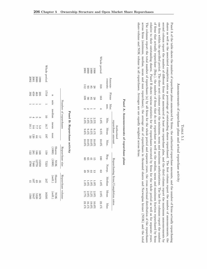
206 Chapter 5 Ownership Structure and Open Market Share Repurchases
Table
5.1
Announcem
entsof
repurchaseplans
andactual
repurchaseactivity
Panel
Aofth
eta
ble
show
sth
enum
ber
ofrep
urch
ase
pla
ns
announced
by
firm
s,th
eauth
orized
repurch
ase
am
ounts,
and
the
num
ber
offirm
sactu
ally
repurch
asin
g
shares
as
well
as
the
asso
ciated
com
pletio
nra
tesas
percen
tage
of
outsta
ndin
gsh
ares
repurch
ased
.T
he
first
colu
mn
report
the
num
ber
of
announcem
ents,
the
second
colu
mn
report
the
num
ber
ofdiff
erent
firm
sth
at
announced
at
least
one
repurch
ase
pla
n,and
the
third
colu
mn
report
the
maxim
um
announcem
ents
by
one
firm
with
inth
esp
ecified
perio
d.
The
three
nex
tco
lum
ns
report
the
min
imum
,m
ean
and
maxim
um
auth
oriza
tions.
The
last
five
colu
mns
report
the
num
ber
of
firm
sth
at
actu
ally
repurch
ase
(Rep
.),th
enum
ber
of
firm
sth
at
do
not
repurch
ase
as
well
as
the
med
ian,m
ean
and
maxim
um
fractio
nrep
urch
ased
by
firm
s
relativ
eto
their
outsta
ndin
gsh
ares.
Panel
Bsh
ows
vario
us
statistics
for
the
repurch
ases
execu
tedby
firm
sfo
rth
ew
hole
perio
das
well
as
for
separa
teyea
rs.
The
colu
mns
report
the
tota
lnum
ber
ofrep
urch
ases
(n)
by
all
firm
sfo
rth
ew
hole
perio
dand
separa
teyea
rs,th
ecro
sssectio
naldistrib
utio
nofth
erep
urch
ases
acro
ssfirm
s(m
inim
um
,m
edia
n,
mea
nand
max
repurch
ases),
the
avera
ge
sizeof
repurch
ases
inth
ousa
nd
shares
and
Norw
egia
nkro
ner
(NO
K)
and
the
tota
l
share-v
olu
me
and
NO
Kvolu
me
inall
repurch
ases.
Avera
ges
are
are
equally
weig
hted
acro
ssfirm
s.
PanelA
:A
nnouncem
ents
ofrepurchase
pla
ns
Auth
orized
repurch
ase
am
ount
Rep
urch
asin
gfirm
s/C
om
pletio
nra
tesA
nnoun-
Firm
sM
ax
cemen
tsann.
Min
.M
ean
Max.
Rep
.N
orep
.M
edia
nM
ean
Max
Whole
perio
d318
163
41.0
%9.5
%10.0
%100
63
1.8
%2.9
%22.1
%
1998
28
28
12.5
%9.1
%10.0
%15
13
1.9
%2.9
%10.0
%1999
85
85
11.0
%9.5
%10.0
%41
44
1.9
%3.2
%19.0
%2000
93
90
21.0
%9.4
%10.0
%65
25
1.8
%2.9
%16.1
%2001
112
109
23.3
%9.6
%10.0
%60
49
1.3
%2.7
%22.1
%
PanelB
:R
epurchase
activ
ity
Num
ber
ofrep
urch
ases
Rep
urch
ase
sizeR
epurch
ase
volu
me
Shares
NO
KShares
NO
Kn
min
med
ian
mea
nm
ax
(1000)
(1000)
(mill.)
(mill.)
Whole
perio
d1719
110
16.7
197
159
7223
247
16505
1999
205
13
5.0
17
168
13259
35
3679
2000
463
15
7.7
64
186
12770
65
5320
2001
659
14
9.6
120
281
7480
107
5947
2002
392
15
10.1
50
122
3780
41
1560
5.4 Data description and general statistics 207
reported by the OSE. This is due to new listings, de-listings, mergers and de-mergers oc-curring within each year.38 Overall, the average market capitalization increased throughthe period from NOK 2.3 bill. to NOK 3.4 bill, while the total market capitalization ofall listed firms increased from NOK 582 bill. in 1999 to NOK 677 bill. in 2001.39 Theaverage market-to-book value was 1.15 for all firms through the sample period. AcrossMCAP quartiles, the market-to-book value was 1.2 for the firms with a market capital-ization below the median and 1.1 for the above median firms. Further, the average cashdividend per share was the lowest in 1999, with NOK 6.1 per share, and the highest in2000 with NOK 7.6 per share. The total cash dividends paid by all firms for the periodwas NOK 40 bill., distributed across years as NOK 14 bill. in 1999, NOK 12 bill in 2000and NOK 14 bill. in 2001.40 Thus, despite the increased tax on dividends in 2001, thisdid not seem to affect the average or aggregate dividend payments by Norwegian firms.
In part (b) of table 5.2 we summarize the average ownership fraction by each of thefive largest owners. In addition, the average total fraction owned by the 5 largest ownerscombined and the Herfindahl index is reported. The first thing to note about the tableis that the average ownership fraction each of the largest owners has been relativelyconstant through the period, with the largest owner owning about 33% on average. Inaddition, the five largest owners decreased their mean ownership from 55.5% in 1999to 54.9% in 2001, while the median ownership by the five largest owners remained un-changed. These numbers are similar to what is found in Bøhren and Ødegaard (2001)for 1997 when the average stake for the largest owner was 29%, and the total ownershipby the five largest owners was 53%. However, relative to their study, the stake of thelargest owner has increased by 1.8 percentage points from 1997 to 1999, wile the aggre-gate ownership of the five largest owners increased by 2.5 percentage points. Comparedto what is common among European firms the ownership by the largest owners is verylow in Norway. Bøhren and Ødegaard (2001) report that the average ownership by thelargest owner for European countries in 1997 was 44%. When looking at the Herfindahlindex,41 this measure suggests that there was an increase in concentration from 1999 to2000, and a decrease in concentration from 2000 to 2001. However, the median concen-tration has increased through the period. For 1997 Bøhren and Ødegaard (2001) reportan average Herfindahl index of 0.15. Across market capitalizations, the most evidentpattern is that the mean fraction owned by the five largest owners is the largest in firmswith a market capitalization in the second and third quartile. This is also evident whenlooking at the Herfindahl index. With respect to the ownership of each of the largest
38The official number companies listed at the OSE at the end of each year was 215 (1999), 214 (2000),212 (2001), 203 (2002).
39In 2002 the total market capitalization of the OSE fell to NOK 503 bill.40In 2002 Norwegian firms paid out more than NOK 19 bill. in dividends.41The Herfindahl index is calculated as the sum of squared ownership fractions of all owners in a
firm. The Herfindahl index is highly correlated (more than 0.8) with the aggregate ownership of thefive largest owners.

208 Chapter 5 Ownership Structure and Open Market Share Repurchases
Table 5.2Ownership concentration and insider ownership at the OSE
Part (a) of the table shows some general statistics for the listed firms at the Oslo Stock Exchange (OSE)
across the whole sample period, separate years and market capitalization quartiles. The number of firms
also contain de-listed and firms that are listed during the sample period. Thus, this number is larger
than the number of listed firms at officially reported by the Oslo Stock Exchange at the end of the
year. The average market capitalization, Market/Book and price are monthly averages across firms.
The dividend per share is the average dividend paid by firms across the whole sample period or within
each calendar year. Part (b) of the table shows the mean and median fraction owned by the five largest
owners separately, the mean and median accumulated fraction owned by the five largest owners as well
as the Herfindahl index. Part (c) of the table shows the mean and median fraction owned by all insiders
in the firm and the primary insiders (board members and management team). Note that we only have
insider data until June 2001.
Separate years Market capitalization quartilesAll years 1999 2000 2001 Q1 Q2 Q3 Q4
(a) General statistics
Firm/year obs. 301 271 261 245 75 75 75 75MCAP (mill.NOK) 3112 2326 2818 3353 93 354 1106 11394Market/Book 1.15 1.2 1.3 1.0 1.2 1.2 1.1 1.1Price 76.0 81.6 92.3 71.2 61.2 51.0 91.4 132.0Dividend/share 6.5 6.1 7.6 7.1 8.6 7.1 8.0 5.1
(b) Ownership concentrationLargest owner
mean 0.326 0.308 0.318 0.306 0.259 0.299 0.315 0.293stddev 0.236 0.232 0.253 0.238 0.180 0.235 0.219 0.223median 0.243 0.226 0.230 0.240 0.236 0.222 0.212 0.213
2nd largestmean 0.103 0.106 0.101 0.108 0.107 0.104 0.106 0.098stddev 0.067 0.071 0.072 0.075 0.056 0.075 0.065 0.066median 0.090 0.091 0.085 0.094 0.097 0.094 0.094 0.080
3rd largestmean 0.060 0.063 0.059 0.061 0.065 0.062 0.062 0.057stddev 0.034 0.037 0.036 0.042 0.031 0.039 0.034 0.034median 0.053 0.055 0.052 0.053 0.059 0.057 0.056 0.048
4th largestmean 0.042 0.044 0.041 0.042 0.048 0.042 0.045 0.040stddev 0.022 0.024 0.024 0.024 0.023 0.023 0.026 0.019median 0.041 0.042 0.040 0.041 0.043 0.044 0.042 0.039
5th largestmean 0.032 0.034 0.032 0.032 0.036 0.033 0.033 0.032stddev 0.016 0.018 0.018 0.017 0.016 0.018 0.018 0.014median 0.032 0.033 0.032 0.032 0.035 0.035 0.032 0.032
Sum 5 largestmean 0.563 0.555 0.551 0.549 0.515 0.540 0.562 0.520stddev 0.229 0.234 0.243 0.240 0.208 0.240 0.231 0.212median 0.557 0.557 0.552 0.558 0.557 0.550 0.554 0.454
Herfindahl indexmean 0.206 0.187 0.201 0.184 0.130 0.181 0.187 0.170stddev 0.228 0.218 0.250 0.232 0.146 0.226 0.201 0.203median 0.099 0.095 0.098 0.103 0.096 0.096 0.099 0.081
(c) Insider ownershipAll insiders
mean 0.136 0.144 0.149 0.146 0.153 0.171 0.155 0.139stddev 0.253 0.264 0.273 0.269 0.279 0.287 0.262 0.266median 0.011 0.005 0.014 0.013 0.013 0.009 0.024 0.013
Primary insidersmean 0.079 0.081 0.085 0.089 0.100 0.103 0.095 0.054stddev 0.192 0.198 0.210 0.216 0.241 0.239 0.215 0.122median 0.001 0.000 0.002 0.003 0.003 0.001 0.005 0.002
Data from all listed firms at the Oslo Stock Exchange (OSE) over the period 1999-2002. Data source: Verdipa-
pirsentralen (VPS).

5.5 Descriptive analysis of ownership in repurchasing firms 209
owners across market capitalizations, the average ownership is generally the highest forfirms in the third size quartile. However, the median ownership is the largest in thelowest size quartile.
In part (c) of table 5.2 we report similar statistics for the fraction owned by insidersin firms listed on the OSE. Before we continue, it should be noted that we only haveinsider data until the first half of 2001. For the entire sample period, all insiders ownedabout 14% in Norwegian firms on average, while primary insiders (the management teamand board members) owned on average about 8%. Comparably, Bøhren and Ødegaard(2001) report that all insiders owned on average 10% in 1997 while primary insidersowned about 3%. Thus, relative to their numbers, there has been an increase in theinsider ownership at the OSE. However, some caution should be used when interpretingthese numbers since the larger insider fractions in this study may be because of the dataproblem related to the insider holdings discussed earlier. With respect to the medianinsider, all insiders owned about 1.1%, while primary insiders owned about 0.1%. Thusthe distribution of inside ownership is highly skewed. This is caused by a large part ofthe sample firms having a very low or a close to zero fraction owned by insiders of thefirm, in addition to several firms having a very high insiders ownership. Furthermore,across market capitalization quartiles, the average insider ownership is the highest inthe lowest size quartiles.
5.5 Descriptive analysis of ownership in repurchasing firms
In this section we combine the data on announcements of repurchase plans, actualrepurchases and the ownership data to examine whether there are differences in theownership composition in announcing versus non-announcing firms. In addition, weexamine whether firms that actually repurchase shares during the repurchase periodand those that do not are different from firms that do not announce a repurchase plan.To facilitate this, we split all the firms at the OSE into 4 subgroups. When looking atthe whole sample period, the first group consists of all firms that do not announce arepurchase plan during our sample period from 1999 through 2001. The second groupconsists of firms that do announce at least one repurchase plan during our sampleperiod. The third group consists of firms that announce a repurchase plan, but donot repurchase any shares during the repurchase period, and the fourth group consistsof announcing firms that actually execute repurchases during the repurchase period.42
Similarly, when looking at separate years, we split firms into groups based on whetherthey have announced a repurchase plan or not during the respective year. To determinewhether a firm has repurchased any shares after it has announced within in a specificyear, we track whether it has repurchased within the announced time limit, or within
42The repurchase period is the period for which the firm has announced that it may repurchase shares.The maximum legal limit is 18 months.
210 Chapter 5 Ownership Structure and Open Market Share Repurchases
the legal limit of 18 months. For example, a firm that announces a repurchase plan inMay of 1999 is considered a repurchasing firm (for that year) if it executes at least onerepurchase before December 2000.
5.5.1 Ownership concentration in repurchasing firms
Jensen and Meckling (1976) and Shleifer and Vishny (1986), among others, suggest thatownership concentration is an important mechanism for disciplining and monitoring non-owner managers. This because large outside owners potentially both have the incentivesto monitor through high cash flow rights as well as the power to affect corporate decisionsthrough their voting rights. If there are no large shareholders with these incentives,there may be insufficient monitoring of managers. In those cases, payout policy is onemechanism that can help reduce the agency problems as suggested by Jensen (1986).Although cash dividends and new debt also reduce the amount of free cash within afirm, more flexible repurchases may be especially attractive for firms with volatile cashflows that want to smooth dividends.
In this section we examine the ownership concentration of repurchasing firms toinvestigate whether firms with potentially higher agency problems tend to use morerepurchases. Table 5.3 shows the concentration statistics across firm-groups for thewhole period as well as for separate years. We do not distinguish between voting andnon-voting shares in any part of the analysis, but instead calculate the statistics at thecompany level.43 We calculate average statistics for the groups discussed above, where“All OSE firms” are all listed firms at the OSE. These firms are further divided into“Non-announcing firms” and “Announcing firms” depending on whether the firm hasannounced a repurchase plan during the sample period or not. The “Announcing firms”group is then further divided into two sub-groups depending on whether the firms haveexecuted any repurchases during the repurchase period (“Repurchase”) or not (“Norepurchase”). The second column in the table report the number of firms in each groupand sub-group.44 Column three to seven show the average fraction owned by the largest(ranking 1) to the fifth largest (ranking 5) owner. The eight and ninth column reportthe ownership concentration measures which is the combined fraction owned by the 5largest owners and the Herfindahl index respectively. Finally, the three last columnsreport the average market capitalization (in NOK mill.), the average dividend (in NOKper share) paid out by the firms, and the market to book value. We run tests fordifferences in means between the group of announcing firms and non-announcing firms.In addition, for the two subgroups of repurchasing and non-repurchasing firms we run atest for differences in means against the group of non-announcing firms. Thus, all tests
43Only 13 firms had non-voting (B-shares) shares at the end of 1999. During the sample period, manyfirms chose to merge these together into a single share-class.
44Note that the number of firms within each group is lower than in table 5.1. This is because thenumbers are at company level, which reduces the number of observations with about 10.

5.5 Descriptive analysis of ownership in repurchasing firms 211
are relative to the non-announcing group.45
Looking at the statistics for the whole period first, there are several things to note.The largest owner has a significantly lower stake in announcing firms (30%) than in non-announcing firms (43%). On the other hand, the second- to fifth largest owners owns asignificantly larger fraction in announcing firms than in non-announcing firms. This isalso reflected in the concentration measure in column eight (“Sum 5 largest”), where wesee that the average fraction owned by the five largest owners is significantly lower inannouncing firms than in firms that do not announce a repurchase plan. This differenceis mainly due to the lower ownership by the largest owner in these firms. With respectto the Herfindahl index the difference becomes even more pronounced. When examiningthe group of announcing firms in more detail, we see that the differences in ownershipconcentration is the largest for firms that actually repurchase shares. Looking at thefraction owned by the five largest shareholders together, we see that while the firmsthat announce, but do not repurchase has on average a combined ownership of about58% which is not significantly different from firms that do not announce a repurchaseplan (63%). However, firms that announce and repurchase has a combined ownership ofabout 53%, which is significantly lower than the group of non-announcing firms. This isalso evident when looking at the Herfindahl index. However, relative to that measure,both repurchasing and non repurchasing firms have a significantly lower concentration.For the separate years, the differences seem to be more pronounced in the last part ofthe sample, except for the ownership of the largest owner and the Herfindahl index.
These findings is in line with a story where firms with dispersed ownership havegreater incentives to initiate a self-disciplinary mechanism to ensure their shareholdersthat they are committed to mitigate agency costs of free cash. This because the largestshareholder also has potentially lower incentives to monitor management, as well as lesspower to intervene, compared to non-announcing firms where the largest shareholdersown a significantly higher fraction of the firm. In addition, the shareholders in thesefirms may also be more likely to support a proposal that the firm wants to initiate arepurchase program if it is expected to reduce agency costs.
Furthermore, the results also suggest that these differences in concentration is thestrongest in firms that actually repurchase shares. This results may however also be inline with managers using repurchases to reduce the probability of a successful hostiletakeover, and aim at increasing the ownership concentration over time in the hands ofthemselves and/or the most “manager-loyal” shareholders. In addition, as discussed
45The test depends on whether the population variances of the two groups are equal or not. If thevariances are equal, then the t-stat is calculated as t = (xa − xb)/
√s2(1/na + 1/nb) where xa and xb
are the means for the two groups respectively, na and nb are the number of firms in each group whiles2 is the pooled standard deviation calculated as s2 = [(na − 1)s2
a + (nb − 1)s2b]/[na + nb − 2], where
s2a and s2
b are the standard deviation of the ownership variable for the non-announcing and announcingfirms respectively. We use the SAS v.8.2 package to perform all tests. If the variances are significantlydifferent, the standard approximation (Satterwaite) supplied in SAS is used.

212 Chapter 5 Ownership Structure and Open Market Share Repurchases
Table
5.3
Ow
nershipconcentration
forrepurchasing
vs.non-repurchasing
firms
Inth
eta
ble
we
exam
ine
ownersh
ipva
riables
and
oth
erch
ara
cteristicsacro
ssdiff
erent
gro
ups
of
firm
s.W
esp
litfirm
sin
tofive
gro
ups.
“A
llO
SE
firm
s”are
all
firm
slisted
on
the
OSE
.T
hese
firm
sare
div
ided
into
two
gro
ups.
The
first
gro
up
is“N
on
announcin
gfirm
s”co
nta
inin
gall
firm
slisted
at
the
OSE
that
does
not
announce
arep
urch
ase
pla
ndurin
gour
sam
ple
perio
d.
The
second
gro
up
is“A
nnouncin
gfirm
s”w
hich
consists
of
firm
sth
at
announce
arep
urch
ase
pla
n.
This
gro
up
isfu
rther
div
ided
into
firm
sth
at
announce,
but
do
not
repurch
ase
any
shares
(“N
orep
urch
ase”
)and
firm
sth
at
announce
and
repurch
ase
shares
(“R
epurch
ase”
).For
the
separa
teyea
rs,“announcin
gfirm
s”are
firm
sth
at
announce
arep
urch
ase
pla
nth
at
yea
r.R
epurch
asin
gfirm
sare
firm
sth
at
announce
a
repurch
ase
pla
nth
at
result
inrep
urch
ases
with
inth
enex
trep
urch
ase
perio
d(m
ax.
18
month
s).T
he
table
show
sth
eav
erage
ownersh
ipfra
ction
for
the
5la
rgest
owners,
with
the
larg
estow
ner
hav
ing
rank
1.
Inadditio
n,w
eex
am
ine
the
com
bin
edfra
ction
owned
by
the
5la
rgest
owners
(Sum
1-5
),th
eH
erfindahlin
dex
(sum
ofsq
uared
ownersh
ipfra
ctions
ofall
owners),
the
avera
ge
mark
etva
lue
(MC
AP
)in
NO
Km
illions,
the
avera
ge
yea
rlydiv
iden
d(p
ersh
are)
paid
by
firm
sand
the
mark
etto
book
valu
e(m
ark
etca
pita
lizatio
ndiv
ided
by
the
book
valu
eofeq
uity
).W
etest
wheth
erth
ereare
diff
erences
inm
eans
for
the
vario
us
varia
bles
betw
een
firm
sth
at
announce
arep
urch
ase
pla
n(“
Announcin
gfirm
s”)
and
firm
sth
at
do
not
(“N
on
announcin
gfirm
s”).
Inadditio
n,w
ealso
testw
heth
erth
em
eans
of
the
announcin
gfirm
sth
at
repurch
ase
and
those
that
do
not
are
diff
erent
from
the
non-a
nnouncin
ggro
up.
Sig
nifi
cance
at
the
1%
,5%
and
10%
isden
oted
by∗∗∗,
∗∗and∗
respectiv
ely.
Larg
estow
ner
rankin
gSum
5H
erfindahl
MC
AP
Div
iden
dM
ark
etto
Firm
gro
up
Firm
s1
23
45
larg
estin
dex
(mill.)
(pr.sh
are)
Book
Whole
sam
ple
All
OSE
firm
s301
0.3
65
0.0
98
0.0
56
0.0
39
0.0
30
0.5
89
0.2
52
3112
6.5
1.1
5N
on
announcin
gfirm
s152
0.4
29
0.0
91
0.0
49
0.0
33
0.0
25
0.6
28
0.3
27
3567
8.5
1.1
6A
nnouncin
gfirm
s149
0.3
01∗∗∗
0.1
04∗
0.0
63∗∗∗
0.0
45∗∗∗
0.0
35∗∗∗
0.5
49∗∗∗
0.1
76∗∗∗
2693
5.4∗
1.1
4-N
orep
urch
ase
54
0.3
42∗∗
0.0
99
0.0
60∗∗
0.0
44∗∗∗
0.0
35∗∗∗
0.5
81
0.2
20∗∗
1880
5.1
1.1
5-R
epurch
ase
95
0.2
77∗∗∗
0.1
07∗∗
0.0
65∗∗∗
0.0
45∗∗∗
0.0
35∗∗∗
0.5
31∗∗∗
0.1
52∗∗∗
3155
5.6
1.1
4
Year
1999
All
OSE
firm
s271
0.3
19
0.1
04
0.0
62
0.0
44
0.0
34
0.5
62
0.2
00
2326
6.1
1.2
2N
on
announcin
gfirm
s193
0.3
33
0.1
01
0.0
61
0.0
43
0.0
33
0.5
72
0.2
20
2030
7.7
1.2
3A
nnouncin
gfirm
s78
0.2
84∗∗
0.1
11
0.0
62
0.0
44
0.0
36
0.5
38
0.1
51∗∗∗
2944∗
3.4∗∗
1.1
9-N
orep
urch
ase
39
0.3
07
0.1
08
0.0
61
0.0
44
0.0
35
0.5
54
0.1
82
1648
3.0∗∗∗
1.1
5-R
epurch
ase
39
0.2
61∗∗
0.1
14
0.0
64
0.0
45
0.0
37
0.5
21
0.1
17∗∗∗
4274
3.6∗∗∗
1.2
3
Year
2000
All
OSE
firm
s261
0.3
26
0.1
01
0.0
58
0.0
41
0.0
32
0.5
58
0.2
11
2818
7.6
1.2
6N
on
announcin
gfirm
s181
0.3
55
0.0
99
0.0
57
0.0
38
0.0
29
0.5
78
0.2
45
2347
8.1
1.2
7A
nnouncin
gfirm
s80
0.2
61∗∗∗
0.1
05
0.0
62
0.0
47∗∗∗
0.0
36∗∗∗
0.5
11
0.1
32∗∗∗
3741
6.9
1.2
5-N
orep
urch
ase
20
0.2
49∗∗
0.0
90
0.0
53
0.0
40
0.0
33
0.4
65∗∗
0.1
21∗∗
3310
9.3
1.2
5-R
epurch
ase
60
0.2
63∗∗∗
0.1
10
0.0
65∗∗
0.0
49∗∗∗
0.0
37∗∗∗
0.5
27
0.1
36∗∗∗
3884
6.5∗∗∗
1.2
5
Year
2001
All
OSE
firm
s245
0.3
13
0.1
06
0.0
60
0.0
41
0.0
32
0.5
52
0.1
93
3353
7.1
0.9
9N
on
announcin
gfirm
s145
0.3
48
0.0
99
0.0
53
0.0
37
0.0
28
0.5
65
0.2
38
4232
8.9
0.9
7A
nnouncin
gfirm
s100
0.2
62∗∗∗
0.1
14∗
0.0
704∗∗∗
0.0
48∗∗∗
0.0
37∗∗∗
0.5
33
0.1
28∗∗∗
2255
4.9∗∗∗
1.0
0-N
orep
urch
ase
47
0.2
74∗
0.1
13
0.0
68∗∗
0.0
48∗∗∗
0.0
39∗∗∗
0.5
44
0.1
38∗∗∗
1863
4.2∗∗∗
0.9
9-R
epurch
ase
53
0.2
51∗∗∗
0.1
16
0.0
72∗∗∗
0.0
47∗∗∗
0.0
36∗∗∗
0.5
24
0.1
19∗∗∗
2603
5.3∗∗
1.0
1
5.5 Descriptive analysis of ownership in repurchasing firms 213
earlier, those shareholders selling their shares in the market would also be those withthe lowest valuations effectively increasing the price to a bidder. This may indicate thatfirms where the incentives to monitor are the lowest and the probability of a successfultakeover is the highest, are more likely to actually repurchase. We will also come backto this issue when we later examine the number of owners in these firms.
The finding that the 2nd-5th largest owners have a higher ownership fraction inannouncing firms seem to be the case both for non-repurchasing and repurchasing firms.This indicates that announcing firms have a flatter power structure than non-announcingfirms. Furthermore, dispersion in ownership among the largest shareholders is evenmore pronounced in firms that actually repurchase shares. In non-announcing firms,the largest shareholder has about 2 times the stake of the combined ownership of the2nd-5th largest owners, while this ratio is 1.5 in firms that announce a repurchaseplan, and closer to 1 in firms that actually repurchase shares indicating that the largestowner has a similar stake as the 2nd-5th owners combined. The difference betweenannouncing and non-announcing firms may reflect that it is easier to obtain enoughvotes for initiating a repurchase plan in these firms than in non-announcing firms in thesense that it would be more difficult for a large shareholder to block a proposal of arepurchase program when his relative ownership is low. With respect to why firms thatactually repurchase shares has the flattest structure, this may reflect that managershave stronger incentives to actually repurchase shares in these firms. For example, themanager may benefit from concentrating the ownership in these firms to reduce theprobability of experiencing a successful takeover. Alternatively, it may also reflect thatmanagers in fact are committed to distribute excess cash in firms with the potentiallyhighest agency costs.
With respect to the size of the firms in the different groups, there is no significantdifference in market capitalization between announcing and non-announcing firms forthe whole sample or separate years. Also with respect to dividends, the difference isonly significant at the 10% level for the whole sample period. For the separate yearshowever, firms that announced repurchase plans paid significantly lower dividends bothin 1999 and 2001, but not in 2000. Looking at the subgroups of announcing firms withineach year, firms that actually repurchased shares paid significantly lower dividends thannon-announcing firms within each year. This is what one would expect to see if firmssubstitute repurchases for dividends as suggested by Grullon and Michaely (2002). Inaddition, for announcing firms that did not repurchase, the lower dividend paymentsmay be explained by these firms being less liquid, and thus less likely to pay eitherdividends or repurchase shares.46 In addition, as discussed earlier in the paper, an 11%dividend tax was introduced in 2001. This does not seem to have an impact on the
46In a previous paper on repurchases in Norway, we find that announcing firms that do not repurchaseshares has a significantly lower quick ratio and current ratio than firms that actually repurchase shares.
214 Chapter 5 Ownership Structure and Open Market Share Repurchases
average dividend payment by firms. With respect to the market to book values, theseare not significantly different for firms in any of the groups.
Overall, there seem to be systematic differences in the ownership concentration offirms that initiate a repurchase program relative to firms that do not. Repurchasingfirms generally have a much lower concentration and a flatter power structure betweenthe five largest owners. This may support several theories. One interpretation may bethat these firms may suffer from insufficient monitoring such that a repurchase planis used to mitigate agency problems related to free cash. In addition, shareholders inthese firms may be more likely to vote for a repurchase program if they believe thiswill help mitigate agency problems when there is insufficient monitoring. However, itmay be difficult to force a manager to actually repurchase shares if he prefers to keepcash within the firm. On the other hand, as suggested by Isagawa (2000), if managershave a stake in the firm, through share ownership or stock options, it may be optimalfor them to disgorge excess cash through repurchases instead of investing in negativenet present value projects that would decrease the value of the firm in the long run.Another interesting finding is that firms that actually repurchase shares have a muchflatter power structure among the five largest owners compared to any other group. Thismay suggest that managers have the strongest incentives to actually execute repurchasesin firms with low concentration.
5.5.2 Ownership by owner-types and number of owners in repurchas-
ing firms
The type of owner may also have important implications for the corporate governance ofa firm. As discussed in Bøhren and Ødegaard (2001), agency theory predicts that per-sonal owners are better monitorers than non-personal owners such as other corporationsor the state. This because, personal owners have direct private cash flow interests, whilenon-personal owners, being an agent representing the ultimate owner, do not. Thus,the incentives for monitoring management may be stronger for personal owners. On theother hand, personal owners are generally much smaller, and has less power in affectingthe decisions unless they co-ordinate their interests. In addition, it may be that sometypes of owners that have a stronger preference for one type of payout policy due toe.g. tax reasons. As suggested in Brav et al. (2003), executives do not believe that insti-tutional investors have a preference between dividends or repurchases, but that personalshareholders have a preference towards dividends despite the tax disadvantage to thispayout method in the US. On the other hand, their study suggest that institutions oftenhave an important influence with respect to initiating a repurchase program.
In this section we examine the ownership by different owner types both with respectto their proportional ownership as well as to the number of owners by different types.Our dataset has information on 5 main types of owners; State owners that represent

5.5 Descriptive analysis of ownership in repurchasing firms 215
investments by the central or local government, foreign owners47 which reflect owner-ship by non-resident organizations or individuals, financial owners reflects institutionalownership such as private banks, insurance firms, pension funds and investment trusts,Nonfinancial owners are domestic firms, and individuals which are Norwegian personalinvestors.
In table 5.4 we calculate the average ownership fractions owned by these owner-types for the same groups that we used in the previous section. For all firms at theOSE, the largest average owner is non-financial, which is also the result in Bøhrenand Ødegaard (2001). With respect to the difference in ownership fraction betweenannouncing and non-announcing firms, there are only two types that have a significantlydifferent ownership in announcing firms for the whole period. These are foreignerswhich has a significantly lower stake in announcing firms, while non-financial ownershas a significantly higher stake in announcing firms. In both cases this is mainly due totheir ownership in firms that actually execute repurchases. In addition, the differenceis strongest for firms announcing and repurchasing in the beginning of the sample.
Whether these differences are because certain ownertypes has a preference for oragainst repurchases, or that firms with these types of owners initiate repurchases isdifficult to say. However, one may speculate that one reason for this might be thatforeign owners are mutual funds or other foreign investors that are invested in Norwayfor diversification reasons. As we saw in table 5.3 for the whole sample period, announc-ing firms seemed to have a slightly smaller (although insignificantly different) marketcapitalization than non-announcing firms. If foreign investors are tracking the valueweighted return on the OSE, they are also likely to be invested in the largest firms onthe exchange. A potential reason for why nonfinancial owners has a greater stake in re-purchasing firms may be that some firms use their repurchased shares (treasury shares)as payment in transactions with other firms. In addition, the reason may simply bethat the treasury stock is captured in this measure such that the numbers also reflectthat firms own their own stock.48
Another statistic that represent an alternative measure of concentration is the num-ber of owners. One problem with the average ownership fraction by different ownertypes, examined in table 5.4, is that it may to a large degree capture the ownership bythe largest owners of a type. The number of owners by different owner types may giveadditional information with respect to the preferences of different shareholder groups.In table 5.5 we examine the average number of owners by owner type across the differentfirm groups as well as the mean total number of owners. Compared to the previous table
47The number of foreign owners is understated because it contain both registered individuals as wellas nominee accounts which may reflect several different owners.
48We do not examine in what degree the firms own stock contribute to the difference. Since theowners in the VPS data are anonymized and represented by a unique number, it is difficult to removethe repurchasing firms own shareholdings.
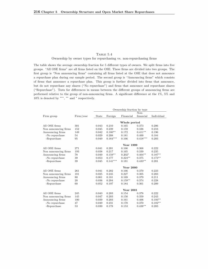
216 Chapter 5 Ownership Structure and Open Market Share Repurchases
Table 5.4Ownership by owner types for repurchasing vs. non-repurchasing firms
The table shows the average ownership fraction for 5 different types of owners. We split firms into five
groups. “All OSE firms” are all firms listed on the OSE. These firms are divided into two groups. The
first group is “Non announcing firms” containing all firms listed at the OSE that does not announce
a repurchase plan during our sample period. The second group is “Announcing firms” which consists
of firms that announce a repurchase plan. This group is further divided into firms that announce,
but do not repurchase any shares (“No repurchase”) and firms that announce and repurchase shares
(“Repurchase”). Tests for differences in means between the different groups of announcing firms are
performed relative to the group of non-announcing firms. A significant difference at the 1%, 5% and
10% is denoted by ∗∗∗, ∗∗ and ∗ respectively.
Ownership fraction by typeNon-
Firm group Firm/year State Foreign Financial financial Individual
Whole periodAll OSE firms 301 0.043 0.210 0.165 0.373 0.206Non announcing firms 152 0.045 0.239 0.159 0.336 0.216Announcing firms 149 0.042 0.180∗∗ 0.172 0.411∗∗ 0.196
-No repurchase 54 0.029 0.208 0.181 0.400 0.184-Repurchase 95 0.049 0.164∗∗∗ 0.166 0.418∗∗∗ 0.203
Year 1999All OSE firms 271 0.041 0.201 0.166 0.368 0.222Non announcing firms 193 0.038 0.217 0.165 0.339 0.235Announcing firms 78 0.049 0.159∗∗ 0.202∗ 0.404∗∗ 0.187∗∗
-No repurchase 39 0.053 0.177 0.224∗∗ 0.375 0.173∗∗
-Repurchase 39 0.045 0.141∗∗∗ 0.181 0.433∗∗ 0.201
Year 2000All OSE firms 261 0.041 0.202 0.166 0.370 0.223Non announcing firms 181 0.025 0.245 0.227 0.305 0.203Announcing firms 80 0.061 0.181 0.169 0.379 0.211
-No repurchase 20 0.036 0.204 0.159∗∗ 0.374 0.228-Repurchase 60 0.052 0.197 0.184 0.361 0.209
Year 2001All OSE firms 245 0.043 0.203 0.154 0.378 0.222Non announcing firms 145 0.047 0.203 0.150 0.359 0.243Announcing firms 100 0.039 0.203 0.161 0.406 0.193∗∗
-No repurchase 47 0.049 0.231 0.170 0.370 0.182∗∗
-Repurchase 53 0.030 0.178 0.153 0.438∗∗ 0.203
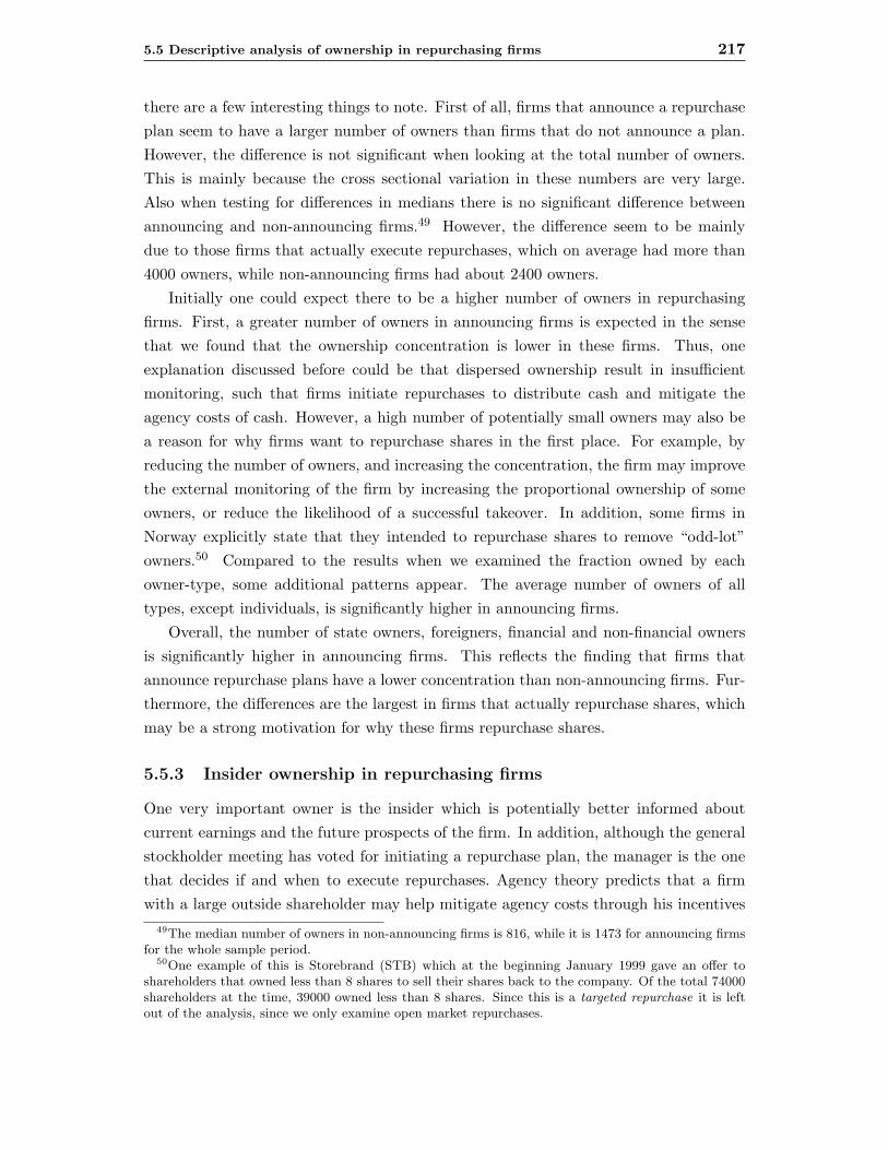
5.5 Descriptive analysis of ownership in repurchasing firms 217
there are a few interesting things to note. First of all, firms that announce a repurchaseplan seem to have a larger number of owners than firms that do not announce a plan.However, the difference is not significant when looking at the total number of owners.This is mainly because the cross sectional variation in these numbers are very large.Also when testing for differences in medians there is no significant difference betweenannouncing and non-announcing firms.49 However, the difference seem to be mainlydue to those firms that actually execute repurchases, which on average had more than4000 owners, while non-announcing firms had about 2400 owners.
Initially one could expect there to be a higher number of owners in repurchasingfirms. First, a greater number of owners in announcing firms is expected in the sensethat we found that the ownership concentration is lower in these firms. Thus, oneexplanation discussed before could be that dispersed ownership result in insufficientmonitoring, such that firms initiate repurchases to distribute cash and mitigate theagency costs of cash. However, a high number of potentially small owners may also bea reason for why firms want to repurchase shares in the first place. For example, byreducing the number of owners, and increasing the concentration, the firm may improvethe external monitoring of the firm by increasing the proportional ownership of someowners, or reduce the likelihood of a successful takeover. In addition, some firms inNorway explicitly state that they intended to repurchase shares to remove “odd-lot”owners.50 Compared to the results when we examined the fraction owned by eachowner-type, some additional patterns appear. The average number of owners of alltypes, except individuals, is significantly higher in announcing firms.
Overall, the number of state owners, foreigners, financial and non-financial ownersis significantly higher in announcing firms. This reflects the finding that firms thatannounce repurchase plans have a lower concentration than non-announcing firms. Fur-thermore, the differences are the largest in firms that actually repurchase shares, whichmay be a strong motivation for why these firms repurchase shares.
5.5.3 Insider ownership in repurchasing firms
One very important owner is the insider which is potentially better informed aboutcurrent earnings and the future prospects of the firm. In addition, although the generalstockholder meeting has voted for initiating a repurchase plan, the manager is the onethat decides if and when to execute repurchases. Agency theory predicts that a firmwith a large outside shareholder may help mitigate agency costs through his incentives
49The median number of owners in non-announcing firms is 816, while it is 1473 for announcing firmsfor the whole sample period.
50One example of this is Storebrand (STB) which at the beginning January 1999 gave an offer toshareholders that owned less than 8 shares to sell their shares back to the company. Of the total 74000shareholders at the time, 39000 owned less than 8 shares. Since this is a targeted repurchase it is leftout of the analysis, since we only examine open market repurchases.
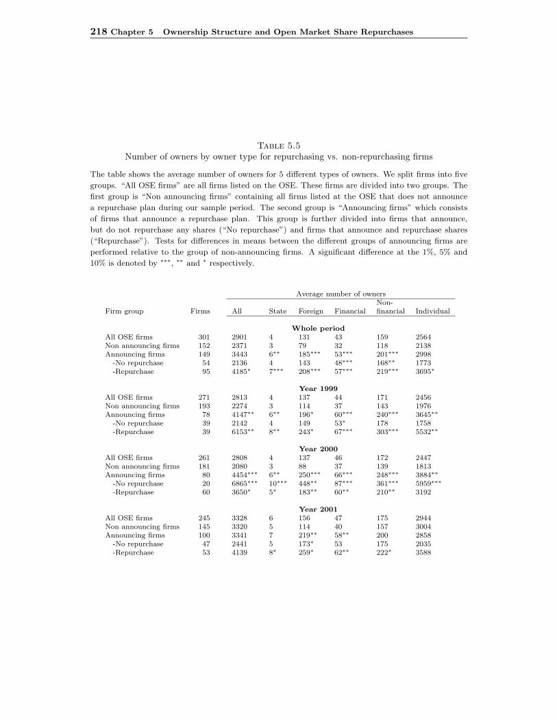
218 Chapter 5 Ownership Structure and Open Market Share Repurchases
Table 5.5Number of owners by owner type for repurchasing vs. non-repurchasing firms
The table shows the average number of owners for 5 different types of owners. We split firms into five
groups. “All OSE firms” are all firms listed on the OSE. These firms are divided into two groups. The
first group is “Non announcing firms” containing all firms listed at the OSE that does not announce
a repurchase plan during our sample period. The second group is “Announcing firms” which consists
of firms that announce a repurchase plan. This group is further divided into firms that announce,
but do not repurchase any shares (“No repurchase”) and firms that announce and repurchase shares
(“Repurchase”). Tests for differences in means between the different groups of announcing firms are
performed relative to the group of non-announcing firms. A significant difference at the 1%, 5% and
10% is denoted by ∗∗∗, ∗∗ and ∗ respectively.
Average number of ownersNon-
Firm group Firms All State Foreign Financial financial Individual
Whole periodAll OSE firms 301 2901 4 131 43 159 2564Non announcing firms 152 2371 3 79 32 118 2138Announcing firms 149 3443 6∗∗ 185∗∗∗ 53∗∗∗ 201∗∗∗ 2998
-No repurchase 54 2136 4 143 48∗∗∗ 168∗∗ 1773-Repurchase 95 4185∗ 7∗∗∗ 208∗∗∗ 57∗∗∗ 219∗∗∗ 3695∗
Year 1999All OSE firms 271 2813 4 137 44 171 2456Non announcing firms 193 2274 3 114 37 143 1976Announcing firms 78 4147∗∗ 6∗∗ 196∗ 60∗∗∗ 240∗∗∗ 3645∗∗
-No repurchase 39 2142 4 149 53∗ 178 1758-Repurchase 39 6153∗∗ 8∗∗ 243∗ 67∗∗∗ 303∗∗∗ 5532∗∗
Year 2000All OSE firms 261 2808 4 137 46 172 2447Non announcing firms 181 2080 3 88 37 139 1813Announcing firms 80 4454∗∗∗ 6∗∗ 250∗∗∗ 66∗∗∗ 248∗∗∗ 3884∗∗
-No repurchase 20 6865∗∗∗ 10∗∗∗ 448∗∗ 87∗∗∗ 361∗∗∗ 5959∗∗∗
-Repurchase 60 3650∗ 5∗ 183∗∗ 60∗∗ 210∗∗ 3192
Year 2001All OSE firms 245 3328 6 156 47 175 2944Non announcing firms 145 3320 5 114 40 157 3004Announcing firms 100 3341 7 219∗∗ 58∗∗ 200 2858
-No repurchase 47 2441 5 173∗ 53 175 2035-Repurchase 53 4139 8∗ 259∗ 62∗∗ 222∗ 3588
5.5 Descriptive analysis of ownership in repurchasing firms 219
to monitor and power to intervene in the decision process. Similarly, when the managerhas a stake in the firm, the agency problem may also be lower as there is a convergenceof interest (Jensen and Meckling, 1976) between the inside- and outside owners. How-ever, as discussed in section 5.2, there may also be a conflict between inside- and outsideowners. First of all, the manager may not have any incentives to actually execute re-purchases even though the shareholders have voted for a repurchase plan. Alternatively,the manager may have incentives to secure their position in the firm by increasing theirownership fraction (entrenchment) through repurchasing. One example would be toresist hostile takeovers that, if successful, would threaten their position in the firm andmake them loose control over the firms resources. As argued by Bagwell (1991) andothers, a repurchase may be used as an effective measure to to reduce the probability oftakeovers. For the outside owners, this would reduce their wealth if the takeover is ex-pected to be a valuable restructuring within the firm that could lead to a more efficientuse of firm resources. As shown by Denis (1990) the price effect for a firm announcinga defensive repurchase is highly negative which suggests that defensive repurchases areassociated with losses for the shareholders of the target firm.
A large part of the literature also focus argue that insiders use repurchases to conveyprivate information to the market, and that this is a potential reason for why a positiveannouncement effect is observed. Ignoring the credibility issues related to announce-ments motivated by undervaluation, discussed in Fried (2002) among others, one wouldexpect insiders to have a higher ownership in firms announcing a repurchase plan dueto mispricing, than firms that do not. Furthermore, in models by Brennan and Thakor(1990) and Barclay and Smith (1988) the manager also use repurchases to increase hisownership in an undervalued firm and thereby transfer wealth from uninformed share-holders to himself and the remaining shareholders. The model in Isagawa (2000) moreexplicitly focus on the credibility issues related of open market repurchase, and arguethat when the manager has stock options or own shares in the firm, it may be optimalfor him to initiate a repurchase program and substitute repurchases for dividends. Theprediction of these models is that firms with high insider ownership are more likely toinitiate repurchases, or that the insider ownership is expected to increase in undervaluedfirms. In line with the predictions in Isagawa (2000), Li and McNally (2002) find thatrepurchasing firms in Canada have a higher insider ownership on average. In addition,Fenn and Liang (2001) find that repurchase activity is positively related to the amountof management options in Canadian firms. They argue that their results suggest thatmanagers use repurchases to increase the value of these options by substituting repur-chases for dividends.
Further, as argued by Fried (2002), managers motivation for repurchasing sharesmay also be related to managerial opportunism. This in the sense that managers maywant to initiate an open market repurchase both when the firm is undervalued and

220 Chapter 5 Ownership Structure and Open Market Share Repurchases
overvalued, which is in contrast to the undervaluation hypothesis where the managerswant to initiate a repurchase plan only in the cases when the firm is undervalued.Relative to the undervaluation hypothesis, the manager opportunism hypothesis doesnot have any clear-cut predictions with respect to the insider ownership in repurchasingfirms unless these firms are systematically undervalued.
To investigate these issues further, table 5.6 provide statistics on the average insiderownership for all insiders as well as for primary insiders for the same groups of firms asbefore. We find a large difference in average insider ownership in firms that announcea repurchase plan relative to non-announcing firms. On average for the whole sampleperiod, insiders in announcing firms own more than twice (20%) the fraction of insidersin non-announcing firms (8%). This difference is also systematic and significant forthe separate years. However, when we examine more closely the groups of announcingfirms that actually repurchase or not, some differences appear. The results suggests thefirms that actually repurchase seem to have the highest total insider ownership of thetwo groups. This may indicate that insiders retain their shares in repurchasing firms,increasing their ownership proportion.
When looking at only the ownership by the primary insiders (managers and membersof the board), the results are similar for the whole sample period. Moreover, primaryown on average 11.5% in firms that initiate a repurchase program, but only 4.5% innon-announcing firms. For the subgroups of announcing firms, primary insiders havea higher ownership in firms that do not repurchase any shares, which is the oppositeas the result for all insiders. The difference becomes even more apparent when lookingat the separate years. We do not have a good explanation for this difference betweenprimary insiders and all insiders. When looking at separate years, the difference inprimary ownership is not significantly different for announcing firms in 2001.
Relative to the different models and hypotheses discussed earlier, this finding is con-sistent both with mispricing, entrenchment, expropriation and the model of Isagawa(2000). Relative to an agency story, where repurchases is used to mitigate agency costs,we would expect to see a lower insider ownership in announcing firms. Thus, combinedwith the findings earlier, where firms with low concentration and more dispersed own-ership initiate repurchase programs, the high insider stake may suggest that mitigationof agency costs is a less important motivation for why firms repurchase. On the otherhand, it might be that both are important reasons for why firms initiate repurchaseprograms, but that this differ among firms.
To further investigate the difference in insider ownership between announcing andnon-announcing firms we examine the distribution of insider ownership in more detail.The main reason for examining this more closely is that the insider data may overes-timate the true insider holdings. The construction of the insider data is based on the
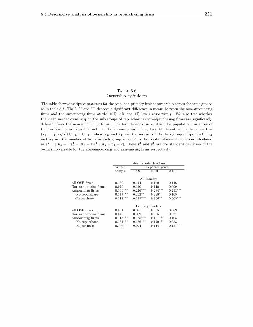
5.5 Descriptive analysis of ownership in repurchasing firms 221
Table 5.6Ownership by insiders
The table shows descriptive statistics for the total and primary insider ownership across the same groups
as in table 5.3. The ∗, ∗∗ and ∗∗∗ denotes a significant difference in means between the non-announcing
firms and the announcing firms at the 10%, 5% and 1% levels respectively. We also test whether
the mean insider ownership in the sub-groups of repurchasing/non-repurchasing firms are significantly
different from the non-announcing firms. The test depends on whether the population variances of
the two groups are equal or not. If the variances are equal, then the t-stat is calculated as t =
(xa − xb)/√
s2(1/na + 1/nb) where xa and xb are the means for the two groups respectively, na
and nb are the number of firms in each group while s2 is the pooled standard deviation calculated
as s2 = [(na − 1)s2a + (nb − 1)s2
b]/[na + nb − 2], where s2a and s2
b are the standard deviation of the
ownership variable for the non-announcing and announcing firms respectively.
Mean insider fractionWhole Separate yearssample 1999 2000 2001
All insidersAll OSE firms 0.139 0.144 0.149 0.146Non announcing firms 0.079 0.110 0.110 0.099Announcing firms 0.199∗∗∗ 0.226∗∗∗ 0.234∗∗∗ 0.212∗∗∗
-No repurchase 0.177∗∗∗ 0.202∗∗ 0.228∗ 0.109-Repurchase 0.211∗∗∗ 0.249∗∗∗ 0.236∗∗ 0.305∗∗∗
Primary insidersAll OSE firms 0.081 0.081 0.085 0.089Non announcing firms 0.045 0.059 0.065 0.077Announcing firms 0.115∗∗∗ 0.135∗∗∗ 0.131∗∗∗ 0.105
-No repurchase 0.131∗∗∗ 0.176∗∗∗ 0.179∗∗∗ 0.053-Repurchase 0.106∗∗∗ 0.094 0.114∗ 0.151∗∗
222 Chapter 5 Ownership Structure and Open Market Share Repurchases
actual reports from the transactions reported by insiders to the OSE.51 However, sinceinsiders are not required to report to the OSE when leaving the firm, or his subsequenttransactions, the holdings of these insiders persist in the data. One effect of this is thatthe insider fraction in some instances may become very high, and in some instances100%. This is of course not possible since the firm in that case would not be listed onthe OSE. Despite this bias, we do not expect there to be more extreme insider firmsamong the announcing firms than among the non-announcing firms except if insidersare more active in on of the groups. However, we want to examine the effect of this biasmore closely. To do this, we remove all firms with more than 90% insider ownership,and recalculate the insider statistics.
The results from the truncations are reported in table 5.7. In panel A of the table,we examine the cross-sectional distribution of the total insider ownership for the wholeperiod. If there is a systematic bias towards one of the groups removing the extremeobservations should make the two distributions more similar. Doing this decreases themean total insider fraction for the non-announcing firms from 8% to 7%, and for theannouncing firms from 20% to 14%. However, the difference in means is still significantat the 1% level. Also for the separate years, there is a decrease in the mean for bothgroups. For 1999 the difference in insider ownership becomes insignificant, but for 2000and 2001 it is still significant at the 1% level. When we perform the the same exercisefor the primary insiders the results go in the same direction, but the change is lesspronounced since there is fewer firms with extreme primary insider ownership.
Removing the insider fractions above 90% seems to reduce both averages similarlyfor the two groups, such that there is no systematic bias towards the announcing firms.However, an insider fraction>90% is still not uninteresting, because it captures a featurein the data in that insiders are more active in these firms. Thus, we do not remove themfrom the rest of the analysis, but acknowledge that there is a potential bias relative tothe insider data.
5.5.4 Changes in ownership in repurchasing firms
So far, we have examined the average ownership in firms that announces a repurchaseplan. We now turn to examining how the various ownership variables change during thecourse of the repurchase program. This is done by examining the ownership character-istics one month before firms executes their first repurchases, relative to the ownershipcharacteristics for the same firms 12 months and 24 months afterwards. Thus, for eachownership variable we have a cross section of values before the firms execute their firstrepurchase and a cross section of values 12 (and 24) months after the firms initial re-purchase. Note that the months vary across firms, such that the analysis is essentiallysimilar to an event study where firms that experience an event at different points in
51An insider is required to report any transaction to the OSE before 10 am the following day.

5.5 Descriptive analysis of ownership in repurchasing firms 223
Table 5.7Distribution of total insider ownership
The table shows the distribution of total insider ownership across the two groups of announcing and
non-announcing firms. In first part of panel A (“Full sample”), we use all firms in the sample. In the
second part (“Truncated”) we remove all firms that have an average insider ownership greater than 90%
for both groups. We test whether the means of the cross sectional distributions are equal with ∗, ∗∗ and∗∗∗ denoting a significant difference at the 10%, 5% and 1% levels respectively. The tests are adjusted
for differences in variances between the two distributions if the variance is significantly different. In
panel B we examine the distribution of insider ownership across firms that announce/do not announce
within each year.
Panel A: Cross sectional distribution of insider ownership - whole period
Insider ownership distribution std.devFirms p25 Median Mean P75 p90 max mean
Full sample-Non-announcing 152 0.000 0.00 0.08 0.05 0.26 1.00 0.19-Announcing 149 0.002 0.04 0.20∗∗∗ 0.27 0.70 1.00 0.30
Truncated sample-Non-announcing 144 0.000 0.00 0.07 0.04 0.24 0.88 0.16-Announcing 139 0.001 0.03 0.14∗∗∗ 0.21 0.59 0.87 0.22
Panel B: Cross sectional distribution of insider ownership - separate years
Insider ownership distribution std.devFirms p25 Median Mean P75 p90 max mean
Year 1999Full sample
-Non-announcing 193 0.000 0.00 0.11 0.08 0.39 1.00 0.22-Announcing 78 0.001 0.05 0.23∗∗∗ 0.33 0.93 1.00 0.33
Truncated sample-Non-announcing 182 0.000 0.00 0.09 0.06 0.34 0.88 0.17-Announcing 69 0.001 0.03 0.13 0.17 0.43 0.87 0.20
Year 2000Full sample
-Non-announcing 181 0.000 0.00 0.11 0.06 0.41 1.00 0.24-Announcing 80 0.003 0.06 0.23∗∗∗ 0.40 0.81 1.00 0.32
Truncated sample-Non-announcing 169 0.000 0.00 0.07 0.05 0.30 0.88 0.16-Announcing 73 0.003 0.04 0.16∗∗∗ 0.24 0.51 0.85 0.23
Year 2001Full sample
-Non-announcing 145 0.000 0.00 0.10 0.05 0.26 1.00 0.24-Announcing 100 0.003 0.06 0.21∗∗∗ 0.34 0.69 1.00 0.29
Truncated sample-Non-announcing 135 0.000 0.00 0.07 0.03 0.21 0.88 0.16-Announcing 94 0.002 0.04 0.16∗∗∗ 0.29 0.51 0.88 0.22
224 Chapter 5 Ownership Structure and Open Market Share Repurchases
time are aligned in event time. One concern with this is that there may have been atrend in the ownership variables through the sample period, and that the change reflectthese trends. However, in table 5.2 there is not any indication that there has been alarge change in the average for any of the variables across all firms at the OSE dur-ing the sample period. In addition, since different firms execute their first repurchasethroughout the entire sample period, this will mitigate the effect from a trend in theownership variables.
To examine whether there is a change in the various ownership variables before andafter the initial repurchases, we run a paired test for differences in means, where thenull hypothesis is that the cross sectional mean for each variable is equal before andafter the initial repurchase. The results from this analysis is shown in table 5.8. Theleft section of the table shows the results when we examine the change over a 12 monthperiod after the firms execute their first repurchase, while the right part of the tableshows the results for changes over a 24 month period. For each variable the table showsthe cross sectional mean one month before firms repurchase for the first time (“before”),and the mean 12 or 24 months after the initial repurchase (“after”), the p-value fromthe paired test, and an indicator for the change in the mean (“direction”). Note thatthe means before are different when we use a 12 month period from when we use a24 month period. This is because we loose observations when we examine the longestperiod since we only have ownership data through 2002 such that firms repurchasingfor the first time in 2001 drop out of the sample.
As would be expected, the repurchases increase the concentration both relative tothe total fraction owned by the 5 largest owners as well as relative to the Herfindahlindex. However, the change in the Herfindahl index is only significant at the 5% levelwhen we consider the 24 month change in the index. Relative to the separate ownershipfractions of the five largest owners, only the largest owner has a significant increasein the fraction, which suggests that the change in concentration is to a large degreeis due to the increased ownership of the largest owner. The ownership fraction of all-and primary insiders increases, but not significantly. The fraction owned by the stateincreases significantly both for the 12 and 24 month periods. One reason for this maybe that the state often is a long-term investor, and are more likely to retain its sharesthrough the repurchase period, increasing its proportional ownership when the firm re-purchase. On the other hand the ownership of institutional (financial) and individualinvestors decreases when firm repurchase shares. There may be several reasons for this.If personal investors are afraid of being expropriated (Brennan and Thakor, 1990) orhas a preference for dividends they may reduce their ownership in repurchasing firms.Alternatively, since both institutional and personal investors probably are those ownersthat trade most frequently (as opposed to the state, foreigners and other companies)among the different owner types, they are more likely to sell their shares back to the
5.6 The probability of announcement 225
company when it purchase shares in the open market. Interestingly, the decrease ininstitutional ownership is opposite of what Grinstein and Michaely (2001) find for asample of public firms in the US. Why this difference appear is difficult to say. How-ever, it may be argued that this is something one would expect to see. Shleifer andVishny (1986) argue that firms pay dividends to attract institutions. In addition, manyinstitutional investors also have restrictions with respect to investing in non-dividendpaying firms. From this point of view, one would expect institutions to reduce theirownership if firms that substitute repurchases for dividends.
Finally, when we examine the change in the number of owners of the different ownertypes, we find that the average total number of owners declines during both periods,and that there is a decrease in the number of financial, non-financial and individualowners, while the number of foreign owners is relatively stable. In addition, the numberof state owners increase during the 24 month period which reflect that these owners notonly retain their shares, but that repurchasing firms may attract investors of this type.
5.6 The probability of announcement
Having examined the ownership structure characteristics of firms that use repurchases,we now examine whether the ownership structure affect the propensity for a firm to an-nounce a repurchase plan. Thus, in this section we examine in more detail whether thereare systematic relation between the ownership structure of firms and the probability ofseeing a firm announcing a repurchase plan during the following period, conditional onownership variables at a fixed point in time. To do this we estimate a binary regressionmodel for estimating the effect of various ownership variables on the propensity for firmsto announce (Ann) a repurchase program. The general model to be estimated is,
Prob(Ann) = F(β ′x) (5.1)
where β ′x is the index function, with x containing the explanatory variables for eachfirm, β is a vector of coefficients and F(·) is the cumulative distribution function. Themodel is estimated as a binary regression model by assuming that a variable Ann∈ {1, 0},which is the event of a firm announcing a repurchase plan or not, is related to a setof explanatory variables x.52 We estimate models based on both a probit and logitspecification by maximum likelihood.53 However, since the results the two specificationsare very similar, we report only results from the logit estimation.54
52A more detailed explanation is provided in appendix 5.A.53The proc logistic, proc probit in addition to the proc mixed procedures, provided in SAS v.8.2 are
used for the numerical optimizations.54Also as noted in Greene (2000), the difference between a logit and probit specification is generally
very small unless for very large samples.
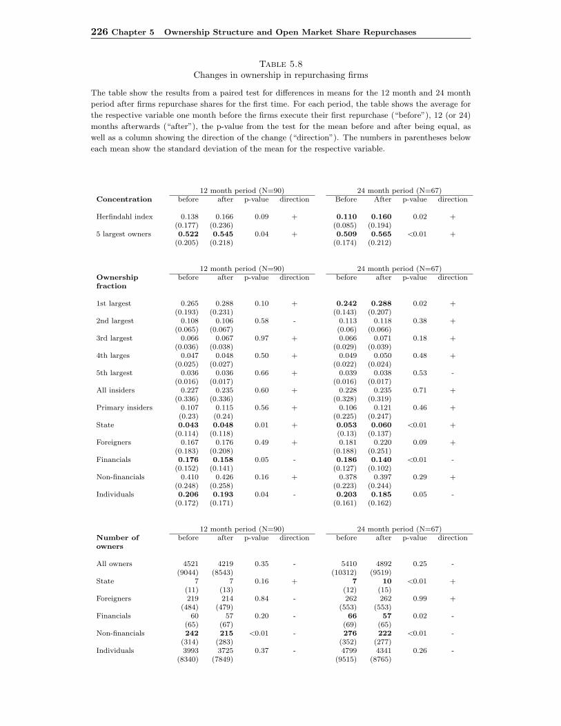
226 Chapter 5 Ownership Structure and Open Market Share Repurchases
Table 5.8Changes in ownership in repurchasing firms
The table show the results from a paired test for differences in means for the 12 month and 24 month
period after firms repurchase shares for the first time. For each period, the table shows the average for
the respective variable one month before the firms execute their first repurchase (“before”), 12 (or 24)
months afterwards (“after”), the p-value from the test for the mean before and after being equal, as
well as a column showing the direction of the change (“direction”). The numbers in parentheses below
each mean show the standard deviation of the mean for the respective variable.
12 month period (N=90) 24 month period (N=67)Concentration before after p-value direction Before After p-value direction
Herfindahl index 0.138 0.166 0.09 + 0.110 0.160 0.02 +(0.177) (0.236) (0.085) (0.194)
5 largest owners 0.522 0.545 0.04 + 0.509 0.565 <0.01 +(0.205) (0.218) (0.174) (0.212)
12 month period (N=90) 24 month period (N=67)Ownership before after p-value direction before after p-value directionfraction
1st largest 0.265 0.288 0.10 + 0.242 0.288 0.02 +(0.193) (0.231) (0.143) (0.207)
2nd largest 0.108 0.106 0.58 - 0.113 0.118 0.38 +(0.065) (0.067) (0.06) (0.066)
3rd largest 0.066 0.067 0.97 + 0.066 0.071 0.18 +(0.036) (0.038) (0.029) (0.039)
4th larges 0.047 0.048 0.50 + 0.049 0.050 0.48 +(0.025) (0.027) (0.022) (0.024)
5th largest 0.036 0.036 0.66 + 0.039 0.038 0.53 -(0.016) (0.017) (0.016) (0.017)
All insiders 0.227 0.235 0.60 + 0.228 0.235 0.71 +(0.336) (0.336) (0.328) (0.319)
Primary insiders 0.107 0.115 0.56 + 0.106 0.121 0.46 +(0.23) (0.24) (0.225) (0.247)
State 0.043 0.048 0.01 + 0.053 0.060 <0.01 +(0.114) (0.118) (0.13) (0.137)
Foreigners 0.167 0.176 0.49 + 0.181 0.220 0.09 +(0.183) (0.208) (0.188) (0.251)
Financials 0.176 0.158 0.05 - 0.186 0.140 <0.01 -(0.152) (0.141) (0.127) (0.102)
Non-financials 0.410 0.426 0.16 + 0.378 0.397 0.29 +(0.248) (0.258) (0.223) (0.244)
Individuals 0.206 0.193 0.04 - 0.203 0.185 0.05 -(0.172) (0.171) (0.161) (0.162)
12 month period (N=90) 24 month period (N=67)Number of before after p-value direction before after p-value directionowners
All owners 4521 4219 0.35 - 5410 4892 0.25 -(9044) (8543) (10312) (9519)
State 7 7 0.16 + 7 10 <0.01 +(11) (13) (12) (15)
Foreigners 219 214 0.84 - 262 262 0.99 +(484) (479) (553) (553)
Financials 60 57 0.20 - 66 57 0.02 -(65) (67) (69) (65)
Non-financials 242 215 <0.01 - 276 222 <0.01 -(314) (283) (352) (277)
Individuals 3993 3725 0.37 - 4799 4341 0.26 -(8340) (7849) (9515) (8765)
5.6 The probability of announcement 227
5.6.1 Variable selection
Before we continue, we need to select variables (x) that may be argued to be importantfor why firms initiate a repurchase plan. Since the set of ownership variables availableto us has been examined earlier in the paper, the estimation results are likely to reflectmany of the patterns found in the descriptive part. However, by estimating a model weare better able to address the relative importance of the various variables.
The first variable we include in the analysis is the insider fraction. As discussedearlier, agency theory predict that higher insider ownership align the interests of inside-and outside owners such that the need for external monitoring is reduced. In that case,the need for cash distribution to mitigate agency costs would be lower such that firmswith high insider ownership should not be expected to initiate repurchase programsas often as firms with low insider ownership. Alternatively, insiders may also want toinitiate a repurchase plan to maximize their future wealth, to increase the value of theiroptions, entrench themselves, counter takeovers or to expropriate outside shareholders.To examine whether a very high insider ownership has any effect on the propensityfor firms to initiate a repurchase program, we also create a dummy variable (“Highinsider ownership”) which is equal to 1 if the insider stake is larger than 33% and zero ifnot.55 If the insiders have a large stake in the firm, they may vote against the initiationof a repurchase program, effectively stopping it. Alternatively, they may also force arepurchase program through, if they have a strong preference for repurchases.
Another variable that is predicted by agency theory to be important for the quality ofcorporate governance is ownership concentration. A higher concentration is expected toimprove monitoring such that the need for additional mechanisms to restrict managersto waste cash, such as repurchases, are reduced. In addition, we create a dummy variableto examine whether firms with a large controlling shareholder are more or less likely toannounce a repurchase plan. The dummy variable (“Largest owner >67%”) is equal toone if the largest shareholder has a super-majority (ownership fraction > 2/3). A verylarge owner may have very strong incentives to monitor the management of the firm,reducing the need for additional mechanisms to discipline management. Alternatively,a large controlling shareholder can also effectively block the proposal of a repurchaseplan by voting against it.
We also have information about the type of the largest owner. Moreover, we knowwhether the largest owner is a state-, foreign-, financial-, nonfinancial- or individualowner. Since the identity of the largest owner may be important with respect to theincentive to monitor, we create dummies, which are interacted with the fraction ownedby the largest owner to examine this. For example, it might be that personal owners arebetter monitorers than other owners, such as large corporations or the state, because
55The threshold is not related to any theoretical predictions, but merely reflect whether insiders hasa super minority (1/3).
228 Chapter 5 Ownership Structure and Open Market Share Repurchases
the quality of the firm affect their wealth more directly. On the other hand, it may bethat institutional investors are more competent with respect to how the firm should berun and have a preference for dividend payments which would make them more inclinedto vote against the proposal of a repurchase program.
Another variable which may affect the motivation for why a firm announces a re-purchase plan is the dividend history of a firm. If firms are reluctant to reduce theirdividends and engage in dividend smoothing, as suggested by Lintner (1956) and Bravet al. (2003), a firm that has paid dividends previously may be less likely to initiatea repurchase plan if it plans on maintaining its dividend rate. In addition, the sizeof the firm may be important since larger firms generally have more shareholders andpotentially a more dispersed ownership.
In addition, we examine various model specifications to investigate whether the totalnumber of owners, the number of owners by the different owner-types as well as theirownership proportions affect the propensity for firms to announce a repurchase plan.With respect to the discussion earlier, a high number of owners may be a motivationfor firms to repurchase shares in the first place.
5.6.2 Estimation results
We estimate the models in the beginning of 1999, 2000 and 2001 with a predictionperiod of 12 months. Thus, for each year we use the most recent information before weestimate the models.56 Furthermore, all firms that were not yet listed at the beginningof the estimation year is excluded from the estimation for the respective year.
Table 5.9 report the correlations between various variables in, 1999 and 2000, thatwe examine in the various models. The lower triangular part of the table show thecorrelations for January 1999 and the upper triangular part of the table shows thecorrelations for January 2000. For each pair of variables, the table shows the correlationwith the associated p-value from a test of the correlation being equal to zero. First of all,most of the correlations are of the same magnitude and sign for the two years which isbecause most of the ownership variables are very persistent across time. In addition, thecorrelations for 2001 are similar to those shown for 1999 and 2000. As expected, severalof the variables are highly correlated. First of all, the insider fraction (all insiders) hasthe highest correlation with the fraction owned by nonfinancial owners (although onlysignificant for 1999) and the second largest owner.57 Although not shown in the table,the correlation between primary insider ownership and the total insider ownership isabout 0.85, and highly significant. The Herfindahl index58 has a correlation of morethan 0.8 with the concentration measure (sum of fraction owned by the five largest
56For 1999 we use data from December 1998, for 2000 we use data for December 1999 and so on.57This points to one problem with the data. We are unable to distinguish cases where the largest
owners also are primary insiders.58The Herfindahl index is the sum of the squared ownership fractions of all owners in a firm.

5.6 The probability of announcement 229
Table
5.9
Var
iabl
eco
rrel
atio
ns
The
table
show
sth
ecr
oss
sect
ionalco
rrel
ati
ons
bet
wee
nva
rious
owner
ship
vari
able
son
two
date
s.T
he
low
ertr
iangula
rpart
ofth
em
atr
ixsh
ows
the
corr
elati
ons
acr
oss
com
panie
sin
January
1999,and
the
upper
tria
ngula
rpart
show
sth
eco
rrel
ati
ons
inJanuary
2000.
For
each
pair
ofva
riable
sth
eta
ble
show
sth
ePea
rson
corr
elati
on
coeffi
cien
tand
the
p-v
alu
efr
om
ate
stofth
eco
rrel
ati
on
bei
ng
equalto
zero
.C
orr
elati
ons
that
are
signifi
cantl
ydiff
eren
tfr
om
zero
are
inbold
.
Insi
der
Concen-
Fin
ancia
lFore
igners
Nonfinancia
lSta
teIn
div
iduals
larg
est
larg
ets
larg
est
larg
est
larg
est
fracti
on
Herfi
ndahl
trati
on
fracti
on
fracti
on
fracti
on
fracti
on
fracti
on
MC
AP
12
34
5
Insi
der
fracti
on
--0
.04
0.1
2-0
.08
0.0
60.1
3-0
.09
-0.1
2-0
.03
0.0
00.2
70.1
80.1
40.1
6-
0.7
00.2
00.4
30.5
00.1
70.3
30.2
20.7
40.9
6<
.01
0.0
50.1
40.0
9
Herfi
ndahl
0.1
1-
0.8
40.0
70.1
20.2
20.1
3-0
.55
0.1
60.9
8-0
.40
-0.5
3-0
.65
-0.6
90.1
7-
<.0
10.4
50.1
90.0
20.1
7<
.01
0.1
2<
.01
<.0
1<
.01
<.0
1<
.01
Concentr
ati
on
0.1
90.8
1-
0.0
00.2
00.2
90.1
0-0
.64
0.1
40.9
00.0
7-0
.08
-0.2
7-0
.35
0.0
2<
.01
-0.9
90.0
3<
.01
0.2
6<
.01
0.1
9<
.01
0.4
70.4
1<
.01
<.0
1
Fin
ancia
l-0
.01
0.0
1-0
.11
--0
.22
-0.3
5-0
.05
-0.2
00.3
40.0
5-0
.16
-0.0
8-0
.05
-0.0
3(f
racti
on)
0.8
80.9
30.1
5-
0.0
2<
.01
0.5
70.0
3<
.01
0.5
60.0
70.3
60.5
90.7
2
Fore
igners
-0.1
00.0
70.1
4-0
.16
--0
.44
-0.0
9-0
.30
0.2
90.1
40.1
70.0
3-0
.04
-0.0
8(f
racti
on)
0.1
90.3
50.0
60.0
3-
<.0
10.3
4<
.01
<.0
10.1
30.0
70.7
40.6
80.4
0
Nonfinancia
l0.2
30.1
30.2
7-0
.34
-0.4
8-
-0.2
2-0
.30
-0.1
20.2
50.0
30.0
0-0
.08
-0.0
7(f
racti
on)
<.0
10.0
8<
.01
<.0
1<
.01
-<
.01
<.0
10.2
7<
.01
0.7
10.9
70.4
00.4
6
Sta
te-0
.10
0.2
00.1
5-0
.08
-0.0
5-0
.27
--0
.17
0.2
60.1
4-0
.12
-0.1
0-0
.08
-0.0
8(f
racti
on)
0.1
9<
.01
0.0
50.2
70.4
9<
.01
-0.0
6<
.01
0.1
30.1
90.2
90.4
10.4
1
Indiv
iduals
-0.0
8-0
.39
-0.4
9-0
.20
-0.3
6-0
.24
-0.1
9-
-0.5
2-0
.60
0.0
00.1
20.2
30.2
5(f
racti
on)
0.3
4<
.01
<.0
1<
.01
<.0
1<
.01
<.0
1-
<.0
1<
.01
0.9
90.2
1<
.01
<.0
1
MC
AP
0.0
10.0
60.0
70.1
60.3
5-0
.17
0.2
9-0
.46
-0.1
8-0
.09
-0.0
3-0
.06
-0.0
40.8
70.4
60.3
50.0
4<
.01
0.0
3<
.01
<.0
1-
0.0
90.4
10.7
80.5
80.6
9
larg
est
10.1
40.9
60.8
8-0
.05
0.0
70.1
90.2
1-0
.42
0.0
6-
-0.3
3-0
.46
-0.6
0-0
.64
0.0
7<
.01
<.0
10.5
10.3
4<
.01
<.0
1<
.01
0.4
2-
<.0
1<
.01
<.0
1<
.01
larg
est
20.2
1-0
.14
0.3
3-0
.16
0.1
20.1
8-0
.13
-0.1
40.0
3-0
.08
-0.6
80.5
50.4
7<
.01
0.0
8<
.01
0.0
40.1
10.0
20.1
00.0
70.7
50.2
9-
<.0
1<
.01
<.0
1
larg
est
30.0
0-0
.37
0.1
0-0
.12
0.0
80.1
4-0
.10
-0.0
80.0
5-0
.32
0.5
3-
0.8
10.7
40.9
6<
.01
0.1
70.1
20.3
20.0
70.2
10.2
80.5
4<
.01
<.0
1-
<.0
1<
.01
larg
est
4-0
.05
-0.5
1-0
.11
0.0
10.1
1-0
.03
-0.0
9-0
.02
-0.0
4-0
.46
0.3
00.7
4-
0.9
00.5
3<
.01
0.1
50.8
90.1
60.7
00.2
20.7
50.6
4<
.01
<.0
1<
.01
-<
.01
larg
est
50.0
0-0
.56
-0.2
20.0
80.0
9-0
.05
-0.1
0-0
.04
0.0
5-0
.51
0.2
10.5
90.8
2-
0.9
9<
.01
0.0
00.3
10.2
30.5
30.1
80.6
10.5
7<
.01
<.0
1<
.01
<.0
1-
230 Chapter 5 Ownership Structure and Open Market Share Repurchases
owners) and a correlation of 0.96 with the fraction owned by the largest shareholder in1999, and a negative correlation with the 3rd-5th largest shareholders.
Furthermore, the ownership fraction owned by the largest owners both in aggregateand separately is not correlated with the size of the firm (MCAP). Also, relating to theprevious discussion on the ownership of foreign investors, we see that their ownershipfraction is significantly positively correlated with the size of the firm indicating thatthey are mainly investing in the largest companies to track the OSE all share indexfor diversification reasons. Furthermore, the fraction owned by individual owners arenegatively correlated with the concentration measures, the ownership of the largestowner as well as the fraction owned by the other owner types. Another correlationthat is not shown in the table, is the correlation between the dividend other variables.The dividend has the highest correlation with market capitalization, with correlation ofabout 0.22, which indicate that larger firms pay more dividends. However, the dividendvariable is not highly correlated with any other variables.
Table 5.10 report the estimation results when we estimate the propensity for firmto announce a repurchase plan during each year given the ownership characteristics atthe beginning of the year.59
For each year we estimate three different models with various variable combinationsthat are not highly correlated. In model (1) for each year, we examine the concentration(fraction owned by the 5 largest owners), the insider ownership fraction, the firm size(natural log of the market capitalization), a dummy variable for whether the firm paiddividends in the previous year. In model (2) we examine whether the identity of thelargest owner is important by including the ownership fraction of the largest owner con-ditional on whether he is a state-, foreign-, financial-, nonfinancial- or individual owner.In addition we include the the dividend dummy and the market capitalization. In model(3) we examine the effect of a large controlling owner and high insider ownership.60
The results from the estimation reflect to a large degree what was found in thedescriptive part of the analysis. However some new results appear. First, looking atmodel (1), the concentration does not seem to be important for any year with respectto whether the firm announces a repurchase plan, while the propensity for firms toannounce is positively related to the insider ownership for all years. In addition, the
59Since we model the probability of announcement, the sign of the parameter estimates reflect thedirection that the independent variable affect the probability of announcement. To evaluate the effectof a variable on the probability of announcement, one can calculate the change in the probabilityProb(Ann) = exp(x ′β)/[1 + exp(x ′β)] by keeping the other variables fixed at their sample means, andvary the mean of the variable under study. The term exp(x ′β), with all x’s at the sample means is theodds ratio. For example, in model (1) for 1999, and increase in the insider ownership from 0% to 20%increases the probability of announcement by 5%.
60The number of firms with an insider ownership greater than 33% is 35 in 1999, 43 in 2000 and 42in 2001. For the large shareholder dummy, 18 firms had a controlling shareholder in 1999, 34 in 2000and 36 in 2001. These two variables has an insignificant negative correlation of -0.03 for 1999 and 2000,and 0.04 for 2001.
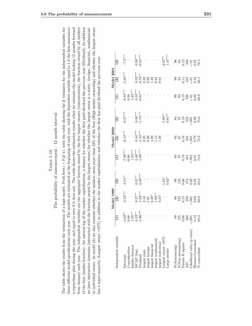
5.6 The probability of announcement 231
Table
5.1
0T
hepr
obab
ility
ofan
noun
cem
ent
-12
mon
thin
terv
al
The
table
show
sth
ere
sult
sfr
om
the
esti
mati
on
ofa
logit
model
,Pro
b(A
nn
)=
F(β
′ x),
wit
hth
eta
ble
show
ing
the
βes
tim
ate
sfo
rth
ein
dep
enden
tva
riable
sfo
r
thre
ediff
eren
tm
odel
spec
ifica
tionsea
chyea
r.T
he
model
sare
esti
mate
datth
ebeg
innin
gofea
chyea
r,w
ith
the
dep
enden
tva
riable
equalto
1if
the
firm
announce
s
are
purc
hase
pla
nduri
ng
the
yea
r,and
equalto
zero
ifit
does
not.
The
table
show
sth
ees
tim
ati
on
resu
lts
when
we
esti
mate
the
model
lookin
g12
month
sfo
rward
from
January
each
yea
r.T
he
indep
enden
tva
riable
sare
the
aggre
gate
fract
ion
owned
by
the
five
larg
est
owner
s(c
once
ntr
ati
on),
the
fract
ion
owned
by
all
insi
der
s
ofth
efirm
(insi
der
fract
ion),
the
natu
rallo
gofth
em
ark
etca
pit
aliza
tion,a
dum
my
for
whet
her
the
firm
paid
div
iden
dth
epre
vio
us
yea
r(D
ivid
end).
Inaddit
ion
we
hav
ein
tera
ctiv
edum
mie
s(i
nte
ract
edw
ith
the
fract
ion
owned
by
the
larg
est
owner
)fo
rw
het
her
the
larg
est
owner
isa
state
-,fo
reig
n-,
financi
al-,nonfinanci
al-
or
indiv
idualow
ner
.In
model
(3)
we
als
oex
am
ine
whet
her
the
insi
der
sow
ns
more
than
33%
ofth
efirm
(Hig
hin
sider
owner
ship
)and
whet
her
the
larg
est
owner
has
asu
per
-majo
rity
(Larg
est
owner
>67%
)in
addit
ion
toth
em
ark
etca
pit
aliza
tion
and
whet
her
the
firm
has
paid
div
iden
dth
epre
vio
us
yea
r.
Model1999
Model2000
Model2001
Indep
enden
tvari
able
(1)
(2)
(3)
(1)
(2)
(3)
(1)
(2)
(3)
Inte
rcep
t-4
.82∗∗
-5.5
3∗∗∗
-4.1
3∗∗
-7.9
9∗∗∗
-8.1
3∗∗∗
-8.4
7∗∗∗
-6.3
4∗∗∗
-5.6
3∗∗∗
-7.2∗∗∗
Conce
ntr
ation
0.6
8·
·-0
.98
··
0.3
8·
·In
sider
fract
ion
1.0
5∗∗
··
1.5
3∗∗∗
··
1.8
3∗∗∗
··
MC
AP
(log)
0.2
3∗∗
0.2
7∗∗
0.2
1∗∗
0.4
6∗∗∗
0.4
4∗∗∗
0.4
6∗∗∗
0.3
2∗∗∗
0.3
2∗∗∗
0.3
8∗∗∗
Div
iden
d-1
.06∗∗∗
-1.0
4∗∗∗
-0.8
8∗∗∗
-1.6
8∗∗∗
-1.7
4∗∗∗
-1.7
4∗∗∗
-0.8
1∗∗
-0.7
4∗∗
-0.9
1∗∗∗
larg
est
state
·2.1
8·
·0.2
5·
·0.2
3·
larg
est
fore
ign
·-1
.61
··
0.2
6·
·2.9
9·
larg
est
financi
al
·6.2
8∗
··
4.8
8·
·1.3
6·
larg
est
nonfinanci
al
·1.6
9∗∗
··
1.1
4·
·0.3
4·
larg
est
indiv
idual
·4.2
5∗
··
1.2
6·
·0.6
1·
Larg
est
ow
ner
>67%
··
-1.6
4∗
··
-1.8
0∗∗
··
-2.6
7∗∗
Larg
ein
sider
··
0.6
2∗
··
0.8
1∗∗
··
1.4
7∗∗∗
N(A
nnounci
ng)
80
80
80
84
84
84
96
96
96
N(N
on
announci
ng)
125
125
125
97
97
97
84
84
84
Pse
udo
Rsq
uare
0.0
60.1
30.0
60.1
80.1
60.1
90.1
30.1
10.1
2A
IC269
259
272
221
231
222
236
247
238
Lik
elih
ood
rati
o(p
valu
e)<
.001
<.0
01
0.0
2<
.001
<.0
01
<.0
01
<.0
1<
.01
<.0
1H
osm
er/Lem
eshow
0.1
30.0
30.3
50.9
10.7
90.9
00.0
20.3
40.0
5%
conco
rdant
64.2
68.0
63.3
74.8
73.2
75.6
69.8
68.1
70.5
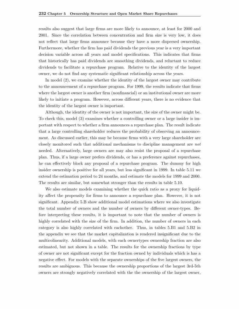
232 Chapter 5 Ownership Structure and Open Market Share Repurchases
results also suggest that large firms are more likely to announce, at least for 2000 and2001. Since the correlation between concentration and firm size is very low, it doesnot reflect that large firms announce because they have a more dispersed ownership.Furthermore, whether the firm has paid dividends the previous year is a very importantdecision variable across all years and model specifications. This indicates that firmsthat historically has paid dividends are smoothing dividends, and reluctant to reducedividends to facilitate a repurchase program. Relative to the identity of the largestowner, we do not find any systematic significant relationship across the years.
In model (2), we examine whether the identity of the largest owner may contributeto the announcement of a repurchase program. For 1999, the results indicate that firmswhere the largest owner is another firm (nonfinancial) or an institutional owner are morelikely to initiate a program. However, across different years, there is no evidence thatthe identity of the largest owner is important.
Although, the identity of the owner is not important, the size of the owner might be.To check this, model (3) examines whether a controlling owner or a large insider is im-portant with respect to whether a firm announces a repurchase plan. The result indicatethat a large controlling shareholder reduces the probability of observing an announce-ment. As discussed earlier, this may be because firms with a very large shareholder areclosely monitored such that additional mechanisms to discipline management are notneeded. Alternatively, large owners are may also resist the proposal of a repurchaseplan. Thus, if a large owner prefers dividends, or has a preference against repurchases,he can effectively block any proposal of a repurchase program. The dummy for highinsider ownership is positive for all years, but less significant in 1999. In table 5.11 weextend the estimation period to 24 months, and estimate the models for 1999 and 2000.The results are similar, but somewhat stronger than the results in table 5.10.
We also estimate models examining whether the quick ratio as a proxy for liquid-ity affect the propensity for firms to announce a repurchase plan. However, it is notsignificant. Appendix 5.B show additional model estimations where we also investigatethe total number of owners and the number of owners by different owner-types. Be-fore interpreting these results, it is important to note that the number of owners ishighly correlated with the size of the firm. In addition, the number of owners in eachcategory is also highly correlated with eachother. Thus, in tables 5.B1 and 5.B2 inthe appendix we see that the market capitalization is rendered insignificant due to themulticolinearity. Additional models, with each ownertypes ownership fraction are alsoestimated, but not shown in a table. The results for the ownership fractions by typeof owner are not significant except for the fraction owned by individuals which is has anegative effect. For models with the separate ownerships of the five largest owners, theresults are ambiguous. This because the ownership proportions of the largest 3rd-5thowners are strongly negatively correlated with the the ownership of the largest owner,
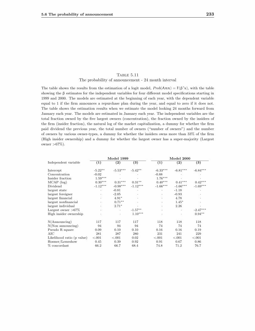
5.6 The probability of announcement 233
Table 5.11The probability of announcement - 24 month interval
The table shows the results from the estimation of a logit model, Prob(Ann) = F(β ′x), with the table
showing the β estimates for the independent variables for four different model specifications starting in
1999 and 2000. The models are estimated at the beginning of each year, with the dependent variable
equal to 1 if the firm announces a repurchase plan during the year, and equal to zero if it does not.
The table shows the estimation results when we estimate the model looking 24 months forward from
January each year. The models are estimated in January each year. The independent variables are the
total fraction owned by the five largest owners (concentration), the fraction owned by the insiders of
the firm (insider fraction), the natural log of the market capitalization, a dummy for whether the firm
paid dividend the previous year, the total number of owners (“number of owners”) and the number
of owners by various owner-types, a dummy for whether the insiders owns more than 33% of the firm
(High insider ownership) and a dummy for whether the largest owner has a super-majority (Largest
owner >67%).
Model 1999 Model 2000Independent variable (1) (2) (3) (1) (2) (3)
Intercept -5.22∗∗ -5.53∗∗∗ -5.42∗∗ -6.33∗∗∗ -6.81∗∗∗ -6.84∗∗∗
Concentration -0.02 · · -0.88 · ·Insider fraction 1.59∗∗∗ · · 1.76∗∗∗ · ·MCAP (log) 0.30∗∗∗ 0.31∗∗∗ 0.31∗∗ 0.40∗∗∗ 0.41∗∗∗ 0.42∗∗∗
Dividend -1.12∗∗∗ -0.98∗∗∗ -1.12∗∗∗ -1.66∗∗∗ -1.66∗∗∗ -1.69∗∗∗
largest state · -0.81 · · -1.18 ·largest foreigner · -2.05 · · -0.93 ·largest financial · 4.91∗ · · 4.78 ·largest nonfinancial · 0.71∗∗ · · 1.45∗ ·largest individual · 2.71∗ · · 2.26 ·Largest owner >67% · · -1.57∗∗ · · -2.47∗∗∗
High insider ownership · · 1.10∗∗∗ · · 0.94∗∗
N(Announcing) 117 117 117 118 118 118N(Non announcing) 94 94 94 74 74 74Pseudo R square 0.09 0.10 0.10 0.16 0.16 0.19AIC 281 287 280 231 241 229Likelihood ratio (p value) <.001 <.001 0.02 <.001 <.001 <.001Hosmer/Lemeshow 0.45 0.39 0.92 0.91 0.67 0.86% concordant 66.2 66.7 68.4 74.8 71.2 76.7
234 Chapter 5 Ownership Structure and Open Market Share Repurchases
and positively correlated with eachother. However, when estimating separate models,we find that the ownership of the largest owner has a negative effect on the propensityto initiate a repurchase program, consistent with the result for the dummy variable forthe controlling shareholder in table 5.10.
One thing to note about the estimations is that we do not remove firms that haspreviously announced a repurchase plan. Since several of the variables are highly per-sistent, firms that are more likely to announce every year, will be included in the modelestimation every year. To study the effect of this, we also estimate models where allfirms that has announced in previous years are removed from the sample. For example,when estimating the model for 2000, we remove all firms that announced before 2000.Although the results for 1999 remains the same, the results for 2000 becomes weakerwhile the estimation in 2001 is problematic since we are left with very few firms in bothcategories. However, it is not obvious that we should remove firms that has announcedthe previous year since it is the characteristics of these firms that we are interested in.
To summarize, the results from the model estimations above is not supportive ofan agency story where firms initiate a repurchase program to mitigate agency prob-lems. Although announcing firms have more shareholders, and a lower concentrationon average, other variables seem more important in explaining the propensity for firmsto initiate a repurchase program. The variables that are the most important decisionvariables are the previous dividend history of the firm, the insider ownership, and theexistence of a large, controlling, shareholder. Another interesting finding is that theidentity of the largest owner, or the identity of owners in general, is not important forthe decision to initiate a repurchase program.
Although these findings may be interpreted in several ways, the results are in linewith models where insiders have incentives to support a repurchase program to maximizetheir future wealth when they have a stake in the company (Isagawa, 2000), expropriateoutside shareholders or to entrench themselves and reduce the probability of takeovers.On the other hand this interpretation is not unambiguous as the existence of a con-trolling shareholder decreases the probability of announcement. This is the opposite ofwhat is the prediction in the model by Brennan and Thakor (1990). One implicationfrom their model is that large shareholders will prefer repurchases to dividends, whilesmall shareholders will prefer dividends. Our results instead suggest that controllingshareholders oppose repurchases or that additional mechanisms for distributing excesscash is not needed when a large shareholder is in place to monitor the management.
5.7 Conclusion
This study provide a detailed examination of the ownership in Norwegian firms thatinitiates repurchase programs. The main motivation is that a repurchase is an important
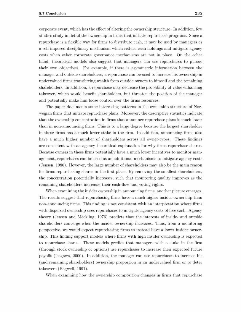
5.7 Conclusion 235
corporate event, which has the effect of altering the ownership structure. In addition, fewstudies study in detail the ownership in firms that initiate repurchase programs. Since arepurchase is a flexible way for firms to distribute cash, it may be used by managers asa self imposed disciplinary mechanism which reduce cash holdings and mitigate agencycosts when other corporate governance mechanisms are not in place. On the otherhand, theoretical models also suggest that managers can use repurchases to pursuetheir own objectives. For example, if there is asymmetric information between themanager and outside shareholders, a repurchase can be used to increase his ownership inundervalued firms transferring wealth from outside owners to himself and the remainingshareholders. In addition, a repurchase may decrease the probability of value enhancingtakeovers which would benefit shareholders, but threaten the position of the managerand potentially make him loose control over the firms resources.
The paper documents some interesting patterns in the ownership structure of Nor-wegian firms that initiate repurchase plans. Moreover, the descriptive statistics indicatethat the ownership concentration in firms that announce repurchase plans is much lowerthan in non-announcing firms. This is to a large degree because the largest shareholderin these firms has a much lower stake in the firm. In addition, announcing firms alsohave a much higher number of shareholders across all owner-types. These findingsare consistent with an agency theoretical explanation for why firms repurchase shares.Because owners in these firms potentially have a much lower incentives to monitor man-agement, repurchases can be used as an additional mechanisms to mitigate agency costs(Jensen, 1986). However, the large number of shareholders may also be the main reasonfor firms repurchasing shares in the first place. By removing the smallest shareholders,the concentration potentially increases, such that monitoring quality improves as theremaining shareholders increases their cash-flow and voting rights.
When examining the insider ownership in announcing firms, another picture emerges.The results suggest that repurchasing firms have a much higher insider ownership thannon-announcing firms. This finding is not consistent with an interpretation where firmswith dispersed ownership uses repurchases to mitigate agency costs of free cash. Agencytheory (Jensen and Meckling, 1976) predicts that the interests of inside- and outsideshareholders converge when the insider ownership increases. Thus, from a monitoringperspective, we would expect repurchasing firms to instead have a lower insider owner-ship. This finding support models where firms with high insider ownership is expectedto repurchase shares. These models predict that managers with a stake in the firm(through stock ownership or options) use repurchases to increase their expected futurepayoffs (Isagawa, 2000). In addition, the manager can use repurchases to increase his(and remaining shareholders) ownership proportion in an undervalued firm or to detertakeovers (Bagwell, 1991).
When examining how the ownership composition changes in firms that repurchase

236 Chapter 5 Ownership Structure and Open Market Share Repurchases
shares, we find that the concentration increases as would be expected. This increase inconcentration, seem to be mainly driven by an increased ownership of the largest owner.In addition, the fraction owned by institutions and personal investors decreases. Thismay both be because these investors trade more actively than the other owner typessuch that they have a higher probability of selling shares back to the firm. Alternativelythey may have a preference for dividends, making them reduce their ownership in firmsthat substitute dividends for repurchases.
The paper also examines whether ownership variables can be used to say somethingabout firms propensity to initiate a repurchase program. This is done by estimatinga binary model for the probability of observing a firm announcing a program duringeach year, given the ownership composition at the beginning of the year. The resultsreflect to a large degree the findings in the descriptive analysis. Moreover, the findingswould be in line with models where insiders have incentives to support the initiationof a repurchase program either to maximize the future value of their wealth (Isagawa,2000), expropriate outside shareholders or to entrench themselves.
On the other hand the finding that the existence of a controlling shareholder de-creases the probability of observing the introduction of a repurchase program. Thereare several interpretations for this finding. One is that a controlling shareholder mayoppose a repurchase program. Alternatively, additional mechanisms for distributingexcess cash is not needed when a large shareholder is in place with strong incentives tomonitor the management. Interestingly, this finding is the opposite of what is the pre-diction in the model by Brennan and Thakor (1990). In their model, large shareholdersprefer repurchases to dividends, while small shareholders has a preference for dividends.With respect to the identity of the largest owner in general, we find no evidence thatthe type of this owner is important for the decision to initiate a repurchase program.Finally, the results also strongly suggest that firms that paid dividends in the previousyear are less likely to initiate a repurchase program. This is likely related to dividendsmoothing, and that firms are reluctant to cutting dividends as suggested in studies byLintner (1956) and Brav et al. (2003).

5.A The probability of observing an announcement 237
5.A The probability of observing an announcement
At a general level, the model for the probability of announcement (Ann) can be writtenas,
Prob(Ann) = F(β ′x) (.2)
where β ′x is the index function, with x as a matrix of explanatory variables for eachfirm, β is a vector of coefficients and F(·) is the cumulative distribution function. Themodel is estimated as a binary regression model by assuming that a variable Ann∈ {1, 0},which is the event of a firm announcing a repurchase plan or not, is related to a set ofexplanatory variables x. A linear combination of these variables constitute an index A∗
which is related to Ann in the following way,
A∗ = β ′x + εi = β0 + β1xi1 + β2xi2 + .... + βkxik + εi (.3)
and Ann = 1 if A∗ > 0 (.4)
Ann = 0 if A∗ ≤ 0 (.5)
where β ′x is the index function, and the error term εi has a logistic or normal distri-bution with mean 0 and variance 1. Finally, we can write the probability that Ann= 1,the probability of observing the announcement of a repurchase plan during the next M
months, as,
Prob(Ann) = Prob(A∗ > 0) = Prob(β ′x) > 0 = Prob(εi > −β ′x) (.6)
Since both the normal and logistic distributions are symmetric, this can be expressedas,
Prob(Ann) = Prob(A∗ > 0) = Prob(ε < β ′x) = F(β ′x) (.7)
where F(·) defines the cumulative distribution function for ε. If F(·) is assumed to be alogistic distribution, the model is referred to as a logistic model, and if assumed to bethe normal distribution, the model is referred to as a probit model.

238 Chapter 5 Ownership Structure and Open Market Share Repurchases
5.B Additional estimation results

5.B Additional estimation results 239
Table
5.B
1T
hepr
obab
ility
ofan
noun
cem
ent
(num
ber
ofow
ners
)-
12m
onth
inte
rval
The
table
show
sth
ere
sult
sfr
om
the
esti
mati
on
ofa
logit
model
,Pro
b(A
nn
)=
F(β
′ x),
wit
hth
eta
ble
show
ing
the
βes
tim
ate
sfo
rth
ein
dep
enden
tva
riable
sfo
r
four
diff
eren
tm
odel
spec
ifica
tions
each
yea
r.T
he
model
sare
esti
mate
dat
the
beg
innin
gofea
chyea
r,w
ith
the
dep
enden
tva
riable
equalto
1if
the
firm
announce
s
are
purc
hase
pla
nduri
ng
the
yea
r,and
equalto
zero
ifit
do
not.
The
table
show
sth
ees
tim
ati
on
resu
lts
when
we
esti
mate
the
model
lookin
g12
month
sfo
rward
from
January
each
yea
r.T
he
model
sare
esti
mate
din
January
each
yea
r.T
he
indep
enden
tva
riable
sare
the
tota
lfr
act
ion
owned
by
the
five
larg
est
owner
s
(conce
ntr
ati
on),
the
fract
ion
owned
by
the
insi
der
softh
efirm
(insi
der
fract
ion),
the
natu
rallo
gofth
em
ark
etca
pit
aliza
tion,a
dum
my
for
whet
her
the
firm
paid
div
iden
dth
epre
vio
us
yea
r,th
eto
talnum
ber
ofow
ner
s(“
num
ber
ofow
ner
s”)
and
the
num
ber
ofow
ner
sby
vari
ous
owner
-types
,a
dum
my
for
whet
her
the
insi
der
s
owns
more
than
33%
ofth
efirm
(Hig
hin
sider
owner
ship
)and
adum
my
for
whet
her
the
larg
est
owner
has
asu
per
-majo
rity
(Larg
est
owner
>67%
).[w
idth
=0.5
]
Model1999
Model2000
Model2001
Indep
enden
t(1
)(2
)(3
)(1
)(2
)(3
)(1
)(2
)(3
)vari
able
Inte
rcep
t-4
.65∗∗
-0.8
4-1
.66
-8.1
6∗∗
-7.7
7∗∗
-7.4
3∗
-6.3
5∗∗∗
-4.1
0-3
.54
Conce
ntr
ation
0.9
6·
0.9
0-0
.47
·-1
.21
0.1
9·
0.6
3In
sider
fract
ion
0.9
8∗
·0.9
5∗
1.4
4∗∗∗
·1.3
1∗∗
1.8
5∗∗∗
·1.6
7∗∗∗
MC
AP
(log)
0.1
6-0
.04
-0.0
20.3
9∗∗∗
0.3
8∗∗
0.3
9∗∗
0.3
6∗∗∗
0.2
50.1
6D
ivid
end
-1.1
0∗∗∗
-0.6
9∗∗∗
-0.9
4∗∗∗
-1.6
5∗∗∗
-1.5
9∗∗∗
-1.5
2∗∗∗
-0.8
4∗∗∗
-0.5
6-0
.66∗∗
Num
ber
ofow
ner
s0.1
4·
·0.1
8·
·-0
.08
··
Sta
teow
ner
s·
-0.1
8-0
.09
·-0
.30
-0.2
1·
-0.2
3-0
.10
Fore
ign
ow
ner
s·
0.3
9∗∗
0.3
2∗
·0.4
5∗∗
0.4
8∗∗
·0.3
2∗
0.2
0Fin
anci
alow
ner
s·
-0.0
7-0
.04
·-0
.20
-0.3
0·
0.0
90.2
4N
onfinanci
alow
ner
s·
0.6
00.6
1∗∗
·0.1
30.1
3·
0.1
50.1
6In
div
idualow
ner
s·
-0.3
4-0
.33
·-0
.05
-0.0
9·
-0.3
6-0
.29
N(A
nnounci
ng)
80
80
80
84
84
84
96
96
96
N(N
on
announci
ng)
125
125
125
97
97
97
84
84
84
Pse
udo
Rsq
uare
0.0
70.0
90.1
00.1
90.1
90.2
10.1
30.1
10.1
4A
IC270
272
270
221
228
224
236
247
242
Lik
elih
ood
ratio
(pvalu
e)0.0
10.0
10.0
1<
.01
<.0
1<
.01
<.0
1<
.01
<.0
1H
osm
er/Lem
eshow
0.4
70.9
90.3
50.7
80.7
60.5
30.0
20.3
40.0
3%
conco
rdant
64.5
67.1
68.2
75.2
075.1
76.5
69.8
68.1
69.2
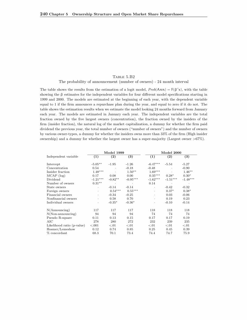
240 Chapter 5 Ownership Structure and Open Market Share Repurchases
Table 5.B2The probability of announcement (number of owners) - 24 month interval
The table shows the results from the estimation of a logit model, Prob(Ann) = F(β ′x), with the table
showing the β estimates for the independent variables for four different model specifications starting in
1999 and 2000. The models are estimated at the beginning of each year, with the dependent variable
equal to 1 if the firm announces a repurchase plan during the year, and equal to zero if it do not. The
table shows the estimation results when we estimate the model looking 24 months forward from January
each year. The models are estimated in January each year. The independent variables are the total
fraction owned by the five largest owners (concentration), the fraction owned by the insiders of the
firm (insider fraction), the natural log of the market capitalization, a dummy for whether the firm paid
dividend the previous year, the total number of owners (“number of owners”) and the number of owners
by various owner-types, a dummy for whether the insiders owns more than 33% of the firm (High insider
ownership) and a dummy for whether the largest owner has a super-majority (Largest owner >67%).
Model 1999 Model 2000Independent variable (1) (2) (3) (1) (2) (3)
Intercept -5.05∗∗ -1.95 -1.26 -6.47∗∗∗ -5.54 -5.27Concentration 0.54 · -0.18 -0.48 · -0.90Insider fraction 1.48∗∗∗ · 1.50∗∗ 1.69∗∗∗ · 1.46∗∗
MCAP (log) 0.17 0.08 0.00 0.35∗∗∗ 0.28∗ 0.30∗
Dividend -1.21∗∗∗ -0.82∗∗ -0.95∗∗∗ -1.62∗∗∗ -1.51∗∗∗ -1.48∗∗∗
Number of owners 0.31∗∗ · · 0.14 · ·State owners · -0.14 -0.14 · -0.42 -0.32Foreign owners · 0.54∗∗∗ 0.55∗∗∗ · 0.37∗ 0.38∗
Financial owners · -0.34 -0.25 · 0.03 -0.06Nonfinancial owners · 0.58 0.70 · 0.19 0.23Individual owners · -0.35∗ -0.36∗ · -0.10 -0.14
N(Announcing) 117 117 117 118 118 118N(Non-announcing) 94 94 94 74 74 74Pseudo R-square 0.11 0.13 0.15 0.17 0.17 0.19AIC 278 280 272 232 239 235Likelihood ratio (p-value) <.001 <.01 <.01 <.01 <.01 <.01Hosmer/Lemeshow 0.12 0.74 0.85 0.25 0.45 0.39% concordant 68.3 70.1 73.4 74.4 74.7 75.9

BIBLIOGRAPHY 241
Bibliography
Asquith, P. and Mullins, D. W. (1983). The impact of initiating dividend payments onsharholders’ wealth. Journal of Business, 56:77–96.
Bagnoli, M. and Lipman, B. I. (1989). Stock repurchases as a takeover defense. Reviewof Financial Studies, 2:423–443.
Bagwell, L. (1991). Share repurchases and takeover deterrence. RAND Journal ofEconomics, 22:72–88.
Barclay, M. J. and Smith, C. W. (1988). Corporate payout policy. Journal of FinancialEconomics, 22:61–82.
Bens, D. A., Nagar, V., and Wong, M. H. F. (2002). Real investment implications ofemployee stock option exercises. Journal of Accounting Research, 2:359–393.
Bøhren, Ø. and Ødegaard, B. A. (2000). The ownership structure of norwegian firms:Characteristics of an outlier. Research Report Nr.13/2000.
Bøhren, Ø. and Ødegaard, B. A. (2001). Corporate governance and economic perfor-mance in norwegian listed firms. Research Report Nr.11/2001.
Bøhren, Ø. B. and Ødegaard, B. A. (2004). Patterns of corporate ownership: Insightsfrom a unique dataset. Forthcoming in Nordic Journal of Political Economy.
Brav, A., Graham, J. R., Harvey, C. R., and Michaely, R. (2003). Payout policy in the21st century. NBER Working Paper No.9657.
Brennan, M. J. and Thakor, A. V. (1990). Shareholder preferences and dividend policy.Journal of Finance, 45:993–1018.
Comment, R. and Jarrell, G. A. (1991). The relative signaling power of dutch-auctionand fixed-price tender offers and open-market share repurchases. Journal of Finance,46:1243–1271.
Constantinides, G. M. and Grundy, B. D. (1989). Optimal investment with stock re-purchase and financing as signals. Review of Financial Studies, 2:445–465.
Dann, L. Y. (1981). Common stock repurchases: An analysis of returns to bondholdersand stockholders. Journal of Financial Economics, 9:113–138.
Denis, D. J. (1990). Defensive changes in corporate payout policy: Share repurchasesand special dividends. Journal of Finance, 45:1433–1456.
Denis, D. J., Denis, D., and Sarin, A. (1994). The information content of dividendchanges: cash flow signaling, overinvestment, and dividend clienteles. Journal ofFinancial and Quantitative Analysis, 29:567–587.
Dittmar, A. K. (2000). Why do firms repurchase stock? Journal of Business, 73:331–355.
Easterbrook, F. H. (1984). Two agency-cost explanations of dividends. The AmericanEconomic Review, 74:650–659.

242 Chapter 5 Ownership Structure and Open Market Share Repurchases
Fama, E. F. and French, K. R. (2001). Dissappearing dividends: changing firm charac-teristics or lower propensity to pay? Journal of Financial Economics, 60:3–43.
Fenn, G. W. and Liang, N. (1997). Good news and bad news about share repurchases.Working Paper, Board of Governors of the Federal Reserve, Washington D.C.
Fenn, G. W. and Liang, N. (2001). Corporate payout policy and managerial stockincentives. Journal of Financial Economics, 60:45–72.
Fried, J. M. (2002). Open market repurchases: Signaling or manegerial opportunism?UC Berkeley Public Law and Legal Theory Research Paper Series, no. 64.
Ginglinger, E. and L’Her, J. (2002). Ownership structure and open market repurchasesin france. Working Paper.
Gomes, A. and Novaes, W. (2002). Sharing of control as a corporate governance mech-anism. Working Paper, Wharton School, 09-2001.
Greene, W. (2000). Econometric Analysis. Fourth Edition, Prentice Hall.
Grinstein, Y. and Michaely, R. (2001). Institutional holdings and payout policy. WorkingPaper, Cornell University.
Grullon, G. and Michaely, R. (2002). Dividends, share repurchases, and the substitutionhypothesis. Journal of Finance, 57:1649–1684.
Howe, K. M., Vogt, S., and He, J. (2003). The effect of managerial ownership on theshort- and long-run response to cash distributions. The Financial Review, 38:179–196.
Ikenberry, D., Lakonishok, J., and Vermaelen, T. (1995). Market underreaction to openmarket share repurchases. Journal of Financial Economics, 39:181–208.
Ikenberry, D., Lakonishok, J., and Vermaelen, T. (2000). Stock repurchases in canada:Performance and strategic trading. Journal of Finance, 55:2373–2397.
Isagawa, N. (2000). Open-market stock repurchase and stock price behavior when man-agement values real investment. The Financial Review, 35:95–108.
Jagannathan, M., Stephens, C. P., and Weisbach, M. S. (2000). Financial flexibility andthe choice between dividends and stock repurchases. Journal of Financial Economics,57:355–384.
Jensen, M. C. (1986). Agency costs of free cash flow, corporate finance, and takeovers.American Economic Review, 76:323–329.
Jensen, M. C. and Meckling, W. H. (1976). Theory of the firm: Managerial behavior,agency costs and capital structure. Journal of Financial Economics, 3:305–360.
Lasfer, M. A. (2000). The market valuation of share repurchases in europe. WorkingPaper, City University Business School.
Li, K. and McNally, W. J. (2002). The decision to repurchase, announcement returnsand insider holdings: A conditional event study. University of British Columbia,Working Paper UBCFIN01-2.

BIBLIOGRAPHY 243
Lie, E. and Lie, H. J. (1999). The role of personal taxes in corporate descisions: Anempirical analysis of share repurchases and dividends. Journal of Financial and Quan-titative Analysis, 34:533–552.
Lintner, J. (1956). Distribution of incomes of corporations among dividends, retainedearnings, and taxes. American Economic Review, 46:97–113.
Masulis, R. W. (1980). Stock repurchase by tender offer: An analysis of the causes ofcommon stock price changes. Journal of Finance, 35:305–319.
McNally, W. J. (1999). Open market stock repurchase signaling. Financial Management,28:55–67.
Michaely, R., Thaler, R. H., and Womack, K. (1995). Price reactions to dividendinitiations and omissions: overreaction or drift? Journal of Finance, 50:573–608.
Miller, M. and Modigliani, F. (1961). Dividend policy, growth, and the valuation ofshares. The Journal of Business, 34:411–433.
Miller, M. H. and Rock, K. (1985). Dividend policy under asymmetric information.Journal of Finance, 40:1031–1051.
Ofer, A. R. and Thakor, A. V. (1987). A theory of stock price response to alterna-tive corporate disbursement methods: Stock repurchases and dividends. Journal ofFinance, 42:365–394.
Opler, T. and Titman, S. (1996). The debt-equity choice: An analysis of issuing firms.Working Paper, Ohio State University.
Shleifer, A. and Vishny, R. W. (1986). Large shareholders and corporate control. Journalof Political Economy, 94:461–488.
Shleifer, A. and Vishny, R. W. (1997). A survey of corporate governance. Journal ofFinance, 52:737–783.
Stephens, C. P. and Weisbach, M. S. (1998). Actual share reacquisitions in open marketrepurchase programs. Journal of Finance, 53:313–333.
Stulz, R. (1988). Managerial control of voting rights: Financing policies and the marketfor corporate control. Journal of Financial Economics, 20:25–54.
Vermaelen, T. (1981). Common stock repurchases and market signaling. Journal ofFinancial Economics, 9:139–183.
Vermaelen, T. (1984). Repurchase tender offers, signaling, and managerial incentives.Journal of Financial and Quantitative Analysis, 19:163–181.