trading behaviours analysis in an artificial stock...

Journal of Finance and Accounting 2018; 6(2): 69-75 http://www.sciencepublishinggroup.com/j/jfa doi: 10.11648/j.jfa.20180602.13 ISSN: 2330-7331 (Print); ISSN: 2330-7323 (Online)

Trading Behaviours Analysis in an Artificial Stock Market

Pan Fuchen1, 2, *

, Li Lin3

1College of Science, Dalian Ocean University, Dalian, China 2College of Basic Education, Dalian University of Finance and Economics, Dalian, China 3Department of Technology, Dalian Radio and TV University, Dalian, China

Email address:

*Corresponding author

To cite this article: Pan Fuchen, Li Lin. Trading Behaviours Analysis in an Artificial Stock Market. Journal of Finance and Accounting.

Vol. 6, No. 2, 2018, pp. 69-75. doi: 10.11648/j.jfa.20180602.13

Received: March 8, 2018; Accepted: March 19, 2018; Published: May 23, 2018

Abstract: In this paper, we study trading behavior of five different populations with different trading strategies in the

framework of an artificial stock market. Insiders who know accuracy time and quantity of inflow cash enter into market and trade

with others, which increase difficulty to get more profit for non-insiders. A new clearing mechanism that matches price in order is

mentioned. Simulation results show that trading strategies yield different results. It is noticeable that insider can easily get more

profit in short time due to prior information.

Keywords: Trading Behaviours, Artificial Stock Market, Prior Information, Market Clearing

1. Introduction

The world of business is not only complex and competitive

but contains various multiple tasks. Most of the business

organizations today are using information technology (IT)

application to improve their operational efficiency, product

and service quality [1]. Over the last decade, a fairly large

literature has explored the properties of complex financial

systems. Artificial stock market (ASM) is the realization of

complex financial market. The self-adaption, evolution,

nonlinear, bounded rationality are introduced. Computer

simulation technology is used to obtain micro-interpretation

behind macroscopic heteromorphism of financial market,

creating a new field of experimental finance [2-4]. Investment

and output are affected by individual net worth in the presence

of a financial friction at the firm level [5]. Cipriani, M., &

Guarino, A. discuss a structural model of herd behavior in

financial markets [6]. Hazem Krichene and Mhamed-Ali

El-Aroui present an artificial order-driven market able to

reproduce mature and immature stock markets properties in

the case of a single traded asset, which is designed to

simulate characteristics of immature stock markets by

reproducing their stylized facts related mainly to information

asymmetry and herd behavior. [7] Tedeschi et al. study the

herding effect through a dynamic network structure: the

communication structure allows rises and falls of Gurus over

time [8]. Mizuta et al. finds that price limits, blanket short

selling regulations, and uptick rules can prevent overshoot

and make the market efficiency during a bubble collapse, but

the last two will make the market overpriced under the

normal situation [9] Xuan Zhou and Honggang Li simulate

trader behaviors and analyze the influence of the leverage

trading on liquidity, volatility and price-discovery efficiency.

Difference from the most studies, they analyze the issue by

changing the leverage ratio, instead of introducing some

short selling regulations, such as price limits, blanket short

selling regulations, and uptick rules [10]. Anand et. al.

proposed that structural changes in an economy or in

financial markets could result because of agents’ adoption of

rules that appear to be the norm in their surroundings [11]. In

another recent work proposed a model called increasing

decreasing linear neuron for high-frequency stock market

prediction [12]. Hafezi, R. et al. propose a new intelligent

model in a multi-agent framework called bat-neural network

multi-agent system (BNNMAS) to predict stock price [13].

Regarding agent-based simulations, an option market model

based on the Black–Scholes formula was studied [14]. Xu et

al. proposed an agent-based computational model to study

multiple assets with spot-futures arbitrageurs in an attempt to

reproduce the statistical properties of real Chinese markets

70 Pan Fuchen and Li Lin: Trading Behaviours Analysis in an Artificial Stock Market

[15]. In artificial stock market, both micro level investor

behavior as well as macro level stock market dynamics are

research fields that are full of unresolved research questions

and therefore enjoy a strong interest of scholars and

practitioners alike [16, 17].

It is obvious that different investors use different investing

behaviours that are, at least partially, responsible for the time

evolution of market prices. Though no agents owe

supernatural ability to forecast price, it is more timely and

accuracy to act on transaction for some agents with insider

information.

In this paper, we present a simplified model of artificial

stock market to discuss the trading behaviors of the traders.

The market consists of five types of trade populations, which

are random traders, chartist traders, contrarian traders,

fundamentalist traders, insiders. It is crucial for all investors

to obtain the prior information, which can guide their

investment strategies. In our model, insider traders play

against other traders: only insiders have the priority of

obtaining prior information, other traders are trading with

their respective trading rules.

Firstly, we describe the formation of artificial stock market

including trade populations, interaction rules, and so on.

Secondly, we present experimental results on the price process,

which provides a possible interpretation of results. The

interactions among various populations are enough to

generate these complex outcomes. In the next section, the

model will be described in detail.

2. Traders’ Population in the Artificial

Stock Market

We built an artificial stock market with autonomous agents

using simple decision rules based on imitative and

fundamentalist behavior. Traders who buy and sell a risky

asset in exchange of cash are segmented into five

population-types, depending on their respective trading

behaviour: random, chartist, contrarian, fundamentalist, and

insider. The decision-making process of each trader is

constrained by the limited financial resources and influenced

by the volatility of the market. The trading mechanism of the

ASM is based on a realistic auction-type order matching

mechanism that allows defining a demand-supply schedule.

The number of agents engaged in trading at each moment is a

small fraction of the total number of agents.

Suppose that there are N gents in the whole market,

∑=

=5

1i

iNN , where iN represents the number of each

population-type. At every discrete trading moment t , a

trader i holds an amount )t(ci of cash and an amount

)t(si of stock.

2.1. Random Traders

Random traders are characterized by very simple trading

strategies: no intelligence and random trading constrained by

limited resources and past volatility. At the beginning of the

simulation (t = 0), random traders operate in the market; each

random make decision by comparing agent Prob To Act (the

probability of placing an order) with a stochastic number

range from 0.0 to 1.0: if agent Prob To Act < a stochastic

number, do nothing; if agent Prob To Act > a stochastic

number, buy or sell randomly, the actual quantity is chosen

randomly in a range from 1 to max Order Number (the max

buying or selling quantity in each order placed by an agent)

[18].

2.2. Chartist Traders

The chartist trader is a trend follower who makes decisions

depending on the trend of past prices. The chartist trader

speculates that, if prices are rising, they will keep rising, and if

prices are falling, they will keep falling. Chartist traders

mutual effect in the market.

At each simulation step, a chartist trader places an order

with probability 0.02, who known as strategy for those who

monitor market trend for certain history referred horizon – this

method also known as moving average (MA).

Agent sells if MA value ∑−

−=

=1

`,

,̀

1)(

t

httt

t ph

hm computed with h

time horizon is larger than the price: ε+=+ttt ppp , where

)1,0(∈ε as input parameter. They will buy if the value of MA

parameter is below the price: ε−=−ttt ppp .

The quantity that each agent is to sell is decided as follows:

( ) ( )

−=+

)h(m

p)h(mtstq

t

tts (1)

The quantity that each agent is to buy is decided as follows:

( )( )

−

=

−

t

t

tt

b

p

)h(m

)h(mptc

inttq (2)

2.3. Contrarian Traders

The contrarian traders are structured simularly to the momentum traders except in their trading behaviour. A contrarian trader speculates that, if the stock price is rising, it will stop rising soon and decrease, so it is better to sell near the maximum, and vice versa. A gent sells if MA value:

∑−

−=

=1t

httt

t`,

,`p

h

1)h(m computed with h time horizon is smaller than

the price: ε+=+ttt ppp , where )1,0(∈ε as input parameter.

They will buy if the value of MA parameter is over the price:

ε−=−ttt ppp .

2.4. Fundamentalist Traders

The fundamentalist trader believes that stocks have a

fundamental value, like 1) earnings per share (EPS) and 2)

price per earnings ratio (PIE), 3) economic characteristics of

Journal of Finance and Accounting 2018; 6(1): 69-75 71

the firm’s business (ECFB). They believe that, in the long run,

the price of the stock will revert to its fundamental price.

Consequently, they sell stocks if the price is higher than

fundamental price and buy stocks in the opposite case.

In this section, we propose the BP neural network for

fundamentalist traders of stock market, and its tuning method

for improving the decision accuracy. In recent work, Xiumei

Zhang, Chi Ma, Xinmiao Yu propose a neural network model

for financial trend predicting, which is more accuracy when

compare with China’s existing institutions and financial

website is [19].

The BP neural network is made by Rumelhant and

McClelland in 1986, It is a typical multilayer feed-forward

neural network [20]. Main existence shortcomings: slow

learning speed, easy to fall into the local minimum. There is

no theoretical guidance for the selection of the number of the

hidden layer and elements. The BP neural network algorithm

mainly consists of the forward propagation of the signal and

the inverse of the error.

The BP neural network algorithm is mainly composed of

two processes, which are the forward propagation of the

signal and the reverse propagation of the error. In the forward

propagation, the input sample is passed from the input layer,

and the hidden layer is processed to the output layer after

layer by layer. If the actual output of the output layer does

not correspond to the expected output, the reverse

transmission phase of the steering error is made. The reverse

propagation of error is to output the error back to the input

layer through the hidden layer. Each layer adjusts the weight

and threshold according to the error signal, making the error

between the output and expected output of the network

gradually decrease until the accuracy requirement is met.

The structure of the three layer BP neural network is used

in this paper. Its structure is shown in Figure 1.

Figure 1. Three layer BP neural network structure.

The input of the network input layer is as follows:

(1)( ) ( ), 1,2O j X j j M= = ⋯

The number of input variables depends on the complexity

of the system. The input and output of the hidden layer of the

network are:

(2) (2) (1)

1

( )M

i ij j

j

net k Oω=

=∑

(2) (2)( ) ( ( )), 1,2iO k f net k i T= = ⋯

Where (2)

ijω the hidden layer weighted coefficient;

superscript (1), (2), (3) representing the input layer, hidden layer and output layer.

The function of the neurons of the hidden layer takes

positive and negative symmetric Sigmoid functions:

( ) tanh( )x x

x x

e ef x x

e e

−

−

−= =+

The output layer uses a linear function:

(3) (3) (2)

1

( )M

i ij j

j

net k Oω=

=∑

(3) (3)( ) *( ( ))iO k a net k b= +

Here a, b is constant.

The BP algorithm is adopted to modify the weight, and the

learning index function uses the sum of square sum of error.

If the actual output of step K is ( )dO k , the error function

of the BP network can be expressed in the following form:

(3) (3)1( ) ( ( ) ( )) ( ( ) ( ))

2

T

d dE k O k O k O k O k= − −

In this article, there are 3 input variables, including earnings

per share (EPS), price per earnings ratio (PIE) and economic

characteristics of the firm’s business (ECFB), will be used in

the buying and selling rule.

The investor's transaction based on the numerical range of

the output layer. The five transaction behaviours (STRONG

BUY (STB), BUY (B), HOLD (HD), STRONG SELL (STS),

SELL (S)) were adopted.

2.5. Insiders Traders

Insider is a trader who can get significant information in

advance. It is well known that timely and accurate information

is a crucial factor in the stock market. As a price sensitive

event, the injection of liquidity into the market has been

chosen, simulating open market operations of the central bank.

Liquidity injection yields a higher price for shares. An insider

agent, who knows in advance the date of this event, should be

able to take in profits from this piece of insider information.

At the beginning of the simulation, each insider is given

some liquidity ��0� and no shares��0�; at a given time t*,

the global amount of cash is increased and the new cash is

exchanged to security in few days. The cash inflow is

distributed to agents proportionally to their total wealth.

The insider knows the timing and magnitude of the

injection of liquidity in advance; let r denote the number of

periods by which his information is in the lead against other

market participants; The insider is inactive for t < t*- r and acts

as a fundamentalist trader knowing the new appropriate

fundamental value, p (t > t*), for t*- r ≤ t < t*. This means

that in this time period, the insider tries to convert all the cash


into stocks. For t > t*, the insider issues sell orders if the stock

price is greater than the fundamental value p (t > t*),

otherwise he/she keeps its position.

3. Market Clearing

Suppose that at time h + 1 traders have issued U buy orders and V sell orders. For each buy order, let the pair

)p,q( bu

bu , U,,2,1u ⋯= , indicate, respectively, the quantity of

stocks to buy and the associated price. For each sell order in

the same time step, let the pair )p,q( sv

sv , V,,2,1v ⋯=

denote, respectively, the quantity of stocks to sell and the associated price.

Suppose that the inequality is satisfied as follows:

,ppp bU

b2

b1 ≥≥≥ ⋯

sV

s2

s1 ppp ≤≤≤ ⋯ (3)

Define the clearing quantity of stocks:

}q,qmin{q

V

1v

sv

U

1u

bu

* ∑∑==

= (4)

We simulate real market price mechanism: if s1

b1 pp ≥ ,

trade is executed by s1

*1 pp = , }q,qmin{q s

1b1

*1 = ; if s

1b1 pp ≤ ,

trade is executed by

s1s

1b1

b1b

1s1

b1

s1*

1 pqq

qp

qq

qp

++

+= ,

}q,qmin{q s1

b1

*1 = . Similarly, we get clearing price *

ip

according to rule ahead in order. It is necessary to note that if s1

b1 qq ≤ , we compare s

1p with b2p and vice versa. This

process is operated until quantity clearing. The clearing price

computed by the system is the *ip at which the quantity

clearing is satisfied. We define the new market price at time

step 1h + , *p)1h(p =+ . Following transactions, traders’

cash and portfolio are updated. Orders that do not match the clearing price are discarded.

4. Simulating

A. Parameter setup

We can see table 1 showing the value of variables used at

the beginning of the simulations.

Table 1. Parameter value.

Parameters Value

Number of agents ( N ) 10,000

Stock owned by each agent except insiders 100

Money owned by each agent $2000

price each stock $ 10

Number of iteration 10000

Agent Prob To Act for random trader 0.2

horizon for chartist trader 20

ε 0.01

r 700

net earnings of firm 2000000

timing of injection of liquidity 1800

magnitude of injection of liquidity 1000000

B. Simulation Result

We let the market run with 10000 agents, including 3800

random traders, 2000 chartist, 2000 contrarians, 2000

fundamentalists, 200 insiders. To give an idea of the timing

involved, assume that a time step is of the order of a day. Then,

10,000 time steps correspond roughly to 40 years of market

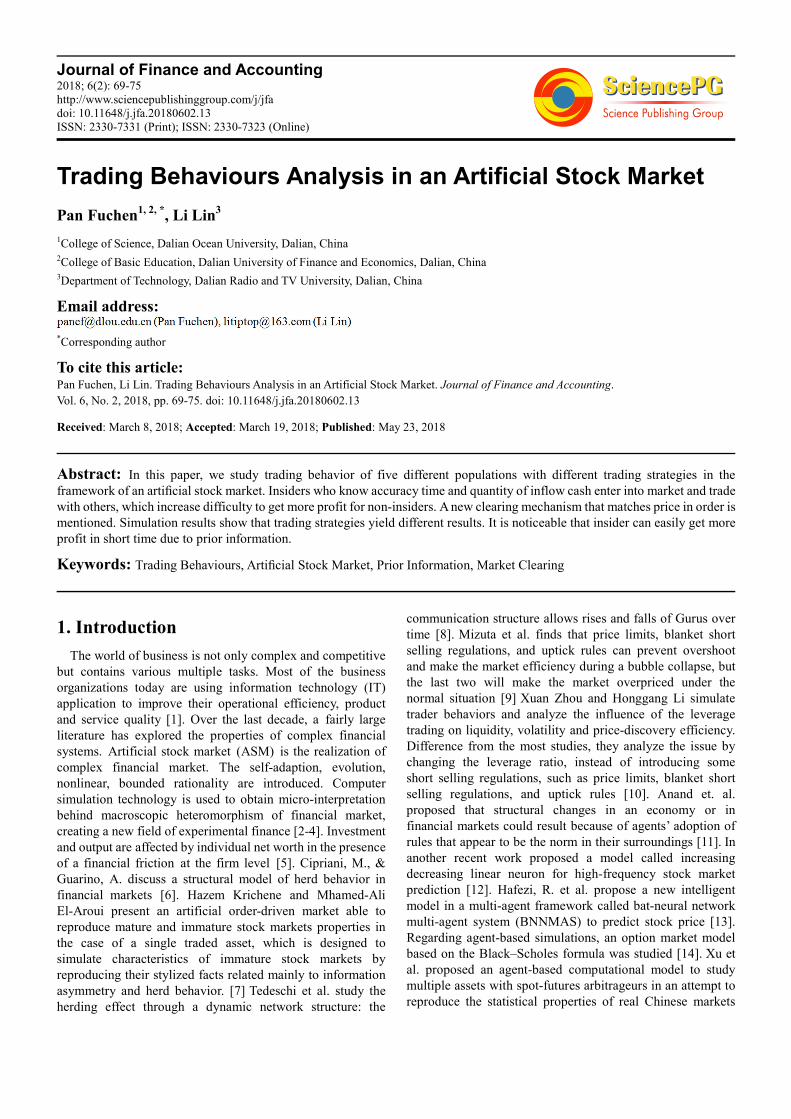
activity. Figure 2 shows the price path, and a typical simulation for

the logarithmic returns ( )

( ) log( 1)

p tr t

p t=

− can been seen from

figure 3 and figure 4. Large returns and cluster volatility are pointed out which suggest the presence of two stylized facts, i.e., fat tails and heteroscedasticity. Each population wealth curve is displayed from figure 5 to figure 9.

Figure 2. Daily time series for prices.


Figure 3. Daily time series for log returns.

Figure 4. Logarithmic returns distribution histogram.

Figure 5. Average wealth change of random traders.

Figure 6. Average wealth change of trend traders.


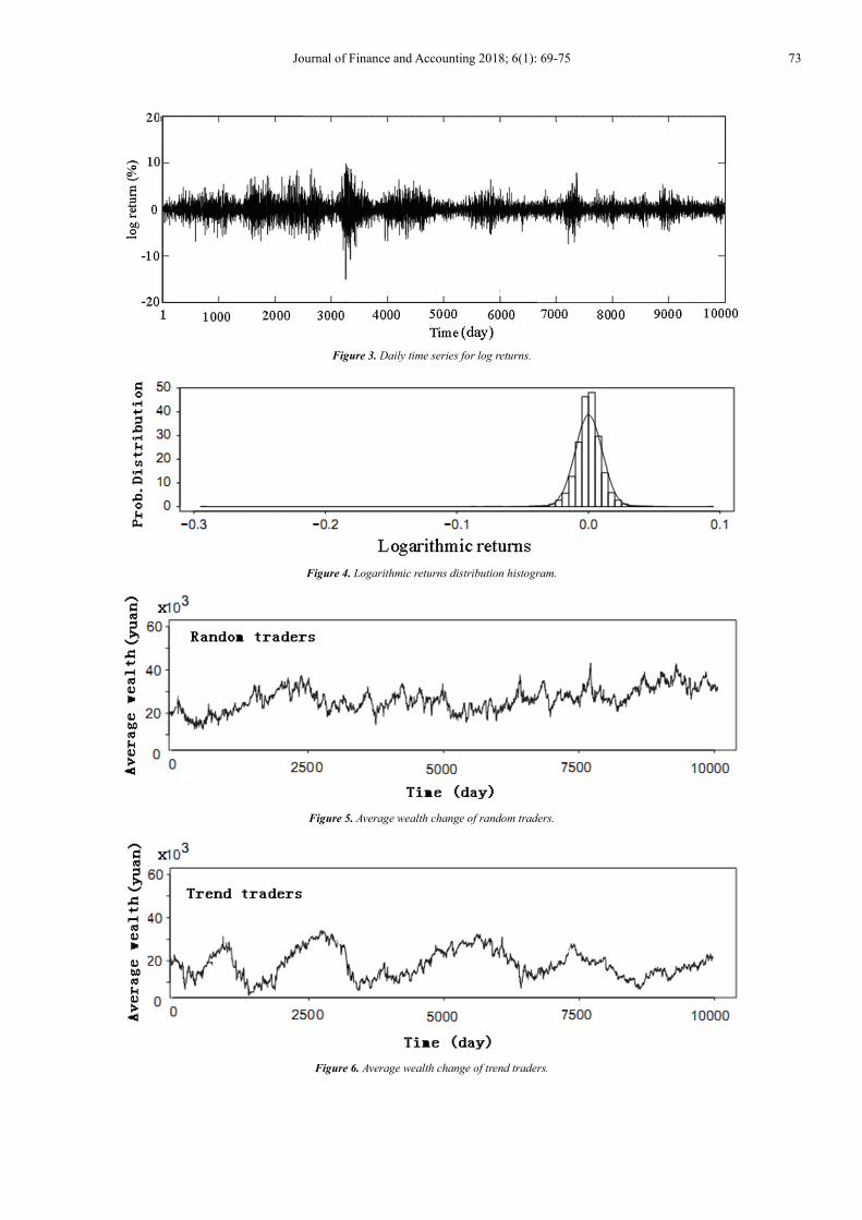
Figure 7. Average wealth change of contrarian traders.

Figure 8. Average wealth change of fundamentalist traders.

Figure 9. Average wealth change of insider traders.

See Figure 9, insiders, who know accurate timing and

quantity of cash inflow, buy stocks before information is

public and soon sell all stocks they own after information is

known and retain only cash. Thus, the change in their cash and

stock occurs because of the injection of cash. All other

populations increase their cash or stocks according to each

trading rule, but with different rates.

5. Conclusion

We discuss a simple artificial stock market with five

different populations who interact with different trading

strategies. A new clearing mechanism that matches price in

order is mentioned. Simulation results show that trading

strategies yield different results. It is noticeable that insiders

can easily get more profit in short time due to prior

information.

References

[1] John G. Mooney, V. G. a. K. L. K. A Process Oriented Framework for Assessing the Business Value of Information Technology. Forthcoming in the Proceedings of the Sixteenth Annual International Conference on Information Systems. 2001.

[2] Zhou, Qingyuan, Luo, Juan: The service quality evaluation of ecologic economy systems using simulation computing. Comput. Syst. Sci. Eng, 2016, 31 (6), pp: 453–460.


[3] Zhou, Qingyuan, Luo, Jianjian: The study on evaluation method of urban network security in the big data era. Intell. Autom. Soft Comput. 2017, DOI:10.1080/10798587.2016.1267444.

[4] Jian Yang. The artificial stock market model based on agent and scale-free network. Cluster Comput, 2017, DOI

10.1007/s10586-017-0991-4.

[5] Assenza T, Delli Gatti D, Grazzini J. Emergent dynamics of a macroeconomic agent based model with capital and credit. Journal of Economic Dynamics and Control, 2015, 50, pp:5–28.

[6] Cipriani, M., & Guarino, A.. Estimating a structural model of herd behavior in financial markets. American Economic Review, 2014, 104 (1), 224–51.

[7] Hazem Krichene· Mhamed-Ali El-Aroui, Agent-Based Simulation and Microstructure Modeling of Immature Stock Markets, Comput Econ, 2018, 51, pp:493–511, https://doi.org/10.1007/s10614-016-9615-y.

[8] Tedeschi, G., Iori, G., & Gallegati, M.. Herding effects in order driven markets: The rise and fall of gurus. Journal of Economic Behavior and Organization, 2012, 81, pp: 82–96.

[9] Mizuta, T., Izumi, K., Yagi, I., & Yoshimura, S. Investigation of price variation limits, short selling regulation, and uptick rules and their optimal design by artificial market simulations. Electronics and Communications in Japan, 2015, 98 (7), pp: 13–21.

[10] Xuan Zhou· Honggang Li, Buying on Margin and Short Selling in an Artificial, Comput Econ, 2017, DOI 10.1007/s10614-017-9722-4.

[11] Anand, K., Kirman, A., & Marsili, M.. Epidemics of rules, rational negligence and market crashes, The European Journal of Finance, 2013, 19 (5), 438–447.

[12] Arajo, RdA, Oliveira, A. L. I., Meira, S.: A hybrid model for high-frequency stock market forecasting. Expert Systems with. Applications, 2015, 42, pp: 4081–4096.

[13] Hafezi, R., Shahrabib, J., Hadavandi, E.: A bat-neural network multi-agent system (BNNMAS) for stock price prediction: case study of DAX stock price. Appl. Soft Comput. 2015, 29, pp: 196–210.

[14] Kawakubo S, Izumi K, Yoshimura S, Analysis of an option market dynamics based on a heterogeneous agent model. Intell Syst Acc Finance Manag, 2014, 21 (2), pp: 105–128.

[15] Xu HC, Zhang W, Xiong X, Zhou WX, An agent-based computational model for china’s stock market and stock index futures market. Mathematical Problems in Engineering, 2014, Article ID: 563912.

[16] Bollerslev T Generalised Autoregressive Conditional Heteroscedasticity. Journal of Econometrics, 1986, 31, pp: 307-327.

[17] Cont R. Empirical properties of asset returns: stylized facts and statistical issues. Quantitative Finance, 2001, 1, pp: 223-236.

[18] Shao Yanhua, LI Jianshi and WANG Jinghong. Model and Simulation of Stock Market Based on Agent. Proceedings of the 2008 IEEE International Conference on Information and Automation June 20-23, 2008, Zhangjiajie, China, 248-252.

[19] Xiumei Zhang, Chi Ma, Xinmiao Yu, A neural network model for financial trend predicting, Cluster Computing, 2018, https://doi.org/10.1007/s10586-018-2196-x.

[20] Wang, X., Wang, H., Wang, W. H.: Artificial neural network theory and applications. Northeastern University Press, Shenyang (2000).

trading behaviours analysis in an artificial stock...

Documents