Trade, Inequality, and the Political Economy of Institutions

Quy-Toan Do World Bank

Andrei Levchenko

International Monetary Fund

Paper presented at the Sixth Jacques Polak Annual Research Conference Hosted by the International Monetary Fund Washington, DC─November 3-4, 2005 The views expressed in this paper are those of the author(s) only, and the presence

of them, or of links to them, on the IMF website does not imply that the IMF, its Executive Board, or its management endorses or shares the views expressed in the paper.

SSIIXXTTHH JJAACCQQUUEESS PPOOLLAAKK AANNNNUUAALL RREESSEEAARRCCHH CCOONNFFEERREENNCCEE NNOOVVEEMMBBEERR 33──44,, 22000055

Trade, Inequality, and the Political Economy of Institutions∗

PRELIMINARY AND INCOMPLETE. COMMENTS WELCOME.

Quy-Toan DoThe World Bank

Andrei A. LevchenkoInternational Monetary Fund

October 2005

Abstract

We analyze the relationship between international trade and the quality of economicinstitutions, such as contract enforcement, rule of law, or property rights. The literatureon institutions has argued, both empirically and theoretically, that larger firms care lessabout good institutions and that higher inequality leads to worse institutions. Recentliterature on international trade enables us to analyze economies with heterogeneousfirms, and argues that trade opening leads to a reallocation of production in whichlargest firms grow larger, while small firms become smaller or disappear. Combiningthese two strands of literature, we build a model which has two key features. First,preferences over institutional quality differ across firms and depend on firm size. Second,institutional quality is endogenously determined in a political economy framework. Weshow that trade opening can worsen institutions when it increases the political power ofa small elite of large exporters, who prefer to maintain bad institutions. The detrimentaleffect of trade on institutions is most likely to occur when a small country captures asufficiently large share of world exports in sectors characterized by economic profits.JEL Classification Codes: F12, P48.Keywords: International Trade, Heterogeneous Firms, Political Economy, Institu-

tions.

∗We are grateful to Daron Acemoglu, Shawn Cole, Allan Drazen, Simon Johnson, Marc Melitz, MiguelMessmacher, Thierry Verdier, and participants at the World Bank workshop and BREAD conference forhelpful suggestions. We thank Anita Johnson for providing very useful references. The views expressed in thispaper are those of the authors and should not be attributed to the International Monetary Fund, the WorldBank, their Executive Boards, or their respective managements. Correspondence: International MonetaryFund, 700 19th St. NW, Washington, DC 20431. E-mail: qdo@worldbank.org; alevchenko@imf.org.

1

1 Introduction

Economic institutions, such as quality of contract enforcement, property rights, rule of law,

and the like, are increasingly viewed as key determinants of economic performance. While it

has been established that institutions are important in explaining income differences across

countries, what in turn explains those institutional differences is still an open question, both

theoretically and empirically.

In this paper we ask, how does opening to international trade affect a country’s insti-

tutions? This is an important question because it is widely hoped that greater openness

will improve institutional quality through a variety of channels, including reducing rents,

creating constituencies for reform, and inducing specialization in sectors that demand good

institutions (Johnson, Ostry and Subramanian, 2005, IMF, 2005). While trade openness

does seem to be associated with better institutions in a cross-section of countries,1 in prac-

tice, however, the relationship between institutions and trade is likely to be much more

nuanced. In the 1700’s, for example, the economies of the Caribbean were highly involved

in international trade, but trade expansion in that period coincided with emergence of slave

societies and oligarchic regimes (Engerman and Sokoloff, 2002, Rogozinski, 1999). Dur-

ing the period 1880-1930, Central American economies and politics were dominated by

large fruit-exporting companies, which destabilized the political systems of the countries

in the region as they were jockeying to install regimes most favorable to their business

interests (Woodward, 1999). In the context of oil exporting countries, Sala-i-Martin and

Subramanian (2003) argue that trade in natural resources has a negative impact on growth

through worsening institutional quality rather than Dutch disease. The common feature of

these examples is that international trade contributed to concentration of political power

in the hands of groups that were interested in setting up, or perpetuating, bad institutions.

Thus, it is important to understand under what conditions greater trade openness results

in a deterioration of institutions, rather than their improvement.

The main goal of this paper is to provide a framework rich enough to incorporate both

positive and negative effects of trade on institutions. We build a model in which institutional

quality is determined in a political economy equilibrium, and then compare outcomes in

autarky and trade. In particular, to address our main question, we bring together two

strands of the literature. The first is the theory of trade in the presence of heterogeneous

firms (Melitz, 2003, Bernard et al., 2003). This literature argues that trade opening creates

1See, for example, Ades and Di Tella (1997), Rodrik, Subramanian and Trebbi (2004), and Rigobon andRodrik (2005).

2

a separation between large firms that export, and smaller ones that do not. When countries

open to trade, the distribution of firm size becomes more unequal: the largest firms grow

larger through exporting, while smaller non-exporting firms shrink or disappear. Thus,

trade opening potentially leads to an economy dominated by a few large producers.

The second strand of the literature addresses firms’ preferences for institutional quality.

Increasingly, the view emerges that large firms are less affected by bad institutions than

small and medium size firms.2 Furthermore, larger firms may actually prefer to make

institutions worse, ceteris paribus, in order to forestall entry and decrease competition in

both goods and factor markets.3 In our model, we formalize this effect in a particularly

simple form. Finally, to connect the production structure of our model to the political

economy, we adopt the assumption that political power is positively related to economic

size: the larger the firm, the more political weight it has.

We identify two effects through which trade affects institutional quality. The first is the

foreign competition effect. The presence of foreign competition generally implies that each

firm would prefer better institutions under trade than in autarky. This is the disciplining

effect of trade similar to Levchenko (2004). The second is the political power effect. As

the largest firms become exporters and grow larger while the smaller firms shrink, political

power shifts in favor of big exporting firms. Because larger firms want institutions to be

worse, this effect acts to lower institutional quality. The political power effect drives the key

result of our paper. Trade opening can worsen institutions when it increases the political

power of a small elite of large exporters, who prefer to maintain bad institutions.

When is the political power effect stronger than the foreign competition effect? Our

comparative statics show that when a country captures only a small share of world produc-

tion in the rent-bearing industry, or if it is relatively large, the foreign competition effect

of trade predominates. Thus, while the power does shift to larger firms, these firms still

prefer to improve institutions after trade opening. On the opposite end, institutions are

most likely to deteriorate when the country is small relative to the rest of the world, but

captures a relatively large share of world trade in the rent-bearing industry. Intuitively, if

a country produces most of the world’s supply of the rent-bearing good, the foreign compe-

tition effect will be weakest. On the other hand, having a large trading partner allows the

largest exporting firms to grow unchecked relative to domestic GDP, giving them a great

2For example, Beck, Demirguc-Kunt and Maksimovic (2005) find that bad institutions have a greaternegative impact on growth of small firms than large firms.

3This view is taken, for example, by Rajan and Zingales (2003a, 2003b). These authors argue thatfinancial development languished in the interwar period and beyond partly because large corporations wantedto restrict access to external finance by smaller firms in order to reduce competition.

3

deal of political power. We believe our framework can help explain why, contrary to expec-

tations, more trade sometimes fails to have a disciplining effect and improve institutional

quality. Indeed, our comparative statics are suggestive of the experience of the Caribbean

in the 18th century, or Central America in the late 19th-early 20th: these were indeed small

economies that had much larger trading partners, and captured large shares of world trade

in their respective exports. At the end of the paper, we also support our model with a less

well-known case study: the cotton and cattle export booms in Central America between

1950 and 1980.

Our environment is a simplified version of the Melitz (2003) model of monopolistic

competition with heterogeneous producers. Firms differ in their productivity, face fixed

costs to production and foreign trade, and have some market power. If the domestic variable

profits cover the fixed costs of production, the firm enters. If the variable profits from serving

the export market are greater than the export-related fixed cost, the firm exports. Variable

profits depend on firm productivity, and thus in this economy only the most productive

firms export. Melitz (2003) shows that when a country opens, access to foreign markets

allows the most productive firms to grow to a size that would not have been possible in

autarky. At the same time, increased competition in the domestic markets reduces the size

of domestic firms and their profits. The distribution of profits thus becomes more unequal

than it was in autarky: larger firms grow larger, while smaller firms become smaller or

disappear under trade.

The institutional quality parameter in our model is the fixed cost of production. When

this cost is high, institutions are bad, and fewer firms can operate. Narrowly, this fixed cost

can be interpreted as a bureaucratic or corruption-related cost of starting and operating a

business.4 More broadly, it can be a reduced-form way of modeling any impediment to doing

business that would prevent some firms from entering or producing efficiently. For example,

it could be a cost of establishing formal property rights over land or other assets. Or, in

the Rajan and Zingales (2003a) view of the role of financial development, our institutional

quality parameter can be thought of as a prohibitive cost of external finance.

In our model, every producer has to pay the same fixed cost. We first illustrate how

preferences over institutional quality depend on firm size. We show that each producer

has an optimal level of the fixed cost, which increases with firm productivity: the larger

the firm, the worse it wants institutions to be. Why wouldn’t everyone prefer the lowest

4For example, Djankov et al. (2002) document large differences in the amount of time and money itrequires to start a business in a large sample of countries.

4

possible fixed cost? On the one hand, a higher fixed cost that a firm must pay decreases

profits one for one, and same for everyone. On the other hand, setting a higher fixed cost

prevents entry by the lowest-productivity firms, which reduces competition and increases

profits. This second effect is more pronounced the higher is a firm’s productivity. More

productive firms would thus prefer to set fixed costs higher.

As a last step in characterizing our model environment, we require a political economy

mechanism through which institutional quality is determined. The key assumption we make

here is that the larger is the size of a firm, the greater its political influence. There is a

body of evidence that individuals with higher incomes participate more in the political

process (Benabou, 2000). There is also evidence that larger firms engage more in lobbying

activity (see, for example, Bombardini, 2004). We adopt the political economy framework

of Benabou (2000), which modifies the median voter model to give wealthier agents a higher

voting weight. These ingredients are enough to characterize the autarky and trade equilibria.

Firms decide on the fixed costs of production common to all, a decision process in which

larger firms receive a larger weight. Then, production takes place and goods markets clear.

We use this framework to compare equilibrium institutions under autarky and trade, in

order to illustrate the effects of opening that we discussed above.

Our paper is closely related to several contributions to the literature on trade and insti-

tutions. In an important early work, Krueger (1974) argues that when openness to interna-

tional trade is combined with a particular form of trade policy — quantitative restrictions —

agents in the economy will compete over rents that arise from possessing a import license.

In this setting, one of the manifestations of rent seeking will be greater use of bribery and

thus corruption. Other papers have explored the effects of trade on institutions unrelated

to distortionary trade policy. For instance, Acemoglu, Johnson and Robinson (2005) argue

that in some West European countries during the period 1500-1850, Atlantic trade engen-

dered good institutions by creating a merchant class interested in establishing a system of

enforceable contracts. Thus, trade expansion affected institutions by creating a powerful

lobby for institutional improvement. Levchenko (2004) argues that trade opening changes

agents’ preferences in favor of better institutions. When bad institutions exist because they

enable some agents to extract rents, trade opening can reduce those rents. In this case,

trade leads to institutional improvement by lowering the incentive to lobby for bad institu-

tions. Our model exhibits both the foreign competition effect related to Levchenko (2004),

and the political power effect of Acemoglu et al. (2005). However, in our framework, the

more powerful groups need not favor better institutions under trade.

5

In focusing on the interaction of trade and domestic political economy, our paper is

related to Bardhan (2003) and Verdier (2005). These authors suggest that trade may shift

domestic political power in such a way as to prevent efficient or equitable redistribution.

Finally, our work is also related to the literature on the political economy dimension of the

natural resource curse. It has been argued that the presence of natural resources lowers

growth through worsening institutions. This is because competition between groups for

access to natural resource-related rents leads to voracity effects along the lines of Tornell

and Lane (1999) (see also the discussion in Isham et al., 2005).

The rest of the paper is organized as follows. Section 2 describes preferences, production

structure, and the autarky and trade equilibria. Section 3 lays out the political economy

setup and characterizes the political economy equilibria under autarky and trade. Section 4

presents the main result of the paper, which is a comparison between the autarky and trade

equilibria. We start with an analytic discussion of the conditions under which institutions

may deteriorate with trade opening. Then, we present the results of a numerical simulation

of the model, and use it discuss the comparative statics. Section 5 presents a case study, in

which we argue that the effects we identify in the model were at play in Central America in

the latter half of the 20th century. Section 6 concludes. Proofs of Propositions are collected

in the Appendix.

2 Goods and Factor Market Equilibrium

2.1 The Environment5

Consider an economy with two sectors. One of the sectors produces a homogeneous good

z, while the other sector produces a continuum of differentiated goods x(v). Consumer

preferences over the two products are defined by the utility function

U = (1− β) ln(z) +β

αln

µZv∈V

x(v)αdv

¶(1)

Utility maximization leads to the following demand functions, for a given level of total

expenditure E:

z =(1− β)E

pz

and

x(v) = Ap(v)−ε (2)

5Our notation is borrowed from Helpman, Melitz and Yeaple (2003).

6

∀v ∈ V , where ε = 1/(1−α) > 1, and we define A ≡ βE/Rv∈V p(v)1−εdv to be the demand

shift parameter that each producer takes as given.

There is one factor of production, labor (L). The homogeneous good z is produced with

a linear technology that requires one unit of L to produce one unit of z. We normalize the

price of z, and therefore the wage, to 1.

There is a fixed mass n of the differentiated goods firms, each of whom is able to

produce a unique variety of good x. Firms in this sector have heterogeneous productivity.

In particular, each firm is characterized by a marginal cost parameter a, which is the number

of units of L that the firm needs to employ in order to produce one unit of good x. Each

firm with marginal cost a is free not to produce. If it does decide to produce, it must

pay a fixed cost f common across firms, and a marginal cost equal to a. The firm then

faces a downward-sloping demand curve for its unique variety, given by (2). As is well-

known, isoelastic demand gives rise to a constant markup over marginal cost. The firm

with marginal cost a sets the price p(v) = a/α, total production at x = A¡aα

¢−ε and itsresulting profit can be written as:

π(a) = (1− α)A³ aα

´1−ε− f. (3)

The distribution of a across agents is characterized by the cumulative distribution func-

tion G(a). In order to adapt our model to a political economy framework in the later

sections, we need to obtain closed-form solutions in the goods and factor market equilib-

rium. We follow Helpman, Melitz, and Yeaple (2004) and use the Pareto distribution for

productivity. The Pareto distribution seems to approximate well the distribution of firm

size in the US economy, and delivers a closed-form solution of the model. In the Appendix,

we describe it in detail, and present solutions to the autarky and trade equilibria when G(a)

is Pareto.

2.2 Autarky

To pin down the equilibrium production structure, we need to find the cutoff level of mar-

ginal cost, aA, such that all firms above this marginal cost decide not to produce. In this

model, firm productivity takes values on the interval (0, 1b ]. The following assumption on

the parameter values ensures that the least productive firm does not operate in equilibrium,

and thus the equilibrium is interior:

f >(1− α)β [k − (ε− 1)]Lnk£1− (1− α)β ε−1

k

¤ .

7

When the equilibrium cutoff is aA, the demand shift parameter A can be written as:

A =α1−εβE

nV (aA), (4)

where we define V (y) ≡R y0 a1−εdG(a).6 The firm with productivity aA makes zero profit

in equilibrium, a condition that can be written as:

α1−εβE

nV (aA)a1−εA = f. (5)

The equilibrium value of E can be pinned down by imposing the goods market clearing

condition that expenditure must equal income:

E = L+ n

Z aA

0π(a)dG(a).

We do not have free entry in the model, that is, we have a fixed mass of producers. This

means that total income, given by the equation above, is the sum of total labor income and

the profits accruing to all firms in the economy.7 We can use (19) and (5) to write this

condition as:8

E = L− nf£aε−1A V (aA)−G(aA)

¤. (6)

The two equations (5) and (6) in two unknowns E and aA characterize the autarky

equilibrium in this economy, which we illustrate in Figure 1. On the horizontal axis is a,

which is the firm’s marginal cost parameter (thus, the most productive firms are closest

to zero). On the vertical axis is firm profit. The zero profit cutoff, aA, is defined by the

intersection of the profit curve with the horizontal axis. All firms with marginal cost higher

than aA don’t produce. For the producing firms, profit increases in productivity. Higher f

means that in equilibrium fewer firms operate: daAdf < 0. That is, the higher is f , the more

productive a firm needs to be in order to survive. Bad institutions deter entry by the less

productive agents.

6 It turns out that in the Dixit-Stiglitz framework of monopolistic competition and CES utility, the integralV (y) is useful for writing the price indices and the total profits in the economy where the distribution ofa is G(a). Each firm with productivity a sets the price of a/α. Since only firms with marginal cost belowaA operate in equilibrium, we can write the denominator of A as:

v∈V p(v)1−εdv = naA0

( aα)1−εdG(a) =

nα1−ε V (aA), leading to equation (4).

7The framework we use differs from the traditional Krugman-Melitz setup, in which there is an infinitenumber of potential entrepreneurs and free entry, and thus there are no pure profits in equilibrium. Ourchoice of keeping the mass of producers fixed is dictated by the need to adapt the model to the politicaleconomy setup. In our version of the model, all the conclusions are the same as in the more traditionalMelitz framework with free entry, when it comes to the effects of trade.

8Using the expression for profits (3), and the zero cutoff profit condition (5), we can express the profit ofa firm with marginal cost a as: π(a) = f(aε−1

A a1−ε − 1). Integrating the total profits for all a ≤ aA yieldsequation (6).

8

2.3 Trade

Suppose that there are two countries, the North (N) and the South (S), each characterized

by a production structure described above. The countries are endowed with quantities LN

and LS of labor, respectively, and populated by mass nN and nS entrepreneurs. Let fS be

the fixed cost of production in the South, and fN in the North.

Good x can be traded, but trade is subject to both fixed and per unit costs.9 In

particular, in order to export, a producer of good x must pay a fixed cost fX , and a per-

unit iceberg cost τ . We assume that these trade costs are the same for the two countries.

A firm in country i that produces a variety v faces domestic demand given by

xi(v) = Aip(v)−ε, (7)

where Ai ≡ βEi/Rvi∈V i p(v)

1−εdv is the size of domestic demand, i = N,S. Note that

the denominator aggregates prices of all varieties of x consumed in country i, including

imported foreign varieties. A firm with marginal cost a serving the domestic market in

country i maximizes profit by setting the price equal to p(v) = a/α, and its resulting

domestic profit can be written as:

πiD(a) = (1− α)Ai³ aα

´1−ε− f i, (8)

for i = N,S.

If the firm with marginal cost a decides to pay the fixed cost of exporting, its effective

marginal cost of serving the foreign market is τa, and thus it sets the foreign price equal to

τa/α, and its profit from exporting is

πiX(a) = (1− α)Aj³τaα

´1−ε− fX . (9)

where j 6= i designates the partner country, and i = N,S.

What determines whether or not a firm decides to export? A firm cannot export without

first paying the fixed cost of production f i. We also assume that τ and fX are large enough

that not all firms which find it profitable to produce domestically find it worthwhile to

export. Thus, only the higher-productivity firms end up exporting, which seems to be the

case empirically. We illustrate the partition of firms into domestic and exporting in Figure

2. The two lines plot the domestic and export profits as a function of a. As drawn, firms

with marginal cost higher than aD do not produce at all. Firms with marginal cost between

9For the sake of tractability, we assume that z can be traded costlessly. This simplifies the analysisbecause as long as both countries produce some z, wages are equalized in the two countries.

9

aX and aD produce only for the domestic market, while the rest of the firms serve both the

domestic and export markets.

To pin down the equilibrium, we must find the production cutoffs aiD, and the exporting

cutoffs aiX , for the two countries i = N,S. Similarly to the autarky case, given these cutoffs,

the size of the domestic demands in the two countries can be written as:10

Ai =α1−εβEi

niV (aiD) + njτ1−εV (ajX), (10)

where i = N,S, and j 6= i. Comparing these to the autarky demand (4), we see that the

denominators in these expressions reflect the fact that some varieties of good x consumed

in each country are imported from abroad. The cutoff values for production and export are

characterized by:(1− α)βEi

niV (aiD) + njτ1−εV (ajX)

¡aiD¢1−ε

= f i, (11)

(1− α)βEj

njV (ajD) + niτ1−εV (aiX)

¡τaiX

¢1−ε= fX , (12)

where i = N,S, and j 6= i. The model can be closed by imposing the condition that

expenditure equals income in both countries. In particular, total income is the sum of labor

income and all profits accruing to firms from selling in the domestic and export markets:

ES = LS + nSZ aSD

0πSD(a)dG(a) + nS

Z aSX

0πSX(a)dG(a)

and

EN = LN + nNZ aND

0πND(a)dG(a) + nN

Z aNX

0πNX(a)dG(a)

Using the expressions for profits in the two countries, (8) and (9), these can be rearranged

to give two equations in ES and EN :11

ES = LS + nSfS£(aSD)

ε−1V (aSD)−G(aSD)¤+ nSfX

£(aSX)

ε−1V (aSX)−G(aSX)¤

(13)

and

EN = LN + nNfN£(aND)

ε−1V (aND)−G(aND)¤+ nNfX

£(aNX)

ε−1V (aNX)−G(aNX)¤

(14)

10Each firm with productivity a serving the domestic market sets the price of a/α. Foreign firms set theprice τa/α. In the South, only firms with marginal cost below aSD operate in equilibrium, and only Northernfirms with marginal cost below aNX sell in the South, we can write the denominator of the demand shifter

AS as:vS∈V S p(v)

1−εdv = nSaSD0

( aα )1−εdG(a) + nNaNX0

( τaα )1−εdG(a) = nSα1−ε V (aSD) + nN

τα

1−εV (aSD)

using our notation.11Using the expressions for profits, (8), (9), and the zero cutoff profit conditions (11), (12), we can express

the profits of a firm with marginal cost a as: πSD(a) = f( aSDε−1

a1−ε−1) and πSX(a) = fX( aSXε−1

a1−ε−1),if it exports. Integrating the total profits yields equation (13).

10

Equations (11)-(14) determine the equilibrium values of aSD, aSX , a

ND , a

NX , E

S, and EN .

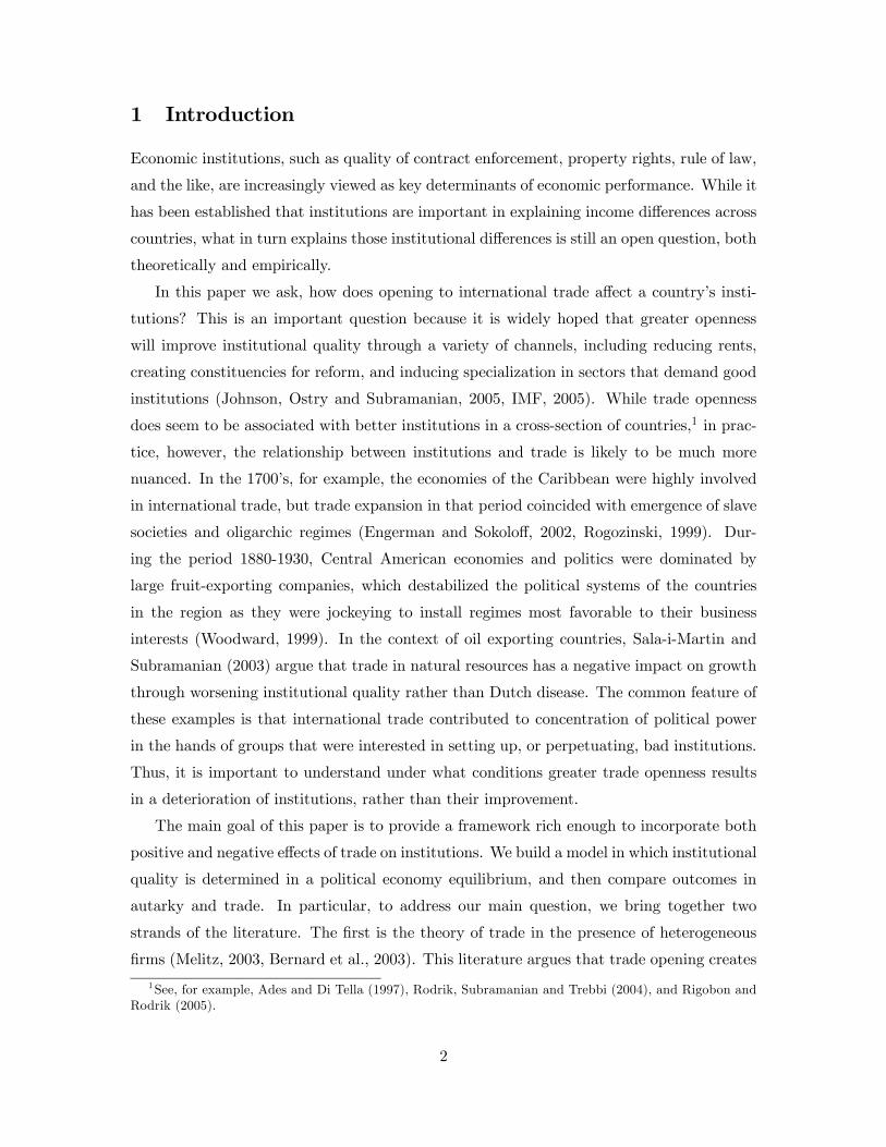
How does the trade equilibrium differ from the autarky equilibrium for given levels of f i?

For the political economy effects we wish to illustrate, the most important feature of the

trade equilibrium is that only the most productive firms export and grow as a result of

trade opening. Under certain parameter restrictions, this model has the features of the

Melitz (2003) framework which we will use in discussing how trade affects institutions. The

exact nature of the restrictions is detailed in the appendix and will be henceforth implicit.

Comparing autarky and trade, the following results hold: i) aiA ≥ aiD: higher productivity

is required to begin operating in the domestic market under trade than in autarky; ii) for

firms that operate under trade, πiD < πiA: profits from domestic sales are lower under trade

than in autarky. This implies, for instance, that firms which do not export in the trade

equilibrium face lower total profits under trade. And, iii) there exists a cutoff aiπ < aiX ,

below which a firm earns higher profits under trade than in autarky (πiD+πiX > πiA). Notice

that simply being an export firm is not sufficient to conclude that total profits increase with

trade, because of lower profits from domestic sales and fixed costs to be incurred in order

to export. Thus, when countries open to trade, the least productive firms drop out, firms

with intermediate productivity suffer a decrease in total profits, and the most productive

firms experience an increase in profit. The distribution of profits becomes more unequal

under trade.

3 Political Economy

In this paper, we think of the fixed cost of production, f , as the parameter that captures

institutional quality. It can be interpreted narrowly as a corruption cost of starting or

operating a business, or more broadly as any effect of poor institutions that acts to re-

strict entry. The quality of institutions, f , is determined endogenously through a political

economy mechanism in which entrepreneurs participate; for simplicity we abstract from the

participation of L in the political process. In order to characterize the equilibrium outcome,

we need to specify the agents’ preferences, and the political economy mechanism through

which institutional quality is determined. In our framework, preferences are equated with

agents’ wealth, and wealthier agents prefer to have worse institutions. For this, the con-

nection to the production side of the model is essential. As we show below, when a firm’s

wealth is a positively related to its profits, it is indeed the case that larger firms prefer worse

institutions.

When it comes to the political economy mechanism, the effect we would like to capture

11

is that agents with higher incomes have a higher weight in the policy decision. For instance,

Bombardini (2004) documents that larger firms are more involved in lobbying activity, and

thus we would expect them to have a higher weight in the determination of policies. Rather

than assuming a specific bargaining game, we adopt a reduced-form approach of Benabou

(2000). This approach modifies the basic median voter setup to allow for a connection

between income and the effective number of votes.

This section provides a general characterization of the political economy environment.

We state the regularity conditions that must apply in our setting, define an equilibrium,

and then prove a set of propositions showing its existence and stability. We then apply the

general results to the case in which agents’ preferences and voting weights come from the

firms’ profits in the autarky and trade equilibria. Finally, we present the main result of the

paper, which is the comparison between the autarky and trade equilibrium institutions.

3.1 The Setup

Firms participate in a political game as an outcome of which the level of barriers f ∈ [fL, fH ]is determined.12 An agent is characterized by a political weight, λ (w), which is a function

of the agent’s wealth w. We assume that the political weight function λ (w) is identical for

every agent, and takes the following form:

λ (w) = λ0 + wλ1

For a given distribution of wealth F (.), the pivotal voter is characterized by a level of

wealth wp defined by

2

Z wp

0

³λ0 + wλ1

´dF (w) =

Z +∞

0

³λ0 + wλ1

´dF (w) . (15)

We therefore assume that λ1, λ 0, and F (.) are such that:Z +∞

0

³λ0 +wλ1

´dF (w) <∞. (16)

The parameter λ1 can thus be seen as the wealth bias of the political system. Higher

values of λ1 give more political power to richer individuals, while λ1 = 0 yields the median

voter outcome, which we denote by wm. It is then straightforward to see that for every

possible political weight profile, the associated pivotal voter is always wealthier than the

median voter as long as λ1 > 0. The following Lemma establishes what kinds of pivotal

voters occur at the different levels of λ0 and λ1.12As will become clear below, we must restrict the quality of institutions, f , to a bounded interval in order

to ensure that an equilibrium exists.

12

Lemma 1 Defining by wp (λ0, λ1) the pivotal voter that prevails when the political weight

schedule is λ (w) = λ0 + wλ1, the following properties hold:

• wp (λ0, λ1) is increasing in λ1 and decreasing in λ0;

• wp (λ0, λ1) ≥ wm for any λ0 > 0, λ1 ≥ 0;

• limλ0→∞wp (λ0, λ1) = wm.¥

For the rest of the paper, we assume that wealth is derived from profits, so that for any

agent with marginal cost a ∈¡0, 1

b

¤, wealth can be expressed as wr (a, f), where r = A,T

refers to a particular regime that occurs in the economy, that is, autarky or trade. We

must put a set of regularity conditions on the function wr (a, f) in order to ensure that

the political economy equilibrium is well-behaved. We detail these conditions formally in

the Appendix. Aside from the usual assumptions about twice—continuous—differentiability

with respect to a and f , we assume that the marginal impact of an increase in f on wealth,

∂wr (a, f) /∂f is decreasing in f (concavity), but also decreasing in a: more productive

entrepreneurs suffer relatively less from higher barriers to entry than their less productive

counterparts do.

We now discuss the two ingredients necessary to find a political economy equilibrium:

we need to know the identity of the pivotal voter, given by the marginal cost a = p, and we

need to know what institutions that pivotal voter prefers. We start with the latter.

3.2 The Preference Curve

The Preference Curve is the locus of all the points (p, f) ∈¡0, 1

b

¤× [fL, fH ] such that f

is the preferred level of entry barriers of an entrepreneur with marginal cost a = p. We

denote the Preference Curve by fr (p). We make the simplifying assumption that for all

entrepreneurs, the preferred level of f is simply the one that maximizes their wealth.

Proposition 2 When regularity conditions (A.6) through (A.10) are satisfied, there exist

two thresholds f−1r (fH) and f−1

r (fL) ∈¡0, 1

b

¢, such that the Preference Curve is a well-

defined piecewise continuously differentiable mapping given by:

fr (p) =

⎧⎪⎨⎪⎩fH if p ≤ f−1

r (fH)nfr :

∂∂fwr (p, fr) = 0

oif p ∈

£f−1r (fH) , f

−1r (fL)

¤fL if p ≥ f−1

r (fL)

Furthermore, the Preference Curve fr (p) is nonincreasing almost everywhere.¥

13

The first part of the Proposition shows that when the wealth-maximizing level of f

is interior, it can be obtained simply from taking the first-order condition of wealth with

respect to f . The second part states that wealthier agents prefer worse institutions. The

non-standard assumption driving the latter result is that ∂wr (a, f) /∂f is increasing in a:

the marginal benefits of raising entry barriers must be higher for higher productivity agents.

Then, higher marginal cost entrepreneurs prefer lower levels of entry barriers, all else equal.

When the profit-maximizing level of f is not interior, the entrepreneur prefers either fH or

fL, and all entrepreneurs that are more (less) productive also prefer fH (fL).

Let us now make the connection between the goods market equilibrium outcomes under

the autarky and trade regimes and the Preference Curve. In particular, suppose that the

wealth functions take the following form:

wA (a, f) =

(πA(a,f)P (f) if a ≤ aA (f)

0 if a ≥ aA (f)(17)

in autarky, and

wT (a, f) =

⎧⎪⎨⎪⎩πD(a,f)+πX(a,f)

PS(f)if a ≤ aX (f)

πD(a,f)PS(f)

if a ∈ [aX (f) , aD (f)]0 if a ≥ aD (f)

(18)

under trade. That is, agents’ wealth is simply real profits (P (f) and PS (f) are aggregate

price levels in autarky, and in the South under trade respectively).

Corollary 3 When wr (a, f) is given by (17) or (18), it satisfies regularity conditions (A.6)

through (A.10). Thus, both autarky and trade regimes are characterized by almost every-

where downward sloping Preference Curves.¥

Why would any producer prefer to set f at any level higher than fL? The key trade-

off is that a higher level of fixed cost lowers every firm’s profits one for one. However, a

higher level of f also results in less entry. With fewer producers operating in the economy,

the active firms’ variable profits are higher. Most importantly, this second effect is more

pronounced for higher productivity firms, which implies that the more productive firms

prefer to live with worse institutions. We can rewrite the expression for autarky profits,

(3), using (4):

π(a)

P=

a1−εh

(1−α)βEnV (aA)

i− f

P, (19)

keeping in mind that P , E and aA are equilibrium values that are themselves functions of

f . The first term in the numerator is the variable profits. It is true that raising f lowers

14

the total profits, because the firm must pay higher fixed costs and entrepreneurs-consumers

face higher aggregate price. However, raising f also raises the variable profits, because it

pushes more firms out of production. In particular, V (aA) decreases with f .13 Furthermore,

variable profits are multiplicative in a1−ε, which is a term that rises and falls with the firm’s

productivity. Thus, a firm with a higher productivity will reach maximum profits at higher

levels of f .

Figures 3 and 4 illustrate this Proposition. Figure 3 reproduces Figure 1 for two different

levels of f . We can see that raising f forces the least productive firms to drop out. Further-

more, the slope of the profit line is higher in absolute value for higher f : variable profits are

higher at each productivity. Thus, firms above a certain productivity cutoff actually prefer

a higher f , as the variable profit effect is stronger than the fixed cost effect. To illustrate

this point further, Figure 4 plots the profits of two firms as a function of f . The profits

of each firm are non-monotonic in f , first increasing, then decreasing in it. A firm with a

higher productivity attains maximum profits at a higher level of f . This heterogeneity in

firm preferences over institutions is the key feature of our analysis.

In the trade equilibrium, firms’ preferences over institutional quality differ from those in

autarky. This is because the level of f in the domestic economy affects both the domestic

production and the pattern of its imports. Nonetheless, the essential trade-off remains

unchanged. On the one hand, a higher f implies higher variable profits, an effect that is

stronger for more productive firms. On the other, the higher fixed cost decreases profits

one for one. Comparing to autarky, we must keep in mind that f may also affect the firms’

decision whether or not to export, and its profits from exporting.

Having completed our description of firms’ preferences, we now move to a discussion of

the political economy mechanism.

3.3 The Political Curve

The Political Curve is defined by the set of points (p, f) ∈£0, 1

b

¤× [fL, fH ], where p is the

pivotal voter in the economy that produces with fixed cost equal to f . That is, the Political

Curve pr (f) is defined implicitly by:

2

Z p

0

hλ0 + wλ1

r (a, f)idG (a) =

Z 1/b

0

hλ0 + wλ1

r (a, f)idG (a) , (20)

when the pivotal voter thus defined is unique for every f . When λ1 = 0, the resulting

pivotal voter is actually the median voter that we denote pm.13 In practice, there is another effect, which is that as f increases E decreases also. We show in the proof

to Corollary 3 that the net effect is that raising f raises variable profits.

15

Proposition 4 When regularity conditions (A.6), (A.7), and (A.12) are satisfied, the Po-

litical Curve is a well-defined and piecewise continuously differentiable function of f . Fur-

thermore, under regularity conditions on the political weight function, the Political Curve is

downward sloping almost everywhere.¥

The first part of this Proposition formally establishes the equivalence between defining a

pivotal voter by her wealth and by her marginal cost of production. This result comes from

assumptions (A.6) and (A.12), which imply that there exists a one-to-one correspondence

between wealth and marginal cost in the neighborhood of any potential pivotal voter. We

can hence restate previous results in terms of marginal cost of production a rather than

wealth, keeping in mind that the mapping between the two is decreasing. The second part of

the Proposition takes one extra step in characterizing the Political Curve. In particular, we

would like to show that under certain conditions, the Political Curve is downward sloping.

That is, we would like to restrict attention to cases in which a higher level of fixed cost

results in a pivotal voter that is more productive. This is a sensible requirement: a higher

level of f decreases the wealth of the least productive firms, and increases the wealth of

the most productive firms, thus shifting the voting weight towards the higher productivity

firms. We illustrate this in Figure 5, which plots the densities of profits for two values of

fixed cost, fh > fh. Nonetheless, for this Proposition to hold, certain restrictions on the

function λ(w) must be satisfied: it must give enough weight to wealthier agents relative to

less wealthy ones.

3.4 Equilibrium: Definition, Existence, Characterization

We now define the equilibrium that results from the agents’ preferences and the voting. As

the discussion above makes clear, there is a two-way dependence in our setup: the identity

of the pivotal firm, p, depends on the level of f , while the level of f depends on the identity

of the pivotal firm. Our equilibrium must thus be a fixed point.

Definition 5 (Equilibrium) An equilibrium of the economy is a pair (fr, pr) such that

fr = fr (pr), and pr = pr (fr), where fr ∈ [fL, fH ] and pr ∈¡0, 1

b

¢.

Proposition 6 There exists at least one equilibrium.¥

Given our characterization of the Preference Curve and the Political Curve above, the

definition of equilibrium and its existence can be illustrated with the help of Figure 6. The

proof of this Proposition shows that one of three cases are possible: fL, fH , or an interior

16

value of f . The first two occur when the two curves intersect on the flat portion of the

Preference Curve.

Having established existence, we now would like to characterize potential equilibria. We

will not consider an explicitly dynamic setting to address issues of stability. We instead

define the following functions: ∀f ∈ [fL, fH ] ,

Φr (f) = fr [pr (f)]

and by induction, for n ≥ 1,

Φ0r (f) = f, and Φnr (f) = Φr

£Φn−1r (f)

¤. (21)

Similarly, we define for p ∈¡0, 1

b

¢,

Πr (p) = pr [fr (p)]

and for any n ≥ 1,Π0r (p) = p, and Πnr (p) = Πr

£Πn−1r (p)

¤. (22)

Definition 7 (Stability) An equilibrium (fr, pr) is stable if there exists ρ > 0, such that

for any η > 0, there exists an integer ν ≥ 1 such that for any n ≥ ν, p ∈ (pr − ρ, pr + ρ) ,

and f ∈ (fr − ρ, fr + ρ) ,

|Πnr (p)− pr| < η; (23)¯Φnr

³f´− fr

¯< η. (24)

In other words, an equilibrium will be considered stable if, after a small perturbation

(of size ρ) around the equilibrium point, the system converges back to the equilibrium, with

(21) and (22) characterizing the dynamic process. Note that for any entry barrier level f ,

fr [Πn (pr (f))] = Φ

n+1 (f), and pr [Φn (fr (p))] = Π

n+1 (p), so that by continuity of fr (.)

and pr (.), the two requirements (23) and (24) are redundant. The definition of stability

above corresponds to the concept of asymptotic stability in dynamic processes. Two generic

cases of equilibria that violate the stability requirement that might arise are: (i) a “cycling”

case, whereby the process is bounded but does not converge; (ii) the process diverges after

a perturbation and reaches a corner solution. We prove the following proposition by consid-

ering these two cases. We first argue that cycling cannot occur as Preference and Political

curves are downward sloping, and then establish that if there does not exist any stable

interior equilibrium, then one of the two corners is an equilibrium, and corner equilibria are

stable.

17

Proposition 8 There exists a stable equilibrium.¥

We can now apply the results proved in this section to the autarky and trade regimes.

When wealth equals profits, and is thus defined by (17) and (18) in autarky and trade

respectively, we have the following result:

Corollary 9 Under regularity conditions, both autarky and trade regimes are characterized

by downward sloping Preference and Political Curves. Furthermore there exists a stable

equilibrium in both autarky and trade regimes.¥

4 Institutions in Autarky and Trade

We now compare the equilibrium institutions in the South that occur under autarky and

trade. All throughout, we assume that the North’s institutions are exogenously given, and

all the adjustment in the North takes place on the production side. When an economy

opens to trade, both the Preference Curve and the Political Curve shift. We investigate the

behavior of Political and Preference Curves in turn.

4.1 The Political Power Effect

The reorganization of production due to trade opening leads the Political Curve to shift

“inwards.” In particular, at any f , the most productive firms begin exporting, and the distri-

bution of profits becomes more unequal: relative wealth shifts towards the more productive

firms. This means that the pivotal voter moves to the left, pT (f) ≤ pA(f) ∀f ∈ [fL, fH ].We label this the political power effect: the power shifts towards larger firms under trade

compared to autarky. Once again, while the notion that increased profit inequality leads the

pivotal voter to shift in this direction is intuitive, the proof depends crucially on regularity

conditions governing λ(w): the political weight function must be sufficiently increasing in

wealth.

Proposition 10 Under regularity conditions on λ(w), the Pivotal Voter curve moves in-

ward as the economy opens to trade.¥

The latter requirement states that the profits of the most productive firm (a→ 0) must

be strictly higher under trade than in autarky. We can show that it is satisfied for small

enough values of nN . A formal proof is given in the appendix.

18

4.2 The Foreign Competition Effect

We now need to make a statement about how the Preference Curve shifts. It turns out

that for most parameter values, and for values of a high enough, a firm at a given level of

a prefers to have better institutions under trade than in autarky. This very much related

to the Melitz effect, and comes from the fact that domestic profits are lower under trade

due to the increased foreign competition.14 We label this inward shift of the Preference

Curve the foreign competition effect. We must keep in mind that the most productive of

the exporting firms may actually prefer worse institutions under trade, because as we saw

above, export profits increase in f . It is also true that in principle, parameter values may

exist under which the inward shift of the Preference Curve does not occur. This would

happen, for example, is nN

nSis sufficiently low.15 When that is the case, the inward shift of

the Political Curve unambiguously predicts a worsening of institutions as a result of trade.

Otherwise, the two effects conflict with each other.

4.3 Comparing Institutions in Autarky and under Trade

In comparing the equilibria resulting under trade and autarky, we face the potential difficulty

that the trade equilibrium may note be unique. Thus we must define an equilibrium selection

process. We assume that the equilibrium resulting from trade opening is the one to whose

basin of attraction the autarky equilibrium fA belongs. To do so, we must define a basin

of attraction with respect to f .

Definition 11 The basin of attraction of a stable equilibrium (fT , pT ) is denoted B (fT )

and is defined as

B (fT ) = {f ∈ [fL, fH ] , ∀η > 0,∃ν > 1,∀n > ν, |Φn (f)− fT | < η}

We now show that there exist parameter values under which the transition from autarky

to trade implies a worsening of institutions.

Proposition 12 Consider an interior and stable autarky equilibrium (fA, pA). If pT (fA) <

f−1T (fA), then there exists an equilibrium of the economy under trade (fT , pT ) such that

fA ∈ B (fT ) and fA < fT .¥14To be more precise, the Melitz effect is about the level of profits, while the foreign competition effect is

about their derivative with respect to f . It turns out that the conditions that guarantee the Melitz effect inour model are also sufficient to generate the foreign competition effect.15 In the most extreme case, suppose that there are no producers of the differentiated good in the North:

nN = 0. Then, clearly, there is no reason for the foreign competition effect to occur, because there is noforeign competition in that sector.

19

The above Proposition shows that if the political power effect is large enough compared

to the foreign competition effect, then the economy will converge towards an equilibrium

with worsening institutions. In order to compare the foreign competition and political

power effects, let’s compare the pivotal voter under trade starting from autarky institutions,

pT (fA), and the entrepreneur who prefers fA under the trade regime, f−1T (fA). If pT (fA) <

f−1T (fA), then the political power effect is stronger than the competition effect. When is

this the case? We can consider the following difference:

∆ =

Z f−1T (fA)

0λ (wT (a, fA)) dG (a)−

Z 1/b

f−1T (fA)

λ (wT (a, fA)) dG (a)

It is positive if and only if pT (fA) < f−1T (fA).16 We can use the autarky pivotal voter to

rewrite this expression as:

∆ =

Z pA(fA)

0λ (wT (a, fA)) dG (a)−

Z 1b

pA(fA)λ (wT (a, fA)) dG (a)

−2Z pA(fA)

f−1T (fA)

λ (wT (a, fA)) dG (a)

The first part of this expression represents the magnitude of the Political Power curve shift.

It is positive, because pT (fA) < pA (fA). The second term proxies for the strength of the

foreign competition effect. It will be large in absolute value when there is a large difference

between pA (fA) and f−1T (fA): agents’ preferences change strongly between autarky and

trade. Note that if the integral of the second term is negative, ∆ > 0 unambiguously: the

two effects reinforce each other, and institutions deteriorate. When foreign competition

changes preferences in favor of better institutions, the two effects act in opposite directions.

We present the two cases graphically in Figure 7, starting from the same interior au-

tarky equilibrium. The first panel illustrates a transition to a trade equilibrium in which

institutions improve as a result of trade. For this to occur, the shift in the Political Curve

must be sufficiently small, and the shift in the Preference Curve sufficiently large. The

former would occur, for example, if the function λ(w) was flat enough. The latter would

occur if the foreign competition effect is sufficiently pronounced, that is, when nN is large

enough relative to nS . The second panel illustrates a case in which institutions deteriorate

as a result of trade. If the political power effect is strong enough, or the foreign competition

effect is weak enough, institutions will worsen.

What are the conditions under which the two different scenarios are more likely to

prevail? The model does not offer an analytical solution with which we could perform com-16Note that when pT (fA) = f−1

T (fA), ∆ = 0, as pT (fA) is the pivotal voter.

20

parative statics with pencil and paper, due to both the algebraic complexity of the trade

side of the model, and the fact that we cannot find closed-form expressions for the pivotal

firm. Nonetheless, we can implement the solution numerically in a fairly straightforward

manner. In order to focus especially on the South’s market power and the resulting mag-

nitude of the foreign competition effect, we compare changes in institutions for a grid of

parameter values. Starting from an interior autarky equilibrium, we check how it changes

in response to trade opening for a grid of LN ’s and nN ’s.17

The results are illustrated in Figure 8. It depicts ranges of LS/LN and nS/nN for which

institutions improve and deteriorate as a result of opening. The shaded area represents

parameter values under which institutions deteriorate. Trade is most likely to lead to a

deterioration when the economy is both small in size (LN is large compared to LS), and

captures a large share of world trade in the differentiated good (that is, nS is large relative

to nN). Under these conditions, there is a large movement in the pivotal voter, while the

movement in the Preference Curve is small, or can even be positive — that is, some range of

firms may want worse institutions under trade than in autarky in some cases. Intuitively,

when there are relatively few producers of the competing good in the North (nN is low),

the disciplining effect of opening up to foreign competition will be weak. On the other

hand, when the size of the foreign demand is large relative to the home labor force, the

incentive to push smaller firms out of the market in order to earn higher profits will be

higher. In addition, for those firms that do export, larger size of the foreign export market

means higher profits, ceteris paribus, and thus more political power at home. We can also

highlight the conditions under which the opposite outcome obtains: the disciplining effect

of trade predominates. When the number of domestic firms is small vis-a-vis its trading

partner, foreign competition in the domestic market forces even the biggest firms to want to

improve institutions in order to increase their profits. Thus, when domestic firms capture a

very small share of the world market under trade, the shift in the Preference Curve is large.

When this is the case, the economy is likely to retain good institutions or even improve

them. This effect is more pronounced when the South is also relatively large — the mirror

image of the previous case we analyzed. Figure 9 reports equilibrium trade institutions for

the same grid of parameter values. The darkly shaded area represents all cases under which

institutions deteriorate as a result of trade, while in the lightly shaded area institutions

improve. We can see that the nS/nN dimension matters more than the LS/LN dimension:

17We adopt the following parameter values: β = 0.5; ε = 3; k = 4; b = 0.1; LS = 1000; nS = 20;fL = (1−α)β[k−(ε−1)]L

nSk[1−(1−α)β ε−1k ]; fH = 181; τ = 1.1; fX = 150; λ0 = 1; λ1 = 0.875; fN = 48. Details of numerical

implementation and the MATLAB programs we used are available upon request.

21

institutions always worsen more sharply when raising the latter than the former. We can

also see that when the South’s market power is sufficiently high, institutions deteriorate

quite sharply.

5 Case Study: Cotton and Beef in Central America, 1950-198018

Given the intuitions that we developed in the previous sections, Central America would

seem to be a good place to look for examples of how trade opening can have deleterious

effects on institutions. Even taken as a whole, the Central American economy is a very small

one located in relative proximity to the large US market. Furthermore, these countries have

historically been characterized by policies of economic liberalism, and protectionism was

never a prominent feature of the political landscape.

While the role of large banana producers in these economies is well-known, in this case

study we illustrate the impact of export booms in cotton and beef on these economies in the

second half of twentieth century. What makes these cases especially interesting is that in

this period, export promotion was a deliberate strategy on the part of the US government

and multilateral institutions whose goal was to bring economic growth and stability to these

countries. The policies that were enacted did succeed in promoting exports, which grew at

an average rate of 10% a year between 1960 and 1970 across Central America. Economic

growth was also robust in this period.

Let us see what effect the expansion of trade had on institutions. First, we document

that the explosion of exports in these two sectors was due largely to factors outside Central

American control, such as technological progress and changes in geopolitical objectives of

the US. Then, as we go through the discussion, we will argue that key aspects of Central

American trade in this period match the salient features of our model: there are economic

profits to be made from exporting; the region captures a sizeable share of trade in the

rent-bearing good; larger producers grow larger through exporting, while smaller producers

languish; political influence is tied to wealth. Finally, the evidence would seem to suggest

that institutions did deteriorate as a result of trade, as trade opening gave the largest

producers strong incentives to expropriate the smaller ones.

18This section is based on a book by Robert Williams, entitled “Export Agriculture and the Crisis inCentral America.” (1986).

22

5.1 Cotton

5.1.1 The Natural Experiment: Factors Behind Cotton Export Explosion

The Pacific coastal plain of Central America is quite narrow, measuring between 10 and 20

miles wide, but it is characterized by rich volcanic soils ideally suitable for cotton cultivation.

The plain is relatively flat, thus permitting mechanization, and the presence of both rainy

and dry seasons implies that irrigation is not needed, while at the same time plants would

not be damaged by rain at later stages of the season. Nonetheless, cotton production in

Central America was minimal until 1950, and exports outside the region were virtually nil.

Several key factors were behind the cotton explosion after 1950. World demand for cot-

ton increased dramatically in the few years following World War II, as developed countries

enjoyed robust growth. Foreign demand combined with important technological advances.

The first was the insecticide DDT. Large scale attempts to grow cotton in Central America

had failed in the past because there had been no effective means to combat insects in the

area. That changed dramatically once DDT was invented in 1939. The second innovation

was the introduction of modern fertilizers. Finally, productivity was greatly improved by

the introduction of the tractor.

5.1.2 Export Boom and Features of the Cotton Industry

The combination of a rise in foreign demand and improvements in technology produced

growth in the cotton sector that was nothing short of spectacular. During the 1940’s, all of

Central America produced only about 25,000 bales a year, most of it for textile mills within

the region. Central American production exceeded 100,000 bales in 1952, 300,000 in 1955,

and 600,000 in 1962. At that time, the region ranked 10th in the world in cotton production.

By mid-1960’s, production rose to more than 1 million bales, and by the late 1970’s, Central

America as a whole ranked third in the world in cotton production, below only the United

States and Egypt. A key feature of this growth is that while at the beginning of the period

virtually all of the cotton production was consumed within the region, from 1955 onwards

90% of it was exported outside Central America.

What did the cotton industry look like in this period? There were around 2,000 cotton-

growing farms in Central America, and that number rose to 10,000 over the following 20

years. The average size of a cotton plot over this period was 100 acres. A closer look reveals

enormous inequality in farm size. At one extreme, there was a group of very small growers.

Across the different Central American countries, between 25 and 60% of all growers planted

an average of 5 acres of cotton on a farm of less than 25 acres. Medium-sized farmers,

23

planting an average of 20 acres, were the second-largest group.

By contrast, the overwhelming majority of land under cotton cultivation belonged to

large producers. For example, in Guatemala, farms with fewer than 122 acres made up

less than 2% of cotton-growing lands, while farms larger than 1100 acres produced 62%

of the cotton. In El Salvador, farms under 125 acres represented 82% of the growers, but

17% of cotton-growing land area. The picture is quite similar in other countries. These

figures, however, do not reveal the full extent of concentration, because often the same

family controlled multiple estates. Thus, the dispersion of firm size, which is a crucial

feature of our theory, seems to also be a prominent feature of the cotton industry in these

countries.

Available evidence indicates that the large cotton growers were none other than the

established landholding aristocracies in these countries. All in all, these were several dozen

families, who reaped the bulk of the gains from trade in cotton. Along with using land to

grow it, these family enterprises often invested in other phases of cotton production, such

as ginning, insecticide production, and credit. Besides the established landholders, there

emerged another class of growers, which was comprised of urban dwellers who saw cotton

as an investment opportunity. Coming from urban areas, these entrepreneurs nevertheless

were successful, due in large part to being politically well-connected.

5.1.3 Land Expropriation

The cotton boom of such proportions naturally involved significant growth of the land area

under cotton cultivation. While some of it came from deforestation, another major source of

new cotton lands was through eviction of small farmers. This process came in two varieties.

First, peasants were expelled from lands which were clearly titled to the landlord. Usually,

this occurred when the landlord raised the rent to levels that represented the opportunity

cost of not using the land to grow cotton. This kind of eviction was usually regarded

as benign, and did not produce much overt social conflict. Second, landlords and other

prospective cotton growers used their political power to get titles to the lands previously

owned by the national government and municipalities. According to Williams, “[u]ntitled

lands lying near proposed roadways were quickly titled and brought under the control of

cotton growers or others with privileged access to the land-titling institutions in the capital

city.” (Williams, 1986, p. 56). Once the land was titled in this manner, peasants cultivating

this land were promptly evicted.

Some lands were owned by a municipality and cultivated by the peasants for a nominal

24

fee. This was called the “ejidal” system, and represented something akin to communal own-

ership of land by peasants. Since in this case, the legal status of the lands was more clear

than when the lands were untitled, more effort was required to expropriate them. Neverthe-

less, “[w]here ejidal forms came in the path of the cottonfields, the rights were transferred

from municipalities to private landlords through all sorts of trickery and manipulation.”

(Williams, 1986, p. 56).

In summary, the remarkable growth in export opportunities both increased the political

power of the largest producers, and provided them with a strong incentive to push smaller

producers out. The result was a wave of land expropriations, consistent with the effect we

are illustrating in our model.

5.2 Beef

5.2.1 The Natural Experiment: Factors Behind Beef Export Explosion

The takeoff in the beef production and exports followed a path similar to cotton, albeit a

few years later. As of the 1950’s, the Central American beef industry was still in a primitive

state, with virtually no export activity. In 1957, the first USDA-approved meat-processing

plant was completed in Nicaragua, and the first instance of beef export took place. From

then on, beef exports experienced very rapid growth.

A combination of factors, once again largely outside the control of Central American

countries, were behind the beef boom. First, the growth of the fast food industry in the

United States increased demand for the cheaper, grass-fed beef normally produced in Central

America.

Second, the United States put in place the so called aftosa quarantine, in order to

prevent hoof and mouth disease from entering North America. Both fresh and frozen beef

can spread hoof and mouth disease, and thus both fall under the quarantine provision. As

it happens, the entire South American continent between the Panama Canal and Tierra

del Fuego is subject to the quarantine, but Central America is not. The quarantine thus

eliminated most of Central America’s would-be competitors in serving cheap beef to the US

market, such as Argentina, Brazil, or Uruguay.

Third, the US beef markets were highly restricted with quotas, and out of some fifty beef-

producing nations, no more than thirteen had been allowed to export beef to the US at any

one time. Not surprisingly, beef quotas became a foreign policy tool of the US government.

After Castro came to power in Cuba in 1959, giving Central America larger quotas was

thought to serve the US geopolitical interests. Central America’s quota had progressively

25

increased from only 5% in the 60’s to 15% by 1979. While these 15% represent a small

minority of the US beef imports, Central America at that time held 93% of the entire quota

allocation going to developing countries, giving it considerable market power in the low-end

segment of the beef market. There were substantial rents to be had from the privileged

access to the US market, as the price of beef in the US was more than double of the world

prices. Finally, there were also improvements in meatpacking and refrigeration technology

that helped spur growth in the Central American beef industry.

5.2.2 Export Boom and Features of the Beef Industry

As a result of these developments, exports of beef soared. The first cow was exported in

1957. In 1960, exports totaled 30 million pounds of boneless beef, in 1973, 180 million

pounds, and in 1978, 250 million pounds. In this period, the size of the Central American

herd grew 250%. More than 90% of Central American beef exports went to the highly

protected US market.

As is the case with cotton, some the biggest beneficiaries of the cattle boom were the

established landholding families, who expanded their cattle operations. Others were meat-

packing corporations, both multinational and domestic, that moved upstream into cattle

ranching. On the other hand, smaller ranchers lost livestock in this period. Before the

boom, smaller owners held 25% of the cattle. After the boom, the number of cattle held

by small owners decreased by 20% in absolute terms, and accounted for less than 13% of

the total. Thus, the Melitz effect, according to which the smallest producers don’t survive

after trade opening, seems to have taken place here.

Before discussing the expropriation of the land by the ranchers, it may be useful to

mention another place where our effect may have been relevant. When the beef boom

started, national governments quickly restricted the number and capacity of meat-packing

plants. Since only USDA-approved packing plants had the right to export to the US, such

regulation of entry was effective. Thus, we have a clear instance in which the powerful agents

restrict entry by other firms in order to increase their profits from the export opportunities.

5.2.3 Land Expropriation

The path of cattle ranching expansion was similar to that of cotton. Forests were cleared,

and peasants were evicted from lands that legally belonged to the would-be cattle ranching

operations. Then, the boom extended into areas that were owned by the national govern-

ment or the municipality (ejidal lands). These latter modes of land occupation represent

26

expropriation, and in fact peasant reactions differed accordingly. While resistance was rare

when the peasants had been evicted from private property, it was much more common in

case of ejidal lands. Expulsion of peasants was often done through violent means, and led

to unrest. The large numbers of dispossessed peasants were one of the factors behind the

wave of guerrilla wars and instability that swept through the region in the 80’s.

To summarize, the export boom in the beef industry created powerful incentives to

expand production. With political power in the hands of the large producers, this expansion

was accomplished at least partly through expropriation of small farmers by the large cattle

ranchers. The result was a deterioration of institutional quality, and even armed conflict.

6 Conclusion

What can we say about how trade opening changes a country’s institutional quality? Coun-

try experiences with trade opening are quite diverse. In some cases, opening led to a di-

versified economy in which no firm had the power to subvert institutions, while in others

trade led to the emergence of a small elite of producers, which captured all of the political

influence and installed the kinds of institutions that maximized their profits. In this paper,

we model the determination of equilibrium institutions in an environment of heterogeneous

producers whose preferences over institutional quality differ. When it comes to the conse-

quences of trade opening, we can separate two effects. First, trade will change each agent’s

preferences over what is the optimal level of institutions. In most cases, though not always,

each firm will prefer better institutions under trade than in autarky. This is the well-known

disciplining effect of trade.

The second effect, which is central to this paper, is that trade opening shifts political

power towards larger firms. This is because profits are now more unequally distributed

across firms, and thus economic and political power is more concentrated in the hands of

few large firms. This can have an adverse effect on institutional quality, because in our

model large firms want institutions to be worse.

Which effect prevails depends on the parameter values. A large country that has a small

share of world trade in the rent-bearing good will most likely see its institutions improve

as a result of trade. On the other hand, a small country that captures a large part of the

world market will likely experience a deterioration in institutional quality. Thus, our model

is flexible enough to reflect a wide range of country experiences with liberalization, while

revealing the kinds of conditions under which different outcomes are most likely to prevail.

27

A Appendix: Proofs of Propositions

A.1 The Pareto Distribution and the Closed-Form Solutions to the Au-tarky and Trade Equilibria

The cumulative distribution function of a Pareto(b, k) random variable is given by

1−µb

x

¶k

The parameter b > 0 is the minimum value that this random variable can take, while kregulates dispersion. (Casella and Berger, 1990, p 628). In this paper we assume that 1/a,which is labor productivity, has the Pareto distribution. It is straightforward to show thatmarginal cost, a, has the following cumulative distribution function:

G(a) = (ba)k, (A.1)

for 0 < a < 1/b. It is also useful to define the following integral: V (y) ≡R y0 a1−εdG(a). It

turns out that in the Dixit-Stiglitz framework of monopolistic competition and CES utility,the integral V (y) is useful for writing the price indices and the total profits in the economywhere the distribution of a is G(a).

Using the functional form for G(a), we can calculate V (a) to be:

V (a) =bkk

k − (ε− 1)ak−(ε−1), (A.2)

where we impose the regularity condition that k > ε − 1. When this condition is notsatisfied, the total profits in this economy are infinite. Armed with this functional formassumption, we can characterize the goods market equilibria in autarky and trade.

A.1.1 Autarky Closed-Form Solution

We can use the functional forms of G(a) and V (a) in (A.1) and (A.2) to get the followingexpression for the cutoff aA:

aA =

Ã(1− α)β(k − (ε− 1))Lnbkk

¡1− (1− α)β ε−1

k

¢ 1f

! 1k

≡µΓ

f

¶ 1k

(A.3)

and the aggregate price is given by

P = fβ k−(ε−1)

k(ε−1) (A.4)

A.1.2 Trade Closed-Form Solution

Equations (11)-(14) determine the equilibrium values of aSD, aSX , a

ND , a

NX , E

S , and EN .Using these 6 equations and the functional forms for G(a) and V (a), (A.1) and (A.2), wecan obtain closed form solutions for the cutoffs in the South:

aSD =

"1

fSA

B+ C(fS)k−(ε−1)ε−1

# 1k

28

and

aSX =

"1

fX

ÃF+

DA

B(fS)−k−(ε−1)ε−1 + C

!# 1k

,

while the aggregate price is given by:

PS =hH¡aSD¢k−(ε−1)

+ L¡aNX¢k−(ε−1)

i βε−1

(A.5)

where A, B, C, D, F, H and L are positive constants. It is clear from these expressions thatdaSDdfS

< 0 and daSXdfS

> 0.19

A.2 Regularity conditions on the admissible functions wr (a, f)

1. wr (a, f) is piecewise continuously differentiable with respect to (a, f);

2. For some marginal entrepreneur ar ≤ 1b and any f ∈ [fL, fH ] ,

∂

∂awr (a, f) < 0 if a ≤ ar (A.6)

∂

∂awr (a, f) ≤ 0 otherwise (A.7)

That is, wealth is everywhere weakly increasing in firm productivity, and strictly in-creasing below a certain well-defined marginal cost cutoff ar.20 We further assumethat: wr (a, f) is twice piecewise continuously differentiable with respect to f ; uni-formly continuous with respect to a; and

∂

∂fwr (a, f) is decreasing in f (A.8)

and∂

∂fwr (a, f) is decreasing in a (A.9)

while

lima→0

∂

∂fwr (a, f) > 0 and lim

a→ 1b

∂

∂fwr (a, f) < 0 (A.10)

Conditions (A.8) guarantee that the second-order conditions hold, and more produc-tive entrepreneurs are less affected by higher levels of entry barriers. Inequalities(A.10) guarantee existence of an equilibrium.

3. We also impose some technical regularity assumptions regarding the asymptotic be-havior of the wealth function: there exists a constant γ > 0, and two continuouslydifferentiable functions γ1 (f) , γ2 (f) > 0 and

wr (a, f) = a−γγ1 (f) (1 + o (γ2 (f))) (A.11)

This regularity condition implies that the wealth function can be approximated by aparabolic branch in the neighborhood of 0.21

19Explicit expressions for these constants are available upon request.20Specifically, ar is the cutoff above which the firm does not produce, and thus presumably its wealth need

only be weakly increasing in its productivity.21The notation o (1) in this context indicates that lima→0 wS (a, f)− γ1 (f) a−γ /γ2 (f) a−γ = 0.

29

4. Finally, we assume that the median voter pm is such that

pm < ar. (A.12)

That is, when λ(w) is a constant, the pivotal produces in equilibrium.

A.3 Regularity conditions on parameter values

Restrictions on parameters can be divided into four categories: (i) Political Curve restric-tions, (ii) Melitz’ effect restrictions, and (iii) Preference Curve restrictions, and (iv) medianvoter restrictions. We detail each restriction in turn, and finally argue that the intersectionof the restrictions is non-empty.

• Political Curve restriction: the condition

faε−1A (f)

faε−1D (f) + fXa

ε−1X (f)

< 1 (A.13)

holds.

• Melitz’ effect restriction: the conditions for the Melitz’ effect to hold, i.e. domesticproducers experience a drop in nominal profits, i.e. aD (f) < aA (f) can be shown(details available upon request) to be equivalent to: for any f ∈ [fL, fH ] :

(1− α)β (ε− 1) LN

LS

nS

nN<

µf

fX

¶k−(ε−1)ε−1

⎧⎨⎩knN

nS

µfXfN

¶k−(ε−1)ε−1

+k − (1− α)β (ε− 1)

τk

⎫⎬⎭(A.14)

• Preference Curve restrictions: the restrictions we impose here guarantee that realprofits are well-behaved, and more specifically satisfy conditions (A.6) to (A.11) . (i)The demand is elastic enough: there exists some β > 0, such that for any

β ≤ β, (A.15)

πA (a, f) /P (f), πD (a, f) /PS (f), and [πD (a, f) + πX (a, f)] /PS (f) are concave in

f .(ii) Furthermore, we require the following inequality to hold for a well-behaved realprofit function: ∙

fXfN

¸k−(ε−1)ε−1

>nS

nN(A.16)

• Median voter restrictions: to guarantee that (A.12) is satisfied, we assume the follow-ing:

fH ≤ 2(1− α)β [k − (ε− 1)]LS

nSk£1− (1− α)β ε−1

k

¤ (A.17)

which is also sufficient under trade as (A.14) is assumed to hold. Note that we assumedpreviously that the least productive entrepreneur is not entering the differentiatedgood market, so that

fL ≥(1− α)β [k − (ε− 1)]LS

nSk£1− (1− α)β ε−1

k

¤ (A.18)

which is also sufficient under the trade regime.

30

We now want to summarize all the restrictions (A.13) to (A.16). We can show that(formal derivation available upon request)

A =(1− α)β [k − (ε− 1)]

bk

⎡⎣k⎡⎣τk µ fX

fN

¶k−(ε−1)ε−1

+nS

nN

⎤⎦ LS

nS+ (1− α)β (ε− 1) L

N

nN

⎤⎦+ o (β)

B = k2

⎡⎣τk µ fXfN

¶k−(ε−1)ε−1

+nS

nN

⎤⎦+ o (β)

C = k2

⎡⎣ 1τk

µ1

fX

¶k−(ε−1)ε−1

+nN

nS

µ1

fN

¶k−(ε−1)ε−1

⎤⎦+ o (β)

D = o (β)

F =(1− α)β [k − (ε− 1)]

bkLN

nN1

k

"τk³fXfN

´k−(ε−1)ε−1

+ nS

nN

# + o (β)

Γ =(1− α)β [k − (ε− 1)]LS

nSbkk+ o (β)

Our notation o (β) is a function of β that converges to zero when β goes to zero uniformlywith respect to the parameters

©Li, ni, τ , f i, fX

ª.

First, take (A.16) and fixing fN to (1−α)β[k−(ε−1)]LN

nNk[1−(1−α)β ε−1k ], a necessary condition for (A.16)

to hold is that∙nNk[1−(1−α)β ε−1

k ]fX(1−α)β[k−(ε−1)]LN

¸k−(ε−1)ε−1

> nS

nNand with fX ≥ fH ≥ 2 (1−α)β[k−(ε−1)]LS

nSk[1−(1−α)β ε−1k ]

,

we also have the following sufficient condition for (A.16) to hold:

µ2LS

LN

¶k−(ε−1)k

>nS

nN. (A.19)

Second, let’s look at condition (A.13) . fXaε−1X (f) = f

k−(ε−1)k

X

⎛⎜⎝ (1−α)β[k−(ε−1)]

bkk τkfXfN

k−(ε−1)ε−1 + nS

nN

LN

nN

⎞⎟⎠ε−1k

+

o³βε−1k

´and faε−1

A = fk−(ε−1)

k

³(1−α)β[k−(ε−1)]LS

nSbkk

´ ε−1k+ o

³βε−1k

´so that a sufficient con-

dition for (A.13) to hold is that

aε−1X

aε−1A

=

⎛⎜⎜⎝ LN

nNnS

LS

τk³

ffN

´k−(ε−1)ε−1

+ nS

nN

³ffX

´k−(ε−1)ε−1

⎞⎟⎟⎠ε−1k

+ o³βε−1k

´> 1. (A.20)

Third, note that (A.14) holds for any f , and as we consider fL ≥ fN (which im-plies LS/LN ≥ nS/nN), a sufficient condition for (A.14) to hold is that it holds for f =

fN or equivalently: (1− α)β (ε− 1) LNLS

nS

nN< k n

N

nS+ k−(1−α)β(ε−1)

τk

³fN

fX

´k−(ε−1)ε−1

. Together

31

with (A.16) , we obtain the following sufficient conditions, (1− α)β (ε− 1) LNLS

³nS

nN

´2<h

k + k−(1−α)β(ε−1)τk

i, which eventually holds when β is small enough as long as

³nS

nN

´k−2(ε−1)k−(ε−1)

<∞.

Furthermore, (A.20) pins down to LN

nNnS

LS> τk

³ffN

´k−(ε−1)ε−1

+ nS

nN

³ffX

´k−(ε−1)ε−1

. Thus

a sufficient condition as (A.14) holds, and fL ≥ fN ≥ (1−α)β[k−(ε−1)]LN

nNk[1−(1−α)β ε−1k ]

and τ ≤ 1,

2³nN [k−(1−α)β(ε−1)]fX(1−α)β[k−(ε−1)]LN

´2k−(ε−1)ε−1

< 1(1−α)β(ε−1) [k + k − (1− α)β (ε− 1)] which also holds for

β small enough as long as nN/βLN is bounded away from zero.Finally, the requirement that real profits need be concave can be addressed as follows:

In autarky, we need to verify that 1πA(a,f)

∂2πA(a,f)∂f2 < P 00(f)

P (f) .and as the result needs to

hold as a goes to zero, the condition pins down to 1

fk−(ε−1)

k

∂2

∂f2 fk−(ε−1)

k < P 00(f)P (f) .Note that

P 00(f)P (f) =

¡ln00 P (f)

¢+¡ln0 P (f)

¢2so that after some algebra, we can show that the conditionis equivalent to ε− 1 > β 1

ε−1

hk − β k−(ε−1)

(ε−1)

iand a sufficient condition is β ≤ (ε−1)2

k . Under

trade, aggregate price is given by PS (f) =

⎡⎢⎢⎣fk−(ε−1)

k B+Cfk−(ε−1)ε−1

k−(ε−1)k

Ak−(ε−1)

k H+L ffX

k−(ε−1)ε−1

⎤⎥⎥⎦β

ε−1

. As long

as βLS/nS is bounded away from zero, A is bounded away from zero and we can write

PS (f) ≡ [Λ (f) + o (β)]β

ε−1 and¡PS¢00(f) /PS (f) = ln00 P (f) +

¡ln0 PS (f)

¢2. We thuswrite lnPS (f) = β

ε−1 ln [Λ (f) + o (β)] = o (β). Given that PS (f) is twice-continuouslydifferentiable with respect to f uniformly with respect to β > 0, we have the followingresult: P 00 (f) /P (f) = o (β) .

To conclude this section, we have established that there exists a set of parameters©ni, Li, β

ªsuch that (A.13) to (A.18) hold simultaneously. One such set of parameters

can be chosen to verify βLi (β) /ni (β) = M i for all β and some MS , and MN such that(i) MS/MN ≥ 1 (ii) nS (β) /nN (β) = ν for some ν so that (A.19) holds. The ratioLS (β) /LN (β) is then equal to νMS/MN .

A.4 Proofs

Proof of Lemma 1: Consider the pivotal voter wp (0, λ1) defined byZ wp(λ0,λ1)

0

³λ0 +wλ1

´dF (w) =

Z +∞

wp(λ0,λ1)

³λ0 + wλ1

´dF (w) ,

and take λ01 > λ1. As

wλ01−λ1p (λ0, λ1)

Z wp(λ0,λ1)

0wλ1dF (w) = w

λ01−λ1p (λ0, λ1)

Z +∞

wp(λ0,λ1)wλ1dF (w)

32

And w < wp (λ0, λ1) if and only if wλ01−λ1 < wλ01−λ1p (λ0, λ1)so that

wλ01−λ1p (λ0, λ1)

Z wp(λ0,λ1)

0wλ1dF (w) >

Z wp(λ0,λ1)

0wλ01dF (w)

wλ01−λ1p (λ0, λ1)

Z +∞

wp(λ0,λ1)wλ1dF (w) <

Z +∞

wp(λ0,λ1)wλ01dF (w)

and hence Z wp(λ0,λ1)

0wλ01dF (w) <

Z +∞

wp(λ0,λ1)wλ01dF (w)

and Z wp(λ0,λ1)

0

³λ0 +wλ01

´dF (w) =

Z +∞

wp(λ0,λ1)

³λ0 + wλ01

´dF (w) .

This implies that wp

¡λ0, λ

01

¢> wp (λ0, λ1) ≥ wm. Now take λ00 > λ0.Z wp(λ0,λ1)

0

³λ00 + wλ1

´dF (w) =

Z wp(λ0,λ1)

0

³λ0 +wλ1

´dF (w) +

¡λ00 − λ0

¢ Z wp(λ0,λ1)

0dF (w)Z +∞

wp(λ0,λ1)

³λ00 + wλ1

´dF (w) =

Z +∞

wp(λ0,λ1)

³λ0 + wλ1

´dF (w) +

¡λ00 − λ0

¢ Z +∞

wp(λ0,λ1)dF (w)

As wp (λ0, λ1) ≥ wm, we thus haveZ wp(λ0,λ1)

0dF (w) ≥

Z +∞

wp(λ0,λ1)dF (w)

and hence Z wp(λ0,λ1)

0

³λ00 + wλ1

´dF (w) ≥

Z +∞

wp(λ0,λ1)

³λ00 + wλ1

´dF (w)

so that wp (λ0, λ1) ≤ wp

¡λ00, λ1

¢. The second point comes from the observation that wm =

wp (λ0, λ1) for any λ0 > 0. Finally, the third point is quite intuitive and can be establishedas follows: consider wp (λ0, λ1) :Z wp(λ0,λ1)

0dF (w) +

1

λ0

Z wp(λ0,λ1)

0wλ1dF (w) =

Z +∞

wp(λ0,λ1)dF (w) +

1

λ0

Z +∞

wp(λ0,λ1)wλ1dF (w)

and given the definition of the median voter:Z wp(λ0,λ1)

wm

dF (w) +1

λ0

Z wp(λ0,λ1)

0wλ1dF (w) =

Z wm

wp(λ0,λ1)dF (w) +

1

λ0

Z +∞

wp(λ0,λ1)wλ1dF (w)

or

2

Z wp(λ0,λ1)

wm

dF (w) =1

λ0

"Z +∞

wp(λ0,λ1)wλ1dF (w)−

Z wp(λ0,λ1)

0wλ1dF (w)

#. (A.21)

The right-hand side of (A.21) converges to zero as λ0 grows large, so that limλ0→∞wp (λ0, λ1) =wm.¥

33

Proof of Proposition 2: The first-order conditions imply that such value f is char-acterized by ∂

∂fwr (p, f) = 0, if the solution is interior. (A.8) implies that when necessary,

the first-order condition is also sufficient and fr (p) = fL if and only if ∂∂fwr (p, fL) ≥

0 and fr (p) = fH if and only if ∂∂fwr (p, fH) ≤ 0. We will then define f−1

r (fH) =

supnp ∈

£0, 1

b

¤, ∂∂fwr (p, fH) ≤ 0

oand f−1

r (fL) = infnp ∈

£0, 1

b

¤, ∂∂fwr (p, fL) ≥ 0

o. Con-

ditions (A.10) imply that f−1r (fH) < f−1

r (fL) . Finally, regularity assumptions imply thatfr (p) is piecewise continuously differentiable with respect to p.

The Preference Curve is constant over£0, f−1

r (fH)¤and

£f−1r (fL) ,

1b

¤. Regularity con-

ditions imply that we can differentiate the first-order condition with respect to f and p,while (A.8) and (A.9) imply that fr (p) is nonincreasing, so that when it is differentiable,f 0r (p) < 0.

Proof of Corollary 3: 1) Autarky: Equations (3), (5), and (A.3) imply that eachfirm’s profits can be written as:

πA(a, f)

P=

faε−1A a1−ε − f

P=Γε−1k f

k−(ε−1)k a1−ε − f

P

Using this expression, it is easy to check the regularity conditions:(i) conditions (A.6) and (A.7) are straightforward to verify(ii) condition (A.8) : direct consequence of (A.15)(iii) condition (A.9) : the condition pins down to ∂2πA(a,f)

∂a∂f > P 0(f)P (f) which can then be written

as βε−1 < 1,which is also satisfied given (A.15) .

(iv) conditions (A.10) are straightforward to verify.2) Trade: Similarly to the autarky case,(i) conditions (A.6) and (A.7) are straightforward to verify(ii) condition (A.8) : direct consequence of (A.15)

(iii) condition (A.9) : we first need to verify that ∂2πD(a,f)∂a∂f > PS0(f)

PS(f), and this will be true

when adding export profits. Writing PS (f) =hH¡aSD¢k−(ε−1)

+ L¡aNX¢k−(ε−1)

i β1−ε and

plugging in the expression for aSD and rearranging, we obtain the following: lnPS (f) =

βε−1

∙k−(ε−1)

k ln f − ε−1k ln

∙B+ Cf

k−(ε−1)ε−1

¸¸+ β

ε−1 lnB+Cf

k−(ε−1)ε−1

H+L ffX

k−(ε−1)ε−1

. The first term in the

equality is the domestic demand shifter (up to a constant). As we already imposed that

β < ε−1, a sufficient condition for (A.8) to hold under trade, is then that B+Cfk−(ε−1)ε−1

H+L ffX

k−(ε−1)ε−1

be

increasing in f . A necessary and sufficient condition for this to be true is then fk−(ε−1)ε−1

X HC >

BL. This pins down to the following inequality:k

fXfN

k−(ε−1)ε−1 + 1

τknsnN

(k−(1−α)β(ε−1))

(k−(1−α)β(ε−1))τkfXfN

k−(ε−1)ε−1 +k

nSnN

> τ1−εwhich,

is true for all τ when we set τ = 1, so that a sufficient condition for (A.8) to hold, in ad-

dition to β < ε − 1, is thathfXfN

ik−(ε−1)ε−1

> nS

nNthat we assumed to be true given (A.16).

We have shown that (A.8) is true on both segments on the right and left of aSX . As thereis a discontinuity in real profits, we need to check that marginal profits is still decreas-ing with a when crossing aSX . Let ’s denote fT (a) the level of fixed cost preferred bypivotal voter a. Consider the following values: f∗∗ (a) = argmaxfS ,πSD(a)>0 π

SD(a, f

S)and

34

f∗∗∗ (a) = argmaxfS ,πSD(a)+πSX(a)>0 πSD(a, f

S) + πSX(a, fS).As gross profits are a concave

function of f , f∗∗ (a) and f∗∗∗ (a) are well-defined and positive (condition (A.8)). Further-more, ∂2

∂a∂fSπSD (a, f) < 0 and

∂2

∂a∂fSπXD (a, f) < 0 which implies that f

∗∗ (.) and f∗∗∗ (.) arenonincreasing functions of a as we just shown.

Let us now consider the following trade-off function: φ (a) = πSD(a, f∗∗ (a))−πSD(a, f∗∗∗ (a))+

πSX(a, f∗∗∗ (a))which is the difference of profits for pivotal voter with productivity level a

between domestic production only, and domestic and exports-oriented production. We haveφ (a) ≥ 0⇔ fT (a) = f∗∗ (a) .The Pareto distribution assumptions implies that φ (a) is con-tinuous and differentiable in a. A look at the first-order conditions defining f∗∗ (a) andf∗∗∗ (a) shows that for any pivotal voter a, f∗∗ (a) < f∗∗∗ (a) .To conclude the proof, weapply the envelope theorem to see that φ0 (a) < 0, as f∗∗ (a) < f∗∗∗ (a). Thus, φ (.) is acontinuous and decreasing function. If there exists a ∈

¡0, 1

b

¢such that φ (a) = 0, then

∀a < a, φ (a) > 0 and fT (a) = f∗∗∗ (a), and ∀a > a, φ (a) < 0 and fT (a) = f∗∗∗ (a) andfT (a) is non-increasing over

¡0, 1

b

¢. If such value a does not exist, then monotonicity holds

trivially.(iv) conditions (A.10) are straightforward to verify. ¥

Proof of Proposition 4: To prove the first part, note that as wr (a, f) is nondecreasing,the left-hand side of (20) is increasing and continuous in p, thus there exists a unique pr (f)that satisfies (20). We now need to verify that pr (f) corresponds to the pivotal voter withwealth wp as defined in (15):

2

Z wp

0

³λ0 + wλ1

´dF (w) =

Z +∞

0

³λ0 + wλ1

´dF (w) .

First, by definition of F (.) we haveZ +∞

0

³λ0 + wλ1

´dF (w) =

Z 1/b

0

³λ0 + wλ1

r (a, f)´dG (a)

Given conditions (A.6) , (A.7) and (A.12), the transformation a→ w = wr (a, f) is strictlymonotonic for a ≤ pm. We can hence change the variables of integration and write:

2

Z pr(f)

0

hλ0 + wλ1

r (a, f)idG (a) = 2

Z wr(pr(f),f)

+∞

³λ0 + wλ1

´dF (w) .

By uniqueness of the pivotal voter defined by (15) , we conclude that wr (pr (f) , f) = wp.Differentiating the right-hand side of (20) with respect to f ,Z 1

b

pr(f)

∂wr (a, f)

∂f× λ1w

λ1−1r (a, f) dG (a)−

Z pr(f)

0

∂wr (a, f)

∂f× λ1w

λ1−1r (a, f) dG (a)

is well-defined as wr (a, f) is piecewise continuously differentiable, which implies that pr (f)is continuously differentiable with respect to f .

To prove the second part, we first state the following Lemma:

Lemma 13 If pr (f |λ0, λ) is the marginal cost of production of the pivotal voter that prevailswhen entry barriers are equal to f and political weights are given by λ (w) = λ0+wλ1 , then

• pr (f |λ0, λ1) is decreasing in λ1 and increasing in λ0

• pr (f |λ0, λ1) ≥ pm for any λ0 > 0, λ1 ≥ 0 and f ∈ [fL, fH ]

35

• limλ0→∞ pr (f |λ0, λ1) = pm for any λ0 > 0, λ1 ≥ 0 and f ∈ [fL, fH ]

Furthermore, if w (a, f) satisfies (A.11) , then (16) implies that λ1 < k/γ.¥Proof of Lemma 13: The first three points are immediate consequences of Lemma 1,

and given that there is a one-to-one decreasing correspondence between wealth levels andmarginal costs of production. Finally, the Pareto distribution with parameter k assumptionimplies that the integral

R +∞0 a−λ1γdG (a) converges if and only if λ1γ < k.¥

Returning to the proof, differentiating equation (20) implicitly with respect to f , weobtain the following expression:

2³λ0 +wλ1

r (pr (f))´× p0r (f)× g (pr (f)) =

Z 1b

pr(f)

∂wr (a, f)

∂f× λ1w

λ1−1r (a, f) dG (a)

−Z pA(f)

0

∂wr (a, f)

∂f× λ1w

λ1−1r (a, f) dG (a)

The sign of p0r (f) is the same as the sign of the left-hand side of this expression, which wecall ∆:

∆ ≡Z 1

b

pr(f)

∂wr (a, f)

∂fλ01 (wr (a, f)) dG (a)−

Z pr(f)

0

∂wr (a, f)

∂fλ01 (wr (a, f)) dG (a) ,

Let’s consider f−1r (f) , the entrepreneur who would prefer f . The first-order conditions

imply that ∂wr(a,f)∂f > 0 if and only if a < f−1

r (f).There are two cases:

• If f−1r (f) < pr (f), we can rewrite

∆ =

Z 1b

pr(f)

∂wr (a, f)

∂f× λ1w

λ1−1r (a, f) dG (a)

−Z f−1

r (f)

0

∂wr (a, f)

∂fλ1w

λ1−1r (a, f) dG (a)

−Z pr(f)

f−1r (f)

∂wr (a, f)

∂fλ1w

λ1−1r (a, f) dG (a)

and a sufficient condition for ∆ to be negative is thatZ f−1r (f)

0

∂wr (a, f)

∂fwλ1−1r (a, f) dG (a) >

Z pr(f)

f−1r (f)

−∂wr (a, f)

∂fwλ1−1r (a, f) dG (a) .

• If f−1r (f) > pr (f), we can rewrite

∆ =

Z 1b

f−1r (f)

∂wr (a, f)

∂fλ1w

λ1−1r (a, f) dG (a)

+

Z f−1r (f)

pr(f)

∂wr (a, f)

∂fλ1w

λ1−1r (a, f) dG (a)

−Z pr(f)

0

∂wr (a, f)

∂fλ1w

λ1−1r (a, f) dG (a)

36

and a sufficient condition for ∆ to be negative:Z pr(f)

0

∂wr (a, f)

∂fwλ1−1r (a, f) dG (a) >

Z f−1r (f)

pr(f)

∂wr (a, f)

∂fwλ1−1r (a, f) dG (a)

Let’s now consider pr (f) = min©pr (f) , f

−1r (f)

ª, so that we can restrict ourselves to

the following unique sufficient condition:Z pr(f)

0

∂wr (a, f)

∂fwλ1−1r (a, f) dG (a) >

Z f−1r (f)

pr(f)

∂wr (a, f)

∂fwλ1−1r (a, f) dG (a)

or equivalently,Z pr(f)

0

∂ lnwr (a, f)

∂fwλ1r (a, f) dG (a) >

Z f−1r (f)

pr(f)

∂ lnwr (a, f)

∂fwλ1r (a, f) dG (a) (A.22)

Condition (A.11) implies that ∂ lnwr(a,f)∂f is bounded away from zero, so that there exists

u > 0 such thatZ pr(f)

0

∂ lnwr (a, f)

∂fwλ1r (a, f) dG (a) ≥ u

Z pr(f)

0wλ1r (a, f) dG (a) .

Similarly, ∂ lnwr(a,f)∂f is bounded above uniformly with respect to a so that there exist v > 0

such that ¯¯Z f−1

r (f)

pr(f)

∂ lnwr (a, f)

∂fwλ1r (a, f) dG (a)

¯¯ ≤ v

¯¯Z f−1

r (f)

pr(f)wλ1r (a, f) dG (a)

¯¯

Putting the two inequalities together, a sufficient condition for (A.22) to hold is that

u

Z pr(f)

0wλ1r (a, f) dG (a) > v

¯¯Z f−1

r (f)

pr(f)wλ1r (a, f) dG (a)

¯¯ . (A.23)

If the political weight function is “convex” enough, then (A.23) eventually holds as morepolitical weight is moved towards lower marginal cost entrepreneurs. To see this, let’s con-sider λ00 > 0, λ

01 > 1, and consider the following inequality, where we change the parameters

of the political weight function, keeping the pivotal voter constant:

u

Z pr(f)

0wλ01r (a, f) dG (a) > v

¯¯Z f−1

r (f)

pr(f)wλ01r (a, f) dG (a)

¯¯

Then, as (A.11) holds, there exists a threshold λ1 < kγ , such that for any λ01 > λ1,

(A.23) holds. Actually, the integralR pr(f)0 a−λ

01γdG (a) diverges as λ01γ converges to k.

Finally, Lemma 13 implies that there exists λ0

¡λ01¢> 0 such that for any λ00 > λ0

¡λ01¢,

pr¡f |λ00, λ01

¢≥ pr (f) . We can thus conclude that there exists λ1 < k

γ such that for anyλ01 > λ1, there exists λ0

¡λ01¢> 0 such that for any λ00 > λ0

¡λ01¢, (A.23) holds for the

economy characterized by a political weight function λ (w) = λ00 + wλ01 . To conclude theargument, we remark that f ∈ [fL, fH ] is a compact set, so that the intersection of all the

37

constraints is non-empty. We have hence identified a set of parameters characterizing thepolitical weight function for which the Political Curve is downward sloping.¥

Proof of Proposition 6: If pr (fH) ≤ f−1r (fH), then (fH , pr (fH)) is one such point.

Symmetrically, if pr (fL) ≥ f−1r (fL), then (fL, pr (fL)) is one such point. Otherwise, by

continuity, there exists f ∈ (fL, fH) such that pr (f) = f−1r (f), so that the political and

preference curves intersect in (f, pr (f)).¥Proof of Proposition 8:There exists an equilibrium. We prove stability by first stating

two Lemmas, one that rules out cycling equilibria, and another that shows corner solutionequilibria to be stable.Lemma (no cycling): The functions Φr (.) and Πr (.) are increasing so that for anyf ∈ [fL, fH ] and any p ∈

¡0, 1

b

¢, the sequences {Φnr (f)}n≥1 and {Πnr (f)}n≥1 are monotonic.

Proof: fr (.) and pr (.) are both decreasing functions, so that Φr (.) andΠr (.) are increasing.¥The previous lemma shows that there is no cycling possible. The sequences {Φnr (f)}n≥1 and{Πnr (f)}n≥1 are monotonic and are bounded, so that they converge. Either they convergeto an interior solution, and such solution is stable, or they converge to the boundaries. Thelatter case is addressed below:Lemma (corner solutions): If the political curve intersects the preference curve in eitherfL or fH , then the resulting equilibrium is stable.Proof: Let’s consider (fH , pr (fr)) such intersection point. A corner solution is thus char-acterized by pr (fH) < f−1

r (fH). We hence set ρ = 12

¯pr (fH)− f−1

r (fH)¯. Then take any

p ∈ (pr (fH)− ρ; pr (fH) + ρ) . p < f−1r (fH) so that fr (p) = fH , and pr [fr (p)] = pr (fH) .

Convergence to (fH , pr (fH)) occurs after the first loop: Π (p) = pr (fH) . The same argu-ment holds for an intersection of the type (fL, pr (fL)) .¥Coming back to the proof of the main theorem, if there exists a corner-solution equilibrium,the previous lemma showed that such candidate is stable. Otherwise, suppose that suchequilibrium is an interior equilibrium. The Lemma above shows that it is not a cycling one.The absence of corner solutions implies that pA (fH) > f−1

A (fH), while pA (fL) < f−1A (fL).

The intersection of the Political and Preference curves is such that the Political curve needsto be downward sloping at the intersection, so that f−1

A (fH) < f−1A (fL) . If there are two

intersections, then one is a stable equilibrium. Suppose now that there is only one in-tersection (f, pA (f)), with f ∈ (fL, fH) and let’s compare the slopes of the Political andPreference curves at that intersection. If both curves are differentiable with respect to f ,then p0A (f) <

¡f−1A

¢0(f) if and only if pA (fL) < f−1

A (fL) , so that p0A (f) <¡f−1A

¢0(f) and

(f, pA (f)) is a stable equilibrium. Otherwise, we are in the presence of a kink in f for either

or both curves, and the same argument holds: limf→f−pA(f)−pA(f)

f−f < limf→f−f−1A (f)−f

−1A (f)

f−f

if and only if pA (fL) < f−1A (fL), and limf→f+

pA(f)−pA(f)

f−f < limf→f+

f−1A (f)−f

−1A (f)

f−f if

and only if pA (fH) > f−1A (fH) so that limf→f−

pA(f)−pA(f)

f−f < limf→f−f−1A (f)−f

−1A (f)

f−f and

limf→f+

pA(f)−pA(f)

f−f < limf→f+

f−1A (f)−f

−1A (f)

f−f : (f, pA (f)) is a stable equilibrium.¥Proof of Corollary 9: We have shown previously that when wealth is defined to be

profits, the wealth function satisfies conditions (A.6) to (A.10) .We now need to check that(A.11) and (A.12) hold under such specification. Take the autarky case, whereby

wA (a, f) =a1−ε

h(1−α)βEnV (aA)

i− f

P

if a ≤ aA (f) and 0 otherwise. Then we can rewrite

wA (a, f) = a1−ε

⎧⎨⎩h

(1−α)βEnV (aA)

i− aε−1f

P

⎫⎬⎭ .

38

aε−1 = o (f) and therefore wA (a, f) is of the form

wA (a, f) = a−γγ1 (f) (1 + o (γ2 (f)))

with γ = ε− 1. Note that condition (16) then takes the explicit form

λ1 <k

ε− 1Finally, the median voter is defined by

pkm =1

2bk

so that a sufficient condition for (A.12) to hold is that-

1

2bk<

1

fH

A

B+ C(fH)k−(ε−1)ε−1

which is true when (A.18) holds.¥Proof of Proposition 10: Define the following difference:

∆ ≡Z pA(f)

0[λ (wT (a, f))− λ (wT (a, f))] dG (a)−

Z 1b

pA(f)[λ (wT (a, f))− λ (wT (a, f))] dG (a)

The pivotal voter shifts to the left, that is, pT (f) < pA(f) if and only if ∆ > 0. Considerthe entrepreneur whose profits in autarky are the same as under trade, and denote thatentrepreneur by a(f). There are two possibilities, i) a(f) < pA(f), and ii) a(f) < pA(f).We consider each in turn.

i) We can rewrite ∆ as:

∆ ≡Z a(f)

0[λ (wT (a, f))− λ (wT (a, f))] dG (a) +

+

Z pA(f)

a(f)[λ (wT (a, f))− λ (wT (a, f))] dG (a)

−Z 1

b

pA(f)[λ (wT (a, f))− λ (wT (a, f))] dG (a)

The last term is unambiguously positive. Therefore, the sufficient condition for ∆ > 0 is:Z a(f)

0[λ (wT (a, f))− λ (wT (a, f))] dG (a) >

Z pA(f)

a(f)− [λ (wT (a, f))− λ (wT (a, f))] dG (a)

ii) We can rewrite ∆ as:

∆ ≡Z pA(f)

0[λ (wT (a, f))− λ (wT (a, f))] dG (a)−Z a(f)

pA(f)[λ (wT (a, f))− λ (wT (a, f))] dG (a)−Z 1

b

a(f)[λ (wT (a, f))− λ (wT (a, f))] dG (a)

39

The last term is unambiguously positive. Therefore, the sufficient condition for ∆ > 0 is:Z pA(f)

0[λ (wT (a, f))− λ (wT (a, f))] dG (a) >

Z a(f)

pA(f)[λ (wT (a, f))− λ (wT (a, f))] dG (a)

Let’s now consider pA (f) = min {pA (f) , a(f)}, so that we can restrict ourselves to thefollowing unique sufficient condition:Z pA(f)

0[λ (wT (a, f))− λ (wT (a, f))] dG (a) >

Z a(f)

pA(f)[λ (wT (a, f))− λ (wT (a, f))] dG (a)

Now, suppose λ (w) = λ0 + wλ1 . Then, λ0’s cancel out, and we get:Z pA(f)

0

hwλ1T (a, f)− wλ1

A (a, f)idG (a) >

Z a(f)

pA(f)

hwλ1T (a, f)− wλ1

A (a, f)idG (a)

which we can rewriteZ pA(f)

0wλ1T (a, f)

"1−

µwA (a, f)

wT (a, f)

¶λ1#dG (a) >

Z a(f)

pA(f)

hwλ1T (a, f)− wλ1

A (a, f)idG (a)

(A.24)The integral on the right hand side is bounded from above. Suppose that lim

a→0

wA(a,f)wT (a,f) < 1.

When this is true, the term in brackets on the left hand side does not go to zero as a→ 0. Weknow that πA(a) = faε−1

A a1−ε − f , πD(a) = faε−1D a1−ε − f and πX(a) = fXa

ε−1X a1−ε − fX .

Thus this condition will be satisfied when:

lima→0

wA (a, f)

wT (a, f)= lim

a→0

faε−1A a1−ε − f

faε−1D a1−ε − f + fXa

ε−1X a1−ε − fX

=faε−1

A

faε−1D + fXa

ε−1X

< 1,

as assumed in (A.13). For each f , consider λ00 > 0, λ01 ≥ 0 and the following inequality,whereby we change the parameters of the political weight function, keeping the pivotal voterconstant:Z pA(f)

0wλ1T (a, f)

"1−

µwA (a, f)

wT (a, f)

¶λ1#dG (a) >

Z a(f)

pA(f)

hwλ1T (a, f)− wλ1

A (a, f)idG (a)

(A.25)The integral on the right hand side is bounded from above. Then, as (A.11) holds, thereexists a threshold λ1 < k

γ , such that for any λ01 > λ1, (A.25) holds. Actually, the integralR pr(f)0 a−λ

01γdG (a) diverges as λ01γ converges to k. Finally, Lemma 13 implies that there

exists λ0

¡λ01¢> 0 such that for any λ00 > λ0

¡λ01¢, pA

¡f |λ00, λ01

¢≥ pA (f) . We can thus

conclude that there exists λ1 < kγ such that for any λ01 > λ1, there exists λ0

¡λ01¢> 0

such that for any λ00 > λ0

¡λ01¢, (A.24) holds for the economy characterized by a political

weight function λ (w) = λ00 + wλ01 . To conclude the argument, we remark that f ∈ [fL, fH ]is a compact set, so that the intersection of all the constraints is non-empty. We havehence identified a set of parameters characterizing the political weight function for whichthe Pivotal Voter curves unambiguously moves inward as a consequence of trade.¥

Proof of Proposition 12: f−1T (fA) is the pivotal voter who prefers fA under the trade

regime. Sincef−1T (fA) > pT (fA) ,

40

we know thatΠT

£f−1T (fA)

¤> ΠT [pT (fA)]

as ΠT (.) is the combination of two decreasing functions, hence is increasing. Note then that

ΠT£f−1T (fA)

¤= pT (fA)

Thus, we havepT (fA) > ΠT [pT (fA)]

Applying ΠT (.) sequentially, for any n > 1,

pT (fA) > ΠT [pT (fA)] > Π2T [pT (fA)] ... ≥ ΠnT [pT (fA)]

Taking the limit, and defining pT = limn→∞ΠnT [pT (fA)] and fT = limn→∞Φn (fA), fAbelongs to the basin of attraction of (fT , pT ) and the inequality above implies that

fA < fT .

¥

B References

1. Acemoglu, Daron, Simon Johnson and James Robinson (2005) “The Rise of Europe:Atlantic Trade, Institutional Change, and Economic Growth,” American EconomicReview, 95, 546-579.

2. Ades, Alberto and Rafael Di Tella (1997) “National Champions and Corruption: SomeUnpleasant Interventionist Arithmetic,” The Economic Journal, 107, 1023-1042.

3. Bardhan, Pranab (2003) “Globalization and the Limits to Poverty Alleviation,” mimeo,University of California — Berkeley.

4. Beck, Thorsten, Asli Demirgüç-Kunt, and Vojislav Maksimovic (2005) “Financial andLegal Constraints to Firm Growth: Does Firm Size Matter?” Journal of Finance 60,137-177.

5. Benabou, Roland (2000) “Unequal Societies: Income Distribution and the Social Con-tract,” The American Economic Review, 90, 96-129.

6. Bernard, Andrew, Jonathan Eaton, J. Bradford Jensen, and Samuel Kortum (2003)“Plants and Productivity in International Trade” American Economic Review, 93,1268-1290

7. Bombardini, Matilde (2004) “Firm Heterogeneity and Lobby Participation,” mimeo,MIT.

8. Casella, George, and Roger Berger (1990) “Statistical Inference.” Belmont, California:Duxbury Press.

9. Djankov, Simeon, Rafael La Porta, Florencio Lopez-de-Silanes and Andrei Shleifer(2002) “The Regulation of Entry,” Quarterly Journal of Economics, 117, 1-37.

10. Helpman, Elhanan, Marc Melitz, and Stephen Yeaple (2003) “Export versus FDI,”NBER Working Paper 9439.

11. Helpman, Elhanan, Marc Melitz, and Stephen Yeaple (2004) “Export versus FDI withHeterogeneous Firms” American Economic Review, 94, 300-316.

41

12. International Monetary Fund (2005) “World Economic Outlook,” September 2005.

13. Isham, Jonathan, Michael Woolcock, Lant H. Pritchett and Gwen Busby (2005)“TheVarieties of Resource Experience: Natural Resource Export Structures and the Po-litical Economy of Economic Growth,” Forthcoming in The World Bank EconomicReview.

14. Johnson, Simon, Jonathan Ostry, and Arvind Subramanian (2005) “Can PRGF PolicyLevers Improve Institutions and Lead to Sustained Growth?” mimeo, IMF, August.

15. Krueger, Anne (1974) “The Political Economy of the Rent-Seeking Society,” TheAmerican Economic Review, 64, 291-303.

16. Levchenko, Andrei (2004) “Institutional Quality and International Trade,” IMFWork-ing Paper 04/231.

17. Melitz, Marc (2003) “The Impact of Trade on Intra-Industry Reallocations and Ag-gregate Industry Productivity,” Econometrica, 71, 1695-1725.

18. Rajan, Raghuram, and Luigi Zingales (2003a) “The great reversals: the politics offinancial development in the 20th Century,” Journal of Financial Economics, 69, 5-50.

19. Rajan, Raghuram, and Luigi Zingales (2003b) “Saving Capitalism from the Capital-ists,” Random House, New York.

20. Rigobon, Roberto and Dani Rodrik “Rule of Law, Democracy, Openness, and Income:Estimating the Interrelationships,” mimeo, MIT

21. Rodrik, Dani, Arvind Subramanian and Francesco Trebbi (2004) “Institutions Rule:The Primacy of Institutions over Geography and Integration in Economic Develop-ment,” Journal of Economic Growth, 9, 131-165.

22. Rogozinski, Jan (1999) “A Brief History of the Caribbean : From the Arawak andCarib to the Present,” New York: Penguin Putnam.

23. Sala-i-Martin, Xavier and Arvind Subramanian (2003) “Addressing the Natural Re-source Curse: Evidence from Nigeria,” NBER Working Paper 9804.

24. Sokoloff, Kenneth, and Stanley Engerman (2002) “Factor Endowments, Inequality,and Paths of Development among New World Economies” Economia 3, 41-109.

25. Tornell, Aaron and Philip R. Lane (1999) “The Voracity Effect” American EconomicReview, 89, 22-46.

26. Verdier, Thierry (2005) “Socially Responsible Trade Integration: A Political Econ-omy Perspective,” in “Are we on track to achieve the millennium development goals?”edited by François Bourguignon, Boris Pleskovic, André Sapir, 2005 Annual WorldBank Conference on Development Economics—Europe.Washington, D.C.: copublica-tion of the World Bank and Oxford University Press.

27. Williams, Robert G. (1986) “Export agriculture and the crisis in Central America,”Chapel Hill; University of North Carolina Press.

28. Woodward, Ralph Lee (1999) “Central America, A Nation Divided,” 3rd edition. NewYork & London: Oxford University Press.

42

43

Figure 1: Profits as a Function of Marginal Cost

aA a1/b

Figure 2: Profits and Firms’ Segmentation into Domestic and Exporting

aD a1/baX

44

Figure 3: Profits as a Function of Marginal Cost for Two Different Values of f

aA a1/ba`Aa`

Low f

High f

Figure 4: Profits as a Function of f

ff*(a1) f*(a2)

45

Figure 5: Densities of Distributions of Profits and the Pivotal Firms

a,p

π(a)g(a)

aA,laA,hph pl

Figure 6: The Preference Curve, the Political Curve, and Possible Equilibria

a, p

f

fL

fH

Political Power Curves Preference Curve

Interior Equilibrium

Boundary Equilibria

46

Figure 7: Comparing Institutions in Autarky and Trade

a, p

ff

a, p

fA

fT

fA

fT

Institutions Improve Institutions Deteriorate

f-1T (fA) f-1

T (fA)pT (fA)pT (fA)

0.50

1.00

1.50

2.00

0.50 0.89 1.29 1.68

Figure 8: Ranges of Parameter Values Such that Institutions Deteriorate under Trade

N

S

LL

N

S

nn

47

2.001.61

1.210.82 0.50

0.97

1.451.92

0

48

96

144

192

Figure 9: Institutions under trade as a Function of Parameter Values

N

S

LL N

S

nn

f

fA