trade clusters and usa southern border transportation

University of Texas at El Paso University of Texas at El Paso

ScholarWorks@UTEP ScholarWorks@UTEP

Border Region Modeling Project Economics and Finance Department

4-2021

Trade Clusters and USA Southern Border Transportation Costs: Trade Clusters and USA Southern Border Transportation Costs:

1995-2015 1995-2015

Thomas M. Fullerton Jr.

Ernesto Duarte Ronquillo

Follow this and additional works at: https://scholarworks.utep.edu/border_region

Part of the Econometrics Commons, and the Regional Economics Commons

Comments:

Technical Report TX21-1

A revised version of this study is forthcoming in International Trade Journal

T.M. Fullerton, Jr. and E. Duarte-Ronquillo, 2021, Trade Clusters and USA Southern Border

Transportation Costs: 1995-2015, Technical Report TX21-1, El Paso, TX: University of Texas at El

Paso Border Region Modeling Project.

https://scholarworks.utep.edu/

https://scholarworks.utep.edu/border_region

https://scholarworks.utep.edu/econ_finance

https://scholarworks.utep.edu/border_region?utm_source=scholarworks.utep.edu%2Fborder_region%2F115&utm_medium=PDF&utm_campaign=PDFCoverPages

http://network.bepress.com/hgg/discipline/342?utm_source=scholarworks.utep.edu%2Fborder_region%2F115&utm_medium=PDF&utm_campaign=PDFCoverPages

http://network.bepress.com/hgg/discipline/1307?utm_source=scholarworks.utep.edu%2Fborder_region%2F115&utm_medium=PDF&utm_campaign=PDFCoverPages

Produced by University Communications, October 2018

T H E U N I V E R S I T Y O F T E X A S AT E L P A S O

U T E P B O R D E R R E G I O N M O D E L I N G P R O J E C T

TECHNICAL REPORT TX21-1

TRADE CLUSTERS AND USA SOUTHERN BORDER TRANSPORTATION COSTS: 1995-2015

UTEP TECHNICAL REPORT TX21-1 | APRIL 2021

This technical report is a publication of the Border Region Modeling Project and

the Department of Economics & Finance at The University of Texas at El Paso. For

additional Border Region information, please visit the

www.utep.edu/business/border-region-modeling-project section of the UTEP web site.

Please send comments to Border Region Modeling Project - CBA 236, Department

of Economics & Finance, 500 West University, El Paso, TX 79968-0543.

UTEP does not discriminate on the basis of race, color, national origin, sex, religion, age, or disability in employment or the provision of services.

The University of Texas at El Paso Heather Wilson, President

John Wiebe, Provost

Roberto Osegueda, Vice Provost

UTEP College of Business Administration Border Economics & Trade Jim Payne, Dean

Faith Xie, Associate Dean

Erik Devos, Associate Dean

Tim Roth, Templeton Professor of Banking & Economics

www.utep.edu/business/border-region-modeling-project

3

UTEP Border Region Econometric Modeling Project

Corporate and Institutional Sponsors:

El Paso Water TFCU National Science Foundation UTEP College of Business Administration UTEP Department of Economics & Finance UTEP Center for the Study of Western Hemispheric Trade

Special thanks are given to the corporate and institutional sponsors of the UTEP

Border Region Econometric Modeling Project. In particular, El Paso Water and The

University of Texas at El Paso have invested substantial time, effort, and financial

resources in making this research project possible.

Continued maintenance and expansion of the UTEP business modeling system

requires ongoing financial support. For information on potential means for

supporting this research effort, please contact Border Region Modeling Project -

CBA 236, Department of Economics & Finance, 500 West University, El Paso, TX

79968-0543.


TRADE CLUSTERS AND USA SOUTHERN BORDER TRANSPORTATION COSTS: 1995-2015* Thomas M. Fullerton, Jr. Ernesto Duarte-Ronquillo Department of Economics & Finance GIGO Energy Transport The University of Texas at El Paso Calzada del Río 9831-A 500 W. University Avenue Ciudad Juárez, Chihuahua, México 32413 El Paso, TX, USA 79968-0543 Phone: 011-52-656-625-2525 Ext. 1522 Phone: 915-747-7747, Email: [email protected] Email: [email protected]

Abstract: Fixed effects panel regression analysis is used to examine the impact of trade clusters on transportation costs along the southern border of the United States. CIF/ FOB ratios are utilized as the transportation cost measures. Grubel-Lloyd and Herfindahl-Hirschman indexes are utilized to identify trade clusters in the sample. Data are assembled for four custom districts (El Paso, Laredo, Nogales, and San Diego) during a 20-year period between 1995 and 2015. Because cross-sectional residual dependence is present, parameter estimation is carried out using Driscoll-Kraay robust standard errors. 9/11 terrorist attack effects are taken into account in the fixed effects model. Empirical results suggest that trade clusters are associated with reduced transportation costs. These results stand in contrast with those obtained for the northern border of the United States, where trade clusters are accompanied by higher transportation costs.

Keywords: Border Economics; International Trade; Transportation Costs

JEL Classifications: F14, Empirical Trade Studies; R15, Regional Econometrics; R40, Transportation Costs

Acknowledgements: Financial support for this study was provided by City of El Paso Office of Management & Budget, El Paso Water, National Science Foundation Grant DRL1740695, TFCU, UTEP Center for the Study of Western Hemispheric Trade, and UTEP Hunt Institute for Global Competitiveness. Helpful comments and suggestions were provided by Jim Peach, Adam Walke, and two anonymous referees. Econometric research assistance was provided by Omar Solís.

* A revised version of this study is forthcoming in International Trade Journal.

mailto:[email protected]


5

INTRODUCTION

Trade clusters can affect transportation costs. As enterprises try to increase profitability, transportation cost management is crucial. Moreover, for international enterprises that take advantage of economies of scale, location near or inside trade clusters can be very helpful. Enterprises engaged in international trade, can sometimes lower transportation costs by placing production and distribution facilities in large customs districts that have clusters of similar firms and products flows (Globerman and Storer 2015).

Globerman and Storer (2015) define a trade cluster as a geographical concentration where similar industries or closely related industries trade merchandise. In the context of this study, trade clusters are the custom districts that contain all border ports of entry, on which the majority of imports from Mexico come to the United States. To determine whether a customs district can be identified as containing a trade cluster, Grubel-Lloyd and Herfindahl-Hirschman indices are calculated. These indices give information about degrees of similarity between exports and imports, plus extent of trade concentration, which are the two main concepts in the definition of a trade cluster (OECD 2002; Hays and Ward 2011).

Although a wide variety of studies examine industrial clusters and related implications for economic performance, there are relatively few studies of the effects of trade clusters on transportation costs. Because international trade between Mexico and United States has increased substantially since 1994 (Krueger 2000), an analysis of trade clusters and transportation costs can potentially yield helpful information. Historically the behavior of freight costs has not been well documented for the border between Mexico and the United States (Walke and Fullerton 2014).

This study attempts to partially fill that gap in the literature by evaluating the impact of U.S.-Mexico trade clusters on transportation costs. The methodology utilized has previously been applied to data collected for the northern border between Canada and the United States (Globerman and Storer 2015). For this effort, data from 1995 to 2015 for imports to the United States from Mexico are utilized. Data for four custom districts, Laredo, TX; El Paso, TX; Nogales, AZ and San Diego, CA, are employed. Trade cluster factors that partially affect transportations costs are included in the analysis along with other determinants such as fuel costs and distance.

Subsequent sections are organized as follows. A brief review of relevant literature is presented in the next section. Data and methodology are discussed in the subsequent material. The fourth section summarizes empirical results. Conclusions and suggestions for future research are presented in the final portion of the paper.

LITERATURE REVIEW

The North American Free Trade Agreement (NAFTA) went into effect in 1994. Under NAFTA, trade barriers between Mexico, Canada, and the United States were slowly reduced. Although trade between the United States and Mexico doubled in the ten years prior to NAFTA enactment, merchandise trade still accelerated once the agreement began to be implemented (Krueger 2000). The Mexico-United States border region attracted substantial investment because of the economies


of scale and the transportation cost advantages that companies obtained by setting up operations in these territories (Hanson 2001; Peach and Adkisson 2000). Those developments gradually led to more infrastructure investment that further encouraged trade among the three countries (Jones, Ozuna, and Wright 1991; Peach and Adkisson 2000).

Many of the border area factories in northern Mexico are labor intensive assembly plants, with most of the inputs coming from the United States and the majority of the outputs going to the United States (Hanson 2001). Over time, agglomeration economies and other factors have encouraged business clusters to emerge in various border regions (Porter 2003; Delgado, Porter, and Stern 2016). Several cities located throughout the border region can be identified as “trade clusters.” What is a trade cluster? Globerman and Storer (2015) define a trade cluster as a geographical concentration where similar industries and/or closely related industries trade merchandise.

As industry clusters develop, regional rates of business formation tend to accelerate and existing firms also expand (Delgado, Porter, and Stern 2010). As documented by Baptista and Swann (1998), firms located within business clusters generally exhibit faster rates of innovation with greater numbers of patents than other companies. Regional clusters are also associated with faster rates of employment growth and higher wages than non-cluster regions (Delgado, Porter, and Stern 2014). Not surprisingly, cluster impacts can also affect other aspects of regional economies. Globerman and Storer (2015) measures the impacts of trade clusters on transportation costs along the border between the United States and Canada. Those results indicate that clusters with few international ports and high levels of bilateral trade exhibit lower transportation costs. In contrast, clusters in which intra-industry trade predominates generally have higher transportation costs, principally as a result of just-in-time production and inventory strategies.

Regions do not have identical economic opportunities and the effects of clusters on specific economic variables will differ from place to place (Cortright 2006). In other words, each cluster is unique because of location, size, resource endowments, and policy environments. Results of clusters analyses will, accordingly, vary from region to region.

Transportation costs affect international commerce and investment. One reason maquiladora export manufacturing thrived for so long is low transportations costs (Hanson 2001). Freight and insurance are the main components of transportation costs. Those data are available from sources like the International Monetary Fund (IMF) and the U.S. Census Bureau (Anderson and Wincoop 2004).

Transportation costs are influenced by fuel prices, distance, infrastructure, geography, technology, and trade facilitation (Behar and Venables 2011). Although NAFTA eliminated numerous trade barriers between Canada, Mexico, and the United States, other obstacles that affect transportation costs are still in place. Customs inspections occur at international ports. National security measures also raise transport costs, increase border wait times, and hamper cross-border traffic flows (Fullerton 2007). Queuing delays, fees, and document preparation also affect transportation costs in border regions (Anderson 2012).

Walke and Fullerton (2014) provide empirical evidence that the U.S.-Mexico border “thickened” due to increased security measures at international ports following the 9/11 terrorist attacks. Border

7

“thickening” also occurred along the border with Canada (Globerman and Storer 2008; 2015), where security measures impacted border wait times. Das and Pohit (2006) also document that delays at international ports can result from infrastructure deficiencies. For example, exporting across the India-Bangladesh border can add four days, or more, to delivery times.

Trade cluster identification has not previously been attempted for the border between Mexico and the United States. Doing so may help quantify various aspects of this region and cross-border commerce that are not well documented. The data and methodology utilized in this effort, including model development, are discussed in the next chapter.

DATA AND METHODOLOGY

Annual time series data from 1995 to 2015 are gathered for analysis. The data collected correspond to the four United States customs districts that are located along the southern border with Mexico. As noted by Globerman and Storer (2015), it would be ideal if data were available at the individual port level, but the United States International Trade Commission only reports data by customs district. Trade data by individual port can be obtained from the Bureau of Transportation Statistics, but only in aggregate form. For the calculation of trade cluster variables, the data are needed at the 6-digit level of the Harmonized Tariff Schedule (HTS). The four customs districts are: Laredo, El Paso, Nogales, and San Diego. In 2015, more than 88% of imports from Mexico entered the United States through these districts (USITC 2016). Each district has several ports of entry. Appendix A lists the ports that correspond to each customs district along the border with Mexico.

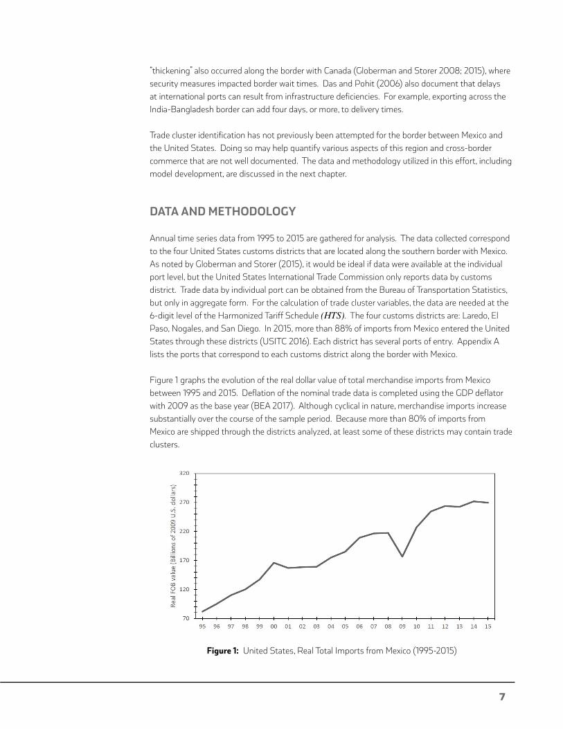
Figure 1 graphs the evolution of the real dollar value of total merchandise imports from Mexico between 1995 and 2015. Deflation of the nominal trade data is completed using the GDP deflator with 2009 as the base year (BEA 2017). Although cyclical in nature, merchandise imports increase substantially over the course of the sample period. Because more than 80% of imports from Mexico are shipped through the districts analyzed, at least some of these districts may contain trade clusters.

Figure 1: United States, Real Total Imports from Mexico (1995-2015)


(9)TCdt = δ1GL6dt + δ2HH6dt + + δnOtherdt + edt...

.. .. .. .. ..

TCdt - TCd = δ1(GL6dt - GL6d ) + δ2(HH6dt - HH6d ) + + δn(Otherdt - Otherd ) + edt - ed

_ _ _ _ _...

(8)TCd = δ0 + δ1GL6d + δ2HH6d + + δnOtherd + ad + edt...

(7)TCdt = δ0 + δ1GL6d + δ2HH6dt + + δnOtherdt + ad + edt

_ _ _ _ _

...

(6)TC = f(GL6, HH6, Other)

OPWEST = OilPrice * (1 - Pipeline) (5)

HHPORT = ∑n X 2 (4)

HH = X 2 + X 2 + X 2 + + X 2

i=1 n

(3)1 2 3 n...

GLid = [ [ ]] = 1 - (2)( )Exportsid Importsid+ | | | |Exportsid Importsid- Exportsid Importsid--

Exportsid Importsid+ Exportsid Importsid+__

(1)


.. .. .. .. ..


_ _ _ _ _...



_ _ _ _ _

...




HH = X 2 + X 2 + X 2 + + X 2

i=1 n

(3)1 2 3 n...

(2)

( )TCdt =

CIFdt

FOBdt

FOBdt- 100*_ (1)

This study attempts to analyze the extent to which transportation costs are influenced by trade clusters. Toward that end, it is necessary to determine whether a specific zone in the border region can be defined as a trade cluster. Also, a reliable measure for transportation costs is needed.

To quantify transportation costs, prior studies utilize the CIF / FOB ratio as a measure of transportation costs ((Limao and Venables 2001; Walke and Fullerton 2014; Globerman and Storer 2015). That ratio captures transportation costs using data on CIF (cost, insurance, and freight) and FOB (free on board) merchandise trade values. CIF represents the value of imports when they arrive at the importing country, which includes insurance and freight costs. FOB represents the value of imports reported by exporting countries. In other words, the FOB value is equal to the CIF value minus insurance and freight costs (De 2006). Both CIF and FOB values are reported by the United States International Trade Commission (USITC).

( CIF - FOB )_dt dtTCdt = * 100 (1)FOBdt

Equation 1 illustrates how the transportation cost ratio is calculated. TC is the transportation cost ratio, subscript d stands for each district, while subscript t stands for time. It is not necessary to deflate the transportation cost ratio because it is not expressed in monetary units (Walke and Fullerton 2014). It is important to mention that the CIF value includes insurance and freight costs from the starting point or foreign country all the way to the final destination. It does not directly control for changes in distance and no attempt is made to do so. Instead, as done in a similar study that analyzes transport costs and trade clusters at the northern border, average shipping distances are assumed not to change during the sample period (Globerman and Storer 2015). Advances in data assembly may one day allow that question to be directly examined (Jarmin 2019).

Figure 2 provides graphs of the calculated transportation cost ratios. As can be observed, overall transportation costs have decreased since 1995. After 2001, transportation costs temporarily increased across all districts. Two recent studies indicate that increases in border security measures after 11 September 2001 impacted the CIF/FOB ratio (Globerman and Storer 2008; Walke and Fullerton 2014). Qualitative variables equal to zero from 1995 to 2000 and equal to one from 2001 to 2015 can help control for this effect.

As noted above, a trade cluster is defined as a geographical concentration where similar industries, or closely related industries, trade merchandise. Grubel-Lloyd and Herfindahl-Hirschman indexes are selected to operationalize this concept. The Grubel-Lloyd (GL) index is a widely utilized method for determining the degree of intra-industry trade (Grubel and Lloyd 1975; OECD 2002; Fullerton, Sawyer, and Sprinkle 2011). Equation 2 shows how that index is calculated.

( Exports + Imports ) - Exports - Imports Exports - ImportsGL = [ id_id | id id | ] = 1 - [ | _id id | ] (2)id Exports + Imports Exports + Importsid id id id

9

Figure 2: Customs District 100*(CIF – FOB)/FOB Ratios, 1995-2015

Intra-Industry trade occurs when a country simultaneously imports and exports similar goods, often at consecutive stages of production. A GL index is calculated for each industry (i) within each district (d). Each index is weighted by the share of total trade of each industry over total trade within the district. The indices provide information on the extent to which similar or closely related goods are traded within the districts. If the GL index is equal to one, this indicates that a country imports and exports similar products. In Equation 2, when exports equal imports, then GL equals one. At the other extreme, if a country does not export any of the goods that it imports, or vice versa, then GL equals zero. Thus, the GL index can take on values between zero and one (Van Marrewijk 2008). If intra-industry trade is present in a customs district, variations in transportation costs may result from just-in-time inventory strategies that cause companies to spend more on transportation as a means for reducing inventory costs (Globerman and Storer 2015).

The Herfindahl-Hirschman index (HH) is utilized by the Department of Justice of the United States for market concentration measurement in anti-trust analyses. It is typically calculated by squaring the market percentage share of each firm and then adding the numbers. The HH index approaches zero when the market is well distributed and approaches 10,000 points as the market becomes more concentrated (USDJ 2015). In this study, the HH index is calculated using decimals instead of percentage points. That forces the HH index to range from zero, when industries are well distributed, to one, when industries are highly concentrated. The 0 to 1 range matches that employed for the GL index above. Equation 3 shows how the HH index is calculated.



.. .. .. .. ..


_ _ _ _ _...



_ _ _ _ _

...



HHPORT = ∑n X 2 (4)i=1 n

(3)



( )TCdt =

CIFdt

FOBdt

FOBdt- 100*_ (1)


.. .. .. .. ..


_ _ _ _ _...



_ _ _ _ _

...



(4)

HH = X 2 + X 2 + X 2 + + X 2 (3)1 2 3 n...



( )TCdt =

CIFdt

FOBdt

FOBdt- 100*_ (1)

...HH = X 12 + X 22 + X 32 + + X n2 (3)

In Equation 3, Xn is the share, expressed in decimals, of each industry in total exports or total imports. As in Globerman and Storer (2015), an HH index is calculated for imports, with another index calculated for exports, and both are then added together. The GL and HH indices are calculated utilizing industry-level data. Industries are identified using the Harmonized Tariff Schedule (HTS) at the 6-digit level of specificity. The data are obtained from the United States International Trade Commission (USITC 2016). If the exports and imports of a customs district are concentrated among a small group of key industries, and those industries are very similar, that district can be characterized as having a trade cluster. The degree of concentration and similarity may help explain variations in merchandise trade transportation costs (Globerman and Storer 2015).

HHPORT = ∑n X 2 (4)i=1 n

Equation 4 shows how the variable HHPORT is calculated. X is the share of total trade by ports and n is the number of ports. Since each custom district has several ports of entry, each port has a share of total trade in the customs district. The Bureau of Transportation Statistics (BTS 2017) publishes aggregate trade data for each port. Similar to HH6, the trade shares are expressed using decimals, resulting in an HHPORT index that ranges in value between zero and one. As total trade within a custom district becomes more concentrated in a single port, the value of HH6 approaches one. As total trade becomes more evenly distributed among the ports in a district, the value of HH6 will approach zero.

Table 1 lists all of the variables included in the data sample. Along with the name assigned to each variable, Table 1 also provides definitions, units of measure, and data sources. A total of eleven variables are collected for each of the four customs districts in the sample. The time period analyzed is 1995-2015.

In addition to the industry (GL6) and trade concentration (HH6) variables, several other variables are also included in the sample. LEXIM is the natural logarithm of exports plus imports. It is used to quantify the effects of economies of scale on transportation costs. It also is expected to be correlated with backhaul shipments, further exerting a negative impact on transportation costs (Globerman and Storer 2015). TRUCK and PIPELINE are variables that measure the percentages of imports that enter each customs district by those modes of transportation. Trade data are reported by ports of entry and by mode of transportation, making it relatively easy to calculate those variables (BTS 2017).

tomf

Sticky Note

Change to read: each customs district


.. .. .. .. ..


_ _ _ _ _...



_ _ _ _ _

...


(5)


HH = X 2 + X 2 + X 2 + + X 2

i=1 n

(3)1 2 3 n...



( )TCdt =

CIFdt

FOBdt

FOBdt- 100*_ (1)

11

Table 1: Variables Names and Definitions

Variable Name Definition Unit of Measure Data Source

TC (CIF – FOB) / FOB ratio transport cost measure. Percent USITC

GL6

HH6

LEXIM

Grubel-Lloyd intra-industry trade index using 6-digit Harmonized Tariff Schedule data for imports and exports.

Sum of the Herfindahl-Hirschman industry share of trade indices for exports and imports using 6-digit Harmonized Tariff Schedule data.

Natural logarithm of the sum of exports and imports through each customs district.

Percent

Percent

Natural Logarithm

USITC

USITC

USITC

HHPORT Herfindahl-Hirschman index for port concentration. Percent BTS

TRUCK Percent of total merchandise imports transported by cargo trucks. Percent BTS

PIPELINE Percent of total merchandise imports transported by pipeline. Percent BTS

OPWEST

TREND

D2001

D2001TREND

Interaction term for the product of the West Texas Intermediate oil price with the share of merchandise imports transported by truck or rail.

Simple time trend variable.

A binary variable for post-9/11 border inspection administrative changes.

An interaction term between the 9/11 dummy and time trend variables.

US$

1995 = 1 2015 = 21

1995 - 2000 = 0 2001 - 2015 = 1

Discrete Numbers

BTS St. Louis Fed

BRMP

BRMP

BRMP

OPWEST is an interaction variable between the West Texas Intermediate oil price and the non-pipeline (truck and rail) merchandise transportation mode shares. Equation 5 shows how the OPWEST interaction variable is calculated. The share of trade by truck and railroad is multiplied by the oil price. This interaction term is designed to help quantify oil price change impacts on transportation costs by those transportation modes in each of the four customs districts (Globerman and Storer 2015).


Table 2 reports summary statistics for all variables included in the sample. The TC transportation cost ratio has a mean of 0.86 across all four customs districts. Recalling how TC is calculated using Equation (1), that implies that insurance and freight charges equal approximately 0.86 percent of the total merchandise value in this sample. That is lower than what is documented for trade in general and probably reflects the close proximity of manufacturing facilities in northern Mexico to the border (Rodrigue 2017). The TC estimates are slightly asymmetric. More specifically, the observations for TC are right-skewed (positive). Compared to a Gaussian distribution, the TC data are also somewhat platykurtic.


.. .. .. .. ..


_ _ _ _ _...



_ _ _ _ _

...

(6)



HH = X 2 + X 2 + X 2 + + X 2

i=1 n

(3)1 2 3 n...



( )TCdt =

CIFdt

FOBdt

FOBdt- 100*_ (1)


.. .. .. .. ..


_ _ _ _ _...


(7)

_ _ _ _ _




HH = X 2 + X 2 + X 2 + + X 2

i=1 n

(3)1 2 3 n...



( )TCdt =

CIFdt

FOBdt

FOBdt- 100*_ (1)


.. .. .. .. ..


_ _ _ _ _...

(8)

(7)TCdt = δ0 + δ1GL6d + δ2HH6dt + + δnOtherdt + ad + edt...




HH = X 2 + X 2 + X 2 + + X 2

i=1 n

(3)1 2 3 n...



( )TCdt =

CIFdt

FOBdt

FOBdt- 100*_ (1)


_ _ _ _ _

Table 2: Summary Statistics

TC GL6 HH6 LEXIM HHPORT TRUCK PIPELINE OPWEST

Mean 0.861 0.254 0.064 10.683 0.666 0.856 0.000267 53.070

Median 0.835 0.240 0.057 10.023 0.617 0.866 1.20*10-6 48.642

Maximum 2.238 0.396 0.170 12.522 0.989 0.999 0.0024 99.670

Minimum 0.211 0.114 0.016 9.096 0.414 0.603 0.000 14.418

Std. Dev. 0.530 0.254 0.064 0.856 0.161 0.121 0.000581 30.240

Skewness 0.619 0.455 0.854 0.297 0.571 -0.219 2.333 0.281

Kurtosis 2.295 2.254 3.274 2.365 2.072 1.737 7.227 1.539

GL6 is right-skewed and slightly platykurtic. The observations for HH6 are also positively skewed, but slightly leptokurtic. The data for LEXIM are distributed in a fairly symmetric manner about the mean. The port concentration variable, HHPORT, has a mean of 0.66, reflecting fairly high degrees of trade flow concentrations among each of the customs districts. Observations PIPELINE are clustered near 0.0 because Mexico exports very little using this mode of transportation.

Equation 6 shows the implicit functional form that is utilized to model transportation costs.

TC = f(GL6, HH6, Other) (6)

In Equation 6, TC is transportation costs as approximated by the (CIF – FOB) / FOB ratio. GL6 is the Grubel-Lloyd index for industry similarity. HH6 is the sum of the Herfindahl-Hirschman index for import concentration and the Herfindahl-Hirschman index for export concentration. Other variables listed in Table 1 are also utilized to control for additional factors that influence transportation costs. A fixed effects procedure is utilized that controls for time constant unobserved effects by employing a transformation that removes them before estimation (Wooldridge 2006).

...TC = δ + δ GL6 + δ HH6 + + δ Other + a + e (7)dt 0 1 d 2 dt n dt d dt

Equation 7 shows the model without fixed effects. Subscripts d and t stand for district and time, respectively. The term ad represents the unobserved fixed effect for each district and edt is the error term. Averaging Equation 7 over time yields:

...TC = δ + δ GL6 + δ HH6 + + δ Other + a + e (8)d 0 1 d 2 d n d d dt

13


.. .. .. .. ..



_ _ _ _ _

...




HH = X 2 + X 2 + X 2 + + X 2

i=1 n

(3)1 2 3 n...



( )TCdt =

CIFdt

FOBdt

FOBdt- 100*_ (1)

(9)


_ _ _ _ _...



_ _ _ _ _

...




HH = X 2 + X 2 + X 2 + + X 2

i=1 n

(3)1 2 3 n...



( )TCdt =

CIFdt

FOBdt

FOBdt- 100*_ (1)

_ _ _ _ _

Equation 8 employs the sample average of each variable for each customs district. It is not necessary to write the over-bar on ad because it is constant over time. This also applies for the intercept term δ0. The fixed effect transformation requires subtracting Equation 8 from Equation 7.

...TC - TC = δ (GL6 - GL6 ) + δ (HH6 - HH6 ) + + δ (Other - Other ) + e - edt d 1 dt d 2 dt d n dt d dt d

.. .. .. .. .. ...TC = δ GL6 + δ HH6 + + δ Other + e (9)dt 1 dt 2 dt n dt dt

—̈Equation 9 is the simplified form of the fixed effects specification, where (TC)dt=TCdt - (TC)d and the same convention is used for the independent variables and the error term. This final equation is estimated using pooled ordinary least squares (OLS). The constant terms, ad and δ0, are eliminated by the subtraction of Equation 8 from Equation 7. Parameter estimation results and implications are summarized in the next section.


ESTIMATION RESULTS

Table 3 summarizes estimation output for the fixed effects regression for transportation costs. Fixed effects modeling facilitates controlling for unobserved variables that are constant over time (Wooldridge 2006). As noted above, there is no universally accepted way to control for shipping distances so it is assumed that merchandise transport distances for each customs districts do not change, on average, over time. Clearly, distances traveled are different among those customs districts (Globerman and Storer 2015). Walke and Fullerton (2014) mention that the type of commodities traversing the United States - Mexico border are relatively similar over time, so this should be captured by the fixed effect estimates. Also, each district may differ in other respects (Cortright 2006) and these differences can potentially influence values for the dependent variable. The cross-section fixed effects show how these unobserved time-invariant factors affect transportation costs for each district.

Table 3: Fixed Effects Output for the TC = (CIF – FOB) * 100 / FOB Ratio

Regression with Driscoll-Kraay standard errors Number of observations = 84

Method: Fixed-effects regression Number of groups = 4

Group variable (i): DISTRICT F(10, 3) = 73.48

Maximum lag = 2 Prob > F = 0.0023

Breusch-Pagan LM Chi-squared statistic = 10.66 within R-squared = 0.6304

TC Coefficient Drisc/Kraay Std. Err.

t P > | t | [95% Conf. Interval]

CONSTANT 2.450 1.468 1.702 0.187 -2.173 7.172

GL6 -1.153 0.437 -2.640 0.078 -2.542 0.237

HH6 -1.605 0.495 -3.242 0.048 -3.179 -0.031

LEXIM -0.193 0.124 -1.553 0.218 -0.588 0.202

HHPORT -0.372 0.110 -3.381 0.043 -0.722 -0.022

TRUCK 1.382 0.524 2.639 0.078 -0.284 3.049

PIPELINE -52.753 34.869 -1.512 0.228 -163.722 58.216

OPWEST 0.0001 0.0006 0.175 0.872 -0.0018 0.0020

TREND -0.040 0.017 -2.425 0.094 -0.093 0.0126

D2001 -0.271 0.0552 -4.910 0.016 -0.447 -0.095

D2001TREND 0.053 0.011 4.796 0.017 0.018 0.087

Results in Table 3 are estimated employing the Driscoll and Kraay (1998) technique for computing robust standard errors by taking into account heteroscedasticity, autocorrelation, and cross-sectional dependence for panel datasets. Vogelsang (2012) provides an analysis of the validity of the robust standard errors proposed by Driscoll and Kraay (1998) in the context of the fixed effects estimator. Hoechle (2007) states that Driscoll and Kraay (1998) robust standard errors are more appropriate

15

compared to other methods of robust standard error estimation when there is cross-sectional dependence. The Breusch and Pagan (1980) Lagrange multiplier (LM) test is used to examine the hypothesis that the residuals are independent across each cross-section. The Breusch and Pagan LM test works best when T > N (De Hoyos and Sarafidis, 2006). The null hypothesis of cross-sectional independence is rejected at the one percent significance. Consequently, the Hoechle (2007) procedure is employed for all of the parameter estimates reported in Table 3.

Of course, employment of customs district data imposes an assumption that port fixed effects are jointly equal to zero. Until trade data by individual port can be obtained at the 6-digit HTS level, there is no way of testing whether that assumption is reasonable. It does seem plausible from the perspective that much of the trade volumes through each district tend to be concentrated at individual ports. Given that, any potential misspecification bias, at least at present, is limited. Given the new advances in data proliferation, it may eventually become possible to one day test that proposition (Jarmin 2019).

When estimating an equation with fixed effects, the time-demeaned transformation eliminates unobserved fixed effects along with the constant term (Wooldridge 2006). Although the data are demeaned, the estimation output includes a constant term. The constant coefficient of 2.450 in Table 3 represents the average of the fixed effects, in other words, the average of the intercepts of the four customs districts.

Table 4: Cross-Section Fixed Effects and Customs District Intercept Coefficients

Customs District Cross-Section Fixed Effects District Intercept

San Diego -0.662 1.837

Nogales 0.661 3.161

El Paso -0.549 1.951

Laredo 0.550 3.050

Column 2 of Table 4 reports the cross-section fixed effects. These effects represent the deviations of each cross-section intercept from the constant coefficient in Table 3. These estimates indicate that San Diego and El Paso, the largest urban economies in the sample, observe the lowest transport costs. Given the size of these metropolitan economies, plus long business histories in merchandise trade, economies of agglomeration may be embodied by the estimates shown in Table 4 (Venables 2007).

Column 3 of Table 4 reports the calculated intercept term for each district. The district intercepts allow measuring the effect of the time-constant unobserved variables on the transportation cost ratios for each district, while controlling for the observed independent variables. For example, transportation costs for the El Paso district are estimated to equal 1.95 percent of the value of imports after accounting for the impacts of the other independent variables in Table 3. The Laredo and Nogales customs districts exhibit the highest transportation cost ratios, 3.05 and 3.16 percentage points, respectively.


The higher transportation cost ratios in those districts do not appear to be due to the types of merchandise that are imported through those ports. Table 5 reports the top three HTS chapters of imports for each district for six years from 1990 through 2015. All four customs districts process relatively high volumes of transportation equipment and electronic equipment. Although Nogales processes high volumes of fruit and vegetable imports, the goods mix imported through Laredo is very similar to that of El Paso. Finally, with a calculated intercept of 2.32 percentage points, the San Diego district has the lowest transportation cost ratio, probably reflecting shorter average distances for shipments originating from Tijuana and Mexicali.

The intercepts in Table 4 differ in magnitude from the northern border coefficients obtained by Globerman and Storer (2015). In this study, the average of district intercepts is 2.99 percentage points. The corresponding average for the border between the United States and Canada is 10.27 percentage points. Buffalo and St. Albans are the districts with the highest and lowest transportation costs due to fixed effects, with estimated intercepts of 10.99 and 9.40 percentage points, respectively. The time-invariant factors on the southern border of the United States have relatively lower impacts on transportation costs than is the case on the northern border. The mix of goods imported may influence the difference in transportation cost ratios for the two borders. Table 6 shows that Canada exports large volumes of energy products to the United States.

Table 5: Top 3 United States Imports from Mexico by Customs District

San Diego Nogales El Paso Laredo

HTS % HTS % HTS % HTS %

85 37% 87 28% 85 56% 85 25%

1990 84 10% 7 20% 98 7% 87 22%

90 6% 85 18% 84 6% 84 12%

85 39% 87 29% 85 53% 87 27%

1995 84 12% 85 22% 84 9% 85 21%

87 7% 7 12% 90 8% 84 12%

85 40% 85 34% 85 47% 87 32%

2000 84 16% 87 22% 84 13% 85 20%

87 6% 7 8% 90 7% 84 14%

85 44% 85 29% 85 40% 87 26%

2005 84 10% 87 14% 84 20% 85 20%

87 7% 7 12% 87 9% 84 16%

85 49% 87 35% 84 35% 87 27%

2010 90 9% 85 16% 85 31% 85 21%

87 8% 7 13% 87 11% 84 16%

85 43% 87 33% 84 36% 87 32%

2015 87 14% 85 18% 85 24% 85 18%

90 9% 7 10% 87 15% 84 16%

17

Harmonized Tariff Schedule Chapters:

7: Edible vegetables and certain roots and tubers

84: Machinery and mechanical appliances; nuclear reactors; boilers

85: Electrical machinery and equipment; television recorders/reproducers; sound recorders/reproducers

87: Vehicles, other than railway or tramway rolling stock, and parts and accessories thereof

90: Optical, photographic, cinematographic, measuring, checking, precision, medical/surgical apparatuses

98: Special classification provisions: not either specified or included

Source: Table from Walke and Fullerton (2014), data from USITC (2016)

The Grubel-Lloyd index (GL6) for intra-industry trade is calculated using the Harmonized Tariff Schedule (HTS) at the 6-digit level of classification for exports and imports. The parameter estimate is negative, indicating that transportation costs decline as the similarity of goods being traded increases (Table 3). The coefficient suggests that, when the GL6 index increases by one unit, transportation costs will decrease by 1.17 units of the (CIF – FOB) / FOB ratio. Greater intraindustry trade probably increases the likelihood of obtaining backhaul transport contracts. Industries engaged in intra-industry trade also tend to locate in cities closer to the border and, generally, ship freight over smaller distances. In the case of the Canada-United States border, the GL6 regression coefficient is positive. The latter finding is attributed to the prominence of just-in-time inventory management techniques that place a premium on timely delivery and may, consequently, reduce backhaul opportunities and/or volumes (Globerman and Storer 2015).


Table 6: Top 3 United States Imports from Mexico and Canada

Mexico Canada

HTS % HTS %

85 33.23% 87 33.54%

1990 87 14.68% 84 8.82%

84 9.43% 27 7.21%

85 31.40% 87 32.38%

1995 87 18.11% 84 8.60%

84 10.82% 27 6.60%

85 30.09% 87 28.94%

2000 87 21.87% 27 10.21%

84 13.43% 84 8.05%

85 28.75% 87 25.73%

2005 87 18.53% 27 17.30%

84 15.22% 84 7.42%

85 27.14% 87 21.96%

2010 87 21.16% 27 18.92%

84 18.22% 84 7.31%

87 26.21% 87 24.22%

2015 85 23.14% 27 12.48%

84 18.19% 84 7.85%

Harmonized Tariff Schedule Chapters:

27: Mineral fuels, mineral oils, and distillation products; bituminous substances; mineral waxes

84: Machinery and mechanical appliances; nuclear reactors; boilers

85: Electrical machinery/equipment; tv recorders/reproducers; sound recorders/reproducers

87: Vehicles, other than railway or tramway rolling stock, plus parts and accessories thereof

Source: Data from USITC (2016)

Herfindahl-Hirschman sub-indices are calculated for exports and imports using the Harmonized Tariff Schedule (HTS) at the 6-digit level of classification. HH6 is the sum of those two sub-indices. The HH6 coefficient in Table 3 suggests that a one unit increase in the concentration of imports or exports in particular goods diminishes costs related to movements of merchandise from one country to another by 1.17 percentage points of the (CIF – FOB / FOB) dependent variable ratio. These effects are likely attributable to the increasing probability of finding backhaul opportunities. Also potentially contributing to this is greater specialization among border personnel at individual customs district POE in handling shipment and customs requirements for those particular goods categories. The coefficient estimate does not quite satisfy the standard significance criterion, but the magnitude is economically significant. In contrast to the negative coefficient reported in Table

19

---

--- ---

Dis

tric

t

3, Globerman and Storer (2015) find that HH6 positively impacts transportation costs across the northern border. That study indicates that this may be due to extremely high degrees of specialization in certain industries that effectively preclude finding backhaul shipments.

The parameter estimate for the total trade variable (LEXIM, the logarithm of the sum of exports and imports) is negative and significant in Table 3. This coefficient indicates that a one percent increase in total trade results in a reduction of 0.23 percentage points in the transportation cost ratio for merchandise arriving at the international boundary between the two countries. This negative relationship can be attributed to higher probabilities of finding backhaul shipments due to greater volumes of bilateral trade within a customs district (Globerman and Storer 2015). The total trade variable also helps to identify the effect of economies of scale on transportation costs. One reason that countries trade, of course, is to take advantage of economies of scale (Krugman, Obstfeld, and Melitz 2012). The same effect is reported for the northern border with Canada, where increases in the total trade variable also reduce transportation costs, but to a greater extent than indicated by Table 3.

The HHPort variable is designed to measure the concentration of merchandise trade flows among ports of entry in a customs district. Higher values of this index mean that more of the trade is concentrated among a few ports. Lower values mean that trade is more evenly distributed among the various ports. The coefficient for this variable in Table 3 is negative and statistically significant. It indicates that, as the Herfindahl-Hirschman port concentration index increases by one unit, the transportation cost (CIF – FOB) / FOB ratio decreases by -0.4985 percentage. Similar to what Globerman and Storer (2015) report for the northern border with Canada, the magnitude of the HHPort parameter is economically significant as well as negative.

Table 7 reports the percentage of district-wide trade flows that go through each port. The ports of Otay Mesa, Nogales, El Paso, and Laredo handle the highest individual percentages of total trade in each respective district (BTS 2017). Because those ports are more intensively utilized, customs officers stationed there tend to be more knowledgeable about import procedures and the kinds of products that are imported through these locations. That helps make delays less common and probably reduces transportation costs. Furthermore, the likelihood of landing backhaul contracts may also be higher when trade volumes are concentrated in a few heavily transited ports (Globerman and Storer 2015).

Table 7: Average Percentage of Total District Trade through each Port (1995-2015)

Ports

San Diego San Ysidro Otay Mesa Tecate Calexico Others % 2.82 67.59 2.37 25.81 1.41

Nogales San Luis Nogales Douglas Others % 5.75 86.70 6.82 0.73

El Paso Santa Teresa El Paso Others % 12.98 86.27 0.75

Laredo Eagle Pass Laredo Hidalgo Brownsville Others % 8.35 69.96 11.72 7.54 2.43

Source: Bureau of Transportation Statistics (BTS 2017)


TRUCK, PIPELINE, and OPWEST are utilized to control for other factors that might affect transportation costs. TRUCK is a measure of the percentage of merchandise imports that travel by truck. The coefficient estimate for this regressor in Table 3 indicates that, when the share of trade shipped by truck rises by one percentage point, the (CIF – FOB) / FOB ratio is expected to increase by 1.19 percentage points. This result confirms the effect hypothesized for the northern border in Globerman and Storer (2015), but the computed t-statistic does not surpass the 5-percent significance threshold.

PIPELINE measures the share of merchandise imports that traverse the border via pipeline. The estimated coefficient in Table 3 is negative, implying that trade related transportation costs decline as pipeline shipments increase. More precisely, the estimated coefficient suggests that, when this variable increases by one percentage point, the transportation cost (CIF – FOB) / FOB ratio decreases by slightly more than 12 percentage points. The coefficient magnitude for this variable may be unrealistically large. It also fails to satisfy the standard significance criterion. Data from the Bureau of Transportation Statistics indicate that imports into the United States by pipeline are almost null at southern border (BTS 2017). For example, the percentage of imports by pipeline through the El Paso district is zero for each year in the sample. Given the limited volume of imports by pipeline at the southern border, the size of the pipeline coefficient should be interpreted with caution. It does suggest, however, that the recent investments to increase energy pipeline export capacity from the United States to northern Mexico will reduce overall trade related transport costs (Proctor 2019; ICVS 2019).

That is very different from what has been reported for the United States border with Canada. Across that boundary, a negative and significant relationship is estimated for between pipeline imports and transportation costs (Globerman and Storer 2015). Of course, pipeline imports from Canada are more prevalent than pipeline imports from Mexico. In Table 6, mineral fuel and mineral oils are consistently among the top three categories of merchandise imports from Canada throughout the entire sample period.

OPWEST is an interaction term calculated by the product of the West Texas Intermediate oil price and the share of imports transported using modes of transportation other than pipelines. This interaction term helps to measure the impact on transportation costs by trucks and rail when there are changes in oil prices. As expected, the regression parameter indicates that a positive relationship exists between the oil price variable and the dependent variable (Table 3). This coefficient has a magnitude of 0.0011. In economic terms, the total dollar equivalent of a one unit increase in OPWEST is a transportation cost increase, by truck and rail, of only $401,582 USD across all four customs districts. Not surprisingly, the coefficient is not statistically distinguishable from zero. In all likelihood, the fixed costs of cargo trucks and rail dominate those of the marginal fuel costs, represented in this sample by the West Texas Intermediate oil price. In contrast, for the Canada-United States border, the same interaction variable exerts a stronger effect on the transportation cost ratio (Globerman and Storer 2015).

Both Globerman and Storer (2008) and Walke and Fullerton (2014) provide evidence that transportation costs increased significantly after the terrorist attacks in 2001 at the southern and northern borders of the United States, respectively. In order to assess potential impacts of this event, a dummy variable, a trend variable, and an interaction term are employed. Table 3 reports the

21

estimated output allowing for 9/11 effects. In most cases, the explanatory variables have the same signs and magnitudes as in Table 3 and the interpretations are the same.

In Table 3, the TREND coefficient is negative as hypothesized. This inverse relationship is broadly discernible in the (CIF – FOB) / FOB ratio graphs for each customs district in Figure 2. The dummy variable (D2001) also has a negative parameter estimate that is statistically significant at the 5-percent level. This coefficient captures the difference between intercepts in the periods before and after 2001. Because transportation costs declined prior to 2001, the intercept for the 20012015 period is lower (Walke and Fullerton 2014).

In accordance with Globerman and Storer (2008) for the northern border with Canada, as well as Walke and Fullerton (2014) for the southern border with Mexico, an interaction term between the dummy and the trend variables (D2001TREND) is also employed. The parameter estimate for this interaction variable is consistent with what is documented in the earlier studies, as it is both positive and statistically significant. The visible increases in the (CIF – FOB / FOB) ratio subsequent to the imposition of the post-9/11 security measures in each customs district are, thus, corroborated by the results reported in Table 3.

CONCLUSION

This study analyzes the extent to which transportation costs are influenced by trade clusters at different locations along the border between the United States and Mexico. Sample data are collected for a two-decade period from 1995 through 2015. From west to east, the southern United States border region has four customs districts: San Diego, Nogales, El Paso, and Laredo. Transportation cost ratios are calculated for each district as TC = (CIF – FOB) / FOB. Grubel-Lloyd indices for intra-industry trade similarity and Herfindahl-Hirschman indices for industry concentration are calculated and employed as variables that identify trade clusters.

Parameter estimation of the two equations employs a fixed effect procedure that calculates robust standard errors by allowing for heteroscedasticity, autocorrelation, and cross-sectional dependence. The first equation includes the trade cluster variables and a set of control variables. The second model also controls for potential 9/11 effects on transportation costs. Empirical results indicate that the districts of Laredo and Nogales exhibit the highest transportation cost ratios among the four districts due to time-invariant factors. While the types of merchandise imported through each district are similar, other fixed factors such as distance that affect the documented transport costs.

Statistically significant impacts between trade cluster variables and transportation costs are confirmed by the regression analysis. Higher levels of intra-industry trade are associated with lower transportation costs, albeit with some degree of uncertainty. Higher levels of trade concentration are also found to reduce transportation costs in statistically reliable manners. The magnitudes of the GL6 and HH6 coefficients are also economically significant. Controlling for the effects of 9/11 terrorist attacks on administrative and inspection practices at the ports of entry also improves empirical outcomes.

The fixed effect results indicate that the time-invariant components of transportation costs are


higher at northern border ports than at the southern ports of entry examined in this study. The impacts of trade similarity and industry concentration on southern border transportation costs are also found to be opposite of the effects documented for the border with Canada. For the border with Mexico, negative coefficients are tallied for both GL6 and HH6, perhaps as a consequence of greater backhaul opportunities. A helpful step in clarifying the latter discrepancy might be provided by the acquisition of shipping distance data to augment the inclusion of transportation cost ratios and trade clusters indices for the various ports and port districts along both borders.

Implementation of the North American Free Trade Agreement led to numerous infrastructure investments that helped lower merchandise trade transport costs. That possibility also exists should the United States – Mexico – Canada Agreement be implemented in 2020 (or later). While the new trilateral agreement does contain administrative constraints that may cause inspection delays and disputes, new technologies and streamlined inspection procedures designed to expedite trade will also be introduced. The net impacts of these developments cannot, yet, be assessed, but should be examined at some future point once data become available.

23

REFERENCES

Anderson, B. 2012. The Border and the Ontario Economy. Windsor, ON: University of Windsor Cross-Border Transportation Centre.

Anderson, J.E., and E. van Wincoop. 2004. “Trade Costs.” Journal of Economic Literature 42 (3): 691-751.

Baptista, R., and P. Swann. 1998. “Do Firms in Cluster Innovate More?” Research Policy 27 (5): 691-751.

Behar, A., and A.J. Venables. 2011. “Transport Costs and International Trade.” Chapter 5 in A Handbook of Transport Economics. Cheltenham, UK: Edward Elgar Publishing.

Breusch, T., and A.R. Pagan. 1980. “The Lagrange Multiplier Test and its Application to Model Specification in Econometrics.” Review of Economic Studies 47 (1): 239-253.

BEA. 2017. Implicit Price Deflators for Gross Domestic Product. Washington, DC: United States Bureau of Economic Analysis.

BTS. 2017. North American Transborder Freight Data. Washington, DC: United States Bureau of Transportation Statistics.

Cortright, J. 2006. Making Sense of Clusters: Regional Competitiveness and Economic Development. Washington, DC: Brookings Institution.

Das, S., and S. Pohit. 2006. “Qualifying Transport, Regulatory and other Costs of Indian Overland Exports to Bangladesh.” World Economy 29 (9): 1227-1242.

De, P. 2006. Why Trade Costs Matter? Bangkok, TH: UNESCAP.

De Hoyos, R.E., and V. Sarafidis. 2006. “Testing for Cross-Sectional Dependence in Panel-Data Models.” Stata Journal 6 (4): 482-496.

Delgado, M., M.E. Porter, and S. Stern. 2010. “Clusters and Entrepreneurship,” Journal of Economic Geography 10 (4): 495518.

Delgado, M., M.E. Porter, and S. Stern. 2014. “Clusters, Convergence and Economic Performance.” Research Policy 43 (10): 1785-1799.

Delgado, M., M.E. Porter, and S. Stern. 2016. “Defining Clusters of Related Industries,” Journal of Economic Geography 16 (1): 1-38.

Driscoll, J.C., and A.C. Kraay. 1998. “Consistent Covariance Matrix Estimation with Spatially Dependent Panel Data,” Review of Economics and Statistics 80: 549-560.

Fullerton, T.M., Jr. 2007. “Empirical Evidence Regarding 9/11 Impacts on The Borderplex Economy.” Regional & Sectoral Economic Studies 7 (2): 51-64.


REFERENCES (CONT.)

Fullerton, T.M., Jr., W.C. Sawyer, and R.L. Sprinkle. 2011. “Intra-Industry Trade in Latin America and the Caribbean.” International Trade Journal 25 (1): 74-111.

Globerman, S., and P. Storer. 2008. The Impacts of 9/11 on Canada-U.S. Trade. Toronto, ON: University of Toronto Press.

Globerman, S., and P. Storer. 2015. “Transportation Costs and Trade Clusters: Some Empirical Evidence from U.S. Custom Districts.” Research in Transportation Business & Management 16: 67-73.

Grubel, H.G., and P.J. Lloyd. 1975. Intra-Industry Trade: The Theory and Measurement of International Trade in Differentiated Products. London, UK: Macmillan.

Hanson, G.H. 2001. “U.S.-Mexico Integration and Regional Economies: Evidence from Border-City Pairs.” Journal of Urban Economics 50 (2): 259-287.

Hays, F.H., and S.G. Ward. 2011. “Understanding Market Concentration: Internet-Based Applications from the Banking Industry,” Journal of Instructional Pedagogies 5: 101-115.

Hoechle, D. 2007. “Robust Standard Errors for Panel Regressions with Cross-Sectional Dependence.” Stata Journal 7 (3): 281-312.

ICVS. 2019. “NuStar using new Pipelines to move Fuel into Northern Mexico.” Bulk Transporter (9 September).

Jarmin, R.S. 2019. “Evolving measurement for an Evolving Economy.” Journal of Economic Perspectives 33 (1): 165-183.

Jones, L.L., T. Ozuna, Jr., and M. Wright. 1991. The U.S.-Mexico Free Trade Agreement: Economic Impacts on the Border Region. College Station, TX: Texas Agricultural Market Research Center.

Krueger, A.O. 2000. “NAFTA’s Effects: A Preliminary Assessment.” World Economy 23 (6): 761-775.

Krugman, P.R., M. Obstfeld, and M.J. Melitz. 2012. International Economics: Theory & Policy, Boston, MA: Pearson.

Limao, N., and A.J. Venables. 2001. “Infrastructure Geographical Disadvantage, Transport Costs, and Trade.” World Bank Economic Review 15 (3): 451-479.

OECD. 2002. “Intra-Industry and Intra-Firm Trade and the Internationalization of Production.” OECD Economic Outlook 1 (12): 309-320.

Peach, J.T., and R.V. Adkisson. 2000. “NAFTA and Economic Activity along the U.S.-Mexico Border.” Journal of Economic Issues 34 (2): 481-489.

Porter, M.E. 2003. “The Economic Performance of Regions.” Regional Studies 37 (6&7): 549-578.

Proctor, D. 2019. “Pipeline Deal means more U.S. Natural Gas for Mexico Power Plants.” Power (28 August).

25

Rodrigue, J. 2017. The Geography of Transport Systems. New York, NY: Routledge.

USDJ. 2015. Herfindahl-Hirschman Index. Washington, DC: United States Department of Justice.

USITC. 2016. Interactive Tariff and Trade Dataweb, Washington, DC: United States International Trade Commission.

Van Marrewijk, C. 2008. “Intra-Industry Trade,” in Princeton Encyclopedia of the World Economy. Princeton, NJ: Princeton University Press.

Venables, A.J. 2007. “Evaluating Urban Transport Improvements.” Journal of Transport Economics and Policy 41 (2): 173-188.

Vogelsang, T.J. 2012. “Heteroskedasticity, Autocorrelation, and Spatial Correlation Robust Inference in Linear Panel Models with Fixed-Effects.” Journal of Econometrics 166 (2): 303-319.

Walke, A.G., and T.M. Fullerton, Jr. 2014. “Freight Transportation Costs and the Thickening of the U.S.–Mexico Border.” Applied Economics 46 (11): 1248-1258.

Wooldridge, J.M. 2006. Introductory Econometrics a Modern Approach. Cincinnati, OH: Thomson South-Western.


Appendix A: Southern Border Customs Districts and Ports

District Port

Laredo Brownsville, TX

Valley International Airport, Harlingen, TX

Edinburg User Fee Airport, TX

Progreso, TX

Hidalgo/Pharr, TX

Rio Grande City, TX

Roma, TX

Laredo, TX

Eagle Pass, TX

Del Rio, TX

El Paso Presidio, TX

Fabens, TX

El Paso International Airport, TX

El Paso, TX

Santa Teresa Airport, NM

Santa Teresa, NM

Columbus, NM

Albuquerque, NM

Nogales Douglas, AZ

Naco, AZ

Nogales, AZ

Tucson, AZ

Saasabe, AZ

Lukeville, AZ

San Luis, AZ

Phoenix, AZ

San Diego Andrade, CA

Calexico East, CA

Calexico, CA

Tecate, CA

Otay Mesa Station, CA

San Ysidro, CA

San Diego, CA

27

Appendix B: Historical Data

DIST YEAR TC TRUCK PIPELINE LEXIM GL6

El Paso 1995 0.4668 0.9805 0.0000 9.90 0.2623

El Paso 1996 0.5843 0.9806 0.0000 10.02 0.2691

El Paso 1997 0.5572 0.9837 0.0029 10.11 0.2687

El Paso 1998 0.4899 0.9797 0.0027 10.28 0.2324

El Paso 1999 0.4068 0.9860 0.0045 10.41 0.2179

El Paso 2000 0.2971 0.9578 0.0055 10.62 0.2192

El Paso 2001 0.2915 0.9551 0.0028 10.57 0.2245

El Paso 2002 0.2901 0.9437 0.0028 10.59 0.2308

El Paso 2003 0.2914 0.9359 0.0023 10.61 0.2192

El Paso 2004 0.3331 0.9328 0.0006 10.70 0.2132

El Paso 2005 0.3700 0.9233 0.0090 10.71 0.2500

El Paso 2006 0.3768 0.9075 0.0117 10.79 0.2720

El Paso 2007 0.3198 0.8920 0.0071 10.84 0.2549

El Paso 2008 0.3136 0.8840 0.0102 10.82 0.2637

El Paso 2009 0.3402 0.9046 0.0025 10.76 0.2334

El Paso 2010 0.2982 0.9012 0.0134 11.15 0.2163

El Paso 2011 0.2496 0.8945 0.0231 11.27 0.2138

El Paso 2012 0.2110 0.8872 0.0161 11.36 0.2303

El Paso 2013 0.2786 0.8919 0.0113 11.36 0.2292

El Paso 2014 0.2690 0.8803 0.0142 11.37 0.2250

El Paso 2015 0.2706 0.8883 0.0083 11.43 0.2288

Laredo 1995 1.4259 0.7760 0.0001 10.79 0.2811

Laredo 1996 1.3823 0.7562 0.0001 11.02 0.2926

Laredo 1997 1.1056 0.7931 0.0000 11.25 0.3354

Laredo 1998 1.0857 0.8154 0.0001 11.33 0.3582

Laredo 1999 0.9643 0.8101 0.0000 11.46 0.3428

Laredo 2000 0.9393 0.7678 0.0012 11.69 0.3776

Laredo 2001 0.8813 0.7487 0.0022 11.63 0.3897

Laredo 2002 0.8875 0.7569 0.0055 11.62 0.3765

Laredo 2003 0.9085 0.7594 0.0008 11.63 0.3613

Laredo 2004 0.9493 0.7697 0.0007 11.75 0.3701

Laredo 2005 1.1137 0.7684 0.0017 11.81 0.3703

Laredo 2006 1.1169 0.7800 0.0020 11.93 0.3531

Laredo 2007 0.9305 0.7737 0.0050 11.99 0.3516


Appendix B: Historical Data (cont.)


Laredo 2008 0.9082 0.7821 0.0072 12.03 0.3730

Laredo 2009 1.0328 0.8171 0.0051 11.85 0.3647

Laredo 2010 1.0686 0.7946 0.0085 12.08 0.3808

Laredo 2011 0.9635 0.7868 0.0108 12.24 0.3857

Laredo 2012 0.9604 0.7802 0.0111 12.34 0.3945

Laredo 2013 1.0259 0.7832 0.0139 12.40 0.3962

Laredo 2014 0.9750 0.7859 0.0160 12.50 0.3929

Laredo 2015 0.9758 0.7900 0.0121 12.52 0.3933

Nogales 1995 1.8852 0.8073 0.0000 9.10 0.1139

Nogales 1996 2.0454 0.8427 0.0000 9.10 0.1581

Nogales 1997 1.7458 0.8223 0.0000 9.29 0.1656

Nogales 1998 1.6697 0.8106 0.0000 9.44 0.1618

Nogales 1999 1.6143 0.8476 0.0004 9.47 0.1605

Nogales 2000 1.2482 0.8397 0.0000 9.70 0.1885

Nogales 2001 1.4549 0.8243 0.0006 9.59 0.1800

Nogales 2002 1.6668 0.8355 0.0002 9.43 0.1718

Nogales 2003 1.9149 0.8797 0.0000 9.40 0.1737

Nogales 2004 2.2377 0.8888 0.0000 9.55 0.1823

Nogales 2005 1.8584 0.8694 0.0000 9.71 0.1787

Nogales 2006 1.4458 0.7307 0.0000 9.97 0.1460

Nogales 2007 1.5982 0.7659 0.0000 9.96 0.1570

Nogales 2008 1.5472 0.7226 0.0001 9.98 0.1497

Nogales 2009 1.5021 0.7219 0.0001 9.83 0.1573

Nogales 2010 1.4520 0.6930 0.0059 10.03 0.1737

Nogales 2011 1.2395 0.6874 0.0072 10.15 0.1699

Nogales 2012 1.3717 0.7351 0.0080 10.22 0.1781

Nogales 2013 1.2627 0.6383 0.0069 10.37 0.1436

Nogales 2014 1.5137 0.6609 0.0077 10.33 0.1541

Nogales 2015 1.3098 0.6614 0.0055 10.36 0.1608

San Diego 1995 0.5737 0.9925 0.0002 9.52 .2383

San Diego 1996 0.5323 0.9926 0.0001 9.73 0.2382

San Diego 1997 0.6248 0.9894 0.0001 9.89 0.2600

San Diego 1998 0.7877 0.9953 0.0001 10.01 0.2513

San Diego 1999 0.7660 0.9944 0.0001 10.12 0.2698

29


San Diego 2000 0.4502 0.9946 0.0001 10.26 0.2700

San Diego 2001 0.4837 0.9923 0.0001 10.24 0.2663

San Diego 2002 0.4662 0.9935 0.0000 10.31 0.2605

San Diego 2003 0.4460 0.9946 0.0000 10.30 0.2672

San Diego 2004 0.4261 0.9909 0.0000 10.41 0.2558

San Diego 2005 0.3999 0.9911 0.0000 10.51 0.2552

San Diego 2006 0.5586 0.9916 0.0000 10.65 0.2376

San Diego 2007 0.4596 0.9882 0.0000 10.70 0.2199

San Diego 2008 0.3252 0.9869 0.0011 10.70 0.2229

San Diego 2009 0.3171 0.9853 0.0068 10.55 0.2243

San Diego 2010 0.3027 0.9870 0.0030 10.66 0.2385

San Diego 2011 0.3040 0.9826 0.0052 10.74 0.2416

San Diego 2012 0.3452 0.9830 0.0040 10.79 0.2496

San Diego 2013 0.3772 0.9866 0.0048 10.83 0.2600

San Diego 2014 0.4270 0.9864 0.0058 10.92 0.2697

San Diego 2015 0.4445 0.9926 0.0024 11.01 0.2605

DIST YEAR HH6 HHPORT OPWEST TREND D2001

El Paso 1995 0.0557 0.9855 18.43 1 0

El Paso 1996 0.0568 0.9888 22.12 2 0

El Paso 1997 0.0535 0.9439 20.55 3 0

El Paso 1998 0.0568 0.9494 14.38 4 0

El Paso 1999 0.0454 0.9402 19.25 5 0

El Paso 2000 0.0440 0.9379 30.21 6 0

El Paso 2001 0.0435 0.9490 25.91 7 1

El Paso 2002 0.0480 0.9467 26.11 8 1

El Paso 2003 0.0703 0.9323 31.01 9 1

El Paso 2004 0.0646 0.9267 41.49 10 1

El Paso 2005 0.0523 0.9291 56.13 11 1

El Paso 2006 0.0511 0.9326 65.27 12 1

El Paso 2007 0.0405 0.9274 71.83 13 1

El Paso 2008 0.0488 0.9273 98.66 14 1

El Paso 2009 0.0717 0.8152 61.79 15 1

El Paso 2010 0.0835 0.6800 78.41 16 1


Appendix B: Historical Data (cont.)


El Paso 2011 0.1061 0.6375 92.69 17 1

El Paso 2012 0.1072 0.6319 92.54 18 1

El Paso 2013 0.1145 0.6432 96.87 19 1

El Paso 2014 0.1140 0.6427 91.85 20 1

El Paso 2015 0.1297 0.6235 48.26 21 1

Laredo 1995 0.0285 0.4141 18.43 1 0

Laredo 1996 0.0344 0.4417 22.12 2 0

Laredo 1997 0.0274 0.4647 20.61 3 0

Laredo 1998 0.0225 0.4768 14.42 4 0

Laredo 1999 0.0239 0.4935 19.34 5 0

Laredo 2000 0.0296 0.5245 30.34 6 0

Laredo 2001 0.0295 0.5261 25.92 7 1

Laredo 2002 0.0262 0.5308 26.04 8 1

Laredo 2003 0.0229 0.5212 31.05 9 1

Laredo 2004 0.0203 0.5300 41.48 10 1

Laredo 2005 0.0177 0.5143 56.54 11 1

Laredo 2006 0.0170 0.5010 65.92 12 1

Laredo 2007 0.0164 0.4977 71.98 13 1

Laredo 2008 0.0163 0.5086 98.95 14 1

Laredo 2009 0.0181 0.4981 61.63 15 1

Laredo 2010 0.0178 0.5017 78.80 16 1

Laredo 2011 0.0177 0.5184 93.86 17 1

Laredo 2012 0.0181 0.5328 93.01 18 1

Laredo 2013 0.0184 0.5399 96.62 19 1

Laredo 2014 0.0190 0.5382 91.68 20 1

Laredo 2015 0.0199 0.5488 48.07 21 1

Nogales 1995 0.0981 0.6859 18.43 1 0

Nogales 1996 0.0688 0.6904 22.12 2 0

Nogales 1997 0.0723 0.6970 20.61 3 0

Nogales 1998 0.0665 0.6962 14.42 4 0

Nogales 1999 0.0574 0.6874 19.33 5 0

Nogales 2000 0.0674 0.7281 30.38 6 0

Nogales 2001 0.0600 0.7500 25.97 7 1

Nogales 2002 0.0496 0.7663 26.18 8 1

31


Nogales 2003 0.0369 0.7634 31.08 9 1

Nogales 2004 0.0340 0.7615 41.51 10 1

Nogales 2005 0.0448 0.7532 56.64 11 1

Nogales 2006 0.1096 0.7987 66.05 12 1

Nogales 2007 0.0731 0.7747 72.34 13 1

Nogales 2008 0.0965 0.7959 99.66 14 1

Nogales 2009 0.0855 0.7886 61.95 15 1

Nogales 2010 0.1057 0.7919 79.01 16 1

Nogales 2011 0.0935 0.7640 94.20 17 1

Nogales 2012 0.0769 0.7547 93.29 18 1

Nogales 2013 0.1365 0.7680 97.30 19 1

Nogales 2014 0.1021 0.7629 92.45 20 1

Nogales 2015 0.1161 0.7713 48.39 21 1

San Diego 1995 0.0427 0.5524 18.43 1 0

San Diego 1996 0.0432 0.5373 22.12 2 0

San Diego 1997 0.0416 0.4520 20.61 3 0

San Diego 1998 0.0438 0.5349 14.42 4 0

San Diego 1999 0.0447 0.5107 19.34 5 0

San Diego 2000 0.0528 0.5355 30.38 6 0

San Diego 2001 0.0609 0.5622 25.98 7 1

San Diego 2002 0.0644 0.5468 26.18 8 1

San Diego 2003 0.0609 0.5344 31.08 9 1

San Diego 2004 0.0685 0.5363 41.51 10 1

San Diego 2005 0.0758 0.5374 56.64 11 1

San Diego 2006 0.1218 0.5530 66.05 12 1

San Diego 2007 0.1704 0.5618 72.34 13 1

San Diego 2008 0.1700 0.5778 99.56 14 1

San Diego 2009 0.1637 0.6111 61.53 15 1

San Diego 2010 0.1247 0.5894 79.24 16 1

San Diego 2011 0.1057 0.5836 94.38 17 1

San Diego 2012 0.0909 0.5795 93.68 18 1

San Diego 2013 0.0857 0.5822 97.51 19 1

San Diego 2014 0.0742 0.5836 92.63 20 1

San Diego 2015 0.0732 0.5781 48.54 21 1


________________________________________________________________________________

________________________________________________________________________________

________________________________________________________________________________

________________________________________________________________________________

________________________________________________________________________________

________________________________________________________________________________

The University of Texas at El Paso Announces

Borderplex Historical Data to 2018 UTEP is pleased to announce the 2020 edition of its primary source of Borderplex long-term historical economic information. Topics covered include demography, employment, personal income, retail sales, residential real estate, transportation, international commerce, and municipal water consumption. These data comprise the backbone of the UTEP Border Region Econometric Model developed under the auspices of a corporate research gift from El Paso Electric Company and maintained using externally funded research support from El Paso Water and Hunt Communities.

The authors of this publication are UTEP Professor & Trade in the Americas Chair Tom Fullerton and UTEP Border Region Modeling Project Associate Director & Economist Steven Fullerton. Dr. Fullerton holds degrees from UTEP, Iowa State University, Wharton School of Finance at the University of Pennsylvania, and University of Florida. Prior experience includes positions as Economist in the Executive Office of the Governor of Idaho, International Economist in the Latin America Service of Wharton Econometrics, and Senior Economist at the Bureau of Economic and Business Research at the University of Florida. Steven Fullerton has published research on Major League Baseball, the National Football League, and housing price fluctuations in Las Cruces.

The border long-range historical data reference can be purchased for $20 per copy. Please indicate to what address the report(s) should be mailed (also include telephone, fax, and email address):

Send checks made out to University of Texas at El Paso for $20 to:

Border Region Modeling Project - CBA 236 UTEP Department of Economics & Finance 500 West University Avenue El Paso, TX 79968-0543

Online orders can be placed via: https://secure.touchnet.net/C21711_ustores/web/product_detail.jsp?PRODUCTID=800

Request information from 915-747-7775 or [email protected] if payment in pesos is preferred.


https://secure.touchnet.net/C21711_ustores/web/product_detail.jsp?PRODUCTID=800

33

________________________________________________________________________________

________________________________________________________________________________

________________________________________________________________________________

________________________________________________________________________________

________________________________________________________________________________

________________________________________________________________________________

The University of Texas at El Paso Announces

Borderplex Long-Term Economic Trends to 2049 UTEP is pleased to announce the 2020 edition of its primary source of long-term structural trend border economic information. Topics covered include demography, employment, personal income, retail sales, residential real estate, transportation, international commerce, and municipal water consumption. Forecasts are generated utilizing the 250-equation UTEP Border Region Econometric Model developed under the auspices of a corporate research gift from El Paso Electric Company and maintained using externally funded research support from El Paso Water and Hunt Communities.

The authors of this publication are UTEP Professor & Trade in the Americas Chair Tom Fullerton and UTEP Border Region Modeling Project Associate Director & Economist Steven Fullerton. Dr. Fullerton holds degrees from UTEP, Iowa State University, Wharton School of Finance at the University of Pennsylvania, and University of Florida. Prior experience includes positions as Economist in the Executive Office of the Governor of Idaho, International Economist in the Latin America Service of Wharton Econometrics, and Senior Economist at the Bureau of Economic and Business Research at the University of Florida. Steven Fullerton has published research on Major League Baseball, the National Football League, and housing price fluctuations in Las Cruces.

The border long-range outlook through 2049 can be purchased for $25 per copy. Please indicate to what address the report(s) should be mailed (also include telephone, fax, and email address):

Send checks made out to University of Texas at El Paso for $25 to:

Border Region Modeling Project - CBA 236 UTEP Department of Economics & Finance 500 West University Avenue El Paso, TX 79968-0543

Online orders can be placed via: https://secure.touchnet.net/C21711_ustores/web/product_detail.jsp?PRODUCTID=810

Request information from 915-747-7775 or [email protected] if payment in pesos is preferred.


https://secure.touchnet.net/C21711_ustores/web/product_detail.jsp?PRODUCTID=810


The UTEP Border Region Modeling Project & UACJ Press Announce the Availability of

Basic Border Econometrics The University of Texas at El Paso Border Region Modeling Project is pleased to announce Basic Border Econometrics, a publication from Universidad Autónoma de Ciudad Juárez. Editors of this new collection are Martha Patricia Barraza de Anda of the Department of Economics at Universidad Autónoma de Ciudad Juárez and Tom Fullerton of the Department of Economics & Finance at the University of Texas at El Paso.

Professor Barraza is an award winning economist who has taught at several universities in Mexico and has published in academic research journals in Mexico, Europe, and the United States. Dr. Barraza currently serves as Research Provost at UACJ. Professor Fullerton has authored econometric studies published in academic research journals of North America, Europe, South America, Asia, Africa, and Australia. Dr. Fullerton has delivered economics lectures in Canada, Colombia, Ecuador, Finland, Germany, Japan, Korea, Mexico, the United Kingdom, the United States, and Venezuela.

Border economics is a field in which many contradictory claims are often voiced, but careful empirical documentation is rarely attempted. Basic Border Econometrics is a unique collection of ten separate studies that empirically assess carefully assembled data and econometric evidence for a variety of different topics. Among the latter are peso fluctuations and cross-border retail impacts, border crime and boundary enforcement, educational attainment and border income performance, pre- and post-NAFTA retail patterns, self-employed Mexican-American earnings, maquiladora employment patterns, merchandise trade flows, and Texas border business cycles.

Contributors to the book include economic researchers from the University of Texas at El Paso, New Mexico State University, University of Texas Pan American, Texas A&M International University, El Colegio de la Frontera Norte, and the Federal Reserve Bank of Dallas. Their research interests cover a wide range of fields and provide multi-faceted angles from which to examine border economic trends and issues.

A limited number of Basic Border Econometrics can be purchased for $15 per copy. Please contact Professor Servando Pineda of Universidad Autónoma de Ciudad Juárez at [email protected] to order copies of the book. Additional information for placing orders is also available from Professor Martha Patricia Barraza de Anda at [email protected].



35

The University of Texas at El Paso Technical Report Series:

TX97-1: Currency Movements and International Border Crossings TX97-2: New Directions in Latin American Macroeconometrics TX97-3: Multimodal Approaches to Land Use Planning TX97-4: Empirical Models for Secondary Market Debt Prices TX97-5: Latin American Progress under Structural Reform TX97-6: Functional Form for United States-Mexico Trade Equations TX98-1: Border Region Commercial Electricity Demand TX98-2: Currency Devaluation and Cross-Border Competition TX98-3: Logistics Strategy and Performance in a Cross-Border Environment TX99-1: Inflationary Pressure Determinants in Mexico TX99-2: Latin American Trade Elasticities CSWHT00-1: Tariff Elimination Staging Categories and NAFTA TX00-1: Borderplex Business Forecasting Analysis TX01-1: Menu Prices and the Peso TX01-2: Education and Border Income Performance TX02-1: Regional Econometric Assessment of Borderplex Water Consumption TX02-2: Empirical Evidence on the El Paso Property Tax Abatement Program TX03-1: Security Measures, Public Policy, Immigration, and Trade with Mexico TX03-2: Recent Trends in Border Economic Analysis TX04-1: El Paso Customs District Cross-Border Trade Flows TX04-2: Borderplex Bridge and Air Econometric Forecast Accuracy: 1998-2003 TX05-1: Short-Term Water Consumption Patterns in El Paso TX05-2: Menu Price and Peso Interactions: 1997-2002 TX06-1: Water Transfer Policies in El Paso TX06-2: Short-Term Water Consumption Patterns in Ciudad Juárez TX07-1: El Paso Retail Forecast Accuracy TX07-2: Borderplex Population and Migration Modeling TX08-1: Borderplex 9/11 Economic Impacts TX08-2: El Paso Real Estate Forecast Accuracy: 1998-2003 TX09-1: Tolls, Exchange Rates, and Borderplex Bridge Traffic TX09-2: Menu Price and Peso Interactions: 1997-2008 TX10-1: Are Brand Name Medicine Prices Really Lower in Ciudad Juárez? TX10-2: Border Metropolitan Water Forecast Accuracy TX11-1: Cross Border Business Cycle Impacts on El Paso Housing: 1970-2003 TX11-2: Retail Peso Exchange Rate Discounts and Premia in El Paso TX12-1: Borderplex Panel Evidence on Restaurant Price and Exchange Rate Dynamics TX12-2: Dinámica del Consumo de Gasolina en Ciudad Juárez: 2001-2009 TX13-1: Physical Infrastructure and Economic Growth in El Paso: 1976-2009 TX13-2: Tolls, Exchange Rates, and Northbound International Bridge Traffic: 1990-2006 TX14-1: Freight Transportation Costs and the Thickening of the U.S.-Mexico Border TX14-2: Are Online Pharmacy Prices Really Lower in Mexico? TX15-1: Drug Violence, the Peso, and Northern Border Retail Activity in Mexico TX15-2: Downtown Parking Meter Demand in El Paso TX16-1: North Borderplex Retail Gasoline Price Fluctuations: 2000-2013 TX16-2: Residential Electricity Demand in El Paso: 1977-2014 TX17-1: Southern Border Recession Predictability in the United States: 1990-2015 TX17-2: Collegiate Football Attendance in El Paso: 1967-2014 TX18-2: Electricity Consumption and Economic Growth in El Paso: 1976-2015 TX18-1: Infrastructure Impacts on Commercial Property Values across El Paso in 2013 TX18-2: Electricity Consumption and Economic Growth in El Paso: 1976-2015 TX19-1: Hotel Sector Forecast Accuracy in El Paso: 2006-2016 TX19-2: Southern Border International Shopping and Employment: 1990-2016


The University of Texas at El Paso Technical Report Series (cont.):

TX20-1: Borderplex Bridge Delay Headaches: 2010-2016 TX20-2: Las Cruces Housing Price Fluctuations: 1971-2017 TX21-1: Trade Clusters and USA Southern Border Transportation Costs: 1995-2015

37

The University of Texas at El Paso Border Business Forecast Series:

SR98-1: El Paso Economic Outlook: 1998-2000 SR99-1: Borderplex Economic Outlook: 1999-2001 SR00-1: Borderplex Economic Outlook: 2000-2002 SR01-1: Borderplex Long-Term Economic Trends to 2020 SR01-2: Borderplex Economic Outlook: 2001-2003 SR02-1: Borderplex Long-Term Economic Trends to 2021 SR02-2: Borderplex Economic Outlook: 2002-2004 SR03-1: Borderplex Long-Term Economic Trends to 2022 SR03-2: Borderplex Economic Outlook: 2003-2005 SR04-1: Borderplex Long-Term Economic Trends to 2023 SR04-2: Borderplex Economic Outlook: 2004-2006 SR05-1: Borderplex Long-Term Economic Trends to 2024 SR05-2: Borderplex Economic Outlook: 2005-2007 SR06-1: Borderplex Long-Term Economic Trends to 2025 SR06-2: Borderplex Economic Outlook: 2006-2008 SR07-1: Borderplex Long-Term Economic Trends to 2026 SR07-2: Borderplex Economic Outlook: 2007-2009 SR08-1: Borderplex Long-Term Economic Trends to 2027 SR08-2: Borderplex Economic Outlook: 2008-2010 SR09-1: Borderplex Long-Term Economic Trends to 2028 SR09-2: Borderplex Economic Outlook: 2009-2011 SR10-1: Borderplex Long-Term Economic Trends to 2029 SR10-2: Borderplex Economic Outlook: 2010-2012 SR11-1: Borderplex Economic Outlook: 2011-2013 SR12-1: Borderplex Economic Outlook: 2012-2014 SR13-1: Borderplex Economic Outlook: 2013-2015 SR14-1: Borderplex Economic Outlook to 2016 SR15-1: Borderplex Economic Outlook to 2017 SR16-1: Borderplex Economic Outlook to 2018 SR17-1: Borderplex Economic Outlook to 2019 SR18-1: Borderplex Economic Outlook to 2020 SR19-1: Borderplex Economic Outlook to 2021 SR20-1: Borderplex Historical Data to 2018 SR20-2: Borderplex Long-Term Economic Trends to 2049 SR21-1: Borderplex Economic Outlook to 2022

Most Border Region Modeling Project Technical Reports and Borderplex Economic Outlook Reports, can

be downloaded for free from the University of Texas at El Paso Library:


Technical Report TX21-1 is a publication of the Border Region Modeling Project and the Department of

Economics & Finance at The University of Texas at El Paso. For additional Border Region information,

please visit the www.academics.utep.edu/border section of the UTEP web site.

www.academics.utep.edu/border


Bor

der R

egio

n M

odel

ing

Pro

ject

– C

BA

236

UTE

P D

epar

tmen

t of E

cono

mic

s &

Fin

ance

50

0 W

est U

nive

rsity

Ave

nue

El P

aso,

TX

7996

8-0

543

utep

.edu

trade clusters and usa southern border transportation

Documents