Trade Classification Algorithms: A Horse Race between the Bulk-based and the Tick-based Rules

*

Bidisha Chakrabarty Saint Louis University, USA

chakrab@slu.edu

Roberto Pascual University of the Balearic Islands, Spain

rpascual@uib.es

Andriy Shkilko Wilfrid Laurier University, Canada

ashkilko@wlu.ca

March 2013

* We thank Marcos López de Prado for answering a number of our questions about the BVC methodology. We are grateful to Maureen O’Hara for insightful comments on our results. We thank Robert Battalio, Oleg Bondarenko, Tarun Chordia, Joel Hasbrouck, Frank Hatheway, Craig Holden, Pankaj Jain, Rebeca Méndez-Durón, Pam Moulton, Andreas Park, Gideon Saar, Heather Tookes, and Mao Ye for helpful discussion and comments, and Michael Markes for generous help with INET data. Pascual acknowledges financial support of the Spanish Ministry of Education DGICYT project ECO2010-18567. Shkilko acknowledges financial support from the Social Sciences and Humanities Research Council (SSHRC) of Canada. This paper was written while Pascual was a Visiting Fellow at the International Center for Finance at the Yale School of Management.

Trade Classification Algorithms:

A Horse Race between the Bulk-based and the Tick-based Rules

Abstract

We compare bulk-volume classification (BVC) proposed by Easley, Lopez de

Prado, and O’Hara (2012b) to the traditional tick rule (TR) for a sample of

equity trades executed on NASDAQ’s INET platform. Applying BVC leads to

substantial time savings when a researcher uses pre-compressed data like

Bloomberg and to smaller time savings when a researcher uses TAQ. Notably,

this efficiency comes at a significant loss of accuracy. Specifically,

misclassification increases by 7.4 to 16.3 percentage points (or 46% to 291%)

when switching from TR to BVC. Additionally, TR produces more accurate

estimates of order imbalances and of order flow toxicity (VPIN).

1

1. Introduction

Most trades in continuous markets have an active side that takes liquidity and a passive

side that provides liquidity. The active side is referred to as the trade initiator, and a trade is

classified as a buy (sell) if it is buyer- (seller-) initiated. Although identifying the trade

initiator is important for empirical research,1 most public databases do not contain initiator

flags forcing researchers to infer the trade initiator using trade classification algorithms.

Traditional trade classification algorithms are tick-based in that they assign the initiator

trade by trade. Implementing these algorithms requires processing of large amounts of

granular data. In contemporary markets characterized by big data, such processing may be

quite taxing on a researcher’s time and hardware capabilities.

To mitigate this issue, Easley, López de Prado, and O’Hara (2012a, b) (hereafter, ELO)

propose an alternative classification technique – the Bulk Volume Classification (BVC)

algorithm. BVC uses volume aggregated over fixed time intervals (time bars) or fixed

volume intervals (volume bars).2 Applying probabilistic analysis to price changes between

bars, BVC splits aggregated volume in each bar into the buyer- and seller-initiated volume.

Analyzing data on index and commodity futures, ELO conclude that the BVC algorithm is

superior to the tick-based algorithms in both resource requirements and accuracy.

1 Researchers use trade initiator classification to compute order imbalance measures (e.g., Chordia and

Subrahmanyam, 2004), to measure costs of market making (e.g., Huang and Stoll, 1997), to evaluate the

information content of trades (e.g., Hasbrouck, 1991), to gauge the presence of informed traders (e.g., Easley

et al., 1996), to predict short-run volatility and impending market crashes (e.g., Easley, López de Prado, and

O’Hara, 2012b), etc.

2 Vendors that provide vendor-side data compression (e.g., Bloomberg) aggregate into time bars. We are not

aware of any vendors who offer volume bar aggregation.

2

Will researchers benefit from switching to the new volume classification paradigm

proposed by ELO? Are there any trade-offs in such a switch, particularly in the equity

markets, where market structure research has been most active? In this study, we attempt to

answer these questions by extending ELO’s work in several ways.

Using true trade classification derived from the INET order book, we begin by showing

that the tick rule (TR) is more accurate than BVC across the board, and that

misclassification increases by 7.4 to 16.3 percentage points (or 46% to 291%) when

switching from TR to BVC. For example, BVC is most accurate when we apply it to time

bars of one-hour length. For these bars, BVC correctly classifies 79.7% of volume, whereas

TR correctly classifies 90.8% of volume, reducing the number of errors by more than one

half. Notably, BVC accuracy is considerably lower in our equity data than in ELO’s futures

data. ELO report the highest attained BVC accuracy of 94.5% for the e-mini S&P500

futures. It therefore appears that the structural differences between equity and futures

markets negatively affect the accuracy of bulk volume classification.

Next, we ask how the time savings from using BVC compensate for the loss of accuracy.

We find that the savings depend on the data used by the researcher. For datasets that offer

vendor-side compression (e.g., Bloomberg data compressed into time bars), time savings

are very large (BVC takes about 1% of the time that TR takes). For TAQ data, the time

savings are still substantial, but smaller (BVC takes about 25% of the time than TR takes).

Clearly, BVC and TR offer a tradeoff between accuracy and computational efficiency when

applied to equities. We believe that researchers should be aware of this tradeoff. Further in

this study, we report accuracy and efficiency statistics for both approaches to inform the

reader regarding the specifics of the differences.

3

ELO suggest that in the high-frequency trading environment, the tick rule may often fail

because of the new price and order dynamics. These include quick quote movements

between consecutive trades, rapid up and down price movements in succession, and

executions against hidden orders. ELO do not compare their 2010-2011 results to an earlier

time period, so it is unclear if the accuracy of the tick rule has indeed deteriorated with the

advent of high-frequency trading (HFT). We examine changes in classification accuracy by

analyzing a matched sample from 2005 – a period when HFT was not as widespread as in

2011. We find that the tick rule accuracy indeed declined, but only marginally – from

77.8% in 2005 to 77.0% in 2011. Furthermore, our multivariate tests show that while

hidden volume, volatility, and trading frequency do not markedly affect the accuracy of the

tick rule, these variables play a significant role in determining BVC accuracy.

A common application of trade classification algorithms is order imbalance estimation.

We next examine how order imbalance accuracy fares under BVC versus TR. BVC

performance in estimating the correct direction of imbalances varies from 47.7% to 62.9%.

Meanwhile, TR accuracy is quite stable and notably higher, averaging about 74.5%. We

obtain similar results when we volume-weight the imbalance measures. In sum, TR is more

accurate than BVC for order imbalance estimation.3

Next, we ask if differences between the bulk-based and the tick-based algorithms

significantly affect empirical applications of trade classification. ELO (2012b) propose a

new procedure to measure order flow toxicity – a metric called Volume-Synchronized

3 Alternative measures of order imbalance accuracy, i.e., (i) the correlation between estimated and true

imbalances and (ii) the R2 from a regression of true on estimated imbalances provide similar results. We

discuss these alternatives in the robustness section.

4

Probability of Informed Trading (VPIN). VPIN requires order imbalance estimates, and

ELO (2012b) use BVC in their imbalance calculations.4

VPIN’s accuracy directly depends on order imbalance accuracy. As part of our horse

race between BVC and TR, we study the sensitivity of VPIN to the choice of a trade-

classification algorithm. As a benchmark, we compute the true VPIN from INET order

book data. The results are consistent with our previous findings: VPIN(TR) correctly

identifies 91% to 93% of toxic events, whereas VPIN(BVC) identifies only 64% to 70% of

these events.

We conduct a number of tests to further examine the robustness of our findings. Our

results are robust to excluding small and medium caps, in which trading volume may be too

low for successful bulk volume classification. The results are also robust to excluding bars

with zero price changes and bars with low probability of one-sided order flow. We show

that TR provides estimates with significantly lower dispersion, and that VPIN(TR) is

notably less affected by the Type II error of over-identifying toxic events than VPIN(BVC).

Our INET order data allow us to compare BVC and TR classifications to true

classification, but these data have some limitations. While we observe signed trades on the

INET platform, we do not observe trades that execute elsewhere. The reader may therefore

wonder if our results could be generalized to the entire market, or if they should be treated

4 Andersen and Bondarenko (2012) suggest that VPIN’s relation to toxicity may be driven by trading

intensity. We do not reconcile this issue; we use VPIN purely as an empirical application of BVC.

5

as specific to INET. While this issue is not unique to our study,5 it is certainly important.

Researchers have become increasingly concerned about signing trades reported to the

consolidated tape, where different latencies may cause trades executed on different markets

to be displayed out of the global order. Because TR classification directly depends on trade

sequencing, TR accuracy may suffer when applied to the consolidated TAQ feed.

To assess TR accuracy when applied to TAQ (hereafter TR(TAQ)), we proceed as

follows. We sign all TAQ trades using the tick rule. Then, we identify INET trades among

the TAQ trades and compare the accuracy of TR(TAQ) to true classification for these INET

trades. Our results are encouraging: TR(TAQ) accuracy is never worse and is often better

than the accuracy of TR(INET). Meanwhile, BVC accuracy remains lower than the

accuracy of TR(INET) and TR(TAQ). We conclude that reporting latencies do not appear

to have a significant effect on our main conclusions.

A separate concern arises from our reliance on INET prices. Some readers may wonder

if INET prices are representative of prices in the entire marketplace. If INET prices deviate

from TAQ prices to a large degree, using these prices for bulk volume estimation and VPIN

may be unacceptable. This concern is valid, although we expect that it should be largely

mitigated by order protection rules, smart order routing, and inter-market arbitrage. To

verify, we re-estimate our results using TAQ prices instead of INET prices. We find that

INET and TAQ prices are interchangeable to a high degree. For example, VPIN metrics

estimated using INET and TAQ prices have correlations higher than 94% across the board.

5 Other recent studies that use data from only one trading platform include Brogaard, Hendershott, and

Riordan (2012), Chakrabarty, Moulton, and Shkilko (2012), Gai, Yao, and Ye (2012), Hasbrouck and Saar

(2012), and O’Hara, Yao, and Ye (2012), among others.

6

2. Classification rules

The main goal of this study is to compare the accuracy of bulk-volume classification

with the accuracy of tick classification, with the latter represented by the tick rule. We

focus on the tick rule for three reasons. Firstly, both BVC and the tick rule are level-1

algorithms, allowing for an intuitive comparison.6 Secondly, ELO use the tick rule in their

analyses, and we would like to compare our results to theirs. Finally, recent literature

suggests that the accuracy of level-2 algorithms such as Lee-Ready may suffer from the

decline in TAQ reliability. Specifically, Holden and Jacobsen (2012) show that the

proliferation of withdrawn/cancelled quotes and the TAQ treatment of millisecond

timestamps cause significant distortions in methodologies that rely on alignment of trades

and quotes. The tick rule avoids this limitation.

2.1. The tick rule

The tick rule is the most commonly used level-1 algorithm. This rule is rather simple

and classifies a trade as buyer-initiated if the trade price is above the preceding trade price

(an uptick trade) and as seller-initiated if the trade price is below the preceding trade price

(a downtick trade). If the trade price is the same as the previous trade price (a zero-tick

trade), the rule looks for the closest prior price that differs from the current trade price.

Zero-uptick trades are classified as buys, and zero-downtick trades are classified as sells.

TR requires only trade data, does not leave trades unclassified, and is straightforward to

apply. Using data from the early 1990s, Odders-White (2000) reports a 79% accuracy rate

for the tick rule on the NYSE, while Ellis, Michaely, and O’Hara (2000) report a 78%

6 Level-1 algorithms use only trade price data; level-2 algorithms use both trade and quote data.

7

accuracy rate on NASDAQ. When applied to 2005 data from INET, the tick rule correctly

classifies 75.4% of trades (Chakrabarty et al., 2007). In our 2011 sample, TR has an

accuracy rate of 77% which is remarkably similar to the rates obtained for earlier samples.

2.2. Bulk Volume Classification (BVC)

ELO posit that modern markets present significant challenges for tick-based rules, and

that a new type of trade classification is necessary. They propose replacing the discrete

tick-by-tick classification with a continuous classification of probabilistic nature.

Specifically, ELO aggregate trading activity over time or volume intervals (bars) and use

the standardized price change between the bars to assign a fraction of the volume as buyer-

initiated and the remainder as seller-initiated. For each time or volume bar, the fraction of

buyer-initiated volume is determined as:

���� = �� × � �∆��∆� ,[1]

where ���� is the estimated buyer-initiated volume during bar τ; �� is the aggregated volume

during bar τ; ��. � represents the CDF of the standard normal distribution;7,8 ∆� = � −��� is the price change between bars computed as the difference between the last trade

price in bar τ and the last trade price in bar τ-1; and �∆� is the volume-weighted standard

deviation of ∆�. The estimated seller-initiated volume is given by ���� = �� − ����. The

rationale behind the BVC algorithm is that as ∆� increases (decreases), ���� (����) increases.

7 Our results are robust to using the Student’s t-distribution with 1, 2, 5, and n-1 degrees of freedom and to

using the empirical distribution. These results are available upon request.

8 We estimate a unique CDF for each stock, for each time period, and for every bar length or size.

8

The weight of ���� and ���� in total volume depends on how large ∆� is with respect to the

empirical distribution of price changes.

BVC has both pros and cons. On the positive side, BVC does not require quote data and

does not rely on granular data. Furthermore, ELO report that BVC often outperforms the

tick rule in their futures data. On the negative side, tick-based rules and BVC are often

subject to the same challenges. ELO report lower accuracy rates for both rules when

applied to less liquid assets and when used in low-frequency markets. Notably, BVC is not

designed to sign individual trades, therefore it does not substitute for the traditional

algorithms in trade-by-trade analyses. Finally, BVC accuracy depends on the probabilistic

distribution assumed for price changes and on the time bar or volume bar selected. ELO

report several notable patterns: BVC accuracy increases with bar size, and volume bars

generally work better than time bars.

Do ELO’s findings for the futures markets extend to equities? What are the optimal bar

lengths and sizes when BVC is applied to equities? Are equity researchers better off using

time or volume bars? Our study sheds new light on these questions, providing a

comprehensive assessment of both classification approaches.

3. Data, sample, and methods

3.1 INET market and data

To characterize the accuracy of each trade classification algorithm, we compare the true

trade initiator obtained directly from the order book data with the two alternative methods

of inferring trade direction: BVC and TR. The data are from INET – an electronic limit

order book operated by the NASDAQ OMX. These data (called Total View ITCH) contain

9

all displayed order entries, executions, modifications, and cancellations time stamped up to

the millisecond.9 Every visible order entered in the book generates an Add Order message,

and trades generate an Execution message. By correlating temporally, a researcher can

identify trades that did not originate from an Add Order message and designate such trades

as having originated from a non-displayed (hidden) order.

From INET data, we collect time-stamped information on executed volume, execution

price, the buy/sell flag associated with each trade, and whether the trade originated from a

non-displayed order.

3.2 Sample construction

To build our sample, we rely on filters suggested by existing literature and on a set of

additional filters that are important in our setting. Following Chakrabarty et al. (2012) and

Hasbrouck and Saar (2012), who use similar data, we begin with the CRSP universe of

stocks and restrict it to the NASDAQ-listed common stocks (SHRCD=10 or 11, EXCH=3).

We exclude NASDAQ Capital Market stocks that do not qualify for the NASDAQ Global

Market. To exclude stocks prone to delisting, we drop stocks whose end-of-day prices are

$1 or less on any day during our sample period and also drop stocks delisted during the

sample period. We further exclude stocks for which CRSP does not contain daily records

on prices and volume. Finally, to ensure credibility of our trade-based statistics, we require

that sample stocks have at least ten trades on every sample day.

These filters retain 1,471 stocks. We divide these stocks into three groups by market

capitalization (group 1 contains the 500 largest stocks, group 2 contains stocks with market

9 Total View ITCH data are being increasingly used in market structure research. Recent papers using these

data include: Chakrabarty et al. (2012), Gai et al. (2012), and Hasbrouck and Saar (2012), among others.

10

capitalization ranks from 501 to 1,000, and group 3 contains the remaining stocks). In each

group, we retain the 300 largest market capitalization stocks, sort these by ticker symbol,

and then select every third stock. This procedure results in 300 randomly selected stocks

(100 from each size group) with a significant size difference between the groups.

To build a matched sample, we filter the CRSP universe for May, June, and July of

2005 in the same way as described above for the 2011 sample.10 Our filtering procedure

results in 1,689 potential matches for the chosen 2011 stocks. We follow Chakrabarty et al.

(2012) and construct a matched sample based on market capitalization, price, and volume.

We calculate the following matching error for each 2011 stock i and each 2005 stock j:

����ℎ� !"##$# = %&'()*&'()+ − 1% + %)-'*)-'+ − 1% + %�./*�./+ − 1%,[2]

where MCAP is the stock’s average daily market capitalization, PRC is the stock’s average

daily closing price, and VOL is the stock’s average daily share volume. For each 2011

stock, we select a 2005 stock with the lowest matching error and subsequently remove the

selected 2005 stock from the list of potential matches. We allow stocks to match

themselves. Our matching procedure is rather successful; all three matching variables are

statistically indistinguishable between the 2005 and 2011 samples.11

3.3 Trade classification accuracy

Before we begin our comparison of BVC and TR, we discuss the effect of time and

volume aggregation on the statistics produced by the two methods. We note that BVC uses

10 In 2005, NASDAQ Capital Market was known as the NASDAQ Small Cap Market, and we adjust our

filters to account for this difference.

11 The details are available upon request.

11

aggregated data by design, and therefore its accuracy benefits from offsetting between

misclassified buys and sells. For example, if BVC misclassifies n bought shares as sold

shares and also misclassifies n sold shares as bought shares, then the misclassified shares

will perfectly offset each other, and BVC will appear to have a zero misclassification rate.

Chakrabarty et al. (2012) lay the ground for this concern. The authors examine the

performance of the popular Lee and Ready (1991) algorithm and report that the algorithm

has a 21% misclassification rate at the trade level. At the daily level, Lee-Ready has

misclassification rates near zero – a result attributable to the offsetting between

misclassified buys and sells throughout the day.12

Based on this logic, analyses that use time or volume aggregation should compare BVC

to the TR metric that allows for offsetting. We therefore run a horse race between the

following three measures: (i) 1�'222222, (ii) 3-2222 – the tick rule that allows for offsetting; and (iii)

3-– the conventional tick rule that does not allow for offsetting.13 This horse race requires

benchmarking against true trade classification. Similarly to Chakrabarty et al. (2012), we

derive the true initiator for each trade using INET order data.

ELO use two approaches to data aggregation: time and volume bars. We do the same. To

estimate 1�'222222 with time bars (1�'222222�), we use time bars from 1 second to 23,400 seconds,

12 To provide a more detailed example, let us assume that out of 10 trades, 6 trades are true sells, and 4 trades

are true buys, for an imbalance of �4 − 6�/10 = −0.2. A trade classification algorithm with an error rate of

20% will misclassify 2 of these 10 trades. Chakrabarty et al. (2012) show that one of these trades is usually

misclassified as a buy and the other as a sell. Thus, despite misclassifying two trades, the algorithm will

produce an estimate of 6 sells and 4 buys. A researcher who benchmarks the order imbalance estimated by

this algorithm against true imbalance will conclude that the algorithm works perfectly.

13 Here and in the rest of the text, we use an overscore to indicate that a measure allows for offsetting.

12

with the latter corresponding to one trading day. For 1�'222222 with volume bars (1�'2222228), we

use bar sizes from 1,000 to 50,000 shares. Because volume bars must be of equal sizes, the

first bar on each trading day may contain volume from the previous day. Hence, we must

decide how to deal with overnight returns when computing ���� in eq. [1]. This issue is

relatively minor in ELO, because their futures contracts trade almost 24 hours a day.14 To

ensure that our results are not driven by treatment of the overnight returns, we compute

1�'2222228 both with and without overnight returns. In the first case, we allow ∆� to include

prices from consecutive trading sessions. In the second case, we use ∆� that results from

price changes during the first volume bar of the day.

Following ELO, for every stock i and for each time (volume) bar τ, we compute the

proportion of volume correctly classified by 1�'222222 as follows. Let �*�� and �*�� be the true

INET-derived buy and sell volume. Then, 9*��:;222222 = min?�*��, ��*��@ + min?�*�� , ��*��@ is the

volume correctly classified by 1�'222222. The summary measure of 1�'222222 accuracy is given by:

(#*��:;222222 = ∑ 9*��:;222222BC�D�∑ �*�BC�D�

,[3]

where Fis the number of bars.15 Like ELO, we ignore time bars with no trading (�*� = 0).

By definition, volume bars always have �*� > 0. The summary measure of 1�'222222 accuracy is

the cross-sectional average of (#*��:;222222.

We follow ELO and compute the trade-by-trade accuracy of the tick rule for each stock i

in our sample as:

14 There is only a 15-minute gap between the closing of a day and the opening of next day in futures markets.

15 This measure is equivalent to computing the average accuracy per bar weighted by volume within each bar.

13

(#*HIJ = ∑ ��K*L × M*L�NCLD�∑ �K*LNCLD�,[4]

where �K*L is the trade size (in shares) at time �; * is the number of trades in stock �, and M*L is an indicator that equals 1 if the tick rule correctly identifies the initiator of the trade, zero

otherwise. The summary measure of 3- accuracy is the cross-sectional average of (#*HIJ.

Eq. [4] does not allow for offsetting between misclassified buys and sells. To account

for offsetting and thereby make 3- statistics comparable to 1�'222222 statistics, we compute 3-2222 using the buyer- and seller-initiated volume estimated by the tick rule for each time or

volume bar. Then, we compute (#*�IJ2222similarly to eq. [3].

4. Empirical findings

4.1. Classification accuracy

In Table I, we compare the accuracy of 1�'222222, 3-2222, and 3-. The conventional tick rule,

3-, correctly classifies 77.0% of volume in 2011 (Panel A). This result is markedly similar

to the accuracy statistics reported by studies that used data from the 1990s and 2000s. We

note that ELO report similar 3- accuracy (77.52%) for futures contracts. Thus, our

estimates are in line with existing evidence.

[Table I here]

Results for 2011 time bars (Panel B) suggest that the accuracy of 1�'222222� increases,

although not monotonically, in time bar length, ranging from 64.3% for 1-second bars to

79.7% for 3,900-second (~1-hour) bars. 3-accuracy is higher than 1�'222222� accuracy in all

time bars shorter than 1,800 seconds (30 minutes). More importantly however, for every

bar length, 3-2222� outperforms 1�'222222�, with 3-2222� accuracy ranging from 77.5% to 94.4%.

14

For accuracy statistics using volume bars, we note that here and in the subsequent tables

we report the results that exclude overnight returns.16 We find that the accuracy of 1�'2222228

ranges from 71.1% for 1,000-share bars to 78.1% for 30,000-share bars. Notably, for all

volume bars, 3-22228 outperforms 1�'2222228, with 3-22228 accuracy ranging from 81.3% to 93.5%.

Our 2011 data clearly favor 3-2222 over 1�'222222 no matter which bar specification we use.

Next, we measure the change in classification accuracy between 2005 and 2011. ELO

suggest that the HFT environment of recent years may have negatively affected the

accuracy of the tick rule. Our matched sample allows us to examine this possibility.

In Panel A of Table I, we observe that the accuracy of the conventional 3-declines

from 77.8% to 77.0% between 2005 and 2011. Although this change is statistically

significant (as indicated in Panel A of Table II), it is economically trivial. This finding

allays some concerns that the advent of HFT may have led to significant distortions in

classifications provided by traditional methods.

[Table II here]

Further in Table II, we show that 1�'222222 classification becomes more accurate in 2011 as

compared to 2005, with improvements ranging from 1.5 percentage points (50,000-share

volume bars) to 4.7 percentage points (10-second time bars). Changes in 3-2222 accuracy are

more modest, ranging from -0.4 to 2.4 percentage points. Notably in 2005, 1�'222222

underperforms both 3-2222 and 3- for all bars (Panel B of Table I).

4.2. Data processing efficiency

16 The distribution of price changes may be skewed due to long overnight periods of no trading, followed by

an opening call. Results that include overnight returns are qualitatively similar and are available upon request.

15

Despite its lower accuracy, 1�'222222 may have an advantage over the tick rule when it

comes to data processing efficiency. In Table III, we report the extent of data compression

achieved when we use time and volume bar data instead of tick-level data.17 Dataset size

declines by one half when we use the shortest (1-second) time bars. Even more remarkably,

data size drops by 87% when we use the smallest (1,000-share) volume bars. Data size

continues to decline until compression levels reach 99.68% and 99.74% for, respectively,

the longest time bars and the largest volume bars. Clearly, users of compressed data benefit

from significant improvements in processing efficiency.

[Table III here]

We note that a researcher who relies on TAQ, DTAQ, ITCH, or other tick-level datasets

will not fully benefit from data compression. Unless a tick-level dataset offers vendor-side

compression, the researcher must herself aggregate the tick data into time and volume bars.

To provide an example of how long this might take, we compile a tick-level trade dataset

for Microsoft Corp. for June 2011. We then take the following three steps to compute 1�'222222

(Panel B of Table III): (i) upload the trade dataset to Matlab (processing time: 12.531

seconds), (ii) aggregate the data into 3,900-second time bars (0.204 seconds), and (iii)

apply 1�'222222 (0.010 seconds). These three steps take 12.745 seconds in total.

If we were to compute 3-2222 instead, step (i) would stay the same, and steps (ii) and (iii)

would be replaced with signing of individual trades and aggregating results into bars – a

process that takes 0.859 seconds – for a total processing time of 13.389 seconds. In our

17 In this and further tables, we report fewer time and volume bars than before to economize on space. The full

set of results is available upon request.

16

example, a user of tick-level data saves 0.644 seconds using 1�'222222 instead of 3-2222 – a 4.8%

time saving in exchange for a considerable loss of accuracy.

We realize that 1�'222222 has been developed for pre-compressed data, and its efficiency

should be evaluated based on such data. To do so, we take bar data obtained in step (ii) and

re-upload it to Matlab to emulate uploading of pre-compressed data available from

Bloomberg and other vendors that provide time bar aggregation. Computed in this manner,

1�'222222 classification takes only 0.015 seconds – a considerable time saving.18

As the example above suggests, time and computing power savings associated with 1�'222222

are realized only when applied to data that are not commonly used in academic research.

Together with the 7.4 to 16.3 percentage points loss of accuracy reported earlier, these

findings imply that users of tick-level data should approach the choice between bulk

classification and tick classification with caution.

4.3. Classification accuracy and firm size

1�'222222 has been developed for application in trading environments characterized by fast

and frequent trading. Since our sample includes both large and small stocks, the results in

Tables I and II may be driven by small stocks that do not trade often, possibly concealing

the fact that 1�'222222 accuracy for large stocks is superior to 3-2222 accuracy. To examine this

possibility, in Table IV we report classification accuracy for large and small stocks.

Our results confirm ELO’s intuition; 1�'222222 does better in large stocks than in small

stocks. For large caps, 1�'222222 accuracy ranges from 67.1% to 81.6%. For small caps, 1�'222222

18 When we use SAS, it takes 0.72 seconds instead of 12.531 seconds to upload the tick data. Once the data

are uploaded, processing times are similar.

17

accuracy ranges from 62.4% to 78.7%. This being said, 3-2222 continues to significantly

outperform 1�'222222 in all time and volume bars, even in large firms, with economically

significant differences in accuracy in the range of 4.4 to 15.6 percentage points.

[Table IV here]

4.4. Multivariate analysis of classification accuracy

Earlier research finds that trade classification accuracy depends on a number of factors.

Studying data from the pre-HFT period, Odders-White (2000) and Chakrabarty et al. (2012)

find that the Lee-Ready classification algorithm is less accurate for large stocks and stocks

with high trading frequency. Focusing on the contemporary markets, ELO posit that tick-

based classification is less accurate in high trading volume and high volatility

environments. ELO also argue that the widespread use of hidden orders introduces further

challenges for tick-based classification. They posit that bulk-based classification may be

more successful in such environments, because it is based on approximation rather than the

pursuit of correctly classifying each and every trade.

In this section, we use a multivariate setting to evaluate the performance of 1�'222222, 3-2222, and 3- contingent on the abovementioned variables. Our regressions are pooled models of

the following form:

(��O#��P*+ = Q + R�S�$T*+ + RU�T�*+ + RV3#W*+ + RX�"#$')#�*+ + RY." *+[5]

+ R['T$K"*+ +\]B9�$�F^O��PB*U__

BD�+ `*+ ,

where (��O#��P*+ is trade classification accuracy achieved using 1�'222222, 3-2222, or 3- in stock

� for the time or volume bar a; S�$T*+ captures the percentage of volume resulting from

18

hidden orders; �T�*+ is the difference between the high and low prices in bar a scaled by the

average price in the bar and multiplied by 100; 3#W*+ is the log of the number of trades in

bar j;19 �"#$')#�*+ is a dummy variable equal to 1 if no price change occurs from the

previous bar;20 ." *+ and 'T$K"*+ are dummy variables that control for possible intraday

effects and capture, respectively, bars that end at or before 11:00 a.m. and bars that begin at

or after 2:00 p.m. Finally, our models include 299 dummy variables that control for stock

fixed effects. We do not report the coefficients of the intraday dummies and stock dummies

to economize on space. According to our tests, multicollinearity is not an issue in this

model. We adjust standard errors for heteroskedasticity.

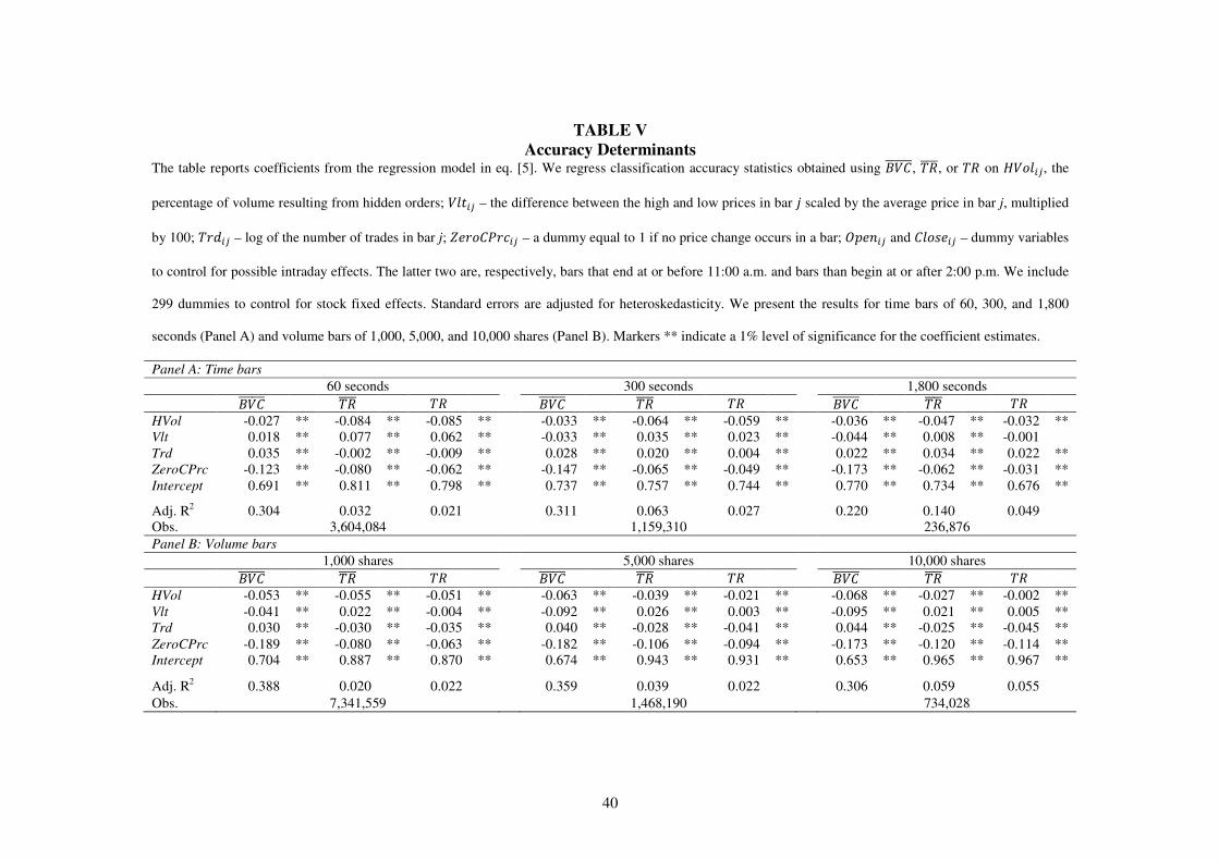
To examine accuracy across a representative subset of time bars, in Panel A of Table V,

we report regression results for bars of 60-second, 300-second, and 1,800-second lengths.

In Panel B, we report results for volume bars of 1,000, 5,000, and 10,000 shares. Results

for the entire spectrum of time and volume bars are available upon request.

The first result to catch our attention is the difference in adjusted R2s between the 1�'222222

and the tick rule specifications. 1�'222222 R2s range from 22.0% to 38.8%, whereas 3-2222 and 3-

R2s range from 2.0% to 14.0%. These statistics imply that bulk-based classification is

markedly more affected by our control variables than tick-based classification.

[Table V here]

19 We obtain similar results when we substitute the log of traded volume for the log of the number of trades.

20 This dummy allows us to isolate the bars, in which 1�'222222 will be disadvantaged compared to 3-2222. By design,

1�'222222 relies on price changes between bars to infer trade direction. With no price change, 1�'222222 will split the

volume in a bar into equal buy and sell portions, potentially negatively affecting classification accuracy.

19

Despite explaining a smaller portion of variation in 3-2222 accuracy as compared to 1�'222222

accuracy, the explanatory variables are statistically significant in almost all specifications,

for all three methods. As predicted by ELO, the proportion of hidden volume has a negative

effect on classification accuracy. Notably, the economic magnitude of this effect varies

across methods and across bar lengths/sizes. When compared to 1�'222222 accuracy, the

accuracy of 3-2222 and 3- suffers from hidden volume more in shorter time bars, but less in

larger volume bars. This result highlights the importance of differentiating not only among

classification methods, but also among bar lengths and sizes within each method.

For all bar specifications, tick rule accuracy goes up in volatility. In the meantime, 1�'222222

accuracy declines in volatility in all bars other than the ultra-short 60-second time bar. The

latter finding may seem inconsistent with the expectation that bulk volume classification

should do better in highly volatile environments. We note that the volatility variable in the

ultra-short time bars likely proxies for the price change during the bar’s 60-second duration

rather than for volatility. Given that 1�'222222 benefits from significant price changes by design,

the positive sign of the �T� variable in ultra-short time bars should not be surprising.21

As expected, 1�'222222 accuracy benefits from a larger number of trades in both time and

volume bars. In the meantime, the results for 3-2222 and 3- are not as uniform. When we

focus on time bars, the sign of the 3#W variable varies in the length of the bar. Consistent

with expectations, tick rule accuracy declines in the number of trades in the ultra-short time

21 We confirm that the �T� variable is also positive in other ultra-short time bars (for instance, 30-second

bars). We report the results for 60-second time bars here and in the subsequent tables to match ELO, who also

work with 60-second bars.

20

bars. Yet the accuracy increases in the number of trades in the longer time bars, which is

consistent with the notion of offsetting for 3-2222 but is surprising for 3-.

In volume bars, the number of trades negatively affects the tick rule accuracy. We note

that, unlike in time bars, a larger number of trades in a volume bar does not imply higher

trading volume, but rather that trades are of smaller sizes. Prior literature does not provide a

clear expectation on the effect of trade size on trade classification. Whereas Odders-White

(2000) reports that smaller trades have lower classification accuracy, Chakrabarty et al.

(2012) find the opposite effect. Our result is more consistent with that of Odders-White’s.22

Finally, consistent with our expectations, the accuracy of all three methods is negatively

affected when the methods are applied to bars with zero price changes, although the

economic significance of this effect is lower for the tick rule.

4.5. Classification accuracy and order imbalances

Trade classification algorithms are commonly used to generate estimates of order

imbalances. In this section, we examine the effect of 1�'222222 and 3-2222 accuracy on the direction

and magnitude of order imbalance metrics.

For each stock � and bar length/size b, we compute: (i) the proportion of bars for which

the estimated direction of order imbalance equals the actual direction (order imbalance is

computed as buy share volume minus sell share volume) and (ii) the volume-adjusted

22 We are curious if our results differ from those of Chakrabarty et al. (2012) because we use a different

sample period (they use 2005, while our results in Table V are based on 2011), or because they report

univariate statistics, while we study the multivariate setting. To shed some light on the cause of this

difference, we estimate volume bar specifications of eq. [5] for 2005 data. Our findings remain the same –

smaller trades have lower classification accuracy.

21

imbalance accuracy defined as:

(#.M*�+ = 1 − 1F*\

|d�.M*�� − .M*�|�*� [6]BC

�D�

where F is the number of bars; d�.M*�� is the order imbalance in bar b estimated either with

1�'222222 or 3-2222; .M*� is the actual order imbalance in barb, and �*� is the traded volume.

In Table VI, we report the cross-sectional average statistics for select time bars (Panel

A) and volume bars (Panel B). 1�'222222� accuracy in estimating correct direction of order

imbalance varies from 52.4% for the 30-second bars to 62.9% for the 1-day bars. For

1�'2222228, the lowest accuracy is obtained with 1,000-share bars (47.6%) and the highest

accuracy is obtained with 50,000-share bars (58.9%). 3-2222 accuracy is quite stable, averaging

about 74% for time bars and 75% for volume bars. Notably, for all time and volume bars,

3-2222 provides higher accuracy of order imbalance direction than 1�'222222.23

[Table VI here]

We obtain similar results for the volume-adjusted imbalance accuracy. 1�'222222� correctly

identifies 39.5% to 59.3% of volume imbalances, and 1�'2222228 correctly identifies 42.2% to

55.6% of imbalances. In the meantime, the accuracy of 3-2222� varies between 58.4% and

23 Computation of order imbalances allows for offsetting by design (footnote 12). Therefore, we do not report

order imbalances based on 3- in this table and other tables that present imbalance-related statistics.

22

88.7%, and the accuracy of 3-22228 varies between 62.7% and 86.9%. Again, 3-2222 is markedly

more accurate than 1�'222222.24

5. Trade classification and order flow toxicity (VPIN)

ELO propose a new measure of order flow toxicity called Volume-Synchronized

Probability of Informed Trading (VPIN) as a particularly useful indicator of short-term

toxicity-driven volatility in a high-frequency environment. To compute VPIN using

traditional data, researchers need a trade classification algorithm to estimate order

imbalances; ELO use 1�'222222. Given the current market trends, VPIN may become a

frequently used tool by regulators, practitioners, and researchers (e.g., Bethel et al., 2011).

Therefore, it is a suitable empirical application of the horse race between 1�'222222 and 3-2222.25

In addition to aggregating data into bars, VPIN estimation relies on volume bucketing.

Specifically, ELO suggest grouping sequential trades into equal volume buckets of

exogenously defined sizes. For instance, daily volume of e shares may be divided into ten

equal buckets of e 10⁄ shares each. Volume bucketing reduces the impact of volatility

clustering, and the resulting time series follows a distribution that is closer to normal and is

less heteroskedastic. We note that volume bucketing and assigning trades to time and

volume bars are independent processes.

Since VPIN is designed for HFT environments, we focus on the 100 largest stocks in our

sample. We also restrict our analysis to time bars. These restrictions are necessary for the

24 The difference in misclassification magnitudes between Tables I and VI is nominal and is driven by the

construction of numerators in, respectively, eq. [3] and eq. [6]. Eq. [6] allows for a larger dispersion in the

numerator, leading to statistics of somewhat different magnitudes that those derived from eq. [3].

25 Boehmer, Grammig, and Theissen (2007) do a similar analysis of the PIN measure of Easley et al. (1996).

23

following reasons. First, computation of VPIN for infrequently traded stocks is challenging.

In such stocks, time bars with zero volume are the norm, significantly reducing a

researcher’s ability to use 1�'222222. In addition, small caps often contain time bars with just

one or a few trades, compromising the accuracy of both 1�'222222 (not designed to classify

individual trades) and 3-2222 (offsetting effects are less likely to materialize).

Second, we focus on time bars because computing VPIN with volume bars involves ad

hoc decisions such as (i) whether to include overnight returns, (ii) how to compute returns

between consecutive volume buckets filled by the same trade, and (iii) how to find a

sensible ratio between the size of the volume bar and the size of the volume bucket. ELO

also do not use volume bars for VPIN estimation. Finally, recall that data vendors such as

Bloomberg provide data in time bars but not in volume bars, and it is therefore unclear

whether examining the volume-bar VPIN is practical.

5.1 VPIN computation

Following ELO, we compute VPIN as the moving average of the absolute order

imbalance over the last volume buckets. A volume bucket is defined as a fraction (1/F)

of the average daily volume of asset �, ��$T*�. We use F = {100, 50, 25, 10}, such that

F = 100 and F = 10 give, respectively, the smallest and the largest volume buckets for

each stock.26 Using the first volume buckets, we generate the first value of VPIN and

then recursively update this value by dropping the oldest volume bucket and adding a new

volume bucket:

�)Mi*��N� = ∑ |.M�|N�D� �* ,[7] 26 Andersen and Bondarenko (2012) use k = 50, which is also the base case considered by ELO.

24

where is the number of volume buckets over which VPIN is computed; τ� � denotes the

last of the n buckets; �* is the size of the volume bucket (i.e., �$T*/F), and .M� is the order

imbalance in the τ’s bucket. In our analysis, we compute .M� in three ways: (i) using the

true direction of buys and sells from ITCH data, (ii) using 1�'222222, and (iii) using 3-2222. In the

reported results, we allow F and �to vary, but fix at 50. Our conclusions are however

robust to varying . Note that for a given F, there exists a unique VPIN series when we use

the true .M� (VPIN(true)) and when we use VPIN(3-2222). Yet when we use 1�'222222, we obtain

one VPIN series for each (F, �) combination.

In Table VII, we resume the horse race between 3-2222 and 1�'222222 in estimating order

imbalance. As in Table VI, we distinguish between the accuracy of imbalance direction and

the volume-adjusted accuracy. In Table VII however, the accuracy is measured at the

volume-bucket level rather than at the time-bar level. For 1�'222222, we report statistics for two

time bars: 60 seconds and 1,800 seconds.27

Panel A of Table VII shows that 3-2222 determines the direction of order imbalance with

75.3% accuracy for the smallest volume buckets (F = 100) and with 75.2% accuracy for

the largest buckets (F = 10). In the meantime, 1�'222222 accuracy varies from 55.5% (1,800-

second bar; F = 100) to 68.6% (60-second bar; F = 10). Overall, 3-2222 is more accurate in

estimating imbalance direction for volume buckets of any size. The volume-adjusted results

are similar (Panel B). In summary, 3-2222 again outperforms 1�'222222 across the board.

[Table VII here]

5.2 Correlations between true and estimated VPINs

27 Results for other time bar lengths are similar and are available upon request.

25

In this section, using the methodology described above we calculate VPIN series using

the actual order imbalances as well as 1�'222222-based and 3-2222-based order imbalances. In Table

VIII, we report Pearson correlations between the resulting VPIN time series. The reported

values are cross-sectional averages of the individual stock correlations.

In Panel A, we show that the correlations between VPIN(true) and VPIN(3-2222) range

from a high of 76.65% for the smallest volume bucket (F = 100) to a low of 71.09% for

the largest volume bucket (F = 10), with an average correlation of 74.57%. In Panel B, we

report uniformly lower correlations between VPIN(true) and VPIN(1�'222222). For F = 100,

these correlations are 40.78% for the 60-second time bar and 18.19% for the 1,800-second

time bar. For F = 10, similar figures are 46.89% and 31.89%. We note that there is a

substantial reduction in correlation between VPIN(true) and VPIN(1�'222222) as we increase the

time bar length while keeping F constant. This reduction is consistent with the patterns in

the accuracy of the 1�'222222 order imbalances reported in Table VII. In summary, VPIN

estimates are considerably closer to their true values when we use 3-2222 instead of 1�'222222, with

the difference in average correlations of about 40 percentage points (= 74.57% - 35.27%).

[Table VIII here]

5.3 VPIN and toxic events

VPIN’s main purpose is to detect periods of unusually high order flow toxicity.

Correlations discussed in the previous section may be suggestive of the relative accuracy of

VPIN(1�'222222) and VPIN(3-2222�, but they do not tell us which of the two VPIN estimates tracks

VPIN(true) more closely when order toxicity is high. In this section, we ask if VPIN�1�'222222� outperforms VPIN(3-2222� when it is most desirable – during periods of high toxicity.

26

As ELO point out, a toxic period must be characterized by VPIN not only achieving, but

also staying at or above, a critical level. Thus, we identify potentially toxic episodes as

periods with relatively high and persistent VPIN(true) values.28 A toxic period begins when

the empirical CDF of the VPIN(true) reaches or crosses the 0.9 percentile and ends when

the CDF falls below the 0.8 percentile.29 Additionally, we split the toxic events according

to their persistence, measured by the number of volume buckets in the event. An event is

classified as low-persistence if it is at or below the 25 percentile of the distribution, mid-

persistence if it is between the 25 and the 75 percentiles, and high-persistence if it is at or

above the 75 percentile.

In Table IX, we report the percentage of true toxic events, as flagged by the VPIN(true),

that are correctly identified by VPIN(1�'222222) and VPIN(3-2222). Our main interest is in the

highly persistent events (in bold font), but we report results for the other two groups for

completeness. As in other tables in this section, we report 1�'222222 results for the 60-second

and 1,800-second time bars.

[Table IX here]

Table IX shows that while VPIN(1�'222222) achieves its highest concurrence with VPIN(true) at

about 68% when we use 60-second time bars, VPIN(3-2222) fares much better with

concurrence rates above 91%. More generally, the consensus between VPIN(3-2222) and

28 We are not aware of any systematic toxic events during our sample period. Therefore, we do not expect our

analysis to find historical or global maxima for VPIN. Rather, our analysis should identify local maxima, i.e.,

relatively more toxic periods for each asset between May and July 2011.

29 We have examined alternative endings for toxic periods. Specifically, we allowed the VPIN CDF to fall

below 0.9 or below 0.85. Our conclusions are similar and available upon request.

27

VPIN(true) is uniformly higher than the consensus between VPIN(1�'222222) and VPIN(true)

for all volume buckets, all time bars, and all levels of persistence.

6. Robustness

6.1. Dispersion of classification metrics

Results reported so far are based on the means of accuracy ratios. Although the means

suggest that 3-2222 provides more accurate classifications than 1�'222222, we have not yet discussed

the possibility that 1�'222222 may be more stable.

To shed more light on the issue of stability, in Table X we report the cross-sectional

medians of the inter-quartile range (IQR) statistics for 1�'222222, 3-2222, and 3-. First, we compute

IQRs for all stocks (Panel A), then only for large caps (Panel B), and finally for all stocks

while eliminating bars with less than two trades (Panel C). We report the results for 1,800-

second time bars and 5,000-share volume bars, but the results for the full spectrum of bars

are similar. The results indicate that 3-2222 statistics have considerably lower dispersion when

compared to the alternatives. Namely, in all panels and for both time and volume bars,

IQRs for 3-2222 are notably lower than those for 1�'222222 and 3-.

[Table X here]

To further explore the distributional properties of classification accuracy, in Figure 1 we

report the empirical distribution of accuracy ratios in the form of CDFs. Visually, when the

line representing a classification method lies underneath (or to the right of) the line

representing another method, the former method is preferred. For example, Figure 1a

indicates for time bars that 3-2222 statistics are superior to 1�'222222 statistics across most of the

28

distribution, as the solid line that represents 3-2222 lies mainly underneath and to the left of the

broken line representing 1�'222222.

[Figure 1 here]

6.2. Classification accuracy and the likelihood of one-sided order flow

Earlier, we showed that 3-2222 is more accurate than 1�'222222 for order imbalance

measurement. We realize that the main premise of bulk-based classification is that large

order imbalances coincide with large changes in prices. The lower accuracy of 1�'222222 may

therefore arise from bars in which price changes are close to zero. In this section, we gauge

the accuracy of 1�'222222 and 3-2222 conditional on the estimated probability of one-sided order

flow as given by )# = �?∆� �∆�⁄ @ in eq. [1]. For each stock and bar length/size, we split

bars into three subsets according to )#: 0.3 ≤ )# ≤ 0.7 (low); 0.7 < )# ≤ 0.9 or 0.7 ≤1 − )# ≤ 0.9 (mid), and )# > 0.9 or 1 − )# > 0.9 (high). Our findings for low and high

subsets are in Table XI.

For both time bars (Panel A) and volume bars (Panel B), we confirm our expectations

that 1�'2222222is the least accurate when applied to bars with low probability of one-sided order

flow. Meanwhile, 3-2222 performance for such bars is notably better. More importantly, even

when applied to the bars with high )#, 3-2222 never underperforms 1�'2222222. [Table XI here]

6.3. Alternative tests of order imbalance accuracy

In section 4.5, we show that 3-2222 outperforms 1�'2222222 in estimating order imbalances. In a

series of robustness tests (available upon request), we find that correlations between d�.M� and .M are always higher when we use 3-2222 instead of 1�'2222222. The differences between the

29

two classification methodologies are most pronounced for longer (larger) time (volume)

bars. For example, for the longest (one trading day) time bars, correlation between d�.M� and .M is 68.36% using 3-2222 and 33.34% using 1�'2222222. For the largest (50,000-share) volume

bars, the correlations are 73.06% using 3-2222 and 45.33% using 1�'2222222. Furthermore, in a

pooled regression framework, when .M is regressed on d�.M�, the adjusted R2s are

uniformly larger (often, twice as large) in the 3-2222 specifications.

6.4 Type II error

In section 5.4, we ask how many highly toxic events identified by VPIN(true) are also

detected by VPIN(3-2222) and VPIN(1�'222222). In this section, we look at this issue from the

opposite angle and ask how many events identified as highly toxic by VPIN(3-2222) and

VPIN(1�'222222) are actually not highly toxic according to VPIN(true).

Table XII shows that 3-2222 generates fewer errors in identifying highly toxic events than

does 1�'222222. For F = 10 buckets, 3-2222 over-detects 10.6% of the highly toxic events, while

1�'222222 over-detects 22.6% to 29.5% of the events, depending on the time bar used. The

differences are larger for smaller volume bucket sizes.

[Table XII here]

6.5. INET v. TAQ trade sequences and prices

INET order data allow us to compare 1�'222222 and 3-2222 classifications to true classification,

but these data come with a notable limitation. While we observe signed trades on the INET

platform, we do not observe trades that execute elsewhere. Although this issue is not unique

to our study, observing all transactions is perhaps particularly important for trade

classification. In today’s ultra-fast markets, distances between stock exchanges and the

30

consolidated tape aggregator (also known as the Security Information Processor or SIP)

have become particularly important. For example, if a trade report from exchange A takes 4

milliseconds (ms) to travel to SIP, while a trade report from exchange B only takes 1 ms to

make the same trip, a trade that executes on A 1 ms before a trade on B will be reported in

TAQ as if it executed 2 ms after the trade on B. Given this example, and because 3-2222 classification directly depends on proper trade and price sequencing, 3-2222 accuracy may

suffer when applied to the consolidated data.

We address this issue by examining the accuracy of 3-2222�3(n� – the tick rule applied to

TAQ trade and price sequences. We still need a benchmark for this analysis. To obtain this

benchmark, we identify INET trades among TAQ trades as follows: we take INET trades of

100 and more shares30 and match them to TAQ trades by stock, date, reporting facility,

timestamp, price, and size. We allow a lead/lag of five seconds between INET and TAQ

timestamps. Most matches occur when we use one-second leads/lags. After 2006, trades in

NASDAQ listed stocks that execute on the INET platform are reported to TAQ exclusively

through the Trade Reporting Facility (TRF, TAQ exchange symbol ‘Q’).31 Our match

success rate is about 97%.

Once the trades are matched, we compare true trade classification of INET trades to

classification derived by applying 3-2222�3(n�. In addition, we compute 1�'222222��3(n� using

TAQ price changes between time bars and compare resulting classification to true

30 While INET data contain all trades, TAQ data omit odd lots – trades of fewer than 100 shares. In

unreported results, we compute 1�'222222 and 3-2222 accuracies for the INET trades while excluding odd lots. The

results are very similar to those reported in Table I and are available upon request.

31 We thank Frank Hatheway, NASDAQ’s chief economist, for information on trade reporting venues.

31

classification. We note that we cannot effectively use TAQ prices to estimate 1�'2222228�3(n� because volume bars would include only matched INET trades, rather than all TAQ trades.

The results of this exercise are in Table XIII. The data show that 3-2222�3(n� classification

is never worse than 3-2222�Mid3� classification. Furthermore, 3-2222 continues to outperform

1�'222222. It therefore appears that our main results derived from ITCH data apply even when

we account for trade reporting latencies.

[Table XIII here]

A somewhat separate concern arises from the fact that INET prices may not successfully

proxy for the price patterns in the entire market. We concur that because 1�'222222 accuracy

depends on observing correct price changes, it is important to check if INET prices and

market-wide prices are truly interchangeable. A priori, INET prices should closely co-move

with TAQ prices because of order protection rules, smart order routing, and inter-market

arbitrage. We examine if this reasoning is correct using consolidated TAQ trades for the

100 largest stocks in our sample.

We use trades from all markets and filter the data following Hendershott and Moulton

(2011). For a given time bar length, we measure the consolidated TAQ volume and INET

volume as well as the TAQ-based and INET-based prices changes. We exclude time bars

with no volume in either TAQ or INET.32 Finally, we compute VPIN(1�'222222) as in the earlier

sections but using (i) price changes from INET data and (ii) price changes from TAQ data

32 For a given bar, INET volume may be positive while TAQ volume is zero if INET trades are odd lots,

which TAQ does not report.

32

to classify INET volume. In Table XIV, we report cross-sectional correlations between

TAQ and INET price changes and between VPIN(1�'222222) series of types (i) and (ii) above.

[Table XIV here]

Our results show that INET prices proxy for TAQ prices very well. In the 30-second

time bars, the correlation between TAQ and INET price changes is greater than 71%. For

the 1,800-second time bars, the correlation is 95.8%. More importantly, the correlation

between the TAQ-based and INET-based VPIN(1�'222222) is always greater than 94%.

7. Conclusions

Traditional trade classification algorithms are becoming more challenging to implement

in today’s high frequency markets characterized by big data. In a recent study, ELO

propose a bulk-volume classification method (BVC) that may overcome the data processing

hurdles if a researcher uses vendor-compressed data (e.g., Bloomberg data). Using data on

index and commodity futures, ELO conclude that the BVC algorithm is superior to the tick-

based algorithms not only in resource requirements, but also in accuracy.

We test BVC accuracy when applied to equities and compare it to the simple tick rule

(TR). We find that TR has higher accuracy than BVC, and that misclassification increases

by 7.4 to 16.3 percentage points (or 46% to 291%) when switching from TR to BVC.

Meanwhile, BVC allows for significant time savings when applied to vendor-compressed

data (BVC takes 1% of the time TR takes), and for notable time savings when applied to

traditional tick-level data such as TAQ (BVC takes about 25% of the time TR takes).

We examine temporal change in classification accuracy for TR by comparing our 2011

results with a matched sample from 2005 and find that indeed TR accuracy declined, but

33

only marginally, from 77.8% in 2005 to 77.0% in 2011. We also find that TR outperforms

BVC in estimating the direction and accuracy of order imbalances.

Finally, we ask if differences in classification accuracy between the bulk-based and the

tick-based methods may significantly affect empirical applications. To answer this

question, we apply both methods to compute VPIN. We find that TR, again, fares better

than BVC when used to identify periods of high and persistent order flow toxicity.

Our results are robust to a number of checks such as excluding small and medium caps,

excluding bars with zero price changes and bars with low probability of one-sided order

flow. We obtain similar results when we use Student’s t-distribution or the empirical

distribution instead of the standard normal distribution. In addition, the results are robust to

trade reporting latencies typical for contemporary markets. Our findings should be useful to

researchers by quantifying the trade-off between accuracy and computational efficiency in

choosing a trade classification algorithm.

34

References

Andersen, T. G. and O. Bondarenko, 2012, VPIN and the flash crash, Journal of Financial

Markets, forthcoming.

Bethel, E. W., D. Leinweber, O. Rübel, and K. Wu, 2011, Federal Market Information

Technology in the Post Flash Crash Era: Roles for Supercomputing, Lawrence Berkeley

National Laboratory, Working paper.

Boehmer, E., J. Grammig, and E. Theissen, 2007, Estimating the probability of informed

trading: does trade misclassification matter? Journal of Financial Markets 10, 26-47.

Brogaard, J., T. Hendershott, and R. Riordan, 2012, High frequency trading and price

discovery, SSRN working paper.

Chakrabarty, B., B. Li, V. Nguyen, and R. Van Ness, 2007, Trade classification algorithms

for electronic communications network trades, Journal of Banking and Finance 31,

3806-3821.

Chakrabarty, B., P. Moulton, and A. Shkilko, 2012, Short sales, long sales, and the Lee-

Ready trade classification algorithm revisited, Journal of Financial Markets 15, 467-

491.

Chordia, T., and A. Subrahmanyam, 2004, Order imbalance and individual stock returns:

Theory and evidence, Journal of Financial Economics 72, 485-518.

Easley, D., N. Kiefer, M. O’Hara, and J. Paperman, 1996, Liquidity, information, and

infrequently traded stocks, Journal of Finance 51, 1405-1436.

Easley, D., M. López de Prado, and M. O’Hara, 2012a, Bulk classification of trading

activity. Johnson School Research Paper Series #8-2012.

35

Easley, D., M. López de Prado, and M. O’Hara, 2012b, Flow toxicity and liquidity in a

high-frequency world, Review of Financial Studies 25, 1457-1493.

Ellis, K., R. Michaely, and M. O’Hara, 2000, The accuracy of trade classification rules:

Evidence from Nasdaq, Journal of Financial and Quantitative Analysis 35, 529-551.

Gai, J., C. Yao, and M. Ye, 2012, The externality of high frequency trading. SSRN Working

Paper.

Hasbrouck, J., 1991, Measuring the information content of stock trades, Journal of Finance

46, 179-207.

Hasbrouck, J., and G. Saar, 2012, Low-latency trading, SSRN Working Paper.

Hendershott T. and P. Moulton, 2011, Automation, speed, and stock market liquidity: The

NYSE’s hybrid, Journal of Financial Markets 14, 568-604.

Holden, C. and S. Jacobsen, 2012, Liquidity measurement problems in fast, competitive

markets: Expensive and cheap solutions, SSRN Working Paper.

Huang, R., and H. Stoll, 1997, The components of the bid-ask spread: a general approach,

Review of Financial Studies 10, 995-1034.

Lee, C. M. C., and M. Ready, 1991, Inferring trade direction from intraday data, Journal of

Finance 46, 733-747.

Odders-White, E., 2000, On the occurrence and consequences of inaccurate trade

classification, Journal of Financial Markets 3, 259-286.

O’Hara, M., C. Yao, and M. Ye, 2012, What’s not there: The odd-lot bias in TAQ data,

SSRN working paper.

36

TABLE I

Classification Accuracy: opq222222, rs2222, and rs We report accuracy ratios for the tick rule, 3-, without offsetting (Panel A), the 1�'222222 algorithm, and the tick rule with offsetting, 3-2222, (Panel B) for a sample of

300 stocks traded on INET in May-July 2011 and a matched sample for May-July 2005. 1�'222222 and 3-2222 are computed using time bars (1�'222222L and 3-2222L) and volume

bars without overnight returns (1�'222222t and 3-2222t). Accuracy ratios are cross-sectional averages of the percentage of volume correctly classified by each algorithm.

Non-parametric one-sided Wilcoxon rank-sum tests gauge for differences between the three classification rules. Boldface statistics in the 1�'222222 columns indicate

that 1�'222222 is more accurate than 3- at 1% level of significance. ** indicates that 3-2222 is more accurate than 1�'222222 at 1% level of significance.

Panel A: Tick rule without offsetting, 3-

2011: 0.770 2005: 0.778

Panel B: BVC and TR with offsetting, 1�'222222 and 3-2222

time bars volume bars

2011 2005 2011 2005

bar length, sec. 1�'222222� 3-2222� 1�'222222� 3-2222� bar size, sh. 1�'2222228 3-22228 1�'2222228 3-22228

1 0.643 0.775 ** 0.623 0.779 ** 1,000 0.711 0.813 ** 0.679 0.807 **

2 0.649 0.777 ** 0.627 0.780 ** 2,000 0.740 0.836 ** 0.710 0.825 **

3 0.653 0.777 ** 0.629 0.780 ** 3,000 0.753 0.851 ** 0.724 0.838 **

5 0.659 0.779 ** 0.633 0.781 ** 4,000 0.761 0.861 ** 0.732 0.846 **

10 0.671 0.783 ** 0.640 0.783 ** 5,000 0.765 0.869 ** 0.738 0.853 **

30 0.698 0.792 ** 0.657 0.790 ** 6,000 0.769 0.875 ** 0.742 0.859 **

60 0.718 0.802 ** 0.673 0.796 ** 7,000 0.771 0.881 ** 0.745 0.864 **

300 0.765 0.839 ** 0.718 0.822 ** 8,000 0.773 0.885 ** 0.747 0.868 **

1,800 0.794 0.889 ** 0.755 0.865 ** 9,000 0.775 0.889 ** 0.750 0.872 **

3,900 0.797 0.908 ** 0.762 0.884 ** 10,000 0.776 0.892 ** 0.751 0.875 **

7,800 0.794 0.923 ** 0.765 0.900 ** 30,000 0.781 0.923 ** 0.761 0.906 **

23,400 0.781 0.944 ** 0.759 0.922 ** 50,000 0.778 0.935 ** 0.763 0.918 **

37

TABLE II

Changes in Classification Accuracy: 2011 v. 2005 The table reports changes in accuracy of the conventional trade-level tick rule, 3-, (Panel A), the 1�'222222

algorithm and the tick rule computed to allow for offsetting, 3-2222, (Panel B). We compute the changes between

the 2011 sample and the 2005 matched sample and report cross-sectional change statistics. Asterisks ** and *

denote instances whereby the change is statistically significant at the 1% and 5% level respectively.

Panel A: ∆3-

-0.008*

Panel B: ∆1�'222222 and ∆3-2222

time bars volume bars

bar length, sec. ∆1�'222222� ∆3-2222� bar size, # sh. ∆1�'2222228 ∆3-22228

1 0.021 ** -0.004 * 1,000 0.032 ** 0.006 **

2 0.026 ** -0.002 2,000 0.030 ** 0.013 **

3 0.040 ** 0.003 3,000 0.029 ** 0.016 **

5 0.045 ** 0.006 * 4,000 0.029 ** 0.017 **

10 0.047 ** 0.017 ** 5,000 0.028 ** 0.017 **

30 0.039 ** 0.023 ** 6,000 0.027 ** 0.017 **

60 0.035 ** 0.024 ** 7,000 0.026 ** 0.017 **

300 0.029 ** 0.024 ** 8,000 0.027 ** 0.017 **

1,800 0.022 ** 0.021 ** 9,000 0.025 ** 0.006 **

3,900 0.021 ** -0.004 * 10,000 0.026 ** 0.013 **

7,800 0.026 ** -0.002 30,000 0.020 ** 0.016 **

23,400 0.040 ** 0.003 50,000 0.015 ** 0.017 **

38

TABLE III

Data Compression and Processing Time Panel A contains statistics on the levels of compression achieved by aggregating tick data into time and

volume bars. The level of compression is computed as 1 minus the ratio of time/volume bars needed to

classify volume traded during the 3-month sample period to the total number of trades in this period. We do

not count zero-volume time bars. Panel B reports processing times (in seconds) required to sign volume in a

sample stock (Microsoft Corp.: MSFT, in June 2011) depending on data availability. We consider two

scenarios: (i) a researcher is working with tick data and (ii) a researcher is working with bar data. Processing

time includes (a) time to upload tick (bar) data into Matlab, (b) time to aggregate tick data into 3,900-second

time bars, (c) time to sign volume either based on tick data or on bar data. Our results do not change

qualitatively if we use time bars of other lengths or if we use volume bars.

Panel A: Data compression

time bars volume bars

bar length, sec. bar size, # sh.

1 0.5015 1,000 0.8709

5 0.5703 3,000 0.9570

30 0.6964 5,000 0.9742

300 0.8782 7,000 0.9816

1,800 0.9647 9,000 0.9857

3,900 0.9819 10,000 0.9871

7,800 0.9905 30,000 0.9957

23,400 0.9968 50,000 0.9974

Panel B: Processing time, seconds (trades for MSFT in June 2011)

3-2222 (tick data) 1�'222222 (tick data) 1�'222222 (bar data)

upload tick data 12.531 12.531

upload bar data 0.005

aggregate into bars 0.204

sign volume 0.859 0.010 0.010

total time 13.389 12.724 0.015

39

TABLE IV

Classification Accuracy: Large v. Small Stocks The table reports the accuracy ratios for 3- (Panel A), 1�'222222, and 3-2222 (Panel B). 1�'222222 and 3-2222 are computed using time bars (1�'222222L and 3-2222L) and volume bars

without overnight returns (1�'222222t and 3-2222t). We report the statistics for large caps (100 stocks in the large market capitalization group) and for small caps (100

stocks in the small group). Accuracy ratios represent cross-sectional averages of the percentage of volume correctly classified by each algorithm. For 1�'222222 and

3-2222, we use time bar lengths from one second to one full trading day and volume bar sizes from 1,000 to 50,000 shares. We report two statistical tests (non-

parametric one-sided Wilcoxon rank-sum tests) to gauge differences between the three trade classification methods. Boldface statistics in the 1�'222222 columns are

associated with the first test and indicate that 1�'222222 provides more accurate classifications than the conventional 3- at the 1% level of statistical significance.

Marker ** associated with the second test indicates that 3-2222 provides more accurate classifications than 1�'222222 at 1% level of significance.

Panel A: Tick rule without offsetting, 3-

large caps: 0.768 small caps: 0.777

Panel B: BVC and TR with offsetting, 1�'222222 and 3-2222

time bars volume bars

large caps small caps large caps small caps

bar length, sec. 1�'222222� 3-2222� 1�'222222� 3-2222� bar size, sh. 1�'2222228 3-22228 1�'2222228 3-22228

1 0.671 0.772 ** 0.624 0.781 ** 1,000 0.716 0.801 ** 0.695 0.820 **

5 0.695 0.778 ** 0.634 0.783 ** 3,000 0.763 0.840 ** 0.736 0.855 **

30 0.750 0.802 ** 0.659 0.788 ** 5,000 0.775 0.859 ** 0.750 0.872 **

300 0.815 0.876 ** 0.716 0.811 ** 7,000 0.782 0.871 ** 0.757 0.884 **

1,800 0.816 0.929 ** 0.801 0.887 ** 9,000 0.785 0.880 ** 0.761 0.890 **

3,900 0.808 0.945 ** 0.780 0.872 ** 10,000 0.786 0.884 ** 0.763 0.894 **

7,800 0.799 0.955 ** 0.784 0.890 ** 30,000 0.791 0.917 ** 0.772 0.923 **

23,400 0.773 0.968 ** 0.787 0.918 ** 50,000 0.789 0.929 ** 0.767 0.935 **

40

TABLE V

Accuracy Determinants The table reports coefficients from the regression model in eq. [5]. We regress classification accuracy statistics obtained using 1�'222222, 3-2222, or 3- on S�$T*+, the

percentage of volume resulting from hidden orders; �T�*+ – the difference between the high and low prices in bar a scaled by the average price in bar j, multiplied

by 100; 3#W*+ – log of the number of trades in bar j; �"#$')#�*+ – a dummy equal to 1 if no price change occurs in a bar; ." *+ and 'T$K"*+ – dummy variables

to control for possible intraday effects. The latter two are, respectively, bars that end at or before 11:00 a.m. and bars than begin at or after 2:00 p.m. We include

299 dummies to control for stock fixed effects. Standard errors are adjusted for heteroskedasticity. We present the results for time bars of 60, 300, and 1,800

seconds (Panel A) and volume bars of 1,000, 5,000, and 10,000 shares (Panel B). Markers ** indicate a 1% level of significance for the coefficient estimates.

Panel A: Time bars

60 seconds 300 seconds 1,800 seconds

1�'222222 3-2222 3- 1�'222222 3-2222 3- 1�'222222 3-2222 3-

HVol -0.027 ** -0.084 ** -0.085 ** -0.033 ** -0.064 ** -0.059 ** -0.036 ** -0.047 ** -0.032 ** Vlt 0.018 ** 0.077 ** 0.062 ** -0.033 ** 0.035 ** 0.023 ** -0.044 ** 0.008 ** -0.001 Trd 0.035 ** -0.002 ** -0.009 ** 0.028 ** 0.020 ** 0.004 ** 0.022 ** 0.034 ** 0.022 ** ZeroCPrc -0.123 ** -0.080 ** -0.062 ** -0.147 ** -0.065 ** -0.049 ** -0.173 ** -0.062 ** -0.031 ** Intercept 0.691 ** 0.811 ** 0.798 ** 0.737 ** 0.757 ** 0.744 ** 0.770 ** 0.734 ** 0.676 **

Adj. R2 0.304 0.032 0.021 0.311 0.063 0.027 0.220 0.140 0.049 Obs. 3,604,084 1,159,310 236,876

Panel B: Volume bars

1,000 shares 5,000 shares 10,000 shares

1�'222222 3-2222 3- 1�'222222 3-2222 3- 1�'222222 3-2222 3-

HVol -0.053 ** -0.055 ** -0.051 ** -0.063 ** -0.039 ** -0.021 ** -0.068 ** -0.027 ** -0.002 ** Vlt -0.041 ** 0.022 ** -0.004 ** -0.092 ** 0.026 ** 0.003 ** -0.095 ** 0.021 ** 0.005 ** Trd 0.030 ** -0.030 ** -0.035 ** 0.040 ** -0.028 ** -0.041 ** 0.044 ** -0.025 ** -0.045 ** ZeroCPrc -0.189 ** -0.080 ** -0.063 ** -0.182 ** -0.106 ** -0.094 ** -0.173 ** -0.120 ** -0.114 ** Intercept 0.704 ** 0.887 ** 0.870 ** 0.674 ** 0.943 ** 0.931 ** 0.653 ** 0.965 ** 0.967 **

Adj. R2 0.388 0.020 0.022 0.359 0.039 0.022 0.306 0.059 0.055

Obs. 7,341,559 1,468,190 734,028

41

TABLE VI

Classification Accuracy and Order Imbalance The table reports the accuracy of order imbalance statistics estimated using 1�'222222 and 3-2222. In Panel A, we use time

bars, while Panel B contains results for volume bars. We report two imbalance statistics: (i) the number of bars, for

which the algorithms correctly identify imbalance direction, and (ii) the volume-based accuracy measure. Asterisk

** denotes instances whereby the difference between 1�'222222 and 3-2222 estimates is statistically significant at the 1%

level.

% bars correctly classified imbalance accuracy

1�'222222 3-2222 1�'222222 3-2222

Panel A: time bars

30 0.524 ** 0.743 0.395 ** 0.584

60 0.539 ** 0.739 0.436 ** 0.604

300 0.572 ** 0.726 0.529 ** 0.677

1,800 0.596 ** 0.725 0.588 ** 0.777

3,900 0.607 ** 0.731 0.593 ** 0.817

7,800 0.611 ** 0.742 0.588 ** 0.847

23,400 0.629 ** 0.759 0.561 ** 0.887

Panel B: volume bars

1,000 0.476 ** 0.745 0.422 ** 0.627

3,000 0.542 ** 0.747 0.506 ** 0.702

5,000 0.561 ** 0.750 0.531 ** 0.738

7,000 0.572 ** 0.752 0.543 ** 0.762

9,000 0.576 ** 0.755 0.549 ** 0.777

10,000 0.582 ** 0.755 0.552 ** 0.784

50,000 0.589 ** 0.762 0.556 ** 0.869

42

TABLE VII

Order Imbalance Accuracy in Volume Buckets The table contains cross-sectional order imbalance accuracy statistics for 1�'222222 and 3-2222. We examine the direction

(Panel A) and signed magnitude (Panel B) of order imbalances on the volume bucket level. We consider two time

bar resolutions for 1�'222222: 60 seconds and 1,800 seconds. The stock-specific size of a volume bucket is defined as

the average daily share volume divided by F = {100, 50, 25, 10}, with F = 100 capturing the smallest buckets,

and F = 10 capturing the largest buckets. In Panel A, the accuracy is the proportion of volume buckets for which

the estimated direction of the order imbalance coincides with the actual direction of order imbalance. In Panel B,

accuracy is computed as in eq. [6], but using τ as the index for volume buckets rather than the index for time/size

bars.

volume bucket size F = 100 (small) F = 50 F = 25 k=10 (large)

Panel A: Imbalance direction

3-2222 0.753 0.750 0.749 0.752 1�'222222 (60 sec.) 0.674 0.682 0.685 0.686

1�'222222 (1,800 sec.) 0.555 0.574 0.594 0.619

Panel B: Imbalance magnitude

3-2222 0.707 0.762 0.810 0.861 1�'222222 (60 sec.) 0.657 0.725 0.779 0.832 1�'222222 (1,800 sec.) 0.507 0.568 0.619 0.685

43

TABLE VIII

Correlations between VPIN series The table reports cross-sectional linear correlations between the VPIN series obtained using true order imbalances

from INET (VPIN(true)) and the VPIN series obtained using the order imbalances estimated 3-2222 (Panel A) and

1�'222222 with time bars (Panel B). We also report the cross-sectional correlations between the CDF of the true VPIN

and the CDF of the 3-2222-based VPIN and the 1�'222222-based VPIN. We consider two time bar resolutions for 1�'222222: 60

seconds and 1,800 seconds. The stock-specific size of a volume bucket is defined as the average daily share

volume divided by F = {100, 50, 25, 10}, with F = 100 capturing the smallest buckets, and F = 10 capturing the

largest buckets. For 3-2222, the results are independent of the length of the time bar. We use only the 100 largest

sample stocks. Finally, we report the proportion of stocks for which the correlation is statistically significant at the

1% level.

F � VPIN signif. at 1% CDF(VPIN) signif. at 1%

Panel A: Correlations between VPIN (true) and VPIN (3-2222)

100 (small) 0.7665 100 0.7282 100 50 0.7602 100 0.7122 100 25 0.7454 100 0.6954 100

10 (large) 0.7109 99 0.6592 98

mean 0.7457 0.6987

Panel B: Correlations between VPIN (true) and VPIN (1�'222222)

100 (small) 60 sec. 0.4078 100 0.3675 99

1,800 sec. 0.1819 91 0.1316 88

50 60 sec. 0.4515 99 0.4054 99

1,800 sec. 0.2207 87 0.1692 87

25 60 sec. 0.4755 95 0.4276 95

1,800 sec. 0.2623 86 0.2130 89

10 (large) 60 sec. 0.4689 95 0.4042 96

1,800 sec. 0.3189 79 0.2590 76

mean 0.3527 0.3026

44

TABLE IX

Accuracy of Toxic Event Identification The table reports cross-sectional average proportion of toxic events flagged by the true VPIN that are also detected

by the 1�'222222-based VPIN (with time bars) and the 3-2222-based VPIN. A toxic event begins when the CDF of the true

VPIN is at or above the 0.9 percentile and ends when the CDF falls below the 0.8 percentile. We split toxic events

into three subsets according to persistence. Persistence is measured as the number of buckets in each event.

Persistence is ‘low’ when it is at or below the 25 percentile of the empirical distribution of persistence of all toxic

events in a given volume bucket size; ‘mid’ when it is between the 25 and 75 percentiles; and ‘high’ when it is at

or above the 75 percentile. Highly persistent toxic events (in bold) are the ones we focus on, as they are most

likely to be truly toxic. We consider two time bar resolutions for 1�'222222: 60 seconds and 1,800 seconds. The stock-

specific size of a volume bucket is defined as the average daily share volume divided by F = {100, 50, 25, 10}, with F = 100 capturing the smallest buckets, and F = 10 capturing the largest buckets. We limit this analysis to

the 100 largest stocks.

% of correctly identified toxic events F persistence # events 1�'222222 (60 sec.) 1�'222222 (1,800 sec.) 3-2222

100 (small) low 484 0.240 0.184 0.395 mid 913 0.392 0.315 0.717

high 466 0.648 0.545 0.931

50 low 254 0.283 0.213 0.390 mid 488 0.389 0.336 0.652 high 258 0.678 0.543 0.926

25 low 154 0.299 0.260 0.474 mid 265 0.377 0.313 0.596 high 162 0.617 0.537 0.914

10 (large)

low 82 0.317 0.293 0.366

mid 150 0.360 0.353 0.607

high 79 0.684 0.620 0.924

45

TABLE X

Dispersion of Estimates The table reports the inter-quartile range (IQR) of the empirical distribution of the accuracy ratios for 1�'222222, 3-2222,

and 3-. We compute IQRs for time bars of 1,800 seconds (30 minutes) and volume bars of 5,000 shares. In Panel

A, we report statistics for all bars and all stocks. In Panel B, we report statistics for all bars and only the 100

largest stocks. In Panel C, we report statistics for the bars with at least two trades per bar and all stocks.

1,800-second time bars 5,000-share volume bars

Panel A: All stocks

1�'222222 0.206 1�'222222 0.237

3-2222 0.156 3-2222 0.137

3- 0.203 3- 0.192

Panel B: Large caps

1�'222222 0.177 1�'222222 0.220

3-2222 0.080 3-2222 0.142

3- 0.106 3- 0.193

Panel C: Bars with at least two trades

1�'222222 0.205 1�'222222 0.236

3-2222 0.155 3-2222 0.137

3- 0.203 3- 0.192

46

TABLE XI

Classification Accuracy and One-Sided Order Flow The table reports the accuracy of order imbalance statistics estimated using 1�'222222 and 3-2222 conditional on the

probability of one sided order flow given by )# = �?∆� �∆�⁄ @ in eq. [1]. For each stock and bar length/size, we

split bars into three subsets according to )#: (i) 0.3 ≤ )# ≤ 0.7 (low); 0.7 < )# ≤ 0.9 or 0.7 ≤ 1 − )# ≤ 0.9

(mid), and )# > 0.9 or 1 − )# > 0.9 (high). In Panel A, we use time bars, while Panel B contains results for

volume bars. We report two imbalance statistics: (i) the number of bars for which the algorithms correctly identify

imbalance direction, and (ii) the volume-based accuracy measure. Asterisk ** denotes instances whereby the

difference between 1�'222222 and 3-2222 estimates is statistically significant at the 1% level.

% bars correctly classified imbalance accuracy

1�'222222 3-2222 1�'222222 3-2222 low high low high low high low high

Panel A: time bars

30 0.408 0.818 0.715** 0.818 0.195 0.561 0.475** 0.629** 60 0.435 0.814 0.712** 0.817 0.246 0.538 0.490** 0.633**

300 0.488 0.795 0.700** 0.814** 0.417 0.446 0.563** 0.668** 1,800 0.525 0.771 0.701** 0.803** 0.617 0.331 0.699** 0.759**

Panel B: volume bars

1,000 0.303 0.764 0.733** 0.783** 0.378 0.432 0.612** 0.658** 3,000 0.397 0.763 0.733** 0.793** 0.528 0.370 0.689** 0.730** 5,000 0.432 0.755 0.735** 0.796** 0.587 0.337 0.726** 0.764**

10,000 0.466 0.745 0.734** 0.808** 0.652 0.299 0.771** 0.807**

47

TABLE XII

Highly Toxic Events Identification: Type II error The table reports cross-sectional average proportion of highly toxic events that are not flagged by the true VPIN

but flagged by the 1�'222222-based VPIN (with time bars) and the 3-2222-based VPIN – the type II error. A toxic event

begins when the CDF of the true VPIN is at or above the 0.9 percentile and ends when the CDF falls below the 0.8

percentile. We split toxic events into three subsets according to persistence. Persistence is measured as the number

of buckets in each event. Persistence is ‘low’ when it is at or below the 25 percentile of the empirical distribution

of persistence of all toxic events in a given volume bucket size; ‘mid’ when it is between the 25 and 75 percentiles;

and ‘high’ when it is at or above the 75 percentile. We report the results for only the highly toxic events. We

consider two time bar resolutions for 1�'222222: 60 seconds and 1,800 seconds. The stock-specific size of a volume

bucket is defined as the average daily share volume divided by F = {100, 50, 25, 10}, with F = 100 capturing the

smallest buckets, and F = 10 capturing the largest buckets. We limit this analysis to the 100 largest stocks.

incorrectly identified toxic events

1�'222222 (60 sec.) 1�'222222 (1,800 sec.) 3-2222 F # events % error # events % error # events % error

100 (small) 361 0.251 386 0.350 511 0.082 50 193 0.201 214 0.341 302 0.073 25 108 0.168 120 0.308 152 0.079

10 (large) 54 0.226 61 0.295 85 0.106

48

TABLE XIII

Classification Rules Applied to TAQ Trade Sequences The table reports cross-sectional average accuracy ratios for 1�'222222 and 3-2222 using (a) INET trades and prices and (b)

consolidated TAQ trades and prices. We match INET trades for 100 or more shares with TAQ trades executed on

NASDAQ based on stock, date, reporting facility, timestamp, price, and size. We allow for a 5-second lead/lag in

the time match. The sample is restricted to the 100 largest stocks. We compute the accuracy ratios by comparing

3-2222�Mid3� and 3-2222�3(n� classifications with the true direction for the matched INET trades. We compute the

accuracy of 1�'222222�3(n� using TAQ prices to define price changes between time bars, and using INET prices to

define price changes between volume bars. In volume bar construction, we are restricted to matched INET trades,

therefore we are unable to compute 1�'222222�3(n� for volume bars. We report four time bar resolutions: 30, 60, 300,

and 1,800 seconds, and four volume bar resolutions: 1,000, 3,000, 5,000 and 10,000 shares. We use non-

parametric Wilcoxon rank-sum tests to examine null hypotheses that (i) the median accuracy of 3-2222�Mid3� and

3-2222�3(n� are equal and (ii) the median accuracy of 1�'222222�Mid3� and 1�'222222�3(n� are equal. Asterisks ** and *

denote statistical significance at the 1% and 5% level.

1�'222222�3(n� 1�'222222�Mid3� 3-2222�3(n� 3-2222�Mid3� Panel A: time bars

30 0.684* 0.673 0.798** 0.776 60 0.706 0.698 0.810** 0.789

300 0.758 0.756 0.854** 0.839 1,800 0.783 0.782 0.911* 0.903

Panel B: volume bars

1,000 - 0.435 0.755* 0.736 3,000 - 0.484 0.835* 0.818 5,000 - 0.503 0.864* 0.848

10,000 - 0.533 0.894* 0.881

49

TABLE XIV

Correlations between INET and TAQ prices and VPINs The table reports cross-sectional average correlations between INET-based and TAQ-based (consolidated)

between-bar changes in prices, and between the 1�'222222-based VPIN series computed using either (a) INET-based

price changes between bars or (b) TAQ-based price changes between bars. We consider five time bar resolutions

for the 1�'222222 computation: 30, 60, 300, 1,800 and 3,900 seconds. The stock-specific size of a volume bucket is

defined as the average daily share volume divided by F = {100, 50, 25, 10}, with F = 100 capturing the smallest

buckets, and F = 10 capturing the largest buckets. We limit this analysis to the 100 largest stocks. All individual

correlations averaged in this table are statistically significant at the 1% level.

variable time bar length, sec.

30 60 300 1,800 3,900

price changes 0.716 0.781 0.905 0.958 0.965

�)Mi�1�'222222�, F = 100 0.942 0.948 0.953 0.965 0.963

�)Mi�1�'222222�, F = 50 0.952 0.959 0.962 0.969 0.967

�)Mi�1�'222222�, F = 25 0.958 0.965 0.969 0.973 0.971

�)Mi�1�'222222�, F = 10 0.954 0.962 0.972 0.979 0.974

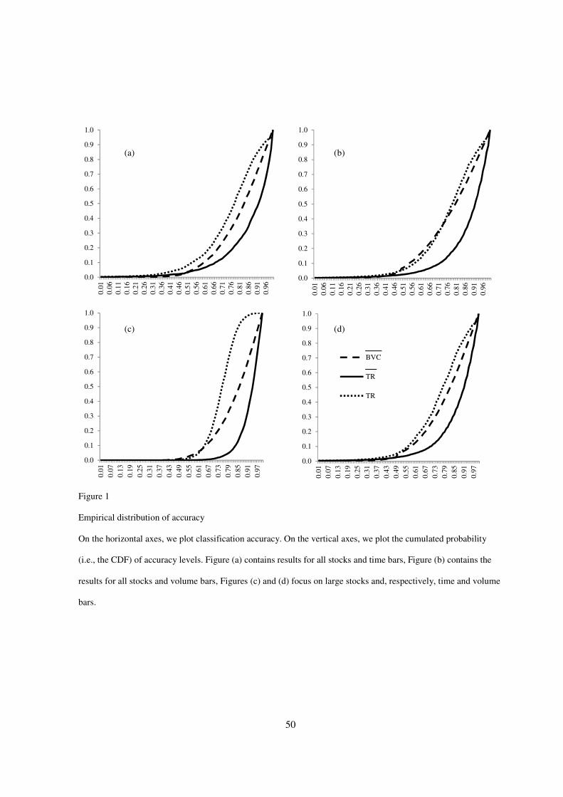
50

Figure 1

Empirical distribution of accuracy

On the horizontal axes, we plot classification accuracy. On the vertical axes, we plot the cumulated probability

(i.e., the CDF) of accuracy levels. Figure (a) contains results for all stocks and time bars, Figure (b) contains the

results for all stocks and volume bars, Figures (c) and (d) focus on large stocks and, respectively, time and volume

bars.

0.0

0.1

0.2

0.3

0.4

0.5

0.6

0.7

0.8

0.9

1.0

0.0

10.0

60.1

10.1

60.2

10.2

60.3

10.3

60.4

10.4

60.5

10.5

60.6

10.6

60.7

10.7

60.8

10.8

60.9

10.9

6

0.0

0.1

0.2

0.3

0.4

0.5

0.6

0.7

0.8

0.9

1.0

0.0

1

0.0

6

0.1

10.1

6

0.2

1

0.2

6

0.3

1

0.3

6

0.4

1

0.4

6

0.5

1

0.5

6

0.6

1

0.6

6

0.7

1

0.7

6

0.8

1

0.8

6

0.9

1

0.9

6

0.0

0.1

0.2

0.3

0.4

0.5

0.6

0.7

0.8

0.9

1.0

0.0

1

0.0

7

0.1

3

0.1

9

0.2

5

0.3

1

0.3

7

0.4

3

0.4

9

0.5

5

0.6

1

0.6

7

0.7

3

0.7

9

0.8

5

0.9

1

0.9

7

0.0

0.1

0.2

0.3

0.4

0.5

0.6

0.7

0.8

0.9

1.00.0

1

0.0

7

0.1

3

0.1

9

0.2

5

0.3

1

0.3

7

0.4

3

0.4

9

0.5

5

0.6

1

0.6

7

0.7

3

0.7

9

0.8

5

0.9

1

0.9

7

BVC

TR (with)

TR (without)

(a) (b)

(d) (c)