trade barriers and the collapse of world trade during the ...lrazzolini/gr2001.pdf · trade...

Southern Economic Journal 2001, 67(4), 848-868

Trade Barriers and the Collapse of World Trade During the

Great Depression

Jakob B. Madsen*

Using panel data estimates of export and import equations for 17 countries in the interwar period, this paper estimates the effects of increasing tariff and nontariff trade barriers on worldwide trade over the period 1929 to 1932. The estimates suggest that real world trade contracted approximately 14% because of declining income, 8% as a result of discretionary increases in tariff rates, 5% owing to deflation-induced tariff increases, and a further 6% because of the imposition of nontariff barriers. Allowing for feedback effects from trade barriers on income and prices, discretionary impositions of trade barriers contributed about the same to the trade collapse as the diminishing nominal income.

1. Introduction

The contraction in world trade during the first phase of the Great Depression stands out as the strongest adverse shock to international trade in modem history. From 1929 to 1932 world import and export volume in the industrialized nations decreased about 30%. However, it is not well understood which factors were responsible for the collapse. The factors that have been highlighted in the literature are declining demand, escalating tariff and nontariff trade

barriers, increasing bilateral trade agreements, and international exchange rate policies. The

importance attributed to each of these factors has often been controversial. Pollard (1962, p. 200) for instance argues that for Britain the "fall in total foreign trade as a proportion of home

production was a part of a secular trend, and may well not have been caused by the tariff as such." By contrast, Khan (1946, p. 246) claims that, within 12 to 18 months, UK nominal

imports of manufactures from most of Europe and the United States were reduced by something like 60% "as a result of the tariff." Similarly, Saint-Etienne (1984, p. 29) argues that "by the

mid-1930's, international trade had become, in large proportion, barter trade" as a result of the tariffs and nontariff barriers.

Empirical studies have examined the effects of trade restrictions on incomes to explain the

declining trade for individual countries. The studies of Crucini and Kahn (1996) and Irwin

(1998) find that the tariffs were influential for the U.S. imports and exports. In his study of nominal imports to the European countries, Friedman (1974) quantified the effects of trade barriers on nominal imports, and ultimately income, by means of dummies in periods of significant tariffs and nontariff barriers. He found that trade restrictions had a significant impact

* Department of Economics, University of Western Australia, Nedlands W. A. 6907, Australia. Present address: Department of Economics and Finance, Brunel University, Uxbridge, Middlesex, UB8 3PH United Kingdom.

Comments and suggestions from two anonymous referees and financial support from the Australian Research Council are gratefully acknowledged.

Received November 1999; accepted June 2000.

848

Trade Barriers and the Collapse of Trade

on trade in a few countries. However, as Friedman himself acknowledges, the weakness of this

approach is that strong and weak forms of trade barriers are restricted to impact equally on

imports in the estimates. Coupled with the small sample problems that plagued his estimates, the trade-barrier dummies were unlikely to effectively have captured the effects of trade barriers on imports, which explains substantial variations of the estimated effects of the tariffs and the nontariff barriers across countries. The study of Eichengreen and Irwin (1995) is probably the most extensive analysis of trade flows in the interwar period. Using 561 cross-sectional bilateral trade flows over three periods (1928, 1935, and 1938) they estimate a gravity model of trade

patterns. They relate the value of bilateral flows to national income, population, distance, con-

tiguity, trade and currency block indicators, and exchange rate variability, to examine the effects on trade of trade and currency blocks, and exchange rate variability. They observe a declining marginal propensity to import and export during the Depression, which they attribute to quotas and other binding trade restrictions, but do not formally test their importance.

This paper seeks to estimate the contribution of income, tariffs, and nontariff barriers on world trade during the Depression using panel data for 17 countries over the period from 1920 to 1938. The panel data approach enables the assessment of the influence on trade of nontariff barriers from estimates of import and export functions, by using as an identifying assumption that the nontariff barriers were to some degree simultaneously imposed and relaxed across the industrialized nations during the interwar period. The estimates and extensive evidence from the literature suggest that this identifying assumption is valid (section 3). In section 4 the changes in world trade in the interwar period are decomposed into income effects, tariff effects, and nontariff barrier effects. The trade effects of the tariff changes are furthermore decomposed into deflation/ inflation-induced tariff changes and discretionary tariff-induced changes. Because a significant fraction of import duties were specific (Liepmann 1938; Crucini 1994), and therefore denominated in fixed nominal values, tariff rates were automatically pushed up by declining import prices in the first years of the Depression. Overall the decomposition shows that 41% of the collapse in world trade from 1929 to 1932 was due to discretionary escalations of trade barriers, and 59% as a result of falling nominal income, assuming that the decline in prices and output were inde-

pendent of the increasing trade barriers. However, as discussed in section 5, because nominal income was influenced by trade barriers, the discretionary impositions of trade barriers had stron-

ger trade effects than suggested by these figures. Section 6 concludes the paper.

2. Tariffs and the Pattern of World Trade in the Interwar Period

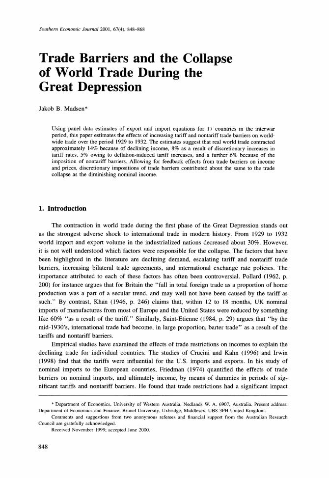
Before estimating the influence on world trade of trade barriers and income, a casual graph- ical analysis of the world macro tariff rate and the pattern of world trade is undertaken. Figure 1

displays the macro import tariff rates for the most important trading nations and the import weighted tariff rate for 22 countries in the interwar period, subsequently referred to as the world tariff rate.' The macro tariff rates are estimated as import duties divided by import value. The

figure shows that the world macro tariff rate almost doubles from 1929 to 1932, a period that was associated with the two major events in tariff policy history. The first shock was the passage

I The following 22 countries are included in the figure: Canada, the United States, Japan, Australia, New Zealand, Austria, Belgium, Denmark, Finland, France, Germany, Greece, Hungary, Ireland, Italy, the Netherlands, Norway, Portugal, Spain, Sweden, Switzerland, and the United Kingdom.

849

850 Jakob B. Madsen

0 1920 1922 1924 1926 1928 1930 1932 1934 1936 1938 1940

t

Figure 1. Macro tariff rates. Calculated as tariff duties divided by imports. The world index is computed as the USD import-weighted index for the 17 countries used in this study plus Austria, Greece, Hungary, Portugal, and Spain.

of the Hawley-Smoot Tariff Act in 1930. The second shock was the passage the Abnormal

Importation Act in November 1931 and the Import Duties Act in February 1932 by the British Parliament (Friedman 1974, p. 26). These shocks led to widespread worldwide reactions according to Jones (1934) and Friedman (1974). In his detailed taxonomy of trade barriers, Jones (1934) finds that the introduction of the Hawley-Smoot Tariff Act of 1930 led to concerted worldwide retributions against U.S. exports and escalations of trade barriers that were not specifically targeted at U.S. products. On the basis of detailed studies of major trading nations he concludes that the

Hawley-Smoot Tariff had "very definite effects upon the commercial policies of the principal trading nations of the world and upon the general development of the principles of commercial

policy throughout the world" (pp. 1-2). The Hawley-Smoot Tariff was an important catalyst for worldwide escalations of trade barriers because the United States, which was the greatest creditor nation at that time, withdrew many of its international loans and did not make new loans available, and therefore forced deficit countries to lower their imports.

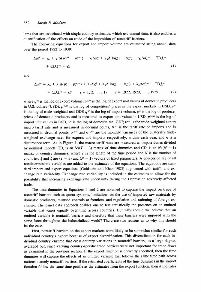
Figure 2 shows the world nominal trade flows between trade blocks and nontrade blocks in the interwar period, where the trade flows are measured by exports. The estimates are based on the 22 countries in Figure 1. The following trade/currency blocks are considered: The Sterling block, the Reichmark block, and the Gold block. This block classification follows the classification of Eichengreen and Irwin (1995), and the countries contained in each block are listed in the notes to Figure 2.2 From 1920 to 1939, 66.6% of world trade was between non-trade blocks,

2 Eichengreen and Irwin consider both currency and trade blocks. Canada, for instance, is not included in the Sterling currency block, but is a member of the Commonwealth trade block.


Index Mean=100

180 -

160-

140 -

Trade Blocks

120 -

100-

80

Non-Trade Blocks 60-

40 -

20 . . 1920 1922 1924 1926 1928 1930 1932 1934 1936 1938 1940

Figure 2. World trade among trade and nontrade blocks. The trade blocks considered are the Sterling block (Australia, New Zealand, Denmark, Finland, Ireland, Norway, Portugal, Sweden, and the United Kingdom), Reichmark block (Aus- tria, Germany, Greece, and Hungary), and Gold block (Belgium, France, the Netherlands, and Switzerland).

on average. The curves have been standardized to have a mean of 100 over the whole period. The figure shows that the gain in world trade throughout the 1920s was lost within the first four years of the Depression, when nominal world trade declined more than 50%. The two curves show significant comovements between trade and nontrade blocks, which suggests that

changes in country-specific tariffs and nontariff and trade barriers were not crucial determinants for the changes in trade flows in the interwar period. This visual impression is consistent with

Eichengreen and Irwin's (1995) results that trade between trade and currency blocks did not

gain significantly in importance, at the expense of other countries, during the Depression. Kitson and Solomou (1995) report a similar finding. It is also consistent with the evidence of Woytinsky and Woytinsky (1955, p. 80) that the distribution of international trade among continents did not change over the period 1928 to 1938. Perhaps it was realized that countries would not gain much from country-specific trade restrictions. Gardner and Kimbrough (1990) demonstrate that countries have little to gain from country-specific tariffs and that all trading partners are affected

by country-specific tariffs, not only the nations that are targeted.

3. Estimates of Imports and Exports in the Interwar Period

This section estimates import and export equations using pooled cross-section and time- series data for 17 important players in the world market during the interwar period, to disen-

tangle the effects on world trade of income, tariffs and nontariff barriers, and exchange rate

variability.3 The panel data nature of the estimates not only overcomes the small sample prob-

3 The following 17 countries, for which export and import volumes are available over the whole interwar period, are included in the estimates: Canada, the United States, Japan, Australia, New Zealand, Belgium, Denmark, Finland, France,

Germany, Ireland, Italy, Netherlands, Norway, Sweden, Switzerland, and the United Kingdom.

851

852 Jakob B. Madsen

lems that are associated with single country estimates, which use annual data, it also enables a

quantification of the effects on trade of the imposition of nontariff barriers. The following equations for export and import volume are estimated using annual data

over the period 1922 to 1939:

Aqx = Yo? + Y ,A(pdex - piex) + y2Ayi + y3A log(l + tr,x) + y4 Ar2,xr + TDt,ex

+ CDi,ex + ex (1)

and

Aqim = Xo + XA(pi - pi'im) + X2Ayd + X l( + tr log( + t X4 AOr2,m + TDt"

+ CDiim + eim i = 1, 2 ....17 t = 1922, 1923, .... 1939. (2)

where qex is the log of export volume, pd,ex is the log of export unit values of domestic producers in U.S. dollars (USD), pw.ex is the log of competitors' prices in the export markets in USD, yw is the log of trade-weighted real GDP, qim is the log of import volume, pd is the log of producer prices of domestic producers and is measured as export unit values in USD, pw"im is the log of

import unit values in USD, yd is the log of domestic real GDP, trex is the trade-weighted export macro tariff rate and is measured in decimal points, trim is the tariff rate on imports and is measured in decimal points, r2,xr' and (r2,mr are the monthly variances of the bilaterally trade-

weighted exchange rates for exports and imports respectively, within each year, and e is a disturbance term. As in Figure 1, the macro tariff rates are measured as import duties divided

by nominal imports. TD, is an Nx(T - 3) matrix of time dummies and CD, is an Nx(N - 1) matrix of country dummies, where T is the length of the time period and N is the number of countries. { and [ are (T - 3) and (N - 1) vectors of fixed parameters. A one-period lag of all nondeterministic variables are added to the estimates of the equations. The equations are standard import and export equations (Goldstein and Khan 1985) augmented with tariffs and ex-

change rate variability. Exchange rate variability is included in the estimates to allow for the

possibility that increasing exchange rate uncertainty during the Depression adversely affected trade.

The time dummies in Equations 1 and 2 are assumed to capture the impact on trade of nontariff barriers such as quota systems, limitations on the use of imported raw materials by domestic producers, misused controls at frontiers, and regulation and rationing of foreign ex-

change. The panel data approach enables one to test statistically the presence on an omitted variable that varies equally over time across countries. But why should we believe that an omitted variable is nontariff barriers and therefore that these barriers were imposed with the same force throughout the industrialized world? There are two reasons as to why this should be the case.

First, nontariff barriers on the export markets were likely to be somewhat similar for each individual country's export because of export diversification. This diversification for each individual country ensured that cross-country variations in nontariff barriers, to a large degree, averaged out, since varying country-specific trade barriers were not important for trade flows as examined in the previous section. If the export function is correctly specified, then the time dummies will capture the effects of an omitted variable that follows the same time path across

nations, namely nontariff barriers. If the estimated coefficients of the time dummies in the import function follow the same time profile as the estimates from the export function, then it indicates


that trade barrier policy was imposed and relaxed with approximately the same force and at the same time across countries.

Second, tariff rates were highly correlated over time across countries and no individual

country effects could be identified.4 If individual countries raised their tariff rates at almost the same rate and at almost at the same time, why should the timing and the force of enforcement of nontariff barriers have been any different? In fact, studies of individual countries suggest similar behavior across countries. In a detailed study of nontariff barriers, Svenska Handels- banken (1933, p. 4) found that nontariff barriers were imposed almost simultaneously across countries during the first years of the Depression. Furthermore, as discussed in the previous section, the passage of the tariff acts in the United States and United Kingdom were important catalysts for concerted worldwide retributions. This evidence is also consistent with the classification of the imposition of nontariff barriers for 12 European countries by Friedman (1974, p. 75). He finds that almost all countries had significant trade barriers between 1931 and 1935.

Similarly, in his very detailed cross-country comparison of tariffs, Liepmann (1938) notes the

similarity in timing of the imposition of import quotas for the European nations. He notes that "from about the end of year 1931, however, quotas or exchange restriction ... have become the most important instruments in commercial policy by numerous new devises such as import preventives, import monopolies for specific goods, preferential agreements, import licences, etc." (p. 41). Referring to the European countries, he further found that "not only were duties further increased between 1932 and 1935, but numerous additional restrictions were imposed on imports" (p. 357). Finally, since the decline in various real commodity prices, which com- menced in 1928 and gained momentum from 1929 to 1932, occurred almost simultaneously for all commodities, we would expect trade barriers to be imposed almost simultaneously for com-

modity exporters and therefore simultaneously affecting all countries' exports.5 It is important to note that similar magnitude and the time profile of the change in nontariff

barriers across countries is not a prerequisite for identification of the effects of nontariff barriers. It is only essential to find the average effect on world trade of the nontariff barriers, and only some similarity in timing is required for identification. Suppose that half of the countries increased their nontariff barriers in one year, whereas the other half lowered them, so that the world average remained unaltered. Then the estimated coefficient of the time dummy would be

insignificant and the estimate would correctly reveal that nontariff barriers did not influence world trade in this particular year.

The macro tariff rates in Equations 1 and 2 are separated from the price competitiveness terms because the macro tariff rates are measured ex post and hence measured as the average tariff rate after substitution effects are borne out. An escalation of the tariff on a particular item, for instance, leads to a substitution away from this item so that the macro tariff rate remains little affected by the tariff, whereas a fixed-weight tariff rate would show a significant increase. Hence, a 1% change in macro tariff rates is not likely to have the same impact on trade as a 1% change in the real exchange rate. Assuming that the average tariff rates are linear transfor- mations of the fixed-weight tariff rates, the influence of the tariff changes on trade during the

Depression can be uncovered.

4 Regressing first differences of macro tariff rates on time dummies and fixed-effect country dummies yielded highly significant estimated coefficients of the time dummies. However, all country dummies were insignificant at any conventional significance level (see also estimates of Equation 5 below). The estimates are available from the author.

5 Warren and Pearson (1937, Ch. 4) show that the path of world prices of individual commodities almost coincided with the path of an overall index of world commodity prices, particularly during the Depression.

853

854 Jakob B. Madsen

Data

Export and import volume is measured as the total weight of imports and exports. Trade-

weighted income is computed as real GDP using the average export shares to 26 different destinations over the period 1923 to 1936 as weights, which covers the period for which the most detailed international source of aggregate trade flows among countries is available, as detailed in the data Appendix. The same export weights are used in the trade-weighted export exchange rate variabilities and tariff rates on export markets. Bilateral import weights are used to compute the exchange rate variability on imports. The exchange rate variabilities are measured as the variance of trade-weighted exchange rates on a monthly basis within the year. Import competitiveness is measured as the ratio of export unit values and import unit values.

Export price competitiveness is calculated as a multilateral index. This index acknowledges the fact that exporters not only compete with producers in the market of destination, as in a

simple bilateral index, but also compete with third-market producers who export to the same market.6 For instance, German exporters selling to the Austrian market compete not only with Austrian firms but also with producers from France, Italy, Spain, and other countries that export to Austria.7 Allowing for third-country effects, export competitiveness is calculated as

pd,ex/pw,ex = pW'

where pd,ex/pw,ex is an (N X T) matrix consisting of export price competitiveness of country i at time t (i = 1, ... ., N, and t = 1, .... T), where N = 26 and T = 20. The log of the (i, t) element is therefore (pd ex -

pitex) as used in Equation 1. P is an (N X T) matrix consisting of export unit values for country i at time t denominated in USD and normalized to have a mean of one over the period 1920 to 1939. W is an (N X M) weighted matrix of N suppliers of exports to M markets:

W = {B '[(B 'cn)]' } {X[(Xcm)Cm] }

where / is the Hadamard division,8 cn is an (N X 1) vector of ones, and Cm is an (M X 1) vector of ones. The X matrix is supplier i's export market j:

XlI X12 .. XIM

- X21 X22 . .X2M

XNI XN2 ? . . XNM_

and B is the X matrix where the main diagonal matrix consists of zeros. The elements Xij are

computed as the average trade over the period 1923 to 1936. Unfortunately, data on turnover in the tradeable sector, that is, the Xii elements, are not available. Instead, Xii is measured as nominal GDP/2, which tracks the turnover of the U.S. tradeable sector in the U.S. market quite

6 A more technical note on the computation of the export competitiveness index and the data sources is available from the author.

7 The use of a multilateral index stands in contrast to previous estimates of export price elasticities in the interwar period where either bilateral indices of other ad hoc measures of price competitiveness have been used (see Orcutt 1950 for references).

8 The Hadamard division divides each element of the matrix in the numerator by each element of the matrix in the denominator.


accurately. The average nominal GDP over the period 1927 to 1936 is used, because data beyond these periods are not available for some of the 26 countries that are included in the index.

Export and import unit values are used as deflators in the competitiveness indices, mainly because they exclude the direct effects of tariffs. Other available deflators such as consumer

prices, wholesale prices, and to some extent also the value-added price deflator, can be directly misleading measures of competitiveness because they include import duties. If a country in-

creases its import duties, then its consumer and wholesale prices would increase and hence indicate a loss in its import and export price competitiveness, ceteris paribus, even if its import competitiveness has improved. Consequently, the usage of wholesale and consumer prices as deflators in a price competitiveness index would lead to severely downward-biased estimates of the price elasticities in foreign trade because of the negative correlation between the com-

petitiveness variables and the error terms. This is particularly true in the interwar period in which tariffs fluctuated substantially.

Estimation Method

Equations 1 and 2 are estimated using pooled cross-section and time-series analysis. This

approach is useful because it enables the identification of time dummies. The time dummies are not only likely to capture the effects of nontariff barriers on trade, but are also likely to enable a better identification of the income elasticities. Because income and nontariff barriers are highly negatively correlated, as shown below, omission of the time dummies is likely to lead to biased estimates of income elasticities. Furthermore, the availability of 18 annual ob- servations for each individual country, after lags and first differences are allowed for, renders

single country estimates inefficient and excessively sensitive to outliers. The equations are estimated using a generalized instrumental variable estimator, which

assumes the following covariance matrix structure (Kmenta 1986, Ch. 12):

E{e} = 2?, i= 1, 2, ..., 17, Ejt {e i, = , i $ j,

where Ei is the disturbance term for country i at time t, cr2 is its variance, and ,ij is the

contemporaneous covariance of the disturbance terms across countries. The error terms are assumed to be contemporaneously correlated across countries, as the countries have been ex-

posed to shocks that affected all countries simultaneously. Examples of such shocks were the

monetary shocks, which may have been transmitted across the world by the gold standard, the comovements of commodity prices and share prices across the world, and the volatility of the

exchange rates in the beginning of the 1920s and 1930s. The cross-country variance hetero-

geneity correction is undertaken as Bartlett tests rejected the null hypothesis of variance con-

stancy across countries, at the 1% level (see the tests in Table 1). C/2 and uoi are estimated using the feasible generalized least-squares method, which is described in Kmenta (1986, Ch. 12). Instruments are used for the price competitiveness variables. The instruments are listed in the notes to Table 1.

Estimation Results

The results of estimating the restricted versions of Equations 1 and 2 are presented in the first two columns of Table 1. The estimated coefficients of exchange rate variabilities, lagged incomes, lagged tariffs, and the lagged dependent variables were insignificant for both exports and imports, at the 5% level, and were consequently omitted from the estimates. The diagnostic

855

Table 1. Parameter Estimates of Import, Export, and Tariff Equations

Exports Imports Tariffs

AyW A(p dex - p W,ex)

Ar,-I - Ptx) Alog(1 + trlx) TD1923

TD1924

TD1925 TD1926 TD1927 TD1928 TD1929

TD1930 TD1931 TD1932 TD1933

TD1934

TD1935

TD1936

TD1937

CDjapan CDFrance

CDlreland Cons

R2(Buse) F(119,170) Chow(23, 260) DW(M) Learner BP(5) BART(16) Est. period

1.27 (25.8) -0.37 (25.0) -0.10 (10.1) -1.25 (13.2)

0.40 (0.68) 2.20 (3.66)

-0.12 (0.26) 4.58 (8.46) 3.23 (6.57) 2.76 (5.29)

-0.95 (1.92) -2.86 (5.09)

0.52 (0.78) -3.03 (4.82)

0.57 (1.15) -1.61 (3.37) -0.85 (1.81)

0.62(1.11) 3.45 (5.35) 5.64 (5.30)

-5.69 (5.52) -4.68 (4.72)

0.31 (0.77)

0.97 1.01 0.66 1.94

14.66 0.91

32.07 1922-1939

Ayd A(pd _ p w,im) A(p , - ptin) \(p d _ p w,im)

Alog(1 + tri,m) TD1923 TD1924

TD1925

TD1926

TD1927

TD1928

TD1929 TD1930 TD1931 TD1932 TD1933

TDi934

TD1935

TD1936

TD1937

R2(Buse) F(68, 221) Chow(19, 266) DW(M) Learner BP(5) BART(16) Est. period

1.09 (35.1) 0.73 (7.05) 0.21 (13.2)

-1.86 (37.1) 4.56 (12.6) 4.33 (12.8)

-0.75 (2.86) 3.95 (12.6) 1.45 (7.38) 2.28 (9.07) 1.62 (7.80)

-0.48 (3.18) 2.53 (6.50)

-8.79 (10.8) 0.97 (6.00)

-1.95 (2.38) -3.09 (1.95) -1.94 (0.38)

5.07 (14.0)

0.98 1.69 0.71 2.03

10.15 4.00

56.59 1922-1939

APt usa Aim AP t,fi

TD1923

TD1924

TD1925

TD1926

TD1927

TDl928

TD1929

TD1930 TD1931 TD1932

TD1933

TD1934

TD1935

TD1936

TD1937

R2(Buse)

Chow(19, 266) DW(M)

BP(4) BART(16) Est. period

-0.01 (5.99) -0.09 (21.2) -0.04 (8.16) -0.19 (7.31)

0.37 (1.34) -0.36 (9.25)

0.45 (0.69) 0.25 (2.84)

-0.06 (6.08) 0.30 (2.07) 0.11 (4.26)

-0.01 (5.71) 1.97 (15.6) 2.24 (17.9) 0.73 (2.23)

-0.15 (6.64) 0.09 (4.20)

-0.70 (12.1) -2.26 (25.5)

00 1.Ji

0N

0-

0.95

0.35 2.52

2.20 21.27 1922-1939

Absolute t-statistics are given in parentheses. R2 = Buse's R-squared. BART(16) = Bartlett's test for cross-country variance homogeneity, and is distributed as X2(16) under the null hypothesis of homoscedasticity. DW(M) = modified Durbin-Watson test for first-order serial correlation in fixed-effect panel data models (see Bhargava, Franzini, and Narendranathan 1982). BP(i) = fixed-effect model Breusch-

Pagan test for heteroscedasticity using the stochastic explanatory variables of the model as regressors plus a constant term, on the basis of within-individual residuals, and is distributed as x2(i) under the null

hypothesis of homoscedasticity. Chow(i, j) = F-test for coefficient constancy with breaking point in 1930/1931, and is distributed as F(i, j) under the null hypothesis of coefficient constancy. F(i, j) = F-test for cross-country coefficient constancy, and is distributed as F(i, j) under the null hypothesis of coefficient constancy. CDi = fixed-effect dummy for country i. Con = constant term. Leamer = Leamer's critical value for the F-test for coefficient constancy across countries. pi.A = percentage import price change for the following countries: Canada, New Zealand, Belgium, Denmark, Germany, Ireland, the Netherlands, Norway and Sweden. Apn," = percentage import price change for the following countries: Japan, Australia, France, Italy, Switzerland and the United Kingdom. The following instruments are used for A(p,dx _ pse~): A(pa? ), _ p?T,), Ayw , Aqet , ApcPl, Ay', Alog(l + try), Alog(l + tr?e_). The following instruments are used for A(pd -p?m): A(p, - P ?T'), AY,, Ay, , A_'pl, Alog(1 + trim), Alog(l + tri,1),

AhO, Azh0, , where hO is the log of currency in circulation. The constant terms in the import and tariff equations are excluded because the time dummies have been constant term corrected by the constant terms.


tests of the estimates in Table 1 are based on within individual ordinary least squares residuals to remove fixed country effects. The diagnostic tests do not indicate the presence of first-order serial correlation and heteroscedasticity. The null hypothesis of coefficient constancy with break-

ing point in 1930/1931 cannot be rejected at conventional significance levels, which suggests that the equations are well specified. If the time dummies are excluded from the estimates, then the null hypothesis of coefficient constancy over the two periods is rejected for both exports and imports, at the 5% level. In particular, the estimated income elasticity is substantially higher in the pre-Depression period than during the Depression when the time dummies are excluded from the estimates, which suggests that the estimated income elasticities are biased in estimates that exclude time dummies because income and nontariff barriers are contemporaneously correlated. This result highlights the importance of including the time dummies in the estimates.

The null hypothesis of cross-country coefficient constancy cannot be rejected at conventional significance levels for exports. The null hypothesis is marginally rejected at the 1% level for imports. However, the classical F-test does not take into account that the likelihood of

rejecting the null hypothesis increases with the sample size and hence that the null hypothesis of cross-country coefficient homogeneity is likely to be rejected in the large sample that is considered here. To cater for that problem, Leamer's (1978, p. 114) formula is used to calculate the critical values of diffuse priors, which takes into account that the likelihood of rejecting the null hypothesis grows with the sample size. The critical values are presented for each equation in Table 1. Because the F-statistics are well below the critical values calculated from Leamer's formula, the null hypothesis of cross-country coefficient homogeneity cannot be rejected at conventional significance levels. It follows that the coefficient estimates, which are restricted to be the same across countries, are unbiased.

The estimated income elasticities in exports and imports are slightly above one, which

gives further credit to the panel data approach where time dummies are included. Most estimated income elasticities for the interwar period in the literature are significantly below one. Friedman (1974), for instance, estimates income elasticities that are often very close to zero. If this was true, then it would imply that traded commodities are inferior goods and therefore that the ratio of world trade in total income will go towards zero in the long run. The postwar evidence

suggests that this has not been the case (see Goldstein and Khan 1985; Madsen 1998). Consistent with the finding of Eichengreen and Irwin (1995), increasing exchange uncertainty during the

Depression did not influence world trade. This finding is also consistent with findings from the

postwar period (Goldstein and Khan 1985). Changes in price competitiveness influence trade flows over a two-year time span, which

indicates that changes in relative prices take time to take full effect. The estimated price elasticities are statistically highly significant and the sum of the absolute value of long-run price elasticities of imports and exports is 1.41, which suggests that the Marshall-Lerner condition is easily satisfied. Devaluations were therefore effective tools to improve trade balances in the interwar period. The absolute estimated price elasticities are higher for imports than for exports, which is likely to reflect that export price competitiveness is measured with a larger error than the import price competitiveness or that exporters may seek alternative export markets as the real exchange rates change between export markets.9

9 The trade literature has often suggested that export price elasticities are biased toward one if export unit values are used as deflators (see Goldstein and Khan 1985). However, Madsen (1998, 1999) has shown analytically that export price elasticities are biased toward a number close to zero because of errors-in-variables.

857

858 Jakob B. Madsen

Turning to the estimates of trade barriers, the estimated tariff elasticities are approximately twice as high as the estimated long-run price elasticities and are statistically highly significant. This finding suggests that the macro tariff rates underestimate fixed-weight tariff rates by a factor of about 50%, since the trade volume effects of relative changes in tariffs and real effective exchange rates on similar commodities are the same. This result highlights the importance of separating the effects of changes in relative prices and tariffs changes on trade in estimates of export and import equations.

Turning to the estimated coefficients of the time dummies in the export and import equations, they are mostly highly significant and follow almost the same time profile for imports and exports. However, imports appear to be more adversely affected by nontariff barriers than exports during the Depression. The difference arises because the estimated income elasticity is higher for exports than for imports. Hence, less of the import decline in the first years of the Depression is explained by the fall in income.

For exports and imports on average the estimated coefficients of the time dummies show that world markets became increasingly integrated during the 1920s, which reflects catch-up to pre-World War I levels and increasing international efforts to lower trade barriers. Several con- ferences were held between 1924 and 1927 aimed at reducing quantitative restrictions and substantial progress was achieved in elimination of trade restrictions over the period from 1926 to 1928 (Woytinsky and Woytinsky 1955, p. 293; Friedman 1974, pp. 15-18).

1929 marks a turning point in the world trade expansion, induced by lower nontariff barriers. Trade volume contracts about 6% from 1930 to 1932, and declines further about 3% from 1933 to 1935/1936, as a result of increasing nontariff barriers. The years 1935 and 1936 are the darkest years in the history of trade barriers. "In 1935, every country in Europe was using almost every known method of trade restriction" (Friedman 1974, p. 31). 1937 marks a new turning point. Relaxation of nontariff barriers in this year contributes to an almost 5% increase in world trade. This time profile of nontariff barriers is consistent with the cross-country classification of Friedman (1974). Friedman (1974, Table 8) identifies periods of significant escalations of nontrade barriers in 12 European countries in the period 1924 to 1938. His evidence shows that about 90% of the 12 countries had significant nontariff barriers imposed from 1931 to 1934. They were thereafter gradually abolished and only in effect in two countries in 1937. The only inconsistency with Friedman's classification appears in 1930 for imports, where the estimates in Table 1 indicate a negative trade effect of trade barriers. However, Eichengreen (1992) documents a shortfall of foreign exchange in the wake of the commodity price collapse in 1929 that forced several countries to impose foreign exchange controls. Fur- thermore, it cannot be excluded that the 1930 discrepancy was to some extent an inventory adjustment, which is not unusual in early stages of economic downturns (Goldstein and Khan 1985). The demand decline in 1930 may have caused a stronger decline in imports than was justified by income effects because inventories were reduced in the anticipation of a lower output.

The estimates indicate that 1932 is the year of the strongest rise in nontariff barriers. This result is consistent with the historical evidence from Europe that a substantial increase in France's import barriers from 1931 to 1932 spread throughout Europe in 1932 (Friedman 1974, pp. 27-28). France placed quotas on 50 major items in 1931, and increased them to encompass 1100 items in 1932. The quotas spread to Germany, Greece, the Netherlands, Poland, Romania, and Switzerland in 1932, and exchange controls were institutionalized in 1931 and 1932 in


Germany, Hungary, Spain, Czechoslovakia, Yugoslavia, Denmark, Romania, and smaller agricultural countries.

The similarities of the time profiles of the estimated coefficients of the time dummies and the world tariff rate in Figure 1 are remarkable. The macro tariff rates increased almost 10

percentage points from 1929 to 1936 and then dropped 5 percentage points in 1937. The estimated coefficients of the time dummies show almost the same pattern, and interestingly also the same magnitude, thus giving further credibility to the hypothesis that the time dummies

capture the effects of nontariff barriers. Coupled with the taxonomies that the imposition of nontariff barriers was a worldwide phenomenon and that the restrictions were to a large degree triggered by the trade policies of the United Kingdom and the United States, it can be concluded that the estimated effects of the nontariff barriers are consistent with the nonquantitative evidence and therefore that the time dummies to a large extent have captured the effects of nontariff barriers well. It cannot, however, be ruled out that some of the trade effects of the tariffs have been captured by the time dummies because the tariffs have been measured with an error.

As a final check on the reliability of the estimates in Table 1, the actual and predicted percentage change in import and export values, Vim and Vex, for the most important players on the world market at that time are shown in Table 2. Circumflexes signify predicted values. The actual and predicted changes are remarkably similar, which suggests that the estimated models

explain changes in imports and exports very well and that country-specific effects are unim-

portant, thus reinforcing the tests above of cross-country coefficient homogeneity. Although the United States experienced the strongest decline in imports and exports from 1929 to 1932, it was the first country to recover from the 1932 low. Imports and exports continued to fall in

Germany and France until 1935. The fall in imports in these countries was especially due to an almost doubling of macro tariff rates from 1931 to 1935 (see Figure 1).

4. Decomposing the World Trade Path During the Depression

This section uses the estimates in the previous section to decompose the changes in world trade during the Depression due to changes in tariffs, nontariff trade barriers, and income, assuming that exports and imports of the 17 countries considered in this paper are representative of world trade. The change in world trade due to changes in tariffs and income are calculated from the following equations:

IMUSD Aqta = -

A6 ( A log(l + trim) (3)D)

and

Aqy = ( tAYdM ) (4)

where Aqta is the tariff-induced percentage change in world trade, Aqy is the income-induced

percentage change in world trade, IMuSD is nominal merchandise imports measured in USD for

country i, IMUSD is the sum of imports for all 17 countries in USD, > is the average estimated tariff elasticity for exports and imports, and 1( is the unweighted average of the estimated income elasticities for exports and imports. Imports are used as weights in Equations 3 and 4 because

859

Table 2. Percentage Change in Actual and Predicted Imports and Exports United States France Germany United Kingdom

V ~x Vr Vir V1," Vt V~ x Vi? VV VV A Vim vim Vi V' m

1930 -30 -17 -36 -34 -14 -18 -10 -3 -11 -12 -25 -14 -24 -14 -15 -11 1931 -46 -38 -38 -27 -34 -34 -21 -38 -23 -24 -43 -37 -38 -29 -19 -30 1932 -42 -25 -45 -48 -43 -36 -34 -17 -52 -24 -36 -39 -7 -7 -20 -13 1933 7 7 9 13 -5 15 -4 -6 -17 -10 -10 0 0 4 -3 -1 1934 2 25 13 25 0 -5 -20 -9 -20 -5 5 12 5 5 7 17 1935 8 8 21 18 -13 -4 -9 -5 0 0 -6 11 8 8 3 8 1936 6 7 16 30 0 3 19 22 7 4 1 13 1 0 11 16 1937 31 18 24 20 2 17 51 21 18 15 26 32 16 20 19 26

The growth rates in imports and exports are computed as the sum of log changes in quantities and unit values multiplied by 100.

00 (0

0

to

0 a


the export weights are almost identical. Finally, the influence on world trade of changes in nontariff barriers is the average estimated time dummies in imports and exports.

Aqt is decomposed into discretionary and deflation/inflation-induced tariff changes. Be- cause information on specific and the ad valorem tariff rates on the aggregate level is not available, the deflation/inflation-induced tariff changes are recovered from estimates of the fol-

lowing equation:

A log(l + trai) = Ko + KiA log pim + TD,ttr + CDitr + Et. (5)

The coefficients of import prices are allowed to vary across countries to capture cross-country variations in specific duties. However, this estimation method is not particularly efficient unless some restrictions are imposed on the coefficient estimates. The coefficients of import prices are therefore restricted to be the same for the country groups, in which the hypothesis of coefficient

equality cannot be rejected at the 1% level. The countries were placed into groups according to the following procedure: Equation 5 was first estimated allowing the coefficients of import prices to vary across all countries. The two lowest coefficients of import prices were then tested for equality. If the hypothesis of equality was accepted, then the coefficients were restricted to be the same; otherwise coefficient equality was tested for the two countries with the second- and the third-lowest coefficients of import prices and merged if they were the same. Thereafter whether the fourth-lowest coefficient belonged to the group was tested for, and so forth. This

testing procedure resulted in four groups with the same coefficient of import prices. The group- ing of countries is listed in the notes to Table 1.

The results of estimating the restricted version of Equation 5 using the Kmenta estimator are shown in the third column in Table 1. The diagnostic tests do not give any evidence

against the model specification. Most of the estimated coefficients of the time dummies are

very significant and follow a time profile, which is remarkably similar to the path of the estimated coefficients of the time dummies in the import and export functions. This shows that nontariff barriers and discretionary tariffs were imposed almost simultaneously, as one would expect. The estimated coefficients of the time dummies are by and large zero during the 1920s but indicate a discretionary 5 percentage point increase in the macro tariff rates over the period 1931 to 1933. The estimated coefficients of import prices vary significantly across countries. They are negligible for Canada, New Zealand, Belgium, Denmark, Germany, Ireland, the Netherlands, Norway, and Sweden, suggesting that tariffs were predominantly of the ad valorem type in these countries. The estimated coefficient is much higher for Japan, Australia, France, Italy, Switzerland, the United Kingdom, the United States, and especially Finland. Hence, the deflation over the period 1929 to 1932 had quite different effects on tariffs across countries.'0

The trade effects of the deflation/inflation-induced tariff changes is calculated from the

following equation: 17 7 IMUSD

Atp = -4 ^ iA log PtIMUSD (6)

where AqtrP is the effect of the deflation/inflation-induced tariff changes on trade.

10 The estimated sensitivities on tariffs of import price changes differ slightly from the estimates of Crucini and Kahn

(1996). However, their estimates are not strictly comparable with those in Table 1 since they use GDP deflators as

opposed to import prices, estimate over the period 1900 to 1940, and do not allow for discretionary tariff changes as

captured by the time dummies.

861

862 Jakob B. Madsen

Table 3. Decomposing Relative Changes in World Trade

1 2 3 4 5 6

Price- Actual Nontariff Induced Trade Income Barriers Tariffs Total Tariffs

Aq, Aqy (t Aqa (2 + 3 + 4) AqtaP

1923 3.0 5.0 (66.6) 2.5 (33.3) 0.0 (0.0) 7.5 (100) 0.8 1924 12.0 5.9 (52.6) 3.3 (29.5) 2.0 (17.4) 11.2 (100) 0.5 1925 6.9 5.4 (51.4) -0.4 (-3.0) 0.2 (1.9) 5.2 (100) 0.4 1926 5.0 1.8 (36.7) 4.3 (87.8) -1.2 (-24.) 4.9 (100) -0.6 1927 6.5 5.3 (92.6) 2.3 (33.8) -0.8 (-11.) 6.8 (100) -0.4 1928 1.6 2.9 (58.0) 2.5 (50.0) -0.4 (-8.2) 5.0 (100) -0.1 1929 6.1 5.0 (102.) 0.3 (6.1) -0.4 (-8.1) 4.9 (100) -0.3 1930 -5.4 -3.2 (-60.) -0.7 (-13.) -1.4 (-26.) -5.3 (100) -1.4 1931 -6.6 -6.4 (-62.) 1.5 (14.7) -5.3 (52.0) -10.2 (100) -2.1 1932 -15.5 -4.5 (-27.) -5.9 (-35.) -5.8 (-35.) -16.7 (100) -1.1 1933 2.0 2.8 (122.) 0.8 (34.8) -1.3 (-57.) 2.3 (100) -0.3 1934 1.1 5.6 (151.) -1.3 (35.1) -0.6 (16.2) 3.7 (100) 0.3 1935 2.4 5.2 (186.) -2.0 (71.4) -0.4 (14.3) 2.8 (100) 0.1 1936 5.5 6.8 (94.4) -0.7 (9.7) 1.1 (15.2) 7.2 (100) 0.6 1937 16.8 6.0 (42.3) 4.3 (30.2) 3.9 (27.4) 14.2 (100) 1.1

tot = (itm + 4ix)/2. The numbers in parentheses are percentage contributions on trade of each factor.

The decomposition of the annual percentage changes in world trade volume over the

period 1923 to 1937 is shown in Table 3. The sum of the estimated effects of changes in income and nontariff and tariff barriers are very close to the changes in actual total trade, which suggests that the estimates are quite precise. In this context it is worth noting that the

decomposition is subject to three sources of errors. First, the error that is associated with the

imposition of coefficient constancy over time and across countries. This error is not serious because the null hypothesis of cross-country coefficient homogeneity and structural stability could not be rejected at conventional significance levels, as shown in Table 1, and because

predicted and actual imports and exports were very similar, as shown in Table 2. The second source of error is the standard errors that are attached to the coefficient estimates. The low standard errors attached to the coefficient estimates, however, suggest that the confidence intervals of the coefficient estimates are quite narrow. The third source of error is measurement errors. All variables in the estimated equations are measured with errors, the magnitudes of which are not easily assessed. However, because the decomposition in Table 3 is based on

country averages, the errors attached to the variables for each country tend to average out on an aggregate level.

The results in Table 3 indicate that world trade expanded uninterrupted throughout the 1920s because of increasing income, especially, and the abolition of nontariff barriers. This

expansion, however, came to a halt in 1929. From 1929 to 1932 income and tariffs contributed both to a 13% decline in world trade and nontariff barriers to a 7% decline. The subsequent increase in world trade was driven almost entirely by the income expansions. The effects of inflation/deflation-induced tariff changes are presented in the last column in Table 3. The figures suggest that 4.6% of the decline in world trade over the period 1929 to 1932 was a result of the deflation-induced tariff increases. From this it can be concluded that 13.2% in the decline in world trade volume from 1929 to 1932 was a result of discretionary impositions of trade


barriers and that 18.7% was due to the decline in nominal income, assuming that nominal income was independent of tariffs. However, if tariffs influenced both prices and output, then it becomes difficult to maintain the 13.2-18.7% split. This issue is addressed in the next section.

Although the effects on trade of trade barriers are not shown for individual countries in this paper, it would be of interest to compare with the findings of Crucini and Kahn (1996) and Irwin (1998) for the United States. Using the estimated tariff elasticities on imports in Table 1, the increase in the U.S. macro tariff rate from 13 to 25% from 1929 to 1932 resulted in

approximately a 20% decline in import volume. Using a tariff rate that is based on fixed weights, Irwin (1998) arrives at almost the same result. The results are also consistent with the finding of Crucini and Kahn (1996). They find that the tariff escalations from 1929 to 1932 explain almost half of the decline in exports and imports using their "low tariff case," which corre-

sponds to the macro tariff rates used here. The effects on imports of changes in tariffs, income, and competitiveness for trade blocks

and residual countries are estimated in Table 4. The following blocks are considered: The

Sterling, the Reichmark, the Gold, and the residual group consisting of the United States, Canada, and Japan. Nontariff barriers are not considered because the estimates in Table 1 are worldwide averages, and may therefore equally apply to all trade blocks. The figures in the Aqim columns indicate a large cross-block discrepancy in the decline in actual import volume from 1929 to 1932. The Reichmark and the residual groups, which are dominated by Germany and the United States, experienced a pronounced decline in imports. The Reichmark block

experienced a 23% decline in imports due to tariffs, 13% due to income, and 24% due to

deteriorating price competitiveness. The corresponding figures for the residual block are 10%

(tariffs), 30% (income), and 3% (competitiveness). The Sterling and the Gold blocks experienced an income-induced decline in imports of only 5% and 11%, respectively, over the

period 1929 to 1932. Tariffs appear to play a larger role than income for the decline in imports for these countries over the period 1929 to 1935, where imports declined by 18% because of tariffs for both blocks. By comparison, the income-induced decrease in imports over the same

period was -11% (Sterling) and 7% (Gold). These figures are important because they suggest that the tariff escalations may have been motivated more by political interests than by economic distress.

To get a more visual picture of the contribution of various factors to the change in world trade during the Depression, Figure 3 displays the accumulated percentage changes in trade

owing to changes in income, tariffs, and nontariff barriers from 1929 from the estimates in Table 3. The income curve indicates that income contributed to a 13% contraction in trade from 1929 to 1932. The next curves show an additional 13% trade contraction due to tariffs and a further 5% trade contraction due to nontariff barriers from 1929 to 1932.

World trade had recovered from the depth of the Depression by reaching the 1929 level in 1937. However, trade barriers remained in place from 1932 to 1936 and they were only eased somewhat in 1937, as seen from the vertical distance between the income and the nontariff barrier curves. The increase in world trade over the period 1932 to 1937 was almost entirely driven by the income recovery. The simulations show that income growth contributed to a 26% increase and easing of trade barriers to a 7% increase in world trade over this period. Except for 1937, there was therefore not much dedication by the national governments to lower trade barriers in the post-Depression period. This suggests that once trade barriers have been imposed they tend to be in place until international efforts are made to bring them down. In fact, Figure

863

00

Table 4. Changes in Imports Due to Income and Tariffs Across Trade Blocks

Sterling Reichmark Gold Residual

Azqim AAqy q Aq q Aqm Aq Aq q Aqim AqY Aqt a Aqqq Aqim Aq Aqy A<q

Percentage Change

1930 -1.1 0.3 -1.8 4.3 -11.6 -1.7 -3.5 6.9 1.8 -1.7 3.7 6.7 -15.4 -10.0 -4.9 2.7 1931 -1.3 -6.3 -5.5 5.6 -20.6 -9.4 -9.7 8.2 -1.2 -4.2 -9.2 3.5 -12.7 -8.7 -0.7 -0.6 1932 -14.8 0.7 -8.2 -2.1 -11.3 -9.2 -9.3 9.3 -16.8 -4.8 -2.1 -1.1 -19.1 -12.0 -5.0 0.8 1933 2.0 3.9 -3.4 2.5 0.4 7.2 -2.3 -0.1 4.7 3.0 -4.6 2.1 6.5 -1.4 7.1 6.2 1934 6.3 7.2 1.5 0.2 8.7 10.3 -0.5 -5.8 -10.6 0.1 -4.4 0.1 4.6 7.6 -1.1 -3.0 1935 3.3 4.7 -0.8 -2.4 -11.9 8.6 -5.5 -12.0 -3.8 0.3 -0.8 -1.9 14.7 8.2 2.3 0.6 1936 7.6 6.0 1.4 0.0 -1.4 10.0 -1.9 -5.1 5.9 1.3 3.2 -2.8 9.5 12.2 0.7 -2.6 1937 6.7 4.3 3.8 -3.2 14.2 12.1 3.2 -7.3 27.5 5.1 6.6 -6.2 16.0 6.5 1.1 0.6

See notes to Table 2 and Figure 2. The residual group consists of the United States, Canada, and Japan. Aqc is changes in import volume due to changes in import price competitiveness.


15

10-

Income induced World Trade

-5

0

-25

"^O-30 " ~s~ ~Non-tariff barrier induced World Trade

1929 1930 1931 1932 1933 1934 1935 1936 1937

Figure 3. Simulated decomposition of accumulated changes in world trade from 1929 to 1937. See main text for expla- nation.

3 shows that world trade in 1937 would have been 13% above the 1929 level had the trade

barriers been unchanged from 1929 to 1937!

5. Trade Barriers and the Depression

The results in the previous section showed that 41% and 59% of the world trade collapse over the period 1929 to 1932 was a result of the imposition of discretionary barriers and decreasing nominal income, respectively. However, the 41-59% distribution ignores the fact that tariffs and income are not independent. Some economists argue that the U.S. tariff escalations adversely affected income, thus implying that a larger proportion of the trade collapse should be attributed to the escalations of the trade barriers than the 41%. On the other hand,

proponents of endogenous tariff policies claim that it is the other way around, namely that the rising tariffs were to a large degree endogenous responses to the increasing unemployment.

The opinions on the tariff-induced income effects span from negligible (Dombusch and Fischer 1986; Eichengreen 1989; Temin 1989; Lucas 1994) to widespread (Meltzer 1976).Il

1 Advocates of endogenous tariff policies would argue that at least some of the tariff increases were endogenous responses to increasing domestic unemployment, whereas the deflation would have alleviated the push for higher tariffs (see for instance MaGee, Brock, and Young 1989). Using OLS estimates MaGee, Brock, and Young (1989) find that 75% of the variation in the U.S. macro tariff rate over the period 1900 to 1982 can be explained by endogenous tariff variables,

namely the rate of unemployment, inflation, and terms of trade. They find that the Hawley-Smoot tariff increase was smaller than predicted by their endogenous tariff model, and therefore that the tariff increase was lower than it could have been (p. 24). Because OLS estimates do not uncover causality but only the correlation between variables, it is not clear the extent to which their estimates give support for the endogenous tariff theory. Furthermore, evidence from the interwar period suggests that the tariff escalations were a response to the problems in the distressed agricultural sector rather than the increasing unemployment (Svenska Handelsbanken 1933; Eichengreen 1989; Kindleberger 1989). However, the cause of the tariff escalations is not central to this paper, which only considers the trade effects of the

impositions of the trade barriers.

865

866 Jakob B. Madsen

According to Meltzer (1976) the Hawley-Smoot Tariff Act had devastating income effects because it inhibited the working of the price-specie-flow mechanism, thus, according to Ei- chengreen (1989), having deflationary consequences for the world economy. Conversely, Ei- chengreen (1989) argues that in the absence of retaliation, the Hawley-Smoot Tariff Act would have had stimulus effects on the U.S. economy stemming from the positive supply effects of lower real wages. By assuming sticky nominal wages Eichengreen shows in a two-country Mundell-Fleming model that idiosyncratic tariff escalations lead to a reduction in the increase in real wages because they prevented prices from decreasing as much as they would have done otherwise. The reduced growth in real wages had in turn positive supply effects. However, Eichengreen suggests that the income effects of the tariff escalations for the U.S. economy depended on the retaliations.

Recently, Archibald and Feldman (1998) have argued that the uncertainty surrounding the

legislative process leading up to the passage of the Hawley-Smoot Tariff Act and the subsequent uncertainty about the foreign reactions may have led to a higher expected variance of firms' cash flow, thus curbing investment. Their empirical results suggest a significant negative effect in 1929 but not in the later years of the downturn. Crucini and Kahn (1996) have rigorously modeled the macroeconomic effects of the Hawley-Smoot Tariff Act. On the basis of a mul- tisector dynamic equilibrium trade model they show that capital accumulation was impaired by the tariff-induced increase in prices of intermediate products. Counterfactual simulations of the model reveal that tariffs could have reduced output by as much as 2% relative to the trend between 1929 and 1932.

Turning to the price effects, the tariff escalations tended to reduce import prices (exclusive of tariffs), thus leading to deflation-induced increases in macro tariff rates. The worldwide tariff escalations, particularly on agricultural products, lowered demand for traded products. For products with inelastic supply, such as agricultural products, prices would automatically decrease in almost the same proportion as the increase in the world tariff rate. This partly explains why import and export prices declined substantially more than the value-added price deflators. Whereas the world GDP deflator decreased by 13.4%, export unit values decreased by 31.0% over the period 1929 to 1932.12 Hence, parts of the deflation-induced tariff escalations were

endogenous, which suggests that some of the deflation-induced decrease in world trade should be attributed to tariffs.

6. Summary and Conclusions

This paper is the first attempt to explicitly decompose the collapse in world trade during the Depression due to deflation-induced and discretionary tariff changes, nontariff barriers, and income. Assuming independence between nominal income and tariffs, the estimates showed that world trade contracted by 13% because of falling income, 8% because of discretionary tariff escalations, 7% because of the imposition of discretionary nontariff trade barriers, and 5% as a result of deflation-induced tariff increases, from 1929 to 1932. Assuming dependence between nominal income and trade barriers, the distinction becomes less clear-cut. The tariff escalations pushed producers of tradeables down along their relatively inelastic supply schedules and, there-

12 The figures are calculated as an unweighted average for the 22 countries, which were included in the estimates in Figure 1.

Trade Barriers and the Collapse of Trade 867

fore, to some extent explain why import prices declined by 18 percentage points more than the

GDP deflators from 1929 to 1932. Hence, part of the deflation-induced tariff escalations can be attributed to the increasing tariffs. The magnitude of the income effects of the changing tariffs

appears to be controversial. However, most researchers suggest a negative income effect in the

region of 0-2%. Allowing for these feedback effects, the contribution of the imposition of the

discretionary trade barriers was about as important as the output decline in explaining the contraction in world trade.

Appendix

Import tariff rates: Import duties divided by total imports. B. R. Mitchell. 1975. European historical statistics 1750-1975. London: Macmillan; B. R. Mitchell. 1983. International historical statistics: Americas and Australasia. London: Macmillan; and B. R. Mitchell. 1982. International historical statistics: Asia and Africa. London: Macmillan.

Currency in circulation, exports, imports, wholesale prices, and consumer prices: League of Nations. Monthly bulletin of statistics. Geneva; and Mitchell. 1975, 1982, and 1983. op cit.

Exchange rates: League of Nations. Monthly Bulletin of Statistics. Geneva; and I. Svennilson. 1954. Growth and stagnation in the European economy. Geneva: United Nations Economic Commission for Europe.

Real GDP: A. Maddison. 1995. Monitoring the world economy 1820-1992, Development Centre, OECD; and Mitchell. 1975, 1982, and 1983. op cit. except for New Zealand, where the following source has been used: S. Cjhapple. 1994. "How great was the Depression in New Zealand? Neglected estimates of interwar aggregate income," New Zealand Economic Papers 28:195-203.

Import unit values, export unit values, import volume, and export volume: Canada: F H. Leacy (editor). 1983. Historical statistics of Canada. Ottawa: Statistics Canada. United States: Department of Commerce. 1975. Historical statistics of the United States: Colonial times to 1970. Washington, DC: Bureau of the Census. Japan: K. Ohkawa, M. Shinchara, and L. Meissner. 1979. Patterns of Japanese economic development: A quantitative appraisal. New Haven: Yale University Press. Australia: W. Vamplew (editor). 1987. Australians: Historical statistics. Braodway, NSW: Fairfax, Symes, and Weldon. New Zealand: F L. R. Muriel. 1970. An economic history of New Zealand to 1939. London: Collins. Belgium: Erik Buyst. 1997. New GNP estimates for the Belgium economy during the interwar period. Review of Income and Wealth 43:357-375. Denmark: H. C. Johansen. 1985. Dansk historisk statistik 1814-1980. K0benhavn: Gyldendal. Finland: R. Hjerppe. 1989. The Finnish economy, 1860-1985. Helsinki: Bank of Finland, Government Print- ing Centre. France: A. Maddison. 1962. Growth and fluctuations in the world economy, 1870-1960," Banco Nazionale del Lavoro Quarterly Review. pp. 127-191. Germany: W. G. Hoffmann. 1965. Das wachstum der Deutschen wirtschaft seit der mitte des 19. Jahrhunderts. New York: Springer-Verlag. Ireland: League of Nations. Review of world trade. Geneva and League of Nations. Monthly bulletin of statistics. Geneva. Italy: Maddison. 1962. op cit. Netherlands: C. A. van Bochove and T. A. Huitker. 1987. Main national accounting series, 1900-1986. The Netherlands: Central Bureau of Statistics. Sweden: O. Johansson. 1967. The gross domestic product of Sweden and its composition 1861-1955. Stockholm: Almqvist and Wiksell. Switzerland: H. Ritzmann-Blickenstorfer. 1996. Historical statistics of Switzerland. Zurich: Chronos. United Kingdom: B. R. Mitchell. 1988. British historical statistics. Cambridge: Cambridge University Press. Wholesale prices and export values were used to generate export unit values and export volumes for the following years and countries: Germany (1939), France (1939), and Ireland (1938 and 1939). Export prices of exporting countries weighted by import shares are used to generate import unit values and export volume for the following years and countries: Ireland (1920-1923 and 1938-1939) and Italy (1939). The import shares from the export competitiveness-weighting matrix are used.

Export tariff rates: Tariff rates on export markets weighted by bilateral trade weights, where the weights are computed as the average export to different markets over the period 1923 to 1936, which covers the period for which detailed trade weights data are available from League of Nations. Review of world trade. The weights are based on trade flows between the following 26 countries: Canada, the United States, Japan, Australia, New Zealand, Austria, Belgium, Denmark, Finland, France, Germany, Hungary, Greece, Ireland, Italy, the Netherlands, Norway, Portugal, Spain, Sweden, Switzerland, the United Kingdom, Argentina, Czechoslovakia, China, and India.

Trade-weighted real GDP: The same weighting method that is used to compute the export tariff rates is used for the same countries plus China. Real GDP for Austria, China, Hungary, Greece, Portugal, Spain, Argentina, Czechoslo- vakia, India, and China are from the same sources as listed under real GDP above.

Exchange rate variability: Computed as the variance of monthly trade-weighted exchange rates within the year. The weights for the export tariff rates are used.

Bilateral trade: In the estimates for 22 countries over the period 1920 to 1939, Mitchell. 1975, 1982, and 1983. op cit. In the estimates for 26 countries over the period 1924 to 1936, League of Nations. Review of world trade.

868 Jakob B. Madsen

References

Archibald, Robert B., and David H. Feldman. 1998. Investment during the Great Depression: Uncertainty and the role of Smoot-Hawley Tariff. Southern Economic Journal 64:857-879.

Bhargava, A., L. Franzini, and W. Narendranathan. 1982. Serial correlation and the fixed effects model. Review of Economic Studies 49:533-49.

Crucini, Mario J. 1994. Sources of variation in real tariff rates: The United States 1900 to 1940. American Economic Review 82:346-53.

Crucini, Mario J., and James Kahn. 1996. Tariffs and aggregate economic activity: Lessons from the Great Depression. Journal of Monetary Economics 38:427-57.

Dorbusch, Rudiger, and Stanley Fischer. 1986. The open economy: Implications for monetary and fiscal policy. In The American business cycle: Continuity and change, edited by Robert J. Gordon. Chicago, IL: University of Chicago Press, pp. 459-518.

Eichengreen, Barry. 1989. The political economy of the Smoot-Hawley Tariff. Research in Economic History 12:1-43. Eichengreen, Barry. 1992. Golden fetters: The gold standard and the Great Depression, 1919-1939. Oxford: Oxford

University Press. Eichengreen, Barry, and Douglas A. Irwin. 1995. Trade blocs, currency blocks, and the reorientation of world trade in

the 1930s. Journal of International Economics 38:1-24. Friedman, Philip. 1974. The impact of trade destruction on national incomes. Gainesville: The University Presses of

Florida. Gardner, Grant W., and Kent P Kimbrough. 1990. The economics of country-specific tariffs. International Economic

Review 31:575-88. Goldstein, Morris, and Mohsin S. Khan. 1985. Income and price effects in foreign trade. In Handbook of international

economics, volume 3, edited by R. W. Jones and P. B. Kenen. Amsterdam: North Holland-Elsevier Science Pub- lishers, pp. 1041-105.

Irwin, Douglas A. 1998. The Smoot-Hawley Tariff: A quantitative assessment. Review of Economics and Statistics 80: 326-34.

Jones, Joseph M., Jr. 1934. Tariff retaliation. London: Oxford University Press. Khan, A. E. 1946. Great Britain in the world economy. London: Sir Isaac Pitman. Kindleberger, Charles P. 1989. Commercial policy between the wars. In The Cambridge economic history of Europe,

Volume VIII, edited by Peter Mathias and Sidney Pollard. Cambridge: Cambridge University Press, pp. 161-96. Kitson, Michael, and Solomos Solomou. 1995. Bilateralism in the interwar world economy. Bulletin of Economic Re-

search 47:197-219. Kmenta, Jan. 1986. Elements of econometrics. New York: Macmillan. Leamer, Edward E. 1978. Specification searches: Ad hoc inference with nonexperimental data. New York: Wiley. Liepmann, H. 1938. Tariff levels and the economic unity of Europe. Edinburgh: George Allen & Unwin. Lucas, Robert E., Jr. 1994. Review of Milton Friedman and Anna J. Schwartz's 'Monetary history of the United States,

1867-1960'. Journal of Monetary Economics 34:5-16. Madsen, Jakob B. 1998. Errors-in-variables, supply side effects in estimates of price elasticities in foreign trade. Wel-

twirtschaftlishes Archiv 134:612-37. Madsen, Jakob B. 1999. On errors in variables bias in estimates of export price elasticities. Economics Letters 63:313-9. MaGee, Stephen P., William A. Brock, and Leslie Young. 1989. Black hole tariffs and endogenous policy theory:

Political economy in general equilibrium. Cambridge: Cambridge University Press. Meltzer, Alan. 1976. Monetary and other explanations of the start of the Great Depression. Journal of Monetary Eco-

nomics 21:3-16. Orcutt, Guy. 1950. Measurement of price elasticities in international trade. Review of Economics and Statistics 32:117-32. Pollard, Sidney. 1962. The development of the British economy, 1914-50. London: E Arnold. Saint-Etienne, Christian. 1984. The Great Depression 1929-1938. California: Hoover Institution Press. Svenska Handelsbanken. 1933. The great trade war. Index VIII:2-13. Temin, Peter. 1989. Lessons from the great depression. Cambridge MA: MIT Press. Warren, George F, and Frank A. Pearson. 1937. World prices and the building industry. London: Wiley & Sons.

Woytinsky, W. S., and E. S. Woytinsky. 1955. World commerce and governments: Trends and outlook. New York: Twentieth Century Fund.

trade barriers and the collapse of world trade during the ...lrazzolini/gr2001.pdf · trade...

Documents