trade and currency weapons - parisschoolofeconomics.com€¦ · trade and currency weapons ... of...
TRANSCRIPT

Trade and currency weapons∗
Agnès Bénassy-Quéré†, Matthieu Bussière‡ and Pauline Wibaux�
May 31, 2018
First draft
Abstract
The debate on trade wars and currency wars has re-emerged since the Great recession of
2009. We study the two forms of non-cooperative policies within a single framework. First,
we compare the elasticity of trade �ows to import tari�s and to the real exchange rate, based
on product level data for 110 countries over the 1989-2013 period. We �nd that a 1 percent
depreciation of the importer's currency reduces imports by around 0.5 percent in current dol-
lar, whereas an increase in import tari�s by 1 percentage point reduces imports by around 1.4
percent. Hence the two instruments are not equivalent. Second, we build a stylized short-term
macroeconomic model where the government aims at internal and external balance. We �nd
that, in this setting, monetary policy is more stabilizing for the economy than trade policy,
except when the internal transmission channel of monetary policy is muted (at the zero-lower
bound). One implication is that, in normal times, a country will more likely react to a trade
"aggression" through monetary easing rather than through a tari� increase. The result is
reversed at the ZLB.
Keywords: tari�s, exchange rates, trade elasticities, protectionism.JEL classi�cation: F13, F14, F31, F60.
∗We would like to thank Antoine Berthou, Anne-Laure Delatte, Lionel Fontagné, Guillaume Gaulier,Sébastien Jean, Philippe Martin, Thierry Mayer, Ariel Reshef, Walter Steingress, Vincent Vicard, SoledadZignago, and the participants of the 66th AFSE Meetings, 17th RIEF Doctoral Meetings in InternationalTrade and International Finance, 34th Symposium on Money, Banking and Finance, 21st Dynamic, EconomicGrowth and International Trade conference, Banque de France, CEPII and PSE seminars, NBER workshopon Capital Flows, Currency Wars and Monetary Policy, and CESifo Area Conference on the Global Economy,for helpful comments. The views are those of the authors and do not necessarily represent those of the Banquede France or the Eurosystem.†Paris School of Economics, University Paris 1 Panthéon-Sorbonne, France.‡Banque de France.�Paris School of Economics, University Paris 1 Panthéon-Sorbonne, France, [email protected].

1 Introduction
After decades of continuous progress towards global trade integration, the issue of protecti-
onism has come back at the top of the policy agenda since the 2010s. In 2018, the US
administration decided unilaterally to raise a number of import tari�s.1 While the reasons
for such reversal are diverse and complex, they may appear as a delayed reaction to "de-
industrialization" and increased inequalities observed since the 1990s (see Evenett, 2012).
Simultaneously, acrimony about non-cooperative monetary policies have been on the rise
since the global �nancial crisis (Mantega, 2010). The G20 rule that monetary policy should
not be used for "competitive devaluation"2 was tested several times. As a matter of fact,
several researchers have shown that the zero lower bound (ZLB) increases the risk of non
cooperative policies: governments have incentives to use beggar-thy-neighbour policies such
as tari�s or currency devaluations to attract global demand at the expense of their trading
partners (Caballero et al., 2015; Eggertsson et al., 2016; Gourinchas and Rey, 2016).
When combined with an export subsidy, a tax on imports theoretically has the same
impact as a currency devaluation (see Farhi et al., 2013). In both cases, the relative price
of foreign suppliers is increased in the short term; depending on pass-through e�ects and on
trade elasticities, the volume of imports falls while the volume of exports increases. In the
longer run, the upward adjustment of domestic prices progressively o�sets these e�ects.
In practice, however, there are signi�cant di�erences between tari�s and currency changes.
In particular, tari�s are a policy variable3 while exchange rates are generally determined
on �nancial markets, even though they react to policy decisions from �scal and monetary
authorities. As a result, changes in tari�s may be considered more persistent than exchange-
rate �uctuations, thus a�ecting the decision by the exporter to o�set the induced change in
relative prices by adjusting his mark-up, and of the importer to switch with another supplier.
Additionally, import tari�s may be sector-speci�c, whereas a currency devaluation a�ects all
1This has triggered an intense policy debate, see e.g. Coeuré (2018).2See, e.g. the G20-�nance communiqué of Buenos Aires, 20 March 2018.3Grossman and Helpman (1994) and Grossman and Helpman (1995) studied the impact of lobbies pressu-
ring government to increase trade protectionism.
2

sectors simultaneously, with also larger e�ect on the cost of imported inputs.
Finally, tari�s and exchange rates also di�er in their welfare implications. While trade
wars are undeniably a negative-sum game (despite the fact that they provide revenues to
the government), monetary policies that tend to depreciate national currencies may in some
cases be bene�cial to foreign countries, particularly if the latter choose appropriate policy
responses.4 When the interest rate is at the zero lower bound, Caballero et al. (2015) argue
that a "currency war" is a zero-sum game, whereas Jeanne (2018) �nds that currency wars
have a positive impact on welfare, as opposed to the large negative impact of trade wars.5
The interplay between tari�s and exchange rates is recognized by the WTO whose Article
XV may authorize trade restrictions against a "currency manipulator", after the currency
manipulation has been con�rmed by the International Monetary Fund. In turn, Article IV of
the IMF prohibits the manipulation of exchange rates in order "to prevent e�ective balance-
of-payment adjustment or to gain unfair competitive advantage". Still, it is di�cult to prove
currency manipulation. Bergsten and Gagnon (2012) consider that the conjunction of rising
foreign-exchange reserves and a current-account surplus de�nes a currency manipulator, for
countries whose GDP per capita is above the world median. However, the IMF accepts
foreign-exchange interventions or even capital controls to mitigate a large and sudden capital
in�ow (see Ostry et al., 2010). Currency manipulation would then be declared only in the
case of prolonged under-valuation of the currency with respect to an "equilibrium" exchange
rate that needs to be calculated and agreed upon. As a matter of fact, no country has ever
been declared a "currency manipulator" by the IMF.
Still, at the national level, tari�s are often intended to be used as retaliation against
perceived undervaluation by trading partners. As a matter of fact, exchange-rate variations
have been shown to be a signi�cant determinant of protectionism. In particular, Eichengreen
and Irwin (2010) show how those countries that remained in the gold standard in the 1930s
were more prone to increasing their import tari�s.6 In the United States, Congress can impose
4See Eichengreen (2013), Blanchard (2017) and Jeanne (2018) .5This result comes from the fact that a trade war depresses global demand, whereas a currency war is
stabilizing to the extent that it is carried out through expansionary monetary policies.6For post-war evidence, see Knetter and Prusa, 2003; Bown and Crowley, 2013; Georgiadis and Gräb, 2013;
3
a rise in tari�s on a country that is found to be a "currency manipulator", although the semi-
annual report of the US Treasury on foreign-exchange policies has routinely concluded that
no major country ful�lls the criteria of currency manipulation.
Surprisingly, there is limited evidence on the compared e�ects of currency undervaluation
and tari�s on trade �ows.7 While standard trade models such as Krugman (1979) or Eaton
and Kortum, 2002 would feature similar trade elasticities with respect to tari�s and to the
exchange rate, existing studies have found the former to be much larger than the latter
(see e.g. Fitzgerald and Haller, 2014, Fontagné et al., 2017, or the meta-analysis of Head
and Mayer, 2014). However, this literature relies on �rm-level data for a particular country
(Ireland for Fitzgerald and Haller, 2014, France for Fontagné et al., 2017). We are not aware
of a systematic comparison of trade elasticities to tari�s and to the exchange rate in a more
general, multi-country framework.
As for the macroeconomic literature, it has recently studied the equivalence between
import tari�s/ export subsidies and exchange rates within a DSGE framework where the
exchange rate appreciates endogenously following an increase in import duties and export
subsidies, with Taylor-type monetary policy (see Lindé and Pescatori, 2017; Barattieri et al.,
2018; Barbiero et al., 2018; Eichengreen, 2018; following Staiger and Sykes, 2010). These
results however typically rely on similar pricing behavior and similar demand elasticities with
respect to tari�s and to the exchange rate, and on monetary policy being geared at domestic
objectives. Taylor (2016) argues that a rule-based monetary system, where each central bank
follows an inward-looking Taylor rule, will not be prone to "currency wars": In such a rule-
based world, there is no space for a currency war. Consistently, a literature has developed to
try to specify the concept of currency manipulation as a deviation from the standard, general
Bown and Crowley, 2014.7In the literature, one of the two variable is often taken into account by �xed e�ects when estimating the
impact of the other one. For instance, Berthou (2008) and Anderson et al. (2013) develop a gravity model atthe industry level which allows them to estimate the impact of the real exchange rates, but trade barriers arecontrolled through �xed e�ects. Using a di�erent methodology, de Sousa et al. (2012) derive and estimate aratio-type gravity equation at the industry level for a large number of countries, which allows them to estimatethe impact on trade of tari�s and relative prices. However, they do not estimate the impact of the exchangerate itself. Relative prices react to the exchange rate depending on pass-through e�ects, which may vary acrosssectors and countries.
4

equilibrium model.8
In this paper, we consider monetary policy as a policy instrument that may be used in a
discretionary way by the government of a country to stabilize a combination of the output gap
and the trade balance after a shock. Hence we depart from the DSGE literature by studying
a short-term equilibrium where prices are �xed and monetary policy has an external objective
on the top of the domestic one.
We �rst estimate elasticities of trade to tari�s and to the exchange rate within the same
empirical speci�cation, based on product-level (HS6) bilateral trade �ows for 110 countries
over 1989-2013. We adapt the gravity model to account for the speci�c features of the real ex-
change rate, which is neither product-level nor trully dyadic (see Head and Mayer, 2014). The
results indicate that the e�ect of tari�s is much larger than that of exchange-rate movements.
In our preferred speci�cation, a 1% depreciation of the exporter's currency is associated with
a rise in exports by 0.5% (in current dollars), whereas a 1 percentage point tari� cut in the
destination country leads to a rise in exports by 1.4%. Hence, a 1% currency devaluation is
"equivalent" to a 0.34 pp tari� cut: tari�s are 2.9 times more "powerful" than the exchange
rate. Although the estimates vary across the speci�cations, the relative impact of tari�s with
respect to the exchange rate is surprisingly stable, from 2.9 to 3.4. Hence, exchange rates and
tari�s have signi�cantly di�erent impacts on trade.
In a second step, we investigate the policy implications of our estimations within a simple
macroeconomic model adapted from Blanchard (2017). We assume that the policy-maker
of an open economy has two objectives: internal and external equilibrium.9 Faced with a
negative shock on external demand, the policy-maker will cut the home interest rate and
let the currency depreciate, or increase the tari� on imports. Hence, the two instruments
are found partly substitutes. However, if both instruments are available, they are used as
8See Cline and Williamson (2010); Bergsten and Gagnon (2012); Eichengreen (2013); Blanchard (2017).9Blanchard (2017) examines the scope of international coordination by using a two-country Mundell-
Fleming model where both domestic and foreign economies care about the deviation of output from itspotential level, and about the deviation of net exports from zero. To reach these two objectives, the twoeconomies can use either �scal or monetary policy, or combine both policies. In our model, the governmentrather uses monetary and/or trade policies to reach its internal and external objectives. Fiscal policy is con-sidered non-available, e.g. due to excess indebtedness, and the proceeds from import duties cannot be used tostimulate internal demand.
5
complements. In particular, one may be used in a pro-competitive way while the other one
will be set so as to stabilize the purchasing power of domestic households.
We show that, over the range of our estimated equivalence ratio between both instruments,
the monetary reaction to a negative demand shock is always to cut the domestic interest
rate. If both instruments are available, the monetary expansion is accompanied with a trade
policy that depends on the nature of the shock. It can be optimal to cut the tari� in order
to limit the negative impact of the currency depreciation on households' purchasing power.
However, when the internal transmission channel of monetary policy is less e�ective (at the
zero lower bound), the optimal policy mix in reaction to a negative demand shock is reversed:
it becomes optimal to increase the import tari� while letting the home currency appreciate
in order to compensate the negative impact of the tari� on consumers' purchasing power.
Hence, according to our results, the ZLB may raise the likelihood of non-cooperative policies,
but more through tari�s than through monetary policies. In normal times, a country will
react to a trade "aggression" through the monetary instrument rather than through trade
retaliation. But at the ZLB it will respond through trade retaliation. The model extension
to a two-country setting con�rms our conclusions.
The rest of the paper is organized as follows. Section 2 brie�y reviews the existing literature
on trade elasticities. Section 3 outlines our econometric methodology. Section 4 presents the
data and key stylized facts. Section 5 reports the main empirical results and a few robustness
checks. Section 6 studies the policy implications within a stylized macroeconomic model.
Section 7 concludes the paper.
2 Trade elasticities compared: the literature
The empirical literature on trade elasticities has been summarized in the meta-analysis of Head
and Mayer (2014). Strikingly, the elasticities to tari�s and to the exchange rate are generally
estimated separately. One reason is that the logarithm of the real exchange rate is colinear to
the �xed e�ects used in standard gravity equations (see Section 3), which precludes studying
the impact of the real exchange rate on trade. This identi�cation problem is sometimes
6

circumvented by substituting industry-speci�c relative prices to the real exchange rate as an
explanatory variable. For instance, de Sousa et al. (2012) use a ratio-type gravity equation
for 151 countries over 1980-1996. The ratio of exports to a speci�c country over total exports
is then regressed on the relative price and the bilateral tari�. They �nd that the e�ect of
a tari� is, on average, ten times larger than that of relative prices. The problem with such
estimation is that relative prices are not a policy variable, since they incorporate the extent of
exchange-rate pass-through that may vary across products and destination countries. Hence,
the impact of relative prices cannot be directly compared to that of tari�s.
Several papers have focused only on the exchange-rate elasticity. For instance, Leigh
et al. (2015) estimate exchange rate pass through and price elasticity of volumes for a large
set of countries at the macroeconomic level. Overall, they �nd that a 10% real e�ective
depreciation in the exporter's currency is associated with a 6.4% rise in the value of exports
(in the exporter's currency), going up to a 8.4% increase at the sector-level. Similarly, Bussière
et al. (2016) provide a set of price and income elasticities for 51 countries, using a database
of bilateral trade �ows covering about 5,000 products. In their estimation with several �xed
e�ects, a 10% depreciation of the exporter's currency increases the value of exports (again, in
the exporter's currency) by 6%. Berman et al. (2012) use French �rm-level data from 1995 to
2005 and �nd that a 10% depreciation is associated to a 6% increase in the value of exports
of the average �rm. Using a unique cross-country micro-based dataset of exporters available
for 11 European countries, Berthou and Dhyne (forthcoming) �nd that a 10% appreciation of
the real e�ective exchange rate tends to reduce the exports value in euro of the average �rm
by 5% to 8%.
In turn, Berthou and Fontagné (2016) estimate the tari� elasticity of French exports
using �rm-level data. Their estimates indicate that a 10% increase in tari� in the destination
decreases exports by 25% on average. This is consistent with Fontagné et al. (2017) who
simultaneously estimate export elasticities to the real exchange rate and to tari�s at the �rm
level for France, and �nd that a 10% appreciation of the domestic currency decreases exports
7

(expressed in the exporter's currency ) by 6% while a 10% increase in the power of the tari�10
decreases exports by almost 20%.
Here we want to rely on multi-country estimations in order to inform the currency war
versus trade war debate with appropriate quanti�cation. We use product-level bilateral data
for 110 countries and adapt the gravity model to address the identi�cation problem mentioned
above.
3 Empirical methodology
The empirical trade literature has extensively shown that bilateral trade �ows are well explai-
ned by the gravity model where exports from country i to country j depend on the economic
size of both countries (corrected for their multilateral "resistence"), on the geographic distance
between them and on a set of dummy variables such as common border, common language
or membership of a free trade area.11
The recent literature has preferred to rely on the following speci�cation where country i's
exports to country j of good k during year t, Xijkt, is explained by a series of �xed e�ects:
lnXijkt = λikt + µjkt + νij + εijkt (1)
where λikt, µjkt and νij are �xed e�ects in the dimensions indicated by the indices, and
εijkt is the residual.12
Adding the logarithm of the bilateral real exchange rate of country i against country j,
lnRERijt, and the power of the tari� imposed by country j on product k imported from
country i, ln(1 + τ)ijkt, we get:
lnXijkt = α1lnRERijt + α2ln(1 + τ)ijkt + λikt + µjkt + νij + εijkt (2)
10If τ denotes the tari� rate, the power of the tari� is ln(1 + τ). Using the power of the tari� rather thanthe tari� itself allows us to circumvent the fact that the tari� is often zero (given the large network of freetrade agreements), while still estimating an elasticity. For a small tari�, we have ln(1 + τ) = τ .
11The theoretical underpinnings of the gravity model have been proposed by Anderson (1979) and Andersonand Wincoop (2003).
12The "naive" gravity speci�cation that relies on GDPs is plagued with an omitted variable bias notablyrelated to multilateral resistance (see Baldwin (2007)).
8

The problem with Equation (2) is that the real exchange rate is colinear to the exporter-
product-time �xed e�ect (λikt) and to the importer-product-time �xed e�ect (µjkt), since it
is the di�erence between countries i and j log-price indices corrected for the bilateral nominal
exchange rate. One way to get around this identi�cation issue is to substitute an exporter-
product �xed e�ect to the usual exporter-product-time �xed e�ect, and to complement it with
a vector of controls Zit that will capture the variance in the exporter-time dimension.13 We
therefore estimate the following equation:
lnXijkt = α1lnRERijt + α2ln(1 + τ)ijkt + α3Zit + λik + µjkt + νij + εijkt (3)
The dependent variable is the logarithm of exports from country i to country j in product
k during year t, expressed in current dollar. The �rst variable of interest is the logarithm
of the bilateral real exchange rate between country i and country j in year t, de�ned such
that an increase in the real exchange rate is an appreciation of the exporter's currency. The
second variable of interest is the logarithm of the power of the tari�, de�ned as the log of one
plus the bilateral tari� imposed by importer j for product k coming from country i in year t.
The vector of exporter-time controls Zit includes the exporter's GDP in current dollar and a
crisis dummy (see data section).
Alternatively, Equation (3) is estimated while replacing the exporter-importer �xed e�ect,
νij , by a set of standard gravity controls, some of which may vary over time: free trade
agreements, single market, common currency, contiguity, common language, colonial history,
and the logarithm of the distance.14
13See Head and Mayer, 2014. We assume that trade �ows are more sensitive over time to demand-sidevariables than to supply-side ones. Hence we keep the full set of �xed e�ects on the importer side, and chooseto relax the time dimension on the exporter's �xed e�ect. We check for the robustness of this choice.
14We also tried to estimate Equation (3) with exporter-importer-product �xed e�ects. However the va-riability of the tari�s in the time dimension happened to be too limited for this estimation to be carriedout.
9

4 Data
4.1 Data sources
The dataset covers 110 countries, from advanced to developing economies,15 from 1989 to
2013, with annual data. In 2013, these countries represented 83% of world exports. We use
harmonized bilateral trade data at the detailed HS6 product level from the BACI database
(Gaulier and Zignago, 2010) where trade �ows are expressed in current dollar.16
Bilateral real exchange rates are from the IMF or computed by the US Department of
Agriculture, using IMF data. Yearly-average nominal bilateral exchange rates are corrected
for consumer prices indices.17 Gross domestic product in current dollar is taken from the
Penn World Tables. The gravity controls are from Head et al. (2010), and de Sousa (2012).
Finally, the crisis dummy is constructed based on Laeven and Valencia (2012). It refers to
banking crises, currency crises and sovereign debt crises.
There exist three types of tari�s within the World Trade Organization: Most-Favored
Nation (MFN) tari�s, Preferential Trade Agreement (PTA) tari�s and bound tari�s.18 MFN
tari�s are what countries have promised to impose on all WTO members not included in
a PTA. Both MFN and PTA tari�s can vary as long as they do not get higher than the
bound tari�,19 which is individually negociated at the WTO. In pratice, MFN tari�s are the
highest tari�s WTO members can charge one another. Here we rely on the TRAINS database
(UNCTAD), at the HS6 product level. When countries i and j are covered by a PTA, we
use the corresponding tari�s. Otherwise, we retain the MFN tari�s. In all cases, tari�s are
measured at the beginning of year t.20
15See country list in Appendix A.16Using original data from the COMTRADE database, BACI is constructed by reconciling the declarations
of the exporter and the importer, providing a complete dataset for exports, at the HS6-digit product level.17Although a currency devaluation concerns the nominal exchange rate, governments generally want to
monitor the real exchange rate, which is closer to price competitiveness. Except in high-in�ation countries,the real exchange rate closely follows the nominal one in the short term.
18See http://wits.worldbank.org/. This database does not include temporary trade barriers, such as anti-dumping duties, countrevailing duties and safeguard measures.
19The gap between the bound and applied MFN rates is called the binding overhang. It is generally greaterfor developing countries than for advanced economies.
20The database includes ad valorem-equivalents of speci�c duties and import quotas, which may vary withprices. Since speci�c duties and import quotas are mostly used in agriculture, we present robustness testswhile restricting the sample to manufacturing products.
10

Table 1: Summary statistics
Mean Within s.d. Median 1st decile 9th decile
Levels
Tari�s (%) 5.70 2.9 0 0 17.5Real exchange rate (100=2010) 103.5 15.2 100 73 136.6Variations
Real exchange rate (%) 0.9 9 0.6 -1.7 3.6Tari�s (pp) -0.27 1.8 0 -0.4 0
Notes: The real exchange rate index is based 100 in 2010. The variations in the real exchange rate are notsymetrical due to the di�erent number of occurence in the database, depending on the number of productsexchanged by the country-pair at time t.
4.2 Stylised facts
Table 1 presents some summary statistics for tari�s and real exchange rates. Over our sample,
the average tari� is of 5.70%, but the median is 0%. Extreme tari�s are rare as evidenced by
the 17.5% tari� value for the last decile. The real exchange rate is much more volatile than
tari�s: on average, the (within) standard deviation is 15.2% for the former but only 2.9% for
the latter.
Figure 1 illustrates the asymmetric evolution of tari�s (PTAs and MFNs) from 1990 to
2013. The black line represents the average tari�, which is more than halved between 1990 and
2013. The dark-grey bars represent the yearly share of tari� increases, which is calculated
as the number of tari� increases in percent of total tari� lines at the exporter-importer-
product level, weighted by the share of trade �ows that are a�ected by the tari� variation.
Tari� increases pick in 1999 but they generally remain lower than 1% of all weighted tari�
lines. Finally, the light-grey bars represent the share of tari� cuts, calculated with the same
methodology. These bars re�ect the intensi�cation of trade liberalization starting in 1996,
with a pick in 2002 and subsequent weakening along the downward trend of tari�s.21 In 2013,
62% of the available tari�s in our sample are equal to zero, versus 50% in 1990.
The downward trend in tari�s is further illustrated when looking at the non-zero variations
21Trade liberalization took place both through cuts in MFN tari�s, and through an increasing number ofregional PTAs, see Key statistics and trends in trade policy 2015, UNCTAD.
11

Figure 1: Tari�s variations
in tari�s: two third of them are decreases. The average decrease is of 4.9 percentage points.
The cuts range from -0.1 percentage point22 to -3,000 pp. Increases are less frequent than
cuts, but they are generally of larger amount: +5.6 pp. on average.
Tari� hikes are generally short lived over the period of investigation, in contrast with tari�
cuts (Figure 2): on average, an increase is o�set by half a year after, whereas a decrease is
only followed by a slight increase the year after.
Figure 2: Lifespan of tari� variations
Note: Time 0 corresponds to the year of the tari� increase or cut (compared to time -1).
22 The sample includes tari�-equivalents of quotas on agricultural products wich may arti�cially increasethe count of variations. Thus, we exclude variations of less than 0.1 percentage point.
12
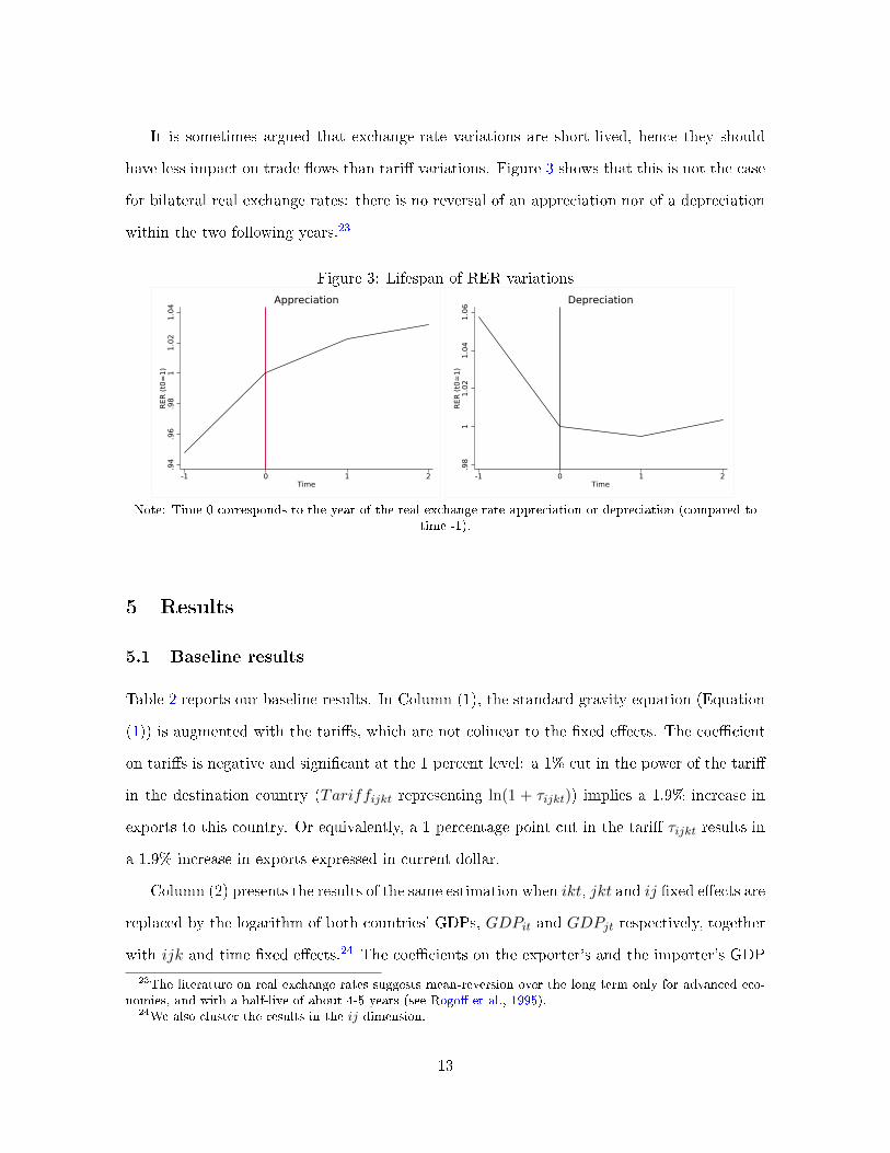
It is sometimes argued that exchange-rate variations are short-lived, hence they should
have less impact on trade �ows than tari� variations. Figure 3 shows that this is not the case
for bilateral real exchange rates: there is no reversal of an appreciation nor of a depreciation
within the two following years.23
Figure 3: Lifespan of RER variations
.94
.96
.98
11
.02
1.0
4R
ER
(t0
=1
)
-1 0 1 2Time
Appreciation
.98
11
.02
1.0
41
.06
RER
(t0
=1
)
-1 0 1 2Time
Depreciation
Note: Time 0 corresponds to the year of the real exchange rate appreciation or depreciation (compared totime -1).
5 Results
5.1 Baseline results
Table 2 reports our baseline results. In Column (1), the standard gravity equation (Equation
(1)) is augmented with the tari�s, which are not colinear to the �xed e�ects. The coe�cient
on tari�s is negative and signi�cant at the 1 percent level: a 1% cut in the power of the tari�
in the destination country (Tariffijkt representing ln(1 + τijkt)) implies a 1.9% increase in
exports to this country. Or equivalently, a 1 percentage point cut in the tari� τijkt results in
a 1.9% increase in exports expressed in current dollar.
Column (2) presents the results of the same estimation when ikt, jkt and ij �xed e�ects are
replaced by the logarithm of both countries' GDPs, GDPit and GDPjt respectively, together
with ijk and time �xed e�ects.24 The coe�cients on the exporter's and the importer's GDP
23The literature on real exchange rates suggests mean-reversion over the long term only for advanced eco-nomies, and with a half-live of about 4-5 years (see Rogo� et al., 1995).
24We also cluster the results in the ij dimension.
13

Table 2: Baseline results
Dependent variable: Exportsijkt(1) (2) (3) (4) (5) (6) (7)
Standard Simple Extended Baseline Controls Exporter's Volumegravity gravity gravity it currency
RERijt -0.300*** -0.474*** -0.472*** -0.673*** -0.269***(-8.98) (-8.02) (-7.99) (-24.04) (-6.825)
Tariffijkt -1.864*** -0.546*** -0.637*** -1.366*** -1.365*** -1.823*** -1.454***(-183.16) (-8.03) (-9.42) (-14.88) (-14.88) (-12.36) (-11.84)
GDPit 0.520*** 0.617*** 0.694*** 0.693*** 0.958***(13.17) (17.52) (12.35) (12.31) (88.28)
GDPjt 0.569*** 0.440***(25.55) (14.85)
Crisisit -0.011*(-1.86)
Real GDPit 1.107***(12.88)
FE ikt - jkt - ij Yes No No No No No NoFE ijk - t No Yes Yes No No No NoFE ik - jkt - ij No No No Yes Yes Yes YesObservations 63,746,656 63,363,339 61,611,845 63,203,049 63,203,049 59,751,140 62,409,613R-squared 0.679 0.771 0.772 0.640 0.640 0.765 0.691
Notes: standard errors are clustered at the country-pair level, t-stats are in parentheses. All variables are inlogarithm except for the in�ation; ; all nominal variables are expressed in US dollars. The level of signi�canceis the following: *** p<0.01, ** p<0.05, * p<0.1
14

are positive and highly signi�cant.25 The coe�cient on import tari�s is still negative and
signi�cant at the 1 percent level, but its size is reduced, suggesting that our two control
variables - GDPit and GDPjt - hardly capture the heterogeneity in the country-product-time
dimension.
In Column (3), we keep the same controls and �xed e�ects as in Column (2), but now add
the logarithm of the real exchange rate. The four coe�cients are signi�cant at the 1 percent
con�dence level, with the expected signs. On average, a 1% depreciation in the real exchange
rate of the exporter's country (decrease in RERijt) implies a 0.3% increase in its exports in
dollar, while a 1% cut in the power of the tari� in the destination country involves a 0.6%
increase in exports. Interestingly, the coe�cient on the power of the tari� is not signi�cantly
di�erent from the one found in Column (2).
In Column (4) the destination country's GDP is replaced by a destination-product-time
�xed e�ect in order to fully capture heterogeneity in the jkt dimension, and the other �xed
e�ects are adjusted, consistent with Equation (3). The vector of controls Zit here is limited
to the exporter's GDP, whereas Column (5) adds the crisis dummy. The residuals are still
clustered at the country-pair level. Both columns are very similar. A 1% depreciation of
the real exchange rate is associated with a 0.5% increase in exports, while a 1% cut in the
power of the tari� in the destination country is associated with a 1.4% increase in exports.
Hence, a 1% depreciation of the real exchange rate in the destination country is "equivalent",
in terms of exports, to a 0.34% tari� cut in the destination country: the tari� cut is 2.9
times more "powerful" than an exchange-rate depreciation. Since the coe�cient on the crisis
dummy is signi�cant only at the 10 percent con�dence level, we consider Column (4) as our
baseline results. Compared to Column (3), we fully account for possible omitted variables in
the destination country, although not in the origin country. The coe�cient on the tari� is
close to the one found with the standard gravity speci�cation (Column (1)), which con�rms
the adequacy of our speci�cation choice.
In Column (6), we repeat the baseline estimation while expressing the dependent variable
25Note that size and time e�ects are already captured by the �xed e�ects.
15

and the exporter's GDP in the exporter's currency rather than in US dollar.26 Both elasticities
are magni�ed compared to the baseline estimation: a 1% depreciation of the home currency
in real terms now involves a 0.7% increase in the home-currency value of exports, whereas a
1% cut in the power of the tari� in the destination country raises exports by 1.8%. Hence
a 1% depreciation is now "equivalent" to a 0.37% tari� cut: the tari� cut is 2.6 times more
"powerful" than the depreciation - a ratio not much di�erent than in the baseline estimation.
Interestingly, the elasticities found both for tari�s and for the exchange rate are close, although
slightly lower than those separately in the literature (see Section 2).27
Finally, Column (7) presents the results of the estimation in volumes, trade �ows being
de�ated by unit values. Both elasticities are smaller than in the baseline, except the estimate
on real GDP which is now equal to unity. A 1% depreciation of the real exchange rate is now
associated with a 0.27% increase in export volumes, while a 1% cut in the power of the tari�
in the destination country is associated with a 1.5% increase in export volumes. Hence, the
equivalence ratio between the two variables (5.5) is higher than for estimations run on values
but it remains around the same orders of magnitude.
Comparing Columns (6) and (7) allows us to get a quanti�cation of pricing-to-market, since
(6) is expressed in the exporter's currency whereas (7) is in volume. If a 1% appreciation in
the exporter's currency reduces its exports by 0.67% in his own currency but only by 0.27%
in volume, it must be that the export price in the exporter's currency declines by 0.67-
0.27=0.4%. Similarly, if a 1 pp increase in the destination countries' import tari� reduces
exports by 1.82% in the exporter's currency but by only 1.45% in volume, it must be that the
export price in the exporter's currency falls by 1.82-1.45=0.37%. Interestingly, the extent of
pricing-to-market is similar in both cases, implying a pass-through coe�cient of 0.6.2829
26The number of observations varies because of missing values in the nominal exchange rate used to computethe variables in the exporter's currency. We have checked however that there is no selection bias.
27By comparing elasticities estimated separately, Head and Mayer (2014) �nd trade elasticities to tari�s tobe roughly 5 times higher than trade elasticities to exchange rates. However the methodologies may not becomparable for the two average estimates. It should be reminded here that the literature generally �nds higherelasticities the more detailed the database used. Consistently, our estimation run on aggregate, bilateral trade�ows (dropping the product dimension) leads to smaller estimates for both elasticities.
28Feenstra (1989) also found symmetric pass-through for tari�s and the exchange rate on the US price ofJapanese cars, trucks and motorcycles over the 1974:1-1987:1 period.
29Our pass-through estimate is slightly lower than those found by Boz et al. (2017), while our trade elasti-
16
5.2 Robustness checks
Table 3 presents a set of robustness checks. Column (1) reproduces the baseline estimation.
In Column (2), we replace the exporter-importer �xed e�ect by a standard set of gravity
controls, some of which vary over time: common border dummy (Contiguityij), common
language dummy (Languageij), former colonial link dummy (Colonyij), geographic distance
(Distanceij), regional trade agreement (RTAijt), a common currency (Currencyijt), and
common membership to the European Union trade (EUijt). All added variables are signi�cant
at 1% with the expected sign. Using the standard errors in brackets, we see that the estimates
on the real exchange rates and on the tari� are only slightly di�erent from Columns (1).
In Column (3), we limit the sample to the pre-crisis, 1989-2007 period. The two coe�cients
of interest are not signi�cantly di�erent from baseline.
Next, we come back to the baseline speci�cation but add the �rst lag of the three variables,
in order to account for possible delayed e�ects of exchange rates and tari�s. The estimates are
reported in Column (4). The three lagged variables are highly signi�cant, with expected signs.
The coe�cient on the contemporaneous exchange rate is not much a�ected, unlike that on
the tari� which is reduced but remains signi�cant at 1%. It should be noted here that tari�s
are recorded at the beginning of the year whereas real exchange rates are yearly averages.
This di�erence may be reinforced by higher uncertainty concerning the exchange rates (which
moves every year) compared with the tari�s (which experience less frequent changes).30 31
On the whole, the elasticity of exports to the real exchange rate are found relatively stable
across the di�erent speci�cation, around 0.43-0.47 if we restrict ourselves to the estimations
carried out over the whole sample without lags. That on tari�s varies approximately from 1.3
to 1.6. We can conclude that a tari� cut in the destination country is 2.8 to 3.7 times more
cities are higher, consistent with the fact that, unlike Boz et al. (2017), we are working on product-level data.Note that we are not studying here the role of dollar invoicing because we are interested in exchange-ratepolicies vis-à-vis all other currencies.
30In an additional exercise, we tested for the impact of nominal exchange-rate volatility on trade �ows, butthe variable proved non-signi�cant.
31In an additional exercise (not shown here), we controlled for the possible colinearity between tari�s andexchange rate by orthoganalizing the tari� variable: we regressed the logarithm of one plus the tari� on thelogarithm of the real exchange rate and then introduced the residual of this equation in the baseline estimationinstead of the tari�. The results were left una�ected in sign and in magnitude.
17
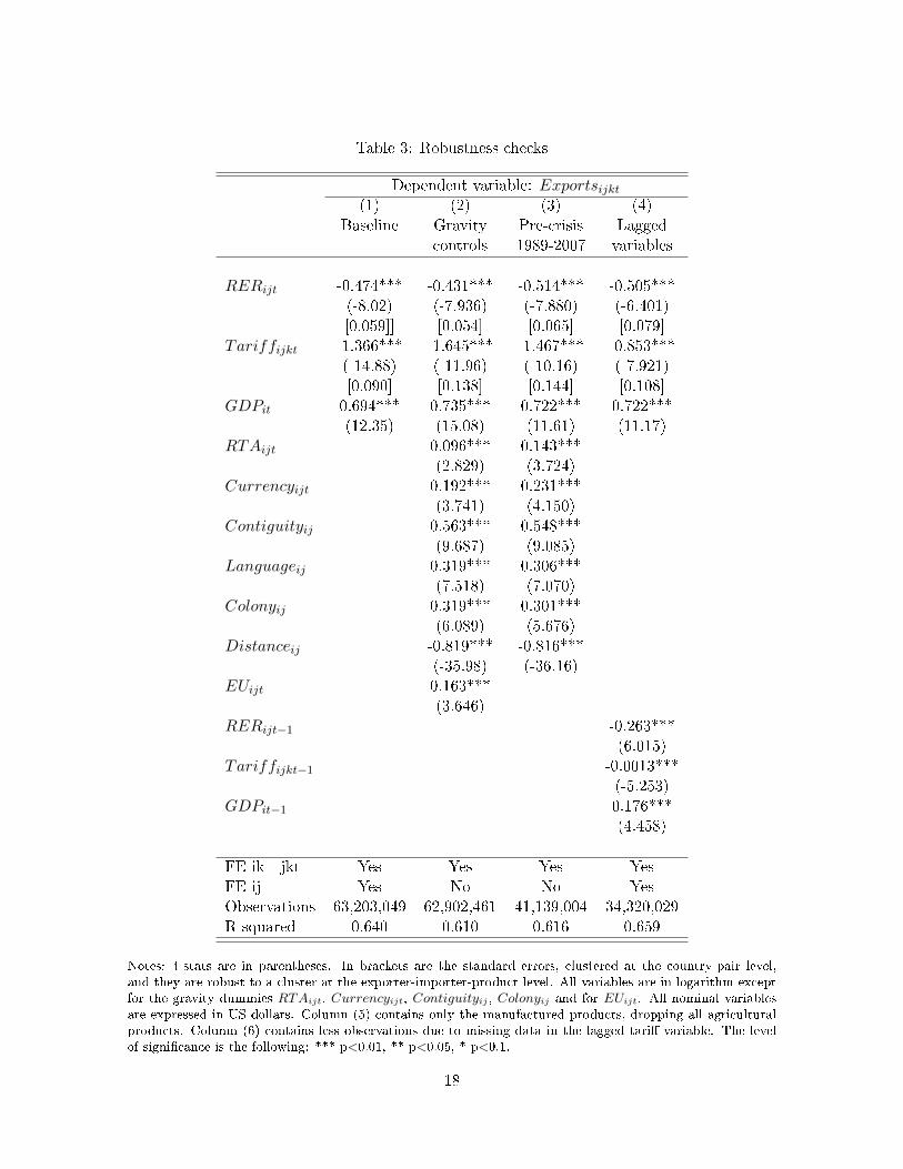
Table 3: Robustness checks
Dependent variable: Exportsijkt(1) (2) (3) (4)
Baseline Gravity Pre-crisis Laggedcontrols 1989-2007 variables
RERijt -0.474*** -0.431*** -0.514*** -0.505***(-8.02) (-7.936) (-7.880) (-6.401)[0.059]] [0.054] [0.065] [0.079]
Tariffijkt -1.366*** -1.645*** -1.467*** -0.853***(-14.88) (-11.96) (-10.16) (-7.921)[0.090] [0.138] [0.144] [0.108]
GDPit 0.694*** 0.735*** 0.722*** 0.722***(12.35) (15.08) (11.61) (11.17)
RTAijt 0.096*** 0.143***(2.829) (3.724)
Currencyijt 0.192*** 0.231***(3.741) (4.150)
Contiguityij 0.563*** 0.548***(9.687) (9.085)
Languageij 0.319*** 0.306***(7.518) (7.070)
Colonyij 0.319*** 0.301***(6.089) (5.676)
Distanceij -0.819*** -0.816***(-35.98) (-36.16)
EUijt 0.163***(3.646)
RERijt−1 -0.263***(6.015)
Tariffijkt−1 -0.0013***(-5.253)
GDPit−1 0.176***(4.458)
FE ik - jkt Yes Yes Yes YesFE ij Yes No No YesObservations 63,203,049 62,902,461 41,139,004 34,320,029R-squared 0.640 0.610 0.616 0.659
Notes: t-stats are in parentheses. In brackets are the standard errors, clustered at the country-pair level,and they are robust to a cluster at the exporter-importer-product level. All variables are in logarithm exceptfor the gravity dummies RTAijt, Currencyijt, Contiguityij , Colonyij and for EUijt. All nominal variablesare expressed in US dollars. Column (5) contains only the manufactured products, dropping all agriculturalproducts. Column (6) contains less observations due to missing data in the lagged tari� variable. The levelof signi�cance is the following: *** p<0.01, ** p<0.05, * p<0.1.
18
�powerful� than an exchange-rate depreciation in the origin country to increase the value of
bilateral exports.
5.3 Sensitivity analysis
In this section we study whether our results vary depending on the type of traded goods or
the type of exporting countries.
5.3.1 Goods
The �rst two columns of Table 4 compare the estimation results for manufactured goods and
for agricultural products, using the same speci�cation as in the baseline. Exports in manu-
factured products are more responsive to a change in the real exchange rate than agricultu-
ral products, while agricultural products are more responsive to tari�s than manufactured
products: a 1% appreciation of the exporter's currency decreases manufactured (resp. agri-
cultural) product exports by 0.48% (resp. 0.23%), while a 1% increase in the power of the
tari� decreases manufactured (resp. agricultural) exports by 1.14% (resp. 1.67%). Unsur-
prisingly given the relative sample sizes, our baseline results are closer to those obtained on
manufactured goods than to those based on agricultural goods.
We then use Rauch's classi�cation (see Rauch, 1999) to distinguish between homogenous
products (products whose prices are quoted on organized exchange or in trade publications)
and di�erentiated products. Column (3) and (4) show that the impact of both real exchange
rates and tari�s is slightly lower on di�erentiated products compared to homogenous products.
Our baseline results are close to those obtained with di�erentiated goods.
Restricting ourselves to manufactured goods, we �nd that tari�s are 2.3 times more po-
werful than exchange rates to move exports, whereas the equivalence ratio for di�erentiated
products is 3.2. In both cases, we are close to the range obtained for the whole sample (2.9
to 3.7).
19

Table 4: Trade elasticities: di�erent types of goods
Rauch classi�cation(1) (2) (3) (4)
Manuf. Agri. Homogenous Di�erentiatedproducts products products products
RERijt -0.479*** -0.230*** -0.492*** -0.459***(0.058) (0.035) (0.053) (0.0607)-7.618 -6.58 -9.28 -7.562
Tariffijkt -1.139*** -1.670*** -1.688*** -1.485***(0.166) (0.076) (0.0716) (0.195)-10.55 -21.98 -23.55 -7.609
GDPit 0.723*** 0.239*** 0.612*** 0.783***15.07 6.80 6.832 12.09
FE ik - jkt - ij Yes Yes Yes YesObservations 54,246,572 4,397,311 17,510,834 42,001,340R-squared 0.647 0.622 0.611 0.615
Notes: t-stats are in parentheses. Standard errors are clustered at the country-pair level, and they are robustto a cluster at the exporter-importer-product level. All variables are in logarithm. All nominal variables areexpressed in US dollars. The level of signi�cance is the following: *** p<0.01, ** p<0.05, * p<0.1.
5.3.2 Countries
Table 5 studies whether trade elasticities di�er for several types of countries, using the same
speci�cation as for the baseline estimations. In Column (1), we test whether the elasticity of
exports to the real exchange rate di�ers when both the exporting and the importing countries
are members of the euro area, in which case their bilateral real exchange rate only depends
on in�ation di�erentials. Speci�cally, we interact the real exchange rate with a dummy that
is equal to unity when both i and j are members of the euro area. The resulting coe�cient is
signi�cantly positive. Combining it with the non-interacted coe�cient on the real exchange
rate (which remains una�ected), we �nd that the reaction of exports to the bilateral real
exchange rate is more than halved when the two countries are part of the euro area. This
striking result does arise from membership of the single market, as evidenced by Column
(2) which interacts the real exchange rate with a dummy that is equal to unity when both i
20

and j are members of the European union, and �nds an insigni�cant coe�cient.32 Hence the
lower coe�cient found on the real exchange rate for intra-European trade is related to the
�xed nominal rate rather than to economic integration. The non-interacted coe�cient stays
una�ected, which con�rms that it can be used to study the impact of exchange rate policies
on exports.
In Column (3), we study whether trade elasticities di�er for advanced economies. Speci-
�cally, we interact the real exchange rate and the tari� with a dummy that is equal to unity
when both i and j are OECD members. The elasticity of exports to the real exchange rate is
found to be reduced for OECD countries, whereas the elasticity to tari�s is magni�ed.
Finally, Column (4) reports the results obtained when interacting tari�s and real exchange
rates with a dummy for large countries.33 It may be argued that trade between large economies
reacts more to the exchange rate or to tari�s because these countries are less likely to adjust
their margins. We �nd an insigni�cant coe�cient on the interacted dummy with the real
exchange rate, but a highly signi�cant, negative coe�cient on the interacted dummy with the
tari�. On the whole, restricting the analysis to large countries in�ates the "`equivalence"'
between tari�s and exchange rates from 2.9 in our baseline estimation to 4.2 here.
5.4 Non-linearities
As shown in Figure 2 in the data section, a tari� cut is more permanent on average than
a tari� hike. Hence a cut may have more impact on trade than a hike. This possibility is
explored in Table 6, Column (1), where the tari� is interacted with a dummy that is equal to
unity when the tari� has increased relative to the previous year. The tari� in the destination
country has signi�cantly less negative impact on exports just after an increase than when it
is either constant or declining: a 1% tari� increase in the destination country reduces exports
by 0.98%, while a 1% tari� cut stimulates exports by 1.44%. Hence, the equivalence ratio
between tari�s and the real exchange rate is 3.4 for a tari� cut but only 2.3 for a tari� increase.
32We do not repeat the same exercise for tari�s since they are equal to zero within the EU and within theeuro area.
33This country group comprises the United States, Canada, France, Germany, United Kingdom, Japan,Italy, Mexico, Turkey, South Korea and Spain.
21
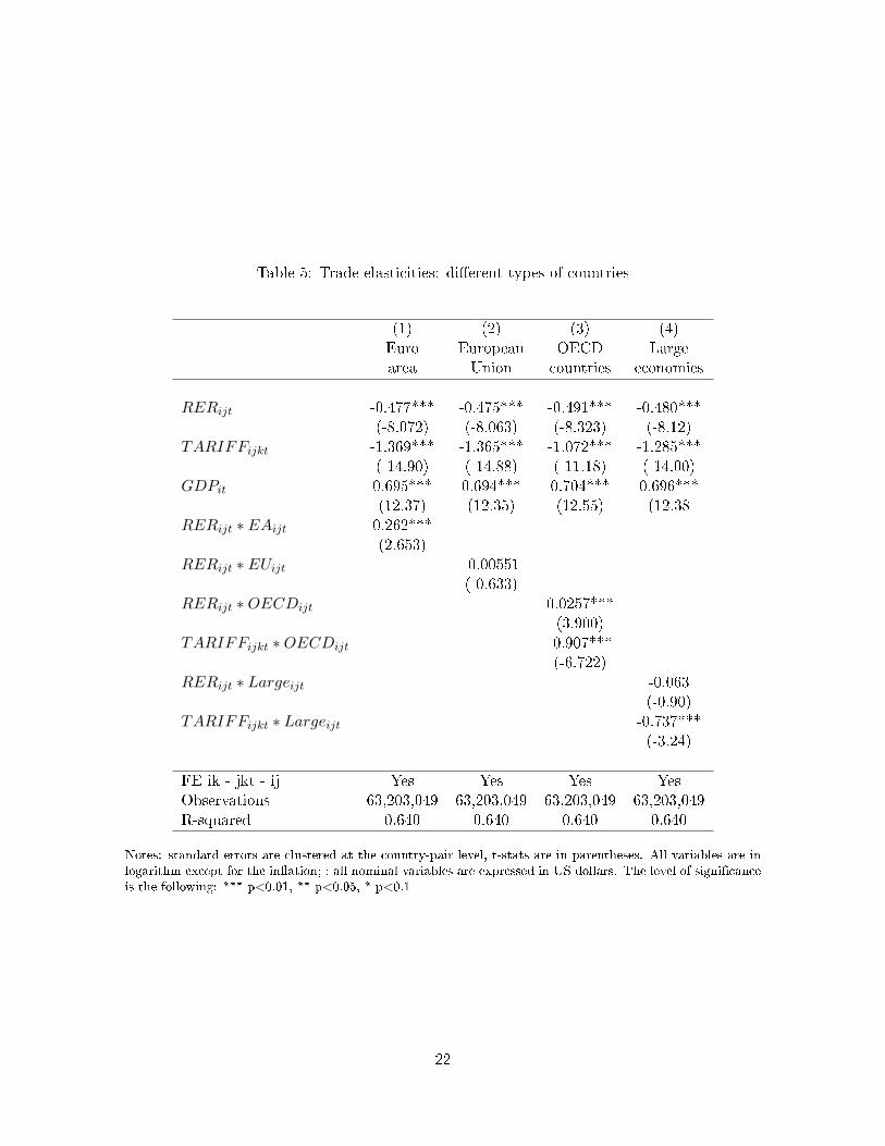
Table 5: Trade elasticities: di�erent types of countries
(1) (2) (3) (4)Euro European OECD Largearea Union countries economies
RERijt -0.477*** -0.475*** -0.491*** -0.480***(-8.072) (-8.063) (-8.323) (-8.12)
TARIFFijkt -1.369*** -1.365*** -1.072*** -1.285***(-14.90) (-14.88) (-11.18) (-14.00)
GDPit 0.695*** 0.694*** 0.704*** 0.696***(12.37) (12.35) (12.55) (12.38
RERijt ∗ EAijt 0.262***(2.653)
RERijt ∗ EUijt -0.00551(-0.633)
RERijt ∗OECDijt 0.0257***(3.900)
TARIFFijkt ∗OECDijt -0.907***(-6.722)
RERijt ∗ Largeijt -0.063(-0.90)
TARIFFijkt ∗ Largeijt -0.737***(-3.24)
FE ik - jkt - ij Yes Yes Yes YesObservations 63,203,049 63,203,049 63,203,049 63,203,049R-squared 0.640 0.640 0.640 0.640
Notes: standard errors are clustered at the country-pair level, t-stats are in parentheses. All variables are inlogarithm except for the in�ation; ; all nominal variables are expressed in US dollars. The level of signi�canceis the following: *** p<0.01, ** p<0.05, * p<0.1
22

Now, it may be argued that tari�s in the destination country have more impact on exports
when the exporter's currency is overvalued or, symmetrically, that the overvaluation of the
exporter's currency is more detrimental to exports when tari�s in the destination are high.
Column (2) shows that this is indeed the case: the coe�cient on the real exchange rate
interacted with the tari� is signi�cantly negative. Trade and monetary barriers tend to
reinforce each other.
Next, we also test whether the real exchange rate has more impact on exports when it
appreciates than when it depreciates by interacting the real exchange rate with a dummy
equal to unity when the real exchange rate has depreciated relative to the previous year.
The results reported in Column (3) show that, although signi�cant, the interacted term
bears a very small coe�cient. The almost symmetric reaction of exports to exchange-rate
appreciations or depreciations is consistent with the pattern shown in Figure 3 (contrasting
with tari�s).
Column (4) explores whether the real exchange rate has more impact on exports when
it is "misaligned", i.e. far away from its trend. For each bilateral real exchange rate, we
calculate the deviation of the log-exchange rate from a linear trend. The real exchange is
then interacted with the square of this deviation, called "misalignment". The interacted term
has signi�cant, negative e�ect on exports, con�rming that large deviations have more impact
than small ones. However the coe�cient on the (non-interacted) real exchange rate remains
close to its baseline value.34
5.5 Wrap-up
From our econometric estimations, we can draw the following conclusions: (i) as a general
rule, tari�s have around 2.9 times more impact on exports than the real exchange rate;
(ii) the equivalence ratio is slightly smaller (2.4) for manufactured goods and higher (3.2)
for di�erentiated products; (iii) it is larger (4.2) for trade between large countries; (iv) the
equivalence ratio is smaller for a tari� hike (2.3) than for a tari� cut (3.4), whereas it is
34The same exercise is not possible for tari�s due to the limited number of tari� changes at the exporter-importer-product level.
23

Table 6: Non-linear estimations
Dep. var. : Exportsijkt(1) (2) (3) (4)
RERijt -0.428*** -0.401*** -0.405*** -0.393***(-6.773) (-7.333) (-7.406) (-7.204)
Tariffijkt -1.440*** -1.743*** -1.680*** -1.677***(-11.44) (-12.68) (-12.18) (-12.18)
Tariffijkt ∗ Increase 0.461***(6.182)
RERijt ∗ Tariffijkt -0.150***(5.366)
RERijt ∗Depreciation -0.00428**(2.536)
RERijt ∗Misalignment -0.078***(3.866)
Controls Yes Yes Yes YesFE ik-jkt Yes Yes Yes YesObservations 44,222,566 63,142,608 63,142,608 63,142,608R-squared 0.630 0.609 0.609 0.609
Notes: t-stats are in parentheses. Standard errors are clustered at the country-pair level, and they are robustto a cluster at the exporter-importer-product level. All variables are in logarithm except for the gravitydummies RTAijt, Currencyijt, Contiguityij , Colonyij and for EUijt. All nominal variables are expressed inUS dollars. Column (1) contains less observations due to missing data in the tari� variable when computingits year-on-year variation. Column (4) and (5) contain less observations due to missing data in the quantityof exports variable. The level of signi�cance is the following: *** p<0.01, ** p<0.05, * p<0.1.
24
symmetric whether the real exchange rate appreciates or depreciates; and (v) the exchange
rate has more impact on trade when it is misaligned and when it interacts with relatively high
tari�s.
In the following, we set to 3 the baseline equivalence ratio between tari�s and the exchange
rate, and subsequently produce sensitivity analysis for the equivalence going from 1 to 4.
6 A stylized model of trade and currency "wars"
Here we study the implications of our estimated equivalence ratios for the reaction of a
government35 to a demand shock, based on a simple, static model adapted from Blanchard
(2017). The government is supposed to have an internal objective (GDP equal to its potential
level) and an external one (a certain level of trade balance which we set to zero for simplicity).
The relative weight of the latter objective is labelled θ.
Why could a government have an external objective on top of the stabilization of domestic
activity? First, the government may have an inter-temporal motivation: an external de�cit
today will have to be paid back tomorrow or by the next generation. This is �ne if population
and GDP are growing, but an ageing economy may aim at a trade surplus today in order to
pay for future pensions. Another reason for having an external objective is the existence of
�nancial constraints. If external debt is already high in percent of GDP, additional borrowing
may trigger a downgrading and/or an increase in interest rates. Finally, a government may
consider a trade de�cit as a progressive empoverishment of the residents and oppose the
corresponding capital in�ows (that will sometimes involve cross-border take-overs).
There may be two policy instruments (trade and monetary), in which case both objectives
can be reached simultaneously; or only one instrument (either trade or monetary), in which
case a trade-o� needs to be made between internal and external equilibrium. In our short-term
setting, an import tari� or a depreciated currency both have a positive impact on the trade
balance, but they also reduce households' purchasing power. We compare the optimal policy
35We use the term "government" in an extensive way that also incorporates the central bank. We do notdiscuss the coordination problems between the government (which decides on trade policy) and the centralbank (which decides on monetary policy).
25

(the one that minimizes the government's loss function) depending on the relative impact of
tari�s and of the exchange rate on trade �ows, and on the internal channel of monetary policy.
Then, we extend the analysis to a two country, non-cooperative setting where each government
considers the other one's policy as given. We analyse the incentive of each government to use
tari�s or monetary policy to stabilize domestic and/or foreign net demand after a negative
demand shock.
6.1 The model
We �rst consider an open economy in isolation, before moving to a two-country setting. The
starting point is the following identity:
Y = C + I +EB
P, (4)
where Y , C and I denote GDP, consumption and investment, respectively, all expressed in
units of domestic good, B is the trade balance expressed in units of foreign currency, E is the
nominal exchange rate (units of domestic currency per unit of foreign currency) and P is the
GDP de�ator.
The volume of consumption C is assumed to be a �xed share c ∈ [0, 1] of the purchasing
power of domestic income: C = cPYPc , where Pc is the consumer price index. The latter is
a weighted average of the price of domestically-produced goods P and of imported goods.
Assuming a pass-through coe�cient of π for both the exchange rate and the import tari�s
(which we have shown to be similar), the consumer price index is:
Pc = P 1−η(P ∗)η(E(1 + τ))πη, (5)
with P ∗ the price of the foreign good (in foreign currency), τ the import tari� and η ∈ [0, 1]
the share of the foreign good in the consumption basket. As for the volume of investment
I, it is assumed to react to the interest rate r with an elasticity α > 0: I0(1 + r)−α, where
I0 > 0 is a constant.
26

Since we are interested in the short-term equilibrium, we assume the price of both the
domestic and the foreign goods to be �xed: P = P ∗ = 1. Equation (4) becomes:
Y = cY [E(1 + τ)]−πη + I0(1 + r)−α + EB, (6)
The �rst term embodies the negative impact of a weaker currency (higher exchange rate
E) or an import tari� τ on aggregate demand through reduced purchasing power. The
second term shows the positive impact of a lower interest rate on aggregate demand (internal
channel of monetary policy). The third one represents net external demand. We write the
trade balance B as the di�erence between the value of exports and that of imports, both
being expressed in foreign currency. With P = P ∗ = 1, we have:
B = X0Eε(1 + τ∗)−ζεY ∗γ
∗−M0E
−ε(1 + τ)−ζεY γ (7)
where τ∗ and Y ∗ represent the foreign import tari� and foreign GDP, respectively (both
exogenous), γ, γ∗ > 0 are the home and foreign income elasticities of imports, ε > 0 is the
elasticity of exports to the exchange rate, and ζ > 0 is a multiplier applied to this elasticity
to get the elasticity of imports to the tari�. Finally, X0 > 0 and M0 > 0 are constant.
The exchange rate is assumed to be linked to the interest rate through the uncovered
interest parity, with an exogenous foreign interest rate r∗:
E =
(1 + r∗
1 + r
)δ(8)
where δ > 0 measures the expected persistence of the interest di�erential (there are no explicit
expectations in this simple, static model).
Equations (6) and (7) can be linearized around the internal and external equilibria, and
around E = 1, r = 0 and τ = 0. With y = dY/Y , y∗ = dY ∗/Y ∗, e = dE/E and b = dB/Y ,
assuming δ = 1 and denoting by u and v exogenous shocks, we get (see Appendix B):
27

y =1
1− c+ φγ
[− (2εφ−πηc+(1− c+φγ)µ)r+(φζε−πηc)τ +φ(γy∗− ζετ∗)+ v+u
], (9)
b = φ (ζε(τ − τ∗) + 2εδ(r∗ − r) + γ(y∗ − y)) + v, (10)
where µ = αI0Y (1−c+φγ) > 0 and φ = X
Y > 0.
Following Blanchard (2017), we �nally assume that the government has two objectives:
internal equilibrium (GDP equal to its potential level, e.g. a zero output gap), and external
equilibrium (a trade balance equal to zero).36 The government's programme is the following:
Mr,τinL =
1
2(y2 + θb2) (11)
The government has two policy instruments: the interest rate and the import tari�. The
interest rate has an ambiguous e�ect on domestic output: on the one hand, a rate cut sti-
mulates investment and (through the involved currency depreciation) raises net exports; on
the other hand, the depreciation reduces the purchasing power of the consumers. The tari�
also has ambiguous e�ect on output since it stimulates net exports but reduces households'
purchasing power. We expect an interest-rate cut or an increase in the import tari� to have
a positive net impact on output in the short run if the purchasing power e�ect is less than
the other e�ects.
6.2 Calibration
We calibrate our model to �t the US economy. Using the World Bank Development Indicators
for the year 2015, we recover the consumption share c = 0.7 and the ratio of trade in goods
to GDP X/Y which gives φ = 0.1. We also recover the share of the imported good in the
consumption basket, hence η = 0.2, from Hale and Hobijn (2016) .
Based on our own estimations of the elasticities of trade to the exchange rate and to the
36Alternatively, the government may target any positive or negative level of trade balance, which will nota�ect our results.
28
import tari�, we set ε = 0.5, ζ = 3, and π = 0.6. We also found an income elasticity of
exports varying between 0.45 and 0.7. We choose the median value, and set γ = 0.6. Like
Blanchard (2017), we assume δ = 1, i.e. an interest-rate variation is expected to last one year.
We calibrate µ based on the literature on the impact of a rate cut on US output (see
Appendix B). Using a DSGE model for the period from 1988 to 2013, Brayton et al. (2014)
�nd the short-term response of output to a 1 percentage point fall in the US policy rate to be
comprised between +0.1 and +0.4 percent. Focusing on the 1984-2008 period, Boivin et al.
(2010) �nd that a rate cut by 1 pp increases output by 0.2% in the short run. We select the
medium �gure of 0.3 which, given the other parameters, leads to µ = 0.3.
Finally, we assume that the internal and external objectives of the government bear equal
weights, hence θ = 1, while subsequently studying how our results react to di�erent values of
θ.
With this calibration, a 1 pp. cut in the interest rate increases the trade balance by
0.08% of GDP and output by 0.34%. Likewise, a 1 pp. increase in import tari�s increases
the trade balance by 0.14% and ouput by 0.18% despite the negative impact on purchasing
power.37 Although the tari� is more "powerful" than an exchange-rate depreciation to reduce
imports, the internal channel of monetary policy contributes to the stabilizing impact of an
interest-rate cut.
These e�ects depend on two speci�c parameters: ζ, the compared impact of the tari�
relative to the exchange rate on trade, and µ, the investment (or internal) channel of monetary
policy. The positive impact of a tari� hike on both output and the trade balance is increasing
in ζ, while the impact of monetary policy is independent from this parameter;38 in turn, a
cut in interest rate induces a larger increase in output, thus inducing a lower increase in the
trade balance when µ is large, whereas the impact of trade policy does not depend on µ.39
37The calibration gives the following partial derivatives: ∂y∂r
= −0.34, ∂y∂τ
= 0.18, ∂b∂r
= −0.08 and ∂b∂τ
= 0.14.38The partial derivatives as a function of ζ are the following (when all the other parameters are set at their
reference values): ∂y∂r
= −0.34, ∂y∂τ
= 5ζ36− 7
30, ∂b∂r
= −0.08 and ∂b∂τ
= ζ24
+ 7500
.39The partial derivatives as a function of µ are the following (when all the other parameters are set at their
reference values): ∂y∂r
= − 245− µ, ∂y
∂τ= 0.18, ∂b
∂r= 3µ
50− 73
750and ∂b
∂τ= 0.14.
29

6.3 Trade or monetary policy?
Here we simulate the reaction of the government to a negative demand shock when only one
policy instrument (trade or monetary) is available, or when both instruments are available.
Table 7 shows the optimal policy response to a negative domestic demand shock of 1
percent. When only trade policy is available (for instance, if monetary policy is constrained
by the zero lower bound, or if the country does not have an independent currency), the
government reacts by increasing the tari�, which deteriorates consumers' purchasing power,
but at the same time increases the trade balance. Ex post, output is partially stabilized.
However the trade balance increases since the higher tari� adds to the impact of lower domestic
demand to reduce imports.
With only monetary policy available (for instance, due to trade agreements or WTO
constraints), the government cuts the interest rate, which stabilizes output both through the
internal and the external channels. However this raises the trade balance. Ex post, output is
partially stabilized and the trade balance increases. The residual loss (last column of Table 7)
is smaller when the government reacts with monetary policy as when it relies on trade policy:
monetary policy is more stabilizing.
When both policy instruments are available, it is optimal to react to the domestic demand
shock by cutting the interest rate and at the same time reducing the import tari� in order to
compensate for the detrimental impact of the currency depreciation on consumers' purchasing
power. Both objectives (internal and external equilibrium) are reached since there are two
independent instruments.
The case of a negative trade shock of one percent is presented in Table 8. When there is
only one instrument available, the government responses are similar qualitatively as for the
domestic demand shock. Again, monetary policy is more stabilizing than trade policy. With
two policy instruments, though, the response is di�erent: now the government simultaneously
cuts the interest rate and raises the import tari�. Both measures weigh negatively on domestic
consumption, but this is compensated by the internal channel of monetary policy.
Our results con�rm that import tari�s and monetary policy are partly substitutes in the
30

Table 7: Policy reaction to a negative domestic demand shock u = −1%τ r b y L
One instrument: τ 0.0918 0 0.0144 -0.01069 0.0002One instrument: r 0 -0.0755 0.0077 -0.0018 0.00003Two instruments: τ , r -0.0833 -0.1250 0 0 0
Note: the table reports deviations from baseline.Source: model simulations.
Table 8: Policy reaction to a negative external shock v = −1%τ r b y L
One instrument: τ 0.1181 0 0.0081 -0.0061 0.00005One instrument: r 0 -0.0819 -0.0018 0.0004 0.000002Two instruments: τ , r 0.0200 -0.0700 0 0 0
Note: the table reports deviations from baseline.Source: model simulations.
short term, consistent with the empirical �ndings of Eichengreen and Irwin (2010) for the
interwar period. However, trade policy is clearly a second best compared to monetary policy.
When both instruments are available, they are combined di�erently depending on whether
the shock is domestic or foreign. In both cases, the government cuts the interest rate in
reaction to a negative shock. Monetary policy is accompanied by a cut in the import tari� in
case of a domestic shock, but a rise in case of a foreign shock.
Figure 4 in Appendix C plots the optimal reaction of the tari� to a negative demand shock
depending on the equivalence ratio, ζ, when only trade policy is available. For ζ higher than
about 1.5, the optimal response is an increase in the tari�, with relatively stable results from
2.9 (our baseline estimate) to 4 (for trade between large economies). However, for ζ < 1.5, it
is optimal for the government to lower the tari� since the impact of a higher tari� on output
becomes negative: the positive impact through higher net exports is less than the negative
impact through reduced purchasing power.
We now turn to the role played by the internal channel of monetary policy, represented by
µ. In Figure 5 (Appendix C), we plot the optimal monetary response to a negative demand
shock depending on this parameter. For µ = 0 to 0.4, the optimal reaction to a negative
shock is always a cut in the interest rate, although with di�erent magnitudes.
31
This �rst group of results suggests that, with our calibration, the optimal reaction to a
negative demand shock is to lower the interest rate (and depreciate the currency), whether
or not trade policy is available. Reacting to the shock through increasing the import tari� is
less stabilizing for output. If ζ is much smaller than in our calibration, it becomes optimal
to react to a negative demand shock by lowering rather than increasing the tari�. Based
on these results, it seems that there is more scope for a "currency war" than for a "trade
war". However it is mostly a question of instrument availability: when monetary policy is
constrained, trade policy can act as an imperfect substitute, and vice-versa.
6.4 Policy mix
Tables 7 and 8 show that, when both trade and monetary policy are available, the government
will react to a negative demand shock by lowering the interest rate and increasing or decreasing
the import tari� (depending on the nature of the shock). Table 9 explores the robustness of
these result with respect to the equivalence ratio ζ. It turns out that whatever ζ, the combined
reaction of monetary and trade policy is qualitatively the same. A higher ζ just implies a
lower reaction of both instruments, since trade policy becomes more powerful.
Table 10 looks at the optimal policy-mix for di�erent values of µ. For µ > 0, the optimal
response to a negative demand shock is always a cut in the interest rate, in combination with
a cut in the import tari� (domestic shock) or of either an increase or a cut in the import tari�
(external shock). The higher the internal channel of monetary policy (µ), the more limited the
cut in the interest rate (since a smaller cut becomes su�cient to stabilize aggregate demand),
but the more likely the government will increase the import tari�.
Conversely, if µ = 0, the internal channel of monetary policy is muted, so it is no longer
optimal to cut the interest rate. The stabilization of the economy then goes through an
increase in the import tari� and, simultaneously, an increase in the interest rate (and an
apreciation of the currency) to compensate the negative impact of the tari� on domestic
consumption. Interestingly, the government's response is similar for both types of shocks.
We conclude that, when both instruments are available, the reaction to a negative demand
32
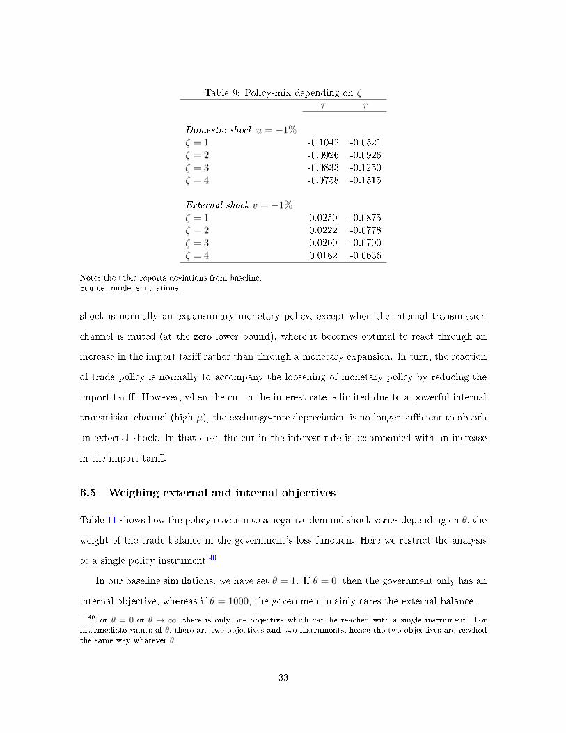
Table 9: Policy-mix depending on ζτ r
Domestic shock u = −1%ζ = 1 -0.1042 -0.0521ζ = 2 -0.0926 -0.0926ζ = 3 -0.0833 -0.1250ζ = 4 -0.0758 -0.1515
External shock v = −1%ζ = 1 0.0250 -0.0875ζ = 2 0.0222 -0.0778ζ = 3 0.0200 -0.0700ζ = 4 0.0182 -0.0636
Note: the table reports deviations from baseline.Source: model simulations.
shock is normally an expansionary monetary policy, except when the internal transmission
channel is muted (at the zero lower bound), where it becomes optimal to react through an
increase in the import tari� rather than through a monetary expansion. In turn, the reaction
of trade policy is normally to accompany the loosening of monetary policy by reducing the
import tari�. However, when the cut in the interest rate is limited due to a powerful internal
transmision channel (high µ), the exchange-rate depreciation is no longer su�cient to absorb
an external shock. In that case, the cut in the interest rate is accompanied with an increase
in the import tari�.
6.5 Weighing external and internal objectives
Table 11 shows how the policy reaction to a negative demand shock varies depending on θ, the
weight of the trade balance in the government's loss function. Here we restrict the analysis
to a single policy instrument.40
In our baseline simulations, we have set θ = 1. If θ = 0, then the government only has an
internal objective, whereas if θ = 1000, the government mainly cares the external balance.
40For θ = 0 or θ → ∞, there is only one objective which can be reached with a single instrument. Forintermediate values of θ, there are two objectives and two instruments, hence the two objectives are reachedthe same way whatever θ.
33

Table 10: Policy-mix depending on µτ r
Domestic shock u = −1%µ = 0 0.2381 0.3571µ = 0.1 -0.8333 -1.2500µ = 0.2 -0.1515 -0.2273µ = 0.3 -0.0833 -0.1250µ = 0.4 -0.0575 -0.0862
External shock v = −1%µ = 0 0.2000 0.2000µ = 0.1 -0.4000 -0.7000µ = 0.2 -0.0182 -0.1273µ = 0.3 0.0200 -0.0700µ = 0.4 0.0345 -0.0483
Note: the table reports deviations from baseline.Source: model simulations.
We �rst consider a negative shock to domestic demand. Remember that such shock
reduces domestic output but increases the trade balance, and that cutting the interest rate
leads the trade balance to increase even further. If θ is small, the government disregards
the impact of the shock and of the policy response on the trade balance, which leads to a
strong reaction through either monetary easing or a tari� hike. Conversely, if θ = 1000, the
government disregards the output gap. What is important is to stabilize the trade balance,
through an increase in the interest rate (and an exchange-rate appreciation) or through a cut
in the import tari�.
Following a negative external demand shock, both the output gap and the trade balance
decline, and a cut in the interest rate or an increase in the import tari� are stabilizing for
both variables. Hence, whatever the value of θ, it is always optimal to increase the tari� or
cut the interest rate. A greater weight on the trade balance will induce more rate cut and less
tari� hike. This is because the interest rate is relatively less powerful than the import tari�
to stabilize the trade balance, and relatively more powerful to stabilize the output gap.
This �nal set of results suggests that beggar-thy-neighbor policies are almost always op-
timal after a negative demand shock. The only exception is for a government seeking to
34

Table 11: Policy reaction to a negative demand shock, depending on θ (one instrument)τ r
Domestic shock u = −1%θ = 0 0.1515 -0.0806θ = 1 0.0918 -0.0755θ = 10 0.0122 -0.0454θ = 100 -0.0092 0.0049θ = 1000 -0.0117 0.0191
External shock v = −1%θ = 0 0.1515 -0.0806θ = 1 0.1181 -0.0819θ = 10 0.0735 -0.0891θ = 100 0.0615 -0.1012θ = 1000 0.0601 -0.1046
Note: the table reports deviations from baseline.Source: model simulations.
stabilize the trade balance after a domestic demand shock, in which case a depreciation or a
tari� hike will not help.
6.6 A two-country extension
We now come back to our baseline calibration and turn to a two-country model where Home
and Foreign are symmetric economies. We consider a non-cooperative setting where each
government tries to stabilize national output and the trade balance. They both react to a
common shock using either the interest rate or the import tari�, considering the policy of
the other government as given (Nash equilibrium). When both countries have two instru-
ments available, the model is overidenti�ed;41 therefore we only consider the cases where one
instrument is available in each country.
Although foreign policy instruments are considered exogenous to the home government,
the foreign economy itself (represented by y∗ and b∗) is not: when cutting the home interest
rate, the home government knows that doing so will a�ect foreign output, which will in turn
41Stabilizing the trade balance of the home country automatically stabilizes the trade balance of the foreigneconomy.
35

Table 12: Nash equilibria: negative demand shockτ , τ∗ r, r∗ b, b∗ y, y∗ L, L∗
Domestic shock u = u∗ = −1%One instrument: τ , τ∗ -0.1190 0 0 0 0One instrument: r, r∗ 0 -0.0926 0 0 0
External shock v = v∗ = −1%One instrument: τ , τ∗ -0.1554 0 -0.01 0.0102 0.0001One instrument: r, r∗ 0 -0.0990 -0.01 0.0023 0.00005
Note: the table reports deviations from baseline.Source: model simulations.
a�ect home exports. Thus, an additional, indirect channel of policy transmission is now at
play.
Suppose for instance that the home government cuts the home interest rate. This de-
cision will have a positive impact on home output and on the home trade balance through
the combination of the domestic transmission channel (higher investment) and the external
channel (currency depreciation increasing competitiveness but reducing purchasing power).
Now, there is also an indirect channel that goes through foreign output. Since the foreign
currency appreciates but the foreign interest rate does not increase (Nash hypothesis), foreign
output is in fact expected to increase following the shock, thanks to higher purchasing power.
Hence, the home government expects its interest-rate cut to have more positive impact on
home exports and output, compared to the small open economy case.
In turn, if the home government increases its import tari�, it can expect a fall in foreign
output, hence reduced impact on home exports and output. As shown in Table 12, it is
now optimal to react to a negative demand shock by cutting the import tari� rather than
increasing it: the tari� cut stimulates home purchasing power with little impact through the
combined direct and indirect external channels.42
Because the demand shock is symmetric and hits two symmetric economies, the reactions
are the same. A common negative demand shock (u = u∗ = −1%) decreases both outputs
but leaves the trade balances una�ected. Both government can thus stabilize their output
42In the two country setting, we have the following partial derivatives for the Home economy: ∂y∂r
= −0.21,∂y∂τ
= −0.04, ∂b∂r
= −0.1 and ∂b∂τ
= 0.15.
36
by either cutting the tari� (to regain purchasing power) or by decreasing the interest rate to
boost investment. Whatever the instrument, output is fully stabilized in both countries (see
Table 12).
When facing a negative trade shock (v = v∗ = −1%), the trade balances cannot be
stabilized, because the symmetric reactions in tari� or interest rate cancel each other. Both
countries choose to decrease the tari� or the interest rate to try to stabilize their output, just
as for a negative shock on domestic demand. Comparing the losses in the last column of Table
12 suggests that a monetary response is much more stabilizing than a trade policy.
Hence, the results obtained in the small-economy case are con�rmed in the two-country
model: with our calibration, monetary policy appears more appropriate than trade policy to
stabilize the economy after a demand shock. The risk of a trade war is now also limited by
the fact that each country anticipates the negative impact of a tari� on its own exports, even
without anticipating any form of trade retaliation.
7 Conclusion
Recent decades have witnessed a proliferation of bilateral and regional trade agreements on the
top of more and more countries being part of the World Trade Organization. This evolution
has constrained the protectionist response to shocks: unlike during the Great depression
of 1929, the Great recession of 2009 has generally not been accompanied with a revival of
protectionism, although some tari� hikes have been observed. International disputes have
then moved to the monetary sphere, with some countries being accused of leading a "currency
war".
In this paper, we compare the elasticity of exports to tari�s and to the exchange rate,
based on a panel of HS6-level bilateral trade �ows for 110 countries over 1989-2013. For the
whole sample, we �nd that a 1 percent depreciation of the exporter country's currency has
the same impact as a cut in the importer's tari� by 0.34%: a tari� cut in the destination
country is 2.9 times more "powerful" than an exchange-rate depreciation in the origin country
to increase the value of exports. This order of magnitude is shown to be relatively robust,
37

although we evidence some sensitivity depending on the types of products and of countries,
and a few non-linearities.
We then incorporate our baseline result into a simple open economy model where policy-
makers target both internal and external balance. We �nd that, if both trade and monetary
"weapons" are available, the government reacts to a negative demand shock by cutting the
home interest rate (and letting the home currency depreciate) while the accompanying trade
policy depends on the nature of the shock and on the intensity of the internal transmision
channel of monetary policy. If only one policy instrument is available, the government may
either cut the interest rate or increase the import tari�. However, increasing the import tari�
is less e�ective in stabilizing output, and in a two-country setting it is optimal to rather cut
the import tari�. One implication of our results is that, in normal times the home country
will more likely react to a trade aggression through monetary easing rather than through
retaliating on trade policy. At the ZLB, though it can be optimal to react to a trade (or
monetary) "aggression" through trade retaliation.
Our results con�rm previous research showing that the incentive to carry out non-cooperative
policies increases at the zero lower bound, when the internal transmission channel of mone-
tary policy is muted. However, we show that such non-cooperative policy is more likely to
go through a trade policy rather than a currency devaluation: it becomes optimal to react
to a negative demand shock by increasing the import tari� while allowing the home currency
to appreciate in order to compensate the negative impact of the tari� on home purchasing
power.
38
References
Anderson, J. E. (1979). �A Theoretical Foundation for the Gravity Equation.� The AmericanEconomic Review, 69 (1), 106�116.
Anderson, J. E., Vesselovsky, M., and Yotov, Y. V. (2013). �Gravity, Scale and ExchangeRates.� NBER Working Paper 18807, National Bureau of Economic Research, Inc.
Anderson, J. E., and Wincoop, E. v. (2003). �Gravity with Gravitas: A Solution to the BorderPuzzle.� American Economic Review, 93 (1), 170�192.
Baldwin, R. (2007). �Trade E�ects of the Euro: a Comparison of Estimators.� Journal of
Economic Integration, 22 ([object Attr]), 780�818.
Barattieri, A., Cacciatore, M., and Ghironi, F. (2018). �Protectionism and the business cycle.�Tech. rep., National Bureau of Economic Research.
Barbiero, O., Farhi, E., Gopinath, G., and Itskhoki, O. (2018). �The economics of borderadjustment tax.� Tech. rep., mimeo, Harvard University and Princeton University.
Bergsten, F. C., and Gagnon, J. E. (2012). �Currency Manipulation, the US Economy, andthe Global Economic Order.� Policy Briefs PB12-25, Peterson Institute for InternationalEconomics.
Berman, N., Martin, P., and Mayer, T. (2012). �How do di�erent exporters react to exchangerate changes?� The Quarterly Journal of Economics, 127 (1), 437�492.
Berthou, A. (2008). �An investigation on the e�ect of real exchange rate movements on OECDbilateral exports.� Working Paper Series 0920, European Central Bank.
Berthou, A., and Fontagné, L. (2016). �Variable trade costs, composition e�ects and theintensive margin of trade.� The World Economy, 39 (1), 54�71.
Blanchard, O. (2017). �Currency wars, coordination, and capital controls.� International Jour-nal of Central Banking.
Boivin, J., Kiley, M. T., and Mishkin, F. S. (2010). �How has the monetary transmissionmechanism evolved over time?� Handbook of Monetary Economics, Elsevier.
Bown, C. P., and Crowley, M. A. (2013). �Import protection, business cycles, and exchangerates: Evidence from the Great Recession.� Journal of International Economics, 90 (1),50�64.
Bown, C. P., and Crowley, M. A. (2014). �Emerging economies, trade policy, and macroeco-nomic shocks.� Journal of Development Economics, 111, 261�273.
Boz, E., Gopinath, G., and Plagborg-Møller, M. (2017). �Global Trade and the Dollar.� NBERWorking Papers 23988, National Bureau of Economic Research, Inc.
Brayton, F., Laubach, T., and Reifschneider, D. L. (2014). �The frb/us model: A tool formacroeconomic policy analysis.� Tech. rep., Board of Governors of the Federal ReserveSystem (US).
39

Bussière, M., Gaulier, G., and Steingress, W. (2016). �Global trade �ows: Revisiting theexchange rate elasticities.� Tech. rep.
Caballero, R. J., Farhi, E., and Gourinchas, P.-O. (2015). �Global Imbalances and CurrencyWars at the ZLB.� NBER Working Paper 21670, National Bureau of Economic Research,Inc.
Caballero, R. J., Farhi, E., and Gourinchas, P.-O. (2016). �Safe Asset Scarcity and AggregateDemand.� American Economic Review, 106 (5), 513�18.
Cline, W. R., and Williamson, J. (2010). �Currency Wars?� Policy Briefs PB10-26, PetersonInstitute for International Economics.
Coeuré, B. (2018). �The consequences of protectionism.� In Speech at the 29th edition of the
workshop "The outlook for the economy and �nance".
de Sousa, J. (2012). �The currency union e�ect on trade is decreasing over time.� EconomicsLetters, 117 (3), 917�920.
de Sousa, J., Mayer, T., and Zignago, S. (2012). �Market access in global and regional trade.�Regional Science and Urban Economics, 42 (6), 1037�1052.
Eaton, J., and Kortum, S. (2002). �Technology, geography, and trade.� Econometrica, 70 (5),1741�1779.
Eggertsson, G. B., Mehrotra, N. R., and Summers, L. H. (2016). �Secular Stagnation in theOpen Economy.� NBER Working Paper 22172, National Bureau of Economic Research,Inc.
Eichengreen, B. (2013). �Currency Wars: perceptions and reality.�
Eichengreen, B. (2018). �Trade policy and the macroeconomy.� IMF Economic Review, 1�20.
Eichengreen, B., and Irwin, D. A. (2010). �The Slide to Protectionism in the Great Depression:Who Succumbed and Why?� The Journal of Economic History, 70 (04), 871�897.
Evenett, S. J. (2012). �Débâcle: The 11th gta report on protectionism.� Centre for EconomicPolicy Research.
Farhi, E., Gopinath, G., and Itskhoki, O. (2013). �Fiscal devaluations.� Review of Economic
Studies, 81 (2), 725�760.
Feenstra, R. C. (1989). �Symmetric pass-through of tari�s and exchange rates under imperfectcompetition: An empirical test.� Journal of international Economics, 27 (1-2), 25�45.
Fitzgerald, D., and Haller, S. (2014). �Exporters and shocks: Dissecting the internationalelasticity puzzle.� Tech. rep., National Bureau of Economic Research.
Fontagné, L., Martin, P., and Ore�ce, G. (2017). �The international elasticity puzzle is worsethan you think.� Working Papers 2017-03, CEPII.
40

Gaulier, G., and Zignago, S. (2010). �Baci: International trade database at the product-level.the 1994-2007 version.� Working Papers 2010-23, CEPII.
Georgiadis, G., and Gräb, J. (2013). �Growth, real exchange rates and trade protectionismsince the �nancial crisis.� Working Paper Series 1618, European Central Bank.
Gourinchas, P.-O., and Rey, H. (2016). �Real Interest Rates, Imbalances and the Curse ofRegional Safe Asset Providers at the Zero Lower Bound.� SSRN Scholarly Paper ID 2840700,Social Science Research Network, Rochester, NY.
Grossman, G. M., and Helpman, E. (1994). �Protection for Sale.� American Economic Review,84 (4), 833�50.
Grossman, G. M., and Helpman, E. (1995). �Trade Wars and Trade Talks.� Journal of PoliticalEconomy, 103 (4), 675�708.
Hale, G., and Hobijn, B. (2016). �Share of imports and commodities in consumption andinvestment in the united states.� In UNCOVERING VALUE ADDED IN TRADE: New
Approaches to Analyzing Global Value Chains, 101�112, World Scienti�c.
Head, K., and Mayer, T. (2014). �Gravity Equations: Workhorse,Toolkit, and Cookbook.�Handbook of International Economics, Elsevier.
Head, K., Mayer, T., and Ries, J. (2010). �The erosion of colonial trade linkages after inde-pendence.� Journal of International Economics, 81 (1), 1�14.
Jeanne, O. (2018). �Currency wars, trade wars and the global demand.�
Knetter, M. M., and Prusa, T. J. (2003). �Macroeconomic factors and antidumping �lings:evidence from four countries.� Journal of International Economics, 61 (1), 1�17.
Krugman, P. R. (1979). �Increasing returns, monopolistic competition, and internationaltrade.� Journal of international Economics, 9 (4), 469�479.
Laeven, L., and Valencia, F. (2012). �Systemic Banking Crises Database; An Update.� IMFWorking Paper 12/163, International Monetary Fund.
Leigh, D., Lian, W., Poplawski-Ribeiro, M., and Tsyrennikov, V. (2015). �Exchange rates andtrade �ows: disconnected?� World Economic Outlook, 105�42.
Lindé, J., and Pescatori, A. (2017). �The macroeconomic e�ects of trade tari�s: Revisitingthe lerner symmetry result.� IMF Working Paper, 17 (151).
Mantega, G. (2010). �Brazil in "currency war".� Financial Times.
Ostry, J. D., Ghosh, A. R., Habermeier, K., Chamon, M., Qureshi, M. S., and Reinhardt, D. B.(2010). �Capital in�ows: The role of controls.� Sta� Position Note SPN/10/04, InternationalMonetary Fund.
Rauch, J. E. (1999). �Networks versus markets in international trade.� Journal of internationalEconomics, 48 (1), 7�35.
41
Rogo�, K., et al. (1995). What remains of purchasing power parity? Boston University,Institute for Economic Development.
Staiger, R. W., and Sykes, A. O. (2010). � `currency manipulation'and world trade.� World
Trade Review, 9 (4), 583�627.
Taylor, J. B. (2016). �An international monetary system built on sound policy rules.� InKeynote Address International Conference on Macroeconomic Analysis and International
Finance, University of Crete, Greece. Crete: University of Crete.
42

Appendix A
Country sample
Algeria Dominican Rep. Kenya PortugalArgentina Egypt Korea Russian FederationAustralia El Salvador Kuwait Saudi ArabiaAustria Estonia Kyrgyzstan SenegalAzerbaijan Ethiopia Laos Sierra LeoneBangladesh Finland Latvia Singapore
France Lebanon SlovakiaBelgium-Luxembourg Gabon Lithuania SloveniaBelize Gambia Madagascar South AfricaBenin Georgia Malawi SpainBolivia Germany Malaysia Sri LankaBosnia and Herzegovina Ghana Mali SwedenBrazil Greece Mexico SwitzerlandBulgaria Guatemala Moldova SyriaBurundi Guinea Mongolia TanzaniaCameroon Guinea Bissau Morocco TchadCanada Honduras Mozambique ThailandCentral Africa Hong Kong Netherlands TogoChile Hungary New Zealand Trinidad and TobagoChina India Nicaragua TunisiaColombia Indonesia Nigeria TurkeyCosta Rica Ireland Norway UgandaCôte d'Ivoire Israel Pakistan UkraineCroatia Italy Panama United KingdomCyprus Jamaica Paraguay United StatesCzech Republic Japan Peru UruguayDem. Rep. of the Congo Jordan Philippines VenezuelaDenmark Kazakhstan Poland Zambia
43
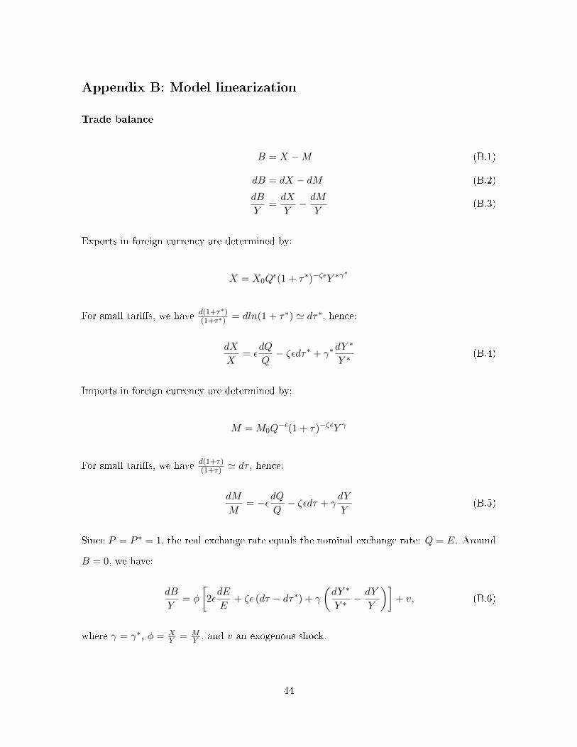
Appendix B: Model linearization
Trade balance
B = X −M (B.1)
dB = dX − dM (B.2)
dB
Y=dX
Y− dM
Y(B.3)
Exports in foreign currency are determined by:
X = X0Qε(1 + τ∗)−ζεY ∗γ
∗
For small tari�s, we have d(1+τ∗)(1+τ∗) = dln(1 + τ∗) ' dτ∗, hence:
dX
X= ε
dQ
Q− ζεdτ∗ + γ∗
dY ∗
Y ∗(B.4)
Imports in foreign currency are determined by:
M =M0Q−ε(1 + τ)−ζεY γ
For small tari�s, we have d(1+τ)(1+τ) ' dτ , hence:
dM
M= −εdQ
Q− ζεdτ + γ
dY
Y(B.5)
Since P = P ∗ = 1, the real exchange rate equals the nominal exchange rate: Q = E. Around
B = 0, we have:
dB
Y= φ
[2εdE
E+ ζε (dτ − dτ∗) + γ
(dY ∗
Y ∗− dY
Y
)]+ v, (B.6)
where γ = γ∗, φ = XY = M
Y , and v an exogenous shock.
44

Domestic output With C = cPYPc , I = I0(1 + r)−α, Pc = P 1−η(P ∗)η[E(1 + τ)]πη, and
P = P ∗ = 1, we have:
Y = c[E(1 + τ)]−ηπY + I0(1 + r)−α + EB (B.7)
dY
Y= c[E(1 + τ)]−ηπ
dY
Y− cηπE−ηπ(1 + τ)−ηπ
(dE
E+d(1 + τ)
(1 + τ)
)− αI0
Y(1 + r)−α
d(1 + r)
(1 + r)+BdE
Y
+ φE
[2εdE
E+ ζε (dτ − dτ∗) + γ
(dY ∗
Y ∗− dY
Y
)]+ v + u, (B.8)
where d(1+r)(1+r) = dln(1 + r) ' dr if r ' 0, and u is an exogenous shock.
We linearize around an initial equilibrium where τ ' 0, E = 1, r ' 0 and B ' 0:
dY
Y=− ηπc
1− c+ φγ
(dE
E+ dτ
)− αI
Y (1− c+ φγ)︸ ︷︷ ︸µ
dr
+φ
1− c+ φγ
(2εdE
E+ ζε (dτ − dτ∗) + γ
dY ∗
Y ∗
)+
v + u
1− c+ φγ(B.9)
After a shock, around the initial equilibrium (where B ' 0, τ = r = 0 and E = 1) we have
dBX = b, dτ = τ , dr = r and dE
E = dlnE = de = e. With dYY = y and dY ∗
Y ∗ = y∗, we get:
y = − ηπc
1− c+ φγ(e+ τ)− µr + φ
1− c+ φγ(2εe+ ζε(τ − τ∗) + γy∗) +
v + u
1− c+ φγ(B.10)
b = φ (2εe+ ζε(τ − τ∗) + γ(y∗ + y)) + v (B.11)
e = δ(r∗ − r) (B.12)
Calibration To calibrate µ, we re-write y so that it only depends on the two policy variables
r and τ , on the di�erent parameters and on the two shocks u and v:
45

y =−(− ηπc
1− c+ φγ+ µ+ 2εφ
)r +
(φζε− ηπc1− c+ φγ
)τ +
(2ζε− ηπc1− c+ φγ
)r∗
− φζε
1− c+ γφτ∗ +
φγ
1− c+ γφy∗ +
v + u
1− c+ φγ(B.13)
We thus have the following impact of τ and r on y and on b:
∂y
∂r= −
(µ+
2φε
1− c+ φγ− ηπc
1− c+ φγ
)(B.14)
∂y
∂τ=
(φζε
1− c+ φγ− ηπc
1− c+ φγ
)(B.15)
∂b
∂r=
(φ2ε(1− c− γ(1− φ))
1− c+ φγ− ηπc
1− c+ φγ+ γµ
)(B.16)
∂b
∂τ=
(φζε(1− c− γ(1− φ)) + γηπc
1− c+ φγ
)(B.17)
Then, we calibrate the impact of r on y based on the literature showing the impact of a rate
cut on US output. For an overall impact of 0.3 we have the following:
−(µ+
2φε
1− c+ φγ− ηπc
1− c+ φγ
)= −0.3
⇔ µ+0.1
0.36− 0.084
0.36= 0.3
⇔ µ = 0.26 ≈ 0.3 (B.18)
46

Appendix C
Figure 4: Optimal reaction of tari� depending on ζ
Note: policy responses to a negative demand shock of u = −1% in red, and to a negative trade shock v = −1%in blue. Source: model simulations.
47

Figure 5: Optimal reactions of interest rate depending on µ
Note: policy responses to a negative demand shock of u = −1% in red, and to a negative trade shock v = −1%in blue. Source: model simulations.
48