“tracking positive and negative effects of inequality on

Institut de Recerca en Economia Aplicada Regional i Pública Document de Treball 2014/01, 30 pàg. Research Institute of Applied Economics Working Paper 2014/01, 30 pag.

Grup de Recerca Anàlisi Quantitativa Regional Document de Treball 2014/01, 30 pàg.

Regional Quantitative Analysis Research Group Working Paper 2014/01, 30 pag.

“Tracking positive and negative effects of inequality onlong-run growth”

David Castells-Quintana and Vicente Royuela

Research Institute of Applied Economics Working Paper 2014/01, pàg. 2 Regional Quantitative Analysis Research Group Working Paper 2014/01, pag. 2

2

WEBSITE: www.ub-irea.com • CONTACT: [email protected]

WEBSITE: www.ub.edu/aqr/ • CONTACT: [email protected]

Universitat de Barcelona Av. Diagonal, 690 • 08034 Barcelona

The Research Institute of Applied Economics (IREA) in Barcelona was founded in 2005, as a research institute in applied economics. Three consolidated research groups make up the institute: AQR, RISK and GiM, and a large number of members are involved in the Institute. IREA focuses on four priority lines of investigation: (i) the quantitative study of regional and urban economic activity and analysis of regional and local economic policies, (ii) study of public economic activity in markets, particularly in the fields of empirical evaluation of privatization, the regulation and competition in the markets of public services using state of industrial economy, (iii) risk analysis in finance and insurance, and (iv) the development of micro and macro econometrics applied for the analysis of economic activity, particularly for quantitative evaluation of public policies.

IREA Working Papers often represent preliminary work and are circulated to encourage discussion. Citation of such a paper should account for its provisional character. For that reason, IREA Working Papers may not be reproduced or distributed without the written consent of the author. A revised version may be available directly from the author.

Any opinions expressed here are those of the author(s) and not those of IREA. Research published in this series may include views on policy, but the institute itself takes no institutional policy positions.


3

Abstract

Despite extensive research, there is still controversy on the effects of income inequality on economic growth. The literature proposes several transmission channels through which these effects may take place, and even the existence of two different forms of inequality. However, empirical studies have generally not distinguished between these channels, nor have their analyses included a consideration of the two forms of inequality and their separate effects on growth. In this paper we review the theory and the evidence on the different transmission channels through which inequality influences growth. We contribute to the literature by using a system of recursive equations, following a control function approach, to empirically assess the relevance of these channels and to differentiate between two forms of inequality. In this way we have captured in a single model not only a negative effect, but also a positive effect of inequality on long-run economic growth.

JEL classification: O1, O4 Keywords: inequality, economic growth, development

David Castells-Quintana. AQR Research Group-IREA. Department of Econometrics. University of Barcelona, Av. Diagonal 690, 08034 Barcelona, Spain. E-mail: [email protected] Vicente Royuela. AQR Research Group-IREA. Department of Econometrics. University of Barcelona, Av. Diagonal 690, 08034 Barcelona, Spain. E-mail: [email protected] ��


4

1. Introduction

Much has been said about the effects of income inequality on economic growth. The on-going debate rotates

around possible negative as well as positive effects of inequality on growth, characterized to work through different

transmission channels, and considering the complex nature of both phenomena. One factor seems to be of major

relevance; whether inequality is due to available opportunities and particular socio-economic and institutional

contexts, or due to market dynamics and unequal outcomes - and uneven success. The World Bank World

Development Report 2006 (WDR 2006) differentiates between equality of opportunities and equality of outcomes as two

parallel and differentiated components of inequality. While unequal opportunities are detrimental for development,

unequal outcomes generate necessary incentives for capital accumulation, innovation and economic growth;

“inequality of opportunity is wasteful and inimical to sustainable development and poverty reduction” but there is

an “important role of income differences in providing incentives to invest in education and physical capital, to work

hard, and to take risks (WDR 2006).” Similarly to WDR 2006, Easterly (2007) refers to “structural inequality” - due to

socio-institutional factors - and to “market inequality” - due to market forces. While the former relates to bad

institutions, low human capital investment and underdevelopment, the latter relates to uneven success in free

markets. Structural inequality is expected to have a negative effect on subsequent economic growth, while market

inequality is expected to have a positive effect.

More recently, the complex influence of inequality on the dynamics of economic growth has again attracted

attention of the scientific community after the world financial and economic crisis of 2008. Several authors have

placed a strengthened emphasis on the role of inequalities in the growth process of the last decades, but also on the

role of the dramatic rise of these inequalities in many countries as a cause of the crisis itself (Krugman 2008; Stiglitz

2009; Brescia 2010; Rajan 2010). According to these authors, currently high levels of inequality help to explain

evident deficiencies in terms of economic performance, which have accumulated over the long run.

In this paper we follow the literature on the different transmission channels for inequality to have an effect

on growth, and the idea of different components of inequality. By using several instruments - that we relate to the

different transmission channels - we decompose the variance of inequality using a system of recursive equations by

means of the Control Function Approach (CFA). Our aim is to further provide empirical evidence on the relevance

of the different transmission channels through which inequality operates. In particular, our contribution is the use of


5

the CFA to empirically assess the weight of the different mechanisms through which inequality affects economic

growth. Our first main finding is that inequality influences economic growth both positively and negatively.

Secondly, we argue that the negative influence accounts for roughly 80 per cent of the total effect. Thirdly, we found

that the role that each channel plays may depend critically on the circumstances of each country, with the negative

influence of inequality being significant in developing countries. These results are crucially important for policy

makers, as their challenge is to find out how, and not just if, inequality is affecting the process of economic growth.

The remainder of the paper is organized as follows. Section II briefly reviews the empirical evidence on the

effects of income inequality on economic growth, and also the theory and evidence on the different transmission

channels through which these effects occur. Section III sets out our model and empirical strategy. Section IV

presents the database. Section V displays the main results. Section VI performs several robustness checks. Finally,

section VII concludes.

2. The different effects of inequality on economic growth: literature review

The traditional econometric approach to assessing the overall impact of inequality on growth has introduced a single

measure of income distribution in an economic growth model.1 Along these lines, there is seemingly conflicting

evidence in the literature. On the one hand, several authors support the idea of a negative effect of inequality on

long-run growth (Alesina and Rodrik 1994; Persson and Tabellini 1994; Clarke 1995; Perotti1994, 1996; and Easterly

2007, among others). These results are based on cross-section analyses, an approach that, to the best of our

knowledge, has never provided evidence of a positive effect. On the other hand, other authors have found a positive

impact of inequality (Forbes 2000; Barro 2000; Chen 2003 and Voitchovsky 2005, among others). However, this

positive impact relies on panel data analysis and is either associated with short-term economic growth (Forbes 2000)

or is dependent on countries’ income (Barro 2000), on the initial income distribution itself (Chen 2003), on the

profile of inequality (Voitchovsky 2005), or on the process of urbanization (Castells-Quintana and Royuela 2011).

The main argument for using panel techniques is that they allow controlling for omitted time-invariant factors and

1 The most used measures are the Gini coefficients and the Theil indices. Some authors have also worked with different shares and ratios of the percentiles along the whole distribution of income. On one side, the percentage of the third quartile has been of particular interest to capture the weight of the middle class, on the basis that having a strong middle class boosts economic development (Easterly 2001; Partridge 2005). On the other side, the use of different percentile ratios allows for a focus on differentiated effects depending on the specific distributional forms of income (Voitchovsky 2005).


6

to address how a change in a country’s level of inequality will affect growth within that country (Forbes 2000).

When using fixed effects, however, if the underlying causal factors in the growth process are persistent, the long-run

cross-sectional effects will be subsumed into the fixed effects (Fallah and Partridge 2007). Indeed, as Forbes (2000)

highlights, it could be interesting to identify the time-invariant variables, omitted in panel analysis and that could

generate the negative bias in the inequality coefficient in cross-country growth regressions, as well as to evaluate the

different channels through which inequality, growth, and any other variables are related. Removing time-invariant

factors, which, as we will see, are precisely those to which the negative effect of inequality is related, limits the

possibility of empirically assessing the role of the different mechanisms behind the impact of inequality on growth.

In fact, Davis and Hopkins (2011) argue that panel techniques are not very informative about the relationship

between inequality and long-run economic growth, and suggest that the quality of economic institutions is the key

omitted variable that explains the negative effect of inequality on long-run growth.

The literature provides theoretical justifications for both a potential beneficial and a potential adverse effect

of inequality on the process of economic growth. In particular, while classical and neoclassical approaches have

underlined a beneficial effect of inequality on growth, modern perspectives highlight potential adverse effects of

inequality (Galor 2009). As our empirical aim is to identify differentiated negative and positive effects, we first

summarize how the different approaches predict a negative effect of inequality, and then demonstrate that a positive

effect can also be predicted.2

The negative effects of inequality on growth:

Up to five differentiated approaches have been identified to try to explain the mechanisms through which inequality

has a negative effect on long-run growth, which we briefly list:

1) One main transmission channel is through increased socio-political instability and risk of violent conflict,

which translates into uncertainty of property rights and reduces investment and growth (Alesina and Perotti 1996).

2 Ferreira (1999) presents “a brief overview to theories of growth and distribution”, including a review of three mechanisms that give rise to an effect of distribution on growth; political economy channels, capital market imperfections and social conflict channels. More recently, Ehrhart (2009) and Galor (2009) also present a short, though exhaustive and comprehensive overview of the theories and empirical evidence on the relationship between inequality and economic development. Neves and Silva (2013) provide a critical survey of the empirical literature trying to explain the sources of conflicting results.


7

Additionally, stability-threatening activities represent an unproductive waste of resources and reduce the overall

productivity of an economy (Barro 2000).

2) According to the political economy approach, either high inequality leads to higher redistributive pressure,

which in turn may lead to economic distortions and disincentives (Alesina and Rodrik 1994; Persson and Tabellini

1994), or leads the rich to lobby to prevent efficient redistribution policies from being implemented (Saint-Paul and

Vardier 1996; Bénabou 2002; Acemoglu and Robinson 2008). 3 These lobbying activities represent a waste of

resources related to rent seeking and corruption and precisely characterize what several authors have highlighted as

the fundamental adverse role of inequality in the current global crisis (Stiglitz 2009; Krugman 2012).

3) In a different way, the credit-market imperfections approach predicts that higher inequality reduces the capacity

of many individuals to invest when capital markets are imperfect and set-up costs are large. On one side this

increases macroeconomic volatility (Aghion et al. 1999), while on the other it reduces average investment - especially

in human capital (Galor and Zeira 1993). Both higher macroeconomic volatility and lower investment reduce long-

run growth.

4) The market size approach emphasizes the relevance of the middle class and the risks of lower aggregate

demand, derived from a higher proportion of population with lower purchasing power and the fact that lower

income groups tend to have higher propensity to demand local products (Murphy, Schleifer and Vishny 1989;

Todaro 1997).

5) Finally, the endogenous fertility approach highlights the link between higher inequality and higher fertility rates,

which in turn reduce growth. In particular, this happens given that as the number of children per family increases,

the average investment in education decreases (Barro 2000; Ehrhart 2009).

The positive effects of inequality on growth:

In parallel to the predicted negative effects, the literature also predicts possible positive effects of inequality through

different mechanisms.

3 Saint Paul and Verdier (1996) challenge the conventional political economy approach and argue that in fact unequal societies redistribute less and that this in turn is detrimental to growth. More recently, Woo (2011) has suggested a fiscal volatility channel for inequality to negatively influence growth.


8

1) The first of these mechanisms relates to a presumed greater propensity to save among the rich embodied

in classical and neoclassical models of growth. Along these lines, an increase in inequality leads to higher aggregate

savings and therefore to higher levels of investment and growth (Kaldor 1956), this effect being lower the more open

the economy is.

2) Moving into the modern perspectives, a second but related mechanism relies on the existence of large

set-up costs or investment indivisibilities, assumed in the capital market imperfections approach. Under these

investment indivisibilities, higher inequality again allows for greater aggregate investment (Aghion et al. 1999).

3) Furthermore, differentiating inequality of outcomes from inequality of opportunities, both classical and

modern perspectives acknowledge a growth-enhancing effect of inequality of outcomes. This growth-enhancing

effect relates to incentives for capital accumulation (Galor 2009) and for innovation (Mirrlees 1971), to incentives to

work hard and take risks (WDR 2006), and to agglomeration economies (Fallah and Partridge 2007; Castells-

Quintana and Royuela 2011).4

Examining each transmission channel

The above transmission channels have all been described in the related literature. Nevertheless, given data

constraints and the difficult task of separately measuring each channel, few studies have attempted to empirically

and independently assess each of the transmission channels through which inequality has a positive influence on

growth in some cases, but negative in others. Indeed, despite extensive evidence on the overall impact of inequality

on growth, a comprehensive empirical analysis and joint examination of the several transmission channels is still

missing in the literature. Those studies that have tried to analyse the dynamics of the transmissions channels have

usually focused on a single theoretical approach. The aim of these studies is to first see the relationship between

inequality and a given variable, as a proxy for the channel under analysis, to then see the effect of this variable on

growth (or variables that we know are relevant for growth, like investment). Appendix A lists the main papers

providing empirical evidence for the different channels, the variables they use as proxy for the channel, and the

effect they find either on growth or investment. Seminal works are Perotti (1994, 1996), Persson and Tabellini 4 Barro (2000) provides a good understanding of how some approaches predict at the same time a negative and a positive effect on growth. As Barro notes, even under the socio-political instability approach, lower inequality may not lead to higher growth. If economic resources are required for the poor to effectively threaten the socio-political stability, then income-equalizing transfers promote stability only to the extent that that they do not encourage the poor to involve in disruptive actions rather than work.


9

(1994) and Alesina and Perotti (1996). While the latter provides evidence on the negative role of socio-political

instability (using several variables for social unrest), the former test two other approaches, namely the capital-market

imperfections approach, using loan-to-value payment for mortgages as variable, and the political economy approach,

using the share of government transfers in GDP as a proxy for redistribution. However, none of these papers

considers the different channels in a single model. In a similar fashion to Alesina and Perotti, later studies have

focused on liberties, institutions and the quality of property rights as the main transmission channel within the

socio-political instability approach (Svensson 98; Keefer and Knack 2002). Persson and Tabellini (1994) focused on

the political economy approach, by considering welfare transfers on a small sample of 13 OECD countries for

which data were available, to find non-significant results about the prediction that inequality increases redistribution,

and that redistribution reduces growth. In fact, as noted before, other authors support a different relationship

between inequalities and redistributive polices.

Concerning the role of the domestic market, on the one hand Falkinger and Zweimmuller (1997) consider

product diversity, while on the other hand Keefer and Knack (2002) consider variables related to population,

aggregate GDP and openness. In both, results are not conclusively supportive of the domestic-market approach.

However, Davis (2008) has revalidated the relevance of scale effects, particularly in developing countries, and several

other authors have provided evidence of the relevance of the size of the middle class (Easterly 2001; Partridge

2005). Regarding the endogenous fertility approach, several studies provide evidence on the positive link between

inequality and fertility rates (Perotti 1996; Koo and Dennis 1999; Kremer and Chen 2002) and a negative effect of

fertility rates on growth (Barro 2000).5 Finally, although there is evidence of a positive effect of inequality, we have

not found in any paper any explicit assessment of the transmission channels related to this positive effect.

Can we see both effects of inequality on growth?

Unifying the classical and modern perspectives, Galor and Moav (2004) suggest a changing relationship between

inequality and growth depending on the process of development. Inequality is growth enhancing in early stages of

development, adverse afterwards in that process, and irrelevant in developed economies.6 Papers such as Barro

5 Yet, even controlling for fertility, Barro finds a negative effect of inequality in poor countries and a positive effect in rich countries. 6 In particular, in early stages of development, when physical capital accumulation is the prime engine for growth, inequality can enhance the process of development by channelling resources towards individuals whose marginal propensity to save is higher, allowing for higher levels


10

(2000), Chen (2003), Voitchovsky (2005), and Castells-Quintana and Royuela (2011) provide evidence that inequality

can have both negative and positive effects on economic growth, depending on the circumstances of the country.

Nevertheless, in these papers the two opposing effects are not empirically related to any of the different channels

through which inequality might affect growth, neither is there evidence of both effects happening simultaneously.7

Similarly, looking at two forms of inequality, Easterly’s (2007) empirical analysis focuses exclusively on structural

inequality, but no attempt is made at capturing market inequality and its relationship with economic development.

Summing up, although theoretically the relationship between inequality and growth works through different

channels, and although it is acknowledged that different forms of inequality are likely to have different effects on

economic growth, empirical evidence in this sense is still scarce. Few studies have attempted to isolate the multiple

channels of inequality. No paper, to the best of our knowledge, has captured separately, in a single model, two

different forms of inequality having opposing influences on long-run growth.8

III. Empirical Approach

Because the focus is on the long-run effects of income inequality, we followed the literature on the determinants of

cross-country differences on long-run economic growth. This literature tends to rely on OLS regressions of growth

rates using initial values of the explanatory variables, and results are interpreted as measuring the long-run effects of

those variables.9 In particular, we followed Sala-i-Martin et al.’s (2004) analysis on economic growth using cross-

of investment. In later stages of development, however, when human capital accumulation becomes the prime engine for growth, and given credit constraints, higher inequality leads to a lower spread of education among individuals, handicapping the process of development due to diminishing returns of human capital. Finally, as capital markets develop and credit constrains are relaxed, inequality becomes irrelevant. 7 Voitchovsky (2005) does find parallel positive and negative effects in a single model by using different parts of the income distribution; inequality at the top end of the distribution is positively associated with growth, while inequality lower down the distribution is negatively related to subsequent growth. However, the paper acknowledges that its empirical analysis “is not very informative regarding the different channels through which inequality might affect income.” 8 The closest study we found is Marrero and Rodriguez (2010). In line with our results, they find opposing effects for inequality of opportunities and for inequality of returns. Their study uses U.S. states panel data, rather than cross-county data, and does not consider empirically the different channels through which inequality has its effects. 9 Binder and Georgiadis (2011) note that the predominant tool used in the empirical output growth literature continues to be the “Barro regression”, using a cross section data set. They list up to four basic problems associated with these regressions: all cross country heterogeneities are assumed to be fully captured by the control variables; they are subject to endogeneity bias; there is no clear distinction between short and long run dynamics; and nonlinearities are not considered. All these arguments have been approached in the literature. The classification of countries and the introduction of interactions is a first strategy to deal with problems of heterogeneities and nonlinearities (Brock and Durlauf 2001; Durlauf et al. 2005). Another strategy is the use panel data sets and techniques. In this line, in the empirical literature on the effects of inequality on economic growth, the majority of cross sectional studies has found a negative coefficient (Dominicis et al 2008). On the contrary, when panel data sets are considered, the negative effects disappears and even becomes positive when fixed effects or GMM methods are used. Partridge (2005) has criticised the used of fixed effects methods for the analysis of such relationship, as inequality is a highly persistent variable over time. Similarly, Barro (2000) maintains that fixed effects estimates exacerbate the bias due to measurement error. In our paper, we try to integrate into a cross section framework both the positive and negative effects of inequality on economic growth focusing on long-run dynamics (as we average growth over 37 years).


11

sectional data. We set a neoclassical econometric model of economic growth (equation (1)) where is our

dependent variable, reflecting cumulative annual average GDP growth rate (in per capita terms), is income

inequality, and is a list of control variables, including the initial income, :

(1)

OLS regressions are likely to underestimate the negative effect of inequality, and this could be indeed because of a

co-occurring positive effect (Easterly 2007). In fact, reduced form estimations for the effect of inequality on growth

are likely to pick up different effects at the same time (Bourguignon 1996), related to the above-discussed

transmission channels. A common strategy in the empirical literature reviewed has been the use of intermediate

variables as proxies for the channel under analysis. In parallel, taking into account endogeneity concerns on the

effect of inequality on growth and the existence of two differentiated components of inequality, a second approach

has been to isolate one of those components using specific instruments for inequality (as in Easterly 2007). Both

strategies, therefore, rely on the use of instrumental variables to capture a particular component of inequality or

mechanism through which inequality has an effect on growth. In the first strategy each channel is considered

independently and no attempt is made to examine all of them in a single growth model. In fact, as we have seen, few

papers consider empirically more than a single channel. Similarly, in the second strategy only the structural

component, leading to a negative effect of inequality on growth, is considered empirically. Building on both

strategies, our goal was to assess the relevance of each transmission channel by using the different variables

proposed in the literature, and to differentiate between two forms of inequality in its relationship with long-run

economic growth.

Following the literature, we considered inequality as an endogenous variable in equation (1). One solution

for dealing with endogeneity is to apply the so-called Control Function Approach. Like instrumental variables

(2SLS), this procedure uses instruments to break the correlation between endogenous explanatory variables and

unobservable variables affecting the response. In linear models with one endogenous regressor, CFA yields identical

results to those obtained with 2SLS. CFA, therefore, yields consistent parameter estimates if instruments are valid

(Imbens and Wooldridge 2009 and Wooldridge 2010).


12

Following Wooldridge's (2010) formalization of the CFA, we considered a list of instruments for inequality,

, that are exogenous in model (1):

(2)

where in model (1) is a strict subset of . As in 2SLS, we considered the reduced form for inequality as:

(3)

(4)

Since is uncorrelated with , it turns out that is endogenous in (1) if and only if . The

linear projection of onto in error form is:

(5)

Since both and are orthogonal to , then , and is exogenous if and only if .

Plugging equation (5) into equation (1) transforms our growth equation into:

(6)

where, by construction, is uncorrelated with , and . As we cannot observe , the solution under

the CFA is to estimate - the residual from an OLS regression of equation (3). Replacing with in (6) and

estimating again by OLS yields consistent estimates for , and . The parameter in (6) will capture the bias

that would affect if we did not control for , allowing us to see the sign and magnitude of that bias.

Now, if we assume that our instrument set - in equation (2) - only captures a negative form of inequality,

the remaining unexplained variance of inequality, including its positive form, is captured by . In other words, as

far as we can capture the negative component of inequality by , the remaining variance of inequality will most likely

be an approximation of its positive component. Consequently, the parameter in an OLS estimation of equation

(6), once the original values of and the estimations of , namely , are included, can be interpreted as a proxy

estimation of the positive association between inequality and long-run economic growth.10 The use of instruments

10 In fact, we could consider inequality as , where only the negative component can be captured with healthy instruments ( ), while the positive component can only be captured through covariates, , that are correlated with . Hence, the residual of the linear projection of on , , would equal , and the linear projection of onto in error form would be

. Consequently, the remaining estimated component in our growth equation would include plus any unexplained variance, . In this case, would consistently estimate the negative influence of inequality on economic growth. It can happen, though, that some mechanisms of inequality are at the same time related to their positive and to their negative associations with growth, as suggested in the literature, and consequently . In such case, the estimation of in (3) would not equal , being the bias linked


13

to identify channels, together with the residual variation in recursive estimation, has been used in the

macroeconomic literature (e.g. Bruckner 2012). As far as we know, however, it is the first time it has been used for

inequality.11

IV. Data

As control variables in our growth model we used log_pcgdp - the initial level of per capita GDP (in log), life_exp - the

life expectancy at birth, p60 - the primary enrolment rate, yrsopen - the number of years the economy has been open

between 1950 and 1994, primary_exports - the fraction of primary exports in total exports, and mining - the fraction of

GDP in mining - to capture natural endowments.12 The data, aside that for income inequality, comes from Sala-i-

Martin et al. (2004), the Penn World Table (PWT), and the World Bank Development Indicators database. Income

inequality is measured by the Gini coefficient, and we relied on Gruen and Klasen (2008).13 (A table with the

variables used and their sources is annexed as Appendix B). We used data as close to 1970 as possible to explain

average growth rates between 1970-2007 in a sample of 51 countries (a list of which is also annexed as Appendix

C).14

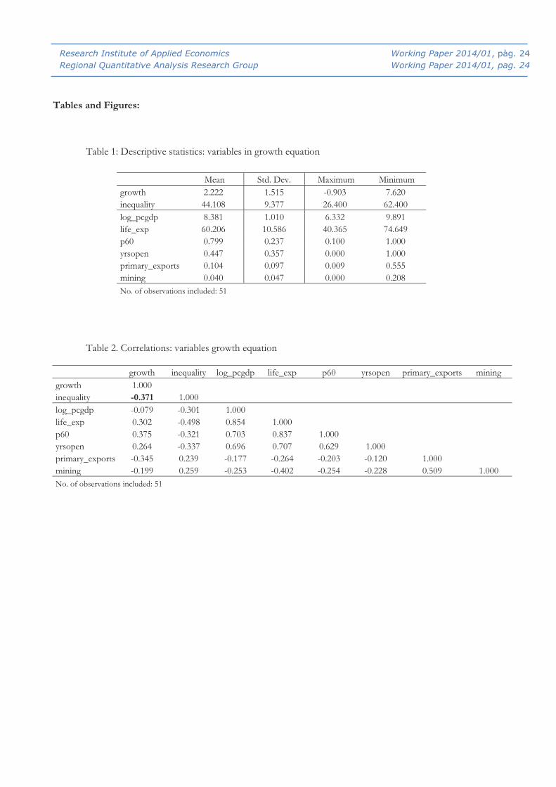
Table 1 presents descriptive statistics for the variables used in the growth equation, while Table 2 presents

correlations among the variables. Growth is positively correlated with initial values of life_exp, p60 and yrsopen. By

contrast, growth is negatively correlated with initial values of log_pcgdp, primary_exports, mining and inequality. In fact,

the highest negative correlation (-0.371) is of growth with inequality. Regarding inequality and the controls, inequality

is positively correlated with mining and primary_exports and negatively correlated with all the other variables.

to As a consequence our approach would be affected and we could expect a bias towards zero of both and in (6). Subsequently, we understand that the misspecification in (3) coming from not considering instruments of the positive channel of inequality,

, that could be correlated with the instruments of negative channels, , would be driving our estimates in (6) to be non-significant. Hence, if we find significant results for both and ,we will be able to say that they are downward bounded. 11 Bruckner (2012), however, aims at differentiating two causal effects running in opposite directions. Our aim is to differentiate the different signed relationships between inequality and long-run economic growth. 12 Out of 67 possible explanatory variables, Sala-i-Martin et al. (2004) found 18 that were significantly related to long-run growth during 1960-1996. Results suggest that main determinants for growth include initial levels of per capita GDP - the neoclassical idea of conditional convergence - and variables for natural resource endowments, physical and human capital accumulation, macroeconomic stability, and productive specialization. A negative and significant effect was found for the fraction of primary exports in total exports. 13 These coefficients were adjusted from the WIID database for different possible objects of measure and related to households or families and for the entire population, allowing us to address concerns about international comparability of inequality data. These adjusted coefficients have previously been used by us as well as by other authors (e.g. Atkinson and Brandolini 2010). We relied on income, rather than land or wealth, inequality, because it is income distribution that possibly reflects two distinct sources of inequality, namely inequality of opportunities and inequality of returns, which influence economic growth in opposite directions (Neves and Silva 2013). 14 The selected countries are those for which reliable data for all the variables used here has been found. The sample includes major countries from all world regions.


14

Table 1. Descriptive statistics: variables in the growth equation

Table 2. Correlations: variables in the growth equation

Additionally, we looked for variables related to inequality that we could use to identify each of the

transmission channels that give rise to an effect on long-run economic growth. For Socio-Political Instability (SPI)

we considered variables related to social unrest and violence, following Alesina and Perotti (1996). We used a

parsimonious strategy and selected, among several variables positively correlated with inequality and negatively with

growth, three variables that yielded the highest R-square in a regression on inequality.15 For redistributive policies, as

one main focus of the Political Economy (PE) approach, we used average government spending and average

expenditure on education, both as share of GDP. Regarding the Credit Market Imperfections (CMI) approach, we

considered access to sound money and patents, as proxies for innovation. For Domestic Market size and the role of

the middle class (DM) we used aggregate GDP and the share of the third quintile in the income distribution. Using

openness as one of the controls in the growth equation already captures the role of foreign markets. For the role of

Fertility decisions (FER) we considered population growth rates, infant mortality rates, and the proportion of family

farms, all highly correlated with fertility rates and inequality levels.16 As with controls in the growth equation, we

considered data as close to 1970 as possible. We added to our list of variables, time-invariant variables expected to

capture the structural component of inequality (SI):17 the exogenous suitability of land for wheat versus sugarcane -

as proxy for factor endowment differentials across countries - and the proportion of population in tropical areas, as

15 We also considered several other variables for social unrest and violence as robustness checks in the estimations described in section 4. Aside from social unrest and violence, other authors have considered variables related to liberties, rights and institutions. However, data for these variables are only available from the 80s and are expected to by highly affected by economic performance. We therefore restricted our analyses to the selected variables, which are some of the most commonly used in the literature and helped to reduce endogeneity. 16 When we regressed inequality on our controls, fertility rates did not add significant explanatory power, and their use as a valid instrument for inequality was rejected by the instrument tests implemented. 17 It is important to highlight the difference between the variables that we used for each transmission channel and the instruments for structural inequality. The latter are predetermined time-invariant exogenous variables expected to capture factor endowments, while the rest of our variables are time-variant. In this line, we looked for variables measured as close as possible to 1970 and which, although not predetermined, could be considered as exogenous in the growth equation. What we were trying to do, in accordance with the empirical strategy set in section III, was to simply use them to capture specific and differentiated mechanisms of the impact of inequality on growth.


15

considered by Easterly (2007), and the proportion of mountainous lands, as used by Collier (2009). 18 Table 3

presents descriptive statistics for all the different variables considered as instruments and their correlation with

inequality.

Table 3: Descriptive statistics: instruments

V. Estimation and Results

We implemented our empirical strategy by recursive estimation. In a first equation we estimated income inequality

by using different instruments according to transmission channel (as in equation 3). From this first estimation we

generated for each set of instruments, an estimated residual term, , capturing the unexplained variance in

inequality. Because we are assuming that inequality has an effect on growth through different channels that can be

associated with different components of this inequality (Easterly 2007; WDR 2006), this residual is expected to

capture other components of inequality that are not associated with the variables used as instruments. In a second

equation, and again for each set of instruments, we introduced inequality and the estimated residual from the first

equation, along with control variables, in order to estimate our model of long-run economic growth. By introducing

both terms, i.e. inequality and the estimated residual, we were able to assess the effects of two different components

of inequality on economic growth. By using different sets of instruments, we could analyse which factors needed to

be controlled for our residual to capture a long-run growth-enhancing component of inequality. This is something

that is not done in panel data analysis, which suggests a positive effect of inequality on growth. In particular, we

expected to differentiate between negative and positive effects when we considered as instruments in the first

equation all of those variables that we had related to a negative component of inequality.

Table 4 presents the results from estimating equation (3), in which we regressed inequality on different sets

of instruments, including controls from the growth equation. We report standardized (beta) coefficients and Shea’s

Partial R-square to measure the relevance of the considered instruments excluded from the growth equation. When

we included all instruments for structural inequality, plus all the others related to a negative effect of inequality, we

18 Collier considered the proportion of mountainous land as a determinant of the probability of conflict, in which he discarded inequality as a relevant factor.


16

could explain about 80 per cent of the variance in inequality (column 7). It is important to note the relevance of the

instruments considered as proxy for structural inequality, yielding a partial R-square of 0.489. In particular, and

interestingly enough, the proportion of mountainous land - a factor not considered before in the literature as an

instrument for inequality - has a high correlation with inequality. Moreover, the proportion of mountainous land

remains highly significant even when controlling for other proxies for structural inequality. In any case, most of

these structural factors are time-invariant factors that are cancelled out in the panel data analysis with fixed effects or

first differences. This explains why a positive effect of inequality is found in this type of analysis.

Table 4: Results for the inequality equation

Before we assessed our two components in the growth equation, we tested to what extent they indeed

captured negative and positive dynamics in the growth process, based on the theory revised in section II. One

simple and straightforward way is to see how the two components correlate with long-run growth, as well as with

physical and human capital accumulation, innovation and institutional quality. On the one hand, our estimated negative

inequality (i.e. predicted values for inequality when we consider all the different instruments related to a negative

effect) has a significant negative correlation with growth, -0.462, as well as with the average investment during the

whole period (ki), -0.247, and with the total average years of schooling in 2005 (schooling), -0.429. The correlation

with innovation and institutional quality (icrg_qog) are also negative, -0.517 and -0.578, respectively. On the other

hand, our second component has a positive correlation with growth, 0.117, as well as with physical capital

accumulation, 0.191. Figure 1 plots our two orthogonal components and their relationship with long-run growth.

Both components have been standardized to split the sample of countries in four quadrants. It can be seen that

countries with lower estimated negative inequality had higher growth rates (represented with bubbles higher in the

graph). Furthermore, the highest average growth rates were found in the top left quadrant of the figure. In this

quadrant we find countries with low estimated negative inequality but a high estimated residual (our positive

component); e.g. Denmark, Hungary, Ireland, South Korea and the United States. By contrast, the lowest average

growth rates were found in countries with high estimated negative inequality but a low estimated residual (the


17

bottom right quadrant, including mostly Latin American countries like Peru and El Salvador, but also other

countries like Zambia and Cote d’Ivoire).

Figure 1: Two components of inequality and long-run growth

Table 5 presents results for the impact of inequality on long-run growth. Column 1 shows the results from

the OLS estimation of model (1). The remaining columns present the results from our 2SRI (two-stage residual

inclusion) estimations (Terza et al. 2008), where we introduced as a further control in the growth equation the

residual from the first set of estimation for inequality (as suggested by the CFA). Estimations were done using

bootstrap standard errors to adjust for the generated regressor bias from the first equation. We report the

Kleibergen-Paap LM test probability to check for under-identification, and the Hansen test probability to check for

the validity of instruments.19

Table 5: Results for the growth equation

All controls have the expected sign in all estimations and their coefficients are all significant (except for that

of mining). Results are consistent with conditional convergence, with a negative coefficient for initial per capita

GDP of around 2 per cent - as in Sala-i-Martin 2004 - and higher human capital levels increasing long-run growth

(i.e. a positive coefficient for life_exp and p60). Openness is also positively associated with growth, while primary

sector specialization is negatively so (i.e. a negative coefficient for primary_exports). For inequality, the OLS

estimation yields a negative, although non-significant, coefficient. As aforementioned, this could be the result of two

significant effects cancelling each other out.20 When we further controlled for the two differentiated components,

the coefficient for inequality became significant in some of the estimations. In particular, the sets of instruments for

domestic market (estimation 2SRI (4)) and the set for structural inequality (estimation 2SRI (6)) yield in both cases a

19 In fact, we tested for the relevance and validity of our instruments in different ways. For relevance, we looked at the F statistic and the Partial-R-squared of the first regression, and performed under-identification tests. For validity we performed over-identification tests. In Table 4 we report the Kleibergen-Paap LM statistic test and the Hansen J test. 20 We tested for the endogeneity of inequality. While Durbin and DWH tests reject the null hypothesis of no endogeneity, the Wooldridge test, which considers robust standard errors, did not (but with a p-value of 0.12, still close to suggesting endogeneity).


18

significant and negative coefficient for inequality. Likewise for the set in which we included all the instruments for

structural inequality plus all the others related to a negative effect of inequality - excluding those regarded as invalid

by the performed tests (estimation 2SRI (7)). Interestingly, the coefficient for our forecasted residual, which captures

the remaining variance in inequality not explained by the instruments considered, is positive and significant only

when we control for the domestic market mechanism or for all the instruments related to a negative effect of

inequality on growth. As we saw above (see footnote 10) any bias in our procedure for not considering the full set of

instruments would lower towards zero the estimates of both components. Consequently, the results in column 7 are

not only significant, but also downward-bounded, reinforcing our intuition.

These results support previous results of a negative effect of inequality, in particular related to the role of

the size of the domestic market and the middle class, or to structural factors. Furthermore, our results support the

idea of two differentiated components of inequality, associated with two different-signed effects. Nevertheless, these

two parallel effects only become evident when the differentiated mechanisms for inequality are appropriately

controlled for. Regarding the total impact of inequality, the OLS estimation in column 1 yields a net impact of

inequality of 0.015. By contrast, controlling for two different components of inequality yields a negative effect of -

0.038 and a positive effect of 0.083. However, considering that our negative component of inequality captured

around 80 per cent of the variance in inequality, with the residual capturing the remaining variance, the weighted

average of the two can be approximated to -0.017. This is close to the value reported in column 1 and results in

previous studies, and an economically significant effect after considering the wide differences in the Gini

coefficients among countries. The difference between the country with the highest inequality in 1970, Honduras,

and the country with the lowest, Hungary, can represent a difference of half a point of average annual growth.

Results by level of development

Is there always a positive effect of inequality on economic growth? According to Galor and Moav (2004), as we have

seen, the relationship between inequality and growth changes with the stage of development and is expected to be


19

positive only in early stages, and non-significant in developed economies.21 However, Galor and Moav’s analysis

focuses on the role of credit market imperfections. However, we have seen that there are other channels at work.

Thus, we can still have a positive effect of inequality at early stages of development, as suggested by Galor and

Moav, but also a negative effect, as suggested by other approaches. We performed structural stability tests on our

sample by differentiating countries based on whether they were OECD members in 1970 or not, as a proxy for

stage of development.22 As the tests support the possibility of differentiated effects, in Table 6 we let the impact of

our two components of inequality to vary for countries that were OECD members in 1970 and for countries that

were non-members.23 All controls remained significant, except that for mining. Additionally, once we controlled for

two components of inequality, the negative and positive effects of inequality are only significant in developing

countries. For developed countries the two components still have coefficients with opposing signs, although they

are non-significant (in line with Galor and Moav 2004).24

Table 6: Results by level of development

VI. Sensitivity and Robustness Checks

Because our procedure relies heavily on the selection of instruments, a first check of our results was to use a

different set of instruments for each of the channels. For most channels this is complicated because of data scarcity.

However, as noted before, we do have several variables that could be used to capture the idea of socio-political

instability. We tried the variables considered by Alesina et al. (1996, political instability dataset), although at the

expense of losing 4 observations due to data availability. However, we were still able to find significant coefficients

(one positive and one negative) for our two components of inequality (see estimation 1 in Table 7).

As a second check of our results, we analysed the possibility of direct effects on economic growth that were

not associated with inequality of some of the channels considered. In particular, fertility rates are expected to have a

21 Indeed, the previously studied correlations of our two components of inequality with growth and capital accumulation become stronger if we consider separately the developing and the developed countries. 22 In particular, we tested parameter heterogeneity for the coefficients for our two components of inequality based on the OECD-non-OECD dichotomy. 23 Thus, we expect to partly control for heterogeneity across countries. 24 Chambers and Krause (2010) provide evidence of the second phase of Galor and Moav’s (2004) hypothesis; in particular that in countries with low educational attainments, the negative effects of inequality increase with higher capital stocks.


20

direct and negative effect on long-run growth, associated with family decisions relevant for physical and human

capital accumulation (Barro 2000). We controlled for fertility rates directly in the growth equation (see estimation 2

in Table 7). The coefficient for fertility is negative and significant, as expected. However, even after controlling for

fertility we found two significant effects of inequality on growth. Barro found a non-significant effect for inequality

after controlling for fertility, but did not consider, as we did, further opposing and significant effects of inequality

that could be cancelling each other out.

As with fertility, we expanded our analysis to the consideration of the direct roles of other transmission

channels in the growth equation. For our first channel under consideration we followed Alesina and Perotti (1996)

and constructed an index as proxy for socio-political instability (SPI index), using the method of principal

components analysis applied to several variables of social unrest. For redistributive policies we introduced the

variable share of government consumption over GDP (kg), which captures government spending. For the role of

the domestic market we introduced the initial income (logGDP1970), capturing domestic market size, and to quantify

the role of the middle class, we included the share of the third quintile in the income distribution (Q3). Finally, we

maintained fertility rates as a further control. Once we had controlled for all the transmission channels that yielded a

negative effect of inequality on growth, our second component remained positive and significant (estimation 3 of

Table 7).

Table 7: Robustness checks

VII. Discussion and Conclusions

We introduce the use of the control function approach (CFA) to address endogeneity concerns in the effect of

inequality on economic growth. The CFA has allowed us to track different transmission channels of the effects of

inequality on long-run economic growth, by using alternative sets of instruments. By considering the idea of two

differentiated components of inequality (WDR 2006) and different proxies expected to relate to different

transmission channels, we have empirically distinguished in a single model both negative and positive effects of

inequality on long-run growth. Our results suggest, in line with the literature, that high inequality has indeed a

negative effect on long-run growth, very likely by increasing social unrest and political instability, by lowering


21

aggregate demand, and given its relationship with higher fertility rates. However, our results also support the

possibility of a long-run growth-enhancing component of inequality, and allow us to see the relevance of the

mechanisms that need to be controlled for that positive effect of inequality to become empirically evident.

Results emphasize the complexity of the relationships between income distribution and economic growth.

This complexity exists everywhere but is more intense in developing countries. In this manner, what is interesting is

not whether inequality is harmful or beneficial for growth but rather to attain a satisfactory description of the

dynamics of the relationship in these countries. In order to assess the impact of inequality on economic growth in a

given country, one should focus on analyzing what is driving inequality. When inequality is structural and associated

with political instability and social unrest, rent-seeking and distortive policies, lower capacities for investments in

human capital and a stagnant domestic market, it is mostly expected to harm long-run economic performance, as

suggested by many authors. Accordingly, improving income distribution is expected to foster long-run economic

growth, especially in low-income countries, where the levels of inequality are usually very high. However, some

degree of inequality can also be good, as has been theoretically argued before in the literature and as empirically

suggested in this study. A degree of inequality, when driven by market forces and related to hard work and growth-

enhancing incentives, like risk taking, innovation, capital investments and agglomeration economies, can play a

beneficial role for economic growth. The challenge for policy makers is to control structural inequality that reduces

the country´s capacities for economic development, while at the same time keeping in place those positive incentives

that are also necessary for growth. To ease this task, a broader and deeper understanding of the dynamics behind the

relationship between inequality and economic development will prove to be invaluable.


22

REFERENCES

Acemoglu, D. and Robinson, J.: Persistence of power, elites and institutions. American Economic Review 98(1), 267-293 (2008) Alesina, A. and Rodrik, D.: Distributive politics and economic growth. The Quarterly Journal of Economics 109, 465-490 (1994) Alesina, A., Özler, S., Roubini, N., and Swagel, P.: Political instability and economic growth. Journal of Economic Growth 1, 189-

211 (1996) Alesina, A. and Perotti, R.: Income distribution, political instability, and investment. European Economic Review 40, 1203-1228

(1996) Aghion, P., Caroli, E. and García-Peñalosa, C.: Inequality and Economic Growth: The Perspective of New Growth Theories.

Journal of Economic Literature Vol. 37 No. 4, 1615-1660 (1999) Atkinson, A. and Brandolini, A.: On analyzing the World Distribution of Income. The World Bank Economic Review 24(1), 1-37

(2010) Barro, R. J.: Inequality and growth in a panel of countries. Journal of Economic Growth 5, 5-32 (2000) Barro, R. J., and Lee, J.W.: International Comparisons of Educational Attainment. Journal of Monetary Economics 32, 363-394

(1993) Benabou, R.: Tax and Education Policy in a Heterogeneous-Agent: What Levels of Redistribution Maximize Growth and

Efficiency? Econometrica, Econometric Society, 70(2), 481-517 (2002) Binder, M. and Georgiadis, G.: Determinants oh Human Development: Capturing the Role of Institutions. CESIFO Working

Paper No. 3397. (2011) Bourguignon, F.: Equity and economic growth: permanent questions and changing answers? Document de trevail No 96-15,

DELTA, Paris (1996) Brescia, R.: The cost of inequality: Social Distance, Predatory Conduct, and the Financial Crisis. NYU Annual Survey of American

Law, Vol. 66 (2010) Brock, W. A. and Durlauf, S.: Growth empirics and reality. World Bank Economic Review 15, 229-272 (2001) Bruckner, M.: Economic growth, size of the agricultural sector, and urbanization in Africa. Journal of Urban Economics 71, 26-36

(2012) Castells-Quintana, D. and Royuela, V.: Agglomeration, Inequality and Economic Growth. IREA-WP series, no. 2011/14 (2011) Chambers, D. and Krause, A.: Is the relationship between inequality and growth affected by physical and human capital

accumulation? Journal of Economic Inequality 8, 153-172 (2010) Chen, B.: An inverted-U relationship between inequality and long-run growth. Economics Letters 78, 205-212 (2003) Clarke, G.: More evidence on income distribution and growth. Journal of Development Economics 47, 403-427 (1995) Collier, P.: Beyond greed and grievance: feasibility and civil war. Oxford Economic Papers 61, 1-27 (2009) Davis, L.: Scale effects in growth: A role for institutions. Journal of Economic Behavior & Organization, Vol. 66, 403-419 (2008) Davis, L. and Hopkins, M.: The institutional foundations of inequality and growth. Journal of Development Studies 47(7), 977-997

(2011) De Dominicis, L., Florax, R. and de Groot, H.: A meta-analysis on the relationship between income inequality and economic

growth. Scottish Journal of Political Economy, Vol. 55, No. 5, 654-682 (2008) Durlauf, S., Johnson, P. and Temple, J.: Growth Econometrics. In Philippe Aghion and Steven Durlauf (eds.), Handbook of

Economic Growth, Elsevier: 255-677 (2005) Ehrhart, C.: The effects of inequality on growth: a survey of the theoretical and empirical literature. ECINEQ Working Paper

Series 2009-107 (2009) Easterly, W. (2001): The Middle Class Consensus and Economic Development. Journal of Economic Growth 6, 317-335 (2009) Easterly, W.: Inequality does cause underdevelopment: insights from a new instrument. Journal of Development Economics 84, 755-

776 (2007) Falkinger, J. and Zweimuller, J.: The impact of income inequality on product diversity and economic growth. Metroeconomica

48(3), 211-237 (1997) Fallah, B. and Partridge, M.: The elusive inequality-economic growth relationship: are there differences between cities and the

countryside? Annals of Regional Science 41, 375-400 (2007) Ferreira, F.: Inequality and Economic Performance: A Brief Overview to Theories of Growth and Distribution. The World Bank, Washington,

DC. (1999) Forbes, K.: A reassessment of the relationship between inequality and growth. The American Economic Review 90(4), 869-887

(2000) Galor, O.: Inequality and Economic Development: The Modern Perspective. Edward Elgar Publishing Ltd. (2009) Galor, O. and Moav, O.: From Physical to Human Capital Accumulation: Inequality and the Process of Development. Review of

Economic Studies 71(4), 1001-1026 (2004) Galor, O. and Zeira, J.: Income distribution and macroeconomics. The Review of Economic Studies, Vol.60, No. 1, 35-52 (1993) Gruen, C. and Klasen, S.: Growth, inequality, and welfare: comparisons across time and space. Oxford Economic Papers 60, 212-

236 (2008)


23

Hall, R. and Jones, Ch.: Why do some countries produce so much more output per worker than others? Quarterly Journal of Economics 114(1), 83-116 (1999)

Heston, A. Summers, R. and Bettina, A.: Penn World Table Version 7.1. Centre for International Comparisons of Production, Income and Prices. University of Pennsylvania (2012)

Lutz, W., Goujon, A. KC, S. and Sanderson, W.: Vienna Yearbook of Population Research 2007. International Institute for Applied System Analysis of the Vienna Institute of Demography (2007)

Imbens, G.W. and Wooldridge, JM.: New developments in Econometrics. Cemmap Lecture Notes 14 (2009) Kaldor, N.: Alternative Theories of Distribution. The Review of Economic Studies, Vol. 23, No. 2, 83-100 (1956) Keefer, P. and Knack, S.: Polarization, politics and property rights: Links between inequality and growth. Public Choice, Vol. 111,

127-154 (2002) Kremer, M. and Chen, D.: Income Distribution Dynamics with Endogenous Fertility. Journal of Economic Growth 7, 227-258

(2002) Krugman, P.: The return of depression economics and the crisis of 2008. Penguin. London (2008) Krugman, P.: End this depression now! Norton. London (2012) Koo, L. and Dennis, B.: Income inequality, fertility choice and economic growth: theory and evidence. Harvard Institute for

International Development (HIID), Development Discussion Paper No 687, March (1999) Marrero G., and Rodriguez, J.: Inequality of opportunity and growth. Journal of Development Economics 104, 107-122 (2010) Mirrlees, JA.: An exploration in the theory of optimum income taxation. The Review of Economic Studies, Vol. 38, No 2, 175-208

(1971) Murphy, K. Schleifer A. and Vishny, R.: Income distribution, market size, and industrialization. Quarterly Journal of Economics,

Vol. 104(3), 537-564 (1989) Neves, P.C., and Silva, S.M.T.: Survey article: Inequality and growth. Journal of Development Studies. DOI:

10.1080/00220388.2013.841885(2013) Partridge, M.: Does income distribution affect U.S. state economic growth? Journal of Regional Science 45, 363-394 (2005) Perotti, R.: Income distribution and investment. European Economic Review 38, 827-835 (1994) Perotti, R. (1996). Growth, income distribution and democracy: what the data say? Journal of Economic Growth 1, pp. 149-187. Persson, T. and Tabellini, G.: Is Inequality Harmful for Growth? Theory and evidence. American Economic Review 84, 600-621

(1994) PRS Group.: International Country Risk Guide Researchers Dataset. Data Web Site: http://hdl.handle.net/10864/10120 PRS

Group [Distributor] V3 [Version] (2012) Rajan, R.: Fault Lines: How hidden fractures still threaten the world economy, Princeton University Press. (2010) Sachs, J. and Warner, A.: Economic reform and the process of economic integration. Brookings Papers on Economic Activity 1, 1-95

(1995) Sachs, J. and Warner, A.: Natural resource abundance and economic growth. CID at Harvard University. Data Web Site:

www.cid.harvard.edu/ciddata.html. (1997) Saint-Paul, G. and Verdier, T.: Inequality, redistribution and growth: A challenge to the conventional political economy

approach. European Economic Review (40), 719-728 (1996) Sala-i-Martin, X., Doppelhofer, G. and Miller, R.: Determinants of long-term growth: A Bayesian averaging of classical

estimates (BACE) approach. American Economic Review 94(4), 813-835 (2004) Stiglitz, J.: The global crisis, social protection and jobs. International Labour Review Vol. 148, No. 1-2, 1-13 (2009) Svensson, J.: Investment, property rights and political instability: Theory and evidence. European Economic Review (42), 1317-1341

(1998) Terza, J., Basu, A. and Rathouz, P.: Two-Stage Residual Inclusion Estimation: Addressing Endogeneity in Health Econometric

Modelling. Journal of Health Economics 27, 531-543 (2008) Todaro, MP: Economic Development. London: Longman (1997) Voitchovsky, S.: Does the profile of income inequality matter for economic growth? Distinguishing Between the Effects of

Inequality in Different Parts of the Income Distribution. Journal of Economic Growth 10(3), 273-296 (2005) Woo, J.: Growth, income distribution, and fiscal policy volatility. Journal of Development Economics 96(2), 289-313 (2011) Wooldridge, JM.: Econometric Analysis of Cross-Section and Panel Data (Second Edition). MIT Press: Cambridge, MA. (2010) World Bank: Equity and Development, World Development Report 2006. World Bank, Washington DC. (2006)


Tables and Figures:

Table 1: Descriptive statistics: variables in growth equation

Mean Std. Dev. Maximum Minimum growth 2.222 1.515 -0.903 7.620 inequality 44.108 9.377 26.400 62.400 log_pcgdp 8.381 1.010 6.332 9.891 life_exp 60.206 10.586 40.365 74.649 p60 0.799 0.237 0.100 1.000 yrsopen 0.447 0.357 0.000 1.000 primary_exports 0.104 0.097 0.009 0.555 mining 0.040 0.047 0.000 0.208 No. of observations included: 51

Table 2. Correlations: variables growth equation

growth inequality log_pcgdp life_exp p60 yrsopen primary_exports mining growth 1.000 inequality -0.371 1.000 log_pcgdp -0.079 -0.301 1.000 life_exp 0.302 -0.498 0.854 1.000 p60 0.375 -0.321 0.703 0.837 1.000 yrsopen 0.264 -0.337 0.696 0.707 0.629 1.000 primary_exports -0.345 0.239 -0.177 -0.264 -0.203 -0.120 1.000 mining -0.199 0.259 -0.253 -0.402 -0.254 -0.228 0.509 1.000 No. of observations included: 51


Table 3. Descriptive statistics: variables inequality equation

Channel / Instrument Mean Std. Dev. Min Max Corr. with Inequality

SPI assassp2 0.005 0.021 0.000 0.138 0.254 death 12.102 4.365 5.678 23.500 0.173 wardum 0.392 0.493 0.000 1.000 0.265

Political Economy kg702007 8.593 4.264 2.221 20.918 0.020 exp_edu 15.070 4.403 6.187 24.478 0.358

CMI fi_sm 7.017 1.608 2.518 9.647 -0.029 innovation 74.704 124.992 0.000 539.986 -0.492

Domestic Market Q3 13.979 3.187 7.700 18.720 -0.792 logGDP1970 10.470 0.780 8.740 12.573 -0.412

Fertility pop_growth 1.969 1.068 -0.584 4.458 0.512 mortality 76.691 51.507 11.200 193.000 0.460 familyf 46.843 25.808 2.000 94.000 -0.435

Structural Inequality wheat_sugar 0.079 0.182 -0.393 0.442 -0.625 troppop 0.197 0.315 0.000 1.000 0.339 mount 17.587 18.651 0.000 73.700 0.412


26

Table 4: Results for the inequality equation

1 2 3 4 5 6 7

SPI Political

Economy CMI Domestic Market Fertility Structural

Inequality

assassp2 0.187 *** 0.196 *** death -0.956 *** -0.566 ** wardum 0.024 -0.054 kg702007 0.044 exp_edu 0.345 ** fi_sm 0.035 innovation -0.453*** Q3 -0.727 *** -0.518 *** logGDP1970 -0.164 -0.016 pop_growth 0.400 * -0.170 mortality -0.135 -0.089 familyf -0.286 * -0.038 wheat_sugar -0.481 *** -0.124 troppop 0.123 -0.101 mount 0.298 *** 0.249 **

R2 0.612 0.447 0.454 0.666 0.843 0.670 0.825 Shea's Partial R2 0.399 0.143 0.155 0.483 0.199 0.489 0.728 Notes: First-stage estimations using robust standard errors and small-sample correction. *p<0.10, **p<0.05, ***p<0.01 OLS coefficients have been standardized to ease comparability. Controls from the growth equation (log_pcgdp, life_exp, p60, yrsopen, primary_exports and mining) are also included. Shea's partial R2 measures the relevance of the excluded instruments (i.e. those not included in the growth equation). Column 7 excludes instruments for PE and CMI channels, rejected by the Hansen test.


27

Tables 5: Results for the growth equation

OLS (1) 2SRI (1) 2SRI(2) 2SRI (3) 2SRI (4) 2SRI (5) 2SRI (6) 2SRI (7)

Socio-Political

Instability

Political Economy

Credit Market Imperfections

Domestic Market Fertility Structural

Inequality

Inequality -0.0154 0.0001 -0.0146 0.0017 -0.0613** -0.0374 -0.0444* -0.0380** s.e. -0.0144 0.026 0.045 0.046 0.027 0.040 0.026 0.019 Resid -0.0258 -0.0009 -0.0202 0.0887** 0.0275 0.0569 0.0830** s.e. 0.038 0.052 0.046 0.037 0.049 0.037 0.040 Controls: log_pcgdp -1.9404*** -2.0141*** -1.9442*** -2.0217*** -1.7224*** -1.8360*** -1.8025*** -1.8333*** life_exp 0.1175*** 0.1336*** 0.1184** 0.1352** 0.0700 0.0948 0.0875* 0.0942** p60 2.0914** 1.8668* 2.0799* 1.8439 2.7562** 2.4099** 2.5118** 2.4180** yrsopen 1.4495** 1.4897** 1.4516** 1.4938** 1.3305** 1.3925** 1.3743** 1.3911** primary_exports -4.6566** -4.8338** -4.6659* -4.8562** -4.1205** -4.3998** -4.3176** -4.3932** mining 4.4766 4.6984 4.4880 4.7211 3.8201 4.1621 4.0614 4.1540 Constant 10.0773*** 9.2157*** 10.0329*** 9.1276** 12.6272*** 11.2989*** 11.6899*** 11.3301***

Observations 51 51 51 51 51 51 51 51 R squared 0.672 0.676 0.672 0.674 0.721 0.675 0.692 0.706 K-P p-value 0.008 0.024 0.004 0 0.028 0.001 0.028 Hansen p-value 0.406 0.068 0.039 0.364 0.178 0.771 0.368 Excluded instruments:

death assassp2 wardrum

kg exp_edu

fi_sm innovation

Q3 logGDP1970

pop_growth mortality familyf

wheat_sugar troppop mount

death assassp2 wardrum, Q3 logGDP1970, pop_growth mortality familyf wheat_sugar troppop mount

Notes: Estimations using bootstrap standard errors (1,000 repetitions). *p<0.10, **p<0.05, ***p<0.01. K-P is the Kleibergen-Paap LM statistic, which tests for the null hypothesis that the matrix of the reduced-form coefficients in the first-stage regression is under-identified. The Hansen J statistic tests the null hypothesis of instrument validity under the assumption of heteroscedasticity. Column 2SRI (7) excludes instruments for PE and CMI channels, rejected by the Hansen test.


28

Table 6: Growth equation, by level of development

Dependent variable: growth 2SRI coef. s.e.

INEQUALITY*OECD -0.0339 0.033 INEQUALITY*nonOECD -0.0365* 0.022 Resid*OECD 0.0598 0.058 Resid*nonOCDE 0.0898* 0.048 Controls: log_pcgdp -1.8726*** 0.380 life_exp 0.0941** 0.046 p60 2.4309* 1.294 yrsopen 1.4035** 0.601 primary_exports -4.3623** 2.061 mining 4.1268 4.005 Constant 11.5439*** 2.577 Observations 51 R squared 0.707 Notes: Estimations using bootstrap standard errors (1,000 repetitions). * p<0.10, **p<0.05, ***p<0.01

Table 7: Robustness checks

Dependent variable: growth 2SRI (1) 2SRI (2) 2SRI (3) Coef. s.e. Coef. s.e. Coef. s.e. Inequality -0.0373** 0.018 -0.0212* 0.009 Resid 0.0797** 0.033 0.0727*** 0.015 0.0597* 0.031

fertility -0.8818** 0.264 -0.8295*** 0.307 SPI_index -0.1488 0.168 kg702007 -0.0338 0.040 logGDP1970 0.3503 0.248 Q3 0.0712 0.051 Controls: log_pcgdp -1.4518*** 0.251 -1.9032*** 0.366 -2.0890*** 0.329 life_exp 0.0701* 0.037 0.0400 0.064 0.0451 0.056 p60 2.1799** 0.829 0.7530 0.412 0.3046 1.202 yrsopen 1.1894** 0.455 0.8005* 0.360 0.6223 0.501 primary_exports -3.5561*** 1.212 -0.8232 1.147 0.7057 2.461 mining 3.6833 3.014 4.4076 2.884 3.1386 2.998 Constant 9.6529*** 1.852 18.7118*** 2.046 14.8024*** 3.352 Observations 47 51 51 R squared 0.619 0.778 0.818 Notes: Estimations using bootstrap standard errors (1,000 repetitions). *p<0.10, **p<0.05, ***p<0.01. The instrument set in estimation 1 replaces assassp2, death and wardum with riotan, scoup, polrig, assass, attack, democy, execute and repress (all expressed as yearly averages for the period 1950 to 1982. The instrument set in estimation 2 excludes pop_growth, mortality and familif because fertility enters directly as a regressor.


29

Figure 1: Two components of inequality and long-run growth

Notes: The size of each bubble is proportional to the long-run growth rates for each country.

Average growth figures reported represent averages calculated for the countries in each quadrant.

-2,5

-2

-1,5

-1

-0,5

0

0,5

1

1,5

2

2,5

-2,5 -1,5 -0,5 0,5 1,5 2,5

Stan

dard

ized

Res

idua

l Ine

quali

ty

Standardized Negative Inequality

growth: 2.9

Average growth: 1.9

Average growth: 2.7

Average growth: 1.0

DNK

USA

IRL

PER

CHN

ZMB

KOR

BRA

�

�� !�� "�� #��$� ��%�� &'��(��

32

“tracking positive and negative effects of inequality on

Documents