tracking moving magnetic features in the photosphere · phys.scichina.com tracking moving magnetic...

www.scichina.comphys.scichina.com

www.springerlink.com

Tracking moving magnetic features in the

photosphere

LI XiaoBo1,2†, BUCHNER Jorg2 & ZHANG HongQi1

1 Key Laboratory of Solar Activity, National Astronomical Observatories, Beijing 100012, China;2 Max-Planck-Institut fur Sonnensystemforschung, Max-Planck-Str.2, 37191, Katlenburg-Lindau, Germany

This research aims for an objective identification, tracking, and a statistical analysis of the MovingMagnetic Features (MMFs) around sunspots using SOHO/MDI high-resolution magnetograms. To thisend, we develop a computerized tracking program and study the motion and magnetism of the outflowsof MMFs around 26 sunspots. Our method locates 4-27 MMFs per hour, with higher counts for largesunspots. We differentiate MMFs into type α that have a polarity opposite to the parent sunspots, andtype β that share the sunspot’s polarity. These sunspots’ MMF subsets exhibit a wide range of centraltendencies which have distinctive correlations with the sunspots. In general, α-MMFs emerge fartherfrom the sunspot, carry less flux, and move faster than β-MMFs. The typical α/β-MMFs emerge at 2.2– 8.1/0.1 – 3.2 Mm outside the penumbra limb, with lifetimes of 1.1 – 3.1/1.3 – 2.0 h. They are 1.1 –6.6/1.4 – 3.6 Mm2 in area and carry 1.4 – 12.5/4.8 – 11.4 ×1018 Mx of flux. They travel a distance of 2.7– 5.9/2.8 – 3.6 Mm with the speed of 0.5 – 0.9/0.4 – 0.7 km/s. Compared to the α-MMFs produced bylarge sunspots, those of small spots are smaller. They emerge closer to sunspot, move farther, livelonger, and carry less flux. β-MMFs show much less correlation with the sunspots. The flux outflowcarried by the MMFs ranges from 0.2 to 8.3 × 1019Mx· h–1 and does not show obvious correlation withthe sunspots’ evolution. The frequency distributions of the MMFs’ distance traveled, area, and fluxare exponential. This suggests the existence of numerous small, weak, and short-timescale magneticobjects which might contribute to the sunspot flux outflow.

sun, activity, magnetic fields, photosphere, sunspots, moat, moving magnetic features

On magnetograms, small-scale Moving MagneticFeatures (MMFs) of both the same and opposite tothe sunspots’ magnetic field are observed to origi-nate near the penumbra boundary and stream al-most radially outward within the moat at a speedabout 1 km/s and finally disappear in the moat

or merge into the surrounding network. This fluxoutflow plays an intricate role in the mass andmagnetic energy flow around sunspots and con-tributes to the evolution of the sunspots. MMFscan be bipolar or unipolar. Observing MMFs re-quires consecutive, short time-cadence, and high

Received July 17, 2009; accepted August 18, 2009

doi: 10.1007/s11433-009-0245-4†Corresponding author (email: xiaobo li [email protected])

Supported by the National Basic Research Program of China (Grant No. 2006CB806301), the National Natural Science Foundation of China

(Grant Nos. 10611120338, 10473016, 10673016, 10733020, and 60673158), the Important Directional Project of Chinese Academy of Sciences

(Grant No. KLCX2-YW-T04), the Astronomical Unite Foundation of China (Grant Nos. 10878016 and 10778723), and the Max-Planck

Gesellschaft – Chinese Academy of Sciences Doctoral Program and the International Max-Planck Research School

Citation: Li X B, Buchner J, Zhang H Q. Tracking moving magnetic features in the photosphere. Sci China Ser G, 2009, 52(11): 1737-1748,

doi: 10.1007/s11433-009-0245-4

spatial-resolution magnetograms.

Since Sheeley[1], Vrabec[2], and the Harveys[3]

made the first discoveries four decades ago, de-tailed observations[4−24] have been carried out byground-based and space observatories to studythese “steady flow of bright points”. The observedMMFs move with a range of speeds around 1 km/s.The mean lifetimes of MMFs range from 1 to 8hours. Their paths in the moat are almost radiallyoutward from the sunspot along the continuationof dark filaments. MMFs show a range of sizes 1–2′′

and carry a flux of the order of 1019 Mx. The netflux outflow transported by a sunspot’s MMFs isabout 1–10×1019 Mx· h−1. MMFs are found to beassociated with the Evershed flows and Hα fibrilsand interact with other magnetic elements in themoat or the surrounding network. They might bevisible as bright areas in the upper photosphere andlower chromosphere. Shine[4] categorized MMFsaccording to their polarity and pairing. (a) Type I,magnetic bipoles, (b) Type II, unipolar with samepolarity as the sunspot, and (c) Type III, unipo-lar with opposite polarity to the sunspot. Therealso have been reports[5−7] about inflowing MMFs.MMFs are considered to be the intersections of thephotosphere and the tiny flux tubes detached fromsunspots[3]. To describe MMFs’ physical nature,theoretical and schematic interpretations (e.g. “Ω-loop”, “U-loop”, and “O-loop” models) have beenproposed and discussed[3,5−17].

In recent years, the study of MMFs has been ad-vanced by the development of computerized tracingmethods[25−29] which has made possible the auto-matic and objective study of large MMF samplesets. Hagenaar’s method[27] finds 4–24 MMFs perhour around the 8 sunspots studied. MMFs livefor about 1 hour and travel a distance of 3.5 Mmwith an average outflow velocity of 1.5–1.8 km/s.The MMFs have an average flux content 2.5×1018

Mx with the maximum value 6.1×1018 Mx. MMFsare found to transport a net flux out of a sunspotat a rate of 0.4–6.2×1019 Mx·h−1.

In spite of the knowledge accumulated about theMMF’s morphological properties, the very funda-mental structure and configuration are still am-biguous. Many observational details remain elu-

sive, such as their interactions with the upper andlower chromosphere. There are only sparse obser-vations on the details about their formation, evolu-tion, fragmentation, merging, and disappearance.MMFs exhibit a wide range of average values inprevious observations and the relationship betweenMMFs’ statistical character and the sunspots hasnot been well studied. So far, it is still not clearhow much and in which way MMF flux outflowaccounts for the decay of sunspots.

1 Data and method

1.1 Data

We investigate 26 sunspots with various radii (6−23 Mm), polarities, and in different developingphases (growing, stable, or decaying). Most ofthe sunspots are round and solitary. The data arethe high-resolution longitudinal magnetograms ofSOHO/MDI taken in the period of 2000 − 2004.The time cadence is 1 minute and the spacial res-olution is 0.6′′ pixel−1. The selected sequencesare consecutive and contain few ineligible images.Their time durations are long enough (5.5−18.1 h)to track MMFs. Their noise levels are about 20Gauss. For most of the magnetogram sequences,we also prepare their corresponding MDI filtergramsequences. These filtergram series are recorded atwavelengths near the Ni I 6768 A[30]. Their timeduration, resolution and field-of-view are the sameas those of the magnetogram series. They are usedfor the determination of the sunspot boundaries.If the filtergrams are not available on-line, magne-tograms are used instead.

1.2 Magnetogram preprocessing

For each data sequence, we first disqualify the in-eligible images, and divide the values of the mag-netograms’ pixels by a cosine factor to compensatefor the difference between the magnetogram line-of-sight and the local vertical at the solar surface. Wedesignate a reference image in which the sunspotis located near the solar prime meridian, and dero-tate the magnetograms to remove solar proper mo-tion. Then, we smooth out short-term fluctuationsin the time series by computing its five-term cen-

1738 Li X B et al. Sci China Ser G-Phys Mech Astron | Nov. 2009 | vol. 52 | no. 11 | 1737-1748

tral moving average. The nonmeaningful irregular-ities caused by p-mode oscillation are reduced by afactor of

√5. The frames are cropped to a sunspot-

centered field-of-view (FOV) so that the amount ofdata is reduced while no tracked objects traverseout of the FOV. This completes the preprocessingof magnetograms. Table 1 lists the time intervalsof the data sequences, the evolution phases of thesunspots, and some other basic qualities of the datasets.

1.3 Identifying MMFs

We use an automated algorithm introduced in refs.[25–29] to identify and track MMFs. The trajecto-

ries of MMFs are pursued by connecting the fluxcenters of the unipolar magnetic concentrations onadjacent frames.

Many MMFs spend their entire lifetime withinthe moat and follow penumbral filaments. SomeMMFs are observed to cross the inner or outermoat boundaries[21,23]. The moat radius is approx-imately twice of the penumbra radius[18]. In orderto reduce the amount of computation, we demar-cate an annular region in which the detecting ofMMFs is performed. The inner radius of the annu-lus is inside the penumbra and the outer radius isoutside of the moat, as shown in Figure 1(a). Theannulus is thicker than the moat and thus covers

Table 1 Basic properties of all studied sunspot data setsa)

NOAA AR Date Time interval Location Type Evolution phase PolarityDuration Radius Flux

(min) (Mn) (1020 Mx)

08932 2000 Apr 01/10:08-01/18:24 S14W03 β/α stable, decaying 02nd − 496 8.9 12.8

08935 2000 Apr 01/10:08-01/18:24 S07W02 β/β stable, decaying 04th − 496 13.9 31.3

08971 2000 Apr 28/07:04-28/14:21 N18W20 β/β stable, large − 467 22.8 105.0

09147 2000 Sep 01/19:36-02/06:32 N05E17 β/α stable, inactive + 656 12.3 23.5

09219 2000 Nov 06/19:53-07/03:47 N06E02 α/α stable, trailing plage + 474 12.1 32.2

09267 2000 Dec 14/14:08-14/21:51 N07W01 βγ/βγ growing, active, decaying 15th + 463 14.2 35.3

09335 2001 Feb 07/14:50-08/02:46 N09E14 βγ/βγ stable, decaying 09th + 716 8.0 10.3

09360 2001 Feb 25/10:38-25/23:15 S10E03 α/α stable, decaying 26th − 756 6.0 5.6

09493 2001 Jun 12/06:25-12/15:38 N06W02 β/β decaying 13th + 552 11.1 20.1

09535 2001 Jul 16/16:25-17/02:57 N06W03 α/α stable round leading + 632 12.6 28.8

09575 2001 Aug 17/18:11-18/06:28 N12W02 β/β stable, decaying 21st + 737 11.0 25.3

10001 2002 Jun 19/07:30-19/19:36 N20W04 β/β slowly decaying + 725 13.8 32.6

10005 2002 Jun 22/00:20-22/11:44 N13W03 β/γ stable, emerging flux 21st + 683 13.3 31.8

10162 2002 Oct 24/20:28-25/03:57 N26W03 βγδ/βγδ growing, small field mixing + 449 19.9 73.0

10171 2002 Oct 31/15:00-01/05:23 N10W15 α/α decaying + 863 7.8 7.8

10175 2002 Nov 03/19:49-04/05:38 N14W10 β/β stable, decaying 07th − 589 6.3 4.9

10175 2002 Nov 03/07:17-03/14:28 N15W23 β/β stable, decaying 07th + 430 10.2 17.9

10176 2002 Nov 03/19:49-04/05:38 N10W03 β/α stable + 589 12.8 28.3

10296 2003 Mar 06/12:45-06/18:23 N11W06 βγ/βγ stable, decaying 08th + 338 20.8 70.0

10330 2003 Apr 09/14:07-10/00:48 N07W04 βγ/β stable, leading, decaying 13th + 641 20.3 75.1

10351 2003 May 06/18:59-07/04:39 N08W02 α/α stable + 580 14.5 39.4

10405 2003 Jul 17/14:53-17/21:57 S11W13 β/β stable, simple, decaying 19th − 424 8.0 9.8

10421 2003 Aug 03/00:08-03/07:43 S08W13 β/β slowly decaying − 455 11.3 22.4

10425 2003 Aug 07/23:53-08/08:18 S09W04 β/β growing beta region − 505 12.0 22.9

10606 2004 May 14/06:08-14/13:49 S09W13 β/α stable, leading − 461 15.4 38.1

10615 2004 May 22/09:51-23/03:57 N17W15 α/α stable, decaying 24th + 1086 11.5 19.8

a) The time interval and duration show the period of the consecutive data sequence containing few blank and ineligible images. The

evolution phase was recorded by Big Bear Solar Observatory Active Region Monitor[34] and BBSO Solar Activity Reports. The flux is

the average sunspot flux within the data sequence.

Li X B et al. Sci China Ser G-Phys Mech Astron | Nov. 2009 | vol. 52 | no. 11 | 1737-1748 1739

Figure 1 (a) In this five-term averaged magnetogram of NOAA active region 10330, the method finds hundreds of positive and

negative polar points (white and black crosses). The two black circles show the designated annulus in which the searching of polar

points was performed. (b) The velocity vectors of all the 189 negative and 102 positive MMFs that the program identified over a

10-hour data sequence of AR 10330, superimposed upon a filtergram. The white and black circles show the approximate boundaries of

the penumbra and the moat.

the tracks of all possible MMFs. The umbra andthe region far outside of the moat are excludedfrom calculation.

The center and boundary of a sunspot can beused as references to determine the locations ofthe MMFs relative to the sunspot. In the sunspotarea we establish a polar coordinate and define thesunspot’s centroid as the pole. On the first andlast frame of each filtergram sequence, we manu-ally delineate the visible sunspot boundaries andcalculate their least-squares fitting ellipses. Then,on each frame, we set up a boundary ellipse un-der the assumption that the changes in the bound-ary ellipse’s semimajor, rotation angle, eccentric-ity, and the center coordinates are all linear withinthe data time sequence. For the convenience of cal-culation, these ellipses are employed as the sunspotboundaries to determine the relative positions ofthe MMFs.

On the magnetograms, the area of MMFs is ofthe order of magnitude of 1.0 Mm2. Their flux den-sities are usually weaker than those of the sunspotboundaries (∼300 G) and higher than the back-

ground noise (∼20 G). The flux center of a MMFshould be a Gaussian convex core. Using the al-gorithm described in ref. [25], within the desig-nated circular area, our program calculates the lo-cal curvature of each local maxima or minima andtags those pixels that have negative second deriva-tives. These Gaussian centroids are called “polarpoints”. Figure 1(a) shows the hundreds of polarpoints found in a magnetogram frame.

The algorithm finds all the possible connectionsamong polar points on neighboring magnetograms.For each polar point on a frame, the method triesto locate and connect its antecedent and successorin the adjacent frames by looking for polar pointsthat have similar fluxes and overlapping spatial lo-cations. The size of the tracking box[26] is 3 × 3pixels. These connections as magnetic objects onmagnetograms are potential candidates for MMFs.

The majority of these numerous magnetic ob-jects are small, weak, and short-time scale fluxenhancements. They emerge and disappear tran-siently and are barely visible to human eye onmagnetogram movies. In order to select MMFs


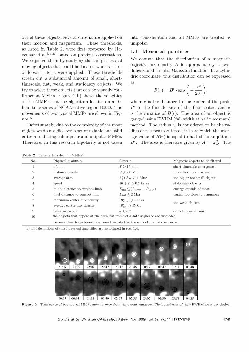
out of these objects, several criteria are applied ontheir motion and magnetism. These thresholds,as listed in Table 2, were first proposed by Ha-genaar et al.[25,27] based on previous observations.We adjusted them by studying the sample pool ofmoving objects that could be located when stricteror looser criteria were applied. These thresholdsscreen out a substantial amount of small, short-timescale, flat, weak, and stationary objects. Wetry to select those objects that can be visually con-firmed as MMFs. Figure 1(b) shows the velocitiesof the MMFs that the algorithm locates on a 10-hour time series of NOAA active region 10330. Themovements of two typical MMFs are shown in Fig-ure 2.

Unfortunately, due to the complexity of the moatregion, we do not discover a set of reliable and solidcriteria to distinguish bipolar and unipolar MMFs.Therefore, in this research bipolarity is not taken

into consideration and all MMFs are treated asunipolar.

1.4 Measured quantities

We assume that the distribution of a magneticobject’s flux density B is approximately a two-dimensional circular Gaussian function. In a cylin-dric coordinate, this distribution can be expressedas

B(r) = Bc · exp(− r2

2σ2

),

where r is the distance to the center of the peak,Bc is the flux density of the flux center, and σ

is the variance of B(r). The area of an object isgauged using FWHM (full width at half maximum)method. The radius ro is considered to be the ra-dius of the peak-centered circle at which the aver-age value of B(r) is equal to half of its amplitudeBc. The area is therefore given by A = πr2

o. The

Table 2 Criteria for selecting MMFsa)

No. Physical quantities Criteria Magnetic objects to be filtered

1 lifetime T � 15 min short-timescale emergences

2 distance traveled S � 2.0 Mm move less than 3 arcsec

3 average area 7 � Aav � 1 Mm2 too big or too small objects

4 speed 10 � V � 0.2 km/s stationary objects

5 initial distance to sunspot limb Dini � (Rmoat − Rspot) emerge outside of moat

6 final distance to sunspot limb Dfnl � 2 Mm vanish too close to penumbra

7 maximum center flux density |Bcmax| � 55 Gs

too weak objects8 average center flux density |Bc

av | � 35 Gs

9 deviation angle θ � 45◦ do not move outward

10 the objects that appear at the first/last frame of a data sequence are discarded,

because their trajectories have been truncated by the ends of the data sequence.

a) The definitions of these physical quantities are introduced in sec. 1.4.

Figure 2 Time series of two typical MMFs moving away from the parent sunspots. The boundaries of their FWHM areas are circled.


radius is related to the variance according to ro =√2ln2 ·σ. The flux of the object, φ(t), is defined as

the integral of B(r) over (0, γro) and we set γ = 2.

φ(t) =∫ 2π

0

∫ γro

0

B(r) · rdrdω

= 2πBc

∫ γro

0

exp(− r2

2σ2

)· rdr

=(

1 − 2−γ2

ln 2

)· (πr2

o) · Bc

≈ 1.3525A · Bc.

Therefore, the flux of a magnetic object can beobtained as the product of the object’s area A andits center flux density Bc as well as a constant scal-ing factor 1.3525. We denote the maximum valueof φ(t) over the object’s lifetime as φ.

The flux of a sunspot, Φspot(t), is measured byintegrating the flux density within the sunspotboundary in each magnetogram frame. Φspot rep-resents its average value. The radius of a sunspot,Rspot, is the average of the semimajor and semimi-nor of its boundary ellipse. The moat radius Rmoat

is defined in a similar way.

The physical quantities in Table 2 are defined asthe following. Lifetime T is the time duration be-tween the first and last appearances of an object.Distance Traveled S is the length of the displace-ment of an object during its lifetime. Average AreaAav is the arithmetic mean of an object’s area A

over its lifetime. Speed V is the distance traveledby an object divided by its lifetime (V = S/T ).The upper limit is set according to the maximumspeed recorded in literature. Initial/Final Distanceto the Sunspot Limb (Dini,Dfnl) is the distance be-tween the location of the first/last appearance ofan object and the sunspot boundary ellipse. Thesetwo criteria are adjusted manually by observingthe magnetogram movies and outlining an ellip-tical zone in which MMFs are active. MaximumCenter Flux Density Bc

max is the maximum valueof an object’s Bc during its lifetime. Average Cen-ter Flux Density Bc

av is the mean of an object’s Bc

within its lifetime. Deviation Angle θ is the anglebetween an object’s displacement and the radialdirection with respect to the sunspot center.

2 Preliminary results

2.1 Statistics

We differentiate MMFs into two categories by theirpolarities:

α-MMF: having the polarity opposite to theparent sunspot,

β-MMF: sharing the parent sunspot’s polarity.The whole MMF population is separated into2×nspot subpopulations. nspot is the total num-ber of sunspots, in our research nspot = 26. TheMMFs in each subset have the same type and par-ent sunspot. A statistical study is performed in theMMF sample pool to reveal the properties of thetwo types of MMFs and their relationship with theparent sunspots.

For each identified MMF, several physical quan-tities (c.f. sec. 1.4) about its motion and magne-tism are computed and cataloged. The value of aphysical quantity measured from a particular MMFis denoted by the symbol Xτ

si. X is the physicalquantity of interest, e.g. speed, flux. The indicesare:

τ is the nominal category specifying the type ofthe MMF, τ ∈ {α, β}.

s is the index of the parent sunspot, s ∈ {1, 2,· · · , nspot}.

i is the index of the MMF, i ∈ {1, 2, · · · ,

N(τ, s)}.N(τ, s) is the total number of type τ MMFs on

sunspot s.So, Xτ

si stands for the value of quantity X mea-sured from type τ MMF number i on sunspots. For each MMF subpopulation, we calculatethe central tendencies of the measured quantities.Since many of these quantities’ frequency distribu-tions are right-skewed and there is a significant di-vergence between median and mean, in many caseswe use median as the central tendency. The disper-sion is measured by interquartile range or standarddeviation.

For all of the type τ MMFs around sunspot s,the median value of their X is:

Xτs = median{Xτ

si}, i = 1, 2, · · · , N(τ, s),

in which τ and s specify the type and sunspot ofthe MMF subpopulation. For instance, φα

s stands


for the median of the maximum fluxes of all theα-MMFs on sunspot s. We denote the sequence ofXτ

s calculated from the type τ subpopulations asXτ .

Xτ = {Xτs }, s = 1, 2, · · · , nspot.

E.g. φα is the sequence of φαs of all the α sub-

populations. We call Xα and Xβ together as thesunspot medians, X = {Xα, Xβ}.

The properties of MMFs of different sunspotsare different. In order to investigate the relation-ship between the sunspots and the characters ofthe subpopulations of MMFs around them, we plotthe sunspot medians (X) of the measured quanti-ties as the functions of the sunspot radii (Rspot) orflux (Φspot). For instance, Figure 3(a) shows T , thesunspot medians of MMFs’ lifetimes, as a functionof Rspot.

The MMF population as a whole can be de-scribed by the frequencies and central tendenciesof the measured quantities. The frequency distri-bution of a quantity can be illustrated by plottinga histogram of the values measured from the en-tire MMF sample pool. For instance, Figure 3(b)shows the frequency distribution of speed V of allidentified α- and β-MMFs. Because the subpopu-lations N(τ, s) of MMFs on different sunspots canbe different by one order of magnitude, the over-all population median or mean of all the Xτ

si inthe sample pool would be heavily biased by thosesunspots that produce more MMFs. In order togive every sunspot equal weight on the overall cen-tral tendency, we define the equal-weight popula-tion average 〈Xτ 〉 of all the type τ MMFs’ X asthe arithmetic mean of the sunspot median valuesXτ .

〈Xτ 〉 = mean{Xτs } s = 1, 2, · · · , nspot.

In this way, a big sunspot that has hundreds ofMMFs would have equal weight on these popula-tion averages as that of a small sunspot which onlyhas dozens of MMFs. In the rest of this paper,we use 〈Xα〉 and 〈Xβ〉 as the central tendency ofthe whole MMF sample pool and refer to them aspopulation averages.

The relationships among MMFs’ physical prop-erties can be studied by multiple regression. For

example, Figure 4 is a scatter diagram of MMFs’initial distances to sunspot (Dini, baseline) againsttheir maximum fluxes (φ, vertical axis).

Figure 3 (a) The sunspot median values of MMF’s lifetime (T )

as a function of sunspot radii. The ordinate of each square/star is

the median value of the lifetimes (T ) of all the α/β-MMFs found

around a particular sunspot, as defined in sec. 2.1. The abscissa

is the radius (Rspot) of the parent sunspots in million meters.

The T of α-MMFs (square) decrease with Rspot, while those of

β-MMFs (star) do not show obvious correlation with Rspot, as

illustrated by the estimated regression lines. The population av-

erage lifetime (〈T 〉, c.f. sec. 3.1) of α/β-MMFs is 1.5/1.7 hours.

In general, β-MMFs live slightly longer than α-MMFs. (b) The

frequency distribution of all identified MMFs’ speeds. The aver-

age value 〈V 〉 is about 0.6 km/s. The threshold value for speed

is set as 0.2 km/s.

2.2 Population and production

MMFs are found around all studied sunspots, in-cluding those not decaying and those not having apenumbra. The MMF production rate (Rprod) ofa sunspot is the number of newly emerged MMFsaround the sunspot per hour, i.e. the total numberof identified MMFs divided by the time duration of


the data sequence. Because criterion No. 10 dis-cards all the MMFs identified in the beginning orat the end of the data set, one median lifetime T τ

s

is subtracted from the divisor. The type ratio,

Figure 4 The scatter plots of the maximum fluxes (φ) of all

the α-MMFs (square) and β-MMFs (star) against their initial

distances to the sunspot limb (Dini). Majority of the MMFs

emerge 0∼5 Mm outside the sunspot limb and have φ smaller

than 10×1018 Mx. Strong α-MMFs usually emerge far from the

sunspots, while most strong β-MMFs emerge close or even inside

the penumbra boundary.

Rtype, is the quotient of the production rateof α-MMFs divided by that of β-MMFs,Rtype=Rα

prod/Rβprod. If a sunspot produces equal

numbers of α- and β-MMFs, then Rtype would be1.

Around the 26 sunspots, the program identifies3675 MMFs, among which the number of α-MMFsis similar to β-MMFs. Rprod varies from 4 to 27 andit increases with the sunspot radius, as shown inFigure 5(a). Large sunspots are more productivein generating MMFs. The four largest sunspotsproduce more α-MMFs than β-MMFs, while the

Rtype of the five smallest sunspots are less than 1.The Rtype of middle-sized sunspots scatters. Forour limited samples of sunspots, Rtype varies withinthe range of 0.2 and 6 and it does not show obviousrelationship with the polarity or evolution phase ofthe parent sunspot.

Figures 4(a) and 4(b) are the scatter plots ofφ versus Dini (MMFs’ initial distances to sunspotlimbs) for the α- and β-MMFs respectively. Mostof the MMFs emerge at 0−5 Mm outside of thesunspot limb. On average, α-MMFs emerge anddisappear farther (4.1/8.3 Mm) away from theparent sunspots than β-MMFs do (2.0/5.5 Mm).There are a certain number of β-MMFs with neg-ative Dini. That is to say they are produced in-side the penumbra boundary[21,23]. Few α-MMFsemerge within the penumbra.

Figure 5 (a) The number of MMFs identified around the

sunspots per hour (Rprod, the MMF production rate) as a func-

tion of the sunspot radius. Rαprod (square) and Rβ

prod (star) in-

crease with Rspot. (b) The sunspot medians of MMFs’ initial

distances to the sunspot limbs (Dini) as functions of Rspot. Dαini

increases with Rspot while the distribution of Dβini is narrower

and almost sunspot-independent. The plot of the MMFs’ final

distances to the sunspots (Dfnl) has a similar pattern.


Figure 5(b) shows the sunspot medians of Dini asa function of Rspot. The plot of the final distancesto sunspots (Dfnl) has a similar pattern. Both Dini

and Dfnl of α-MMFs increase with Rspot. However,those of β-MMFs do not show such a disposition.

2.3 Motion

Most of the MMFs materialize right outside of thepenumbra limb (c.f. Figure 4), then move out-ward roughly along the radial direction (c.f. Fig-ure 1(b)), and at last vanish somewhere within themoat. A small number of them move into the sur-rounding network.

During their whole lifetimes, MMFs move2−12.5 Mm. Figure 6(a) shows the nearly expo-nential frequency distribution of MMFs’ distancetraveled (S). The high skewness (1.64) indicatesthat the S of most MMFs is below the popula-tion mean value (3.7 Mm). Figure 6(a) also sug-gests that numerous objects that move less than2.0 Mm are discarded by the criterion No. 2. Theradial and azimuthal components of MMFs’ dis-placements are also exponentially distributed. Sα

(Sβ) is in the range 2.7–5.9 (2.8–3.6) Mm. On av-erage, MMFs move 3.1 Mm in the radial and 0.8Mm in the azimuthal direction. α-MMFs move alittle further than β-MMFs and their deviation an-gles are approximately 20% larger than those ofβ-MMFs.

Figure 6(b) shows the sunspot medians of the ra-dial distance traveled (Srad) by MMFs as a functionof Rspot. It shows that Sα

rad ranges from 2.5 to 4.5Mm and it decreases with Rspot. The α-MMFs ofsmall sunspots move further in the radial directionthan those of large sunspots. Sβ

rad is distributedwithin a small range (2.5–3.4 Mm) and does notshow obvious correlation with Rspot. In the az-imuthal direction, the distributions of the traveleddistances of both types of MMFs are almost notassociated with Rspot.

Figure 3(b) is a histogram of MMF’s speed. 80%of MMFs move at 0.3−1.0 km/s. The popula-tion average speed 〈V 〉 is about 0.6 km/s. Thefastest ones move at 2.6 km/s. The low-end cutoffis caused by the criterion No. 4. In both radialand azimuthal directions, α-MMFs move about

15% faster than β-MMFs. V ranges within 0.4–0.9 km/s and does not show obvious correlationwith Rspot or developing phase.

Figure 6 (a) The frequency distribution of all identified MMFs’

distance traveled. The nearly-exponential distribution suggests

that the majority of MMFs move a relatively short distance. A

large number of objects that move a distance shorter than 2 Mm

are discarded by our criteria. (b) The sunspot medians of the

MMF’s radial distance traveled (Srad) as a function of Rspot.

Sαrad (square) decrease with Rspot while Sβ

rad (star) only have a

small variation.

On average, the lifetime of α/β-MMFs is ∼1.5/1.7 h. 85% of MMFs live for 0.25−3 h and 2%live longer than 5 h. The longest lifetime of ob-served α/β-MMFs is 8.4/8.2 h. Figure 3(a) showsthat T α range from 1.1 to 3.1 h and decrease withRspot. Small sunspots’ α-MMFs usually move fur-ther than those of big ones (c.f. Figure 6(b)),which is due to their longer liftimes instead of be-ing able to move faster. The range of T β is nar-rower (1.3−2.0 h) and they are almost sunspot-independent.

2.4 Magnetic flux content

MMFs appear in a wide range of sizes and fluxes,


which are associated with MMF’s type, Dini, andΦspot.

The flux of most of the MMFs is smaller than10×1018 Mx. A comparison of Figures 4(a) and4(b) shows that, α-MMFs with φ larger than10×1018 Mx usually emerge far from the sunspots(Dini �5 Mm), while most β-MMFs with largefluxes emerge near the sunspot limbs (Dini �5 Mm).

Figures 7(a) and 7(b) are plots of φα and φβ asfunctions of Φspot. It shows that large sunspots pro-duce MMFs with large flux. This trend is especiallyobvious for α-MMFs. The biggest φα (12.5×1018

Mx) is one order of magnitude larger than thatof the smallest sunspot (1.6×1018 Mx). φβ has asmaller range (4.8∼11.4×1018 Mx) and increaseswith Φspot at a lower rate. For most of the smalland middle-sized sunspots, φβ is generally largerthan φα. These dispositions of φ are further illus-trated by Figure 8(a), a scatter plot of the sunspotmedians of Bc

av (MMFs’ average central flux den-

Figure 7 φα (a) and φβ (b) as functions of the sunspot flux.

φ is MMF’s maximum flux. Error bars show the standard devia-

tions. Large sunspots generate MMFs with large flux, especially

for type α. MMF’s center flux density shows a similar trend (c.f.

Figure 7(a)).

Figure 8 (a) Bcav as a function of Φspot. Bc

av is the average flux

density of MMF’s flux center during the MMF’s lifetime. Gener-

ally Bcav increase with Φspot. For most of the sunspots, Bc

av of

β-MMFs are stronger than those of α-MMFs. (b) The frequency

distribution of all identified MMFs’ average area Aav. The upper

and lower end cut-offs are set by our criterion No. 3. A large

number of small or flat features are discarded.

sity) as a function of Φspot. Bcav, esp. α-MMFs’,

increase with Φspot. For most of the sunspots,β-MMFs’ Bc

av is larger than its α counterpart.The sunspot medians of α-MMFs’ average area

(Aαav) range from 1.1 to 6.6 Mm2 and increase with

Φspot. The range of Aβav is much narrower (1.4–3.6

Mm2) and they do not show correlation with Φspot.The population average value 〈Aav〉 is ∼2.3 Mm2.Figure 8(b) is a frequency histogram of Aav. Itshigh skewness indicates that there should be nu-merous magnetic objects that are smaller than 1Mm2 and are screened by our criterion No. 3.

2.5 Sunspot magnetic flux outflow

The relationships among the sunspots’ magneticflux outflow, flux loss, and developing phases areinvestigated as well.

We calculate the average sunspot flux loss rate


(−d(Φspot(t))/d(t)) using a line-fit routine. We re-gard the flux transport rate as the total flux car-ried away by MMFs per hour. Within the moat re-gion, a thin elliptical loop concentric to the sunspotboundary is set up to count the traversing MMFs.The size and thickness of the loop are optimizedto allow the maximum number of MMFs to crossits inner or outer boarder. The flux transportrate is the total flux of these traversers per hour:|∑cross

φ|.Although our measurements of flux transport

rate (0.2−8.3×1019 Mx·h−1) basically comportswith the range of other observations, they do notshow noticeable correlation with the sunspot fluxloss rates. For some of the sunspots, neither theflux transport rate nor the flux loss rate is consis-tent with the recorded developing phases.

3 Conclusion

We develop a tracking code and use it to pursueMMFs on the magnetogram series of 26 sunspots.A statistical analysis on the kinematic and mag-netic properties of the identified MMFs is carriedout. We find that the statistical characteristic ofa sunspot’s MMF set is relevant to the parentsunspot. In several aspects the two categories ofMMFs have different statistical characteristics.

We find that the sunspots produce 4 to 27MMFs per hour and this production rate tendsto increase with the sunspot radius. Generally,α-MMFs emerge and disappear farther from thesunspot boundary than β-MMFs do. This is espe-cially obvious for MMFs with above-average flux.α-MMF’s initial/final distances to the sunspotlimbs increase with the parent sunspot radius.β-MMFs emerge/vanish at similar distances amongthe sunspots.

The α- and β-MMF subpopulations exhibit awide range of central tendencies. According to thesunspot median values, typical α/β-MMFs emergeat 2.2−8.1/0.1−3.2 Mm outside the penumbralimb. They are 1.1−6.6/1.4−3.6 Mm2 in areaand carry 1.4−12.5/4.8−11.4 ×1018 Mx of flux.They live for 1.1−3.1/1.3−2.0 h, and travel a dis-tance of 2.7−5.9/2.8−3.6 Mm with the speed of0.5−0.9/0.4−0.7 km/s. The frequency distribu-

tions of the MMFs’ distance traveled, flux, andarea are approximately exponential, with most ofvalues below the arithmetic mean.

The sunspot median values of α-MMFs’ distancetraveled and lifetime decrease with the sunspot ra-dius, while those of α-MMFs’ area and flux in-crease with sunspot flux. Compared to α-MMFs ofsmall sunspots, large sunspots tend to produce bigα-MMFs that live shorter, move nearer, and carrymore flux. It is noticed that, in some of the scatterplots, few outliers bias the least squares estima-tion. In our future research, residual analysis willbe performed to construct the confidence intervalsand estimate the regression coefficients properly.

β-MMF’s motion and magnetism have muchweaker correlations with Φspot or Rspotthanα-MMFs do. This might indicate that the gener-ation mechanism of β-MMFs is relatively uniformamong different sunspots, while that of α-MMFs ismore relevant to the structure and surroundings ofthe sunspots. This needs to be further studied inthe scenario of supergranulation[19] and subphoto-spheric convection.

We calculate the sunspots’ magnetic flux outflowtransported by MMFs and the sunspot flux loss,but do not find obvious correlation between them.The nearly exponential distributions of MMF’sarea, distance traveled, and flux are consistent withHagenaar’s observation[27] and suggest that numer-ous small, weak, short-timescale objects fall underour criteria and are not counted. These culls mightconstitute a substantial amount of sunspots’ fluxoutflow. As Vrabec[5] has commented, the mag-netic flux outflow is a “considerably more compli-cated process than” fragmentation of sunspots intoMMFs. Further investigations using higher resolu-tion data and estimation methods need to be car-ried out to estimate the flux outflow.

We plan to examine a larger sample of sunspotsto investigate the relationship between the char-acteristics of MMFs and the parent sunspot morethoroughly. We also intend to continue this studyon higher resolution data, and discuss MMFs’ evo-lution and physical structure.

The authors would like to thank Jiangtao Su, Haiqing Xu,

Yu Gao, and H. J. Hagenaar for reading and commenting


on the manuscript. Thanks are also due to the referees

for their comments and suggestions on how to improve the

manuscript. This research has made use of Interactive Data

Language, SolarSoft[31], SAOImage DS9[32], Linff[33] and MDI

High-Resolution Data Catalog. SOHO is a project of interna-

tional collaboration between ESA and NASA.

1 Sheeley N R Jr. The evolution of the photospheric network.

Sol Phys, 1969, 9: 347–357

2 Vrabec D. Magnetic fields spectroheliograms from the San Fer-

nando observatory. In: Howard R, ed. Sol Magn Fields, IAU

Symposium, 1971, 43: 329–339

3 Harvey K, Harvey J. Observations of moving magnetic features

near sunspots. Sol Phys, 1973, 28: 61–71

4 Shine R, Title A. Sunspots: Moving magnetic features and

moat flow. In: Murdin P, ed. Encyclopedia of Astronomy and

Astrophysics, 2001

5 Vrabec D. Streaming magnetic features near sunspots. In:

Athay R G, ed. Chromospheric Fine Structure, IAU Sympo-

sium, 1974, 56: 201–231

6 Bernasconi P N, Rust D M, Georgoulis M K, et al. Moving

dipolar features in an emerging flux region. Sol Phys, 2002,

209: 119–139

7 Zhang J, Solanki S K, Woch J. Discovery of inward moving

magnetic enhancements in sunspot penumbrae. Astron Astro-

phys, 2007, 475: 695–700

8 Wilson P R. The cooling of a sunspot. III: Recent observa-

tions. Sol Phys, 1973, 32: 435–439

9 Wilson P R. The generation of magnetic fields in photospheric

layers. Sol Phys, 1986, 106: 1–28

10 Spruit H C, Title A M, van Ballegooijen A A. The generation

of magnetic fields in photospheric layers. Sol Phys, 1987, 110:

115–128

11 Lee J W. Observational evidence for various models of moving

magnetic features. Sol Phys, 1992, 139: 267–273

12 Penn M J, Kuhn J R. Imaging spectropolarimetry of the He I

1083 nanometer line in a flaring solar active region. Astrophys

J, 1995, 441: L51–L54

13 Yurchyshyn V B, Wang H, Goode P R. On the correlation

between the orientation of moving magnetic features and the

large-scale twist of sunspots. Astrophys J, 2001, 550: 470–474

14 Zhang J, Solanki S K, Wang J. On the nature of moving mag-

netic feature pairs around sunspots. Astron Astrophys, 2003,

399: 755–761

15 Choudhary D P, Balasubramaniam K S. Multiheight prop-

erties of moving magnetic features. Astrophys J, 2007, 664:

1228–1233

16 Kubo M, Shimizu T, Tsuneta S. Vector magnetic fields of mov-

ing magnetic features and flux removal from a sunspot. As-

trophys J, 2007, 659: 812–828

17 Ryutova M, Hagenaar H. Magnetic solitons: Unified mecha-

nism for moving magnetic features. Sol Phys, 2007, 246: 281–

294

18 Brickhouse N S, Labonte B J. Mass and energy flow near

sunspots. I - observations of moat properties. Sol Phys, 1988,

115: 43–60

19 Wang H. On the relationship between magnetic fields and su-

pergranule velocity fields. Sol Phys, 1988, 117: 343–358

20 Zhang H, Ai G, Wang H, et al. Evolution of magnetic fields

and mass flow in a decaying active region. Sol Phys, 1992, 140:

307–316

21 Sainz Dalda A, Martınez Pillet V. Moving magnetic features

as prolongation of penumbral filaments. Astrophys J, 2005,

632: 1176–1183

22 Li X, Zhang J, Wang J. Unipolar moving magnetic features:

An observation. In: Bothmer V, Hady A A, eds. Solar Ac-

tivity and its Magnetic Origin, IAU Symposium, 2006, 233:

83–84

23 Ravindra B. Moving magnetic features in and out of penum-

bral filaments. Sol Phys, 2006, 237: 297–319

24 Brooks D H, Kurokawa H, Berger T E. An Hα surge provoked

by moving magnetic features near an emerging flux region.

Astrophys J, 2007, 656: 1197–1207

25 Hagenaar H J, Schrijver C J, Title A M, et al. Dispersal of

magnetic flux in the quiet solar photosphere. Astrophys J,

1999, 511: 932–944

26 Fletcher L, Pollock J A, Potts H E. Tracking of TRACE ul-

traviolet flare footpoints. Sol Phys, 2004, 222: 279–298

27 Hagenaar H J, Shine R A. Moving magnetic features around

sunspots. Astrophys J, 2005, 635: 659–669

28 DeForest C E, Hagenaar H J, Lamb D A, et al. Solar magnetic

tracking. I. Software comparison and recommended practices.

Astrophys J, 2007, 666: 576–587

29 Lamb D A, DeForest C E, Hagenaar H J, et al. Solar magnetic

tracking. II. The apparent unipolar origin of quiet-sun flux.

Astrophys J, 2008, 674: 520–529

30 Scherrer P H, Bogart R S, Bush R I, et al. The solar oscilla-

tions investigation - michelson doppler imager. Sol Phys, 1995,

162: 129–188

31 Freeland S L, Handy B N. Data analysis with the solarSoft

system. Sol Phys, 1998, 182: 497–500

32 Joye W A. New features of SAOImage DS9. In: Gabriel C,

Arviset C, Ponz D, et al., eds. Astronomical Data Analysis

Software and Systems XV, ASP Conference Series, 2006, 351:

574–576

33 Wiegelmann T, Inhester B, Lagg A, et al. How to use mag-

netic field information for coronal loop identification. Sol Phys,

2005, 228: 67–78

34 Gallagher P T, Moon Y J, Wang H. Active-region monitoring

and flare forecasting I. Data processing and first results. Sol

Phys, 2002, 209: 171–183


tracking moving magnetic features in the photosphere · phys.scichina.com tracking moving magnetic...

Documents