Tracking a Minimum Bounding Rectangle based onExtreme Value Theory

Marcus Baum and Uwe D. Hanebeck

Abstract— In this paper, a novel Bayesian estimator for theminimum bounding axis-aligned rectangle of a point set basedon noisy measurements is derived. Each given measurementstems from an unknown point and is corrupted with additiveGaussian noise. Extreme value theory is applied in order toderive a linear measurement equation for the problem. Thenew estimator is applied to the problem of group target andextended object tracking. Instead of estimating each singlegroup member or point feature explicitly, the basic idea is totrack a summarizing shape, namely the minimum boundingrectangle, of the group. Simulation results demonstrate thefeasibility of the estimator.

I. INTRODUCTION

Minimum bounding rectangles are frequently used inmany application areas like image processing, geography,and tracking. This paper is concerned with the problem ofestimating the minimum bounding axis-aligned rectangle ofa set of points. However, the points, which we also call mea-surement sources, are not given directly. Only measurementscorrupted with Gaussian noise are available. Furthermore, itis not known from which measurement source a particularmeasurement stems.

The contributions of the paper are the following: Wederive a novel recursive Bayesian estimator [1] for the min-imum axis-aligned bounding rectangle given noisy positionmeasurements. In order to derive the estimator, we employtechniques from extreme value theory, which deals with theprobability of the minimum or maximum of random experi-ments. The resulting measurement equation is linear, so thatthe well-known Kalman filter can be used for inference.

Finally, we apply the proposed estimator to the problem oftracking a group of point targets [2] (see Fig. 1). The basicapproach followed here is to track the minimum boundingrectangle of the group, instead of each single group member.This is suitable in cases where data association is too difficultor one is simply not interested in the exact position of theindividual group members. For example, data associationmay become hard, when the group members are closelyspaced, i.e., their validation gates overlap. For a large numberof targets, e.g., more than 10, data association algorithmsthen may even become computationally intractable.

A similar problem occurs when tracking an extendedtarget object, where several point features, i.e., measurementsources, on the target surface may cause measurements. Inthis case, the proposed method can be used to track the

M. Baum and U. D. Hanebeck are with the Intelligent Sensor-Actuator-Systems Laboratory (ISAS), Institute for Anthropomatics, Karlsruhe In-stitute of Technology (KIT), Germany. marcus.baum@kit.edu,uwe.hanebeck@ieee.org

= Measurement source

= Measurement

Fig. 1: Extended object and group of targets.

minimum bounding rectangle of the shape of the extendedobject. Such tracking problems arise for instance in airsurveillance, where aircraft are tracked with high-resolutionradar devices (see Fig. 1). The estimator proposed in thispaper is suitable if the minimum bounding rectangle of themeasurement sources coincides with the minimum boundingrectangle of the target (see Fig. 1). It is important to notethat the application area for summarizing shape estimation intracking is different from Spatial Distribution Models [3] orRandom Hypersurface Models [4]. These models are suitablefor a rather diffuse measurement generation process, e.g.,scenarios with low detection probability, partly unresolvedtargets, and high measurement noise.

The remainder of this paper is structured as follows:After a brief overview of related methods in Section II,we give a detailed problem formulation in Section III.Then, we introduce some basic results from extreme valuetheory (see Section IV), which are employed for derivingthe novel estimator for the minimum bounding rectangle(see Section V). The proposed estimator is then evaluatedin Section VI. Finally, conclusions and an outlook to futurework are given in Section VII.

II. RELATED WORK

In this section, we give a short overview of related methodsto the considered problem. Because the measurement sourcesfor which the smallest enclosing rectangle is to be estimatedare unkwown (and should not be estimated explicitely), it isnecassary to make proper (implicit) assumptions on the loca-tion of the measurement sources. One statistical approach forthe problem of estimating rectangles is to assume that eachmeasurement source is an independent random draw from auniform distribution on the true rectangle. Such a distributionis also called spatial distribution [3], [5]. This approach suf-fers from the disadvantage that in real-world applications, themeasurement sources are in fact not uniformly distributed onthe rectangle. Then, a spatial distribution model may providepoor estimation results. Furthermore, there are no closed-form expressions for a Bayesian solution with a uniformspatial distribution on a rectangle available. Non-Bayesian

Measurementsource model

Measurement model

Stochastic noise wk

(a) Independent generation of each single measurement source. Examples:Random Hypersurface Models, Spatial Distribution Models.

Measurementsource model

Measurement model

Stochastic noise wk

(b) Batch generation of all measurement sources. The true shape is thesmallest enclosing shape of the measurement sources.

= Measurement source = Measurement = True Shape

Fig. 2: Different models for generating measurement sourcesat a particular time step.

solutions to this problems have also been considered in acontext different from tracking, for instance in [6].

In [4], so-called Random Hypersurface Models are intro-duced for the purpose of tracking extended targets. This ap-proach assumes that each measurement source is an elementof a hypersurface generated from a random draw of a one-dimensional probability distribution. In fact, this approachcould also be used to model a rectangle. However, also aRandom Hypersurface Model imposes statistical assumptionson the measurement sources and no closed-form expressionsare currently available for rectangles.

A further related approach for tracking rectangular-shapedextended target objects was introduced in [7]. There, it isonly assumed that the measurement sources lie on the targetsurface. No (statistical) assumptions about the measurementsources are made. If there is no measurement noise, the prob-lem can be formulated as a set-theoretic estimation problem.Stochastic measurement noise then requires a combined set-theoretic and stochastic estimator. With this approach it isnot possible to estimate the size of the target extent onlywith position measurements. In [7], it is necessary to assumethat the number of measurements, which are received at aparticular time step depends on the size of the extendedobject in order to estimate the size of minimum boundingrectangle. This is a quite restrictive assumption, which,however, is often fulfilled in target tracking applications.The approach presented in this paper does not have thisrestriction.

Apart from the above approaches, which implicitly modelmeasurement sources, there also exist approaches that ex-plicitly model each single measurement sources on the targetextent [8], [9], [10]. These approaches require data associ-ation and are thus computationally expensive. Furthermore,they require dynamic models for the measurement sources,which may not be available.

III. PROBLEM FORMULATION

We treat the problem of tracking the parameters of theaxis-aligned minimum bounding rectangle of a finite set of

N -dimensional points based on measurements corrupted withadditive Gaussian noise. At each time step k, a finite setof measurements Zk := {zk,l}

nk

l=1 becomes available. Eachindividual measurement zk,l ∈ IRN is the noisy observationof a point zk,l ∈ IRN , named measurement source, i.e.,

zk,l = zk,l + wk,l , (1)

where wk,l denotes additive white Gaussian noise1 withdiagonal covariance matrix diag([σ1, . . . , σN ]). The locationof the measurement source zk,l is totally unknown. The goalis to estimate the parameters of the axis-aligned minimumbounding rectangle of {zk,l}

nk

l=1.Since we focus on tracking applications, the parameters

of the minimum bounding rectangle may evolve over time.Its temporal evolution is modeled by means of a stochasticmotion model. Note that no dynamic models for the mea-surement sources itself are given.

In this paper, we seek a Bayesian estimator [1] for theminimum bounding rectangle, which is a recursive updatescheme for a probability distribution over the unknown stateaccording to Bayes’ rule .

REMARK 1 The above problem formulation is different fromSpatial Distribution Models [3] and Random HypersurfaceModels [4], which were introduced in the context of extendedobject tracking. There, each single measurement source isgenerated independently according to a stochastic process.As a consequence, these models allow for receiving a singlemeasurement at a particular time step from an extendedobject. Here, a single measurement per time step wouldimmediately yield a point since the minimum boundingrectangle of a point is a point. These two different generativemodels for the measurements are illustrated in Fig. 2.

REMARK 2 The above problem is fundamentally differentfrom statistical shape fitting [11], [12], [13]. In statisticalshape fitting, one deals with estimating a shape, like a circle,from given noisy measurements. However, the big differenceis that in shape fitting, the measurement sources all stem fromthe border of the shape. Here, the measurement sources mayalso lie in the inner of the shape, i.e., the rectangle.

IV. EXTREME VALUE THEORYIn this section, a brief introduction to extreme value theory

is given. Extreme value theory [14] is a branch of statisticsthat deals with extreme values such as minima and maximaof random experiments. The application area of extremevalue theory is quite broad. Just to mention a few, it hasbeen applied for (financial) risk management [15], floodprediction, engineering and, insurance assessment [16].

In probability theory, the Central Limit Theorem states thatthe mean of a sequence of independent identically distributedrandom variables approaches a normal distribution (undercertain assumptions). Similarly, it can be shown that theextreme value of a sequence of independent identically dis-tributed random variables approaches a limiting distribution.

1All random variables are printed bold face in this paper.

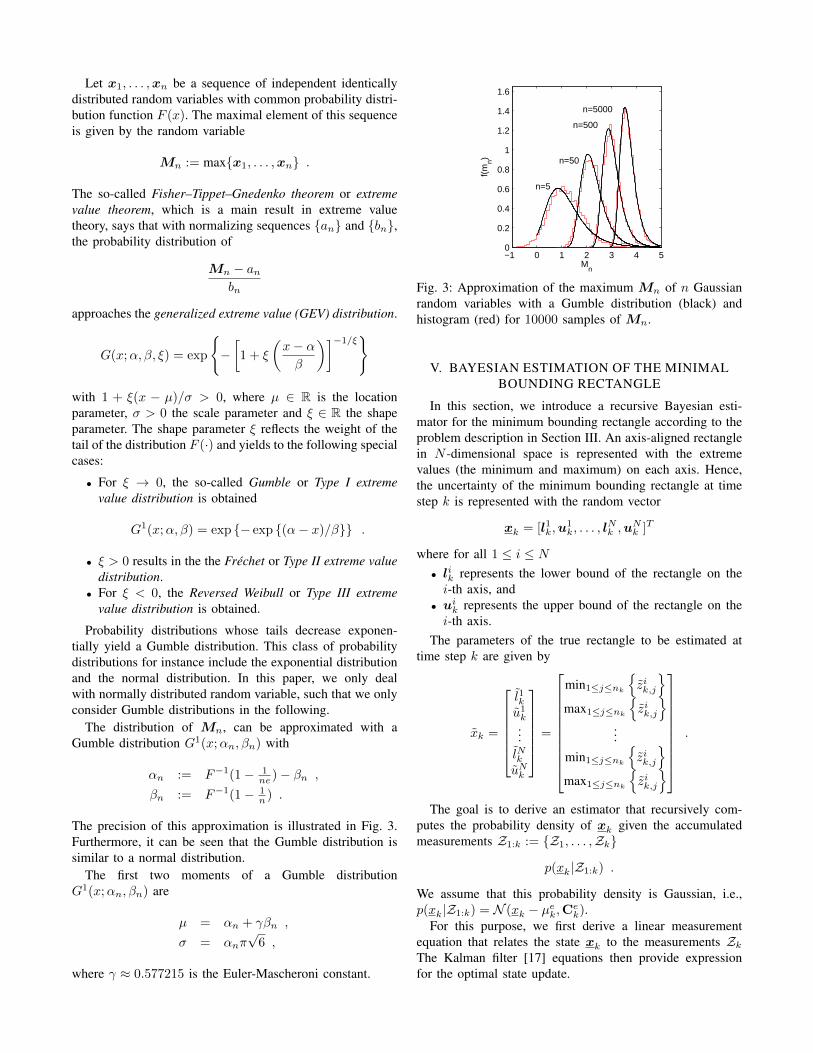
Let x1, . . . ,xn be a sequence of independent identicallydistributed random variables with common probability distri-bution function F (x). The maximal element of this sequenceis given by the random variable

Mn := max{x1, . . . ,xn} .

The so-called Fisher–Tippet–Gnedenko theorem or extremevalue theorem, which is a main result in extreme valuetheory, says that with normalizing sequences {an} and {bn},the probability distribution of

Mn − anbn

approaches the generalized extreme value (GEV) distribution.

G(x;α, β, ξ) = exp

{−[1 + ξ

(x− αβ

)]−1/ξ}

with 1 + ξ(x − µ)/σ > 0, where µ ∈ R is the locationparameter, σ > 0 the scale parameter and ξ ∈ R the shapeparameter. The shape parameter ξ reflects the weight of thetail of the distribution F (·) and yields to the following specialcases:

• For ξ → 0, the so-called Gumble or Type I extremevalue distribution is obtained

G1(x;α, β) = exp {− exp {(α− x)/β}} .

• ξ > 0 results in the the Frechet or Type II extreme valuedistribution.

• For ξ < 0, the Reversed Weibull or Type III extremevalue distribution is obtained.

Probability distributions whose tails decrease exponen-tially yield a Gumble distribution. This class of probabilitydistributions for instance include the exponential distributionand the normal distribution. In this paper, we only dealwith normally distributed random variable, such that we onlyconsider Gumble distributions in the following.

The distribution of Mn, can be approximated with aGumble distribution G1(x;αn, βn) with

αn := F−1(1− 1ne )− βn ,

βn := F−1(1− 1n ) .

The precision of this approximation is illustrated in Fig. 3.Furthermore, it can be seen that the Gumble distribution issimilar to a normal distribution.

The first two moments of a Gumble distributionG1(x;αn, βn) are

µ = αn + γβn ,

σ = αnπ√

6 ,

where γ ≈ 0.577215 is the Euler-Mascheroni constant.

−1 0 1 2 3 4 50

0.2

0.4

0.6

0.8

1

1.2

1.4

1.6

n=5

n=50

n=500

n=5000

Mn

f(m

n)

Fig. 3: Approximation of the maximum Mn of n Gaussianrandom variables with a Gumble distribution (black) andhistogram (red) for 10000 samples of Mn.

V. BAYESIAN ESTIMATION OF THE MINIMALBOUNDING RECTANGLE

In this section, we introduce a recursive Bayesian esti-mator for the minimum bounding rectangle according to theproblem description in Section III. An axis-aligned rectanglein N -dimensional space is represented with the extremevalues (the minimum and maximum) on each axis. Hence,the uncertainty of the minimum bounding rectangle at timestep k is represented with the random vector

xk = [l1k,u1k, . . . , l

Nk ,u

Nk ]T

where for all 1 ≤ i ≤ N• lik represents the lower bound of the rectangle on thei-th axis, and

• uik represents the upper bound of the rectangle on thei-th axis.

The parameters of the true rectangle to be estimated attime step k are given by

xk =

l1ku1k...lNkuNk

=

min1≤j≤nk

{zik,j

}max1≤j≤nk

{zik,j

}...

min1≤j≤nk

{zik,j

}max1≤j≤nk

{zik,j

}

.

The goal is to derive an estimator that recursively com-putes the probability density of xk given the accumulatedmeasurements Z1:k := {Z1, . . . ,Zk}

p(xk|Z1:k) .

We assume that this probability density is Gaussian, i.e.,p(xk|Z1:k) = N (xk − µek,Ce

k).For this purpose, we first derive a linear measurement

equation that relates the state xk to the measurements ZkThe Kalman filter [17] equations then provide expressionfor the optimal state update.

A. Derivation of the Measurement Equation

First, we restrict to a particular axis i and the upper bounduik of the minimum bounding rectangle. In order to estimateuik, we first make the following decisive assumption: The i-thcoordinate of a subset of the measurement sources coincideswith uik, i.e.,

zik,j = uxk for all j ∈ Bu,ik ,

where Bu,ik is a set of indices of measurements. The othermeasurement sources are assumed to be far away from uik sothat they do not influence the maximum distribution. Then,obviously, the following holds:

uik = maxi∈Bu,ik

{zik}.

If the number of elements |Bu,ik | in Bu,ik is known, a Bayesian

estimator for lxk can be derived. Because of the aboveassumption zik,j are independently identically-distributed forj ∈ Bu,ik . Hence, the probability distribution of

maxj∈Bu,ik

{zik,j

}− uik := wi,u

k (2)

is approximately Gumble distributed G1(x; au,ik , bu,ik ) with

au,ik := Φ−1(1− 1

|Bu,ik |e)− bu,ik

bu,ik := Φ−1(1− 1

|Bu,ik |)

where |Bu,ik | denotes the number of elements in Bu,ik and Φ−1

is the inverse cumulative distribution function of a Gaussiandistribution with zero mean and variance σi.

According to Section IV, the Gumble distribution canbe approximated with a Gaussian distribution by means ofanalytic moment matching. A reformulation of (2) yields thelinear measurement equation

uik = uik + wu,ik ,

where wu,ik is approximated with a Gaussian with mean

au,ik + γbu,ik and variance au,ik π√

6 and virtual measurement

uik := max0≤j≤nk

{zik,j

}.

Unfortunately, the number of elements in Bu,ik is unknown.We therefore propose a simple but effective heuristic todetermine it:

Let ru,ik be the number of measurements zk,u with zik,j >uxk . Then, the discrete random variable ru,ik is Binomialdistributed according to

p(ru,ik = r) =

(|Bu,ik |r

)0.5r .

The expectation of ru,ik is E[ru,ik

]= 0.5 · |Bu,ik |. Hence, a

proper approximation for |Bu,ik | is given by

|Bu,ik | ≈ 2 · ru,ikwhere ru,ik := |{j|zik,j > uik}| and uik is the current estimatefor uik . The estimate for |Bu,ik | can also be averaged over

several time steps in order to obtain more robust values.However, then temporal changes of |Bu,ik | are followedslower. For small |Bu,ik |, i.e., |Bu,ik | < 4, it is important that|Bu,ik | is estimated precisely. However, with an increasing|Bu,ik |, it becomes less and less important to estimate |Bu,ik |precisely. This results from the fact that the maximumapproaches the limiting distribution quite fast (see Fig. 3).

In the same manner as for the upper bound uik, a Bayesianestimator can be constructed for the lower bound lik. Withthe pseudo measurement

uik := min0≤j≤nk

{zik,j

},

the measurement equation becomes

lik = lik + wl,ik ,

where wl,ik is approximated with a Gaussian distribution with

mean −(aik + γbik) and variance al,ik π√

6.Finally, we have to compose the above measurement

equations to a single measurement equation for all axes andextreme values. Since the measurement noise on differentaxes is uncorrelated, we obtain

yk

= xk + wk (3)

with measurement

yk

:=[l1k, u

1k, · · · , lNk , uNk

]Tand Gaussian noise term

wk =[wl,1k ,wl,1

k , · · · ,wl,Nk ,wl,N

k ,]

with mean

µwk =

−(a1k + γb1k)a1k + γb1k

...−(aNk + γbNk )aNk + γbNk

and covariance matrix

Cwk = π

√6 · diag([b1k, b

1k, . . . , b

Nk , b

Nk ]) .

One underlying assumption of the above measurementequation is that the minimum and maximum on a particularaxis are independent. This assumption is fulfilled if themeasurement noise is not greater than the width of therectangle. However, we observed that even if this is not thecase, the correlation between the maximum and minimumdistribution is negligible.

B. Measurement Update Step

If the predicted probability density for the parameters attime step k is Gaussian, i.e.,

p(xk|Z1:k−1) = N (xk − µpk,C

pk) ,

the updated estimate p(xk|Z1:k) according to measurementmodel (3) is also Gaussian with mean µek and covariance Ce

k

and results from the Kalman filter equations

µek = µpk + Kk(yk− µpk) ,

Cek = (I−Kk)Cp

k ,

with Kalman gain

Kk = Cpk(Cp

k + Cvk)−1 .

C. Prediction Step

The parameter vector xk of the rectangle is assumed toevolve according to a known Markov model characterized bythe conditional density function p(xk|xk−1). Thus, the pre-dicted probability density at time step k, i.e., p(xk|Z1:k−1),results from the Chapman-Kolmogorov equation

p(xk|Z1:k−1) =

∫p(xk|xk−1)p(xk−1|Z1:k−1)dxk−1 .

If p(xk−1|Z1:k−1) is Gaussian and a linear system equation

xk = Bkxk−1 + vk ,

with white Gaussian noise vk is given, the predictionp(xk|Z1:k−1) is also Gaussian. Its mean µpk and covariancematrix Cp

k can be computed with the formulas of the Kalmanfilter prediction step

µpk = Bkµek−1 ,

Cpk = BT

kCek−1Bk + Cv

k−1 .

VI. EVALUATION

A. Fixed Set of Measurement Sources

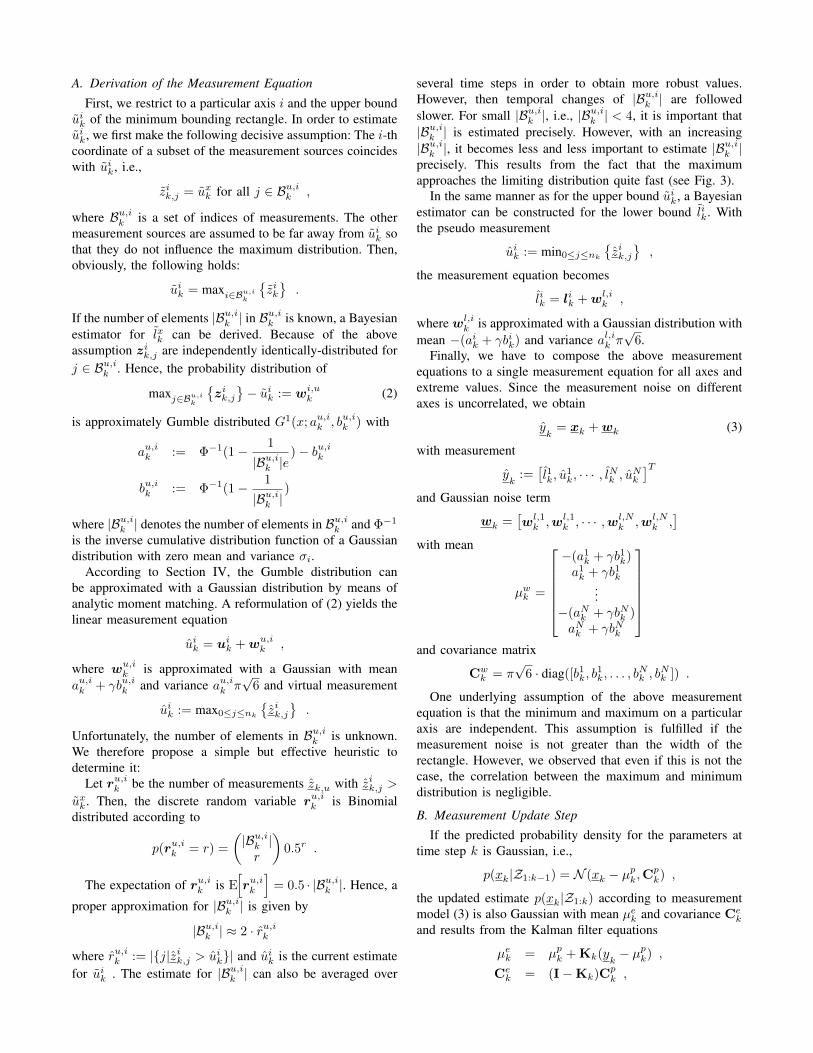
The first example shows the applicability of the presentedestimator for estimating the minimum bounding box. Forthis purpose, a fixed set of measurement sources are ar-ranged in a plane. At each time step, noisy measurementsare received from all measurement sources. The Gaussianmeasurement noise has covariance matrix of diag([1, 1]). Theprior for the rectangle parameters are given by a Gaussiandistribution with mean [−1, 9, 0, 9]T and covariance matrixdiag(4, 4, 4, 4). The estimation results for three differents setsof measurement sources are depicted in Fig. 4.

The estimation results are compared with a spatial distri-bution model [3], [5] that assumes the measurement sourcesto be uniformly distributed on the entire rectangle surface.This spatial distribution model leads to the measurementlikelihood function

p(zk,l|xk) :=1

R(xk)

∫R(xk)

N (z − zk,l,Cvk)dz ,

where R(xk) denotes the area of the rectangle specifiedby the parameter vector xk. As no closed-form expressionsfor the measurement update with this likelihood exists, weapplied the Gaussian Particle Filter [18] for state estimation.Actually, the new approach is computationally far mor attrac-tive than the spatial distribution model, as the new approachresults in a linear formulation of the problem. The spatialdistribution model is not suitable for higher dimensions.

The depicted results in Fig. 4 are chosen such that theestimation results have been converged, i.e., the results do notchange anymore in the subsequent time steps. The differentestimation results of the two estimators result from the differ-ent assumptions on the measurement sources. As the receivedmeasurement only stem from a finite set of measurement

sources, the assumption made by the spatial distributionmodel is not proper. However, the assumptions made by thenew approach appear to justified in this examples.

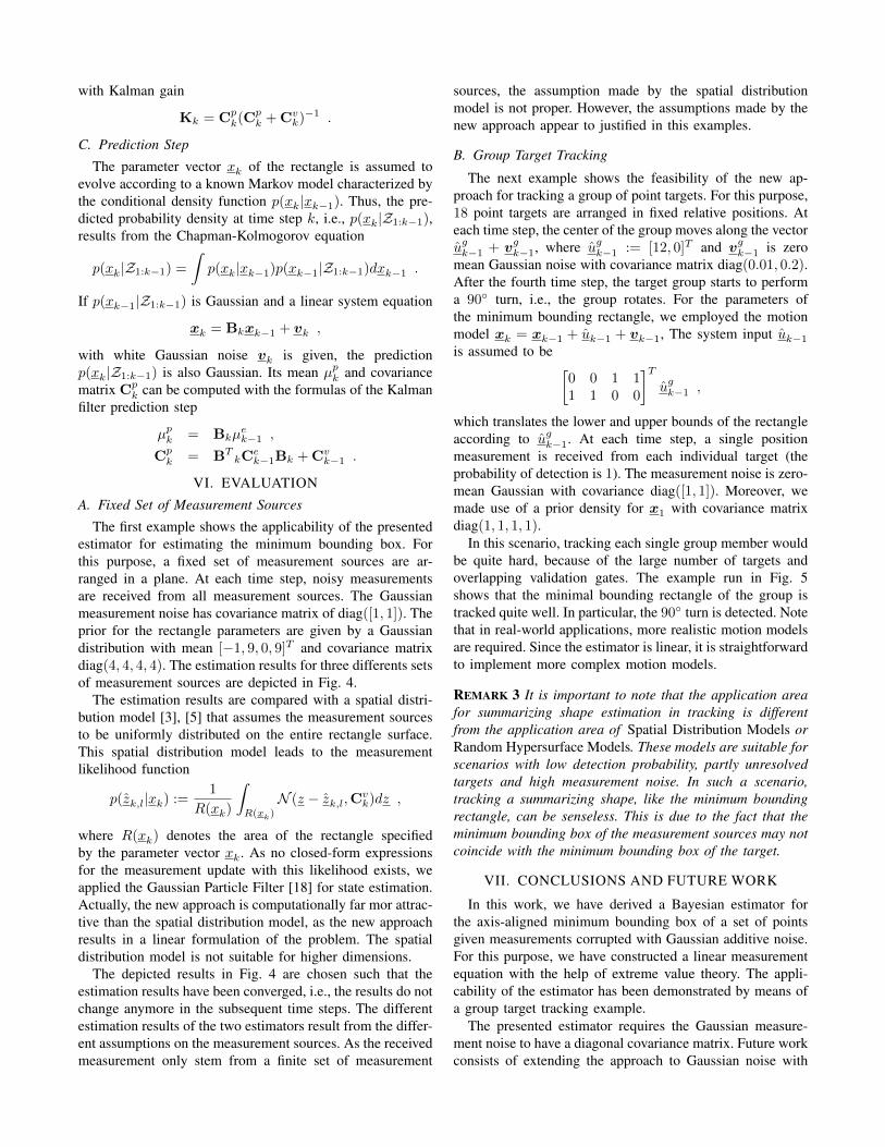
B. Group Target Tracking

The next example shows the feasibility of the new ap-proach for tracking a group of point targets. For this purpose,18 point targets are arranged in fixed relative positions. Ateach time step, the center of the group moves along the vectorugk−1 + vgk−1, where ugk−1 := [12, 0]T and vgk−1 is zeromean Gaussian noise with covariance matrix diag(0.01, 0.2).After the fourth time step, the target group starts to performa 90◦ turn, i.e., the group rotates. For the parameters ofthe minimum bounding rectangle, we employed the motionmodel xk = xk−1 + uk−1 + vk−1, The system input uk−1is assumed to be [

0 0 1 11 1 0 0

]Tugk−1 ,

which translates the lower and upper bounds of the rectangleaccording to ugk−1. At each time step, a single positionmeasurement is received from each individual target (theprobability of detection is 1). The measurement noise is zero-mean Gaussian with covariance diag([1, 1]). Moreover, wemade use of a prior density for x1 with covariance matrixdiag(1, 1, 1, 1).

In this scenario, tracking each single group member wouldbe quite hard, because of the large number of targets andoverlapping validation gates. The example run in Fig. 5shows that the minimal bounding rectangle of the group istracked quite well. In particular, the 90◦ turn is detected. Notethat in real-world applications, more realistic motion modelsare required. Since the estimator is linear, it is straightforwardto implement more complex motion models.

REMARK 3 It is important to note that the application areafor summarizing shape estimation in tracking is differentfrom the application area of Spatial Distribution Models orRandom Hypersurface Models. These models are suitable forscenarios with low detection probability, partly unresolvedtargets and high measurement noise. In such a scenario,tracking a summarizing shape, like the minimum boundingrectangle, can be senseless. This is due to the fact that theminimum bounding box of the measurement sources may notcoincide with the minimum bounding box of the target.

VII. CONCLUSIONS AND FUTURE WORK

In this work, we have derived a Bayesian estimator forthe axis-aligned minimum bounding box of a set of pointsgiven measurements corrupted with Gaussian additive noise.For this purpose, we have constructed a linear measurementequation with the help of extreme value theory. The appli-cability of the estimator has been demonstrated by means ofa group target tracking example.

The presented estimator requires the Gaussian measure-ment noise to have a diagonal covariance matrix. Future workconsists of extending the approach to Gaussian noise with

0 5 10

−2

0

2

4

6

8

10

12

x

y

(a) Time step k = 10.

0 5 10

−2

0

2

4

6

8

10

12

x

y

(b) Time step k = 4.

0 5 10

−2

0

2

4

6

8

10

12

x

y

(c) Time step k = 4.

Fig. 4: Example: Estimating the minimum bounding rectangle of a fixed set of measurement sources. Measurement sources(red dots) and measurements (blue crosses). The results of the novel estimator is given by the black rectangle, the dashedrectangle is the estimation results for the spatial distribution model. The prior for the rectangle parameters is given by aGaussian distribution with mean [−1, 9, 0, 9]T and covariance matrix diag(4, 4, 4, 4).

0 20 40 60 80 100 120 140 160

0

10

20

x

y

Fig. 5: Tracking a group of point targets: Point targets (red dots), measurements (crosses), and estimated ellipse (red) plottedfor several time steps.

non-diagonal covariance matrix. Finally, it will be investi-gated whether the approach can be extended to other shapes,such as arbitrary oriented rectangles, circles or ellipses.Especially for tracking applications, information about thetarget orientation is important.

REFERENCES

[1] D. Hall and J. Llinas, Handbook of Multisensor Data Fusion. CRCPress, May 2001.

[2] M. J. Waxman and O. E. Drummond, “A Bibliography of Cluster(Group) Tracking,” Signal and Data Processing of Small Targets 2004,vol. 5428, no. 1, pp. 551–560, 2004.

[3] K. Gilholm and D. Salmond, “Spatial Distribution Model for TrackingExtended Objects,” Radar, Sonar and Navigation, IEE Proceedings,vol. 152, no. 5, pp. 364–371, October 2005.

[4] M. Baum and U. D. Hanebeck, “Random Hypersurface Models forExtended Object Tracking,” in Proceedings of the 9th IEEE Interna-tional Symposium on Signal Processing and Information Technology(ISSPIT 2009), Ajman, United Arab Emirates, Dec. 2009.

[5] K. Gilholm, S. Godsill, S. Maskell, and D. Salmond, “Poisson Modelsfor Extended Target and Group Tracking,” in SPIE: Signal and DataProcessing of Small Targets, 2005.

[6] M. Bensic and K. Sabo, “Border Estimation of a Two-DimensionalUniform Distribution if Data are Measured with Additive Error,”Statistics - A Journal of Theoretical and Applied Statistics, vol. 41,pp. 311–319(9), August 2007.

[7] M. Baum and U. D. Hanebeck, “Tracking an Extended Object Mod-eled as an Axis-Aligned Rectangle,” in 4th German Workshop onSensor Data Fusion: Trends, Solutions, Applications (SDF 2009),Lubeck, Germany, October 2009.

[8] J. Vermaak, N. Ikoma, and S. Godsill, “Extended object tracking usingparticle techniques,” Aerospace Conference, 2004. Proceedings. 2004IEEE, vol. 3, pp. –1885 Vol.3, March 2004.

[9] ——, “Sequential Monte Carlo Framework for Extended ObjectTracking,” IEE Proceedings on Radar, Sonar and Navigation, vol.152, no. 5, pp. 353 – 363, October 2005.

[10] N. Ikoma and S. Godsill, “Extended Object Tracking with UnknownAssociation, Missing Observations, and Clutter using Particle Filters,”in IEEE Workshop on Statistical Signal Processing, 2003, pp. 502 –505.

[11] Z. Zhang, “Parameter Estimation Techniques: A Tutorial with Appli-cation to Conic Fitting,” Image and Vision Computing, vol. 15, no. 1,pp. 59 – 76, 1997.

[12] J. Porrill, “Fitting Ellipses and Predicting Confidence Envelopes usinga Bias Corrected Kalman filter,” Image Vision Comput., vol. 8, no. 1,pp. 37–41, 1990.

[13] T. Ellis, A. Abbood, and B. Brillault, “Ellipse detection and matchingwith uncertainty,” Image Vision Comput., vol. 10, no. 5, pp. 271–276,1992.

[14] L. de Haan and A. Ferreira, Extreme Value Theory - An Introduction.Springer Verlag, 2006.

[15] P. Embrechts, “Extreme Value Theory: Potential And Limitations AsAn Integrated Risk Management Tool,” Derivatives Use, Trading &Regulation, vol. 6, 2000.

[16] P. Embrechts, T. Mikosch, and C. Kluppelberg, Modelling ExtremalEvents: For Insurance and Finance. London, UK: Springer, 1997.

[17] D. Simon, Optimal State Estimation: Kalman, H Infinity, and Nonlin-ear Approaches, 1st ed. Wiley & Sons, August 2006.

[18] J. Kotecha and P. Djuric, “Gaussian Particle Filtering,” IEEE Trans-actions on Signal Processing, vol. 51, no. 10, pp. 2592 – 2601, Oct.2003.