trace-penalty minimization for large-scale eigenspace...

Trace-Penalty Minimization forLarge-scale Eigenspace Computation

Yin Zhang

Department of Computational and Applied MathematicsRice University, Houston, Texas, USA

(Co-authors: Zaiwen Wen, Chao Yang and Xin Liu) 1

CAAM VIGRE Seminar, January 31, 2013

1SJTU (Shanghai), LBL (Berkeley) and CAS (Beijing)Yin Zhang (RICE) EIGPEN February, 2013 1 / 39

Outline

1 IntroductionProblem DescriptionExisting Methods

2 MotivationLarge Scale RedefinedAvoid the Bottleneck

3 Trace-Penalty MinimizationBasic IdeaModel AnalysisAlgorithm Framework

4 Numerical Results and ConclusionNumerical Experiments and ResultsConcluding Remarks

Yin Zhang (RICE) EIGPEN February, 2013 2 / 39

Section I. Eigenvalue/vector Computation:

Fundamental, yet still Challenging


Problem Description and Applications

Given a symmetric n × n real matrix A

Eigenvalue Decomposition

AQ = QΛ (1.1)

Q ∈ Rn×n is orthogonal.

Λ ∈ Rn×n is diagonal (with λ1 ≤ λ2 ≤ ... ≤ λn on diagonal).

k−truncated decomposition (k largest/smallest eigenvalues)

AQk = Qk Λk (1.2)

Qk ∈ Rn×k with orthonormal columns; k � n.

Λk ∈ Rk×k is diagonal with largest/smallest k eigenvalues.


Applications

Basic Problem in Numerical Linear AlgebraVarious scientific and engineering applications

Lowest-energy states (Materials, Physics, Chemistry)Density functional theory for Electron StructuresNonlinear eigenvalue problems

Singular Value DecompositionData analysis, e.g., PCAIll-posed problemsMatrix rank minimization

F Increasingly large-scale sparse matricesF Increasingly large portions of the spectrum


Some Existing MethodsBooks and Surveys

Saad, 1992, “Numerical Methods for Large Eigenvalue Problems”

Sorensen, 2002, “Numerical Methods for Large Eigenvalue Problems”

Hernandez et al, 2009, “A Survey of Software for Sparse Eigenvalue Problems”

Krylov Subspace Techniques

Arnodi methods, Lanczos Methods – ARPACK (eigs in Matlab)

Sorensen, 1996, “Implicitly Restarted Arnoldi/Lanczos Methods for ...... ”

Krylov-Schur, ......

Optimization based, e.g., LOBPCG

Subspace Iteration, Jacobi-Davidson, polynomial filtering, ...

Keep orthogonality: XTX = I at each iteration

Rayleigh-Ritz (RR): [V ,D] = eig(XTAX);X = X ∗ V ;


Section II. Motivation:

A Method for Larger Eigenspaces

with Richer Parallelism


What is Large Scale?

Ordinarily Large Scale:

A large and sparse matrix, say n = 1M

A small number of eigen-pairs, say k = 100

Doubly Large Scale:

A large and sparse matrix, say n = 1M

A large number of eigen-pairs, say k = 1% ∗ n

A sequence of doubly large scale problems

Change of characters as k jumps: X ∈ Rn×k

Cost of RR / orth(X)� AX

Parallelism becomes a critical factor

Low parallelism in RR/Orth =⇒ Opportunity for new methods?


Example: DFT, Materials Science

Kohn-Sham Total Energy Minimization

min Etotal(X) s.t. XT X = I, (2.1)

where, for ρ(X) := diag(XXT ),

Etotal(X) := tr(XT (

12

L + Vion)X)

+12ρTL†ρ + ρTεxc(ρ) + Erep .

Nonlinear eigenvalue problem: up to 10% smallest eigen-pairs.

A Main Approach: SCF — a sequence of linear eigenvalue problems


Avoid the Bottleneck

Two Types of Computation: AX and RR/orth

As k becomes large, AX is dominated by RR/orth — bottleneck

Parallelism

AX −→ Ax1 ∪ Ax2 ∪ ... ∪ Axk . Higher.

RR/orth contains sequentiality. Lower.

Avoid bottleneck?

Do fewer RR/orth

No free lunch?

Do more BLAS3(higher parallelism than AX )


Section III. Trace-Penalty Minimization:

Free of Orthogonalization

BLAS3-Dominated Computation


Basic Idea

Trace Minimization

minX∈Rn×k

{tr(XTAX) : XTX = I} (3.1)

Trace-penalty Minimization

minX∈Rm×k

f(X) :=12

tr(XTAX) +µ

4‖XTX − I‖2F. (3.2)

It is well known that µ→ ∞, (3.2) =⇒ (3.1)

Quadratic Penalty Function (Courant 1940’s)This idea appears old and unsophisticated. However, ......


“Exact” Penalty

However, µ→ ∞ is unnecessary.

Theorem (Equivalence in Eigenspace)Problem (3.2) is equivalent to (3.1) if and only if

µ > λk . (3.3)

Under (3.3), all minimizers of (3.2) have the SVD form:

X = Qk (I − Λk/µ)1/2VT , (3.4)

where Qk consist of k eigenvectors associated with a set of k smallesteigenvalues that form the diagonal matrix Λk , and V ∈ Rk×k is anyorthogonal matrix.


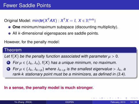
Fewer Saddle Points

Original Model: min{tr(XTAX) : XTX = I, X ∈ Rn×k }

One minimum/maximum subspace (discounting multiplicity).

All k -dimensional eigenspaces are saddle points.

However, for the penalty model:

TheoremLet f(X) be the penalty function associated with parameter µ > 0.

1 For µ ∈ (λk , λn), f(X) has a unique minimum, no maximum.2 For µ ∈ (λk , λk+p) where λk+p is the smallest eigenvalue > λk , a

rank-k stationary point must be a minimizers, as defined in (3.4).

In a sense, the penalty model is much stronger.


Error Bounds between Optimality Conditions

First order condition

Our penalty model: 0 = ∇f(X) , AX + µX(XTX − I);

Original model: 0 = R(X) , AY(X) − Y(X)(Y(X)TAY(X)),where Y(X) is an orthonormal basis of span{X}.

LemmaLet ∇f(X) (with µ > λk ) and R(X) be defined as above, then

‖R(X)‖F ≤ σ−1min(X)‖∇f(X)‖F , (3.5)

where σmin(X) is the smallest singular value of X. Moreover, for any globalminimizer X and any ε > 0, there exists δ > 0 such that whenever‖X − X‖F ≤ δ,

‖R(X)‖F ≤1 + ε√1 − λk/µ

‖∇f(X)‖F . (3.6)


Condition Number

Condition Number of the Hessian at Solution

κ(∇2f(X)) , λmax(∇2f(X))/λmin(∇2f(X))

Determining factor for asymptotic convergence rate of gradient methods

Lemma

Let X be a global minimizer of (3.2) with µ > λk . The condition number ofthe Hessian at X satisfies

κ(∇2f(X)

)≥

max (2(µ − λ1), (λn − λ1))

min (2(µ − λk ), (λk+1 − λk )). (3.7)

In particular, the above holds as an equality for k = 1.

Gradient methods may encounter slow convergence at the end.


Generalizations

Generalized eigenvalue problems: XTX = I → XTBX = I

Keep out undesired subspace: UTX = 0 (UT U = I)

Trace Minimization with Subspace Constraint

minX∈Rn×k

{tr(XTAX) : XTBX = I, UTX = 0}

Trace-Penalty Formulation

minX

12

tr(XTQTAQX) +µ

4‖XTQTBQX − I‖2F

where Q = I − UUT (QX = X − U(UT X)).

With changes of variables, all results still hold.


Algorithms for Trace-Penalty Minimization

Gradient Methods:

X ← X − α∇f(X). ∇f(X) = AX + µX(XTX − I)

First Order Condition:

∇f(X) = 0 ⇔ AX = X(I − XTX)µ

2 Types of Computations for ∇f(X):1 AX : O(k nnz(A))

2 X(XT X): O(k 2n) — BLAS3

(2) dominates (1) whenever k � nnz(A)/n

Gradient methods requires NO RR/Orth


Gradient Method

Preserve Full Rank

LemmaLet X j+1 be generated by

X j+1 = X j − αj∇f(X j)

from a full rank X j . Then X j+1 is rank deficient only if 1/αj is one of the kgeneralized eigenvalues of the problem:

[(X j)T∇f(X j)]u = λ[(X j)T (X j)]u.

On the other hand, if αj < σmin(X j)/||∇f(X j)||2, X j+1 is full rank.

Combined with previous results, there is a high probability of gettinga global minimizer by using gradient type methods.


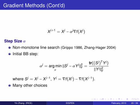
Gradient Methods (Cont’d)

X j+1 = X j − αj∇f(X j)

Step Size α

Non-monotone line search (Grippo 1986, Zhang-Hager 2004)

Initial BB step:

αj = arg minα||S j − αY j ||2F =

tr((S j)TY j)

||Y j ||2F

where S j = X j − X j−1, Y j = ∇f(X j) − ∇f(X j−1).

Many other choices


Current Algorithm

Framework:1 Pre-process — scaling, shifting, preconditioning2 Penalty parameter µ — dynamically adjusted3 Gradient iterations — main operations: X(XT X) and AX4 RR Restart — computing Ritz-pairs and restarting

(Further steps possible, but NOT used in comparison)5 Deflation — working on desired subspaces only6 Chebychev Filter — improving accuracy


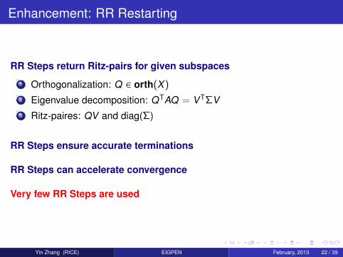
Enhancement: RR Restarting

RR Steps return Ritz-pairs for given subspaces

1 Orthogonalization: Q ∈ orth(X)

2 Eigenvalue decomposition: QTAQ = VTΣV3 Ritz-paires: QV and diag(Σ)

RR Steps ensure accurate terminations

RR Steps can accelerate convergence

Very few RR Steps are used


Section IV. Numerical Results and Conclusion


Pilot Tests in Matlab

Matrix: delsq(numgrid(’S’,102)); size: n = 10000; tol = 1e-3

CPU Time in Seconds

50 100 150 200 250 300 350 400 450 500

50

100

150

200

250

300

CP

U S

eco

nd

Number of Eigenvalues

eigs

lobpcg

eigpen

(a) with “-singleCompThread”

50 100 150 200 250 300 350 400 450 500

20

40

60

80

100

120

CP

U S

eco

nd

Number of Eigenvalues

eigs

lobpcg

eigpen

(b) without “-singleCompThread”


Experiment Environment

Running PlatformA single node of a Cray XE6 supercomputer (NERSC)

Two 12-core AMD ‘MagnyCours’ 2.1-GHz processors32 GB shared memory

System and language:Cray Linux Environment version 3Fortran + OpenMP

All 24 cores are used unless otherwise specified

Solvers Tested

ARPACK

LOBPCG

EIGPEN


Relative Error Measurements

Let x1 x2 · · · xk be computed Ritz vectors, and θi Ritz values.

Eigenvectors:

resi =‖Axi − θixi‖2

max(1, |θi |)

Eigenvalues:

eθ = maxi

|θi − λi |

max(1, |λi |),

Trace:

etrace =|∑k

i θi −∑k

i λi |

max(1, |∑k

i λi |)


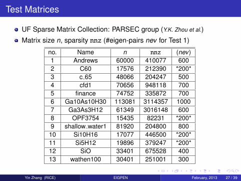
Test Matrices

UF Sparse Matrix Collection: PARSEC group (Y.K. Zhou et al.)

Matrix size n, sparsity nnz (#eigen-pairs nev for Test 1)

no. Name n nnz (nev)1 Andrews 60000 410077 6002 C60 17576 212390 *200*3 c 65 48066 204247 5004 cfd1 70656 948118 7005 finance 74752 335872 7006 Ga10As10H30 113081 3114357 10007 Ga3As3H12 61349 3016148 6008 OPF3754 15435 82231 *200*9 shallow water1 81920 204800 800

10 Si10H16 17077 446500 *200*11 Si5H12 19896 379247 *200*12 SiO 33401 675528 40013 wathen100 30401 251001 300


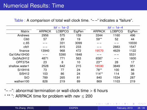
Numerical Results: Time

Table : A comparison of total wall clock time. “– –” indicates a “failure”.

tol = 1e−2 tol = 1e−4Matrix ARPACK LOBPCG EigPen ARPACK LOBPCG EigPen

Andrews 2956 575 159 3344 1160 496C60 57 29 19 59** 52 44c 65 – – 331 3099 – – – – 10030cfd1 – – 815 233 – – 2883 1547

finance 13940 968 472 19570 4629 1122Ga10As10H30 – – 5390 1848 – – – – 5531

Ga3As3H12 4871 771 563 6587 – – 1600OPF3754 23 8 10 23** 28 17

shallow water1 2528 642 215 18590 3849 951Si10H16 73 77 24 78** 100 86Si5H12 103 86 24 114** 114 38

SiO 789 265 81 840 1534 287wathen100 828 219 89 869 1103 219

“– –”: abnormal termination or wall-clock time > 6 hours“ ** ”: ARPACK time for problem with nev ≤ 200


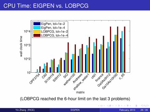
CPU Time: EIGPEN vs. LOBPCG

10

10^2

10^3

10^4

OPF37

54C60

Si10H

16

Si5H12 S

iO

wat

hen1

00

And

rews

shallow_w

ater

1cfd1

finan

ce

Ga3

As3

H12

Ga1

0As1

0H30

c_65

matrix

wa

ll clo

ck t

ime

EigPen, tol=1e−2

EigPen, tol=1e−4

LOBPCG, tol=1e−2

LOBPCG, tol=1e−4

(LOBPCG reached the 6-hour limit on the last 3 problems)


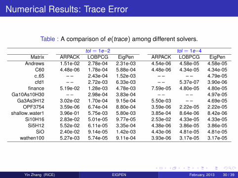
Numerical Results: Trace Error

Table : A comparison of e(trace) among different solvers.


Andrews 1.51e-02 2.78e-04 2.31e-03 4.54e-06 4.58e-05 4.58e-05C60 4.48e-06 1.78e-04 5.88e-04 4.48e-06 4.34e-05 4.34e-05c 65 – – 2.43e-04 1.52e-03 – – – – 4.79e-05cfd1 – – 2.72e-03 6.33e-03 – – 5.37e-07 3.90e-06

finance 5.19e-02 1.28e-03 4.78e-03 7.59e-05 4.80e-05 4.80e-05Ga10As10H30 – – 2.98e-04 3.83e-04 – – – – 4.97e-05

Ga3As3H12 3.02e-02 1.70e-04 9.15e-04 5.50e-03 – – 4.69e-05OPF3754 3.59e-06 6.74e-04 8.80e-04 3.59e-06 2.22e-05 2.22e-05

shallow water1 3.96e-01 5.75e-03 5.80e-03 3.85e-04 8.64e-06 8.42e-06Si10H16 2.83e-02 5.01e-05 9.77e-05 2.53e-02 4.33e-05 4.33e-05Si5H12 5.52e-02 6.11e-05 3.35e-04 4.38e-06 3.86e-05 3.86e-05

SiO 2.40e-02 9.14e-05 1.42e-03 4.43e-06 4.81e-05 4.81e-05wathen100 5.27e-03 5.74e-05 9.11e-04 3.93e-06 3.17e-05 3.17e-05


Numerical Results: Eigenvalue Error

Table : A comparison of maxi e(θi) among different solvers.


Andrews 1.01e-03 1.48e-05 1.06e-04 5.87e-09 1.07e-07 1.07e-07C60 1.72e-07 4.20e-06 7.48e-06 1.72e-07 9.01e-08 9.01e-08c 65 – – 5.73e-06 2.98e-05 – – – – 8.20e-07cfd1 – – 2.36e-01 5.37e-01 – – 1.43e-06 1.11e-05






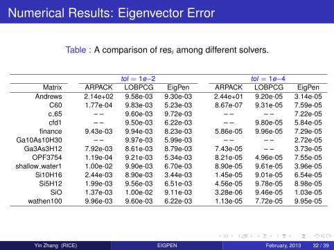
Numerical Results: Eigenvector Error

Table : A comparison of resi among different solvers.


Andrews 2.14e+02 9.58e-03 9.30e-03 2.44e+01 9.20e-05 3.14e-05C60 1.77e-04 9.83e-03 5.23e-03 8.67e-07 9.31e-05 7.59e-05c 65 – – 9.60e-03 9.72e-03 – – – – 7.22e-05cfd1 – – 9.50e-03 6.22e-03 – – 9.80e-05 5.84e-05






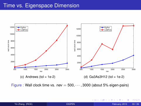
Time vs. Eigenspace Dimension

500 1000 1500 2000 2500 3000

2000

4000

6000

8000

10000

12000

nev

wa

ll clo

ck t

ime

EigPen

LOBPCG

(c) Andrews (tol = 1e-2)

500 1000 1500 2000 2500 3000

2000

4000

6000

8000

10000

12000

nev

wa

ll clo

ck t

ime

EigPen

LOBPCG

(d) Ga3As3H12 (tol = 1e-2)

Figure : Wall clock time vs. nev = 500, · · · , 3000 (about 5% eigen-pairs)


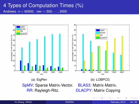
4 Types of Computation Times (%)Andrews. n = 60000. nev = 500, · · · , 3000

500 1000 1500 2000 2500 30000

10

20

30

40

50

60

70

80

90

nev

pe

rce

nta

ge

of

wa

ll c

lock t

ime

(%

)

SpMV

BLAS3

RR

DLACPY

(a) EigPen

500 1000 1500 2000 2500 30000

10

20

30

40

50

60

70

80

90

nevperc

enta

ge o

f w

all c

lock tim

e (

%)

SpMV

BLAS3

RR

DLACPY

(b) LOBPCG

SpMV: Sparse Matrix-Vector. BLAS3: Matrix-Matrix.RR: Rayleigh-Ritz. DLACPY: Matrix Copying


Parallel Speedup Factors

Recall: A single node of a Cray XE6 with 24 computing cores(two 12-core AMD “MagnyCours” 2.1-GHz processors)

Experiment setup:

Speedup-Factor for running on p cores:

Speedup-Factor(p) =run time using 1 corerun time using p cores

We run the 2 solvers for p = 2, 4, 8, 16, 24.


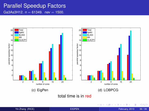
Parallel Speedup FactorsGa3As3H12. n = 61349. nev = 1500.

2 4 8 16 24

2

4

6

8

10

12

14

16

18

20

number of cores

pa

ralle

l sp

ee

du

p f

acto

r

Total

SpMV

BLAS3

RR

DLACPY

(c) EigPen

2 4 8 16 24

2

4

6

8

10

12

14

16

18

20

number of cores

pa

ralle

l sp

ee

du

p f

acto

r

Total

SpMV

BLAS3

RR

DLACPY

(d) LOBPCG

total time is in red


Preconditioning: Proof of Concept in Matlab

Preconditioned gradient method with pre-conditioner M ∈ Rn×n:

X j+1 = X j − αjM−1∇fµ(X j).

Matrix: c 65. n = 48066, nev = 500. M = LLT , L = ichol(A).

0 200 400 600 800 1000 120010

−3

10−2

10−1

100

101

102

103

104

105

||∇ f

µ(X

j )|| F

iteration

without preconditioning

(e) without preconditioning (Iter > 1200)

0 50 100 150 200 25010

−3

10−2

10−1

100

101

102

103

104

105

||∇ f

µ(X

j )|| F

iteration

with preconditioning

(f) with preconditioning (Iter < 300)

Figure : Gradient norm ‖∇fµ(X j)‖F Progress


Concluding Remarks

Why?

Eigenspace dimension tips balance of computation

Parallelism demands different thinking

How?

Trace-Penalty Model: penalty function is “exact”

Model yields fewer or even no saddle points

Orthogonalization and RR can be greatly reduced

What?

Efficient for moderate accuracy, numerically stable

Pre-conditioning can be effectively applied

BLAS3-rich, parallel scalability appears promising

Future: Enhancements/Refinements/Extensions


Thank you for your attention!


trace-penalty minimization for large-scale eigenspace...

Documents