Universitat Oberta de Catalunya (UOC)

Máster Universitario en Ciencia de Datos (Data Science)

TRABAJO FINAL DE MÁSTER

Área: Big Data / Machine Learning

Deep Learning for Image CaptioningAn Encoder-Decoder Architecture with Soft Attention

—————————————————————————–

Autor: Mario Gómez Martínez

Tutor: Anna Bosch Rué

Profesor: Jordi Casas Roma

—————————————————————————–

Valencia, June 28, 2019

Copyright

This work is licensed under Creative Commons Attribution-NonCommercial-ShareAlike 4.0

Spain License (CC BY-NC-SA 4.0 ES)

Esta obra está sujeta a una licencia de Reconocimiento-NoComercial-CompartirIgual 4.0

España de Creative Commons (CC BY-NC-SA 4.0 ES)

i

ii

FICHA DEL TRABAJO FINAL

Título del trabajo: Deep Learning for Image Captioning. An Encoder-Decoder Architecture with Soft Attention

Nombre del autor: Mario Gómez Martínez

Nombre del colaborador/a docente: Anna Bosch Rué

Nombre del PRA: Jordi Casas Roma

Fecha de entrega (mm/aaaa): 06/2019

Titulación o programa: Máster en Ciencia de Datos

Área del Trabajo Final: Aprendizaje automático

Idioma del trabajo: Inglés

Palabras clave Aprendizaje Profundo, Descripción de Imágenes

Código fuente https://github.com/magomar/image_captioning_with_attention

iii

iv

Dedicatoria

Dedicado a mi compañera, siempre ahí, para lo bueno y para lo malo, cercana, constante,

inspiradora...

... y a los tres retoños que inundan cada día de juegos inesperados y alegría arrolladora.

v

vi

Abstract

Automatic image captioning, the task of automatically producing a natural-language descrip-tion for an image, has the potential to assist those with visual impairments by explaining imagesusing text-to-speech systems. However, accurate image captioning is a challenging task that re-quires integrating and pushing further the latest improvements at the intersection of computervision and natural language processing fields

This work aims at building an advanced model based on neural networks and deep learningfor the automated generation of image captions.

Keywords: Deep Learning, Artificial Neural Networks, Automated image captioning

vii

viii

Resumen

El subtitulado automático de imágenes, la tarea de producir automáticamente una descripciónen lenguaje natural para una imagen, tiene el potencial de ayudar a las personas con discapaci-dades visuales a explicar las imágenes mediante sistemas de conversión de texto a voz. Sinembargo, el subtitulado preciso de imágenes es una tarea desafiante que requiere integrar yavanzar en la intersección de los campos de procesamiento de lenguaje natural y visión porcomputador.

Este trabajo pretende desarrollar un modelo basado en redes neuronales y aprendizaje pro-fundo para la generación automática de descripciones de imágenes.

Palabras clave: Aprendizaje Profundo, Redes Neuronales Artificiales, Descripción au-tomática de imágenes

ix

x

Contents

Abstract vii

Resumen ix

Index xi

List of Figures xv

List of Tables 1

1 Introduction 31.1 Motivation . . . . . . . . . . . . . . . . . . . . . . . . . . . . . . . . . . . . . . . 31.2 Goals . . . . . . . . . . . . . . . . . . . . . . . . . . . . . . . . . . . . . . . . . . 51.3 Methodology . . . . . . . . . . . . . . . . . . . . . . . . . . . . . . . . . . . . . 51.4 Planning . . . . . . . . . . . . . . . . . . . . . . . . . . . . . . . . . . . . . . . . 8

2 State of the Art 112.1 Task definition and classification of methods . . . . . . . . . . . . . . . . . . . . 122.2 Early work: methods that are not based on deep learning . . . . . . . . . . . . . 13

2.2.1 Retrieval-based . . . . . . . . . . . . . . . . . . . . . . . . . . . . . . . . 132.2.2 Template-based approaches . . . . . . . . . . . . . . . . . . . . . . . . . 16

2.3 Deep-learning approaches . . . . . . . . . . . . . . . . . . . . . . . . . . . . . . 172.3.1 Earlier Deep Models . . . . . . . . . . . . . . . . . . . . . . . . . . . . . 182.3.2 Multimodal learning . . . . . . . . . . . . . . . . . . . . . . . . . . . . . 192.3.3 The Encoder-Decoder framework . . . . . . . . . . . . . . . . . . . . . . 212.3.4 Attention-guided models . . . . . . . . . . . . . . . . . . . . . . . . . . . 232.3.5 Compositional architectures . . . . . . . . . . . . . . . . . . . . . . . . . 292.3.6 Other approaches . . . . . . . . . . . . . . . . . . . . . . . . . . . . . . . 31

2.4 Datasets and evaluation . . . . . . . . . . . . . . . . . . . . . . . . . . . . . . . 372.4.1 Datasets . . . . . . . . . . . . . . . . . . . . . . . . . . . . . . . . . . . . 37

xi

xii CONTENTS

2.4.2 Evaluation metrics . . . . . . . . . . . . . . . . . . . . . . . . . . . . . . 422.4.3 Summary of methods, datasets, metrics and benchmark results . . . . . . 45

3 Scope 553.1 Scope . . . . . . . . . . . . . . . . . . . . . . . . . . . . . . . . . . . . . . . . . 55

3.1.1 Research considerations . . . . . . . . . . . . . . . . . . . . . . . . . . . 563.1.2 Hardware requirements and time constraints . . . . . . . . . . . . . . . . 573.1.3 Software requirements . . . . . . . . . . . . . . . . . . . . . . . . . . . . 583.1.4 Summing up . . . . . . . . . . . . . . . . . . . . . . . . . . . . . . . . . . 58

3.2 The Encoder-Decoder architecture . . . . . . . . . . . . . . . . . . . . . . . . . . 593.2.1 From feature engineering to feature learning . . . . . . . . . . . . . . . . 593.2.2 The encoder-decoder architecture . . . . . . . . . . . . . . . . . . . . . . 593.2.3 Sequence to Sequence modelling . . . . . . . . . . . . . . . . . . . . . . . 613.2.4 Attention mechanisms . . . . . . . . . . . . . . . . . . . . . . . . . . . . 64

4 Model architecture and processes 734.1 Overview of the model architecture . . . . . . . . . . . . . . . . . . . . . . . . . 734.2 Encoder . . . . . . . . . . . . . . . . . . . . . . . . . . . . . . . . . . . . . . . . 754.3 Decoder . . . . . . . . . . . . . . . . . . . . . . . . . . . . . . . . . . . . . . . . 77

4.3.1 Attention . . . . . . . . . . . . . . . . . . . . . . . . . . . . . . . . . . . 784.4 Data pipelines . . . . . . . . . . . . . . . . . . . . . . . . . . . . . . . . . . . . . 80

4.4.1 Image pre-processing . . . . . . . . . . . . . . . . . . . . . . . . . . . . . 814.4.2 Text pre-processing . . . . . . . . . . . . . . . . . . . . . . . . . . . . . . 834.4.3 Dataset generation . . . . . . . . . . . . . . . . . . . . . . . . . . . . . . 85

4.5 Training the model . . . . . . . . . . . . . . . . . . . . . . . . . . . . . . . . . . 854.5.1 Loss function . . . . . . . . . . . . . . . . . . . . . . . . . . . . . . . . . 864.5.2 Teacher forcing . . . . . . . . . . . . . . . . . . . . . . . . . . . . . . . . 87

4.6 Inference and validation . . . . . . . . . . . . . . . . . . . . . . . . . . . . . . . 884.6.1 Greedy Search . . . . . . . . . . . . . . . . . . . . . . . . . . . . . . . . . 894.6.2 Exhaustive Search . . . . . . . . . . . . . . . . . . . . . . . . . . . . . . 904.6.3 Beam search . . . . . . . . . . . . . . . . . . . . . . . . . . . . . . . . . . 90

4.7 Implementation . . . . . . . . . . . . . . . . . . . . . . . . . . . . . . . . . . . . 92

5 Experiments 935.1 Dataset . . . . . . . . . . . . . . . . . . . . . . . . . . . . . . . . . . . . . . . . 935.2 Experiments . . . . . . . . . . . . . . . . . . . . . . . . . . . . . . . . . . . . . . 95

5.2.1 Experimental setup . . . . . . . . . . . . . . . . . . . . . . . . . . . . . . 95

CONTENTS xiii

5.2.2 Overview of the experiments . . . . . . . . . . . . . . . . . . . . . . . . . 965.2.3 Demonstrative examples . . . . . . . . . . . . . . . . . . . . . . . . . . . 100

6 Conclusions 1076.1 What I learned . . . . . . . . . . . . . . . . . . . . . . . . . . . . . . . . . . . . 107

6.1.1 What I would have changed . . . . . . . . . . . . . . . . . . . . . . . . . 1086.1.2 What I did not expect . . . . . . . . . . . . . . . . . . . . . . . . . . . . 109

6.2 Future work . . . . . . . . . . . . . . . . . . . . . . . . . . . . . . . . . . . . . . 1096.3 Concluding remarks . . . . . . . . . . . . . . . . . . . . . . . . . . . . . . . . . . 110

Bibliography 111

xiv CONTENTS

List of Figures

1.1 Image captioning can help millions with visual impairments by converting imagescaptions to text. Image by Francis Vallance (Heritage Warrior), used under CCBY 2.0 license. . . . . . . . . . . . . . . . . . . . . . . . . . . . . . . . . . . . . 4

1.2 Illustration of images and captions in the Conceptual Captions dataset.Clockwisefrom top left, images by Jonny Hunter, SigNote Cloud, Tony Hisgett, Resolute-SupportMedia. All images used under CC BY 2.0 license. . . . . . . . . . . . . . 6

1.3 Process diagram showing the relationship between the different phases of CRISP-DM. Image by Kenneth Jensen, used under CC BY-SA 3.0 license.. . . . . . . . 7

2.1 Structure of multimodal neural learning models for image captioning . . . . . . 20

2.2 Structure of image captioning methods based on the encoder-decoder framework 21

2.3 Structure of image captioning methods based on the encoder-decoder framework 24

2.4 Structure of image captioning methods based on the encoder-decoder framework 29

2.5 Examples of images and their descriptions across various benchmark datasets . . 41

3.1 The encoder-decoder architecture. . . . . . . . . . . . . . . . . . . . . . . . . . . 59

3.2 Convolutional encoder-decoder for image segmentation in the SeqNet architec-ture (Badrinarayanan et al., 2017) . . . . . . . . . . . . . . . . . . . . . . . . . . 60

3.3 Recurrent encoder-decoder for automated email answering. The model is giveninput a sentence and produces a response in the same language. Source: GoogleAI Blog . . . . . . . . . . . . . . . . . . . . . . . . . . . . . . . . . . . . . . . . 61

3.4 Encoder-decoder combining CNN and LSTM for image captioning. Source: Yun-jey Choi’s implementation of the Show and Tell model (Vinyals et al., 2015). . . 62

3.5 The sequence to sequence model architecture. . . . . . . . . . . . . . . . . . . . 63

3.6 Layers in seq2seq model. . . . . . . . . . . . . . . . . . . . . . . . . . . . . . . . 63

3.7 Sequence to sequence model predicting with greedy search. . . . . . . . . . . . . 64

3.8 The encoder-decoder model with additive attention mechanism in (Bahdanauet al., 2015) . . . . . . . . . . . . . . . . . . . . . . . . . . . . . . . . . . . . . . 66

xv

xvi LIST OF FIGURES

3.9 Alignment matrix of an French sentence and its English translation. Source: Fig3 in (Bahdanau et al., 2015)) . . . . . . . . . . . . . . . . . . . . . . . . . . . . 67

3.10 The current word is in red and the size of the blue shade indicates the activationlevel. Source: (Cheng et al., 2016). . . . . . . . . . . . . . . . . . . . . . . . . . 69

3.11 Caption generation example:A woman is throwing a frisbee in a park. Source:(Xu et al., 2015). . . . . . . . . . . . . . . . . . . . . . . . . . . . . . . . . . . . 69

3.12 Comparative of soft (top) vs hard (bottom) attention during caption generation.Source: (Xu et al., 2015). . . . . . . . . . . . . . . . . . . . . . . . . . . . . . . . 70

3.13 Comparative of global (left) vs local (right) attention in the seq2seq model.Source: (Luong et al., 2015). . . . . . . . . . . . . . . . . . . . . . . . . . . . . . 71

4.1 Overview of the model architecture: encoder, decoder and attention mechanism 744.2 Detailed architecture showing the layers of each component . . . . . . . . . . . . 754.3 Overview of the Inception v3 network architecture. Source Google’s Advanced

Guide to Inception v3 on Cloud TPU . . . . . . . . . . . . . . . . . . . . . . . . 764.4 Detailed architecture of the additive soft attention mechanism . . . . . . . . . . 804.5 Overview of the data preparation pipeline . . . . . . . . . . . . . . . . . . . . . 814.6 Teacher forcing for image captioning training. The expected word is used as

input of the network at each timestep . . . . . . . . . . . . . . . . . . . . . . . . 884.7 Word-by-word caption generation . . . . . . . . . . . . . . . . . . . . . . . . . . 884.8 The four numbers under each time step represent the conditional probabilities of

generating "A", "B", "C", and "<end>" at that time step. At each time step,greedy search selects the word with the highest conditional probability. . . . . . 89

4.9 The four numbers under each time step represent the conditional probabilitiesof generating "A", "B", "C", and "<end>" at that time step. At time step 2,the word "C", which has the second highest conditional probability, is selected. . 90

4.10 The beam search process. The beam size is 2 and the maximum length of theoutput sequence is 3. The candidate output sequences are A, C, AB, CE, ABD,and CED. . . . . . . . . . . . . . . . . . . . . . . . . . . . . . . . . . . . . . . 91

5.1 Image caption examples. Source: COCO Image Captioning Task . . . . . . . . . 935.5 Correlation matrix for the numeric hyperparameters and the performance metrics 995.6 Evolution of loss and performance as training progresses . . . . . . . . . . . . . 1005.7 Ground Truth: A man standing on a tennis court holding a tennis racquet. . . . 1025.8 Predicted: a tennis player is getting ready to hit a tennis ball. . . . . . . . . . . 1025.9 Ground Truth: Two males and a female walking in the snow carrying a ski sled

and snowboard. . . . . . . . . . . . . . . . . . . . . . . . . . . . . . . . . . . . . 103

LIST OF FIGURES xvii

5.10 Predicted: a person riding skis ride down a snowy hills. . . . . . . . . . . . . . . 1035.11 Ground Truth: A man sitting on the back of a red truck. . . . . . . . . . . . . . 1045.12 Predicted: a group of people are posing for a red covered lawn. . . . . . . . . . . 1045.13 Ground Truth:a man is holding a piece of food with chocolate in it. . . . . . . . 1055.14 Predicted: A person holding a piece of chocolate cake with a chocolate cake. . . 105

xviii LIST OF FIGURES

List of Tables

1.1 Main tasks and milestones. . . . . . . . . . . . . . . . . . . . . . . . . . . . . . . 8

2.1 Summary of published research on the automatic image description problem. . . 142.2 Classification of retrieval-based image captioning. . . . . . . . . . . . . . . . . . 162.3 Summary of benchmark datasets. . . . . . . . . . . . . . . . . . . . . . . . . . . 382.4 Classification of deep-learning methods . . . . . . . . . . . . . . . . . . . . . . . 472.4 Classification of deep-learning methods . . . . . . . . . . . . . . . . . . . . . . . 482.5 Summary of non neural methods, datasets and evaluation metrics. . . . . . . . . 492.6 Summary of neural methods, datasets and metrics . . . . . . . . . . . . . . . . . 492.6 Summary of neural methods, datasets and metrics . . . . . . . . . . . . . . . . . 502.6 Summary of neural methods, datasets and metrics . . . . . . . . . . . . . . . . . 512.7 Comparison of methods on the Flickr30K dataset . . . . . . . . . . . . . . . . . 522.8 Comparison of methods on the MSCOCO dataset . . . . . . . . . . . . . . . . . 53

3.1 summary table of several popular attention mechanisms and corresponding align-ment score functions . . . . . . . . . . . . . . . . . . . . . . . . . . . . . . . . . 68

4.1 Summary of popular ConvNets pretrained on the ImageNet dataset . . . . . . . 82

5.1 Evaluation results. Model trained for 30 epochs. No regularization applied. . . . 975.2 Some results of training and validation without normalization . . . . . . . . . . 1005.3 Some results of training and validation with dropout = 0.3 . . . . . . . . . . . . 101

2 LIST OF TABLES

Chapter 1

Introduction

1.1 Motivation

The web provides a vast amount of information, including a lot of text, but it is increasinglydominated by visual information, both static (pictures) and dynamic (videos). However, muchof that visual information is not accessible to those with visual impairments, or with slow in-ternet speeds that prohibit the loading of images. Image captions, manually added by contentproviders (typically by using the Alt-text HTML tag), is one way to make this content moreaccessible, so that a text-to-speech system can be applied to generate a natural-language de-scription of images and videos. However, existing human-curated image descriptions are addedfor only a very small fraction of web images. Thus, there is great interest in developing methodsto automatically generate image descriptions.

Automatic image description, also known in the research community as image captioning,can be defined as the task of automatically generating a description of an image using naturallanguage. It is a very challenging problem that encompasses two kinds of problems: the problemof understanding an image, which is a Computer Vision (CV) task and the problem ofgenerating a meaningful and grammatically-correct description of the image, which is a kind ofNatural-Language Processing (NLP) task. Therefore, to tackle this task it is necessaryto advance the research in the two fields, CV and NLP, as well as promoting the cooperationof both communities to address the specific problems arising when combining both tasks.

Figure 1.1 shows an example of the automatic image generation tasks addressed by thisproject.

There are other use cases in which automatically generated image captions may help. Gen-erally speaking, any domain in which images need to be interpreted by humans, but humanavailability is scarce, or the task at hand is tedious, may surely benefit from algorithms able toautomatically generate textual image descriptions.

3

4 Introduction

Figure 1.1: Image captioning can help millions with visual impair-ments by converting images captions to text. Image by Francis Val-lance (Heritage Warrior), used under CC BY 2.0 license.

A vast area of application is that of Concept-Based Image Retrieval. This kind of task,also named as "description-based" or "text-based" image indexing/retrieval, refers to retrievalfrom text-based indexing of images that may employ keywords, subject headings, captions, ornatural language text. The main problem with this approach to image retrieval is the scarcityof image descriptions, since having humans manually annotate images by entering keywordsor descriptions in a large database can be very tedious and time consuming 1. Therefore,automatic image description may be of great utility, and it can be applied to many areasrequiring image indexing and retrieval, such as biomedicine, education, digital libraries, etc., aswell as general web search. In addition, there is an extra benefit in using captions vs keywords:image captions are semantically richer and more sophisticated, thus allowing for more complexqueries to improve the precision of the search.

Another area where automatic image captioning may be of great utility is the analysisand extraction of information from videos. Some video monitoring tasks are very boring andtedious. An automated mechanism to describe scenes in video footage will be of great utilityfor creating summaries or monitoring specific situations and events. 2.

Image captioning can also be used to improve image indexing since it provides a more so-phisticated and semantically rich description that image classification or simple image tagging.This kind of semantic indexes would be very very useful for any kind of Content-Based ImageRetrieval application, which would help improve any king of Content-Based Image Retrieval.This kind of Having images automatically generated captions for images that originally hasn’tbeen described, would help to find images based on a complex description rather than a simple

1This is one of the reasons explaining the upswing of Content-Based Image Retrieval, which uses content de-rived from the visual properties of the image, like color, textures, and shape, instead of semantic and descriptivedata such as keywords and captions

2As an interesting example, Shell is conducting a pilot study using deep-learning to automatically monitorvideo footage in order to identify safety hazards and generate alerts (link)

1.2. Goals 5

collection of tags.

1.2 Goals

This project aims at advancing in the task of automatically generating image descriptions.That is the ultimate goal of the project. However, in order to achieve such an abstract goal,we decompose it into various subgoals, as follows:

1. Get a solid understanding of the problem at hand and review the state-of-art solutionsto it

2. Get practical knowledge on the technologies required to solve this problem

3. Develop a model using a benchmark dataset like the Flickr30K

4. Scale the model to a larger benchmark dataset such as the COCOLin et al. (2014) datasetor the more recent Conceptual Captions Dataset by Google Sharma et al. (2018) (seeFig. 1.2).

5. Evaluate the model, ideally partaking in some challenge or competition, like the onesusing the COCO dataset or the Conceptual Captions dataset.

1.3 Methodology

This project is mainly an academical, research-oriented project, so it follows a process modelwhich is common for this kind of projects. For instance, it includes an extensive survey ofthe state of the art and proposes a model to solve the target problem. However, this projectwill also include the development of a software artifact to implement the proposed model usingreal data. As such, this project can benefit from a data-analytic model as the well known andwidely adopted CRISP-DM. CRISP-DM, which stands for Cross-Industry Standard Processfor Data Mining, is an open standard process model and an industry-proven methodology toguide data mining projects.

As a methodology, it includes descriptions of the typical phases of a project, the tasksinvolved with each phase, and an explanation of the relationships between these tasks.

As a process model, CRISP-DM provides an overview of the data mining life cycle.Figure 1.3 depicts the relationships between the different phases of the CRISP-DM model.

The sequence of the phases is not strict and moving back and forth between different phases isoften required. The arrows in the process diagram indicate the most important and frequent

6 Introduction

Figure 1.2: Illustration of images and captions in the ConceptualCaptions dataset.Clockwise from top left, images by Jonny Hunter,SigNote Cloud, Tony Hisgett, ResoluteSupportMedia. All imagesused under CC BY 2.0 license.

1.3. Methodology 7

dependencies between phases. The outer circle in the diagram symbolizes the cyclic nature ofdata mining itself. A data mining process continues after a solution has been deployed. Thelessons learned during the process can trigger new, often more focused business questions andsubsequent data mining processes will benefit from the experiences of previous ones.

Figure 1.3: Process diagram showing the relationship between thedifferent phases of CRISP-DM. Image by Kenneth Jensen, used underCC BY-SA 3.0 license..

The process model consists of six major phases:

• Business Understanding: Includes in-depth analysis of the business objectives andneeds. The situation is assessed and the goals of the project are defined. This shouldfollow the setting up of a plan to proceed.

• Data Understanding: Conduct initial or exploratory data analysis to become familiarwith data and identify potential problems. Examine the properties of data and verify itsquality by answering questions concerning the completeness and accuracy of the data.

• Data Preparation: After the data sources are completely identified, proper selection,cleansing, constructing and formatting should be done before modeling.

• Modeling: Modeling is usually conducted in multiple iterations, which involves runningseveral models using the default parameters and then fine-tune the parameters or revertto the data preparation phase for additional preparation. Usually, there are different waysto look at a given problem, so it is convenient to build multiple models,

8 Introduction

• Evaluation: The results of models are evaluated in the backdrop of business intentions.New objectives may sprout up owing to the new patterns discovered. This is, in fact, aniterative process, and the decision whether to consider them or not has to be made in thisstep before moving on to the final phase

• Publication. The final information gathered has to be presented in a usable manner tothe stakeholders. This has to be done as per their expectations and business requirements.

1.4 Planning

This section briefly describes the initial planning established to accomplish this Final Master’sThesis.

1.4.0.1 Original planning

Table 1.1: Main tasks and milestones.

Phase End Description

1 3/3/2019 Definition and planning2 24/3/2019 State of the Art3 19/5/2019 Development4 9/6/2019 Complete this report5 16/6/2019 Presentation

Table 1.1 sums up the original planning for this project. It consisted of 5 phases:

Phase 2 is devoted to surveying the state of the art. This phase will encompass the followingtasks:

• Reviewing relevant bibliography

• Studying the problem domain (business understanding), and becoming familiar with thedata. At this stage, we would also start preparing the data for the modeling stage

Phase 3 is intended to design and develop a software artifact. It is the longest phase, andincludes the following tasks:

• Preparing the data. Although data preparation could be started during phase 2, de-pending on the chosen models it could be necessary to conduct some additional datapreparation operations

1.4. Planning 9

• Generating one or various models. We plan at creating at least two models, one thatwould replicate existing work, and another one to explore new ideas and try to beat thebaseline model.

• Evaluating the models, and very specifically, compare our model against the replicatedmodel.

• Publication: We consider two courses of action: a) participating in the Microsoft COCOImage Captioning Challenge, and b) delivering some product to the final user, althoughit would be a very basic prototype given the time available.

Phase 4 is conceived for completing this report. This phase would probably overlap withsome of the tasks in phase 3 that will require additional time, like the evaluation of the modelsand the participation in challenges.

Phase 5 is the last one. At this phase, the results of the project should be published, includingboth the report and any code and documentation. Finally, the project has to exposed anddefended publicly, to be evaluated by an academic board.

10 Introduction

Chapter 2

State of the Art

Recently there has been an upsurge of interest in problems that require a combination oflinguistic and visual information. Besides, the rise of social media in the web has made availablea vast amount of multimodal information, like tagged photographs, illustrations in newspaperarticles, videos with subtitles, and multimodal feeds on social media. To tackle combinedlanguage and vision tasks and to exploit the large amounts of multimodal information, the CVand NLP communities have been increasingly cooperating, for example by organizing combinedworkshops and conferences. One such area of research in the intersection of both worlds isautomatic image description.

Automatic image description can be defined as the task of automatically generating adescription of an image using natural language. It is a very challenging problem that combinestwo different problems into a single task: on the one hand, there is the problem of understandingan image, which belongs to theComputer Vision (CV) field, one the other hand, there is alsothe problem of generating a meaningful and grammatically-correct description of the image,which belongs to the Natural-Language Processing (NLP) field, and to be more precise,it belongs to the class of Natural-Language Generation (NLG) problems.

Both CV and NLP are challenging fields themselves. While both fields share commontechniques rooted in artificial intelligence and machine learning, they have historically developedseparately, with little interaction between their scientific communities. Recent years have seenconsiderable advances in both fields, to a great extent thanks to the application of deep-learningtechniques and the recent advances in this area. This chapter presents a brief survey of therecent literature on this topic, including some antecedents, but focusing primarily on the recentadvances coming from the application of Deep Learning technology since this is our maininterest.

The chapter is organized in various sections. The first section is devoted to further delimitingthe task at hand as well as introducing a classification schema for the different approaches to the

11

12 State of the Art

problem. Subsequent sections review relevant publications organized according to the providedclassification scheme. Finally, there is a section describing the datasets used by the communityto benchmark their models and a short discussion on the evaluation metrics for this kind oftasks.

2.1 Task definition and classification of methods

We have already defined the task of automatic image description as the task of automaticallygenerating a description of an image using natural language generation. However, this defini-tion is too generic to precisely characterize the task we are interested in. For example, whenpresented with certain image, an algorithm may generate a list of labels describing different el-ements of the image, or it may describe technical features of the image, such as the dimensions,the predominant colors, brightness, etc. Therefore, we need a more concrete definition of thetask.

When talking about automatic image description, we refer to descriptions that meetthree properties:

• Descriptions that are relevant, that is descriptions that talk about the elements of theimage.

• Descriptions that are expressed as natural language, using grammatically correct sen-tences

• Descriptions that are comprehensive but concise at the same time, that is, the descriptionshould aim at summing up the important elements of the image, not just describing it.

From the CV point of view, this task requires full image understanding: the descriptionshould demonstrate or pretend a good understanding of the scene, far beyond simply recognizingthe objects in the image. This means that the description is able to capture relations betweenthe objects in the scene, and the actions happening there.

From the NLP point of view, this task requires sophisticated natural language gener-ation (NLG), which involves: selecting which aspects to talk about (content selection), sortingand organizing the content to be verbalized (text planning), and finally generating a semanti-cally and syntactically correct sentence (Surface realization).

Intuitively, descriptions should be easy to understand by a person, and that person shouldbe able to grasp the essence of the image, to create a mental model of the image without actuallyseeing it. The description task can become even more challenging when we take into accountuser-specific tailored descriptions. For instance, when describing the paintings available in amuseum, a tourist may require a different description than a librarian or an art critic.

2.2. Early work: methods that are not based on deep learning 13

Since 2011 there has been a considerable advance in challenging CV tasks, to a great extentfostered by the application of deep learning models and the availability of large corpus of dataavailable to researchers. More recently, a similar process seems to be occurring in the NLPfield. Not surprisingly, these advances in both CV and NLP have also propelled a new wave ofinterest in cross-disciplinary research problems involving both areas of research, and automaticimage description is a very good example. As a consequence, the CV and NLP communitieshave increased cooperation, for example by organizing joint workshops over the past few years.These efforts have resulted in a surge of new models, datasets and evaluation measures, whichis reflected in the increase of publications, especially from 2014.

In order of ease of review, understanding, and comparison of the growing amount of researchon the topic, existing surveys have proposed various schemes to classify the models being used.

One the one hand, the survey by Bernardi et al. (2017) proposes a classification systembased on two dimensions and only three categories. On the other hand, Bai and An (2018)organize the existing research according to the kind of architecture or framework used, resultingin a more fine-grained classification with 8 categories.

After comparing both approaches to classify the existing research, we prefer the approachadopted by Bai and An (2018) as we consider it more precise and descriptive, resulting in afiner granularity; while the classification by Bernardi et al. (2017) is more abstract, resulting ina coarser granularity. A more recent survey by Hossain et al. (2019) takes the same approachfound in (Bai and An, 2018) with a more focused review of deep-learning based models andreferences to the most recent work published so far.

Below we provide a short overview of the publications covered in this survey organized intocategories and sorted by publication year:

2.2 Early work: methods that are not based on deep learn-

ing

This section reviews the initial attempts to solve the image captioning problem. All thesemethods have in common that they do not use deep learning techniques. We divide them intotwo groups: retrieval based approaches and template-based approaches.

2.2.1 Retrieval-based

Early work on the topic was often based on the use of retrieval-based approaches, also referredto as transfer-based approaches. These approaches usually follow a two steps process. Duringthe first step, given a query image, a candidate set of similar images is retrieved using content-

14 State of the Art

Table 2.1: Summary of published research on the automatic imagedescription problem.

Approach Representative research

Retrieval-based Farhadi et al. (2010); Ordonez et al. (2011); Gupta et al. (2012);Kuznetsova et al. (2012); Hodosh et al. (2013); Kuznetsova et al.(2014); Mason and Charniak (2014); Hodosh and Hockenmaier(2013)

Template-based Yang et al. (2011); Kulkarni et al. (2011); Li et al. (2011); Mitchellet al. (2012); Ushiku et al. (2015)

Earlier Deep Models Socher et al. (2014); Karpathy et al. (2014); Ma et al. (2015); Yanand Mikolajczyk (2015); Lebret et al. (2015a); Yagcioglu et al.(2015)

Multimodal learning Kiros et al. (2014a); Mao and Yuille (2015); Karpathy and Fei-Fei(2015); Chen and Zitnick (2015)

Encode-Decoder framework Kiros et al. (2014b); Vinyals et al. (2015); Donahue et al. (2015);Jia et al. (2015); Wu et al. (2016); Pu et al. (2016b); Gan et al.(2017a); Hao et al. (2018)

Compositional architectures Fang et al. (2015); Tran et al. (2016); Ma and Han (2016); Orugantiet al. (2016); Wang et al. (2016); Fu et al. (2017); Gan et al. (2017b)

Attention-guided Xu et al. (2015); You et al. (2016); Yang et al. (2016); Zhou et al.(2017); Khademi and Schulte (2018); Anderson et al. (2018b);Jiang et al. (2018)

Describing novel objects Mao et al. (2015); Hendricks et al. (2016)Other deep learning meth-ods

Pu et al. (2016a); Dai et al. (2017); Shetty et al. (2017); Ren et al.(2017); Rennie et al. (2017); Zhang et al. (2017); Anderson et al.(2018a); Feng et al. (2018); Gu et al. (2018); Li et al. (2018); Liand Chen (2018); Lindh et al. (2018)

based image retrieval techniques, which are based on global image features extracted from theimage. During the second step, a re-ranking of the retrieved images is computed using a varietyof methods. Finally, the caption of the top image is returned, or a new caption is composed ofthe captions of the top-n ranked images.

Farhadi et al. (2010) use a meaning space consisting of <object, action, scene> triplets tolink images and sentences. Their model takes an input image, map it into the meaning spaceby solving a Markov Random Field, and use Lin’s information-based similarity measure (Lin,1998) to determine the semantic distance between the query image and the pool of availablecaptions. Finally, the semantically closest sentence is used as the image description.

The IM2TEXT model by Ordonez et al. (2011) uses the scene-centered descriptors of theGIST model (Oliva and Torralba, 2006; Torralba et al., 2008) to retrieve a set of similar imagesas a baseline, then these images are ranked using a classifier trained over a range of object

2.2. Early work: methods that are not based on deep learning 15

detectors and scene classifiers specific to the entities mentioned in the candidate descriptions.Finally, the caption of the top-ranked image is returned.

Kuznetsova et al. (2012) take on the work by Ordonez et al. (2011) with some notabletwists: instead of retrieving a candidate set of images using content –visual– features, theirmodel start by running the detectors and scene classifiers used in the re-ranking step of theIM2TEXT model to extract and represent the semantic content of the query image. Then,instead of performing a single retrieval step to get neighbors of the query image, their modelcarries out a separate retrieval step for each visual entity detected in the query image. The resultof this step is a collection of phrases of different type (noun and verb phrases and prepositionalphrases). Finally, a new sentence is composed from a selected set of phrases using a constraintoptimization approach. A refinement of the former approach is presented in Kuznetsova et al.(2014), based on the use of tree structures to improve the sentence generation process.

Gupta et al. (2012) combine the image features of the GIST model with RGB and HSV colorhistograms, Gabor and Haar descriptors, and SIFT (Lowe, 2004) descriptors for the retrievalstep. Then, instead of using the visual features for the ranking step, their model relies on thetextual descriptions of the retrieved images, which are segmented to obtain phrases of a differenttype. This model takes the phrases associated to the retrieved images, rank them based onimage similarity, and integrate them to get triples of the form ( ((attribute1, object1), verb),(verb, prep, (attribute2, object2)), (object1, prep, object2) ). Finally, the tree top-n triplets areused to generate an image description.

Hodosh and Hockenmaier (2013) employ a Kernel Canonical Correlation Analysis (KCCA)(Bach and Jordan, 2003) technique to project images and text items into a common space,where training images and their corresponding captions are maximally correlated. In the newcommon space, cosine similarities between images and sentences are calculated to rank thesentences, which are then used to select the top-n captions. This work is highly focused on theproblems associated with existing benchmarks datasets and the evaluation metrics, and as aresult, the authors introduce a new dataset composed of 8000 images annotated with 5 captionsper image and propose a new metric based on binary judgments of image descriptions.

Mason and Charniak (2014) use visual similarity to retrieve a set of candidate captionedimages. Second, a word probability density conditioned on the query image is computed fromthe retrieved captions. Finally, the candidate captions are scored using the word probabilitydensity and the one with the highest score is selected.

A detailed analysis of the literature reviewed here reveals at least two dimensions that mayfurther help in understanding and organizing the research: on the one hand, some approachessimply select one of the retrieved sentences as the image caption, while others compose a newcaption by combining elements from several sentences; on the other hand, some approaches use

16 State of the Art

visual detectors to find similar images (Content-Based Image Retrieval), while other approachesuse conceptual information (Concept-Based Image Retrieval), or use a combination of visualand conceptual information for the retrieval step. Table 2.2 sums up the various dimensionsused to classify retrieval-based methods to the image captioning problem.

Table 2.2: Classification of retrieval-based image captioning.

Approach Representative research

Information modality Select one caption Compose captionVisual Farhadi et al. (2010); Mason and

Charniak (2014)Gupta et al. (2012)

Conceptual Ordonez et al. (2011) Kuznetsova et al. (2012, 2014)Hybrid Hodosh and Hockenmaier (2013)

The main disadvantage of Retrieval-Based approaches comes from the reuse of existingimages. The sentences used to describe images in the past may be completely inadequatefor describing a new image. Although some of the proposed models are able to composenew sentences rather than just returning one of the stored sentences, these are still based onpreviously used sentences, so the result may still be unsuited for describing the query image.This limitation was strikingly evident with the use of small datasets, therefore, perhaps theproblem would be alleviated with the use of very large datasets as the ones that have appearedrecently Lin et al. (2014); Sharma et al. (2018).

2.2.2 Template-based approaches

Another group of early attempts to solve the automatic image captioning problem takes somekind of template-based approach. Unlike retrieval based approaches, template-based approachesanalyze the query image to generate concepts and then use some kind of constraining mechanismto compose a sentence. The constraints typically adopt the form of a template, but can alsobe specified as grammar rules.

For example, Yang et al. (2011) use a quadruplet consisting of<Noun-Verb-Scene-Preposition>as template for generating image descriptions. The process starts with the execution of detec-tion algorithms to estimate objects and scenes in the image, and then apply a language modeltrained over the Gigaword corpus1 to compute nouns, verbs, scenes and prepositions that mightappear in the caption. Finally, they apply Hidden Markov Model Inference to compute prob-abilities for all the elements and use the elements with the highest probabilities to fill thetemplate and generate a new sentence.

1https://catalog.ldc.upenn.edu/LDC2003T05

2.3. Deep-learning approaches 17

Kulkarni et al. (2011) employ Conditional Random Field (CRF) to determine image con-tents, which results in a graph with nodes corresponding to objects in the image, object at-tributes, and spatial relationships between objects. Unary potential functions are computedfor nodes in the graph, while pairwise potential functions are obtained on a collection of ex-isting descriptions. Afterward, CRF inference is used to determine the image contents to bedescribed, and finally, a sentence template is applied to generate a sentence using the selectedcontent.

Li et al. (2011) use visual models to detect objects, attributes and spatial relationships,and. Then, they resort to web-scale n-gram data to compute frequency counts of possible n-gram sequences to fill a triplet defined as <(adj1, obj1), prep, (adj2, obj2)>. Finally, dynamicprogramming is applied to find an optimal set of phrases that constitute the description of thequery image.

Mitchell et al. (2012) apply algorithms that are able to represent an image as an <objects,actions, spatial relationships> triplet. Syntactically informed word co-occurrence statistics arecomputed and used by a sentence generator to filter and constrain the output of the imageprocessor using tree structures.

The aforementioned works in this section produce new sentences based on individual words(nouns, adjectives, verbs, prepositions, etc.) that generated in a piece-wise manner from thequery image, and these words are later connected according to certain grammar model. Toimprove on this approach, some authors have proposed the use of phrases instead of individualwords. In particular, Ushiku et al. (2015) present a method named Common Subspace for Modeland Similarity (CoSMoS). CoSMoS obtains a subspace in which all feature vectors associatedwith the same phrase are mapped as mutually close, classifiers for each phrase are learned,and training samples are shared among co-occurring phrases. Phrases estimated from a queryimage are connected by using multi-stack Beam search to generate a description.

Template-based approaches to automatic image captioning may improve the relevance ofthe resulting captions when compared with retrieval based approaches, template-based captionstend to be too rigid, thus resulting in a lack of naturality when compared to human-writtensentences.

2.3 Deep-learning approaches

Convolutional Neural Networks (CNN) were first introduced by Yann LeCun in 1998 (Lecunet al., 1998), but it was not until more than a decade later than they started to shine. In 2012,a large, deep CNN (Krizhevsky et al., 2012) was used to win, by an incredibly wide margin, the2012 ImageNet Large-Scale Visual Recognition Challenge. From that turning point, the field

18 State of the Art

has attracted the attention of researchers from various fields and gained howling popularity.The success of CNN and other deep learning models was due to a great extent to its impressiveresults in many challenging problems, prominently in the fields of Computer Vision and NaturalLanguage Processing, where deep-learning models have become the current state-of-the-art.Not surprisingly, researchers have attempted to apply deep neural networks to solve problemsin the interstice of both fields, CV and NLP, includes the problem of automatically generatingimage descriptions.

Recent advances in the field have been achieved with the introduction of new architec-tures and frameworks, accompanied by increasingly larger datasets to feed those deep neuralnetworks. Therefore, there is a wide repertoire of methods for tackling the image captioningtasks. This section presents the contributions to the field organized according to the kind ofarchitecture or framework utilized, with one subsection per category

2.3.1 Earlier Deep Models

Encourage by the success of CNN to solve image classification tasks, researchers began incor-porating deep models into their image captioning methods, yet still influenced by the retrieval-based and template-based methods. Image captioning was formulated as a multi-modalityembedding Frome et al. (2013) and ranking problem.

Socher et al. (2014) use dependency-tree recursive neural networks (DT-RNN) to representphrases and sentences as compositional vectors. Another deep neural network (Le et al., 2011)is used to extract visual features from the images. Both types of features are mapped into acommon space by using a max-margin objective function. After training, sentence retrieval isperformed based on similarities between representations of images and sentences in the commonspace.

Karpathy et al. (2014) introduce a twist in the previous model by working at a finer level,that is, instead of modeling full images, they work on a finer level by embedding fragmentsof images as well as fragments of sentences fragments into a common space. A structuredmax-margin objective is used to explicitly associate these fragments across modalities. Imagefragments are obtained by means of a Region CNN (Girshick et al., 2014). Sentence fragmentsare modeled as typed dependency tree relations (De Marneffe et al., 2006). At last, a retrievaltask is performed by computing image-sentence similarities that combine both a global termand a fragment-aligned term. Experimental evaluation showed that reasoning on both theglobal level of images and sentences and the finer level of their respective fragments improvesperformance on the image-sentence retrieval task.

Ma et al. (2015) take into consideration different levels of interaction between images andsentences in order to compute similarities. Their architecture combines two different deep

2.3. Deep-learning approaches 19

neural networks to tackle the multimodal space: an image encoding CNN (Simonyan andZisserman, 2015) to encode visual data, and a matching CNN (Hu et al., 2014) to learn thejoint representation of images and sentences. The matching CNN composes words to differentsemantic fragments and learns the inter-modal relations between image and the composedfragments at different levels.

Yagcioglu et al. (2015) propose a query expansion approach for improving transfer-basedautomatic image captioning. The core idea of this method is to translate the given visualquery into a distributional semantics based form, which is generated by the average of thesentence vectors extracted from the captions of images visually similar to the input image.It is a data-driven approach, that extracts image features using the Caffe architecture (Jiaet al., 2014), a Region-CNN pipeline trained on the ImageNet dataset. The original query isexpanded as the average of the distributed representations of the captions associated with theretrieved descriptions (Mikolov et al., 2013), weighted by their similarity. Finally, they transferthe closest caption as the description of the input image.

Devlin et al. (2015) also utilizes CNN activations as the global image descriptor, and performk-NN retrieve images in the training set that are similar to the query image. Then their modelselects a description from the candidate descriptions associated with the retrieved, just likethe approaches by Mason and Charniak (2014) and Yagcioglu et al. (2015). Their approachdiffers in terms of how they represent the similarity between description and how they selectthe best candidate over the whole set. Specifically, they propose to compute the descriptionsimilarity based on the n-gram overlap F-score between the descriptions. The model returnsthe description with the highest mean n-gram overlap with the other candidate descriptions,that is the one associated with the k-NN centroid.

2.3.2 Multimodal learning

Retrieval-based and template-based methods to image captioning impose limitations on thecapacity to describe images in the form of templates, structured prediction, and/or syntactictrees. Thanks to the advances in neural networks, new approaches emerged that were able tosurpass those limitations. These methods can yield more expressive and flexible sentences withricher structures. Multimodal neural language models constitute one way of approaching theproblem from a learning perspective. In general, these models are bidirectional, that is, theyare able to generate new captions for an image, but they can also be applied in retrieval tasksfor both images and sentences.

The general structure of multimodal neural-based learning is shown in Fig. 2.1. First, imagefeatures are extracted using a feature extractor, typically a CNN. Then, the extracted featuresare forwarded to a neural-based model, which maps the image features into a common space

20 State of the Art

Figure 2.1: Structure of multimodal neural learning models for imagecaptioning

with the word features. Finally, the model predicates new words based on the image featureand previously generated context words.

Kiros et al. (2014a) use a CNN for extracting image features using a multimodal space thatjointly represents image and text. The key to achieving that is the use of Multimodal NeuralLanguage Models (MNLM), that is, models of natural language that can be conditioned onother modalities. An image-text multimodal neural language model can be used to retrieveimages given complex sentence queries, retrieve phrase descriptions given image queries, as wellas generate text conditioned on images. The authors introduce two such languages that areadaptations of the Log-Bilinear Language Model proposed by Mnih and Hinton (2007). Inthe case of image-text modeling, it is possible to jointly learn word representations and imagefeatures by training the models together with a CNN like AlexNet (Krizhevsky et al., 2012).

Mao et al. (2014); Mao and Yuille (2015) present a multimodal Recurrent Neural Network(m-RNN) model for generating novel image captions. It directly models the probability distri-bution of generating a word given previous words and an image and uses this distribution togenerate image captions. The model consists of two sub-networks: a deep RNN for sentencesand a deep CNN for images. These two sub-networks interact with each other in a multimodallayer to form the whole m-RNN model. Besides generating captions, the m-RNN model can beapplied for retrieving images or sentences. This model achieved state-of-the-art results acrossimage captioning and image and caption retrieval tasks.

Karpathy and Fei-Fei (2015) propose another multimodal approach using deep neural net-works to learn to embed both image and natural language data for the task of bidirectionalimages and sentences retrieval. However, unlike previous methods that embed full images andsentences, this method works at a finer level, by working with fragments of images and frag-ments of sentences. This method applies Region-CNN to break down an image into a number ofobjects, RNN over sentences, represented by a dependency tree relations (DTR) (De Marneffe

2.3. Deep-learning approaches 21

et al., 2006), and a structured objective that aligns the two modalities through a multimodalembedding. The resulting Multimodal RNN architecture learns to generate novel descriptionsof image regions. This model outperformed retrieval baselines on full images as well as imagesannotated with region-level sentences, which were derived from the MSCOCO dataset.

Chen and Zitnick (2015) also explore the bi-directional mapping between images and theirtextual descriptions. This approach uses an RNN that attempts to dynamically build a vi-sual representation of the scene as a caption is being generated or read. The representationautomatically learns to remember long-term visual concepts. This model is capable of bothgenerating novel captions given an image, and reconstructing visual features given an imagedescription. The model was tested on several tasks, including sentence generation, sentence re-trieval, and image retrieval, and achieved state-of-the-art results for the task of generating novelimage descriptions. The results for the image and sentence retrieval tasks were comparable tostate-of-the-art methods using similar visual features.

In general, the multimodal approaches have limitations to handle a large amount of dataand are inefficient to work with long term memory.

2.3.3 The Encoder-Decoder framework

The encoder-decoder framework was originally designed to translate sentences betweendifferent languages (Kalchbrenner and Blunsom, 2013; Sutskever et al., 2014; Cho et al., 2014).Inspired by its success in solving translation problems, some researchers have adopted them togenerate image captions with great success. The idea behind adapting this framework designedfor translation tasks was to see the image captioning tasks also as a translation problem butacross different modalities.

Figure 2.2: Structure of image captioning methods based on theencoder-decoder framework

Kiros et al. (2014b) were the first to apply the encoder-decoder framework to generate imagedescriptions by unifying joint image-text embedding models and multimodal neural language

22 State of the Art

models. The idea is that given an image input, a sentence output can be generated word byword, like in language translation. Their model uses a Long Short-Term Memory (LSTM)(Hochreiter and Schmidhuber, 1997) to encode textual data, and a CNN to encode visualdata. Then, by optimizing a pairwise ranking loss, encoded visual data is projected into anembedding space spanned by LSTM hidden states that encode textual data. In the embeddingspace, a multimodal neural language model –the so-called Structure-Content Neural LanguageModel (SC-NLM)– is used to decode the visual features conditioned on context word featurevectors, thus allowing for the word-by-word generation of a sentence. This method achievedsignificant improvements in generating realistic image captions over the multimodal neurallanguage models proposed in (Kiros et al., 2014a).

Vinyals et al. (2015) propose a method similar to the one by Kiros et al. (2014a), whichuses CNN for image representations and an LSTM for generating image captions. This methodtrains the LSTM based on maximum likelihood estimation. The LSTM works as follows: (1)image information is included into the initial state of the LSTM; (2)next words are generatedbased on the current time step and the previous hidden state; (3) this process continues untilit gets the end token of the sentence.

A problem with the former encoder-decoder methods is their susceptibility to the vanishinggradient problem, due to image information being fed only at the beginning of the process.Consequently, the role of the initial words is also becoming weaker and weaker as the processcontinues. Therefore, the captions tend to degrade in relevance when generating long sentences.With the aim of mitigating this problem, Donahue et al. (2015) introduce a variation intothe encoder-decoder architecture that stacks multiple LSTM atop one another. Rather thanprojecting the vision space into the embedding space of the hidden states at the initial stage,this model takes a copy of the static image and the previous word directly as input, that is thenfed to the stack of LSTMs at each time step. This architecture referred to as the Long-termRecurrent Convolutional Network (LRCN) model, is able to process not just static images, butalso dynamic tasks involving sequences, like videos.

Still playing around with the encoder-decoder framework, some researchers propose methodsto augment it by including high-level semantic concepts explicitly.

Jia et al. (2015) propose an extension of the LSTM model, which they call guided LSTM ofgLSTM for short. This model adds semantic information from the image, and this informationis included as an extra input to each gate and cell state of the LSTM network, with theaim of guiding the model towards more relevant solutions, particularly when generating longsentences. Semantic information is extracted in different ways. One way is by means of a cross-modal retrieval task that first retrieves image captions and then extracts semantic informationfrom these captions Another way is by using a multimodal embedding space. Besides, this work

2.3. Deep-learning approaches 23

explores different length normalization strategies for beam search to avoid bias towards shortsentences, obtaining results that are on par with or better than the current state-of-the-art.

Wu et al. (2016) also incorporate high-level semantic concepts into the encoder-decoderframework in the form of attribute probabilities. To this end, the authors first mined a set ofsemantic attributes based on words commonly found in image captions. Second, they traineda multi-label classifier using one CNN per attribute, to predict the probability of attributesbeing present in the image. The trained CNNs are used to create a vector for each image thatrepresents the probability of each attribute being present in it. For the caption generation, theprediction vector is passed to an LSTM. For different tasks, different language models may beused, and specifically, for image captioning, they adopt the region-based multi-modal languagemodel by Vinyals et al. (2015). The model is also capable to incorporate external semanticinformation and doing so further improves performance.

A circumstance that may limit the practical application of the majority of approachesdiscusses so far will occur when the availability of captions is limited to just a fraction of theavailable images. In that case, a semi-supervised learning approach would be of significantpractical values. With that situation in mind, Pu et al. (2016a) propose a semi-supervisedlearning method under the encoder-decoder framework. This method uses a Deep GenerativeDeconvolutional Network (DGDN) (Pu et al., 2016b) as a decoder of the latent image features,and a deep CNN as an image encoder; the CNN is used to approximate a distribution for thelatent DGDN features. The latent features are also linked to generative models of captionsby the RNN decoder. To generate captions for new images, averaging is performed across thedistribution of latent features. This framework is capable of modeling the image in the absenceof associated captions, thus this is a semi-supervised setting for CNN learning with images.

2.3.4 Attention-guided models

Image captions should be kept short but informative. Therefore, such descriptions shouldmention only the most salient elements of the image, and avoid small details. Motivatedby the visual attention mechanism of primates and humans (Rensink, 2000; Spratling andJohnson, 2004), approaches that utilize attention to guide image description generation areproposed. By incorporating attention to the encoder-decoder framework, sentence generationwill be conditioned on hidden states that are computed based on the attention mechanism. Thegeneral structure of attention-guided image captioning methods is depicted in Fig. 2.3. In suchmethods, the attention mechanisms based on various kinds of cues from the input image areincorporated to make the decoding process focus on certain aspects of the input image duringthe caption generation process.

Encouraged by successes of other tasks that employ attention mechanism Mnih et al. (2014);

24 State of the Art

Figure 2.3: Structure of image captioning methods based on theencoder-decoder framework

Lei Ba et al. (2015), Xu et al. (2015) were the first to introduce an attention-mechanism tothe problem of automatic image captioning. Their model, which is a variation of the encoder-decoder framework, is capable of dynamically attending salient image regions while generatingthe description of the image. While most approaches based on CNN image encoders use thetop layer of the ConvNet for extracting image features, this method generates context vectorsby using the features learned at lower layers of the ConvNet. The idea behind this approachis that the use of the top layer may result in the loss of details which may actually be usefulfor generating image descriptions. Xu et al. have tried two different techniques for simulatingattentions: stochastic hard attention and deterministic soft attention.

It is possible to classify many of the methods used in image captioning as either bottom-up ortop-down. In the top-down paradigm (Donahue et al., 2015; Karpathy and Fei-Fei, 2015; Chenand Zitnick, 2015; Mao and Yuille, 2015; Mao et al., 2015; Vinyals et al., 2015; Xu et al., 2015)visual features are extracted first and used to select or generate a caption. In the bottom-up paradigm (Farhadi et al., 2010; Kulkarni et al., 2011; Li et al., 2011; Kuznetsova et al.,2012; Elliott and Keller, 2013; Lebret et al., 2015a) visual concepts (e.g., regions, objects, andattributes) are extracted first and combined later to generate a caption. Top-down approacheshave difficulties to deal with the fine details of an image. Bottom-up approaches, on the otherhand, can operate at any image resolution and therefore are more suited for dealing with finedetails of the image. However, they have problems with formulating an end-to-end process. Totake advantage of the complementary properties of both approaches, You et al. (2016) propose asemantic attention-based method that is designed to provide a detailed, coherent description ofsemantically important objects. On the one hand, the visual concepts are collected using K-NNimage retrieval for computing global –non-parametric– visual concepts, and a fully convolutionalnetwork (FCN) (Long et al., 2015) is trained to predict region attributes. With each attribute

2.3. Deep-learning approaches 25

corresponding to one entry of the used vocabulary, words and image attributes share the samevocabulary. Under the encoder-decoder framework, the visual concepts are only forwardedto the encoder at the initial step. In the decoding stage, an LSTM is applied to decode theimage features using both the global visual concepts and the local attributes. The LSTMdecoder uses two functions to generate words: an output attention function that modulatesattribute attention based on the hidden state of the LSTM, and an input feedback mechanismthat modulates attribute attention based on the previous word. Compared with the methodintroduced by Xu et al. (2015), which works on a fixed and predefined spatial location, thissemantic attention-based method can work on any resolution and any location of the image.

Arguing that attention-enriched encoder-decoder models lack global modeling abilities dueto their sequential information processing, Yang et al. (2016) propose a new model called reviewnetwork, which results of augmenting the encoder-decoder framework with a review module.The review network is generic and can enhance any existing encoder-decoder model. This modelperforms a number of review steps with an attention mechanism on the encoder hidden statesand outputs a thought vector after each review step. These thought vectors are introduced tocapture the global properties of the image in a compact vector representation that is used as theinput of the attention mechanism in the decoder. For example, the first review step can reviewwhat are the objects in the image, then it can review the relative positions of the objects, andanother review can extract the information of the overall context of the image. Another rolefor the thought vectors is as a focus for multitask learning.

Pedersoli et al. (2017) propose an area based attention mechanism for image captioning.Previous attention based methods map image regions only to the hidden state of the RNNlanguage model. This approach, however, allows a direct association between caption wordsand image regions by modeling the dependencies between image regions, caption words, andthe hidden states. This association makes the model capable of predicting the next word aswell as corresponding image regions in each time-step. Another contribution of this work is theintroduction of spatial transformation networks that allow for image-specific attention areas(while previous attention mechanisms used CNN activation grids, object proposals), and canbe trained jointly with the rest of the network. This combination of techniques together yieldsstate-of-the-art results on the MSCOCO dataset.

Lu et al. (2017) proposed another attention-based mechanism for image captioning using avisual sentinel. Other attention-based methods focus on the image in every time step of therecurrent neural network. However, in practice there are some words that do not need visualinformation (e.g. some prepositions and articles), thus applying attention to the image inthese steps may be misleading and diminish the overall effectiveness of the caption generationprocess. To deal with this drawback, Lu et al. introduce an adaptive mechanism to dynamically

26 State of the Art

determine when to look at the image, and when to relay just on the language model to generatethe next word. The proposed model combines a new spatial model that is able to determinewhere to look and a sentinel gate, which determines when to look at the image. The adaptiveattention mechanism is introduced as an extension of the decoder LSTM that generates "visualsentinel" vectors (instead of just a hidden state) fallback option for the decoder. The "sentinelgate" is responsible of deciding whether to look at the image and how much information to getfrom it, or on the contrary, whether to rely on the visual sentinel for the caption generationprocess.

As we have seen, various attention mechanisms have successfully been added to deep modelsfor improving the generation of image captions. These deep models learn dynamic weightingsof the input vectors, which allow for more flexibility and expressive power than other models.Attention maps between the language space and the and language space are supposed to containrelevant information that could be useful in understanding and improving deep learning modelsin problems involving image and natural language, such as the image captioning problem.

With the aim of advancing in the understanding and utility of attention mechanisms inimage captioning, Liu et al. (2017a) propose a quantitative method to evaluate the correct-ness of attention maps, which is defined as the consistency between attention maps and thecorresponding regions that the words/phrases describe in the image. More specifically, Liuet al. use the alignment annotations between image regions and noun phrase caption entitiesprovided in the Flickr30k Entities dataset (Plummer et al., 2015) as ground truth maps. Usingthat metric, the attention-based model by Xu et al. (2015) performs better than the uniformattention baseline, but still has room for improvement in terms of attention consistency withhuman annotations. To improve the quality of attention maps, the authors propose the use ofsupervised attention, with two types of supervision: strong supervision with alignment anno-tation, and weak supervision with semantic labeling. In experiments, the method shows thatsupervised attention model performs better in mapping attention as well as image captioningtasks.

Chen et al. (2017a) argue that existing visual attention based solely on spatial features havesome drawbacks. To begin with, these methods compute weighted pooling only on attentivefeature maps, which results in a gradual loss of spatial information. Moreover, these meth-ods use the spatial information from the last convolution layer of the CNN, whose receptivefields correspond to very large regions, with very narrow gaps between regions; therefore, theydo not get significant spatial attention for an image. To deal with these limitations, Chenet al. propose a method that combines both a spatial attention mechanism with a channel-wiseattention mechanism. The new method, named SCA-CNN, extracts features not just fromspatial locations, but also from different channels and multiple layers of the CNN. In addition,

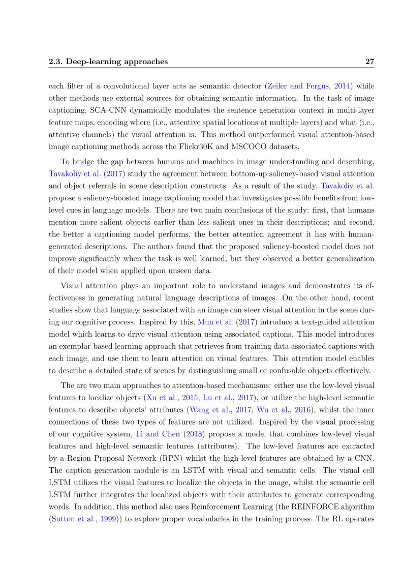
2.3. Deep-learning approaches 27

each filter of a convolutional layer acts as semantic detector (Zeiler and Fergus, 2014) whileother methods use external sources for obtaining semantic information. In the task of imagecaptioning, SCA-CNN dynamically modulates the sentence generation context in multi-layerfeature maps, encoding where (i.e., attentive spatial locations at multiple layers) and what (i.e.,attentive channels) the visual attention is. This method outperformed visual attention-basedimage captioning methods across the Flickr30K and MSCOCO datasets.

To bridge the gap between humans and machines in image understanding and describing,Tavakoliy et al. (2017) study the agreement between bottom-up saliency-based visual attentionand object referrals in scene description constructs. As a result of the study, Tavakoliy et al.propose a saliency-boosted image captioning model that investigates possible benefits from low-level cues in language models. There are two main conclusions of the study: first, that humansmention more salient objects earlier than less salient ones in their descriptions; and second,the better a captioning model performs, the better attention agreement it has with human-generated descriptions. The authors found that the proposed saliency-boosted model does notimprove significantly when the task is well learned, but they observed a better generalizationof their model when applied upon unseen data.

Visual attention plays an important role to understand images and demonstrates its ef-fectiveness in generating natural language descriptions of images. On the other hand, recentstudies show that language associated with an image can steer visual attention in the scene dur-ing our cognitive process. Inspired by this, Mun et al. (2017) introduce a text-guided attentionmodel which learns to drive visual attention using associated captions. This model introducesan exemplar-based learning approach that retrieves from training data associated captions witheach image, and use them to learn attention on visual features. This attention model enablesto describe a detailed state of scenes by distinguishing small or confusable objects effectively.

The are two main approaches to attention-based mechanisms: either use the low-level visualfeatures to localize objects (Xu et al., 2015; Lu et al., 2017), or utilize the high-level semanticfeatures to describe objects’ attributes (Wang et al., 2017; Wu et al., 2016), whilst the innerconnections of these two types of features are not utilized. Inspired by the visual processingof our cognitive system, Li and Chen (2018) propose a model that combines low-level visualfeatures and high-level semantic features (attributes). The low-level features are extractedby a Region Proposal Network (RPN) whilst the high-level features are obtained by a CNN.The caption generation module is an LSTM with visual and semantic cells. The visual cellLSTM utilizes the visual features to localize the objects in the image, whilst the semantic cellLSTM further integrates the localized objects with their attributes to generate correspondingwords. In addition, this method also uses Reinforcement Learning (the REINFORCE algorithm(Sutton et al., 1999)) to explore proper vocabularies in the training process. The RL operates

28 State of the Art

by introducing state perturbations to the LSTM units.

Top-down attention-mechanisms for building visual attention maps typically focus on someselective regions obtained from the output of one or two layers of a CNN. The input regionsare of the same size and have the same shape of the receptive field. Anderson et al. (2018b)argue that this approach has little consideration for the content of the image and propose a newmethod inspired by the human visual system. Recent studies on human attention (Buschmanand Miller, 2007) indicate that human attention can be focused volitionally by top-down signalsdetermined by the task at hand (e.g., looking for something), and automatically by bottom-up signals associated with unexpected, novel or salient stimuli. Inspired by these findings,Anderson et al. introduce a top-down mechanism based on Faster R-CNN Ren et al. (2015).This mechanism proposes image regions, each with an associated feature vector, while a top-down mechanism determines feature weightings. Therefore, this method can attend both objectlevel regions as well as other salient image regions.

Hao et al. (2018) propose another model based on the popular encoder-decoder architecture,but it uses the recently proposed densely convolutional neural network (DenseNet) to encode thefeature maps. Meanwhile, the decoder uses an LSTM to parse the feature maps and conversethem into textual descriptions. This model predicts the next word in the description by takingthe effective combination of feature maps with word embedding of current input word by avisual attention switch.

Khademi and Schulte (2018) present a context-aware attention-based method that employsa Bidirectional Grid LSTM (BiGrLSTM), which takes visual features of an image as inputand learns complex spatial patterns based on two-dimensional context, by selecting or ignoringits input. In addition, this method leverages a set of local region-grounded texts obtainedby transfer learning. The region-grounded texts often describe the properties of the objectsand their relationships in an image. To generate a global caption for the image, this methodintegrates the spatial features from the Grid LSTM with the local region-grounded texts, usinga two-layer Bidirectional Grid LSTM. The first layer models the global scene context such asobject presence. The second layer utilizes a dynamic spatial attention mechanism to generatethe global caption word-by-word while considering the caption context around a word in bothdirections. Unlike recent models that use a soft attention mechanism, this attention mechanismconsiders the spatial context of the image regions.

Jiang et al. (2018) propose an extension of the encoder-decoder framework by adding acomponent called guiding network. The guiding network models the attribute properties ofinput images, and its output is leveraged to compose the input of the decoder at each time step.The guiding network can be plugged into the current encoder-decoder framework and trainedin an end-to-end manner. Hence, the guiding vector can be adaptively learned according to the

2.3. Deep-learning approaches 29

signal from the decoder, making itself to embed information from both image and language.Additionally, discriminative supervision can be employed to further improve the quality ofguidance.

2.3.5 Compositional architectures

Most of the neural methods for image captioning described in the previous sections are end-to-end systems made of tightly coupled modules whose parameters are trained jointly. Analternative architectonic approach to build such systems is based on the notion of compositionalarchitectures, which consist of independent, loosely coupled components connected through apipeline, where each component provides data to the next component until a final result isobtained. The idea behind this architecture is to make modular systems where it is easier toreuse existing components and replace components with little effort.

The general structure of compositional image captioning methods is depicted in Fig. 2.4.Usually, there are three components:

1. A visual model that obtains visual features from the query image.

2. A natural language model that generates captions for the extracted features

3. A ranking module that re-ranks generated captions using a multimodal similarity model.

Figure 2.4: Structure of image captioning methods based on theencoder-decoder framework

Fang et al. (2015) describe a system that consists of three models: visual detectors, languagemodels and multimodal similarity models. The training process consists of two steps: First, avocabulary of words that are most common in the training captions. Second, a visual detectoris trained for each word in the vocabulary using multiple-instance learning (Viola et al., 2005).Once trained, the system can be used to generate image captions: A CNN (Krizhevsky et al.,2012) is used to obtain visual features expressed as words learned vocabulary, then a maxi-mum entropy language model (Berger et al., 1996) is applied to generate candidate captions

30 State of the Art

conditioned on those features. During this process, left-to-right beam search (Ratnaparkhi,2000) with a stack of pre-specified length l, produces l candidate descriptions. Finally, a deepmultimodal similarity model, which maps images and text fragments into a common space forsimilarity measurement, is used to re-rank the candidate descriptions and select the top one.

Taking on the same architecture introduced by Fang et al. (2015), Tran et al. (2016) presenta system specialized in describing landmarks and celebrities. However, instead of a CNN for thevisual feature detector, this model uses a deep residual network (ResNet) to detect a broaderrange of visual concepts He et al. (2016), a maximum entropy language model for candidatedescription generation, and a deep multimodal similarity model for caption ranking.

Ma and Han (2016) propose another method using a compositional architecture. Their maincontribution is the introduction of structural words; tetrads composed of <objects, attributes,activities, scenes>. The method consists of two stages: structural word generation and sentencetranslation. At the first stage, multi-layer optimization is applied to generate a hierarchy ofconcepts that will play the role of structural words. During the second stage, an LSTM is usedto translate the structural words into full sentences.

Realizing the high specialization of most approaches to multi-modal learning problems,Oruganti et al. (2016) introduce a more general approach called the Fusion-based RecurrentMulti-Modal (FRMM) model. This model is made of three independent components: one com-ponent per modality, and a fusion stage. Each modality is learned in a separate stage, and thentheir outputs are mapped to a shared representation. Finally, the fusion generates an outputbased on the associations between modalities it has previously learned. This approach pro-vides the FRMM architecture increased flexibility over previous approaches in accommodatingdisparate inputs. The architecture for each stage might be different depending on the modal-ities involved, ensuring that the overall architecture is highly adaptable. The FRMM modelis designed to work with multi-modal applications in which at least one of the modalities hasa temporal or sequential nature, such as image description, sentiment analysis, and languagetranslation. Furthermore, two variations of the FRMM architecture are proposed according tothe lengths of the inputs in each modality: Aligned FRMM (AFRMM) when the length is thesame, and Unaligned FRMMM (UFRMM) otherwise. For image captioning in particular, theAFRMM model achieved the best results. This models obtained better results for big datasetslike MSCOCO, but not for smaller datasets like Flickr30K, probably because it needs to learnmore parameters than other models.

Wang et al. (2016) propose a parallel version of the compositional architecture with thegoal of taking advantage of the complementary properties of simple RNNs one the one hand,and LSTMs networks on the other hand. There is a visual stage using CNN, like many otherapproaches, as well as a language generator and a fusion step. The contribution of this work

2.3. Deep-learning approaches 31

lies in the parallelization of the generation and fusion stages, which consists in dividing thehidden units of the RNN into several same-size parts and letting them work in parallel. Then,their outputs are merged with corresponding ratios for word prediction. This parallelizationallows for the use of different types of hidden units to combine their strengths. Specifically,the authors have used various configurations of simple RNN and LSTM. Experimental resultsshowed a reduction in resource consumption accompanied by a simultaneous improvement inperformance, compared with the dominated models (models using just one type of hidden units,either simple RNN or LSTM).

Gan et al. (2017b) introduce another compositional architecture based on the encoder-decoder framework. Their model, called Semantic Compositional Network (SCN) extractssemantic tags from the image, and the probability of each tag is used to compose the parametersin an LSTM network. The SCN extends each weight matrix of the LSTM to an ensemble oftag-dependent weight matrices. The degree to which each member of the ensemble is used togenerate an image caption is tied to the image-dependent probability of the corresponding tag.The same architecture can be used to describe video clips.

Fu et al. (2017) introduce an approach that aims at exploiting the parallel structures betweenimages and sentences. In this model, the generation of the next word is aligned with thevisual perception experience, where the attention shifting among the visual regions imposesa thread of visual ordering. In addition, this method uses high-level semantic informationin the form of scene-specific contexts. This method works as follows: First, selective search(Uijlings et al., 2013) is applied to construct a hierarchical segmentation of the image containingimage regions/patches at different scales. Second, a small number of regions are selected forfurther processing based on the criterion of being semantically meaningful, non-compositionaland contextually rich. Next, visual features are extracted from regions using a deep CNN.The sentence generation process is guided by an attention-based multi-modal LSTM decoder.The visual attention mechanism is inspired by the model described in (Xu et al., 2015), butit is enriched with information representing the scene-specific context. This information ismodeled as scene vectors obtained by Latent Dirichlet Allocation (LDA) (Blei et al., 2003) anda multilayer perceptron.

2.3.6 Other approaches

2.3.6.1 Language Convolutional Neural Networks

Since 2014, recurrent neural networks have been applied with great success to various sequencelearning tasks, including the image caption generation problem. Although traditional RNNssuffer from vanishing and exploding gradient problems and cannot adequately handle long-

32 State of the Art

term temporal dependencies, this problem is mitigated by modern architectures like LSTMHochreiter and Schmidhuber (1997) and GRU(Chung et al., 2014). Not surprisingly, thesenetwork architectures have also dominated the image captioning problem.

However, LSTM/GRUs ignore the underlying hierarchical structure of a sentence. They alsorequire significant storage due to long-term dependencies through a memory cell. In contrast,CNNs can learn the internal hierarchical structure of the sentences and they are faster inprocessing than LSTMs. Therefore, recently, convolutional architectures are being increasinglyused in sequence-to-sequence tasks, like conditional image generation and machine translation.Inspired the success of CNN in sequence learning tasks, some authors are proposing CNN as analternative to RNN for the language generation part of their image captioning methods. Theresult is a CNN+CNN alternative to the dominant CNN+RNN paradigm.

The first attempt to actually use CNN for the language model of an image captioning systemwas the multimodal convolutional neural network (m-CNN) proposed by Ma et al. (2015), thatwe already described as an earlier deep learning model.

More recently, Gu et al. (2017) introduce a language CNN model which is suitable forstatistical language modeling tasks and shows competitive performance in image captioning.In contrast to previous models which predict next word based on one previous word and hiddenstate, this language CNN is fed with all the previous words and can model the long-rangedependencies in history words, which are critical for image captioning. However, the methodcannot model the dynamic temporal behavior of the language model using just a language-CNN, thus it combines the language CNN with a recurrent network to model the temporaldependencies properly.

Aneja et al. (2018) propose a fully convolutional architecture (CNN+CNN) for the task ofimage captioning. This method uses a feed-forward network without any recurrent function.The architecture of the method has four components: (i) input embedding layer (ii) imageembedding layer (iii) convolutional module, and (iv) output embedding layer. It also usesan attention mechanism to leverage spatial image features. The evaluation on the MSCOCOdataset shows comparable performance to an LSTM based method on standard metrics

Wang and Chan (2018) also propose a CNN+CNN image captioning method. It is similar tothe method by Aneja et al., except that it includes a hierarchical attention module to connectthe vision-CNN with the language-CNN. The authors of this method also investigate the use ofvarious hyperparameters, including the number of layers and the kernel width of the language-CNN. They show how the influence of the hyperparameters can improve the performance ofthe method in image captioning.

2.3. Deep-learning approaches 33

2.3.6.2 Reinforcement Learning

Most image captioning methods are trained by maximizing the likelihood of ground-truth an-notated captions given the image. While simple and easy to implement, this approach does notdirectly maximize language quality metrics such as CIDEr. In order to improve on this kindof metrics, recently proposed methods include some form of Reinforcement Learning as a wayto improve the quality of generated captions with respect to this kind of metric. However, RLfaces various problems when applied to language generation problems. First, unlike images,which are represented using real numbers, text processing is based on discrete numbers, whichresults in non-differentiable functions, making it difficult to apply back-propagation directly.However, this problem can be overcome by using the REINFORCE family of algorithms, whichintroduces Policy gradient with differentiable function approximation (Sutton et al., 1999).

Rennie et al. (2017) propose a new optimization approach called self-critical sequence train-ing (SCST). SCST is a form of the popular REINFORCE algorithm that, rather than estimatinga base-line to normalize the rewards and reduce variance, utilizes the output of its own test-timeinference algorithm to normalize the rewards it experiences. Using this approach, estimatingthe reward signal (as actor-critic methods must do) and estimating normalization (as REIN-FORCE algorithms typically do) is avoided, while at the same time harmonizing the modelwith respect to its test-time inference procedure. Empirically, the authors find that directlyoptimizing the CIDEr metric with SCST and greedy decoding at test-time is highly effective.

The method proposed by Li and Chen (2018) also includes a REINFORCE algorithm toimprove their captions by optimizing the CIDEr metric. This method is described in the sectiondevoted to attention-based methods, so it is not described here again..

Zhang et al. (2017) investigate an actor-critic reinforcement learning (Barto et al., 1983)approach. The architecture of this method consists of a policy network (actor) and a valuenetwork (critic). The actor treats the job as a sequential decision problem and can predictthe next token of the sequence. In each state of the sequence, the network will receive itsevaluation metrics score as a reward. The job of the critic is to predict the reward. If itcan predict the expected reward, the actor will continue to sample outputs according to itsprobability distribution.

The existing image captioning approaches typically train a one-stage sentence decoder,which makes it difficult to produce fine-grained descriptions. On the other hand, multi-stagesentence decoders are hard to train due to the vanishing gradient problem. Gu et al. (2018)propose a coarse-to-fine multi-stage decoder composed of a number of stacked decoders eachof which operates on the output of the previous stage, producing increasingly refined imagedescriptions. The vanishing gradient problem is tackled by providing a learning objectivefunction that enforces intermediate supervisions. In particular, the model is optimized with a

34 State of the Art

reinforcement learning method which utilizes the output of each intermediate decoder’s test-time inference algorithm as well as the output of its preceding decoder to normalize the rewards.This method also solves the exposure bias problem and the loss-evaluation mismatch problem.

2.3.6.3 Generative Adversarial Networks

Despite phenomenal research progresses in the past several years, sentences produced by meth-ods based on Recurrent Neural Networks tend to be rigid and lacking in variability becausethey learn by maximizing the likelihood of ground-truth annotated captions in the training ex-amples. This principle encourages high resemblance to the ground-truth captions, thus missingthe opportunity to generate other reasonable descriptions. Conventional evaluation metrics,e.g. BLEU and METEOR, also favor such restrictive methods.

Generative Adversarial Networks (GAN) provides a possible way to generate more diverseand distinctive captions. GANs can learn deep features from unlabeled data. They achieve theserepresentations applying a competitive process between a pair of networks: the Generator andthe Discriminator.

Dai et al. (2017) introduce a method based on GAN with the aim to improve the naturalnessand diversity of generated captions. This method, called Conditional GAN (CGAN), jointlylearns a generator to produce descriptions conditioned on images, and an evaluator to assesshow well a description fits the visual content. GANs face two problems when compared withRNN. First, like Reinforcement Learning, it is difficult to apply back-propagation directly,but similarly, this problem can be tackled by introducing policy gradient mechanism withdifferentiable function approximation (Sutton et al., 1999). Second, sequence generation facesvanishing gradients and error propagation training difficulties. A way to mitigate this problemis to provide early feedback to the mitigator. Following this idea, CGAN adds Monte Carlorollouts to compute future reward values at early stages of the process (Yu et al., 2017). Thismethod only generates one caption per image.

Shetty et al. (2017) introduce another GAN based method that is able to generate multiplecaptions for a single image. Instead of function approximation used by other methods todeal with the discrete data backpropagation problem, this method uses Gumbel sampler (Janget al., 2017). During training, the generator learns the loss value provided by the discriminatorinstead of learning it from explicit sources. The discriminator has true data distribution andcan discriminate between generator-generated samples and true data samples. This allowsthe network to learn diverse data distribution. Moreover, the network classifies the generatedcaption sets into either real or fake.

Li et al. (2018) propose a conditional GAN for generating diverse captions across images.Instead of estimating the quality of a caption solely on one image, the proposed comparative

2.3. Deep-learning approaches 35

adversarial learning framework assesses the quality of captions by comparing a set of captionswithin the image-caption joint space. The proposed architecture, called Comparative Adver-sarial Learning (CAL) Network consists of a caption generator and a comparative relevancediscriminator which play a min-max game and optimize the loss function. With the guidesfrom the discriminator, the generator effectively learns to generate more specific and distinc-tive captions, hence increases the diversity across the corpus.

2.3.6.4 Other methods

The majority of methods described in former sections are variations of the encoder-decoderframework following the CNN+RNN schema, that is to say, the encoder uses ConvolutionalNeural Networks Lecun et al. (1998), and the decoder uses Recurrent Neural Networks, suchas LSTM(Hochreiter and Schmidhuber, 1997) or GRU(Chung et al., 2014).

There is also a new wave of models that replace the RNN encoder module with some formof CNN for language modeling (CNN+CNN methods) or variants of the Generative AdversarialTraining, but in general, all these methods still rely on a single CNN for the encoder layer.That is, the CNN feature map of the image is taken as the source input to the decoder module.

An exception to the standard CNN+RNN approach is the model proposed by Liu et al.(2017b), called MAT, which stands for Multimodal Attentive Translator. The main idea behindMAT is to view the image captioning problem as a specific form of translation task, from asequence of objects into a sequence of words. To that aim, instead of modeling the input imageas a feature map, as most CNN-based approached do, the input image has to be representedas a sequence of detected objects. In order to model the image as a sequence, MAT introducesa sequential attention layer to selectively attend to the objects that are related in order togenerate corresponding words. Here, the input layer expands the image representation from asingle CNN at a single time step in RNN, to a sequence of objects at multiple time steps. Thisarchitecture combines CNN object detectors with LSTM for the encoding module, a secondLSTM for the decoding module, plus an attention module.

The majority of deep learning approaches to the image captioning problem take the super-vised learning route, with some exceptions that use some form of semi-supervised learning(Puet al., 2016a; Anderson et al., 2018a). However, Feng et al. (2018) propose a completely un-supervised approach to training an image captioning model. Instead of relying on manuallylabeled image-sentence pairs, this method merely requires an image set, a sentence corpus,and an existing visual concept detector. The sentence corpus is used to teach the languagegeneration model how to generate plausible sentences. Meanwhile, the knowledge in the visualconcept detector is distilled into the captioning model to guide the model to recognize the visualconcepts in an image. Furthermore, the image and caption are projected into a common latent

36 State of the Art

space so that they can reconstruct each other. Given that the existing sentence corpora aremainly designed for linguistic research, the authors have also crawled a large-scale image de-scription corpus of two million natural sentences to facilitate the unsupervised image captioningscenario. Experimental results show promising results without any caption annotations.

Lindh et al. (2018) also introduce a form of unsupervised learning, although their model stillrelies on supervised learning for the most part. These authors address the low diversity andspecificity in generated sentences that limit many image captioning methods by introducing anImage Retrieval model to improve the caption specificity of the Image Captioning model. Thismodel uses the error signal from the Image Retrieval model to improve caption specificity, whichis expected to increase diversity. Training is inspired by GAN: the discriminator is replaced bythe Image Retrieval module, and the generator is replaced by the Image Captioning module.But, unlike GAN, where the generator and discriminator learn from each other, in this methodthe discriminator is pre-trained and doesn’t learn from the generator.

2.3.6.5 Describing novel objects

The image captioning methods described so far are limited to predefined vocabularies, that is,these methods are unable to generate descriptions for novel objects, objects that are not asso-ciated to any of the concepts represented in the training data (image-sentence pairs). However,humans have the ability to recognize, learn and use novel concepts in various visual under-standing tasks. In practical image description applications, it is quite possible to come acrosssituations where there are novel objects which are not included in the vocabulary learned bythe model and would be very costly to retrain the system every time a new concept appears.In this section, we describe some attempts to deal with novelties in image captioning.

In order to learn novel visual concepts without retraining the whole system, Mao et al. (2015)propose a method that uses just a few images with sentence descriptions. This method is able tohypothesize the semantic meaning of new words and add them to its dictionary for future use.In order to implement and test this method, the authors have modified their previous model(Mao and Yuille, 2015) to make it more suitable for the novel concept learning task. On theone hand, a transposed weight sharing strategy is applied to reduce the number of parameters,which in turn makes the model less prone to overfitting the new concepts. Second, an LSTMnetwork replaces the simple RNN to avoid the gradient explosion and vanishing problem.

Another approach to make image captioning capable of describing novel objects is the DeepCompositional Captioner (DCC), by Hendricks et al. (2016). The DCC achieves this goalby leveraging large object recognition datasets and external text corpora, and by transferringknowledge between semantically similar concepts. First, a lexical classifier and a languagemodel are trained over image datasets and text corpora, respectively. Then, a multimodal

2.4. Datasets and evaluation 37

caption model is trained to integrate the lexical classifier and the language model using linearcombinations of affine transformations of image and language features. This model enables thetransfer of semantic knowledge between the two modalities, which allows generating descriptionsfor novel objects and their interactions with other objects.

2.4 Datasets and evaluation

There is a wide range of datasets available for automatic image captioning research. The imagesin these datasets are linked to textual captions and differ from each other in certain aspectssuch as in size, the format of the captions, or the procedure used to collect the data. Thissection presents a brief overview of the common approaches used to collect data, the datasetsthemselves, and the metrics utilized for model evaluation and benchmarking.

The datasets are summarized in Table 2.3, and examples of images their correspondingcaptions are given in Fig. 2.5. For a wider survey of datasets in the CV and NLP fields thereader is referred to Ferraro et al. (2015). That survey is not limited to image captioning andprovides additional statistics and quality metrics such as perplexity, syntactic complexity, andabstract to concrete word ratios.

Some authors establish a difference between image captions and image descriptions, andin this survey, we have actually used them interchangeably. However, such a distinction isrelevant when presenting datasets. Image descriptions verbalize what can be seen in the image,i.e., they refer to the objects, actions, and attributes depicted, etc. Captions, on the otherhand, typically provide information that cannot be seen in the image or is not evident, suchas personal, cultural, or historical context. Images shared through social networks or photo-sharing websites can be accompanied by descriptions or captions, or a mixture of both typesof text. The images in a newspaper or a museum will typically contain cultural or historicaltexts, i.e., captions not

2.4.1 Datasets

This subsection briefly describes the most popular datasets used in image description tasks,sorted by year of publication.

The Pascal1K sentence dataset Rashtchian et al. (2010) consists of 1000 images that wereselected from the Pascal 2008 object recognition dataset2 (Everingham et al., 2010). The

2Every year, the Pattern Analysis, Statistical Modeling, and Computational Learning (PASCAL) organiza-tion hosts the Visual Object Classes Challenge. In this competition, a new dataset of images with classificationand detection information is released, and computer vision researchers compete to create the best classification,detection, and segmentation systems

38 State of the Art

Table 2.3: Summary of benchmark datasets.

Dataset Images Texts Judgements Objects

Pascal1K (Rashtchian et al., 2010) 1K 5 No PartialIAPTR-TC12 (Escalante et al., 2010) 20K 1-5 No SegmentedVLT2K (Elliott and Keller, 2013) 2K 3 Partial PartialFlickr8K (Rashtchian et al., 2010) 8K 5 Yes NoAbstract Scenes (Zitnick et al., 2013) 10K 6 No CompleteFlickr30K (Young et al., 2014) 31K 5 No NoMSCOCO (Lin et al., 2014) 328K 5 Collected PartialConceptual Captions (Sharma et al., 2018) 3.3M 1 No No

dataset covers a wide variety of objects and scenery classified into 20 different categories, suchas humans, animals, and vehicles. Each image is associated with five one-sentence descriptionsgenerated by humans using the Amazon Mechanical Turk (AMT)3 crowdsourcing service.For the image annotation process, the Turkers (AMT workers) were instructed to focus on theimages and describe their contents without considering the context.

The IAPR-TC12 dataset (Escalante et al., 2010) contains an image collection consistingof 20k images taken from locations around the world and comprising a varying cross-sectionof still natural images. They were obtained by guides of an independent travel company andundergo a selection process. The images are accompanied by written descriptions expressed inmultiple languages (predominantly English and German). Each image is associated with oneto five descriptions, sorted by a certain priority pattern.

The Visual and Linguistic Treebank (VLT) (Elliott and Keller, 2013) makes use ofimages from the Pascal 2010 action recognition dataset, augmented with three descriptions oftwo sentences length per image. These descriptions were collected on the AMT with specificinstructions to verbalize the main action depicted in the image and the actors involved (firstsentence), as well as the most important background objects (second sentence). There areobject annotations available for a subset of 341 images, in the form of polygons around allobjects mentioned in the descriptions. Moreover, this subset also includes 3 manually-createdVisual Dependency Representations (VDR) per image.

The Flickr8K dataset (Rashtchian et al., 2010) comprises approximately 8k images ob-tained from the Flickr photo-sharing website. The images in this dataset were collected throughuser queries for specific objects and actions using the AMT. The descriptions consist of 5 sen-tences per image collected from AMT workers using a strategy similar to that of the Pascal1K

3Amazon Mechanical Turk (MTurk) is a crowdsourcing marketplace that makes it easier for individuals andbusinesses to outsource their processes and jobs to a distributed workforce who can perform these tasks virtually.This could include anything from conducting simple data validation and research to more subjective tasks likesurvey participation, content moderation, and more. See https://www.mturk.com/

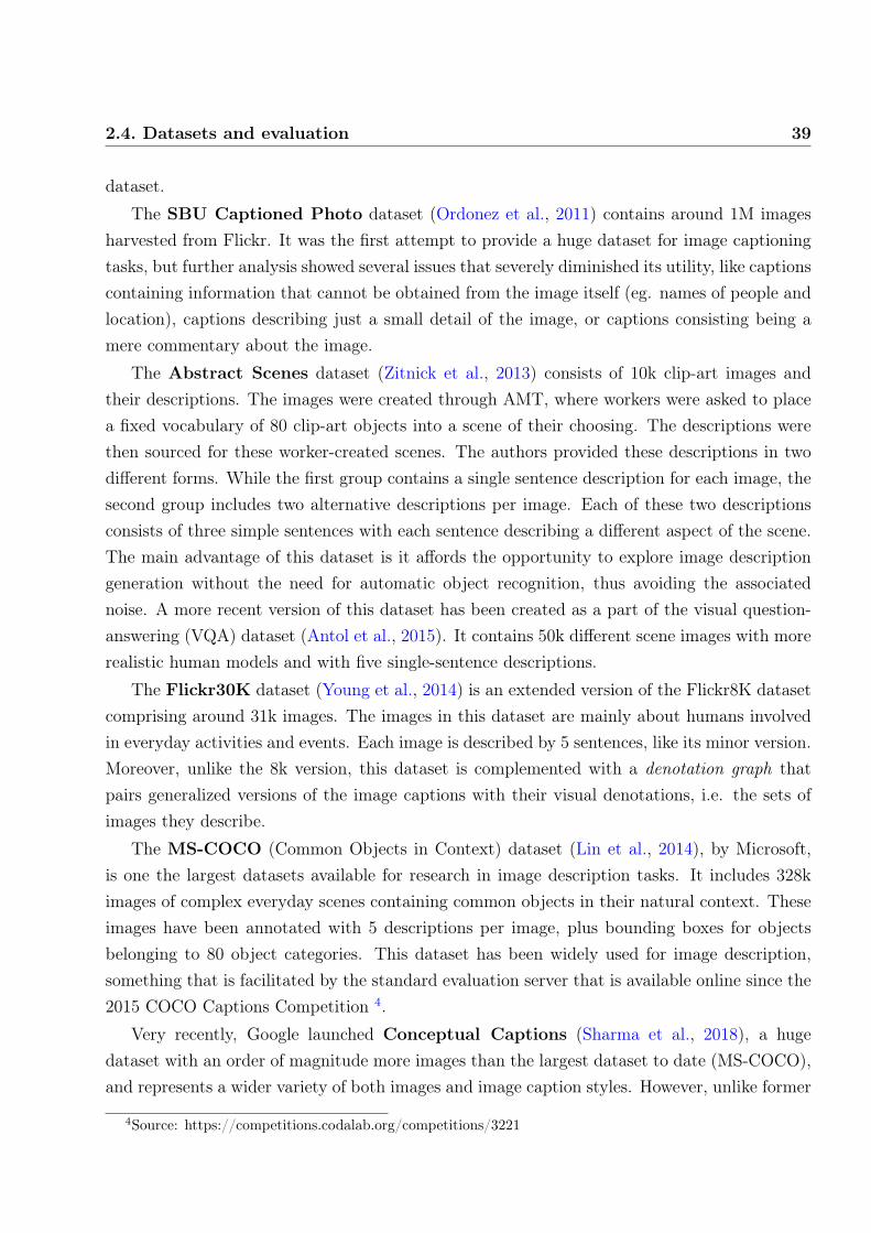
2.4. Datasets and evaluation 39

dataset.

The SBU Captioned Photo dataset (Ordonez et al., 2011) contains around 1M imagesharvested from Flickr. It was the first attempt to provide a huge dataset for image captioningtasks, but further analysis showed several issues that severely diminished its utility, like captionscontaining information that cannot be obtained from the image itself (eg. names of people andlocation), captions describing just a small detail of the image, or captions consisting being amere commentary about the image.

The Abstract Scenes dataset (Zitnick et al., 2013) consists of 10k clip-art images andtheir descriptions. The images were created through AMT, where workers were asked to placea fixed vocabulary of 80 clip-art objects into a scene of their choosing. The descriptions werethen sourced for these worker-created scenes. The authors provided these descriptions in twodifferent forms. While the first group contains a single sentence description for each image, thesecond group includes two alternative descriptions per image. Each of these two descriptionsconsists of three simple sentences with each sentence describing a different aspect of the scene.The main advantage of this dataset is it affords the opportunity to explore image descriptiongeneration without the need for automatic object recognition, thus avoiding the associatednoise. A more recent version of this dataset has been created as a part of the visual question-answering (VQA) dataset (Antol et al., 2015). It contains 50k different scene images with morerealistic human models and with five single-sentence descriptions.

The Flickr30K dataset (Young et al., 2014) is an extended version of the Flickr8K datasetcomprising around 31k images. The images in this dataset are mainly about humans involvedin everyday activities and events. Each image is described by 5 sentences, like its minor version.Moreover, unlike the 8k version, this dataset is complemented with a denotation graph thatpairs generalized versions of the image captions with their visual denotations, i.e. the sets ofimages they describe.

The MS-COCO (Common Objects in Context) dataset (Lin et al., 2014), by Microsoft,is one the largest datasets available for research in image description tasks. It includes 328kimages of complex everyday scenes containing common objects in their natural context. Theseimages have been annotated with 5 descriptions per image, plus bounding boxes for objectsbelonging to 80 object categories. This dataset has been widely used for image description,something that is facilitated by the standard evaluation server that is available online since the2015 COCO Captions Competition 4.

Very recently, Google launched Conceptual Captions (Sharma et al., 2018), a hugedataset with an order of magnitude more images than the largest dataset to date (MS-COCO),and represents a wider variety of both images and image caption styles. However, unlike former

4Source: https://competitions.codalab.org/competitions/3221

40 State of the Art

datasets, which were annotated manually by humans, the 3.3M images of this dataset were col-lected programmatically, by extracting and filtering images and text annotations from billionsof webpages. It consists of a wide variety of images and associated descriptions taken from orig-inal Alt-text attributes, automatically transformed to achieve a balance between cleanliness,informativeness, and learnability. The remaining image, caption pairs contain around 16,000entity types, guaranteed to be well represented in terms of the number of examples.

2.4.1.1 Other datasets

This subsection summarizes other datasets that, in spite of being less popular than the onesalready presented, are to a certain extent relevant to the problem at hand.

• The Attribute Discovery dataset (Berg et al., 2010) was collected using automatic datasetconstruction techniques that exploit the connection between text and images. Thisdataset consists of 4 broad shopping categories (bags, earrings, ties, and shoes). Thedata set was collected from like.com and includes both images and associated textualdescriptions.

• The MIT-Adobe FiveK (Bychkovsky et al., 2011) dataset consists of 5K images con-taining a diverse set of scenes, subjects, and lighting conditions. These images are mainlyabout people, nature, and man-made objects.

• The NYU-v2 dataset (Silberman et al., 2012) is a more specialized dataset containing1.5K RGBD images capturing 464 diverse indoor scenes, with detailed annotations. Theparticularity of this dataset is its focus on 3D segmentation. It has been augmented withfive descriptions per image by Lin et al. (2015) for image description tasks.

• The SUN Attribute database (Patterson et al., 2014) provides around 15K images from707 scene categories. It was derived from the SUN categorical database using crowdsourc-ing to annotate images with attributes. Previously, crowdsourced human studies wereconducted to find a taxonomy of 102 discriminative attributes related to varied aspects,such as materials, surface properties, lighting, affordances, and spatial layout.

• The FlickrStyle10k dataset has 10K Flickr images with stylized captions. The trainingdata consists of 7K images. The validation and test data consist of 2,000 and 1,000 imagesrespectively. Each image contains romantic, humorous, and factual captions.

• The Stock3M dataset (Wang et al., 2017) has more than 3M images uploaded by theusers of a stock image website. Each image is associated with one caption that is providedby the photo uploader. The captions are much shorter than those found on the MSCOCO

2.4. Datasets and evaluation 41

Figure 2.5: Examples of images and their descriptions across variousbenchmark datasets

42 State of the Art

dataset but are claimed to be more natural, with a larger vocabulary and image contentvariety.

• The VQA (Visual Question Answering) dataset is intended to support a variation of theimage description problem called visual question answering : given an image and a naturallanguage question about the image, the task is to provide an accurate natural languageanswer (Antol et al., 2015). To that aim, the dataset contains 50K abstract scenes usingclip-art style graphics. It includes 20 paper-doll human models spanning genders, races,and ages with 8 different expressions, over 100 objects and 31 animals in various poses.The images are completed with five captions per image, as well as diverse questions andanswers.

2.4.2 Evaluation metrics

Evaluating Natural Language Generation (NLG) systems is a fundamentally difficult task (Re-iter and Belz, 2009) so that it has become a research problem itself. However, we will simplysummarize the metrics commonly used for evaluating the quality of image descriptions gener-ated automatically.

2.4.2.1 Human judgement

A common way to assess the quality of automatically generated texts is Subjective evaluation byhuman judges. Automatically produced text is usually judged in terms of syntactical correctness(grammar compliance) and semantic correctness (relevance of the content). Another dimensionof interest is the fluency of the text, especially when a surface realization technique is involvedin the generation process. Image descriptions generated automatically can be evaluated usingthe same techniques that are common in other NLG tasks, an very particularly in machinetranslation (MT) tasks. In this case, judges get both the image and the generated descriptionfor the evaluation task. Subjective human evaluations of machine-generated image descriptionsare often performed on the Amazon Mechanical Turk by means of Likert-scale questions. Someexamples of these kinds of questions are:

• The description accurately describes the image

• The description is grammatically correct

• The description has no incorrect information

• The description is relevant for this image

• The description is human like

2.4. Datasets and evaluation 43

2.4.2.2 Automatic evaluation metrics

Since human evaluation requires large amounts of non-reusable human effort, it is difficult toscale up. Furthermore, human judgment is inherently subjective, which makes it suffer fromuser variances. To avoid these pitfalls, automated metrics have been created with differentproperties. Below follows a short review of the most common metrics used for evaluatingmachine-generated image descriptions.

Classical information retrieval metrics, like the median rank (mRank) and the precisionand recall at k (S@k, R@K) have been included quite often to evaluate the descriptions returnedby image captioning methods, particularly with for methods that adopt an information retrievalapproach, although they are not considered the most appropriate metric for this task.

IBM’s BLEU (Bilingual Evaluation Understudy) (Papineni et al., 2002) is a family ofmetrics conceived to substitute human judges in the evaluation of MT tasks, so besides beingquick, inexpensive and language independent, it was designed to show good correlation withhuman judgment. This family of metrics uses a weighted average of variable length phrasematches against the reference translations written by humans to measure their closeness. BLEUstarts with a baseline metric from which a number of metrics are derived for different n-gramsizes: BLEU-1 compares the candidate sentence with sentences in unigram, BLEU-2 comparesthe candidate sentence with sentences in bigram, and so on, until BELU-4, which obtainsthe best correlation with human judgments. While unigram scores account for the adequacy,higher n-gram scores account for fluency. BLEU is popular because was it was the first metricpopularized for MT tasks, long before the research on automatic image generation field tookoff. Although BLEU shows a reasonable correlation with human judgments it seems to workwell only when the generated text is sort (Callison-Burch et al., 2006), and it may even occurthat an increase in BLEU score did not correspond to an increase of quality (Lin and Och,2004).

ROUGE (Recall-Oriented Understudy for Gisting Evaluation) (Lin, 2004) is a set of met-rics introduced as an alternative to BLEU to work with larger texts, like text summaries.This metric employs the longest common subsequence between a candidate sentence and aset of reference sentences to measure their similarity at sentence-level. The longest commonsubsequence between two sentences only requires in-sequence word matches, and the matchedwords are not necessarily consecutive. Determination of the longest common subsequence isachieved by using dynamic programming. Different versions of ROUGE exist for different tasks:ROUGE-1 and ROUGE-W are appropriate for single document evaluation whereas ROUGE-2and ROUGE-SU4 have good performance for short summaries.

METEOR (Metric for Evaluation of Translation with Explicit ORdering) (Banerjee andLavie, 2005) is another metric originally conceived to evaluate MT tasks. It is based on

44 State of the Art

a generalized concept of unigram matching between the machine- produced translation andhuman-produced reference translations. Unigrams can be matched based on their surface forms,stemmed forms, and meanings. It first performs generalized unigram matches between a can-didate sentence and a human-written reference sentence and then computes a score based onthe matching results. The score computation involves precision, recall, and alignments of thematched elements, and in the case of multiple reference sentences, the best score among all thepossible matches is taken as the final evaluation score. METEOR achieves better correlation atthe sentence or the segment levels. There exists a Universal version of this metric supportingmany languages, like Russian and Hindi Denkowski and Lavie (2014).

CIDEr (Consensus-based Image Description Evaluation) (Vedantam et al., 2015) adoptsa novel paradigm which is based on human consensus and was designed specifically to eval-uate image description tasks instead of MT tasks. This metric measures the similarity of anautomatically generated sentence to the majority –consensus– of ground-truth sentences (im-age descriptions) written by humans. It works by encoding the frequency of the n-grams inthe candidate sentence that appear in the reference sentences using a Term Frequency-InverseDocument Frequency (TF-IDF) weighting for each n-gram. While most existing datasets haveonly five captions per image, which the authors consider is not enough to use human con-sensus, therefore they also created two new datasets with 50 human-generated sentences perimage: Pascal-50S and Abstract-50S, which uses the 1000 images from the Pascal1K, and500 random images from the Abstract Scene dataset, respectively. A version of CIDEr namedCIDEr-D is available as a part of the MSCOCO evaluation server to enable systematic eval-uation and benchmarking.

SPICE (Semantic Propositional Image Caption Evaluation) (Anderson et al., 2016) is anew evaluation metric for image descriptions based on a graph-based semantic representationof images called scene-graph (Johnson et al., 2015; Schuster et al., 2015). This graph canextract the information of different objects, attributes and their relationships from the imagedescriptions, and is based on the assumption that semantic propositional content is an impor-tant component of human caption evaluation. Extensive evaluations across a range of modelsand datasets indicate that SPICE captures human judgments over model-generated captionsbetter than other automatic metrics. Furthermore, SPICE can answer questions such as whichcaption-generator best understands colors? and can caption-generators count?

SPIDEr Liu et al. (2017c) has been proposed recently to overcome some of the problemsattributed to existing metrics by combining the properties of two of them: CIDEr and SPICE.This combination is achieved by means of a policy gradient (PG) method that directly op-timizes a linear combination of SPICE and CIDEr (hence the name SPIDEr). SPICE scoreensures semantic faithfulness of generated sentences, while CIDEr score guarantees that these

2.4. Datasets and evaluation 45

descriptions are syntactically fluent.(Sharif et al., 2018) explore a learning-based approach to combine various metrics and

report on their results. The idea behind this metric is the same behind SPIDEr: while somemetrics tend to focus on the lexical and syntactical correctness (BLEU, ROUGE, CIDEr), othermetrics tend to focus on the semantic relevance (SPICE). Therefore, combining the linguisticproperties of various metrics should help achieve a better assessment of the quality of imagedescription. Experimental results show improvements over other metrics in terms of correlationand accuracy on the Pascal-50S dataset.

2.4.3 Summary of methods, datasets, metrics and benchmark results

This subsection summarises all the published research covered in this survey. We begin withan extended overview of the reviewed methods for image captioning that use deep learningtechniques. We already presented an overview of methods in Table 2.1, but this time weinclude additional information to classify and characterize the methods. This information isdescribed below, and it is presented in Table 2.4.

• The network architecture used to encode images. All methods use convolutional neuralnetworks (CNN), but they differ in the specific network architecture, like VGG, Inceptionor ResNet, among others.

• The kind of network used to learn the language model, typically some form of LSTM,but also other RNN and other models.

• A classification of the method across multiple dimensions.

– Visual Space (VS) vsMultimodal Space (MS): Most methods model the imagein the visual space, but some methods learn a combined visual and language space(see §2.3.2)

– Supervised Learning (SL) vs Other Deep Learning (ODL). Although mostmethods use supervised learning, in some cases a form of semisupervised or un-supervised learning is employed (eg. generative adversarial networks (GAN) andreinforcement learning (RL)).

– Whole Scene (WS) vs Dense Captioning (DC): Most methods encode anddescribe images treated as a whole, but some approaches also detect regions in theimage and generate descriptions for those regions.

– Encode-Decoder (EDA) vs Compositional Architecture (CA): many ap-proaches adopt and encode-decoder architecture (see §2.3.3), while only a few ap-proaches adopt a compositional architecture (see §2.3.5).

46 State of the Art

• In addition to the above dimensions, some methods are annotated with extra descriptorsto further characterize the image captioning methods:

– Attention-Based (AB) refers to methods that can dynamically focus on variousparts of the image while the language descriptions are generated (see §2.3.4).

– Semantic Concept-Based (SCB) methods selectively attend to a set of semanticconcepts extracted from the image, so these methods apply a very specific form ofattention mechanism.

– Novel Object (NOB) is used to characterize those methods that are able to de-scribe objects that were not learned, that is, objects that were not included in thetraining dataset (see §2.3.6.5).

– Stylized Captions (SC) refers to the use of styles (eg. romantic, humorous) togenerate more attractive captions.

Other acronyms used in this classification are:

• LBL: Log-Bilinear Language Model. It is a neural language model that operates on a fea-ture vector representation of words. Word embeddings are computed using a feedforwardneural network. Then, the probability of the next word is computed given the previouswords (context) (see (Mnih and Hinton, 2007) for details).

• SC-NLM: Structure-Content Neural Language Model. It is a multimodal neural languagemodel proposed by (Kiros et al., 2014a)

• DTR: Dependency Tree Relations Structure that represents all sentence relationshipsuniformly as typed dependency relations, that is, as triplets of a relation between pairsof words (see (De Marneffe et al., 2006)).

• MELM: Maximum Entropy Language Model. This model predicts the next word in asentence based on the principle of maximum entropy (see (Berger et al., 1996) for details).

• HM-LSTM: Hierarchical Multimodal LSTM. Variation of the LSTM architecture pro-posed by Niu et al. (2017)

• LCNN: Language CNN. Refers to the use of convolutional neural networks to representlanguage models 5.

5The use of CNNs for sentence modeling traces back to Collobert and Weston (2008). The ability of CNNsto create informative latent semantic representations of sentences for downstream tasks Collobert et al. (2011);Kalchbrenner et al. (2014); Kim (2014) led to a huge proliferation of CNN-based networks applied to NLP tasks.

2.4. Datasets and evaluation 47

Note: In the classification presented in Table 2.4, we have omitted various methods describedin the earlier works section (§2.3.1) that do not fit in the proposed dimensions. These methodsare Socher et al. (2014); Lebret et al. (2015a,b); Yagcioglu et al. (2015).

Table 2.4: Classification of deep-learning methods

Publication Image Encoder Language Model Category

Karpathy et al. (2014) AlexNet DTR MS,SL,WS,EDAKiros et al. (2014a) AlexNet LBL MS,SL,WS,EDAKiros et al. (2014b) AlexNet, VGG LSTM,SC-NLM MS,SL,WS,EDAMao et al. (2014) AlexNet RNN MS,SL,WSChen and Zitnick (2015) VGG RNN VS,SL,WS,EDADonahue et al. (2015) Caffe LSTM VS,SL,WS,EDADevlin et al. (2015) VGG MELM MS,SL,SL,WS,EDAFang et al. (2015) AlexNet,VGG MELM VS,SL,WS,EDAJia et al. (2015) VGG LSTM VS,SL,WS,CA, SCBKarpathy and Fei-Fei (2015) VGG RNN MS,SL,WS,EDAMa et al. (2015) VGG LCNN MS,SL,WS,EDAMao and Yuille (2015) AlexNet,VGG RNN MS,SL,WSVinyals et al. (2015) Inception-V1 LSTM VS,SL,WS,EDAXu et al. (2015) AlexNet LSTM VS,SL,WS,EDA,ABHendricks et al. (2016) VGG LSTM VS,SL,WS,CA,NOBJohnson et al. (2016) VGG LSTM VS,SL,DC,EDAMa and Han (2016) AlexNet LSTM VS,SL,WS,CAMao et al. (2016) AlexNet,VGG LSTM VS,SL,WS,EDAMathews et al. (2016) Inception-V1 LSTM VS,SL,WS,EDA,SCSugano and Bulling (2016) VGG LSTM VS,SL,WS,EDA,ABTran et al. (2016) ResNet MELM VS,SL,WS,CAWang et al. (2016) VGG LSTM VS,SL,WS,CAWu et al. (2016) VGG LSTM VS,SL,WS,EDA,SCBYang et al. (2016) VGG LSTM VS,SL,DC,EDA,ABYou et al. (2016) Inception-V1 RNN VS,SL,WS,EDA,SCBChen et al. (2017a) VGG,ResNet LSTM VS,SL,EDA,ABDai et al. (2017) VGG LSTM VS,ODL,WS,EDAFu et al. (2017) VGG LSTM VS,SL,WS,EDA,ABGan et al. (2017a) ResNet LSTM VS,SL,WS,EDA,SCGan et al. (2017b) ResNet LSTM VS,SL,WS,CA,SCB

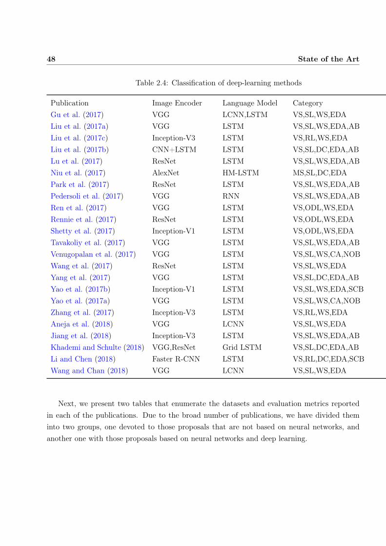
48 State of the Art

Table 2.4: Classification of deep-learning methods

Publication Image Encoder Language Model CategoryGu et al. (2017) VGG LCNN,LSTM VS,SL,WS,EDALiu et al. (2017a) VGG LSTM VS,SL,WS,EDA,ABLiu et al. (2017c) Inception-V3 LSTM VS,RL,WS,EDALiu et al. (2017b) CNN+LSTM LSTM VS,SL,DC,EDA,ABLu et al. (2017) ResNet LSTM VS,SL,WS,EDA,ABNiu et al. (2017) AlexNet HM-LSTM MS,SL,DC,EDAPark et al. (2017) ResNet LSTM VS,SL,WS,EDA,ABPedersoli et al. (2017) VGG RNN VS,SL,WS,EDA,ABRen et al. (2017) VGG LSTM VS,ODL,WS,EDARennie et al. (2017) ResNet LSTM VS,ODL,WS,EDAShetty et al. (2017) Inception-V1 LSTM VS,ODL,WS,EDATavakoliy et al. (2017) VGG LSTM VS,SL,WS,EDA,ABVenugopalan et al. (2017) VGG LSTM VS,SL,WS,CA,NOBWang et al. (2017) ResNet LSTM VS,SL,WS,EDAYang et al. (2017) VGG LSTM VS,SL,DC,EDA,ABYao et al. (2017b) Inception-V1 LSTM VS,SL,WS,EDA,SCBYao et al. (2017a) VGG LSTM VS,SL,WS,CA,NOBZhang et al. (2017) Inception-V3 LSTM VS,RL,WS,EDAAneja et al. (2018) VGG LCNN VS,SL,WS,EDAJiang et al. (2018) Inception-V3 LSTM VS,SL,WS,EDA,ABKhademi and Schulte (2018) VGG,ResNet Grid LSTM VS,SL,DC,EDA,ABLi and Chen (2018) Faster R-CNN LSTM VS,RL,DC,EDA,SCBWang and Chan (2018) VGG LCNN VS,SL,WS,EDA

Next, we present two tables that enumerate the datasets and evaluation metrics reportedin each of the publications. Due to the broad number of publications, we have divided theminto two groups, one devoted to those proposals that are not based on neural networks, andanother one with those proposals based on neural networks and deep learning.

2.4. Datasets and evaluation 49

Table 2.5: Summary of non neural methods, datasets and evaluationmetrics.

Publication Datasets Evaluation Metrics

Farhadi et al. (2010) Pascal1K BLEUKulkarni et al. (2011) Pascal1K Human, BLEULi et al. (2011) Pascal1K Human, BLEUOrdonez et al. (2011) SBUYang et al. (2011) Pascal1K BLEU, ROUGE, METEORGupta et al. (2012) Pascal1K Human, BLEU, ROUGEKuznetsova et al. (2012) SBU Human, BLEUMitchell et al. (2012) Pascal1K HumanElliott and Keller (2013) VLT2K Human, BLEUHodosh and Hockenmaier(2013)

Pascal1K, Flickr8K Human, BLEU, ROUGE, mRank,R@k

Gong et al. (2014) SBU, Flickr30K R@kKuznetsova et al. (2014) SBU Human, BLEU, METEORPatterson et al. (2014) SBU BLEUSocher et al. (2014) Pascal1K mRank, R@kVerma and Jawahar (2014) IAPR, SBU, Pascal1K BLEU, ROUGE, R@kYatskar et al. (2014) Own data Human, BLEUElliott and de Vries (2015) VLT2K, Pascal1K BLEU, METEORLebret et al. (2015a)* Flickr30K, COCO BLEU, R@kLebret et al. (2015b)* COCO BLEUMateos-Ortiz et al. (2015) Abstract Scenes Human, BLEUUshiku et al. (2015) Pascal1K, IAPR, SBU,

COCOBLEU

* Note that (Lebret et al., 2015a,b) do not use neural nets as part of their learning method,but they use a pre-trained CNN for the representation of images, so they are in the frontierof both worlds. For this reason, we have included them in both summary tables, the first one,devoted to non-neural methods, as well as the second one, dedicated to neural-based methods.

Table 2.6: Summary of neural methods, datasets and metrics

Publication Datasets Evaluation Metrics

Karpathy et al. (2014) Flickr8K/30K, COCO BLEU, METEOR, CIDErKiros et al. (2014a) IAPTR, Attribute Descrip-

tionsBLEU, PPLX

Kiros et al. (2014b) Flickr8K/30K R@k, mRankMao et al. (2014) IAPTR, Flickr8K/30K BLEU, mRank, R@k

50 State of the Art

Table 2.6: Summary of neural methods, datasets and metrics

Publication Datasets Evaluation MetricsChen and Zitnick (2015) Pascal1K, Flickr8K/30K,

COCOBLEU, METEOR, CIDEr, mRank,R@k

Donahue et al. (2015) Flickr30K, COCO Human, BLEU, mRank, R@kDevlin et al. (2015) COCO BLEU, METEORFang et al. (2015) Pascal1K, COCO Human, BLEU, METEOR, PPLXJia et al. (2015) Flickr8K/30K, COCO BLEU, METEOR, CIDErKarpathy and Fei-Fei (2015) Flickr8K/30K, COCO BLEU, METEOR, CIDEr, mRank,

R@kLebret et al. (2015a) Flickr30K, COCO BLEU, R@kLebret et al. (2015b) COCO BLEUMa et al. (2015) Flickr8K/30K mRank, R@kMao and Yuille (2015) IAPR, Flickr30K, COCO BLEU, mRank, R@kVinyals et al. (2015) Pascal1K, SBU, Flickr30K,

COCOHuman, BLEU, METEOR, CIDEr,mRank, R@k

Xu et al. (2015) Flickr8K/30K, COCO BLEU, METEORYagcioglu et al. (2015) Flickr8K/30K, COCO Human, BLEU, METEOR, CIDErHendricks et al. (2016) COCO, ImageNet BLEU, METEORJohnson et al. (2016) Visual Genome METEOR, AP, IoUMa and Han (2016) Flickr8K, UIUC BLEU, R@kMao et al. (2016) ReferIt BLEU, METEOR, CIDErMathews et al. (2016) COCO, SentiCap BLEU, METEOR, ROUGE, CIDErSugano and Bulling (2016) COCO BLEU, METEOR, ROUGE, CIDErTran et al. (2016) COCO, MIT-Adobe, Insta-

gramHuman

Wang et al. (2016) Flickr8K BLEU, METEOR, PPLXYang et al. (2016) COCO BLEU, METEOR, CIDErYou et al. (2016) Flickr30K, COCO BLEU, METEOR, ROUGE, CIDErChen et al. (2017a) Flickr8K/30K, COCO BLEU, METEOR, ROUGE, CIDErDai et al. (2017) Flickr30K, COCO BLEU, METEORFu et al. (2017) Flickr8K/30K, COCO BLEU, METEOR, ROUGE, CIDErGan et al. (2017a) FlickrStyle10K BLEU, METEOR, ROUGE, CIDErGan et al. (2017b) Flickr30K, COCO BLEU, METEOR, CIDErGu et al. (2017) Flickr30K, COCO BLEU, METEOR, CIDEr, SPICE

2.4. Datasets and evaluation 51

Table 2.6: Summary of neural methods, datasets and metrics

Publication Datasets Evaluation MetricsLiu et al. (2017a) Flickr30K, COCO BLEU, METEORLiu et al. (2017c) COCO Human, BLEU, METEOR, ROUGE,

CIDEr, SPIDErLu et al. (2017) Flickr30K, COCO BLEU, METEOR, CIDErPark et al. (2017) Instagram BLEU, METEOR, ROUGE, CIDErPedersoli et al. (2017) COCO BLEU, METEOR, CIDErRen et al. (2017) COCO BLEU, METEOR, ROUGE, CIDErRennie et al. (2017) COCO BLEU, METEOR, CIDEr, SPICEShetty et al. (2017) COCO BLEU, METEOR, SPICETavakoliy et al. (2017) COCO, Pascal 50S BLEU, METEOR, ROUGE, CIDErVenugopalan et al. (2017) COCO, ImageNet METEORWang et al. (2017) COCO, Stock3M METEOR, ROUGE, CIDEr, SPICEYang et al. (2017) VisualGenome METEOR, AP, IoUYao et al. (2017b) COCO BLEU, METEOR, ROUGE, CIDErYao et al. (2017a) COCO, ImageNet METEORZhang et al. (2017) COCO BLEU, METEOR, ROUGE, CIDErAneja et al. (2018) COCO BLEU, METEOR, ROUGE, CIDErJiang et al. (2018) COCO BLEU, METEOR, ROUGE, CIDErKhademi and Schulte (2018) COCO BLEU, METEOR, ROUGE, CIDErWang and Chan (2018) COCO BLEU, METEOR, ROUGE, CIDEr

Finally, we conclude this section, and the review, with a comparison of methods across themost popular benchmark datasets and evaluation metrics, that is Flickr30K and MSCOCOdatasets, and the BLUE, ROUGE, METEOR and CIDEr metrics. This is not an exhaustivereview, but we have included the most cited ones that include comparable results.

Table 2.7 compares results by various methods on the Flickr30K dataset. In this table Bn,M, and C refer, respectively, to BLEU-n, METEOR and CIDEr scores.

52 State of the Art

Table 2.7: Comparison of methods on the Flickr30K dataset

Method B1 B2 B3 B4 M C

Kiros et al. (2014b) 60 38 25.4 17.1 16.9Chen and Zitnick (2015) 12.6 16.4Donahue et al. (2015) 58.7 39.1 25.1 16.5Jia et al. (2015) 64.6 44.6 30.5 20.6 17.9Karpathy and Fei-Fei (2015) 57.3 36.9 24 15.7Mao and Yuille (2015) 60 41 28 19Vinyals et al. (2015) 66.3 42.3 27.7Xu et al. (2015) Soft 66.7 43.4 28.8 19.1 18.49Xu et al. (2015) Hard 66.9 43.9 29.6 19 18.5Oruganti et al. (2016) 58.9 40 26.6 17.7 17.8Wu et al. (2016) 73 55 40 28You et al. (2016) 64.7 46 32.4 23 18.9Chen et al. (2017a) 66.2 46.8 32.5 22.3 19.5 44.7Gan et al. (2017b) 74.7 55.2 40.3 28.8Gu et al. (2017) 73.8 56.3 41.9 30.7 20.6Fu et al. (2017) 64.9 46.2 32.4 22.4 19.4Lu et al. (2017) 67.7 49.4 35.4 25.1 20.4 53.1Li and Chen (2018) 75.5 57.1 42.9 31.7 22.9 71.5Wang and Chan (2018) 57.7 40.1 27.6 19 18.4 35.2Wang and Chan (2018) Hier 60.7 42.5 29.2 19.9 19.1 39.5

Table 2.8 compares results on the MSCOCO dataset. In this table Bn, M, R and C refer,respectively, to BLEU-n, METEOR, ROUGE-L and CIDEr scores. Scores in bold and italicsindicate the best and the second best results in a given metric, respectively. Methods markedwith * are ensemble methods.

2.4. Datasets and evaluation 53

Table 2.8: Comparison of methods on the MSCOCO dataset

Method B1 B2 B3 B4 M R C

Kiros et al. (2014b) 70.8 48.9 34.4 24.3 20.03Chen and Zitnick (2015) 19 20.4Donahue et al. (2015) 66.9 48.9 34.9 24.9Fang et al. (2015) 25.7 23.6Jia et al. (2015) 67 49.1 35.8 26.4 22.7 81.3Karpathy and Fei-Fei (2015) 62.5 45 32.1 23 19.5 66Mao and Yuille (2015) 66.8 48.8 34.2 23.9 22.1 48.9 72.9Vinyals et al. (2015) 66.6 46.1 32.9 24.6 85.5Xu et al. (2015) Soft 70.7 49.2 34.4 24.3 23.9Xu et al. (2015) Hard 71.8 50.4 35.7 25 23Oruganti et al. (2016) 70.2 52.8 38.3 27.6 22.5Wu et al. (2016) 74 56 42 31 26 94Yang et al. (2016) 73.8 29 23.7 88.6You et al. (2016) 70.9 53.7 40.2 30.4 24.3Chen et al. (2017a) 71.9 54.8 41.1 31.1 25 95.2Chen et al. (2017b) 76.1 59.6 45 33.7 25.7 55 102.9Fu et al. (2017) 72.4 55.5 41.8 31.3 24.8 53.2 95.5Gan et al. (2017b) 74.1 57.8 44.4 34.1 26.1 104.1Gu et al. (2017) 72.3 55.3 41.3 30.6 25.2 98.9Liu et al. (2017b) 73.1 56.7 42.9 32.3 25.8 105.8Lu et al. (2017) 74.2 58 43.9 33.2 26.6 108.5Mun et al. (2017) 74.9 58.1 43.7 32.6 25.7 102.4Ren et al. (2017) 71.3 53.9 40.3 30.4 25.1 52.5 93.7Rennie et al. (2017) 34.2 26.7 55.7 114Rennie et al. (2017)* 35.4 27.1 56.6 117.5Shetty et al. (2017) 27.2Wang et al. (2017) 74.2 57.7 44 33.6 26.8 55.2 107.3Yao et al. (2017b) 73.4 56.7 43 32.6 25.4 100.2Zhang et al. (2017) 34.4 26.7 55.8 116.2Zhou et al. (2017) 71.6 54.5 40.5 30.1 24.7 97Anderson et al. (2018b) 77.2 36.2 27 56.4 113.5Anderson et al. (2018b) opt 79.8 36.3 27.7 56.9 120.1Aneja et al. (2018) 71.1 53.8 39.4 28.7 24.4 52.2 91.2Gu et al. (2018) 78.6 62.5 47.9 36.1 27.4 56.9 120.4Jiang et al. (2018) 75.1 59.2 45.8 35.3 26.7 55.5 107.8Khademi and Schulte (2018) 76.2 60.1 45.1 35 27Wang and Chan (2018) 68.8 51.3 37 26.5 23.4 50.7 83.9Wang and Chan (2018) Hier 68.5 51.1 36.9 26.7 23.4 51 84.4

54 State of the Art

Chapter 3

Scope

This chapter constitutes a preparatory step before describing the model in the next chapter. Onthe one hand, this chapter lays out the scope of the project and justifies the main design deci-sions taken for developing a system. In the other hand, it presents the architectural frameworkadopted in our system and provides some theoretical background.

3.1 Scope

Before diving into the design of the system developed for this project, it seems convenient todelimit the scope of it as well as justify the design decisions taken. In particular, we have todecide on three main separated aspects:

1. To begin with, we should decide on the kind of architecture to design our system, whichcan further be divided into various finer details, like deciding the concrete models to usefor each component of the architecture, whether to use transfer learning, and whether touse ensemble methods, among others.

2. Another decision of high importance if the dataset to use in order to train and evaluateour system. As a secondary decision, we should also decide which metrics to use forevaluating it.

3. Finally, we should decide on the specific experiments, which in turn will involve decidingon various hyper-parameters and configuration options that may be available in our model.

Deciding on those three aspects should be conditioned by a combination of factors, fromresearch considerations to hardware requirements and time constraints. This chapter will brieflydiscuss these aspects, and then we will conclude with the final decisions that define the scopeof the system to be developed as part of this project.

55

56 Scope

3.1.1 Research considerations

As we have seen in our review of the state of the art (Chapter 2), image captioning is a thrillingfield of research that has seen tremendous advances in recent years, especially since neuralnetworks and deep learning were applied to it. From the first neural model proposed by Kiroset al. (2014b), a myriad of different neural models have been proposed, usually combining avisual encoder and a text decoder. Although there are some exceptions, the majority of themodels proposed so far use some form of Convolutional Neural Network (CNN) for the encoder,and some form of Recurrent Neural Network (RNN) for the decoder. Some models also useCNN for the decoder, and a few recent models include Generative Adversarial Networks (GAN)to achieve more varied and expressive captions. Most of the proposed models use some formof supervised learning, typically back-propagation, but there is a growing number of modelsthat include reinforcement learning, and there have been some recent attempts to use alsosemi-supervised learning, and even unsupervised learning.

Summing up, there are many options to choose from in order to develop our own imagecaptioning system. If we look at the results obtained from these models in benchmark datasets,we can see various patterns and trends.

• First, end-to-end approaches based on the encoder-decoder framework prevail over com-positional architectures.

• Second, attention mechanisms have flourished and are a key component included in thevast majority of models, although they can adopt different forms.

• Third, the addition of reinforcement learning is gaining a lot of momentum as a meansto improve the quality of generated captions when considering language quality metricssuch as CIDEr.

• Fourth, models tend to increase in complexity by stacking more layers and includingadditional methods and forms of learning. Another aspect of this trend is the use ofensemble methods that combine various models together to produce the final result.

Besides the aforementioned trends and patterns, the study of the published research relativeto image captioning reveals a high degree of alignment between this research and the moregeneral research sequence-to-sequence (seq2seq) learning and sequence translation problems.Therefore, it would be interesting to study current trends in seq2seq research to anticipate thenext advances in image captioning.

Indeed, neural image captioning systems adopted the encoder-decoder architecture used insequence translation, with the particularity of using CNN for the encoder, but the decoder is

3.1. Scope 57

an RNN as those used in seq2seq problems. Next, ResNet and Attention make its appearanceand rapidly gained popularity, both in seq2seq learning and image captioning.

Attention-based networks are increasingly used by the big players in the IT world, includingGoogle and Facebook. The main reason for this shift from simple RNN to attention-basedarchitectures is because the former requires more resources to train and run than the latter.Therefore, we deem attention as a key ingredient to include in our own system.

3.1.2 Hardware requirements and time constraints

Although for some projects hardware and time may appear as two separate aspects to factorin, they are closely related when we are dealing with deep learning. That is because due tothe vast size of some datasets, training some systems may require either fabulous hardwareresources or incredibly long periods, and even a combination of both.

For this project we have to deal with a combination of both little time and limited hardwareresources, so we have to limit the scope of our project to something manageable.

At the beginning of this project, we had at our disposal a computer equipped with anNVIDIA GTX 1070 GPU supporting CUDA, which is a must-have for any deep learning projectbeyond toy examples.

After doing some preliminary experiments we realized that with the hardware at hand, itwas going to be unfeasible to work with state of the art benchmark datasets such as MS COCO(not to mention the Conceptual Captions dataset, recently released by Google). Furthermore,we got serious problems when using the computer in interactive mode whilst training a deeplearning model.

One option was to conduct our experiments on a smaller, dataset such as the Flickr8K orperhaps the Flickr30K dataset, but there are quite outdated nowadays. Therefore, in order towork with larger datasets, I decided to invest in a new, more powerful GPU, and so I boughtan NVIDIA GTX 20180 Ti. I got this GPU installed on the same computer, alongside theGTX 1070. As a result of the new configuration, the training times reduced considerably, andit became feasible to use the computer whilst training a model on the COCO dataset.

The most relevant specifications of the final hardware used to conduct the experiments asas follows:

• CPU: Intel Core i7-4790K (4 cores, 8 threads clocked @ 4 GHz)

• RAM: 16GB DIMM DDR3 2400 (clocked @ 1333 MHz)

• Storage: 2 x SSD Samsung 850 Evo 250GB

• GPU-0: NVIDIA GTX 1070, 6GB RAM

58 Scope

• GPU-1: NVIDIA RTX 2080 Ti, 11GB RAM

Note the two GPUs included in the system. The GTX 1070 is used as the rendering unit,for interactive tasks, while the RTX 2080 Ti is used as the main CUDA platform to carry onthe data-intensive tasks required to train and evaluate our model on big datasets. With thathardware, we deem it possible to train models one the full COCO dataset in less than a week,depending on the concrete architecture of the net and different hyperparameters on the net, aswell as some restrictions imposed on the training data, such as the size of the vocabulary, orthe maximum caption length allowed.

3.1.3 Software requirements

With respect to the software requirements, from the very beginning of the project we twogeneral requirements were clear:

• Using a language we are familiar with

• Using a popular framework with a big community

The combination of the two requisites above led us to choose Python as the developmentlanguage, and Keras with Tensorflow backend as the computational framework.

However, in the end, we decided to take a little risk by using an alpha version of theKeras-Tensorflow API stack that has been released recently as part of the new Tensorflow2.0.0-alpha.

3.1.4 Summing up

The study of published research resulted in the selection of an encoder-decoder architecturewith a soft attention mechanism based on the model proposed by Xu et al. (2015).

However, there are so many options to choose from for the different components of oursystem, that we should limit those options to a few options.

• Encoder: we aim at trying at least two different encoders, like the Inception-V3 network,and the NASNet.

• Decoder: for this component, the idea is to try both GRU and LSTM units.

• Attention mechanism: we aim at trying the soft attention mechanism, which is easierto implement

Finally, if there is enough time we may try different hyper-parameters, such as the numberof hidden units or units in the embedding layer. Other options to play with are the size of thevocabulary, but that is difficult to estimate at this stage of the project.

3.2. The Encoder-Decoder architecture 59

3.2 The Encoder-Decoder architecture

3.2.1 From feature engineering to feature learning

Machine learning algorithms take features as inputs and produce some output. How we repre-sent features makes a huge difference in the performance of the learning algorithms. Tradition-ally, approaches to machine learning require a strong feature engineering approach, meaningthat the designer has to carefully choose features and their representation before feeding theminto the algorithm. When facing complex problems like computer vision, this approach cameup with sophisticated representations, such as HOG (Histogram of Oriented Gradients) forrepresenting image features.

Due to such representations, there is a difference to be made between the raw inputs, andthe features which are input to the model. For example, in face recognition, the pixels of apicture are the raw input, while the HOG features of the image can be the actual input to themodel.

Someone came up with the idea that we can use an algorithm to learn the feature repre-sentation itself, aptly called feature learning. Deep learning uses a neural network model toachieve this task. In point of fact, feature learning is accomplished by the first layers of a neuralnetwork, which map raw inputs to efficient feature representations. The last layers (typicallyfully connected layers) mix and match and combine these features to produce an output.

3.2.2 The encoder-decoder architecture

The encoder-decoder architecture explicitly aims to leverage this ability of neural networksto learn efficient representations. It is a neural network design pattern that consists of twomain components, the encoder and the decoder. The encoder maps raw inputs to featurerepresentations, and these representations are then passed to the decoder, which has to producean output. This is commonly referred to as the encoder-decoder framework, and its generalarchitecture is shown in Fig. 3.1

Figure 3.1: The encoder-decoder architecture.

Theoretically, encoder and decoder parts can be used independently of each other. Forinstance, an encoder RNN can be used to encode the features of an incoming email as a featuresvector, which is then used as input to a Fully-Connected Layer (FCL) to predict whether theemail is spam or not. However, neural encoder and decoders are often used in a tightly coupled

60 Scope

manner, meaning that the system is trained as a whole. This approach, known as end-to-end,is been increasingly used due to a combination of good performance and less engineering effort.

The encoder-decoder architecture is enormously popular in the fields of computer vision andnatural language processing and may adopt very different forms. In some cases, the same typeof network is used for both the encoder and the encoder.

For example, Fig. 3.2 depicts an example of a pure convolutional encoder-decoder architec-ture (there is no fully connected layer). This model is used to perform semantic segmentationof an image. The left half of the network (the encoder) maps raw image pixels to a rich repre-sentation consisting of feature vectors. The right half of the network (the decoder) takes thesefeatures and upsamples them to produce a sparse feature map which is fed to a soft-max forpixel-wise classification.

Figure 3.2: Convolutional encoder-decoder for image segmentation inthe SeqNet architecture (Badrinarayanan et al., 2017)

Encoder-decoder networks based on RNN are very common in problems requiring sequence-to-sequence (seq2seq) modeling, such as translation, summarising and question-answering. Forexample, Fig. 3.3 shows an example of a model used to generate automatic responses to incomingemails. The left half of the network encodes the email into a feature vector, and the right halfof the network decodes the feature vector to produce word predictions.

However, in general, an encoder-decoder network may hybridize different types of network.A common pattern is the CNN-RNN architecture, which uses a CNN as the encoder and anRNN as the decoder. This is a class of models that is both spatially and temporally deep andhas the flexibility to be applied to a variety of multimodal tasks involving visual inputs andsequential outputs. Some examples of tasks where this architecture is used include:

• Visual time series forecasting: Predicting the evolution of series, such as stock prices orenergy load.

• Activity recognition: Generating a textual description of an activity demonstrated in asequence of images.

3.2. The Encoder-Decoder architecture 61

Figure 3.3: Recurrent encoder-decoder for automated email answer-ing. The model is given input a sentence and produces a response inthe same language. Source: Google AI Blog

• Image captioning: Generating a textual description of a single image.

• Video description: Generating a textual description of a sequence of images.

This architecture was originally referred to as a Long-term Recurrent Convolutional Network(LRCN) (Donahue et al., 2015), since typically it uses LSTM for the recurrent part. Forexample, Fig. 3.4 depicts the Neural Image Captioner developed by Google (Vinyals et al.,2015), which uses a Batch Normalization version of their Inception CNN for the encoder andan LSTM network for the decoder. The model works as follows: first, the CNN process animage and extracts visual features, which are then passed as input to the LSTM. The LSTMtakes a word, the context from previous time steps, and defines a probability distribution overthe next word in the sentence. The LSTM is conditioned on the image information at the firsttime step. The generative process is started with a special "<start>" token and ends when aspecial "<end>" token is generated.

A key of this architecture is the use of a CNN that is pre-trained on a challenging imageclassification task, which is re-purposed as a feature extractor for the caption generating problem(this is called transfer learning). Typically, a CNN trained on the ImageNet dataset is used forthis purpose.

For the decoder, most systems proposed so far use LSTM units, since they are more powerfulthan other types of recurrent units, although lately, GRU units have also emerged as a viablealternative with similar capabilities bu reduced cost.

3.2.3 Sequence to Sequence modelling

Next, we delve into the case where both the encoder and decoder are recurrent networks andis commonly known as sequence-to-sequence modeling.

62 Scope

Figure 3.4: Encoder-decoder combining CNN and LSTM for imagecaptioning. Source: Yunjey Choi’s implementation of the Show andTell model (Vinyals et al., 2015).

Seq2seq architecture Sequence to sequence modeling, seq2seq for short, is based on theencoder-decoder architecture to generate a sequence output for a sequence input. This modelwas born in the field of language modeling (Sutskever et al., 2014). Broadly speaking, it aimsto transform an input sequence (source) to a new one (target) and both sequences can beof arbitrary lengths. Examples of transformation tasks include machine translation betweenmultiple languages in either text or audio, question-answer dialog generation, or even parsingsentences into grammar trees.

The seq2seq model normally has an encoder-decoder architecture, composed of:

• An encoder processes the input sequence and compresses the information into a contextvector (also known as sentence embedding or “thought” vector) of a fixed length. Thisrepresentation is expected to be a good summary of the meaning of the whole sourcesequence.

• A decoder is initialized with the context vector to emit the transformed output. Theearly work only used the last state of the encoder network as the decoder initial state.

Both the encoder and decoder are recurrent neural networks, i.e. using LSTM or GRU unitsFig. 3.3 shows an example of a query answering application that uses the seq2seq model.

Fig. 3.5 shows another example of seq2seq modeling applied to translation.The layers in the encoder and the decoder are illustrated in Fig. 3.6.

Seq2seq encoder In the encoder, we use the word embedding layer to obtain a feature indexfrom the word index of the input language and then input it into a multi-level recurrent layer,

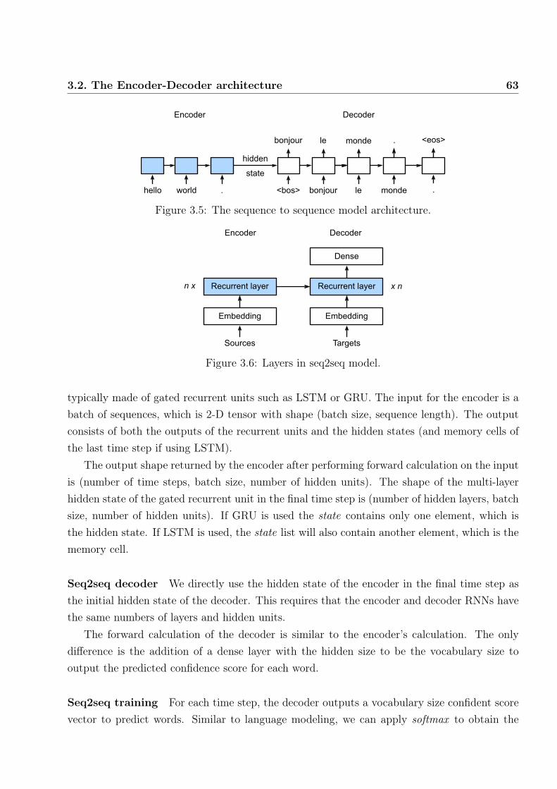
3.2. The Encoder-Decoder architecture 63

Figure 3.5: The sequence to sequence model architecture.

Figure 3.6: Layers in seq2seq model.

typically made of gated recurrent units such as LSTM or GRU. The input for the encoder is abatch of sequences, which is 2-D tensor with shape (batch size, sequence length). The outputconsists of both the outputs of the recurrent units and the hidden states (and memory cells ofthe last time step if using LSTM).

The output shape returned by the encoder after performing forward calculation on the inputis (number of time steps, batch size, number of hidden units). The shape of the multi-layerhidden state of the gated recurrent unit in the final time step is (number of hidden layers, batchsize, number of hidden units). If GRU is used the state contains only one element, which isthe hidden state. If LSTM is used, the state list will also contain another element, which is thememory cell.

Seq2seq decoder We directly use the hidden state of the encoder in the final time step asthe initial hidden state of the decoder. This requires that the encoder and decoder RNNs havethe same numbers of layers and hidden units.

The forward calculation of the decoder is similar to the encoder’s calculation. The onlydifference is the addition of a dense layer with the hidden size to be the vocabulary size tooutput the predicted confidence score for each word.

Seq2seq training For each time step, the decoder outputs a vocabulary size confident scorevector to predict words. Similar to language modeling, we can apply softmax to obtain the

64 Scope

probabilities and then use cross-entropy loss to calculate the loss.But note that we padded the target sentences to make them have the same length. We

would not like to compute the loss on the padding symbols. To solve that, a masked version ofthe loss function is used.

During training, if the target sequence has length n, we feed the first n− 1 tokens into thedecoder as inputs, and the last n − 1 tokens are used as ground truth label. This is calledTeacher Forcing, and is depicted in Fig. 3.5.

Seq2sea prediction To predict a new sequence, the generation process is started by feedingthe same "<bos>" token to the decoder at time step 0, exactly as is done in the training stage.But the input token for a later time step is the predicted token from the previous time step,instead of the ground truth token used during training with the Teacher forcing algorithm.This process is shown in Fig. 3.7.

Figure 3.7: Sequence to sequence model predicting with greedysearch.

Various approaches exist to predict the next token. For example, in Greedy search, thetoken with the highest score at each time step is chosen and used to predict the next token.More details on this will be provided in the next chapter when describing our own model details.

3.2.4 Attention mechanisms

A recent trend in Deep Learning is the use of attention mechanisms, typically added to thedecoder in an encoder-decoder architecture.

Attention is, to some extent, motivated by how we pay visual attention to different regionsof an image or correlate words in one sentence. Human visual attention is well-studied andwhile there exist different models, all of them essentially come down to being able to focus ona certain region of an image with "high resolution" while perceiving the surrounding imagein "low resolution", and then adjusting the focal point over time. Given a small patch of animage, pixels in the rest provide clues about what should be displayed there. For example, ifwe see an eye besides a nose, we expect to see another eye at the opposite side of the nose.

3.2. The Encoder-Decoder architecture 65

Similarly, we can explain the relationship between words in one sentence or a close context.When we see "eating", we expect to encounter a food word very soon.

Attention in Neural Networks has a long history, particularly in image recognition, but onlyrecently have attention mechanisms made their way into recurrent neural networks architecturesthat are typically used in NLP, and increasingly also in computer vision tasks.

3.2.4.1 Attention in Neural Machine Translation

In the original seq2seq model (§3.2.3), the source sequence is encoded into a fixed lengthcontext vector that is then passed to the decoder to generate a target sequence. A critical andapparent disadvantage of the fixed-length context vector design of the initial seq2seq model liesin its incapability of remembering long sentences. Often it has forgotten the first part once itcompletes processing the whole input. The attention mechanism was proposed by Bahdanauet al. (2015) to resolve this weakness.

Besides, often, a token in the target sequence may closely relate to some tokens in the sourcesequence instead of the whole source sequence. For example, when translating "Hello world."to "Bonjour le monde.", "Bonjour" maps to "Hello" and "monde" maps to "world". In theseq2seq model, the decoder may implicitly select the corresponding information from the statepassed by the decoder. The attention mechanism, however, makes this selection explicit.

Below we describe the attention mechanism as originally proposed by Bahdanau et al., andthen we will present a more general model of attention which can be applied to multimodal in-formation tasks such as image captioning, which combines both visual and textual information.

The attention mechanism was born to help memorize long source sentences in neural machinetranslation (NMT). Rather than building a single context vector out of the encoder’s last hiddenstate, the secret sauce invented by attention is to create shortcuts between the context vectorand the entire source input. The weights of these shortcut connections are customizable foreach output element.

While the context vector has access to the entire input sequence, we don’t need to worryabout forgetting. The alignment between the source and target is learned and controlled by thecontext vector. Essentially the context vector consumes three pieces of information: encoderhidden states, decoder hidden states, and alignment between source and target.

More formally: say, we have a source sequence x of length n and try to output a targetsequence y of length m:

x = [x1, x2, . . . , xn]

y = [y1, y2, . . . , ym]

(Variables in bold indicate that they are vectors; same for everything else in this post.)The encoder is a bidirectional RNN (or any other recurrent network setting of your choice)

66 Scope

Figure 3.8: The encoder-decoder model with additive attention mech-anism in (Bahdanau et al., 2015)

with a forward hidden state−→h i and a backward one

←−h i. A simple concatenation of two

represents the encoder state. The motivation is to include both the preceding and followingwords in the annotation of one word.

hi = [−→h >i ;←−h >i ]

>, i = 1, . . . , n

The decoder network has hidden state st = f(st−1, yt−1, ct) for the output word at positiont, t = 1, . . . ,m, where the context vector ct is a sum of hidden states of the input sequence,weighted by alignment scores:

ct =n∑i=1

αt,ihi ; Context vector for output yt

αt,i = align(yt, xi) ; How well two words yt and xi are aligned.

=exp(score(st−1,hi))∑ni′=1 exp(score(st−1,hi′))

; Softmax of some predefined alignment score..

The alignment model assigns a score αt,i to the pair of input at position i and output atposition t, (yt, xi), based on how well they match. The set of {αt,i} are weights defining howmuch of each source hidden state should be considered for each output. In (Bahdanau et al.,2015), the alignment score α is parameterized by a feed-forward network with a single hiddenlayer and this network is jointly trained with other parts of the model. The score function istherefore in the following form, given that tanh is used as the non-linear activation function:

3.2. The Encoder-Decoder architecture 67

score(st,hi) = v>a tanh(Wa[st;hi])

where both va and Wa are weight matrices to be learned in the alignment model.The matrix of alignment scores is a nice byproduct to explicitly show the correlation between

source and target words.

Figure 3.9: Alignment matrix of an French sentence and its Englishtranslation. Source: Fig 3 in (Bahdanau et al., 2015))

3.2.4.2 Different attention mechanisms

With the help of the attention, the dependencies between source and target sequences are notrestricted by the in-between distance anymore. Given the big improvement by attention inmachine translation, it soon got extended into the computer vision field (Xu et al., 2015) andpeople started exploring various other forms of attention mechanisms (Luong et al., 2015; Britzet al., 2017; Vaswani et al., 2017).

Table 3.1 enumerates popular attention mechanisms and their corresponding alignment scorefunctions, where Wa is a trainable weight matrix in the attention layer.

Notes Additive attention is also referred to as additive or concat by other authors. Location-based attention simplifies the softmax alignment to only depend on the target position. Thescaled dot attention is very similar to the dot-product attention except for the scaling factor1/√n; where n is the dimension of the source hidden state.

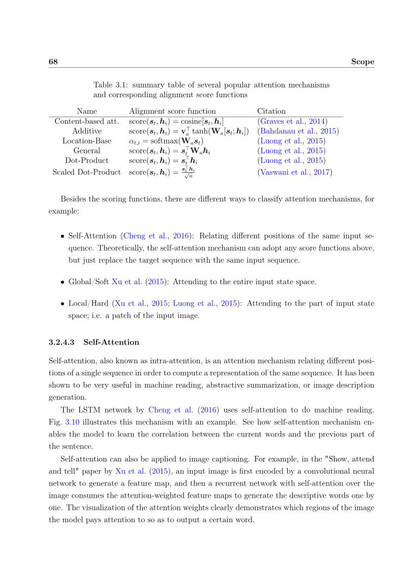
68 Scope

Table 3.1: summary table of several popular attention mechanismsand corresponding alignment score functions

Name Alignment score function CitationContent-based att. score(st,hi) = cosine[st,hi] (Graves et al., 2014)

Additive score(st,hi) = v>a tanh(Wa[st;hi]) (Bahdanau et al., 2015)Location-Base αt,i = softmax(Wast) (Luong et al., 2015)

General score(st,hi) = s>t Wahi (Luong et al., 2015)Dot-Product score(st,hi) = s>t hi (Luong et al., 2015)

Scaled Dot-Product score(st,hi) =s>t hi√n

(Vaswani et al., 2017)

Besides the scoring functions, there are different ways to classify attention mechanisms, forexample:

• Self-Attention (Cheng et al., 2016): Relating different positions of the same input se-quence. Theoretically, the self-attention mechanism can adopt any score functions above,but just replace the target sequence with the same input sequence.

• Global/Soft Xu et al. (2015): Attending to the entire input state space.

• Local/Hard (Xu et al., 2015; Luong et al., 2015): Attending to the part of input statespace; i.e. a patch of the input image.

3.2.4.3 Self-Attention

Self-attention, also known as intra-attention, is an attention mechanism relating different posi-tions of a single sequence in order to compute a representation of the same sequence. It has beenshown to be very useful in machine reading, abstractive summarization, or image descriptiongeneration.

The LSTM network by Cheng et al. (2016) uses self-attention to do machine reading.Fig. 3.10 illustrates this mechanism with an example. See how self-attention mechanism en-ables the model to learn the correlation between the current words and the previous part ofthe sentence.

Self-attention can also be applied to image captioning. For example, in the "Show, attendand tell" paper by Xu et al. (2015), an input image is first encoded by a convolutional neuralnetwork to generate a feature map, and then a recurrent network with self-attention over theimage consumes the attention-weighted feature maps to generate the descriptive words one byone. The visualization of the attention weights clearly demonstrates which regions of the imagethe model pays attention to so as to output a certain word.

3.2. The Encoder-Decoder architecture 69

Figure 3.10: The current word is in red and the size of the blue shadeindicates the activation level. Source: (Cheng et al., 2016).

Figure 3.11: Caption generation example:A woman is throwing afrisbee in a park. Source: (Xu et al., 2015).

70 Scope

3.2.4.4 Soft vs Hard Attention

The soft vs hard attention is another way to categorize how attention is defined. The originalidea was proposed in the "Show, attend and tell" paper (Xu et al., 2015), based on whetherthe attention has access to the entire image or only a patch:

• Soft Attention: the alignment weights are learned and placed "softly" over all patches inthe source image; which corresponds to the additive attention model by Bahdanau et al.(2015).

– Pro: the model is smooth and differentiable.

– Con: expensive when the source input is large.

• Hard Attention: only selects one patch of the image to attend to at a time.

– Pro: less calculation at the inference time.

– Con: the model is non-differentiable and requires more complicated techniques suchas variance reduction or reinforcement learning to train (Luong et al., 2015).

Fig. 3.12 illustrates the soft vs hard effect attention with a visual example from the originalpaper.

Figure 3.12: Comparative of soft (top) vs hard (bottom) attentionduring caption generation. Source: (Xu et al., 2015).

3.2.4.5 Global vs Local Attention

Luong et al. (2015) coined the global vs local attention distinction. The global attention issimilar to the soft attention, while the local one is an interesting blend between hard and soft,an improvement over the hard attention to make it differentiable: the model first predicts asingle aligned position for the current target word and a window centered around the sourceposition is then used to compute a context vector.

Fig. 3.13 compares global and local models of attention in a seq2seq setup.

3.2. The Encoder-Decoder architecture 71

Figure 3.13: Comparative of global (left) vs local (right) attention inthe seq2seq model. Source: (Luong et al., 2015).

The are other models that apply similar ideas and can thus be seen as variations of thesame idea. We will not describe them here, but we enumerate them together:

• The Neural Turing Machine(NTM), by Graves et al. (2014), is a model architecture forcoupling a neural network with external memory storage. The memory mimics the Turingmachine tape and the neural network controls the operation heads to read from or writeto the tape. However, the memory in NTM is finite, and thus it probably looks more likea "Neural von Neumann Machine".

• In problems like sorting or traveling salesman, both input and output are sequential data.Unfortunately, they cannot be easily solved by classic seq2seq or NMT models, given thatthe discrete categories of output elements are not determined in advance, but dependson the variable input size. The Pointer Net (Ptr-Net), was proposed by Vinyals et al.(2015) to address this problem when the output elements correspond to positions in aninput sequence. Rather than using attention to blend hidden units of an encoder into acontext vector (See Fig. 8), the Pointer Net applies attention over the input elements topick one as the output at each decoder step.

• The transformer model introduced in the "Attention is all you need" paper by Vaswaniet al. (2017) is entirely built on the self-attention mechanisms without using sequence-aligned recurrent architecture. It presented a lot of improvements to the soft attention

72 Scope

mechanism, and make it possible to do seq2seq modeling without recurrent network unit,thus reducing the computational costs.

Chapter 4

Model architecture and processes

In this chapter, both the architecture and the training and inference mechanisms of a concretesystem are described. We begin introducing the overall architecture of the system, followed byspecific sections devoted to the different parts of the system: encoder, decoder, and attentionmechanism. Finally, we describe the methods used to train and evaluate the system.

4.1 Overview of the model architecture

As we have discussed in previous section §3.1, we have decided to develop an end-to-end deeplearning solution to the image captioning problem based on an encoder-decoder architecturewith an attention mechanism. This is so far the most common architecture used by state ofthe art systems, as we have seen in our review of the field (Chapter 2.) More specifically, oursystem will consist of the following components:

• Encoder made of a Convolutional Neural Network (CNN)

• Decoder made of a Recurrent Neural Network (RNN)

• Soft Attention mechanism

The general architecture of the system is depicted in Fig. 4.2. To the left of the figure,there is the encoder, which takes an image as input and extracts a feature map. To the right,the decoder has to produce a caption for the input image, using information from its input, itshidden state, as well as the context information received from the attention mechanism. Theattention mechanism lies in between the encoder and the decoder. It is responsible for decidingon which parts of the image (on which features) to focus at each time step while. The attentionmechanism takes the image features and the hidden state of the decoder as inputs and generates

73

74 Model architecture and processes

Figure 4.1: Overview of the model architecture: encoder, decoderand attention mechanism

a context vector, which consists of the features weighted according to some learned weights,which represent the relevance given to each feature at a given moment.

Whilst the encoder generates the features in a single forward step, the decoder has togenerate a caption word by word, one word at a time. To generate the next word it uses theinformation from past states, the current input (the last generated word), and the contextinformation. The process of generating a caption as well as the training procedure will bedescribed later in this chapter.

A more detailed view of the architecture is provided in Fig. 4.2, showing the main layersused in the different components of the system.

• The encoder consists of a CNN module pre-trained on the ImageNet dataset. We takethe output from the last convolutional layer and pass it through a dense, fully connectedlayer to flatten it before passing it to the attention module.

• The decoder consists of an embedding layer that converts input tokens into embeddingvectors, a recurrent layer, which may be made of either GRU or LSTM units, and twostacked fully connected layer that produces the final output. The input is a concatenationof the external input and the context vector from the attention mechanism.

• The attention mechanism actually consists of two fully connected layers, although theyare not showed in the picture. It takes the flattened features from the encoder as input,the hidden states from the decoder, computes attention weights and produces a contextvector as output.

4.2. Encoder 75

Figure 4.2: Detailed architecture showing the layers of each compo-nent

The following sections will describe each component of the network architecture in detail.

4.2 Encoder

The encoder consists of aCNNmodule pretrained on the ImageNet dataset. Several options areavailable for this model. We have included some of the most popular ConvNets, including VGG-16(Simonyan and Zisserman, 2015),Inception-V3(Szegedy et al., 2016), ResNet50(He et al.,2016), and Xception (Chollet, 2017). We also tried to use the NASNet (Zoph et al., 2018) largemodel, but it was impossible due to memory limitations. Finally, we added the InceptionResnetSzegedy et al. (2016) model to the range of options available for the encoder.

As an example, let us assume we are using Inception-V3 for the CNN module. The archi-tecture of this network is shown in Fig. 4.3.

This network receives an image represented by a 3D tensor with shape (229, 229, 3), andgenerates an output consisting of 1001 logits, corresponding to the 1000 classification categoriesin the ImageNet dataset, plus an additional output to denote other things not included inthe labeled categories. However, we are interested in the last convolutional layer, just beforeentering the fully connected block. The output of a convolutional layer is a feature maporganized as a grid of image patches and a number of features per image patch –the depth,or the number of channels. As shown in Fig. 4.3, the output of the Inception-v3 network’slast convolutional layer consists of 8 × 8 × 2048 features, or in general, a 3D tensor of shape

76 Model architecture and processes

Figure 4.3: Overview of the Inception v3 network architecture.Source Google’s Advanced Guide to Inception v3 on Cloud TPU

(fw, fh, fc), where fw and fh are the width and height of the feature map, respectively, and fcis the number of channels. However, instead of using this map as it is, it is squashed into a 2Dtensor, with shape (fw × fh, fc).

Finally, the squashed output of the last convolutional layer is fed into a fully connectedlayer with a ReLu activation function. This layer contains D units, which is a hyperparameterof the model. After forwarding the features map across this layer, we obtain as output a 2Dtensor with shape (L,D), where L is the number of image patches, and D is the number offeatures used to encode each patch (the number of units of the fully connected layer). Notethat from an implementation viewpoint, due to the use of batch processing, we should consideranother dimension in our data, the batch size. However, from a mathematical perspective, andfor the sake of simplicity, we can ignore this additional dimension.

All in all, hereafter, we will use the following notation to represent the output of the encoder.Let us call each set of features for a certain image patch as an annotation vector, denoted byai. Then, the set of feature vectors can be defined as:

a = {a1, ..., aL}, ai ∈ RD

This approach uses the features of the convolutional layer instead of the fully connectedlayer of the encoding CNN. This will allow the decoder to selectively focus on certain parts ofan image by weighting a subset of all the feature vectors.

In our system, the number of features L used to encode images is a configurable hyper-parameter (config .num_features), as is the name of the specific CNN used to extract imagefeatures (config .cnn).

4.3. Decoder 77

4.3 Decoder

The goal of the decoder is to generate a caption for the input image, that is, a sentence thatdescribes what can be seen in the image. We will use y to denote the output of the decoder,which is a sequence of the outputs generated at each time step.

y = {y1, ..., yc}, yi ∈ RK

where K is the size of the vocabulary (number of words), and C is the length of the caption.Each output yi is a vector with size K that represents a probability distributions over thelanguage vocabulary. That is, each element represents the probability of choosing one specificword. There are different ways to choose the final sentence from this sequence of probabilitydistributions, as we will discuss later in this chapter.

The core element of the decoder is a single recurrent layer (named RNN in Fig. 4.2),which consists of a number of recurrent unit with hidden state, either GRU or LSTM unitsindistinctly. Both the type of recurrent unit and the number of units are hyperparameters ofthe model.

In addition to the recurrent layer, the encoder also comprises an embedding layer and twofully connected layers stacked on top of the recurrent layer.

The embedding layer takes an input consisting of a word token, and transforms it intoa dense vector embedding using an embedding matrix E ∈ Rm×K , where m is the dimensionof the embedding vector. During the caption generation process, the input to the embeddinglayer is the last token generated, so we denote the result of the embedding as Eyt−1.

The input to the recurrent layer at a given timestep t will consist of both the result of theembedding layer Eyt−1, a context vector zt coming from the attention mechanism, as well asthe previous hidden state ht−1.

The context vector zt is a dynamic representation of the relevant part of the image inputat time t. Its computation is described in the next section.

The fully connected layers FC1 and FC2 constitute an MLP that is used to generate asequence of words based on the output of the RNN. These two layers make a projection of thehidden state space into the output space. FC1 simple projects the RNN output into a tensorof shape (C, n), where C is the maximum sentence length, and n is the number of RNN units.FC2 takes the output from FC1 and projects it into the final output space, that is, the languagemodel. In particular, this final output is a sequence {y1, ..., yc} of probability distributions ofwords in the vocabulary. That is, each element yi is a 1D tensor with shape (K), made ofvalues in [0,1] representing the probability of a different word from the language vocabulary.There are different methods to convert these probability distributions into a sentence, some

78 Model architecture and processes

which will be described later (§4.6).

4.3.1 Attention

The attention mechanism is responsible for deciding on which parts of the image to focus onat each timestep. In particular, we have designed an attention mechanism inspired by themodel described in Show, Attend and Tell, by Xu et al. (2015), which is in turn based on themechanism proposed by Bahdanau et al. (2015) as an addition to the seq2seq model. Morespecifically, we replicate the soft attention mechanism proposed in the paper. This mechanismweights the features of each part of the image depending on a relevance score that is computedtaking into account the current state of the decoder. This type of attention is called soft,or global, because it attends to the entire input space, unlike hard/local mechanisms, whichattend to a specific location of the input space at any given moment, i.e. a patch of the image.Furthermore, this is a deterministic form of attention, as opposed to stochastic mechanisms,which use probability distributions to select the part of the input to focus at. Finally, thisform attention can also be classified as self-attention, since the decoder attends to the encoderto generate its output, but it is also guided by its own internal state, as we will soon describemore formally. For general information and details on this type of attention, please see §4.3.1.

The output of the attention mechanism is called the context vector zt we have alreadyintroduced. Now let us see how this vector is computed.

We define a mechanism φ that computes zt from the annotation vectors ai, i = 1, ..., L

corresponding to the features extracted at different image locations. For each location i, themechanism generates a positive weight of αi which is interpreted as the relative importance togive to location i in blending the ai’s together. The weight αi of each annotation vector ai iscomputed by an attention model fatt for which we use a multilayer perceptron (not depicted inFig. 4.2), conditioned on the previous hidden state ht−1. To emphasize, note that the hiddenstate varies as the RNN advances in its output sequence: "where" the network looks nextdepends on the sequence of words that have already been generated (represented by the hiddenstate).

eti = fatt(ai, ht−1) (4.1)

The attention weights can be computed from the attention scores eti by scaling to [0, 1] andnormalizing (making weights sum to one).

αti =exp (eti)∑Lk=1 exp (etk)

(4.2)

4.3. Decoder 79

The attention weights represent the alignment between parts of the image and words inthe caption that is being generated, as we will later illustrate with some pictures. Once theattention weights are computed, the context vector zt can be computed by:

zt = φ({ai}, {αi}) (4.3)

where φ is a function that returns a single context vector given the set of annotation vectorsand their corresponding weights. There are different approaches to formulate this functiondepending on the attention model being used. On the one hand, learning a hard –stochastic–attention model requires sampling the attention locations st each timestep. However, for a softattention model, we can take the expectation of the context vector zt directly,

Ep(st|a)[zt] =L∑i=1

αtiai,

and formulate a deterministic attention model by computing a weighted annotation vector

φ({ai}, {αi}) =L∑i=1

αiai, (4.4)

as proposed by Bahdanau et al. (2015). These weighted vectors αi are used as a soft contextthat weights the different parts of the image with variable degrees of relevance, depending onthe state of the decoder, ie. the sentence that has been generated so far. The whole modelis smooth and differentiable under deterministic attention, so learning end-to-end is trivial byusing standard back-propagation.

In particular, to compute the attention weights α we first compute the scores eeti usingthe additive scoring mechanism proposed by (Bahdanau et al., 2015). This mechanism canbe implemented by a multilayer perceptron with a tanh activation function applied over theaddition of the annotation vector (the image features for different image locations), and thehidden state of the decoder’s RNN.

More formally, the attention model fatt is formulated as:

fatt = v>a tanh(W1at +W2ht) (4.5)

where W1, W2, and Va are weights to be learned by backpropagation during the trainingphase.

Finally, note that computing the attention weights αi as defined in Eq. (4.2) is equivalentto applying a softmax function over the attention scores eti. Therefore, equations Eq. (4.1)and Eq. (4.5) can be implemented by a combination of three fully connected layers and two

80 Model architecture and processes

activation functions, as depicted in Fig. 4.4.

Figure 4.4: Detailed architecture of the additive soft attention mech-anism

In our model, the number of units, and thus the dimension of the hidden state, is a config-urable hyperparameter (config .rnn_units). In addition, the type of RNN unit to use is alsospecified as a hyperparameter (config.rnn) with two possible values: ’gru’ or ’lstm’.

4.4 Data pipelines

This section describes the data preparation steps needed to train our model over a benchmarkdataset such as MS COCO. Fitting a model over a big dataset will require processing largeamounts of data, and thus may highly benefit from as much parallelization as possible. Tothat aim, we will organize our data to support parallel pipeline processing by leveraging dataparallelization structures, such as the Dataset class available in Tensorflow.

A general overview of the data pipeline is provided in Fig. 4.5. It all begins with a rawdataset, as the COCO dataset, which consists of a number of images and associated captionsin some dataset-specific format. Then, we perform separate preprocessing tasks for the imagesand for the captions. In order to accelerate training and evaluation tasks, image features arecomputed once and cached to disk. Once image features have been extracted and cached, and

4.4. Data pipelines 81

the captions have been converted into sequences ready to be set into the RNN, images and theirassociated sequences are combined into parallel-efficient data structures supporting bufferingand batching. If the data is being used for training, then it is also randomly shuffled beforegenerating batches.

Figure 4.5: Overview of the data preparation pipeline

The section is organized as follows, first we describe the pre-processing steps required toprepare images for the pipeline, then we describe the steps required to prepare the captions,and finally, we describe the way images and captions are collated together into parallel efficientstructures before being fed to the training or evaluation processes.

4.4.1 Image pre-processing

Images have to be encoded by a CNN to extract the visual features needed by the decoder.In order to be fed into the CNN, images have to be preprocessed first, which includes resizingthem to the shape required by the particular CNN being used, as well as applying tweaks thatare specific of each particular CNN. Some models use images with values ranging from 0 to 1,others from -1 to +1, yet others use the Caffe1 style, that is not normalized but is centered.

1Caffe is an open source deep learning framework, originally developed at University of California, Berkeley.More info can be found at the official website.

82 Model architecture and processes

To support using different ConvNets for the encoder, we have developed a generic methodthat can preprocess images for different models. Table 4.1 summarizes the main characteristicsof some of the most popular ConvNet architectures that are available to the research communityas a pre-trained model, typically trained on the ImageNet dataset.

Table 4.1: Summary of popular ConvNets pretrained on the Ima-geNet dataset

Model Image size Weights size Top-1 acc. Top-5 acc. Params DepthXception 299 x 299 88 MB 0.790 0.945 22,910,480 126VGG16 224 x 224 528 MB 0.715 0.901 138,357,544 23VGG19 224 x 224 549 MB 0.727 0.910 143,667,240 26ResNet50 224 x 224 99 MB 0.759 0.929 25,636,712 168InceptionV3 299 x 299 92 MB 0.788 0.944 23,851,784 159InceptResNetV2 299 x 299 215 MB 0.804 0.953 55,873,736 572MobileNet 224 x 224 17 MB 0.665 0.871 4,253,864 88

Images can be encoded into feature maps beforehand, that is, prior to using them fortraining or inference purposes. That means we only need to generate the image feature mapsonce and save them to disk. To do that aim, in addition to having commands for the trainingand evaluation steps, we have also included a command called prepare which simply generatesand saves to disk image features for a certain CNN.

It is important to remark that for encoding images we are using the features obtained by thelast convolutional layer of the network, excluding the fully connected parts that use to lie at thetop, since these networks are pre-trained for a classification task2. The size of the feature mapsgenerated by the encoding process also differs for different ConvNets. These maps are encodedas grids made of image patches with a certain width W , height H, and depth D. Note thatthe depth is simply the number of features per patch, and is equal to the number of channelsof the last convolution layer. For example, the InceptionV3 model produces feature maps withshape (8× 8× 2048). However, in the end, all the image features will be passed through a fullyconnected layer that will squash them into 2D tensor with shape (L,D), as described in section§4.2.

The specific pre-trained CNN to use in the encoder constitutes a hyperparameter of themodel (config .cnn) which may adopt the following values: ’vgg16’, ’resnet50’, ’inception’,’xception’, and ’nasnet_large’ (although we were unable to use the latest due to lack of mem-ory).

2Typically these models have the weights of the networks that participated in some edition of the ImageNetLarge Scale Visual Recognition Competition (ILSVRC)

4.4. Data pipelines 83

4.4.2 Text pre-processing

Captions are short sentences in natural language. The ultimate goal of the image captioningproblem is to generate captions for new images not included in the training dataset. Therefore,the task of generating a caption can be seen as a task of predicting a sequence of symbols,which implies learning some model of the language. For building such models, we need to turntext into a format that we can optimize over, i.e. we need to map sentences of the languageinto numerical vectors. These vectors provide a numerical representation of the symbols in thelanguage. First of all, we must decide on the level of granularity used to represent the symbolsof the language. One strategy is to treat each word as a unique entity, e.g. (Salton et al., 1975).At the other extreme lies the strategy to predict one character at a time, as suggested e.g. byLing et al. (2015) 3.

Going into details about language models is beyond the scope of this section. Here it sufficesto say that we need a strategy to convert textual captions into a sequence of tokens. A tokenis a data point the model will train and predict. For seq2seq tasks like translation and imagecaptioning the most common approach is to use words as tokens, and that is the approach weadopt here.

4.4.2.1 Tokenization and language modelling

To begin with, we need to split captions into tokens, that is, words. As part of this process, wewill also remove non-alphanumeric characters and punctuation marks.

Then, we need to map tokens into numerical indices. We often call it a vocabulary. Its inputis a list of tokens, called a corpus. Then it counts the frequency of each token in this corpus,and assigns a numerical index to each token according to its frequency, from most frequent tomore rare tokens. The size of the vocabulary is limited, so that rare tokens are removed toreduce the complexity. In order to mark the beginning and end of a sentence, two special tokensare added to the vocabulary: a token named "<start>" (also named "<sos>" or "<bos>")to mark the beginning of sentence, and "<end>" (or "<end>") for the ending of a sentence.Furthermore, another token named "<unk>" is used to represent words that are not includedin the vocabulary. Finally, since we may be representing sentences of different length, we alsoneed a special token named "<pad>" for padding shorter sentences. It is common practice touse 0 as the index of the "<pad>" token so that it is ignored (it has no activation effects).

In our system, the corpus is made of all the captions included in the training dataset.

3Actually, another alternative between both strategies is byte-pair encoding, as described by Sennrich et al.(2016) for the purpose of neural machine translation. It decomposes a text into syllable-like fragments thatoccur frequently. This allows for models that are able to generate words like heteroscedastic or pentagram basedon previously viewed words, e.g. heterogeneous, homoscedastic, diagram, and pentagon

84 Model architecture and processes

We have included configuration options to limit the number of words in the vocabulary. Forexample, for the COCO dataset, the complete corpus consists of almost 30,000 words, but wehave limited the vocabulary size to 10,000 words, which seems to be a reasonable size. Thisvocabulary only has to be built once, since it can be saved and loaded from disk. Needlessto say that the vocabulary must be rebuilt whenever a new corpus is used or the existingcorpus changes. The size of the vocabulary is a configurable hyperparameter of our model(config .vocabulary_size).

One-Hot encoding One-hot encoding vectors provide an easy way to express words as vec-tors in order to process them in a deep network. In a nutshell, we map each word to a differentunit vector: assume that the number of different words in the dictionary is K and each wordhas a one-to-one correspondence with a single value in the index of successive integers from 0 toK − 1. If the index of a word is the integer i, then we create a vector ei of all 0s with a lengthof K and set the element at position i to 1. This vector is the one-hot vector representation ofthe original word.

Word embeddings One-Hot vectors provide a sparse vector representation of words. Wordembedding, however, refers to a technique that uses dense, vectors of real numbers to representwords. Such a vector can be thought of as the feature vector of a word.

Although one-hot word vectors are easy to construct, they are usually not a good choice. Oneof the major reasons is that the one-hot word vectors cannot accurately express the similaritybetween different words, such as the cosine similarity that we commonly use. For the vectorsx,y ∈ Rd, their cosine similarities are the cosines of the angles between them:

x>y

‖x‖‖y‖∈ [−1, 1].

Since the cosine similarity between the one-hot vectors of any two different words is 0, itis difficult to use the one-hot vector to accurately represent the similarity between multipledifferent words.

There are various approaches to learn the word embeddings space, being the skip-gram(Mikolovet al., 2013) and the bag-of-words (BoW) 4 are two of the most popular.

Although there exist open source tools (eg. Word2Vec) and pre-trained language models(Glove) available, for this project we decided to take another approach: learning the embeddingmatrix as an integral part of the complete, end-to-end learning process. This can be a slower

4The BoWmodel is a simplifying representation used in natural language processing and information retrieval(IR). In this model, a text is represented as the bag (multiset) of its words, disregarding grammar and even wordorder but keeping multiplicity. This model dates from Zellig Harris’s 1954 article on Distributional Structure

4.5. Training the model 85

approach but tailors the language model to the task at hand and the specific dataset.

From a practical viewpoint, learning a tailored model can be achieved simply by adding anembedding layer as the first layer of the decoder, as described above (section §4.3). That way,we will not need to embed the words beforehand, as a previous step. Instead, the embeddingmatrix will be learned just like any other layer of the model, and it will suffice with providinga one-hot encoding representation of captions to train the model.

Such an embedding layer has two hyperparameters that are added to our model as config-urable options: the size of the vector space in which words will be embedded (config .embedding_dim),and the size of the vocabulary (config .vocabulary_size)

4.4.3 Dataset generation

We have already described the image preprocessing steps and the text preprocessing that hasto be carried out to prepare our data prior to using it. However, in order to efficiently usethis data as input to the full pipeline of our end-to-end model, we need to organize it intospecial data structures supporting batching, shuffling, prefetching (buffering), and parallelism.Fortunately, Tensorflow a data structure supporting all those features, by the name of Dataset.This structure allows linking together different data sources, as long as the data can be convertedto tensors, which includes all primitive data types. That means we can build an instance ofDataset that collates together the feature maps obtained from a set of images, and the one-hottokenized representations of the captions associated with those images. Therefore, we couldprefetch, shuffle and organize that data in batches.

In our system, we have added the batch size as a hyperparameter that can be customized(config .batch_size).

We have created methods to create two different Dataset instances, one for the trainingportion of the image-caption dataset, and another one its the evaluation portion.

4.5 Training the model

Training is the process of fitting the model to a particular dataset. In many tasks, includingimage captioning, training is supervised, that is, dataset instances are labeled with the solutions.In these cases, the model is fitted to the data by modifying its parameters (eg. the weights ofa neural network) so that a particular loss function is minimized.

In the image captioning problem, the data examples are the images, and the labels are thecaptions, expressed in natural language. Usually, these captions are provided by humans that

86 Model architecture and processes

were asked to describe the images5. In this particular case, the loss function is computed bycomparing word by word the sentence generated by the RNN against the provided caption.However, due to the sequential nature of the output, this is not as simple as computing theloss with non-sequential outputs, like typically happens when solving a classification task. Inparticular, we will use a specific technique named Teacher Forcing, which is often used forlearning sequential models and will be explained below.

4.5.1 Loss function

In order to use supervised training, we need to minimize a loss function. In the image captioningproblem, the error will be related to the generation of the caption: the actual caption constitutesthe ground truth, while the caption generated by the model will be the prediction. However, asequence is not generated in a single step, instead, it is computed word by word, and the losswill be computed word by word. Let us see how the training unfolds sequentially in order tounderstand how to compute a loss function.

On the one hand, the image associated to the example caption is processed by the encoderConvNet and results in a 2D tensor of features, which are then weighted by the attentionmechanism, and conveniently reshaped before being fed into the decoder RNN as. The resultingtensor corresponds to the context explained above (§4.3.1): zt

On the other hand, the caption is converted into a sequence of embedding vectors, once pereach word (Ext). The word embeddings have to be concatenated with the context vectors toproduce the final input to the RNN, but this process does not happen as a single step. Instead,the word embeddings have to be processed one by one, and for each embedding Ext a newcontext vector will be computed by the attention mechanism and concatenated to make theinput at timestep t:

[zt;Ext]

Given that input and the previous hidden state tt−1, the RNN will generate a new outputof yt. The output is a vector of logits with dimension equals to the number of words in thevocabulary, K. That is, each element of the output vector is the probability of a word in thevocabulary. Such output can be interpreted as the prediction of a particular word so that it canbe compared against the ground truth to compute a loss value, where the ground truth refers tothe actual word in the tth position of the caption. This can be seen as a multitask classificationtask, with as many classes as words in the vocabulary. Furthermore, since the ground truth is

5This can be done in large quantities thanks to crowdsourcing marketplaces like the Amazon MechanicalTurk (MTurk).

4.5. Training the model 87

represented using one-hot encoding, then we should use a SparseCategoricalCrossentropy lossfunction to compute the loss between the predicted word and the actual word.

The losses for every word in the sentence will be computed separately and summed togetherto obtain a single loss value. Finally, the accumulated loss shall be divided by the length of thecaption to obtain a loss value that is independent of the length of the caption.

Besides, when computing the loss value, padding tokens should be avoided, which is achievedby using a masked version of the loss function.

4.5.2 Teacher forcing

There are sequence prediction models that use the output from the last time step yt−1 as inputfor the model at the current time step Xt. This type of model is common in language modelsthat output one word at a time and use the output word as input for generating the nextword in the sequence. For example, this type of language model is used in an Encoder-Decoderrecurrent neural network architecture for sequence-to-sequence generation problems such asmachine translation, text summarization, question answering, and image captioning.

Teacher forcing is a strategy for training recurrent neural networks that uses the modeloutput from a prior time step as an input. This method was originally proposed as an alternativetechnique to backpropagation through time for training a recurrent neural network (Williamsand Zipser, 1989).

Teacher forcing works by using the expected output from the training dataset at the currenttime step t as input in the next time step t+1, rather than the output generated by the network,as is the case when the network is predicting a new sequence (as is the case during the validationstage). Let us explain Teacher forcing with a concrete example.

Consider an image of a tennis player with the following caption:

<start> a man standing on a tennis court holding a tennis racquet <end>

Fig. 4.6 depicts the inputs at each time step for the example above. We are not showingthe outputs here because it is not relevant. The loss function will be computed between pairs(input, output), aggregated and divided by the length of the caption.

Teacher forcing is a fast and effective way to train a recurrent neural network that uses theoutput from prior time steps as input to the model. Nevertheless, this approach can also resultin models with poor prediction performance as the RNN’s conditioning context (the sequence ofpreviously generated samples) diverge from sequences seen during training(Lamb et al., 2016).This is common in most applications of this type of model as the outputs are probabilistic innature. This type of application of the model is often called open loop.

88 Model architecture and processes

Figure 4.6: Teacher forcing for image captioning training. The ex-pected word is used as input of the network at each timestep

4.6 Inference and validation

After the model is trained, it can be used to generate new sequences. To do that, we shouldsimply feed a "<start>" token to the RNN start the process, and the generated word in theoutput sequence will then be used as input on the subsequent time step, along with the contextvector coming from the attention mechanism. This process is depicted in Fig. 4.7

The generation process will continue until the "<end>" token is reached, or a maximumsequence length is reached.

Figure 4.7: Word-by-word caption generation

Various approaches exist to predict the next token. For example, when using Greedy search,the token with the highest score at each time step is chosen and used to predict the next token.However, there are more sophisticated approaches, introduce below.

For ease of discussion, we assume that the output of the decoder is a sequence of text.Let the size of output text dictionary Y (contains special symbol "<end>") be |Y|, and themaximum length of the output sequence be T ′. There are a total O(|Y|T

′) types of possible

output sequences. All the subsequences after the special symbol "<end>" in these outputsequences will be discarded.

4.6. Inference and validation 89

4.6.1 Greedy Search

First, we will take a look at a simple solution: Greedy search. For any time step t′ of the outputsequence, we are going to search for the word with the highest conditional probability from |Y|numbers of words, with

yt′ = argmaxy∈Y

P(y | y1, . . . , yt′−1, c)

as the output. Once the "<end>" symbol is detected, or the output sequence has reachedits maximum length T ′, the output is completed.

As we mentioned in our discussion of the decoder, the conditional probability of generatingan output sequence based on the input sequence is

∏T ′

t′=1 P(yt′ | y1, . . . , yt′−1, c). We will takethe output sequence with the highest conditional probability as the optimal sequence. Themain problem with Greedy search is that there is no guarantee that the optimal sequence willbe obtained.

Take a look at the example in Fig. 4.8. We assume that there are four words "A", "B", "C",and "<end>" in the output dictionary. The four numbers under each time step represent theconditional probabilities of generating "A", "B", "C", and "<end>" at that time step. At eachtime step, greedy search selects the word with the highest conditional probability. Therefore,the output sequence "A", "B", "C", "<end>" will be generated in Fig. 4.8. The conditionalprobability of this output sequence is 0.5× 0.4× 0.4× 0.6 = 0.048.

Figure 4.8: The four numbers under each time step represent theconditional probabilities of generating "A", "B", "C", and "<end>"at that time step. At each time step, greedy search selects the wordwith the highest conditional probability.

Now, we will look at another example shown in Fig. 4.9. Unlike in Fig. 4.8, Fig. 4.9 selectsthe word "C" for it has the second highest conditional probability at time step 2. Since theoutput subsequences of time steps 1 and 2, on which time step 3 is based, are changed from"A" and "B" in Fig. 4.8 to "A" and "C" in Fig. 4.9, the conditional probability of each wordgenerated at time step 3 has also changed in Fig. 4.9. We choose the word "B", which has thehighest conditional probability. Now, the output subsequences of time step 4 based on the first

90 Model architecture and processes

three time steps are "A", "C", and "B", which are different from "A", "B", and "C" in Fig. 4.8.Therefore, the conditional probability of generating each word in time step 4 in Fig. 4.9 is alsodifferent from that in Fig. 4.8. We find that the conditional probability of the output sequence"A", "C", "B", "<end>" at the current time step is 0.5×0.3×0.6×0.6 = 0.054, which is higherthan the conditional probability of the output sequence obtained by greedy search. Therefore,the output sequence "A", "B", "C", "<end>" obtained by the greedy search is not an optimalsequence.

Figure 4.9: The four numbers under each time step represent theconditional probabilities of generating "A", "B", "C", and "<end>"at that time step. At time step 2, the word "C", which has the secondhighest conditional probability, is selected.

4.6.2 Exhaustive Search

If the goal is to obtain the optimal sequence, we may consider using Exhaustive search: anexhaustive examination of all possible output sequences, which outputs the sequence with thehighest conditional probability.

Although we can use an exhaustive search to obtain the optimal sequence, its computationaloverhead O(|Y|T

′) is likely to be excessively high. For example, when |Y| = 10000 and T ′ = 10,

we will need to evaluate 1000010 = 1040 sequences. This is next to impossible to complete.The computational overhead of greedy search is O(|Y|T ′), which is usually significantly lessthan the computational overhead of an exhaustive search. For example, when |Y| = 10000 andT ′ = 10, we only need to evaluate 10000× 10 = 1× 105 sequences.

4.6.3 Beam search

Beam search is an improved algorithm based on Greedy search. It has a hyper-parameternamed beam size. We set it to k. At time step 1, we select k words with the highest conditionalprobability to be the first words of the k candidate output sequences. For each subsequent timestep, we are going to select the k output sequences with the highest conditional probability fromthe total of k |Y| possible output sequences based on the k candidate output sequences from the

4.6. Inference and validation 91

previous time step. These will be the candidate output sequence for that time step. Finally, wewill filter out the sequences containing the special symbol "<end>" from the candidate outputsequences of each time step and discard all the subsequences after it to obtain a set of finalcandidate output sequences.

Figure 4.10: The beam search process. The beam size is 2 and themaximum length of the output sequence is 3. The candidate outputsequences are A, C, AB, CE, ABD, and CED.

Fig. 4.10 demonstrates the process of beam search with an example. Suppose that thevocabulary of the output sequence only contains five elements: Y = {A,B,C,D,E} where oneof them is a special symbol “<end>”. Set beam size to 2, the maximum length of the outputsequence to 3. At time step 1 of the output sequence, suppose the words with the highestconditional probability P(y1 | c) are A and C. At time step 2, we compute P(A, y2 | c) = P(A |c)P(y2 | A, c) and P(C, y2 | c) = P(C | c)P(y2 | C, c) for all y2 ∈ Y , and pick the largest twoamong these 10 values: say P(A,B | c) and P(C,E | c). Then at time step 3, we computeP(A,B, y3 | c) = P(A,B | c)P(y3 | A,B, c) and P(C,E, y3 | c) = P(C,E | c)P(y3 | C,E, c)for all y3 ∈ Y , and pick the largest two among these 10 values: say P(A,B,D | c) andP(C,E,D | c). As a result, we obtain 6 candidates output sequences: (1) A; (2)C; (3) A, B;(4)C, E; (5)A, B, D; and (6)C, E, D. In the end, we will get the set of final candidate outputsequences based on these 6 sequences.

In the set of final candidate output sequences, we will take the sequence with the highestscore as the output sequence from those below:

92 Model architecture and processes

1

LαlogP(y1, . . . , yL) =

1

Lα

L∑t′=1

logP(yt′ | y1, . . . , yt′−1, c),

Here, L is the length of the final candidate sequence and the selection for α is generally0.75. The Lα on the denominator is a penalty on the logarithmic addition scores for the longersequences above. The computational overhead O(k |Y|T ′) of the beam search can be obtainedthrough analysis. The result is a computational overhead between those of greedy search andexhaustive search. In addition, Greedy search can be treated as a beam search with a beamsize of 1. Beam search strikes a balance between computational overhead and solution qualityusing a flexible beam size of k.

Note: In the developed system, we have implemented both greedy search and beam search,however, results with Beam search hasn’t been satisfactory.

4.7 Implementation

The software developed for this Master Thesis Project is available as an open source projectunder a Creative Commons license (CC Attribution-ShareAlike 4.0). The code repository canbe found here: https://github.com/magomar/image_captioning_with_attention

Chapter 5

Experiments

5.1 Dataset

We were considering four datasets to conduct our experiments. We also considered usingtwo or more datasets, but in the end, we decided to perform all our experiments using thecurrent benchmark dataset, the one that is used by researchers to compare their models andpublish their results: The COCO dataset, released by Microsoft in 2014 Lin et al. (2014). Atthe moment of writing this report, this is without a doubt the preferred benchmark datasetfor the image captioning problem. In addition, there is an online server that automates theevaluation and comparison of submitted results. This server is running 24/7, and results arepublicly available, so it is actually an open competition, known as the Microsoft COCO ImageCaptioning Challenge.

Figure 5.1: Image caption examples. Source: COCO Image Caption-ing Task

In the end, we only used this dataset because the other common options are clearly outdated,such as the Flickr8K and Flickr30K. Although the latter was deemed as an interesting option

93

94 Experiments

for faster experiments in the first stages of the project, we finally upgraded the hardware witha very powerful GPU that made it feasible to use the COCO dataset as the only experimentaldataset, and still conduct a considerable number of experiments.

As a matter of fact, there is still a larger dataset supporting image captioning, the Concep-tual Captions dataset, by Google (Sharma et al., 2018), which also offers an online evaluationserver and a public leaderboard. However, it was released just a few months ago, and it is sohuge, that it will probably take sometime before it is widely adopted by researchers1.

For our project, we are using the images and the associated captions included in this dataset,which are divided into two separate sets: one for training, and another one for validationpurposes.

5.1.0.1 Training dataset

This dataset includes a total of 82.783 unique images which are supposed to have 5 captionseach, which would amount to 413.915 captions. However, there are actually 414.113, probablybecause some image has more than 5 captions.

The length (number of words) of the captions is highly variable, with a maximum length of51. The full corpus of text in the training captions dataset is 31.437.

After some initial analysis on the set of captions, we realized that a vast majority of cap-tions are much shorter than the maximum length, therefore, for the sake of speeding up theprocessing of the recurrent layer, we decided to restrict the dataset to those captions havinga maximum length of 15, which implied removing 13.370 images and 66.885 captions from thetraining dataset. This filter was applied before tokenizing the captions, thus in practice, whenincluding the "<start>" and "<end>" tokens the maximum length of a sequence would be 17.Note the maximum length of the captions is actually a configurable parameter of the model(config .max_caption_length)

All in all, after filtering the dataset on a maximum caption length basis, we end up with adataset containing 347.228 instances, each one consisting of a single caption and its associatedimage.

Concerning the vocabulary, the resulting corpus contains 24.775 words, which is still a hugenumber, considering that many words only appear once. Finally, we decided to set the vocabu-lary size to 10,000. The words excluded from the vocabulary were assigned the "<unk>" token.The size of the vocabulary is another hyperparameter of the model (config .vocabulary_size).

1When I started this project there were no results yet but the ones published by Google. A month laterthere are already four additional results from two different teams

5.2. Experiments 95

5.1.0.2 Validation dataset

The full validation dataset contains 40504 images and 5 captions per image. After applying thesame filtering schema based on the maximum length of the captions, the dataset was reducedto 34043 images

Note that for the training process, each instance is made up of one single caption andits associated image, whilst for the evaluation process, each instance is an image and all itsassociated captions.

5.2 Experiments

5.2.1 Experimental setup

All the experiments reported in this chapter were performed on the MSCOCO dataset, withthe additional constraints described above, which resulted in two separated datasets, one forthe training, and another one for validations. Summing up:

• Training: 347,228 examples, each one consisting of an image-caption pair

• Validation: 34043 examples, each one consisting of an image, and all their captions (5captions per image)

Caption length is limited to 15 significant tokens, plus the "<start>" and "<end>" token.Hardware setup:

• CPU: Intel Core i7-4790K (4 cores, 8 threads clocked @ 4 GHz)

• RAM: 16GB DIMM DDR3 2400 (clocked @ 1333 MHz)

• Data Storage: SSD Samsung 850 Evo 250GB

• GPU-0: NVIDIA GTX 1070, 6GB RAM

• GPU-1: NVIDIA RTX 2080 Ti, 11GB RAM

We will not give detailed timing results, because the computer was used interactively toperform other tasks while it was training, but we will make some comments on time aspectswhenever there is something relevant to mention. For the moment, it suffices to say that inmost cases, a full training epoch took between 40 and 50 minutes to complete.

96 Experiments

5.2.2 Overview of the experiments

For the experiments we trained the same basic models but changing some hyperparameters:

• Type of ConvNet: ’VGG16’, ’incept’, ’Xception, ’ResNet50’, ,’InceptionResNet_v2’

• Type of recurrent units: ’GRU’ or ’LSTM’

• Number of recurrent units: 256, 512

• Embedding dimension: 256, 512

• Number of image features: 256, 512, 1024

• Batch size: 64, 128

• Dropout percentage: 0, 0.3, 0.5

Unfortunately, due to the long time required to train each model, we were unable to sys-tematically try all the combinations of the chosen hyperparameters.

We trained all the models for 30 epochs. In one case we trained the model for 90 epochs,but the results clearly indicated that the model was overfitting. Therefore, we conducted someadditional experiments to analyze the problem, and finally, we came up adding some Dropoutlayers as a form of regularization. All these experiments will be analyzed below.

To have a sense of the kind of experiments performed, Table 5.1 provides a summary of themain block of experiments performed. In these experiments, we did not apply regularizationand the training lasted 30 epochs. CNN and RNN are the types of ConvNet and RecurrentNetrespectively, Emb refers to the size of the embedding vectors, Feat is the number of visualfeatures used as input, Batch refers to the batch size, Optimi to the optimizer function, B1-B4are Ble scores, MET refers to Meteor, R refers to ROUGE, and C to CIDEr. Results in thistable are sorted by CIDEr score.

5.2.2.1 Effect of hyperparameters on performance

In order to study the effect of the different hyperparameters of the model on the performance,we have grouped and average the results for different combinations of parameters. Fig. 5.2a andFig. 5.2b compares the performance depending on different types of network, for the encoderand decoder respectively. The other figures compare the performance of the model dependingon some numerical hyperparameters, such as the batch size, the number of hidden units, theembedding size, or the number of image features that are generated by the encoder.

5.2. Experiments 97

Table 5.1: Evaluation results. Model trained for 30 epochs. Noregularization applied.

CNN RNN Emb Hid Feat Batch Optim B1 B2 B3 B4 MET ROU CIDincep-res lstm 512 512 512 64 Adam 0.485 0.320 0.203 0.127 0.162 0.357 0.413inception lstm 256 512 256 128 Adam 0.510 0.337 0.213 0.131 0.164 0.364 0.410inception lstm 256 512 256 64 Adam 0.521 0.342 0.215 0.132 0.166 0.367 0.406inception lstm 512 512 256 64 Adam 0.532 0.346 0.215 0.132 0.170 0.365 0.394inception gru 512 512 512 64 Adam 0.509 0.330 0.205 0.125 0.162 0.357 0.390inception gru 256 512 256 64 Adam 0.503 0.329 0.206 0.127 0.160 0.357 0.388inception gru 256 512 256 64 Nadam 0.515 0.336 0.209 0.127 0.163 0.360 0.380inception lstm 256 512 1024 128 Adam 0.509 0.327 0.201 0.121 0.162 0.355 0.370xception gru 256 512 256 64 Adam 0.507 0.326 0.199 0.120 0.160 0.352 0.365inception gru 512 1024 512 128 Adam 0.490 0.314 0.192 0.116 0.155 0.347 0.355resnet lstm 256 512 512 128 Adam 0.463 0.302 0.188 0.115 0.152 0.342 0.351

(a) Scores by type of ConvNet (b) Scores by type of RNN unit

(a) Scores by batch size (b) Scores by number of recurrent units

98 Experiments

(a) Scores by embedding dimension (b) Scores by number of image features

By looking at the former graphs, and at the correlation matrix in Fig. 5.5, we can see thefollowing relations between the hyperparameters and the scores measured over the validationdataset.

• In general, there is a high degree of correlation between the different metrics except forCIDEr, that shows the least correlation with the other metrics.

• In all the numerical hyperparameters we observe a moderately negative correlation withthe scoring metrics. That is, the higher the value of the hyperparameter the worse scoringobtained. Why is that? In general, higher values in these parameters (ie. more units,larger batches) make the model more complex, which in turn increases the bias. Therefore,by having set up a fixed number of training epochs, this observation is consistent withoverfitting. That is, since the model is overfitting, increasing the complexity of the modelcan only aggravate the problem.

5.2.2.2 Training and overfitting

Overfitting occurs when a model performs very well with the training dataset, but not so wellwith other data, that is, the model does not generalize well. Overfitting can be discovered bycomparing the performance over the training dataset and the validation dataset. Usually, thesame loss function is used in both cases and it is pretty easy to find out if a model is overfitting.In the image captioning problem and other problems in NLP, this is not so easy because theprediction stage is different from the training stage (recall the teacher forcing technique usedto generate captions in our model). Furthermore, language tasks use sophisticated metrics toestimate the quality of the model. In these cases, overfitting can be discovered by studying thedynamics of the system. Typically, we will see a stall o even a deterioration in the performance

5.2. Experiments 99

Figure 5.5: Correlation matrix for the numeric hyperparameters andthe performance metrics

although the training loss continues decreasing. Ideally, we would interleave training and val-idation to detect this kind of problems as soon as possible. By doing this we can stop thetraining to avoid wasting time and keep a copy of the model when it was performing the better.This technique is called early stopping, and can be seen as a specific form of regularization.

We did not include an automatic validation mechanism interleaved with the training process;however, we did perform various analysis of the dynamics of the model by keeping checkpoints,that is, by saving the model at different moments along the training process, and evaluatingmultiple models afterward. An example of such an analysis can be seen in Fig. 5.6. Clearly,there is a point, around the 6th epoch, when the metric scores worsen, while the training lossis still decreasing. This behavior is a clear sign of overfitting.

There are various approaches to avoid or diminish overfitting. Two of the most populartechniques applied in deep learning are dropout and batch normalization.

5.2.2.3 Dropout regularization

In the last stage of the project we did manage to include some degree of regularization byintroducing dropout layers just before dense layers in the different components of the model:the encoder, the decoder, and also the attention mechanism. We did not have to time for asystematic analysis, but preliminary results showed that this solution delayed the overfittingfor several epochs, although in the end there was overfitting. We expect to delve deeper intothis technique in the future to improve our results. Also, it would be interesting to try other

100 Experiments

Figure 5.6: Evolution of loss and performance as training progresses

mechanisms such as batch normalization.As illustration of the effect obtained by dropout, compare Table 5.2 and Table 5.3. These

tables show results of the same model for 10 epochs, showing the metric scores of the validationevery 2 epochs. However, the first one does not include dropout, and the second one includesa dropout of 0.3 (probability of letting a unit out during training)

Table 5.2: Some results of training and validation without normal-ization

Epochs Loss Bleu1 Bleu2 Bleu3 Bleu4 METEOR ROUGE CIDEr2 1.56763 0.448 0.302 0.191 0.119 0.152 0.354 0.3624 1.439718 0.492 0.339 0.223 0.143 0.168 0.378 0.456 1.357404 0.501 0.345 0.229 0.149 0.171 0.381 0.4728 1.296668 0.497 0.34 0.223 0.145 0.169 0.377 0.46610 1.261107 0.498 0.338 0.22 0.141 0.168 0.376 0.461

5.2.3 Demonstrative examples

We conclude this section by showing some examples of the captions generated by our modelusing some examples from the validation dataset.

5.2. Experiments 101

Table 5.3: Some results of training and validation with dropout =0.3

Epochs Loss Bleu1 Bleu2 Bleu3 Bleu4 METEOR ROUGE CIDEr2 1.562302 0.466 0.324 0.214 0.137 0.161 0.369 0.4344 1.431397 0.496 0.346 0.231 0.15 0.171 0.381 0.4786 1.350335 0.511 0.357 0.239 0.154 0.175 0.387 0.4958 1.285521 0.522 0.363 0.24 0.154 0.177 0.387 0.49410 1.237422 0.517 0.356 0.235 0.15 0.175 0.383 0.484

As you can see, in general the system has been able to detect some of the main elements ofthe picture, although not all of them. Many times some elements of the image are not includedin the caption, or there are errors. Sometimes, there is a clear error, like not detecting thetruck in Fig. 5.11, or error in the quantity of an important element of the image, such as thenumber of people in Fig. 5.9.

Concerning the structure of the generated captions, the majority of them are grammaticallycorrect, and most of the problems identified are rather semantic, like the double mention to"chocolate" in Fig. 5.14.

102 Experiments

Figure 5.7: Ground Truth: A man standing on a tennis court holdinga tennis racquet.

Figure 5.8: Predicted: a tennis player is getting ready to hit a tennisball.

5.2. Experiments 103

Figure 5.9: Ground Truth: Two males and a female walking in thesnow carrying a ski sled and snowboard.

Figure 5.10: Predicted: a person riding skis ride down a snowy hills.

104 Experiments

Figure 5.11: Ground Truth: A man sitting on the back of a red truck.

Figure 5.12: Predicted: a group of people are posing for a red coveredlawn.

5.2. Experiments 105

Figure 5.13: Ground Truth:a man is holding a piece of food withchocolate in it.

Figure 5.14: Predicted: A person holding a piece of chocolate cakewith a chocolate cake.

106 Experiments

Chapter 6

Conclusions

This chapter presents a critical self-opinion of the project and collects a number of potentialimprovements and future work.

6.1 What I learned

This project has supposed a huge advancement in my understanding of deep learning, especiallyin the fields of Natural Language Processing (NLP) and Computer Vision (CV).

To begin with, I had to review a lot of literature on the topics of the project. Furthermore,being a project that combines NLP and CV, it covered a vast number of concepts, models andtechnologies. The initial stages of the project, where I was supposed to collect informationon the project and review the state of the art, easily exceeded the expected effort by twiceor tribble at least. One paper led to another paper, one model was soon discovered to havebeen surpassed by other models the following year, and so on. In the end, I expend more thana month actively researching the subjects, plus some extra days collecting and summarizingbenchmark results from several, some times contradictory sources.

Secondly, I combined my research-oriented efforts with an intense self-learning programwhich basically took me through the 5 courses of the Deep Learning specialization programby deeplearning.ai and professor Andrew Ng. at Coursera. Those courses gave me a wideand solid knowledge of deep learning, NLP and CV, combining both theory knowledge withhands-on experience, although the pace was probably too fast as to get a deep understandingof all the content: techniques to develop and improve deep networks, ConvNets, sequence, andrecurrent networks, etc. There were many practical exercises, which were done using Pythonand Tensorflow on Jupyter Notebook. The case studies ranged from healthcare and autonomousdriving to music generation, and natural language processing. All this knowledge was probablytoo much to digest in barely two months, but I still got a grasp of many of the concepts and

107

108 Conclusions

techniques described in the courses, which was of great help to understand the research papersand model implementations I had to review as part of the project.

Third, I had to put into practice many of the concepts and techniques learned. Theseincluded fully connected layers, which I was already familiar with, but also ConvNets, RNNs,language modeling, seq2seq models, attention mechanisms, beam search, and so many other,most of which were new to me. In the beginning, started implementing quick prototypes asa proof of concept, to make sure my hardware had enough computational power to handle abig dataset, as was my intention. To that avail, I started prototyping by means of the JupyterNotebook platform. Preliminary results made me buy a more powerful GPU, as describedin §3.1. Soon, I jumped from the prototyping environment into a fully-fledged developmentenvironment, which included the following tools and technologies:

• Linux operating system, with CUDA drivers for GPU support Visual Studio Code editor

• Git control version and a remote GitLab repository

• Conda and Pip for package management

• Tensorflow 2.0.0-alpha with GPU support, and Keras API.

6.1.1 What I would have changed

The development of a working system was an intense and very exciting experience too, but theentire development effort was highly conditioned from the very beginning by an excruciatinglack of time. As a matter of fact, the analysis of the problem and the review of the literatureconsumed too much of my time, and thereafter I felt severely pushed by this lack of time, whichmade me commit several mistakes.

• First and probably the most severe mistake was developing and debugging the systemusing a big dataset. Once I realize I needed a smaller dataset for the initial developmentstage, I limited the number of examples actually used from the dataset, but as soon asI obtained an apparently working system I moved into the full dataset. By doing this, Ihad to expend a lot of time waiting for results rather than tweaking and improving themodel.

• A second mistake that aggravated the former was the lack of a proper evaluation mech-anism, which was delayed until the latest stages of the development process, when Iincluded a tool to compute the usual metrics (Bleu, Meteor, etc.). Even worse, I didn’ttake the effort to interleave validation and training, that is, to check the generalization

6.2. Future work 109

ability of the network as the training progressed. Too late I realized that the model wastremendously overfitting, as shown in the experimental section (Chapter 5.

The combination of the two mistakes above made me waste a lot of time and computing re-sources overfitting the model far beyond the sweet spot. I couldn’t imagine how soon overfittingstarted, but it was too late. However, this is a lesson I will never forget.

6.1.2 What I did not expect

In general, the different experiments with the model performed considerably worse than ex-pected considering the results achieved by the model it was inspired by, the one described inthe "Show, attend and tell" paper by Xu et al. (2015). However, but I have yet to find outwhether this is due to implementation details, the lack of proper fine-tuning of the parameters,or a combination of the former.

The most frustrating result was due to the bad performance obtained by the beam searchalgorithm. It took several hours to develop a working beamsearch algorithm. However, it wasincredibly slow, and yet it obtained worse results than using greedy search, which was utterlyunexpected. I should have to investigate this in the future since I am really disappointed.

After conducting a number of experiments with attention and still not getting as good resultsas expected, I decided to compare the model with attention against the same model withoutattention. For that purpose, I modified the existing model and conducted various experiments,but something was probably wrong because I couldn’t obtain any reasonable results to compareagainst, but I did not have more time to debug it.

6.2 Future work

The limited time prevented me from adopting a more systematic and thorough approach tothe development of a solution. In this final section I will enumerate some of the many thingsthat could be done to complete, improve or extend the developed system, as well as alternativeapproaches to the image captioning problems, which include published work as well as someideas that come to my mind based on what I have learned during this project.

First of all, some validation should be included as an integral part of the training pro-cess to monitor it and detect overfitting, perhaps combined with early stopping as a form ofregularization.

Second, given the results obtained, overfitting arises as one of the major problems with themodel developed. Unfortunately, I realized very late the need for regularization mechanisms,

110 Conclusions

such as batch normalization and dropout. This would be the most important improvements toundertake in the future, combined with the use of validation during the training procedure.

Third, it would be convenient to conduct more experiments, and in a more principled way,so as to have a proper distribution of values for the most important hyperparameters. It wouldbe also very helpful to perform most of these experiments on a smaller dataset, such as theFlickr8K or the Flickr30K datasets, to get a more comprehensive understanding on the effectsof the various hyperparameters and how to tune them before moving into larger datasets.

Fourth, it would be nice to have a baseline to compare against, such as the same basic modelwithout the attention mechanism. Actually, I tried to do this but something went wrong andI did not have time enough to debug it.

Finally, in addition to monitoring validation while training, it would also be very interestingto include some form of visualization, probably by means of the Tensorboard visualization tool.This is something I did not have the opportunity to explore, but I would definitely add this assomething to address in the future.

Besides the proposed improvements, there are a number of things that could be done in thefuture to extend the work done for this project.

• To begin with, it would be nice to develop alternative models of attention to compare with,such as the global attention mechanism proposed by Luong et al. (2015) or a hierarchicalattention mechanism as the one proposed by Khademi and Schulte (2018).

• I’m really curious about the possibility of adding reinforcement learning to improve thecaptioning process, in the likes of the model proposed by Rennie et al. (2017).

• Finally, aside from other forms of attention and alternative methods to generate captions,it would be nice to build an online application for demonstrative purposes. Since ourmodel was developed in Tensorflow, it would be easy to load the model into a Web Appby means of the Tensorflow.js library.

6.3 Concluding remarks

All in all, retrospectively, I am very happy with having chosen this problem for my MasterThesis. It is a very challenging problem, and it was very exciting as a research problem. Asa matter of fact, I ended up dedicating far more time than planned surveying the state of theart, but I did not regret this at all; it was quite inspiring to see so many advances in such abrief period of time.

6.3. Concluding remarks 111

However, I felt like I would have needed far more time to develop a more satisfactory system.In the end, the results were not up to my expectations, and I am looking forward to improvingand extending it in my free time in the near future.

The code for the project

112 Conclusions

Bibliography

Anderson, P., Fernando, B., Johnson, M., and Gould, S. (2016). SPICE: Semantic PropositionalImage Caption Evaluation. In 4th European Conference on Computer Vision (ECCV’16),pages 382–398. Springer.

Anderson, P., Gould, S., and Johnson, M. (2018a). Partially-Supervised Image Captioning. In32nd Conference on Neural Information Processing Systems (NeurIPS 2018), Montreal.

Anderson, P., He, X., Buehler, C., Teney, D., Johnson, M., Gould, S., and Zhang, L. (2018b).Bottom-Up and Top-Down Attention for Image Captioning and Visual Question Answering.In 2018 IEEE/CVF Conference on Computer Vision and Pattern Recognition, pages 6077–6086, Salt Lake City, USA. IEEE.

Aneja, J., Deshpande, A., and Schwing, A. G. (2018). Convolutional Image Captioning. In2018 IEEE/CVF Conference on Computer Vision and Pattern Recognition (CVPR), pages5561–5570, Salt Lake City, USA. IEEE.

Antol, S., Agrawal, A., Lu, J., Mitchell, M., Batra, D., Zitnick, C. L., and Parikh, D. (2015).VQA: Visual Question Answering. In 2015 IEEE International Conference on ComputerVision (ICCV), pages 2425–2433. IEEE.

Bach, F. and Jordan, M. (2003). Kernel independent component analysis. In 2003 IEEE In-ternational Conference on Acoustics, Speech, and Signal Processing (ICASSP’03), volume 4,pages IV–876–9, Hong Kong, China. IEEE.

Badrinarayanan, V., Kendall, A., and Cipolla, R. (2017). SegNet: A Deep ConvolutionalEncoder-Decoder Architecture for Image Segmentation. IEEE Transactions on Pattern Anal-ysis and Machine Intelligence, 39(12):2481–2495.

Bahdanau, D., Cho, K., and Bengio, Y. (2015). Neural Machine Translation by Jointly Learn-ing to Align and Translate. In 2015 International Conference on Learning Representations(ICLR), San Diego, USA.

113

114 BIBLIOGRAPHY

Bai, S. and An, S. (2018). A survey on automatic image caption generation. Neurocomputing,311:291–304.

Banerjee, S. and Lavie, A. (2005). METEOR: An Automatic Metric for MT Evaluation withImproved Correlation with Human Judgments. In Proceedings of the ACL Workshop onIntrinsic and Extrinsic Evaluation Measures for Machine Translation and/or Summarization,pages 65–72, Ann Arbor, USA. Association for Computational Linguistics.

Barto, A. G., Sutton, R. S., and Anderson, C. W. (1983). Neuronlike adaptive elements thatcan solve difficult learning control problems. IEEE Transactions on Systems, Man, andCybernetics, SMC-13(5):834–846.

Berg, T. L., Berg, A. C., and Shih, J. (2010). Automatic Attribute Discovery and Character-ization from Noisy Web Data. In Proceedings of the 9th European Conference on ComputerVision (ECCV).

Berger, A. L., Pietra, S. A. D., and Pietra, V. J. D. (1996). A Maximum Entropy Approach toNatural Language Processing. Computational Linguistics, 22(1):39–71.

Bernardi, R., Çakici, R., Elliott, D., Erdem, A., Erdem, E., Ikizler-Cinbis, N., Keller, F.,Muscat, A., and Plank, B. (2017). Automatic description generation from images: A surveyof models, datasets, and evaluation measures. IJCAI International Joint Conference onArtificial Intelligence, 55:4970–4974.

Blei, D. M., Ng, A. Y., and Jordan, M. I. (2003). Latent Dirichlet Allocation. Journal ofMachine Learning Research, 3:993–1022.

Britz, D., Goldie, A., Luong, M.-T., and Le, Q. (2017). Massive Exploration of Neural MachineTranslation Architectures. In Proceedings of the 2017 Conference on Empirical Methodsin Natural Language Processing, pages 1442–1451, Stroudsburg, PA, USA. Association forComputational Linguistics.

Buschman, T. J. and Miller, E. K. (2007). Top-Down Versus Bottom-Up Control of Attentionin the Prefrontal and Posterior Parietal Cortices. Science, 315(5820):1860–1862.

Bychkovsky, V., Paris, S., Chan, E., and Durand, F. (2011). Learning photographic global tonaladjustment with a database of input / output image pairs. In CVPR 2011, pages 97–104.IEEE.

Callison-Burch, C., Osborne, M., and Koehn, P. (2006). Re-evaluating the Role of BLEU inMachine Translation Research. In Proceedings of 11th Conference of the European Chapterof the Association for Computational Linguistics, Trento, Italy.

BIBLIOGRAPHY 115

Chen, L., Zhang, H., Xiao, J., Nie, L., Shao, J., Liu, W., and Chua, T.-S. (2017a). SCA-CNN:Spatial and Channel-Wise Attention in Convolutional Networks for Image Captioning. In2017 IEEE Conference on Computer Vision and Pattern Recognition (CVPR), pages 6298–6306, Honolulu, USA. IEEE.

Chen, M., Ding, G., Zhao, S., Chen, H., Han, J., and Liu, Q. (2017b). Reference Based LSTMfor Image Captioning. In Proceedings of the Thirty-First AAAI Conference on ArtificialIntelligence (AAAI-17), San Francisco, USA. AAAI Press.

Chen, X. and Zitnick, C. L. (2015). Mind’s eye: A recurrent visual representation for imagecaption generation. In 2015 IEEE Conference on Computer Vision and Pattern Recognition(CVPR), pages 2422–2431. IEEE.

Cheng, J., Dong, L., and Lapata, M. (2016). Long Short-Term Memory-Networks for MachineReading. In Proceedings of the 2016 Conference on Empirical Methods in Natural LanguageProcessing, pages 551–561, Stroudsburg, PA, USA. Association for Computational Linguis-tics.

Cho, K., van Merrienboer, B., Gulcehre, C., Bahdanau, D., Bougares, F., Schwenk, H., andBengio, Y. (2014). Learning Phrase Representations using RNN Encoder-Decoder for Statis-tical Machine Translation. In Proceedings of the 2014 Conference on Empirical Methods onNatural Language Processing (EMNLP), pages 1724–1734.

Chollet, F. (2017). Xception: Deep Learning with Depthwise Separable Convolutions. In 2017IEEE Conference on Computer Vision and Pattern Recognition (CVPR), Honolulu, USA.IEEE.

Chung, J., Gülçehre, Ç., Cho, K., and Bengio, Y. (2014). Empirical Evaluation of GatedRecurrent Neural Networks on Sequence Modeling. In NIPS 2014 Deep Learning and Rep-resentation Learning Workshop, Montreal, Canada.

Collobert, R. and Weston, J. (2008). A Unified Architecture for Natural Language Process-ing: Deep Neural Networks with Multitask Learning. In 25th International Conference onMachine Learning (ICML’08), Helsinki, Finland.

Collobert, R., Weston, J., Bottou, L., Karlen, M., Kavukcuoglu, K., and Kuksa, P. P. (2011).Natural Language Processing (almost) from Scratch. Journal of Machine Learning Research,12:2493–2537.

116 BIBLIOGRAPHY

Dai, B., Fidler, S., Urtasun, R., and Lin, D. (2017). Towards Diverse and Natural ImageDescriptions via a Conditional GAN. In 2017 IEEE International Conference on ComputerVision (ICCV), pages 2989–2998, Venice, Italy. IEEE.

De Marneffe, M.-C., MacCartney, B., and Manning, C. D. (2006). Generating Typed Depen-dency Parses from Phrase Structure Parses. In Proceedings of the 5th International Confer-ence on Language Resources and Evaluation (LREC).

Denkowski, M. and Lavie, A. (2014). Meteor Universal: Language Specific Translation Eval-uation for Any Target Language. In ACL 2014 Ninth Workshop on Statistical MachineTranslation, Baltimore, USA. Association for Computational Linguistics.

Devlin, J., Cheng, H., Fang, H., Gupta, S., Deng, L., He, X., Zweig, G., and Mitchell, M.(2015). Language Models for Image Captioning: The Quirks and What Works. In Proceedingsof the 53rd Annual Meeting of the Association for Computational Linguistics and the 7thInternational Joint Conference on Natural Language Processing (Volume 2: Short Papers),pages 100–105, Stroudsburg, PA, USA. Association for Computational Linguistics.

Donahue, J., Hendricks, L. A., Guadarrama, S., Rohrbach, M., Venugopalan, S., Darrell, T.,and Saenko, K. (2015). Long-term recurrent convolutional networks for visual recognitionand description. In 2015 IEEE Conference on Computer Vision and Pattern Recognition(CVPR), pages 2625–2634. IEEE.

Elliott, D. and de Vries, A. (2015). Describing Images using Inferred Visual Dependency Repre-sentations. In Proceedings of the 53rd Annual Meeting of the Association for ComputationalLinguistics and the 7th International Joint Conference on Natural Language Processing (Vol-ume 1: Long Papers), pages 42–52, Stroudsburg, PA, USA. Association for ComputationalLinguistics.

Elliott, D. and Keller, F. (2013). Image Description using Visual Dependency Representations.In Proceedings of the 2013 Conference on Empirical Methods in Natural Language Processing(EMNLP 2013), pages 1292–1302, Seatle, USA. Association for Computational Linguistics.

Escalante, H. J., Hernández, C. A., Gonzalez, J. A., López-López, A., Montes, M., Morales,E. F., Enrique Sucar, L., Villaseñor, L., and Grubinger, M. (2010). The segmented andannotated IAPR TC-12 benchmark. Computer Vision and Image Understanding, 114(4):419–428.

Everingham, M., Van Gool, L., Williams, C. K. I., Winn, J., and Zisserman, A. (2010). ThePascal Visual Object Classes (VOC) Challenge. International Journal of Computer Vision,88(2):303–338.

BIBLIOGRAPHY 117

Fang, H., Gupta, S., Iandola, F., Srivastava, R. K., Deng, L., Dollar, P., Gao, J., He, X.,Mitchell, M., Platt, J. C., Zitnick, C. L., and Zweig, G. (2015). From captions to visualconcepts and back. In 2015 IEEE Conference on Computer Vision and Pattern Recognition(CVPR), pages 1473–1482. IEEE.

Farhadi, A., Hejrati, M., Sadeghi, M. A., Young, P., Rashtchian, C., Hockenmaier, J., andForsyth, D. (2010). Every Picture Tells a Story: Generating Sentences from Images. InProceedings of the 11th European Conference on Computer Vision (ECCV), volume 6314LNCS, pages 15–29, Heraklion, Greece. Elsevier.

Feng, Y., Ma, L., Liu, W., and Luo, J. (2018). Unsupervised Image Captioning.

Ferraro, F., Mostafazadeh, N., Huang, T.-H., Vanderwende, L., Devlin, J., Galley, M., andMitchell, M. (2015). A Survey of Current Datasets for Vision and Language Research. InProceedings of the 2015 Conference on Empirical Methods in Natural Language Processing,pages 207–2013, Lisbon, Portugal. Association for Computational Linguistics.

Frome, A., Corrado, G. S., Shlens, J., Bengio Jeffrey Dean, S., Ranzato, A., and Mikolov,T. (2013). DeViSE: A Deep Visual-Semantic Embedding Model. In Advances in NeuralInformation Processing Systems 26 (NIPS 2013).

Fu, K., Jin, J., Cui, R., Sha, F., and Zhang, C. (2017). Aligning Where to See and Whatto Tell: Image Captioning with Region-Based Attention and Scene-Specific Contexts. IEEETransactions on Pattern Analysis and Machine Intelligence, 39(12):2321–2334.

Gan, C., Gan, Z., He, X., Gao, J., and Deng, L. (2017a). StyleNet: Generating AttractiveVisual Captions with Styles. In 2017 IEEE Conference on Computer Vision and PatternRecognition (CVPR), pages 955–964. IEEE.

Gan, Z., Gan, C., He, X., Pu, Y., Tran, K., Gao, J., Carin, L., and Deng, L. (2017b). SemanticCompositional Networks for Visual Captioning. In 2017 IEEE Conference on ComputerVision and Pattern Recognition (CVPR), pages 1141–1150. IEEE.

Girshick, R., Donahue, J., Darrell, T., and Malik, J. (2014). Rich Feature Hierarchies for Accu-rate Object Detection and Semantic Segmentation. In 2014 IEEE Conference on ComputerVision and Pattern Recognition, pages 580–587. IEEE.

Gong, Y., Wang, L., Hodosh, M., Hockenmaier, J., and Lazebnik, S. (2014). Improving Image-Sentence Embeddings Using Large Weakly Annotated Photo Collections. In Proceedings ofthe 13th European Conference on Computer Vision (ECCV), pages 529–545, Zurich, Switzer-land. Springer.

118 BIBLIOGRAPHY

Graves, A., Wayne, G., and Danihelka, I. (2014). Neural Turing Machines.

Gu, J., Cai, J., Wang, G., and Chen, T. (2018). Stack-Captioning: Coarse-to-Fine Learningfor Image Captioning. In The Thirty-Second AAAI Conference on Artificial Intelligence(AAAI-18), New Orleans, USA. AAAI Press.

Gu, J., Wang, G., Cai, J., and Chen, T. (2017). An Empirical Study of Language CNN forImage Captioning. In 2017 IEEE International Conference on Computer Vision (ICCV),pages 1231–1240, Venice, Italy. IEEE.

Gupta, A., Verma, Y., and Jawahar, C. V. (2012). Choosing linguistics over vision to describeimages. In Proceedings of the Twenty-Sixth (AAAI) Conference on Artificial Intelligence,pages 606–612, Toronto, Ontario, Canada. AAAI Press.

Hao, Y., Xie, J., and Lin, Z. (2018). Image Caption via Visual Attention Switch on DenseNet.In 2018 International Conference on Network Infrastructure and Digital Content (IC-NIDC),pages 334–338. IEEE.

He, K., Zhang, X., Ren, S., and Sun, J. (2016). Deep Residual Learning for Image Recognition.In 2016 IEEE Conference on Computer Vision and Pattern Recognition (CVPR), pages 770–778. IEEE.

Hendricks, L. A., Venugopalan, S., Rohrbach, M., Mooney, R., Saenko, K., and Darrell, T.(2016). Deep Compositional Captioning: Describing Novel Object Categories without PairedTraining Data. In 2016 IEEE Conference on Computer Vision and Pattern Recognition(CVPR), pages 1–10. IEEE.

Hochreiter, S. and Schmidhuber, J. (1997). Long Short-Term Memory. Neural Computation,9(8):1735–1780.

Hodosh, M. and Hockenmaier, J. (2013). Sentence-Based Image Description with Scalable,Explicit Models. In 2013 IEEE Conference on Computer Vision and Pattern RecognitionWorkshops, pages 294–300. IEEE.

Hodosh, M., Young, P., and Hockenmaier, J. (2013). Framing Image Description as a RankingTask: Data, Models and Evaluation Metrics. Journal of Artificial Intelligence Research,47:853–899.

Hossain, M. Z., Sohel, F., Shiratuddin, M. F., Laga, H., Hossain, Z., Sohel, F., Shiratuddin,M. F., and Laga, H. (2019). A Comprehensive Survey of Deep Learning for Image Captioning.ACM Computing Surveys, 51(6):1–36.

BIBLIOGRAPHY 119

Hu, B., Lu, Z., Li, H., and Chen, Q. (2014). Convolutional Neural Network Architecturesfor Matching Natural Language Sentences. In Advances in Neural Information ProcessingSystems 27 (NIPS), Montreal, Canada.

Jang, E., Gu, S., and Poole, B. (2017). Categorical reparameterization with gumbel-softmax.In 5th International Conference on Learning Representations, Toulon, France.

Jia, X., Gavves, E., Fernando, B., and Tuytelaars, T. (2015). Guiding the Long-Short TermMemory Model for Image Caption Generation. In 2015 IEEE International Conference onComputer Vision (ICCV), pages 2407–2415, Santiago, Chile. IEEE.

Jia, Y., Shelhamer, E., Donahue, J., Karayev, S., Long, J., Girshick, R., Guadarrama, S.,and Darrell, T. (2014). Caffe: Convolutional Architecture for Fast Feature Embedding. InProceedings of the ACM International Conference on Multimedia, pages 675–678, New York,New York, USA. ACM Press.

Jiang, W., Ma, L., Chen, X., Zhang, H., and Liu, W. (2018). Learning to Guide Decoding forImage Captioning. In The 32nd AAAI Conference on Artificial Intelligence (AAAI-18), NewOrleans, USA.

Johnson, J., Karpathy, A., and Fei-Fei, L. (2016). DenseCap: Fully Convolutional LocalizationNetworks for Dense Captioning. In 2016 IEEE Conference on Computer Vision and PatternRecognition (CVPR), pages 4565–4574, Las Vegas, NV, USA. IEEE.

Johnson, J., Krishna, R., Stark, M., Li, L.-J., Shamma, D. A., Bernstein, M. S., and Fei-Fei, L.(2015). Image retrieval using scene graphs. In 2015 IEEE Conference on Computer Visionand Pattern Recognition (CVPR), pages 3668–3678. IEEE.

Kalchbrenner, N. and Blunsom, P. (2013). Recurrent Continuous Translation Models. InProceedings of the 2013 Conference on Empirical Methods in Natural Language Processing,pages 1700–1709, Seattle, USA. Association for Computational Linguistics.

Kalchbrenner, N., Grefenstette, E., and Blunsom, P. (2014). A Convolutional Neural Networkfor Modelling Sentences. In Proceedings of the 52nd Annual Meeting of the Association forComputational Linguistics, pages 655–665, Stroudsburg, PA, USA. Association for Compu-tational Linguistics.

Karpathy, A. and Fei-Fei, L. (2015). Deep visual-semantic alignments for generating image de-scriptions. In 2015 IEEE Conference on Computer Vision and Pattern Recognition (CVPR),volume 39, pages 3128–3137, Boston, USA. IEEE.

120 BIBLIOGRAPHY

Karpathy, A., Joulin, A., and Fei-Fei, L. (2014). Deep Fragment Embeddings for BidirectionalImage Sentence Mapping. In Proceedings of the 27th International Conference on NeuralInformation Processing Systems (NIPS 2014), pages 1889–1897. MIT Press.

Khademi, M. and Schulte, O. (2018). Image Caption Generation with Hierarchical ContextualVisual Spatial Attention. In 2018 IEEE/CVF Conference on Computer Vision and PatternRecognition Workshops (CVPRW), pages 2024–20248, Salt Lake City, USA. IEEE.

Kim, Y. (2014). Convolutional Neural Networks for Sentence Classification. In Proceedings ofthe 2014 Conference on Empirical Methods in Natural Language Processing (EMNLP), pages1746–1751, Stroudsburg, PA, USA. Association for Computational Linguistics.

Kiros, R., Salakhutdinov, R., and Zemel, R. S. (2014a). Unifying Visual-Semantic Embeddingswith Multimodal Neural Language Models. In Advances in Neural Information ProcessingSystems Deep Learning Workshop.

Kiros, R., Zemel, R., and Salakhutdinov, R. (2014b). Multimodal Neural Language Models.In Proceedings of the 31st International Conference on Machine Learning (ICML 2014),volume 32, pages 595–603, Beijing, China. Proceedings of Machine Learning Research.

Krizhevsky, A., Sutskever, I., and Hinton, G. E. (2012). ImageNet classification with deepconvolutional neural networks. In Proceedings of the 25 th International Conference on NeuralInformation Processing Systems, pages 1097–1105, Lake Tahoe, USA.

Kulkarni, G., Premraj, V., Dhar, S., Li, S., Choi, Y., Berg, A. C., and Berg, T. L. (2011). Babytalk: Understanding and generating simple image descriptions. In 24th IEEE Conferenceon Computer Vision and Pattern Recognition (CVPR 2011), volume 18, pages 1601–1608,Colorado Springs, USA. IEEE.

Kuznetsova, P., Ordonez, V., and Berg, A. (2012). Collective generation of natural imagedescriptions. Proceedings of the 50th Annual Meeting of the Association for ComputationalLinguistics, 1(July):359–368.

Kuznetsova, P., Ordonez, V., Berg, T. L., and Choi, Y. (2014). TreeTalk: Composition andCompression of Trees for Image Descriptions. Transactions of the Association for Computa-tional Linguistics, 2:351–362.

Lamb, A., Goyal, A., Zhang, Y., Zhang, S., Courville, A., and Bengio, Y. (2016). ProfessorForcing: A New Algorithm for Training Recurrent Networks. In Thirtieth Conference onNeural Information Processing Systems (NIPS 2016), Barcelona, Spain.

BIBLIOGRAPHY 121

Le, Q. V., Ranzato, M., Monga, R., Devin, M., Chen, K., Corrado, G. S., Dean, J., and Ng,A. Y. (2011). Building high-level features using large scale unsupervised learning. In 2013IEEE International Conference on Acoustics, Speech and Signal Processing, pages 8595–8598.IEEE.

Lebret, R., Pinheiro, P. O., and Collobert, R. (2015a). Phrase-based Image Captioning. InProceedings of the 32nd International Conference on Machine Learning.

Lebret, R., Pinheiro, P. O., and Collobert, R. (2015b). Simple Image Description Generatorvia a Linear Phrase-Based Approach. In Proceedings of the 2015 International Conferenceon Learning Representations.

Lecun, Y., Bottou, L., Bengio, Y., and Haffner, P. (1998). Gradient-based learning applied todocument recognition. Proceedings of the IEEE, 86(11):2278–2324.

Lei Ba, J., Mnih, V., Deepmind, G., and Kavukcuoglu, K. (2015). Multiple Object Recogni-tion with Visual Attention. In Proceedings of the 3rd International Conference on LearningRepresentations, San Diego, USA.

Li, D., Huang, Q., He, X., Zhang, L., and Sun, M.-T. (2018). Generating Diverse and Accu-rate Visual Captions by Comparative Adversarial Learning. In 32nd Conference on NeuralInformation Processing Systems (NIPS 2018), Montreal, Canada.

Li, N. and Chen, Z. (2018). Image Captioning with Visual-Semantic LSTM. In Proceedingsof the Twenty-Seventh International Joint Conference on Artificial Intelligence (IJCAI-18),Stockholm, Sweden.

Li, S., Kulkarni, G., Berg, T., Berg, A., and Choi, Y. (2011). Composing simple image de-scriptions using web-scale n-grams. In Proceedings of the 15th Conference on ComputationalNatural Language Learning (CoNLL 2011), pages 220–228, Portland, USA. Association forComputational Linguistics.

Lin, C.-Y. (2004). ROUGE: A Package for Automatic Evaluation of Summaries. In TextSummarization Branches Out. Post-Conference Workshop at the 42nd Annual Meeting of theACL, pages 74–81, Barcelona, Spain. Association for Computational Linguistics.

Lin, C.-Y. and Och, F. J. (2004). Automatic evaluation of machine translation quality usinglongest common subsequence and skip-bigram statistics. In Proceedings of the 42nd An-nual Meeting of the Association for Computational Linguistics - ACL ’04, Barcelona, Spain.Association for Computational Linguistics.

122 BIBLIOGRAPHY

Lin, D. (1998). An Information-Theoretic Definition of Similarity. In Proceedings of the Fif-teenth International Conference on Machine Learning (ICML 1998), pages 296–304, Madison,USA.

Lin, D., Fidler, S., Kong, C., and Urtasun, R. (2015). Generating Multi-sentence Natural Lan-guage Descriptions of Indoor Scenes. In Procedings of the British Machine Vision Conference2015. British Machine Vision Association.

Lin, T.-Y., Maire, M., Belongie, S., Hays, J., Perona, P., Ramanan, D., Dollár, P., and Zitnick,C. L. (2014). Microsoft COCO: Common Objects in Context. In Proceedings of the 13thEuropean Conference on Computer Vision (ECCV 2014), volume 8693 LNCS, pages 740–755.Springer.

Lindh, A., Ross, R. J., Mahalunkar, A., Salton, G., and Kelleher, J. D. (2018). GeneratingDiverse and Meaningful Captions. In 27th International Conference on Artificial NeuralNetworks (ICANN 2018), pages 176–187. Springer, Rhodes, Greece.

Ling, W., Dyer, C., Black, A. W., Trancoso, I., Fermandez, R., Amir, S., Marujo, L., and Luis,T. (2015). Finding Function in Form: Compositional Character Models for Open Vocab-ulary Word Representation. In Proceedings of the 2015 Conference on Empirical Methodsin Natural Language Processing, pages 1520–1530, Stroudsburg, PA, USA. Association forComputational Linguistics.

Liu, C., Mao, J., Sha, F., and Yuille, A. (2017a). Attention Correctness in Neural ImageCaptioning. In Proceedings of the 31st AAAI Conference on Artificial Intelligence (AAAI-17).

Liu, C., Sun, F., Wang, C., Wang, F., and Yuille, A. (2017b). MAT: A Multimodal AttentiveTranslator for Image Captioning. In 26th International Joint Conference on Artificial Intel-ligence (IJCAI), pages 4033–4039, Melbourne, Australia. International Joint Conferences onArtificial Intelligence Organization.

Liu, S., Zhu, Z., Ye, N., Guadarrama, S., and Murphy, K. (2017c). Improved Image Captioningvia Policy Gradient optimization of SPIDEr. In 2017 IEEE International Conference onComputer Vision (ICCV), pages 873–881. IEEE.

Long, J., Shelhamer, E., and Darrell, T. (2015). Fully convolutional networks for semantic seg-mentation. In 2015 IEEE Conference on Computer Vision and Pattern Recognition (CVPR),pages 3431–3440. IEEE.

BIBLIOGRAPHY 123

Lowe, D. G. (2004). Distinctive Image Features from Scale-Invariant Keypoints. InternationalJournal of Computer Vision, 60(2):91–110.

Lu, J., Xiong, C., Parikh, D., and Socher, R. (2017). Knowing When to Look: AdaptiveAttention via a Visual Sentinel for Image Captioning. In 2017 IEEE Conference on ComputerVision and Pattern Recognition (CVPR), pages 3242–3250. IEEE.

Luong, T., Pham, H., and Manning, C. D. (2015). Effective Approaches to Attention-basedNeural Machine Translation. In Proceedings of the 2015 Conference on Empirical Methodsin Natural Language Processing, pages 1412–1421, Stroudsburg, PA, USA. Association forComputational Linguistics.

Ma, L., Lu, Z., Shang, L., and Li, H. (2015). Multimodal Convolutional Neural Networks forMatching Image and Sentence. In 2015 IEEE International Conference on Computer Vision(ICCV), volume 17, pages 2623–2631. IEEE.

Ma, S. and Han, Y. (2016). Describing images by feeding LSTM with structural words. In 2016IEEE International Conference on Multimedia and Expo (ICME), pages 1–6. IEEE.

Mao, J., Huang, J., Toshev, A., Camburu, O., Yuille, A., and Murphy, K. (2016). Generationand Comprehension of Unambiguous Object Descriptions. In 2016 IEEE Conference onComputer Vision and Pattern Recognition (CVPR), pages 11–20, Las Vegas, USA. IEEE.

Mao, J., Wei, X., Yang, Y., Wang, J., Huang, Z., and Yuille, A. L. (2015). Learning Like aChild: Fast Novel Visual Concept Learning from Sentence Descriptions of Images. In 2015IEEE International Conference on Computer Vision (ICCV), pages 2533–2541. IEEE.

Mao, J., Xu, W., Yang, Y., Wang, J., and Yuille, A. L. (2014). Explain Images with MultimodalRecurrent Neural Networks. In NIPS 2014 Deep Learning Workshop.

Mao, J. and Yuille, A. (2015). Deep Captioning with Multimodal Recurrent Neural Net-works (m-RNN). 2015 International Conference on Learning Representations (ICLR 2015),1090(2014):1–17.

Mason, R. and Charniak, E. (2014). Nonparametric Method for Data-driven Image Captioning.In Proceedings of the 52nd Annual Meeting of the Association for Computational Linguistics,pages 592–598, Stroudsburg, PA, USA. Association for Computational Linguistics.

Mateos-Ortiz, L. G., Wolff, C., and Lapata, M. (2015). Learning to Interpret and DescribeAbstract Scenes. In Proceedings of the 2015 Conference of the North American Chapter ofthe Association for Computational Linguistics Human Language Technologies, pages 1505–1515, Stroudsburg, PA, USA. Association for Computational Linguistics.

124 BIBLIOGRAPHY

Mathews, A., Xie, L., and He, X. (2016). SentiCap: Generating Image Descriptions withSentiments. In Proceedings of the 30th AAAI Conference on Artificial Intelligence, pages3574–3580, Phoneix, Arizona.

Mikolov, T., Chen, K., Corrado, G., and Dean, J. (2013). Distributed Representations of Wordsand Phrases and their Compositionality. In Advances in Neural Information ProcessingSystems 26 (NIPS 2013), Lake Tahoe, USA.

Mitchell, M., Dodge, J., Goyal, A., Yamaguchi, K., Stratos, K., Han, X., Mensch, A., Berg,A. C., Berg, T. L., and Daume III, H. (2012). Midge: Generating Image Descriptions FromComputer Vision Detections. In Proceedings of the 13th Conference of the European Chapterof the Association for Computational Linguistics, pages 747–756.

Mnih, A. and Hinton, G. (2007). Three new graphical models for statistical language modelling.In Proceedings of the 24th international conference on Machine learning - ICML ’07, pages641–648, New York, New York, USA. ACM Press.

Mnih, V., Heess, N., Graves, A., Kavukcuoglu, K., and Deepmind, G. (2014). Recurrent Modelsof Visual Attention. In Advances in Neural Information Processing Systems 27 (NIPS 2014).

Mun, J., Cho, M., and Han, B. (2017). Text-guided Attention Model for Image Captioning. InProceedings of the Thirty-First AAAI Conference on Artificial Intelligence (AAAI-17), pages4233–4239, San Francisco, USA.

Niu, Z., Zhou, M., Wang, L., Gao, X., and Hua, G. (2017). Hierarchical Multimodal LSTM forDense Visual-Semantic Embedding. In 2017 IEEE International Conference on ComputerVision (ICCV), pages 1899–1907. IEEE.

Oliva, A. and Torralba, A. (2006). Building the gist of a scene: the role of global image featuresin recognition. In Progress of Brain Research, volume 155, pages 23–36. Elsevier B.V.

Ordonez, V., Kulkarni, G., and Berg, T. (2011). Im2text: Describing Images Using 1 MillionCaptioned Photographs. Advances in Neural Information Processing Systems (NIPS), pages1143–1151.

Oruganti, R. M., Sah, S., Pillai, S., and Ptucha, R. (2016). Image description through fusionbased recurrent multi-modal learning. In 2016 IEEE International Conference on ImageProcessing (ICIP), pages 3613–3617. IEEE.

Papineni, K., Roukos, S., Ward, T., and Zhu, W.-J. (2002). BLEU: a Method for Auto-matic Evaluation of Machine Translation. In Proceedings of the 40th Annual Meeting of

BIBLIOGRAPHY 125

the Association for Computational Linguistics, page 311, Philadelphia, USA. Association forComputational Linguistics.

Park, C. C., Kim, B., and Kim, G. (2017). Attend to You: Personalized Image Captioningwith Context Sequence Memory Networks. In 2017 IEEE Conference on Computer Visionand Pattern Recognition (CVPR), pages 6432–6440, Honolulu, USA. IEEE.

Patterson, G., Xu, C., Su, H., and Hays, J. (2014). The SUN Attribute Database: BeyondCategories for Deeper Scene Understanding. International Journal of Computer Vision,108(1-2):59–81.

Pedersoli, M., Lucas, T., Schmid, C., and Verbeek, J. (2017). Areas of Attention for ImageCaptioning. In 2017 IEEE International Conference on Computer Vision (ICCV), pages1251–1259, Venice, Italy. IEEE.

Plummer, B. A., Wang, L., Cervantes, C. M., Caicedo, J. C., Hockenmaier, J., and Lazebnik, S.(2015). Flickr30k Entities: Collecting Region-to-Phrase Correspondences for Richer Image-to-Sentence Models. In 2015 IEEE International Conference on Computer Vision (ICCV),pages 2641–2649. IEEE.

Pu, Y., Gan, Z., Henao, R., Yuan, X., Li, C., Stevens, A., and Carin, L. (2016a). VariationalAutoencoder for Deep Learning of Images , Labels and Captions. In NIPS’16 Proceedings ofthe 30th International Conference on Neural Information Processing Systems, pages 2360–2368, Barcelona, Spain.

Pu, Y., Yuan, W., Stevens, A., Li, C., and Carin, L. (2016b). A Deep Generative Decon-volutional Image Model. In Proceedings of the 19th International Conference on ArtificialIntelligence and Statistics (AISTATS 2016), pages 741–750, Cadiz, Spain.

Rashtchian, C., Young, P., Hodosh, M., and Hockenmaier, J. (2010). Collecting Image Annota-tions Using Amazon’s Mechanical Turk. In Proceedings of the NAACL HLT 2010 Workshopon Creating Speech and Language Data with Amazon’s Mechanical Turk,, pages 139–147, LosAngeles, USA.

Ratnaparkhi, A. (2000). Trainable Methods for Surface Natural Language Generation. 6thApplied Natural Language Processing Conference (ANLP), pages 194–201.

Reiter, E. and Belz, A. (2009). An Investigation into the Validity of Some Metrics for Au-tomatically Evaluating Natural Language Generation Systems. Computational Linguistics,35(4):529–558.

126 BIBLIOGRAPHY

Ren, S., He, K., Girshick, R., and Sun, J. (2015). Faster R-CNN: Towards Real-Time ObjectDetection with Region Proposal Networks. In Advances in Neural Information ProcessingSystems 28 (NIPS 2015), pages 91–99.

Ren, Z., Wang, X., Zhang, N., Lv, X., and Li, L.-J. (2017). Deep Reinforcement Learning-BasedImage Captioning with Embedding Reward. In 2017 IEEE Conference on Computer Visionand Pattern Recognition (CVPR), pages 1151–1159, Honolulu, USA. IEEE.

Rennie, S. J., Marcheret, E., Mroueh, Y., Ross, J., and Goel, V. (2017). Self-Critical SequenceTraining for Image Captioning. In 2017 IEEE Conference on Computer Vision and PatternRecognition (CVPR), pages 1179–1195, Honolulu, USA. IEEE.

Rensink, R. A. (2000). The Dynamic Representation of Scenes. Visual Cognition, 7(1-3):17–42.

Salton, G., Wong, A., and Yang, C. S. (1975). A vector space model for automatic indexing.Communications of the ACM, 18(11):613–620.

Schuster, S., Krishna, R., Chang, A., Fei-Fei, L., and Manning, C. D. (2015). Generating Se-mantically Precise Scene Graphs from Textual Descriptions for Improved Image Retrieval. InProceedings of the Fourth Workshop on Vision and Language, pages 70–80, Lisbon, Portugal.Association for Computational Linguistics.

Sennrich, R., Haddow, B., and Birch, A. (2016). Neural Machine Translation of Rare Wordswith Subword Units. In Proceedings of the 54th Annual Meeting of the Association for Com-putational Linguistics, pages 1715–1725, Berlin, Germany. Association for ComputationalLinguistics.

Sharif, N., White, L., Bennamoun, M., and Shah, S. A. A. (2018). Learning-based CompositeMetrics for Improved Caption Evaluation. In Proceedings of ACL 2018 Student ResearchWorkshop, pages 14–20, Melbourne, Australia. Association for Computational Linguistics.

Sharma, P., Ding, N., Goodman, S., and Soricut, R. (2018). Conceptual Captions: A Cleaned,Hypernymed, Image Alt-text Dataset For Automatic Image Captioning. In Proceedings ofthe 56th Annual Meeting of the Association for Computational Linguistics, pages 2556–2565,Melbourne, Australia. Association for Computational Linguistics.

Shetty, R., Rohrbach, M., Hendricks, L. A., Fritz, M., and Schiele, B. (2017). Speaking theSame Language: Matching Machine to Human Captions by Adversarial Training. In 2017IEEE International Conference on Computer Vision (ICCV), pages 4155–4164, Venice, Italy.IEEE.

BIBLIOGRAPHY 127

Silberman, N., Hoiem, D., Kohli, P., and Fergus, R. (2012). Indoor Segmentation and SupportInference from RGBD Images. In Proceedings of the 12th European Conference on ComputerVision (ECCV), pages 746–760. Springer, Berline, Germany.

Simonyan, K. and Zisserman, A. (2015). Very Deep Convolutional Networks for Large-ScaleImage Recognition. In Proceedings of the 3rd International Conference on Learning Repre-sentations (ICLR), San Diego, USA.

Socher, R., Karpathy, A., Le, Q. V., Manning, C. D., and Ng, A. Y. (2014). GroundedCompositional Semantics for Finding and Describing Images with Sentences. Transactionsof the Association for Computational Linguistics, 2:207–218.

Spratling, M. W. and Johnson, M. H. (2004). A Feedback Model of Visual Attention. Journalof Cognitive Neuroscience, 16(2):219–237.

Sugano, Y. and Bulling, A. (2016). Seeing with Humans: Gaze-Assisted Neural Image Cap-tioning.

Sutskever, I., Vinyals, O., and Le, Q. V. (2014). Sequence to Sequence Learning with NeuralNetworks. In Advances in Neural Information Processing Systems 27 (NIPS 2014), pages3104–3112.

Sutton, R. S., Mcallester, D., Singh, S., and Mansour, Y. (1999). Policy Gradient Methods forReinforcement Learning with Function Approximation. In Proceedings of the 12th Interna-tional Conference on Neural Information Processing Systems (NIPS’99), pages 1057–1063,Denver, USA. MIT Press.

Szegedy, C., Vanhoucke, V., Ioffe, S., Shlens, J., and Wojna, Z. (2016). Rethinking the Incep-tion Architecture for Computer Vision. In 2016 IEEE Conference on Computer Vision andPattern Recognition (CVPR), pages 2818–2826. IEEE.

Tavakoliy, H. R., Shetty, R., Borji, A., and Laaksonen, J. (2017). Paying Attention to Descrip-tions Generated by Image Captioning Models. In 2017 IEEE International Conference onComputer Vision (ICCV), pages 2506–2515. IEEE.

Torralba, A., Fergus, R., and Freeman, W. (2008). 80 Million Tiny Images: A Large Data Setfor Nonparametric Object and Scene Recognition. IEEE Transactions on Pattern Analysisand Machine Intelligence, 30(11):1958–1970.

Tran, K., He, X., Zhang, L., and Sun, J. (2016). Rich Image Captioning in the Wild. In 2016IEEE Conference on Computer Vision and Pattern Recognition Workshops (CVPRW), pages434–441. IEEE.

128 BIBLIOGRAPHY

Uijlings, J. R. R., van de Sande, K. E. A., Gevers, T., and Smeulders, A. W. M. (2013). SelectiveSearch for Object Recognition. International Journal of Computer Vision, 104(2):154–171.

Ushiku, Y., Yamaguchi, M., Mukuta, Y., and Harada, T. (2015). Common Subspace forModel and Similarity: Phrase Learning for Caption Generation from Images. In 2015 IEEEInternational Conference on Computer Vision (ICCV), pages 2668–2676. IEEE.

Vaswani, A., Brain, G., Shazeer, N., Parmar, N., Uszkoreit, J., Jones, L., Gomez, A. N.,Kaiser, Ł., and Polosukhin, I. (2017). Attention Is All You Need. In 31st Conference onNeural Information Processing Systems (NIPS 2017), Long Beach, USA.

Vedantam, R., Zitnick, C. L., and Parikh, D. (2015). CIDEr: Consensus-based image descrip-tion evaluation. In 2015 IEEE Conference on Computer Vision and Pattern Recognition(CVPR), pages 4566–4575. IEEE.

Venugopalan, S., Hendricks, L. A., Rohrbach, M., Mooney, R., Darrell, T., and Saenko, K.(2017). Captioning Images with Diverse Objects. In 2017 IEEE Conference on ComputerVision and Pattern Recognition (CVPR), pages 1170–1178. IEEE.

Verma, Y. and Jawahar, C. V. (2014). Im2Text and Text2Im: Associating Images and Textsfor Cross-Modal Retrieval. In Proceedings of the British Machine Vision Conference 2014.British Machine Vision Association.

Vinyals, O., Toshev, A., Bengio, S., and Erhan, D. (2015). Show and tell: A neural imagecaption generator. In 2015 IEEE Conference on Computer Vision and Pattern Recognition(CVPR), volume 07-12-June, pages 3156–3164, Boston, USA. IEEE.

Viola, P., Platt, J. C., and Zhang, C. (2005). Multiple Instance Boosting for Object Detection.In Advances in Neural Information Processing Systems 18 (NIPS 2005), pages 1419–1426,Vancouver, Canada. MIT Press.

Wang, M., Song, L., Yang, X., and Luo, C. (2016). A parallel-fusion RNN-LSTM architecturefor image caption generation. In 2016 IEEE International Conference on Image Processing(ICIP), pages 4448–4452. IEEE.

Wang, Q. and Chan, A. B. (2018). CNN+CNN: Convolutional Decoders for Image Captioning.CoRR.

Wang, Y., Lin, Z., Shen, X., Cohen, S., and Cottrell, G. W. (2017). Skeleton Key: ImageCaptioning by Skeleton-Attribute Decomposition. In 2017 IEEE Conference on ComputerVision and Pattern Recognition (CVPR), pages 7378–7387. IEEE.

BIBLIOGRAPHY 129

Williams, R. J. and Zipser, D. (1989). A Learning Algorithm for Continually Running FullyRecurrent Neural Networks. Neural Computation, 1(2):270–280.

Wu, Q., Shen, C., Liu, L., Dick, A., and van den Hengel, A. (2016). What Value Do ExplicitHigh Level Concepts Have in Vision to Language Problems? In 2016 IEEE Conference onComputer Vision and Pattern Recognition (CVPR), pages 203–212. IEEE.

Xu, K., Ba, J., Kiros, R., Cho, K., Courville, A., Salakhutdinov, R., Zemel, R., and Bengio,Y. (2015). Show, Attend and Tell: Neural Image Caption Generation with Visual Attention.In 32nd International Conference on Machine Learning (ICML’15), volume 37, pages 2048–2057, Lille, France.

Yagcioglu, S., Erdem, E., Erdem, A., Cakici, R., and Çakici, R. (2015). A Distributed Rep-resentation Based Query Expansion Approach for Image Captioning. In Proceedings of thee 53rd Annual Meeting of the Association for Computational Linguistics and the 7th Inter-national Joint Conference on Natural Language Processing, pages 106–111, Beijing, China.Association for Computational Linguistics.

Yan, F. and Mikolajczyk, K. (2015). Deep correlation for matching images and text. In 2015IEEE Conference on Computer Vision and Pattern Recognition (CVPR), volume 07-12-June,pages 3441–3450. IEEE.

Yang, L., Tang, K., Yang, J., and Li, L.-J. (2017). Dense Captioning with Joint Inferenceand Visual Context. In 2017 IEEE Conference on Computer Vision and Pattern Recognition(CVPR), pages 1978–1987, Honolulu, USA. IEEE.

Yang, Y., Teo, C., Daumé III, H., and Aloimonos, Y. (2011). Corpus-Guided Sentence Genera-tion of Natural Images. In The 2011 Conference on Empirical Methods in Natural LanguageProcessing, pages 444–454.

Yang, Z., Yuan, Y., Wu, Y., Salakhutdinov, R., and Cohen, W. W. (2016). Review Networks forCaption Generation. In 30th Annual Conference on Neural Information Processing Systems(NIPS 2016), pages 2016–2023, Barcelona, Spain. Curran Associates, Inc.

Yao, T., Pan, Y., Li, Y., and Mei, T. (2017a). Incorporating Copying Mechanism in ImageCaptioning for Learning Novel Objects. In 2017 IEEE Conference on Computer Vision andPattern Recognition (CVPR), pages 5263–5271. IEEE.

Yao, T., Pan, Y., Li, Y., Qiu, Z., and Mei, T. (2017b). Boosting Image Captioning withAttributes. In 2017 IEEE International Conference on Computer Vision (ICCV), pages4904–4912. IEEE.

130 BIBLIOGRAPHY

Yatskar, M., Galley, M., Vanderwende, L., and Zettlemoyer, L. (2014). See No Evil, Say NoEvil: Description Generation from Densely Labeled Images. In Proceedings of the 3rd JointConference on Lexical and Computational Semantics (SEM 2014), pages 110–120, Strouds-burg, PA, USA. Association for Computational Linguistics and Dublin City University.

You, Q., Jin, H., Wang, Z., Fang, C., and Luo, J. (2016). Image Captioning with SemanticAttention. In 2016 IEEE Conference on Computer Vision and Pattern Recognition (CVPR),pages 4651–4659. IEEE.

Young, M. H. P., Lai, A., and Hockenmaier, J. (2014). From image descriptions to visual deno-tations: New similarity metrics for semantic inference over event descriptions. Transactionsof the Association for Computational Linguistics, 2:67–78.

Yu, L., Zhang, W., Wang, J., and Yu, Y. (2017). SeqGAN: Sequence Generative AdversarialNets with Policy Gradient. In The 31st AAAI Conference on Artificial Intelligence (AAAI2017), San Francisco, USA.

Zeiler, M. D. and Fergus, R. (2014). Visualizing and Understanding Convolutional Networks. InProceedings of the 2014 European Conference on Computer Vision (ECCV), pages 818–833.Springer, Cham.

Zhang, L., Sung, F., Liu, F., Xiang, T., Gong, S., Yang, Y., and Hospedales, T. M. (2017).Actor-Critic Sequence Training for Image Captioning. In 31st Conference on Neural Infor-mation Processing Systems (NIPS 2017), Long Beach, USA.

Zhou, L., Xu, C., Koch, P., and Corso, J. J. (2017). Watch What You Just Said: ImageCaptioning with Text-Conditional Attention. In Thematic Workshops of ACM Multimedia2017, pages 305–313, New York, USA. ACM Press.

Zitnick, C. L., Parikh, D., and Vanderwende, L. (2013). Learning the Visual Interpretation ofSentences. In 2013 IEEE International Conference on Computer Vision, pages 1681–1688.IEEE.

Zoph, B., Vasudevan, V., Shlens, J., and Le, Q. V. (2018). Learning Transferable Architecturesfor Scalable Image Recognition. In 2018 IEEE/CVF Conference on Computer Vision andPattern Recognition, pages 8697–8710. IEEE.