t%pxompbemhvsftbt115tmjeft climate econometrics
TRANSCRIPT

RE08CH04-Hsiang ARI 2 September 2016 8:33
Climate EconometricsSolomon Hsiang1,2
1Goldman School of Public Policy, University of California, Berkeley, California 94720;email: [email protected] Bureau of Economic Research, Cambridge, Massachusetts 02138
Annu. Rev. Resour. Econ. 2016. 8:43–75
First published online as a Review in Advance onAugust 8, 2016
The Annual Review of Resource Economics is onlineat resource.annualreviews.org
This article’s doi:10.1146/annurev-resource-100815-095343
Copyright c⃝ 2016 by Annual Reviews.All rights reserved
JEL codes: C33, H84, O13, Q54
Keywordsclimate change, weather, disasters, causal inference
AbstractIdentifying the effect of climate on societies is central to understanding his-torical economic development, designing modern policies that react to cli-matic events, and managing future global climate change. Here, I review,synthesize, and interpret recent advances in methods used to measure effectsof climate on social and economic outcomes. Because weather variation playsa large role in recent progress, I formalize the relationship between climateand weather from an econometric perspective and discuss the use of these twofactors as identifying variation, highlighting trade-offs between key assump-tions in different research designs and deriving conditions when weather vari-ation exactly identifies the effects of climate. I then describe recent advances,such as the parameterization of climate variables from a social perspective,use of nonlinear models with spatial and temporal displacement, character-ization of uncertainty, measurement of adaptation, cross-study comparison,and use of empirical estimates to project the impact of future climate change.I conclude by discussing remaining methodological challenges.
43
Click here to view this article'sonline features:
ANNUAL REVIEWS Further
Ann
u. R
ev. R
esou
r. Ec
on. 2
016.
8:43
-75.
Dow
nloa
ded
from
ww
w.a
nnua
lrevi
ews.o
rg A
cces
s pro
vide
d by
Uni
vers
ity o
f Cal
iforn
ia -
Berk
eley
on
10/0
6/16
. For
per
sona
l use
onl
y.

RE08CH04-Hsiang ARI 2 September 2016 8:33
1. INTRODUCTIONHow does the climate affect society and the economy? This question has challenged thinkers forcenturies, and the answer promises insight into why economies developed differently historically,how modern society can best respond to current climatic events, and how future climate changesmay impact humanity. In recent years, numerous econometric analyses have emerged to addressthis question by studying the effects of specific climatic conditions on different social and economicoutcomes. The recency of this research activity is explained primarily by methodological advancesthat, combined with increasing access to computing power and climate data, catalyzed progress.
The goal of this review is to collect and synthesize these advances. In particular, I highlight coreinnovations and explain linkages between different methods. I also attempt to tackle an issue thathas proved particularly thorny: the debate as to whether regressions on “weather” variables providemeaningful insight into the effects of climate. By formalizing this question, I can derive conditionsunder which the use of weather variables in regressions is justified and, perhaps surprisingly,dominates traditionally preferred methods. In the latter portion of this review, I discuss how thesenew econometric results are being used to understand other scientific or policy questions, suchas the optimal design of climate change policy. Throughout, I draw attention to methodologicalchallenges that remain unsolved.
This review focuses on methodology, so I will not describe data or results that are not examplesof methodological innovations. I encourage readers to consult Auffhammer et al. (2013) for adiscussion of climate data in general and other review articles surveying findings from this rapidlygrowing field; for example, those regarding health impacts (Deschenes 2014), agricultural impacts(Auffhammer & Schlenker 2014), energy impacts (Auffhammer & Mansur 2014), conflict impacts(Burke et al. 2015b), climatic disaster impacts broadly speaking (Kousky 2014) and tropical cyclonesspecifically (Camargo & Hsiang 2016), labor impacts (Heal & Park 2015), and a general summaryof findings from across the literature (Carleton & Hsiang 2016, Dell et al. 2014).
1.1. Defining ClimateHere I develop a formal definition for the climate that is flexible, general, and encompasses usagesthroughout the literature.
For any position in space i, there exists a vector of random variables at each moment in time tcharacterizing the conditions of the atmosphere and ocean that are relevant to economic conditionsat i. Heuristically, one could imagine this random vector as
vi t =[temperatureit, precipitationit, humidityit, . . .
]. (1)
For an interval in time τ = [t, t) at i, there exists a joint probability distributionψ(Ciτ ) from whichwe imagine vi t is drawn:
vi t ∼ ψ(Ciτ ) ∀ t ∈ τ. (2)
Ciτ is a vector of K relevant parameters—ideally sufficient statistics—indexed by k that character-izes distributions in the ψ(.) family of distributions, such as location and shape parameters. DefineCiτ to be the climate at i during τ , as it characterizes the distribution of possible realized states vi t .
For each period τ , there is an empirical distribution ψ(ciτ ) that characterizes the distributionof states vi,t∈τ that are actually realized. In many contexts, some of the K parameters in ciτ haveanalogs to fitted values for a model where the distribution is constrained to the ψ(.) family, but
44 Hsiang
Ann
u. R
ev. R
esou
r. Ec
on. 2
016.
8:43
-75.
Dow
nloa
ded
from
ww
w.a
nnua
lrevi
ews.o
rg A
cces
s pro
vide
d by
Uni
vers
ity o
f Cal
iforn
ia -
Berk
eley
on
10/0
6/16
. For
per
sona
l use
onl
y.

RE08CH04-Hsiang ARI 2 September 2016 8:33
such an analogy is imperfect because ciτ are actual measurements, not estimates.1 Note that ciτ
and Ciτ are vectors of the same length with analogous elements, but they are not the same. Ciτ
characterizes the expected distribution of vi t , whereas ciτ characterizes the realized distributionof vi,t∈τ . Thus, we define ciτ to be a description of the weather during τ .
Examples help clarify how these definitions of climate and weather differ. Consider that theweather measures ciτ might contain the sample mean and sample standard deviation of dailyrainfall during a month, whereas the corresponding Ciτ would contain the true population meanand true population standard deviation of rainfall that could occur during that period. In anotherexample, ciτ could contain the maximum sustained wind gust speed actually experienced duringa 24-h interval, whereas Ciτ contains the maximum of the true theoretical gust distribution forthat day. Finally, ciτ could contain the count of realized days with average temperatures belowfreezing or above 30◦C in a year, whereas Ciτ might then contain the expected number of days inthese categories.
For notational simplicity, define c(C) as a realization of weather characteristics c conditionalon climate characteristics C.
Two questions immediately emerge for an applied econometrician. First, how should thejoint distribution ψ(C) for the high dimensional vector v be summarized? Are we concernedonly with average values and variances or also with some other summary statistics, such as timebeyond a critical value (e.g., extreme heat days) or events that involve multiple dimensions of v(e.g., wind and rain simultaneously)? Unfortunately, at present, no exhaustive list of summarystatistics or dimensions of v fully describes all socially and economically relevant parameters.In practice, different researchers have explored whether and how different summary measures cmatter by examining one or a few at a time; for example, they examine average temperatures whencontrolling for average rainfall, but these should be understood as rough characterizations of amore highly structured multidimensional distribution. As current research progresses, the set ofknown relevant summary parameters generally tends to grow.
Second, how long of a time interval τ should be considered? Historically, climate was sometimesdefined as an average over 30 years (Pachauri et al. 2014), but this definition is fairly arbitrary. In re-ality, there exists a well-defined expected distribution of states that might occur even for very shortperiods of time. For example, at every location there is an expected distribution of temperaturesthat might occur for each 5-min interval on each day of the year. Furthermore, this distributionmight change between consecutive years, for example, due to the El Nino-Southern Oscillation(ENSO). This suggests that climate need not have a fundamental timescale and econometriciansmay, in principle, study periods of varying lengths of time.
1.2. Influence of Climate Through Events and InformationThe climate affects social outcomes in two ways. First, the climate during τ influences whatrealizations of weather c actually occur during that interval, which in turn affects a populationdirectly (e.g., a rainy climate generates rain, causing people to get wet); call this the direct effect of
1It is possible that some researchers may attempt to construct empirical estimates of Ciτ using data that resemble or areidentical to measurements ciτ , but this need not always be the case. For example, an estimate for the population mean ofdaily temperatures during a year, a climate parameter, happens to equal the sample mean of daily temperatures, a weatherparameter. But weather parameters need not always have the same form as estimators for climate parameters, and climateparameters, describing an abstract population distribution that is never actually observed, need not depend on weather.Weather parameters should always be interpreted as measurements associated with individual observations. In principle,climate parameters could be formulated in the absence of real world measurements, for example, based on a theoretical ornumerical model of the climate.
www.annualreviews.org • Climate Econometrics 45
Ann
u. R
ev. R
esou
r. Ec
on. 2
016.
8:43
-75.
Dow
nloa
ded
from
ww
w.a
nnua
lrevi
ews.o
rg A
cces
s pro
vide
d by
Uni
vers
ity o
f Cal
iforn
ia -
Berk
eley
on
10/0
6/16
. For
per
sona
l use
onl
y.

RE08CH04-Hsiang ARI 2 September 2016 8:33
climate. Second, individuals’ beliefs over the structure of C may affect their decisions and resultingoutcomes, regardless of what c is realized (e.g., if people believe their climate is rainy, some willbuy umbrellas); refer to this as the belief effect. Denote all actions resulting from beliefs as thevector b of length N, indexed by n. We can then write that an outcome is affected by the climatebecause the climate affects what weather is realized and what actions individuals take based ontheir beliefs about the climate:
Y (C) = Y [c(C), b(C)]. (3)
Therefore, the total marginal effect of the climate on outcome Y is characterized by the K-elementvector of derivatives
dY (C)dC
= ∇cY (C) · dcdC
+ ∇bY (C) · dbdC
=K∑
k=1
∂Y (C)∂ck
dck
dC︸ ︷︷ ︸
direct effects
+N∑
n=1
∂Y (C)∂bn
dbn
dC︸ ︷︷ ︸
belief effects
, (4)
where ∇c and ∇b are defined as gradients in the subspaces of c and b, respectively.2 Observe thatdcdC and db
dC are K × K and N × K Jacobians.3
Note that all partial derivatives are evaluated “locally” at the current climate C. This localnessis important, as beliefs about the climate may alter ∂Y
∂ckif actions individuals take based on these
beliefs alter the direct effect of weather realizations c when they occur (e.g., individuals whobuy umbrellas because they believe they are in a rainy climate get less wet when it rains). Suchinteractions between beliefs and direct impacts ( ∂2Y
∂bn∂ck) and belief effects themselves are together
often referred to as “adaptations” in the literature.Researchers are generally interested in both pathways of influence, although credibly identi-
fying belief effects has proven challenging because beliefs are difficult to observe, and they tendto be correlated with many other factors.
2. THE EMPIRICAL PROBLEMWe are interested in identifying the effect of the climate on a population or economy, holding allother factors fixed. Denoting the vector of observable nonclimatic factors x that affect outcomeY, we can express the average treatment effect β for a change in climate %Ciτ as
β = E[Yiτ |Ciτ +%Ciτ , xiτ ] − E[Y iτ |Ciτ , xiτ ]. (5)
Inference is challenging because β can never be observed directly, as the single population i cannever be exposed to both counterfactuals C and C + %C for the exact same interval of time τ .This is the Fundamental Problem of Causal Inference (Holland 1986).
In an ideal experiment aimed at recovering β, we would locate two sample populations (i andj) that are identical in every way and experimentally manipulate the climate of i to be C and the
2Define ∇cY = [ ∂Y∂c1
, . . . , ∂Y∂cK
] and ∇bY = [ ∂Y∂b1
, . . . , ∂Y∂bN
], which can be concatenated to form the complete gradient vector∇Y = [∇cY ,∇bY ].
3The Jacobian matrices are dcdC =
⎡
⎢⎢⎢⎣
∂c1∂C1
· · · ∂c1∂CK
.... . .
...∂cK∂C1
· · · ∂cK∂CK
⎤
⎥⎥⎥⎦and db
dC =
⎡
⎢⎢⎢⎣
∂b1∂C1
· · · ∂b1∂CK
.... . .
...∂bN∂C1
· · · ∂bN∂CK
⎤
⎥⎥⎥⎦.
46 Hsiang
Ann
u. R
ev. R
esou
r. Ec
on. 2
016.
8:43
-75.
Dow
nloa
ded
from
ww
w.a
nnua
lrevi
ews.o
rg A
cces
s pro
vide
d by
Uni
vers
ity o
f Cal
iforn
ia -
Berk
eley
on
10/0
6/16
. For
per
sona
l use
onl
y.
RE08CH04-Hsiang ARI 2 September 2016 8:33
climate of j to be C +%C. We would then observe how these two treatments affect the outcomeY. If they are identical, it must be true that
E[Yiτ |C, xiτ ] = E[Yjτ |C, x jτ ], (6)
the unit homogeneity assumption. Note that the right-hand term is not observed. We could then useobservations from our experiment to construct the unbiased estimator
β = E[Yjτ |C +%C, x jτ ] − E[Yiτ |C, xiτ ] = E[Yiτ |C +%C, xiτ ]︸ ︷︷ ︸never observed
−E[Yiτ |C, xiτ ] = β. (7)
Unfortunately, such an experiment is usually impossible for most large-scale settings of interest,although some laboratory experiments have applied a randomized version of this approach in psy-chology (Mackworth 1946), ergonomics (Seppanen et al. 2006), sports medicine (Nybo & Secher2004), and military research (Hocking et al. 2001). In these settings, where %C can be randomlyassigned and experimentally manipulated (e.g., warming a room), application of Equation 7 is suf-ficient for inference. In all other cases, the econometrician requires a research design that deliversan approximation of Equation 5.
2.1. Research DesignsThere are essentially three research designs in use that approximate the average treatment effectin Equation 5: cross-sectional approaches, use of time-series variation, and a hybrid known as longdifferences. The conceptual trade-offs to these designs center around (a) whether it is reasonableto assume that distinct populations are comparable units after the econometrician has conditionedon observable characteristics, and (b) whether climatic events observed to affect a population aresufficient to capture relevant direct effects and belief effects of climate.
2.1.1. Cross-sectional approaches. In cross-sectional research designs, different populations inthe same period τ are compared to one another after conditioning on observables xiτ . The coreassumption needed for this approach is the unit homogeneity assumption as written in Equation 6.Under this assumption, if different populations have the same climate, then their expected con-ditional outcomes are assumed to be the same. This allows the econometrician to attribute alldifferences in observed conditional outcomes to differences in climate, by estimating Equation 7having assumed Equation 6. In a linear framework, this estimate is usually implemented via aregression equation of the form
Yi = α + Ci βCS + xi γ + ϵi , (8)
where τ subscripts are omitted because all observations occur in the same period. Here, α is aconstant, γ are effects of observables, and ϵi are unexplained variations. The estimate of interest βCS
is a column vector of coefficients describing marginal effects of terms in Ci, the set of parameters4
selected by the econometrician to characterize the probability distribution of v at each location i.This design was used widely in early econometric analyses of the effect of the climate
(Fankhauser 1995, Tol 2009), gaining prominence in the seminal work by Mendelsohn et al.(1994) who regressed farm prices across US counties on growing season temperatures and ob-servable characteristics of farm properties. This implementation highlights a major strength ofthis approach in the context of climatic effects: Because farmers who inhabit a location for a long
4Note that in practice, econometricians must estimate C from data, which is often implemented by estimating moments ofψ using historical data describing v. In principle, C need not be estimated from real world data; for example, it could beconstructed using a theoretical or numerical climate model.
www.annualreviews.org • Climate Econometrics 47
Ann
u. R
ev. R
esou
r. Ec
on. 2
016.
8:43
-75.
Dow
nloa
ded
from
ww
w.a
nnua
lrevi
ews.o
rg A
cces
s pro
vide
d by
Uni
vers
ity o
f Cal
iforn
ia -
Berk
eley
on
10/0
6/16
. For
per
sona
l use
onl
y.

RE08CH04-Hsiang ARI 2 September 2016 8:33
period will have a strong grasp of C at their location and will adjust farm investments and man-agement to optimize based on these beliefs, farm prices can be assumed to reflect all direct effectsand all belief effects. An additional benefit of the cross-sectional research design is that it can beenriched by imposing additional structure on the model and still remain tractable, as in work byCostinot et al. (2016) and Desmet & Rossi-Hansberg (2015), who consider the effect of climateon the spatial allocation of production, labor, and trade.
A weakness of the cross-sectional approach is its vulnerability to omitted variables bias. Whenvariables that affect Yi are not included in either Ci or xi but are correlated with one of theirelements, the resulting estimates will be biased (Wooldridge 2002). The surmountability of thisproblem may be limited because Equation 6 is untestable, i.e., there exists no systematic methodfor determining whether any key variables are omitted from Equation 8. Thus, econometricianscan never be certain their model is unbiased.
One approach designed to address the concern of omitted variables bias is to saturate the modelwith as many variables as possible. For example, Nordhaus (2006) developed a novel 1◦ × 1◦
gridded global data set of economic production and numerous geographic and climatic factors,which was then applied to Equation 8 at the pixel level to estimate the effect of temperature oneconomic productivity. Another approach to constrain the influence of omitted variables is to limitthe subsamples of observations for which Equation 6 is assumed by only comparing populationsthat are thought to have similar unobservable characteristics. For example, Albouy et al. (2010)estimate the effect of temperature on housing prices across the United States. They focus onwithin-locality comparisons because many characteristics that distinguish localities are difficult toparametrize for inclusion in Equation 8 but are likely correlated with climatic differences acrosslocalities and would thus bias βCS in a fully pooled regression.
It is not possible to determine if all important variables have been included in Equation 8,although in some sectors where the data generating process is well known, such as maize yieldsin the United States (Schlenker 2010), an accumulation of studies may provide us with modestconfidence that most important factors are accounted for. Yet in other cases, such as civil wars(Burke et al. 2015b), it is generally assumed that a comprehensive suite of important nonclimaticfactors may never be known, imposing a ceiling on the assurance we can achieve when using thecross-sectional research design for these outcomes.
2.1.2. Identification in time series. An alternative approach to approximating Equation 5,instead of assuming that populations i and j are comparable, is to examine only population i acrossseparate periods (indexed by τ ) when different environmental conditions are realized at i. Thisapproach conditions outcomes on ciτ , where each observation summarizes a joint distributionof many vectors vi t observed during the period τ . An advantage of this approach is that it relieson a plausibly weaker form of the unit homogeneity assumption because it only requires that anindividual population i is comparable to itself across moments in time. However, this approachcan only approximate Equation 5 by introducing a second assumption that I call the marginaltreatment comparability assumption:
E[Yi |cτ ] − E[Yi |C1] = E[Yi |C1 + (cτ − C1)︸ ︷︷ ︸%C
] − E[Yi |C1] = E[Yi |C2] − E[Yi |C1], (9)
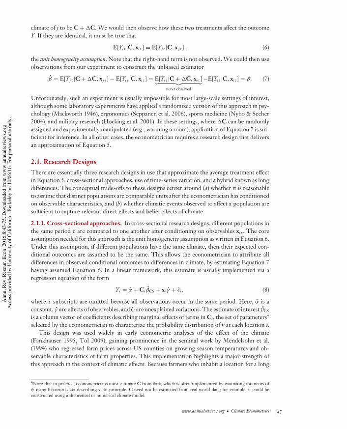
where C2 = C1 + %C. This assumption states that the change in expected outcomes between aperiod where cτ is realized relative to outcomes conditioned on a benchmark climate C1 is thesame as the change in expected outcomes if the distribution characterized by C1 were distortedby adjustments to climate parameters by %C (defined as the difference between the realizedmeasures cτ and the climate values C1) to create a new distribution characterized by C2 (Figure 1).
48 Hsiang
Ann
u. R
ev. R
esou
r. Ec
on. 2
016.
8:43
-75.
Dow
nloa
ded
from
ww
w.a
nnua
lrevi
ews.o
rg A
cces
s pro
vide
d by
Uni
vers
ity o
f Cal
iforn
ia -
Berk
eley
on
10/0
6/16
. For
per
sona
l use
onl
y.

RE08CH04-Hsiang ARI 2 September 2016 8:33
–15 –10 –5 0 5 10 15 20 25 >30
Daily temperatures (˚C)
a Identifying variationfrom a small changein daily temperaturedistribution during τ
C1C1
cτ
cτ – C1C2 – C1
b
dc
–15 –10 –5 0 5 10 15 20 25 >30
Daily temperatures (˚C)
Figure 1Illustration of the marginal treatment comparability assumption, adapted from Deryugina & Hsiang (2014). (a) Expected annualdistribution of daily temperatures for Middlesex County, Massachusetts, a characterization of the climate C1. (b) Black-outlined barsare an example weather summary cτ of temperature realizations during period τ , in the form of a distribution, overlaid on C1.(c) Difference between a climate C2, with structure identical to the realized distribution of weather cτ in panel b, and the initial climateC1 in panel a. (d ) The difference between the realized distribution of weather and the climate, cτ − C1. The marginal treatmentcomparability assumption states that the effect of the change in the weather distribution in panel d is the same as the effect of the changein the climate distribution in panel c.
In other words, marginal treatment comparability assumes that the effect of a marginal changein the distribution of weather (relative to expectation) is the same as the effect of an analogousmarginal change in the climate. Because this assumption has been widely debated, in the followingsubsections I propose a partial test of this assumption and derive some conditions under which itholds exactly.
In a linear framework, this approach is usually implemented using either time-series or paneldata via a regression equation of the form
Yiτ = αi + ciτ βTS + xiτ γ + θ(i )(τ ) + ϵi , (10)
where αi are unit-specific fixed effects that absorb the effect of all time-invariant factors that differbetween units, including unobservables that could not be accounted for in the cross-sectionalresearch design. θ(i )(τ ) are trends in the outcome data, often accounted for using period fixedeffects and/or linear or polynomial time trends, which may be region or unit specific.
This approach was probably first proposed by Huntington (1922, p. 14) who argued, “The idealway to determine the effect of climate would be to take a given group of people and measure theiractivity daily for a long period, first in one climate, and then in another,” and implemented analogsto Equation 10 using factory worker data. This approach gained prominence in modern economicanalysis when used by Deschenes & Greenstone (2007), who analyzed whether agricultural profitsin US counties responded to “random fluctuations in weather.”
The core benefit of this approach is that it accounts for unobservable differences betweenunits, eliminating a potential source of omitted variables bias. However, this approach still remainsvulnerable to omitted variables bias if there are important time-varying factors that influence theoutcome and are correlated over time with ciτ or xiτ after conditioning on trends θ(i )(τ ). It is usuallyassumed that variations in ciτ over time are exogenous to changes in social and economic changesbecause they are driven by stochastic geophysical processes. However, Hsiang (2010) points outthat many dimensions of ciτ are correlated over time because they are partially driven by the sameprocesses—e.g., temperature, rainfall, and hurricanes are all modulated by ENSO—so βTS may bebiased if important climatic variables are omitted. A separate concern raised by Auffhammer et al.
www.annualreviews.org • Climate Econometrics 49
Ann
u. R
ev. R
esou
r. Ec
on. 2
016.
8:43
-75.
Dow
nloa
ded
from
ww
w.a
nnua
lrevi
ews.o
rg A
cces
s pro
vide
d by
Uni
vers
ity o
f Cal
iforn
ia -
Berk
eley
on
10/0
6/16
. For
per
sona
l use
onl
y.
RE08CH04-Hsiang ARI 2 September 2016 8:33
(2013) and Hsiang et al. (2015) is that weather data might not be orthogonal to socioeconomicconditions because weather reporting is endogenous. The extent to which these two issues affectthe literature as a whole remains unknown.
Some authors introduce time-varying nonclimatic factors as controls in Equation 10, such ascrop prices or avoidance behavior. However, Hsiang et al. (2013) caution that this may introducenew biases if these factors are endogenous and affected by climatic events, a situation known asbad control (Angrist & Pischke 2008).
A special case of the time-series research design are cohort analyses, such as those conductedby Maccini & Yang (2009) who examined the long-term effects of rainfall during childhoodamong girls in Indonesia. In these implementations, sequential cohorts within a location i areassumed to be comparable to one another conditional on xiτ , differing only in their exposure tosequential realizations of ciτ . This represents a strengthening of the unit homogeneity assumption,as sequential cohorts within i are different populations that are assumed to be comparable.
2.1.3. A hybrid approach: long differences. An approach that aims to compromise betweenthe strengths and weaknesses of cross-sectional analysis and time-series identification is the long-differences strategy, in which changes for both the outcome and the climate within locationsare correlated across locations. The long-differences strategy is a cross-sectional comparison ofchanges over time, which for two periods of observation {τ1, τ2} is implemented with the regression
Yiτ2 − Yiτ1 = α + (ciτ2 − ciτ1 )βLD + (xiτ2 − xiτ1 )γ + ϵi , (11)
where α represents the secular change in Y over time, and βLD represents the extent to whichtrends in climate are correlated across space with trends in Y. This approach is known as “long”differences because it is primarily used to test whether gradual changes in c induce gradual changesin Y, so τ1 and τ2 are usually chosen to be two periods far apart in time. When long differenceshas been implemented to measure the effects of climate on growth (Dell et al. 2012), crop yields(Burke & Emerick 2016, Lobell & Asner 2003), and conflict (Burke et al. 2015b), authors havefound that βLD is almost identical to βTS, leading them to conclude that gradual changes in c likelyinduce similar effects to more rapid changes in c.
The benefit of using long differences, relative to time-series analyses that use short differences,is that the marginal treatment comparability assumption in Equation 9 might be more plausiblysatisfied because changes in c are gradual—although a weakness of this approach relative to purecross section is that some form of this assumption is still required. The benefit of this approachrelative to pure cross-sectional analyses is that it requires a weaker form of the unit homogeneityassumption, where only changes in Y are assumed to be comparable across units rather thanrequiring levels of Y to be comparable. But this assumption remains stronger than the weakwithin-unit homogeneity assumption required for time-series identification. This tension betweenthe marginal treatment comparability assumption and the unit homogeneity assumption is anoverarching challenge to research design in this literature, as discussed below.
2.2. The Trade-Off Between Low-Frequency Variationsand Credible IdentificationThe extent to which Equation 10 identifies direct effects and belief effects of the climate is oftenthought to depend on the lengths of periods over which the distribution ψ(ciτ ) is summarized,that is t − t. Because belief effects are caused by agents responding to the belief that they facea probability distribution of outcomes described by Ciτ , the extent to which these effects arecaptured by Equation 10 likely depends on an agent’s belief that changes in the distribution of
50 Hsiang
Ann
u. R
ev. R
esou
r. Ec
on. 2
016.
8:43
-75.
Dow
nloa
ded
from
ww
w.a
nnua
lrevi
ews.o
rg A
cces
s pro
vide
d by
Uni
vers
ity o
f Cal
iforn
ia -
Berk
eley
on
10/0
6/16
. For
per
sona
l use
onl
y.
RE08CH04-Hsiang ARI 2 September 2016 8:33
realized measures ciτ reflect changes in the prior probability of those events occurring. It is widelyassumed that agents facing events vi t for long τ will update their beliefs over Ciτ , whereas agentsexperiencing events during a short period—perhaps only for a 5-min period—will not alter theirbeliefs over Ciτ for that interval. Thus, individuals might experience the direct effects of climaticevents during short τ , but they may be unlikely to alter their beliefs about the climate they facebecause of a short-lived event.
Because of this logic, it is widely thought that low-frequency data (long %τ = τ2 − τ1 = t − tfor regularly spaced data) are required to measure belief effects when using time-series variation,as populations only adjust their beliefs if environmental changes are persistent. In the limit thatfrequencies of ciτ exploited by the econometrician approach zero (i.e., the length of%τ approachesinfinity), the research design actually approaches the pure cross-sectional analysis in Equation 8.Thus, the motivation to exploit low-frequency data in time-series designs mirrors the motivation ofcross-sectional analysis, as those data are thought to capture both the direct effects and belief effectsof climate changes. Early examples of this approach are Zhang et al. (2007) and Tol & Wagner(2010), both of whom apply a low-pass filter to climatic variables before estimating Equation 10.A related alternative approach is to use climate data sampled at a low frequency, as implementedby Bai & Kung (2011), who count droughts over each decade to form each observation in amillennial-scale time series.
Although exploiting low-frequency variations in c is appealing because such an approach mightcapture both direct and belief effects, it comes at the cost of less credible identification, an issuehighlighted by Hsiang & Burke (2014, p. 2) as the “frequency-identification trade-off.” The unithomogeneity assumption for time series identification is
E[Yiτ |C, xiτ ] = E[Yi,τ+%τ |C, xi,τ+%τ ], (12)
where units of observation are assumed to be comparable across periods of observation. How-ever, as the frequency (1/%τ ) of observation becomes lower, the assumption that Yiτ and Yi,τ+%τ
are comparable becomes increasingly difficult to justify. For example, populations separated bymultiple centuries might not be comparable units.
The tension between credible identification and use of low-frequency climate variation is noteasily resolved if populations do not update their beliefs about the climate more quickly thanthese populations naturally change in other fundamental ways. For cases in which belief effects arelarge relative to direct effects, then the frequency-identification trade-off may represent a majorchallenge to credible identification of the total effect of the climate. Importantly, however, if theprimary way in which belief effects manifest is to alter the direct effects of the climate—i.e., beliefeffects are mostly adaptations designed to cope with direct effects—then the total effects of climatestill may be nearly identified with high-frequency time series. Even when this condition is notsatisfied, exact identification may still be possible, as shown in Section 2.4.
2.3. A Partial Test of Marginal Treatment ComparabilityUnit homogeneity assumptions can be weakened but never tested or eliminated entirely, a funda-mental limitation in causal inference generally. However, it may be possible to implement a partialtest of the marginal treatment comparability assumption by comparing whether estimated effectsare similar when using approaches that exploit climatic variations at different temporal frequencies.If βCS = βLD = βTS, i.e., if the effects of high-frequency changes equal the effects estimated withlong differences and in cross section, then one possible explanation is that the marginal treatmentcomparability assumption is valid, and temporary changes in realizations of c have similar effects toanalogous changes in C. This could be true if the sum of all belief effects is small on net. Versions
www.annualreviews.org • Climate Econometrics 51
Ann
u. R
ev. R
esou
r. Ec
on. 2
016.
8:43
-75.
Dow
nloa
ded
from
ww
w.a
nnua
lrevi
ews.o
rg A
cces
s pro
vide
d by
Uni
vers
ity o
f Cal
iforn
ia -
Berk
eley
on
10/0
6/16
. For
per
sona
l use
onl
y.
RE08CH04-Hsiang ARI 2 September 2016 8:33
of these different comparisons were implemented and discussed in Burke & Emerick (2016), Burkeet al. (2015b), Dell et al. (2009), Hsiang & Jina (2015), Lobell & Asner (2003), and Schlenker &Roberts (2009), in which any differences in estimated effects were attributed to adaptations toclimate, i.e., belief effects that interact with direct effects. However, a known difficulty is that thestrength of this test relies directly on the validity of the different unit homogeneity assumptionsused in each of the models compared. It is theoretically possible to obtain βCS = βLD = βTS bychance even if all key assumptions are violated, so long as biases have countervailing effects.
Building on these earlier partial tests, I propose that the credibility of this approach can befurther strengthened by estimating climate effects using a spectrum of data that has been filtered atall different temporal frequencies. If the estimated effect of changes in c is stable across all temporalfrequencies spanning from unfiltered time-series data to long differences and the zero-frequencycross section, then it seems less plausible that omitted variables biases at different frequenciesare exactly offsetting belief effects and more plausible that the marginal treatment comparabilityassumption is valid. The idea for this test comes from the observation that a time series of the kthelement of the vector c can be decomposed into the Fourier series
ckτ = ak0 +
∞∑
ω=1
[akω sin(ωτ ) + bk
ω cos(ωτ )], (13)
where akω and bk
ω are constants representing projections onto the basis functions sine and cosineat varying frequencies ω, and ak
0 is a constant, analogous to a long-run average (i.e., ω = 0).Outcome data Y can be similarly decomposed. If we can find appropriate filters that allow us toisolate only certain frequency bands [ω, ω], then we can estimate Equation 10 using these filtereddata and obtain β [ω, ω]
TS , the estimated relationship between climate variables and an outcome ateach timescale. As timescales become longer (and frequencies become lower), this estimate shouldcontinuously approach the long-differences estimate and eventually the cross-sectional estimateif the marginal treatment comparability assumption is valid and these estimates are unbiased.
To demonstrate this test, I obtained panel data on annual county-level maize yield, temperature,and rainfall used in Schlenker & Roberts (2009), updated to the year 2014 and restricted to the 730counties east of the 100th meridian that had no missing observations. I then applied a Baxter-Kingapproximate band-pass filter (Baxter & King 1999) to all three variables for various frequencies andestimated Equation 10 with each set of filtered data. Figure 2 shows the effect of temperature onyields at these various timescales overlaid with estimates of βTS as in Schlenker & Roberts (2009),βLD as in Burke & Emerick (2016), and βCS as in Schlenker et al. (2006). In all cases, except the crosssection, these estimated effects are near one another and not statistically different, suggesting thatvariations in temperature over time have similar effects on maize yields in this context, regardless ofthe timescale of these variations. The uniqueness of the cross-sectional estimate could be explainedeither by belief effects that emerge only at timescales longer than 33 years (the longest timescaleof the filtered data) or omitted variables bias—although the fact that βCS changes substantially(to more closely resemble time-series estimates) when rainfall terms are omitted highlights thevulnerability of the cross-sectional approach to misspecification. Nonetheless, these results overallappear consistent with an assumption of marginal treatment comparability in this context, at leastfor timescales shorter than 33 years.
2.4. Exact Identification of Climate Effects Using Weather VariationWhy should low- and high-frequency variations in climatic variables ever provide comparabletreatments? It is possible that cross-section, time-series, long-difference, and filtered data allprovide similar parameter estimates for β by chance, such that the above test of marginal
52 Hsiang
Ann
u. R
ev. R
esou
r. Ec
on. 2
016.
8:43
-75.
Dow
nloa
ded
from
ww
w.a
nnua
lrevi
ews.o
rg A
cces
s pro
vide
d by
Uni
vers
ity o
f Cal
iforn
ia -
Berk
eley
on
10/0
6/16
. For
per
sona
l use
onl
y.

RE08CH04-Hsiang ARI 2 September 2016 8:33
0 10 20 30 40
10
1950 1962 2002 2014
Year
101
1
1950 1962 2002 2014
Year
2–5
6–9
10–1314–1718–33
Raw
ann
ual d
ata
b d
Chan
ge in
log
annu
al y
ield
s
Temperature during additional 24 h (˚C)
–0.08
–0.04
[9]
[8][7]
[6][1,2,5][3,10]
[4]
0
Filte
red
data
by
peri
odic
ity (y
ears
)a c e
Raw annual (1950–2014) [1] (Schlenker & Roberts 2009)Raw annual (1962–2002) [2]2–5 year period [3]6–9 year period [4]10–13 year period [5]14–17 year period [6]18–33 year period [7]Long difference (1980–2000) [8] (Burke & Emerick 2016)Cross section (1950–2014) [9] (Schlenker et al. 2006)Cross section without rainfall (1950–2014) [10]
BK filtered data (1962–2002)
–0.12
Degree days above 29˚C(Grand Traverse, MI)
Corn yields (bushels/acre)(Grand Traverse, MI)
Change in log annual yields
Figure 2(a–d ) Example outcome and climate time series data from Grand Traverse, Michigan, filtered at different frequencies. (a) Raw annualdegree-days data (black) and a 30-year-long difference (maroon) following Burke & Emerick (2016). (b) The same data decomposed intotime series at different frequencies, where a Baxter-King band-pass filter has been applied for different periodicities. Filtering causesloss of data at the start and end of the time series. (c) Illustrates analogous data as in panel a but for corn yields. (d ) Illustrates analogousdata as in panel b but for corn yields. (e) Comparison of the estimated effect of daily temperature using raw panel data sets, filtered datasets, long differences, and cross-sectional approaches. Sample and estimation indicated by both line and bracketed numbers.
treatment comparability paints a misleadingly consistent picture of climate effects and weathereffects that are not related. Such critiques, relying on heuristic arguments, are common inthe literature. Nonetheless, there is actual theoretical justification for the marginal treatmentcomparability assumption. In this section I provide a new derivation demonstrating how, undercertain conditions, the total effect of climate can be exactly recovered using βTS derived fromweather variation. In essence, this result is a combined application of two well-known results, theEnvelope Theorem and the Gradient Theorem.
The intuition of the result is as follows. Imagine there are two otherwise identical householdsthat are next-door neighbors on a street that runs north–south. The more northern householdfaces a very slightly different climate because it is very slightly further north. The difference inclimate faced by the two households is vanishingly small, but nonzero. These two householdshave the ability to adapt many dimensions of their daily life to their beliefs about their respectiveclimates, and they will adopt slightly different behaviors and investments that maximize variousoutcomes, generating belief effects. However, if we focus on outcomes that are maximized by thehouseholds, then the overall net effect caused by these slightly different adaptation decisions is zerobecause any marginal benefits that the northern household reaps are exactly offset by additionalmarginal costs (which is known because the household is at a maximum). Therefore, any differencein the optimized outcome between the two households must come from the direct effects of theslightly different climate, and the influence of slightly different beliefs and adaptations between thetwo households can be ignored. If a weather realization occurs such that the southern householdexperiences conditions that are slightly different from what they expect, and its distribution ofweather actually matches the climate of the northern household, then this weather effect on the
www.annualreviews.org • Climate Econometrics 53
Ann
u. R
ev. R
esou
r. Ec
on. 2
016.
8:43
-75.
Dow
nloa
ded
from
ww
w.a
nnua
lrevi
ews.o
rg A
cces
s pro
vide
d by
Uni
vers
ity o
f Cal
iforn
ia -
Berk
eley
on
10/0
6/16
. For
per
sona
l use
onl
y.

RE08CH04-Hsiang ARI 2 September 2016 8:33
optimized outcome of the southern household must be exactly the same as the cross-sectional dif-ference across the two households in a year when their weather realizations match their respectiveclimates perfectly. This is because in both cases, there is no influence of changing beliefs on theoptimized outcome. Stated simply, the marginal effect of the climate on an optimized outcome isexactly the same as the marginal effect of the weather.
Based on this insight, we can trace out a curve describing climate effects between sequentialneighbors by watching how optimized outcomes in each household change when that householdis confronted by a weather distribution that matches the climate of their immediate next-doorneighbor. The integral of these marginal differences between sequential neighbors must thendescribe how the climate generates larger differences between households that are not adjacentneighbors and how they experience climates that differ by a nonmarginal amount. Importantly,this integration procedure does not assume that individuals do not adjust their beliefs and adaptto their climate. Rather, the marginal effect of such adjustments for marginal climate changesis zero on an optimized outcome, so marginal effects of weather—which do not cause beliefs tochange—can be used as a substitute for marginal climate changes in the integration, despite thepresence of changing beliefs and adaptations.
To see this result formally, consider an outcome of interest Y that may be affected by theclimate C through its effect on weather realizations c and actions b and which is optimized so itcan be written as a value function, i.e., the solution to a maximization problem over an outcome-generating function z(b, c). If we assume z is differentiable and concave in b, there will be a uniqueoptimum b∗(C) for each climate:
Y (C) = Y [b∗(C), c(C)] = maxb∈RN
z[b, c(C)]. (14)
Recall that the notation c(C) means weather realization c generated from climate C. Note thatmaximization of z is allowed to occur through some indirect process, such as efficient market al-locations, and need not result from explicit maximization by agents. Figure 3a plots the outcomesurface z for an example case in which C, c, and b each have only one dimension. For each valueof C, b∗ is chosen to maximize z so the outcome Y observed is the locus of optima along the redline.
Let C1 be a benchmark climate at which we are evaluating Y(C). If we differentiate Y by thekth element of C, by the chain rule we have
dY (C1)dCk
= ∂z[b∗(C1), c(C1)]∂Ck
+N∑
n=1
∂z[b∗(C1), c(C1)]∂bn
dbn
dCk+
K∑
κ=1
∂z[b∗(C1), c(C1)]∂cκ
dcκdCk
, (15)
where∂z∂Ck
= 0, (16)
because the climate, as summary statistics of a probability distribution, cannot affect any outcomeby a pathway other than through the weather realizations it causes and actions based on beliefsregarding its structure. Because Y is the outcome when z has been optimized through all possibleadaptations, and it is differentiable in b, we also know
∂z[b∗(C1), c(C1)]∂bn
= 0 (17)
for all N dimensions of the action space. Thus, Equation 15 simplifies to
dY (C1)dCk
=K∑
κ=1
∂z[b∗(C1), c(C1)]∂cκ
dcκdCk
=K∑
κ=1
∂Y (C1)∂cκ
dcκdCk
. (18)
54 Hsiang
Ann
u. R
ev. R
esou
r. Ec
on. 2
016.
8:43
-75.
Dow
nloa
ded
from
ww
w.a
nnua
lrevi
ews.o
rg A
cces
s pro
vide
d by
Uni
vers
ity o
f Cal
iforn
ia -
Berk
eley
on
10/0
6/16
. For
per
sona
l use
onl
y.

RE08CH04-Hsiang ARI 2 September 2016 8:33
a b
c d
cc
Y Y
YY
b
z(b,c)
Y(b*(C ),c(C ))
Y(b*(C ),c(C )) z(b*(C1),c(C ))
z(b*(C1),c(C ))
Yi=2(b*(C),c(C ))= ∫∂Y(C)/∂cdC + Φi=2
Yi=1(b*(C),c(C ))= ∫∂Y(C)/∂cdC + Φi=1
Yi=1(C1) + ∂Y(C1)/∂c × (C – C1)
cross sectionY(b*(C1),c(C1))Yi=2(C2) Yi=1(C1)
Yi=1(C2)
∂Y(C1)/∂c
∂Y(C2)/∂c
∂Y(C2)/∂c ∂Y(C1)/∂c
∂Y(C1)/∂c
c(C1)
c(C2)c(C2)
b*(C1) b*(C2) b c
c(C1)
c(C2) c(C1)
Y(b*(C2),c(C2))Y(b*(C2),c(C2))
Figure 3(a) Outcome generating function z(c, b) over weather outcome c(C) that reflects the climate and decision b(C) that responds to beliefsabout the climate. An implicit fourth dimension not pictured is climate C, where we let E[c(C)] = C for simplicity. The red line is thevalue function Y(C), the optimum achieved via maximization over z(.), conditional on a given value for C, which agents cannot control.(b) The rotated view looking at the c-Y plane. Local variations in the outcome due to small changes in weather (blue arrows) are tangentto the locus of optima. (c) Rotated view looking at the b-Y plane. The locus of optima (red line) is achieved because of adaptation tochanges in climate, indicated by shifts in the b dimension. If agents beginning at C1 could not adapt, they would be constrained topoints on the outcome-generating function along the blue line. (d ) This panel shows the same view as panel b. The red line is Y(C) forlocation i = 1. The locus of points along the no-adaptation blue curve (as in panel c) lies below the actual optimum for all values exceptC1. The green line shows extrapolation of the marginal effect of the climate measured at C1. The orange line is Y(C) for location i = 2,where the integration constant φi is different than for i = 1. The black line marks the cross-sectional relationship that would berecovered if Yi=1(C1) and Yi=2(C2) were the sample.
Note that for any marginal change in the distribution of weather, there exists a marginal changein climate that is equal in magnitude and structure such that
dcκdCk
={
1 for κ = k0 otherwise
. (19)
www.annualreviews.org • Climate Econometrics 55
Ann
u. R
ev. R
esou
r. Ec
on. 2
016.
8:43
-75.
Dow
nloa
ded
from
ww
w.a
nnua
lrevi
ews.o
rg A
cces
s pro
vide
d by
Uni
vers
ity o
f Cal
iforn
ia -
Berk
eley
on
10/0
6/16
. For
per
sona
l use
onl
y.

RE08CH04-Hsiang ARI 2 September 2016 8:33
Focusing only on these analogous measures of weather and climate,5 we have
dY (C1)dCk
= ∂Y (C1)∂ck
, (20)
which says that the total marginal effect of the kth dimension of the climate, evaluated at C1,is equal to the partial derivative of the outcome with respect to the same dimension of weather,also evaluated at C1. Locally, the marginal effect of the climate on Y is identical to the marginaleffect of the weather. Equation 20 implies that Equation 9, the marginal treatment comparabilityassumption, holds.
The equivalence between marginal effects of climate and weather can be used to constructestimates for nonmarginal effects of the climate by integrating marginal effects of weather. Foran arbitrary climate C2, we know from the Gradient Theorem that we can solve for Y (C2) bycomputing a line integral of the gradient in Y along a continuous path through the k-dimensionalclimate space from C1 → C2, starting from Y (C1):
Y (C2) =∫ C2
C1
dY (C)dC
· dC + φ =∫ C2
C1
∂Y (C)∂c
· dC + φ =∫ C2
C1
∇cY (C) · dC + φ, (21)
where the substitution from Equation 20 is made for each of the K elements of the gradient vector∇cY (C) = [ ∂Y (C)
∂c1, . . . , ∂Y (C)
∂cK]. Here, φ = Y (C1) is the constant of integration, which is usually
unknown, although, in virtually all applications, changes in Y are the focus of investigation andintegration constants are differenced out. The vector of differentials ∇cY (C) describes all themarginal effects of the weather measured locally at C, which can be estimated empirically byrestricting the sample of observations to those near C and applying Equation 10:
∇cY (C) = βTS
∣∣∣C
. (22)
This estimate can then be substituted into Equation 21 to construct an exactly identified changein Y that occurs as the climate is varied from C1 to C2, in the presence of adaptation adjustmentsin b, using only time-series estimates:
Y (C2) − Y (C1) =∫ C2
C1
βTS
∣∣∣C
· dC. (23)
The difference in outcomes due to a change in the climate is computed by integrating a sequence ofweather-derived marginal effects evaluated at each intermediate value of C. Figure 3b illustratesthis integration along the envelope of the function z(.), and Figure 3c demonstrates how the locusof points along this integration allows for all adaptations to climatic changes that occur throughadjustment of b, reflecting beliefs that evolve with C. As illustrated in Figure 3d, the integral inEquation 23 differs from extrapolation of marginal weather effects (green line) or changes alonga path on the outcome-generating function z(.) where b is held fixed, which would occur if agentswere constrained not to adapt (blue curve).
To summarize, if the outcome is a solution to a maximization problem (Equation 14) for afunction z(.) that is continuous and differentiable in the space of all adaptive actions b, then byapplication of the Envelope Theorem (Equation 18) we know that the marginal effect of the climateis exactly the same as the marginal effect of an equally structured change in the weather distribution(Equation 20), if both are evaluated locally relative to an initial climate. By the Gradient Theoremwe know that a sequence of marginal effects of the weather empirically estimated via time-series
5This focus on the effects of climate and weather where κ = k is consistent with interpreting multiple regression coefficientsas causal effects of Ck when other dimensions of C are fully and simultaneously accounted for.
56 Hsiang
Ann
u. R
ev. R
esou
r. Ec
on. 2
016.
8:43
-75.
Dow
nloa
ded
from
ww
w.a
nnua
lrevi
ews.o
rg A
cces
s pro
vide
d by
Uni
vers
ity o
f Cal
iforn
ia -
Berk
eley
on
10/0
6/16
. For
per
sona
l use
onl
y.

RE08CH04-Hsiang ARI 2 September 2016 8:33
variation at sequential values of C can then be integrated to compute the effect of nonmarginalclimate changes (Equation 23).
Note that this result does not depend on the nature of individuals’ expectations.It is straightforward to extend this result to cases in which the climate exerts direct effects on
the outcome by altering a constraint on a maximization problem, rather than entering througharguments to the maximand (Mas-Colell et al. 1995).
The black curve in Figure 3d demonstrates how a cross-sectional regression, as inEquation 8, may produce different results than the integration of weather effects proposed here.Cross-sectional analysis does not difference out the integration constant φ, so if φi=1 = φi=2 forpairs of observations, then a cross-sectional regression will not recover the red curve. For cross-sectional regressions to recover the effect of C on Y in this context, we require all of the aboveassumptions as well as the additional assumption that integration constants are identical:
dφdi
= 0, (24)
which implies the strong form of the unit homogeneity assumption that units are comparable inlevels conditional on the climate (Equation 6). Thus, the set of assumptions necessary for validcross-sectional identification in this setting is strictly larger than the set of assumptions requiredfor valid time-series identification.
To my knowledge, the above result has not been previously established, and as such, existingempirical papers leveraging weather variation do not explicitly check the assumptions criticalto this result: that Y is the solution to a (constrained) maximization, that adaptations b take oncontinuous values, and that the maximand function z(.) is differentiable in b. Further, many priorstudies do not properly compute climate effects via Equation 23, with the notable exception ofSchlenker et al. (2013) and Houser et al. (2015), who essentially implement a form of this approachexplicitly. Total effects of climatic changes in Equation 23 are also computed correctly in studieswhere marginal effects of weather are allowed to change based on underlying climatic conditions.These evolving marginal weather effects are integrated to compute the cost of shifting climaticconditions, as in Hsiang & Narita (2012) and Burke et al. (2015c). Finally, those studies in whichthe marginal effects of weather are approximately invariant in climate, such as Ranson (2014) andDeryugina & Hsiang (2014), also basically estimate Equation 23 when they linearly extrapolateweather effects because the two calculations are equivalent.
3. MEASUREMENT OF CLIMATE VARIABLESThe measurement of climate variables is a critical methodological step in identifying climateeffects, regardless of the research design used. Early analyses concerned only with measuringwhether climatic factors had a nonzero effect, or the sign of an effect, used simple measuresof climate such as latitude or a single indicator variable that is one if a population is exposedto a predefined event (e.g., a drought) and is zero otherwise. This approach is internally validbut has important limitations that are often underappreciated in the literature. First, coarseclimate measures introduce large measurement errors that will cause attenuation bias, leading tounder-rejection of the null hypothesis. Second, the structure of a dose-response function
E[Y |c] = f (c) (25)
is often of interest. For example, we may be interested in nonlinearities or whether multipledimensions of climate interact in important ways, requiring that measures of climate variablesbe near continuous and multidimensional. Third, if measures of c do not reflect scalable physical
www.annualreviews.org • Climate Econometrics 57
Ann
u. R
ev. R
esou
r. Ec
on. 2
016.
8:43
-75.
Dow
nloa
ded
from
ww
w.a
nnua
lrevi
ews.o
rg A
cces
s pro
vide
d by
Uni
vers
ity o
f Cal
iforn
ia -
Berk
eley
on
10/0
6/16
. For
per
sona
l use
onl
y.

RE08CH04-Hsiang ARI 2 September 2016 8:33
quantities in the real world, we may have little confidence that estimated effects are externallyvalid to other locations or to periods when the climate may change. For example, it is impossibleto consider how cyclone intensification may affect outcomes if cyclone exposure is measured onlyas a binary variable. Fourth, pooling a sample of different locations may provide a valid averagetreatment effect of climatic conditions on the sample, but it may be a poor predictor of outcomesat any actual locations if the physical properties of events coded as similar are not actuallyphysically similar. Finally, the result derived in the previous section, that time-series variationscan be used to exactly identify marginal effects of the climate, can only hold if climatic variationsare measured in such a way that an econometrician can identify marginal effects. For example,binary treatments are not differentiable, and so it may be difficult to determine if changing fromno treatment to treatment is a marginal change.
For all of the above reasons, many of the major innovations covered in the literature over thepast decade have resulted from improvements in the measurement of climate variables, contribut-ing at least as much to recent advances, if not more, than functional form innovations (discussedin Section 4). For example, using spatial interpolation techniques, Schlenker & Roberts (2009)developed estimates of temperature with high spatial and temporal resolution, which allowedthem to construct precise measures of degree-days that integrate cumulative exposure to specifictemperature ranges (Figure 4a). Deschenes & Greenstone (2011) introduced a related approachin which days are counted based on their average temperature [see Deryugina & Hsiang (2014)for a derivation of this approach]. Yang (2008) estimated the effect of tropical cyclones by cod-ing a storm’s maximum windspeed at landfall, an approach enriched further by Nordhaus (2010)and Mendelsohn et al. (2012) who used additional landfall statistics; Hsiang (2010) expandedthe measurement of cyclone exposure by integrating wind speed exposure at all points through-out the lifetime of a storm (Figure 4b). Guiteras et al. (2015) implemented a novel techniquefor detecting surface flooding using satellite imagery. Auffhammer et al. (2006) used an atmo-spheric circulation model to estimate overhead aerosol exposure. Hsiang et al. (2011) developeda method to identify the ENSO exposure of countries (Figure 4c). Fishman (2016) utilized sev-eral metrics to characterize the evenness of rainfall distributions that are similar in total rainfall(Figure 4d ). In several cases, researchers find that established linear or nonlinear transforma-tions of fundamental climatic measures, such as temperature, rainfall, and humidity, are useful inexplaining patterns of outcomes, such as the standardized precipitation evapotranspiration index(Harari & La Ferrara 2013), drought indices (Couttenier & Soubeyran 2014), vapor pressuredeficit (Urban et al. 2015), heat indices (Baylis 2015), or malaria ecology indices (McCord 2016).In all cases, these various measures can be understood as approaches to collapsing the dimen-sionality of c in a manner that efficiently describes patterns that matter from an economic orsocial standpoint. In most of these cases, alternative approaches to measuring climate variablescannot be viewed as objectively wrong; rather there are many ways of describing data in c thatdo not efficiently describe those components of variation that most strongly influence the out-comes of interest. Blunt climate measures are not wrong, they just introduce large measurementerrors.
Particular caution is needed when applying the natural logarithm transformation standard inmany economic applications to climate measures, as it is not always sensible. For example, usinglog(temperature) in Equation 10 is challenging to interpret because a 1% change in temperature—used in the interpretation of the resulting coefficients—has a different meaning depending onwhether temperature is measured in Fahrenheit, Celsius, or Kelvin. In other cases, such trans-formed data can be fit to a model, but the standard interpretation is inconsistent with physicalphenomena. For example, Nordhaus (2010) and Mendelsohn et al. (2012) model hurricane dam-age using log(windspeed) and conclude that damage is superelastic because it appears to grow up to
58 Hsiang
Ann
u. R
ev. R
esou
r. Ec
on. 2
016.
8:43
-75.
Dow
nloa
ded
from
ww
w.a
nnua
lrevi
ews.o
rg A
cces
s pro
vide
d by
Uni
vers
ity o
f Cal
iforn
ia -
Berk
eley
on
10/0
6/16
. For
per
sona
l use
onl
y.

RE08CH04-Hsiang ARI 2 September 2016 8:33
29°C
mm
mm
100
200
0
Daily rainfall in Ahmedabad, Gujarat
0 50 100 150 200
0
100
200
Days (May 1st–Nov 1st)
1996Total rainfall: 642 mmRainy days: 77
2000Total rainfall: 635 mmRainy days: 47
Met
ers p
er se
cond
0
20
40
60
Kilometerseast
Kilometersnorth
Met
ers p
er se
cond
40
20
0200
–200
00
–200
200
Teleconnectedlocations
Tem
pera
ture
Time24 h 24 h
Degree days >29°CTotal wind speed at surface
Tmax
Tmax
Tmin Tmin Tmin
a b
c d
Figure 4Examples of innovations in climate measurement. (a) Construction of degree-days measures using hourly temperature data interpolatedbetween daily minimum and maximum temperature in Schlenker & Roberts (2009). (b) Wind field model used to reconstruct windexposure along the path of tropical cyclones (inset is computed exposure of super typhoon Joan) in Hsiang & Jina (2014).(c) Identification of “teleconnected” pixels (red) that have temperature and rainfall strongly coupled to the El Nino-SouthernOscillation in Hsiang et al. (2011). (d ) Example rainfall distributions used to construct the rainy days count as a measure of within-yearrainfall dispersion across two years with similar total rainfall in Fishman (2016).
six exponents faster than the energy of the storm—a misinterpretation that is readily reconciledwith physics when the log transformation is simply not applied (Camargo & Hsiang 2016).
Many dimensions of the climate, such as persistent drought and sea level, remain poorly cap-tured in econometric models due to measurement challenges. Future innovations will furtherimprove our understanding of these climate effects substantially.
4. ECONOMETRIC MODELSHaving selected a research design and constructed appropriate climate measures, an econometri-cian must select a model that is fitted to the data. Here I discuss five aspects of modeling that have
www.annualreviews.org • Climate Econometrics 59
Ann
u. R
ev. R
esou
r. Ec
on. 2
016.
8:43
-75.
Dow
nloa
ded
from
ww
w.a
nnua
lrevi
ews.o
rg A
cces
s pro
vide
d by
Uni
vers
ity o
f Cal
iforn
ia -
Berk
eley
on
10/0
6/16
. For
per
sona
l use
onl
y.

RE08CH04-Hsiang ARI 2 September 2016 8:33
been particularly important in the measurement of climate effects: nonlinearities, displacement,uncertainty, adaptation, and cross-study comparisons.
The discussion here is focused on the measurement of climate effects by applying a reducedform approach to construct a dose-response surface. Such an approach does not necessarily specifya single pathway through which the climate affects social outcomes, and in many cases it is likelythat several pathways play a role. Hsiang et al. (2013) suggest that to reject potential pathways inany given context, researchers must look for natural experiments in which a particular pathway isobstructed due to external factors and then examine whether reduced form effects persist; studiesby Sarsons (2015) and Fetzer (2014) are useful examples of this strategy.
It is worth noting that a large number of studies in economics utilize variation in weatheras an instrumental variable to study the effect of an intermediary variable on an outcome. Thisstrategy relies on the assumption of an exclusion restriction, i.e., that the employed weathervariation only affects the outcome through the specified intermediary variable. This assumption isuntestable, although the large number of studies utilizing exogenous variation in weather to studya large number of outcomes through various proposed pathways seems to be evidence that thisassumption cannot be true in many cases.
4.1. Nonlinear EffectsThe interpretation and estimation of nonlinear effects depend heavily on whether observationsare highly resolved in space and time or whether they are highly aggregated. Because weatherdata are often available at high resolution, even when outcome data are not, it is often possibleto recover microlevel response functions, below the level of aggregation in the outcome data, bycarefully considering the data generating process.
4.1.1. Recovering local, microlevel, and instantaneous nonlinear effects. Local effects ofclimatic variables are often nonlinear in important ways, such as extreme cold days and extreme heatdays generating excess mortality (Deschenes & Greenstone 2011) or extreme heat hours causingdamage to crop yields (Schlenker & Roberts 2009). In some cases, such as Aroonruengsawat &Auffhammer (2011) and Graff Zivin & Neidell (2014), outcomes are measured at the same dailyfrequency as these nonlinear effects manifest, rendering their measurement straightforward usingstandard techniques. However, in most cases nonlinear effects manifest over timescales (e.g., hours)and spatial scales (e.g., pixels) that are much finer than the periodicity and spatial scale at whichoutcome data are measured (e.g., annually by country). Similarly, local effects may differ betweenmultiple locations within a unit of observation. Despite aggregation of the outcome across spaceand over moments in time, it is possible to recover nonlinear relationships at the spatial andtemporal scale at which climatic data are recorded. Suppose outcome Yiτ is observed over regionsi (e.g., provinces) made up of more finely resolved positions s (e.g., pixels) during intervals of timeτ (e.g., years) comprised of shorter moments t (e.g., days). Let the instantaneous nonlinear effectof climate at a moment and position be f (cs t), which we approximate as a linear combination ofM simple nonlinear functions (e.g., polynomial terms)
f (cs t) ≈ β1 f1(cs t) + β2 f2(cs t) + . . . + βM fM (cs t) =M∑
m=1
βm fm(cs t), (26)
where the βs are constant coefficients. In practice, f(.) has been successfully modeled as anM-piecewise linear function, as in degree-day models; an Mth order polynomial or restrictedcubic spline (Miller et al. 2008, Schlenker & Roberts 2009); interactions between multiple climatemeasures (Urban et al. 2015), options which have efficiency and (local) differentiability benefits;
60 Hsiang
Ann
u. R
ev. R
esou
r. Ec
on. 2
016.
8:43
-75.
Dow
nloa
ded
from
ww
w.a
nnua
lrevi
ews.o
rg A
cces
s pro
vide
d by
Uni
vers
ity o
f Cal
iforn
ia -
Berk
eley
on
10/0
6/16
. For
per
sona
l use
onl
y.

RE08CH04-Hsiang ARI 2 September 2016 8:33
or an M-piecewise constant or “binned” function (Deryugina & Hsiang 2014, Deschenes & Green-stone 2011), a flexible nonparametric option.
Under the assumption of temporal and spatial separability, i.e., that the outcome of interest isa linear sum of f(.) across positions and moments, weighted by the number of affected economicunits gs (e.g., crop fields) at those positions, then the regressions in Equations 8, 10, and 11 aremodified to the form
Yiτ = αi +[∑
s ∈i
∑
t∈τf (cs t)gs
]
+ xiτ γ + θ(i )(τ ) + ϵiτ , (27)
where the index and functions of τ and region effects αi are omitted in the cross-sectional case.Notably, as demonstrated in Welch et al. (2010), the structure of f(.) may differ between subperiodsin τ so that Equation 27 becomes
Yiτ = αi +{
∑
s ∈i
[∑
t∈τa
f a (cs t)gs +∑
t∈τb
f b (cs t)gs
]}
+ xiτ γ + θ(i )(τ ) + ϵiτ , (28)
if τa and τb represent a partition of period τ . Focusing on Equation 27 for simplicity, we cansubstitute the approximation from Equation 26 and interchange the order of summation to obtain
Yiτ ≈ αi +{
∑
s ∈i
∑
t∈τ
[M∑
m=1
βm fm(cs t)gs
]}
+ xiτ γ + θ(i )(τ ) + ϵiτ
= αi +M∑
m=1
βm
[∑
s ∈i
∑
t∈τfm(cs t)gs
]
︸ ︷︷ ︸fmiτ
+xiτ γ + θ(i )(τ ) + ϵiτ (29)
= αi +M∑
m=1
βm fmiτ + xiτ γ + θ(i )(τ ) + ϵiτ ,
which can be estimated with a linear regression using data at the region-period (iτ ) level. Notethat the regressors fmiτ are weighted sums across space and time of the mth nonlinear functionevaluated at locations s and moments t that are not resolved in the outcome data. Estimationof Equation 29 via regression recovers estimates for βm describing the local and instantaneousfunction f(.), even though it uses coarser data.
4.1.2. Nonlinearity in regional summary measures due to local nonlinearities. Many analy-ses do not estimate Equation 29 but instead examine whether nonlinear relationships exist betweensummary statistics of climate data and aggregated outcome data, because constructing f usuallyinvolves highly disaggregated climate data and is therefore challenging. The most common sum-mary statistic of ckiτ , the kth element of ciτ , is a weighted average value over region i and period τ
ckiτ =∑
s ∈i
∑
t∈τcks t gs . (30)
For example, Dell et al. (2012) construct measures of population-weighted average temperatureover entire countries during an entire year. These region-by-period summary statistics may thenbe used to construct regressors in a nonlinear model, such as the Q-order polynomial
Yiτ = αi +Q∑
q=1
βq (ckiτ )q + xiτ γ + θ(i )(τ ) + ϵiτ , (31)
www.annualreviews.org • Climate Econometrics 61
Ann
u. R
ev. R
esou
r. Ec
on. 2
016.
8:43
-75.
Dow
nloa
ded
from
ww
w.a
nnua
lrevi
ews.o
rg A
cces
s pro
vide
d by
Uni
vers
ity o
f Cal
iforn
ia -
Berk
eley
on
10/0
6/16
. For
per
sona
l use
onl
y.

RE08CH04-Hsiang ARI 2 September 2016 8:33
120
150–40
–20
March1997
April1997
Longitude
Latitude
10˚C
0%
30%
20˚C
30˚C
Tem
pera
ture
Crop
land
Annual temperature
slope b1
slope b1
mass m1mass m2
Dailytemperature
Dai
ly im
pact
Ann
ual i
mpa
ct
a
b
c
d
e
Years have different distributions of daily temperature exposure over cropland weights gS.
slope = m1b1 + m2b2slope = m1b1 + m2b2
Figure 5(a) Heterogenous temperatures across locations s within a region are aggregated based on the distribution of units of analysis gs , in thiscase the spatial distribution of croplands (b). This aggregation means that if climate affects outcomes at a highly localized level (c), shiftsin the regional distribution of climatic exposure of gs (d ) will generate an aggregate response to aggregated climate measures that isgenerally smoother (e). Figure adapted from Burke et al. (2015c).
a widely used approach. Equation 31 differs from Equation 29 such that the two approachesshould not recover identical coefficients, even if the microlevel nonlinear data generating processis unchanged. Burke et al. (2015c) demonstrate that the marginal effects recovered in Equation 31should equal the weighted-average marginal effect at the local level (as estimated in Equation 29),averaged across locations and moments, that is associated with a one-unit shift in the distributionof local climatic conditions (Figure 5). Importantly, it is the spatial covariance between weights gs
and climatic conditions within periods of observation that determines how local nonlinear effectsappear in region-level models such as Equation 31. In general, a wider dispersion of conditionsexperienced across locations and moments within a summarized region leads to greater smooth-ing and flattening of the response in Equation 31 relative to the local instantaneous response(Figure 5c–e). Thus, we expect that larger and more heterogenous regions with longer periods ofobservation should produce smoother and flatter responses to summary climate measures, even iflocal nonlinear effects are unchanged.
4.1.3. Global nonlinear effects. The distribution of climatic conditions experienced over timewithin one region often differs substantially from distributions in other regions. In these cases,average marginal effects should differ if response functions are nonlinear. Marginal effects thatchange as a function of mean climate conditions are easily modeled as an interaction betweenaverage climatic conditions and realizations of climatic variables such that
∂Yiτ
∂ciτ= β(ci ), (32)
62 Hsiang
Ann
u. R
ev. R
esou
r. Ec
on. 2
016.
8:43
-75.
Dow
nloa
ded
from
ww
w.a
nnua
lrevi
ews.o
rg A
cces
s pro
vide
d by
Uni
vers
ity o
f Cal
iforn
ia -
Berk
eley
on
10/0
6/16
. For
per
sona
l use
onl
y.

RE08CH04-Hsiang ARI 2 September 2016 8:33
β = α1 + α2T–
T–1 T–2
T–1
T–2
T
Y
T
Y Y
β(T–)β1 β2
ba
T
Y = α0 + (α1 + α2T– ) × T Y = γ0 + γ1T × γ2T 2
c
T
d
PDF of Tat i = 1
Figure 6Different marginal effects β estimated from variation within different locations with different averageclimates (a) may result from an interaction with average climatic conditions (b). In a panel data setting, thiscan be modeled using an interaction (c), where each panel unit is a local linearization of a nonlinear function,or a global nonlinear function can be estimated using the full sample (d ). Abbreviation: PDF, probabilitydistribution function.
as illustrated in Figure 6a,b. Should an underlying global nonlinear response exist, it could berecovered by estimating a single model that is nonlinear in climate variable realizations, witha response surface that is only locally identified by the time-series variation among units thatexperience realizations in the neighborhood of a tangency point (Figure 6c). This is conceptuallyanalogous to integrating Equation 32 to recover the global response surface (Figure 6d ), whichholds exactly as lim ciτ → ci .
4.2. Displacement and DelayIn many contexts, it is plausible that climatic events at moments in the past or at nearby locationsaffect an outcome at a specific time and place, much like the surface of a pond observed at anymoment and location might depend on whether a raindrop disturbed that location or a nearbypoint on the pond surface moments before. When using time-series identification of climateeffects, it is crucial to account for these ripple effects so that a local transient response is notmischaracterized as a persistent effect. Of particular concern is whether climatic events have a neteffect on outcomes, or whether they simply displace outcomes across time and/or space.
www.annualreviews.org • Climate Econometrics 63
Ann
u. R
ev. R
esou
r. Ec
on. 2
016.
8:43
-75.
Dow
nloa
ded
from
ww
w.a
nnua
lrevi
ews.o
rg A
cces
s pro
vide
d by
Uni
vers
ity o
f Cal
iforn
ia -
Berk
eley
on
10/0
6/16
. For
per
sona
l use
onl
y.

RE08CH04-Hsiang ARI 2 September 2016 8:33
All-
caus
e da
ily m
ale
mor
talit
y ra
tefo
llow
ing
tem
pera
ture
exp
osur
e (p
er 1
00,0
00 in
divi
dual
s)
GD
P lo
ss su
rrou
ndin
g cy
clon
e ex
posu
re a
fter
15
year
s (
% p
er m
eter
per
seco
nd)
a b
0 0–400
400–800
800–1,200
1,200–1,600
1,600–2,000
–0.8
–0.6
–0.4
–0.2
0
0.2
0.4
0.6
–0.02
0.00
0 5 10 15 20 25 30
Effect of neighbor’s exposure
Effect of own cyclone exposure
0.02
0.04
0.06
0.08
0.10
Days after temperature exposureDistance from exposed country (km)
Effect of day with mean temperature <30°F
Effect of day with mean temperature >80°F
Figure 7(a) Temporal lag effects of hot and cold days on all causes of male mortality based on data from Deschenes & Moretti (2009). (b) Spatiallag effects of tropical cyclones on own and neighbors’ GDP 15 years after exposure; inset shows example annuli used to construct spatiallags around Haiti. Adapted from Hsiang & Jina (2014).
Thus far, we have only considered contemporaneous effects of the vector ciτ on outcome Yiτ .We now consider the influence of the entire vector field c(s, t) defined across all positions s andmoments t on the outcome Yiτ .
4.2.1. Temporal displacement. A climatic event at time t might bring an event that wouldotherwise occur at time t + 1 forward in time, an effect known as temporal displacement orharvesting. For example, Deschenes & Moretti (2009) highlight the importance of this concept bydemonstrating that many deaths that occur during hot days in the United States would have likelyoccurred within the subsequent two months even in the absence of a hot day; they thus concludethat an effect of a heat wave will influence the timing of deaths within a relatively narrow window,in addition to creating some entirely new deaths (Figure 7a). Mathematically, the signature oftemporal displacement is for periods following a climatic event to have a response that is oppositein sign to the contemporaneous response. A challenge to identifying these lagged effects is thatthe climatic histories of sequential moments overlap, so it may not be the case that outcomes atany moment are only a response to a single historical climate event. Rather, outcomes at eachmoment represent a superposition of many historical events each at a different moment in time.This issue can be resolved by conditioning expected outcomes on the complete history of climaticevents using a distributed lag model:
Yiτ = αi +L∑
l=0
(ci,τ−l βl
)+ xiτ γ + θ(i )(τ ) + ϵiτ , (33)
where l is a lag length measured in periods (l = 0 indicates a contemporaneous observation),and the maximum lag length considered is L. The identifying assumption to this approach isthat the influence of a climate event at τ0 on outcomes at τ1 is determined by the length oftime τ1 − τ0 separating the observations. As written, this model also assumes additive separabilitybetween lagged effects, although this assumption can be relaxed by interacting lagged terms. It issomewhat standard in the literature to sometimes include negative lags (leads) in Equation 33 as a
64 Hsiang
Ann
u. R
ev. R
esou
r. Ec
on. 2
016.
8:43
-75.
Dow
nloa
ded
from
ww
w.a
nnua
lrevi
ews.o
rg A
cces
s pro
vide
d by
Uni
vers
ity o
f Cal
iforn
ia -
Berk
eley
on
10/0
6/16
. For
per
sona
l use
onl
y.
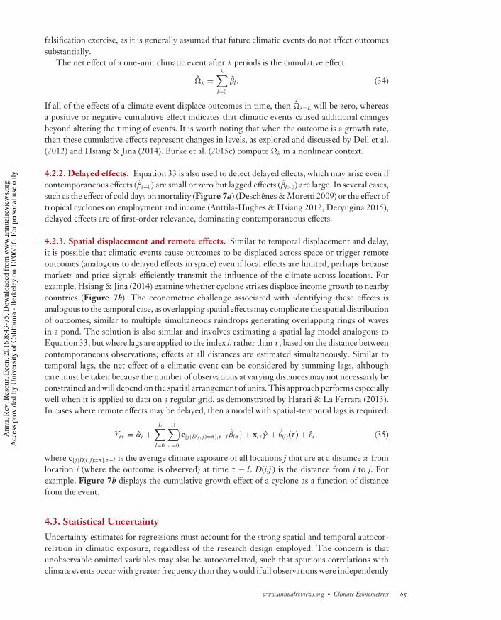
RE08CH04-Hsiang ARI 2 September 2016 8:33
falsification exercise, as it is generally assumed that future climatic events do not affect outcomessubstantially.
The net effect of a one-unit climatic event after λ periods is the cumulative effect
.λ =λ∑
l=0
βl . (34)
If all of the effects of a climate event displace outcomes in time, then .λ=L will be zero, whereasa positive or negative cumulative effect indicates that climatic events caused additional changesbeyond altering the timing of events. It is worth noting that when the outcome is a growth rate,then these cumulative effects represent changes in levels, as explored and discussed by Dell et al.(2012) and Hsiang & Jina (2014). Burke et al. (2015c) compute .λ in a nonlinear context.
4.2.2. Delayed effects. Equation 33 is also used to detect delayed effects, which may arise even ifcontemporaneous effects (βl=0) are small or zero but lagged effects (βl>0) are large. In several cases,such as the effect of cold days on mortality (Figure 7a) (Deschenes & Moretti 2009) or the effect oftropical cyclones on employment and income (Anttila-Hughes & Hsiang 2012, Deryugina 2015),delayed effects are of first-order relevance, dominating contemporaneous effects.
4.2.3. Spatial displacement and remote effects. Similar to temporal displacement and delay,it is possible that climatic events cause outcomes to be displaced across space or trigger remoteoutcomes (analogous to delayed effects in space) even if local effects are limited, perhaps becausemarkets and price signals efficiently transmit the influence of the climate across locations. Forexample, Hsiang & Jina (2014) examine whether cyclone strikes displace income growth to nearbycountries (Figure 7b). The econometric challenge associated with identifying these effects isanalogous to the temporal case, as overlapping spatial effects may complicate the spatial distributionof outcomes, similar to multiple simultaneous raindrops generating overlapping rings of wavesin a pond. The solution is also similar and involves estimating a spatial lag model analogous toEquation 33, but where lags are applied to the index i, rather than τ , based on the distance betweencontemporaneous observations; effects at all distances are estimated simultaneously. Similar totemporal lags, the net effect of a climatic event can be considered by summing lags, althoughcare must be taken because the number of observations at varying distances may not necessarily beconstrained and will depend on the spatial arrangement of units. This approach performs especiallywell when it is applied to data on a regular grid, as demonstrated by Harari & La Ferrara (2013).In cases where remote effects may be delayed, then a model with spatial-temporal lags is required:
Yiτ = αi +L∑
l=0
/∑
π=0
{c[ j |D(i, j )=π ],τ−l βlπ } + xiτ γ + θ(i )(τ ) + ϵi , (35)
where c[ j |D(i, j )=π ],τ−l is the average climate exposure of all locations j that are at a distance π fromlocation i (where the outcome is observed) at time τ − l . D(i,j ) is the distance from i to j. Forexample, Figure 7b displays the cumulative growth effect of a cyclone as a function of distancefrom the event.
4.3. Statistical UncertaintyUncertainty estimates for regressions must account for the strong spatial and temporal autocor-relation in climatic exposure, regardless of the research design employed. The concern is thatunobservable omitted variables may also be autocorrelated, such that spurious correlations withclimate events occur with greater frequency than they would if all observations were independently
www.annualreviews.org • Climate Econometrics 65
Ann
u. R
ev. R
esou
r. Ec
on. 2
016.
8:43
-75.
Dow
nloa
ded
from
ww
w.a
nnua
lrevi
ews.o
rg A
cces
s pro
vide
d by
Uni
vers
ity o
f Cal
iforn
ia -
Berk
eley
on
10/0
6/16
. For
per
sona
l use
onl
y.

RE08CH04-Hsiang ARI 2 September 2016 8:33
distributed—this will cause bias in estimates of standard errors even though estimated climate ef-fects β may be unbiased (Bertrand et al. 2004, Moulton 1986). The extent of the bias in standarderrors depends on the spatial scale and sampling frequency of the data relative to natural patternsof autocorrelation in the climatic variations of interest. Data that are aggregated to large scalesare generally less problematic, and different solutions come at different computational cost andmay be appropriate in different contexts. Schlenker & Roberts (2009) propose applying Conleyspatial standard errors (Conley 1999) that nonparametrically estimate the variance-covariancematrix of β by estimating cov(ϵi,τ , ϵ j,τ ) using ξ [D(i, j )]ϵi,τ ϵ j,τ , where ξ [D(i, j )] is a kernel functionthat weights these terms based on D(i,j), the distance between observations i and j. Hsiang (2010)combines this approach with Newey-West heteroskedastic6 and auto-correlation robust (HAC)standard errors (Newey & West 1987) to also account for temporal autocorrelation within panelunits. Hsiang & Jina (2014) demonstrate that this spatial-HAC adjustment was correctly sized inone context by estimating pseudoexact p-values via randomizing their data in multiple dimensionsand reestimating their model many times. Fetzer (2014) expands this approach to an instrumentalvariables context.
The spatial-HAC approach is computationally intensive, as distances between every pair ofobservations must be computed and transformed, and it does not guarantee a positive-definiteestimate for the covariance matrix of residuals. Thus, it may often be reasonable to estimateapproximate standard errors using simpler techniques, verifying that spatial-HAC adjustmentsdo not alter the result substantively. For example, Dell et al. (2012) simply cluster their standarderrors within panel units to account for temporal autocorrelation. Burke & Emerick (2016) clusterstandard errors for county-level observations in a long-differences model by state to account forwithin-state spatial correlation; cross-state residual correlations in errors are assumed to be smallafter conditioning on state fixed effects. Hsiang et al. (2013) employ a block bootstrap in a fullynonparametric regression and block-resample entire cross sections of a panel data set to account forspatial autocorrelation among contemporary observations. Hsiang et al. (2011) collapse a globalpanel to a single time series when examining ENSO effects, as the treatment generates spatialcorrelations at continental (or larger) scales.
It remains an open question what the most general and efficient approach to estimating statis-tical uncertainty is in most climate econometrics applications. For example, what is the optimalselection of kernel-weighting functions for contemporaneous and serial observations in the spatial-HAC approach? Also, many climate data sets are derived from gridded data, which themselvesmight be spatially interpolated from station data or augmented with a physics-based model—suchas reanalysis products (Auffhammer et al. 2013)—and it remains unknown how these proceduresinfluence the statistical uncertainty of resulting parameter estimates.
4.4. AdaptationAs discussed above, climate affects economic outcomes through belief effects and direct effects,and it is generally thought that most belief effects are adjustments that individuals make to copewith their expected distribution of direct effects. For this reason, belief effects are often describedas adaptations to a climate, although this need not always be true (e.g., beliefs about the climatecould serve simply as a coordinating mechanism). In this framework, adaptations can be definedas belief effects that interact with direct effects; for example, some agents believe it will be coldsometimes at a location, causing them to purchase coats (a belief effect), which reduces the chance
6Note that the Conley approach employed by Schlenker & Roberts (2009) was also robust to heteroskedasticity.
66 Hsiang
Ann
u. R
ev. R
esou
r. Ec
on. 2
016.
8:43
-75.
Dow
nloa
ded
from
ww
w.a
nnua
lrevi
ews.o
rg A
cces
s pro
vide
d by
Uni
vers
ity o
f Cal
iforn
ia -
Berk
eley
on
10/0
6/16
. For
per
sona
l use
onl
y.

RE08CH04-Hsiang ARI 2 September 2016 8:33
they become ill after cold days (a direct effect). Multiple approaches have been used to documentand quantify these adaptations.
4.4.1. Indirect measurement via a cross section of levels. One strategy for measuring theinfluence of adaptations is to estimate the effect of climate on some outcome that is influencedby adaptation using a cross-sectional research design (Equation 8). The central benefit of thisapproach is that it captures all belief effects, including adaptations that interact with direct effectsof the climate. For example, farm prices in Mendelsohn et al. (1994) should reflect any effectsthat beliefs over C have, including the net present value of all future revenues that result fromrealizations of c, which are mediated by these beliefs and the resulting management practices.There are two weaknesses to measuring adaptations using this approach: Measurement relies onthe strongest form of the unit homogeneity assumption (Equation 6), and the cross-sectionalapproach cannot separately disentangle belief effects that do not interact with direct effects, beliefeffects that do, and the integrated effect of all direct effects. However, an approach proposed byMoore & Lobell (2014) combines this approach with time-series identification in an effort topartially isolate these effects from one another.
4.4.2. Explicit observation of adaptation. Another approach to documenting adaptations is toestimate the effect of climate directly on outcomes that are known (or thought) to be adaptationsto climate. For example, Hornbeck (2012) and Hidalgo et al. (2010) estimate the effect of droughton migration of agricultural households, and Kurukulasuriya & Mendelsohn (2008) measure howclimate influences the selection of crops that farmers choose to plant. This approach can be adoptedin a cross-section, times-series, or long-differences framework. A benefit is that the adaptive actionis known and observed directly, rather than indirectly. However, a limitation is that this approachdoes not recover the overall effectiveness of these adaptations, i.e., the extent to which the alteredactions interact with direct effects of climate.
4.4.3. Measurement of implicit adaptation combining time-series variation with stratifi-cation. The one approach able to isolate the effectiveness of adaptations is to use a time-seriesresearch design (Equation 10) for an outcome affected by adaptation, stratifying the sample—orestimating interactions—using variables that are thought to predict the extent of adaptation. Forexample, Auffhammer & Aroonruengsawat (2011) estimate the effect of daily temperature on en-ergy consumption while stratifying by long-run average temperatures, demonstrating that energydemand is higher on hot days in counties that are usually hotter on average. This result suggests thatthe adoption of air conditioning, which is unobserved but assumed to be higher in counties that arehotter on average, increases the effect of temperature on electricity demand. Roberts & Schlenker(2011) effectively stratify a panel of counties by year, implemented by interacting a response func-tion with a nonlinear trend, to understand if innovation over time or learning reduced the heatsensitivity of maize in Indiana [Lobell et al. (2014) ask a similar question by examining how cross-sectional estimates of climatic effects on yields evolve over a sequence of years]. Hsiang & Narita(2012) derive a theory describing when such stratification works to reveal the total effectiveness ofadaptations. According to these authors, a benefit of this approach is its ability to measure the over-all net effectiveness of all adaptive actions that project onto the interacted proxy variables, whereasa weakness is that the costs of indirectly observed adaptations are unknown. To partially addressthis weakness, Schlenker et al. (2013) propose an approach to measure adaptation costs in terms ofthe outcome variable, although it is possible that additional costs or benefits may be unobserved.
Another key challenge of this approach is that those measures used as correlates for adaptations,such as income (Hsiang & Narita 2012), urban status (Burgess et al. 2014), historical experience
www.annualreviews.org • Climate Econometrics 67
Ann
u. R
ev. R
esou
r. Ec
on. 2
016.
8:43
-75.
Dow
nloa
ded
from
ww
w.a
nnua
lrevi
ews.o
rg A
cces
s pro
vide
d by
Uni
vers
ity o
f Cal
iforn
ia -
Berk
eley
on
10/0
6/16
. For
per
sona
l use
onl
y.

RE08CH04-Hsiang ARI 2 September 2016 8:33
with climatic events (Hsiang & Jina 2014), or access to crop insurance (Annan & Schlenker 2015)are not exogenous and vary primarily in cross section. This means it may be difficult to determinewhether changes to the measured variable are a cause of adaptation, an effect of adaptation, ordriven by an omitted variable that determines both. This drawback can be partially solved in caseswhere plausibly exogenous circumstances change an influential factor, enabling a researcher tomore credibly identify whether a specific factor constrains adaptation. This approach is applied byHornbeck & Keskin (2015) to estimate the effect of groundwater discovery on agricultural adap-tation and by Barreca et al. (2013) to estimate the effect of residential air conditioning technologyon health-related adaptation.
4.5. Comparisons and Synthesis of Results Across StudiesUnlike many other econometric studies, such as those that study policy changes, regressors in cli-mate econometric studies are generally physical quantities that have similar or identical meaningat all times and at any location on the planet. Because of this, comparisons across contexts arethought to have clearer interpretations, often demonstrating replicability or highlighting impor-tant differences across samples. For example, Hsiang & Narita (2012) and Hsiang & Jina (2014)demonstrate notable global uniformity in the response to cyclones. In some cases, such as Guoet al. (2014) examining mortality and Hsiang et al. (2013) examining social conflict, standardizationof c to a z-score based on historical variance brings parameter estimates into alignment—perhapsbecause populations form beliefs and adapt effectively to distributions of historical conditions.
In some sectors, notably agricultural impacts and climatic effects on social conflict, explicitcomparisons of seemingly contradictory findings have generated substantial controversy. In thecase of agriculture, much of this disagreement can be reconciled by accounting for inconsistentaggregation of data in the presence of local nonlinearities (see Section 4.1). In the case of socialconflict, much of this disagreement can be reconciled by accounting for statistical uncertainty inparameter estimates (Hsiang & Meng 2014, Hsiang et al. 2015).
Hierarchical meta-analysis has played a role in synthesizing generalizable findings and quan-tifying the extent of agreement in the literature (Hsiang et al. 2013) as well as in constructingcomposite estimates for use in the climate projections discussed below (Houser et al. 2015). Theseapproaches do not assume globally uniform effects but instead model parameter estimates from theliterature in a random-effects framework, where populations experience different true effects ofthe climate but may exhibit a generalizable component that is common across populations (Burkeet al. 2015b, Gelman et al. 2004).
5. ATTRIBUTION AND PROJECTIONTwo objectives of understanding the effect of climate on societies are to understand what ele-ments of the modern world might be attributable to climatic factors and to inform projections offuture outcomes under different climate scenarios. Both are cases in which parameters recoveredempirically are put to work. Note that in the following, I retain only the time index for simplicity.
5.1. Historical AttributionHaving identified the effect of current and previous climatic conditions C on outcome Y, it isnatural to ask, what counterfactual outcomes would we have observed historically under a differentclimate? In our one realization of history, we observed Yt and Ct and estimated a response surfacef (C) that described deviations from some benchmark outcome Y0 associated with the benchmark
68 Hsiang
Ann
u. R
ev. R
esou
r. Ec
on. 2
016.
8:43
-75.
Dow
nloa
ded
from
ww
w.a
nnua
lrevi
ews.o
rg A
cces
s pro
vide
d by
Uni
vers
ity o
f Cal
iforn
ia -
Berk
eley
on
10/0
6/16
. For
per
sona
l use
onl
y.

RE08CH04-Hsiang ARI 2 September 2016 8:33
climate C0. In estimation, these benchmark levels are usually nuisance parameters absorbed byvarious fixed effects, trends, and controls. Observed outcomes are then
Yt = Y0 + f (Ct) − f (C0), (36)
where Y0 can be solved for but is not observed. Writing an analogous equation for an arbitrarycounterfactual climate Ct + %Ct and an associated unknown counterfactual outcome Yt + %Yt ,we difference these equations to obtain
%Yt = f (Ct +%Ct) − f (Ct), (37)
which allows us to estimate %Yt , the alteration of an outcome that we would expect due to achange in historical climate by %Ct . This approach was used by Lobell et al. (2011) to estimatethe historical effect of observed warming on global crop yields, by Hsiang et al. (2011) to estimatethe historical influence of ENSO on global conflict, by Hsiang & Jina (2014) to estimate historicalinfluence of tropical cyclones on national income trajectories, and by Carleton & Hsiang (2016)to attribute impacts based on a variety of results from the literature. Importantly, these estimatesshould be viewed as partial equilibrium estimates insofar as f (.) captures a partial equilibrium re-sponse. Costinot et al. (2016) and Desmet & Rossi-Hansberg (2015) demonstrate more structuredapproaches that can be used to attribute historical impacts in a general equilibrium framework.
Application of Equation 37 must be implemented cautiously, as counterfactual outcomes arenot observed and thus cannot be verified. One indirect test of this approach, useful when f (.) isidentified via time-series variation, is to examine how closely predictions from Equation 37 matchhistorical cross-sectional patterns. Dell et al. (2009) run such a test for effects of temperatureon income, arguing that adaptation and growth convergence must explain the difference. GraffZivin et al. (2015) arrive at similar conclusions when comparing time-series estimates with longdifferences in measures of human capital. Hsiang & Jina (2015) compare predictions based onmicrolevel estimates with macrolevel cross sections for tropical cyclone impacts and concludethat results are largely consistent. In a remarkable higher-order test, Barreca et al. (2015) find thatcross-sectional variation in the intra-annual variance in temperature, when applied to Equation 37,is a good predictor of cross-sectional patterns of intra-annual variance in birth rates.
5.2. Projecting Future Effects of Climate ChangesProjecting impacts of climate changes is analogous to applying Equation 37, except that Ct isreplaced with a benchmark future scenario—usually a “no change” scenario based on historicaldistributions of variables—and%Ct is an anthropogenic alteration to the climate. Early economicanalyses used simple, spatially uniform, general estimates of %Ct , such as imposing a flat +5◦Fwarming and +8% rainfall across the United States (Mendelsohn et al. 1994). In the econometricsliterature, Schlenker et al. (2006) and Deschenes & Greenstone (2007) introduce the use of spatiallyand temporally resolved global climate model simulations to construct %Ct . Lobell et al. (2008)and Burke et al. (2009) demonstrate that when applying climate model projections in Equation 37,accounting for climate model uncertainty in%Ct may be as important as accounting for statisticaluncertainty in f (.) See Burke et al. (2015a) for additional exploration of this issue.
The above approaches generally assume that f (.) has a fixed structure throughout the durationof the projection simulation, perhaps a reasonable assumption in cases where historical changes inf (.) have been limited. However, as demonstrated in Section 2.4 (recall Figure 3d ), the marginaleffect of climate identified via weather and captured in f (.) may become increasingly incorrectas climatic conditions deviate from baseline conditions during a projection simulation and theseadaptations [or other factors, such as those described in Lobell et al. (2014)] alter f (.). To partially
www.annualreviews.org • Climate Econometrics 69
Ann
u. R
ev. R
esou
r. Ec
on. 2
016.
8:43
-75.
Dow
nloa
ded
from
ww
w.a
nnua
lrevi
ews.o
rg A
cces
s pro
vide
d by
Uni
vers
ity o
f Cal
iforn
ia -
Berk
eley
on
10/0
6/16
. For
per
sona
l use
onl
y.

RE08CH04-Hsiang ARI 2 September 2016 8:33
address this issue, Houser et al. (2015) demonstrate how multiple empirical estimates, capturingboth cross-sectional heterogeneity and trends in f (.), could be combined to construct projectionswhere f (.) evolves throughout the projection simulation to reflect historical patterns and rates ofadaptation.
5.2.1. Top-down and bottom-up approaches. Optimal climate policy requires understandingthe full economic burden of potential climate trajectories. Empirical estimates can be used to gen-erate projections of this total cost using either a top-down estimate, where the modeled outcomeYt is some aggregate proxy for well-being, such as GDP (Burke et al. 2015c, Dell et al. 2012,Deryugina & Hsiang 2014, Nordhaus 2006), or constructing bottom-up estimates for multipleoutcomes representing different sectors of the economy that are modeled and summed, sometimescalled the enumerative approach (Houser et al. 2015, Tol 2002). In principle, both approachescan be comprehensive, so long as top-down estimates are augmented with nonmarket impacts. Inpractice, bottom-up estimates may better account for the distributional costs of climate change(Houser et al. 2015), although it is theoretically possible for them to perform equally well. Whenapplying Equation 37 to bottom-up projections, it is important to account for the covariance ofimpacts across different sectors to accurately construct the distribution of aggregate losses (Houseret al. 2015), an effect that is thought to be mostly captured in the estimated responses used fortop-down projections.
6. REMAINING CHALLENGESIn addition to challenges described in the sections above, there are four major areas where I seemethodological innovation as necessary and likely to be successful in the near future.
6.1. Matching Effects and MechanismsRegardless of the research design, most estimated effects of climate are reduced from estimatesthat capture influences on an outcome through all possible pathways. Developing strategies andtechniques that can isolate and characterize a specific mechanism is critical for understandingwhy climatic factors matter. Testing for interactions with potential mediating factors that areplausibly exogenous (Barreca et al. 2013), exploiting natural experiments where specific pathwaysare shut down (Fetzer 2014), and matching detailed patterns of climate influence on outcomes andpotential mediating factors (Anttila-Hughes & Hsiang 2012) are all approaches that have beensomewhat successful in specific contexts, although additional innovations in this area are needed,as these strategies are not always available.
6.2. Adaptation and General EquilibriumAs discussed above, adaptation to climate is thought to be economically important, but it has onlybeen characterized in a limited number of cases. Notably, the costs of adaptations are almost nevermeasured because they are usually not observed. Moreover, most measurements are partial equi-librium responses, whereas general equilibrium responses to climate, such as factor reallocationsacross space or time, are a form of adaptation thought to be important but about which little isknown. Further, general equilibrium changes will result in changing prices, and knowing theseadjustments is important for valuing quantity effects that are already understood. However, onlya small number of studies have begun exploring these effects (Colmer 2016, Costinot et al. 2016,Roberts & Schlenker 2013).
70 Hsiang
Ann
u. R
ev. R
esou
r. Ec
on. 2
016.
8:43
-75.
Dow
nloa
ded
from
ww
w.a
nnua
lrevi
ews.o
rg A
cces
s pro
vide
d by
Uni
vers
ity o
f Cal
iforn
ia -
Berk
eley
on
10/0
6/16
. For
per
sona
l use
onl
y.

RE08CH04-Hsiang ARI 2 September 2016 8:33
6.3. Unprecedented EventsIn analyses of future climate changes, evaluating events that are unprecedented in recent historyis a major obstacle, and any empirical progress on these questions would be highly valuable.Innovative strategies that can measure potential costs of unprecedented physical events, such asrapid sea level rise or ocean acidification, or that characterize the likelihoods of unprecedentedsocial responses to climatic changes, such as mass migrations or state failures, are needed if theseimpacts are to be accounted for systematically in assessment exercises.
6.4. Integration with Theory and Numerical ModelsNumerous theoretical models, including many used for integrated assessment policy analysis,have elements that describe climatic influence on economies (Nordhaus 1993, Stern 2006, Tol2002) but are generally not based on empirically derived relationships. Incorporation of empiricalparameter estimates into process models (Houser et al. 2015, Lobell et al. 2013) and integratedassessment models (Kopp et al. 2013, Moore & Diaz 2015) demonstrates promise, although muchinnovation is needed if these theoretical models are to perform as well as analogous models in otherscientific fields. For example, it is unknown if empirical calibration improves the out-of-sampleforecast performance of these models or if all model parameters are even theoretically estimableusing existing techniques.
7. CONCLUSIONRecent years have seen rapid innovation in the methods used to identify climatic influences oneconomies, with correspondingly rapid growth of insights that are reshaping how we understandthe breadth and importance of climate–society interactions (Carleton & Hsiang 2016, Dell et al.2014). Key innovations have been in research design, the measurement of climatic factors, andthe formulation of econometric models. In sharp contrast to the folk wisdom that “climate is notweather,” here I demonstrate that under fairly general conditions, weather variation, as it is used inmany recent studies, exactly identifies the effect of climate—although many studies to date have notproperly computed the effect of climatic changes when using these weather-derived parameters.Aggregation and synthesis of econometric findings have demonstrated a striking replicability ofmany recent findings across contexts, lending credibility both to the techniques that generatethese results and to exercises where these results are applied to simulations of recent history orfuture climate changes. Many first-order partial equilibrium results are now well understood, yetmajor methodological innovations are still required to (a) tackle the key challenges of identifyingmechanisms, (b) measure adaptation costs, general equilibrium, and price responses, (c) evaluatethe effects of unprecedented events, and (d ) more deeply integrate with theoretical and numericalpolicy models.
DISCLOSURE STATEMENTThe author is not aware of any affiliations, memberships, funding, or financial holdings that mightbe perceived as affecting the objectivity of this review.
ACKNOWLEDGMENTSI thank David Anthoff, Jesse Anttila-Hughes, Max Auffhammer, Alan Barrecca, Marshall Burke,Tamma Carleton, Olivier Deschenes, Tatyana Deryugina, Ram Fishman, Michael Greenstone,
www.annualreviews.org • Climate Econometrics 71
Ann
u. R
ev. R
esou
r. Ec
on. 2
016.
8:43
-75.
Dow
nloa
ded
from
ww
w.a
nnua
lrevi
ews.o
rg A
cces
s pro
vide
d by
Uni
vers
ity o
f Cal
iforn
ia -
Berk
eley
on
10/0
6/16
. For
per
sona
l use
onl
y.

RE08CH04-Hsiang ARI 2 September 2016 8:33
Michael Hanemann, Wu-Teh Hsiang, Bob Kopp, David Lobell, Gordon McCord, Kyle Meng,Billy Pizer, James Rising, Michael Roberts, Wolfram Schlenker, Christian Traeger, and seminarparticipants at Berkeley and Harvard for discussions and suggestions. I thank Wolfram Schlenkerfor generously sharing data.
LITERATURE CITED
Albouy D, Graf W, Kellogg R, Wolff H. 2010. Aversion to extreme temperatures, climate change and quality oflife. Work. Pap., Univ. Mich., Ann Arbor, MI
Angrist JD, Pischke JS. 2008. Mostly Harmless Econometrics: An Empiricist’s Companion. Princeton, NJ: PrincetonUniv. Press
Annan F, Schlenker W. 2015. Federal crop insurance and the disincentive to adapt to extreme heat. Am. Econ.Rev. 105:262–66
Anttila-Hughes JK, Hsiang SM. 2012. Destruction, disinvestment, and death: economic and human losses followingenvironmental disaster. Work. Pap., Univ. San Francisco
Aroonruengsawat A, Auffhammer M. 2011. Impacts of climate change on residential electricity consumption:evidence from billing data. In The Economics of Climate Change: Adaptations Past and Present, ed. GDLibecap, RH Steckel, pp. 311–42. Chicago: Univ. Chicago Press
Auffhammer M, Aroonruengsawat A. 2011. Simulating the impacts of climate change, prices and populationon California’s residential electricity consumption. Clim. Change 109:191–210
Auffhammer M, Hsiang S, Schlenker W, Sobel A. 2013. Using weather data and climate model output ineconomic analyses of climate change. Rev. Environ. Econ. Policy 7:181–98
Auffhammer M, Mansur ET. 2014. Measuring climatic impacts on energy consumption: a review of theempirical literature. Energy Econ. 46:522–30
Auffhammer M, Ramanathan V, Vincent JR. 2006. Integrated model shows that atmospheric brown cloudsand greenhouse gases have reduced rice harvests in India. PNAS 103:19668–72
Auffhammer M, Schlenker W. 2014. Empirical studies on agricultural impacts and adaptation. Energy Econ.46:555–61
Bai Y, Kung J. 2011. Climate shocks and Sino-nomadic conflict. Rev. Econ. Stat. 93:970–81Barreca A, Clay K, Deschenes O, Greenstone M, Shapiro JS. 2013. Adapting to climate change: the remarkable
decline in the US temperature-mortality relationship over the 20th century. NBER Work. Pap. 18692Barreca A, Deschenes O, Guldi M. 2015. Maybe next month? Temperature shocks, climate change, and dynamic
adjustments in birth rates. NBER Work. Pap. 21681Baxter M, King RG. 1999. Measuring business cycles: approximate band-pass filters for economic time series.
Rev. Econ. Stat. 81:575–93Baylis P. 2015. Temperature and temperament: evidence from a billion tweets. Work. Pap. 265, Energy Inst., Univ.
Calif., Berkeley, CABertrand M, Duflo E, Mullainathan S. 2004. How much should we trust differences-in-differences estimates?
Q. J. Econ. 119:249–75Burgess R, Deschenes O, Donaldson D, Greenstone M. 2014. The unequal effects of weather and climate change:
evidence from mortality in India. Work. Pap., London Sch. Econ., LondonBurke M, Dykema J, Lobell DB, Miguel E, Satyanath S. 2015a. Incorporating climate uncertainty into esti-
mates of climate change impacts. Rev. Econ. Stat. 97:461–71Burke M, Emerick K. 2016. Adaptation to climate change: evidence from US agriculture. Am. Econ. J. Econ.
Policy 8(3):106–40Burke M, Hsiang SM, Miguel E. 2015b. Climate and conflict. Annu. Rev. Econ. 7:577–617Burke M, Hsiang SM, Miguel E. 2015c. Global non-linear effect of temperature on economic production.
Nature 527:235–39Burke M, Miguel E, Satyanath S, Dykema J, Lobell D. 2009. Warming increases the risk of civil war in Africa.
PNAS 106:20670Camargo SJ, Hsiang SM. 2016. Tropical cyclones: from the influence of climate to their socioeconomic
impacts. In Extreme Events: Observations, Modeling, and Economics, ed. M Chavez, M Ghil, J Urrutia-Fucugauchi, pp. 303–42. Washington, DC: AGU/Wiley
72 Hsiang
Ann
u. R
ev. R
esou
r. Ec
on. 2
016.
8:43
-75.
Dow
nloa
ded
from
ww
w.a
nnua
lrevi
ews.o
rg A
cces
s pro
vide
d by
Uni
vers
ity o
f Cal
iforn
ia -
Berk
eley
on
10/0
6/16
. For
per
sona
l use
onl
y.

RE08CH04-Hsiang ARI 2 September 2016 8:33
Carleton T, Hsiang S. 2016. Social and economic impacts of climate. Science. In pressColmer J. 2016. Weather, labour reallocation, and industrial production: evidence from India. Work. Pap., London
Sch. Econ., LondonConley T. 1999. GMM estimation with cross sectional dependence. J. Econom. 92:1–45Costinot A, Donaldson D, Smith C. 2016. Evolving comparative advantage and the impact of climate change
in agricultural markets: evidence from a 9 million-field partition of the earth. J. Polit. Econ. 124(1):205–48Couttenier M, Soubeyran R. 2014. Drought and civil war in sub-Saharan Africa. Econ. J. 124:201–44Dell M, Jones BF, Olken BA. 2009. Temperature and income: reconciling new cross-sectional and panel
estimates. Am. Econ. Rev. Pap. Proc. 99:198–204Dell M, Jones BF, Olken BA. 2012. Temperature shocks and economic growth: evidence from the last half
century. Am. Econ. J. Macroecon. 4:66–95Dell M, Jones BF, Olken BA. 2014. What do we learn from the weather? The new climate-economy literature.
J. Econ. Lit. 52:740–98Deryugina T. 2015. Disaster insurance versus social insurance in the aftermath of hurricanes. Work. Pap., Cent.
Energy Environ. Policy, MIT, Cambridge, MADeryugina T, Hsiang SM. 2014. Does the environment still matter? Temperature and income in the United States.
NBER Work. Pap. 20750Deschenes O. 2014. Temperature, human health, and adaptation: a review of the empirical literature. Energy
Econ. 46:606–19Deschenes O, Greenstone M. 2007. The economic impacts of climate change: evidence from agricultural
output and random fluctuations in weather. Am. Econ. Rev. 97:354–85Deschenes O, Greenstone M. 2011. Climate change, mortality, and adaptation: evidence from annual fluctu-
ations in weather in the US. Am. Econ. J. Appl. Econ. 3:152–85Deschenes O, Moretti E. 2009. Extreme weather events, mortality and migration. Rev. Econ. Stat. 91:659–81Desmet K, Rossi-Hansberg E. 2015. On the spatial economic impact of global warming. J. Urban Econ.
88:16–37Fankhauser S. 1995. Valuing Climate Change: The Economics of the Greenhouse. London: EarthscanFetzer T. 2014. Can workfare programs moderate violence? Evidence from India. Work. Pap., London Sch. Econ.,
LondonFishman R. 2016. More uneven distributions overturn benefits of higher precipitation for crop yields. Environ.
Res. Lett. 11:024004Gelman A, Carlin JB, Stern HS, Rubin DB. 2004. Bayesian Data Analysis. Boca Raton, FL: CRCGraff Zivin J, Neidell M. 2014. Temperature and the allocation of time: implications for climate change.
J. Labor Econ. 32:1–26Graff Zivin J, Hsiang SM, Neidell MJ. 2015. Temperature and human capital in the short- and long-run. NBER
Work. Pap. 21157Guiteras R, Jina A, Mobarak AM. 2015. Satellites, self-reports, and submersion: exposure to floods in
Bangladesh. Am. Econ. Rev. 105:232–36Guo Y, Gasparrini A, Armstrong B, Li S, Tawatsupa B, et al. 2014. Global variation in the effects of ambient
temperature on mortality: a systematic evaluation. Epidemiology 25:781–89Harari M, La Ferrara E. 2013. Conflict, climate and cells: a disaggregated analysis. Disc. Pap. DP9277, Cent.
Energy Environ. Policy, MIT, Cambridge, MAHeal G, Park J. 2015. Goldilocks economies? Temperature stress and the direct impacts of climate change. NBER
Work. Pap. 21119Hidalgo F, Naidu S, Nichter S, Richardson N. 2010. Economic determinants of land invasions. Rev. Econ.
Stat. 92:505–23Hocking C, Silberstein RB, Lau WM, Stough C, Roberts W. 2001. Evaluation of cognitive performance in
the heat by functional brain imaging and psychometric testing. Comp. Biochem. Physiol. A 128:719–34Holland P. 1986. Statistics and causal inference. J. Am. Stat. Assoc. 81:945–60Hornbeck R. 2012. The enduring impact of the American Dust Bowl: short and long-run adjustments to
environmental catastrophe. Am. Econ. Rev. 102:1477–507Hornbeck R, Keskin P. 2015. Does agriculture generate local economic spillovers? Short-run and long-run
evidence from the Ogallala Aquifer. Am. Econ. J. Econ. Policy 7:192–213
www.annualreviews.org • Climate Econometrics 73
Ann
u. R
ev. R
esou
r. Ec
on. 2
016.
8:43
-75.
Dow
nloa
ded
from
ww
w.a
nnua
lrevi
ews.o
rg A
cces
s pro
vide
d by
Uni
vers
ity o
f Cal
iforn
ia -
Berk
eley
on
10/0
6/16
. For
per
sona
l use
onl
y.

RE08CH04-Hsiang ARI 2 September 2016 8:33
Houser T, Hsiang SM, Kopp R, Larsen K, Delgado M, et al. 2015. Economic Risks of Climate Change: AnAmerican Prospectus. New York: Columbia Univ. Press
Hsiang SM. 2010. Temperatures and cyclones strongly associated with economic production in the Caribbeanand Central America. PNAS 107:15367–72
Hsiang SM, Burke M. 2014. Climate, conflict, and social stability: What does the evidence say? Clim. Change123:39–55
Hsiang SM, Burke M, Miguel E. 2013. Quantifying the influence of climate on human conflict. Science341:1235367
Hsiang SM, Burke M, Miguel E, Cane MA, Meng KC. 2015. Analysis of statistical power reconciles climate-conflictresults in Africa. Work. Pap. 053, Cent. Eff. Glob. Action, Univ. Calif., Berkeley, CA
Hsiang SM, Jina AS. 2014. The causal effect of environmental catastrophe on long-run economic growth: evidencefrom 6,700 cyclones. NBER Work. Pap. 20352
Hsiang SM, Jina AS. 2015. Geography, depreciation, and growth. Am. Econ. Rev. 105:252–56Hsiang SM, Meng KC. 2014. Reconciling disagreement over climate–conflict results in Africa. PNAS
111:2100–3Hsiang SM, Meng K, Cane M. 2011. Civil conflicts are associated with the global climate. Nature 476:438–41Hsiang SM, Narita D. 2012. Adaptation to cyclone risk: evidence from the global cross-section. Clim. Change
Econ. 3:1–28Huntington E. 1922. Civilization and Climate. New Haven, CT: Yale Univ. PressKopp RE, Hsiang SM, Oppenheimer M. 2013. Empirically calibrating damage functions and considering stochasticity
when integrated assessment models are used as decision tools. Presented at Int. Conf. Clim. Change Eff.,Potsdam, Ger.
Kousky C. 2014. Informing climate adaptation: a review of the economic costs of natural disasters. EnergyEcon. 46:576–92
Kurukulasuriya P, Mendelsohn RO. 2008. A Ricardian analysis of the impact of climate change on Africancropland. Afr. J. Agric. Resour. Econ. 2(1):105–26
Lobell DB, Asner GP. 2003. Climate and management contributions to recent trends in US agricultural yields.Science 299:1032
Lobell DB, Burke MB, Tebaldi C, Mastrandrea MD, Falcon WP, Naylor RL. 2008. Prioritizing climatechange adaptation needs for food security in 2030. Science 319:607–10
Lobell DB, Hammer GL, McLean G, Messina C, Roberts MJ, Schlenker W. 2013. The critical role of extremeheat for maize production in the United States. Nat. Clim. Change 3:497–501
Lobell DB, Roberts MJ, Schlenker W, Braun N, Little BB, et al. 2014. Greater sensitivity to drought accom-panies maize yield increase in the US midwest. Science 344:516–19
Lobell DB, Schlenker W, Costa-Roberts J. 2011. Climate trends and global crop production since 1980.Science 333:616–20
Maccini S, Yang D. 2009. Under the weather: health, schooling, and economic consequences of early-liferainfall. Am. Econ. Rev. 99:1006
Mackworth NH. 1946. Effects of heat on wireless telegraphy operators hearing and recording morse messages.Br. J. Ind. Med. 3:143–58
Mas-Colell A, Whinston MD, Green JR. 1995. Microeconomic Theory. New York: Oxford Univ. Press. 1st ed.McCord G. 2016. Malaria ecology and climate change. Eur. Phys. J. Spec. Top. 225:459–70Mendelsohn R, Emanuel K, Chonabayashi S, Bakkensen L. 2012. The impact of climate change on global
tropical cyclone damage. Nat. Clim. Change 2:205–9Mendelsohn R, Nordhaus WD, Shaw D. 1994. The impact of global warming on agriculture: a Ricardian
analysis. Am. Econ. Rev. 84:753–71Miller NL, Hayhoe K, Jin J, Auffhammer M. 2008. Climate, extreme heat, and electricity demand in California.
J. Appl. Meteorol. Climatol. 47:1834–44Moore FC, Diaz DB. 2015. Temperature impacts on economic growth warrant stringent mitigation policy.
Nat. Clim. Change 5:127–31Moore FC, Lobell DB. 2014. Adaptation potential of European agriculture in response to climate change.
Nat. Clim. Change 4:610–14
74 Hsiang
Ann
u. R
ev. R
esou
r. Ec
on. 2
016.
8:43
-75.
Dow
nloa
ded
from
ww
w.a
nnua
lrevi
ews.o
rg A
cces
s pro
vide
d by
Uni
vers
ity o
f Cal
iforn
ia -
Berk
eley
on
10/0
6/16
. For
per
sona
l use
onl
y.

RE08CH04-Hsiang ARI 2 September 2016 8:33
Moulton BR. 1986. Random group effects and the precision of regression estimates. J. Econom. 32:385–97Newey WK, West KD. 1987. A simple, positive semi-definite, heteroskedasticity and autocorrelation consis-
tent covariance matrix. Econometrica 55:703–8Nordhaus WD. 1993. Optimal greenhouse-gas reductions and tax policy in the “DICE” model. Am. Econ.
Rev. 83:313–17Nordhaus WD. 2006. Geography and macroeconomics: new data and new findings. PNAS 103:3510–17Nordhaus WD. 2010. The economics of hurricanes and implications of global warming. Clim. Change Econ.
1:1–20Nybo L, Secher NH. 2004. Cerebral perturbations provoked by prolonged exercise. Prog. Neurobiol. 72:223–61Pachauri RK, Allen M, Barros V, Broome J, Cramer W, et al. 2014. Climate Change 2014: Synthesis Report.
Contribution of Working Groups I, II and III to the Fifth Assessment Report of the Intergovernmental Panel onClimate Change. Bremerhaven, Ger.: Alfred-Wegener-Inst.
Ranson M. 2014. Crime, weather, and climate change. J. Environ. Econ. Manag. 67:274–302Roberts MJ, Schlenker W. 2011. The evolution of heat tolerance of corn: implications for climate change. In
The Economics of Climate Change: Adaptations Past and Present, ed. GD Libecap, RH Steckel, pp. 225–51.Chicago: Univ. Chicago Press
Roberts MJ, Schlenker W. 2013. Identifying supply and demand elasticities of agricultural commodities:implications for the US ethanol mandate. Am. Econ. Rev. 103:2265–95
Sarsons H. 2015. Rainfall and conflict: a cautionary tale. J. Dev. Econ. 115:62–72Schlenker W. 2010. Crop responses to climate and weather: cross-section and panel models. In Climate Change
and Food Security: Adapting Agriculture to a Warmer World, ed. D Lobell, M Burke, pp. 99–108. New York:Springer
Schlenker W, Hanemann WM, Fisher AC. 2006. The impact of global warming on US agriculture: aneconometric analysis of optimal growing conditions. Rev. Econ. Stat. 88:113–25
Schlenker W, Roberts M. 2009. Nonlinear temperature effects indicate severe damages to U.S. crop yieldsunder climate change. PNAS 106:15594–98
Schlenker W, Roberts MJ, Lobell DB. 2013. US maize adaptability. Nat. Clim. Change 3:690–91Seppanen O, Fisk WJ, Lei Q. 2006. Room temperature and productivity in office work. Tech. Rep., Lawrence
Berkeley Natl. Lab., Berkeley, CAStern N. 2006. Stern Review: The Economics of Climate Change. Cambridge, UK: Cambridge Univ. PressTol RSJ. 2002. Estimates of the damage costs of climate change. Part 1: Benchmark estimates. Environ. Resour.
Econ. 21:47–73Tol RSJ. 2009. The economic effects of climate change. J. Econ. Perspect. 23:29–51Tol RSJ, Wagner S. 2010. Climate change and violent conflict in Europe over the last millennium. Clim.
Change 99:65–79Urban DW, Sheffield J, Lobell DB. 2015. The impacts of future climate and carbon dioxide changes on the
average and variability of US maize yields under two emission scenarios. Environ. Res. Lett. 10:045003Welch JR, Vincent JR, Auffhammer M, Moya PF, Dobermann A, Dawe D. 2010. Rice yields in tropical/
subtropical Asia exhibit large but opposing sensitivities to minimum and maximum temperatures. PNAS107:14562–67
Wooldridge J. 2002. Econometric Analysis of Cross Section and Panel Data. Cambridge, MA: MIT PressYang D. 2008. Coping with disaster: the impact of hurricanes on international financial flows, 1970–2002.
Adv. Econ. Anal. Policy 8:1903Zhang DD, Brecke P, Lee HF, He YQ, Zhang J. 2007. Global climate change, war and population decline in
recent human history. PNAS 104:19214–19
www.annualreviews.org • Climate Econometrics 75
Ann
u. R
ev. R
esou
r. Ec
on. 2
016.
8:43
-75.
Dow
nloa
ded
from
ww
w.a
nnua
lrevi
ews.o
rg A
cces
s pro
vide
d by
Uni
vers
ity o
f Cal
iforn
ia -
Berk
eley
on
10/0
6/16
. For
per
sona
l use
onl
y.

RE08-FrontMatter ARI 29 August 2016 8:26
Annual Review ofResource Economics
Volume 8, 2016 Contents
Prefatory Articles
Some Comments on the Current State of EconometricsGeorge Judge ♣ ♣ ♣ ♣ ♣ ♣ ♣ ♣ ♣ ♣ ♣ ♣ ♣ ♣ ♣ ♣ ♣ ♣ ♣ ♣ ♣ ♣ ♣ ♣ ♣ ♣ ♣ ♣ ♣ ♣ ♣ ♣ ♣ ♣ ♣ ♣ ♣ ♣ ♣ ♣ ♣ ♣ ♣ ♣ ♣ ♣ ♣ ♣ ♣ ♣ ♣ ♣ ♣ ♣ ♣ ♣ ♣ ♣ ♣ ♣ ♣ ♣ ♣ ♣ ♣ ♣ ♣ ♣ ♣ ♣ ♣ ♣ ♣ ♣ ♣ ♣ ♣ ♣ ♣ ♣ ♣ ♣ ♣ 1
Information Recovery and Causality: A Tribute to George JudgeGordon Rausser and David A. Bessler ♣ ♣ ♣ ♣ ♣ ♣ ♣ ♣ ♣ ♣ ♣ ♣ ♣ ♣ ♣ ♣ ♣ ♣ ♣ ♣ ♣ ♣ ♣ ♣ ♣ ♣ ♣ ♣ ♣ ♣ ♣ ♣ ♣ ♣ ♣ ♣ ♣ ♣ ♣ ♣ ♣ ♣ ♣ ♣ ♣ ♣ ♣ ♣ ♣ ♣ ♣ ♣ ♣ ♣ ♣ ♣ ♣ 7
Early Pioneers in Natural Resource EconomicsGardner M. Brown, V. Kerry Smith, Gordon R. Munro, and Richard Bishop ♣ ♣ ♣ ♣ ♣ ♣ ♣ ♣ ♣ ♣ ♣ ♣25
Environment
Climate EconometricsSolomon Hsiang ♣ ♣ ♣ ♣ ♣ ♣ ♣ ♣ ♣ ♣ ♣ ♣ ♣ ♣ ♣ ♣ ♣ ♣ ♣ ♣ ♣ ♣ ♣ ♣ ♣ ♣ ♣ ♣ ♣ ♣ ♣ ♣ ♣ ♣ ♣ ♣ ♣ ♣ ♣ ♣ ♣ ♣ ♣ ♣ ♣ ♣ ♣ ♣ ♣ ♣ ♣ ♣ ♣ ♣ ♣ ♣ ♣ ♣ ♣ ♣ ♣ ♣ ♣ ♣ ♣ ♣ ♣ ♣ ♣ ♣ ♣ ♣ ♣ ♣ ♣ ♣ ♣ ♣ ♣43
Welfare, Wealth, and SustainabilityElena G. Irwin, Sathya Gopalakrishnan, and Alan Randall ♣ ♣ ♣ ♣ ♣ ♣ ♣ ♣ ♣ ♣ ♣ ♣ ♣ ♣ ♣ ♣ ♣ ♣ ♣ ♣ ♣ ♣ ♣ ♣ ♣ ♣ ♣ ♣ ♣ ♣ ♣77
Climate Engineering EconomicsGarth Heutel, Juan Moreno-Cruz, and Katharine Ricke ♣ ♣ ♣ ♣ ♣ ♣ ♣ ♣ ♣ ♣ ♣ ♣ ♣ ♣ ♣ ♣ ♣ ♣ ♣ ♣ ♣ ♣ ♣ ♣ ♣ ♣ ♣ ♣ ♣ ♣ ♣ ♣ ♣ ♣ ♣99
Economics of Coastal Erosion and Adaptation to Sea Level RiseSathya Gopalakrishnan, Craig E. Landry, Martin D. Smith,
and John C. Whitehead ♣ ♣ ♣ ♣ ♣ ♣ ♣ ♣ ♣ ♣ ♣ ♣ ♣ ♣ ♣ ♣ ♣ ♣ ♣ ♣ ♣ ♣ ♣ ♣ ♣ ♣ ♣ ♣ ♣ ♣ ♣ ♣ ♣ ♣ ♣ ♣ ♣ ♣ ♣ ♣ ♣ ♣ ♣ ♣ ♣ ♣ ♣ ♣ ♣ ♣ ♣ ♣ ♣ ♣ ♣ ♣ ♣ ♣ ♣ ♣ ♣ ♣ ♣ ♣ ♣ ♣ 119
Drivers and Impacts of Renewable Portfolio StandardsThomas P. Lyon ♣ ♣ ♣ ♣ ♣ ♣ ♣ ♣ ♣ ♣ ♣ ♣ ♣ ♣ ♣ ♣ ♣ ♣ ♣ ♣ ♣ ♣ ♣ ♣ ♣ ♣ ♣ ♣ ♣ ♣ ♣ ♣ ♣ ♣ ♣ ♣ ♣ ♣ ♣ ♣ ♣ ♣ ♣ ♣ ♣ ♣ ♣ ♣ ♣ ♣ ♣ ♣ ♣ ♣ ♣ ♣ ♣ ♣ ♣ ♣ ♣ ♣ ♣ ♣ ♣ ♣ ♣ ♣ ♣ ♣ ♣ ♣ ♣ ♣ ♣ ♣ ♣ 141
Designing Policies to Make Cars GreenerSoren T. Anderson and James M. Sallee ♣ ♣ ♣ ♣ ♣ ♣ ♣ ♣ ♣ ♣ ♣ ♣ ♣ ♣ ♣ ♣ ♣ ♣ ♣ ♣ ♣ ♣ ♣ ♣ ♣ ♣ ♣ ♣ ♣ ♣ ♣ ♣ ♣ ♣ ♣ ♣ ♣ ♣ ♣ ♣ ♣ ♣ ♣ ♣ ♣ ♣ ♣ ♣ ♣ ♣ ♣ 157
Resources
The Economics of Wind PowerG. Cornelis van Kooten ♣ ♣ ♣ ♣ ♣ ♣ ♣ ♣ ♣ ♣ ♣ ♣ ♣ ♣ ♣ ♣ ♣ ♣ ♣ ♣ ♣ ♣ ♣ ♣ ♣ ♣ ♣ ♣ ♣ ♣ ♣ ♣ ♣ ♣ ♣ ♣ ♣ ♣ ♣ ♣ ♣ ♣ ♣ ♣ ♣ ♣ ♣ ♣ ♣ ♣ ♣ ♣ ♣ ♣ ♣ ♣ ♣ ♣ ♣ ♣ ♣ ♣ ♣ ♣ ♣ ♣ ♣ ♣ ♣ ♣ 181
x
Ann
u. R
ev. R
esou
r. Ec
on. 2
016.
8:43
-75.
Dow
nloa
ded
from
ww
w.a
nnua
lrevi
ews.o
rg A
cces
s pro
vide
d by
Uni
vers
ity o
f Cal
iforn
ia -
Berk
eley
on
10/0
6/16
. For
per
sona
l use
onl
y.

RE08-FrontMatter ARI 29 August 2016 8:26
Forest Management, Public Goods, and Optimal PoliciesMarkku Ollikainen ♣ ♣ ♣ ♣ ♣ ♣ ♣ ♣ ♣ ♣ ♣ ♣ ♣ ♣ ♣ ♣ ♣ ♣ ♣ ♣ ♣ ♣ ♣ ♣ ♣ ♣ ♣ ♣ ♣ ♣ ♣ ♣ ♣ ♣ ♣ ♣ ♣ ♣ ♣ ♣ ♣ ♣ ♣ ♣ ♣ ♣ ♣ ♣ ♣ ♣ ♣ ♣ ♣ ♣ ♣ ♣ ♣ ♣ ♣ ♣ ♣ ♣ ♣ ♣ ♣ ♣ ♣ ♣ ♣ ♣ ♣ ♣ ♣ ♣ 207
The Economics of Forest Carbon OffsetsG. Cornelis van Kooten and Craig M.T. Johnston ♣ ♣ ♣ ♣ ♣ ♣ ♣ ♣ ♣ ♣ ♣ ♣ ♣ ♣ ♣ ♣ ♣ ♣ ♣ ♣ ♣ ♣ ♣ ♣ ♣ ♣ ♣ ♣ ♣ ♣ ♣ ♣ ♣ ♣ ♣ ♣ ♣ ♣ ♣ ♣ 227
The Management of Groundwater: Irrigation Efficiency, Policy,Institutions, and ExternalitiesC.-Y. Cynthia Lin Lawell ♣ ♣ ♣ ♣ ♣ ♣ ♣ ♣ ♣ ♣ ♣ ♣ ♣ ♣ ♣ ♣ ♣ ♣ ♣ ♣ ♣ ♣ ♣ ♣ ♣ ♣ ♣ ♣ ♣ ♣ ♣ ♣ ♣ ♣ ♣ ♣ ♣ ♣ ♣ ♣ ♣ ♣ ♣ ♣ ♣ ♣ ♣ ♣ ♣ ♣ ♣ ♣ ♣ ♣ ♣ ♣ ♣ ♣ ♣ ♣ ♣ ♣ ♣ ♣ ♣ ♣ ♣ 247
Development
Sustainability and DevelopmentEdward B. Barbier ♣ ♣ ♣ ♣ ♣ ♣ ♣ ♣ ♣ ♣ ♣ ♣ ♣ ♣ ♣ ♣ ♣ ♣ ♣ ♣ ♣ ♣ ♣ ♣ ♣ ♣ ♣ ♣ ♣ ♣ ♣ ♣ ♣ ♣ ♣ ♣ ♣ ♣ ♣ ♣ ♣ ♣ ♣ ♣ ♣ ♣ ♣ ♣ ♣ ♣ ♣ ♣ ♣ ♣ ♣ ♣ ♣ ♣ ♣ ♣ ♣ ♣ ♣ ♣ ♣ ♣ ♣ ♣ ♣ ♣ ♣ ♣ ♣ ♣ 261
Resource-Dependent Livelihoods and the Natural Resource BaseElizabeth J.Z. Robinson ♣ ♣ ♣ ♣ ♣ ♣ ♣ ♣ ♣ ♣ ♣ ♣ ♣ ♣ ♣ ♣ ♣ ♣ ♣ ♣ ♣ ♣ ♣ ♣ ♣ ♣ ♣ ♣ ♣ ♣ ♣ ♣ ♣ ♣ ♣ ♣ ♣ ♣ ♣ ♣ ♣ ♣ ♣ ♣ ♣ ♣ ♣ ♣ ♣ ♣ ♣ ♣ ♣ ♣ ♣ ♣ ♣ ♣ ♣ ♣ ♣ ♣ ♣ ♣ ♣ ♣ ♣ ♣ ♣ 281
Well-Being Dynamics and Poverty TrapsChristopher B. Barrett, Teevrat Garg, and Linden McBride ♣ ♣ ♣ ♣ ♣ ♣ ♣ ♣ ♣ ♣ ♣ ♣ ♣ ♣ ♣ ♣ ♣ ♣ ♣ ♣ ♣ ♣ ♣ ♣ ♣ ♣ ♣ ♣ ♣ 303
The Impact of Food Prices on Poverty and Food SecurityDerek D. Headey and William J. Martin ♣ ♣ ♣ ♣ ♣ ♣ ♣ ♣ ♣ ♣ ♣ ♣ ♣ ♣ ♣ ♣ ♣ ♣ ♣ ♣ ♣ ♣ ♣ ♣ ♣ ♣ ♣ ♣ ♣ ♣ ♣ ♣ ♣ ♣ ♣ ♣ ♣ ♣ ♣ ♣ ♣ ♣ ♣ ♣ ♣ ♣ ♣ ♣ ♣ 329
Contract Farming in Developed and Developing CountriesKeijiro Otsuka, Yuko Nakano, and Kazushi Takahashi ♣ ♣ ♣ ♣ ♣ ♣ ♣ ♣ ♣ ♣ ♣ ♣ ♣ ♣ ♣ ♣ ♣ ♣ ♣ ♣ ♣ ♣ ♣ ♣ ♣ ♣ ♣ ♣ ♣ ♣ ♣ ♣ ♣ ♣ ♣ 353
Agriculture
University–Industry Linkages in the Support of Biotechnology DiscoveriesRichard A. Jensen ♣ ♣ ♣ ♣ ♣ ♣ ♣ ♣ ♣ ♣ ♣ ♣ ♣ ♣ ♣ ♣ ♣ ♣ ♣ ♣ ♣ ♣ ♣ ♣ ♣ ♣ ♣ ♣ ♣ ♣ ♣ ♣ ♣ ♣ ♣ ♣ ♣ ♣ ♣ ♣ ♣ ♣ ♣ ♣ ♣ ♣ ♣ ♣ ♣ ♣ ♣ ♣ ♣ ♣ ♣ ♣ ♣ ♣ ♣ ♣ ♣ ♣ ♣ ♣ ♣ ♣ ♣ ♣ ♣ ♣ ♣ ♣ ♣ ♣ ♣ 377
The Political Economy of BiotechnologyRonald Herring and Robert Paarlberg ♣ ♣ ♣ ♣ ♣ ♣ ♣ ♣ ♣ ♣ ♣ ♣ ♣ ♣ ♣ ♣ ♣ ♣ ♣ ♣ ♣ ♣ ♣ ♣ ♣ ♣ ♣ ♣ ♣ ♣ ♣ ♣ ♣ ♣ ♣ ♣ ♣ ♣ ♣ ♣ ♣ ♣ ♣ ♣ ♣ ♣ ♣ ♣ ♣ ♣ ♣ ♣ ♣ 397
Predicting Long-Term Food Demand, Cropland Use, and PricesThomas W. Hertel, Uris Lantz C. Baldos, and Dominique van der Mensbrugghe ♣ ♣ ♣ ♣ ♣ 417
The Economics of Obesity and Related PolicyJulian M. Alston, Joanna P. MacEwan, and Abigail M. Okrent ♣ ♣ ♣ ♣ ♣ ♣ ♣ ♣ ♣ ♣ ♣ ♣ ♣ ♣ ♣ ♣ ♣ ♣ ♣ ♣ ♣ ♣ ♣ ♣ 443
Media Coverage, Public Perceptions, and Consumer Behavior: Insightsfrom New Food TechnologiesJill J. McCluskey, Nicholas Kalaitzandonakes, and Johan Swinnen ♣ ♣ ♣ ♣ ♣ ♣ ♣ ♣ ♣ ♣ ♣ ♣ ♣ ♣ ♣ ♣ ♣ ♣ ♣ ♣ ♣ 467
Errata
An online log of corrections to Annual Review of Resource Economics articles may befound at http://www.annualreviews.org/errata/resource
Contents xi
Ann
u. R
ev. R
esou
r. Ec
on. 2
016.
8:43
-75.
Dow
nloa
ded
from
ww
w.a
nnua
lrevi
ews.o
rg A
cces
s pro
vide
d by
Uni
vers
ity o
f Cal
iforn
ia -
Berk
eley
on
10/0
6/16
. For
per
sona
l use
onl
y.