towards robustness of convolutional neural network against
TRANSCRIPT
EasyChair Preprint№ 2552
Towards Robustness of Convolutional NeuralNetwork against Adversarial Examples
Kazim Ali
EasyChair preprints are intended for rapiddissemination of research results and areintegrated with the rest of EasyChair.
February 5, 2020

Towards Robustness of Convolutional Neural Network against Adversarial Examples
Kazim Ali
University of Central Punjab Lahore
Abstract
Deep learning is at the heart of the current rise of artificial intelligence. In the field of Computer Vision, it has become the workhorse for applications ranging from self-driving cars to surveillance and security. A Convolutional
Neural Network (ConvNet/CNN) is a Deep Learning algorithm which can take in an input image, assign importance
(learnable weights and biases) to various objects in the image and be able to differentiate one from the other. The
architecture of a ConvNet is analogous to that of the connectivity pattern of Neurons in the Human Brain and was
inspired by the organization of the Visual Cortex. Convolutional Neural Networks have demonstrated phenomenal
success (often beyond human capabilities) in solving complex problems, but recent studies show that they are
vulnerable to adversarial attacks in the form of subtle perturbations to inputs that lead a model to predict incorrect
outputs. For images, such perturbations are often too small to be perceptible, yet they completely fool the CNN
models. Adversarial attacks pose a serious threat to the success of CNN in practice. In this paper, we have tried to
reconstruct adversarial examples/patches/images which are created by physical attacks (Gaussian blur attack and
Salt and Pepper Noise Attack), so that CNN again classified correctly these reconstructed adversarial or perturbed
images.
Keywords: Adversarial example/patch, Convolutional Neural Network, Gaussian blur attack, Salt and
Pepper Noise Attack
1. Introduction
In the field of Computer Vision, deep learning became the center of attention after Krizhevsky et al. [1]
demonstrated the impressive performance of a Convolutional Neural Network (CNN) [2] based model on
a very challenging large-scale visual recognition task [3] in 2012. A significant credit for the current popularity of deep learning can also be attributed to this seminal work. Since 2012, the Computer Vision
community has made numerous valuable contributions to deep learning research, enabling it to provide
solutions for the problems encountered in medical science [4] to mobile applications [5]. The recent
breakthrough in artificial intelligence in the form of tabula-rasa learning of AlphaGo Zero [6] also owes a fair share to deep Residual Networks (ResNets) [7] that were originally proposed for the task of image recognition.
With the continuous improvements of deep neural net- work models [7], [8], [9]; open access to efficient
deep learning software libraries [10], [11], [12]; and easy availability of hardware required to train
complex models, deep learning is fast achieving the maturity to enter into safety and security critical applications, e.g. self driving cars [13], surveillance [14], maleware detection [15], [16], drones and
robotics [17], [18], and voice command recognition [19]. With the recent real-world developments like
facial recognition ATM [20] and Face ID security on mobile phones , it is apparent that deep learning
solutions, especially those originating from Computer Vision problems are about to play a major role in our daily lives.
Recent breakthroughs in computer vision and speech recognition are bringing trained classifiers into the center of security-critical systems. Important examples include vision for autonomous cars, face
recognition, and malware detection. These developments make security aspects of machine learning
increasingly important. In particular, resistance to adversarially chosen inputs is becoming a crucial
design goal. While trained models tend to be very effective in classifying benign inputs, recent work [21, 22, 23, 24] shows that an adversary is often able to manipulate the input so that the model produces an
incorrect output.
This phenomenon has received particular attention in the context of deep neural networks, and there is now a quickly growing body of work on this topic [25, 26, 27, 28, 29, 30, 31]. Computer vision presents a
particularly striking challenge: very small changes to the input image can fool state-of-the-art neural
networks with high probability [32, 33, 34]. This holds even when the benign example was classified correctly, and the change is imperceptible to a human. Apart from the security implications, this
phenomenon also demonstrates that our current models are not learning the underlying concepts in a
robust manner.
In this work, first we will define some terms about adversarial attacks which are commonly used in the
literature of this topic. Then we will build and train a Convolutional Neural Network for different well
known image datasets, and describe their test accuracies and test loss in tabular form. After this, we will create deliberately, adversarial examples/patches/images of our whole test set images by using physical
attacks. In this research, we will use two physical attacks to create adversarial examples, which are called
Gaussian Blur Attack and, Salt and pepper Noise Attack, please note that there are other physical attacks are also present, but we will use these two attacks in this work. Then we will run our CNN model on these
adversarial images to check whether they are misclassified by our CNN model? At the end, we will
propose a method or technique or algorithm which reconstructs the adversarial examples/patches/images
which are created due to above attacks. Again apply Our CNN model on these reconstructed images to check whether they are correctly classified by our CNN model.
2. Definitions of Adversarial Terms
Adversarial example/image is a modified version of a clean image that is intentionally perturbed
(e.g. by adding noise) to confuse/fool a machine learning technique, such as deep neural
networks.
Adversarial perturbation is the noise that is added to the clean image to make it an adversarial example.
Adversarial training uses adversarial images besides the clean images to train machine learning
models.
Adversary more commonly refers to the agent who creates an adversarial example. However, in
some cases the example itself is also called adversary.
Black-box attacks feed a targeted model with the adversarial examples (during testing) that are
generated without the knowledge of that model. In some instances, it is assumed that the adversary has a limited knowledge of the model (e.g. its training procedure and/or its
architecture) but definitely does not know about the model parameters. In other instances, using
any information about the target model is referred to as ‘semi-black-box’ attack. We use the former convention in this article.
Detector is a mechanism to (only) detect if an image is an adversarial example.
Fooling ratio/rate indicates the percentage of images on which a trained model changes its
prediction label after the images are perturbed.
One-shot/one-step methods generate an adversarial perturbation by performing a single step
computation, e.g. computing gradient of model loss once. The opposite are iterative methods that
perform the same computation multiple times to get a single perturbation. The latter are often computationally expensive.
Quasi-imperceptible perturbations impair images very slightly for human perception.
Rectifier modifies an adversarial example to restore the prediction of the targeted model to its
prediction on the clean version of the same example.
Targeted attacks fool a model into falsely predicting a specific label for the adversarial image.
They are opposite to the non-targeted attacks in which the predicted label of the adversarial image
is irrelevant, as long as it is not the correct label.
Threat model refers to the types of potential attacks considered by an approach, e.g. black-box
attack.
Transferability refers to the ability of an adversarial example to remain effective even for the
models other than the one used to generate it.
Universal perturbation is able to fool a given model on ‘any’ image with high probability. Note
that, universality refers to the property of a perturbation being ‘image-agnostic’ as opposed to having good transferability.
White-box attacks assume the complete knowledge of the targeted model, including its parameter values, architecture, training method and in some cases its training data as well.
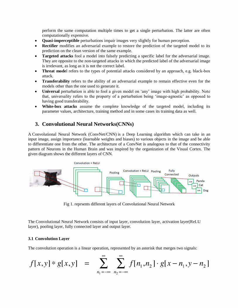
3. Convolutional Neural Networks(CNNs)
A Convolutional Neural Network (ConvNet/CNN) is a Deep Learning algorithm which can take in an input image, assign importance (learnable weights and biases) to various objects in the image and be able
to differentiate one from the other. The architecture of a ConvNet is analogous to that of the connectivity
pattern of Neurons in the Human Brain and was inspired by the organization of the Visual Cortex. The given diagram shows the different layers of CNN.
Fig 1. reprsents different layers of Convolutional Neural Network
The Convolutional Neural Network consists of input layer, convolution layer, activation layer(ReLU layer), pooling layer, fully connected layer and output layer.
3.1 Convolution Layer
The convolution operation is a linear operation, represented by an asterisk that merges two signals:

Two-dimensional convolutions are used in image processing to implement image filters, for example, to find a specific patch on an image or to find some feature in an image. The main hyper parameters that
control the behavior of the convolution layer are as follows:
Kernel size (K): How big your sliding windows are in pixels. Small is generally better
and usually odd value such as 1, 3, 5 or sometimes rarely 7 are used.
Stride (S): How many pixels the kernel window will slide at each step of convolution.
This is usually set to 1, so no locations are missed in an image but can be higher if we want to reduce the input size down at the same time.
Zero padding (pad): The amount of zeros to put on the image border. Using padding
allows the kernel to completely filter every location of an input image, including the edges.
Number of filters (F): How many filters our convolution layer will have. It controls the
number of patterns or features that a convolution layer will look for.
3.2 ReLu Layer
ReLU or Rectified Linear Unit simply changes all the negative values to 0 while leaving the positives values unchanged.
F (x) = max (0, x)
3.3 Pooling Layer
The pooling layer is used to reduce the spatial dimensions of our activation layer, but not volume depth,
in a CNN. They are non parametric way of doing this, meaning that the pooling layer has no weights in it. Basically, the following is what you gain from using pooling layer:
Cheap way of summarizing spatially related information in an input.
By having less spatial information, you gain computation performance.
You get some translation invariance in your network.
3.4 Fully Connected Layer
Fully Connected simply means all nodes in one layer are connected to the outputs of the next layer. The
FC Layer outputs the class probabilities, where each class is assigned a probability. All probabilities must sum to 1, e,g (0.2, 0.5, 0.3).
3.5 Output Layer (Softmax Layer)
The activation function used to produce these probabilities is the Soft Max Function as it turns the outputs of the FC layer (last layer) into probabilities. For example, Let say the output of the last FC
layer was [2, 1, 1]. Applying the softmax ‘squashes’ these real value numbers into probabilities that sum to one: the output would therefore be: [0.7, 0.2, 0.1] .
4 Datasets
The datasets which are used to create adversarial images in this research paper are given below.

4.1 MNIST
The MNIST (“NIST” stands for National Institute of Standards and Technology while the “M” stands for
“modified” as the data has been preprocessed to reduce any burden on computer vision processing and
focus solely on the task of digit recognition) dataset is one of the most well studied datasets in the computer vision and machine learning literature. The goal of this dataset is to correctly classify the
handwritten digits 0 to 9. In many cases, this dataset is a benchmark, a standard to which machine
learning algorithms are ranked. MNIST itself consists of 60,000 training images and 10,000 testing images. Each feature vector is 784-dim, corresponding to the (28 x 28) grayscale pixel intensities of the
image. These grayscale pixel intensities are unsigned integers, falling into the range [0, 255].
4.2 Fashion-MNIST
MNIST comprises 70,000 grayscale images of 28 x 28 pixels resolution. Each image depicts an item of
clothing that can be separated into one of 10 classifications: T-shirt/top, Trouser, Pullover, Dress, Coat, Sandal, Shirt, Sneaker, Bag, or Ankle boot.
4.3 CIFAR-10
Just like MNIST, CIFAR-10 is considered another standard benchmark dataset for image classification in
the computer vision and machine learning literature. CIFAR-10 consists of 60,000 32x32x3 (RGB)
images resulting in a feature vector dimensionality of 3072. As the name suggests, CIFAR-10 consists of
10 classes, including: airplanes, automobiles, birds, cats, deer, dogs, frogs, horses, ships, and trucks.
4.4 CALTECH-101
The dataset of 8,677 images includes 101 categories spanning a diverse range of objects, including
elephants, bicycles, soccer balls, and even human brains, just to name a few. The CALTECH-101 dataset
exhibits heavy class imbalances (meaning that there are more example images for some categories than
others), making it interesting to study from a class imbalance perspective.
4.5 FRUIT-360
A high-quality, dataset of images containing fruits and vegetables. The following fruits and vegetables are included: Apples (different varieties: Crimson Snow, Golden, Golden-Red, Granny Smith, Pink Lady, Red, Red Delicious), Apricot, Avocado, Avocado ripe, Banana (Yellow, Red, Lady Finger).
5 Training CNNs on the above Datasets
In this section, we will train CNNs model on the above mentioned datasets and present the results of the
training and testing set of above datasets. We followed CNN LeNet-5 architecture for MNIST and
FASHION-MNIST datasets and followed CNN VGG16 architecture for CIFAR-10, CALTECH-101, FRUIT-360 but we can use (VGG-3) three layer blocks of VGG16 for CIAR-10, (VGG-5) five layer
blocks of VGG16 for CALTECH-101, FRUIT-360 due to the small dimension of images in these datasets. The results of our experiments are given in the table below.

Table 1. Results of experiments CNN Models on the above datasets
Datasets CNNs Model Architecture Training Accuracy Training Loss
Testing Accuracy Testing Loss
MNIST LeNet-5 99.88 % 0.0043 98.83 % 0.0499
FASHION-MNIST LeNet-5 97.89% 0.0578 91.54 % 0.3251
CIFAR-10 VGG-3 98.16% 0.0537 79.89 % 0.9347
CALTECH-101 VGG-5 96.77% 0.1126 93.23 % 0.2215
FRUIT-360 VGG-5 99.72 % 0.0134 100 % 0.0001
Fig 2. Predictions of some test images from MNIST dataset. Predicted classes are enclosed in square brackets.
Fig3. Predictions of some test images from FASHION-MNIST dataset. Predicted classes are enclosed in square brackets.
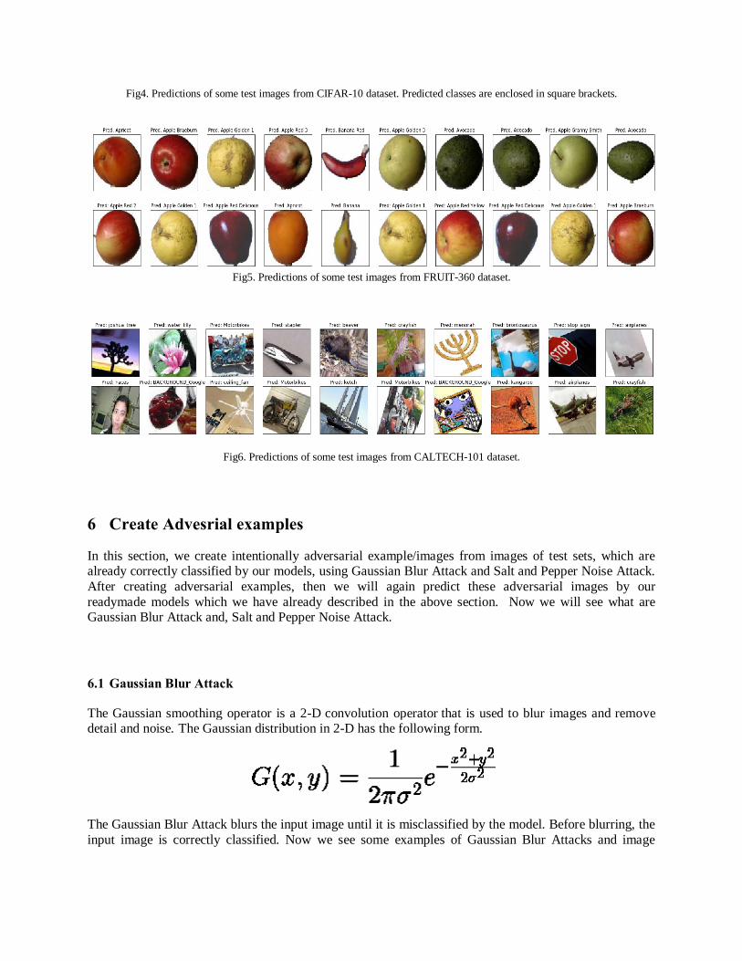
Fig4. Predictions of some test images from CIFAR-10 dataset. Predicted classes are enclosed in square brackets.
Fig5. Predictions of some test images from FRUIT-360 dataset.
Fig6. Predictions of some test images from CALTECH-101 dataset.
6 Create Advesrial examples
In this section, we create intentionally adversarial example/images from images of test sets, which are already correctly classified by our models, using Gaussian Blur Attack and Salt and Pepper Noise Attack.
After creating adversarial examples, then we will again predict these adversarial images by our
readymade models which we have already described in the above section. Now we will see what are Gaussian Blur Attack and, Salt and Pepper Noise Attack.
6.1 Gaussian Blur Attack
The Gaussian smoothing operator is a 2-D convolution operator that is used to blur images and remove detail and noise. The Gaussian distribution in 2-D has the following form.
The Gaussian Blur Attack blurs the input image until it is misclassified by the model. Before blurring, the
input image is correctly classified. Now we see some examples of Gaussian Blur Attacks and image
misclassification on our five selected datasets MNIST, FASHION-MNIST, CIFAR-10, CALTECH-101 and FRUIT-360, which are given below.
(a) (b) (c) (d)
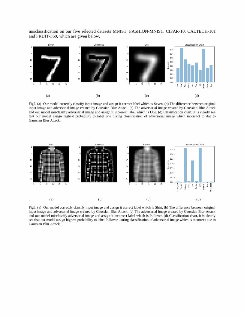
Fig7. (a) Our model correctly classify input image and assign it correct label which is Seven. (b) The difference between original input image and adversarial image created by Gaussian Blur Attack. (c) The adversarial image created by Gaussian Blur Attack
and our model misclassify adversarial image and assign it incorrect label which is One. (d) Classification chart, it is clearly see that our model assign highest probability to label one during classification of adversarial image which incorrect to due to Gaussian Blur Attack.
. (a) (b) (c) (d)
Fig8. (a) Our model correctly classify input image and assign it correct label which is Shirt. (b) The difference between original input image and adversarial image created by Gaussian Blur Attack. (c) The adversarial image created by Gaussian Blur Attack and our model misclassify adversarial image and assign it incorrect label which is Pullover. (d) Classification chart, it is clearly see that our model assign highest probability to label Pullover, during classification of adversarial image which is incorrect due to Gaussian Blur Attack.
. (a) (b) (c) (d)
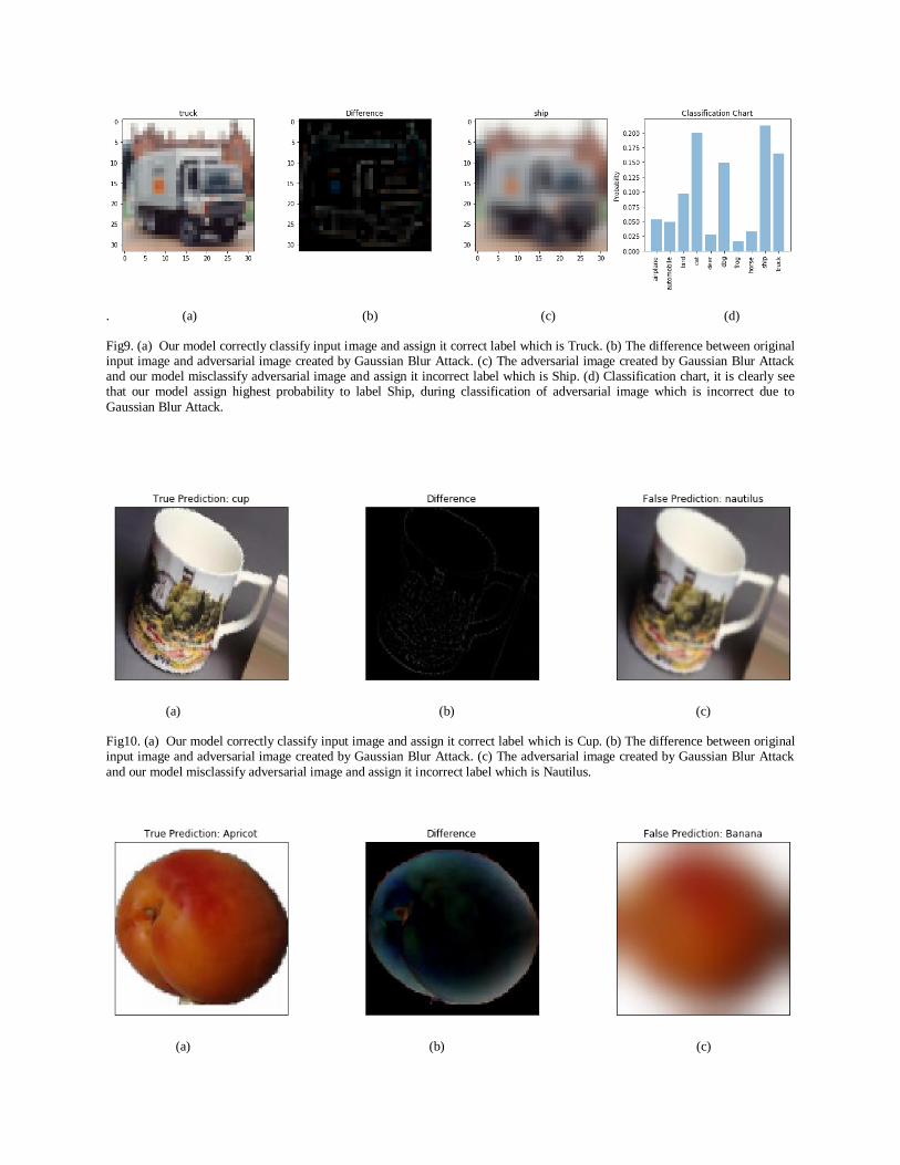
Fig9. (a) Our model correctly classify input image and assign it correct label which is Truck. (b) The difference between original input image and adversarial image created by Gaussian Blur Attack. (c) The adversarial image created by Gaussian Blur Attack and our model misclassify adversarial image and assign it incorrect label which is Ship. (d) Classification chart, it is clearly see that our model assign highest probability to label Ship, during classification of adversarial image which is incorrect due to
Gaussian Blur Attack.
(a) (b) (c)
Fig10. (a) Our model correctly classify input image and assign it correct label which is Cup. (b) The difference between original input image and adversarial image created by Gaussian Blur Attack. (c) The adversarial image created by Gaussian Blur Attack
and our model misclassify adversarial image and assign it incorrect label which is Nautilus.
(a) (b) (c)
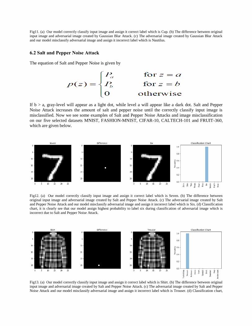
Fig11. (a) Our model correctly classify input image and assign it correct label which is Cup. (b) The difference between original input image and adversarial image created by Gaussian Blur Attack. (c) The adversarial image created by Gaussian Blur Attack and our model misclassify adversarial image and assign it incorrect label which is Nautilus.
6.2 Salt and Pepper Noise Attack
The equation of Salt and Pepper Noise is given by
If b > a, gray-level will appear as a light dot, while level a will appear like a dark dot. Salt and Pepper
Noise Attack increases the amount of salt and pepper noise until the correctly classify input image is
misclassified. Now we see some examples of Salt and Pepper Noise Attacks and image misclassification
on our five selected datasets MNIST, FASHION-MNIST, CIFAR-10, CALTECH-101 and FRUIT-360, which are given below.
Fig12. (a) Our model correctly classify input image and assign it correct label which is Seven. (b) The difference between original input image and adversarial image created by Salt and Pepper Noise Attack. (c) The adversarial image created by Salt and Pepper Noise Attack and our model misclassify adversarial image and assign it incorrect label which is Six. (d) Classification chart, it is clearly see that our model assign highest probability to label six during classification of adversarial image which is incorrect due to Salt and Pepper Noise Attack.
Fig13. (a) Our model correctly classify input image and assign it correct label which is Shirt. (b) The difference between original input image and adversarial image created by Salt and Pepper Noise Attack. (c) The adversarial image created by Salt and Pepper Noise Attack and our model misclassify adversarial image and assign it incorrect label which is Trouser. (d) Classification chart,

it is clearly see that our model assign highest probability to label trouser during classification of adversarial image which is incorrect due to Salt and Pepper Noise Attack.
Fig14. (a) Our model correctly classify input image and assign it correct label which is Truck. (b) The difference between original input image and adversarial image created by Salt and Pepper Noise Attack. (c) The adversarial image created by Salt and Pepper Noise Attack and our model misclassify adversarial image and assign it incorrect label which is Horse. (d)
Classification chart, it is clearly see that our model assign highest probability to label horse during classification of adversarial image which is incorrect due to Salt and Pepper Noise Attack.
Fig15. (a) Our model correctly classify input image and assign it correct label which is Cup. (b) The difference between original input image and adversarial image created by Salt and Pepper Noise Attack. (c) The adversarial image created by Salt and Pepper Noise Attack and our model misclassify adversarial image and assign it incorrect label which is Panda.
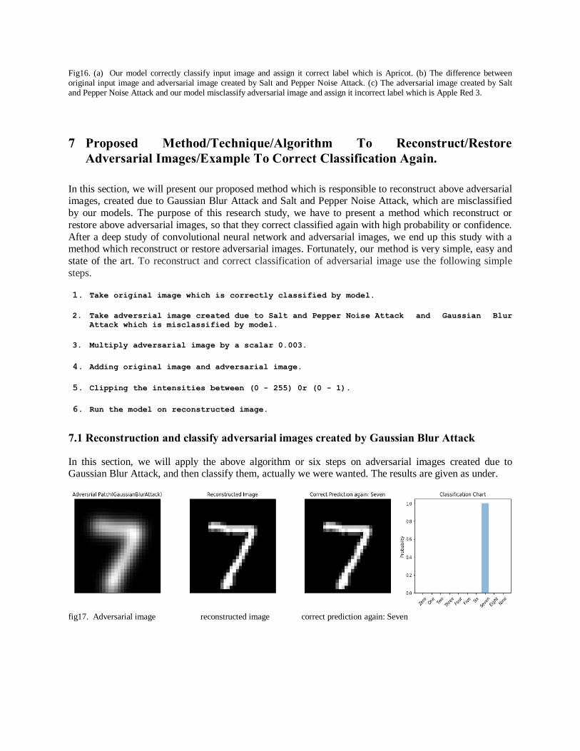
Fig16. (a) Our model correctly classify input image and assign it correct label which is Apricot. (b) The difference between original input image and adversarial image created by Salt and Pepper Noise Attack. (c) The adversarial image created by Salt and Pepper Noise Attack and our model misclassify adversarial image and assign it incorrect label which is Apple Red 3.
7 Proposed Method/Technique/Algorithm To Reconstruct/Restore
Adversarial Images/Example To Correct Classification Again.
In this section, we will present our proposed method which is responsible to reconstruct above adversarial images, created due to Gaussian Blur Attack and Salt and Pepper Noise Attack, which are misclassified
by our models. The purpose of this research study, we have to present a method which reconstruct or
restore above adversarial images, so that they correct classified again with high probability or confidence.
After a deep study of convolutional neural network and adversarial images, we end up this study with a method which reconstruct or restore adversarial images. Fortunately, our method is very simple, easy and
state of the art. To reconstruct and correct classification of adversarial image use the following simple
steps.
1. Take original image which is correctly classified by model.
2. Take adversrial image created due to Salt and Pepper Noise Attack and Gaussian Blur
Attack which is misclassified by model.
3. Multiply adversarial image by a scalar 0.003.
4. Adding original image and adversarial image.
5. Clipping the intensities between (0 - 255) 0r (0 - 1).
6. Run the model on reconstructed image.
7.1 Reconstruction and classify adversarial images created by Gaussian Blur Attack
In this section, we will apply the above algorithm or six steps on adversarial images created due to Gaussian Blur Attack, and then classify them, actually we were wanted. The results are given as under.
fig17. Adversarial image reconstructed image correct prediction again: Seven

Fig18. (a) Adversarial image created due to Gaussian Blur Attack. (b) Reconstructed adversarial image by applying our proposed method. (c) Our model predict correct label shirt of reconstructed adversarial image again. (d) Classification chart, it is clearly see that our model assign highest probability to label shirt during classification of reconstructed adversarial image which is correct.
Fig19. (a) Adversarial image created due to Gaussian Blur Attack. (b) Reconstructed adversarial image by applying our proposed
method. (c) Our model predicts correct label truck of reconstructed adversarial image again. (d) Classification chart, it is clearly see that our model assign highest probability to label truck during classification of reconstructed adversarial image which is correct.
Fig20. (a) Adversarial image created due to Gaussian Blur Attack. (b) Reconstructed adversarial image by applying our proposed method. (c) Our model predicts correct label cup of reconstructed adversarial image again.
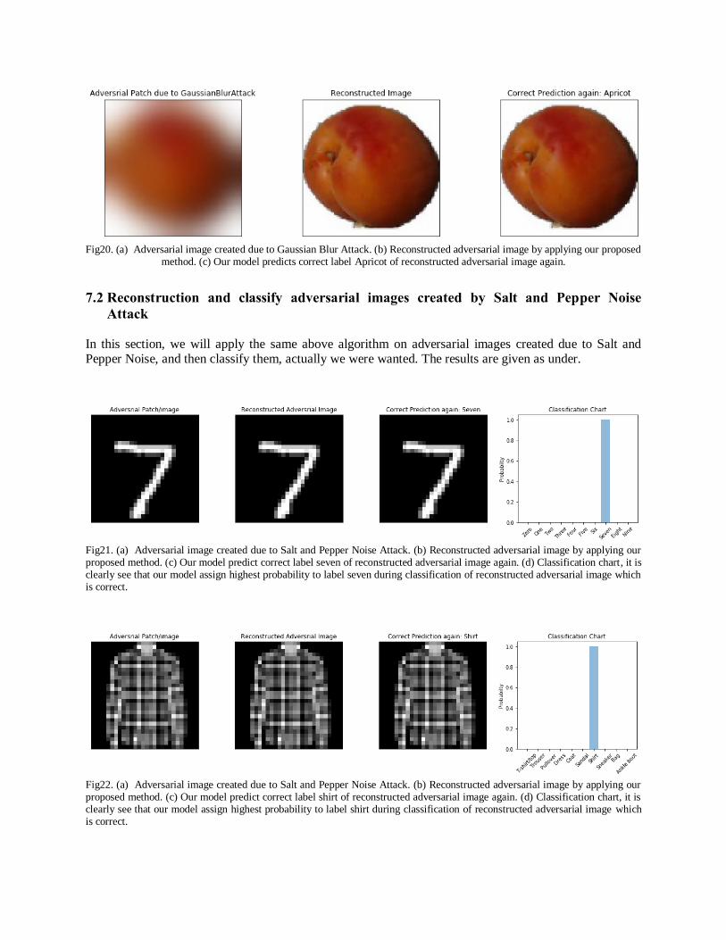
Fig20. (a) Adversarial image created due to Gaussian Blur Attack. (b) Reconstructed adversarial image by applying our proposed
method. (c) Our model predicts correct label Apricot of reconstructed adversarial image again.
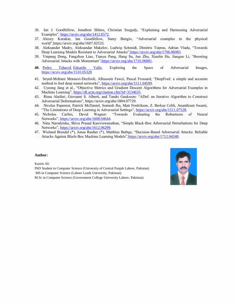
7.2 Reconstruction and classify adversarial images created by Salt and Pepper Noise
Attack
In this section, we will apply the same above algorithm on adversarial images created due to Salt and Pepper Noise, and then classify them, actually we were wanted. The results are given as under.
Fig21. (a) Adversarial image created due to Salt and Pepper Noise Attack. (b) Reconstructed adversarial image by applying our proposed method. (c) Our model predict correct label seven of reconstructed adversarial image again. (d) Classification chart, it is clearly see that our model assign highest probability to label seven during classification of reconstructed adversarial image which is correct.
Fig22. (a) Adversarial image created due to Salt and Pepper Noise Attack. (b) Reconstructed adversarial image by applying our proposed method. (c) Our model predict correct label shirt of reconstructed adversarial image again. (d) Classification chart, it is clearly see that our model assign highest probability to label shirt during classification of reconstructed adversarial image which is correct.

Fig23. (a) Adversarial image created due to Salt and Pepper Noise Attack. (b) Reconstructed adversarial image by applying our proposed method. (c) Our model predicts correct label truck of reconstructed adversarial image again. (d) Classification chart, it is clearly see that our model assign highest probability to label truck during classification of reconstructed adversarial image which is correct.
Fig24. (a) Adversarial image created due to Salt and Pepper Noise Attack. (b) Reconstructed adversarial image by applying our proposed method. (c) Our model predict correct label cup of reconstructed adversarial image again.
Fig24. (a) Adversarial image created due to Salt and Pepper Noise Attack. (b) Reconstructed adversarial image by applying our proposed method. (c) Our model predict correct label Apricot of reconstructed adversarial image again.
8 Conclusion
In this paper, our main purpose is to propose a method which will reconstruct the adversarial images in such a way that these reconstructed adversarial images are correctly classified again by our CNN models.
Therefore, first we have created adversarial images by using two adversarial attacks which are Gaussian

Blur Attack and, Salt and Pepper Noise Attack. These adversarial images are misclassified by our trained CNN models. Then we proposed a method which reconstructs adversarial images. After reconstruction of
adversarial images, our trained CNN models are correctly classified these adversarial images. Hence we
have proved in this study, we can reconstruct adversarial images in a way such that they are correctly classified by a CNN model again.
9 Future Work
In future, we want to continue, to work on adversarial images for the sake of security and robustness of
Convolutional Neural Networks. There are so many adversarial attacks have developed which is a serious
threat to fool a trained convolutional neural network. Therefore, it is much needed now, to concentrate on the robustness and security of neural network.
References
1. Krizhevsky, I. Sutskever and G. E. Hinton, Imagenet classification with deep convolutional neural
networks. In Advances in neural information processing systems, pp. 1097-1105, 2012.
2. Y. LeCun, B. Boser, J. S. Denker, D. Henderson, R. E. Howard, W. Hubbard and L. D. Jackel,
Backpropagation applied to handwritten zip code recognition. Neural computation, vol. 1m no. 4, pp. 541-
551, 1989.
3. J. Deng, W. Dong, R. Socher, L. J. Li, K. Li, and L. Fei-Fei, Imagenet: A large-scale hierarchical image database. In IEEE Conference on Computer Vision and Pattern Recognition, pp. 248-255, 2009.
4. Esteva, B. Kuprel, R. A. Novoa, J. Ko, S. M. Swetter, H. M. Blau, S. Thrun, Dermatologist-level
classification of skin cancer with deep neural networks, Nature, vol. 542, pp. 115 - 118, 2017.
5. Objects Detection Machine Learning TensorFlow Demo,
https://play.google.com/store/apps/details?id=org.tensorflow.
detect&hl=en, Accessed December 2019.
6. D. Silver, J. Schrittwieser, K. Simonyan, I. Antonoglou, A. Huang, A. Guez, Y. Chen, Mastering the game of go without human knowledge. Nature, vol. 550, no. 7676, pp. 354-359, 2017.
7. K. He, X. Zhang, S. Ren, and J. Sun, Deep residual learning for image recognition, In Proceedings of the
IEEE conference on computer vision and pattern recognition, pp. 770-778, 2016.
8. C. Szegedy, V. Vincent, S. Ioffe, J. Shlens, and Z.Wojna. Rethinking the inception architecture for
computer vision, In Proceedings of the IEEE Conference on Computer Vision and Pattern Recognition,
pp.2818-282, 2016.
9. G. Huang, Z. Liu, K. Q. Weinberger, and L. Maaten, Densely connected convolutional networks, arXiv
preprint arXiv:1608.06993, 2016.
10. Vedaldi and K. Lenc, MatConvNet – Convolutional Neural Networks for MATLAB, In Proceeding of the
ACM International Conference on Multimedia, 2015.
11. J. Yangqing, E. Shelhamer, J. Donahue, S. Karayev, J. Long, R. Girshick, S. Guadarrama, T. Darrell,
Caffe: Convolutional Architecture for Fast Feature Embedding, arXiv preprint arXiv:1408.5093, 2014. 12. M. Abadi, A. Agarwal, P. Barham, E. Brevdo, Z. Chen, C. Citro, G. S. Corrado, A. Davis, J. Dean, M.
Devin, S. Ghemawat, I. Goodfellow, A. Harp, G. Irving, M. Isard, R. Jozefowicz, Y. Jia, L. Kaiser, M.
Kudlur, J. Levenberg, D. Mane, M Schuster, R. Monga, S. Moore, D. Murray, C. Olah, J. Shlens, B.
Steiner, I. Sutskever, K. Talwar, P. Tucker, V. Vanhoucke, V. Vasudevan, F. Viegas, O. Vinyals, P.
Warden, M.Wattenberg, M.Wicke, Y. Yu, and X. Zheng, TensorFlow: Large-scale machine learning on
heterogeneous systems, 2015. Software available from tensorflow.org.
13. E. Ackerman, How Drive.ai is mastering autonomous driving with deep learning, https://spectrum.
ieee.org/cars-that-think/transportation/self-driving/how-driveai-is-mastering-autonomous-driving-with-
deep-learning,Accessed December 2019.
14. M. M. Najafabadi, F. Villanustre, T. M. Khoshgoftaar, N. Seliya, R. Wald and E. Muharemagic, Deep
learning applications and challenges in big data analytics, Journal of Big Data, vol. 2, no. 1, 2015.

15. N. Papernot, P. McDaniel, A. Sinha, M. Wellman, Towards the Science of Security and Privacy in Machine
Learning, arXiv preprint arXiv:1611.03814, 2016.
16. K. Grosse, N. Papernot, P. Manoharan, M. Backes, and P. Mc-Daniel, Adversarial examples for malware
detection, In European Symposium on Research in Computer Security, pp. 62-79. 2017.
17. M. Volodymyr, K. Kavukcuoglu, D. Silver, A. A. Rusu, J. Veness, M. G. Bellemare, A. Graves, M. Riedmiller, A. K. Fidjeland, G. Ostrovski, Human-level control through deep reinforcement learning,
Nature, vol. 518, no. 7540, pp. 529-533, 2015.
18. A. Giusti, J. Guzzi, D. C. Ciresan, F. He, J. P. Rodriguez, F. Fontana, M. Faessler, A machine learning
approach to visual perception of forest trails for mobile robots, IEEE Robotics and Automation Letters, vol.
1, no. 2, pp. 661 - 667, 2016.
19. G. Hinton, L. Deng, D. Yu, G. E. Dahl, A. R. Mohamed, N. Jaitly, and B. Kingsbury, Deep neural networks
for acoustic modeling in speech recognition: The shared views of four research groups, IEEE Signal
Processing Magazine, vol. 29, no. 6, pp. 82-97, 2012.
20. C. Middlehurst, China unveils world’s first facial recognition ATM,
http://www.telegraph.co.uk/news/worldnews/asia/china/11643314/China-unveils-worlds-first-facial-
recognition-ATM.html, 2015.
21. Ian J. Goodfellow, Jonathon Shlens, and Christian Szegedy. Explaining and harnessing adversarial examples. arXiv preprint arXiv:1412.6572, 2014.
22. Anh Mai Nguyen, Jason Yosinski, and Jeff Clune. Deep neural networks are easily fooled: High confidence
predictions for unrecognizable images. In IEEE Conference on Computer Vision and Pattern Recognition,
CVPR 2015, Boston, MA, USA, June 7-12, 2015, pages 427–436. IEEE Computer Society, 2015.
23. Mahmood Sharif, Sruti Bhagavatula, Lujo Bauer, and Michael K. Reiter. Accessorize to a crime: Real and
stealthy attacks on state-of-the-art face recognition. In Edgar R. Weippl, Stefan Katzenbeisser, Christopher
Kruegel, Andrew C. Myers, and Shai Halevi, editors, Proceedings of the 2016 ACM SIGSAC Conference
on Computer and Communications Security, Vienna, Austria, October 24-28, 2016, pages 1528–1540.
ACM, 2016.
24. Christian Szegedy, Wojciech Zaremba, Ilya Sutskever, Joan Bruna, Dumitru Erhan, Ian J. Goodfellow, and Rob Fergus. Intriguing properties of neural networks. arXiv preprint arXiv:1312.6199, 2013.
25. Alhussein Fawzi, Omar Fawzi, and Pascal Frossard. Analysis of classifiers’ robustness to adversarial
perturbations. arXiv preprint arXiv:1502.02590, 2015.
26. Alexey Kurakin, Ian J. Goodfellow, and Samy Bengio. Adversarial machine learning at scale. arXiv
preprint arXiv:1611.01236, 2016.
27. Nicolas Papernot and Patrick D. McDaniel. On the effectiveness of defensive distillation. arXiv preprint
arXiv:1607.05113, 2016.
28. Andras Rozsa, Manuel Günther, and Terrance E. Boult. Towards robust deep neural networks with BANG.
arXiv preprint arXiv:1612.00138, 2016.
29. MohamadAli Torkamani. Robust Large Margin Approaches for Machine Learning in Adversarial Settings.
PhD thesis, University of Oregon, 2016.
30. Jure Sokolic, Raja Giryes, Guillermo Sapiro, and Miguel RD Rodrigues. Robust large margin deep neural networks. arXiv preprint arXiv:1605.08254, 2016.
31. Florian Tramèr, Nicolas Papernot, Ian J. Goodfellow, Dan Boneh, and Patrick D. McDaniel. The space of
transferable adversarial examples. arXiv preprint arXiv:1704.03453, 2017.
32. Anh Mai Nguyen, Jason Yosinski, and Jeff Clune. Deep neural networks are easily fooled: High confidence
predictions for unrecognizable images. In IEEE Conference on Computer Vision and Pattern Recognition,
CVPR 2015, Boston, MA, USA, June 7-12, 2015, pages 427–436. IEEE Computer Society, 2015.
33. Mahmood Sharif, Sruti Bhagavatula, Lujo Bauer, and Michael K. Reiter. Accessorize to a crime: Real and
stealthy attacks on state-of-the-art face recognition. In Edgar R. Weippl, Stefan Katzenbeisser, Christopher
Kruegel, Andrew C. Myers, and Shai Halevi, editors, Proceedings of the 2016 ACM SIGSAC Conference
on Computer and Communications Security, Vienna, Austria, October 24-28, 2016, pages 1528–1540.
ACM, 2016. 34. Seyed-Mohsen Moosavi-Dezfooli, Alhussein Fawzi, and Pascal Frossard. Deepfool: A simple and accurate
method to fool deep neural networks. In 2016 IEEE Conference on Computer Vision and Pattern
Recognition, CVPR 2016, Las Vegas, NV, USA, June 27-30, 2016, pages 2574–2582. IEEE Computer
Society, 2016.
35. Intriguing properties of neural networks. https://arxiv.org/pdf/1312.6199.pdf
36. Ian J. Goodfellow, Jonathon Shlens, Christian Szegedy, “Explaining and Harnessing Adversarial
Examples”, https://arxiv.org/abs/1412.6572.
37. Alexey Kurakin, Ian Goodfellow, Samy Bengio, “Adversarial examples in the physical
world”,https://arxiv.org/abs/1607.02533.
38. Aleksander Madry, Aleksandar Makelov, Ludwig Schmidt, Dimitris Tsipras, Adrian Vladu, “Towards Deep Learning Models Resistant to Adversarial Attacks”,https://arxiv.org/abs/1706.06083.
39. Yinpeng Dong, Fangzhou Liao, Tianyu Pang, Hang Su, Jun Zhu, Xiaolin Hu, Jianguo Li, “Boosting
Adversarial Attacks with Momentum”,https://arxiv.org/abs/1710.06081.
40. Pedro Tabacof, Eduardo Valle, Exploring the Space of Adversarial Images,
https://arxiv.org/abs/1510.05328
41. Seyed-Mohsen Moosavi-Dezfooli, Alhussein Fawzi, Pascal Frossard, “DeepFool: a simple and accurate
method to fool deep neural networks”, https://arxiv.org/abs/1511.04599.
42. Uyeong Jang et al., “Objective Metrics and Gradient Descent Algorithms for Adversarial Examples in
Machine Learning”, https://dl.acm.org/citation.cfm?id=3134635.
43. Rima Alaifari, Giovanni S. Alberti, and Tandri Gauksson: “ADef: an Iterative Algorithm to Construct
Adversarial Deformations”, https://arxiv.org/abs/1804.07729.
44. Nicolas Papernot, Patrick McDaniel, Somesh Jha, Matt Fredrikson, Z. Berkay Celik, Ananthram Swami, “The Limitations of Deep Learning in Adversarial Settings”, https://arxiv.org/abs/1511.07528.
45. Nicholas Carlini, David Wagner: “Towards Evaluating the Robustness of Neural
Networks”, https://arxiv.org/abs/1608.04644.
46. Nina Narodytska, Shiva Prasad Kasiviswanathan, “Simple Black-Box Adversarial Perturbations for Deep
Networks”, https://arxiv.org/abs/1612.06299.
47. Wieland Brendel (*), Jonas Rauber (*), Matthias Bethge, “Decision-Based Adversarial Attacks: Reliable
Attacks Against Black-Box Machine Learning Models”,https://arxiv.org/abs/1712.04248.
Author:
Kazim Ali
PhD Student in Computer Science (University of Central Punjab Lahore, Pakistan)
MS in Computer Science (Lahore Leads University, Pakistan)
M.Sc in Computer Science (Government College University Lahore, Pakistan)