Towards Practical Differentially Private ConvexOptimization

Roger IyengarCarnegie Mellon University

Om ThakkarBoston University

Joseph P. NearUniversity of California, Berkeley

Abhradeep ThakurtaUniversity of California, Santa Cruz

Dawn SongUniversity of California, Berkeley

Lun WangPeking University

Abstract—Building useful predictive models often in-volves learning from sensitive data. Training models withdifferential privacy can guarantee the privacy of suchsensitive data. For convex optimization tasks, several dif-ferentially private algorithms are known, but none has yetbeen deployed in practice.

In this work, we make two major contributions towardspractical differentially private convex optimization. First,we present Approximate Minima Perturbation, a novelalgorithm that can leverage any off-the-shelf optimizer.We show that it can be employed without any hyperpa-rameter tuning, thus making it an attractive techniquefor practical deployment. Second, we perform an extensiveempirical evaluation of the state-of-the-art algorithms fordifferentially private convex optimization, on a range ofpublicly available benchmark datasets, and real-worlddatasets obtained through an industrial collaboration. Werelease open-source implementations of all the differentiallyprivate convex optimization algorithms considered, andbenchmarks on as many as nine public datasets, four ofwhich are high-dimensional.

I. INTRODUCTION

Building useful predictive models often involves learn-ing from sensitive data. To preserve the privacy ofsuch sensitive data, many systems first carry out thelearning task over the data, and then release just the final“learned” model. However, as many recent works [1],[2], [3] indicate, a model can leak information aboutthe sensitive data it was trained on, even though thedata might have never been made public. To preventsuch information leakage, differential privacy (DP) [4],[5] has been recently used as a gold standard for per-forming learning tasks over sensitive data. It has alsobeen adopted by large-scale corporations like Google[6], Apple [7], etc. Intuitively, DP prevents an adversaryfrom confidently making any conclusions about whethera sample was used in training a model, even while havingaccess to the model and any external side information.

The authors are ordered alphabetically.

With the recent advancements in machine learning andbig data, private convex optimization has proven to beuseful for large-scale learning over sensitive user datathat has been collected by organizations. The objective ofthis work is to provide insight into practical differentiallyprivate convex optimization, with a specific focus onthe classical technique of objective perturbation [8],[9]. Our main technical contribution is to design anew algorithm for private convex optimization that isamenable to real-world scenarios, and provide privacyand utility guarantees for it. In addition, we conducta broad empirical evaluation of approaches for privateconvex optimization, including our new approach. Ourevaluation is more extensive than prior works [8], [10],[11], [12]; it includes nine public datasets, four ofwhich are high-dimensional. Apart from these, we alsoconsider four real-world use cases, obtained in collabo-ration with Uber Technologies, Inc. We provide adviceand resources for practitioners, including open-sourceimplementations [13] of the algorithms evaluated, andbenchmarks on all the public datasets considered.

A. Objective Perturbation and its Practical Feasibility

We focus our attention on the technique of objectiveperturbation, because prior works [8], [9] as well asour own preliminary empirical results have hinted atits superior performance. The standard technique of ob-jective perturbation [8] consists of a two-stage process:“perturbing” the objective function by adding a randomlinear term, and releasing the minima of the perturbedobjective. It has been shown [8], [9] that releasing sucha minima is sufficient for achieving DP guarantees.

However, objective perturbation provides privacyguarantees only if the output of the mechanism is theexact minima of the perturbed objective. Practical algo-rithms for convex optimization often involve the use offirst-order iterative methods, such as gradient descent or

stochastic gradient descent (SGD) due to their scalability.However, such methods typically offer convergence ratesthat depend on the number of iterations carried out bythe method, so they are not guaranteed to reach theexact minima in finite time. As a result, it is not clear ifobjective perturbation in its current form can be appliedin a practical setting, where one is usually constrainedby resources such as computing power, and reaching theminima might not be feasible.

We address the fundamental question of whether an al-ternative to standard objective perturbation exists whichprovides privacy and utility guarantees when the releasedmodel is not necessarily the minima of the perturbedobjective. In this work, we answer this question in thepositive: it is possible to get privacy and utility guaran-tees even if the system releases a noisy “approximate”minima of the perturbed objective. A major implicationof this result is that one can use first-order iterativemethods in combination with such an approach. This canbe highly beneficial in terms of the time taken to obtaina private solution, as first-order methods often succeedto find a “good” solution very quickly.

B. Our Approach: Approximate Minima Perturbation

We propose Approximate Minima Perturbation(AMP), a strengthened alternative to objectiveperturbation that provides privacy and utility guaranteeswhen the released model is a noisy “approximate”minima for the perturbed objective. We measure theconvergence of a model in terms of the Euclideannorm of the gradient of the perturbed objective at themodel. The scale of the noise added to the approximateminima contains a parameter representing the maximumtolerable gradient norm. This results in a trade-offbetween the gradient norm bound (consequently, theamount of noise to be added to the approximateminima), and the difficulty, in practice, of being ableto obtain an approximate minima within the normbound. This can be useful in settings where a limitedcomputing power is available, which can in turn act asa guide for setting an appropriate norm bound. We notethat if the norm bound is set to zero, then this approachreduces to the setting of standard objective perturbation.Approximate Minima Perturbation also brings with itcertain distinct advantages, which we will describe next.

Approximate Minima Perturbation works for allconvex objective functions: While previous works [8],[9] provide privacy guarantees for objective perturba-tion only when the objective is a loss function of a

generalized linear model1, the guarantees provided forAMP hold for any objective function.2 In both cases,the objective functions are assumed to possess standardproperties like Lipschitz continuity, and smoothness.

Approximate Minima Perturbation is the first fea-sible approach that can leverage any off-the-shelfoptimizer: AMP can accommodate any off-the-shelfoptimizer as a black-box for carrying out its optimizationstep. This enables a simple implementation that inheritsthe scalability properties of the optimizer used, whichcan be particularly important in situations where high-performance optimizers are available. AMP is the onlyknown feasible algorithm for DP convex optimizationthat allows the use of any off-the-shelf optimizer.

Approximate Minima Perturbation has a competitivehyperparameter-free variant: To ensure privacy for analgorithm, its hyperparameters must be chosen eitherindependently of the data, or by using a differentiallyprivate hyperparameter tuning algorithm. Previous work[8], [14], [15] has shown this to be a challenging task.AMP has only four hyperparameters: one related to theLipschitz continuity of the objective, and the other threerelated to splitting the privacy budget within the algo-rithm. In Section V-A, we present a data-independentmethod for setting all of them. Our empirical evalu-ation demonstrates that the resulting hyperparameter-free variant of AMP yields comparable accuracy to thestandard variant with its hyperparameters tuned in a data-dependent manner (which may be non-private).

C. Empirical Evaluation, & Resources for Practitioners

This work also reports on an extensive and broad em-pirical study of the state-of-the-art differentially privateconvex optimization techniques. In addition to AMP andits hyperparameter-free variant, we evaluate four exist-ing algorithms: private gradient descent with minibatch-ing [16], [15], both the variants (convex, and stronglyconvex) of the private Permutation-based SGD algo-rithm [12], and the private Frank-Wolfe algorithm [17].

Our evaluation is the largest to date, including atotal of 13 datasets. We include datasets with a varietyof different properties, including four high-dimensionaldatasets and four real-world use cases represented bydatasets obtained in collaboration with Uber.

The results of our empirical evaluation demonstratethree key findings. First, we confirm the expectation thatthe cost of privacy decreases as dataset size increases.

1The loss function of a generalized linear model is parameterizedby an inner product of the feature vector of the data, and the model.

2Our analysis, in particular, extends to objective perturbation as well.

For all the real-world use cases in our evaluation, weobtain differentially private models that achieve an ac-curacy within 4% of the non-private baseline even forvery conservative settings of the privacy parameters. Forreasonable values of the privacy parameters, the accuracyof the best private model is within 2% of the baseline fortwo of these datasets, essentially identical to the baselinefor one of them, and even slightly higher than thebaseline for one of the datasets! This provides empiricalevidence to further the claims of previous works [18],[19] that DP can also act as a type of regularization,reducing the generalization error.

Second, our results demonstrate a general ordering ofalgorithms in terms of empirical accuracy. Our resultsshow that AMP generally outperforms all the other algo-rithms across all the considered datasets. Under specificconditions like high-dimensionality of the dataset andsparsity of the optimal predictive model for it, we seethat private Frank-Wolfe provides the best performance.

Third, our results show that a hyperparameter-freevariant of AMP achieves nearly the same accuracy as thestandard variant with its hyperparameters tuned in a data-dependent manner. Approximate Minima Perturbation istherefore simple to deploy in practice as it can leverageany off-the-shelf optimizer, and it has a competitivevariant that does not require any hyperparameter tuning.

We provide an open-source implementation [13] ofthe algorithms evaluated, including our ApproximateMinima Perturbation, and a complete set of benchmarksused in producing our empirical results. In addition toenabling the reproduction of our results, this set ofbenchmarks will provide a standard point of referencefor evaluating private algorithms proposed in the future.Our open-source release represents the first benchmarkfor differentially private convex optimization.

D. Main Contributions

The main contributions of this work are as follows:

• We propose Approximate Minima Perturbation, astrengthened alternative to objective perturbation thatprovides privacy guarantees even for an approximateminima of the perturbed objective, and thereforeallows the use of any off-the-shelf optimizer. Noprevious approach provides this capability. Comparedto previous approaches, AMP also provides improvedutility in practice, and works with any convex lossfunction under standard assumptions.

• We conduct the largest empirical study to date ofstate-of-the-art DP convex optimization approaches,including as many as nine public datasets, four of

which are high-dimensional. Our results demonstratethat AMP generally provides the best accuracy.

• We evaluate DP convex optimization on four real-world use cases, obtained in collaboration with Uber.Our results suggest that for the large-scale datasetsused in practice, privacy-preserving models can obtainessentially the same accuracy as non-private modelsfor reasonable values of the privacy parameters. Inone case, we show that a DP model achieves a higheraccuracy than the non-private baseline.

• We present a competitive hyperparameter-free variantof AMP, allowing the approach to be deployed with-out the need for tuning on publicly available datasets,or by a DP hyperparameter tuning algorithm.

• We release open-source implementations [13] of allthe algorithms we evaluate, and the first benchmarksfor differentially private convex optimization algo-rithms on as many as nine public datasets.

II. RELATED WORK

Convex optimization in the non-private setting has along history, with several excellent resources providinga good overview [20], [21]. A lot of recent advanceshave been made in the field of convex Empirical RiskMinimization (ERM) as well. A comprehensive list ofworks on stochastic convex ERM has been provided in[22], whereas [23] provides dimension-dependent lowerbounds for the sample complexity required for stochasticconvex ERM and uniform convergence.

A large body of existing work examines the problemof differentially private convex ERM. The techniquesof output perturbation and objective perturbation werefirst proposed in [8]. Near dimension-independent riskbounds for both the techniques were provided in [11];however, the bounds are achieved for the standard set-tings of the techniques, which provide privacy guaran-tees only for the minima of their respective objectivefunctions. A private SGD algorithm was first given in[10], and optimal risk bounds were provided for a laterversion of private SGD in [16]. A variant of outputperturbation was proposed in [12] that requires the useof permutation-based SGD, and reduces sensitivity usingproperties of that algorithm. Several works [9], [24] dealwith DP convex ERM in the setting of high-dimensionalsparse regression, but the algorithms in these worksalso require obtaining the minima. The Frank-Wolfealgorithm [25] has also seen a resurgence lately [26],[27], [28], [29]. We study the performance of a DPversion of Frank-Wolfe [17] in our empirical analysis.

There are also works in DP convex optimization apartfrom the ERM model. Many recent works [30], [31], [32]examine the setting of online learning, whereas high-dimensional kernel learning is considered in [33]; thesesettings are quite different from ours, and the results areincomparable. There have also been works [34], [35] onDP regression analysis, a subset of DP convex optimiza-tion. However, the privacy guarantees in these hold onlyif the algorithms are able to find some minima. Therehave also been advances in DP non-convex optimization,including deep learning [36], [15]. A broad survey ofworks in DP machine learning has been provided in [37].

Previous empirical evaluations have provided limitedinsight into the practical performance of the various algo-rithms for DP convex optimization. Output perturbationand objective perturbation are evaluated on two datasetsin [8] and [11], and private SGD is evaluated in [10]. Wuet al. [12] perform the broadest comparison, includingtheir own approach, and two variants of private SGD[10], [16] on six datasets, but they do not include objec-tive perturbation. No prior evaluation considers the state-of-the-art algorithms from all three major lines of workin the area (output perturbation, objective perturbation,and private SGD). Moreover, none of the prior evalua-tions considers high-dimensional data—a maximum of75 dimensions is considered in [12].

Our empirical evaluation is the most complete to date.We evaluate state-of-the-art algorithms from all 3 linesof work on 9 public datasets and 4 real-world use cases.We consider low-dimensional and high-dimensional (asmany as 47,236 dimensions) datasets. In addition, werelease open-source implementations for all algorithms,and benchmarking scripts to reproduce our results [13].

III. PRELIMINARIES

In this section, we formally define the notation, im-portant definitions, and results used in this work.

Given an n-element dataset D = {d1, d2, . . . , dn}, s.t.di ∈ D for i ∈ [n], the objective is to get a model θ fromthe following unconstrained optimization problem:

θ ∈ arg minθ∈Rp

L(θ;D),

where L(θ;D) = 1n

n∑i=1

`(θ; di) is the empirical risk,

p > 0, and `(θ; di) is defined as a loss function for di thatis convex in the first parameter θ ∈ Rp. This formulationfalls under the framework of ERM, which is useful invarious settings, including the widely applicable problemof classification in machine learning via linear regres-sion, logistic regression, or support vector machines. The

notation ‖x‖ is used to represent the L2-norm of a vectorx. Next, we define certain basic properties of functionsthat will be helpful in further sections.

Definition III.1. A function f : Rp → R :

• is a convex function if for all θ1, θ2 ∈ Rp,f(θ1)− f(θ2) ≥ 〈∇f(θ2), θ1 − θ2〉.

• is a ξ-strongly convex function if for all θ1, θ2 ∈ Rp,f(θ1) ≥ f(θ2) + 〈∇f(θ2), θ1 − θ2〉+ ξ

2‖θ1 − θ2‖2,or equivalently,〈∇f(θ1)−∇f(θ2), (θ1 − θ2)〉 ≥ ξ‖θ1 − θ2‖2.

• has Lq-Lipschitz constant L if for all θ1, θ2 ∈ Rp,|f(θ1)− f(θ2)| ≤ L · ‖θ1 − θ2‖q .

• is β-smooth if for all θ1, θ2 ∈ Rp,‖∇f(θ1)−∇f(θ2)‖ ≤ β · ‖θ1 − θ2‖.

To establish the notion of DP, we first define neigh-boring datasets. We will refer to a pair of datasetsD,D′ ∈ Dn as neighbors, if D′ can be obtained fromD by modifying one sample di ∈ D for some i ∈ [n].

Definition III.2 ((ε, δ)-Differential Privacy [4], [5]). A(randomized) algorithm M with input domain Dn andoutput range R is (ε, δ)-differentially private if for allpairs of neighboring inputs D,D′ ∈ Dn, and everymeasurable S ⊆ R, we have with probability over thecoin flips of M that:

Pr (M(D) ∈ S) ≤ eε · Pr (M(D′) ∈ S) + δ.

One of the most common techniques for achieving dif-ferential privacy is the Gaussian mechanism, for whichwe first need the L2-sensitivity of a function.

Definition III.3 (L2-sensitivity). A function f : Dn →Rp has L2-sensitivity ∆ if

maxD,D′∈Dn s.t.

(D,D′) neighbors

‖f(D)− f(D′)‖ = ∆.

Lemma III.1 (Gaussian mechanism [38]). If a functionf : Dn → Rp has L2-sensitivity ∆, then the mechanismM , which on input D ∈ Dn outputs f(D) + b, whereb ∼ N (0, σ2Ip×p) and σ = ∆

ε

(1 +

√2 log 1

δ

), satisfies

(ε, δ)-differential privacy. Here, N(0, σ2Ip×p) denotesthe p-dimensional zero-mean Gaussian distribution witheach dimension having variance σ2.

Lastly, we define Generalized Linear Models (GLMs).

Definition III.4 (Generalized Linear Model). For amodel space θ ∈ Rp, where p > 0, the sample spaceD in a GLM is defined as the cartesian product of ap-dimensional feature space X ⊆ Rp and a label spaceY , i.e., D = X × Y . Thus, each data sample di ∈ D

can be decomposed into a feature vector xi ∈ X , and alabel yi ∈ Y . Moreover, the loss function `(θ; di) for aGLM is a function of xTi θ and yi.

IV. APPROXIMATE MINIMA PERTURBATION

In this section, we will describe Approximate MinimaPerturbation, a strengthened alternative to objective per-turbation that provides DP guarantees in the case evenwhen the output of the algorithm is not the actual minimaof the perturbed objective function. The perturbed objec-tive takes the form L(θ;D)+ Λ

2 ‖θ‖2+〈b, θ〉, where b is a

random variable drawn from an appropriate distribution,and Λ is an appropriately chosen regularization constant.We make two crucial improvements over the originalobjective perturbation algorithm [8], [9]:• The privacy guarantee of objective perturbation holds

only at the exact minima of the underlying optimiza-tion problem, which is never guaranteed in practicegiven finite time. We show that AMP provides aprivacy guarantee even for an approximate solution.

• Earlier privacy analyses for objective perturbation [8],[9] hold only when the loss function `(θ; d) is a lossfor a GLM (see Definition III.4), as they implicitlymake a rank-one assumption on the Hessian of theloss 52`(θ; d). Via a careful perturbation analysis ofthe Hessian, we extend the analysis to any convex lossfunction under standard assumptions. It is importantto note that AMP reduces to objective perturbation ifthe “approximate” minima condition is tightened togetting the actual minima of the perturbed objective.

Algorithmic description: Given a dataset D ={d1, d2, . . . , dn}, where each di ∈ D, we consider (ob-

jective) functions of the form L(θ;D) = 1n

n∑i=1

`(θ; di),

where θ ∈ Rp is a model, loss `(θ; di) has L2-Lipschitzconstant L for all di, is convex in θ, has a continuousHessian, and is β-smooth in both the parameters.

At a high level, Approximate Minima Perturbationprovides a convergence-based solution for objective per-turbation. In other words, once the algorithm finds amodel θapprox for which the norm of the gradient ofthe perturbed objective ∇Lpriv(θapprox;D) is within apre-determined threshold γ, it outputs a noisy version ofθapprox, denoted by θout. Since the perturbed objectiveis strongly convex, it is sufficient to add Gaussian noise,with standard deviation σ2 having a linear dependenceon the norm bound γ, to θapprox to ensure DP.

Details of AMP are provided in Algorithm 1. Note thatalthough we get a relaxed constraint on the regularizationparameter Λ (in Algorithm 1) if the loss function ` is a

loss for a GLM, the privacy guarantees hold for generalconvex loss functions as well. The parameters (ε1, δ1)within the algorithm represent the amount of the privacybudget dedicated to perturbing the objective, with therest of the budget (ε2, δ2) being used for adding noiseto the approximate minima θapprox. On the other hand,the parameter ε3 intuitively represents the part of theprivacy budget ε1 allocated to scaling the noise added tothe objective function. The remaining budget (ε1 − ε3)is used to set the amount of regularization used.

Algorithm 1: Approximate Minima PerturbationInput: Dataset: D = {d1, · · · , dn}; loss function:

`(θ; di) that has L2-Lipschitz constant L, isconvex in θ, has a continuous Hessian, andis β-smooth for all θ ∈ Rp and all di;Hessian rank bound parameter: r which isthe minimum of p and twice the upperbound on the rank of `’s Hessian; privacyparameters: (ε, δ); gradient norm bound: γ.

1 Set ε1, ε2, ε3, δ1, δ2 > 0 such that ε = ε1 + ε2,δ = δ1 + δ2, and 0 < ε1 − ε3 < 1

2 Set Λ ≥ rβε1−ε3

3 b1 ∼ N (0, σ21Ip×p), where σ1 =

( 2Ln )(

1+√

2 log 1δ1

)ε3

4 Let Lpriv(θ;D) = 1n

n∑i=1

`(θ;Di) + Λ2n‖θ‖

2 + bT1 θ

5 θapprox ← θ such that ‖∇Lpriv(θ;D)‖ ≤ γ

6 b2 ∼ N (0, σ22Ip×p), where σ2 =

(nγΛ )(

1+√

2 log 1δ2

)ε2

7 Output θout = θapprox + b2

Privacy and utility guarantees: Here, we provide theprivacy and utility guarantees for Algorithm 1. Whilewe provide a complete privacy analysis (Theorem 1),we only state the utility guarantee (Theorem 2) as it is aslight modification from previous work [9]. We providea proof for it in Appendix A for completeness.

Theorem 1 (Privacy guarantee). Algorithm 1 is (ε, δ)-differentially private.

Proof Idea. For obtaining an (ε, δ)-DP guarantee forAlgorithm 1, we first split the output of the algorithminto two parts: one being the exact minima of the per-turbed objective, whereas the other containing the exactminima, the approximate minima obtained in Step 5 ofthe algorithm, as well as the Gaussian noise added toit. For the first part, we bound the ratio of the densityof the exact minima taking any particular value, underany two neighboring datasets, by eε1 with probability at

least 1−δ1. We first simplify such a ratio, as done in [8]via the function inverse theorem, by transforming it totwo ratios: one involving only the density of a functionof the minima value and the input dataset, and the otherinvolving the determinant of this function’s Jacobian. Forthe former ratio, we start by bounding the sensitivity ofthe function using the L2-Lipschitz constant L of the lossfunction. Then, we use the guarantees of the Gaussianmechanism to obtain a high-probability bound (shown inLemma IV.1). We bound the latter ratio (in Lemma IV.2)via a novel approach that uses the β-smoothness propertyof the loss. Next, we use the the gradient norm boundγ, and the strong convexity of the perturbed objective toobtain an (ε2, δ2)-DP guarantee for the second part ofthe split output. Lastly, we use the general compositionproperty of DP to get the statement of the theorem.

Proof. Define θmin = arg minθ∈Rp Lpriv(θ;D). Fix apair of neighboring datasets D∗, D′ ∈ Dn, and someα ∈ Rp. First, we will show that:

pdfD∗(θmin = α)

pdfD′(θmin = α)≤ eε1 w.p. ≥ 1− δ1. (1)

We define b(θ;D) = −∇L(θ;D)− Λθn for D ∈ Dn and

θ ∈ Rp. Changing variables according to the functioninverse theorem (Theorem 17.2 in [39]), we get

pdfD∗(θmin = α)

pdfD′(θmin = α)=

pdf(b(α;D∗); ε1, δ1, L)

pdf(b(α;D′); ε1, δ1, L)

· |det(∇b(α;D′))||det(∇b(α;D∗))|

(2)

We will bound the ratios of the densities and the deter-minants separately. First, we will show that for ε3 < ε1,pdf(b(α;D∗);ε,δ,L)pdf(b(α;D′);ε,δ,L) ≤ e

ε3 w.p. at least 1− δ1, and then we

will show that | det(∇b(α;D′))|| det(∇b(α;D∗))| ≤ e

ε1−ε3 if ε1 − ε3 < 1.

Lemma IV.1. We define b(θ;D) = −∇L(θ;D)− Λθn for

D ∈ Dn, and θ ∈ Rp. Then, for any pair of neighboringdatasets D∗, D′ ∈ Dn, and ε3 < ε1, we have

pdf(b(α;D∗); ε1, δ1, L)

pdf(b(α;D′); ε1, δ1, L)≤ eε3 w.p. at least 1− δ1.

Here, Lpriv(α; ) is defined as in Algorithm 1.

Proof. Assume w.l.o.g. that di ∈ D∗ has been replacedby d′i in D′. We first bound the L2-sensitivity of b(α; ):

‖b(α;D∗)− b(α;D′)‖ ≤ ‖∇`(α; d′i)−∇`(α; di)‖n

≤ 2L

n,

where the last inequality follows as ‖∇`(α; )‖ ≤ L.

Setting σ1 ≥( 2Ln )(

1+√

2 log 1δ1

)ε3

for ε3 < ε1, we getthe statement of the lemma from the guarantees of theGaussian mechanism [38].

Lemma IV.2. Let b(θ;D) be defined as in Lemma IV.1.Then for any pair of neighboring datasets D∗, D′ ∈ Dn,if ε1 − ε3 < 1, we have

|det(∇b(α;D′))||det(∇b(α;D∗))|

≤ eε1−ε3 .

Proof. Assume w.l.o.g. that di ∈ D∗ is replaced by d′iin D′. Let A = n∇2L(α;D∗), and E = ∇2`(α; d′i) −∇2`(α; di). As the (p× p) matrix E is the difference ofthe Hessians of the loss of two individual samples, wecan define a bound r on the rank of E as follows:

r = min{p, 2 ·

(upper bound on rank of ∇2`(α; )

)}Let λ1 ≤ λ2 ≤ · · · ≤ λp be the eigenvalues of A, andλ′1 ≤ λ′2 ≤ · · · ≤ λ′p be the eigenvalues of A+E. Thus,

| det(∇b(α;D′))|| det(∇b(α;D∗))| =

det(

A+E+ΛIpn

)det(

A+ΛIpn

) =

p∏i=1

(λ′i + Λ

)p∏

i=1

(λi + Λ)

=

p∏i=1

(1 +

λ′i − λi

λi + Λ

)

≤p∏

i=1

(1 +|λ′i − λi|

Λ

)

= 1 +

p∑i=1

|λ′i − λi|Λ

+∑

i,j∈[p],i6=j

∏k∈{i,j}

|λ′k − λk|

Λ2+ · · ·

≤ 1 +rβ

Λ+

(rβ)2

Λ2+ · · · ≤ Λ

Λ− rβ

The first inequality follows since A is a positive semi-definite matrix (as ` is convex) and thus, λj ≥ 0 for allj ∈ [p]. The second inequality follows as i) the rank ofE is at most r, ii) both A and A+E are positive semi-definite (so λj , λ′j ≥ 0 for all j ∈ [p]), and iii) we havean upper bound β on the eigenvalues of A and A + Edue to `(θ; dj) being convex in θ, having a continuousHessian, and being β-smooth. The last inequality followsif Λ > rβ. Also, we want Λ

Λ−rβ ≤ exp(ε1 − ε3), whichimplies Λ ≥ rβ

1−exp(ε3−ε1) ≥rβ

ε1−ε3 . Both conditions aresatisfied by setting Λ = rβ

ε1−ε3 as ε1 − ε3 < 1.

From Equation 2, and Lemmas IV.1 and IV.2, we getthat pdfD∗ (θmin=α)

pdfD′ (θmin=α) ≤ eε1 w.p. ≥ 1−δ1. In other words,

θmin is (ε1, δ1)-differentially private.

Now, since we can write θout as θout = θmin +(θapprox − θmin + b2), we will prove that releasing(θapprox − θmin + b2) is (ε2, δ2)-differentially private.

Lemma IV.3. For D ∈ Dn, let γ ≥ 0 be chosen inde-pendent of D, and let θmin = arg minθ∈Rp Lpriv(θ;D).If θapprox ∈ Rp s.t. ‖∇Lpriv(θapprox;D)‖ ≤ γ, then re-leasing (θapprox−θmin+b2), where b2 ∼ N (0, σ2

2Ip×p)

for σ2 =(nγΛ )

(1+√

2 log 1δ2

)ε2

, is (ε2, δ2)-DP.

Proof. We start by bounding the L2-norm of (θapprox−θmin):

‖θapprox − θmin‖

≤ n‖∇Lpriv(θapprox;D)−∇Lpriv(θmin;D)‖Λ

≤ nγ

Λ(3)

The first inequality follows as Lpriv is Λn -strongly

convex, and the second inequality follows as∇Lpriv(θmin;D) = 0 and ∇Lpriv(θapprox;D) ≤ γ.

Now, setting σ2 =(nγΛ )

(1+√

2 log 1δ2

)ε2

, we get thestatement of the lemma by the properties of theGaussian mechanism [38].

As ε1 + ε2 = ε, and δ1 + δ2 = δ, we get the privacyguarantee of Algorithm 1 by Equation 1, Lemma IV.3,and the general composition property of DP [40].

Next, we provide the utility guarantee (in terms ofexcess empirical risk) for Algorithm 1 in Theorem 2. Forcompleteness, we provide a proof for it in Appendix A.

Theorem 2 (Utility guarantee (adaptedfrom [9])). Let θ be the true unconstrained

minimizer of L(θ;D) = 1n

n∑i=1

`(θ; di), and

r = min {p, 2 · (upper bound on rank of `’s Hessian)}.In Algorithm 1, if εi = ε

2 for i ∈ {1, 2}, ε3 =max

{ε12 , ε1 − 0.99

}, δj = δ

2 for j ∈ {1, 2},and we set the regularization parameter

Λ = Θ

(1‖θ‖

(L√rp log 1/δ

ε +

√n2Lγ√p log 1/δ

ε

))such that it satisfies the constraint in Step 2, then thefollowing is true:

E(L(θout;D)− L(θ;D)

)

= O

‖θ‖L√rp log 1

δ

nε+ ‖θ‖

√√√√Lγ√p log 1

δ

ε

.

Remark: For loss functions of Generalized Linear Mod-els, we have r = 2. Here, for small values of γ (forexample, γ = O

(1n2

)), the excess empirical risk of

Approximate Minima Perturbation is asymptotically thesame as that of objective perturbation [9], and has abetter dependence on n than that of Private Permutation-based SGD [12]. Specifically, the dependence is ∝ 1

n forApproximate Minima Perturbation, and ∝ 1√

nfor Private

PSGD.

Towards Hyperparameter-free Approximate MinimaPerturbation: AMP can be considered to have thefollowing hyperparameters: the Lipschitz constant L, andthe privacy parameters ε2, δ2, and ε3 which split theprivacy budget within the algorithm. A data-independentapproach for setting these parameters can eliminatethe need for hyperparameter tuning with this approach,making it convenient to deploy in practice.

For practical applications, given a sensitive datasetand a convex loss function, the L hyperparameter canbe thought of as a trade-off between the sensitivity ofthe loss and the amount of external interference requiredto achieve that sensitivity, for instance, sample clipping(defined in Section V-A) on the data. In the next section,we provide a hyperparameter-free variant of AMP thathas performance comparable to the standard variant inwhich all the hyperparameters are tuned.

V. EXPERIMENTAL RESULTS

Our evaluation seeks to answer two major researchquestions:1) What is the cost (to accuracy) of privacy? How

close can a DP model come to the non-privatebaseline? For real-world use cases, is the cost ofprivacy low enough to make DP learning practical?

2) Which algorithm provides the best accuracy inpractice? Is there a total order on the availablealgorithms? Does this ordering differ for datasetswith different properties?

Additionally, we also attempt to answer the followingquestion which can result in a significant advantage forthe deployment of a DP model in practice:3) Can Approximate Minima Perturbation be de-

ployed without hyperparameter tuning? Can itshyperparameters (L, ε2, δ2, and ε3) be set in a data-independent manner?

Summary of results: Question #1: Our results demon-strate that for datasets of sufficient size, the cost ofprivacy is negligible. Experiments 1 (on low-dimensionaldatasets), 2 (on high-dimensional datasets), and 3 (on

real-world datasets obtained in collaboration with Uber)evaluate the cost of privacy using logistic loss. Ourresults show that for large datasets, a DP model existsthat approaches the accuracy of the non-private baselineat reasonable privacy budgets. Experiment 3 shows thatfor the larger datasets common in practical settings,a privacy-preserving model can produce even betteraccuracy than the non-private one, which suggests thatprivacy-preserving learning is indeed practical.

We also present the performance of private algorithmsusing Huber SVM loss (on all the datasets mentionedabove) in Appendix B. The general trends from theexperiments using Huber SVM loss are identical to thoseobtained using logistic loss.

Question #2: Our experiments demonstrate that AMPgenerally provides the best accuracy among all theevaluated algorithms. Moreover, experiment 2 showsthat under specific conditions, private Frank-Wolfe canprovide the best accuracy. In all the regimes, the resultsgenerally show an improvement over other approaches.

Question #3: Our experiments also demonstrate thata simple data-independent method can be used to setL, ε2, δ2, and ε3 for AMP, and that this method providesgood accuracy across datasets. For most values of ε,our data-independent approach provides nearly the sameaccuracy as the version tuned using a grid search (whichmay be non-private).

A. Experiment Setup

Algorithms evaluated: Our evaluation includes onealgorithm drawn from each of the major approachesto private convex optimization: objective perturbation,output perturbation, private gradient descent, and theprivate Frank-Wolfe algorithm. For each approach, weselect the best-known algorithm and configuration.

For objective perturbation, we implement AMP (Al-gorithm 1) as it is the only practically feasible objectiveperturbation approach3. For all the experiments, we tunethe value of the hyperparameters L, ε2, δ2, and ε3 usingthe grid search described later.

We also evaluate a hyperparameter-free variant ofAMP that sets the hyperparameters L, ε2, δ2 and ε3independent of the data. We describe the strategy indetail towards the end of this subsection.

For output perturbation, we implement PrivatePerturbation-based SGD (PSGD) [12], as it is the onlypractically feasible variant of output perturbation3. Weevaluate both the variants, with minibatching, proposed

3For all variants pertaining to the standard regime in [8], obtainingsome exact minima is necessary for achieving a privacy guarantee.

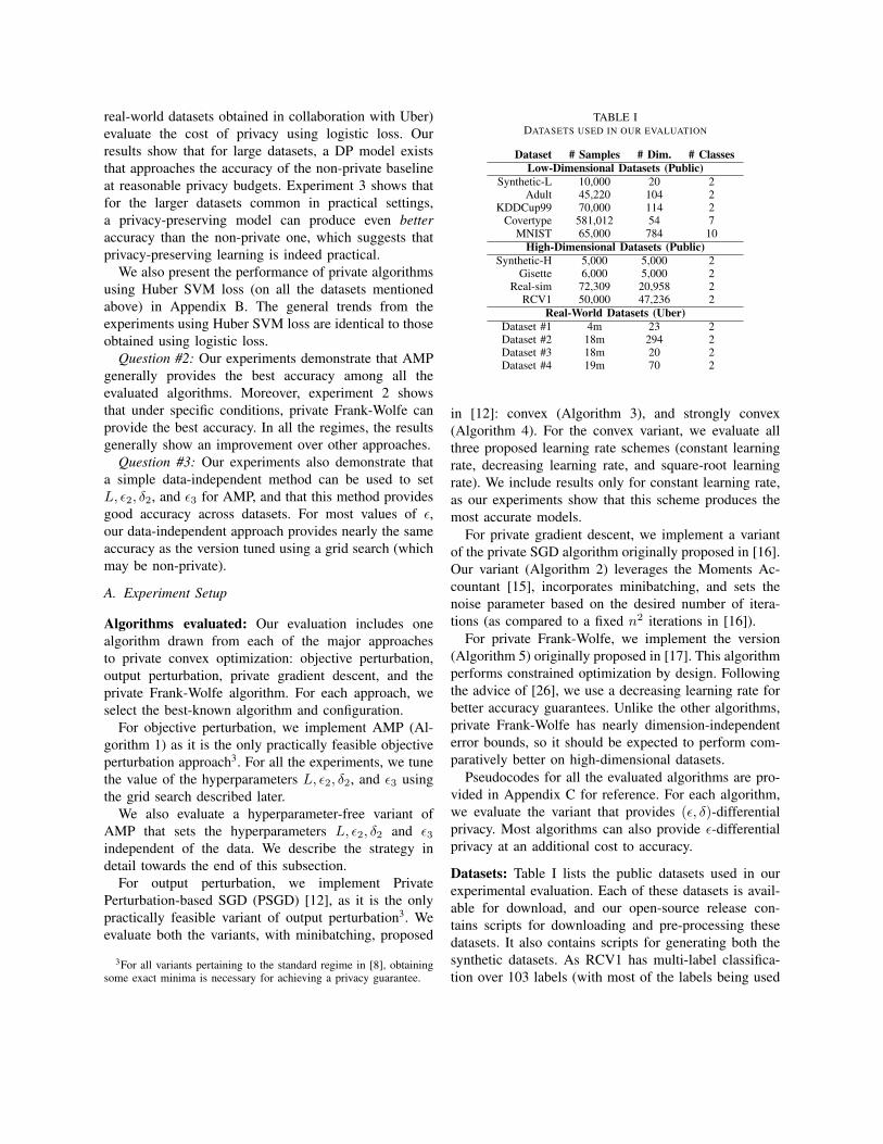
TABLE IDATASETS USED IN OUR EVALUATION

Dataset # Samples # Dim. # ClassesLow-Dimensional Datasets (Public)

Synthetic-L 10,000 20 2Adult 45,220 104 2

KDDCup99 70,000 114 2Covertype 581,012 54 7

MNIST 65,000 784 10High-Dimensional Datasets (Public)

Synthetic-H 5,000 5,000 2Gisette 6,000 5,000 2

Real-sim 72,309 20,958 2RCV1 50,000 47,236 2

Real-World Datasets (Uber)Dataset #1 4m 23 2Dataset #2 18m 294 2Dataset #3 18m 20 2Dataset #4 19m 70 2

in [12]: convex (Algorithm 3), and strongly convex(Algorithm 4). For the convex variant, we evaluate allthree proposed learning rate schemes (constant learningrate, decreasing learning rate, and square-root learningrate). We include results only for constant learning rate,as our experiments show that this scheme produces themost accurate models.

For private gradient descent, we implement a variantof the private SGD algorithm originally proposed in [16].Our variant (Algorithm 2) leverages the Moments Ac-countant [15], incorporates minibatching, and sets thenoise parameter based on the desired number of itera-tions (as compared to a fixed n2 iterations in [16]).

For private Frank-Wolfe, we implement the version(Algorithm 5) originally proposed in [17]. This algorithmperforms constrained optimization by design. Followingthe advice of [26], we use a decreasing learning rate forbetter accuracy guarantees. Unlike the other algorithms,private Frank-Wolfe has nearly dimension-independenterror bounds, so it should be expected to perform com-paratively better on high-dimensional datasets.

Pseudocodes for all the evaluated algorithms are pro-vided in Appendix C for reference. For each algorithm,we evaluate the variant that provides (ε, δ)-differentialprivacy. Most algorithms can also provide ε-differentialprivacy at an additional cost to accuracy.

Datasets: Table I lists the public datasets used in ourexperimental evaluation. Each of these datasets is avail-able for download, and our open-source release con-tains scripts for downloading and pre-processing thesedatasets. It also contains scripts for generating both thesynthetic datasets. As RCV1 has multi-label classifica-tion over 103 labels (with most of the labels being used

for a very small proportion of the dataset), for this datasetwe consider the task of predicting whether a sample iscategorized under the most frequently used label or not.

The selected datasets include both low-dimensionaland high-dimensional datasets. We define low-dimensional datasets to be ones where n � p (wheren is the number of samples and p is the number ofdimensions). High-dimensional datasets are definedas those for which n and p are on roughly the samescale, i.e. n ≤ p (or nearly so). We consider theSynthetic-H, Gisette, Real-sim, and RCV1 datasets tobe high-dimensional.

To obtain training and testing sets, we randomlyshuffle the dataset, take the first 80% as the training set,and the remaining 20% as the testing set.

Sample clipping: Each of the algorithms we evalu-ate has the requirement that the loss have a Lipschitzconstant. We can enforce this requirement for the lossfunctions we consider by bounding the norm for eachsample. We can accomplish this by pre-processing thedataset, but it must be done carefully to preserve DP.

For all the algorithms except private Frank-Wolfe,to make the loss have an L2-Lipschitz constant L, webound the influence of each sample (xi, yi) by clip-ping the feature vector xi to

(xi ·min

(1, L‖xi‖

)). This

transformation is independent of other samples, and thuspreserves DP; it has also been previously used, e.g. in[15]. As the private Frank-Wolfe algorithm requires theloss to have a relaxed L1-Lipschitz constant L, it suffices(using Theorem 1 from [41]) to bound the L∞-norm ofeach sample (xi, yi) by L. We achieve this by clippingeach dimension xi,j , where j ∈ [d], to min (xi,j , L).

Hyperparameters: Each of the evaluated algorithmshas at least one hyperparameter. The values for thesehyperparameters should be tuned to provide the bestaccuracy, but the tuning should be done privately in orderto guarantee end-to-end differential privacy. Although anumber of differentially private hyperparameter tuningalgorithms have been proposed [8], [14], [15] to addressthis problem, they add more variance in the performanceof each algorithm, thus making it more difficult tocompare the performance across different algorithms.

In order to provide a fair comparison between algo-rithms, we use a grid search to determine the best valuefor each hyperparameter. Our grid search considers thehyperparameter values listed in Table II. In addition tothe standard algorithm hyperparameters (Λ, η, T, k), wetune the clipping parameter L used in pre-processingthe datasets, and the constraint on the model space

TABLE IIHYPERPARAMETER & PRIVACY PARAMETER VALUES

Hyperparameter Values ConsideredΛ (regularization factor) 10−5, 10−4, 10−3, 10−2, 0

η (learning rate) 0.001, 0.01, 0.1, 1T (number of iterations) 5, 10, 100, 1000, 5000

k (minibatch size) 50, 100, 300L (clipping threshold) 0.1, 1, 10, 100C (model constraint) 1, 10

f (output budget fraction) 0.001, 0.01, 0.1, 0.5f1 (privacy budget fraction) 0.9, 0.92, 0.95, 0.98, 0.99

Privacy Parameter Values Consideredε 10−2, 10−

32 , 10−1, 10−

12 ,

100, 1012 , 101

δ 1n2

used by private Frank-Wolfe, Private SGD when usingregularized loss, and Private strongly convex PSGD. Theparameter C controls the size of the L1/L2-ball fromwhich models are selected by private Frank-Wolfe/theother algorithms respectively. For AMP, we set ε2 = f ·ε,δ2 = f ·δ, and tune for f . Here, f denotes the fraction ofthe budget (ε, δ) that is allocated to (ε2, δ2). Also, sincethe valid range of the hyperparameter ε3 depends on thevalue of ε1, we set ε3 = f1 · ε1, and tune for f1. We alsoensure that the constraint on ε3 in Line 3 of Algorithm 1is satisfied. Note that tuning hyperparameters may benon-private, but it enables a direct comparison of thealgorithms themselves.

We consider a range of values for the privacy pa-rameter ε. Following Wu et al. [12], we set the privacyparameter δ = 1

n2 , where n is the size of the trainingdata. The complete set of values considered is listedin Table II. For multiclass classification datasets suchas MNIST and Covertype, we implement the one-vs-allstrategy by training a binary classifier for each class, andsplit ε and δ equally among the binary classifiers so thatwe can achieve an overall (ε, δ)-DP guarantee by usinggeneral composition [40].

Algorithm Implementations: The implementationsused in our evaluation correspond to the pseudocodelistings in Appendix C, are written in Python, andare available in our open source release [13]. For Ap-proximate Minima Perturbation, we define the loss andgradient according to Algorithm 1, and leverage SciPy’sminimize procedure to find the approximate minima.

For all datasets, our implementation is able to achieveγ = 1

n2 , where n is the size of the training data. Forlow-dimensional datasets, our implementation of AMPuses SciPy’s BFGS solver, for which we can specifythe desired norm bound γ. The BFGS algorithm stores

the full Hessian of the objective, which does not fit inmemory for the sparse high-dimensional datasets in ourstudy. For these, we define an alternative low-memoryimplementation using SciPy’s L-BFGS-B solver, whichdoes not store the full Hessian.

Experiment procedure: Our experiment setup is de-signed to find the best possible accuracy achievable fora given setting of the privacy parameters. To ensure afair comparison, we begin every run of each algorithmwith the initial model 0p. Because each of the evaluatedalgorithms introduces randomness due to noise, we train10 independent models for each combination of thehyperparameter setting. We report the mean accuracy andstandard deviation for the combination of the hyperpa-rameter setting with the highest mean accuracy over the10 independent runs.4

Differences with the setting in [12]: Although boththe studies have 3 datasets in common (Covertype, KD-DCup99, and MNIST), our setting is slightly differentfrom [12] for all 3 of them. For Covertype, our studyuses all 7 classes, while [12] uses a binary version. ForKDDCup99, we use a 10% sample of the full dataset (asin [42]), while [12] uses the full dataset. For MNIST,we use all 784 dimensions, while [12] uses randomprojection to reduce the dimensionality to 50.

The results we obtain for both the variants of thePrivate PSGD algorithm [12] are based on faithful im-plementations of those algorithms. We tune the hyperpa-rameters for both, using the grid search described earlier.

Non-private baseline: Note that one of the main objec-tives of this study is to determine the cost of privacyin practice for convex optimization. Hence, to providea point of comparison for our results, we also train anon-private baseline model for each experiment. We useScikit-learn’s LogisticRegression class to trainthis model on the same training data as the privatealgorithms, and test its accuracy on the same testing dataas the private algorithms. We do not perform sampleclipping when training this model.

Strategy for Hyperparameter-free Approximate Min-ima Perturbation: Now, we describe a data-independentapproach for setting Approximate Minima Perturbation’sonly hyperparameters, L, ε2, δ2, and ε3, for both the lossfunctions we consider (see Section V-B). For L, we findthat setting L = 1 achieves a good trade-off between

4The results shown are for hyperparameters tuned via the mean testset accuracy. Since all the considered algorithms aim to minimize theempirical loss, we also conducted experiments by tuning via the meantraining set accuracy. Both settings provided visibly identical results.

the amount of noise added for perturbing the objective,and the information loss after sample clipping across alldatasets. Next, we consider only the synthetically gener-ated datasets for setting the hyperparameters specific toAMP. Fixing γ = 1

n2 , we find that setting ε2 = 0.01 · εand δ2 = 0.01 · δ achieves a good trade-off betweenthe budget for perturbing the objective, and the amountof noise that its approximate minima can tolerate. Forsetting ε3, we consider two separate cases:• For ε1 = 0.99 · ε, and ε3 = f1 · ε1, we see that

setting f1 = 0.99 for ε1 = 0.0099, f1 = 0.95for ε1 ∈ {0.0313, 0.099}, and f1 = 0.9 for ε1 ∈{0.313, 0.99, 3.13, 9.99} yields a good accuracy forSynthetic-L. Hence, we observe that for very lowvalues of ε1, a good accuracy is yielded by ε3 closeto ε1 (i.e., most of the budget is used to reduce thescale of the noise, and the influence of regularizationis kept large). As ε1 increases, we see that it is morebeneficial to reduce the effects of regularization. Wefit a basic polynomial curve of the form y = a+bx−c,where a, b, c > 0, to the above-stated values to geta dependence of f1 (the privacy budget fraction) interms of ε1. We combine it with the lower boundimposed on f1 by Theorem 1 (for instance, we requiref1 ≥ 0.9 for ε1 = 9.99) to obtain the following data-independent relationship between ε1 and ε3 for low-dimensional datasets:

ε3 = max

{min

{0.887 +

0.019

ε0.3731

, 0.99

}, 1− 0.99

ε1

}· ε1

• For Synthetic-H, we see that setting f1 = 0.97 yieldsa good accuracy for all the values of ε1 considered.Thus, combining it with the lower bound imposed onf1 by Theorem 1, we obtain the following relationshipfor high-dimensional datasets:

ε3 = max

{0.97, 1− 0.99

ε1

}· ε1

Note that the results for this strategy are consistent forboth loss functions across all the public and the real-world datasets considered, none of which were usedin defining the strategy except for setting the Lipschitzconstant L of the loss. They can be considered to beeffectively serving as test-cases for the strategy.

B. Loss Functions

Our evaluation considers the loss functions for twocommonly used models: logistic regression and HuberSVM. This section contains results for logistic regres-sion; results for Huber SVM are available in Appendix B.

Logistic regression: The L2-regularized logistic regres-sion loss function on a sample (x, y) with y ∈ {1,−1}is `(θ, (x, y)) = ln(1 + exp(−y〈θ, x〉)) + Λ

2 ‖θ‖2.

Our experiments consider both the regularized and un-regularized (i.e., Λ = 0) settings. The un-regularizedversion has L2-Lipschitz constant L when for each sam-ple x, ‖x‖ ≤ L. It is also L2-smooth. The regularizedversion has L2-Lipschitz constant L+ΛC when for eachsample x, ‖x‖ ≤ L, and for each model θ, ‖θ‖ ≤ C. Itis also (L2 + Λ)-smooth, and Λ-strongly convex.

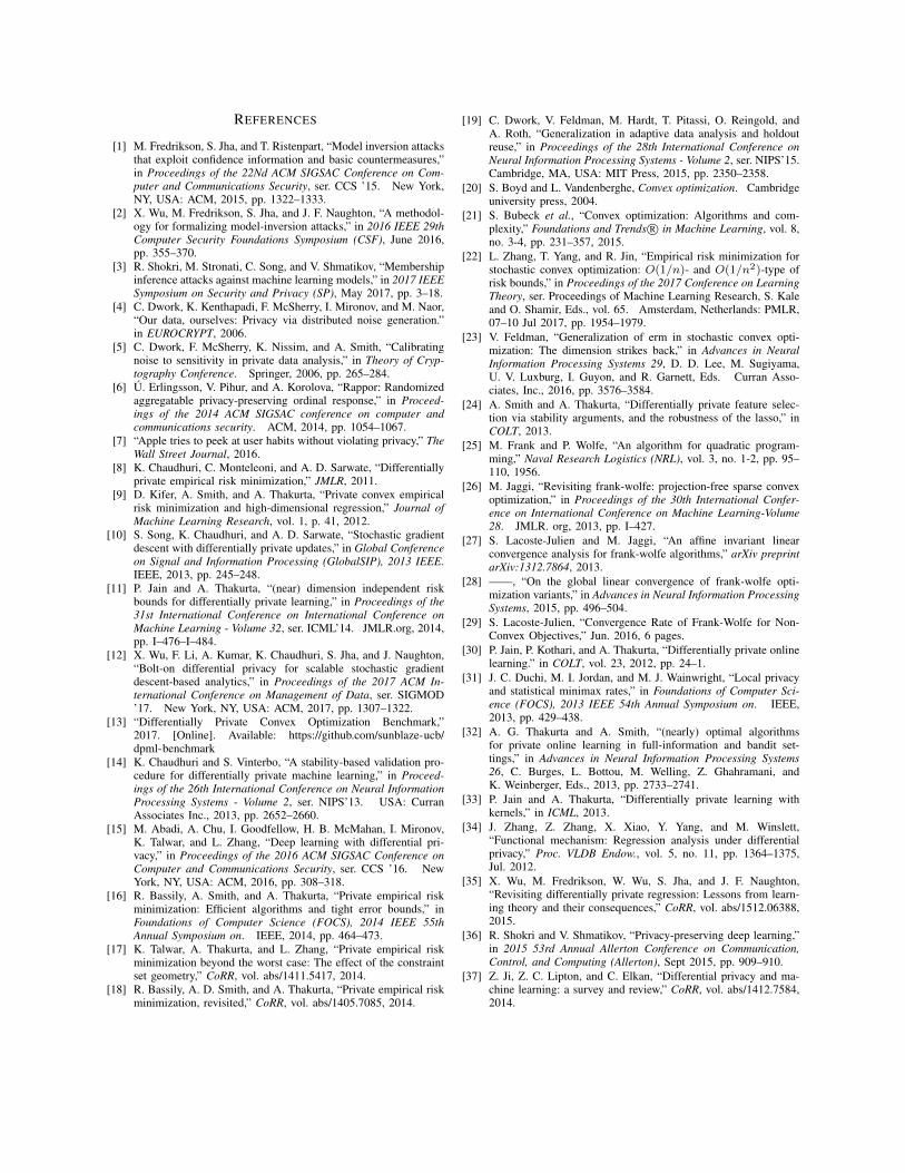
C. Experiment 1: Low-dimensional Datasets

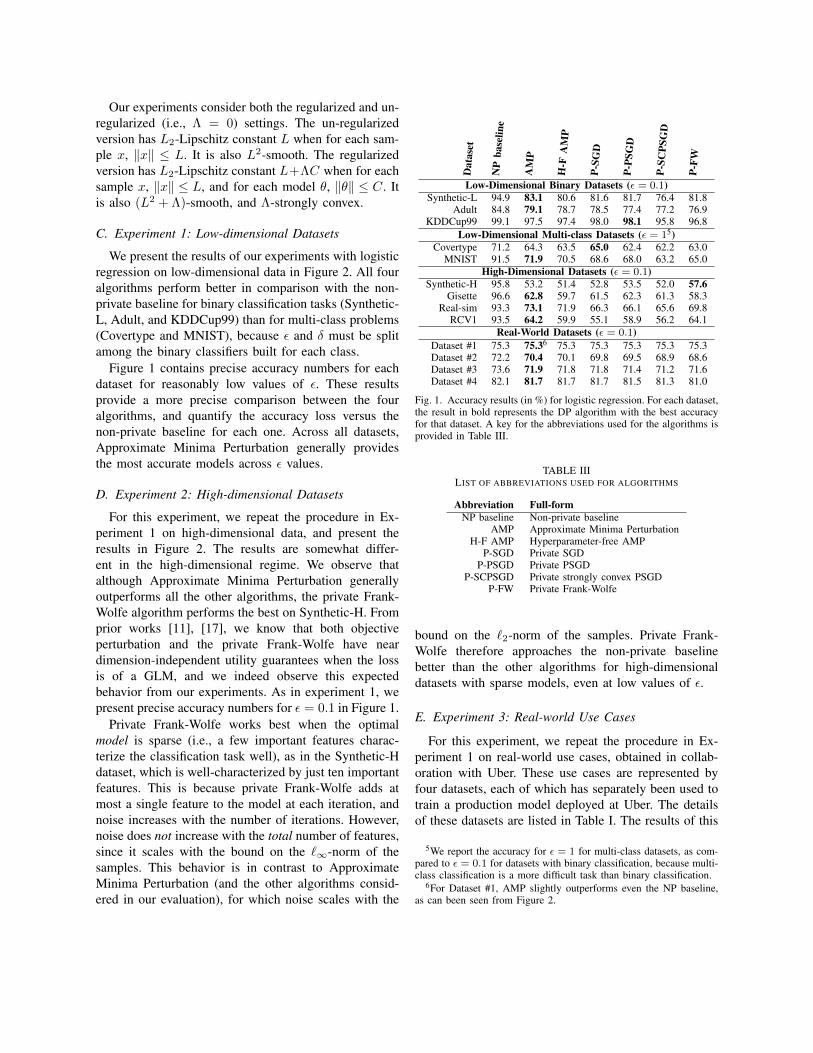
We present the results of our experiments with logisticregression on low-dimensional data in Figure 2. All fouralgorithms perform better in comparison with the non-private baseline for binary classification tasks (Synthetic-L, Adult, and KDDCup99) than for multi-class problems(Covertype and MNIST), because ε and δ must be splitamong the binary classifiers built for each class.

Figure 1 contains precise accuracy numbers for eachdataset for reasonably low values of ε. These resultsprovide a more precise comparison between the fouralgorithms, and quantify the accuracy loss versus thenon-private baseline for each one. Across all datasets,Approximate Minima Perturbation generally providesthe most accurate models across ε values.

D. Experiment 2: High-dimensional Datasets

For this experiment, we repeat the procedure in Ex-periment 1 on high-dimensional data, and present theresults in Figure 2. The results are somewhat differ-ent in the high-dimensional regime. We observe thatalthough Approximate Minima Perturbation generallyoutperforms all the other algorithms, the private Frank-Wolfe algorithm performs the best on Synthetic-H. Fromprior works [11], [17], we know that both objectiveperturbation and the private Frank-Wolfe have neardimension-independent utility guarantees when the lossis of a GLM, and we indeed observe this expectedbehavior from our experiments. As in experiment 1, wepresent precise accuracy numbers for ε = 0.1 in Figure 1.

Private Frank-Wolfe works best when the optimalmodel is sparse (i.e., a few important features charac-terize the classification task well), as in the Synthetic-Hdataset, which is well-characterized by just ten importantfeatures. This is because private Frank-Wolfe adds atmost a single feature to the model at each iteration, andnoise increases with the number of iterations. However,noise does not increase with the total number of features,since it scales with the bound on the `∞-norm of thesamples. This behavior is in contrast to ApproximateMinima Perturbation (and the other algorithms consid-ered in our evaluation), for which noise scales with the

Dat

aset

NP

base

line

AM

P

H-F

AM

P

P-SG

D

P-PS

GD

P-SC

PSG

D

P-FW

Low-Dimensional Binary Datasets (ε = 0.1)Synthetic-L 94.9 83.1 80.6 81.6 81.7 76.4 81.8

Adult 84.8 79.1 78.7 78.5 77.4 77.2 76.9KDDCup99 99.1 97.5 97.4 98.0 98.1 95.8 96.8

Low-Dimensional Multi-class Datasets (ε = 15)Covertype 71.2 64.3 63.5 65.0 62.4 62.2 63.0

MNIST 91.5 71.9 70.5 68.6 68.0 63.2 65.0High-Dimensional Datasets (ε = 0.1)

Synthetic-H 95.8 53.2 51.4 52.8 53.5 52.0 57.6Gisette 96.6 62.8 59.7 61.5 62.3 61.3 58.3

Real-sim 93.3 73.1 71.9 66.3 66.1 65.6 69.8RCV1 93.5 64.2 59.9 55.1 58.9 56.2 64.1

Real-World Datasets (ε = 0.1)Dataset #1 75.3 75.36 75.3 75.3 75.3 75.3 75.3Dataset #2 72.2 70.4 70.1 69.8 69.5 68.9 68.6Dataset #3 73.6 71.9 71.8 71.8 71.4 71.2 71.6Dataset #4 82.1 81.7 81.7 81.7 81.5 81.3 81.0

Fig. 1. Accuracy results (in %) for logistic regression. For each dataset,the result in bold represents the DP algorithm with the best accuracyfor that dataset. A key for the abbreviations used for the algorithms isprovided in Table III.

TABLE IIILIST OF ABBREVIATIONS USED FOR ALGORITHMS

Abbreviation Full-formNP baseline Non-private baseline

AMP Approximate Minima PerturbationH-F AMP Hyperparameter-free AMP

P-SGD Private SGDP-PSGD Private PSGD

P-SCPSGD Private strongly convex PSGDP-FW Private Frank-Wolfe

bound on the `2-norm of the samples. Private Frank-Wolfe therefore approaches the non-private baselinebetter than the other algorithms for high-dimensionaldatasets with sparse models, even at low values of ε.

E. Experiment 3: Real-world Use Cases

For this experiment, we repeat the procedure in Ex-periment 1 on real-world use cases, obtained in collab-oration with Uber. These use cases are represented byfour datasets, each of which has separately been used totrain a production model deployed at Uber. The detailsof these datasets are listed in Table I. The results of this

5We report the accuracy for ε = 1 for multi-class datasets, as com-pared to ε = 0.1 for datasets with binary classification, because multi-class classification is a more difficult task than binary classification.

6For Dataset #1, AMP slightly outperforms even the NP baseline,as can been seen from Figure 2.

10 2 10 1 100 101

Epsilon

50

60

70

80

90Ac

cura

cy (%

)

10 2 10 1 100 101

Epsilon

72.5

75.0

77.5

80.0

82.5

85.0

Accu

racy

(%)

10 2 10 1 100 101

Epsilon

80

85

90

95

100

Accu

racy

(%)

Synthetic-L (Low-Dim) Adult (Low-Dim) KDDCup99 (Low-Dim)

10 2 10 1 100 101

Epsilon

50

55

60

65

70

Accu

racy

(%)

10 2 10 1 100 101

Epsilon

20

40

60

80

Accu

racy

(%)

10 2 10 1 100 101

Epsilon

0.5

0.6

0.7

0.8

0.9

Accu

racy

Covertype (Low-Dim) MNIST (Low-Dim) Synthetic-H (High-Dim)

10 2 10 1 100 101

Epsilon

50

60

70

80

90

Accu

racy

(%)

10 2 10 1 100 101

Epsilon

50

60

70

80

90

Accu

racy

(%)

10 2 10 1 100 101

Epsilon

50

60

70

80

90

Accu

racy

(%)

Gisette (High-Dim) Real-sim (High-Dim) RCV-1 (High-Dim)

10 2 10 1 100 101

Epsilon

75.30

75.32

75.34

Accu

racy

(%)

10 2 10 1 100 101

Epsilon

60

65

70

Accu

racy

(%)

10 2 10 1 100 101

Epsilon

71

72

73

74

Accu

racy

(%)

Dataset #1 (Real-World) Dataset #2 (Real-World) Dataset #3 (Real-World)

10 2 10 1 100 101

Epsilon

80.0

80.5

81.0

81.5

82.0

Accu

racy

(%)

10 2 10 1 100 101

Epsilon

0.80

0.85

0.90

0.95

1.00

Accu

racy

Non-private baselineApproximate Minima PerturbationHyperparameter-free Approximate Minima PerturbationPrivate SGDPrivate PSGDPrivate Strongly-convex PSGDPrivate Frank-Wolfe

Dataset #4 (Real-World) Color-coded Legend for all the plotsFig. 2. Accuracy results for logistic regression on low-dimensional, high-dimensional and real-world datasets. Horizontal axis depicts varyingvalues of ε; vertical axis shows accuracy (in %) on the testing set.

experiment are depicted in Figure 2, with more preciseresults for ε = 0.1 in Figure 1.

The real-world datasets are much larger than thedatasets considered in Experiment 1. The difference inscale is reflected in the results: all of the algorithmsconverge to the non-private baseline for very low valuesof ε. These results suggest that in many practical settings,the cost of privacy is negligible. In fact, for Dataset#1, some differentially private models exhibit a slightlyhigher accuracy than the non-private baseline for awide range of ε. For instance, even Hyperparameter-free AMP, which is end-to-end differentially privateas there is no tuning involved, yields an accuracy of75.34% for ε = 0.1 versus the non-private baseline of75.33%. Some prior works [18], [19] have theorized thatdifferential privacy could act as a type of regularizationfor the system, and improve the generalization error; thisempirical result of ours aligns with this claim.

F. Discussion

For large datasets, the cost of privacy is low. Ourresults confirm the expectation that very accurate dif-ferentially private models exist for large datasets. Evenfor relatively small datasets like Adult and KDDCup99(where n < 100, 000), our results show that a differen-tially private model has accuracy within 6% of the non-private baseline even for a conservative privacy settingof ε = 0.1.

For all the larger real-world datasets (n > 1m),the accuracy of the best differentially private model iswithin 4% of the non-private baseline even for the mostconservative privacy value considered (ε = 0.01). Forε = 0.1, it is within 2% of the baseline for two of thesedatasets, essentially identical to the baseline for one ofthem, and even slightly higher than the baseline for one.

These results suggest that for realistic deploymentson large datasets (n > 1m, and low-dimensional), adifferentially private model can be deployed withoutmuch loss in accuracy.

Approximate Minima Perturbation almost alwaysprovides the best accuracy, and is easily deployable inpractice. Our results in all the experiments demonstratethat among the available algorithms for differentially pri-vate convex optimization, our Approximate Minima Per-turbation approach almost always produces models withthe best accuracy. For four of the five low-dimensionaldatasets, and all the public high-dimensional datasets weconsidered, Approximate Minima Perturbation providedconsistently better accuracy than the other algorithms.Under some conditions like high-dimensionality of the

datasets, and sparsity of the optimal predictive modelfor it, private Frank-Wolfe does give the best perfor-mance. Unlike Approximate Minima Perturbation, how-ever, no hyperparameter-free variant of private Frank-Wolfe exists—and suboptimal hyperparameter valuescan reduce accuracy significantly for this algorithm.

As mentioned earlier, Approximate Minima Perturba-tion also has important properties that enable its practicaldeployment. It can leverage any off-the-shelf optimizeras a black box, allowing implementations to use existingscalable optimizers (our implementation uses Scipy’sminimize). None of the other evaluated algorithmshave these properties.

Hyperparameter-free Approximate Minima Pertur-bation provides good utility. As demonstrated by ourexperimental results, AMP can be deployed without tun-ing hyperparameters, at little cost to accuracy. Our data-independent approach therefore enables deployment—without significant loss of accuracy—in practical settingswhere public data may not be available for tuning.

VI. CONCLUSION

This paper takes two important steps towards practi-cal differentially private convex optimization. We havepresented Approximate Minima Perturbation, a novelalgorithm for differentially private convex optimizationthat does not require the optimization process to reachthe true minima. It can leverage any off-the-shelf solver,and can be employed without hyperparameter tuning.Therefore, it is amenable to be deployed in practice.

We have also performed an extensive empirical eval-uation of state-of-the-art approaches for differentiallyprivate convex optimization. To encourage the furtherdevelopment and deployment, we have released theimplementations used in our evaluation, and the bench-marking scripts used to obtain the datasets and performthe experiments. This benchmark provides a standardpoint of comparison for further advances in differentiallyprivate convex optimization.

VII. ACKNOWLEDGEMENTS

The authors would like to thank Adam Smith forthe discussions regarding the main privacy proof ofAMP, and the anonymous reviewers for their help-ful comments. This material is in part based uponwork supported by NSF CCF-1740850, DARPA contract#N66001-15-C-4066, the Center for Long-Term Cyber-security, and Berkeley Deep Drive. Any opinions, find-ings, conclusions, or recommendations expressed in thismaterial are those of the authors, and do not necessarilyreflect the views of the sponsors.

REFERENCES

[1] M. Fredrikson, S. Jha, and T. Ristenpart, “Model inversion attacksthat exploit confidence information and basic countermeasures,”in Proceedings of the 22Nd ACM SIGSAC Conference on Com-puter and Communications Security, ser. CCS ’15. New York,NY, USA: ACM, 2015, pp. 1322–1333.

[2] X. Wu, M. Fredrikson, S. Jha, and J. F. Naughton, “A methodol-ogy for formalizing model-inversion attacks,” in 2016 IEEE 29thComputer Security Foundations Symposium (CSF), June 2016,pp. 355–370.

[3] R. Shokri, M. Stronati, C. Song, and V. Shmatikov, “Membershipinference attacks against machine learning models,” in 2017 IEEESymposium on Security and Privacy (SP), May 2017, pp. 3–18.

[4] C. Dwork, K. Kenthapadi, F. McSherry, I. Mironov, and M. Naor,“Our data, ourselves: Privacy via distributed noise generation.”in EUROCRYPT, 2006.

[5] C. Dwork, F. McSherry, K. Nissim, and A. Smith, “Calibratingnoise to sensitivity in private data analysis,” in Theory of Cryp-tography Conference. Springer, 2006, pp. 265–284.

[6] U. Erlingsson, V. Pihur, and A. Korolova, “Rappor: Randomizedaggregatable privacy-preserving ordinal response,” in Proceed-ings of the 2014 ACM SIGSAC conference on computer andcommunications security. ACM, 2014, pp. 1054–1067.

[7] “Apple tries to peek at user habits without violating privacy,” TheWall Street Journal, 2016.

[8] K. Chaudhuri, C. Monteleoni, and A. D. Sarwate, “Differentiallyprivate empirical risk minimization,” JMLR, 2011.

[9] D. Kifer, A. Smith, and A. Thakurta, “Private convex empiricalrisk minimization and high-dimensional regression,” Journal ofMachine Learning Research, vol. 1, p. 41, 2012.

[10] S. Song, K. Chaudhuri, and A. D. Sarwate, “Stochastic gradientdescent with differentially private updates,” in Global Conferenceon Signal and Information Processing (GlobalSIP), 2013 IEEE.IEEE, 2013, pp. 245–248.

[11] P. Jain and A. Thakurta, “(near) dimension independent riskbounds for differentially private learning,” in Proceedings of the31st International Conference on International Conference onMachine Learning - Volume 32, ser. ICML’14. JMLR.org, 2014,pp. I–476–I–484.

[12] X. Wu, F. Li, A. Kumar, K. Chaudhuri, S. Jha, and J. Naughton,“Bolt-on differential privacy for scalable stochastic gradientdescent-based analytics,” in Proceedings of the 2017 ACM In-ternational Conference on Management of Data, ser. SIGMOD’17. New York, NY, USA: ACM, 2017, pp. 1307–1322.

[13] “Differentially Private Convex Optimization Benchmark,”2017. [Online]. Available: https://github.com/sunblaze-ucb/dpml-benchmark

[14] K. Chaudhuri and S. Vinterbo, “A stability-based validation pro-cedure for differentially private machine learning,” in Proceed-ings of the 26th International Conference on Neural InformationProcessing Systems - Volume 2, ser. NIPS’13. USA: CurranAssociates Inc., 2013, pp. 2652–2660.

[15] M. Abadi, A. Chu, I. Goodfellow, H. B. McMahan, I. Mironov,K. Talwar, and L. Zhang, “Deep learning with differential pri-vacy,” in Proceedings of the 2016 ACM SIGSAC Conference onComputer and Communications Security, ser. CCS ’16. NewYork, NY, USA: ACM, 2016, pp. 308–318.

[16] R. Bassily, A. Smith, and A. Thakurta, “Private empirical riskminimization: Efficient algorithms and tight error bounds,” inFoundations of Computer Science (FOCS), 2014 IEEE 55thAnnual Symposium on. IEEE, 2014, pp. 464–473.

[17] K. Talwar, A. Thakurta, and L. Zhang, “Private empirical riskminimization beyond the worst case: The effect of the constraintset geometry,” CoRR, vol. abs/1411.5417, 2014.

[18] R. Bassily, A. D. Smith, and A. Thakurta, “Private empirical riskminimization, revisited,” CoRR, vol. abs/1405.7085, 2014.

[19] C. Dwork, V. Feldman, M. Hardt, T. Pitassi, O. Reingold, andA. Roth, “Generalization in adaptive data analysis and holdoutreuse,” in Proceedings of the 28th International Conference onNeural Information Processing Systems - Volume 2, ser. NIPS’15.Cambridge, MA, USA: MIT Press, 2015, pp. 2350–2358.

[20] S. Boyd and L. Vandenberghe, Convex optimization. Cambridgeuniversity press, 2004.

[21] S. Bubeck et al., “Convex optimization: Algorithms and com-plexity,” Foundations and Trends R© in Machine Learning, vol. 8,no. 3-4, pp. 231–357, 2015.

[22] L. Zhang, T. Yang, and R. Jin, “Empirical risk minimization forstochastic convex optimization: O(1/n)- and O(1/n2)-type ofrisk bounds,” in Proceedings of the 2017 Conference on LearningTheory, ser. Proceedings of Machine Learning Research, S. Kaleand O. Shamir, Eds., vol. 65. Amsterdam, Netherlands: PMLR,07–10 Jul 2017, pp. 1954–1979.

[23] V. Feldman, “Generalization of erm in stochastic convex opti-mization: The dimension strikes back,” in Advances in NeuralInformation Processing Systems 29, D. D. Lee, M. Sugiyama,U. V. Luxburg, I. Guyon, and R. Garnett, Eds. Curran Asso-ciates, Inc., 2016, pp. 3576–3584.

[24] A. Smith and A. Thakurta, “Differentially private feature selec-tion via stability arguments, and the robustness of the lasso,” inCOLT, 2013.

[25] M. Frank and P. Wolfe, “An algorithm for quadratic program-ming,” Naval Research Logistics (NRL), vol. 3, no. 1-2, pp. 95–110, 1956.

[26] M. Jaggi, “Revisiting frank-wolfe: projection-free sparse convexoptimization,” in Proceedings of the 30th International Confer-ence on International Conference on Machine Learning-Volume28. JMLR. org, 2013, pp. I–427.

[27] S. Lacoste-Julien and M. Jaggi, “An affine invariant linearconvergence analysis for frank-wolfe algorithms,” arXiv preprintarXiv:1312.7864, 2013.

[28] ——, “On the global linear convergence of frank-wolfe opti-mization variants,” in Advances in Neural Information ProcessingSystems, 2015, pp. 496–504.

[29] S. Lacoste-Julien, “Convergence Rate of Frank-Wolfe for Non-Convex Objectives,” Jun. 2016, 6 pages.

[30] P. Jain, P. Kothari, and A. Thakurta, “Differentially private onlinelearning.” in COLT, vol. 23, 2012, pp. 24–1.

[31] J. C. Duchi, M. I. Jordan, and M. J. Wainwright, “Local privacyand statistical minimax rates,” in Foundations of Computer Sci-ence (FOCS), 2013 IEEE 54th Annual Symposium on. IEEE,2013, pp. 429–438.

[32] A. G. Thakurta and A. Smith, “(nearly) optimal algorithmsfor private online learning in full-information and bandit set-tings,” in Advances in Neural Information Processing Systems26, C. Burges, L. Bottou, M. Welling, Z. Ghahramani, andK. Weinberger, Eds., 2013, pp. 2733–2741.

[33] P. Jain and A. Thakurta, “Differentially private learning withkernels,” in ICML, 2013.

[34] J. Zhang, Z. Zhang, X. Xiao, Y. Yang, and M. Winslett,“Functional mechanism: Regression analysis under differentialprivacy,” Proc. VLDB Endow., vol. 5, no. 11, pp. 1364–1375,Jul. 2012.

[35] X. Wu, M. Fredrikson, W. Wu, S. Jha, and J. F. Naughton,“Revisiting differentially private regression: Lessons from learn-ing theory and their consequences,” CoRR, vol. abs/1512.06388,2015.

[36] R. Shokri and V. Shmatikov, “Privacy-preserving deep learning,”in 2015 53rd Annual Allerton Conference on Communication,Control, and Computing (Allerton), Sept 2015, pp. 909–910.

[37] Z. Ji, Z. C. Lipton, and C. Elkan, “Differential privacy and ma-chine learning: a survey and review,” CoRR, vol. abs/1412.7584,2014.

[38] A. Nikolov, K. Talwar, and L. Zhang, “The geometry of differen-tial privacy: The sparse and approximate cases,” in Proceedings ofthe Forty-fifth Annual ACM Symposium on Theory of Computing,ser. STOC ’13. New York, NY, USA: ACM, 2013, pp. 351–360.

[39] P. Billingsley, Probability and Measure, ser. Wiley Series inProbability and Statistics. Wiley, 1995.

[40] C. Dwork, A. Roth et al., “The algorithmic foundations of differ-ential privacy,” Foundations and Trends in Theoretical ComputerScience, vol. 9, no. 3-4, pp. 211–407, 2014.

[41] R. Paulavicius and J. Zilinskas, “Analysis of different norms andcorresponding lipschitz constants for global optimization,” UkioTechnologinis ir Ekonominis Vystymas, vol. 12, no. 4, pp. 301–306, 2006.

[42] K. Chaudhuri, C. Monteleoni, and A. D. Sarwate, “Differentiallyprivate empirical risk minimization,” Journal of Machine Learn-ing Research, vol. 12, no. Mar, pp. 1069–1109, 2011.

[43] S. Dasgupta and L. Schulman, “A probabilistic analysis of emfor mixtures of separated, spherical gaussians,” JMLR, 2007.

[44] K. Talwar, A. Thakurta, and L. Zhang, “Nearly optimal privatelasso,” in NIPS, 2015.

APPENDIX

A. Omitted ProofsHere, we provide a proof for the utility guarantee

of Algorithm 1, which is provided in Theorem 2. Forbounding the expected risk of the algorithm, we firstneed to bound its empirical risk (Lemma A.1).

Lemma A.1 (Empirical Risk). Let θ be the minimizer

of the objective function L(θ;D) = 1n

n∑i=1

`(θ; di),

and θmin be the minimizer of the objective functionLpriv(θ;D) = L(θ;D) + Λ

2n‖θ‖2 + bT1 θ, where b1 is

as defined in Algorithm 1. Also, let θout be the outputof Algorithm 1. We have:

L(θout;D)− L(θ;D) ≤ L(nγ

Λ+ ‖b2‖

)+

Λ‖θ‖2

2n+

2n‖b1‖2

Λ.

Proof. We have

L(θout;D)− L(θ;D) = (L(θout;D)− L(θmin;D))

+(L(θmin;D)− L(θ;D)

)(4)

First, we will bound (L(θout;D)− L(θmin;D)). Wehave:

L(θout;D)− L(θmin;D) ≤ |L(θout;D)− L(θmin;D)|≤ L‖θout − θmin‖= L‖θapprox − θmin + b2‖≤ L‖θapprox − θmin‖

+ L‖b2‖

≤ L(nγ

Λ+ ‖b2‖

)(5)

The second inequality above follows from the Lipschitzproperty of L(;D). The first equality follows as θout =θmin+(θapprox−θmin+b2), whereas the last inequalityfollows from inequality 3.

Next, we bound(L(θmin;D)− L(θ;D)

)on the

lines of the proof of Lemma 3 in [9]. Let θ# =arg minθ∈Rp L#(θ;D), where L#(θ;D) = L(θ;D) +Λ2n‖θ‖

2. As a result, Lpriv(θ;D) = L#(θ;D) + bT1 θ.So, we have:

L(θmin;D)− L(θ;D) = L#(θmin;D)− L#(θ#;D)

+ L#(θ#;D)− L#(θ;D)

+Λ‖θ‖2

2n− Λ‖θmin‖2

2n≤ L#(θmin;D)− L#(θ#;D)

+Λ‖θ‖2

2n(6)

The inequality above follows as L#(θ#;D) ≤L#(θ;D).

Let us now bound L#(θmin;D) − L#(θ#;D). Tothis end, we first observe that since Lpriv is Λ

n -stronglyconvex in θ, we have that

Lpriv(θ#;D) ≥ Lpriv(θmin;D)

−∇Lpriv(θmin;D)T (θmin − θ#)

+Λ

2n‖θ# − θmin‖2

= Lpriv(θmin;D) +Λ

2n‖θ# − θmin‖2

(7)

The equality above follows as ‖∇Lpriv(θmin;D)‖ = 0.Substituting the definition of Lpriv(;D) in equality 7,

we get that

L#(θmin;D)− L#(θ#;D) ≤ bT1 (θ# − θmin)

− Λ

2n‖θ# − θmin‖2

(8)

≤ ‖b1‖ · ‖θ# − θmin‖(9)

Inequality 9 above follows by the Cauchy–Schwarzinequality.

Now, since L#(θmin;D)−L#(θ#;D) ≥ 0, it followsfrom inequalities 8 and 9 that

‖b1‖ · ‖θ# − θmin‖ ≥Λ

2n‖θ# − θmin‖2

⇒ ‖θ# − θmin‖ ≤2n‖b1‖

Λ(10)

We get the statement of the lemma from equation 4,and inequalities 5, 6, 9, and 10.

Now, we are ready to prove Theorem 2.

Proof of Theorem 2. The proof is on the lines of theproof of Theorem 4 in [9]. First, let us get a highprobability bound on L(θout;D) − L(θ;D). To thisend, we will first bound ‖b1‖ and ‖b2‖ w.h.p., wherebs ∼ N

(0, σ2

sIp×p)

for s ∈ {1, 2}. Using Lemma 2from [43], we get that w.p. ≥ 1− α

2 ,

‖bs‖ ≤ σs

√2p log

2

α.

Substituting this into Lemma A.1, we get that w.p.≥ 1− α,

L(θout;D)− L(θ;D) ≤ L

(nγ

Λ+ σ2

√2p log

2

α

)

+Λ‖θ‖2

2n+

4nσ21p log 2

α

Λ.

It is easy to see that by making εi = ε2 for

i ∈ {1, 2}, ε3 = max{ε12 , ε1 − 0.99

}, δj =

δ2 for j ∈ {1, 2}, and setting Λ =

Θ

(L√rp log 1/δ

ε‖θ‖+ n‖θ‖

√Lγ√p log 1/δ

ε

)such that it

satisfies the constraint in Step 2 in Algorithm 1, we getthe statement of the theorem.

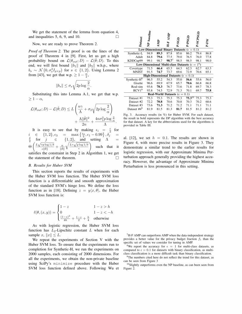
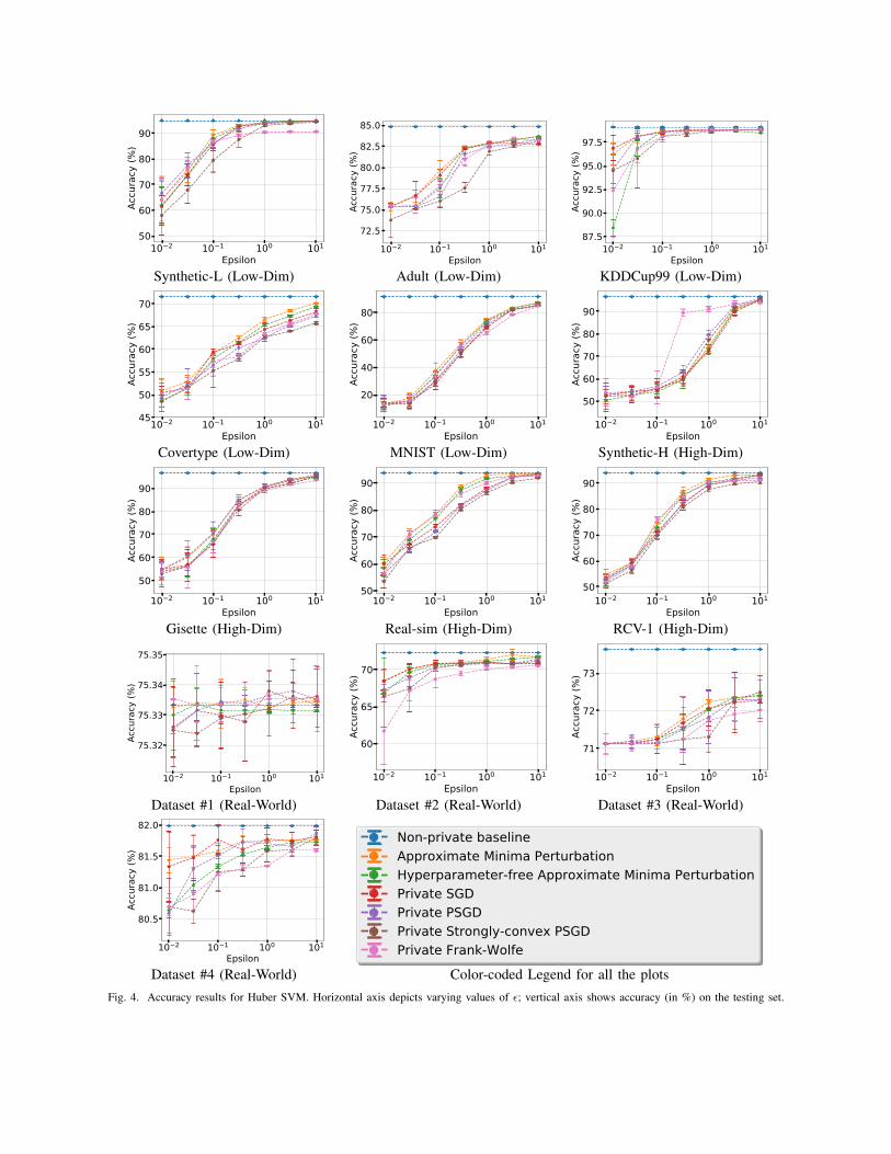
B. Results for Huber SVM

This section reports the results of experiments withthe Huber SVM loss function. The Huber SVM lossfunction is a differentiable and smooth approximationof the standard SVM’s hinge loss. We define the lossfunction as in [18]. Defining z = y〈x, θ〉, the HuberSVM loss function is:

`(θ, (x, y)) =

1− z 1− z > h

0 1− z < −h(1−z)2

4h + 1−z2 + h

4 otherwise

As with logistic regression, the Huber SVM lossfunction has L2-Lipschitz constant L when for eachsample x, ‖x‖ ≤ L.

We repeat the experiments of Section V with theHuber SVM loss. To ensure that the experiments run tocompletion for Synthetic-H, we run the experiments on2000 samples, each consisting of 2000 dimensions. Forall the experiments, we obtain the non-private baselineusing SciPy’s minimize procedure with the HuberSVM loss function defined above. Following Wu et

Dat

aset

NP

base

line

AM

P

H-F

AM

P

P-SG

D

P-PS

GD

P-SC

PSG

D

P-FW

Low-Dimensional Binary Datasets (ε = 0.1)Synthetic-L 94.9 89.3 87.8 85.6 86.2 79.4 86.8

Adult 84.8 79.6 77.5 79.0 76.5 76.0 77.8KDDCup99 99.1 98.7 98.77 98.5 98.5 98.1 98.0

Low-Dimensional Multi-class Datasets (ε = 18)Covertype 71.5 66.4 65.3 64.3 62.3 62.7 63.3

MNIST 91.5 74.7 73.7 69.6 72.9 70.6 65.1High-Dimensional Datasets (ε = 0.1)

Synthetic-H9 96.5 55.2 54.3 55.0 56.6 55.6 56.0Gisette 96.6 69.9 67.9 65.7 70.6 66.8 66.8

Real-sim 93.6 78.3 76.7 73.6 71.8 69.7 78.3RCV19 93.8 74.5 72.9 71.3 70.1 69.7 75.8

Real-World Datasets (ε = 0.1)Dataset #1 75.3 75.3 75.3 75.3 75.310 75.3 75.3Dataset #2 72.2 70.8 70.6 70.8 70.3 70.2 68.6Dataset #3 73.6 71.3 71.2 71.2 71.1 71.1 71.1

Dataset #49 81.9 81.5 81.3 81.7 81.5 81.2 81.2

Fig. 3. Accuracy results (in %) for Huber SVM. For each dataset,the result in bold represents the DP algorithm with the best accuracyfor that dataset. A key for the abbreviations used for the algorithms isprovided in Table III.

al. [12], we set h = 0.1. The results are shown inFigure 4, with more precise results in Figure 3. Theydemonstrate a similar trend to the earlier results forlogistic regression, with our Approximate Minima Per-turbation approach generally providing the highest accu-racy. However, the advantage of Approximate MinimaPerturbation is less pronounced in this setting.

7H-F AMP can outperform AMP when the data-independent strategyprovides a better value for the privacy budget fraction f1 than thespecific set of values we consider for tuning in AMP.

8We report the accuracy for ε = 1 for multi-class datasets, ascompared to ε = 0.1 for datasets with binary classification, as multi-class classification is a more difficult task than binary classification.

9The numbers cited here do not reflect the trend for this dataset, ascan be seen from Figure 3

10Slightly outperforms even the NP baseline, as can been seen fromFigure 2.

10 2 10 1 100 101

Epsilon

50

60

70

80

90Ac

cura

cy (%

)

10 2 10 1 100 101

Epsilon

72.5

75.0

77.5

80.0

82.5

85.0

Accu

racy

(%)

10 2 10 1 100 101

Epsilon

87.5

90.0

92.5

95.0

97.5

Accu

racy

(%)

Synthetic-L (Low-Dim) Adult (Low-Dim) KDDCup99 (Low-Dim)

10 2 10 1 100 101

Epsilon45

50

55

60

65

70

Accu

racy

(%)

10 2 10 1 100 101

Epsilon

20

40

60

80

Accu

racy

(%)

10 2 10 1 100 101

Epsilon

50

60

70

80

90

Accu

racy

(%)

Covertype (Low-Dim) MNIST (Low-Dim) Synthetic-H (High-Dim)

10 2 10 1 100 101

Epsilon

50

60

70

80

90

Accu

racy

(%)

10 2 10 1 100 101

Epsilon

50

60

70

80

90

Accu

racy

(%)

10 2 10 1 100 101

Epsilon

50

60

70

80

90

Accu

racy

(%)

Gisette (High-Dim) Real-sim (High-Dim) RCV-1 (High-Dim)

10 2 10 1 100 101

Epsilon

75.32

75.33

75.34

75.35

Accu

racy

(%)

10 2 10 1 100 101

Epsilon

60

65

70

Accu

racy

(%)

10 2 10 1 100 101

Epsilon

71

72

73

Accu

racy

(%)

Dataset #1 (Real-World) Dataset #2 (Real-World) Dataset #3 (Real-World)

10 2 10 1 100 101

Epsilon

80.5

81.0

81.5

82.0

Accu

racy

(%)

10 2 10 1 100 101

Epsilon

0.80

0.85

0.90

0.95

1.00

Accu

racy

Non-private baselineApproximate Minima PerturbationHyperparameter-free Approximate Minima PerturbationPrivate SGDPrivate PSGDPrivate Strongly-convex PSGDPrivate Frank-Wolfe

Dataset #4 (Real-World) Color-coded Legend for all the plotsFig. 4. Accuracy results for Huber SVM. Horizontal axis depicts varying values of ε; vertical axis shows accuracy (in %) on the testing set.

C. Pseudocodes for Algorithms evaluated in Section V

Algorithm 2: Differentially Private MinibatchStochastic Gradient Descent [16], [15]

Input: Data set: D = {d1, · · · , dn}, loss function:`(θ;Di) with L2-Lipschitz constant L,privacy parameters: (ε, δ), number ofiterations: T , minibatch size: k, learningrate function: η : [T ]→ R.

1 σ2 ← 16L2T log 1δ

n2ε2

2 θ1 = 0p

3 for t = 1 to T-1 do4 s1, · · · , sk ← Sample k samples uniformly with

replacement from D5 bt ∼ N (0, σ2Ip×p)

6 θt+1 = θt − η(t)[( 1k

∑ki=1∇`(θ; si)) + bt]

7 end8 Output θT

Algorithm 3: Differentially Private Permutation-based Stochastic Gradient Descent [12]

Input: Data set: D = {d1, · · · , dn}, loss function:`(θ;Di) with L2-Lipschitz constant L,privacy parameters: (ε, δ), number ofpasses: T , minibatch size: k, constantlearning rate: η.

1 θ ← 0p

2 Let τ be a random permutation of [n]3 for t = 1 to T − 1 do4 for b = 1 to n

k do5 Let s1 = dτ(bk), · · · , sk = dτ(b(k+1)−1)

6 θ ← θ − η( 1k

∑ki=1∇`(θ; si))

7 end8 end9 σ2 ← 8T 2L2η2 log( 2

δ )

k2ε2

10 b ∼ N (0, σ2Ip×p)11 Output θpriv = θ + b

Algorithm 4: Differentially Private Strongly ConvexPermutation-based Stochastic Gradient Descent [12]Input: Data set: D = {d1, · · · , dn}, loss function:

`(θ;Di) that is ξ-strongly convex andβ-smooth with L2-Lipschitz constant L,privacy parameters: (ε, δ), number ofpasses: T , minibatch size: k.

1 θ ← 0p

2 Let τ be a random permutation of [n]3 for t = 1 to T − 1 do4 ηt ← min 1

β ,1ξt

5 for b = 1 to nk do

6 Let s1 = dτ(bk), · · · , sk = dτ(b(k+1)−1)

7 θ ← θ − ηt( 1k

∑ki=1∇`(θ; si))

8 end9 end

10 σ2 ← 8L2 log( 2δ )

ξ2n2ε2

11 b ∼ N (0, σ2Ip×p)12 Output θpriv = θ + b

Algorithm 5: Differentially Private Frank-Wolfe [44]Input: Data set: D = {d1, · · · , dn}, loss function:

L(θ;D) = 1n

n∑i=1

`(θ; di) (with L1-Lipshitz

constant L for `), privacy parameters: (ε, δ),convex set: C = conv(S) with ‖C‖1denoting maxs∈S‖s‖1 and S being the setof corners.

1 Choose an arbitrary θ1 from C

2 σ2 ← 32L2‖C‖21Tlog(1/δ)n2ε2

3 for t = 1 to T-1 do4 ∀s ∈ S, αs ← 〈s,5L(θt;D)〉+ Lap(σ), where

Lap(λ) ∼ 12λe−|x|/λ

5 θt ← arg mins∈S

αs

6 θt+1 ← (1− ηt)θt + ηθt, where ηt = 1t+1

7 end8 Output θpriv = θT