Towards K-Nearest Neighbor Search in Time-DependentSpatial Network Databases ?

Ugur Demiryurek, Farnoush Banaei-Kashani, and Cyrus Shahabi

University of Southern CaliforniaDepartment of Computer Science

Los Angeles, CA 90089-0781[demiryur, banaeika, shahabi]@usc.edu

Abstract. The class of k Nearest Neighbor (kNN) queries in spatial networks isextensively studied in the context of numerous applications. In this paper, for thefirst time we study a generalized form of this problem, called the Time-Dependentk Nearest Neighbor problem (TD-kNN) with which edge-weights are time variable.All existing approaches for kNN search assume that the weight (e.g., travel-time) ofeach edge of the spatial network is constant. However, in real-world edge-weightsare time-dependent (i.e., the arrival-time to an edge determines the actual travel-timeon that edge) and vary significantly in short durations. We study the applicabilityof two baseline solutions for TD-kNN and compare their efficiency via extensiveexperimental evaluations with real-world data-sets, including a variety of large spatialnetworks with real traffic-data recordings.

1 Introduction

With the ever growing popularity of online map services (e.g., Google Maps) and theirwide deployment in hand-held devices (e.g.,iPhone) and car-navigation systems, more andmore users search for geographical points of interests (e.g., restaurants, hospitals) and thecorresponding directions and travel-times to these locations. Consequently, many recentresearch studies (e.g., [23, 5, 18, 16, 22, 2, 12, 13, 17, 24]) focus on developing techniquesto accurately and efficiently compute the distance and route between objects in large road-networks. However, a majority of these studies rely on pre-computation of distances in thenetwork and assume that the cost of traveling each edge of the road-network is constant(e.g., corresponding to the length of the edge).

On the other hand, we are witnessing an increase in the instrumentation of roads inmajor cities for collecting real-time traffic data. For example, we are working with LAMETRO 1 from whom we are receiving real-time traffic data from more than 6500 sensorson various freeways and artillery roads in Los Angeles (LA) county. Studying this real-world traffic data, we observe that the actual travel-time on a road heavily depends on the

? This research has been funded in part by NSF grants IIS-0534761 and CNS-0831505 (CyberTrust),the NSF Center for Embedded Networked Sensing (CCR-0120778) and in part from the ME-TRANS Transportation Center, under grants from USDOT and Caltrans. Any opinions, findings,and conclusions or recommendations expressed in this material are those of the author(s) and donot necessarily reflect the views of the National Science Foundation.

1 http://www.metro.net/

Fig. 1. Real-world travel-time for a weekday on a segment of I-405 in Los Angeles County

traffic congestion on the edges and is a function of the time of the day. To illustrate, considerFigure 1 that shows the graph of real-world travel-time on a segment of I-405 freeway inLA between 6am and 8pm on a weekday. Some interesting observations can be made fromthis figure. First, the travel-time of a segment is a function of the time of the day, hence,the term time-dependent travel-time. Second, the change in travel-time is significant, forexample from 9:00am to 9:30am, the travel-time of this segment changes from 40 minutesto 20 minutes (100% change). Note that certain network segments (e.g., bridges) can beunavailable during during certain instants of time. Hence, the fastest path from a source toa destination may vary significantly depending on the time of the day. Third, the durationof the change in travel-time is rather short, e.g., within 30 minutes, and the change is con-tinuous and not abrupt. Therefore, the travel-time of an (future) edge may change duringa trip. These simple observations have a major computation implication: the time that onearrives at the segment entry determines the travel-time on that segment. Hence, to computethe fastest path from a source to a destination, all combinations of arrival-times at all possi-ble segment entrances must be considered. We call this phenomenon ”arrival-dependency”and we observe that because of this fact, naive approaches may find incorrect shortest paths(thus incorrect nearest neighbors), especially at the boundaries of traffic rush-hours. Fourth,we remark that there are only a handful of unique travel-time graphs for a given segment(e.g., weekday-graph, weekend-graph, holiday-graph) and hence we can assume that at anygiven time for any given segment we know the travel-time a priori2.

Moreover, in addition to the time-dependent traffic data collected by governmentalagencies (such as the data we receive from LA Metro), recently an increasing number ofnavigation companies are also releasing time-dependent travel-time information for roadnetworks. For example, NAVTEQ [19], a leading provider of navigation services, offersa Predictive Flow Service that provides time-dependent travel-times up to one year. Also,INRIX [14] recently announced its new service that provides future traffic (at the temporalgranularity of five minutes) computed based on the historical traffic data and local infor-mation like weather, school schedules, and sporting events.

2 Traffic prediction is an active area of research and beyond the scope of this paper.

2

Figure 2 illustrates an example of time-dependent k nearest neighbor search. With thisexample, an ambulance is looking for the nearest hospital at 2 PM and 5 PM on the sameday on a particular road network. The time-dependent travel-time (in minutes) and thearrival time for each edge are shown on the edges. Note that the travel-times on the edgeschange with arrival time to the edges in Figures 2(a) and 2(b). Therefore, the query launchedby the ambulance at 2pm and 5pm would return different results.

(a) 1-NN Query at 2 PM (b) 1-NN Query at 5 PM

Fig. 2. Time-dependent 1-NN search

From Figure 2, one can come up with a naive approach to answer time-dependent kNNproblem by applying an existing kNN search algorithm (e.g., [22, 16, 2, 12]) on differentsnapshots of the graph generated at discrete times. However, there are fundamental short-comings with such a naive approach. First, the naive approach needs to update the edgeweights and hence, the pre-computation (if any) for every snapshot. This is not realisticfor real-world scenarios where the spatial network is large. Second, the naive approach canprovide inaccurate results since the computations are done on discrete times rather than incontinuous time. Specifically, the shortest path between the objects is derived based on theweights known at the query time for all network edges, disregarding the probably changingweight information during the trip (recall that the network edge weights change over thetime). For example, consider the travel-time of all the edges are equal to five minutes at5 PM in Figure 2(b). Finally, it is very hard to decide on the effective choice of snapshotintervals for real-world applications.

Considering afore-mentioned observations on the impact of time-dependency on fastestpath computation and the availability of time-dependent travel-time information for roadnetworks, the need for computational techniques that can answer time-dependent spatialnetwork queries (e.g., time-dependent kNN query) is apparent and immediate. Unfortu-nately, once we consider the road networks with time-varying edge weights, all the tech-niques assuming constant edge-weights and/or relying on distance pre-computation wouldfail to answer k nearest neighbor queries in time-dependent road networks.

3

In this paper, for the first time, we study the problem of Time-dependent k NearestNeighbor (TD-kNN) search. TD-kNN finds the k static nearest neighbors of a query objectwhich is moving on a time-dependent network (i.e., a network where edge weights are vari-able functions of time). We discuss and compare two different baseline methods to answertime-dependent k nearest neighbor queries in both discrete and continuous time. With thefirst approach, we use time-expanded graphs to model the time-dependent network. Thisallows us to exploit previously developed techniques for static networks to solve TD-kNNproblem with approximate results. With the second approach, we adopt incremental net-work expansion by generalizing it to time-dependent networks.

The remainder of this paper is organized as follows. In Section 2, we review the relatedwork on both kNN queries and time-dependent shortest path algorithms. In Section 3, weformally define the time-dependent k nearest neighbor query in spatial networks. In Section4, we introduce two different baseline approaches for time-dependent kNN queries. InSection 5, we present the results of our experimental evaluation of our proposed approacheswith a variety of spatial networks with large number of data and query objects. Finally, inSection 6 we conclude and discuss our future work.

2 Related Work

In this section we review previous studies on kNN query processing in road networks aswell as time-dependent shortest path computation.

2.1 kNN Queries in Spatial Networks

In [22], Papadias et al. introduced Incremental Network Expansion (INE) and IncrementalEuclidean Restriction (IER) methods to support kNN queries in spatial networks. WhileINE is adaption of Dijkstra’s algorithm, IER exploits the Euclidean restriction princi-ple in which the results are first computed in Euclidean space and then refined by usingthe network distance. In [16], Kolahdouzan and Shahabi proposed first degree networkVoronoi diagrams to partition the spatial network to network Voronoi polygons (NV P ),one for each data object. They indexed the NV P s with a spatial access method to reducethe problem to a point location problem in Euclidean space and minimize the on-line net-work distance computation by precomputing the NVPs. Cho et al. [2] presented a systemUNICONS where the main idea is to integrate the precomputed k nearest neighbors into theDijkstra algorithm. Hu et al. [4] proposed a distance signature approach that precomputesthe network distance between each data object and network vertex. The distance signaturesare used to find a set of candidate results and Dijkstra algorithm is employed to computetheir exact network distance. Huang et al. addressed the kNN problem using Island ap-proach [12] where each vertex is associated to all the data points that are centers of givenradius r (so called islands) covering the vertex. With their approach, they utilized a re-stricted network expansion from the query point while using the precomputed islands. In[13], Huang et al. introduced S-GRID where they partition the spatial network to disjointsub-networks and precompute the shortest path for each pair of border points. To find thek nearest neighbors, they first perform a network expansion within the sub-networks andthen proceed to outer expansion between the border points by utilizing the precomputedinformation. Recently Samet et al. [23] proposed a method where they associate a label to

4

each edge that represents all nodes to which a shortest path starts with this particular edge.They use these labels to traverse shortest path quadtrees that enables geometric pruning tofind the network distance. With all these studies, the network edge weights are assumed tobe static (i.e., travel-time functions of all edges are constants) and hence the shortest pathcomputations and precomputations are invalidated with time-varying edge weights. Unlikethe previous approaches, we make a fundamentally different assumption that the weightof the network edges are time-dependent rather than fixed. Our assumption yields a muchmore realistic scenario and versatile approach.

2.2 Time-dependent Shortest Path Studies

Cooke and Halsey [3] introduced the first time-dependent shortest path (TDSP) solutionwhere they formulated the problem in discrete time and use dynamic programming. Drey-fus [8] proposed a generalization of Dijkstra algorithm, but his algorithm is showed (byHalpren [11]) to be true in only FIFO networks. If the FIFO property does not hold in atime-dependent network, then the problem is NP-Hard as shown in [20]. In [1], Chabiniproposed a discrete time one-to-all and all-to-one TDSP algorithm that allows waiting atnetwork nodes. In [9], George and Shekhar proposed a time-aggregated graph where theyaggregate the travel-times of each edge over the time instants into a time series. Theirmodel has less storage requirements than the time-expanded networks. All these studiesassume that the edge weight functions are defined over a finite discrete window of timet ∈ t0, t1, .., tn, where tn is determined by the total duration of time interval under con-sideration. Therefore, the problem is reduced the problem of computing, for each timewindow, minimum-weight paths through the static network where one can apply any of thewell-known shortest path algorithms. Although discrete-time algorithms are easy to imple-ment, they have numerous shortcomings mainly on storage (discussed in Section 1). Ordaand Rom [20] proposed a Bellman-Ford based solution where edge weights are piece-wiselinear functions. In [4], Dean proposed a label-setting algorithm where arrival times areconsidered as the labels of the nodes. In [7], Ding et al. also used a variation of label-settingalgorithm to solve the time-dependent shortest path problem. Their algorithm decouples thepath-selection and time-refinement by scanning a sequence of time steps of which the sizedepends on the values of the arrival time functions. The focus of this algorithm is to find afastest path in a time-dependent graph for a given start time interval (e.g., between 7:30 AMand 8:30 AM). In [15], Kanoulas et al. introduced a Time-Interval All Fastest Path (allFP)algorithm based on A* algorithm in time-dependent networks. Instead of sorting the pri-ority queue by scalar values, they maintain a priority queue of all paths to be expanded.Therefore, they enumerate all the paths from the source to a destination node which incursexponential running time in the worst case. In addition, their algorithm is efficient when es-timation (heuristic function in A*) can enable effective search space pruning. It is difficultto find such estimation in time-dependent graphs.

3 Problem Definition

In this section, we will formally define the problem of time-dependent kNN search in spa-tial networks. We assume a spatial network (e.g. the Los Angles road network) containinga set of static data objects (i.e., points of interest such as restaurants, hospitals) as well as

5

moving query objects searching for their kNN. We model the spatial network as a time-dependent weighted graph whose edge and node properties as well as topological structureare time varying. We assume that the non-negative edge weights are time-dependent travel-times between the nodes and the time-dependent edge weights are given priori. We assumeboth data and query objects lie on the network edges and all relevant information about theobjects is maintained by a central server. We model the data objects as the network nodes.As a query object moves, the central server is updated with the new location of the object.Below, we formally define our terminology.

Definition 1. Time-dependent GraphA Time-dependent Graph (GT ) is defined as GT (V,E) where V = {vi} is a set of nodesrepresenting the intersections and terminal points, and E (E ⊆ V × V ) is a set of edgesrepresenting the network segments each connecting two nodes. Each edge e is representedby e(vi, vj) where vi and vj are starting and ending nodes, respectively, and vi 6= vj . Forevery edge e(vi, vj) ∈ E, there is an edge travel-time function ci,j(t), where t is the timevariable in time domain T . An edge travel-time function ci,j(t) specifies how much time ittakes to travel from vi to vj starting at time t. For example, Figure 3 depicts a road networkmodeled as a time-dependent graph GT (V,E). Figure 3(a) shows the graph structure withfive edges and corresponding time-dependent travel-times (as piece-wise linear functions)for each edge.

Definition 2. Travel-TimeLet {s = v1, v2, ..., vk = d} represent a path which contains a sequence of nodes wheree(vi, vi+1) ∈ E, i = 1, ..., k − 1. Given a time-dependent graph GT , a path (s d),and a departure-time from the source ts, the time-dependent travel time TT (s d, ts) isthe time it takes to travel along the path. Since the travel-time of an edge varies dependingon the arrival-time to that edge (i.e., arrival-dependency), the travel time is computed asfollows:

TT (s d, ts) =k−1∑i=1

c(vi,vi+1)(ti) where t1 = ts, ti+1 = ti + c(vi,vi+1)(ti), i = 1, .., k.

For example, in Figure 3 the travel-time of path {(v1, v2, v3, v5)} with departure-timet = 5 is TT (v1 v5, 5) = 45.

Definition 3. Time-dependent Shortest (Fastest) PathGiven aGT , a source s ∈ V , a destination d ∈ V , and a departure-time ts from the source,the time-dependent shortest path TDSP (s, d, ts) is a path with the minimum travel-timeamong all paths from s to d. Since we consider the travel-time between nodes as the dis-tance measure to find the shortest path, we refer to TDSP (s, d, ts) as time-dependentfastest path TDFP (s, d, ts) and use them interchangeably in the rest of the paper. In atime-dependent graph, the fastest path from s to d changes based on the departure-timefrom the source. For instance, in Figure 3, suppose a query looking for the fastest path fromnode v1 to v5 for ts = 5. In this case, TDFP (v1, v5, 5) = {v1, v2, v3, v5}. However, thesame query will return TDFP (v1, v5, 10) = {v1, v2, v4, v5} for ts = 10. This is why allthe methods assuming constant edge-weights and/or relying on distance pre-computationwould fail to answer k nearest neighbors in time-dependent road networks. Obviously, withconstant edge weights (i.e., time-independent), regardless of the query time the query wouldalways return the same path (and path travel-time) as the result.

6

Definition 4. Time-dependent k Nearest Neighbor Query (TD-kNN)A time-dependent k nearest neighbor query on spatial networks is defined as a query thatfinds the k nearest neighbors of a query object moving on a time-dependent network GT .Considering a set of n data objects P = {p1, p2, ..., pn}, the TD-kNN query with respectto a query point q finds a subset P

′ ⊆ P of k objects with minimum time-dependent travel-time to q, i.e., for any object p

′ ∈ P ′and p ∈ P − P ′

, TDFP (q, p′, t) ≤ TDFP (q, p, t).

In the rest of this paper, we assume that the edge travel-time functions are given aspositive piece-wise linear functions of time and all piece-wise functions have a finite num-ber of pieces. This is consistent with how traffic trends are reported for a given edge inreal-world road networks. We also assume that the spatial network GT satisfies the First-In-First-Out(FIFO) property [4]. This property suggests that moving objects exit from anedge in the same order they enter the edge. Finally, with our algorithm, we do not allowobjects to wait at a node, because, in most real-world applications, waiting at a node isnot realistic as it requires the moving object to get out of the current road (e.g., the exitfreeway) and find a place to park and wait.

(a) Graph GT (b) c1,2(t) (c) c2,3(t)

(d) c2,4(t) (e) c4,5(t) (f) c3,5(t) change

Fig. 3. A Time-dependent Graph GT (V, E)

4 Baseline TD-KNN Algorithms

In this section, we explain two different algorithms to evaluate time-dependent k nearestneighbor queries in spatial networks. With the first approach, we model the time-dependentroad network as a time-expanded graph [21] that approximates the time-dependent net-work with a snapshot of the network in each time interval. With the second approach, weexploit a generalization of incremental network expansion [22] method where we use time-dependent arrival times as the labels of the nodes to form the greedy search. While theformer enables us to use existing nearest neighbor algorithms but with approximate results,the latter allows for obtaining exact results in FIFO time-dependent networks.

7

4.1 TD-kNN with Time-Expanded Networks

Given a time-dependent graph GT (V,E), a time-expanded model discretizes the time do-main T = [t0; tn] into n points of time, and constructs a static graph G(V,E) by makingn copies of each node and each edge, respectively. Specifically, time-expanded networkreplicates the original network for each discrete time unit t = 0, 1, ..., tn, where tn is deter-mined by the total duration of the time interval under consideration. This model connects anode and its copy at the next instant in addition to the edges in the original network, repli-cated for every time instant. The weight of an edge in time-expanded network is the timedifference between the time events associated with its endpoints. Therefore, a time-varyingedge cost can be interpreted as a static flow in the corresponding time-expanded network.Figure 4 shows four consecutive snapshots and the corresponding time-expanded model ofthe time-dependent network in Figure 3. In this figure, for example, the weight (i.e., travel-time) of edge (v1, v2) at t = 0 is represented by connecting the copy of node v1 at t = 0 tothe copy of node v2 at t = 20.

(a) t0=0 (b) t1=10 (c) t2=20

(d) t3=30 (e) Time-expanded model

Fig. 4. A Time-expanded graph

The time-expanded network approach enables time-dependent k nearest neighbor prob-lem to be solved by applying techniques developed for static networks (e.g., INE). How-ever, there are two drawbacks with any solution based on time-expanded networks. First,since the original network is replicated across time instants, the size of the network in-creases hence, resulting in high storage overhead and slower response time. The storagerequirement for a time expanded-network is O(|V |T ) + O(|V | + |E|T ), where T is thetotal number of snapshots. Second, the difference between the shortest path obtained us-ing time-expanded model and the optimal shortest path is very sensitive to the parameter

8

n, and is unbounded. Because, the query time (or the arrival-time to an edge) can alwaysbe between any two time points (e.g., between t0 and t1), but the edge weights are onlycaptured in either of the time points. For example, consider a shortest path query executedat t = 12 in Figure 4, and an error ε between the optimal path and the path found usingtime-expanded network model. In this case, the network snapshot at t = 10 is used to com-pute the shortest path for t = 12 and ε is accumulated on each edge along the path. Ourexperiments show that the error rate is especially high during rush hours (see 5.2), hencecausing time-expanded models to generate inaccurate results.

4.2 TD-kNN with Network Expansion

In this section, we propose an algorithm that generalizes the incremental network expan-sion method [22] (originally proposed for static road networks) to answer k nearest neigh-bor queries in time-dependent road networks. With this algorithm, starting from the queryobject q all network nodes reachable from q in every direction are visited in order of theirproximity (i.e., time-dependent travel-time) to q until all k nearest data objects are located.We use four main data structures to enable the network expansion solution. The adjacencycomponent captures the network connectivity. The edge component includes the poly-linerepresentation of each network edge (u, v), length of the edge, and a pair of pointers to thedisk pages containing the adjacency lists of its endpoints u, v. The travel-time componentincludes the travel-time functions of each network edge. We use hash table to associatetravel-time functions to network edges. The last component is R-tree [10] that indexes theedges’ MBRs. Each leaf entry of R-tree contains a pointer to the disk page storing thecorresponding edge.

We outline our proposed approach in Algorithm 1. The algorithm takes three parametersas the input, i.e., query location q, number of desired nearest neighbors k, and query timetq . We first execute a findEdge(q) operation to find the edge that contains q by performinga point location query on R-tree index. Then, we expand the network based on the time-dependent travel-time to each node around q until k objects are found. Specifically, we keeptrack of the arrival time at the end node of an edge e and use this arrival time to determinethe (time-dependent) travel cost of the adjacent edges of edge e. In Algorithm 1, let t(v)denote the time taken to travel from q to node v along the fastest path in a time-dependentnetwork, i.e., time to travel for TDFP (q, v, tq). Analogous to shortest path distances, forevery edge e(u, v), we have t(v) ≤ fe(t(u)) where fe(t(u)) is the time taken to travelfrom q to u plus the time travel from u to v (see Section 3 for time-dependent travel-time computation). The core idea (as initially shown in [8, 4]) with this algorithm is that,analogous to shortest path distances, we now have t(v) ≤ fe(t(u)) and this will form thebasis of our greedy algorithm. We use a priority queue S to keep track of the nodes to beexamined. With S, we maintain the set explored nodes (which includes the nodes for whichwe have calculated the actual t(v)) as well as a label l(v) for each node not in S, where thelabel is our current estimate for the least time it takes to reach v from s. We update l(v)by min(l(v), fe(t(u))) (Line 8) only considering the edges (u, v) where u ∈ S. Finally,we pick the node w /∈ S with smallest l(.) value and add it to the set S. If the recentlyadded node is a data object (recall that data objects are modeled as network nodes), we addthat data object to nearest neighbor array NN and accordingly compute its travel time (Line11-13). This process is repeated until the algorithm finds k data objects. It is important tonote that Algorithm 1 holds for FIFO networks in which greedy property is maintained.

9

Algorithm 1 TDFP(q,k,tq)1: // S: set of nodes, q: query location, dt: departure-time from q2: // tt: travel-time of the fastest path, vi: last node added to S3: // NN : array of current NNs4: Initialize S = {q}, t(q) = 0, l(v) =∞ for all v /∈ S5: vi = q6: while S 6= V do7: for each e(vi, vj) ∈ E where vj /∈ S8: l(vj) = min(l(vj), fe(t(vi)))9: Let w /∈ S such that l(w) = minvj /∈Sl(vj)

10: S = S⋃{w}, t(w) = l(w), vi = w

11: If vi is a dataObject Then12: add vi to NN ;13: tt = t(vi)− tq; //compute travel-time to vi

14: End If;15: If NN.size() = k Then break;16: end while17: return NN and travel times

5 Experimental Evaluation

5.1 Experimental Setup

We conducted several experiments with different spatial networks and various parameters(see Table 1) to evaluate the performance of both TD-kNN algorithms. As our dataset, weused Los Angeles (LA) and San Joaquin County (SJ) road network data with 304,162 and24,123 road segments, respectively. We obtained these datasets from TIGER/Line 1. Bothof these datasets fit in the memory of a typical machine with 4GB of memory space.

To create realistic time-dependent edge weights, it is necessary to collect huge amountsof data about the network edge behaviors. Towards that end, for the past 1 year, we havebeen continuously collecting speed, occupancy, volume sensor data from a collection ofapproximately 6000 sensors located on the road network of Los Angeles County. The sam-pling rate of the data is 1 reading/sensor/min. Currently, our database consists of about 750million sensor reading representing speed profiles on the road network segments of LA.We used the historical sensor data to create travel-time functions for LA network. In orderto create the time-dependent edge weights of SJ network, we developed a traffic model [6]that synthetically generates time-dependent edge weights for SJ .

We generated the parameters represented in Table 1 using a simulator prototype devel-oped in Java. We conducted our experiments on a workstation with 2.7 GHz Pentium CoreDuo processor and 12GB RAM memory.

We computed the time-expanded network model of both LA and SJ networks by dis-critizing the networks for each 15 minutes. Similar to Algorithm 1 (denoted by TD-NE),we implemented a network expansion method to find k nearest neighbors in time-expandednetworks (denoted by TE). We continuously monitored each query for 50 timestamps inboth of the implementations. For each set of experiments, we only vary one parameter andfix the remaining to the default values in Table 1.

1 http://www.census.gov/geo/www/

10

Table 1. Experimental parameters

Parameters Default RangeNumber of objects 10 (K) 1,5,10,15,20(K)Number of queries 3 (K) 1,2,3,4,5 (K)Number of k 20 1,10,20,30,40,50Object Distribution Uniform Uniform, GaussianQuery Distribution Uniform Uniform, Gaussian

Since the experimental results with both LA and SJ networks differ insignificantly anddue to space limitations, we only present the results from LA dataset.

5.2 Results

Correctness and Impact of k With this experiment, we compare the correctness of thetwo algorithms (i.e., percentage of correctly identified nearest neighbors). Figure 5(a) plotsthe correctness versus time ranging from 6 am to 6 pm, while using default settings inTable 1 for all other parameters. As shown, while TD-NE returns correct results all thetime, TE’s correctness is substantially low around rush hours (i.e., 7-9 am, 4-6 pm). This isbecause time-dependent weights of each network segment change rapidly especially at theboundaries of the traffic peak periods, resulting the error accumulating along the path.

(a) Correctness versus time (b) Impact of k on response time

Fig. 5. Correctness and impact of k

Next, we compare the performance of the two algorithms with regard to k. Figure 5(b)shows the average query efficiency versus k ranging from 1 to 50. The results indicate thatTD-NE outperforms TE with all values of k and the response time of both algorithms in-creases with the large values of k. Note that the slower response time of TE in this and thefollowing experiments is due to increased size of the network because of replication. Onecan implement pre-computation techniques to accelerate the response time of TE.

11

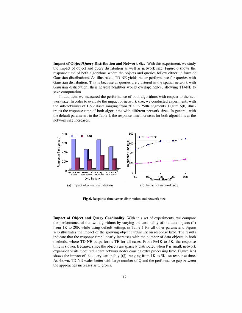
Impact of Object/Query Distribution and Network Size With this experiment, we studythe impact of object and query distribution as well as network size. Figure 6 shows theresponse time of both algorithms where the objects and queries follow either uniform orGaussian distributions. As illustrated, TD-NE yields better performance for queries withGaussian distribution. This is because as queries are clustered in the spatial network withGaussian distribution, their nearest neighbor would overlap; hence, allowing TD-NE tosave computation.

In addition, we measured the performance of both algorithms with respect to the net-work size. In order to evaluate the impact of network size, we conducted experiments withthe sub-networks of LA dataset ranging from 50K to 250K segments. Figure 6(b) illus-trates the response time of both algorithms with different network sizes. In general, withthe default parameters in the Table 1, the response time increases for both algorithms as thenetwork size increases.

(a) Impact of object distribution (b) Impact of network size

Fig. 6. Response time versus distribution and network size

Impact of Object and Query Cardinality With this set of experiments, we comparethe performance of the two algorithms by varying the cardinality of the data objects (P)from 1K to 20K while using default settings in Table 1 for all other parameters. Figure7(a) illustrates the impact of the growing object cardinality on response time. The resultsindicate that the response time linearly increases with the number of data objects in bothmethods, where TD-NE outperforms TE for all cases. From P=1K to 5K, the responsetime is slower. Because, since the objects are sparsely distributed when P is small, networkexpansion visits more redundant network nodes causing extra processing time. Figure 7(b)shows the impact of the query cardinality (Q), ranging from 1K to 5K, on response time.As shown, TD-NE scales better with large number of Q and the performance gap betweenthe approaches increases as Q grows.

12

(a) Impact of object cardinality (b) Impact of query cardinality

Fig. 7. Response time versus query/object cardinality and agility

6 Conclusion and Future Work

In this paper, for the first time we studied the problem of time-dependent k nearest neighborsearch (TD-kNN) in spatial networks. We formulated a generalized type of k nearest neigh-bor query where we, unlike the existing studies, assume the edge weights of the network aretime varying rather than fixed. We studied two baseline solutions exploiting time-expandednetwork and network expansion frameworks and compared their efficiency with real-worlddata-sets, including a variety of large spatial networks with real traffic-data. Although time-expanded network framework provides a mechanism to use existing kNN algorithms forstatic networks, the experimental results suggest that the error rate (incorrectly identifiednearest neighbors) of this approach is very high especially during traffic peak hours. Onthe other hand, while network expansion yields correct results at all times, the overhead ofexecuting network expansion is very high particularly in large networks with a sparse setof data objects, hence the need for efficient time-dependent search algorithms.

We intend to pursue this study in three different directions. First, we intend to inves-tigate new data models for effective representation of spatiotemporal road networks. Thisis critical in supporting development of efficient and accurate time-dependent algorithms(e.g., shortest path), while minimizing the storage and cost of the computation. Second,given that online nearest neighbor queries require near real-time response time, we plan todevelop novel preprocessing and indexing techniques that can be used to accelerate kNNcomputation in time-dependent networks. Third, we plan to study a variety of other spatialqueries (including range queries and skyline queries) in time-dependent road networks.

Given the importance of time-dependency for accurate and realistic spatial query pro-cessing in road networks, as well as increasing use of traffic sensors and, hence; availabilityof time-varying traffic data, we predict rapid growth of interest (at academia and industry)in developing various query processing solutions for spatial queries in time-dependent roadnetworks.

13

References

1. I. Chabini. The discrete-time dynamic shortest path problem: Complexity, algorithms, and im-plementations. In Transportation Research Record, 1999.

2. H.-J. Cho and C.-W. Chung. An efficient and scalable approach to cnn queries in a road network.In VLDB, 2005.

3. L. Cooke and E. Halsey. The shortest route through a network with timedependent internodaltransit times. In Journal of Mathematical Analysis and Applications, 1966.

4. B. C. Dean. Algorithms for minimum cost paths in time-dependent networks. In Networks, 1999.5. U. Demiryurek, F. Banaei-Kashani, and C. Shahabi. Efficient continuous nearest neighbor query

in spatial networks using euclidean restriction. In SSTD, 2009.6. U. Demiryurek, B. Pan, F. B. Kashani, and C. Shahabi. Towards modeling the traffic data on

road networks. In GIS-IWCTS, 2009.7. B. Ding, J. X. Yu, and L. Qin. Finding time-dependent shortest paths over large graphs. In

EDBT, 2008.8. S. E. Dreyfus. An appraisal of some shortest-path algorithms. In Operations Research Vol. 17,

No. 3, 1969.9. B. George, S. Kim, and S. Shekhar. Spatio-temporal network databases and routing algorithms:

A summary of results. In SSTD, 2007.10. A. Guttman. R-trees: A dynamic index structure for spatial searching. In SIGMOD, 1984.11. J. Halpern. Shortest route with time dependent length of edges and limited delay possibilities in

nodes. In Mathematical Methods of Operations Research, 1969.12. X. Huang, C. S. Jensen, and S. Saltenis. The island approach to nearest neighbor querying in

spatial networks. In SSTD, 2005.13. X. Huang, C. S. Jensen, and S. Saltenis. S-grid: A versatile approach to efficient query processing

in spatial networks. In SSTD, 2007.14. Inrix. http://www.inrix.com. Last visited January 2, 2010.15. E. Kanoulas, Y. Du, T. Xia, and D. Zhang. Finding fastest paths on a road network with speed

patterns. In ICDE, 2006.16. M. Kolahdouzan and C. Shahabi. Voronoi-based k nearest neighbor search for spatial network

databases. In VLDB, 2004.17. U. Lauther. An extremely fast, exact algorithm for finding shortest paths in static networks with

geographical background. In Geoinformation and Mobilitat, 2004.18. K. Mouratidis, M. L. Yiu, D. Papadias, and N. Mamoulis. Continuous nearest neighbor monitor-

ing in road networks. In VLDB, 2006.19. Navteq. http://www.navteq.com. Last visited January 2, 2010.20. A. Orda and R. Rom. Shortest-path and minimum-delay algorithms in networks with time-

dependent edge-length. J. ACM, 1990.21. S. Pallottino and M. G. Scutell. Shortest path algorithms in transportation models: Classical and

innovative aspects. In Equilibrium and Advanced Transportation Modelling, 1998.22. D. Papadias, J. Zhang, N. Mamoulis, and Y. Tao. Query processing in spatial network databases.

In VLDB, 2003.23. H. Samet, J. Sankaranarayanan, and H. Alborzi. Scalable network distance browsing in spatial

databases. In SIGMOD, 2008.24. D. Wagner and T. Willhalm. Geometric speed-up techniques for finding shortest paths in large

sparse graphs. Algorithms-ESA, 2003.

14