towards graph analytics and privacy protectionnew privacy concerns for the individuals involved. in...
TRANSCRIPT

Towards Graph Analytics and Privacy Protectionby
Dongqing Xiao
A Dissertation
Submitted to the Faculty
of the
WORCESTER POLYTECHNIC INSTITUTE
In partial fulfillment of the requirements for the
Degree of Doctor of Philosophy
in
Computer Science
by
APPROVED:
Professor Mohamed Y. EltabakhWorcester Polytechnic InstituteAdvisor
Professor Elke A. RundensteinerWorcester Polytechnic InstituteCommittee Member
Professor Craig WillsWorcester Polytechnic InstituteHead of Department
Professor Xiangnan KongWorcester Polytechnic InstituteCommittee Member
Dr. Yuanyuan TianIBM AlmadenExternal Committee Member

Abstract
In many prevalent application domains, such as business to business network,
social networks, and sensor networks, graphs serve as a powerful model to
capture the complex relationships inside. These graphs are of significant im-
portance in various domains such as marketing, psychology, and system de-
sign. The management and analysis of these graphs is a recurring research
theme. The increasing scale of data poses a new challenge on graph analysis
tasks. Meanwhile, the revealed edge uncertainty in the released graph raises
new privacy concerns for the individuals involved.
In this dissertation, we first study how to design an efficient distributed tri-
angle listing algorithms for web-scale graphs with MapReduce. This is a
challenging task since triangle listing requires accessing the neighbors of the
neighbor of a vertex, which may appear arbitrarily in different graph parti-
tions (poor locality in data access). We present the Bermuda method that
effectively reduces the size of the intermediate data via redundancy elimina-
tion and sharing of messages whenever possible. Bermuda encompasses two
general optimization principles that fully utilize the locality and re-use dis-
tance of local pivot message. Leveraging these two principles, Bermuda not
only speeds up the triangle listing computations by factors up to 10 times but
also scales up to larger datasets.
Second, we focus on designing anonymization approach to resisting de-anonymization
with little utility loss over uncertain graphs. In uncertain graphs, the adver-
sary can also take advantage of the additional information in the released
uncertain graph, such as the uncertainty of edge existence, to re-identify
the graph nodes. In this research, we first show the conventional graph
anonymization techniques either fails to guarantee anonymity or deteriorates
utility over uncertain graphs. To this end, we devise a novel and efficient
framework Chameleon that seamlessly integrates uncertainty. First, a proper
utility evaluation model for uncertain graphs is proposed. It focuses on the
changes on uncertain graph reliability features, but not purely on the amount
of injected noise. Second, an efficient algorithm is designed to anonymize
a given uncertain graph with relatively small utility loss as empowered by
reliability-oriented edge selection and anonymity-oriented edge perturbing.
Experiments confirm that at the same level of anonymity, Chameleon pro-
vides higher utility than the adaptive version of deterministic graph anonymiza-
tion methods.
Lastly, we consider resisting more complex re-identification risks and pro-
pose a simple-yet-effective Galaxy framework for anonymizing uncertain
graphs by strategically injecting edge uncertainty based on nodes role. In par-
ticular, the edge modifications are bounded by the derived anonymous proba-
bilistic degree sequence. Experiments show our method effectively generates
anonymized uncertain graphs with high utility.

Acknowledgements
The growth of my knowledge over the last few years is to a huge part due
to the inspiration and guidance I received from my advisor, Professor Prof.
Mohamed Eltabakh. He gave me the freedom to explore any topic in graph
analytics research, provided sound directions at every turn, and the prompt
feedback that pushed my research process. I have been fortunate to have him
as my advisor. I express my sincere thanks for his support, advice, patience,
and encouragement throughout my Ph.D career. I am grateful to Prof. Xi-
angnan Kong for always being patient and being there for our discussion.
I sincerely thank the members of my Ph.D. committee, Prof. Elke runden-
steiner, Professor Xiangnan Kong, and Dr. YuanYuan Tian for providing me
valuable feedback during all milestones in my Ph.D study. Their insightfull
suggestion helped me improve my research and the content of this disserta-
tion. I would like to thank Prof. Elke rundensteiner for her guidance for my
research qualification. My thanks also goes to the National Science Foun-
dation (NSF) for providing funding for the computing resources used in my
dissertation.
I would like to thank my collaborators Karim Ibrahim, Hai Liu and Pankaj
Didwania. My thank you also goes to all other previous and current DSRG
members – in particular Dr. Chuan Lei, Dr. Lei Cao, Yizhou Yan and Xiao
Qin for their insightful discussion, helpful feedback, and friendship.

I would like to thank my family members for their patience, support and love
during the past few years. Their passion to achieve bigger and better things
ingrained in me is a drive to reach excellence.

My Publications
Publications Contributing to this Dissertation
In this context I have achieved research advances that are selectively included in this
dissertation as detailed below.
Topic I:
Topic I of this dissertation addresses the problem of distributed triangle listing for massive
graphs.
1. Dongqing Xiao, Mohamed Y. Eltabakh, Xiangnan Kong, Bermuda: An Efficient
MapReduce Triangle Listing Algorithm for Web-Scale Graphs. SSDBM 2016,
pages 1-12.
Relationship to this dissertation: In this work, we propose “Bermuda” method that
effectively reduces the size of the intermediate data via redundancy elimination and
sharing of messages whenever possible, together for efficient triangle listing.
Chapters 2 to 5 in Part I of this dissertation are based on this work.
iii

Topic II: Degree Anonymization over Uncertain Graphs
Topic II of this dissertation addresses the problem of resisting degree-based de-anonymization
over anonymized uncertain graphs.
2. Dongqing Xiao, Mohamed Y. Eltabakh, Xiangnan Kong, Chameleon: Towards the
Preservation of Privacy and Reliability in Anonymized Uncertain Graphs, in sub-
mission to a major conference.
Relationship to this dissertation: In this work, we present Chameleon, the first
anonymization framework for uncertain graphs, namely, Chameleon. Chameleon
constructs the anonymized uncertain graphs in iterative skeleton empowered by (1)
an efficient cost-benfit oriented edge selection strategy to identify the candidate
edge sets for obfuscation (2) an efficient entropy-driven edge perturbation strategy
for maximizing the privacy gain.
Chapters 6 to 10 in Part II of this dissertation are based on this work.
Topic III: Probabilistic Degree Anonymization over Uncertain Graphs
Topic III of this dissertation address the novel probabilistic degree-based re-identification
problem over uncertain graphs.
3. Dongqing Xiao, Mohamed Y. Eltabakh, Xiangnan Kong, Galaxy: Resisting Proba-
bilistic Re-identification in Anonymized Uncertain Graphs ready for submission to
a major conference.
Relationship to dissertation: In this work, we present Galaxy framework which
leverages the (k, ε)-obf degree sequence to bound and guide the random perturbation-
based anonymization schemes.
Chapters 11 to 13 in Part II of this dissertation are based on this work.
iv

Other Publications
The below listed publications correspond to other research projects I have undertaken dur-
ing my PhD at WPI mostly on the topic of query optimization and meta data management.
4. Hai Liu, Dongqing Xiao, Pankaj Didwania, Mohamed Y. Eltabakh: Exploiting Soft
and Hard Correlations in Big Data Query Optimization. PVLDB 2016, pages 1005-
1016.
5. Karim Ibrahim, Dongqing Xiao, Mohamed Y. Eltabakh, Elevating Annotation Sum-
maries To First-Class Citizens In InsightNotes. EDBT 2015, pages 49-60.
6. Dongqing Xiao, Mohamed Y. Eltabakh: InsightNotes: summary-based annotation
management in relational databases.SIGMOD 2014, pages 661-672.
v
Contents
My Publications iii
List of Figures xi
List of Tables xiii
1 Introduction 1
1.1 Motivation . . . . . . . . . . . . . . . . . . . . . . . . . . . . . . . . . . 1
1.1.1 Distributed Triangle Listing for Massive Graphs . . . . . . . . . 1
1.1.2 Uncertain Graph Anonymization . . . . . . . . . . . . . . . . . . 3
1.2 State-Of-the-Art . . . . . . . . . . . . . . . . . . . . . . . . . . . . . . . 5
1.2.1 Distributed Triangle Listing Algorithms . . . . . . . . . . . . . . 5
1.2.2 Determinitic Graph Anonymization . . . . . . . . . . . . . . . . 7
1.3 Research Challenges Addressed in This Dissertation . . . . . . . . . . . 13
1.4 Proposed Solutions . . . . . . . . . . . . . . . . . . . . . . . . . . . . . 15
1.4.1 Distributed Triangle Listing . . . . . . . . . . . . . . . . . . . . 16
1.4.2 Resisting Degree-based De-anonymization in Uncertain Graphs . 17
1.4.3 Resisting Probabilistic Degree-based De-anonymization in Un-
certain Graphs . . . . . . . . . . . . . . . . . . . . . . . . . . . 19
1.5 Dissertation Organization . . . . . . . . . . . . . . . . . . . . . . . . . . 20
vi

CONTENTS
I Distributed Triangle Listing With MapReduce 22
2 Bermuda Preliminaries 23
2.1 Triangle Listing Problem . . . . . . . . . . . . . . . . . . . . . . . . . . 23
2.2 Sequential Triangle Listing . . . . . . . . . . . . . . . . . . . . . . . . . 24
2.3 MapReduce Overview . . . . . . . . . . . . . . . . . . . . . . . . . . . 26
2.4 Triangle Listing in MapReduce . . . . . . . . . . . . . . . . . . . . . . . 27
2.4.1 Analysis and Optimization Opportunities . . . . . . . . . . . . . 28
3 Bermuda Technique 31
3.1 Bermuda Edge-Centric Node++ . . . . . . . . . . . . . . . . . . . . . . 32
3.1.1 Analysis of Bermuda-EC . . . . . . . . . . . . . . . . . . . . . . 34
3.2 Bermuda Vertex-Centric Node++ . . . . . . . . . . . . . . . . . . . . . . 38
3.2.1 Message Sharing Management . . . . . . . . . . . . . . . . . . . 41
3.2.1.1 Usage-Based Tracking . . . . . . . . . . . . . . . . . . 42
3.2.1.2 Bucket-Based Tracking . . . . . . . . . . . . . . . . . 43
3.2.2 Analysis of Bermuda-VC . . . . . . . . . . . . . . . . . . . . . . 44
4 Performance Evaluation 46
4.1 Datasets . . . . . . . . . . . . . . . . . . . . . . . . . . . . . . . . . . . 47
4.2 Experiment Result . . . . . . . . . . . . . . . . . . . . . . . . . . . . . 47
4.2.1 Bermuda Technique . . . . . . . . . . . . . . . . . . . . . . . . 48
4.2.2 Effect of the number of reducers . . . . . . . . . . . . . . . . . . 49
4.2.3 Message Sharing Management . . . . . . . . . . . . . . . . . . . 51
4.2.4 Execution Time Performance . . . . . . . . . . . . . . . . . . . . 52
5 Related Works 54
vii
CONTENTS
II Resisting Degree-based De-anonymization in Anonymized Un-
certain Graphs 57
6 Problem Definition 58
6.1 Uncertain Graph . . . . . . . . . . . . . . . . . . . . . . . . . . . . . . . 58
6.2 Attack Model and Privacy Criteria . . . . . . . . . . . . . . . . . . . . . 59
6.3 Reliability-Based Utility Loss Metric . . . . . . . . . . . . . . . . . . . . 60
6.4 Problem Statement . . . . . . . . . . . . . . . . . . . . . . . . . . . . . 61
7 Uncertain Graph Anonymization via Representative Instance 62
8 Chameleon Framework 64
8.1 Chameleon Iterative Skeleton . . . . . . . . . . . . . . . . . . . . . . . . 64
8.2 Hybrid Edge Selection . . . . . . . . . . . . . . . . . . . . . . . . . . . 66
8.2.1 Uniqueness Score . . . . . . . . . . . . . . . . . . . . . . . . . . 67
8.2.2 Reliability Relevance . . . . . . . . . . . . . . . . . . . . . . . . 68
8.3 Reliability-oriented Edge Selection Procedure . . . . . . . . . . . . . . . 73
8.4 Anonymity-Oriented Edge Perturbing . . . . . . . . . . . . . . . . . . . 76
9 Performance Evaluation 83
9.1 Experiment Settings . . . . . . . . . . . . . . . . . . . . . . . . . . . . . 83
9.1.1 Data Collection . . . . . . . . . . . . . . . . . . . . . . . . . . . 83
9.1.2 Evaluation Metrics . . . . . . . . . . . . . . . . . . . . . . . . . 85
9.2 Performance of Uncertain Graph Anonymization . . . . . . . . . . . . . 87
9.2.1 Efficiency Evaluation . . . . . . . . . . . . . . . . . . . . . . . . 87
9.2.2 Utility Loss . . . . . . . . . . . . . . . . . . . . . . . . . . . . . 88
10 Related Work 92
viii
CONTENTS
III Resisting Probabilistic Degree-based De-anonymization in Anonymized
Uncertain Graphs 96
11 Problem Definition 97
11.1 Privacy Threats . . . . . . . . . . . . . . . . . . . . . . . . . . . . . . . 97
11.2 Anonymity Measurement . . . . . . . . . . . . . . . . . . . . . . . . . . 100
11.3 Utility Preservation . . . . . . . . . . . . . . . . . . . . . . . . . . . . . 101
11.4 Problem Statement . . . . . . . . . . . . . . . . . . . . . . . . . . . . . 101
12 Galaxy Techniques 104
12.1 Overview of The Galaxy Approach . . . . . . . . . . . . . . . . . . . . . 104
12.2 Probabilistic Degree Anonymization . . . . . . . . . . . . . . . . . . . . 107
12.3 Probabilistic Degree Sequence Alignment . . . . . . . . . . . . . . . . . 110
12.4 Probablistic Anonymous Graph Construction . . . . . . . . . . . . . . . 112
12.5 The Anonymity-Bounded Obfuscation Algorithm . . . . . . . . . . . . . 113
13 Performance Evaluation 117
13.1 Experiment Settings . . . . . . . . . . . . . . . . . . . . . . . . . . . . . 117
13.1.1 Data Collection . . . . . . . . . . . . . . . . . . . . . . . . . . . 117
13.1.2 Utility Evaluation . . . . . . . . . . . . . . . . . . . . . . . . . . 118
13.2 Performance of Uncertain Graph Anonymization . . . . . . . . . . . . . 119
13.2.1 Efficiency Evaluation . . . . . . . . . . . . . . . . . . . . . . . . 119
13.2.2 Utility Loss Evaluation . . . . . . . . . . . . . . . . . . . . . . . 121
IV Conclusion and Future Work 124
14 Conclusion of This Dissertation 125
ix

CONTENTS
15 Future Work 127
15.1 Defeating More Involved De-anonymization Attacks . . . . . . . . . . . 127
15.2 Big Graph Anonymization . . . . . . . . . . . . . . . . . . . . . . . . . 129
15.3 Learning to Anonymize Uncertain Graphs . . . . . . . . . . . . . . . . . 130
References 133
x

List of Figures
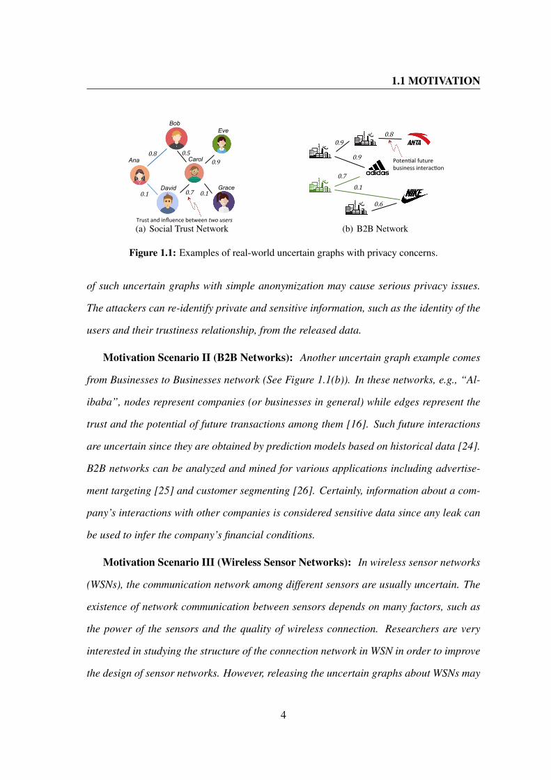
1.1 Examples of real-world uncertain graphs with privacy concerns. . . . . . 4
2.1 Bermuda: Adjacency List. . . . . . . . . . . . . . . . . . . . . . . . . . 23
3.1 Bermuda: Bermuda-EC (Edge Centric) Execution. . . . . . . . . . . . . 34
3.2 Bermuda: Bermuda-VC (Vertex Centric) Execution. . . . . . . . . . . . . 39
3.3 Bermuda: Access Patterns of Pivot Messages. . . . . . . . . . . . . . . . 42
3.4 Bermuda: The Usage of External Memory. . . . . . . . . . . . . . . . . . 43
4.1 Bermuda: Distribution of Mapper Elapsed Times. . . . . . . . . . . . . . 48
4.2 Bermuda: Disk Space vs. Memory Tradeoff. . . . . . . . . . . . . . . . . 49
4.3 Bermuda: Running Time of Bermuda-EC. . . . . . . . . . . . . . . . . . 49
4.4 Bermuda (disk-based): Varying k vs. Running Time. . . . . . . . . . . . 51
4.5 Bermuda: The Accumulation of Sharing Messages. . . . . . . . . . . . . 51
6.1 Chameleon: Privacy Risk Assessment. . . . . . . . . . . . . . . . . . . . 59
7.1 Chameleon: Representative based Anonymization (Rep-An). . . . . . . . 63
8.1 Chameleon: Edge Modifications’ Impact vs. Relaiblity Relevance. . . . . 70
8.2 Chameleon: Sampling Estimator for ERR . . . . . . . . . . . . . . . . . 72
8.3 Chameleon: Anonymity-Oriented Edge Perturbation. . . . . . . . . . . . 77
xi

LIST OF FIGURES
9.1 Chameleon: Distribution of Edge Probabilities, Degrees. . . . . . . . . . 84
9.2 Chameleon: Two Terminal Reliablity Discrepancy. . . . . . . . . . . . . 86
9.3 Chameleon: Running Time Comparision vs. Rep-An. . . . . . . . . . . . 87
9.4 Chameleon: Graph Property Preservation. . . . . . . . . . . . . . . . . . 88
9.5 Chameleon: Double Loss of Rep-An. . . . . . . . . . . . . . . . . . . . 89
9.6 Chameleon: The Gain of RS and ME. . . . . . . . . . . . . . . . . . . . 90
11.1 Galaxy: Probabilistic Degree-based De-anonymization. . . . . . . . . . . 99
11.2 Galaxy: Illustration of Convex and Non-Convex Set. . . . . . . . . . . . 102
11.3 Galaxy: Invalidity of Being Convex Set. . . . . . . . . . . . . . . . . . . 103
12.1 Galaxy Framework. . . . . . . . . . . . . . . . . . . . . . . . . . . . . . 105
12.2 Galaxy: Probabilistic Degree Sequence Approximation. . . . . . . . . . . 108
12.3 Galaxy: Fuzzy Vertex Alignments. . . . . . . . . . . . . . . . . . . . . . 110
12.4 Galaxy: Derived Perturbation Model. . . . . . . . . . . . . . . . . . . . 112
12.5 Galaxy: Anonymous Degree Sequence Realization. . . . . . . . . . . . . 114
13.1 Galaxy: Running Time Comparisions vs. Chameleon. . . . . . . . . . . . 120
13.2 Galaxy: Two Terminal Reliablity Preservation. . . . . . . . . . . . . . . 120
13.3 Galaxy: The Change Ratio of Degree. . . . . . . . . . . . . . . . . . . . 121
13.4 Galaxy: Average Path Distance Preservation. . . . . . . . . . . . . . . . 122
13.5 Galaxy: Clustering Coefficient Preservation. . . . . . . . . . . . . . . . . 122
13.6 Galaxy: Degree Distribution Preservation. . . . . . . . . . . . . . . . . . 123
15.1 Parallel Graph Anonymization Process. . . . . . . . . . . . . . . . . . . 130
15.2 Graph Anonymization Learning Process. . . . . . . . . . . . . . . . . . . 131
xii
List of Tables
2.1 Bermuda:Summary of Notations. . . . . . . . . . . . . . . . . . . . . . . 24
4.1 Bermuda: Basic Statistics about Datasets. . . . . . . . . . . . . . . . . . 47
4.2 Bermuda: Reduction Factors of Communication Cost. . . . . . . . . . . . 47
4.3 Bermuda: Effectiveness Evaluation. . . . . . . . . . . . . . . . . . . . . 52
9.1 Chameleon: Dataset Statistics and Privacy Parameters. . . . . . . . . . . 84
9.2 Chameleon: Summary of Uncertain Graph Anonymization Methods. . . . 86
10.1 Chameleon: Summary of Adversary Knowledge. . . . . . . . . . . . . . 93
10.2 Chameleon: Privacy Criteria Summary of Perturbation-based Graph Anonymiza-
tion Schemes. . . . . . . . . . . . . . . . . . . . . . . . . . . . . . . . . 93
10.3 Chameleon: Positioning Chameleon w.r.t State-Of-Art Techniques. . . . . 94
13.1 Galaxy: Dataset Statistics and Privacy Parameters. . . . . . . . . . . . . . 118
xiii

1
Introduction
1.1 Motivation
1.1.1 Distributed Triangle Listing for Massive Graphs
Graphs arise naturally in many real-world applications such as social networks, bio-
medical networks, and communication networks. In these applications, the graph can
often be massive involving billions of vertices and edges. For example, Facebook’s social
network involves more than 1.23 billion users (vertices), and more than 208 billion friend-
ships (edges). Such massive graphs can easily exceed the available memory of a single
commodity computer. That is why distributed analysis on massive graphs has become an
important research area in recent years [1, 2].
Triangle listing—which involves listing all triangles in a given graph—is well identi-
fied as a building-block operation in many graph analysis and mining techniques [3, 4].
First, several graph metrics can be directly obtained from triangle listing, e.g., clustering
coefficient and transitivity. Such graph metrics have wide applications including quantify-
ing graph density, detecting spam pages in web graphs, and measuring content quality in
social networks [5]. Moreover, triangle listing has a broad range of applications including
1
1.1 MOTIVATION
the discovery of dense sub-graphs [4], study of motif occurrences [6], and uncovering of
hidden thematic relations in the web [3]. There is another well-known and closely-related
problem to triangle listing, which is the triangle counting problem. Clearly, solving the
triangle listing problem would automatically solve triangle counting, but not vice versa.
Compared to triangle counting, triangle listing serves a broader range of applications. For
example, Motif identification [6], community detection [7], and dense subgraphs [4] are
all dependent on the more complex triangle listing problem.
Several techniques have been proposed for processing web-scale graphs including
streaming algorithms [5, 8], external-memory algorithms [9, 10, 11], and distributed
parallel algorithms [12, 13]. The streaming algorithms are limited to the approximate
triangle counting problem. External-memory algorithms exploit asynchronous I/O and
multi-core parallelism for efficient triangle listing [9, 11, 14]. In spite of achieving an
impressive performance, external-memory approaches assume that the input graphs are
in a centralized storage, which is not the case for many emerging applications that gen-
erate graphs distributed in nature. Even more seriously, external-memory approaches
cannot easily scale up in terms of computing resources and parallelization degree. Algo-
rithm [13] presents a parallel algorithm for exact triangle counting using the MapReduce
framework. The algorithm proposes a partitioning scheme that improves the memory re-
quirements to some extent, yet it still suffers from a huge communication cost. Algorithm
[12] presents an efficient MPI-based distributed memory algorithm on the basis of [13]
with load balancing techniques. However, as a memory-based algorithm, it suffers from
memory limitations.
In addition to these techniques, several distributed and specialized graph frameworks
have been recently proposed as general-purpose graph processing engines [1, 2, 15].
However, most of these frameworks are customized for iterative graph processing where
distributed computations can be kept in-memory for faster subsequent iterations. How-
2
1.1 MOTIVATION
ever, the triangle listing algorithms are not iterative and would not make use of these
optimizations.
1.1.2 Uncertain Graph Anonymization
In many prevalent application domains, such as business to business (B2B) [16], social
networks [17, 18], and sensor networks [19], graphs serve as powerful models to capture
the complex relationships inherent in these applications. Most graphs in these applications
are uncertain by nature, where each edge carries a degree of uncertainty (probability)
representing the probability of its presence in the real world. This uncertainty can be due
to various reasons ranging from the use of prediction models to predict the edges (as in
social media and B2B networks) to physical properties that affect the edges’ reliabilities
(as in sensor and communication networks).
These rich uncertain graphs are of significant importance due to the analytics and
knowledge extraction that can be applied on them, e.g., understanding graph structures [20,
21], social interactions [22], information discovery and propagation [23], advertising and
marketing [18], among many others. Publishing such uncertain graph data would allow
a wide variety of ad hoc analyses and novel valid uses of the data, but it also raises huge
privacy concerns. This is because these uncertain graphs contain sensitive information
about the graph entities as well as their connections, whose disclosure may violate pri-
vacy regulations.
Motivation Scenario I (Social Trust Networks): In social networks, the trust and
influence relationships among users—which may greatly impact users’ behaviors—are
usually probabilistic and uncertain [18] (See Figure 1.1(a)). The existence of the trust re-
lationship depends on many factors, such as the area of expertise and emotional connec-
tions. Researchers are very interested in studying the structure of social trust networks,
in order to promote products, or choose strategies for a campaign. However, the release
3
1.1 MOTIVATION
Ana
Bob
Carol
David
Eve
Grace
0.8
0.1 0.7
0.5 0.9
0.1
0.7 0.1
0.9
0.9 0.8
Trustandinfluencebetweentwousers
Potennalfuturebusinessinteracnon
0.6
(a) Social Trust Network
Ana
Bob
Carol
David
Eve
Grace
0.8
0.1 0.7
0.5 0.9
0.1
0.7 0.1
0.9
0.9 0.8
Trustandinfluencebetweentwousers
Potennalfuturebusinessinteracnon
0.6
(b) B2B Network
Figure 1.1: Examples of real-world uncertain graphs with privacy concerns.
of such uncertain graphs with simple anonymization may cause serious privacy issues.
The attackers can re-identify private and sensitive information, such as the identity of the
users and their trustiness relationship, from the released data.
Motivation Scenario II (B2B Networks): Another uncertain graph example comes
from Businesses to Businesses network (See Figure 1.1(b)). In these networks, e.g., “Al-
ibaba”, nodes represent companies (or businesses in general) while edges represent the
trust and the potential of future transactions among them [16]. Such future interactions
are uncertain since they are obtained by prediction models based on historical data [24].
B2B networks can be analyzed and mined for various applications including advertise-
ment targeting [25] and customer segmenting [26]. Certainly, information about a com-
pany’s interactions with other companies is considered sensitive data since any leak can
be used to infer the company’s financial conditions.
Motivation Scenario III (Wireless Sensor Networks): In wireless sensor networks
(WSNs), the communication network among different sensors are usually uncertain. The
existence of network communication between sensors depends on many factors, such as
the power of the sensors and the quality of wireless connection. Researchers are very
interested in studying the structure of the connection network in WSN in order to improve
the design of sensor networks. However, releasing the uncertain graphs about WSNs may
4

1.2 STATE-OF-THE-ART
cause privacy or security problems. For example, the WSNs in smart power grids are of
great value in research studies, but the release of such data can potentially cause attacks
to the power grid system, especially if attackers can re-identify the exact locations of the
sensors from the released data.
These scenarios show the immediate need for efficient uncertain graph anonymization,
i.e., protecting the sensitive information while maintaining the graph utility. In general,
the graph anonymization problem has been studied extensively and various anonymiza-
tion techniques have been proposed [27, 28, 29, 30, 31, 32, 33, 34]. However, these
techniques focus only on deterministic graphs, where edges’ presence is known with cer-
tainty.
1.2 State-Of-the-Art
1.2.1 Distributed Triangle Listing Algorithms
Triangle listing is a basic operation of the graph analysis. Many research works have been
conducted on this problem, which can be classified into three categories: in-memory algo-
rithms, external-memory algorithms and distributed algorithms. Here, we briefly review
these works.
In-Memory Algorithm. The majority of previously introduced triangle listing al-
gorithms are the In-Memory processing approaches. Traditionally, they can be further
classified as Node-Iterator[35, 36, 37] and Edge-Iterator ones[38, 39] with the respect to
iterator-type. Authors [37, 38, 39]improved the performance of in-memory algorithms
by adopting degree-based ordering. Matrix multiplication is used to count triangles [35].
However, all these algorithms are inapplicable to massive graphs which do not fit in mem-
ory.
5

1.2 STATE-OF-THE-ART
External-Memory Algorithms. In order to handle the massive graph, several external-
memory approaches were introduced [9, 10, 11]. Common idea of these methods is:
(1) Partition the input graph to make each partition fit into main-memory, (2) Load each
partition individually into main-memory and identify all its triangles, and then remove
edges which participated in the identified triangle, and (3) After the whole graph is loaded
into memory buffer once, the remaining edges are merged, then repeat former steps until
no edges remain. These Algorithms require a lot of disk I/Os to perform the reading and
writing of the edges. Authors [9, 10] improved the performance by reducing the amount
of disk I/Os and exploiting multi-core parallelism. External-Memory Algorithms show
great performance in time and space. However, the parallelization of external-memory
algorithms is limited. External-memory approaches cannot easily scale up in terms of
computing resources and parallelization degree.
Distributed Algorithms. Another promising approach to handle triangle listing on
large-scale graphs is the distributed computing. Suri et al. [13] introduced two Map-
Reduce adaptions of NodeIterator algorithm and the well-known Graph Partitioning (GP)
algorithm to count triangles. The Graph Partitioning algorithm utilizes one universal hash
partition function over nodes to distribute edges into overlapped graph partitions, then
identifies triangles over all the partitions. Park et al. [40] further generalized Graph Par-
titioning algorithm into multiple rounds, significantly increasing the size of the graphs
that can be handled on a given system. The authors compare their algorithm with GP
algorithm [13] across various massive graphs then show that they get speedups rang-
ing from 2 to 5. In this work, we show such large or even larger speedup (from 5 to
10) can also be obtained by reducing the size intermediate result directly via our meth-
ods. Teixeira et al. [41] presented Arabesque, one distributed data processing platform
for implementing subgraph mining algorithms on the basis of MapReduce framework.
Arabesque automates the process of exploring a very large number of subgraphs, includ-
6
1.2 STATE-OF-THE-ART
ing triangles. However, these MapReduce algorithms must generate a large amount of
intermediate data that travel over the network during the shuffle operation, which degrade
their performance. Arifuzzaman et al. [12] introduced an efficient MPI-based distributed
memory parallel algorithm (Patric) on the basis of NodeIterator algorithm. The Patric al-
gorithm introduced degree-based sorting preprocessing step for efficient set intersection
operation to speed up execution. Furthermore, several distributed solutions designed for
subgraph mining on large graph were also proposed [1, 42]. Shao et al. introduced the
PSgl framework to iteratively enumerate subgraph instance. Different from other parallel
approaches, the PSgl framework completes relies on the graph traversal and avoids the
explicit join operation. These distributed memory parallel algorithms achieve impressive
performance over large-scale graph mining tasks. These methods distributed the data
graph among the worker’s memory, thus they are not suitable for processing large-scale
graph with small clusters.
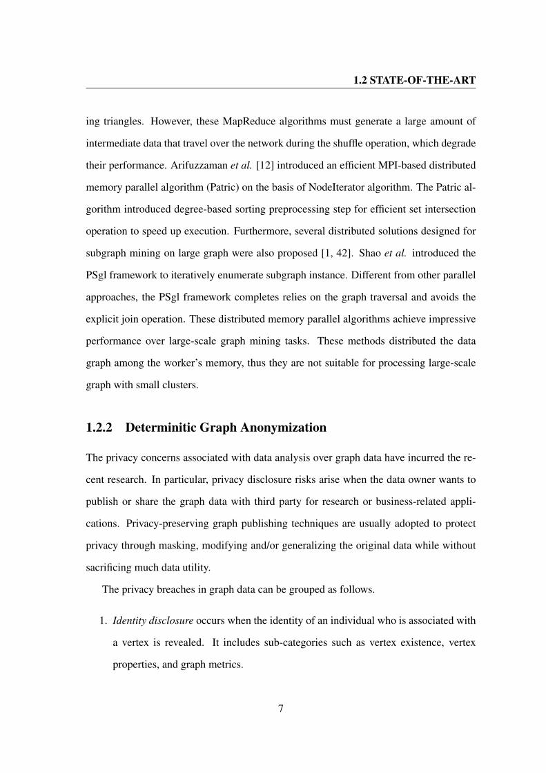
1.2.2 Determinitic Graph Anonymization
The privacy concerns associated with data analysis over graph data have incurred the re-
cent research. In particular, privacy disclosure risks arise when the data owner wants to
publish or share the graph data with third party for research or business-related appli-
cations. Privacy-preserving graph publishing techniques are usually adopted to protect
privacy through masking, modifying and/or generalizing the original data while without
sacrificing much data utility.
The privacy breaches in graph data can be grouped as follows.
1. Identity disclosure occurs when the identity of an individual who is associated with
a vertex is revealed. It includes sub-categories such as vertex existence, vertex
properties, and graph metrics.
7
1.2 STATE-OF-THE-ART
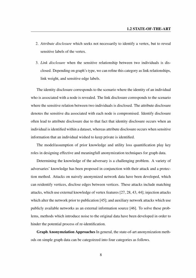
2. Attribute disclosure which seeks not necessarily to identify a vertex, but to reveal
sensitive labels of the vertex.
3. Link disclosure when the sensitive relationship between two individuals is dis-
closed. Depending on graph’s type, we can refine this category as link relationships,
link weight, and sensitive edge labels.
The identity disclosure corresponds to the scenario where the identity of an individual
who is associated with a node is revealed. The link disclosure corresponds to the scenario
where the sensitive relation between two individuals is disclosed. The attribute disclosure
denotes the sensitive dta associated with each node is compromised. Identify disclosure
often lead to attribute disclosure due to that fact that identity disclosure occurs when an
individual is identified within a dataset, whereas attribute disclosure occurs when sensitive
information that an individual wished to keep private is identified.
The model/assumption of prior knowledge and utility loss quantification play key
roles in designing effective and meaningfull anonymization techniques for graph data.
Determining the knowledge of the adversary is a challenging problem. A variety of
adversaries’ knowledge has been proposed in conjunction with their attack and a protec-
tion method. Attacks on naively anonymized network data have been developed, which
can reidentify vertices, disclose edges between vertices. These attacks include matching
attacks, which use external knowledge of vertex features [27, 28, 43, 44]; injection attacks
which alter the network prior to publication [45]; and auxiliary network attacks which use
publicly available networks as an external information source [46]. To solve these prob-
lems, methods which introduce noise to the original data have been developed in order to
hinder the potential process of re-identification.
Graph Anonymziation Approaches In general, the state-of-art anonymization meth-
ods on simple graph data can be categoirzed into four categories as follows.
8

1.2 STATE-OF-THE-ART
• Generalization or clustering-based approaches which can be essentially regarded
as grouping vertices and edges into partitions called super-vertices and super-edges.
The details about individuals can be hidden properly, but the graph may be shrunk
considerably after anonymization, which may not be desirable for analyzing local
structures.
• Edge and vertex modification approaches first transform the data by edges or ver-
tices modification (adding and/or deleting) and then release the perturbed data. The
data is thus made available for unconstrained analysis with existing graph mining
techniques.
• Uncertain graphs are approaches based on adding or removing edges “partially” by
assigning a probability to each edge in the anonymous network. Instead of creating
or deleting edges, the set of all possible edges is considered and a probability is
assigned to each edge.
All mentioned methods first transform the data into different types of graph’s modi-
fications and then release the perturbed data. The data is thus made available for uncon-
strained analysis. On the contrary, there is “privacy preserving graph mining” methods,
which do not release data, but only the output of an analysis task. For instance, differential
privacy [47] is a well-known privacy preserving graph mining method. In our work, we
do not consider such method for anonymizing uncertain graphs, since they do not allow
us to release the entire network which allows ad-hoc graph analysis tasks.
• Generalization approaches
Generalization approaches can be essentially regarded as grouping vertices and edges into
partitions called super-vertices and super-edges. The details about individuals can be hid-
den properly, but the graph may be shrunk considerably after anonymization, which may
be not desirable for analyzing local structures. All methods developed, therefore, need the
9

1.2 STATE-OF-THE-ART
whole graph to be applied to. Consequently, they are not able to deal with the streaming
graph data. Here, we remind the reader new methods can be developed using this core
idea to generate anonymous graph dataset. The first approach of this category was pro-
posed by Hay et al. [48]. It uses the size of the partition to ensure node anonymity. After
grouping, each super-vertex represents at least k nodes and each super-edge represents
all the nodes between nodes in two super-vertices. Only the edge density is published for
each partition, so it will be hard to distinguish between individuals in a partition. A sim-
ilar idea was applied for the complex network, i.e., labeled network [49].The clustering
problem is known to be NP-hard. Researchers ever present different methods for opti-
mization. For instance, Sihag et al. chose the genetic algorithm to optimize this NP-hard
problem. It does achieve a better result in terms of information loss. Unfortunately, this
method does not seem scalable for large networks.
• Edge and vertex modification approaches
Edge and vertex modification approaches anonymize a graph by modifying edges or ver-
tices in the graph. These modifications can be made at random (referred to as randomiza-
tion, random perturbation). random perturbation techniques are generally the simplest
and present the lowest complexity. Thus, they are able to deal with large networks. The
first method was proposed by Hay et al., called Random perturbation which anonymizes
unlabelled graphs using Rand add/del strategy, i.e., randomly removing p edges and then
randomly add p fake edges without change the set of vertices and the total number of
edges. On this basis, Ying and Wu [32, 50] developed two algorithms designed to pre-
serve spectral characteristics of the original graph called Spctr Add/Del and Spctr Switch.
Following the path, Stokes and Torra states an appropriate selection of the eigenvalues
in the spectral method can perturbation the graph while keeping its most significative
edges. The generic strategy which aims to preserve the most important edges in the net-
work trying to maximize utility while achieving the desired privacy level. Generally, such
10
1.2 STATE-OF-THE-ART
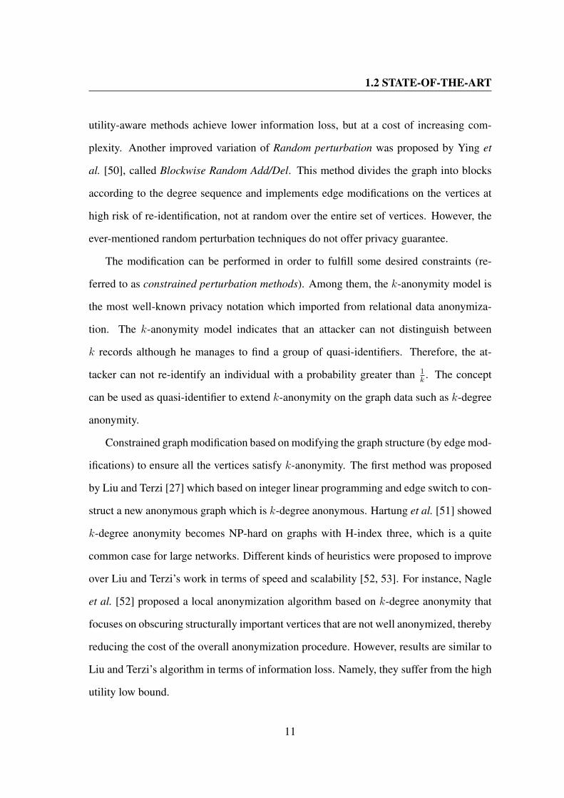
utility-aware methods achieve lower information loss, but at a cost of increasing com-
plexity. Another improved variation of Random perturbation was proposed by Ying et
al. [50], called Blockwise Random Add/Del. This method divides the graph into blocks
according to the degree sequence and implements edge modifications on the vertices at
high risk of re-identification, not at random over the entire set of vertices. However, the
ever-mentioned random perturbation techniques do not offer privacy guarantee.
The modification can be performed in order to fulfill some desired constraints (re-
ferred to as constrained perturbation methods). Among them, the k-anonymity model is
the most well-known privacy notation which imported from relational data anonymiza-
tion. The k-anonymity model indicates that an attacker can not distinguish between
k records although he manages to find a group of quasi-identifiers. Therefore, the at-
tacker can not re-identify an individual with a probability greater than 1k. The concept
can be used as quasi-identifier to extend k-anonymity on the graph data such as k-degree
anonymity.
Constrained graph modification based on modifying the graph structure (by edge mod-
ifications) to ensure all the vertices satisfy k-anonymity. The first method was proposed
by Liu and Terzi [27] which based on integer linear programming and edge switch to con-
struct a new anonymous graph which is k-degree anonymous. Hartung et al. [51] showed
k-degree anonymity becomes NP-hard on graphs with H-index three, which is a quite
common case for large networks. Different kinds of heuristics were proposed to improve
over Liu and Terzi’s work in terms of speed and scalability [52, 53]. For instance, Nagle
et al. [52] proposed a local anonymization algorithm based on k-degree anonymity that
focuses on obscuring structurally important vertices that are not well anonymized, thereby
reducing the cost of the overall anonymization procedure. However, results are similar to
Liu and Terzi’s algorithm in terms of information loss. Namely, they suffer from the high
utility low bound.
11
1.2 STATE-OF-THE-ART
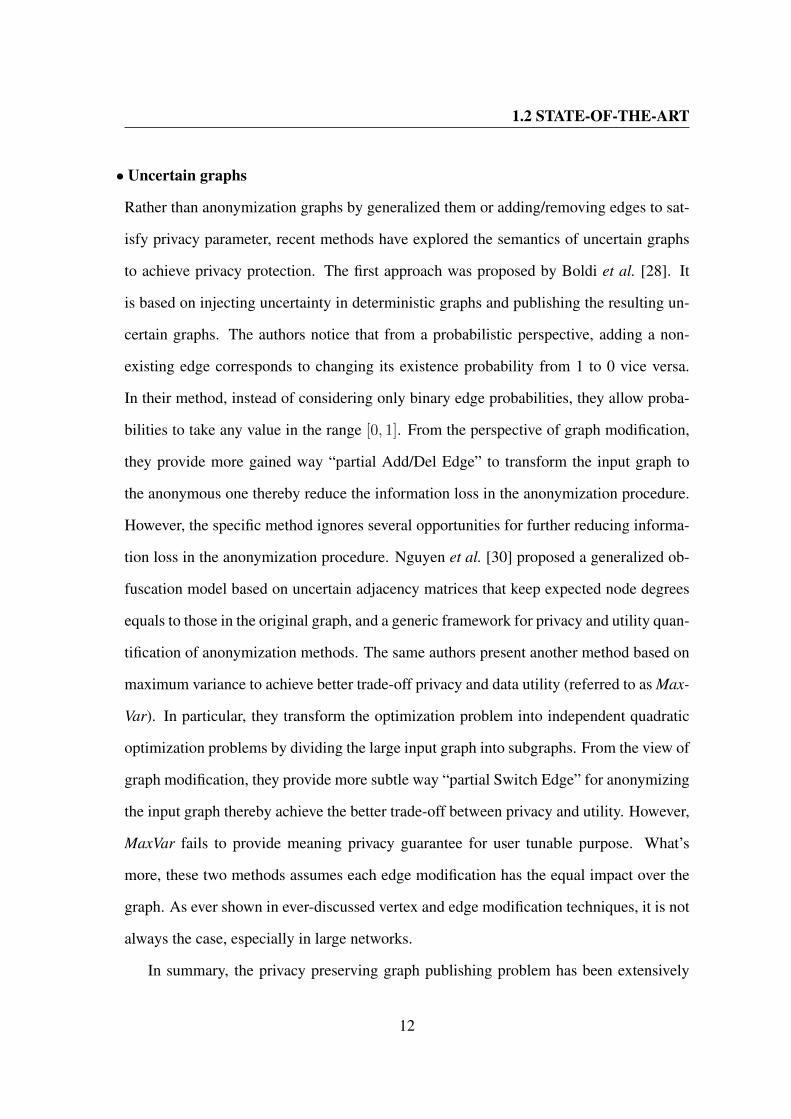
• Uncertain graphs
Rather than anonymization graphs by generalized them or adding/removing edges to sat-
isfy privacy parameter, recent methods have explored the semantics of uncertain graphs
to achieve privacy protection. The first approach was proposed by Boldi et al. [28]. It
is based on injecting uncertainty in deterministic graphs and publishing the resulting un-
certain graphs. The authors notice that from a probabilistic perspective, adding a non-
existing edge corresponds to changing its existence probability from 1 to 0 vice versa.
In their method, instead of considering only binary edge probabilities, they allow proba-
bilities to take any value in the range [0, 1]. From the perspective of graph modification,
they provide more gained way “partial Add/Del Edge” to transform the input graph to
the anonymous one thereby reduce the information loss in the anonymization procedure.
However, the specific method ignores several opportunities for further reducing informa-
tion loss in the anonymization procedure. Nguyen et al. [30] proposed a generalized ob-
fuscation model based on uncertain adjacency matrices that keep expected node degrees
equals to those in the original graph, and a generic framework for privacy and utility quan-
tification of anonymization methods. The same authors present another method based on
maximum variance to achieve better trade-off privacy and data utility (referred to as Max-
Var). In particular, they transform the optimization problem into independent quadratic
optimization problems by dividing the large input graph into subgraphs. From the view of
graph modification, they provide more subtle way “partial Switch Edge” for anonymizing
the input graph thereby achieve the better trade-off between privacy and utility. However,
MaxVar fails to provide meaning privacy guarantee for user tunable purpose. What’s
more, these two methods assumes each edge modification has the equal impact over the
graph. As ever shown in ever-discussed vertex and edge modification techniques, it is not
always the case, especially in large networks.
In summary, the privacy preserving graph publishing problem has been extensively
12
1.3 RESEARCH CHALLENGES ADDRESSED IN THIS DISSERTATION
studied, a lot of graph anonymization techniques have been proposed. However, they are
tailored towards determinitic graphs. The ignorance of edge uncertainty in anonymity and
utility loss assessment makes they neither provide enough anonymity nor preserve graph
utility in a right way.
1.3 Research Challenges Addressed in This Dissertation
Although many effective graph anonymization techniques have been proposed for de-
terministic graphs, shifting the graph anonymization techniques to uncertain graphs is
challenging.
It is challenging to develop a proper metric for quantifying the information loss for
uncertain graph anonymization. Fundamentally, the graph anonymization techniques re-
quired modifying graph structure at some level. The intermediate goal of graph anonymiza-
tion is to balance the utility and privacy. The first question we need to solve is to develop
proper metrics for quantifying loss of information. In the context of deterministic graphs,
this problem has been extensively studied. Most of the previous works use the total num-
ber of modified edges to measure the utility loss [27, 28]. Researchers argued this measure
is not effective as it assumes each edge modification has an equal impact on the original
graph properties [54]. They suggest studying the change on other structural properties
such as the spectrum [32], community structure [54], shortest path length and the neigh-
borhood overlap [33]. However, above-mentioned metrics are all designed for comparing
deterministic graphs and can not be used to handle uncertain graphs directly. Thus, we
need to investigate other utility metrics suitable for uncertain graphs which are able to
capture the essence of structural properties for better serving a wide range of analytics.
Developing metrics for quantifying loss of information for uncertain graph mining task is
a challenging research work on its own.
13

1.3 RESEARCH CHALLENGES ADDRESSED IN THIS DISSERTATION
It is challenging to define the adversary knowledge and privacy protection model
which explicitly incorporates edge uncertainty. Compared to deterministic graphs, the
publishing of uncertain graphs reveals additional information–associated edge uncertain-
ties which can be used by the adversary to re-identify some entities in the released uncer-
tain graph. Clearly, the public available edge uncertainty can be used to enhance various
kinds of de-anonymization attack. The second question we need to solve is to model how
the adversary incorporates edge uncertainty into the de-anonymization process, namely
Attack Model. In this work, we focus on structural attack. Usually, structural attacks
perform in the following way. Let G be a graph and G be the anonymized version of the
given graph. The adversary locates the match vertices in G according to the structural
information about the target in G. If there is a limited number of answers, it may lead
to target node re-identification and to privacy infringement. In the case of deterministic
graphs, the structural information of a target in G is an assertion with certainty, such as
“Ana has 3 neighbors” and the matching assertion can be evaluated as True or False with
certainty. In the case of uncertain graphs, it becomes more complex. First, as ever dis-
cussed, the structural property of a target node v in the original uncertain graph is defined
as a set of observations over all the possible worlds.First, depending on the domain of real
applications, the adversary may have a complete and exact knowledge or only the aggre-
gated statistics with respect to the structural property. Let the property be node degree, the
adversary may assess the exact degree distribution or only the global statistic. Second, the
matching process which links the nodes in the perturbed graph with the collected struc-
tural information (complete distribution or expected value) performs in a different way.
We need to extend the matching evaluation in uncertain graphs with different kinds of ad-
versary knowledge, and then design a proper privacy model on the basis of the matching
evaluation. In the context of uncertain graphs, it remains an unexplored problem.
It is challenging to design an effective and efficient uncertain graph techniques. Al-
14
1.4 PROPOSED SOLUTIONS
though several graph anonymization methods have been developed, they are only applica-
ble to deterministic graphs. Anonymization in an uncertain graph is still an open problem.
Given an input graph G and allowed operations O, the task of graph anonymization is to
transform G into the anonymous one by performing as few operations as possible.The
problem is known to be NP-hard when the input graph G is deterministic one and graph
modification operations includes edge addition and edge deletion [51]. The complexity
of uncertain graph anonymization problem falls into the same category.
1.4 Proposed Solutions
In this dissertation, we first investigate the problem of making triangle listing techniques
effective yet efficient in Web-scale graphs. Fundamental observations and optimization
can be used for speeding up triangle listing algorithm with MapReduce, but also can be de-
ployed over other platforms such as Pregel [1], PowerGraph [2], and Spark-GraphX [15],
and can be integrated with techniques that apply a graph pre-partitioning step.
We identify the novel kinds of privacy risks associated with uncertain graph publish-
ing where edge uncertainty acts as powerful auxiliary information for de-anonymization.
We show that existing graph anonymization algorithms are tailored towards determin-
istic graphs. They either fail to protect privacy correctly or destroy graph utility fully.
We address the problem of performing uncertain graph modification to provide enough
individual privacy protection with the minimal amount of utility loss. Fundamental ob-
servations and optimization can be used for improving the utility of anonymized graphs
(deterministic and uncertain graph) and can be incorporated with other graph optimization
techniques tailored to different privacy attacks.
15
1.4 PROPOSED SOLUTIONS
1.4.1 Distributed Triangle Listing
The triangle enumeration problem has then been studied in MapReduce. The main ob-
jective of these results is to derive efficient MapReduce algorithms requiring a very small
number of MapReduce rounds. However, since triangle listing process involves access on
neighbor information of neighbor vertices, a MapReduce algorithm using a small number
of rounds must generate a large amount of intermediate data that travel over the network
during the shuffle operation. Since the amount of this intermediate data can be much
larger than the input size, issues related to the performance of the network and to system
failure may arise with massive input graphs. Indeed, the network may be subject to con-
gestion since a large amount of data is created and sent over the network in a small time
interval (i.e., during the shuffle step), reducing the scalability and fault tolerance of the
network.
Redudancy in Communication: In the plain Hadoop, each reduces instance pro-
cesses its different keys (nodes) independent from each other. Generally, this is good for
parallelization. However, in triangle listing, it involves significant redundancy in commu-
nication. In the map phase, each node sends the identical pivot message to each of its
effective neighbors in NHv even though many of them may reside in and get processed
by the same reduce instance. For example, if a node v has 1,000 effective neighbors on
reduce worker j, then v sends the same message 1,000 times to reduce worker j. In web-
scale graphs, such redundancy in intermediate data can severely degrade the performance,
drastically consume resources, and in some cases causes job failures.
Therefore, the network traffic can be reduced by sending only one message to the
destination reducer, and either has main-memory cache or distributing the message to
actual graph nodes within each reducer. Although this strategy seems quite simple, and
other systems such as GPS [55] and X-Pregel [56] have implemented it, the trick lies on
how to efficiently perform the caching and sharing. We propose new effective caching
16

1.4 PROPOSED SOLUTIONS
strategies to maximize the sharing benefit while encountering little overhead. We also
present a novel theoretical analysis of the proposed techniques.
The contributions in this area include:
1. Independence of Graph Partitioning: Our Bermuda does not require any special
partitioning of the graph, which is suitable for current applications in which graph
structures are very complex and dynamically changing.
2. Awareness of Processing Order and Locality in the reduce phase: Bermuda’s
efficiency and optimizations are driven by minimizing the communication overhead
and the number of message passing over the network. Bermuda achieves these
goals by dynamically keeping track of where and when vertices will be processed
in the reduce phase and then maximizing the re-usability of information among the
vertices that will be processed together. We propose several reduce-side caching
strategies for enabling such re-usability and sharing of information.
3. Portability of Optimization: We implemented Bermuda over the MapReduce in-
frastructure. However, the proposed optimizations can be deployed over other plat-
forms such as Pregel [1], PowerGraph [2], and Spark-GraphX [15], and can be
integrated with techniques that apply a graph pre-partitioning step.
4. Scalability to Large Graphs even with Limited Compute Clusters: As our experi-
ments show, Bermuda’s optimizations—especially the reduction in communication
overheads—enable the scalability to very large graphs, while the state-of-art tech-
nique fails to finish the job given the same resources.
1.4.2 Resisting Degree-based De-anonymization in Uncertain Graphs
We design an simple but effective anonymization framework called Chameleon to anonymiz
an uncertain graph with less impact on its data utility. Targeting at the balance between
17

1.4 PROPOSED SOLUTIONS
utility and anonymity in the context of uncertain graphs, the design of Chameleon incor-
porates the edge uncertainty into privacy risk and utility evaluation componenents.
In contrast to the classical deterministic graph utility metrics, we propose a new util-
ity metric based on the reliability measure—which is a core metric in numerous uncertain
graph applications [23, 57, 58]. The anonymization process need to change the graph
structure by modifying the edge probabilities of a subset of the edges, which is an ex-
ponential search space. Therefore, we propose a ranking algorithm that ranks the edges
w.r.t the impact of a change on the graph structure—which we refer to as “reliability
Relevance”—and that ranking will guide the edge selection process. Moreover, we pro-
pose a theoretically-founded probability-alteration strategy based on the entropy of graph
degree sequence, which enables achieving maximum privacy gain for an added amount
of perturbation.
The contributions in this area include:
• Identifying the new and important problem of uncertain graph anonymization where
edge uncertainties need to be seamless integrated into the core of the anonymization
process. Otherwise, either the privacy will not be protected or the utility will be
severely damaged.
• Proposing a new utility-loss metric based on the solid connectivity-based graph
model under the possible world semantics, namely the reliability discrepancy.
• Introducing a theoretically-founded criterion, called reliability relevance, that en-
codes the sensitivity of the graph edges and vertices to the possible injected per-
turbation. The criterion will guide the edges’ selection during the anonymization
process.
• Proposing uncertainty-aware heuristics for efficient edge selection and noise injec-
tion over the input uncertain graph to achieve anonymization at a slight cost of
18

1.4 PROPOSED SOLUTIONS
reliability.
• Building the Chameleon framework that integrates the aforementioned contribu-
tions. Chameleon is experimentally evaluated using several real-world datasets to
evaluate its effectiveness and efficiency. The results demonstrate a significant ad-
vantage over the conventional methods that do not directly consider edge uncertain-
ties.
1.4.3 Resisting Probabilistic Degree-based De-anonymization in Un-
certain Graphs
We first introduce a probabilistic model of node degree knowledge available to the adver-
sary, then quantify the re-identification risk level on individuals in anonymized uncertain
graphs. We show that the risks of such attacks vary based on the uncertain graph struc-
ture. We then propose a novel approach Galaxy to anonymizing uncertain graph data by
modifying edges’ existence likelihood judiciously.
In particular, we formalize the structural indistinguishability of a mode with respect
to an adversary with locally-bounded external information—fuzzy equivalence. On this
basis, we extend the notation of (k, ε)-obfuscation for uncertain graphs. We provide meth-
ods for efficiently assessing the level of obfuscation achieved by an uncertain graph with
regards to the probabilistic degree property. It speeds up the anonymization parameter
learning. Instead of relying on heuristics for guiding the perturbation scheme, Galaxy first
constructs a degree sequence with over candidate anonymity and leverages it to distribute
and bound edge uncertainty perturbation of individual vertex. This approach guarantees
the anonymity for entities in the uncertain graph and allows ad hoc analysis tasks with
relatively little utility loss.
The contributions in this area include:
19

1.5 DISSERTATION ORGANIZATION
• Identifying the new and important problem of uncertain graph anonymization where
edge uncertainties need to be seamless integrated into the core of the anonymization
process. Otherwise, either the privacy will not be protected or the utility will be
severely damaged.
• Proposing a flexible probabilistic model of external information used by an adver-
sary to attack naively-anonymized uncertain graphs based on fuzzy equivalence.
This model allows us to evaluate re-identification risk efficiently.
• Formalizing the structural indistinguishability of a node with respect to an adver-
sary with external information of its probabilistic degree, and the extended privacy
notation (k, ε)-obfuscation.
• Proposing a efficient algorithm Galaxy to achieve this privacy condition. The al-
gorithm produces a over-obfuscated degree sequence, which describes the degree
distribution of uncertain graphs with over anonymity. Then, iterative process is
performed to find better obfuscation inside its bounded probabilistic search space.
• Building the Galaxy framework that integrates the aforementioned contributions.
Galaxy is experimentally evaluated using several real-world datasets to evaluate its
effectiveness and efficiency. The results demonstrate a significant advantage over
the conventional methods.
1.5 Dissertation Organization
The rest of this proposal is organized as follows. We then discuss in detail the three re-
search topics of this dissertation, namely Distributed Triangle Listing With MapReduce
in Part I (Chapters 2-5), Degree Anonymization over Uncertain Graphs in Part II (Chap-
ters 6-10), and Probabilitic degree-based Anonymization over Uncertain Graphs in Part
20

1.5 DISSERTATION ORGANIZATION
V (Chapters 11-13), respectively. The discussion of each of the three research topics
includes the problem formulation and analysis, description of the proposed solution, ex-
perimental evaluation, and lastly a discussion of related work. Chapter 14 concludes this
dissertation and Chapter 15 discusses promising future work.
21

Part I
Distributed Triangle Listing With
MapReduce
22

2
Bermuda Preliminaries
We introduce several preliminary concepts and notations, and formally define the triangle
listing problem. We then overview existing sequential algorithms for triangle listing,
and highlight the key components of the MapReduce computing paradigm. Finally, we
present naive parallel algorithms using MapReduce and discuss the open optimization
opportunities, which will form the core of the proposed Bermuda technique.
2.1 Triangle Listing Problem
Figure 2.1: Bermuda: Adjacency List.
Suppose we have a simple undirected graph G(V,E), where V is the set of vertices
(nodes), and E is the set of edges. Let n = |V | and m = |E|. Let Nv = u|(u, v) ∈ E
23

2.2 SEQUENTIAL TRIANGLE LISTING
Symbol Definition
G(V,E) A simple graphNv Adjacent nodes of v in GNHv Adjacent nodes of v with higher degreedv Degree of v in Gdv Effective Degree of v in G
4vuw A triangle formed by u, v and w4(v) The set of triangles that contains v4(G) The set of all triangles in G
Table 2.1: Bermuda:Summary of Notations.
denote the set of adjacent nodes of node v, and dv = |Nv| denote the degree of node v.
We assume that G is stored in the most popular format for graph data, i.e., the adjacency
list representation (as shown in Figure 2.1). Given any three distinct vertices u, v, w ∈
V , they form a triangle 4uvw, iif (u, v), (u,w), (v, w) ∈ E. We define the set of all
triangles that involve node v as 4(v) = 4uvw| (v, u), (v, w), (u,w) ∈ E. Similarly,
we define4(G) =⋃v∈V 4(v) as the set of all triangles in G. For convenience, Table 2.1
summarizes the graph notations that are frequently used in the paper.
DEFINITION 1. Triangle Listing Problem: Given a large-scale distributed graph
G(V,E), our goal is to report all triangles in G, i.e.,4(G), in a highly distributed way.
2.2 Sequential Triangle Listing
In this section, we present a sequential triangle listing algorithm which is widely used as
the basis of parallel approaches [12, 13, 40]. In this work, we also use it as the basis of
our distributed approach.
A naive algorithm for listing triangles is as follows. For each node v ∈ V , find the set
of edges among its neighbors, i.e., pairs of neighbors that complete a triangle with node v.
Given this simple method, each triangle (u, v, w) is listed six times—all six permutations
24

2.2 SEQUENTIAL TRIANGLE LISTING
of u, v and w. Several other algorithms have been proposed to improve on and eliminate
the redundancy of this basic method, e.g., [5, 37]. One of the algorithms, known as
NodeIterator++ [37], uses a total ordering over the nodes to avoid duplicate listing of the
same triangle. By following a specific ordering, it guarantees that each triangle is counted
only once among the six permutations. Moreover, the NodeIterator++ algorithm adopts
an interesting node ordering based on the nodes’ degrees, with ties broken by node IDs,
as defined blow:
u v ⇐⇒ du > dv or (du = dv and u > v) (2.1)
This degree-based ordering improves the running time by reducing the diversity of
the effective degree dv. The running time of NodeIterator++ algorithm is O(m3/2). A
comprehensive analysis can be found in [37].
The standard NodeIterator++ algorithm performs the degree-based ordering compar-
ison during the final phase, i.e., the triangle listing phase. The work in [12] and [13]
further improves on that by performing the comparison u v for each edge (u, v) ∈ E
in the preprocessing step (Lines 1-3, Algorithm 1). For each node v and edge (u, v),
node u is stored in the effective list of v (NHv ) if and only if u v, and hence
NHv = u : u v and (u, v) ∈ E. The preprocessing step cuts the storage and
memory requirement by half since each edge is stored only once. After the preprocess-
ing step, the effective degree of nodes in G is O(√m) [37]. Its correctness proof can be
found in [12]. The modified NodeIterator++ algorithm is presented in Algorithm 1. Its
correctness proof is reported in Theorem 1.
Theorem 1 [12]. Algorithm NodeIterator++ lists each triangle inG once and only once.
Proof: Consider a triangle (x1, x2, x3) in G, and without the loss of generality,
assume x3 x2 x1. By the construction of NH in the preprocessing step, we have
25

2.3 MAPREDUCE OVERVIEW
Algorithm 1 NodeIterator++Preprocessing step
1: for all (u, v) ∈ E do2: if u v, store u in NH
v
3: else store v in NHu
Triangle Listing4: 4(G)← ∅5: for all v ∈ V do6: for all u ∈ NH
v do7: for all w ∈ NH
v
⋂NHu do
8: 4(G)←4(G)⋃4vuw
x2, x3 ∈ NHx1
and x3 ∈ NHx2
. When the loop in Line 5-7 begin with v = x1, u = x2,
w = x3 appear in the intersection of NHx1
and NHx2
, the triangle (x1, x2, x3) is counted
once. But this triangle cannot be counted for any other values of v and u since x1 /∈ NHx2
and x1, x2 /∈ NHx3
.
2.3 MapReduce Overview
MapReduce is a popular distributed programming framework for processing large
datasets [59]. MapReduce, and its open-source implementation Hadoop [60], have been
used for many important graph mining tasks [13, 40]. In this paper, our algorithms are
designed and analyzed in the MapReduce framework.
Computation Model. An analytical job in MapReduce executes in two rigid phases,
called the map and reduce phases. Each phase consumes/produces records in the form of
key-value pairs—We will use the keywords pair, record, or message interchangeably to
refer to these key-value pairs. A pair is denoted as 〈k; val〉, where k is the key and val
is the value. The map phase takes one key-value pair as input at a time, and produces
zero or more output pairs. The reduce phase receives multiple key-listOfValues pairs and
produces zero or more output pairs. Between the two phases, there is an implicit phase,
called shuffling/sorting, in which the mappers’ output pairs are shuffled and sorted to
26
2.4 TRIANGLE LISTING IN MAPREDUCE
group the pairs of the same key together as input for reducers.
Bermuda will leverage and extend some of the basic functionality of MapReduce,
which are:
• Key Partitioning: Mappers employ a key partitioning function over their outputs
to partition and route the records across the reducers. By default, it is a hash-based
function, but can be replaced by any other user-defined logic.
• Multi-Key Reducers: Typically, the number of distinct keys in an application is
much larger than the number of reducers in the system. This implies that a single
reducer will sequentially process multiple keys—along with their associated groups
of values—in the same reduce instance. Moreover, the processing order is defined
by key sorting function used in shuffling/sorting phase. By default, a single reduce
instance processes each of its input groups in total isolation from the other groups
with no sharing or communication.
2.4 Triangle Listing in MapReduce
Both [13] and [12] use the NodeIterator++ algorithm as the basis of their distributed
algorithms. [13] identifies the triangles by checking the existence of pivot edges, while
[12] uses set intersection of effective adjacency list (Line 7, Algorithm 1). In this section,
we present the MapReduce version of the NodeIterator++ algorithm similar to the one
presented in [12], referred to as MR-Baseline (Algorithm 2).
The general approach is the same as in the NodeIterator++ algorithm. In the map
phase, each node v needs to emit two types of messages. The first type is used for the
initiation its own effective adjacency list in the reduce side, referred to as a core mes-
sage (Line 1, Algorithm 2). The second type is used for identifying triangles, referred to
as pivot messages (Lines 2-3, Algorithm 2). All pivot messages from v to its effective
27

2.4 TRIANGLE LISTING IN MAPREDUCE
Algorithm 2 MR-BaselineMap: Input: 〈v;NH
v 〉1: emit 〈v; (v,NH
v )〉2: for all u ∈ NH
v do3: emit 〈u; (v,NH
v )〉
Reduce:Input:[〈u; (v,NHv )〉]
4: initiate NHu
5: for all 〈u; (v,NHv )〉 do
6: for all w ∈ NHu ∩NH
v do7: emit4vuw
adjacent nodes are identical. In the reduce phase, each node u will receive a core mes-
sage from itself, and a pivot message from adjacent nodes with the lower degree. Then,
each node identifies the triangles by performing a set intersection operation (Lines 5-6,
Algorithm 2).
We omit the code of the pre-processing procedure since its implementation is straight-
forward in MapReduce. In addition, we will exclude the pre-processing cost for any fur-
ther consideration since it is typically dominated by the actual running time of the triangle
listing algorithm, plus it is the same overhead for all algorithms.
2.4.1 Analysis and Optimization Opportunities
The algorithm correctness and overall computational complexity follow the sequential
case. Our analysis will thus focus on the space usage of the intermediate data and the exe-
cution efficiency captured in terms of the wall-clock execution time. For the convenience
of analysis, we assume that each edge (u, v) requires one memory word.
Intermediate Data Size. As presented in [13], the total number of intermediate
records generated by MR-Baseline can be O(m32 ) in the worst case, where m is the num-
ber of edges. The size of this intermediate data can be much larger than the original graph
size. Thus, issues related network congestion and job failure may arise with massive input
28

2.4 TRIANGLE LISTING IN MAPREDUCE
graphs. Indeed, the network congestion resulting from transmitting a large amount of data
during the shuffle phase can be a bottleneck, degrading the performance, and limiting the
scalability of the algorithm.
Execution Time. It is far from trivial to list the factors contributing to the execution
time of a map-reduce job. In this work, we consider the following two dominating fac-
tors of the triangle list algorithm. The first one is the total size of the intermediate data
generated and shuffled between the map and reduce phases. And the second factor is
the variance and imbalance among the mappers’ workloads. We refer to the imbalanced
workload among mappers as “map skew”. Map skew leads to the straggler problem, i.e.,
a few mappers take significantly longer time to complete than the rest, thus they delay the
progress of the entire job [61, 62]. We use the variance of the map output size to measure
the imbalance among mappers. More specifically, the bigger the variance of the mappers’
output sizes, the greater the imbalance and the more serious the straggler problem. The
map output variance is defined as in the following theorem.
Theorem 2 For a given graph G(V,E), let a random variable x denotes the effective
degree for any vertex in G and the variance of x is denotes as Var(x). Then, the expecta-
tion of x (E(x)) equals the average degree computed as E(x) = mn
. For typical graphs,
V ar(x) 6= 0 and E(x) 6= 0 always hold. Since each mapper starts with approximately
the same input size (say receives c graph nodes), the variance of the output size among
mappers is close to 4cE(X)2V ar(x).
Proof: Let function g(x) be the map output size generated by single node with the
effective degree x, then g(x) = x2 (Line 2-3, Algorithm 2). Thus, the total size of map
output generated by c nodes in a single mapper Ti(X) =∑c
i=1 g(xi). Since x1, x2, ..xc are
independent and identically distributed random variables, V ar(T (x)) = c ∗ V ar(g(x)).
29
2.4 TRIANGLE LISTING IN MAPREDUCE
Apply delta method [63] to estimate Var(g(x)) as follows:
V ar(g(x)) ≈ g′(x)2V ar(x) ≈ (2x)2V ar(x)
The approximate variance of g(x) is then
V ar(g(x)) ≈ 4E(x)2V ar(x)
Here, the variance of the total map output size among mappers is close to
4cE(X)2V ar(x).
Opportunities for Optimization: In the plain Hadoop, each reduce instance pro-
cesses its different keys (nodes) independent from each others. Generally, this is good for
parallelization. However, in triangle listing, it involves significant redundancy in commu-
nication. In the map phase, each node sends the identical pivot message to each of its
effective neighbors in NHv (Lines 2-3, Algorithm 2) even though many of them may re-
side in and get processed by the same reduce instance. For example, if a node v has 1,000
effective neighbors on reduce worker j, then v sends the same message 1,000 times to
reduce worker j. In web-scale graphs, such redundancy in intermediate data can severely
degrade the performance, drastically consume resources, and in some cases causes job
failures.
30
3
Bermuda Technique
With the MR-Baseline Algorithm, one node needs to send the same pivot message to
multiple nodes residing in the same reducer. Therefore, the network traffic can be reduced
by sending only one message to the destination reducer, and either have main-memory
cache or distributing the message to actual graph nodes within each reducer. Although this
strategy seems quite simple, and other systems such as GPS [55] and X-Pregel [56] have
implemented it, the trick lies on how to efficiently perform the caching and sharing. In
this section, we propose new effective caching strategies to maximize the sharing benefit
while encountering little overhead. We also present novel theoretical analysis for the
proposed techniques.
In the frameworks of GPS and X-Pregel, adjacency lists of high degree nodes are
used for identifying distinct destination reducer and distributing the message to target
nodes in the reduce side. This method requires extensive memory and computations for
message sharing. In contrast, in Bermuda, each node uses the universal key partition
function to group its destination nodes. Thus, each node would only send the same pivot
message to each reduce instance only once. At the same time, reduce instances will adopt
different message-sharing strategies to guarantee the correctness of algorithm. As a result,
31
3.1 BERMUDA EDGE-CENTRIC NODE++
Bermuda achieves a trade off between reducing the network communication—which is
known to be a big bottleneck for map-reduce jobs—and increasing the processing cost and
memory utilization. We present two modified algorithms with different message-sharing
strategies.
3.1 Bermuda Edge-Centric Node++
A straightforward (and intuitive) approach for sharing the pivot messages within each
reduce instance is to organize either the pivot or core messages in main-memory for ef-
ficient random access. We propose the Bermuda Edge-Centric Node++ (Bermuda-EC)
algorithm, which is based on the observation that for a given input graph, it is common
to have the number of core messages smaller than the number of pivot messages. There-
fore, the main idea of Bermuda-EC algorithm is to first read the core messages, cache
them in memory, and then stream the pivot messages, and on-the-fly intersect the pivot
messages with the needed core messages (See Figure 3.1). The MapReduce code of the
Bermuda-EC algorithm is presented in Algorithm 3.
In order to avoid pivot message redundancy, a universal key partitioning function is
utilized by mappers. The corresponding modification in the map side is as follows. First,
each node v employs a universal key partitioning function h() to group its destination
nodes (Line 3, Algorithm 3). This grouping captures the graph nodes that will be pro-
cessed by the same reduce instance. Then, each node v sends a pivot message including
the information of NHv to each non-empty group (Lines 4-6, Algorithm 3). Following this
strategy, each reduce instance receives each pivot message exactly once even if it will be
referenced multiple times.
Moreover, we use tags to distinguish core and pivot messages, which are not listed
in the algorithm for simplicity. Combined with the MapReduce internal sorting function,
32

3.1 BERMUDA EDGE-CENTRIC NODE++
Algorithm 3 Bermuda-ECMap: Input:(〈v;NH
v 〉)Let h(.) be a key partitioning function into [0,k-1]
1: j ← h(v)2: emit 〈j; (v,NH
v )〉3: Group the set of nodes in NH
v by h(.)4: for all i ∈ [0, k − 1] do5: if gpi 6= ∅ then6: emit 〈i; (v,NH
v )〉
Reduce:Input:[〈i; (v,NHv )〉]
7: initiate all the core nodes’ NHu in main memory
8: for all pivot message 〈i; (v,NHv )〉 do
9: for all u ∈ NHv and h(u) = i do
10: for all w ∈ NHv ∩NH
u do11: emit4vuw
Bermuda-EC guarantees that all core messages are received by the reduce function before
any of the pivot messages as illustrated in Figure 3.1. Therefore, it becomes feasible to
cache only the core messages in memory, and then perform the intersection as the pivot
messages are received.
The corresponding modification in the reduce side is as follows. For a given reduce
instance Ri, it first reads all the core message into main-memory (Line 7, Algorithm 3).
Then, it iterates over all pivot message. Each pivot message is intersected with the cached
core messages for identifying the triangles. As presented in the MR-Baseline algorithm
(Algorithm 2), each pivot message (v,NHv ) needs to be processed in reduce instance Ri
only for nodes u : u ∈ NHv where h(u) = i. Interestingly, this information is encoded
within the pivot message. Thus, each pivot message is processed for all its requested core
nodes once received (Lines 9-11, Algorithm 3).
33

3.1 BERMUDA EDGE-CENTRIC NODE++
Figure 3.1: Bermuda: Bermuda-EC (Edge Centric) Execution.
3.1.1 Analysis of Bermuda-EC
Extending the analysis in Section 2.4, we demonstrate that Bermuda-EC achieves im-
provement over MR-Baseline w.r.t both space usage and execution efficiency. Further-
more, we discuss the effect of the number of reducers k on the algorithm performance.
Theorem 3 For a given number of reducers k, we have:
• The expected total size of the map output is O(km).
• The expected size of core messages to any reduce instance is O(m/k).
Proof: As shown in Algorithm 3, the size of the map output generated by node v is
at most k ∗ dv. Thus, the total size of the map output T is as follows:
T <∑v∈V
kdv = k∑v∈V
dv = km
For the second bound, observe that a random edge is present in a reduce instance Ri
and represented as a core message with probability 1/k. By following the Linearity of
Expectation, the expected number of the core messages to any reduce instance isO(m∗ 1k).
34
3.1 BERMUDA EDGE-CENTRIC NODE++
Space Usage. Theorem 3 shows that when k √m (the usual case for massive
graphs), then the total size of the map output generated by Bermuda-EC algorithm is
significantly less than that generated by the MR-Baseline algorithm. In other words,
Bermuda-EC is able to handle even larger graphs with limited compute clusters.
Execution Time. A positive consequence of having a smaller intermediate result
is that it requires less time for generating and shuffling/sorting the data. Moreover, the
imbalance of the map outputs is also reduced significantly by limiting the replication
factor of the pivot messages up to k. The next theorem shows the approximate variance
of the number of the intermediate result from mappers. When k < E(x), it implies
smaller variance among the mappers than that of the MR-Baseline algorithm. Together,
Bermuda-EC achieves better performance and scales to larger graphs compared to the
MR-Baseline algorithm.
Theorem 4 For a given graph G(V,E), let a random variable x denotes the effective
degree of any node in G and the variance of x is denotes as Var(x). Then the expectation
of x (E(x)) equals the average degree and computed as E(x) = mn
. For typical graphs,
V ar(x) 6= 0 and E(x) 6= 0 always hold. Since each mapper starts with approximately
the same input size (say receives c graph nodes), the variance of the map output’s size
under the Bermuda-EC Algorithm is O(2ck2V ar(x)), where k represents the number of
reducers.
Proof: Assume the number of reducers is k. Given a graph node v, where its
effective degree dv = x. Let random variable y(x) be the number of distinct reduc-
ers processing the effective neighbors of v, and thus y(x) ≤ k. Then, the size of the
map output generated by a single node u would be xy, denoted as g(x)(Lines 3-4, Algo-
rithm 3). Thus, the total size of the map output generated by c nodes in a single mapper
T (X) =∑c
i=1 g(xi). Since x1, x2, ..xc are independent and identically distributed ran-
dom variables, then V ar(T (x)) = c ∗V ar(g(x)). The approximate variance of g(x) is as
35

3.1 BERMUDA EDGE-CENTRIC NODE++
follows
V ar(xy) = E(x2y2)− E(xy)2
< E(x2y2)
< k2E(x2)
< k2(E(x)2 + V ar(x))
< 2k2V ar(x)
As presented in [37], E(x2) ≈ m32
nand E(x) = m
n. Thus E(x2)
E(x)2≈ n√
m. In many real
graphs where n2 > m it implies n√m>√m > 2. It implies E(x2) > 2E(x)2, thus
V ar(x) = E(x2)− E(x)2 > E(x)2.
We now study in more details the effect of parameter k (the number of reducers) on
the space and time complexity for the Bermuda-EC algorithm.
Effect on Space Usage. The reducers number k trades off the memory used by a
single reduce instance and the size of the intermediate data generated during the MapRe-
duce job. The memory used by a single reducer should not exceed the available memory
of a single machine, i.e., O(m/k) should be sub-linear to the size of main memory in a
single machine. In addition, the total space used by the intermediate data must also re-
main bounded, i.e., O(km) should be no larger than the total storage. Given a cluster of
machines, these two constraints define the bounds of k for a given input graph G(V,E).
Effect on Execution Time. The reducers number k trades off the reduce computation
time and the time for shuffling and sorting. As the parallelization degree k increases,
it reduces the computational time in the reduce phase. At the same time, the size of
the intermediate data, i.e., O(km) increases significantly as k increases (notice that m is
very large), and thus the communication cost becomes a bottleneck in the job’s execu-
36

3.1 BERMUDA EDGE-CENTRIC NODE++
tion. Moreover, the increasing variance among mappers O(2ck2V ar(x)) implies a more
significant straggler problem which slows down the execution progress.
In general, Bermuda-EC algorithm favors the smaller setting of k for higher efficiency
while subjects to memory bound that the expected size of core message O(m/k) should
not exceed the available memory of a single reduce instance.
Unfortunately, for processing web-scale graphs such as ClueWeb with more than 80
billion edges (and total size of approximately 700GBs)—which as we will show the state-
of-art techniques cannot actually process—the number of reducers needed for Bermuda-
EC for acceptable performance is in the order of 100s. Although, this number is very
reasonable for most mid-size clusters, the intermediate resultsO(km) will be huge, which
leads to significant network congestion.
Disk-Based Bermuda-EC: A generalization to the proposed Bermuda-EC algorithm
that guarantees no failure even under the case where the core messages cannot fit in a
reducer’s memory is the Disk-Based Bermuda-EC variation. The idea is straightforward
and relies on the usage of the local disk of each reducer. The main idea is as follows:
(1) Partition the core messages such that each partition fits into main memory, and (2)
Buffer a group of pivot messages, and then iterate over the core messages one partition at
a time, and for each partition, identify the triangles as in the standard Bermuda-EC algo-
rithm. Obviously, such method trades off between disk I/O (pivot message scanning) and
main-memory requirement. For a setting of reduce number k, the expected size of core
messages in a single reduce instance is O(m/k), thus the expected number of rounds is
O( mkM
) whereM represents the size of available main-memory for single reducer. The ex-
pected size of pivot message reaches O(m). Therefore, the total disk I/O reaches O(m2
kM).
In the case of massive graph, it implies longer time.
37
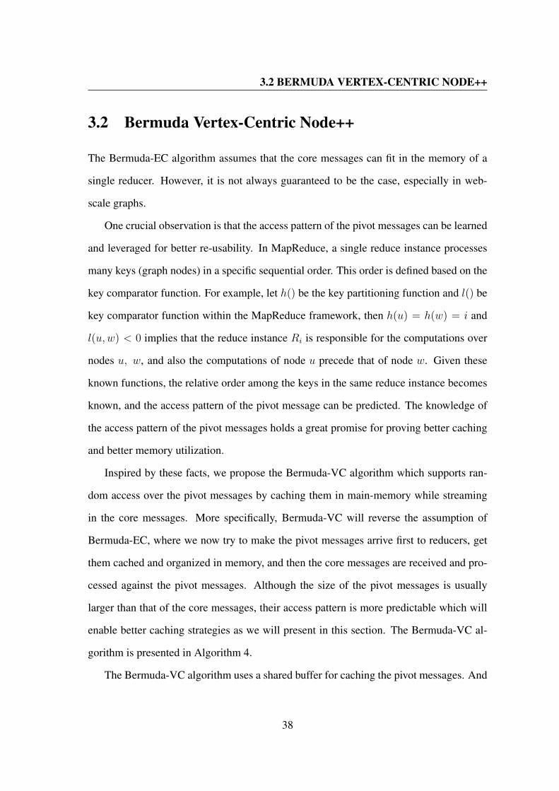
3.2 BERMUDA VERTEX-CENTRIC NODE++
3.2 Bermuda Vertex-Centric Node++
The Bermuda-EC algorithm assumes that the core messages can fit in the memory of a
single reducer. However, it is not always guaranteed to be the case, especially in web-
scale graphs.
One crucial observation is that the access pattern of the pivot messages can be learned
and leveraged for better re-usability. In MapReduce, a single reduce instance processes
many keys (graph nodes) in a specific sequential order. This order is defined based on the
key comparator function. For example, let h() be the key partitioning function and l() be
key comparator function within the MapReduce framework, then h(u) = h(w) = i and
l(u,w) < 0 implies that the reduce instance Ri is responsible for the computations over
nodes u, w, and also the computations of node u precede that of node w. Given these
known functions, the relative order among the keys in the same reduce instance becomes
known, and the access pattern of the pivot message can be predicted. The knowledge of
the access pattern of the pivot messages holds a great promise for proving better caching
and better memory utilization.
Inspired by these facts, we propose the Bermuda-VC algorithm which supports ran-
dom access over the pivot messages by caching them in main-memory while streaming
in the core messages. More specifically, Bermuda-VC will reverse the assumption of
Bermuda-EC, where we now try to make the pivot messages arrive first to reducers, get
them cached and organized in memory, and then the core messages are received and pro-
cessed against the pivot messages. Although the size of the pivot messages is usually
larger than that of the core messages, their access pattern is more predictable which will
enable better caching strategies as we will present in this section. The Bermuda-VC al-
gorithm is presented in Algorithm 4.
The Bermuda-VC algorithm uses a shared buffer for caching the pivot messages. And
38
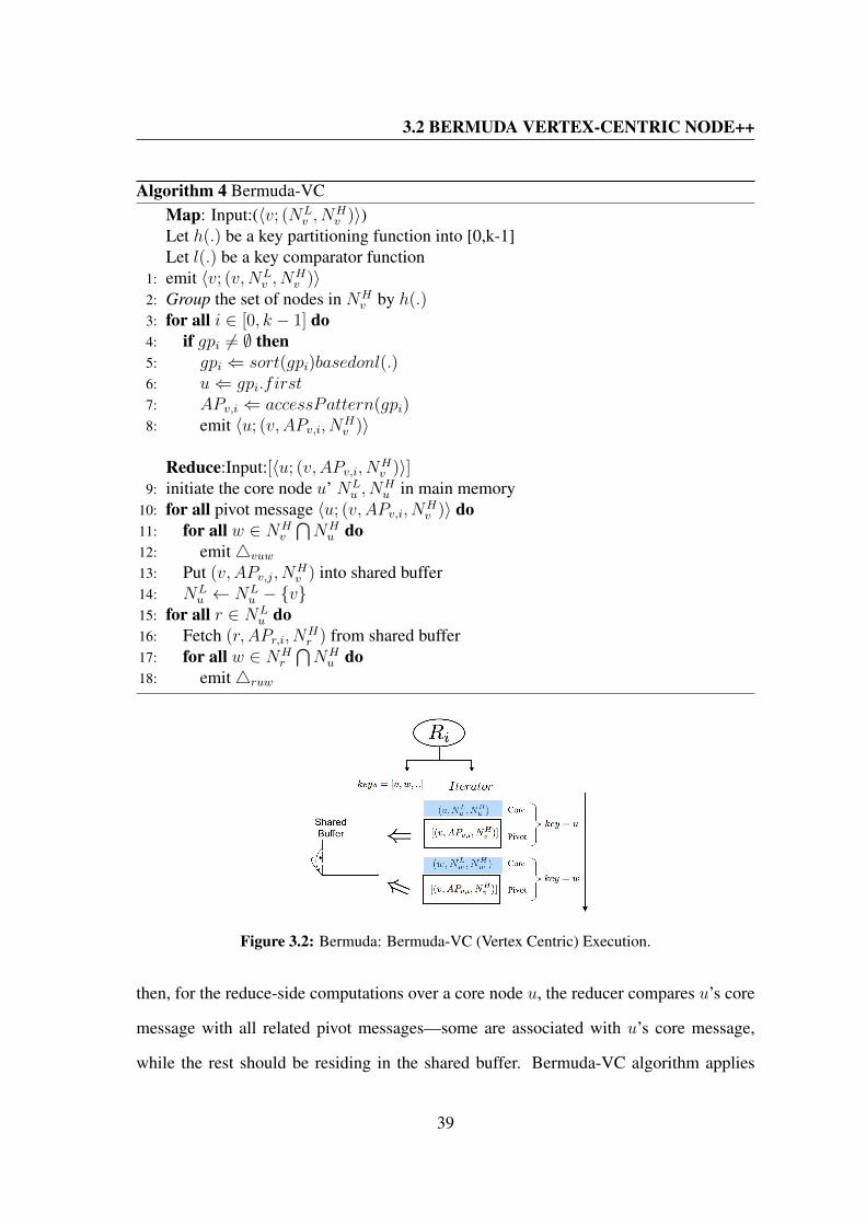
3.2 BERMUDA VERTEX-CENTRIC NODE++
Algorithm 4 Bermuda-VCMap: Input:(〈v; (NL
v , NHv )〉)
Let h(.) be a key partitioning function into [0,k-1]Let l(.) be a key comparator function
1: emit 〈v; (v,NLv , N
Hv )〉
2: Group the set of nodes in NHv by h(.)
3: for all i ∈ [0, k − 1] do4: if gpi 6= ∅ then5: gpi ⇐ sort(gpi)basedonl(.)6: u⇐ gpi.f irst7: APv,i ⇐ accessPattern(gpi)8: emit 〈u; (v,APv,i, N
Hv )〉
Reduce:Input:[〈u; (v,APv,i, NHv )〉]
9: initiate the core node u’ NLu , N
Hu in main memory
10: for all pivot message 〈u; (v,APv,i, NHv )〉 do
11: for all w ∈ NHv
⋂NHu do
12: emit4vuw
13: Put (v, APv,j, NHv ) into shared buffer
14: NLu ← NL
u − v15: for all r ∈ NL
u do16: Fetch (r, APr,i, N
Hr ) from shared buffer
17: for all w ∈ NHr
⋂NHu do
18: emit4ruw
Figure 3.2: Bermuda: Bermuda-VC (Vertex Centric) Execution.
then, for the reduce-side computations over a core node u, the reducer compares u’s core
message with all related pivot messages—some are associated with u’s core message,
while the rest should be residing in the shared buffer. Bermuda-VC algorithm applies
39

3.2 BERMUDA VERTEX-CENTRIC NODE++
the same scheme to avoid generating redundant pivot messages. It utilizes a universal
key partitioning function to group effective neighbors NHv of each node v. In order to
guarantee the availability of the pivot messages, a universal key comparator function is
utilized to sort the destination nodes in each group (Line 5, Algorithm 4). As a result,
destination nodes are sorted based on their processing order. The first node in group
gpi indicates the earliest request of a pivot message. Hence, each node v sends a pivot
message to the first node of each non-empty group by emitting key value pairs where key
equals the first node ID (Lines 6-8, Algorithm 4).
Combined with the sorting phase of the MapReduce framework, Bermuda-VC guar-
antees the availability of all needed pivot messages of any node u when u’s core message
is received by a reducer, i.e., the needed pivot messages are either associated with u itself
or associated with another nodes processed before u.
The reducers’ processing mechanism is similar to that of the MR-Baseline algorithm.
Each node u reads its core message for initiating NHu and NL
v (Line 9), and then it iterates
over every pivot message associated with key u against its effective adjacency list NHv to
enumerate the triangles (Lines 10-12). As discussed before, not all expected pivot mes-
sages are carried with key u. The rest of the related pivot messages reside in the shared
buffer. Here, NLv is used for fetching the rest of these pivot messages (Line 14, Algorithm
4), and enumerating the triangles (Lines 15-18, Algorithm 4). Moreover, the new com-
ing pivot messages associated with node u are pushed into the shared buffer for further
access by other nodes (Line 13). Figure 3.2 illustrates the reduce-side processing flow of
Bermuda-VC. In the following sections, we will discuss in more details the management
of the pivot messages in the shared buffer.
40
3.2 BERMUDA VERTEX-CENTRIC NODE++
3.2.1 Message Sharing Management
It is obvious that the best scenario is to have the shared buffer fits into the main memory of
each reduce instance. However, that cannot be guaranteed. In general, there are two types
of operations over the shared buffer inside a reduce instance, which are: “Put” for adding
new incoming pivot messages into the shared buffer (Line 13), and “Get” for retrieving
the needed pivot messages (Lines 15-18). For massive graphs, the main memory may
not hold all the pivot messages. This problem is similar to the classical caching problem
studied in [64, 65], where a reuse-distance factor is used to estimate the distances between
consecutive references of a given cached element, and based on that effective replacement
policies can be deployed. We adopt the same idea in Bermuda-VC.
Interestingly, in addition to the reuse distance, all access patterns of each pivot mes-
sage can be easily estimated in our context. The access pattern AP of a pivot message
is defined as the sequence of graph nodes (keys) that will reference this message. In
particular, the access pattern of a pivot message from node v to reduce instance Ri can
be computed based on the sorted effective nodes gpi received by Ri. Several interesting
metrics can be derived from this access pattern. For example, the first node in gpi indi-
cates the occurrence of the first reference, the size of gpi equals the cumulative reference
frequency. Such access pattern information is encoded within each pivot message (Lines
7-8, Algorithm 4). With the availability of this access pattern, effective message sharing
strategies can be deployed under limited memory.
As an illustrative example, Figure 3.3 depicts different access patterns for four pivot
messages m1, m2, m3, m4. The black bars indicate requests to the corresponding
pivot message, while the gaps represent the re-use distances (which are idle periods for
this message). Pivot messages may exhibit entirely different access patterns, e.g., pivot
message m1 is referenced only once, while others are utilized more than once, and some
pivot messages are used in dense consecutive pattern in a short interval, e.g., m2 and
41

3.2 BERMUDA VERTEX-CENTRIC NODE++
Figure 3.3: Bermuda: Access Patterns of Pivot Messages.
m3. Inspired by these observations, we propose two heuristic-based replacement policies,
namely usage-based tracking, and bucket-based tracking. They trade off the tracking
overhead with memory hits as will be described next.
3.2.1.1 Usage-Based Tracking
Given a pivot message originated from node v, the total use frequency is limited to√m,
referring to the number of its effective neighbors, which is much smaller than the expected
number of nodes processed in a single reducer, which is estimated to n/k. This implies
that each pivot message may become useless (and can be discard) as a reducer progresses,
and it is always desirable to detect the earliest time at which a pivot message can be
discarded to maximize the memory’s utilization.
The main idea of the usage-based tracking is to use a usage counter per pivot message
in the shared buffer. And then, the tracking is performed as follows. Each Put operation
sets the counter as the total use frequency. And, only the pivot messages whose usage
counter is larger than zero are added to the shared buffer. Each Get operation decre-
ments the counter of the target pivot message by one. Once the counter reached zero, the
corresponding pivot message is evicted from the shared buffer.
The usage-based scheme may fall short in optimizing sparse and scattered access pat-
terns. For example, as shown in Figure 3.3, the reuse distance of message m4 is large.
42

3.2 BERMUDA VERTEX-CENTRIC NODE++
Figure 3.4: Bermuda: The Usage of External Memory.
Therefore, the usage-based tracking strategy has to keep m4 in the shared buffer although
it will not be referenced for a long time. What’s worse, such scattered access is common
in massive graphs. Therefore, pivot messages may unnecessarily overwhelm the available
memory of each single reduce instance.
3.2.1.2 Bucket-Based Tracking
We introduce the Bucket-based tracking strategy to optimize message sharing over scat-
tered access patterns. The main idea is to manage the access patterns of each pivot mes-
sage at a smaller granularity, called a bucket. The processing sequence of keys/nodesis
sliced into buckets as illustrated in Figure 3.3. In this work, we use the range partitioning
method for balancing workload among buckets. Correspondingly, the usage counter of
one pivot message is defined per bucket, i.e., each message will have an array of usage
counters of a length equals to the number of its buckets. For example, the usage count of
m4 in the first bucket is 1 while in the second bucket is 0. Therefore, for a pivot message
that will remain idle (with no reference) for a long time, its counter array will have a long
sequence of adjacent zeros. Such access pattern information can be computed in the map
function, encoded in access pattern (Line 7 in Algorithm 4), and passed to the reduce side.
The corresponding modification of the Put operation is as follows. Each new pivot
message will be pushed into the shared buffer (in memory) and backed up by local files
43
3.2 BERMUDA VERTEX-CENTRIC NODE++
(in disk) based on its access pattern. Figure 3.4 illustrates this procedure. For the arrival
of a pivot message with the access pattern [1, 0, .., 1, 3], the reduce instance actively adds
this message into back-up files for bucketsBp−1 (next-to-last bucket) andBp (last bucket).
And then, at the end of each bucket processing and before the start of processing the next
bucket, all pivot messages in the shared buffer are discarded, and a new set of pivot
messages is fetched from the corresponding back-up file into memory(See Figure 3.4).
The Bucket-based tracking strategy provides better memory utilization since it pre-
vents the long retention of unnecessary pivot messages. In addition, usage-based tracking
can be applied to each bucket to combine both benefits, which is referred to as the bucket-
usage tracking strategy.
3.2.2 Analysis of Bermuda-VC
In this section, we show the benefits of the Bermuda-VC algorithm over the Bermuda-EC
algorithm. Furthermore, we discuss the effect of parameter p, which is the the number of
buckets, on the performance.
Under the same settings of the number of reducers k, the Bermuda-VC algorithm gen-
erates more intermediate message and takes longer execution time. Firstly, the Bermuda-
VC algorithm generates the same number of pivot messages while generating more core
messages (i.e., additional NLv for reference in the reduce side). Thus, the total size of the
extra NLv core message is
∑v∈V N
Lv = m. Such noticeable size of extra core messages
requires additional time for generating and shuffling. Moreover, an additional computa-
tional overhead (Lines 13-14) is required for the message sharing management.
However, because of the proposed sharing strategies, the Bermuda-VC algorithm can
work under smaller settings for k—which are settings under which the Bermuda-EC al-
gorithm will probably fail. In this case, the benefits brought by having a smaller k will
exceed the corresponding cost. In such cases, Bermuda-VC algorithm will outperform
44

3.2 BERMUDA VERTEX-CENTRIC NODE++
Bermuda-EC algorithm.
Moreover, compared to the disk-based Bermuda-EC algorithm, the Bermuda-VC al-
gorithm has a relatively smaller disk I/O cost because the predictability of the access
pattern of the pivot messages, which enable purging them early, while that is not applica-
ble to the core messages. Notice that, for any given reduce instance, the expected usage
count of pivot message from u is dHu /k. Thus, the expected usage count for any pivot
message is E(dHu )/k, equals m/nk. Therefore, the total disk I/O with pivot messages is
at most m2/nk, smaller than disk I/O cost of Bermuda-EC algorithm m2/Mk, where M
stands for the size of the available memory in a single machine.
Effect of the number of buckets p: At a high level, p trades off the space used by
the shared buffer with the I/O cost for writing and reading the back-up files. Bermuda-VC
algorithm favors smaller settings of p in the capacity of main-memory. As p decreases,
the expected number of reading and writing decreases, however the total size of the pivot
messages in the shared buffer may exceed the capacity of the main-memory. For a setting
of p, the expected size of the pivot messages for any bucket is O(m/kp). Therefore, a
visible solution for O(m/kp) ≤ M is ≥ O(m/kM). In this work, p is set as O(m/kM)
where m is the size of the input graph, and M is the size of the available memory in a
single machine.
45

4
Performance Evaluation
In this section, we present an experimental evaluation of the MR-Baseline, Bermuda-
EC, and Bermuda-VC algorithms. We also compare Bermuda algorithms against GP
(Graph Partitioning algorithm for triangle listing) [13]. The objective of our experimental
evaluation is to show that the proposed Bermuda method improves both time and space
complexity compared to the MR-Baseline algorithm. Moreover, compared to Bermuda-
EC, Bermuda-VC is able to get better performance under the proposed message caching
strategies.
All experiments are performed on a shared-nothing computer cluster of 30 nodes.
Each node consists of one quad-core Intel Core Duo 2.6GHZ processors, 8GB RAM,
400GB disk, and interconnected by 1Gb Internet. Each node runs Linux OS and Hadoop
version 2.4.1. Each node is configured to run up to 4 map and 2 reduce tasks concurrently.
The replication factor is set to 3 unless otherwise is stated.
46

4.1 DATASETS
NodesUndirected
EdgesAvg
Degree Size
Twitter 4.2 ∗ 107 2.4 ∗ 109 57 24GBYahoo 1.9 ∗ 108 9.0 ∗ 109 47 67GBClueWeb12 9.6 ∗ 108 8.2 ∗ 1010 85 688GB
Table 4.1: Bermuda: Basic Statistics about Datasets.
4.1 Datasets
We use three large real-world graph datasets for our evaluation. Twitter is one represen-
tative social network which captures current biggest micro-blogging community. Edges
represent the friendship among users 1. Yahoo is one of the largest real-world web graphs
with over one billion vertices 2, where edges represent the link among web pages. And
ClueWeb12 is one subset of real-world web with six billion vertices 3.
In our experiments, we consider each edge of the input to be undirected. Thus, if
an edge (u,v) appears in the input, we also add edge (v, u) if it does not already exist.
The graph sizes varies from 4.2 ∗ 107 of Twitter , 1.9 ∗ 108 of Yahoo, to 9.6 ∗ 108 of
ClueWeb12, with different densities; ClueWeb12 is the largest but also the sparest dataset.
The statistics on the three datasets are presented in Table 4.1.
4.2 Experiment Result
MRBaseline
BermudaEC and VC
ReductionFactor (RF)
Twitter 3.0 ∗ 1011 1.2 ∗ 1010 30Yahoo 1.4 ∗ 1011 1.9 ∗ 1010 7.5ClueWeb12 3.0 ∗ 1012# 2.6 ∗ 1011 11.5
Table 4.2: Bermuda: Reduction Factors of Communication Cost.
1http://an.kaist.ac.kr/traces/WWW2010.html2http://webscope.sandbox.yahoo.com.20153http://www.lemurproject.org /clueweb12/webgraph.php/.
47
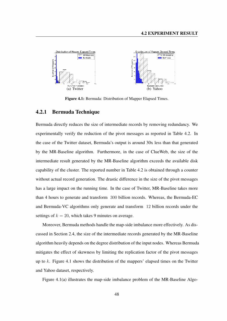
4.2 EXPERIMENT RESULT
(a) Twitter (b) Yahoo
Figure 4.1: Bermuda: Distribution of Mapper Elapsed Times.
4.2.1 Bermuda Technique
Bermuda directly reduces the size of intermediate records by removing redundancy. We
experimentally verify the reduction of the pivot messages as reported in Table 4.2. In
the case of the Twitter dataset, Bermuda’s output is around 30x less than that generated
by the MR-Baseline algorithm. Furthermore, in the case of ClueWeb, the size of the
intermediate result generated by the MR-Baseline algorithm exceeds the available disk
capability of the cluster. The reported number in Table 4.2 is obtained through a counter
without actual record generation. The drastic difference in the size of the pivot messages
has a large impact on the running time. In the case of Twitter, MR-Baseline takes more
than 4 hours to generate and transform 300 billion records. Whereas, the Bermuda-EC
and Bermuda-VC algorithms only generate and transform 12 billion records under the
settings of k = 20, which takes 9 minutes on average.
Moreover, Bermuda methods handle the map-side imbalance more effectively. As dis-
cussed in Section 2.4, the size of the intermediate records generated by the MR-Baseline
algorithm heavily depends on the degree distribution of the input nodes. Whereas Bermuda
mitigates the effect of skewness by limiting the replication factor of the pivot messages
up to k. Figure 4.1 shows the distribution of the mappers’ elapsed times on the Twitter
and Yahoo dataset, respectively.
Figure 4.1(a) illustrates the map-side imbalance problem of the MR-Baseline Algo-
48

4.2 EXPERIMENT RESULT
Figure 4.2: Bermuda: Disk Space vs.Memory Tradeoff.
Figure 4.3: Bermuda: Running Time ofBermuda-EC.
rithm as indicated by the heavy-tailed distribution of the elapsed time (the x-axis). The
majority of the map tasks finish in less than 100 minutes, but there are a handful of map
tasks that take more than 200 minutes. The mappers that have the longest completion
time received high degree nodes to pivot on. This is because for a node of effective de-
gree d, the MR-Baseline algorithm generates O(d2) pivot messages. Figure 4.1(a) shows
a significantly more balanced workload distribution under the Bermuda algorithms. This
is indicated by a smaller spread out between the fastest and slowest mappers , which is
around 10 minutes. This is because for a node of effective degree d, Bermuda would gen-
erate only O(min(k, d)d) pivot messages. Therefore, the variance of mappers’ outputs is
significantly reduced. Figure 4.1(b) manifests the same behavior over the Yahoo dataset.
This empirical observation is in accordance with our theoretical analysis and Theorems 2
and 4. Thus, Bermuda methods outperform the MR-Baseline Algorithm.
4.2.2 Effect of the number of reducers
In Bermuda-EC, the number of reducers k trades off between the memory used by each
reducer and the used disk space. Figure 4.2 illustrates such trade off on the Twitter and
Yahoo datasets. Initially, as k increases, the increase of the storage overhead is small
while the reduction of memory is drastic. In the case of the Yahoo dataset, as k increases,
the size of the core messages decreases, and can fit in the available main-memory. As
49
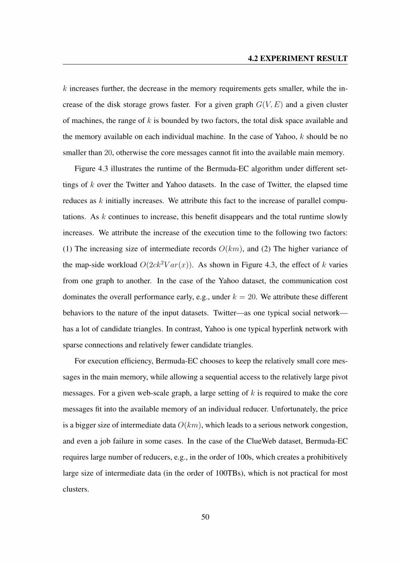
4.2 EXPERIMENT RESULT
k increases further, the decrease in the memory requirements gets smaller, while the in-
crease of the disk storage grows faster. For a given graph G(V,E) and a given cluster
of machines, the range of k is bounded by two factors, the total disk space available and
the memory available on each individual machine. In the case of Yahoo, k should be no
smaller than 20, otherwise the core messages cannot fit into the available main memory.
Figure 4.3 illustrates the runtime of the Bermuda-EC algorithm under different set-
tings of k over the Twitter and Yahoo datasets. In the case of Twitter, the elapsed time
reduces as k initially increases. We attribute this fact to the increase of parallel compu-
tations. As k continues to increase, this benefit disappears and the total runtime slowly
increases. We attribute the increase of the execution time to the following two factors:
(1) The increasing size of intermediate records O(km), and (2) The higher variance of
the map-side workload O(2ck2V ar(x)). As shown in Figure 4.3, the effect of k varies
from one graph to another. In the case of the Yahoo dataset, the communication cost
dominates the overall performance early, e.g., under k = 20. We attribute these different
behaviors to the nature of the input datasets. Twitter—as one typical social network—
has a lot of candidate triangles. In contrast, Yahoo is one typical hyperlink network with
sparse connections and relatively fewer candidate triangles.
For execution efficiency, Bermuda-EC chooses to keep the relatively small core mes-
sages in the main memory, while allowing a sequential access to the relatively large pivot
messages. For a given web-scale graph, a large setting of k is required to make the core
messages fit into the available memory of an individual reducer. Unfortunately, the price
is a bigger size of intermediate data O(km), which leads to a serious network congestion,
and even a job failure in some cases. In the case of the ClueWeb dataset, Bermuda-EC
requires large number of reducers, e.g., in the order of 100s, which creates a prohibitively
large size of intermediate data (in the order of 100TBs), which is not practical for most
clusters.
50

4.2 EXPERIMENT RESULT
Figure 4.4: Bermuda (disk-based): Vary-ing k vs. Running Time.
Reduce Progress0 0.1 0.2 0.3 0.4 0.5 0.6 0.7 0.8 0.9 1
Me
mo
ry U
sa
ge
(G
B)
0
1
2
3
4
5
6
7
8
9
Max-MemoryNo TrackingUsageBucketBucket-Usage
Figure 4.5: Bermuda: The Accumula-tion of Sharing Messages.
Although the disk-based Bermuda-EC algorithm can work under smaller settings of
k, its efficiency is limited because of a large amount of disk I/Os. Figure 4.4 presents the
run time of the disk-based Bermuda-EC variation under different settings of k over the
Yahoo dataset. When k ≥ 20, the core messages can fit into memory, and its runtime is
presented in Figure 4.3. When k equals 10, the disk-based Bermuda-EC algorithm takes
less time in generating and shuffling the intermediate data, while more time is taken in
the reduce phase. As expected, the runtime of the reduce step increases quickly and the
benefits induced by the smaller settings of k disappear.
4.2.3 Message Sharing Management
In Figure 4.5, we present the empirical results of the different caching strategies on the
Yahoo dataset where k = 10. As shown in Figure 4.5, the size of sharing messages grows
rapidly, then overwhelms the size of the main memory available to a given reducer, which
leads to a job failure. By tracking the re-use count, the usage-based tracking strategy is
able to immediately discard useless pivot messages when their counter reaches zero. As
a result the increase of the memory usage is slower. However, the retention of the pivot
message having long re-use distance makes the discard strategy not very effective. By
51

4.2 EXPERIMENT RESULT
MR-Baseline GP
Bermuda-EC
Bermuda-VC
Twitter 682 378 52 66Yahoo 439 622 82 69
ClueWeb12 − − − 1528
Table 4.3: Bermuda: Effectiveness Evaluation.
considering the access pattern of the pivot messages at a smaller granularity, the bucket-
based strategy avoids the retention of the pivot messages having too long re-use distance.
As shown in Figure 4.5, the bucket-based strategy achieves better memory utilization. In
the case of the Yahoo dataset, the size of sharing pivot message is practical for a com-
modity machine with the bucket-based strategy. The combination of the two strategies,
i.e., the bucket-usage strategy can further reduce the size of sharing message by avoiding
the memory storage of idle messages inside each bucket.
4.2.4 Execution Time Performance
Table 4.3 presents the runtime of all algorithms on the three datasets. For the Bermuda-
EC algorithm, the number of reducers k is set to 40 and 20, for the Twitter and Yahoo
datasets, respectively. For the Bermuda-VC algorithm, the number of reducers k is set
to 40, 10, and 10, for the Twitter, Yahoo and ClueWeb datasets, respectively. The set-
tings of reducer number k are determined by the cluster and the given datasets. Only
Bermuda-VC manages to list all triangles in ClueWeb dataset, whereas MR-Baseline, GP
and Bermuda-EC fail to finish due to the lack of disk space. As shown in Table 4.3,
Bermuda methods outperform the other algorithms on the Twitter and Yahoo datasets.
Bermuda-EC algorithm shows more than 5x faster performance on the Twitter dataset
compared to the GP algorithm. Moreover, compared to Bermuda-EC, Bermuda-VC is
able to get a better trade-off between the communication cost and the reduce-side compu-
tations. It shows a better performance over the Yahoo dataset under k = 10. Moreover,
52

4.2 EXPERIMENT RESULT
with a relatively small cluster, Bermuda-VC can scale up to larger datasets, e.g., ClueWeb
graph dataset (688GB), while the other techniques fail to finish.
53

5
Related Works
Triangle listing is a basic operation of the graph analysis. Many research works have been
conducted on this problem, which can be classified into three categories: in-memory algo-
rithms, external-memory algorithms and distributed algorithms. Here, we briefly review
these works.
In-Memory Algorithm. The majority of previously introduced triangle listing al-
gorithms are the In-Memory processing approaches. Traditionally, they can be further
classified as Node-Iterator[35, 36, 37] and Edge-Iterator ones[38, 39] with the respect to
iterator-type. Authors [37, 38, 39]improved the performance of in-memory algorithms
by adopting degree-based ordering. Matrix multiplication is used to count triangles [35].
However, all these algorithms are inapplicable to massive graphs which do not fit in mem-
ory.
External-Memory Algorithms. In order to handle the massive graph, several external-
memory approaches were introduced [9, 10, 11]. Common idea of these methods is:
(1) Partition the input graph to make each partition fit into main-memory, (2) Load each
partition individually into main-memory and identify all its triangles, and then remove
edges which participated in the identified triangle, and (3) After the whole graph is loaded
54

into memory buffer once, the remaining edges are merged, then repeat former steps until
no edges remain. These Algorithms require a lot of disk I/Os to perform the reading and
writing of the edges. Authors [9, 10] improved the performance by reducing the amount
of disk I/Os and exploiting multi-core parallelism. External-Memory Algorithms show
great performance in time and space. However, the parallelization of external-memory
algorithms is limited. External-memory approaches cannot easily scale up in terms of
computing resources and parallelization degree.
Distributed Algorithms. Another promising approach to handle triangle listing on
large-scale graphs is the distributed computing. Suri et al. [13] introduced two Map-
Reduce adaption of NodeIterator algorithm and the well-known Graph Partitioning (GP)
algorithm to count triangles. The Graph Partitioning algorithm utilizes one universal hash
partition function over nodes to distribute edges into overlapped graph partitions, then
identifies triangles over all the partitions. Park et al. [40] further generalized Graph Par-
titioning algorithm into multiple rounds, significantly increasing the size of the graphs
that can be handled on a given system. The authors compare their algorithm with GP
algorithm [13] across various massive graphs then show that they get speedups ranging
from 2 to 5. In this work, we show such large or even larger speedup (from 5 to 10)
can also be obtained by reducing the size intermediate result directly via Bermuda meth-
ods. Teixeira et al. [41] presented Arabesque, one distributed data processing platform
for implementing subgraph mining algorithms on the basis of MapReduce framework.
Arabesque automates the process of exploring a very large number of subgraphs, includ-
ing triangles. However, these MapReduce algorithms must generate a large amount of
intermediate data that travel over the network during the shuffle operation, which degrade
their performance. Arifuzzaman et al. [12] introduced an efficient MPI-based distributed
memory parallel algorithm (Patric) on the basis of NodeIterator algorithm. The Patric al-
gorithm introduced degree-based sorting preprocessing step for efficient set intersection
55

operation to speed up execution. Furthermore, several distributed solutions designed for
subgraph mining on large graph were also proposed [1, 42]. Shao et al. introduced the
PSgl framework to iteratively enumerate subgraph instance. Different from other parallel
approaches, the PSgl framework completes relies on the graph traversal and avoids the
explicit join operation. These distributed memory parallel algorithms achieve impressive
performance over large-scale graph mining tasks. These methods distributed the data
graph among the worker’s memory, thus they are not suitable for processing large-scale
graph with small clusters.
56

Part II
Resisting Degree-based
De-anonymization in Anonymized
Uncertain Graphs
57

6
Problem Definition
In this section, we present the models of uncertain graph, privacy criteria, and utility met-
ric. We then present the formal formulation of uncertain graph anonymization problem.
6.1 Uncertain Graph
Let G = (V,E, p) be an uncertain graph, where V is the set of nodes,E is the set of edges,
and function p : E → [0, 1] assigns a probability of existence to each edge, denoted as
p(e). In this paper, we assume the possible world semantics where the edge probabilities
are independent of each other, which is a common assumption in uncertain graph ana-
lytics [17, 18, 23, 66, 67, 68]. Specifically, the possible world semantics interprets G as
a set of possible deterministic graphs W (G) = G1, G2, ..., Gn, where each determin-
istic graph Gi ∈ W (G) includes all vertices of G and a subset of edges EGi ⊂ E. The
probability of observing any possible world Gi = (V,EGi) ∈ W (G) is
Pr[Gi] =∏e∈EGi
p(e)∏
e∈E\EGi
(1− p(e))
In this work, we assume the input uncertain graph undirected and contains no self-
58
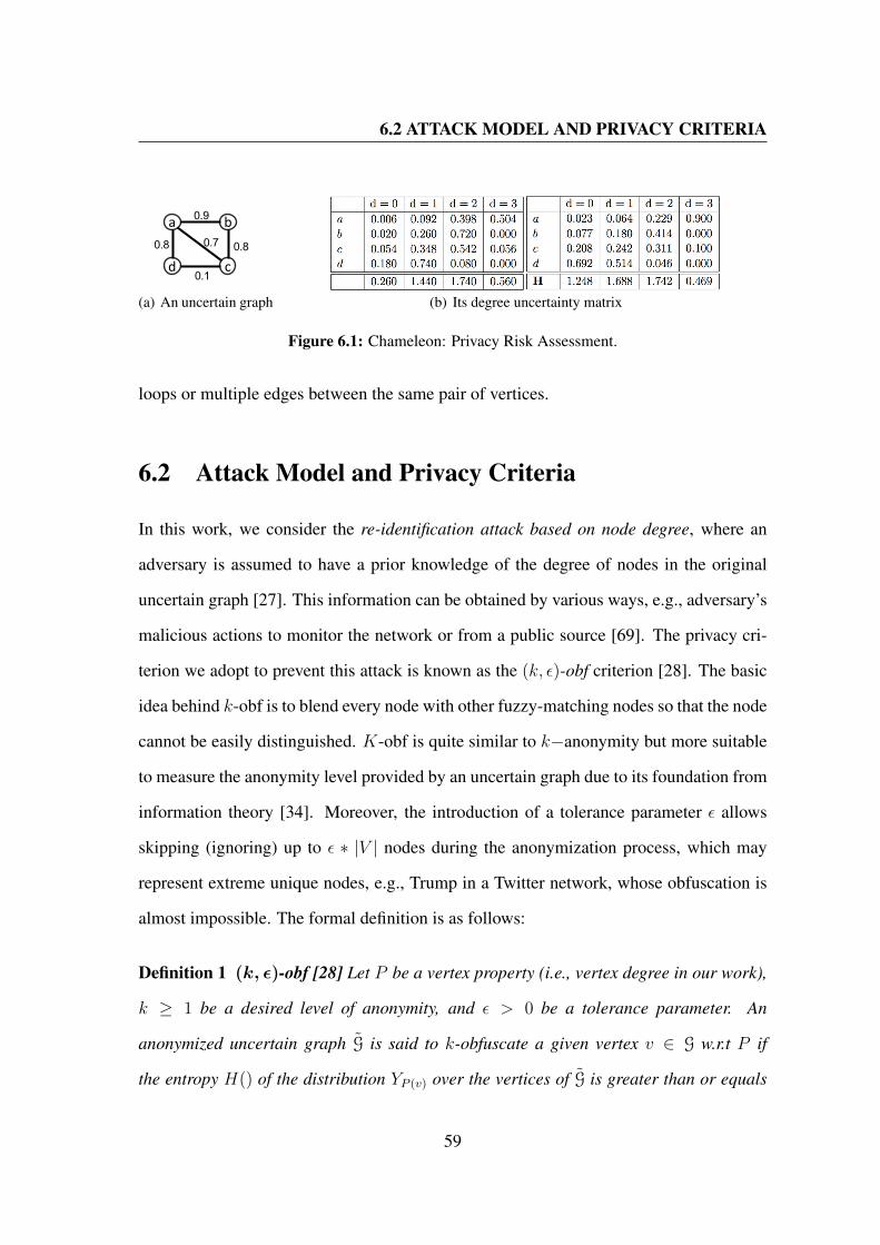
6.2 ATTACK MODEL AND PRIVACY CRITERIA
0.9
0.8
0.1
0.80.7
a
d c
b
(a) An uncertain graph (b) Its degree uncertainty matrix
Figure 6.1: Chameleon: Privacy Risk Assessment.
loops or multiple edges between the same pair of vertices.
6.2 Attack Model and Privacy Criteria
In this work, we consider the re-identification attack based on node degree, where an
adversary is assumed to have a prior knowledge of the degree of nodes in the original
uncertain graph [27]. This information can be obtained by various ways, e.g., adversary’s
malicious actions to monitor the network or from a public source [69]. The privacy cri-
terion we adopt to prevent this attack is known as the (k, ε)-obf criterion [28]. The basic
idea behind k-obf is to blend every node with other fuzzy-matching nodes so that the node
cannot be easily distinguished. K-obf is quite similar to k−anonymity but more suitable
to measure the anonymity level provided by an uncertain graph due to its foundation from
information theory [34]. Moreover, the introduction of a tolerance parameter ε allows
skipping (ignoring) up to ε ∗ |V | nodes during the anonymization process, which may
represent extreme unique nodes, e.g., Trump in a Twitter network, whose obfuscation is
almost impossible. The formal definition is as follows:
Definition 1 (k, ε)-obf [28] Let P be a vertex property (i.e., vertex degree in our work),
k ≥ 1 be a desired level of anonymity, and ε > 0 be a tolerance parameter. An
anonymized uncertain graph G is said to k-obfuscate a given vertex v ∈ G w.r.t P if
the entropy H() of the distribution YP (v) over the vertices of G is greater than or equals
59

6.3 RELIABILITY-BASED UTILITY LOSS METRIC
to log2 k:
H(YP (v)) ≥ log2 k.
The uncertain graph G is (k, ε)-obf w.r.t property P if it k-obfuscates at least (1 − ε)|V |
vertices in G.
Figure 6.1(b) gives an example of how to compute the degree entropy for the uncertain
graph in Figure 6.1(a). Here, the vertex property P represent the node degree. Each
row in the L.H.S table represents the degree distribution of the corresponding node. For
example, Node a has degree 0 with probability 0.006. The R.H.S table normalizes the
values in each column (i.e. over each degree value d) to get a distributions YP (v). The
entropy H(YP (v)) is then computed for each degree (one column in the R.H.S table) as
shown in bottom row.
6.3 Reliability-Based Utility Loss Metric
Reliability generalizes the concept of connectivity by capturing the probability that two
given (sets of) nodes are reachable over all possible worlds of the uncertain graph. And,
reliability forms the foundation of numerous uncertain graph theoretic algorithms such as
k−nearest neighbors[18, 66], shortest paths detecting [23, 58]. It is the core interest of
uncertain graph analysis tasks, therefore it should be well-preserved in the anonymization
process.
Inspired by its significance, we propose a novel utility loss metric that is based on reli-
ability (connectivity-based graph model). Specifically, we use the two-terminal reliability
difference to reflect the impact of anonymization on uncertain graph structure(referred to
as Reliability Discrepancy).
Definition 2 Two-Terminal Reliability [70] Given an uncertain graph G, and two distinct
60

6.4 PROBLEM STATEMENT
nodes u and v ∈ V , the reliability of (u, v) is defined as:
Ru,v(G) =∑
G∈W (G)
IG(u, v)Pr[G]
where Pr[G] is the probability of observingG as one possible world of G, and IG(u, v)
is 1 iff u and v are contained in a connected component in G, and 0 otherwise.
Definition 3 Graph Reliability Discrepancy The reliability discrepancy of graph G =
(V,E, p), denoted as ∆(G), w.r.t. an original graph G = (V,E, p) is defined as the sum
of the two-terminal reliability discrepancy over all node pair (u, v) ∈ VG.
∆(G) =∑
(u,v)∈VG
|Ru,v(G)−Ru,v(G)|
6.4 Problem Statement
Given the above foundation, we can now formulate the addressed problem.
Problem 1 Reliability-Preserving Uncertain Graph Anonymization Given an uncertain
graph G = (V,E, p) and anonymization parameters k and ε, the objective is to find a
(k, ε)-obfuscated uncertain graph G = (V,E, p) with minimal ∆(G). That is:
argminG
∆(G)
Subject to G is (k, ε)− obf
61
7
Uncertain Graph Anonymization via
Representative Instance
One baseline approach for anonymizing an uncertain graph G involves two phases that
combine isolated but complementary work from literature. First is to somehow transform
G to one deterministic representative graph (Say G), and then use any technique from the
“uncertainty semantic-based modification” category [28, 29, 30] to generate anonymous
uncertain graphs (See top part of Figure 7.1). Fortunately, few techniques have been re-
cently proposed for exacting representative deterministic graphs from an uncertain graph
while capturing the key properties of the uncertain graph [71].
The advantage of this approach, which we refer to as Rep-An (a short name for Rep-
resentative Anonymization), is that it does not require new anonymization techniques.
However, the disadvantages of Rep-An are multifold. First, the input edge uncertain-
ties (probabilities) are no longer integrated into the anonymization process since they are
detached from the graph in the first phase. Second, the anonymization process (the sec-
ond phase) is oblivious to the reliability metric since its input is a made-up deterministic
graph. Third, since the two phases are isolated from each other, each phase optimizes for
62
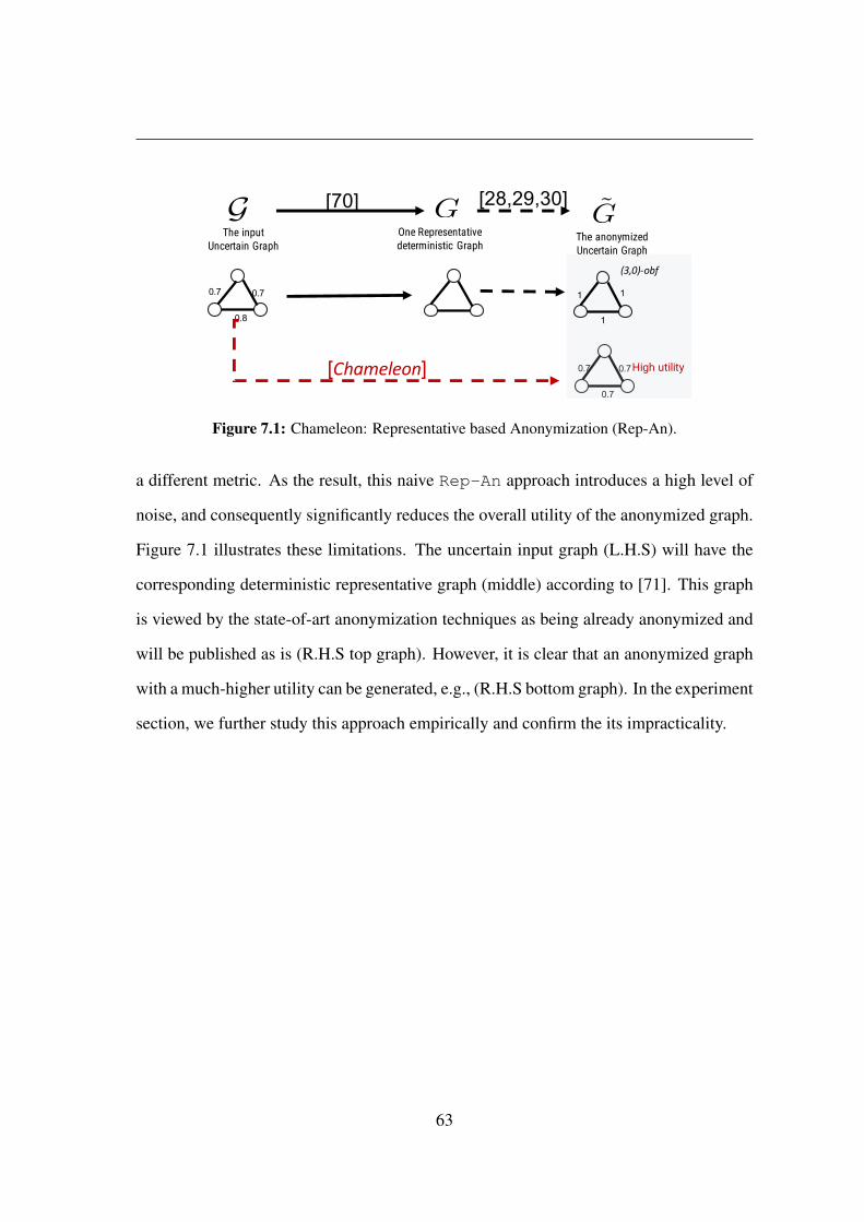
The anonymizedUncertain Graph
One Representativedeterministic Graph
The inputUncertain Graph
G G G
0.7
0.8
0.7
0.7
0.7
0.7
[70] [28,29,30]
[Chameleon]
1
1
1
(3,0)-obf
High utility
Figure 7.1: Chameleon: Representative based Anonymization (Rep-An).
a different metric. As the result, this naive Rep-An approach introduces a high level of
noise, and consequently significantly reduces the overall utility of the anonymized graph.
Figure 7.1 illustrates these limitations. The uncertain input graph (L.H.S) will have the
corresponding deterministic representative graph (middle) according to [71]. This graph
is viewed by the state-of-art anonymization techniques as being already anonymized and
will be published as is (R.H.S top graph). However, it is clear that an anonymized graph
with a much-higher utility can be generated, e.g., (R.H.S bottom graph). In the experiment
section, we further study this approach empirically and confirm the its impracticality.
63

8
Chameleon Framework
We first describe the general iterative skeleton of Chameleon, and then present in detail
the two core steps in each iteration, namely edge selection and perturbation injection, in
Sections 8.2 and 8.4, respectively.
8.1 Chameleon Iterative Skeleton
Algorithm 5 presents the skeleton of the framework. It takes as inputs the original uncer-
tain graph G, the adversary knowledge K representing the nodes degrees in G, the privacy
parameters k and ε, and two other parameters, which will be described later. The output
is an anonymized graph Gobf that has the same set of vertices but a modified set of edges.
The core function of the process is the GenerateObfuscation function (Lines 3 &
8), which performs two key tasks; first selecting a subset of edges to alter, and second
deciding on the amount of noise to inject into these edges.
In general, G can have up to |V |(|V | − 1)/2 edges. In each execution of
GenerateObfuscation(), a relatively small candidate set of these edges Ec is se-
lected for perturbation, which is controlled by the input parameter c > 1 (multiplier fac-
64

8.1 CHAMELEON ITERATIVE SKELETON
tor), i.e., |Ec| = c|E|. And then, the function will inject some probability noise over each
edge e ∈ Ec. To simulate the stochastic process, the amount of injected noise re ∈ [0, 1]
follows the [0, 1]-truncated normal distribution:
Rσ(r) :=
Φ0,σ(r)∫ 1
0 Φ0,σ(x)dxr ∈ [0, 1]
0 otherwise(8.1)
where Φ0,σ is the density function of a Gaussian distribution with a standard variation
σ. As σ decreases, a greater mass of Rσ will be concentrated near r = 0, and thus the
amount of perturbation r will be smaller. In other words, the smaller the σ the less noise
is injected and the higher the utility of the published graph. More details on these two
steps will be presented in the following two sections.
Algorithm 5 Chameleon Iterative SkeletonInput: Uncertain graph G, adversary knowledge K, obfuscation level k, tolerancelevel ε, size multiplier c and white noise level qOutput: The anonymized result Gobf
1: σl ← 0; σu ← 12: repeat3: 〈ε, G〉 ← GenerateObfuscation(G, k, ε, c, q, σu,K)4: if ε = 1 (fail) then σl ← σu; σu ← 2σu5: until ε 6= 16: repeat7: σ ← (σu + σl)/28: 〈ε, G〉 ← GenerateObfuscation(G, k, ε, c, q, σu,K)9: if ε = 1 then σl ← σ
10: else σu ← σ; Gobf ← G
11: until σu − σl is enough small12: return Gobf
The iterative algorithm starts with an initial guess on the upper bound for σ, which is
σu = 1 (Line 1). And then, it enters a loop trying to find a successful initial (k, ε)-obf
for the graph (Lines 2-5). With each failed attempt, it doubles the σu to allow for more
noise to be injected (Lines 4). After a successful attempt, the algorithm enters its second
65

8.2 HYBRID EDGE SELECTION
loop, which is a binary search process over the found low bound σl and upper bound σu
(Lines 7-11). The binary search terminates when the search interval is sufficiently short,
and the algorithm outputs the best (k, ε)-obf graph, which is the last one obtained with
the smallest σ.
This general iterative skeleton is similar to the one proposed in [28]. However, they
fundamentally differ in the core function GenerateObfuscation (Line 3 & 8). The
method proposed in [28] has two limitations when considering uncertain graphs anonymiza-
tion. First, the method does not consider the structural relevance of edges in the critical
edge selection step, which leads to unnecessary structural distortion. Second, its scheme
assumes the existence of edges is known with certainty, thus fails to handle uncertain
graphs where the existence of edges is probabilistic.
8.2 Hybrid Edge Selection
As discussed in Chapter 8, the first step inside the GenerateObfuscation() func-
tion is to select a subset of candidate edges for obfuscation. Figuring out the optimal
subset of edges that balances the privacy gain and the utility loss is a typical combina-
tional optimization problem. It involves the consideration over the exponential number of
edge combinations. Let alone the infinite possibilities of probability values on the selected
edges, which further complicates the problem.
In the context of deterministic graphs, various heuristics have been utilized [32, 50,
72] to alleviate the combinational intractability. These heuristics can be classified into two
main categories: (1) Anonymity-oriented heuristics that suggest injecting larger perturba-
tions to the edges associated with the less-anonymized (more-unique) nodes [27, 28, 31,
32, 33, 43, 44, 50, 54, 72, 73, 74], and (2) Utility-oriented heuristics that suggest avoiding
perturbations over “bridge” and sensitive edges whose deletion or addition would signif-
66
8.2 HYBRID EDGE SELECTION
icantly impact the graph structure [31, 32, 33, 43, 54, 72, 74]. It is clear that these two
types are complementary to each other and combining them would introduce an added
benefit as confirmed by practice in deterministic graph anonymization [72]. Neverthe-
less, these two types of heuristics and their combination have not been explored yet in the
context of uncertain graphs.
Therefore, for the edge selection step in Chameleon, we (1) Introduce a novel edge
relevance metric, called reliability relevance (RR), for quantifying the impact of edge
modifications on the overall uncertain graph reliability, (2) Present an efficient algorithm
for reliability relevance evaluation (3) Propose a hybrid heuristic that combines unique-
ness with reliability relevance. On this basis, we propose a sampling-based approach to
identify the candidate subset of edge efficiently.
8.2.1 Uniqueness Score
Uniqueness score is proposed in [28] as a relative measure indicating how common (or
unique) a given node is among the other nodes in the graph w.r.t a specific property, e.g.,
node degree. The definition is given as follows.
Definition 4 Uniqueness Score [28] Let P : V → ΩP be a property on the set of
nodes V of graph G, let d be a distance function on ΩP , and θ > 0 a positive in-
teger parameter. Then, the θ-commonness of a property values ω ∈ ΩP is Cθ(ω) =∑u∈V Φ0,θ(d(ω, P (v))), while the θ-uniqueness of ω ∈ ΩP is Uθ = 1
Cθ(ω).
In a simplified explanation, the commonness of the property value ω is a measure
of how typical is the value ω among the vertices of the graph (density estimation). The
uniqueness score assigned to each node in the graph is the inverse of its commonness
score. The higher the uniqueness score the less-protected the node and the more anonymiza-
tion it eventually needs. To attain a smooth density estimation, the normal distribution Φ
67
8.2 HYBRID EDGE SELECTION
is used as the kernel function, and θ is used as a smoothing parameter, which implies the
spread out of the property value ω over the domain. In the generic work[28], they set
θ = σ, where σ is the standard deviation of the noise-generation Gaussian distribution
(Refer to Algorithm 5). This is because larger injected amount of uncertainties (noise)
indicates that the property values may be spread out on a larger domain.
In Chameleon, we adopt the same metric to capture how typical is the value ω (i.e., a
node degree) among the vertices in the uncertain graph, where ω of one vertex is defined
as a random variable as shown in Figure 6.1(b). Since each vertex has its own distribution,
we set θ equal to the average standard deviation of ω’s distribution across all vertices in
the original uncertain graph G.
8.2.2 Reliability Relevance
The utilization of uniqueness score enables selecting edges that would return high pri-
vacy gain. However, it ignores that modifications on different edges may incur entirely
different utility loss. Referring to the example in Figure 8.1(a), two vertices a and e
will be assigned the same uniqueness score due to the exact probabilities associated with
their edges. As a result, the anonymity-oriented heuristics would select and perturb ei-
ther of the two edges (a, c) and (c, e) with the same probability. However, as indicated
in Figure 8.1(a), modifications to (c, e)—which is the only link connecting two reliable
clusters—clearly incurs much larger structure distortion than that on (a, c). Therefore—to
target high utility—we suggest to calibrate the perturbation applied to an edge e accord-
ing to its “utility impact”. Namely, if the modification over an edge e would incur large
structure distortion, then the injected modifications (if needed) should be minimal. It calls
for an effective measure of the utility loss triggered by edge modification in the context
of uncertain graphs.
To this end, we propose a theoretically sound estimation for the “reliability devia-
68

8.2 HYBRID EDGE SELECTION
tion” caused by individual uncertain edge modifications at a fine-grained way (See Fig-
ure 8.1(b)). This estimation will enable us to systematically quantify the sensitivity of
each edge w.r.t reliability. For example, the difference between edges (c, e) and (a, c) in
Figure 8.1(a) can be captured in a more formal way by considering their reliability devi-
ations as illustrated in Figure 8.1(b). A bigger edge’s slope (e.g., the slope corresponding
to (c, e)) indicates that small changes to that edge’s probability will lead to big distortion
on the reliability.
Based on reliability deviation estimation, we introduce a new measure, called Edge
Reliability Relevance (ERR), at the edge level, and an aggregated measure, called Vertex
Reliability Relevance (VRR), at the vertex level as will be formally defined next. These
measures will enable ranking the edges to be targeted for obfuscation in a meaningful
utility-based perspective.
Definition 5 Two-terminal Reliability Relevance Given an uncertain graph G, and two
nodes u and v, the reliability Ru,v(G) as defined in Def. 2 is considered as a multivariate
function involving all the edge probabilities in G. Thus, given an uncertain edge e ∈ G,
the partial derivative ofRu,v(G) w.r.t e’s probability variable p(e), denoted as ERReu,v(G),
represents the sensitivity of the two-terminal reliability Ru,v w.r.t p(e) while all others are
held constant. It is defined as:
ERReu,v(G) =
∂Ru,v(G)
∂p(e)
Lemma 1 Factorization Lemma Given an uncertain graph G, the reliability of the node
pair (u, v), i.e., Ru,v(G), can be factorized via a specific uncertain edge e as follows:
Ru,v(G) = p(e)Ru,v(Ge) + (1− p(e))Ru,v(Ge)
69

8.2 HYBRID EDGE SELECTION
(a) An uncertain graph (b) The reliability Ra,e v.s p(e)
Figure 8.1: Chameleon: Edge Modifications’ Impact vs. Relaiblity Relevance.
where uncertain graphs Ge and Ge are identical to the original graph G with the exception
that e is certainly present in the former and certainly not present in the later.
According to the factorization lemma, the partial derivative ERReu,v can be rewritten
as:
ERReu,v(G) = Ru,v(Ge)−Ru,v(Ge)
On one hand, this factorization indicates that for a given edge e, the incurred relia-
bility discrepancy is linear to the amount of edge probability difference. On the other
hand, it indicates that edges with different topological locations have different reliability
sensitivity. The other crucial point to highlight is that Ru,v(Ge)− Ru,v(Ge) ≥ 0 is always
true since all connected pairs in Ge are guaranteed to be a superset or at least equal to that
in Ge.
Considering a single uncertain edge e, the derivatives ERReu,v(G) over all vertex pairs
in G can be arranged in a |V | × |V | matrix, and as highlighted above, all entires of this
matrix equal to or greater than zero. By aggregating these derivatives, we can estimate the
overall reliability relevance of edge e, denoted as ERRe(G), as the sum of all the ERReu,v
70

8.2 HYBRID EDGE SELECTION
values. That is:
ERRe(G) =∑u,v
|ERReu,v(G)|
=∑u,v
|Ru,v(Ge)−Ru,v(Ge)|
=∑u,v
Ru,v(Ge)−∑u,v
Ru,v(Ge)
Note that ERRe equals to the difference of the expected number of connected pairs
between the two uncertain graphs Ge and Ge by explicit incorporation of edge uncertainty.
In the context of edge relevance, reliability relevance can be seen as generalization of cut-
edges, which quantifies the impact of partial edge deletion or addition on the connectivity
in the uncertain graph. The higher reliability relevance score of an edge, the bigger impact
of edge perturbation over the overall graph.
On the basis of these edge-level reliablity relevance, we can now compute a vertex-
level reliability relevance of a given vertex (Say u) as a weighted sum of reliability rele-
vance of u’s edges Eu.
VRRu(G) =∑e∈Eu
p(e)ERRe(G)
The VRRu(G) is a measure of the expected impact of vertex modification on the
graph reliability. Namely, the higher the vertex’s reliability relevance, the larger reliability
distortion introduced by modification associated with its edges.
Reliability Relevance Evaluation
Given this theoretical foundation, the challenge is how to evaluate the reliability rel-
evance of edges in a given uncertain graph efficiently (ERR−eval). For each edge e, we
need to measure the reliability difference over Ge and Ge. This evaluation involves the
two-terminal reliability detection problem, which is known to be NP-complete [75].
A baseline algorithm for ERR−eval is to use the Monte Carlo sampling. More pre-
71

8.2 HYBRID EDGE SELECTION
Algorithm 6 Edge Reliability Relevance EvaluationInput: G = (V,E, p), N is the number of sampled graphs;Output: ERR Reliability relevance of edges in G
1: CCe ← 0, CCe ← 02: for i = 1 To N do3: G← A deterministic sampled instance4: Ind(G) is edge existence of sampled graph G
5: cc(G)← the number of connected pairs of G6: CCe+ = Ind(G) · cc(G),CCe+ = (1− Ind(G)) · cc(G)7: ERR = CCe/p − CCe/1− p
The identical set of samples of G
Graph containing 𝑒" and 𝑒#Graph containing 𝑒#Graph containing 𝑒"Graph containing neither 𝑒" , 𝑒#
Ge1
Ge1
Ge2
Ge2
Figure 8.2: Chameleon: Sampling Estimator for ERR
cisely, we sample N possible worlds of the input uncertain graph, where N is large
enough (around 1, 000) to guarantee high approximation accuracy. Over each sampled
possible world (Say G), we carry out a connected-component computation algorithm to
count the number of connected pairs cc(G). Then, the count on the original uncertain
graph cc(G) can be estimated by taking the average over the sampled deterministic graphs.
Theorem 5 The complexity of the baseline ERR−eval algorithm is O(|E| ·Nα(|V |)|E|)
where α is the inverse Ackermann function.
Proof sketch The time complexity of the connected component detection algorithm
based on the union-find method is O(α(|V |)|E|) [76]. Consequently, computing the ERR
for an edge over the N possible worlds takes time O(Nα(|V |)|E|), and the total time
complexity for all the edges is O(|E| ·Nα(|V |)|E|).
Obviously, the baseline algorithm is inefficient when the input uncertain graph is very
large (it is quadratic in the number of edges). Here, we present a efficient algorithm for
ERR evaluation in Algorithm 6. Its basic idea is to re-use the connected components
72
8.3 RELIABILITY-ORIENTED EDGE SELECTION PROCEDURE
detection result of samples as illustrated in 8.2. For each edge e, we group the sampled
possible worlds according to the edge existence (Line 4-6), then get the sampled average
of cc for each group as accurate approximation of cc(Ge) and cc(Ge). By this way, we
bring the the evaluation of edge reliability relevance to the realm.
Theorem 6 The time complexity of Algorithm6 ERR−val is O(Nα(|V |)|E|) where N is
the number of samples.
8.3 Reliability-oriented Edge Selection Procedure
Now, we are ready to present the details of the GenerateObfuscation() function
for finding a (k, ε)-obf instance for an input uncertain graph G in Algorithm 7. The
function receives the parameters that are originally passed to Chameleon skeleton (Al-
gorithm 5) including a perturbation standard deviation parameter σ.
First, the function computes the uniqueness score and reliability relevance for each
node v ∈ G (Lines 1 & 2). These two invariants are crucial for our privacy-preserving
and utility-preserving purpose. In order to use an “perturbation budget” σ (an amount of
noise to be injected in the graph) in the most effective way, the algorithm 7 performs the
following steps.
(Lines 3-4−Exclusion): Since it is allowed not to obfuscate ε|V | of the nodes per the
problem definition, the algorithm leverages the two invariants highlighted above and se-
lects a setH of ε2|V | nodes with the largest combined uniqueness and reliability relevance
scores, and excludes them from subsequent obfuscation efforts.
(Line 5-6− Assigning Uniqueness and Relevance Scores): The set of nodes not in
H are the candidates for anonymization. To anonymize high-uniqueness vertices, higher
noise need to be injected. Thus, edges associated with those vertices need to be sampled
with a higher probability. In contrast, to better preserve the graph structure, edges associ-
73

8.3 RELIABILITY-ORIENTED EDGE SELECTION PROCEDURE
Algorithm 7 GenerateObfuscationInput: Uncertain graph G = (V,E, p), K, k, ε, c, q,and standard deviation σOutput: A pair 〈ε, G〉 where G is a (k, ε)−obfuscation, or ε = 1 if fail to find a(k, ε)-obf.
1: compute the uniqueness U v for v ∈ V2: compute the reliability relevance VRRv for v ∈ V3: Qv ← U v · VRRv for v ∈ V4: H ← the set of d ε
2|V |e with largest Qv
5: Normalized VRRv for v ∈ V \H6: Qv ← U v · 1− VRRv for v ∈ V \H7: ε← 18: for t times do9: repeat
10: EC ← E11: randomly pick a vertex u ∈ V \H according to Q12: randomly pick a vertex v ∈ V \H according to Q13: if (u, v) ∈ E14: then EC ← Ec \ (u, v) with the probability p(e)15: else Ec ← Ec ∪ (u, v)16: until EC = c|E|17: for all e ∈ EC do18: compute σ(e)19: draw w uniformly at random from [0, 1]20: if w < q then re ← U(0, 1)21: else re ← Rσ(e)
22: p(e)← p(e) + (1− 2p(e)) · re23: ε← anonymityCheck(G)
24: if ε < ε and ε then ε← ε; G← G
25: return 〈ε, G〉
ated with high reliability-relevance nodes need to be sampled with a smaller probability.
In order to implement such sampling strategy, our algorithm assigns a probability Qv to
every v ∈ V \ H (v in V but not in H), which is proportional to v’s uniqueness U v and
inverse proportional to v’s reliability relevance VRRv.
(Lines 9-16− Hybrid Edge Selection): After that, the algorithm starts its t trials for
finding (k, ε)-obf. Each trial performs hybrid edge selection to select a set of candidate
edges Ec, which will be subject to probability perturbation. Initially Ec is set to E. Then,
74

8.3 RELIABILITY-ORIENTED EDGE SELECTION PROCEDURE
the algorithm randomly selects two distinct vertices u and v, according to their assigned
probabilities. The edge (u, v) is then excluded from Ec with the probability p(e) if it is an
edge in the original graph (Lines 14), otherwise it is added to Ec (Line 15). The process
is repeated until Ec reaches the require size, which is controlled by the input parameter
c as mentioned in Chapter 8. In typical uncertain graphs, the number of absent edges is
usually significantly larger than the number of present uncertain edges. Thus, the loop
usually ends very quickly for small values of c. And, the resulting set Ec includes most
of edges in E.
(Line 18−Estimating Edge Perturbation): Next, we re-distribute the perturbation
budget among all selected edges e ∈ Ec in proportion to their intermediate representations
Qv. Specially, we define for each e = (u, v) ∈ Ec , its uncertainty level,
Qe :=Qu +Qv
2
and then set
σ(e) = σ|Ec| ·Qe∑e∈Ec Q
e
so that the average of σ(e) over all e ∈ EC equals σ.
(Lines 19-22−Edge Probability Perturbation): This segment of the code is respon-
sible for injecting noise to the selected edges. In the following section, we will describe
the details of this process.
(Lines 24-27−Success or Failure): Finally, If the algorithm successfully finds (k, ε)-
obfuscated graph in one of its t trials, it returns the obfuscated graph with minimal ε.
Otherwise, it indicates the failure by returning ε = 1.
75
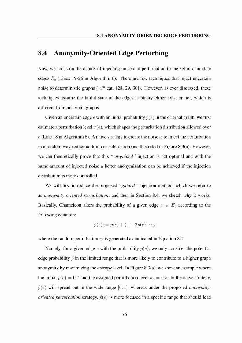
8.4 ANONYMITY-ORIENTED EDGE PERTURBING
8.4 Anonymity-Oriented Edge Perturbing
Now, we focus on the details of injecting noise and perturbation to the set of candidate
edges Ec (Lines 19-26 in Algorithm 6). There are few techniques that inject uncertain
noise to deterministic graphs ( 4th cat. [28, 29, 30]). However, as ever discussed, these
techniques assume the initial state of the edges is binary either exist or not, which is
different from uncertain graphs.
Given an uncertain edge ewith an initial probability p(e) in the original graph, we first
estimate a perturbation level σ(e), which shapes the perturbation distribution allowed over
e (Line 18 in Algorithm 6). A naive strategy to create the noise is to inject the perturbation
in a random way (either addition or subtraction) as illustrated in Figure 8.3(a). However,
we can theoretically prove that this “un-guided” injection is not optimal and with the
same amount of injected noise a better anonymization can be achieved if the injection
distribution is more controlled.
We will first introduce the proposed “guided” injection method, which we refer to
as anonymity-oriented perturbation, and then in Section 8.4, we sketch why it works.
Basically, Chameleon alters the probability of a given edge e ∈ Ec according to the
following equation:
p(e) := p(e) + (1− 2p(e)) · re
where the random perturbation re is generated as indicated in Equation 8.1
Namely, for a given edge e with the probability p(e), we only consider the potential
edge probability p in the limited range that is more likely to contribute to a higher graph
anonymity by maximizing the entropy level. In Figure 8.3(a), we show an example where
the initial p(e) = 0.7 and the assigned perturbation level σe = 0.5. In the naive strategy,
p(e) will spread out in the wide range [0, 1], whereas under the proposed anonymity-
oriented perturbation strategy, p(e) is more focused in a specific range that should lead
76

8.4 ANONYMITY-ORIENTED EDGE PERTURBING
(a) (b)
Figure 8.3: Chameleon: Anonymity-Oriented Edge Perturbation.
to a higher entropy.
Clearly, existing schemes in literature—which are defined over deterministic graphs—
become a special case of the proposed scheme (by setting p(e) to either 0 or 1).
Proof Sketching the Heuristic
We proceed to elaborate the rationality this anonymity-oriented edge perturbing scheme
briefly. The formal detail proof of our heuristic is available in tech report. The core idea
is to maximize the entropy of degree uncertainty matrix (referred to as ME).
To facilitate further discussion, we consider the extreme case k-obf, which poses a
set of hard constraints over the anonymized solution. Let the constraint being k-obf be
C, k−obfuscate a vertex v be cv. According to Definition 8, k−obf can be expressed as
joint satisfaction of cv : v ∈ V since the uncertain graph is said to be k-obf iff it
k−obfuscates all the vertices. The formal definition as follows.
C =∏v∈V
cv (8.2)
77

8.4 ANONYMITY-ORIENTED EDGE PERTURBING
where
cv :=
1 H(YP (v)) ≥ log2 k
0 otherwise
In other words, given an uncertain graph, its satisfaction evaluation of C indicates whether
it achieves the desirable anonymity level (k-obf).
However, as shown in Figure 8.3(b), a single constraint at the vertex level is either
fully satisfied or fully violated. It limits the optimization opportunity of methods based
on local search. In this work, we model the individual constraint cv to a fuzzy relation in
which the satisfaction of a constraint is a continuous function of its variables’ values (i.e.,
the entropy H(YP (v)), going from fully satisfied to fully violated as follows.
Cv = eH(YP (v))−log2 |V | (8.3)
Theorem 7 Let Ω presents the domain of degree values in the original uncertain graph,
the maximization of the provided anonymity C is equivalent to the maximization of the
following function: ∑ω∈Ω
s(ω) ·H(Yω) (8.4)
Proof Sketch: First we can see that
C =∏v∈V
cv =∏ω∈Ω
cω . . . cω︸ ︷︷ ︸s(ω)
Taking logarithm for both sides and combining with the approximation equation 8.3, we
78

8.4 ANONYMITY-ORIENTED EDGE PERTURBING
can see that
log(C) =∑ω∈Ω
s(ω) log(cω)
=∑ω∈Ω
s(ω)[H(Yω)− log2 |V |
]=∑ω∈Ω
s(ω)H(Yω)−∑ω∈Ω
log2 |V |
Therefore, after removing the constant∑
ω log2 |V | from log(C), our goal is actually to
maximize Equation 8.4. It provides us with the relation between the global anonymity
and the level of disorder of the degree uncertainty matrix.
Theorem 8 The maximization of Equation 8.4 is equivalent to maximization of the fol-
lowing function:
∑ω∈Ω
s(ω) ·H(Yω) =[∑v∈V
H(dv)]
+ |V | log |V | − |V |H(Ω) (8.5)
The equation stems from the coding length of degree uncertainty matrix from different
perspectives (row and column).1
It provides us with the mechanism for gaining better anonymity, namely increasing the
degree uncertainty per vertex H(dv).
Theorem 9 As implied by the Central Limit Theorem, dv may be approximated by the
normal distribution N(µ, σ2), where µ =∑
e∈Ev p(e) and σ2 =∑
e∈Ev p(e) − p(e)2.
Therefore, its entropy may be approximated by the differential entropy of the normal dis-
tribution 12
ln(2πσ2)+ 12. For a given p(e), its gradient ascent is proportion to 1−2 ·p(e).
Targeting at high entropy, we apply the gradient ascent method—p(e) = p(e) +(1 − 2 ·
p(e))· re for achieving the increase of degree entropy and the anonymity gain.
1More detail of it is available in tech report.
79

8.4 ANONYMITY-ORIENTED EDGE PERTURBING
Proof
We consider the case that a vertex can be re-identified by its degree in the context of
uncertain graphs. Given a uncertain graph G = (V,E, p), let Xωv presents the probability
that a node v with degree value ω over all the possible worlds, and s(ω) presents the
expected number of nodes with degree value ω over the vertices in G. According to the
expectation sum rule, we know,
s(ω) :=∑v∈V
Xωv
Let Yvω presents the probability that a node v is the image of the target node has degree
value ω. Yω corresponds to the posterior probability of the node v given the evidence
degree value ω. Based on the Bayesian theorem, we get the following equation,
Yvω :=Xv(ω)
s(ω)
Accordingly, the entropy of the distribution Yω over the vertices of G is defined as follows.
H(Y (ω)) =∑v
−1 · Yvω log Yvω
=∑v
−1 · Xv(ω)
s(ω)log
Xv(ω)
s(ω)
=∑v
−1 · Xv(ω)
s(ω)[logXv(ω)− log s(ω)]
=∑v
log s(ω) · Xv(ω)
s(ω)+∑v
−1 · Xv(ω)
s(ω)logXv(ω)
= log s(ω) +1
s(ω)·∑v
−1 · Xv(ω) logXωv
80

8.4 ANONYMITY-ORIENTED EDGE PERTURBING
Thus, we get the concise expression of weighted entropy sum as follows.
∑ω
s(ω)H(Y (ω)) =∑ω
s(ω) log s(ω) +∑ω
∑v
−1 · Xωv logXω
v
=∑ω
s(ω) log s(ω) +∑v
∑ω
−1 · Xωv logXω
v︸ ︷︷ ︸Switch Order
=∑ω
s(ω) log s(ω) +∑v
−1 · Xωv logXω
v︸ ︷︷ ︸Entropy
=∑ω
s(ω) log s(ω) +∑v
H(v)
=∑ω
n · Pω log nPω +∑v
H(v)
=n log n− nH(Ω) +∑v
H(v)
Where H(v) represents the entropy of probability distribution of a given node v’s degree,
H(Ω) represents the entropy of probability distribution regarding to the degree distribu-
tion of the overall uncertain graph. To further simply our problem, we assume the global
degree distribution holds constant in the anonymization process or with little change.
Fix v ∈ G and let e1, ·, el be l edges that involve v. For each 1 ≤ i ≤ l, ei is Bernoulli
random variable that equals 1 with some probability p. Let dv be the random variable
corresponding to the degree of v, we have
dv =l∑
i=1
ei
Since dv is the sum of independent random variable, it may be approximated by the
normal distribution N(µ, σ2), where µ =∑E(ei) =
∑pi and σ2 =
∑V ar(ei) =∑
pi(1 − p(i)) as implied by Central Limit Theorem (in the case l ≈ 30; for typical
sizes of l in uncertain graphs, the normal approximation becomes very accurate). Recall
81

8.4 ANONYMITY-ORIENTED EDGE PERTURBING
that, uncertain graph anonymization techniques focus on modifying the less anonymized
nodes. Usually, they are nodes with high degree. This approximation is reasonable. Fol-
lowing this path, H(v) can be approximated as the differential entropy of the normal
distribution.H =− g(x) ln g(x)
=−∫
1√2πσ2
e(x−µ)2
2σ2 ln[1√
2πσ2e
(x−µ)2
2σ2 ]
=1
2ln(2πeσ2)
On this basis, we can get the partial derivative of the weighted entropy sum with respect
to the uncertainty associated to a specific edge e = (u, v) as
∂C(G)
∂p(e)=∂[H(v) +H(u)]
∂p(e)
=∂H(v)
∂σ2v
· σ2v
∂p(e)+∂H(u)
∂σ2u
· σ2u
∂p(e)
∝ 1− 2p(e)
Where we assume the global degree distribution has been changed little, i.e., H(Ω) is
constant.
82

9
Performance Evaluation
Extensive experiments are conducted to evaluate the effectiveness and efficiency of un-
certain graph anonymization methods as summarized in Table 9.2.
9.1 Experiment Settings
9.1.1 Data Collection
We tested our algorithm on three real-world uncertain graph datasets. The characteristics
of these datasets are summarized in Table 13.1.
• DBLP1 is a dataset of scientific publications and authors. In this dataset, each node
represent an author. Two authors are connected by an edge if they have co-authored in
a project. The uncertainty on the edge denotes the probability that the two authors will
collaborate in a new project. It is obtained by a predictive model based on historical data
as described in the literature [28, 68]. The larger the number of coauthored papers, the
more likely they collaborate in a new project.
• Brightkite2 is a location-based social network. In this dataset, each node represent a1http://dblp.dagstuhl.de/xml/release/dblp-2015-11-012https://snap.stanford.edu/data/loc-brightkite.html
83
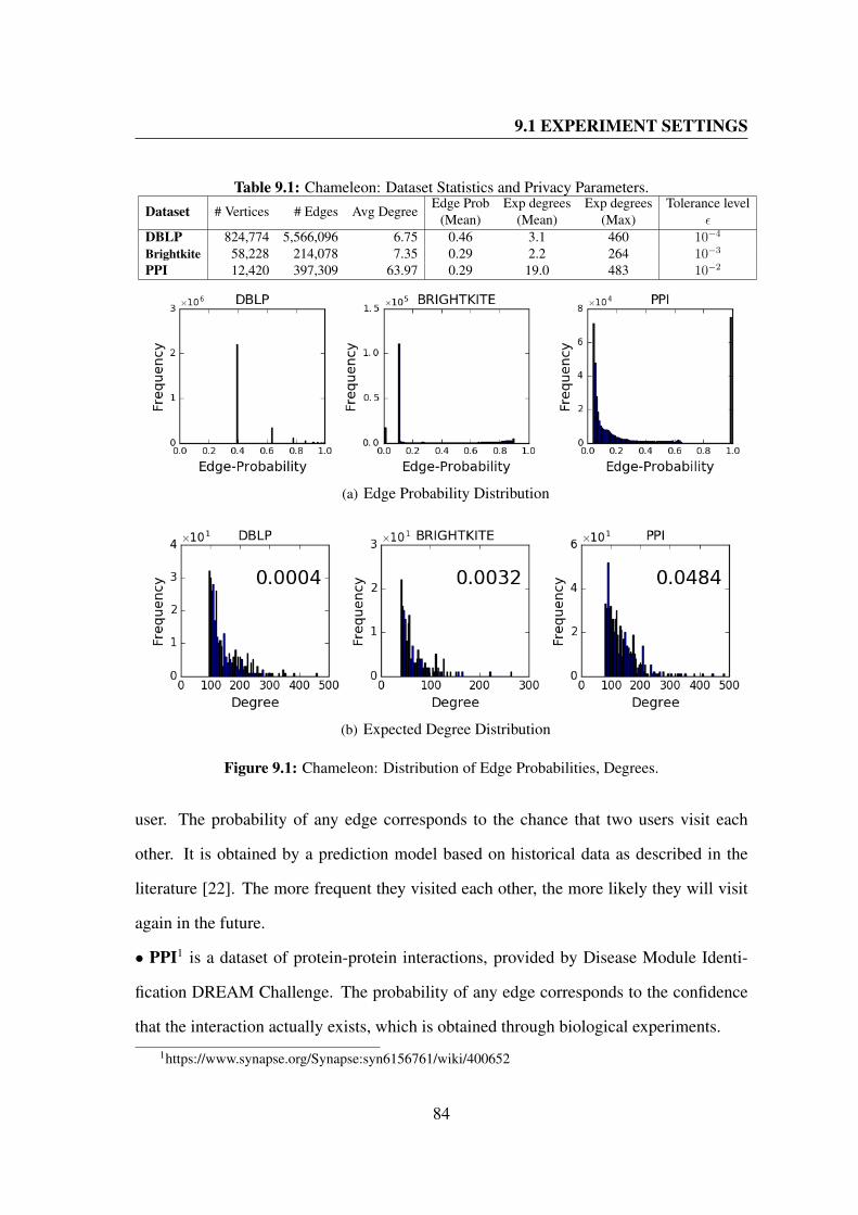
9.1 EXPERIMENT SETTINGS
Table 9.1: Chameleon: Dataset Statistics and Privacy Parameters.Dataset # Vertices # Edges Avg Degree
Edge Prob(Mean)
Exp degrees(Mean)
Exp degrees(Max)
Tolerance levelε
DBLP 824,774 5,566,096 6.75 0.46 3.1 460 10−4
Brightkite 58,228 214,078 7.35 0.29 2.2 264 10−3
PPI 12,420 397,309 63.97 0.29 19.0 483 10−2
(a) Edge Probability Distribution
(b) Expected Degree Distribution
Figure 9.1: Chameleon: Distribution of Edge Probabilities, Degrees.
user. The probability of any edge corresponds to the chance that two users visit each
other. It is obtained by a prediction model based on historical data as described in the
literature [22]. The more frequent they visited each other, the more likely they will visit
again in the future.
• PPI1 is a dataset of protein-protein interactions, provided by Disease Module Identi-
fication DREAM Challenge. The probability of any edge corresponds to the confidence
that the interaction actually exists, which is obtained through biological experiments.
1https://www.synapse.org/Synapse:syn6156761/wiki/400652
84

9.1 EXPERIMENT SETTINGS
Figure 9.1(a) shows the edge-probability distribution in the three datasets. Note that
the DBLP dataset only has a few probability values, while Brightkite dataset’s proba-
bility values are generally very small. The PPI dataset has a more uniform probability
distribution. We also present their degree distributions of “unique” nodes (with high de-
gree and obfuscation level is smaller than 300). Observe that, all the three graphs have a
heavy-tailed degree distribution,namely, they are difficult to be anonymized.
9.1.2 Evaluation Metrics
The primary goal is to preserve the utility of an anonymized graph in a high level. There-
fore, we measure the utility of uncertain graphs in terms of general structural properties,
i.e., degree-based statistics, shortest-distance statistics, and clustering statistics, following
the existing literature [28, 30].
Degree-based statistics
• Number of edges : SNE = 12
∑v∈V dv
• Average degree: SAD = 1n
∑v∈V dv
• Maximal degree: SMD = maxv∈V dv
• Degree variance: SDV = 1n
∑v(dv − SAD)2
• Power-law exponent of degree sequence: SPL is the estimate of γ assuming the
degree sequence follows a power-law4(d) ≈ d−γ
Shortest path-based statistics
• Average distance: SAPD is the average distance among all pairs of vertices that are
path-connected.
• Effective diameter: SED is the 90-th percentile distance among all all path-connected
pairs of vertices.
85
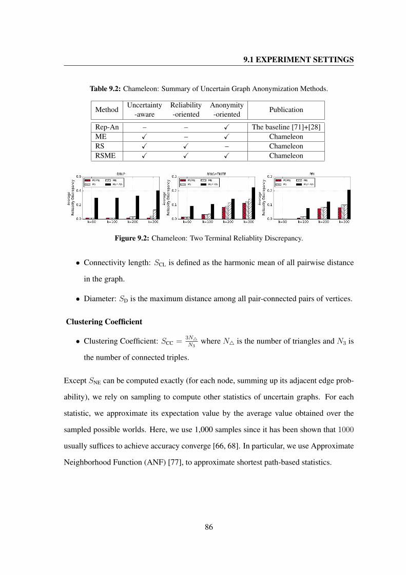
9.1 EXPERIMENT SETTINGS
Table 9.2: Chameleon: Summary of Uncertain Graph Anonymization Methods.
MethodUncertainty
-awareReliability-oriented
Anonymity-oriented
Publication
Rep-An – – X The baseline [71]+[28]ME X – X ChameleonRS X X – ChameleonRSME X X X Chameleon
Figure 9.2: Chameleon: Two Terminal Reliablity Discrepancy.
• Connectivity length: SCL is defined as the harmonic mean of all pairwise distance
in the graph.
• Diameter: SD is the maximum distance among all pair-connected pairs of vertices.
Clustering Coefficient
• Clustering Coefficient: SCC =3N4N3
where N4 is the number of triangles and N3 is
the number of connected triples.
Except SNE can be computed exactly (for each node, summing up its adjacent edge prob-
ability), we rely on sampling to compute other statistics of uncertain graphs. For each
statistic, we approximate its expectation value by the average value obtained over the
sampled possible worlds. Here, we use 1,000 samples since it has been shown that 1000
usually suffices to achieve accuracy converge [66, 68]. In particular, we use Approximate
Neighborhood Function (ANF) [77], to approximate shortest path-based statistics.
86

9.2 PERFORMANCE OF UNCERTAIN GRAPH ANONYMIZATION
(a) Brighte dataset (b) PPI dataset
Figure 9.3: Chameleon: Running Time Comparision vs. Rep-An.
9.2 Performance of Uncertain Graph Anonymization
9.2.1 Efficiency Evaluation
In the first set of experiments, we consider four obfuscation levels, k ∈ 60, 100, 200, 300,
and tolerance levels ε presented in Table 13.1. We experimented with the setting: white
noise level q = 0.01, obfuscation attempt t = 5, and initial size multiplier c = 1.3. In
some cases, anonymization algorithms failed to find a proper upper bound for σ in the
loop. In those cases, we increase the size multiplier c.
These obfuscation algorithms were implemented in C++ and run on Intel Core i7
CPU, 2 GHZ, 6MB cache size. We report their computation time on PPI and Brightkite
dataset in Figure 13.1. Note that, the PPI is already (60, 0.01)-obfuscated, thus no
anonymization effort is needed. For a larger values for anonymity level k, it takes long
time to output (k, ε)-obf as shown in Figure 13.1(c). It is because the increased efforts
(larger size multiplier c for a more significant amount of noise) needed to achieve the
higher obfuscation level (larger values of k).
In general, the time efficiency of our Chameleon approaches is close to the Rep-An
approach. For the small values of anonymity level k, the efficiency of the three Chameleon
variants is similar. For the larger values of k, RSME is faster than RS and ME. This
is because the combination of reliability sensitive edge selection scheme (RS) and max
87

9.2 PERFORMANCE OF UNCERTAIN GRAPH ANONYMIZATION
Figure 9.4: Chameleon: Graph Property Preservation.
entropy based edge perturbation scheme (ME) has the benefit of maximizing obfuscation
effect with the same noise budget, and keeping the graph size under control, namely, the
smaller size multiplier c. Smaller values of c reduce the running time of Algorithm 7,
where the main loop is over c|E| edges. This effect is evident in Figure 13.1(c), where
the time performance of RSME substantially is better than others.
9.2.2 Utility Loss
To assess how anonymization impacts utility, we compare the anonymized output to the
original uncertain graph based on aforementioned important graph properties. For each
property, we measure it on the original graph and on the anonymized output using the
sampling method. We report the difference of their expectation values.
Reliability Preserving In particular, we report the average reliability discrepancy of
anonymized graphs in Figure 9.2. The smaller discrepancy, the better the reliability pre-
serving, the better graph structure preserving. In all cases, the RSME approach performs
88
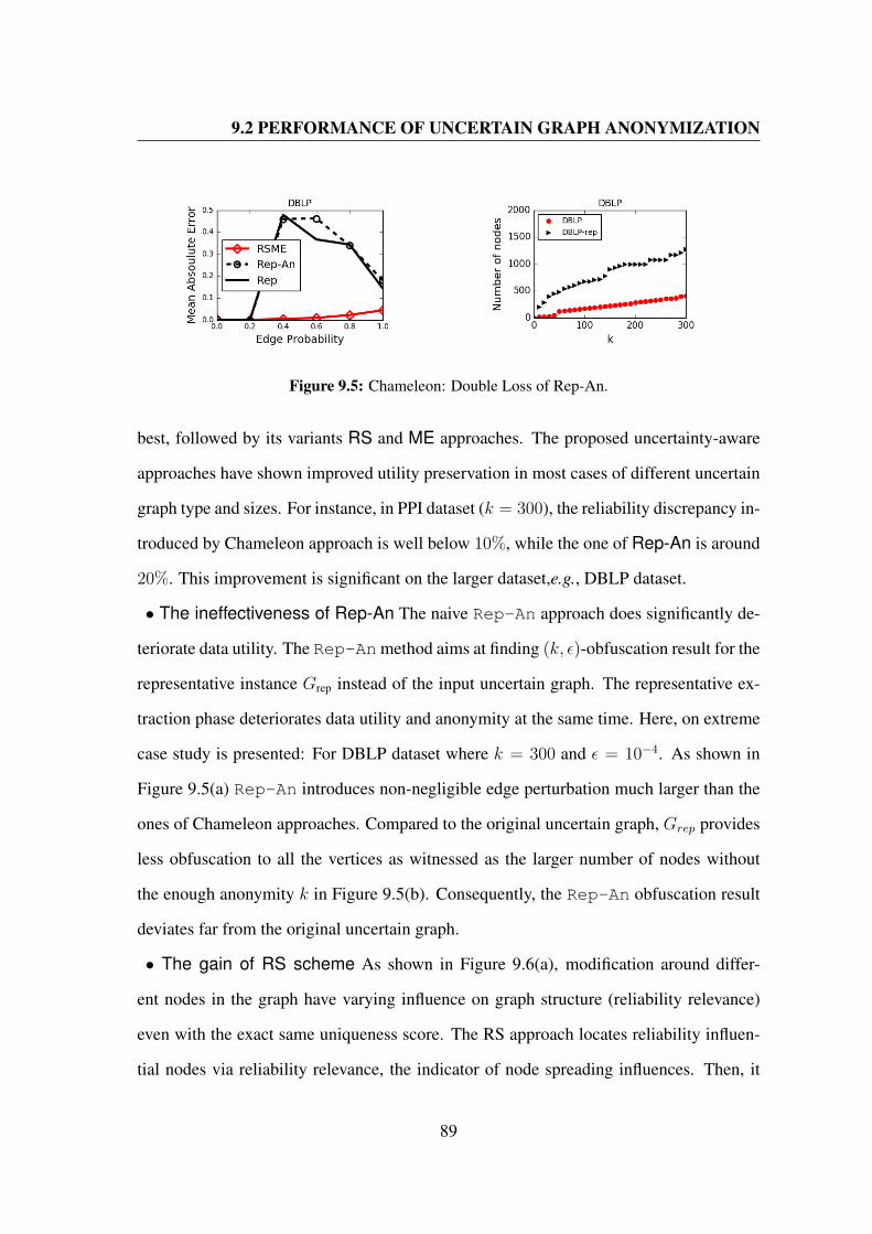
9.2 PERFORMANCE OF UNCERTAIN GRAPH ANONYMIZATION
Figure 9.5: Chameleon: Double Loss of Rep-An.
best, followed by its variants RS and ME approaches. The proposed uncertainty-aware
approaches have shown improved utility preservation in most cases of different uncertain
graph type and sizes. For instance, in PPI dataset (k = 300), the reliability discrepancy in-
troduced by Chameleon approach is well below 10%, while the one of Rep-An is around
20%. This improvement is significant on the larger dataset,e.g., DBLP dataset.
• The ineffectiveness of Rep-An The naive Rep-An approach does significantly de-
teriorate data utility. The Rep-Anmethod aims at finding (k, ε)-obfuscation result for the
representative instance Grep instead of the input uncertain graph. The representative ex-
traction phase deteriorates data utility and anonymity at the same time. Here, on extreme
case study is presented: For DBLP dataset where k = 300 and ε = 10−4. As shown in
Figure 9.5(a) Rep-An introduces non-negligible edge perturbation much larger than the
ones of Chameleon approaches. Compared to the original uncertain graph, Grep provides
less obfuscation to all the vertices as witnessed as the larger number of nodes without
the enough anonymity k in Figure 9.5(b). Consequently, the Rep-An obfuscation result
deviates far from the original uncertain graph.
• The gain of RS scheme As shown in Figure 9.6(a), modification around differ-
ent nodes in the graph have varying influence on graph structure (reliability relevance)
even with the exact same uniqueness score. The RS approach locates reliability influen-
tial nodes via reliability relevance, the indicator of node spreading influences. Then, it
89

9.2 PERFORMANCE OF UNCERTAIN GRAPH ANONYMIZATION
(a) RSME vs. ME (b) RSME vs. RS
Figure 9.6: Chameleon: The Gain of RS and ME.
prevents edges connected with such influential nodes from larger modification. By re-
strictive preserving the graph skeleton, the RSME scheme is able to preserve the essence
of the original uncertain graph.
• The gain of ME scheme The generic anonymization approach alters the probabil-
ity values associated with selected edges randomly. For each anonymization attempt, it
fails to guarantee the increase of provided anonymity. Therefore, it requires more noise
than the RSME which adopts the max-entropy principle for guiding edge alteration. Fig-
ure 9.6(b) shows the RS approach introduces larger noises to edge probability compared
to the RSME and ME approaches.
Other statistics Preserving For other statistics, we computed the average statistical
error, that is, the relative absolute difference between the estimation and the real value.
The smaller error, the better utility preserving. We present three statistics comparison in
Figure 9.4.
In general, the RSME can better preserve graph properties such degree, distance, and
clustering coefficient as shown as smaller errors in Figure 9.4. Conversely, for small
values of k, e.g., k = 60, errors introduced by Chameleon approaches are always smaller
than 1%. The larger values of k, the larger errors introduced. The RSME approach keeps
the error in control, better than the other, up to 12% in the PPI dataset. Such benefit is of
particular importance for large networks, e.g., DBLP dataset. We observed that the use of
90

9.2 PERFORMANCE OF UNCERTAIN GRAPH ANONYMIZATION
RS strategy also better preserves uncertain graph structures, as witnessed as small errors
in average path length and clustering coefficient. We attribute this phenomenon to that the
strong relation between the reliability (connectivity) and the path distance property. The
reliability sensitive edge selection strategy (RS) avoids injecting noise over influential
nodes (in the structural context). Thus, it can preserve the uncertain graph structure, as
witnessed as better performance in Figure 9.4.
Summary
Therefore, we can safely conclude that our experimental assessment on real-world
datasets confirms the initial and driving intuition: the Chameleon approach which explic-
itly incorporates edge uncertainty and the possible world semantic in the anonymization
process outperforms the baseline Rep-An approach significantly regarding the uncertain
graph utility preservation. And, the efficiency of the Chameleon approach is similar to
the one of the Rep-An approach.
Another message is: by using fine-grained and uncertainty-aware perturbation strate-
gies such as reliability sensitive edge selection (RS) and max entropy based edge prob
alteration (ME), one can achieve the same desired level of obfuscation with the smaller
change on the uncertain graph thus maintaining higher data utility.
91

10
Related Work
Privacy Attack Models on Graph Data: The assumptions of the adversary knowledge
K—which represent the types of prior knowledge that an adversary may attain and utilize
for graph de-anonymization—play a critical role in modeling privacy attacks and develop-
ing anonymization approaches. For un-weighted graphs, the common types of adversary
knowledge K includes attributes of vertices, links between some target individuals, vertex
degree, neighborhood, embedded subgraphs, and graph metrics (e.g., betweenness, close-
ness, centrality) [48]. For weighted graphs, edge weights are considered to be the most
common adversary knowledge. Table 10.1 summarizes the existing graph anonymization
techniques w.r.t their assumptions of adversary knowledge. As can be observed, vertex
degree, where the adversary is assumed to have knowledge about the nodes’ degrees, is
the most common attack model.
Deterministic Graph Anonymization: Existing graph anonymization approaches
are tailored to deterministic graphs (unweighted & weighted). The majority of them fo-
cuses on un-weighted deterministic graphs. These approaches can be classified into
four categories: (1) Clustering-based generalization [48, 49, 69, 73, 74, 78], (2) Edge
modification [27, 43, 44, 54, 72, 79, 80], (3) Edge randomization [31, 32, 33, 34], and
92
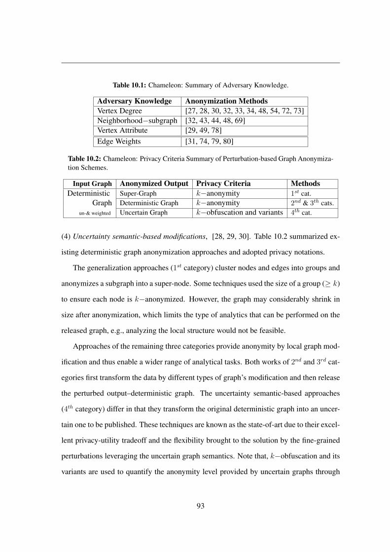
Table 10.1: Chameleon: Summary of Adversary Knowledge.
Adversary Knowledge Anonymization MethodsVertex Degree [27, 28, 30, 32, 33, 34, 48, 54, 72, 73]Neighborhood−subgraph [32, 43, 44, 48, 69]Vertex Attribute [29, 49, 78]Edge Weights [31, 74, 79, 80]
Table 10.2: Chameleon: Privacy Criteria Summary of Perturbation-based Graph Anonymiza-tion Schemes.
Input Graph Anonymized Output Privacy Criteria MethodsDeterministic Super-Graph k−anonymity 1st cat.
Graph Deterministic Graph k−anonymity 2nd & 3th cats.un-& weighted Uncertain Graph k−obfuscation and variants 4th cat.
(4) Uncertainty semantic-based modifications, [28, 29, 30]. Table 10.2 summarized ex-
isting deterministic graph anonymization approaches and adopted privacy notations.
The generalization approaches (1st category) cluster nodes and edges into groups and
anonymizes a subgraph into a super-node. Some techniques used the size of a group (≥ k)
to ensure each node is k−anonymized. However, the graph may considerably shrink in
size after anonymization, which limits the type of analytics that can be performed on the
released graph, e.g., analyzing the local structure would not be feasible.
Approaches of the remaining three categories provide anonymity by local graph mod-
ification and thus enable a wider range of analytical tasks. Both works of 2nd and 3rd cat-
egories first transform the data by different types of graph’s modification and then release
the perturbed output–deterministic graph. The uncertainty semantic-based approaches
(4th category) differ in that they transform the original deterministic graph into an uncer-
tain one to be published. These techniques are known as the state-of-art due to their excel-
lent privacy-utility tradeoff and the flexibility brought to the solution by the fine-grained
perturbations leveraging the uncertain graph semantics. Note that, k−obfuscation and its
variants are used to quantify the anonymity level provided by uncertain graphs through
93
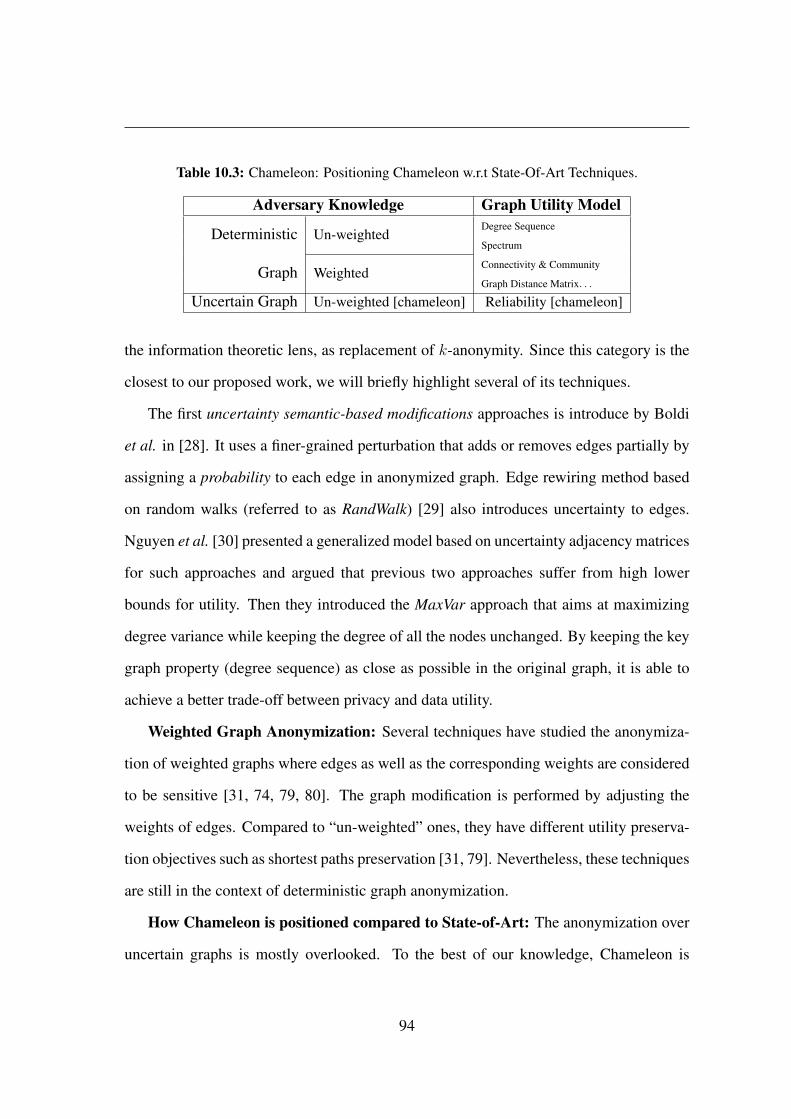
Table 10.3: Chameleon: Positioning Chameleon w.r.t State-Of-Art Techniques.
Adversary Knowledge Graph Utility Model
Deterministic Un-weightedDegree Sequence
Spectrum
Graph WeightedConnectivity & Community
Graph Distance Matrix. . .
Uncertain Graph Un-weighted [chameleon] Reliability [chameleon]
the information theoretic lens, as replacement of k-anonymity. Since this category is the
closest to our proposed work, we will briefly highlight several of its techniques.
The first uncertainty semantic-based modifications approaches is introduce by Boldi
et al. in [28]. It uses a finer-grained perturbation that adds or removes edges partially by
assigning a probability to each edge in anonymized graph. Edge rewiring method based
on random walks (referred to as RandWalk) [29] also introduces uncertainty to edges.
Nguyen et al. [30] presented a generalized model based on uncertainty adjacency matrices
for such approaches and argued that previous two approaches suffer from high lower
bounds for utility. Then they introduced the MaxVar approach that aims at maximizing
degree variance while keeping the degree of all the nodes unchanged. By keeping the key
graph property (degree sequence) as close as possible in the original graph, it is able to
achieve a better trade-off between privacy and data utility.
Weighted Graph Anonymization: Several techniques have studied the anonymiza-
tion of weighted graphs where edges as well as the corresponding weights are considered
to be sensitive [31, 74, 79, 80]. The graph modification is performed by adjusting the
weights of edges. Compared to “un-weighted” ones, they have different utility preserva-
tion objectives such as shortest paths preservation [31, 79]. Nevertheless, these techniques
are still in the context of deterministic graph anonymization.
How Chameleon is positioned compared to State-of-Art: The anonymization over
uncertain graphs is mostly overlooked. To the best of our knowledge, Chameleon is
94

the first anonymization framework in that context. Compared to all existing techniques,
we address a different input graph model—which is the uncertain model. Compared to
weighted graphs, uncertain graphs represent an entirely different model with different
semantics and possible analytics [66]. Basically, “weighted” and “uncertain” are two
orthogonal properties of a graph, i.e., an uncertain graph (where edges have real-world
presence probabilities) can be either weighted (where an edge has a weight (if present)) or
un-weighted. It has been discussed in [66] that casting an uncertain graph to a weighted
graph—with the goal of leveraging existing analytical techniques—leads to an incorrect
semantics. Evidently, the same applies to the anonymization problem at hand. Thus,
existing techniques for weighted deterministic graphs [31, 74, 79, 80] cannot be applied
to un-weighted uncertain graphs.
Chameleon falls under the 4th category mentioned above (Uncertainty semantic-based
modifications) since it consumes and produces graphs of uncertain type. Conceptually,
various attack models and privacy criteria can be considered—the uncertain graph model
can even trigger new attack models that were not applicable in the context of deterministic
graphs. However, as a starting point, we focus on the vertex-degree (a.k.a degree-based)
attack model [27] as one of the most serious and common models combined with the
k-obfuscation privacy criteria as the most suitable for uncertain graphs as shown in Ta-
ble 10.2.
95
Part III
Resisting Probabilistic Degree-based
De-anonymization in Anonymized
Uncertain Graphs
96
11
Problem Definition
In this section, we describe the capabilities and motivations of the adversary in the context
of uncertain graphs. First, we show how the adversary may attack naively anonymized
uncertain graph with uncertain local knowledge, then define node re-identification risk
and corresponding privacy condition.
11.1 Privacy Threats
Uncertain graphs have the similar privacy issue with deterministic graphs, i.e., the ad-
versary may have access to external information about the entities in the graph and their
relationship. The information may be obtained by the malicious actions or public re-
source. For example, in social network, the neighbor of victims can estimate the number
of his/her close friends. Formally, the adversary might gain a sequence of observation
about “the close friends of Ana”. Equipped with such information, he may be able to
reduce the uncertainty in victim de-anonymization and threaten the privacy of entities
(individuals, companies or sensors). For example, the first statement allows the adver-
sary to partially re-identify Ana: cand(Ana) = a, b, c, d. According to the similiarity
97

11.1 PRIVACY THREATS
between prior knowledge of the victim individual and candidates nodes in the released
uncertain graph w.r.t specific subgraph signature (here, degree distribution), candidates
will be assigned with different likelihood of being the image of the victim node.
Following the lecture, we model the adversary’s external information as degree knowl-
edge for the vertices of the original uncertain graph G. Fix a vertex v ∈ G and let
e1 . . . , en−1 be the n − 1 pairs of vertices that include v. In the uncertain graph, ei of
each edge is a Bernoulli random variable that equals 1 with some probability pi. Thus,
we denote the degree of v as the random variable dv as
dv =n−1∑i=1
ei (11.1)
Then for each possible degree value ω of v, we have Xv(ω) = Pr(dv = ω). Through-
out this paper, we assume the adversary has the comprehensive view of dv for the vertices
v ∈ G. As shown in Equation 11.1, there is inherent uncertainty in the adversary knowl-
edge of the target node.
An adversary attempts re-identification for a target node v by using dv to locate the
candidate set. Since Ga is published, the adversary can evaluate degree of the vertices
on Ga, looking for matches. Likewise, for any vertex va ∈ Ga, its degree evaluation
is also uncertain. In determinitic graphs, the candidate set of a target x is the vertices
with the exact matching property. In the uncertain graph’s case, the adversary knowledge
and public structural signature both are uncertain. Therefore, we propose the generlized
conecpt of fuzzy candidate set by capaturing the matching likelihood between two random
variables.
Definition 6 (Fuzzy Candidate Set under Degree) The fuzzy candidate set of target
node v ∈ G w.r.t degree is fcand(v) = (u, Pr(du = dv)) where u ∈ Ga. Namely, it en-
codes the information of candidate node and the equivalent confidence of such matching.
98

11.1 PRIVACY THREATS
a
b
d
e f
c0.8
0.2
0.5
0.7
0.9
0.1
(a) An anonymized uncertain graph
Ana
;
0.08
0.08
0.84
(b) Adversary knowledge
Figure 11.1: Galaxy: Probabilistic Degree-based De-anonymization.
Definition 7 (Fuzzy Equivalence) Two random variables du and dv are said to be equal,
if the event du−dv = 0 occurs with probability 1. Let Ω be the domain. The probability
of du = dv can calculate as follows
Pr(du = dv) =∑ω∈Ω
Pr(du = dv = ω)
=∑ω∈Ω
Pr(du = ω)Pr(dv = ω)
(11.2)
Example 1 Referring to the example graph in Figure 11.1, for the target Ana, the adver-
sary have the discrete distribution of dAna as shown in Figure 11.1(b) and fuzzy candidate
sets a, b, c, d, e.
With respect to degree, we may compute degree uncertainty matrices for a given uncertain
graph G as XG as
x11 x12 x13 . . . x1d
x21 x22 x23 . . . x2d
......
......
...
xn1 xn2 xn3 . . . xnd
Then, we can compute the fuzzy equivalence f(v;u) based on the product of the two
99
11.2 ANONYMITY MEASUREMENT
degree uncertainty matrices as
XGXGaT (11.3)
Those computed values would give the values of f(v;u) for all v ∈ V and u ∈ U .
Each row in this matrix corresponds to an original vertex v ∈ V and gives the related
probabilities f(v;u) for all u ∈ U . This matrix F enables us to compute the poster-belief
distribution Yv by normalizing the corresponding row in the matrix:
Yvi(uj) =Fi,j∑1≤l≤n
Fi,j, 1 ≤ i, j ≤ n. (11.4)
11.2 Anonymity Measurement
In order to provide privacy protection to the vertices in uncertain graphs, we should limit
the low-bound of the uncertainty that the adversary would have when he tries to locate
the image of the target individual. We choose (k, ε)-obf [28] as the privacy condition
for following reasons. First, k−obf [34] provides an entropy-based quantification of the
uncertainty in de-anonymization which is more suitable for measuring the anonymity
provided by uncertain graphs. Moreover, the introduction of tolerance parameter ε which
allows ignoring up to ε∗|V | nodes which may represent extreme unique nodes,e.g., Trump
in Twitter Network, whose obfuscation is almost impossible. The formal definition is
given as follows:
Definition 8 (k, ε)-obf [28] Let P be a vertex property (i.e., vertex degree dist in our
work), k ≥ 1 be a desired level of anonymity, and ε > 0 be a tolerance parameter. An
anonymized uncertain graph G is said to k-obfuscate a given vertex v ∈ G w.r.t P if the
entropy H() of the distribution of fuzzy equivalence Yv over the vertices of G is greater
than or equals to log2 k:
H(Yv) ≥ log2 k.
100
11.3 UTILITY PRESERVATION
The uncertain graph G is (k, ε)-obf w.r.t property P if it k-obfuscates at least (1 − ε)|V |
vertices in G.
11.3 Utility Preservation
Ideally, the anonymized graph should preserve the privacy with the smallest utility loss
for permitting meaningful analysis tasks. In uncertain graph anonymization process, we
target at preserving the reliability property of an given uncertain graph. This choice is
motivated by the observation that reliability forms the foundation of numerous uncertain
graph theoretic algorithms such as k−nearest neighbors[18, 66], shortest paths detect-
ing [23, 58]. Specifically, we use the two-terminal reliability difference to reflect the
impact of anonymization on uncertain graph structure(referred to as Reliability Discrep-
ancy). The formal defintion of reliablity discrepancy is available at Chapter 6.
11.4 Problem Statement
Given the above foundation, we can now formulate the addressed problem—resisting
probabilitic degree-based de-anonymization in anonymized uncertain graphs.
Problem 2 Uncertain Graph Probabilitic Degree Anonymization Given an uncertain
graph G = (V,E, p) and anonymization parameters k and ε, the objective is to find a
(k, ε)-obfuscated uncertain graph G = (V,E, p) with minimal ∆(G). That is:
argminG
∆(G)
Subject to G is (k, ε)− obf
101

11.4 PROBLEM STATEMENT
Figure 11.2: Galaxy: Illustration of Convex and Non-Convex Set.
Non-convex Optimization Problem As ever discribed, the problem of resisting prob-
abilitic degree de-anonymization over uncertain graph is an typical constraint optimiza-
tion problem. The general form of an optimization problem is to find some s∗ ∈ S such
that
f(s∗) = minf(s) : s ∈ S, (11.5)
for some feasible set S ⊂ Rn and an objective f(s) : Rn → R. We are interested in the
convexity of its optimization model. The convex optimization problems share the desir-
able properties: they can be solved quickly and reliably up to very large size—hundreds
of thousands of variables and constraints. However, we will show in general, the problem
of uncertain graph anonymization under (k, ε) privacy notation is a typical non-convex
optimization where the objective or any constraint are non-convex.
The optimization problem is called a convex optimization problem if S is a convex set
and f(x) is a convex function defined on Rn. We start with the defintion of a convex set:
Definition 9 Convex set A subset S ⊂ Rn is a convex set if
x, y ∈ S ⇒ λx+ (1− λ)y ∈ S (11.6)
for λ ∈ [0, 1].
Figure 11.2 shows a convex set and a non-convex set.
102

11.4 PROBLEM STATEMENT
An Original Graph Anonymous Graphs(4, 0.2) obf
G1
(4, 0.2) obfNot
a
b
d
e
c
a
b
d
e
ca
b
d
e
c
G2
a
b
d
e
c
0.50.5
0.5
G3
Figure 11.3: Galaxy: Invalidity of Being Convex Set.
Here, we will show that the solution space of (k, ε)-obf is a non-convex set by con-
strugood counter example. As shown in Figure 11.3, G1 and G2 both 4-obfuscate at least
(1 − 0.2) × 5 = 4 vertices in the original graph since they blend any nodes with only
one neighbor among 4 nodes b, c, d, e in anonymized graph . If (4, 0.2)-obfuscation
instances of the original graph S is a convex set. According to Definition 9, G3 should
be one instance of S since G = λG1 + (1 − λ)G2 where λ = 0.5. However, G3 fails to
4-obfuscated at least (1− 0.2)× 5 = 4 vertices in the original graph since the candidate
cand(degree = 1) = (b, 1), (c, 1), (d, 0.5), (e, 0.5) the entropy of its normalized distri-
bution clearly is smaller than log2 4. In summary, we prove the general (k, ε)-obfucations
of a given uncertain graph isn’t a convex set and the problem is a typical non-convex
optimization problem.
Such a problem may have multiple feasible regions and multiple locally optimal points
within each region. It can take time exponential in the number of variables and con-
straints to determine that a non-convex problem is infeasible, that the objective function
is unbounded, or that an optimal solution is the “global optimum” across all feasible re-
gions. In this work, we propose a sound framework to efficiently solve the uncertain
graph anonymization problem in a practical time.
103

12
Galaxy Techniques
After introcuing the privacy attack model and the adaptive information entropy based
anonymity measure, we are ready to present our Galaxy algorithm that tries to anonymize
a given uncertain graph via edge uncertainty operation with the utility loss as small as
possible. In the following, we first present the basic idea of Galaxy and then detail its main
component individually. Notice that although we only focus on degree anonymization
in this thesis, our appraoch is general and it is applicable to other k-obfsucation based
privacy protection schemes on uncertain graphs.
12.1 Overview of The Galaxy Approach
We propose a two-step approach for the Probabilistic Graph Anonymization problem as
shown in Figure 12.1. For an input uncertain graph G = (V,E, p) with degree sequence
d and user-defined priacy criteria parameters (k, ε), we proceed as follows:
1. First, starting from d, we construct a new probabilistic degree sequence da that is
(k, ε)-obf and such that the degree anonymization cost is minimized.
104
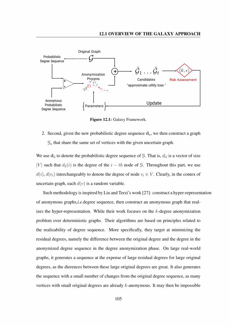
12.1 OVERVIEW OF THE GALAXY APPROACH
G+ G1 . . . GtAnonymization
Process Candidates“approximate utility loss ”
Original Graph
(k, )
Risk Assessment
Update Parameters
ProbabilisticDegree Sequence
AnonymousProbabilistic
Degree Sequence
+-
Figure 12.1: Galaxy Framework.
2. Second, given the new probabilistic degree sequence da, we then construct a graph
Ga that share the same set of vertices with the given uncertain graph.
We use dG to denote the probabilistic degree sequence of G. That is, dG is a vector of size
|V | such that dG(i) is the degree of the i − th node of G. Throughout this part, we use
d(i), d(vi) interchangeably to denote the degree of node vi ∈ V . Clearly, in the contex of
uncertain graph, each d(v) is a random variable.
Such methodology is inspired by Liu and Terzi’s work [27]: construct a hyper-representation
of anonymous graphs,i.e.degree sequence, then construct an anonymous graph that real-
izes the hyper-representation. While their work focuses on the k-degree anonymization
problem over deterministic graphs. Their algorithms are based on principles related to
the realizability of degree sequence. More specifically, they target at minimizing the
residual degrees, namely the difference between the original degree and the degree in the
anonymized degree sequence in the degree anonymization phase. On large real-world
graphs, it generates a sequence at the expense of large residual degrees for large original
degrees, as the dierences between these large original degrees are great. It also generates
the sequence with a small number of changes from the original degree sequence, as many
vertices with small original degrees are already k-anonymous. It may then be impossible
105

12.1 OVERVIEW OF THE GALAXY APPROACH
to compensate the large residual degrees. The sequence is then unrealizable. In summary,
the generated degree sequence may be not realizable. Probing scheme that operates small
random changes on the degree sequence util it is realizable and the graph is constructed.
However, the realizability testing has a time complexity O(|V |2) and Probing is invoked
for a large number of repetitions, the algorithm is very inefficient especially in the cases
of large graphs.
Our work differs in the address graph model and attack model—both are probabilistic.
Consequently, the output degree sequence of step 1 is also probabilistic. To the best of
our knowledge, the reliability of probabilistic degree sequence as the uncertain graph is
an unexplored problem.
Note that step 1 requires the anonymization cost of the probabilistic degree sequence
to be minimized, which in fact translated into the approximate requirement of the min-
imum changes. Step 2 tries to construct an uncertain graph with degree sequence da,
which is a supergraph (or has the large overlap in its sets of edges and edge probabilities)
with the original uncertain graph.
Considering the difficulty of obtaining the optimal solution that realizing the anony-
mous degree sequence, we consider the difficult of realizability in constructing probabilis-
tic (k, ε)-obf degree sequence. Inspired by the observation that the anonymous graph has
the large overlap in its set of edges and edge probabilities with the input uncertain graph,
instead of a Probing scheme, we construct the anonymized graph by operating modifi-
cation such as partial edge addition and deletion based on uncertainty semantic over the
given uncertain graph.
In the next sections, we develop algorithms for solving Probabilistic Degree Anonymiza-
tion Problem and Anonymous Graph Construction Problem.
106
12.2 PROBABILISTIC DEGREE ANONYMIZATION
12.2 Probabilistic Degree Anonymization
We give algorithms for solving the Probabilistic Degree Anonymization problem. Given
the probabilistic degree sequence d of the original input uncertain graph G = (V,E, p),
the algorithm output approximate solution of a (k, ε)-obf degree sequence da with the
minimal anonymization cost. We first show how to simplify the problem, then trans-
form it into a linear optimization problem. Then, we show how to derive the 1-Subgraph
perturbation plan on this basis.
Note that, k-obfuscation verification plays a major role in the uncertain graph anonymiza-
tion process. According to its definition, we need to compute degree uncertainty matrix
for a given perturbed uncertain graph Ga as XG, and verify k-obfuscation over the de-
rived the fuzzy equivalence matrix XGXGTa. Here, we will show the low bound based
k-obfuscation verifying.
Definition 10 An uncertain graph Ga = (V,Ea, pa) is (k, ε)-obf G if the probabilistic
degree sequence of Ga, is (k, ε)-obf the degree sequence of G.
Alternatively, Definition 10 that for every node v ∈ V in the input uncertain graph, the
entropy of the random variable Xv over U (a set of vertices in Ga) is at least logk. This
property prevents the re-identification of individuals by adversaries with a probabilis-
tic priori knowledge of the degree of specfic nodes. Together, the probabilistic degree
anonymization can expressed as
Problem 3 Probabilistic Degree Anonymization Given d, the probabilistic degree se-
quence of the given uncertain graph, and the privacy criteria (k, ε), constructed a (k, ε)-
obf sequence da with the minimal anonymization cost w.r.t degree sequence.
Note that, is a vector of random variables. As ever discussed, each dv can be approx-
imated by the normal distribution N(uv, σ2v) as implied by the Central Limit Theorem.
107
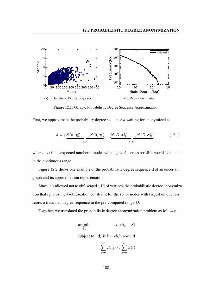
12.2 PROBABILISTIC DEGREE ANONYMIZATION
0 50 100 150 200 250 300 350 400
Mean
0
5
10
15
20
Std
dev
(a) Probabilistic Degree Sequence
100 101 102 103
Node Degree(log)
100
101
102
103
104
Frequency
(log)
Original
(b) Degree distribution
Figure 12.2: Galaxy: Probabilistic Degree Sequence Approximation.
First, we approximate the probability degree sequence d waiting for anonymized as
d = N(0, σ20), . . . , N(0, σ2
0)︸ ︷︷ ︸s(0)
. . . N(D, σ2D), . . . , N(D, σ2
D)︸ ︷︷ ︸s(D)
(12.1)
where s(i) is the expected number of nodes with degree i accross possible worlds, defined
in the continuous range.
Figure 12.2 shows one example of the probabilistic degree sequence d of an uncertain
graph and its approximation representation.
Since it is allowed not to obfuscated ε|V | of vertices, the probabilistic degree anonymiza-
tion that ignores the k-obfuscation constraint for the set of nodes with largest uniqueness
score, a truncated degree sequence in the pre-computed range D.
Together, we translated the probabilistic degree anonymization problem as follows:
argminSa
L1(Sa − S)
Subject to da is k − obfuscate dD∑i=0
Sa(i) <D∑i=0
S(i)
108
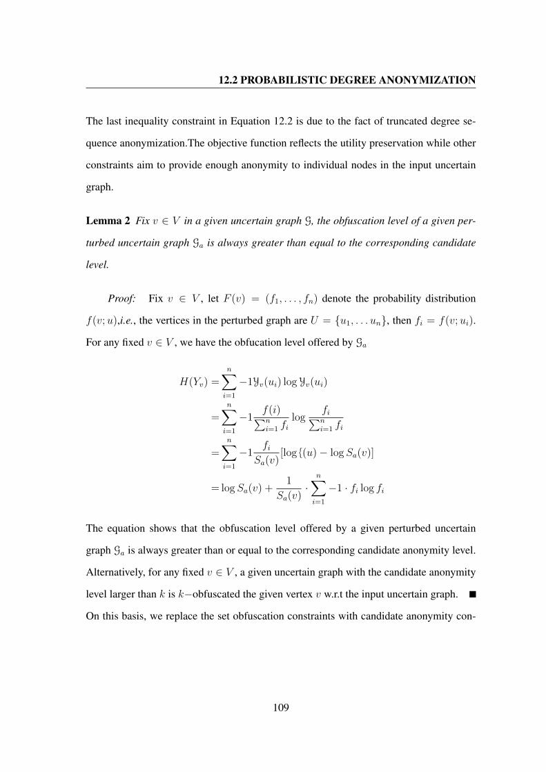
12.2 PROBABILISTIC DEGREE ANONYMIZATION
The last inequality constraint in Equation 12.2 is due to the fact of truncated degree se-
quence anonymization.The objective function reflects the utility preservation while other
constraints aim to provide enough anonymity to individual nodes in the input uncertain
graph.
Lemma 2 Fix v ∈ V in a given uncertain graph G, the obfuscation level of a given per-
turbed uncertain graph Ga is always greater than equal to the corresponding candidate
level.
Proof: Fix v ∈ V , let F (v) = (f1, . . . , fn) denote the probability distribution
f(v;u),i.e., the vertices in the perturbed graph are U = u1, . . . un, then fi = f(v;ui).
For any fixed v ∈ V , we have the obfucation level offered by Ga
H(Yv) =n∑i=1
−1Yv(ui) log Yv(ui)
=n∑i=1
−1f(i)∑ni=1 fi
logfi∑ni=1 fi
=n∑i=1
−1fi
Sa(v)[log (u)− logSa(v)]
= logSa(v) +1
Sa(v)·
n∑i=1
−1 · fi log fi
The equation shows that the obfuscation level offered by a given perturbed uncertain
graph Ga is always greater than or equal to the corresponding candidate anonymity level.
Alternatively, for any fixed v ∈ V , a given uncertain graph with the candidate anonymity
level larger than k is k−obfuscated the given vertex v w.r.t the input uncertain graph.
On this basis, we replace the set obfuscation constraints with candidate anonymity con-
109
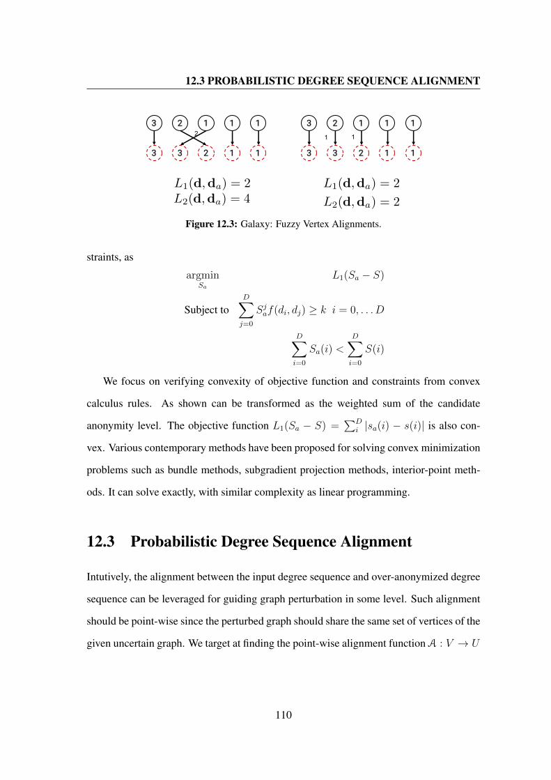
12.3 PROBABILISTIC DEGREE SEQUENCE ALIGNMENT
11123
11233
11123
11233
112
L1(d,da) = 2
L2(d,da) = 2
L1(d,da) = 2L2(d,da) = 4
Figure 12.3: Galaxy: Fuzzy Vertex Alignments.
straints, as
argminSa
L1(Sa − S)
Subject toD∑j=0
Sjaf(di, dj) ≥ k i = 0, . . . D
D∑i=0
Sa(i) <D∑i=0
S(i)
We focus on verifying convexity of objective function and constraints from convex
calculus rules. As shown can be transformed as the weighted sum of the candidate
anonymity level. The objective function L1(Sa − S) =∑D
i |sa(i) − s(i)| is also con-
vex. Various contemporary methods have been proposed for solving convex minimization
problems such as bundle methods, subgradient projection methods, interior-point meth-
ods. It can solve exactly, with similar complexity as linear programming.
12.3 Probabilistic Degree Sequence Alignment
Intutively, the alignment between the input degree sequence and over-anonymized degree
sequence can be leveraged for guiding graph perturbation in some level. Such alignment
should be point-wise since the perturbed graph should share the same set of vertices of the
given uncertain graph. We target at finding the point-wise alignment function A : V → U
110

12.3 PROBABILISTIC DEGREE SEQUENCE ALIGNMENT
with the minimal L2 distance w.r.t the original degree sequence:
∑v∈V
(d(v)− da(A(v)))2 (12.2)
The choice of such anonymization cost function stems from the observation that the diffi-
culty We show two alignments between the original degree sequence and the anonymous
one in Figure 12.3. L1 distance of the degree sequences corresponds to the number of
edge modifications. However, it can not distinguish two alignments. Clearly, L2 distance
prefers small and disperse edge additions around vertices. Without loss of generality, we
assume that entries in d and da are ordered in decreasing order of the degree expectations
they correspond to, that, d(1) ≥ d(1) ≥ . . . d(n). Let A be the optimal alignment solu-
tion w.r.t d and da, A(i) = i. Our experiments show that it performs extremely well in
practice.
Proof: Let A be any optimal alignment between d and a where A(i) = j, A(j) = i
and i < j. Then Let A′ be A except A′(i) = i, A′(j) = j. We have the anonymization
cost introduced by A
∑l∈[1,n]&l 6=i,j
[d(l)− da(l)]2 + [d(i)− da(j)]2 + [d(j)− da(i)]2
Likewise, the anonymization cost introduced by A′
∑l∈[1,n]&l 6=i,j
[d(l)− da(l)]2 + [d(i)− da(i)]2 + [d(j)− da(j)]2
111

12.4 PROBABLISTIC ANONYMOUS GRAPH CONSTRUCTION
1 3 13d = 3 d = 1d = 5
3 95
d = 3 d = 1d = 5
1 2 1 4 9Retention Rate: 9/13Variation Mean: 2Variation Stddev:0
Figure 12.4: Galaxy: Derived Perturbation Model.
We have their anonymization cost difference as
= [d(i)− da(j)]2 + [d(j)− da(i)]2 − [d(i)− da(i)]2 − [d(j)− da(j)]2
= [d(i)− d(j)][da(i)− da(j)]
≥ 0
This contradicts the assumption thatA is the optimal alignment solution with the minimal
L2 distance. Until here, we prove the greedy choice property of the alignment.
12.4 Probablistic Anonymous Graph Construction
It is tough to construct an uncertain graph from scratch that realizing the generated
probabilistic degree sequence. The previous works on deterministic graphs shows it is
computational expensive. Therefore, we turn to the other avenue that anonymizing un-
certain graphs by edge uncertainty perturbation under the anonymity bound. The main
idea of the algorithm is to utilize the over-anonymized degree sequence as the anonymity
bound of anonymization process.
For certain properties of interest, such as degree, the majority of vertices in real-world
graphs are already anonymous even without random perturbations. The reason is that
for most values of the property P there are many vertices have the same value. In other
words, their point-to-point distances over anonymous degree sequence are close to zero.
Hence, we aim at controlling the amount of applied perturbation, so that larger perturba-
112

12.5 THE ANONYMITY-BOUNDED OBFUSCATION ALGORITHM
Algorithm 8 Galaxy SkeletonInput: Uncertain graph G, adversary knowledge K, obfuscation level k, tolerancelevel ε, size multiplier c and white noise level qOutput: The anonymized result Gobf
1: da ← (k, ε)-obf(d)2: σl ← 0; σu ← 13: repeat4: 〈ε, G〉 ← galaxyObfuscation(G, k, ε, c, q, σu,K, da)5: if ε = 1 (fail) then σl ← σu; σu ← 2σu6: until ε 6= 17: repeat8: σ ← (σu + σl)/29: 〈ε, G〉 ← galaxyObfuscation(G, k, ε, c, q, σu,K, da)
10: if ε = 1 then σl ← σ11: else σu ← σ; Gobf ← G
12: until σu − σl is enough small13: return Gobf
tion is added at vertices with larger deviations. In particular, we suggest calibrating the
amount of perturbation applied to a vertex v according to its L1 distance w.r.t the matched
vertex as illustrated in Figure 12.4. To simulate stochastic degree sequence point-wise
matching, we calibrate retention rate and the deviation model as shown in Figure 12.4. In
particular, we suggest to the perturbation applied to a pair e = (u, v) ∈ Ec according to
the “distance” of the two vertices u and v w.r.t the anonymous image. Namely, if both
expected shift of v and u are small values, the re perturbation should be subtle; on the
other hand, v and u are inter-cluster matching nodes, then the perturbation re should be
higher. To mitigate the “mismatching” namely the expected shifts of u and v are in the
reverse direction, we adopt majority voting rule for deciding perturbation direction.
12.5 The Anonymity-Bounded Obfuscation Algorithm
Our algorithm for computing a (k, ε)-obf of an uncertain graph on the probabilistic node
degree is outlined as Algorithm 8. Note that, a (k, ε)-obf degree sequence provides
113

12.5 THE ANONYMITY-BOUNDED OBFUSCATION ALGORITHM
d = 3 d = 1d = 5
d = 5 d = 3 d = 1
v1 v2 v17
Figure 12.5: Galaxy: Anonymous Degree Sequence Realization.
high bound of anonymity guarantee. In other words, the obfuscation that exactly re-
alizes (k, ε)-obf degree sequence may suffer from high utility loss. Targeting for high
utility, our algorithm aims at injecting the minimal amount of noise needed to achieve
the require obfuscation. Likewise, computing the minimal amount of uncertainty is
achieved via a search on the anonymization parameters including size multiplier c and
the noise parameter σ. The search flow of Algorithm 8 is determined by the function
galaxyObfuscation, which is shown as Algorithm 9. Since the general iterative
skeleton is similar to Chameleon, we omit its detail here. The key difference between
Galaxy and Chameleon is the exploitation of (k, ε)-obf degree sequence in the function
galaxyObfuscation.
The function galaxyObfuscation (Algorithm 9) aims at finding a (k, ε)-obf of
G with given anonymization parameters (indicator of the total noise budget). Here, we
assume the utility loss is affected by the number of edge operations performed and the
utility loss caused by each edge operation. In other words, we try to solve the problem by
reducing the amount of noise and meanwhile perform the edge perturbations that cause
smaller utility with high priority. Intuitively, to align vertices with larger distance, a
larger amount of noise is necessary. Thus, edges need to be sampled with the higher
probability if they are adjacent to such vertices. To handle this sampling process, our
algorithm assigns a probabilityQ(v) to every v ∈ V , which is proportional to the expected
L1 distance w.r.t matched (k, ε)-obf degree sequence and the reverse to its reliability
114

12.5 THE ANONYMITY-BOUNDED OBFUSCATION ALGORITHM
Algorithm 9 GalaxyObfuscationInput: Uncertain graph G = (V,E, p), K, k, ε, c, q,standard deviation σ, and anonymous degree sequence daOutput: A pair 〈ε, G〉 where G is a (k, ε)−obfuscation, or ε = 1 if fail to find a(k, ε)-obf.
1: compute Average discrepancy ADv for v ∈ V2: compute the reliability relevance VRRv for v ∈ V3: Qv ← ADv · VRRv for v ∈ V4: H ← the set of d ε
2|V |e with largest Qv
5: Normalized VRRv for v ∈ V \H6: Qv ← ADv · 1− VRRv for v ∈ V \H7: ε← 18: for t times do9: RD ← targetedDiscrepancy(d, da)
10: repeat11: EC ← E12: randomly pick a vertex u ∈ V \H according to Q13: randomly pick a vertex v ∈ V \H according to Q14: if (u, v) ∈ E then15: EC ← Ec \ (u, v), TD[u], TD[v]+ = p(e), p(e) with the probability p(e)16: until EC = c|E|17: for all e ∈ EC do18: compute σ(e)19: draw w uniformly at random from [0, 1]20: if w < q then21: re ← U(0, 1)22: else23: re ← Rσ(e)
24: Inde ← majorityV oting(RD(u), RD(v))25: re = min(re, |RD(u)|, |RD(v)|)26: p(e) = p(e) + Inde · re27: RD(u)− = Inde · re; RD(v)− = Inde · re28: ε← anonymityCheck(G)
29: if ε < ε and ε then ε← ε; G← G
30: return 〈ε, G〉
centrality.
After that, the search for a (k, ε)-obf starts: the algorithm is randomized, and there is a
non-zero probability of failure, t attempts are executed. Each attempt begins by sampling
vertices matching as illustrated in Figure 12.5. Then, it starts by randomly selecting a
115

12.5 THE ANONYMITY-BOUNDED OBFUSCATION ALGORITHM
subsect of edges Ec, which will be subjected to edge perturbation where Ec is initialized
to E. The algorithm randomly select two distinct vertices u and v, according to the prob-
ability distribution Q. The edge (u, v) is removed from Ec with its existence probability
p(e), or added to Ec otherwise. Note that, the corresponding impact on node degree is
reflected in the pointwise perturbation bound. The process is repeated util EC reaches
the required size c|E|. The perturbation re-distribution process is similiar to Chameleon.
While, the amount of applied perturbation on specfic edge (u, v) is bounded by the resid-
ual perturbation of vertices u and v (Line 25).
116

13
Performance Evaluation
13.1 Experiment Settings
13.1.1 Data Collection
We tested our algorithm on three real-world uncertain graph datasets. The characteristics
of these datasets are summarized in Table 13.1.
• DBLP1 is a dataset of scientific publications and authors. In this dataset, each node
represent an author. Two authors are connected by an edge if they have co-authored in
a project. The uncertainty on the edge denotes the probability that the two authors will
collaborate in a new project.
• Brightkite2 is a location-based social network. In this dataset, each node represent a
user. The probability of any edge corresponds to the chance that two users visit each
other.
• PPI3 is a dataset of protein-protein interactions, provided by Disease Module Identi-
fication DREAM Challenge. The probability of any edge corresponds to the confidence
1http://dblp.dagstuhl.de/xml/release/dblp-2015-11-012https://snap.stanford.edu/data/loc-brightkite.html3https://www.synapse.org/Synapse:syn6156761/wiki/400652
117

13.1 EXPERIMENT SETTINGS
Table 13.1: Galaxy: Dataset Statistics and Privacy Parameters.
Dataset # Vertices # Edges Avg DegreeEdge Prob
(Mean)Exp degrees
(Mean)Exp degrees
(Max)Tolerance level
εDBLP 824,774 5,566,096 6.75 0.46 3.1 460 10−4
Brightkite 58,228 214,078 7.35 0.29 2.2 264 10−3
PPI 12,420 397,309 63.97 0.29 19.0 483 10−2
that the interaction actually exists, which is obtained through biological experiments.
13.1.2 Utility Evaluation
Measuring utility is hard as there is no standard metric to caputure it. An anonymization
scheme might perfectly preserve the degree distribution of a graph while damaging other
properties. Also, utility depends on the use of data by the analyst. As ever discussed.
reliablity plays a crticial role in uncertain graph analysis. Besides, we look at some fun-
damental utility metrics as they vary with anonymization level. The properties we study
are:
Degree-based statistics
• Number of edges : SNE = 12
∑v∈V dv
• Average degree: SAD = 1n
∑v∈V dv
• Maximal degree: SMD = maxv∈V dv
• Degree variance: SDV = 1n
∑v(dv − SAD)2
• Power-law exponent of degree sequence: SPL is the estimate of γ assuming the
degree sequence follows a power-law4(d) ≈ d−γ
They are used to capture the degree distribution which is an important measure of a small
world graph.
Shortest path-based statistics
• Average distance: SAPD is the average distance among all pairs of vertices that are
path-connected.
118

13.2 PERFORMANCE OF UNCERTAIN GRAPH ANONYMIZATION
• Effective diameter: SED is the 90-th percentile distance among all all path-connected
pairs of vertices.
• Connectivity length: SCL is defined as the harmonic mean of all pairwise distance
in the graph.
• Diameter: SD is the maximum distance among all pair-connected pairs of vertices.
Clustering Coefficient
• Clustering Coefficient: SCC =3N4N3
where N4 is the number of triangles and N3 is
the number of connected triples.
The clustering coefficent SCC measures the extent to which th edges of the graph “close
triangles”. Evidence suggests that in the most real-world networks, and in particular
social network, nodes tend to create tightly knit groups charterised by a relatively high
density of tries; the likehood tends to greater than the average probability of a tie randomly
established between two nodes. Therefore, we believe clustering coefficient is core to the
evolvtion behavior of graphs (determintic & uncertain ones).
These properties are fundamental to the behavior of uncertain graph and damaging
them significantly has an adverse effect on the overall utility of the graph.
13.2 Performance of Uncertain Graph Anonymization
13.2.1 Efficiency Evaluation
In the first set of experiments, we consider four obfuscation levels, k ∈ 100, 150, 200, 250, 300,
and tolerance levels ε presented in Table 13.1. We experimented with the setting: white
noise level q = 0.01, obfuscation attempt t = 5, and initial size multiplier c = 1.3. In
some cases, anonymization algorithms failed to find a proper upper bound for σ in the
loop. In those cases, we increase the size multiplier c.
119
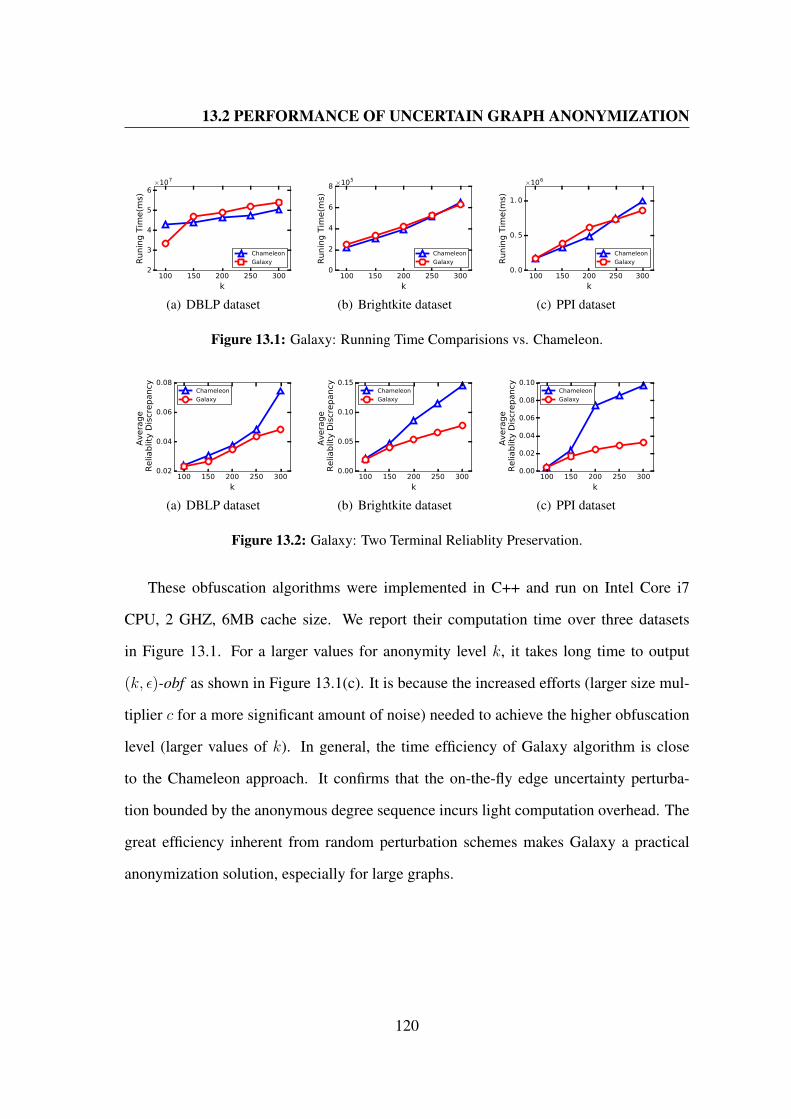
13.2 PERFORMANCE OF UNCERTAIN GRAPH ANONYMIZATION
100 150 200 250 300
k
2
3
4
5
6
Runin
g T
ime(m
s)
×107
Chameleon
Galaxy
(a) DBLP dataset
100 150 200 250 300
k
0
2
4
6
8
Runin
g T
ime(m
s)
×105
Chameleon
Galaxy
(b) Brightkite dataset
100 150 200 250 300
k
0. 0
0. 5
1. 0
Runin
g T
ime(m
s)
×106
Chameleon
Galaxy
(c) PPI dataset
Figure 13.1: Galaxy: Running Time Comparisions vs. Chameleon.
100 150 200 250 300
k
0.02
0.04
0.06
0.08
Avera
ge
Relia
blit
y D
iscr
epancy Chameleon
Galaxy
(a) DBLP dataset
100 150 200 250 300
k
0.00
0.05
0.10
0.15
Avera
ge
Relia
blit
y D
iscr
epancy Chameleon
Galaxy
(b) Brightkite dataset
100 150 200 250 300
k
0.00
0.02
0.04
0.06
0.08
0.10
Avera
ge
Relia
blit
y D
iscr
epancy Chameleon
Galaxy
(c) PPI dataset
Figure 13.2: Galaxy: Two Terminal Reliablity Preservation.
These obfuscation algorithms were implemented in C++ and run on Intel Core i7
CPU, 2 GHZ, 6MB cache size. We report their computation time over three datasets
in Figure 13.1. For a larger values for anonymity level k, it takes long time to output
(k, ε)-obf as shown in Figure 13.1(c). It is because the increased efforts (larger size mul-
tiplier c for a more significant amount of noise) needed to achieve the higher obfuscation
level (larger values of k). In general, the time efficiency of Galaxy algorithm is close
to the Chameleon approach. It confirms that the on-the-fly edge uncertainty perturba-
tion bounded by the anonymous degree sequence incurs light computation overhead. The
great efficiency inherent from random perturbation schemes makes Galaxy a practical
anonymization solution, especially for large graphs.
120

13.2 PERFORMANCE OF UNCERTAIN GRAPH ANONYMIZATION
100 150 200 250 300
k
0.0
0.1
0.2
0.3
0.4
0.5
Rela
tive E
rror
Degre
e
Chamelon
Galaxy
(a) DBLP dataset
100 150 200 250 300
k
0.0
0.5
1.0
1.5
2.0
Rela
tive E
rror
Degre
e
Chamelon
Galaxy
(b) Brightkite dataset
100 150 200 250 300
k
0
1
2
3
4
Rela
tive E
rror
Degre
e
Chamelon
Galaxy
(c) PPI dataset
Figure 13.3: Galaxy: The Change Ratio of Degree.
13.2.2 Utility Loss Evaluation
Reliability Preserving In particular, we report the average reliability discrepancy of
anonymized graphs in Figure 9.2. The smaller discrepancy, the better the reliability
preserving, the better graph structure preserving. It shows that when the k requirement
increases, the amount of distortion also increases. The proposed anonymous degree se-
quence bounded approach Galaxy has shown improved utility preservation in most cases
of different uncertain graph types and sizes. For instance, in PPI dataset (k = 300),
the reliability discrepancy introduced by Galaxy approach is well below 5%, while the
one of Chameleon is around 10%. This improvement is significant on the larger dataset,
e.g., DBLP dataset. The perturbation model dervived by anonymized degree sequence
alignment guides edge probability perturbation wisely.
Global Statistics Preserving For other statistics, we computed the average statistical
error, that is, the relative absolute difference between the estimation and the real value.
The smaller error, the better utility preserving.
Figure 13.4 and Figure 13.5 report the comparison of uncertain graph anonymization
approaches regarding their ability to preserve the average path distance and clustering
coefficient respectively. The other shortest-path based statistics share almost exact tren-
dency with the average path distanace. Therefore, we omit them.Conversely, for small
values of k, e.g., k = 100, errors introduced by Galaxy approaches are always smaller
121

13.2 PERFORMANCE OF UNCERTAIN GRAPH ANONYMIZATION
100 150 200 250 300
k
0.0
0.1
0.2
0.3
0.4
0.5
Rela
tive E
rror
Avera
ge D
ista
nce
Chamelon
Galaxy
(a) DBLP dataset
100 150 200 250 300
k
0.0
0.1
0.2
0.3
0.4
0.5
Rela
tive E
rror
Avera
ge D
ista
nce
Chamelon
Galaxy
(b) Brightkite dataset
100 150 200 250 300
k
0.0
0.1
0.2
0.3
0.4
0.5
Rela
tive E
rror
Avera
ge D
ista
nce
Chamelon
Galaxy
(c) PPI dataset
Figure 13.4: Galaxy: Average Path Distance Preservation.
100 150 200 250 300
k
0.00
0.01
0.02
0.03
0.04
0.05
Rela
tive E
rror
Clu
steri
ng C
oeff
icie
nt
Chamelon
Galaxy
(a) DBLP dataset
100 150 200 250 300
k
0.0
0.1
0.2
0.3
Rela
tive E
rror
Clu
steri
ng C
oeff
icie
nt
Chamelon
Galaxy
(b) Brightkite dataset
100 150 200 250 300
k
0.0
0.2
0.4
0.6
0.8
Rela
tive E
rror
Clu
steri
ng C
oeff
icie
nt
Chamelon
Galaxy
(c) PPI dataset
Figure 13.5: Galaxy: Clustering Coefficient Preservation.
than 1%. The larger values of k, the larger errors introduced. Generally, at the same
level of identity obfuscation our Galaxy method provides higher utility than the existing
chameleon method. Take SAPD error when k = 200 as example. As depicted in Fig-
ure 13.4, the change ratio of our Galaxy method is around 10% for DBLP, and PPI,
while that under Chameleon is 30% for DBLP and Brightkite. The other example is
Scc value. As depicted in Figure 13.5, our Galaxy method caused around 0.039 and 0.08
utility loss on average for Brightkite and PPI respectively. On contrary, Chameleon
cause 0.149 and 0.081 utility loss on average. All these observations verify that “anony-
mous degree sequence” bounded strategy does successfully avoid void edge uncertainty
perturbation, as our Galaxy method is most effective.
The behavior described for scalar statistics is also observed with vector statistics. For
example, Figure 13.6 shows the degree distribution in the original PPI and in obfuscated
versions. Here, six extreme cases are presented: For k = 100, 200, 300 and ε = 10−2
122
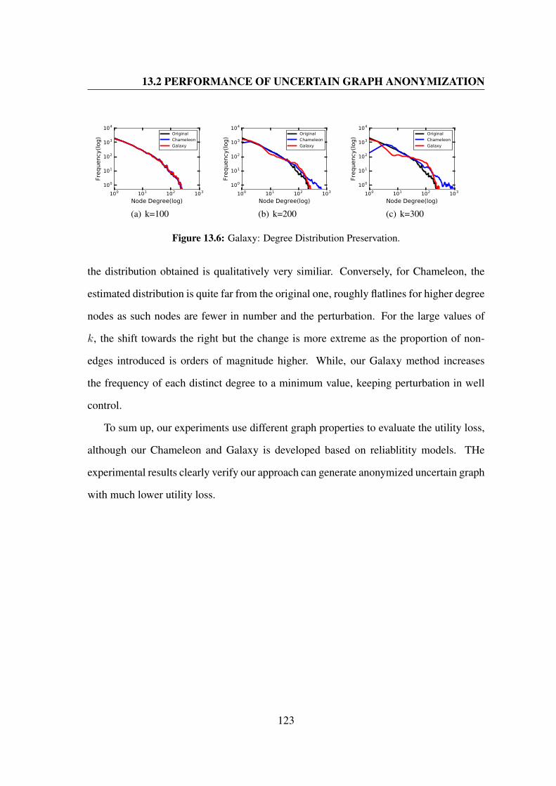
13.2 PERFORMANCE OF UNCERTAIN GRAPH ANONYMIZATION
100 101 102 103
Node Degree(log)
100
101
102
103
104
Frequency
(log)
Original
Chameleon
Galaxy
(a) k=100
100 101 102 103
Node Degree(log)
100
101
102
103
104
Frequency
(log)
Original
Chameleon
Galaxy
(b) k=200
100 101 102 103
Node Degree(log)
100
101
102
103
104
Frequency
(log)
Original
Chameleon
Galaxy
(c) k=300
Figure 13.6: Galaxy: Degree Distribution Preservation.
the distribution obtained is qualitatively very similiar. Conversely, for Chameleon, the
estimated distribution is quite far from the original one, roughly flatlines for higher degree
nodes as such nodes are fewer in number and the perturbation. For the large values of
k, the shift towards the right but the change is more extreme as the proportion of non-
edges introduced is orders of magnitude higher. While, our Galaxy method increases
the frequency of each distinct degree to a minimum value, keeping perturbation in well
control.
To sum up, our experiments use different graph properties to evaluate the utility loss,
although our Chameleon and Galaxy is developed based on reliablitity models. THe
experimental results clearly verify our approach can generate anonymized uncertain graph
with much lower utility loss.
123

Part IV
Conclusion and Future Work
124

14
Conclusion of This Dissertation
The goal of this dissertation is to fill the void in the literature of effectively anonymizing
uncertain graphs. Uncertain graphs serve as a powerful model to capture the complicated
relationship in a wide range of applications—business to business (B2B), social networks
and sensor networks. These uncertain graphs are of significance in the analytic and knowl-
edge extraction. However, such data are rarely released to the public for research due to
privacy and security concerns. Conventional approaches on graph anonymization mainly
focused on the determintitic graph. In this dissertation, we propose novel techniques and
systems to address newly identified privacy risks caused by the revealed edge uncertainty.
Within this scope, we focus on two research aspects, namely methods and systems for
resisting different types of de-anonymization where the adversary has the prior knowledge
of the victim node such as degree static or probabilistic degree distribution.
First, we focus on the problem of identity obfuscation over uncertain graphs. We
model the adversary’s prior knowledge as the degree (expectation) of a target node. To
mitigate such privack attack, we propose an uncertainty semantic based perturbation
scheme Chameleon that ensure the lowebound of anonymity provided of the majority of
nodes. Chameleon offers 3 key innovation (1) We introduce a new reliablity-based utility
125
metric for capturing the structural distortion introduced by anonymization scheme. (2)
We introduce a theoretically-founded criterion, called reliability relevance, that encodes
the sensitivity of the graph edges and vertices to the possible injected perturbation. The
criterion will guide the edges’ selection during the anonymization process. (3) We pro-
pose uncertainty-aware heuristics for efficient edge selection and noise injection over the
input uncertain graph to achieve anonymization at a slight cost of data utility. Our com-
prehensive experimental study confirms its efficiency in utility preservation compared to
the conventional methods that do not directly consider edge uncertainties.
Second, we address the problem of resisting probabilistic degree-based de-anonymization
on anonymized uncertain graphs. We model the adversary’s prior knowledge as the de-
gree (distribution) of a target node. To address this challenge, we propose an uncertainty
semantic based perturbation scheme Galaxy. Our Galaxy system offers three key inno-
vation: (1) We adopt the defintion of k-obfuscation by introducing fuzzy equvialance
relation in the context of uncertain graph. (2)We propose a two-phase framework that
first construct a probabilistic degree sequence that over k-obfuscates target nodes and use
derived alginment varitation as weighting factor for guiding perturbation for construct-
ing anonymous uncertain graph. (3)We propose a light-weight anonymity quantification
operation which provides exact evaluation w.r.t k-obfuscation for speeding up the graph
construction process.
126

15
Future Work
15.1 Defeating More Involved De-anonymization Attacks
As ever discussed, the adversary can use a handful of local structural signatures about the
nodes/community of an uncertain graph to de-anonymize the individual in the anonymized
graph. Examples of local structural features are node’s degree, node’s clustering coeffi-
cient, edge density of the node’s neighbors, etc. The utilization of such local structural
features has been investigated comprehensively in the context of deterministic graphs
since they are important auxiliary information used in the de-anonymization attack. To
date, they have not yet been considered in the context of uncertain graphs. We ever
present a new class of de-anonymization attacks against uncertain graphs which incor-
porate with edge uncertainty in the published uncertain graphs. While more involved
de-anonymization attack models remain unexplored.
In this dissertation, we first identified the potential privacy attack over uncertain graphs
where edge uncertainty can be leveraged in de-anonymization. We focus on prevent-
ing node re-identification attacks triggered by the highly revealing information, node’s
degree—one of the most common structural information used in the de-anonymization.
127

15.1 DEFEATING MORE INVOLVED DE-ANONYMIZATION ATTACKS
Our proposed solution is tailored towards uncertain graph, while is designed to defeat
only a narrow set of attacks.
In practice, it is not realistic to assume that an adversary has only a narrow set of
the priori knowledge in the original uncertain graph. Therefore, the uncertain graph
anonymization framework should consider different kinds of privacy attacks such as the
count of small subgraphs (triangles, stars) ones. Moreover, it is not realistic to assume that
an adversary would launch only one type of attacks for uncertain graphs, i.e., an adver-
sary has only one type of structural information about the target node in the anonymized
graph. As our future work, we plan to consider more powerful attacks i.e. the combination
of other kinds of structural information such as the number of triangles, node between-
ness, the embedded subgraph information. Therefore, an uncertain graph anonymiza-
tion framework should work under the assumption that there will be simultaneous mul-
tiple attacks and techniques to be resilient to all of them. We plan to design a genetic
uncertainty-semantic-aware framework to shift existing deterministic graph anonymiza-
tion techniques to the case of uncertain graphs for incremental contributions.
The intuition of how to adopt existing graph anonymization techniques is as follows.
Namely, we utilize the probabilistic structural signature to partition sensitive entities
(nodes, links, subgraphs) in the given uncertain graphs, called anonymized fragments.
We first probe a solution of anonymized fragments based upon the user-defined privacy
condition. In other words, an uncertain graph that realized such anonymized representa-
tion can provide the desirable anonymity. Then, semi-randomized uncertainty-semantic
based perturbation algorithms can be used for probing the anonymous graph instance.
Heuristic stems from the discrepancy could be weighting factor to guide anonymization
process.
128

15.2 BIG GRAPH ANONYMIZATION
15.2 Big Graph Anonymization
Web2.0 fueled interest in social networks. Other large graphs—for example, graphs in-
duced by transportation routes, paths of disease outbreak, or citation relationships among
published scientific work–have attracted research interests. Publishing such graph data
would allow a wide variety of ad hoc analyses over real large graph datasets and fueled
valid use of the data. Meanwhile, it also raises huge privacy concerns. Such graph data
contain sensitive information about the graph entities as well as their connections, whose
disclosure may violate privacy regulations. The privacy violation may be caused by the
de-anonymization attack such as identifying node via its subgraph signatures, or via corre-
lation with overlapping graphs. Although many advanced graph anonymization methods
have been proposed to mitigate such risks, the majority of existing graph (deterministic
& uncertain ) anonymization algorithms are designed to defeat privacy attacks for graphs
in a small or medium size. The majority of existing graph anonymization techniques are
either difficult to scale up to multi-GB to TBs of graph data or efficiency intractable. In
summary, the increasing sizes of graph data sets present a significant challenge to graph
anonymization algorithm.
Since the amount of data to be anonymized has grossly outpaced advances in the mem-
ory available on commodity hardware, we plan to leverage parallel graph anonymization
algorithm to defeat sensitive information disclosure. The main intuition of parallelizing
existing graph anonymization algorithm stemmed from the programming model of paral-
lel and distributed graph processing systems. The growing scale and importance of graph
data have driven the development of numerous specialized graph processing systems in-
cluding Pregel [1], PowerGraph [2], GraphX[15] and many others [42, 55]. By exposing
specialized abstractions backed by graph-specific optimization, these systems can natu-
rally express and efficiently execute iterative graph algorithm on web-scale graphs. For
129

15.3 LEARNING TO ANONYMIZE UNCERTAIN GRAPHS
Figure 15.1: Parallel Graph Anonymization Process.
example, for the sake of maximizing parallelism and scalability, Pregel [1] adopts a non-
traditional programming model where a graph algorithm is implemented as single com-
putation function written in a vertex-centric, message-passing and bulk-synchronous way.
Interestingly, many graph anonymization methods can be naturally expressed as vertex-
centric perturbation such as random perturbation schemes [32, 33, 34].Typical graph
anonymization algorithms are composed of multiple computation kernels connected by
non-trivial control flows such as privacy risk assessment, utility cost evaluation, perturba-
tion generation. Together, we believe it is a promising direction of solving the big graph
anonymization problem.
15.3 Learning to Anonymize Uncertain Graphs
Data privacy is a major problem that has to be considered before releasing datasets to the
public or even a partner company that would compute statistics or make an in-depth anal-
ysis of the dataset. In the context of graphs (deterministic & uncertain), many different
anonymization techniques have been proposed. However, these methods including our
130
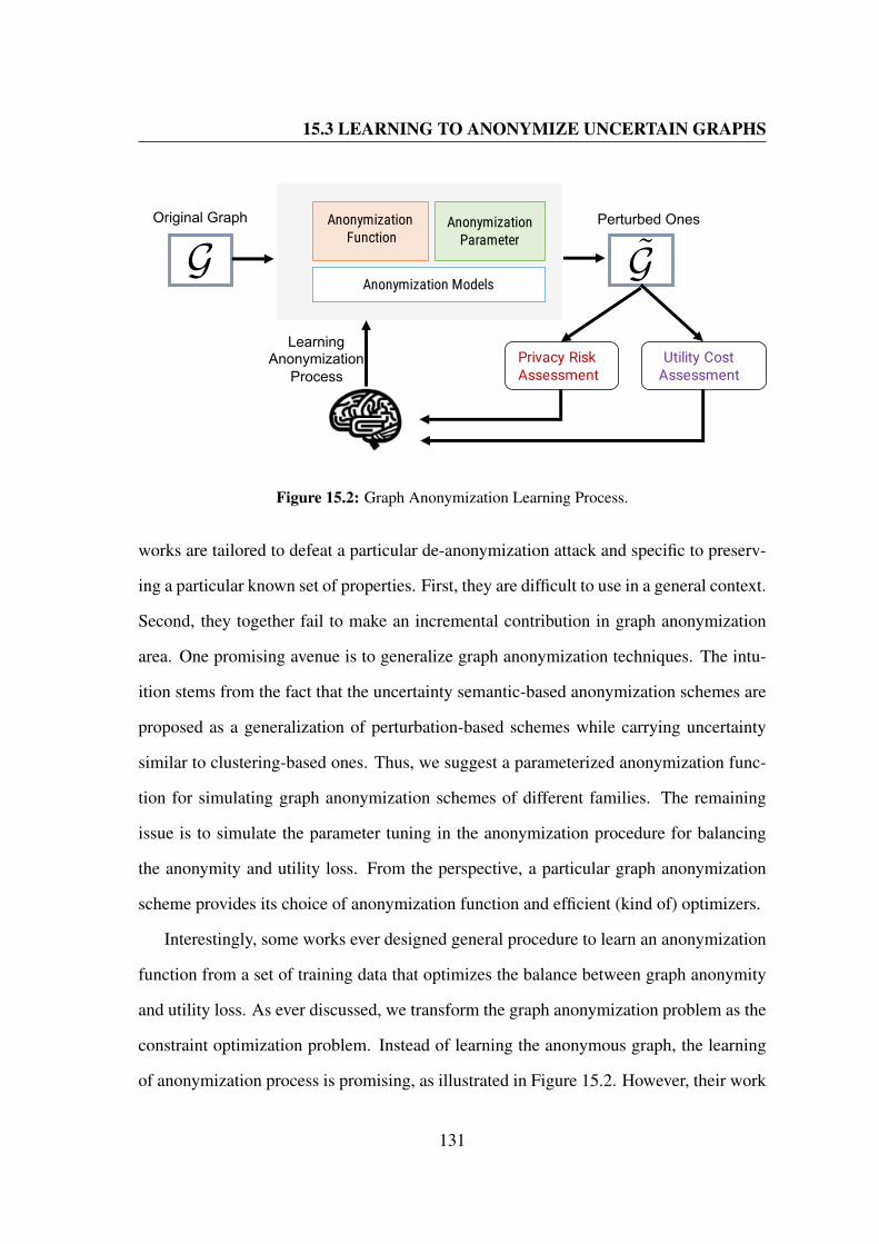
15.3 LEARNING TO ANONYMIZE UNCERTAIN GRAPHS
AnonymizationFunction
AnonymizationParameter
Anonymization ModelsG G
Privacy RiskAssessment
Utility CostAssessment
LearningAnonymization
Process
Original Graph Perturbed Ones
Figure 15.2: Graph Anonymization Learning Process.
works are tailored to defeat a particular de-anonymization attack and specific to preserv-
ing a particular known set of properties. First, they are difficult to use in a general context.
Second, they together fail to make an incremental contribution in graph anonymization
area. One promising avenue is to generalize graph anonymization techniques. The intu-
ition stems from the fact that the uncertainty semantic-based anonymization schemes are
proposed as a generalization of perturbation-based schemes while carrying uncertainty
similar to clustering-based ones. Thus, we suggest a parameterized anonymization func-
tion for simulating graph anonymization schemes of different families. The remaining
issue is to simulate the parameter tuning in the anonymization procedure for balancing
the anonymity and utility loss. From the perspective, a particular graph anonymization
scheme provides its choice of anonymization function and efficient (kind of) optimizers.
Interestingly, some works ever designed general procedure to learn an anonymization
function from a set of training data that optimizes the balance between graph anonymity
and utility loss. As ever discussed, we transform the graph anonymization problem as the
constraint optimization problem. Instead of learning the anonymous graph, the learning
of anonymization process is promising, as illustrated in Figure 15.2. However, their work
131

15.3 LEARNING TO ANONYMIZE UNCERTAIN GRAPHS
limits on simulating perturbation-based schemes. While the random perturbation-based
anonymization schemes usually suffer from high bound of utility cost. Experiments [] that
it is hard to provide anonymity while preserving utility whereas some perturbation-based
schemes destroy utility without providing much anonymity.
Moreover, their general learning process ignores the property of anonymization func-
tion. Therefore, it accompanies with inefficient convergence rate. In particular, it is not
guaranteed to converge to a local optimal anonymization model for large graph dataset.
Besides, this method relies on using the large population of graphs with similar proper-
ties for the training step. It is not realistic to assume the existence and availability of
homogeneous graph datasets. We plan to design a genetic machine learning framework
for generalizing existing graph anonymization methods with more flexibility. The intu-
ition of how to generalize graph anonymization method is as follows. Instead of defining
a specific anonymization function, the user defines a set of multi-classed parameterized
function procedures, they together controlling the behavior of the anonymization process.
We consider the mixture of the different family of graph anonymizations over anonymiza-
tion stages. The machine learning framework will be able to provide the best model that
corresponds to the complex anonymization procedure that obtains the best balance be-
tween anonymization quality and utility loss in the user-defined anonymous graph space.
In summary, it would be interesting and promising to explore these three directions.
We hope the experimental evaluation can confirm the superiority of the approaches/models
above. Eventually, future work in this direction will significantly enhance the applicabil-
ity of our next generation graph anonymization system to a wider spectrum.
132

References
[1] Grzegorz Malewicz, Matthew H. Austern, Aart J.C Bik, James C. Dehnert, Ilan
Horn, Naty Leiser, and Grzegorz Czajkowski. Pregel: A system for large-scale
graph processing. In SIGMOD, pages 135–146, 2010. 1, 2, 7, 15, 17, 56, 129, 130
[2] Joseph E. Gonzalez, Yucheng Low, Haijie Gu, Danny Bickson, and Carlos Guestrin.
Powergraph: Distributed graph-parallel computation on natural graphs. OSDI, pages
17–30, 2012. 1, 2, 15, 17, 129
[3] JP Eckmann and E Moses. Curvature of co-links uncovers hidden thematic layers
in the world wide web. Academy of Sciences, 2002. 1, 2
[4] S Khuller and B Saha. On finding dense subgraphs. Automata, 2009. 1, 2
[5] L Becchetti, P Boldi, C Castillo, and A Gionis. Efficient semi-streaming algorithms
for local triangle counting in massive graphs. KDD, pages 16–24, 2008. 1, 2, 25
[6] R Milo, S Shen-Orr, S Itzkovitz, N Kashtan, and D Chklovskii. Network motifs:
simple building blocks of complex networks. Academy of Sciences, 2002. 2
[7] JW Berry, B Hendrickson, RA LaViolette, and CA Phillips. Tolerating the com-
munity detection resolution limit with edge weighting. Physical Review E, 2011.
2
133

REFERENCES
[8] LS Buriol, G Frahling, and S Leonardi. Counting triangles in data streams. PODS,
pages 253–262, 2006. 2
[9] Xiaocheng Hu, Yufei Tao, and Chin-Wan Chung. I/o-efficient algorithms on triangle
listing and counting. ACM Trans. Database Syst., 39(4), 2014. 2, 6, 54, 55
[10] J Kim, WS Han, S Lee, K Park, and H Yu. Opt: a new framework for overlapped
and parallel triangulation in large-scale graphs. SIGMOD, pages 637–648, 2014. 2,
6, 54, 55
[11] Aapo Kyrola, Guy Blelloch, and Carlos Guestrin. Graphchi: Large-scale graph
computation on just a pc. OSDI, pages 31–46, 2012. 2, 6, 54
[12] Shaikh Arifuzzaman, Maleq Khan, and Madhav Marathe. Patric: A parallel algo-
rithm for counting triangles in massive networks. CIKM, pages 529–538, 2013. 2,
7, 24, 25, 27, 55
[13] Siddharth Suri and Sergei Vassilvitskii. Counting triangles and the curse of the last
reducer. KDD, pages 607–614, 2011. 2, 6, 24, 25, 26, 27, 28, 46, 55
[14] Wook-Shin Han, Sangyeon Lee, Kyungyeol Park, Jeong-Hoon Lee, Min-Soo Kim,
Jinha Kim, and Hwanjo Yu. Turbograph: a fast parallel graph engine handling
billion-scale graphs in a single pc. KDD, pages 77–85, 2013. 2
[15] JE Gonzalez, RS Xin, A Dave, and D Crankshaw. Graphx: Graph processing in
a distributed dataflow framework. GRADES,SIGMOD workshop, pages 599–613,
2014. 2, 15, 17, 129
[16] Mingfeng Lin, Mei Lin, and Robert J. Kauffman. From clickstreams to search-
streams: Search network graph evidence from a b2b e-market. ICEC, 2012. 3,
4
134

REFERENCES
[17] E Adar and C Re. Managing uncertainty in social networks. IEEE Data Eng. Bull.,
2007. 3, 58
[18] D Kempe, J Kleinberg, and E Tardos. Maximizing the spread of influence through
a social network. 2003. 3, 58, 60, 101
[19] Liang Zhang, Shigang Chen, Ying Jian, Yuguang Fang, and Zhen Mo. Maximizing
lifetime vector in wireless sensor networks. IEEE/ACM Trans. Netw., 2013. 3
[20] K Bollacker, C Evans, P Paritosh, and T Sturge. Freebase: a collaboratively created
graph database for structuring human knowledge. SIMMOD, 2008. 3
[21] NJ Krogan, G Cagney, H Yu, G Zhong, and X Guo. Global landscape of protein
complexes in the yeast saccharomyces cerevisiae. Nature, 2006. 3
[22] Eunjoon Cho, Seth A Myers, and Jure Leskovec. Friendship and mobility: user
movement in location-based social networks. kdd, 2011. 3, 84
[23] B Zhao, J Wang, M Li, FX Wu, and Y Pan. Detecting protein complexes based
on uncertain graph model. IEEE/ACM Transactions on Computational Biology and
Bioinformatics., 2014. 3, 18, 58, 60, 101
[24] D Liben Nowell and J Kleinberg. The link prediction problem for social networks.
The American Society for Information Science and Technology, 2007. 4
[25] Alan S. Abrahams, Eloise Coupey, Eva X. Zhong, Reza Barkhi, and Pete S. Man-
asantivongs. Audience targeting by b-to-b advertisement classification: A neural
network approach. Expert Systems with Applications, 40(8):2777 – 2791, 2013. 4
[26] T. Alsina, D.T. Wilson, S.A. Joshi, and S. Sundaresan. Targeting customer segments,
December 3 2015. US Patent App. 14/289,118. 4
135

REFERENCES
[27] Kun Liu and Evimaria Terzi. Towards identity anonymization on graphs. SIGMOD,
2008. 5, 8, 11, 13, 59, 66, 92, 93, 95, 105
[28] Paolo Boldi, Francesco Bonchi, Aristides Gionis, and Tamir Tassa. Injecting uncer-
tainty in graphs for identity obfuscation. SIGMOD, 2012. 5, 8, 12, 13, 59, 62, 66,
67, 68, 76, 83, 85, 86, 93, 94, 100
[29] P Mittal, C Papamanthou, and D Song. Preserving link privacy in social network
based systems. NDSS, 2013. 5, 62, 76, 93, 94
[30] HH Nguyen, A Imine, and M Rusinowitch. Anonymizing social graphs via uncer-
tainty semantics. CCS, 2015. 5, 12, 62, 76, 85, 93, 94
[31] L Liu, J Wang, J Liu, and J Zhang. Privacy preservation in social networks with
sensitive edge weights. SDM, pages 954–965, 2009. 5, 66, 67, 92, 93, 94, 95
[32] Xiaowei Ying and Xintao Wu. Randomizing social networks: a spectrum preserving
approach. pages 739–750, 2008. 5, 10, 13, 66, 67, 92, 93, 130
[33] Mohd Ninggal and Jemal H Abawajy. Utility-aware social network graph
anonymization. J Netw Comput Appl, 2015. 5, 13, 66, 67, 92, 93, 130
[34] Francesco Bonchi, Aristides Gionis, and Tamir Tassa. Identity obfuscation in graphs
through the information theoretic lens. ICDE, 2014. 5, 59, 92, 93, 100, 130
[35] N. Alon, R. Yuster, and U. Zwick. Finding and counting given length cycles. Algo-
rithmica, 1997. 5, 54
[36] V Batagelj and A Mrvar. A subquadratic triad census algorithm for large sparse
networks with small maximum degree. Social networks, 2001. 5, 54
[37] T Schank. Algorithmic aspects of triangle-based network analysis. Phd in computer
science, 2007. 5, 25, 36, 54
136
REFERENCES
[38] A Itai and M Rodeh. Finding a minimum circuit in a graph. SIAM, 1978. 5, 54
[39] N Chiba and T Nishizeki. Arboricity and subgraph listing algorithms. SIAM Journal
on Computing, 1985. 5, 54
[40] Ha-Myung Park, Francesco Silvestri, U Kang, and Rasmus Pagh. MapReduce tri-
angle enumeration with guarantees. CIKM, pages 1739–1748, 2014. 6, 24, 26,
55
[41] Carlos H. C. Teixeira, Alexandre J. Fonseca, Marco Serafini, Georgos Siganos, Mo-
hammed J. Zaki, and Ashraf Aboulnaga. Arabesque: a system for distributed graph
mining. SOSP, pages 425–440, 2015. 6, 55
[42] Yingxia Shao, Bin Cui, Lei Chen, Lin Ma, Junjie Yao, and Ning Xu. Parallel sub-
graph listing in a large-scale graph. SIGMOD, pages 625–636, 2014. 7, 56, 129
[43] Wentao Wu, Yanghua Xiao, Wei Wang, Zhenying He, and Zhihui Wang. k-
symmetry model for identity anonymization in social networks. EDBT, 2010. 8,
66, 67, 92, 93
[44] Bin Zhou and Jian Pei. Preserving privacy in social networks against neighborhood
attacks. ICDE, 2008. 8, 66, 92, 93
[45] L Backstrom, C Dwork, and J Kleinberg. Wherefore art thou r3579x?: anonymized
social networks, hidden patterns, and structural steganography. WWW, 7 2007. 8
[46] Arvind Narayanan and Vitaly Shmatikov. De-anonymizing social networks. SP,
pages 173–187, 2009. 8
[47] Shixi Chen and Shuigeng Zhou. Recursive mechanism: Towards node differential
privacy and unrestricted joins. SIGMOD, pages 653–664, 2013. 9
137
REFERENCES
[48] Michael Hay, Gerome Miklau, David Jensen, Philipp Weis, and Siddharth Srivas-
tava. Anonymizing social networks. 2007. 10, 92, 93
[49] Smriti Bhagat, Graham Cormode, Balachander Krishnamurthy, and Divesh Srivas-
tava. Class-based graph anonymization for social network data. Proc Vldb Endow,
2009. 10, 92, 93
[50] Xiaowei Ying, Kai Pan, Xintao Wu, and Ling Guo. Comparisons of randomization
and k-degree anonymization schemes for privacy preserving social network publish-
ing. SNA-KDD, 2009. 10, 11, 66
[51] Sepp Hartung and Nimrod Talmon. The complexity of degree anonymization by
graph contractions. TAMC, 2015. 11, 15
[52] Ewni: Efficient anonymization of vulnerable individuals in social networks.
PAKDD, 7302:359370, 2012. 11
[53] Xuesong Lu, Yi Song, and Stphane Bressan. Database and expert systems applica-
tions. DEXA, 7446:281295, 2012. 11
[54] Yazhe Wang, Long Xie, Baihua Zheng, and Ken C. K. Lee. Utility-oriented k-
anonymization on social networks. DASFAA, 2011. 13, 66, 67, 92, 93
[55] S Salihoglu and J Widom. Gps: A graph processing system. SSDBM, 2013. 16, 31,
129
[56] Nguyen Bao and Toyotaro Suzumura. Towards highly scalable pregel-based graph
processing platform with x10. WWW, 2013. 16, 31
[57] S Asthana, OD King, FD Gibbons, and FP Roth. Predicting protein complex mem-
bership using probabilistic network reliability. Genome research, 2004. 18
138

REFERENCES
[58] J Ghosh, HQ Ngo, and S Yoon. On a routing problem within probabilistic graphs
and its application to intermittently connected networks. 2007. 18, 60, 101
[59] Jeffrey Dean and Sanjay Ghemawat. Mapreduce: Simplified data processing on
large clusters. Commun. ACM, 2008. 26
[60] Tom White. Hadoop: The definitive guide. 2010. 26
[61] Anish Das Sarma, Foto N. Afrati, Semih Salihoglu, and Jeffrey D. Ullman. Upper
and lower bounds on the cost of a map-reduce computation. PVLDB, 2013. 29
[62] J Lin. The curse of zipf and limits to parallelization: A look at the stragglers problem
in mapreduce. LSDR-IR workshop, 2009. 29
[63] Gary W. Oehlert. A note on the delta method. The American Statistician, 1992. 30
[64] G Keramidas and P Petoumenos. Cache replacement based on reuse-distance pre-
diction. ICCD, 2007. 41
[65] P Petoumenos and G Keramidas. Instruction-based reuse-distance prediction for
effective cache management. MSP, pages 60–68, 2009. 41
[66] M Potamias, F Bonchi, A Gionis, and G Kollios. K-nearest neighbors in uncertain
graphs. VLDB, 2010. 58, 60, 86, 95, 101
[67] M Hua and J Pei. Probabilistic path queries in road networks: traffic uncertainty
aware path selection. EDBT, 2010. 58
[68] R Jin, L Liu, B Ding, and H Wang. Distance-constraint reachability computation in
uncertain graphs. VLDB, 2011. 58, 83, 86
139
REFERENCES
[69] Michael Hay, Gerome Miklau, David Jensen, Don Towsley, and Chao Li. Resist-
ing structural re-identification in anonymized social networks. The VLDB Journal,
2010. 59, 92, 93
[70] Colbourn and Colbourn. The combinatorics of network reliability. 1987. 60
[71] Parchas, Gullo, Papadias, and Bonchi. The pursuit of a good possible world: ex-
tracting representative instances of uncertain graphs. SIGMOD, 2014. 62, 63, 86
[72] Jordi Casas-Roma. Privacy-preserving on graphs using randomization and edge-
relevance. Modeling Decisions for Artificial Intelligence, 2015. 66, 67, 92, 93
[73] Brian Thompson and Danfeng Yao. The union-split algorithm and cluster-based
anonymization of social networks. 2009. 66, 92, 93
[74] Sudipto Das, Omer Egecioglu, and Amr Abbadi. Anonymizing weighted social
network graphs. ICDE, pages 904–907, 2010. 66, 67, 92, 93, 94, 95
[75] M. O. Ball. Computational complexity of network reliability analysis: An overview.
IEEE Transactions on Reliability, 1986. 71
[76] M. Fredman and M. Saks. The cell probe complexity of dynamic data structures.
STOC, 1989. 72
[77] P Boldi, M Rosa, and S Vigna. HyperANF: approximating the neighbourhood func-
tion of very large graphs on a budget. CoRR, 2011. 86
[78] G Cormode, D Srivastava, T Yu, and Q Zhang. Anonymizing bipartite graph data
using safe groupings. VLDB, 2008. 92, 93
[79] Shyue-Liang Wang, Yu-Chuan Tsai, Hung-Yu Kao, I-Hsien Ting, and Tzung-Pei
Hong. Shortest paths anonymization on weighted graphs. nternational Journal of
140

REFERENCES
Software Engineering and Knowledge Engineering, 23(01):65–79, 2013. 92, 93, 94,
95
[80] ME Skarkala, M Maragoudakis, S Gritzalis, L Mitrou, H Toivonen, and P Moen.
Privacy preservation by k-Anonymization of weighted social networks. ASONAM,
2012. 92, 93, 94, 95
141