towards digital image anti-forensics via image restoration · (iii) jpeg anti-forensics using jpeg...
TRANSCRIPT
Towards digital image anti-forensics via image
restoration
Wei Fan
To cite this version:
Wei Fan. Towards digital image anti-forensics via image restoration. Signal and Image process-ing. Universite Grenoble Alpes, 2015. English. <NNT : 2015GREAT035>. <tel-01216243>
HAL Id: tel-01216243
https://tel.archives-ouvertes.fr/tel-01216243
Submitted on 15 Oct 2015
HAL is a multi-disciplinary open accessarchive for the deposit and dissemination of sci-entific research documents, whether they are pub-lished or not. The documents may come fromteaching and research institutions in France orabroad, or from public or private research centers.
L’archive ouverte pluridisciplinaire HAL, estdestinee au depot et a la diffusion de documentsscientifiques de niveau recherche, publies ou non,emanant des etablissements d’enseignement et derecherche francais ou etrangers, des laboratoirespublics ou prives.
THÈSEpour obtenir le grade de
DOCTEUR DE L’UNIVERSITÉ DE GRENOBLE ALPES
préparée dans le cadre d’une cotutelle entrel’Université Grenoble Alpes et Beihang University
Spécialité : signal, image, parole, télécommunications (SIPT)
Arrêté ministériel : le 6 janvier 2005 - 7 août 2006
Présentée par
Wei FAN
Thèse dirigée par Jean-Marc BROSSIER et Zhang XIONGet encadrée par François CAYRE et Kai WANG
préparée au sein du laboratoire Grenoble, images, parole,signal, automatique (GIPSA-lab) et School of ComputerScience and Engineering
dans l’école doctorale d’électronique, électrotechnique,automatique et traitement du signal (EEATS) et BeihangUniversity
Vers l’anti-criminalistiqueen images numériquesvia la restauration d’imagesThèse soutenue publiquement le 30/04/2015,
devant le jury composé de:
Jean-Marc CHASSERYDirecteur de Recherche CNRS, GIPSA-lab, Examinateur, Président
Jean-Luc DUGELAYProfesseur, EURECOM, Sophia Antipolis, Rapporteur
Stefano TUBAROProfesseur, Politecnico di Milano, Rapporteur
Teddy FURONChargé de Recherche INRIA, INRIA Rennes, Examinateur
Jiwu HUANGProfesseur, Shenzhen University, Examinateur
Zhang XIONGProfesseur, Beihang University, Co-directeur
François CAYREMaître de Conférences, Grenoble INP, GIPSA-lab, Co-encadrant
Kai WANGChargé de Recherche CNRS, GIPSA-lab, Co-encadrant


UNIVERSITY OF GRENOBLE ALPES
Doctoral school EEATS(Électronique, Électrotechnique, Automatique et Traitement du Signal)
T H E S I Sfor obtaining the title of
Doctor of Science
of the University of Grenoble Alpes
Speciality: SIPT(Signal, Image, Parole, Télécommunications)
Presented by
Wei FAN
Towards Digital Image Anti-Forensics
via Image Restoration
Thesis supervised by Jean-Marc BROSSIER and Zhang XIONGand co-supervised by François CAYRE and Kai WANG
prepared atGrenoble - Images, Parole, Signal, Automatique Laboratory (GIPSA-lab)
and School of Computer Science and Engineering, Beihang University
presented on 30/04/2015
Jury:
President: Jean-Marc CHASSERY - CNRS, GIPSA-labReviewers: Jean-Luc DUGELAY - EURECOM, Sophia Antipolis
Stefano TUBARO - Politecnico di MilanoExaminers: Teddy FURON - INRIA Rennes
Jiwu HUANG - Shenzhen UniversitySupervisor: Zhang XIONG - Beihang UniversityCo-Supervisors: François CAYRE - Grenoble INP, GIPSA-lab
Kai WANG - CNRS, GIPSA-lab


Acknowledgements
First and foremost, I would like to express my deepest gratitude to my four thesis supervi-sors: Prof. Jean-Marc Brossier, Dr. François Cayre, and Dr. Kai Wang in GIPSA-lab, andProf. Zhang Xiong in Beihang University. I am grateful to Prof. Brossier and Prof. Xiong,for offering me the wonderful opportunity to conduct a co-supervised Ph.D. thesis betweenGIPSA-lab/Grenoble INP and Beihang University. Not only did Dr. Cayre give me countlessinsightful suggestions on the research work, but he also consistently encouraged me when Ifaced difficulties. He created a motivating, pleasant and relaxing working environment, whereI could work effectively and at my pace. I owe my eternal thanks to Dr. Wang for his closeguidance as well as constant support, which pushed me to achieve what I never thought possi-ble. He is always patient in answering my questions, always efficient in correcting my mistakes,and always inspiring in our discussions, which are reflected throughout this thesis. Besides, Ialso would like to sincerely thank Prof. Gang Feng in GIPSA-lab and Prof. Shixiang Qian inBeihang University, who made this thesis opportunity accessible to me.
I would like to express my sincere gratitude to Prof. Jean-Luc Dugelay, and Prof. StefanoTubaro, for taking their precious time to review my thesis manuscript. I also would like togratefully thank Prof. Jean-Marc Chassery, Dr. Teddy Furon, and Prof. Jiwu Huang, forbeing examiners of my Ph.D. defense committee.
I am grateful to Dr. Xiyan He, who not only is a very good friend in the personal lifebut also provided me with insightful discussions on the total variation and the support vectormachine. I would like to thank Dr. Rodrigo Cabral Farias for answering my many mathe-matical questions and for referring me to many interesting materials. I am grateful to Dr.Zhenyong Chen and Ming Chen for their valuable suggestions and help when I started to workon multimedia security. I also want to thank Dr. Chuantao Yin and Hui Chen for their kindhelp and support for my coming to GIPSA-lab for study.
I want to thank my colleagues in the same office, Fatima, Jérémie, Fakhri, and Quentinin GIPSA-lab, and Shuo, Xiaolan, Jiahui, and Jianyuan in Beihang University, for creatingsuch a crazy, funny, and friendly office atmosphere. It was the best I could expect, especiallywhen there was a lot of stress from work. My thanks also go to Aude, Cyrille, Diyin, Gailene,Guanghan, Jonathan, Junshi, Longyu, Matthieu, Robin, Sheng, Vincent, Yang, Ying, andZhongyang for making my stay in France much easier. They have helped me during my dailylife in various forms, supporting me through hard times, integrating me into many interestingoutings and activities, introducing me to French culture, kindly helping me on my French, etc.
I am indebted to my dearest family, for their endless love and unconditional support. Nomatter how far away I am from home, it is the source of my strength knowing that they arealways there for me.
The work presented in this thesis is supported in part by the China Scholarship Councilunder Grant 2011602067, in part by the French ANR Estampille under Grant ANR-10-CORD-
v

vi
019, in part by the French Eiffel Scholarship under Grant 812587B, and in part by the FrenchRhône-Alpes region through the CMIRA Scholarship program. I would like to express mygratitude to them for the financial support, without which this thesis would not exist.

Abstract
Image forensics enjoys its increasing popularity as a powerful image authentication tool, work-ing in a blind passive way without the aid of any a priori embedded information comparedto fragile image watermarking. On its opponent side, image anti-forensics attacks forensicalgorithms for the future development of more trustworthy forensics. When image codingor processing is involved, we notice that image anti-forensics to some extent shares a similargoal with image restoration. Both of them aim to recover the information lost during theimage degradation, yet image anti-forensics has one additional indispensable forensic unde-tectability requirement. In this thesis, we form a new research line for image anti-forensics,by leveraging on advanced concepts/methods from image restoration meanwhile with inte-grations of anti-forensic strategies/terms. Under this context, this thesis contributes on thefollowing four aspects for JPEG compression and median filtering anti-forensics: (i) JPEGanti-forensics using Total Variation based deblocking, (ii) improved Total Variation basedJPEG anti-forensics with assignment problem based perceptual DCT histogram smoothing,(iii) JPEG anti-forensics using JPEG image quality enhancement based on a sophisticated im-age prior model and non-parametric DCT histogram smoothing based on calibration, and (iv)median filtered image quality enhancement and anti-forensics via variational deconvolution.Experimental results demonstrate the effectiveness of the proposed anti-forensic methods witha better forensic undetectability against existing forensic detectors as well as a higher visualquality of the processed image, by comparisons with the state-of-the-art methods.
Keywords: Image anti-forensics, image restoration, JPEG compression, median filtering
vii


Contents
Acknowledgements v
Abstract vii
Contents ix
List of Figures xv
List of Tables xix
Notations xxi
Acronyms xxv
1 Introduction 1
1.1 Can You Believe Your Eyes? . . . . . . . . . . . . . . . . . . . . . . . . . . . . . 1
1.2 Image Anti-Forensics . . . . . . . . . . . . . . . . . . . . . . . . . . . . . . . . . 3
1.3 Objectives and Contributions . . . . . . . . . . . . . . . . . . . . . . . . . . . . 4
1.3.1 JPEG Compression and Median Filtering . . . . . . . . . . . . . . . . . 4
1.3.2 Image Anti-Forensics and Image Restoration . . . . . . . . . . . . . . . . 6
1.3.3 Methodology . . . . . . . . . . . . . . . . . . . . . . . . . . . . . . . . . 6
1.4 Outline . . . . . . . . . . . . . . . . . . . . . . . . . . . . . . . . . . . . . . . . 7
2 Preliminaries 9
2.1 Classification of Image (Anti-)Forensics . . . . . . . . . . . . . . . . . . . . . . . 10
2.1.1 Farid’s Classification of Image Forensics . . . . . . . . . . . . . . . . . . 10
2.1.2 Redi et al.’s Classification of Image Forensics . . . . . . . . . . . . . . . 10
2.1.3 Piva’s Classification of Image Forensics . . . . . . . . . . . . . . . . . . . 11
2.1.4 Stamm et al.’s Classification of Image Forensics . . . . . . . . . . . . . . 12
2.1.5 Böhme and Kirchner’s Classification of Image Anti-Forensics . . . . . . 13
2.1.6 Classification of Proposed Anti-Forensic Methods . . . . . . . . . . . . . 14
2.2 Evaluation Metrics . . . . . . . . . . . . . . . . . . . . . . . . . . . . . . . . . . 14
2.2.1 Forensic (Un)detectability . . . . . . . . . . . . . . . . . . . . . . . . . . 15
2.2.2 Image Quality . . . . . . . . . . . . . . . . . . . . . . . . . . . . . . . . . 21
ix

x Contents
2.2.3 Histogram Recovery . . . . . . . . . . . . . . . . . . . . . . . . . . . . . 22
2.3 Natural Image Datasets . . . . . . . . . . . . . . . . . . . . . . . . . . . . . . . 22
2.3.1 JPEG Forensic Testing . . . . . . . . . . . . . . . . . . . . . . . . . . . . 22
2.3.2 Median Filtering Forensic Testing . . . . . . . . . . . . . . . . . . . . . . 24
2.4 Relevant Optimization Algorithms . . . . . . . . . . . . . . . . . . . . . . . . . 25
2.4.1 Subgradient Method . . . . . . . . . . . . . . . . . . . . . . . . . . . . . 25
2.4.2 Hungarian Algorithm . . . . . . . . . . . . . . . . . . . . . . . . . . . . . 26
2.4.3 Half Quadratic Splitting . . . . . . . . . . . . . . . . . . . . . . . . . . . 27
2.4.4 Split Bregman Method . . . . . . . . . . . . . . . . . . . . . . . . . . . . 28
3 Prior Art of JPEG and Median Filtering (Anti-)Forensics 31
3.1 JPEG Forensics and Anti-Forensics . . . . . . . . . . . . . . . . . . . . . . . . . 32
3.1.1 Basics of JPEG Compression . . . . . . . . . . . . . . . . . . . . . . . . 32
3.1.2 JPEG Artifacts . . . . . . . . . . . . . . . . . . . . . . . . . . . . . . . . 33
3.1.3 JPEG Image Quality Enhancement . . . . . . . . . . . . . . . . . . . . . 35
3.1.4 Detecting JPEG Compression . . . . . . . . . . . . . . . . . . . . . . . . 36
3.1.5 Disguising JPEG Artifacts . . . . . . . . . . . . . . . . . . . . . . . . . . 36
3.1.6 Attacking JPEG Anti-Forensics . . . . . . . . . . . . . . . . . . . . . . . 37
3.1.7 Other Relevant Methods . . . . . . . . . . . . . . . . . . . . . . . . . . . 38
3.1.8 Summary . . . . . . . . . . . . . . . . . . . . . . . . . . . . . . . . . . . 38
3.2 Median Filtering Forensics and Anti-Forensics . . . . . . . . . . . . . . . . . . . 40
3.2.1 Median Filtering Basics and Artifacts . . . . . . . . . . . . . . . . . . . 40
3.2.2 Detecting Median Filtering . . . . . . . . . . . . . . . . . . . . . . . . . 41
3.2.3 Disguising Median Filtering Artifacts . . . . . . . . . . . . . . . . . . . . 44
3.2.4 Summary . . . . . . . . . . . . . . . . . . . . . . . . . . . . . . . . . . . 45
4 Total Variation Based JPEG Anti-Forensics 47
4.1 Introduction and Motivation . . . . . . . . . . . . . . . . . . . . . . . . . . . . . 48
4.2 Performance Analysis of Scalar-Based JPEG Detectors . . . . . . . . . . . . . . 49
4.2.1 Quantization Table Estimation Based Detector . . . . . . . . . . . . . . 49
4.2.2 Other Scalar-Based JPEG Forensic Detectors . . . . . . . . . . . . . . . 51
4.3 JPEG Anti-Forensics via TV-Based Deblocking . . . . . . . . . . . . . . . . . . 53
4.3.1 JPEG Deblocking Using Constrained TV-Based Minimization . . . . . . 53
4.3.2 De-Calibration . . . . . . . . . . . . . . . . . . . . . . . . . . . . . . . . 56
4.4 Experimental Results . . . . . . . . . . . . . . . . . . . . . . . . . . . . . . . . . 56
4.4.1 Parameter Settings . . . . . . . . . . . . . . . . . . . . . . . . . . . . . . 56

Contents xi
4.4.2 Comparison and Analysis . . . . . . . . . . . . . . . . . . . . . . . . . . 58
4.5 Summary . . . . . . . . . . . . . . . . . . . . . . . . . . . . . . . . . . . . . . . 61
5 JPEG Anti-Forensics with Perceptual DCT Histogram Smoothing 65
5.1 Introduction and Motivation . . . . . . . . . . . . . . . . . . . . . . . . . . . . . 67
5.2 Proposed JPEG Anti-Forensics . . . . . . . . . . . . . . . . . . . . . . . . . . . 69
5.2.1 First-Round TV-Based Deblocking . . . . . . . . . . . . . . . . . . . . . 69
5.2.2 Perceptual DCT Histogram Smoothing . . . . . . . . . . . . . . . . . . . 71
5.2.3 Second-Round TV-Based Deblocking . . . . . . . . . . . . . . . . . . . . 79
5.2.4 De-Calibration . . . . . . . . . . . . . . . . . . . . . . . . . . . . . . . . 80
5.3 Experimental Results of JPEG Anti-Forensics . . . . . . . . . . . . . . . . . . . 81
5.3.1 Comparing Anti-Forensic Dithering Methods . . . . . . . . . . . . . . . 81
5.3.2 Against JPEG Forensic Detectors . . . . . . . . . . . . . . . . . . . . . . 85
5.3.3 Computation Cost . . . . . . . . . . . . . . . . . . . . . . . . . . . . . . 87
5.4 Hiding Traces of Double JPEG Compression Artifacts . . . . . . . . . . . . . . 88
5.4.1 Hiding Traces of Aligned Double JPEG Compression . . . . . . . . . . . 90
5.4.2 Hiding Traces of Non-Aligned Double JPEG Compression . . . . . . . . 92
5.4.3 Fooling JPEG Artifacts Based Image Forgery Localization . . . . . . . . 93
5.5 Summary . . . . . . . . . . . . . . . . . . . . . . . . . . . . . . . . . . . . . . . 94
5.A Appendix: The p.m.f. of the Dithering Signal Using the Laplacian Model . . . 98
5.B Appendix: The Constraints Used for Modeling the DCT Coefficients . . . . . . 99
6 JPEG Image Quality Enhancement and Anti-Forensics Using a Sophisti-cated Image Prior Model 105
6.1 Introduction and Motivation . . . . . . . . . . . . . . . . . . . . . . . . . . . . . 106
6.2 JPEG Image Quality Enhancement . . . . . . . . . . . . . . . . . . . . . . . . . 107
6.2.1 Prior Art . . . . . . . . . . . . . . . . . . . . . . . . . . . . . . . . . . . 107
6.2.2 Proposed Method . . . . . . . . . . . . . . . . . . . . . . . . . . . . . . . 108
6.3 Non-Parametric DCT Histogram Smoothing . . . . . . . . . . . . . . . . . . . . 110
6.4 Proposed JPEG Anti-Forensics . . . . . . . . . . . . . . . . . . . . . . . . . . . 116
6.5 Summary . . . . . . . . . . . . . . . . . . . . . . . . . . . . . . . . . . . . . . . 121
7 Median Filtered Image Quality Enhancement and Anti-Forensics via Vari-ational Deconvolution 123
7.1 Introduction and Motivation . . . . . . . . . . . . . . . . . . . . . . . . . . . . . 125
7.2 Analysis of Median Filtering and Its Impact on Image Statistics . . . . . . . . . 126

xii Contents
7.2.1 Median Filtering Process . . . . . . . . . . . . . . . . . . . . . . . . . . . 126
7.2.2 Observations of Pixel Value Difference Distribution . . . . . . . . . . . . 127
7.3 Proposed Image Variational Deconvolution Framework . . . . . . . . . . . . . . 129
7.3.1 Problem Formulation . . . . . . . . . . . . . . . . . . . . . . . . . . . . . 129
7.3.2 Kernel Selection and Parameter Settings . . . . . . . . . . . . . . . . . . 132
7.3.3 Median Filtered Image Quality Enhancement . . . . . . . . . . . . . . . 133
7.3.4 Anti-Forensics against Median Filtering Detection . . . . . . . . . . . . 135
7.4 Applications: Disguising Footprints of Both Median Filtering and TargetedImage Operation of Median Filtering Processing . . . . . . . . . . . . . . . . . . 146
7.4.1 Hiding Traces of Image Resampling . . . . . . . . . . . . . . . . . . . . . 146
7.4.2 Removing JPEG Blocking Artifacts . . . . . . . . . . . . . . . . . . . . . 149
7.5 Summary . . . . . . . . . . . . . . . . . . . . . . . . . . . . . . . . . . . . . . . 150
8 Conclusions 153
8.1 Summary of Contributions . . . . . . . . . . . . . . . . . . . . . . . . . . . . . . 153
8.2 Perspectives . . . . . . . . . . . . . . . . . . . . . . . . . . . . . . . . . . . . . . 156
A Résumé en Français 159
A.1 Introduction . . . . . . . . . . . . . . . . . . . . . . . . . . . . . . . . . . . . . . 160
A.1.1 Pouvez-vous croire vos yeux ? . . . . . . . . . . . . . . . . . . . . . . . . 160
A.1.2 Anti-criminalistique en images numériques . . . . . . . . . . . . . . . . . 163
A.1.3 Objectifs et contributions . . . . . . . . . . . . . . . . . . . . . . . . . . 163
A.1.4 Organisation du résume . . . . . . . . . . . . . . . . . . . . . . . . . . . 166
A.2 Préliminaires . . . . . . . . . . . . . . . . . . . . . . . . . . . . . . . . . . . . . 167
A.2.1 Classification de la criminalistique et l’anti-criminalistique d’image . . . 167
A.2.2 Métriques d’évaluation . . . . . . . . . . . . . . . . . . . . . . . . . . . . 169
A.2.3 Ensembles d’images naturelles . . . . . . . . . . . . . . . . . . . . . . . . 172
A.2.4 Algorithmes pertinents d’optimisation . . . . . . . . . . . . . . . . . . . 173
A.3 État de l’art en (anti-)criminalistique de compression JPEG et de filtrage médian174
A.3.1 (Anti-)Criminalistique de compression JPEG . . . . . . . . . . . . . . . 174
A.3.2 (Anti-)Criminalistique du filtrage médian . . . . . . . . . . . . . . . . . 176
A.4 Anti-criminalistique de compression JPEG basée sur la TV . . . . . . . . . . . 177
A.4.1 Introduction et motivation . . . . . . . . . . . . . . . . . . . . . . . . . . 177
A.4.2 Déblocage JPEG en minimisant un problème contraint basé sur la TV . 178
A.4.3 Décalibrage . . . . . . . . . . . . . . . . . . . . . . . . . . . . . . . . . . 179
A.4.4 Quelques résultats expérimentaux . . . . . . . . . . . . . . . . . . . . . . 179

Contents xiii
A.5 Anti-criminalistique de compression JPEG avec un lissage perceptuel del’histogramme DCT . . . . . . . . . . . . . . . . . . . . . . . . . . . . . . . . . 181
A.5.1 Introduction et motivation . . . . . . . . . . . . . . . . . . . . . . . . . . 181
A.5.2 Lissage perceptuel de l’histogramme DCT . . . . . . . . . . . . . . . . . 183
A.5.3 Quelques résultats expérimentaux . . . . . . . . . . . . . . . . . . . . . . 185
A.6 Amélioration de qualité et anti-criminalistique de l’image JPEG basée sur unmodèle d’image avancé . . . . . . . . . . . . . . . . . . . . . . . . . . . . . . . . 187
A.6.1 Introduction et motivation . . . . . . . . . . . . . . . . . . . . . . . . . . 187
A.6.2 Amélioration de qualité de l’image JPEG . . . . . . . . . . . . . . . . . 187
A.6.3 Anti-criminalistique de compression JPEG . . . . . . . . . . . . . . . . . 188
A.7 Amélioration de la qualité et anti-criminalistique de l’image filtrée par le filtremédian à l’aide d’une déconvolution variationnelle d’image . . . . . . . . . . . . 190
A.7.1 Introduction et motivation . . . . . . . . . . . . . . . . . . . . . . . . . . 190
A.7.2 Déconvolution variationnelle d’image . . . . . . . . . . . . . . . . . . . . 191
A.7.3 Amélioration de qualité de l’image MF . . . . . . . . . . . . . . . . . . . 193
A.7.4 Anti-criminalistique de filtrage médian . . . . . . . . . . . . . . . . . . . 195
A.8 Conclusions et perspectives . . . . . . . . . . . . . . . . . . . . . . . . . . . . . 197
A.8.1 Résumé des contributions . . . . . . . . . . . . . . . . . . . . . . . . . . 197
A.8.2 Perspectives . . . . . . . . . . . . . . . . . . . . . . . . . . . . . . . . . . 201
Bibliography 205
Author’s Publications 215


List of Figures
1.1 An example of image forgery. . . . . . . . . . . . . . . . . . . . . . . . . . . . . 1
1.2 Annual number of IEEE publications involving forensics. . . . . . . . . . . . . 3
1.3 Illustration of creating a composite JPEG image. . . . . . . . . . . . . . . . . 5
2.1 The ROC space and an example ROC curve. . . . . . . . . . . . . . . . . . . . 16
2.2 Illustration of creating a composite image forgery for training/testing theSVM-based detector. . . . . . . . . . . . . . . . . . . . . . . . . . . . . . . . . 20
3.1 Examples of JPEG artifacts. . . . . . . . . . . . . . . . . . . . . . . . . . . . . 34
3.2 Illustration of DCT basis functions. . . . . . . . . . . . . . . . . . . . . . . . . 35
3.3 Examples of first-order horizontal pixel value difference histograms. . . . . . . 41
4.1 Example DCT histograms from which detector KQF [FD03] fails to detect the
correct quantization step. . . . . . . . . . . . . . . . . . . . . . . . . . . . . . . 51
4.2 ROC curves achieved by different (state-of-the-art anti-forensic) JPEG images. 52
4.3 Pixel classification according to its position in the 8× 8 pixel value block. . . . 54
4.4 TV-based blocking measurement test. . . . . . . . . . . . . . . . . . . . . . . 55
4.5 Performance variation trend of FJ0 under different settings of α. . . . . . . . . 58
4.6 ROC curves achieved by different (anti-forensic/post-processed) JPEG images. 59
4.7 Example results of I and J . . . . . . . . . . . . . . . . . . . . . . . . . . . . . 61
4.8 Example results of JA [ADF05], FJV [VTT11] and FJ
Su [SS11]. . . . . . . . . . 62
4.9 Example results of FJSq
[Sta+10a, SL11], FJSqSb
[Sta+10b, SL11] and FJ0 . . . . 63
4.10 Example DCT histograms of FJSqSb
[Sta+10a, Sta+10b, SL11] and FJ0 . . . . . 64
5.1 The proposed anti-forensic JPEG image creation process for FJ . . . . . . . . . 68
5.2 Performance variation trend of FJb under different settings of α. . . . . . . . . 70
5.3 Example DCT histograms of I, J , FJb , and FJ
b after the adaptive local dither-ing signal injection. . . . . . . . . . . . . . . . . . . . . . . . . . . . . . . . . . 72
5.4 Illustration for the constraint used for the searching of λ+b when Qr,c is an oddnumber, in the quantization bin b = 0. . . . . . . . . . . . . . . . . . . . . . . 75
5.5 Comparison of SSIM values achieved by J , FJSq
[Sta+10a, SL11], FJV [VTT11],
FJbq, and F ′
bq, with I as the reference. . . . . . . . . . . . . . . . . . . . . . . . 82
5.6 Time taken to create FJbq, and F ′
bq from the JPEG compressed “Lena” imagewith different quality factors. . . . . . . . . . . . . . . . . . . . . . . . . . . . 82
5.7 Example results of FJbq compared with J , FJ
Sq[Sta+10a, SL11], and FJ
V [VTT11]. 83
xv

xvi List of Figures
5.8 ROC curves achieved by FJ and FJSqSb
[Sta+10a, Sta+10b, SL11]. . . . . . . . 85
5.9 AUC values achieved at different image replacement rates for different (anti-forensic) JPEG images against SVM-based detectors. . . . . . . . . . . . . . . 87
5.10 Example results of FJ compared with I, J , and FJSqSb
[Sta+10a, Sta+10b,SL11]. . . . . . . . . . . . . . . . . . . . . . . . . . . . . . . . . . . . . . . . . 88
5.11 Example DCT histograms of FJ . . . . . . . . . . . . . . . . . . . . . . . . . . 89
5.12 ROC curves achieved on A-DJPG-R against the SVM-based A-DJPG com-pression detector [PF08]. . . . . . . . . . . . . . . . . . . . . . . . . . . . . . . 91
5.13 Average AUC value over QF1 as a function of QF2 achieved on NA-DJPG-Ragainst the NA-DJPG compression detector [BP12a]. . . . . . . . . . . . . . . 92
5.14 Average AUC value over QF1 as a function of QF2 achieved on LOC-E -DJPG-K/L-R against the forgery localization detector [BP12b]. . . . . . . . 95
5.15 Illustration for the constraint used for the searching of λ+b when Qr,c is aneven number, in the quantization bin b = 0. . . . . . . . . . . . . . . . . . . . 99
5.16 Illustration for the constraints used for the searching of λ−b and λ+b , in thequantization bin b > 0. . . . . . . . . . . . . . . . . . . . . . . . . . . . . . . . 101
6.1 Comparison of DCT-domain quantization noise stacked by the spatial-domainlocation and by the 64 DCT frequencies. . . . . . . . . . . . . . . . . . . . . . 111
6.2 Example DCT histograms of FJb , IJ , FJ
bq and FJc . . . . . . . . . . . . . . . . . 114
6.3 ROC curves achieved by FJ1 . . . . . . . . . . . . . . . . . . . . . . . . . . . . . 117
6.4 Example results of FJ1 compared with I, J , and FSqSb
. . . . . . . . . . . . . . 119
6.5 Example DCT histograms of FJ1 . . . . . . . . . . . . . . . . . . . . . . . . . . 120
7.1 Examples of first-order horizontal pixel value difference histograms. . . . . . . 128
7.2 Image quality variation trend for different convolution kernels and ω values. . 134
7.3 Image quality variation trend of the quality enhanced MF image using theAVE kernel with ω = 0.4, for different parameter combinations (λ, γ). . . . . . 134
7.4 Example results of the proposed MF image quality enhancement method. . . . 136
7.5 Image quality variation trend of FM generated using the AVEE kernel withω = 0.1, for different parameter combinations (λ, γ). . . . . . . . . . . . . . . . 139
7.6 Anti-forensic performance variation trend of FM generated using the AVEEkernel with ω = 0.1, for different parameter combinations (λ, γ). . . . . . . . . 140
7.7 Example results of FM , compared with M. . . . . . . . . . . . . . . . . . . . . 141
7.8 Anti-forensic performance variation trend of FMD [DN+13] with different pa-
rameter settings. . . . . . . . . . . . . . . . . . . . . . . . . . . . . . . . . . . . 142
7.9 ROC curves achieved by M, FMW [WSL13], FM
W [WSL13], and FM againstscalar-based median filtering forensic detectors. . . . . . . . . . . . . . . . . . 143
7.10 AUC values achieved at different image replacement rates for different (anti-forensic) MF images against SVM-based detectors. . . . . . . . . . . . . . . . . 145

List of Figures xvii
7.11 AUC values achieved at different image replacement rates for different (anti-forensic/median filtered) resampled images against SVM-based detectors. . . . 148
7.12 AUC values achieved at different image replacement rates for different (anti-forensic/median filtered) JPEG images against SVM-based detectors. . . . . . 151
A.1 Un exemple de l’image fausse. . . . . . . . . . . . . . . . . . . . . . . . . . . . 160
A.2 Nombre annuel de publications de l’IEEE sur la criminalistique. . . . . . . . . 162
A.3 Illustration de créer une image composite en JPEG. . . . . . . . . . . . . . . . 164
A.4 Un exemple de la courbe ROC. . . . . . . . . . . . . . . . . . . . . . . . . . . 170
A.5 Illustration de créer une image composite fausse afin de former/tester le dé-tecteur à base du SVM. . . . . . . . . . . . . . . . . . . . . . . . . . . . . . . . 171
A.6 Exemples de les artefacts de la compression JPEG. . . . . . . . . . . . . . . . 174
A.7 Exemples de l’histogramme de différence de valeurs de pixels au premier ordre. 176
A.8 Classification des pixels en fonction de leur position dans un bloc de taille 8× 8.179
A.9 Les courbes ROC obtenues pour différentes images contre différents détecteurscriminalistiques. . . . . . . . . . . . . . . . . . . . . . . . . . . . . . . . . . . . 180
A.10 Exemples d’histogrammes DCT de FJSqSb
[Sta+10a, Sta+10b, SL11] et de FJ0 181
A.11 Le processus proposé pour créer l’image anti-criminalistique FJ . . . . . . . . . 182
A.12 Exemples d’histogrammes DCT des images I, J , FJb , et FJ
b après l’injectiondu signal de tramage local adaptatif. . . . . . . . . . . . . . . . . . . . . . . . 184
A.13 Les courbes ROC obtenues par FJ contre des détecteurs criminalistiques. . . . 186
A.14 Les valeurs AUC obtenues à différents taux de remplacement d’image pourdifférents types d’images contre des détecteurs à base de SVM. . . . . . . . . . 187
A.15 Courbes ROC obtenues par FJ1 contre des détecteurs criminalistiques. . . . . . 190
A.16 Courbes ROC obtenues pour M, FMW [WSL13], FM
W [WSL13], et FM contredes détecteurs scalaires. . . . . . . . . . . . . . . . . . . . . . . . . . . . . . . . 195
A.17 Les valeurs AUC obtenues à différents taux de remplacement d’image pourdifférents types d’images contre des détecteurs à base de SVM. . . . . . . . . . 196

List of Tables
3.1 JPEG forensic detectors. . . . . . . . . . . . . . . . . . . . . . . . . . . . . . . 39
3.2 Notations for original, JPEG, and state-of-the-art anti-forensic JPEG images. 40
3.3 Median filtering forensic detectors. . . . . . . . . . . . . . . . . . . . . . . . . . 45
3.4 Notations for original, MF, and state-of-the-art anti-forensic MF images. . . . 46
4.1 Results obtained by detector KQF [FD03] on BOSSBase dataset [BFP11]. . . . 50
4.2 Image quality comparison of different (anti-forensic/post-processed) JPEG im-ages. . . . . . . . . . . . . . . . . . . . . . . . . . . . . . . . . . . . . . . . . . 59
5.1 Performance comparison of FJbq and FJ
q . . . . . . . . . . . . . . . . . . . . . . 79
5.2 DCT histogram recovery comparison between FJSq
[Sta+10a, SL11] and FJbq. . 84
5.3 DCT histogram recovery comparison between FJ0 and FJ . . . . . . . . . . . . 84
5.4 Performance comparison of different (anti-forensic/post-processed) JPEG im-ages. . . . . . . . . . . . . . . . . . . . . . . . . . . . . . . . . . . . . . . . . . 85
5.5 Comparison of computation cost for generating different anti-forensic JPEGimages. . . . . . . . . . . . . . . . . . . . . . . . . . . . . . . . . . . . . . . . . 87
5.6 Image quality comparison of different (anti-forensic) double JPEG compressedimages on A-DJPG-R. . . . . . . . . . . . . . . . . . . . . . . . . . . . . . . 91
5.7 Image quality comparison of different (anti-forensic) double JPEG compressedimages on NA-DJPG-R. . . . . . . . . . . . . . . . . . . . . . . . . . . . . . 93
5.8 Image quality comparison of different (anti-forensic) double JPEG compressedimages on LOC-A-DJPG-15/16-R. . . . . . . . . . . . . . . . . . . . . . . . 94
5.9 Image quality comparison of different (anti-forensic) double JPEG compressedimages on LOC-NA-DJPG-15/16-R. . . . . . . . . . . . . . . . . . . . . . . 94
5.10 Image quality comparison of different (anti-forensic) double JPEG compressedimages on LOC-A-DJPG-1/2-R. . . . . . . . . . . . . . . . . . . . . . . . . 94
5.11 Image quality comparison of different (anti-forensic) double JPEG compressedimages on LOC-NA-DJPG-1/2-R. . . . . . . . . . . . . . . . . . . . . . . . 96
5.12 Image quality comparison of different (anti-forensic) double JPEG compressedimages on LOC-A-DJPG-1/16-R. . . . . . . . . . . . . . . . . . . . . . . . 96
5.13 Image quality comparison of different (anti-forensic) double JPEG compressedimages on LOC-NA-DJPG-1/16-R. . . . . . . . . . . . . . . . . . . . . . . 96
6.1 Image quality comparison of the post-processed JPEG images. . . . . . . . . . 110
6.2 DCT histogram recovery comparison between FJSq
[Sta+10a, SL11] and FJc . . 113
xix

xx List of Tables
6.3 Pair-wise DCT histogram recovery and image quality comparison of differentimages. . . . . . . . . . . . . . . . . . . . . . . . . . . . . . . . . . . . . . . . . 114
6.4 DCT histogram recovery comparison between FJbq and FJ
c . . . . . . . . . . . . 115
6.5 Performance comparison of different (anti-forensic/post-processed) JPEG im-ages. . . . . . . . . . . . . . . . . . . . . . . . . . . . . . . . . . . . . . . . . . 118
7.1 Image quality comparison of the “salt & pepper” noised, median filtered, andquality enhanced images . . . . . . . . . . . . . . . . . . . . . . . . . . . . . . 135
7.2 Performance comparison of different (anti-forensic/processed) MF images. . . . 137
7.3 Performance comparison of different (anti-forensic/median filtered) resampledimages. . . . . . . . . . . . . . . . . . . . . . . . . . . . . . . . . . . . . . . . . 147
7.4 Performance comparison of different (anti-forensic/median filtered) JPEG im-ages. . . . . . . . . . . . . . . . . . . . . . . . . . . . . . . . . . . . . . . . . . 150
A.1 Détecteurs criminalistiques de compression JPEG. . . . . . . . . . . . . . . . . 175
A.2 Notations pour l’image originale, compressée JPEG, et anti-criminalistiquedans l’état de l’art. . . . . . . . . . . . . . . . . . . . . . . . . . . . . . . . . . 175
A.3 Détecteurs criminalistiques du filtrage médian. . . . . . . . . . . . . . . . . . . 177
A.4 Notations pour l’image originale, filtrée médian, et anti-criminalistique dansl’état de l’art. . . . . . . . . . . . . . . . . . . . . . . . . . . . . . . . . . . . . 177
A.5 La comparaison de la qualité d’image. . . . . . . . . . . . . . . . . . . . . . . . 181
A.6 Comparaison de la récupération d’histogramme DCT entre FJSq
[Sta+10a,
SL11] et FJbq. . . . . . . . . . . . . . . . . . . . . . . . . . . . . . . . . . . . . . 185
A.7 Comparaison de l’indétectabilité criminalistique et de la qualité d’image. . . . 186
A.8 Comparaison de qualité d’image des images JPEG. . . . . . . . . . . . . . . . 188
A.9 Comparaison de la restauration d’histogramme DCT entre FJbq et FJ
c . . . . . . 189
A.10 Comparaison de l’indétectabilité criminalistique et la qualité d’image de dif-férentes images. . . . . . . . . . . . . . . . . . . . . . . . . . . . . . . . . . . . 191
A.11 Comparaison de la qualité de l’image bruitée par le bruit sel et poivre, cellepuis filtrée par le filtre médian, et enfin celle traitée par la méthode proposée. 194
A.12 Comparaison de l’indétectabilité criminalistique et de la qualité de différentesimages. . . . . . . . . . . . . . . . . . . . . . . . . . . . . . . . . . . . . . . . . 194

Notations
Variables
U Generic image pixel value matrix
u Vectorized form of matrix U
X Pixel value matrix of the original image
x Vectorized form of matrix x
Y Generic pixel value matrix of the JPEG compressed or median filtered image fromthe original image X
y Vectorized form of matrix Y
Indices
(·)i The i-th entry of a vector
(·)i,j The (i, j)-th entry of a matrix
(·)r,c The (r, c)-th entry of an 8× 8 matrix
(·)lr,c The (r, c)-th entry of the l-th 8× 8 non-overlapping submatrix of a matrix
Images
I Original image
J JPEG image compressed from I with a certain quality factor
M Median filtered image obtained from I with filter window of size 3× 3
R Resampled image using bicubic interpolation with a certain factor
xxi

xxii Notations
FJSq
Stamm et al.’s [Sta+10a, SL11] anti-forensic JPEG image created from J using thedithering operation
FJSqSb
Stamm et al.’s [Sta+10b, SL11] anti-forensic JPEG image created from FJSq
usingthe median filtering based deblocking method
FJV Valenzise et al.’s [VTT11] anti-forensic JPEG image created from J using the
perceptual anti-forensic dithering operation
FJSu Sutthiwan and Shi’s [SS11] anti-forensic JPEG image created from J using the
Shrink-and-Zoom attack
JA Alter et al.’s [ADF05] processed JPEG image created from J using the TotalVariation based deblocking method
FJ0 Intermediate anti-forensic JPEG image created from J using the proposed Total
Variation based JPEG anti-forensic deblocking method described in Section 4.3.1
FJ0 Anti-forensic JPEG image created from FJ
0 using the proposed de-calibrationoperation described in Section 4.3.2
FJb Intermediate anti-forensic JPEG image created from J using the proposed Total
Variation based JPEG anti-forensic deblocking method described in Section 5.2.1
FJbq Intermediate anti-forensic JPEG image created from FJ
b using the proposedperceptual DCT histogram smoothing method described in Section 5.2.2, with themaximum dimensionality of the assignment problem set to 200
F ′bq Intermediate anti-forensic JPEG image created from FJ
b using the proposedperceptual DCT histogram smoothing method described in Section 5.2.2, withoutthe maximum dimensionality limit of the assignment problem
FJq Intermediate anti-forensic JPEG image created from J using the proposed
perceptual DCT histogram smoothing method described in Section 5.2.2
FJbqb Intermediate anti-forensic JPEG image created from FJ
bq using the proposedsecond-round Total Variation based JPEG anti-forensic deblocking methoddescribed in Section 5.2.3
FJ Anti-forensic JPEG image created from FJbqb using the proposed de-calibration
operation described in Section 5.2.4
IJ Quality enhanced JPEG image created from J using the proposed JPEGpost-processing method described in Section 6.2.2
FJc Processed JPEG image created from IJ using the proposed calibration based
non-parametric DCT histogram smoothing method described in Section 6.3
FJ1 Anti-forensic JPEG image created from FJ
c using the proposed JPEG anti-forensicmethod described in Section 6.4

Notations xxiii
FMW Wu et al.’s [WSL13] anti-forensic median filtered image created from M using the
dithering operation
FMD Dang-Nguyen et al.’s [DN+13] anti-forensic median filtered image created from M
using the noise injection based method
Mp Processed median filtered image created from M using the quality enhancementmethod proposed in Section 7.3.3
M Processed median filtered image created fromM using the pixel value perturbationproposed in Section 7.3.4.1
F ′M Processed median filtered image created from M using the median filteringanti-forensic method proposed in Section 7.3.4
FM Anti-forensic median filtered image created from M using the median filteringanti-forensic method proposed in Section 7.3.4
Rm Median filtered resampled image created from R with filter window of size 3× 3
Rw Wu et al.’s [WSL13] anti-forensic median filtered resampled image created fromRm using the dithering operation
Rd Dang-Nguyen et al.’s [DN+13] anti-forensic median filtered resampled imagecreated from Rm using the noise injection based method
Rf Anti-forensic median filtered resampled image created from Rm using the medianfiltering anti-forensic method proposed in Section 7.3.4
Jm Median filtered JPEG image created from J with filter window of size 3× 3
J w Wu et al.’s [WSL13] anti-forensic median filtered JPEG image created from Jm
using the dithering operation
J d Dang-Nguyen et al.’s [DN+13] anti-forensic median filtered JPEG image createdfrom Jm using the noise injection based method
J f Anti-forensic median filtered JPEG image created from Jm using the medianfiltering anti-forensic method proposed in Section 7.3.4


Acronyms
AC Alternating Current (defined on page 32)
A-DJPG Aligned Double JPEG (defined on page 90)
AUC Area Under Curve (defined on page 17)
bpp bits per pixel (defined on page 19)
CFA Color Filter Array (defined on page 10)
dB deciBel (defined on page 21)
DC Direct Current (defined on page 32)
DCT Discrete Cosine Transform (defined on page 6)
EBPM Edge Based Prediction Matrix (defined on page 43)
EM Expectation Maximization (defined on page 108)
EPLL Expected Patch Log Likelihood (defined on page 105)
FoE Fields of Experts (defined on page 108)
FPN Fixed Pattern Noise (defined on page 11)
GLF Global and Local Feature (defined on page 43)
GMM Gaussian Mixture Model (defined on page 7)
HMRF Huber-Markov Random Field (defined on page 108)
HVS Human Visual System (defined on page 21)
IDCT Inverse Discrete Cosine Transform (defined on page 33)
IJG Independent JPEG Group (defined on page 32)
JND Just-Noticeable Distortion (defined on page 37)
JPEG Joint Photographic Experts Group (defined on page 4)
KL Kullback-Leibler (defined on page 15)
MAP Maximum a posteriori (defined on page 6)
MF image Median Filtered image (defined on page 40)
MFF Median Filtering Forensics (defined on page 42)
xxv

xxvi Acronyms
MFLTP Median Filter Local Ternary Patterns (defined on page 44)
MFRAR Median Filter Residual AutoRegressive (defined on page 43)
MFRTP Median Filter Residual Transition Probabilities (defined on page 43)
MLE Maximum-Likelihood Estimation (defined on page 36)
MSE Mean Squared Error (defined on page 21)
NA-DJPG Non-Aligned Double JPEG (defined on page 92)
PCA Principal Component Analysis (defined on page 11)
p.d.f. probability density function (defined on page 98)
PGM Portable GrayMap (defined on page 22)
p.m.f. probability mass function (defined on page 74)
PRNU Photo Response Non-Uniformity (defined on page 10)
PSNR Peak Signal-to-Noise Ratio (defined on page 14)
QCS Quantization Constraint Set (defined on page 6)
RBF Radial Basis Function (defined on page 18)
RGB Red, Green, Blue (defined on page 22)
ROC Receiver Operating Characteristic (defined on page 14)
SAZ Shrink-and-Zoom (defined on page 38)
SIFT Scale-Invariant Feature Transform (defined on page 11)
SPAM Subtractive Pixel Adjacency Matrix (defined on page 38)
SPIHT Set Partitioning In Hierarchical Trees (defined on page 10)
SSIM Structural SIMilarity (defined on page 14)
SVM Support Vector Machine (defined on page 17)
TIFF Tagged Image File Format (defined on page 22)
TV Total Variation (defined on page 6)

Chapter 1
Introduction
1.1 Can You Believe Your Eyes?
Seeing is believing.
A picture is worth a thousand words.
Seeing is believing, or a picture is worth a thousand words, they always say. That isprobably why the digital image is one of the most commonly used multimedia types on In-ternet. According to Mary Meeker’s annual Internet trends report [Mar], over 1.8 billionphotos are uploaded and shared on Internet per day! Digital images are literally ubiquitous,in which we historically have trust. However, this confidence is being constantly shaken dueto the widespread availability of high-quality cameras and powerful photo-editing tools. InFigure 1.1-(b), the Girl with A Pearl Earring, portrayed by the 17-century painter JohannesVermeer, appears to appreciate the music coming from the beats. Can you believe your eyes?
(a) Original (b) Edited1
Figure 1.1: (a) is the Girl with A Pearl Earring painted by Johannes Vermeer around1665. The beats, a product of modern technologies, were integrated into the digital versionof this classic painting by the Worth1000 website user bigchopper in (b).
1Downloaded from: http://www.worth1000.com/entries/740270/girl-with-the-beats.
1

2 Chapter 1. Introduction
It can be seen that nowadays creating visually plausible fake images has become a less andless challenging task. People’s trust in digital images is being gradually eroded by the devel-opment of modern information technologies. Doctored images, which are able to fool humannaked eyes, are appearing with a growing frequency. Unfortunately, not every doctored imageis as “innocent” as the one shown in Figure 1.1-(b), which may be mainly for amusement. Theimage editing can be malicious, to be used for instance in political and personal attacking. Forexample, Fourandsix Technologies, Inc. maintains an image gallery2 which collects notablephoto manipulations throughout history. Among these tampered pictures, some were abom-inable enough to have led to severe financial losses and even have brought negative impactsto the society.
The doubt thrown upon digital images has urged the development of digital imageforensics, trying to restore some trust to digital images. The main objectives of forensics areto analyze a given digital image so as to detect whether it is a forgery, to identify its origin,to trace its processing history, or to reveal latent details invisible to human naked eyes [Fou].
During the last decade, researchers have proposed various image forensic techniques. Inthe early stage, fragile digital image watermarking was a popular choice for image authentica-tion purposes. Fragile watermarking in literature is regarded as the so-called active forensics[Con11]. It actively embeds the authentication information (i.e., the watermark) into the im-age when it is captured or before its transmission. Thereafter, the image can be authenticatedif the extracted watermark matches the embedded one; otherwise the failure of watermarkextraction or any mismatch between the extracted and embedded information can serve asevidence of tampering. To this end, a special image acquisition device is required. In fact,the idea of trustworthy camera equipped with a watermarking system was proposed as earlyas 1993 [Fri93]. However, its realization in industry encountered many difficulties, which cur-rently still remain hard to be resolved. Firstly, it is hard for different camera manufacturersto reach an agreement on a common standard protocol. In addition, the consumers may findit unacceptable regarding the visual quality decrease of the watermarked image. Furthermore,once the inside watermarking system of the so-called trustworthy camera is hacked, its secu-rity will become a very problematic matter. One example of attempt in industry is the AigoV80PLUS camera [Aig] marketed by Beijing Huaqi Information Digital Technology Co., Ltd.in 2005. Inside this camera, a digital watermarking system is included, which embeds theauthentication information into the image at the time of recording. Yet, it did not bring apopularization of the trustworthy camera, due to the previously described concerns.
Aware of the limitations of active forensics, researchers are gradually shifting their attentionto the so-called passive forensics [Far09a, Con11]. Compared with the image authenticationbased on digital watermarking, the passive forensic techniques seeks to assess the authenticityof a given image in a blind way, without resorting to any a priori embedded information (e.g.,a watermark). The assumption here is that image manipulation may create forgeries withoutleaving visual traces, yet it will probably disturb the intrinsic properties of the authenticimage. Therefore, tampering can be detected by examining the inconsistency/deviation ofunderlying statistics of an image. In literature, “passive forensics” is often directly referred to
2Available at: http://www.fourandsix.com/photo-tampering-history/.
1.2. Image Anti-Forensics 3
as “forensics”. In the following of this thesis, we will also omit the adjective “passive” for thesake of brevity.
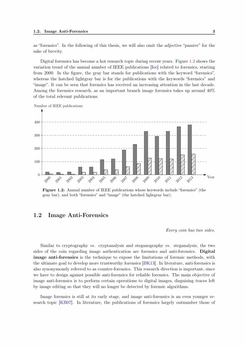
Digital forensics has become a hot research topic during recent years. Figure 1.2 shows thevariation trend of the annual number of IEEE publications [Iee] related to forensics, startingfrom 2000. In the figure, the gray bar stands for publications with the keyword “forensics”,whereas the hatched lightgray bar is for the publications with the keywords “forensics” and“image”. It can be seen that forensics has received an increasing attention in the last decade.Among the forensics research, as an important branch image forensics takes up around 40%of the total relevant publications.
Year
Number of IEEE publications
0
100
200
300
400
2000
2001
2002
2003
2004
2005
2006
2007
2008
2009
2010
2011
2012
2013
Figure 1.2: Annual number of IEEE publications whose keywords include “forensics” (thegray bar), and both “forensics” and “image” (the hatched lightgray bar).
1.2 Image Anti-Forensics
Every coin has two sides.
Similar to cryptography vs. cryptanalysis and steganography vs. steganalysis, the twosides of the coin regarding image authentication are forensics and anti-forensics. Digitalimage anti-forensics is the technique to expose the limitations of forensic methods, withthe ultimate goal to develop more trustworthy forensics [BK13]. In literature, anti-forensics isalso synonymously referred to as counter-forensics. This research direction is important, sincewe have to design against possible anti-forensics for reliable forensics. The main objective ofimage anti-forensics is to perform certain operations to digital images, disguising traces leftby image editing so that they will no longer be detected by forensic algorithms.
Image forensics is still at its early stage, and image anti-forensics is an even younger re-search topic [KB07]. In literature, the publications of forensics largely outnumber those of
4 Chapter 1. Introduction
anti-forensics. Moreover, existing anti-forensic methods often use simple image processing todisguise traces left by a targeted operation, e.g., using filtering to hide compression artifacts[SL11], or using noise addition to disguise footprints left by filtering [WSL13]. Indeed, suchanti-forensic methods can be very successful in defeating the targeted forensic detectors, butcan also be easily exposed by more advanced detectors. Moreover, the anti-forensic image gen-erated by these methods often suffers from a low visual quality. This is a worrying issue, sincean image of low quality (e.g., a blurry/noisy image) may spontaneously rouse the suspicion ofits authenticity.
In summary, image anti-forensics has a two-fold end: a good forensic undetectability aswell as a high visual quality of the processed image [KR08]. Between these two goals, theforensic undetectability is more important than the image quality for image anti-forensics.Anti-forensics cannot claim to be successful if there exist a certain detector which is able todetect the anti-forensic images.
1.3 Objectives and Contributions
In this thesis, we stand on the image anti-forensic side, with the focus on JPEG (Joint Pho-tographic Experts Group) compression and median filtering anti-forensics. From a JPEGcompressed or median filtered image, if we can successfully create a “fake” image that ap-pears never processed, it would be a relatively easy task to conduct image processing historyfalsification or even tampering afterwards. To this end, we employ some frameworks fromimage restoration field meanwhile integrating some anti-forensic terms/strategies, for creatinganti-forensic images with a good tradeoff between forensic undetectability and image quality.
1.3.1 JPEG Compression and Median Filtering
Firstly, we choose to conduct our research on image anti-forensics to JPEG compression,because JPEG is probably the most common image format in use today on Internet, and canbe easily found in various forensic scenarios. According to the statistics of the usage of imagefile formats for websites on December 8, 2014, JPEG is the most widely used one, with theusage by 68.7% of all the websites [W3t].
We can imagine the following forgery creation scenario involving JPEG compression, asillustrated in Figure 1.3. In order to make people believe that someone has participated ina certain event, the forger will probably create a composite with the scene and the personfrom two JPEG images with different quality factors3. The resulting image is likely to beJPEG compressed again before publishing. Careful image editing may leave no visual cluesnoticeable by human naked eyes, yet the forgery can be exposed by detecting different kindsof double JPEG compression artifacts present in different areas of the image [BP12b].
3The quality factor is an integer between 1 and 100. The greater the quality factor is, the higher the qualityof the compressed image is, and the larger the JPEG file will be. A more detailed description of the qualityfactor can be found in Section 3.1.1.

1.3. Objectives and Contributions 5
Figure 1.3: Illustration of creating a composite JPEG image. Here q1, q2 and q3 are threepossibly different quality factors for JPEG compression.
Generally speaking, the goal of JPEG anti-forensics is to remove all possible footprints left
by JPEG compression, so that the resulting anti-forensic JPEG image looks as if it were anoriginal uncompressed one. Now, count for the possibility that a smart forger employs JPEGanti-forensics to hide JPEG compression artifacts of the two source JPEG images so thatthey seem never compressed. Therefore, no (different types of) JPEG compression artifactsindicating image manipulation will appear in the composite image forgery. Thereafter, theimage can be re-compressed using another compression setting, so as to either hide traces ofdouble JPEG compression, or falsify the image origin, or serve for other possible anti-forensicpurposes [SL11].
In the very recent work of JPEG anti-forensics [SL11] as well as the image resampling anti-forensics conducted in [KR08], median filtering shows its destructive nature to other imageprocessing footprints. However, the median filter, as a well-known and widely used imagedenoising and smoothing operator, leaves trackable clues in the image. They can be detectedby various median filtering forensic detectors. The presence of median filtering traces, not onlysuggests the image has been previously median filtered, but also implies the possibility thatother image processing operations may have been applied to the image. Hence, it is of greatsignificance to conduct median filtering anti-forensics, which constitutes the second researchsubject of this thesis.

6 Chapter 1. Introduction
1.3.2 Image Anti-Forensics and Image Restoration
When it goes to image coding or processing, we notice that image anti-forensics to some extentshares a similar goal to image restoration, which is to recover the information lost during theimage degradation, via solving an ill-posed inverse problem. Indeed, for certain anti-forensicscenarios, e.g., attacking physically based or geometric-based forensic algorithms (see Sec-tion 2.1.1 for their brief descriptions), this similarity no longer holds. However, their relevantanti-forensic study is beyond the scope of this thesis, and we mainly focus on JPEG com-pression and median filtering anti-forensics here. The objective of image restoration usuallygoes to the visual quality improvement of degraded images. While image anti-forensics hopesto recover the underlying statistics of the original, genuine image to the utmost, so that theresulting image forgery appears to be authentic. High visual quality of the processed imageis certainly one important goal of image anti-forensics. Besides, it is also worth noticing thatimage anti-forensics has an additional indispensable goal, i.e., a good forensic undetectability,compared with image restoration.
Given the similarities between image anti-forensics and image restoration, this thesis aimsto generate, from a JPEG compressed or median filtered image, a “natural” image whichappears to be never processed. To this end, the maximum a posteriori (MAP) estimation(or one of its variants) is employed. Under this framework, several different natural imagestatistical models from image restoration are adopted and enriched by integrating some anti-forensic terms/strategies concerning the forensic undetectability. In order to solve differentproposed image anti-forensic problems, several numerical optimization methods are used. Bydoing so, we hope to be able to estimate the “best” anti-forensic image in some sense. Atlast, the anti-forensic images, with a good tradeoff between forensic undetectability and imagequality, are generated.
1.3.3 Methodology
Different from the state-of-the-art JPEG/median filtering anti-forensics work based on simpleimage processing [SL11, WSL13], here a new research line is proposed to conduct imageanti-forensics. In this thesis, we propose sophisticated digital image anti-forensic methodsto JPEG compression and median filtering, leveraging on advanced concepts and tools fromimage restoration, natural image statistics and numerical optimization.
The blocking artifacts in the spatial domain and the quantization artifacts in the DCT(Discrete Cosine Transform) domain of one image are both evidence of JPEG compression[FD03]. In this thesis, the following methods are developed for JPEG anti-forensic purposes:
• Firstly, a constrained Total Variation (TV) based minimization [ADF05] is employed forremoving the JPEG blocking artifacts. Moreover, in order to ensure the visual qualityof the final obtained anti-forensic JPEG image, a modified Quantization Constraint Set(QCS) projection [RS05] is used.

1.4. Outline 7
• For the quantization artifacts in the DCT domain, a perceptual DCT histogram smooth-ing method is proposed based on the local Laplacian model and the partly recoveredDCT-domain information obtained after applying the TV-based deblocking.
• Furthermore, in order to study the impact of a more advanced image prior model to theJPEG anti-forensics task, the Gaussian Mixture Model (GMM) for overlapping imagepatches [ZW11] and a likelihood term modeling the JPEG compression process [RS05]are considered. Besides, we also propose a new, non-parametric method to DCT his-togram smoothing based on calibration [FGH02].
As to median filtering anti-forensics, this thesis proposes an image variational deconvo-lution framework, inspired by the literature on image deconvolution [KF09, KTF11]. Thisoptimization-based framework consists of a convolution term approximating the median fil-tering process, a fidelity term with respect to the median filtered image, and an image priorterm based on the generalized Gaussian distribution in the pixel value difference domain.
In order to validate the efficiency of the proposed JPEG/median filtering anti-forensicmethods, large-scale forensic tests are carried out. Experimental results demonstrate thatthe proposed methods outperform the state-of-the-art anti-forensics, with a better forensicundetectability against existing forensic detectors as well as a higher visual quality of theanti-forensic image.
1.4 Outline
The remainder of this thesis4 is organized as follows.
Chapter 2 presents some background knowledge on image forensics and anti-forensics,including the classification, evaluation metrics, natural image datasets used in forensic testingof this thesis, and relevant optimization methods which will be used in the proposed imageanti-forensic methods.
Chapter 3 reviews the state-of-the-art image forensic algorithms and anti-forensic methodsto JPEG compression and median filtering. The reviewed forensic algorithms are the attackingtargets of the proposed anti-forensic methods, while the reviewed anti-forensic methods areused for experimental comparisons.
Chapter 4 proposes a JPEG deblocking method, by optimizing a constrained TV-basedminimization problem, whose cost function is composed of a TV term and a TV-based block-ing measurement term. Besides a good deblocking effect, the resulting anti-forensic JPEG
4In this thesis, most of the contents in Chapters 4-7 were published or have been accepted for publicationin international conferences or international journals. As to JPEG anti-forensics, we published three papers[Fan+13a, Fan+14, Fan+13b] where different divisions of datasets, compression quality factors and evaluationmetrics were used. For consistency consideration of the thesis, we will use the same setting (see Sections 2.2and 2.3 for details) across Chapters 4-6. Therefore, the relevant figures and tables may not be exactly thesame, but should be in accordance with those shown in our published papers.

8 Chapter 1. Introduction
image also achieves relatively good forensic undetectability even against quantization artifactsdetectors. Yet, the DCT-domain quantization artifacts still to some extent exist, which maybe used by potential forensic detectors. Therefore, this method will be further improved inChapter 5.
Chapter 5 describes an improved JPEG anti-forensic method based on the work in Chap-ter 4 yet with a different parameter setting. The remaining comb-like quantization artifactsin the TV-based deblocked JPEG image are explicitly filled by a perceptual DCT histogramsmoothing procedure.
Chapter 6 presents a JPEG quality enhancement method based on an MAP-based frame-work using the GMM as the image prior model for the overlapping image patches. ForJPEG anti-forensic purposes, the DCT histogram smoothing is performed using a new, non-parametric method based on calibration.
Chapter 7 proposes a median filtered image quality enhancement approach as well as amedian filtering anti-forensic method, by approximating the median filtering process usingimage convolution and by using the generalized Gaussian to model the pixel value difference.
Chapter 8 concludes this thesis, by summarizing the contributions and proposing severalperspectives about the future research work on digital image anti-forensics.

Chapter 2
Preliminaries
Contents2.1 Classification of Image (Anti-)Forensics . . . . . . . . . . . . . . . . . . 10
2.1.1 Farid’s Classification of Image Forensics . . . . . . . . . . . . . . . . . . . 10
2.1.2 Redi et al.’s Classification of Image Forensics . . . . . . . . . . . . . . . . 10
2.1.3 Piva’s Classification of Image Forensics . . . . . . . . . . . . . . . . . . . 11
2.1.4 Stamm et al.’s Classification of Image Forensics . . . . . . . . . . . . . . . 12
2.1.5 Böhme and Kirchner’s Classification of Image Anti-Forensics . . . . . . . 13
2.1.6 Classification of Proposed Anti-Forensic Methods . . . . . . . . . . . . . . 14
2.2 Evaluation Metrics . . . . . . . . . . . . . . . . . . . . . . . . . . . . . . 14
2.2.1 Forensic (Un)detectability . . . . . . . . . . . . . . . . . . . . . . . . . . . 15
2.2.1.1 Scalar-Based Detectors . . . . . . . . . . . . . . . . . . . . . . . 17
2.2.1.2 SVM-Based Detectors . . . . . . . . . . . . . . . . . . . . . . . . 18
2.2.2 Image Quality . . . . . . . . . . . . . . . . . . . . . . . . . . . . . . . . . 21
2.2.2.1 PSNR . . . . . . . . . . . . . . . . . . . . . . . . . . . . . . . . . 21
2.2.2.2 SSIM . . . . . . . . . . . . . . . . . . . . . . . . . . . . . . . . . 21
2.2.3 Histogram Recovery . . . . . . . . . . . . . . . . . . . . . . . . . . . . . . 22
2.3 Natural Image Datasets . . . . . . . . . . . . . . . . . . . . . . . . . . . 22
2.3.1 JPEG Forensic Testing . . . . . . . . . . . . . . . . . . . . . . . . . . . . . 22
2.3.2 Median Filtering Forensic Testing . . . . . . . . . . . . . . . . . . . . . . 24
2.4 Relevant Optimization Algorithms . . . . . . . . . . . . . . . . . . . . . 25
2.4.1 Subgradient Method . . . . . . . . . . . . . . . . . . . . . . . . . . . . . . 25
2.4.2 Hungarian Algorithm . . . . . . . . . . . . . . . . . . . . . . . . . . . . . 26
2.4.3 Half Quadratic Splitting . . . . . . . . . . . . . . . . . . . . . . . . . . . . 27
2.4.4 Split Bregman Method . . . . . . . . . . . . . . . . . . . . . . . . . . . . . 28
This chapter firstly presents the basic knowledge of digital image forensics and anti-forensics, including the classification and evaluation metrics. After that, the natural
images datasets used in the forensic testing of this thesis are introduced. Finally, we brieflyreview the optimization algorithms which will be used for solving the optimization problemsproposed in this thesis.
9
10 Chapter 2. Preliminaries
2.1 Classification of Image (Anti-)Forensics
2.1.1 Farid’s Classification of Image Forensics
Digital image forensics makes the assumption that the forgery creation process has disturbeda certain kind of intrinsic scene/image properties (e.g., statistical, physical or geometricalproperties). In this context, Farid [Far09a] groups digital image forensics into the followingfive categories:
• Pixel-based image forensics analyzes pixel-level anomalies caused by image tampering.Some frequently used image manipulation means are, for instance, copy-and-paste, splic-ing, resampling and median filtering. Targeting at each of these image operations, vari-ous forensic techniques are proposed.
• Format-based image forensics detects the image statistical change introduced by a certainlossy compression method. Popular image compression algorithms include JPEG basedon the DCT transform, SPIHT (Set Partitioning In Hierarchical Trees) and JPEG2000based on the wavelet transform, etc.
• Camera-based image forensics studies digital image ballistics [Far06] from the imagingstage inside the camera. Typical forensic methods in this category are for instancebased on the chromatic aberration, the color filter array (CFA), the photo responsenon-uniformity (PRNU) noise, etc.
• Physically based image forensics examines anomalies of interaction between objects,light, and the camera in the 3-dimensional physical world. For example, the consis-tencies of light direction or of lighting environment estimated from different physicalobjects can be used as criteria for forensic purposes.
• Geometric-based image forensics measures the positions of physical objects with respectto the camera. For instance, image tampering can be detected if across the image thereexist inconsistencies in the principal point5.
Despite that [Far09a] mainly reviews image forensics, Farid also points out that new techniques(i.e., anti-forensics) will be developed to create fake images which are harder to be detected.The arms race between forensic analysts and forgers is inevitable.
2.1.2 Redi et al.’s Classification of Image Forensics
In [RTD11], Redi et al. review image forensic methods in the following two categories:
5The principal point is the projection of the camera center onto the image plane.

2.1. Classification of Image (Anti-)Forensics 11
• Image source device identification is to identify the device which is used for the acquisi-tion of the given image. Relevant source identification methods can be further groupedinto the following three subcategories:
– Identification through artifacts produced in the acquisition phase, such as forensicmethods based on the chromatic aberration, the CFA, etc.
– Identification through sensor imperfections, such as forensic methods based on pixeldefects, the fixed pattern noise (FPN), the PRNU, etc.
– Source identification using properties of the imaging device, such as forensic meth-ods based on the color processing, the JPEG compression, etc.
• Tampering detection is to expose the intentional image manipulation which modifies thesemantic meaning of the image. Relevant tampering detection methods can be furthergrouped into the following three subcategories:
– Detecting tampering performed on a single image, in one of the most common ways,is to expose the copy-move of a region within an image. Some relevant knownforensic methods leverage on the tools such as the principal component analysis(PCA), the scale-invariant feature transform (SIFT), etc.
– Detecting image composition, in other words, is to expose image splicing. Incon-sistencies of certain properties across different parts of the image can all serve asevidence of tampering, such as the light direction, the complex lighting environ-ment, shadows/reflections of objects, the PRNU, the JPEG compression, etc.
– Tampering detection independent on the type of forgery, is a general technique whichcovers both tampering involving a single image and tampering involving multipleimages. In order to realize this general forensic method, possible ways are to exploitthe resampling traces, compression artifacts, acquisition device fingerprints, etc.
Meanwhile, Redi et al. [RTD11] also point out that image anti-forensics is the new phase fordeveloping new and more powerful forensic methods.
2.1.3 Piva’s Classification of Image Forensics
In [Piv13], Piva surveys digital image forensics according to the image life cycle, which aredivided into three stages: image acquisition, image coding, and image editing. Digital imageforensics can therefore be divided into the following three categories:
• Acquisition footprints based image forensics. When a digital image is recorded by acamera, each imaging stage introduces intrinsic footprints due to the imperfection of thedevice (e.g., PRNU noise caused by the image sensor) or because of the different cameramanufacturer choices in both the hardware (e.g., different lens leading to different chro-matic aberration parameters) and software (e.g., different CFA configurations). Theseimage artifacts vary according to different camera brands and/or models, and can be

12 Chapter 2. Preliminaries
considered as the signature of a specific camera type (i.e., the so-called image ballistics
defined in literature [Far06]). Inconsistencies in these footprints across the image can beconsidered as evidence of tampering.
• Coding footprints based image forensics. Lossy compression is widely used to reduceimage redundancy for efficiently storing and transmitting the data. Different codingarchitectures leave different telltale footprints, which can be used for image forensicpurposes. In literature, JPEG compression probably draws the most attention in thiscategory. Researchers also notice that artifacts present in a single JPEG compressedimage (i.e., compressed only once) will vary when the JPEG compression is appliedagain. Image manipulation can therefore be exposed when inconsistencies of codingfootprints are detected.
• Editing footprints based image forensics. Careful image editing may not leave visualtraces, yet will probably disturb the intrinsic properties of the authentic image. There-fore, inconsistency/deviation of these intrinsic properties across the image can be con-sidered as evidence of tampering.
Besides, Piva also provides a brief review and discussion concerning image anti-forensics in[Piv13], based on Böhme and Kirchner’s [BK13] classification of image anti-forensics (to bedescribed in Section 2.1.5). Almost all the existing image anti-forensic methods are designedto target one particular forensic tool. Conversely, universal anti-forensics aims to maintainimage statistics which are not known to the image forger. It is certainly a more difficultproblem and an interesting open research question, but should be able to escape the eternalloop between targeted forensics and anti-forensics.
2.1.4 Stamm et al.’s Classification of Image Forensics
Stamm et al. [SWL13] review the information forensics in the last decade. Concerning imageforensics, the following two aspects are discussed in detail:
• Detection of tampering and processing operations. In many scenarios, the processinghistory of the image is one of the primary concerns to determine whether it can betrusted. This can be identified by exploiting intrinsic properties of the digital content.Relevant forensic techniques can be further divided into the following five subcategories:
– Forensics based on statistical classifiers;
– Forensics detecting device fingerprints;
– Forensics exposing manipulation fingerprints;
– Forensics examining compression and coding fingerprints;
– Forensics checking physical inconsistencies.
• Device forensics. Digital images have seen a huge growth because of the advancementof digital cameras. Identifying the acquisition device of an image is an important step

2.1. Classification of Image (Anti-)Forensics 13
to ensure the security and trustworthiness. Relevant forensic techniques can be furtherdivided into the following four subcategories:
– Forensics exploring color processing traces;
– Forensics linking to individual device units;
– Forensics identifying imaging type;
– Forensics detecting manipulation using device fingerprints.
Meanwhile, Stamm et al. [SWL13] also present a brief overview of some current image anti-forensic work. More specifically, there exist image anti-forensic techniques based on PRNU,resampling, compression, etc.
2.1.5 Böhme and Kirchner’s Classification of Image Anti-Forensics
In [BK13] Böhme and Kirchner divided image anti-forensic techniques into two categoriesalong the following three dimensions, respectively:
• Robustness vs. Security. In general, image forgers can exploit robustness or securityweaknesses of image forensics for anti-forensic purposes.
– The robustness of image forensics is its reliability under legitimate post-processing.For instance, many forensic algorithms (lighting-based forensics is a good exampleof exception here) fail when strong JPEG compression is applied. Such legitimatepost-processing can serve as an anti-forensic technique, as long as it is able to movethe plausible forgeries outside the detection region of the forensic detectors.
– The security of image forensics shows how much it is able to expose intentionallyconcealed illegitimate post-processing. That is to say, the security indicates theability to withstand anti-forensics. Image forgers can exploit the weaknesses of theimage model used by forensics. This more powerful anti-forensic attack createsimage forgeries which are moved in a particular direction outwards the decisionregion of the authentic images.
• Post-Processing and Integrated Attacks.
– Post-Processing anti-forensic attacks edit the image, as an additional processingstep, such that it does not leave traces which can be detected by image forensics.
– Integrated anti-forensic attacks directly interfere the image generation process.They do not address the robustness of image forensics, by definition.
• Targeted and Universal Attacks.
– If the anti-forensic method exploit the weaknesses of a specific forensic tool, it istargeted. It is possible for this kind of anti-forensics to be detected by other forensicalgorithms using alternative/improved image models.

14 Chapter 2. Preliminaries
– Universal anti-forensic attacks try to create image forgeries whose statistical prop-erties are maintained as much as possible, so the fake images remain undetectableeven when examined by unknown forensic tools. This is clearly a more difficulttask and an interesting open research problem. The main difficulty here is whetherwe can find a good enough image model which is able to resist combined analysisof forensic algorithms.
2.1.6 Classification of Proposed Anti-Forensic Methods
In this thesis, from the image restoration field, we borrow some MAP (or one of its variants)based frameworks meanwhile integrating some anti-forensic terms/strategies concerning theforensic undetectability, in order to cope with the anti-forensics problems to JPEG compressionand median filtering. According to Farid’s classification [Far09a] of digital image forensics,JPEG forensics is format-based, whereas median filtering forensics is pixel-based. Based onRedi et al.’s classification [RTD11], JPEG compression can be involved in both source identi-
fication and tampering detection, and median filtering forensics belongs to tampering detection.According to Piva’s classification [Piv13], JPEG forensics analyzes the coding footprints, whilemedian filtering forensics detects editing footprints. However, for both JPEG and medianfiltering forensic techniques, they detect tampering and processing operations [SWL13]. Morespecifically, JPEG forensics examines compression and coding fingerprints, and median filteringforensics exposes manipulation fingerprints. According to Böhme and Kirchner’s classification[BK13] of image anti-forensics, the proposed JPEG and median filtering anti-forensic methodsare post-processing/targeted attacks analyzing the security of forensic algorithms.
2.2 Evaluation Metrics
As noted in Chapter 1, image anti-forensics has a two-fold goal: a good forensic undetectabilityand a high visual quality of the anti-forensic image. Forensic undetectability (on the anti-forensic side) is a metric versus forensic detectability (on the forensic side). Both of themcan be measured by analyzing the ROC (Receiver Operating Characteristic) curve (to bedescribed in Section 2.2.1). Good forensic undetectability means good performance of the anti-forensic method, and poor performance of the forensic algorithm. Conversely, good forensicdetectability means poor performance of the anti-forensic method, and good performance ofthe forensic algorithm.
Image anti-forensics consists in creating visually plausible fake images. Indeed, the forensicundetectability is the priority objective of image anti-forensics. Meanwhile, the visual qualityis also an important factor to evaluate the anti-forensic performance, since the low qualityimage may spontaneously rouse the concerns of its authenticity. The image quality evaluationcan be performed by using the well-known PSNR (Peak Signal-to-Noise Ratio) and SSIM(Structural SIMilarity) metrics described in Section 2.2.2.
2.2. Evaluation Metrics 15
Besides, JPEG/median filtering anti-forensics often involves certain histogram recovery(see Sections 5.3.1 and 7.3.4 for details). In order to evaluate the histogram restoration,we adopt the Kullback-Leibler divergence [KL51] (in short, KL divergence), which will bedescribed in Section 2.2.3.
2.2.1 Forensic (Un)detectability
In most forensic scenarios, digital image forensics builds a binary classifier6. Given a digitalimage, the forensic detector makes a decision to say that it is either genuine or fake. In otherwords, the main objective of digital image forensics is to establish a detector, which is able todifferentiate genuine images from image forgeries with a high detection accuracy. In this thesis,we study JPEG compression and median filtering and try to disguise the compressed/filteredimage as never processed. Here, the genuine image refers to the original, unprocessed image.Whereas the image forgery refers to the processed image, more specifically, the (anti-forensic)JPEG image described in Chapters 4-6, and the (anti-forensic) median filtered image describedin Chapter 7.
The performance of a forensic algorithm or an anti-forensic method can be evaluated bycomparing the forensic detector’s classification outcome obtained on a set of images with theground-truth. Let us consider a forensic testing with NN genuine images (i.e., the unprocessedimages, here considered as negative samples) and NP fake images (i.e., the processed images,here considered as positive samples). Among the NN negative samples, let NFP denote thenumber of negative samples which are falsely classified as positive. Among the NP positivesamples, let NTP denote the number of positive samples which are correctly classified aspositive. For each classification strategy of a forensic detector, a false positive rate (RFP ) anda true positive rate (RTP ) can therefore be calculated as follows:
RFP =NFP
NN, RTP =
NTP
NP. (2.1)
With (RFP , RTP ) pairs obtained by different classification strategies of a forensic detector,a ROC curve can be plotted in the ROC space. The final classification strategy is determinedby analyzing this ROC curve. Usually it is required that the false positive rate should not betoo high. In layman’s terms, we should not wrong an innocent person (i.e., classify a genuineimage as fake in digital image forensics), which is critical in some scenarios such as the lawenforcement. Under this criterion, the detector chooses the ROC point corresponding to thebiggest true positive rate with the constraint that the false positive rate is smaller than acertain threshold. In this context, many anti-forensic methods aim to lower the true positiverate of a detector when the false positive rate is below a certain threshold. Yet, the morecomprehensive way is still to analyze the trend of the whole ROC curve.
Figure 2.1-(a) illustrates the ROC space, which is defined by false positive rate RFP and
6Indeed, in certain forensic cases, e.g., image source identification, may require a multi-class classifier.However, it is beyond the scope of this thesis and will not be discussed here.

16 Chapter 2. Preliminaries
true positive rate RTP as x and y axes respectively. If the upper-left point (0, 1) in the ROCspace is included in a ROC curve, it indicates that the corresponding forensic detector isable to achieve the so-called perfect classification. In this case, the detector can successfullydiscriminate between genuine and fake images without any error. This is ideal for forensics,yet very hard to achieve in practice. In general, the goal of the forensic detector is to dragthe ROC curve towards the perfect classification point of the ROC space to the utmost. Anexample can be seen at point A in Figure 2.1-(a). Here, the forensic detector is able to achievea relatively high true positive rate with a relatively low false positive rate.
False positive rate
Truepositiverate
0 0.2 0.4 0.6 0.8 10
0.2
0.4
0.6
0.8
1Random guess
perfect classification
A
B
C
(a) ROC space
False positive rate
Truepositive
rate
0 0.2 0.4 0.6 0.8 10
0.2
0.4
0.6
0.8
1
Random guess
(b) ROC curve
Figure 2.1: The ROC space and an example of ROC curve.
On the anti-forensic side, the forger hopes to create image forgeries so that the ROC curveachieved by a forensic detector is close to the diagonal line (i.e., the random guess line) ofthe ROC space. In this case, the detector is not able to tell the image forgeries from thegenuine images even when the “best” classification strategy is used. For example, at point Bin Figure 2.1-(a), the detector’s classification outcome is equivalent to a random guess. Thatis to say, given any image, the chances of the detector saying it is either genuine or fake areequal. It is equivalent to randomly deciding whether a given image is genuine/fake. This isthe worst classification outcome of a detector. Statistically, the forensic features of the genuineimages and of the image forgeries are well mixed together, which are non-distinguishable bythe forensic detector.
The point C in Figure 2.1-(a) indicates that the detector achieves a quite low true positiverate at a quite high false positive rate. In this case, the classification outcome appears to beeven worse than that of point B on the random guess line. Yet, this does not imply that theforensic feature is not well designed. Conversely, it indicates that the classification strategyis not appropriate. This issue can be resolved by simply flipping the classification strategy,i.e., classifying the image deemed as forgery in the original classification strategy as genuine,meanwhile classifying the image deemed as genuine image in the original classification strategyas fake. Therefore, the ROC point in the bottom right corner of the ROC space will switch

2.2. Evaluation Metrics 17
to the top left corner.
With multiple ROC points, a ROC curve can be plotted in the ROC space. An examplecan be found in Figure 2.1-(b). It is more comprehensive to analyze the trend of the wholeROC curve than a single ROC point, for evaluating the forensic undetectability of the anti-forensic method or the forensic detectability of the forensic algorithm. For a quantitativeevaluation, we use the popular AUC (area under curve) metric, by measuring the area underthe ROC curve. The AUC value varies in the range [0, 1]. When the AUC value is close to1, it means that the ROC curve is close to the perfect classification point of the ROC space,indicating a good forensic detectability and a poor forensic undetectability. When the AUCvalue is close to 0.5, it means that the ROC curve is close to the random guess line, indicatinga good forensic undetectability and a poor forensic detectability. When the AUC value is closeto 0, it means that the ROC curve is close to the bottom-right point of the ROC space. Thisdoes not really mean that the forensic detectability of the detector is poor. As stated above,the AUC value can reach close to 1 when the classification strategy is flipped.
The forensic testing requires a set of images including both genuine and fake images, aswell as a forensic detector. In the forensic experimental setting of this thesis, certain imagedataset (described in Section 2.3) containing genuine images is used. For each genuine image,it is processed to generate a corresponding image forgery. At last, an equal number of genuineimages and image forgeries are used for forensic testing. On the other hand, the feature of aforensic algorithm can be either a scalar or a vector, depending on the specific method. Theircorresponding forensic tests are to some extent different. In the image forensics literaturewhere the feature is vector-based, it is a common practice to adopt the SVM (Support VectorMachine) for training the forensic detector. In Sections 2.2.1.1 and 2.2.1.2, we will describehow to conduct the forensic test for forensic (un)detectability evaluation, using scalar-baseddetectors and SVM-based detectors, respectively.
2.2.1.1 Scalar-Based Detectors
Given an image, the scalar-based forensic algorithm outputs a feature value. The forensicdetector classifies the image as either genuine or fake, by comparing this feature value witha pre-defined threshold. If the feature value is greater (or smaller) than the threshold, theimage is classified as fake. Otherwise, the image is classified as genuine.
The threshold can vary, thereafter producing different classification outcomes. Then dif-ferent classification strategies of the detector are defined by different thresholds. Indeed, thethreshold can be defined as any value. In the experiments of forensic testing, the common prac-tice is as follows. The detector outputs the feature value for each image under examination.Then, all these obtained feature values (or their uniformly sampled values) are used as thedifferent thresholds for producing different classification strategies of the detector. Thereafter,a ROC curve can be plotted and an AUC value can be calculated.

18 Chapter 2. Preliminaries
2.2.1.2 SVM-Based Detectors
Many forensic features are vector-based. In the image forensics literature, probably the mostcommon way to build a forensic detector based on a vector-based feature is to use a two-classSVM7. In this thesis, we follow this common practice of adopting the SVM in image forensics.
For the feature vectors computed from the positive and negative samples, the SVM builds amaximum-margin hyperplane that achieves the largest distance to the nearest training featurevector of either of the two classes. On the two sides of the separating hyperplane, two parallelsupporting hyperplanes are selected in a way that there are no feature vectors between them(namely, hard margin) and their distance is maximized. The region bounded by these twohyperplanes is the so-called “margin”. The feature vectors on the margin are, namely, the“support vectors”.
In practice, it happens that certain training samples are mislabeled, i.e., some positivesamples are labeled negative, or some negative samples are labeled positive. In order to controlthe sensitivity of the SVM to noisy data, the so-called soft-margin method (with respect tothe hard-margin one described earlier) is introduced. It allows that a few training samples fallinto the margin but are on the correct side of the separating hyperplane, or that some trainingsamples are even on the wrong side of the separating hyperplane. For the soft-margin SVM,the degree of misclassification of the data is penalized by the parameter C.
It often happens that the positive and negative samples are not linearly separable in thefeature space. To cope with this problem, the so-called kernel trick is introduced to implicitlymap the feature vectors into a higher-dimensional space, where hopefully the separation iseasier. This trick makes the SVM very powerful to perform non-linear classifications, andtherefore bring its popularization in various classification applications. Some widely usedkernels include, the Gaussian kernel (also known as the Radial Basis Function (RBF) kernel),the polynomial kernel, the sigmoid kernel, etc.
In the image forensics literature where the feature is vector-based, the soft-margin SVMwith the following Gaussian kernel is often used:
k(φ,ψ) = exp(−γ||φ−ψ||22), γ > 0, (2.2)
where φ and ψ are two feature vectors, and γ is the kernel parameter. To follow the commonpractice in image forensics literature, this thesis keeps the above choice of using soft-marginSVM with Gaussian kernel so as to build the SVM-based forensic detector, when the forensicfeature is vector-based.
The penalization parameter C and the kernel parameter γ (interested readers can referto [CL11] for more details) need to be determined before the SVM classifier is trained. Thecomplexity and accuracy of the SVM classifier are balanced by the parameter setting of (C, γ).Pevný et al. [PBF10] have discussed the impact of different values of C and γ to the SVM
7In the following, we omit the word “two-class” for describing the SVM, for the sake of brevity. Here, wedo not consider multi-class SVM. The SVMs we use in this thesis are all two-class.

2.2. Evaluation Metrics 19
classifier in detail. High value of C can improve the accuracy of the classifier on the trainingdataset but also increases the complexity. On the contrary, low value of C decreases theaccuracy of the classifier but can normally achieve a good generalization with low complexity.Similarly, high value of γ may cause the over-fitting problem of the classifier, while low valueof γ has the opposite impact.
The parameter setting of (C, γ) should well balance both the accuracy and complexity ofthe SVM classifier. In order to choose proper values for them, the standard way is to carryout a grid search with cross-validation. In this thesis, we follow the suggestion in [PBF10] anduse the five-fold cross-validation with the following multiplicative grid:
C ∈ {0.001, 0.01, · · · , 10000}γ ∈
{
2i | i ∈ {−log2D − 3, · · · ,−log2D + 3}}
,(2.3)
where D is the dimensionality of the feature vector. In this thesis, we use the LIBSVM library[CL11] to train and test the SVM-based forensic detectors.
In this thesis, we consider some forensic feature which can be as high as 686-dimensional(i.e., the KS686
SPAM in Table 3.3). However, for the forensic testing of both JPEG compressionand median filtering, we “only” use 500 samples (the datasets used for forensic testing areto be described in Sections 2.3.1 and 2.3.2) for each of the positive and negative classes fortraining the SVM classifiers. Fortunately, the SVM is by concept a classifier designed to be lesssensitive to the problem of curse of dimensionality. As pointed out by Vapnik [Vap98], “Onecan consider the SV technique as a new type of parameterization of multidimensional functionsthat in many cases allows us to overcome the curse of dimensionality.” (Note: here the “SV”stands for the “Support Vector”.) In fact, the SVM appears to be especially advantageouswhen there are only a few training samples available and the feature is high-dimensional, ascenario rather quite frequently encountered in practical applications. This is mainly becauseof the fact that the classification strategy of the SVM is based on maximizing the margin inan implicit higher-dimensional space. This “geometrical” nature of the SVM does not requirean estimation of the statistical distributions of classes, leading to a good generalization evenwhen there are only limited number of training samples [MB04].
Steganography is the art of embedding secret message into an image, a video, or otherforms of data. It is another domain in multimedia security field, which is different from anti-forensics but shares some common goals with anti-forensics [BK13]. In one of the most recentsteganography work [HF13], the undetectability of the stego-images becomes poor when thepayload reaches 0.5 bpp (bits per pixel).
It is a popular way to create image forgeries by compositing two images. An example in-volving JPEG compression is illustrated in Figure 1.3. Inspired by this common practice, weuse a similar experimental setup to steganalytic testing, in order to conduct forensic testingusing SVM-based detectors. As illustrated in Figure 2.2, for a given genuine, unprocessedimage, the center part of the image is replaced by its corresponding processed image (JPEGcompressed/median filtered, or processed again using anti-forensic methods) with a replace-ment rate around the values in {0.05, 0.1, 0.15, 0.2, 0.3, 0.4, 0.5, 0.6, 0.8, 1} to create the image

20 Chapter 2. Preliminaries
forgery. For each replacement rate, the resulting composite image forgeries and the originalimages are then mixed together for training and testing the SVM-based detectors. Here, theimage replacement rate in forensic testing can be taken as a counterpart of the bpp in imagesteganography.
Figure 2.2: Illustration of creating a composite image forgery for training/testing theSVM-based detector.
Given an SVM-based detector and a set of images for forensic testing, a decision value isoutput by the SVM for each image. Similar to the scalar-based detectors, different classifica-tion strategies are implemented by varying the thresholds for the decision values. Thereafter,a ROC curve is plotted and an AUC value is calculated.
The SVM-based detectors are built based on the assumption that the forensic investigatorhas the knowledge of the anti-forensic method and is able to create a large amount of imageforgeries for training the detector. This is standing on the beneficial side for forensics and isthe worst-case scenario for anti-forensics. In practice, we also find it very difficult to disguise awhole processed (JPEG compressed or median filtered in this thesis) image as never processed,when examined under an SVM-based detector under this worst-case scenario. Currently, thereare no JPEG or median filtering image anti-forensic algorithms which are able to fool powerfulSVM-based detectors. This can be reflected by high AUC values when the replacement rateis close to 1 (Please see Sections 5.3.2, 7.3.4 and 7.4 for detailed experimental results). Thisobservation in practice backs the statement of [BK13]: it is a challenging task to developanti-forensic methods capable of resisting machine learning based detectors.
Standing on the anti-forensic side, this thesis mainly considers the results obtained witha relatively low replacement rate. We remain reserved on the undetectability of a wholeimage generated by anti-forensics. However, it can still find many applications in various anti-

2.2. Evaluation Metrics 21
forensic scenarios, e.g., image splicing and tampering with relatively low replacement rate. Forexample, an image forgery can be created by replacing the head of one person in the picturewithout being detected.
2.2.2 Image Quality
The image quality assessment methods can be grouped into two categories: the no-reference
methods and the full-reference methods, depending on whether the original “clean” image isknown [WB06]. In real-world scenarios, the original image is usually unaccessible. However,we often hold the ground-truth in the scientific research. In this case, algorithm performanceevaluation is possible in the full-reference way. In this thesis, we only consider 8-bit grayscaleimages. Here, we adopt two widely used full-reference image quality evaluation metrics: PSNRand SSIM, which will be respectively described in detail in the following.
2.2.2.1 PSNR
PSNR is probably the most widely used image quality assessment criterion in literature. Itcan be defined via the well-known MSE (Mean Squared Error). Given a reference grayscaleimage X with size H ×W , and its approximation or degraded version Y, the PSNR in dB(deciBel) is calculated by:
PSNR(X,Y) = 10× log10
(
MAX2
MSE
)
, (2.4)
where the MSE is defined as:
MSE(X,Y) =1
H ×WH∑
i=1
W∑
j=1
(Xi,j −Yi,j)2 . (2.5)
Note that MAX is the maximum possible image pixel value. For 8-bit grayscale images,MAX = 255. The PSNR is a symmetric measure, i.e., PSNR(X,Y) = PSNR(Y,X). Thegreater the PSNR value is, the closer to the reference image X the approximated or degradedimage Y is. In other words, the image quality of Y is higher.
2.2.2.2 SSIM
As an improvement of the traditional image quality evaluation metrics such as PSNR, Wang et
al. [Wan+04] proposed the SSIM metric which correlates better with subjective scores of imagevisual quality. Compared with PSNR, the properties of human visual system (HVS) are takeninto consideration for SSIM. Given the reference grayscale image X and its approximation ordegraded version Y to be evaluated, the SSIM is defined as:
SSIM(X,Y) = (l(X,Y))a × (c(X,Y))b × (s(X,Y))c , (2.6)

22 Chapter 2. Preliminaries
where l(X,Y) compares the luminance, c(X,Y) compares the contrast, and s(X,Y) comparesthe structure (see [Wan+04] for more details). Parameters a, b and c are used to balance theabove three comparison functions. The widely used setting is a = b = c = 1. The SSIM isalso a symmetric measure, i.e., SSIM(X,Y) = SSIM(Y,X). The greater the SSIM value is,the higher the image quality of Y is. When X = Y, the SSIM metric achieves its maximumvalue 1.
2.2.3 Histogram Recovery
In information theory, the KL divergence [KL51] is a widely used non-symmetric metric toevaluate the similarity between two discrete distributions. Given a discrete distribution PT
and its approximation PF , the KL divergence of PF from PT is defined as:
DKL (PT , PF ) =∑
i
PT (i)× logPT (i)
PF (i),
PT (i) > 0, PF (i) > 0,∑
i PT (i) = 1, and∑
i PF (i) = 1.(2.7)
It measures the information lost during the approximation. The smaller the KL divergencevalue is, the closer the two distributions in comparison are.
The KL divergence will be used to evaluate the DCT histogram of (anti-forensic) JPEGimages (in Sections 5.2.1, 5.3.1 and 6.3) and the pixel value difference histogram of (anti-forensic) median filtered images (in Section 7.3.4).
2.3 Natural Image Datasets
As mentioned in Section 2.2.1, the forensic testing requires certain image dataset with genuineimages. In the following, we will respectively present public natural image datasets which areused in the JPEG forensic testing and the median filtering forensic testing in the large-scaleexperimental tests of this thesis.
2.3.1 JPEG Forensic Testing
In the literature of JPEG anti-forensics [Sta+10a, Sta+10b, VTT11, SS11], the UCID (v2)corpus [SS04] is used for forensic testing. In this dataset, there are 1338 24-bit RGB (Red,Green, Blue) images of size 512 × 384 and of TIFF (Tagged Image File Format) format.During the JPEG compression, the color representation of the image is firstly converted fromRGB to Y ′CBCR. In each of the Y ′ (luma), CB (blue-difference chroma component), and CR
(red-difference chroma component) components, the data is individually JPEG compressed.Without loss of generality, only the luma component of the image is considered in the JPEGforensic testing of this thesis. We use the Matlab function rgb2ycbcr to extract the lumadata from each RGB UCID image, which is thereafter saved as an 8-bit grayscale image inPGM (Portable GrayMap) format.

2.3. Natural Image Datasets 23
In Chapter 6, the proposed JPEG anti-forensic method requires an image prior modeland the covariance matrices of the spatial-domain JPEG compression noise, which need tobe learned on a dataset. To this end, the last 338 images of the UCID corpus are put intoa dataset called UCIDLearn. The first 1000 UCID images are then put into a dataset calledUCIDTest for forensic testing. Since there is a training procedure for establishing the SVM-based forensic detectors, we randomly choose 500 images from UCIDTest dataset and put theminto the UCIDTR dataset for this purpose. The rest 500 images in the UCIDTest dataset thenconstitute the UCIDTE dataset for forensic testing using the SVM-based detectors. Note thatfor the forensic testing using scalar-based detectors, all the 1000 images in UCIDTest datasetare used. For JPEG forensic testing, each image of UCIDTest dataset is JPEG compressedusing a quality factor randomly selected from {50, 51, · · · , 95}.
In Sections 4.4.1, 5.2.1, and 5.2.2.4, in order to tune a proper parameter setting or quicklyanalyze the proposed JPEG anti-forensic method, we use another dataset called UCIDTest92.It contains 92 images randomly chosen from the UCIDTest. Each UCIDTest92 image is JPEGcompressed with a quality factor selected from {50, 51, · · · , 95}, and every two images havethe same factor. Besides, in Section 5.4.3, we conduct the double JPEG compression forensictesting on a relatively small dataset called UCIDTest100, which includes 100 randomly chosenimages from the UCIDTest dataset.
In summary, the following image datasets are used for conducting the test of the JPEGanti-forensic methods:
• UCIDLearn, the last 338 images of UCID corpus, for learning an image prior model andthe covariance matrices of the spatial-domain JPEG compression noise.
• UCIDTest, the first 1000 images of UCID corpus, for forensic testing using the scalar-based detectors, and also for the evaluations the image quality and the DCT histogramrecovery.
– UCIDTR, 500 images randomly selected from UCIDTest, for testing the SVM-baseddetectors.
– UCIDTE, the rest 500 images in UCIDTest which are not chosen by UCIDTR, fortraining the SVM-based detectors.
– UCIDTest92, 92 randomly selected images from UCIDTest, for tuning the param-eters or for quickly analyzing the performance of the proposed JPEG anti-forensicmethod.
– UCIDTest100, 100 randomly selected images from UCIDTest, to be used in a sce-nario of double JPEG compression anti-forensics.
Besides the above image datasets constituted from the UCID corpus [SS04], we also con-sider another relatively big image dataset – BOSSBase (v1.01) [BFP11]. This is for a deepanalysis of the quantization table estimation based JPEG forensic detector [FD03] (to be de-scribed in Section 4.2.1). BOSSBase contains 10,000 raw images. For forensic testing, eachof the raw image is converted to an 8-bit grayscale image of PGM format, using the UFRaw
24 Chapter 2. Preliminaries
utility8. The resulting image is thereafter down-scaled and then cropped to generate the finaltesting images of size 512× 512. The 10,000 images are divided into 10 archives, according tothe original numbering of the BOSSBase raw image file. The i-th (i = 1, 2, · · · , 10) archivecontains 1000 images from the number 1000 · (i− 1) + 1 to 1000 · i.
The BOSSBase images are relatively smooth compared to other images (e.g., UCID images[SS04] or the images described in Section 2.3.2 for median filtering forensic testing) which arenot originally stored in the raw format. This is probably due to the fact that the sharpeningfeature is still missing in the UFRaw utility (see its webpage for details). The BOSSBaseimages may not be “natural” enough, leading to possible bias in forensic testing. Comparedwith cropping sub-images directly from the high-resolution PGM image, the down-samplingoperation may produce final testing images containing more texture, hoping to some extent tomitigate the smoothness in the original image. In our JPEG forensic testing, we do not considerany interference from resampling. Moreover, one of the weaknesses of the quantization tableestimation based JPEG forensic detector [FD03] is exposed under relatively smooth images.Therefore, in this thesis we use the BOSSBase dataset only for JPEG forensic testing usingthe quantization table estimation based detector [FD03].
2.3.2 Median Filtering Forensic Testing
As to the median filtering forensic testing, we do not use the UCID (v2) corpus [SS04], thoughit is the testing dataset for the median filtering anti-forensic work presented in [FB12, WSL13,DN+13]. This is based on the confirmation that UCID images have been processed by down-sampling, according to a personal communication with the authors of [SS04]. In addition, wedo not want the resampling artifacts to interfere with the forensic testing of median filtering.In Section 7.4.1, we will consider the application for median filtering in disguising imageresampling artifacts, where never resampled images are required for forensic testing. We alsodo not consider raw image datasets such as BOSSBase [BFP11], given the reasons describedin the end of Section 2.3.1.
Based on the above considerations, we choose other image datasets which are created from545 never resampled, non-compressed TIFF images capturing various indoor and outdoorscenes. Among them, 200 images9 were taken by a Nikon D60, and have been used forresampling forensics [VPPG11, VPPG12]; whereas the rest 345 images10 were taken by aNikon D90, a Canon EOS 450D, and a Canon EOS 5D, and have been used for double JPEGcompression forensics [BP12a, BP12b]. We crop 3 adjacent non-overlapping sub-images ofsize 512 × 512 from the center of each original high-resolution TIFF images, and convertthem to grayscale images using the Matlab function rgb2gray. For some sub-images, oneor more median filtering forensic detector outputs of Eqs. (3.12)-(3.15) (to be presented inSection 3.2.2) cannot yield valid values. For instance, the 0-valued denominator of Eq. (3.15)
8The UFRaw is probably the best utility for reading and manipulating raw images from digital cameras.It can be downloaded from: http://ufraw.sourceforge.net.
9Available at: ftp://firewall.teleco.uvigo.es:27244/DS_01_UTFI.zip.10Available at: ftp://lesc.dinfo.unifi.it/pub/Public/JPEGloc/dataset/.

2.4. Relevant Optimization Algorithms 25
leads to the infinity. We observe that this normally happens for very smooth images, e.g., thewhole image only contains the scene of the sky. Besides the invalid detector outputs, it is notvery likely for this kind of images to appear in real anti-forensic scenarios, which are thereforeexcluded from our forensic testing.
At last, we obtain 1607 8-bit grayscale images, which are randomly divided into 3 datasets:MFTE (Median Filtering TEsting), MFTR (Median Filtering TRaining), and MFPE (MedianFiltering Parameter Estimation). MFTE contains 1000 images for forensic testing. MFTRcomprises 500 images for training the SVM-based median filtering detectors. The remaining107 images are put into MFPE for parameter estimation, which will be used for creating Wuet al.’s [WSL13] and our anti-forensic median filtered images (to be described in Section 7.3).Note that, we also make sure that all the sub-images (at most 3) cropped from a single high-resolution TIFF image are in either MFTE, or MFTR, or MFPE. Moreover, 100 images arerandomly picked from MFTE to form a smaller dataset MFTE100, which will be used for theparameter grid search to be described in Sections 7.3.2, 7.3.3 and 7.3.4.
In summary, we use the following four image datasets for the forensic testing of medianfiltering:
• MFTR, 500 images for training the SVM-based forensic detectors.
• MFTE, 1000 images for forensic testing using the scalar-based or SVM-based forensicdetectors, and also for the evaluations of the image quality and the pixel value differencehistogram recovery.
• MFPE, 107 images for parameter estimation.
• MFTE100, 100 images randomly selected from MFTE dataset, for the grid search ofparameters of the proposed median filtering anti-forensic method.
2.4 Relevant Optimization Algorithms
In this thesis, the proposed JPEG or median filtering anti-forensic methods often involve nu-merical optimization so as to estimate the “best” processed image in some sense. In this section,we briefly review four optimization algorithms that will be used in the subsequent chapters:the subgradient method, the Hungarian algorithm, and the “Half Quadratic Splitting” as wellas the split Bregman method.
2.4.1 Subgradient Method
In order to minimize the cost function f(u) : Rn → R of a convex optimization problem, thesubgradient method iteratively solves the problem by [BXM03]:
u(k+1) = u(k) − tkg(k). (2.8)

26 Chapter 2. Preliminaries
Note that u(k) is the k-th iterate, g(k) is one subgradient of f at u(k), and αk > 0 is thestep size at the k-th iteration. It is possible that f has more than one subgradient. When f
is differentiable, the only subgradient of f is its gradient. The subgradient method is not adescent method, it is therefore common to keep the smallest objective function value foundso far, that is:
fkbest = min{fk−1best , f(u
(k))}. (2.9)
There are many different types of step-size rules used by the subgradient method, such asthe constant step size, the constant step length, the square summable but not summable stepsize, etc. In this thesis, we use the nonsummable diminishing step size [ADF05], i.e.,
tk ≥ 0, limk→∞
tk = 0,∞∑
k=1
tk =∞. (2.10)
For this step size rule, the algorithm is guaranteed to converge to the optimal value [BXM03].
One important extension of the subgradient method is the projected subgradient method,which is to solve the following constrained convex optimization problem:
minimize f(u)
subject to u ∈ C, (2.11)
where C is a convex set. The projected subgradient method iteratively solves the problem by:
u(k+1) = P(
u(k) − tkg(k))
. (2.12)
Here P (·) projects the input onto the constrained convex set C.
We will use the subgradient method in Sections 4.3.1, 4.3.2, and 6.4.
2.4.2 Hungarian Algorithm
The Hungarian algorithm [Kuh55] is a well-known optimization method for solving the assign-
ment problem in polynomial time. The assignment problem is defined as follows. Given twosets, X and Y of equal cardinality n, and the nonnegative weight function W : X × Y → R,the goal is to find a bijection f : X → Y such that the cost function:
∑
x∈X
W (x, f(x)), (2.13)
is minimized.
The above assignment problem can also be interpreted by a square matrix of size n × n.The (i, j)-th entry of the matrix is the cost (defined by the weight function W ) of assigningthe i-th member of X to the j-th member of Y. The Hungarian algorithm finds an optimalassignment by applying the following steps in Algorithm 2.1 to the cost matrix.

2.4. Relevant Optimization Algorithms 27
Algorithm 2.1 The Hungarian algorithm (in brief description).
Require: Cost matrix C of size n× n, minimum number of zero-covering lines m = 01: For each row, subtract all the entries of C by the row minimum.2: For each column, the column minimum is found and subtracted from all the column entries
of C.3: while m 6= n do4: Cover all the zero entries of the C, by drawing the minimum number of lines across
rows and columns.5: if The minimum number of zero-covering lines is n then6: The optimal assignment is found.7: return.8: else9: Find the minimum among the non-covered entries of the C.
10: Subtract this entry from each uncovered row of C, and then add it to each coveredcolumn of C.
11: continue.12: end if13: end while
The time complexity of the Hungarian algorithm is O(n3). When n is small, the problemcan however be solved in a reasonable time.
Compared with other optimization methods (described in Sections 2.4.1, 2.4.3, and 2.4.4)which output an image in our image anti-forensic applications, the Hungarian algorithm is theonly discrete optimization method used in this thesis. We will use the Hungarian algorithmin Sections 5.2.2.3, for the solving the perceptual DCT coefficient mapping problem. For thisproblem, the two finite DCT coefficient sets X and Y are known.
2.4.3 Half Quadratic Splitting
In image restoration, a popular method is to minimize an objective function with regulariza-tion. Linear regularization function is easy to optimize but incapable of recovering certainimage details such as discontinuities. In contrast, non-linear (even non-convex) regularizationis able to achieve this goal but is hard to optimize. In order to solve this kind of optimiza-tion problem, Geman and Yang [GY95] proposed the “Half Quadratic Splitting” method. Itis thereafter widely adopted by various image restoration methods [KF09, ZW11], especiallywhen the image prior term (can be taken as regularization) of the cost function is non-convex.
Let y denote the image corrupted from its original version x. In order to estimate theoriginal image from y, the typical optimization problem takes the following form:
x = arg minu
Θ(u;y) = arg minu
λΨ(u;y) + Φ(u), (2.14)
where λ is a parameter balancing different terms in the cost function. A common choice for
28 Chapter 2. Preliminaries
Ψ(u;y) is ||Au− y||22, where A depends on the image corruption model. The regularizationterm Φ(u) can be non-convex, which leads to direct optimization difficulties.
The basic idea of “Half Quadratic Splitting” is to introduce an auxiliary variable w. Thenthe resulting new cost function takes the form:
Θ′(u,w;y) = λΨ(u;y) + Φ′(u,w), (2.15)
which has the same global minimum in u as Θ in Eq. (2.14). It is required that the choice ofΦ′(u,w) should satisfy:
Φ(u) = minw
Φ′(u,w), (2.16)
for every u. This method is “half quadratic” because it is requested that Φ′(u,w) is quadraticin u when fixing w. Thereafter, the cost function can be minimized by alternatively solvingthe following two sub-problems:
• w sub-problem, solving w given u;
• u sub-problem, solving u given w.
We will use the “Half Quadratic Splitting” method in Sections 6.4 and 7.3.1.
2.4.4 Split Bregman Method
The split Bregman method is an effective method which can solve a broad range of ℓ1-regularized optimization problems [GO09]. More specifically, we aim to solve the followinggeneral ℓ1-regularized problem:
minu
H(u) + ||Φ(u)||1, (2.17)
where H(u) and ||Φ(u)||1 are convex, and Φ(u) is differentiable. Usually, H(u) is a ℓ2 term,e.g., H(u) = ||Au−y||22. The “coupling” between the ℓ1 and ℓ2 terms makes the optimizationproblem in Eq. (2.17) hard to solve. In order to “de-couple” these two ℓ1 and ℓ2 componentsof this cost function, an auxiliary variable is introduced:
w = Φ(u). (2.18)
We therefore hope to solve the following constrained problem:
minu,w
H(u) + ||w||1, such that w = Φ(u), (2.19)
which can be further converted to an unconstrained problem:
minu,w
H(u) + ||w||1 +λ
2||w − Φ(u)||22, (2.20)

2.4. Relevant Optimization Algorithms 29
by adding an ℓ2 penalty term whose strength is control by the parameter λ. This introductionof the auxiliary variable w can also be taken as a “Half Quadratic Splitting” described inSection 2.4.3. It can be solved by alternating between the w sub-problem and the u sub-problem, with increasing λ. When λ → ∞, we restrict Φ(u) to be equal to the auxiliaryvariable w and the solutions of Eq. (2.17) and Eq. (2.20) converge [ZW11]. This is the so-called continuation method, where Φ(u) in fact is not necessarily convex.
By contrary to the continuation method, the split Bregman method recursively solves theproblem in Eq. (2.20) by:
(
u(k+1),w(k+1))
= arg minu,w
H(u) + ||w||1 + λ2 ||w − Φ(u)− b(k)||22
b(k+1) = b(k) +(
Φ(u(k+1))−w(k+1))
,(2.21)
where b is the Bregman variable. The above minimization problem can also be solved byalternating between the w sub-problem and the u sub-problem, similar to Section 2.4.3.
The split Bregman method has several advantages over the traditional continuation meth-ods [GO09]. The Bregman iteration can converge quickly, especially when there is an ℓ1 termand a properly chosen λ. Moreover, the parameter λ remains constant, which avoids theinstabilities that happen when λ→∞ for the continuation method.
Indeed, the Bregman method requires the original cost function in Eq. (2.17) is ℓp-regularized and p = 1. Practically, it can also give good results for p < 1 [Cha09, KTF11]. Wewill use the split Bregman method to solve the image variational deconvolution problem pro-posed in Section 7.3.1, for quality enhancement and anti-forensic purposes of median filteredimages.


Chapter 3
Prior Art of JPEG and Median
Filtering (Anti-)Forensics
Contents3.1 JPEG Forensics and Anti-Forensics . . . . . . . . . . . . . . . . . . . . 32
3.1.1 Basics of JPEG Compression . . . . . . . . . . . . . . . . . . . . . . . . . 32
3.1.2 JPEG Artifacts . . . . . . . . . . . . . . . . . . . . . . . . . . . . . . . . . 33
3.1.2.1 DCT-Domain Quantization Artifacts . . . . . . . . . . . . . . . 33
3.1.2.2 Spatial-Domain Blocking Artifacts . . . . . . . . . . . . . . . . . 34
3.1.3 JPEG Image Quality Enhancement . . . . . . . . . . . . . . . . . . . . . . 35
3.1.4 Detecting JPEG Compression . . . . . . . . . . . . . . . . . . . . . . . . . 36
3.1.5 Disguising JPEG Artifacts . . . . . . . . . . . . . . . . . . . . . . . . . . . 36
3.1.6 Attacking JPEG Anti-Forensics . . . . . . . . . . . . . . . . . . . . . . . . 37
3.1.7 Other Relevant Methods . . . . . . . . . . . . . . . . . . . . . . . . . . . . 38
3.1.8 Summary . . . . . . . . . . . . . . . . . . . . . . . . . . . . . . . . . . . . 38
3.2 Median Filtering Forensics and Anti-Forensics . . . . . . . . . . . . . . 40
3.2.1 Median Filtering Basics and Artifacts . . . . . . . . . . . . . . . . . . . . 40
3.2.2 Detecting Median Filtering . . . . . . . . . . . . . . . . . . . . . . . . . . 41
3.2.2.1 Kirchner and Fridrich’s Method . . . . . . . . . . . . . . . . . . 41
3.2.2.2 Cao et al.’s Method . . . . . . . . . . . . . . . . . . . . . . . . . 42
3.2.2.3 Yuan’s Method . . . . . . . . . . . . . . . . . . . . . . . . . . . . 42
3.2.2.4 Chen et al.’s Method . . . . . . . . . . . . . . . . . . . . . . . . 43
3.2.2.5 Kang et al.’s Method . . . . . . . . . . . . . . . . . . . . . . . . 43
3.2.2.6 Zhang et al.’s Method . . . . . . . . . . . . . . . . . . . . . . . . 43
3.2.3 Disguising Median Filtering Artifacts . . . . . . . . . . . . . . . . . . . . 44
3.2.3.1 Fontani and Barni’s Method . . . . . . . . . . . . . . . . . . . . 44
3.2.3.2 Wu et al.’s Method . . . . . . . . . . . . . . . . . . . . . . . . . 44
3.2.3.3 Dang-Nguyen et al.’s Method . . . . . . . . . . . . . . . . . . . . 44
3.2.4 Summary . . . . . . . . . . . . . . . . . . . . . . . . . . . . . . . . . . . . 45
In this chapter, we present the related work of JPEG and median filtering (anti-)forensics,respectively. Firstly, the basics and artifacts of JPEG compression and median filtering
are described. Then, the state-of-the-art forensic and anti-forensic methods are introduced.Finally, we summarize the existing forensic detectors which we aim to attack in the proposedanti-forensic methods, and the existing anti-forensic methods which we will compare with theproposed anti-forensic methods in this thesis.
31

32 Chapter 3. Prior Art of JPEG and Median Filtering (Anti-)Forensics
3.1 JPEG Forensics and Anti-Forensics
3.1.1 Basics of JPEG Compression
Detailed descriptions of JPEG compression can be found in [PM93]. Here we briefly reviewthe process of JPEG compression and decompression for 8-bit grayscale images.
The original uncompressed image X of sizeH×W is firstly split into L non-overlapping 8×8pixel value blocks. Here, without loss of generality, we assume that both H and W are integermultiples of 8. For each block, a 2-dimensional DCT is applied to obtain its correspondingDCT coefficient block. As DCT is an orthogonal linear transform, this mapping can bemodeled as a matrix multiplication DX. More specifically, the (r, c)-th (r, c = 1, 2, · · · , 8)DCT coefficient of the l-th (l = 1, 2, · · · , L) block for X, namely, (DX)lr,c can be calculatedas follows:
(DX)lr,c =8∑
i=1
8∑
j=1
Xlr,c · f br,c(i, j), (3.1)
where the (r, c)-th DCT basis function f br,c(i, j) is defined as:
f br,c(i, j) =w(r)w(c)
4cos( π
16(2i− 1)(r − 1)
)
cos( π
16(2j − 1)(c− 1)
)
, for i, j = 1, 2, · · · , 8.(3.2)
Note that, w(k) = 1/√2 if and only if k = 1, and w(k) = 1 otherwise. Fixing a (r, c) pair,
we call the set of DCT coefficients {(DU)lr,c|l = 1, 2, · · · , L} the “subband (r, c)”, for a genericimage U. The (0, 0) subband is the DC (Direct Current) component, whose DCT coefficientsare called DC coefficients. The remaining 63 subbands are in general the AC (AlternatingCurrent) components, whose DCT coefficients are called AC coefficients.
Afterwards, the (r, c)-th DCT coefficient (DX)lr,c of the l-th block is uniformly quantizedby:
(Q(DX))lr,c.= round
(
(DX)lr,cQr,c
)
, (3.3)
where the 8× 8 matrix Q with positive integers is the so-called quantization table, and Qr,c isits (r, c)-th entry (also called “quantization step”). Moreover, round(·) is the rounding function.The resulting, quantized DCT coefficients Q(DX) are then losslessly encoded.
The quantization steps in a quantization table Q can vary according to a user’s concretesetting. In this thesis, we consider the widely used JPEG quantization tables suggested by theIndependent JPEG Group (IJG) [Ijg]. In their method, the quantization matrix is defined byan integer quality factor q (q = 1, 2, · · · , 100). According to the concrete value of the qualityfactor, the corresponding quantization matrix Q is obtained by properly scaling a templatetable using q. The smaller the value of q is, the greater the quantization steps in Q are. Thisleads to a lower bit-rate JPEG compression. The resulting JPEG compressed image will beof lower visual quality, but of smaller file size.

3.1. JPEG Forensics and Anti-Forensics 33
As to the decompression, the quantized DCT coefficient is extracted from the decodedbitstream, and then dequantized by multiplying it by the corresponding quantization step:
(Q−1(Q(DX)))lr,c.= (Q(DX))lr,c ×Qr,c. (3.4)
The dequantized DCT coefficients are then transformed to the spatial domain by the 2-dimensional inverse discrete cosine transform (IDCT), which can be expressed as multipli-cation by the 8× 8 block IDCT matrix D−1Q−1(Q(DX)). At last, rounding and truncationoperation (denoted as RT (·)) is applied to constrain the pixel values to be integers within[0, 255], and the decoded JPEG image is obtained by:
Y = RT (D−1Q−1(Q(DX))). (3.5)
In this thesis, at the standpoint of a forger, we make the reasonable assumption that thequantized DCT coefficients Q(DX) and the quantization table Q are available to us. Forexample, we can use Sallee’s Matlab JPEG toolbox [Sal03] to read them from the JPEG filethat we want to manipulate.
3.1.2 JPEG Artifacts
After the JPEG compression, two known kinds of artifacts appear, indicating the JPEGcompression history of one image. They are the quantization artifacts in the DCT domain
and the blocking artifacts in the spatial domain, respectively. Both of them are traces leftfrom an image’s JPEG compression history.
Figure 3.1 shows the two kinds JPEG artifacts present in the “Lena” image after it isJPEG compressed with quality factor 10. Figure 3.1-(a) is the close-up image of original,uncompressed “Lena” image, while -(b) is its corresponding JPEG compressed version. InFigure 3.1-(c) and -(d), the DCT histograms of subband (2, 2) corresponding to -(a) and -(b)are shown, respectively. Note that in Figure 3.1-(d), the DCT coefficient error introduced bythe rounding and truncation operation RT (·) during the JPEG decompression process is notcounted.
3.1.2.1 DCT-Domain Quantization Artifacts
From Eq. (3.4), we can see that the dequantized DCT coefficient (Q−1(Q(DX)))lr,c are ob-tained by multiplying the quantized DCT coefficient (Q(DX))lr,c by its corresponding quan-tization step length Qr,c. Therefore, the DCT coefficients in the JPEG images are clusteredaround the integer multiples of the quantization step. From Figure 3.1-(d), compared with-(c), a comb-like distribution of DCT coefficients can be seen. This kind of artifacts is namelythe quantization artifacts in the DCT domain of the JPEG image.

34 Chapter 3. Prior Art of JPEG and Median Filtering (Anti-)Forensics
(a) (b)
DCT coefficient value
DCT
coeffi
cientfrequency
−300 −100 100 3000
0.02
0.04
0.06
(c)
DCT coefficient value
DCT
coeffi
cientfrequency
−300 −100 100 3000
0.2
0.4
0.6
0.8
(d)
Figure 3.1: Examples of JPEG artifacts. Here the JPEG image is compressed from the“Lena” image with quality factor 10.
3.1.2.2 Spatial-Domain Blocking Artifacts
As shown in Figure 3.1-(b), in the spatial domain of JPEG images, there are blocking artifacts.This is mainly due to that JPEG compression is based on the block DCT transform. Duringthe JPEG compression process, the image is first divided into non-overlapping 8 × 8 blocks.Each block is thereafter individually DCT transformed and quantized, leading to pixel valuediscontinuities across the block borders [Far09a], namely, the blocking artifacts.
Besides, Robertson and Stevenson [RS05] also point out that the form of blocking artifactsis related to the image itself. For the relatively smooth signal, there is more energy contained inthe low-frequency subbands. The high-frequency subbands contribute less quantization noise,since they have relatively little energy. Because of the DCT basis functions (see Eq. (3.2)for the formula, and Figure 3.2 for the illustration), the considerable quantization noise inthe low-frequency subbands leads to high error variance in the locations next to the block
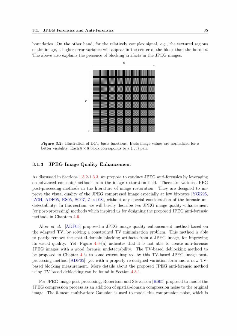
3.1. JPEG Forensics and Anti-Forensics 35
boundaries. On the other hand, for the relatively complex signal, e.g., the textured regionsof the image, a higher error variance will appear in the center of the block than the borders.The above also explains the presence of blocking artifacts in the JPEG images.
Figure 3.2: Illustration of DCT basis functions. Basis image values are normalized for abetter visibility. Each 8× 8 block corresponds to a (r, c) pair.
3.1.3 JPEG Image Quality Enhancement
As discussed in Sections 1.3.2-1.3.3, we propose to conduct JPEG anti-forensics by leveragingon advanced concepts/methods from the image restoration field. There are various JPEGpost-processing methods in the literature of image restoration. They are designed to im-prove the visual quality of the JPEG compressed image especially at low bit-rates [YGK95,LY04, ADF05, RS05, SC07, Zha+08], without any special consideration of the forensic un-detectability. In this section, we will briefly describe two JPEG image quality enhancement(or post-processing) methods which inspired us for designing the proposed JPEG anti-forensicmethods in Chapters 4-6.
Alter et al. [ADF05] proposed a JPEG image quality enhancement method based onthe adapted TV, by solving a constrained TV minimization problem. This method is ableto partly remove the spatial-domain blocking artifacts from a JPEG image, for improvingits visual quality. Yet, Figure 4.6-(a) indicates that it is not able to create anti-forensicJPEG images with a good forensic undetectability. The TV-based deblocking method tobe proposed in Chapter 4 is to some extent inspired by this TV-based JPEG image post-processing method [ADF05], yet with a properly re-designed variation form and a new TV-based blocking measurement. More details about the proposed JPEG anti-forensic methodusing TV-based deblocking can be found in Section 4.3.1.
For JPEG image post-processing, Robertson and Stevenson [RS05] proposed to model theJPEG compression process as an addition of spatial-domain compression noise to the originalimage. The 0-mean multivariate Gaussian is used to model this compression noise, which is

36 Chapter 3. Prior Art of JPEG and Median Filtering (Anti-)Forensics
treated as a random quantity. Moreover, the compression noise and the original image areassumed to be independent. With a proper image prior model, quality enhanced JPEG imagecan be obtained by using the MAP estimation. A more detailed description can be foundin Section 6.2.1. Moreover, a novel JPEG image quality enhancement method is proposed inSection 6.2.2, inspired by the JPEG compression noise model [RS05] and a sophisticated imageprior model [ZW11]. From Table 6.5, again we can see that JPEG image quality enhancementmethod does help to partly remove JPEG artifacts, yet not enough to reach a satisfactoryforensic undetectability level. Anti-forensic terms/strategies are to be proposed to fulfil thetask for further removing the remaining JPEG artifacts for anti-forensic considerations. Adetailed description of the proposed JPEG anti-forensic method supported by experimentalresults can be found in Sections 6.3-6.4.
3.1.4 Detecting JPEG Compression
Fan and De Queiroz [FD03] proposed an algorithm for maximum-likelihood estimation (MLE)of the JPEG quantization table, from a spatial-domain bitmap representation of the image.The method can also serve as a detector to classify an image as not JPEG compressed, ifeach entry of the estimated quantization table is either 1 or “undetermined” [FD03, Sta+10a,SL11].
Focusing on 8 × 8 block boundaries, Fan and De Queiroz [FD03] also proposed a JPEGblocking signature measure as:
KF =∑
k
|HI(k)−HII(k)| , (3.6)
where HI and HII are normalized histograms of pixel value differences across block boundariesand within the block, respectively (see [FD03] for details).
Luo et al. [LHQ10] proposed a scalar feature to distinguish JPEG images from uncom-pressed ones, based on the AC coefficient distribution change in the range of (−1, 1) and thatin the union range of (−2,−1] and [1, 2).
As to the quantization step estimation, Luo et al. [LHQ10] further estimated the ACcomponent quantization step as the integer, which is greater than 2 and gives the maximumvalue of the DCT histogram. Experimental results show that this JPEG image detectoroutperforms Fan and De Queiroz’s method [FD03].
3.1.5 Disguising JPEG Artifacts
In the DCT domain, subband (r, c) contains the (r, c)-th DCT coefficient from each DCT coef-ficient block. For the AC component, i.e., subband (r, c) 6= (1, 1), the Laplacian distribution isa popular choice [LG00] for modeling the distribution of unquantized DCT coefficients. For theDC component, i.e., subband (1, 1), there is no general model representing its distribution.

3.1. JPEG Forensics and Anti-Forensics 37
Nevertheless, its DCT quantization noise can be assumed to follow a uniform distribution[Sta+10a, SL11].
In order to disguise the DCT-domain quantization artifacts of a JPEG image, Stamm et
al. [Sta+10a, SL11] proposed to add a dithering signal to the dequantized DCT coefficientsQ−1(Q(DX)), so that the dithered DCT coefficients approximate the estimated distributionof the unquantized ones. This JPEG anti-forensic method succeeds in fooling the quantizationtable estimation based detector proposed in [FD03].
After the dithering operation, Stamm et al. [Sta+10b, SL11] later proposed an anti-forensicdeblocking operation against the blocking artifacts detector in [FD03], that is, the blockingsignature measure KF of Eq. (3.6). For a given image U, the anti-forensically deblocked imageU is obtained according to:
Ui,j = meds(Ui,j) + wi,j , (3.7)
where meds(·) is the median filtering operation with local window size s × s, and wi,j is alow-power white Gaussian noise of variance σ2.
Valenzise et al. proposed a perceptual anti-forensic dithering operation [VTT11], whoseresulting anti-forensic JPEG image has a higher perceptual quality than the one processedby Stamm et al.’s dithering method [Sta+10a, SL11]. A “just-noticeable distortion” (JND)[WN09] criterion is adopted to control the amount of introduced distortion. A minimum-costbipartite graph matching problem is used as the mathematical model for the adaptive insertionof the dithering signal. A greedy algorithm is implemented to get an approximate solution inorder to reduce the computation cost.
3.1.6 Attacking JPEG Anti-Forensics
Valenzise et al. [VTT11, Val+11, VTT13] claimed that the dithering signal of [Sta+10a] de-grades the image quality by introducing noise. Inspired by the JPEG ghosts detector [Far09b],they designed an efficient detector against JPEG anti-forensic dithering, which examines thenoisiness of re-compressed versions of the image under test. The TV of the re-compressedimage (the ℓ1 norm of the spatial first-order derivatives) [ROF92] is employed as the imagenoisiness measure. For a given image U, the detector re-compresses it using different qualityfactors q = 1, 2, . . . , 100, as a function of which, TV(q) is computed as the total variation ofthe re-compressed image. The first order backward finite difference ∆TV(q) is calculated as:
∆TV(q) = TV(q)− TV(q − 1), (3.8)
with TV(0) prescribed to be 0. The forensic measure is:
KV = maxq∈{1,2,··· ,100}
∆TV(q). (3.9)
Lai and Böhme [LB11] proposed another calibration-based detector to counter Stamm

38 Chapter 3. Prior Art of JPEG and Median Filtering (Anti-)Forensics
et al.’s JPEG anti-forensic method [Sta+10a, SL11], borrowing the idea of calibration fromsteganalysis [FGH02]. The detector compares the variances of the corresponding subbandsfrom a given image U and its calibrated version Ucal, which is obtained by cropping U by 4
pixels both horizontally and vertically. The calibrated feature KL is then established as:
KL =1
28
28∑
k=1
∣
∣
∣
∣
var(DkU)− var(DkUcal)
var(DkU)
∣
∣
∣
∣
, (3.10)
where var(·) returns the sample variance of the input vector, and Dk is a matrix extractingthe DCT coefficients of the k-th high-frequency subband (as defined in [LB11]).
3.1.7 Other Relevant Methods
Moreover, some relative techniques can also be extended for JPEG anti-forensics, e.g., theShrink-and-Zoom (SAZ) attack proposed by Sutthiwan and Shi [SS11], though it was initiallydesigned for double JPEG anti-forensics. Given a JPEG image, a shrinkage (image down-scaling) operation is firstly applied; then the processed image is zoomed back to the same sizeas the original one, to obtain the anti-forensic JPEG image.
Li et al. [LLH12] considered the process of creating anti-forensic JPEG image [Sta+10a,Sta+10b, SL11] as data hiding, in the view of JPEG steganalysis. The anti-forensic processchanges the intra- and inter-block statistics of the image, which can be measured using a groupof Markov process transition probability matrices [CS08]. A 100-dimensional feature vectoris then extracted and fed to an SVM for building the JPEG forensic detector. Similarly, thewell-known Subtractive Pixel Adjacency Matrix (SPAM) feature vector [PBF10] has also beenused for countering JPEG anti-forensics [VTT13].
3.1.8 Summary
In this thesis, the JPEG forensic detectors described in Sections 3.1.4, 3.1.6, and 3.1.7 areused for forensic testing for different (anti-forensic) JPEG images. For the sake of conciseness,we hereafter use symbols for referring to the detectors, which are summarized in Table 3.1.Here, we mainly name the detectors directly after the feature value name, e.g., KF , KV , andKL in Eqs. (3.6), (3.9), and (3.10), respectively. The subscript of the detector name is basedon the surname of the first author of the corresponding algorithm. We use the superscript‘S’ together with the dimensionality of the feature vector to indicate that KS100
Li and KS686P
are SVM-based detectors. Meanwhile, the superscript ‘Q’ of KQF and KQ
Luo shows that theyestimate quantization steps. Note that Kp
U (parameters p = 1, and p = 2 are consideredhere) is a new family of JPEG blocking detectors proposed in this thesis (see Eq. (4.3) inSection 4.2.2).
Practically, in some high-frequency subbands of highly JPEG compressed images, all theDCT coefficients are quantized to 0 and no quantization step could be determined. Hence,

3.1. JPEG Forensics and Anti-Forensics 39
Table 3.1: JPEG forensic detectors.
KQF Fan and De Queiroz’s [FD03] quantization table estimation based
detector;
KF Fan and De Queiroz’s [FD03] JPEG blocking artifacts detector;
KLuo Luo et al.’s [LHQ10] JPEG identifying detector;
KQLuo Luo et al.’s [LHQ10] quantization step estimation based detector;
KV Valenzise et al.’s [Val+11, VTT13] TV-based JPEG anti-forensicdetector;
KL Lai and Böhme’s [LB11] calibration-based detector;
K1U ,K
2U the proposed JPEG blocking artifacts detectors (see Eq. (4.3));
KS100Li Li et al.’s [LLH12] 100-dimensional intra- and inter-block
correlation feature [CS08] based detector;
KS686P Pevný et al.’s [PBF10] 686-dimensional SPAM feature based
detector.
for detector KQLuo, we use the number of defined estimated quantization steps greater than
1 as the final feature value. Besides, the range of the re-compression quality factor q inEq. (3.9) is shrunk to {45, 46, · · · , 100}, as we use the JPEG images compressed with qualityfactors randomly selected from {50, 51, · · · , 95} in this thesis. Though detector KQ
F is analyzedas not very reliable in Section 4.2.1, as it may result in relatively high false positive rate(detecting never compressed images as anti-forensic JPEG images), we still test it. Followingthe suggestion in [FD03, Sta+10a, SL11], a given image is classified as never compressed ifand only if its estimated quantization table is full of entries 1 or “undetermined”. We willreport the rate of correctly detecting anti-forensic JPEG images for detector KQ
F .
Table 3.2 briefly reviews the state-of-the-art anti-forensic JPEG images, which will be usedfor comparison with the anti-forensic JPEG images processed using the proposed methods inChapters 4-6. In order to create this state-of-the-art anti-forensic JPEG image FJ
SqSb[Sta+10a,
Sta+10b, SL11], we set s = 3 and σ2 = 2 (see Section 3.1.5 and Eq. (3.7)), following thesetting in the original papers. Also for the sake of brevity, we hereafter use the symbols listedin Table 3.2 for referring to the original, JPEG, or state-of-the-art anti-forensic JPEG images.
From Sections 3.1.5 and 3.1.7, we can see that the state-of-the-art JPEG anti-forensicmethods use noise injection [Sta+10a, SL11, VTT11] or simple image processing operations(e.g., median filtering [Sta+10b, SL11], and resampling [SS11]), in order to remove telltaleartifacts from a JPEG image. These operations may be effective for removing the DCT-domain quantization artifacts or the spatial-domain blocking artifacts. However, they alsolargely degrade the visual quality of the processed image [VTT11, Val+11, VTT13], whichcan still detected by other advanced JPEG forensic detectors [Val+11, LB11, VTT13].
In Chapters 4-6, we follow another research line for JPEG anti-forensics, by adopting someconcepts/methods from JPEG image restoration field. We hope to created anti-forensic JPEGimages with a better forensic undetectability against the detectors listed in Table 3.1 as well

40 Chapter 3. Prior Art of JPEG and Median Filtering (Anti-)Forensics
Table 3.2: Notations for original, JPEG, and state-of-the-art anti-forensic JPEG images.
I genuine, uncompressed image;
J JPEG image;
FJSq
Stamm et al.’s [Sta+10a, SL11] anti-forensic JPEG image createdfrom J using the dithering operation (see Section 3.1.5);
FJSqSb
Stamm et al.’s [Sta+10b, SL11] anti-forensic JPEG image createdfrom FJ
Squsing the median filtering based method (see Section 3.1.5);
FJV Valenzise et al.’s [VTT11] anti-forensic JPEG image created from J
using the perceptual anti-forensic dithering operation (seeSection 3.1.5);
FJSu Sutthiwan and Shi’s [SS11] anti-forensic JPEG image created from
J using the SAZ attack (see Section 3.1.7).
as a higher visual quality of the anti-forensic JPEG image, compared with the state-of-the-artanti-forensic JPEG images listed in Table 3.2.
3.2 Median Filtering Forensics and Anti-Forensics
3.2.1 Median Filtering Basics and Artifacts
Let x = (x1,x2, · · · ,xi, · · · ,xN )T denote the given original grayscale image (in vectorizedform) of N pixels, the i-th pixel of its median filtered version can be obtained by:
yi = median (Pix), (3.11)
where Pi is an s2×N sparse matrix extracting the i-th overlapping image block of size s×s (sis an odd number), and xi locates in the geometrical center of block Pix. Note that median(·)returns the median value of the input sample vector. Different windows can be used for imagemedian filtering [PV92]. In this thesis, we only consider the square window, which probablyis the most commonly used one. We use the notation MF (m)(·) for the image processingoperation, which applies median filtering to the input for m (> 0) time(s).
Without loss of generality, in this thesis, we perform median filtering anti-forensics onimages which have been median filtered once, with s = 3. It is also the experimental settingin all the state-of-the-art median filtering anti-forensic methods [FB12, WSL13, DN+13]. Forthe sake of brevity, we hereafter use the abbreviation “MF image” to refer to the “medianfiltered” image.
Within a certain neighborhood of the MF image, the probability of pixel values originatefrom the same pixel of the original image is high. This effect is called “streaking” by Bovik[Bov87]. The streaking artifacts can also be inferred from the shape change of the pixel
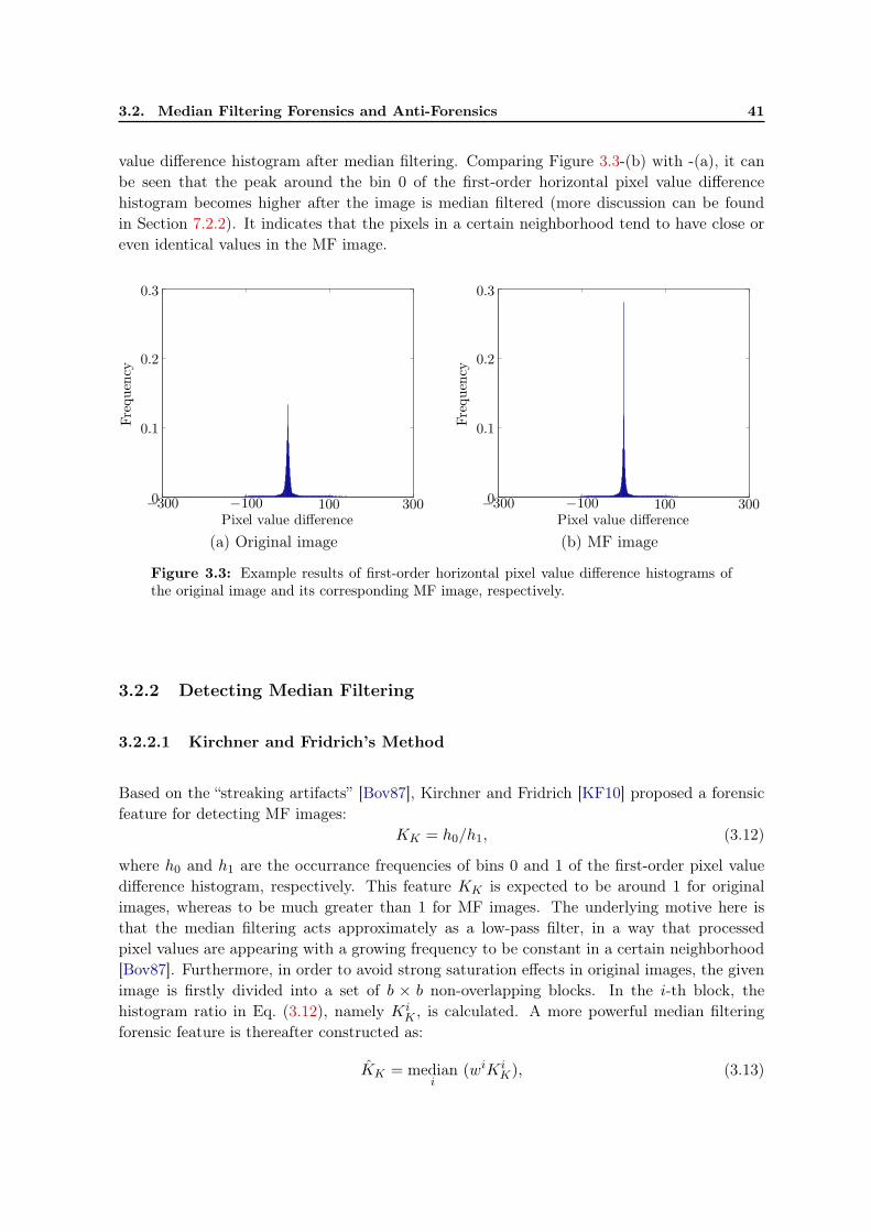
3.2. Median Filtering Forensics and Anti-Forensics 41
value difference histogram after median filtering. Comparing Figure 3.3-(b) with -(a), it canbe seen that the peak around the bin 0 of the first-order horizontal pixel value differencehistogram becomes higher after the image is median filtered (more discussion can be foundin Section 7.2.2). It indicates that the pixels in a certain neighborhood tend to have close oreven identical values in the MF image.
Pixel value difference
Frequency
−300 −100 100 3000
0.1
0.2
0.3
(a) Original image
Pixel value difference
Frequency
−300 −100 100 3000
0.1
0.2
0.3
(b) MF image
Figure 3.3: Example results of first-order horizontal pixel value difference histograms ofthe original image and its corresponding MF image, respectively.
3.2.2 Detecting Median Filtering
3.2.2.1 Kirchner and Fridrich’s Method
Based on the “streaking artifacts” [Bov87], Kirchner and Fridrich [KF10] proposed a forensicfeature for detecting MF images:
KK = h0/h1, (3.12)
where h0 and h1 are the occurrance frequencies of bins 0 and 1 of the first-order pixel valuedifference histogram, respectively. This feature KK is expected to be around 1 for originalimages, whereas to be much greater than 1 for MF images. The underlying motive here isthat the median filtering acts approximately as a low-pass filter, in a way that processedpixel values are appearing with a growing frequency to be constant in a certain neighborhood[Bov87]. Furthermore, in order to avoid strong saturation effects in original images, the givenimage is firstly divided into a set of b × b non-overlapping blocks. In the i-th block, thehistogram ratio in Eq. (3.12), namely Ki
K , is calculated. A more powerful median filteringforensic feature is thereafter constructed as:
KK = mediani
(wiKiK), (3.13)
42 Chapter 3. Prior Art of JPEG and Median Filtering (Anti-)Forensics
where wi = 1−(
hi0
b2−b
)
is the weight function. Note that hi0 is the occurrence frequency of bin
0 for the first-order pixel value difference histogram in the i-th block. In [KF10], it is suggestedto set b = 64, for a good tradeoff between the forensic detectability and computation cost ofthe feature.
By adopting the SVM, Kirchner and Fridrich [KF10] also showed the effectiveness of usingthe well-known SPAM feature vector [PBF10] to discriminate MF images from the originalimages.
3.2.2.2 Cao et al.’s Method
After an original image is median filtered, the probability of zero values in the first-order pixelvalue difference map increases, especially in textured regions. Based on this analysis, Cao et
al. [Cao+10] proposed another median filtering forensic feature:
KC =
∑
i(∆ru)i · vi√
2∑
i vi
+
∑
i(∆cu)i · vi√
2∑
i vi
, (3.14)
where (∆ru)i (or (∆cu)i) is 1 if the i-th element in the first-order row (or column) pixel valuedifference map is zero, or is 0 otherwise; and v is the binary local variance map, indicatingtextured regions (vi = 1) or smooth regions (vi = 0) of the image (see [Cao+10] for moredetails).
3.2.2.3 Yuan’s Method
Median filtering is based on order-statistics. Therefore, it affects the order and the pixel valuelevel inside the image block Piu. Besides, the median filter works on overlapping blocks,which leads to the appearance of certain dependency artifacts. In order to capture theselocal dependency artifacts, Yuan [Yua11] proposed 5 feature vectors: fDBM , fOBC , fQGL,fDBC , and fFBC (see [Yua11] for details), which are together recognized as the MFF (MedianFiltering Forensics) feature vector fMFF . The median filtering forensic detector is thereafterbuilt with the adoption of the SVM. Moreover, the above 5 feature vectors can be furthermerged as a single scalar feature:
KY =fDBM5 fOBC
2 fQGL6
(
fDBC3 + fDBC
7 − fDBC2 − fDBC
6
)
fFBC3
fOBC1 f
QGL9
(
fDBC2 + fDBC
8 − fDBC1 − fDBC
9
)
fFBC2 fFBC
9
. (3.15)
Experimental results show that the merged discriminating feature also performs excellently,though the MFF feature is more powerful.

3.2. Median Filtering Forensics and Anti-Forensics 43
3.2.2.4 Chen et al.’s Method
It is obvious that the overlapping median filter windows lead to certain correlations in aneighborhood of the MF image. Moreover, the median filter is based on order statistics,and is known to have good edge preserving capability. This makes the median filtered pixelneighbors correlate in a different way compared to those of the original or average filteredimages. For median filtering detection, Chen and Ni [CN11] proposed the EBPM (EdgeBased Prediction Matrix) feature to examine the statistical change among edge regions of theimage. The given image is firstly divided into non-overlapping blocks, which are classified tothree types. For each type of blocks, a neighborhood prediction model is employed, and theestimated prediction coefficients constitute the discriminating feature vector.
Chen et al. [Che+12, CNH13] further proposed a more powerful median filtering detectionfeature based on the analysis of statistical characterization in the pixel value difference domain.The proposed Global and Local Feature (GLF) vector fGLF consists of two sub-vectors: theglobal probability feature vector fGPF , and the local correlation feature vector fLCF . Theconstruction of fGPF is based on the observation that the empirical cumulative distributionin the pixel value difference domain differs considerably among different types of images, e.g.,original, median filtered, and average filtered images. The motivation to build fLCF is that theMF image has a rather distinct intrinsic fingerprint for the adjacent difference pair correlationin the pixel value difference domain.
3.2.2.5 Kang et al.’s Method
Kang et al. [PK12, Kan+12, Kan+13] proposed to use the median filter residual of a givenimage u (input of the forensic detector) to distinguish MF images from other kinds of images:
r =MF (1)(u)− u. (3.16)
In [PK12], Peng and Kang used the second-order Markov process [PBF10] to model the me-dian filtered residual. The MFRTP (Median Filter Residual Transition Probabilities) featurevector is thereafter extracted and fed to the SVM for building the median filtering detec-tor. Later, Kang et al. [Kan+12, Kan+13] adopted the autoregressive model to analyze themedian filter residual, and the coefficients are extracted as the MFRAR (Median Filter Resid-ual AutoRegressive) feature vector, which has a low dimensionality but still performs verywell. Their methods also achieve good robustness of median filtering detection against JPEGcompression post-processing.
3.2.2.6 Zhang et al.’s Method
Zhang et al. [Zha+14] investigated the median filtering from the angle of micro-texture struc-ture, with the adoption of the so-called local ternary pattern [TT10] and local derivative

44 Chapter 3. Prior Art of JPEG and Median Filtering (Anti-)Forensics
pattern [Zha+10]. In order to speed up the SVM training procedure, the dimensionality ofthe extracted MFLTP (Median Filter Local Ternary Patterns) feature is reduced from 2048to 220 using the kernel principal component analysis technique, without harming the forensicperformance of the detector.
3.2.3 Disguising Median Filtering Artifacts
3.2.3.1 Fontani and Barni’s Method
Fontani and Barni [FB12] pioneered the median filtering anti-forensic work, against the forensicdetectors proposed in [KF10, Cao+10, Yua11] (see Sections 3.2.2.1-3.2.2.3). The main idea oftheir method is to find a proper convolution filter f , so that the filtered MF image f(y) haslow detector output while still close to y. The searching of f is performed by minimizing thefollowing cost function:
f = arg minf
(exp (KY (f (y))− 2.2)− PSNR (y, f (y))) , (3.17)
whereKY (·) (see Eq. (3.15)) returns the value of Yuan’s merged discriminating feature [Yua11]for the input image, and the definition of PSNR(·, ·) can be found in Section 2.2.2.1. The finalanti-forensic MF image is generated by convolution filtering: x = f(y).
3.2.3.2 Wu et al.’s Method
Wu et al. [WSL13] modeled the pixel value difference pair di,j(u) = [Ui,j − Ui,j+1,Ui,j −Ui+1,j ]
T , using a 2-dimensional generalized Gaussian distribution. Targeting at median fil-tering forensic detectors in [KF10, PBF10, Yua11] (see Sections 3.2.2.1 and 3.2.2.3), a noiseattack algorithm is thereafter proposed for median filtering anti-forensic purposes:
di,j(x) = di,j(y) + ni,j , (3.18)
where n is the attacking noise. The goal is to bring the distribution of di,j(x) close to theestimated one of the original image pixel value difference di,j(x). The distribution of ni,j
is obtained based on the following two assumptions: the convolution of the distributions ofdi,j(y) and ni,j yields the distribution of di,j(x); and the parameters of the two distributionsof di,j(y) and di,j(x) have linear correlations.
3.2.3.3 Dang-Nguyen et al.’s Method
Dang-Nguyen et al. [DN+13] proposed another noise attack to the MF image, targeting atforensic detectors in [KF10, Cao+10, Yua11] (see Sections 3.2.2.1-3.2.2.3). The given image isfirstly divided into non-overlapping blocks. The major noise attack is performed in relativelycomplex blocks, whose variances are greater than a certain threshold T . If the complex block

3.2. Median Filtering Forensics and Anti-Forensics 45
does not contribute to Yuan’s fDBM and fOBC features [Yua11], the block is then ditheredwith random noise uniformly distributed in [−7,−3] ∪ [3, 7]. At last, the whole image isattacked by random noise uniformly distributed in [0, 1].
3.2.4 Summary
For the sake of conciseness, we henceforth use symbols for referring to the detectors consideredin our work on median filtering anti-forensics, which are summarized in Table 3.3. Similar toTable 3.1, we mainly name the detectors directly after the feature value name for the scalar-based median filtering forensic detectors. As to the SVM-based detectors, the superscript ‘S’together with the dimensionality of the feature vector is used to indicate that they are SVM-based. Note that, if the same (group of) authors have contributed more than one SVM-baseddetectors, we choose the latest (also the strongest) one for forensic testing.
Table 3.3: Median filtering forensic detectors.
KK Kirchner and Fridrich’s [KF10] first-order pixel value differencehistogram based detector;
KK the block-based version of detector KK [KF10];
KC Cao et al.’s [Cao+10] first-order pixel value difference based detector;
KY Yuan’s [Yua11] merged discriminating feature based detector;
KS686SPAM the 686-dimensional SPAM feature based detector [PBF10];
KS44MFF Yuan’s [Yua11] 44-dimensional MFF feature based detector;
KS56GLF Chen et al.’s [Che+12, CNH13] 56-dimensional GLF feature based
detector;
KS10AR Kang et al.’s [Kan+12, Kan+13] 10-dimensional MFRAR feature
based detector;
KS220LTP Zhang et al.’s [Zha+14] 220-dimensional MFLTP feature based
detector.
From Section 3.2.3, we can see that the state-of-the-art median filtering anti-forensic meth-ods use image processing operations (e.g., convolution filtering [FB12]), or noise injection[WSL13, DN+13], in order to remove telltale artifacts from an MF image. The resultinganti-forensic MF image not necessarily achieves a good forensic undetectability against theforensic detectors listed in Table 3.3, and normally suffers from low visual quality.
In Chapter 7, we follow another research line for median filtering anti-forensics, leveragingon image deconvolution. We hope to create anti-forensic MF images with a better forensicundetectability against the detectors listed in Table 3.3 as well as a higher visual quality ofthe anti-forensic MF image, compared with the state-of-the-art anti-forensic MF images listedin Table 3.411.
11In [DN+13], Dang-Nguyen et al. show that their median filtering anti-forensic method outperforms Fontaniand Barni’s [FB12]. In Chapter 7, we refrain from comparing with Fontani and Barni’s pioneer anti-forensicMF image [FB12], which is therefore not included in Table 3.4.

46 Chapter 3. Prior Art of JPEG and Median Filtering (Anti-)Forensics
Table 3.4: Notations for original, MF, and state-of-the-art anti-forensic MF images.
I original, intact image;
M MF image;
FMW Wu et al.’s [Sta+10b, SL11] anti-forensic MF image created fromM using
the dithering operation (see Section 3.2.3.2);
FMD Dang-Nguyen et al.’s [DN+13] anti-forensic MF image created from M
using the noise injection based method (see Section 3.2.3.3).

Chapter 4
Total Variation Based JPEG
Anti-Forensics
Contents4.1 Introduction and Motivation . . . . . . . . . . . . . . . . . . . . . . . . . 48
4.2 Performance Analysis of Scalar-Based JPEG Detectors . . . . . . . . 49
4.2.1 Quantization Table Estimation Based Detector . . . . . . . . . . . . . . . 49
4.2.2 Other Scalar-Based JPEG Forensic Detectors . . . . . . . . . . . . . . . . 51
4.3 JPEG Anti-Forensics via TV-Based Deblocking . . . . . . . . . . . . . 53
4.3.1 JPEG Deblocking Using Constrained TV-Based Minimization . . . . . . . 53
4.3.2 De-Calibration . . . . . . . . . . . . . . . . . . . . . . . . . . . . . . . . . 56
4.4 Experimental Results . . . . . . . . . . . . . . . . . . . . . . . . . . . . . 56
4.4.1 Parameter Settings . . . . . . . . . . . . . . . . . . . . . . . . . . . . . . . 56
4.4.2 Comparison and Analysis . . . . . . . . . . . . . . . . . . . . . . . . . . . 58
4.5 Summary . . . . . . . . . . . . . . . . . . . . . . . . . . . . . . . . . . . . 61
In this chapter, we focus on removing the JPEG blocking artifacts at the anti-forensiclevel. To this end, we propose a constrained TV-based minimization problem, whose cost
function consists of a TV term and a TV-based blocking measurement term. The resultinganti-forensic JPEG image successfully fools the forensic methods detecting JPEG blocking,and other advanced JPEG forensic detectors. The calibration-based detector is also defeatedby conducting a further feature value minimization. Experimental results show that theproposed method outperforms the state-of-the-art JPEG anti-forensic methods in a betterforensic undetectability and a higher visual quality of the processed image.
A paper describing the proposed method was published in an international conference[Fan+13a]. The Matlab code of the method is freely shared online and can be down-loaded from: http://www.gipsa-lab.grenoble-inp.fr/~wei.fan/documents/TV-AFJPG-
ICASSP13.tar.gz.
47

48 Chapter 4. Total Variation Based JPEG Anti-Forensics
4.1 Introduction and Motivation
For JPEG anti-forensic purposes, we need to consider both the quantization artifacts in theDCT domain and the blocking artifacts in the spatial domain. In practice, we find it extremelydifficult to conduct a single-step attack to defeat multiple JPEG forensic detectors that workin different domains, while keeping a high image visual quality. Therefore, in this thesis, weconsider removing JPEG artifacts alternatively in the spatial and in the DCT domains. Asimilar strategy is adopted in Stamm et al.’s JPEG anti-forensic method [Sta+10a, Sta+10b,SL11], where the DCT-domain quantization artifacts and the spatial-domain blocking artifactsare handled separately in different domains.
For JPEG post-processing in image restoration, the quantization artifacts in the DCTdomain is not the main concern. Its main objective is to remove the spatial-domain JPEGblocking artifacts for visual quality enhancement purposes [LY04, ADF05, Zha+08]. Unfor-tunately, these JPEG deblocking methods may not be able to create post-processed JPEGimages which are able to pass the examination of JPEG blocking detectors. However, byintegrating some additional anti-forensic terms, these methods can contribute in the JPEGblocking artifacts removing task at the anti-forensic level. Based on the above analysis, herewe choose to firstly focus on the spatial-domain JPEG blocking artifacts. We leave the taskof DCT-domain quantization artifacts removing in Chapter 5. Following the research line ofconducting image anti-forensics leveraging on image restoration, in this chapter, we devise aJPEG anti-forensic method based on TV regularization.
The concept of Total Variation (i.e., TV for short) regularization was pioneered by Rudinet al. [ROF92] in 1992. Ever since then, it has been widely used in image restoration, forvarious applications such as denoising, deconvolution, inpainting, etc. Take denoising as anexample, the integral of the absolute gradient of the noised signal is high, in other words, thenoised signal has high TV. Therefore, the signal restoration can be conducted by reducing theTV of the noised signal, usually with a signal fidelity constraint with respect to the noisedsignal. Compared with traditional techniques, e.g., linear smoothing, and median filtering, theTV-based denoising is not only simple and effective in noise removal but also able to preservedetails such as edges.
For JPEG image, the blocking artifacts in the spatial domain are presented in the formof pixel value discontinuities around the 8 × 8 block borders. This kind of artifacts leads tohigh TV of the JPEG image. Therefore, JPEG deblocking can be performed by minimizinga TV-based energy function [ADF05]. Traditionally, its main objective is to improve the vi-sual quality of the JPEG image. In this chapter, we add another TV-based JPEG blockingmeasurement term into the TV-based minimization cost function. By solving the new mini-mization problem, we may need to sacrifice some image quality of the JPEG image. However,we hope to create anti-forensic JPEG images which are able to fool existing scalar-based JPEGforensic detectors.
The remainder of this chapter is organized as follows. Section 4.2 experimentally analyzesthe forensic performance of 8 existing scalar-based JPEG forensic detectors listed in Table 3.1.

4.2. Performance Analysis of Scalar-Based JPEG Detectors 49
In Section 4.3, we describe the proposed TV-based deblocking method for JPEG anti-forensics.Experimental results with comparisons with state-of-the-art JPEG anti-forensic methods arepresented in Section 4.4. At last, Section 4.5 summarizes this chapter.
4.2 Performance Analysis of Scalar-Based JPEG Detectors
In this section, we experimentally analyze the performance of the 8 scalar-based JPEG de-tectors. As to the other 2 SVM-based JPEG detectors listed in Table 3.1, we leave it to bediscussed in Chapter 5.
4.2.1 Quantization Table Estimation Based Detector
Fan and De Queiroz’s [FD03] JPEG forensic detector KQF (see Section 3.1.4 and Table 3.1)
classifies a given image as not compressed, if all the estimated quantization steps are either 1
or “undetermined” [Sta+10a]. It is the targeted quantization artifacts detector of the JPEGanti-forensic method proposed in [SL11]. However, as pointed out by Böhme and Kirchner[BK13], we lack knowledge on the false positive rate of KQ
F [FD03].
In order to investigate the reliability of KQF [FD03], we estimated the quantization table of
10, 000 genuine, uncompressed 512× 512 PGM images from BOSSBase dataset [BFP11] (seethe end of Section 2.3.1 for more descriptions and discussions concerning this dataset). Table4.1 lists the false positive rate PFP of all the 10 archives of BOSSBase. Surprisingly, PFP canreach as high as 61.50% for the 6-th archive. The average rate 25.22% also indicates that KQ
F
is not very reliable to determine whether an image has been JPEG compressed.
Furthermore, we found that among all the “non-1” and “non-undetermined” estimatedentries by KQ
F [FD03], 3 takes a large portion, as shown in the P3 column in Table 4.1.Figure 4.1-(a) is an example DCT histogram from a never compressed image, which has nocomb-like quantization artifacts but is detected as quantized by 3 according to KQ
F . Here wego back to review the MLE of quantization table [FD03]. For the sake of simplicity, we onlyanalyze why KQ
F picks 3 instead of 1 in this case. Based on the Eq. (14) of [FD00] and theEq. (15) of [FD03], for quantization step q = 1, the log-likelihood is:
L(1) = N × w(0, 1) +N × log 1, (4.1)
while the log-likelihood for q = 3 is:
L(3) = p0 ×N × w(0, 3) + (1− p0)×N × w(1, 3) +N × log 3, (4.2)
where N is the total number of blocks used in estimation, and w(i, q) is an even functionof i defined in [FD00] (more details can be found in [FD00, FD03]). We denote p0 as thepercentage of coefficients which are the integer multiples of 3. KQ
F chooses 3 instead of 1

50 Chapter 4. Total Variation Based JPEG Anti-Forensics
Table 4.1: PFP and P3 for detector KQF [FD03] on BOSSBase dataset [BFP11]. PFP is
calculated as the portion of images which are mistakenly classified as JPEG compressedamong all the original images under examination. P3 is the fraction of the number ofestimated quantization steps being 3 over the number of the estimated “non-1” and “non-undetermined” quantization steps.
Archive PFP (%) P3
01 18.70 1653/1959 = 84.38%
02 12.40 957/1118 = 85.60%
03 4.50 175/187 = 93.58%
04 5.70 111/125 = 88.80%
05 10.50 986/1141 = 86.42%
06 61.50 9243/11033 = 83.78%
07 17.50 1084/1155 = 93.85%
08 43.90 5655/6670 = 84.78%
09 33.20 5062/5895 = 85.87%
10 44.30 6780/7720 = 87.82%
Average 25.22 87.49%
when L(3) > L(1). This happens when p0 > 67.28%. For Figure 4.1-(a), among all 408312
DCT coefficients in use for quantization step estimation, there are 2797 coefficients which areinteger multiples of 3, namely p0 = 68.50%. Hence KQ
F detects that it is quantized by 3. Thisfrequently happens in the high-frequency subbands for relatively smooth images.
Another interesting point is that KQF outputs 1 for some DCT histograms which are obvi-
ously not from genuine, uncompressed images. Figure 4.1-(b) is from a post-processed JPEGimage. It is obvious that the comb-like quantization artifacts still remain, but KQ
F fails toestimate the correct quantization step.
When KQF is tested on UCIDTest dataset (see Section 2.3.1 for more details concerning this
dataset) with 1000 UCID images [SS04]. The false positive rate is PFP = 16/1000 = 1.6%,and P3 = 15/16 = 94.74%. This low false positive rate is due to the fact that most UCIDimages contain a large portion of highly textured regions, which decreases the occurrences of 3in the quantization step estimation. Nevertheless the weakness of KQ
F is exposed when testedon the dataset BOSSBase where images are relatively smooth (also see the discussion in theend of Section 2.3.1).
From the above analysis of detector KQF , it can be seen that it is not a very reliable forensic
detector to determine whether an image has been previously JPEG compressed. However, inour JPEG anti-forensic work, we still consider the outputs of KQ
F trying to decrease the
12For an image with size of 512× 512, there should be 4096 DCT coefficients in each subband. However, forestimating the quantization step [FD03], the 8×8 block with equal value for all the 64 pixels is excluded in theMLE. Therefore, here in this example DCT histogram, there are only 4083 instead of 4096 DCT coefficientsused in the estimation.
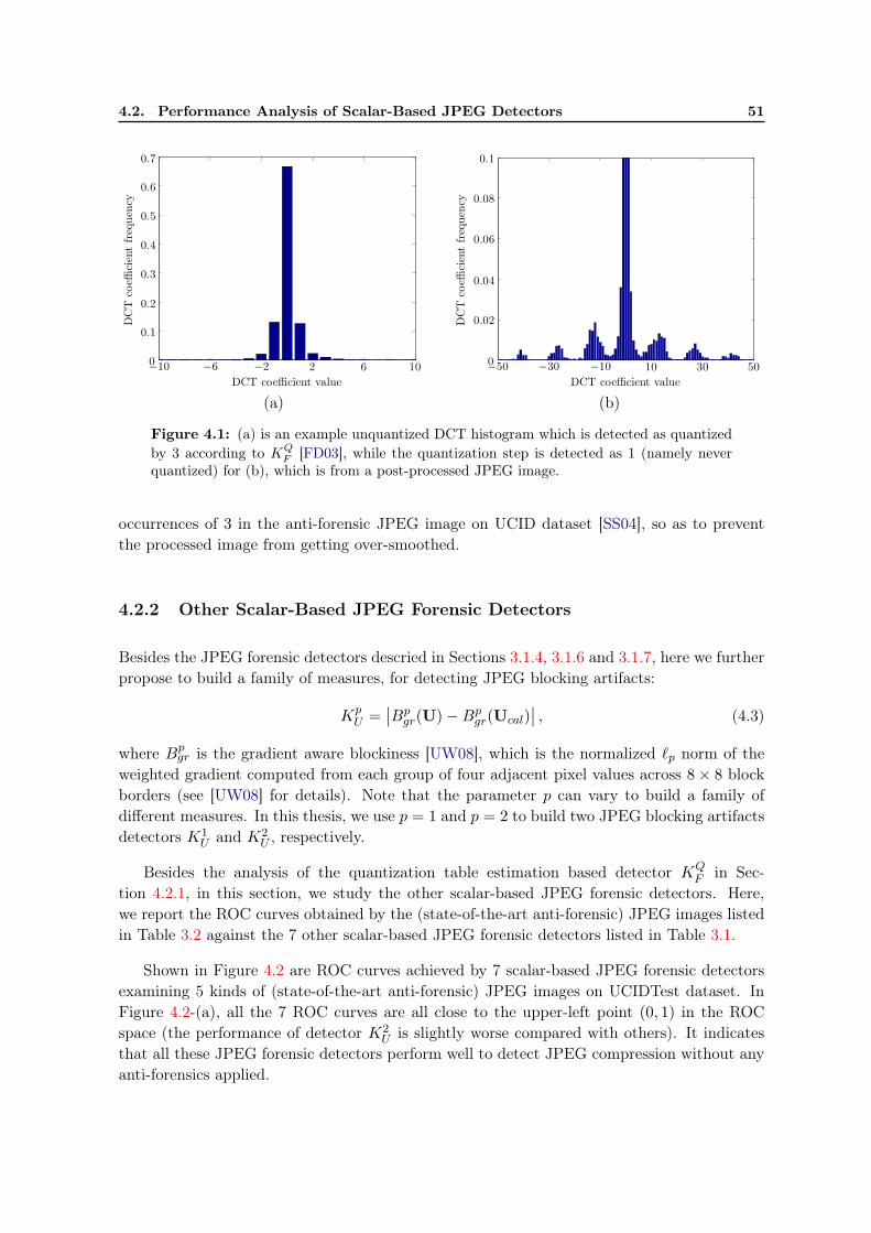
4.2. Performance Analysis of Scalar-Based JPEG Detectors 51
DCT coefficient value
DCT
coeffi
cientfrequen
cy
−10 −6 −2 2 6 100
0.1
0.2
0.3
0.4
0.5
0.6
0.7
(a)DCT coefficient value
DCT
coeffi
cientfrequen
cy
−50 −30 −10 10 30 500
0.02
0.04
0.06
0.08
0.1
(b)
Figure 4.1: (a) is an example unquantized DCT histogram which is detected as quantized
by 3 according to KQF [FD03], while the quantization step is detected as 1 (namely never
quantized) for (b), which is from a post-processed JPEG image.
occurrences of 3 in the anti-forensic JPEG image on UCID dataset [SS04], so as to preventthe processed image from getting over-smoothed.
4.2.2 Other Scalar-Based JPEG Forensic Detectors
Besides the JPEG forensic detectors descried in Sections 3.1.4, 3.1.6 and 3.1.7, here we furtherpropose to build a family of measures, for detecting JPEG blocking artifacts:
KpU =
∣
∣Bpgr(U)−Bp
gr(Ucal)∣
∣ , (4.3)
where Bpgr is the gradient aware blockiness [UW08], which is the normalized ℓp norm of the
weighted gradient computed from each group of four adjacent pixel values across 8× 8 blockborders (see [UW08] for details). Note that the parameter p can vary to build a family ofdifferent measures. In this thesis, we use p = 1 and p = 2 to build two JPEG blocking artifactsdetectors K1
U and K2U , respectively.
Besides the analysis of the quantization table estimation based detector KQF in Sec-
tion 4.2.1, in this section, we study the other scalar-based JPEG forensic detectors. Here,we report the ROC curves obtained by the (state-of-the-art anti-forensic) JPEG images listedin Table 3.2 against the 7 other scalar-based JPEG forensic detectors listed in Table 3.1.
Shown in Figure 4.2 are ROC curves achieved by 7 scalar-based JPEG forensic detectorsexamining 5 kinds of (state-of-the-art anti-forensic) JPEG images on UCIDTest dataset. InFigure 4.2-(a), all the 7 ROC curves are all close to the upper-left point (0, 1) in the ROCspace (the performance of detector K2
U is slightly worse compared with others). It indicatesthat all these JPEG forensic detectors perform well to detect JPEG compression without anyanti-forensics applied.

52 Chapter 4. Total Variation Based JPEG Anti-Forensics
False positive rate
Truepositiverate
0 0.2 0.4 0.6 0.8 10
0.2
0.4
0.6
0.8
1
KF
KLuo
KQLuo
KV
KL
K1U
K2U
Random guess
(a) J
False positive rate
Truepositiverate
0 0.2 0.4 0.6 0.8 10
0.2
0.4
0.6
0.8
1
KF
KLuo
KQLuo
KV
KL
K1U
K2U
Random guess
(b) FJSq
[Sta+10a, SL11]
False positive rate
Truepositiverate
0 0.2 0.4 0.6 0.8 10
0.2
0.4
0.6
0.8
1
KF
KLuo
KQLuo
KV
KL
K1U
K2U
Random guess
(c) FJSqSb
[Sta+10b, SL11]
False positive rate
Truepositiverate
0 0.2 0.4 0.6 0.8 10
0.2
0.4
0.6
0.8
1
KF
KLuo
KQLuo
KV
KL
K1U
K2U
Random guess
(d) FJV [VTT11]
False positive rate
Truepositiverate
0 0.2 0.4 0.6 0.8 10
0.2
0.4
0.6
0.8
1
KF
KLuo
KQLuo
KV
KL
K1U
K2U
Random guess
(e) FJSu [SS11]
Figure 4.2: ROC curves achieved by 5 kinds of (state-of-the-art anti-forensic) JPEG imagesagainst 7 scalar-based JPEG forensic detectors. Results are obtained on UCIDTest dataset.

4.3. JPEG Anti-Forensics via TV-Based Deblocking 53
Detectors KV [Val+11, VTT13] and KL [LB11] are proposed aiming at detecting the anti-forensic JPEG image FJ
Sq[Sta+10a, SL11]. Therefore, from Figure 4.2-(b), we can see that
both the two ROC curves respectively achieved by KV and KL are close to the upper-leftpoint of the ROC space, which implies a good forensic detectability. Valensize et al. [VTT11]improved the dithering based anti-forensic method of Stamm et al. [Sta+10a, SL11], byemploying the JND criterion to control the distortion introduced by the anti-forensic ditheringoperation. The resulting anti-forensic JPEG image FJ
V [VTT11] is able to achieve higher visualquality (see Table 4.2 for relevant quality comparison) but about the same level of forensicundetectability, compared with FJ
Sq[Sta+10a, SL11].
The anti-forensic JPEG image FJSqSb
[Sta+10b, SL11] is obtained by processing FJSq
[Sta+10a, SL11] using median filtering combined with white Gaussian noise addition. TheROC curves in Figure 4.2-(c) show that median filtering performs very well in disguisingJPEG blocking artifacts, against detectors KF [FD03], K1
U and K2U . Compared with other
state-of-the-art anti-forensic JPEG images, FJSqSb
[Sta+10b, SL11] is able to drag the ROCcurves the closest to the random guess. However, the ROC curves achieved by KLuo [LHQ10]and KV [Val+11, VTT13] are still quite far away from the random guess. Moreover, Böhmeand Kirchner [BK13] point out that FJ
SqSb[Sta+10b, SL11] has not been examined by median
filtering forensic detectors yet. In Chapter 7, we will further discuss this issue.
From Figure 4.2-(e), it can be seen that Sutthiwan and Shi’s [SS11] anti-forensic JPEGimage FJ
Su can be detected by most of the 7 JPEG forensic detectors in consideration. Theexceptions are K1
U and K2U , which indicates that the blocking artifacts are well suppressed by
the SAZ operation, yet still remain detectable by KF [FD03].
4.3 JPEG Anti-Forensics via TV-Based Deblocking
For JPEG anti-forensic purposes, we need to remove from the JPEG image the quantizationartifacts in the DCT domain as well as the blocking artifacts in the spatial domain. Unlike[Sta+10a, Sta+10b, SL11], here we firstly focus on the blocking artifacts removal, leveragingon the widely used TV in the image restoration field.
4.3.1 JPEG Deblocking Using Constrained TV-Based Minimization
In image restoration, researchers have investigated the problem of removing JPEG blockingartifacts. However, their efforts mainly focused on improving the image visual quality [LY04,ADF05, Zha+08], especially for highly compressed images. Anti-forensics should take intoaccount both the forensic undetectability and the perceptual quality. For JPEG deblockingpurposes, we hereby propose a variational approach to minimize a TV-based energy functionconsisting of a TV term and a TV-based blocking measurement term.
Inspired by [ADF05], which aims to improve the visual quality of JPEG images compressedat low bit-rates by solving a constrained and weighted TV minimization problem, for any given

54 Chapter 4. Total Variation Based JPEG Anti-Forensics
image U of size H ×W , we first define the TV term as:
TVb(U) =∑
1≤i≤H,1≤j≤W
νi,j , (4.4)
with the variation at location (i, j) defined as:
νi,j =√
(Ui−1,j +Ui+1,j − 2Ui,j)2 + (Ui,j−1 +Ui,j+1 − 2Ui,j)2, (4.5)
where Ui,j is the value of the (i, j)-th pixel of image U.
In order to remove the statistical traces of JPEG blocking artifacts, we define a secondterm which measures the JPEG blocking. The idea is very simple: it assumes that if thereis no JPEG compression, statistically the energy sum of the pixel value variation along theblock borders should be close to that within the block. In other words, the energy sum shallstatistically remain the same no matter where the 8 × 8 block starts. Hence, we divide allthe pixels in the image into two sets according to their positions in the block. The pixelclassification strategy is illustrated in Figure 4.3. Pixels at shaded locations are put into setA, while the others are put into set B. Based on this, the second energy term is defined as:
C(U) =
∣
∣
∣
∣
∣
∣
∑
Ui,j∈A
νi,j −∑
Ui,j∈B
νi,j
∣
∣
∣
∣
∣
∣
. (4.6)
Figure 4.3: Pixel classification according to its position in the 8× 8 pixel value block.
The rationale behind this simple idea of using TV and pixel classification (according toFigure 4.3) to conduct JPEG deblocking can be backed by experimental results shown inFigure 4.4. We can see that for original UCIDTest images (see Section 2.3.1 for more de-scriptions about the datasets), the values of C(U)/TVb(U) (here, the dividing by TVb(U) isfor normalization purposes, since the TV varies largely for different images) are close to 0.After JPEG compression, this ratio value largely increases. Therefore, we hope to remove theblocking artifacts from a given JPEG image by minimizing the two energy terms described inEqs. (4.4) and (4.6).

4.3. JPEG Anti-Forensics via TV-Based Deblocking 55
UCIDTest image number
C(U
)/TV
b(U
)
0 200 400 600 800 10000
0.1
0.2
0.3
0.4
Original imageJPEG image
Figure 4.4: TV-based blocking measurement test conducted on original images and JPEGimages, respectively. Results are obtained on UCIDTest dataset.
We also adopt a similar, yet more flexible constraint (controlled by parameter µ, a smallpositive number) than that in [ADF05], with the objective to achieve a good quality of theprocessed image. Denote M as the set of integers within the range [0, 255]. We define theconstraint image space S as:
S ={
U ∈MH×W
∣
∣(DU)lr,c ∈[
(klr,c − µ)Qr,c, (klr,c + µ)Qr,c
]
; r, c = 1, 2, · · · , 8; l = 1, 2, · · · , L}
,
(4.7)where klr,c = (Q(DI))lr,c are the quantized DCT coefficients, which can be read from the JPEGimage J using the Matlab JPEG toolbox [Sal03]. We set this constraint space to make surethat the DCT coefficients of the processed image are within the same quantization bins (ifµ ≤ 0.5), or in the same or neighboring bins (if µ > 0.5), as those of the JPEG image J , soas to ensure an acceptable quality of the processed image.
The final constrained TV-based minimization problem is:
U∗ = arg minU∈S
E(U) = arg minU∈S
(TVb(U) + αC(U)) , (4.8)
where α > 0 is a regularization parameter, balancing the two energy terms. It is easy todemonstrate that E(U) is a convex function (though not differentiable) and S is a convexset [ADF05, BV04]. The optimization problem can be solved using the projected subgradientmethod (see Section 2.4.1 for more descriptions) leading to the iteration:
U(k+1) = PS
(
U(k) − tk × g(U(k)))
, (4.9)
where U(k) is the processed image at the k-th iteration (note that, U(0) is the given JPEGimage), tk > 0 is the step size, g(U) is a subgradient of E(U), and PS is the projectionoperator onto space S that will be explained in detail later.

56 Chapter 4. Total Variation Based JPEG Anti-Forensics
4.3.2 De-Calibration
In practice, the TV-based JPEG deblocking method is able to generate anti-forensic JPEGimages which can well fool the 8 scalar-based JPEG forensic detectors listed in Table 3.1except the calibration-based one KL [LB11] (see Section 3.1.6). In fact the calibrated featurevalue, i.e., KL of Eq. (3.10), has also been significantly decreased. However, for genuine,uncompressed images, this feature value is highly condensed in an interval of very smallvalues. It is hard to further decrease this value by performing deblocking on JPEG images,while keeping a good visual quality.
In this section, we will directly optimize an energy function which is very close to Eq. (3.10)for de-calibration purposes. The minimization problem is formulated as:
U∗ = arg minU
28∑
k=1
∣
∣
∣var(DkU)− var(DkUcal)∣
∣
∣, (4.10)
which can also be solved using the subgradient method (see Section 2.4.1 for more descrip-tions).
4.4 Experimental Results
Our large-scale forensic tests are conducted on UCIDTest dataset (see Section 2.3.1 for moredescriptions about the datasets) with 1000 original, uncompressed UCID images [SS04]. Fromeach uncompressed image I, a JPEG image J is obtained by compressing I with a randomquality factor chosen from {50, 51, · · · , 95}. Thereafter, one kind of post-processed JPEGimage and two kinds of anti-forensic JPEG images are thereafter created from J :
• JA, created from J with the application of Alter et al.’s deblocking method [ADF05];
• FJ0 , created from J with the application of the proposed TV-based JPEG deblocking
method described in Section 4.3.1;
• FJ0 , created from FJ
0 with the application of the proposed de-calibration operationdescribed in Section 4.3.2.
In this section, the above three kinds of images will be compared with (state-of-the-artanti-forensic) JPEG images listed in Table 3.2 in terms of both image quality and forensicundetectability against existing JPEG forensic detectors listed in Table 3.1.
4.4.1 Parameter Settings
Instead of waiting for the convergence of the optimization problem in Eq. (A.4), we have adifferent strategy to select the candidate deblocked image, which may not be the solution

4.4. Experimental Results 57
U∗ of the minimization problem. The selection is guided by the JPEG blocking signaturemeasure KF [FD03] in Eq. (3.6). Indeed, in practice we found that for uncompressed images,the output of KF has a smaller standard deviation than another blocking signature Kp
U inEq. (4.3). Its detection ability is also proven to be stronger than Kp
U when tested on JPEGimages (see Figure 4.2-(a)). Therefore, although it is difficult to includeKF in our optimizationframework as it is histogram based, it would be reasonable to use KF to guide the selectionof the deblocked result. Experimentally, we run 50 iterations, and choose the resulting imagegiving the smallest KF value as the final result. This gives us satisfying deblocked JPEGimage FJ
0 which is able to achieve a good forensic undetectability against all the three blockingartifacts detectors KF , K1
U and K2U .
Furthermore, the regularization parameter α in Eq. (A.4), µ in Eq. (4.7), and the step sizetk in Eq. (4.9) are parameters that we can adjust. Before the discussion about the setting ofα, we discuss about settings for µ and tk first.
As to the setting of the convex set S, here we set µ = 1.5, which strictly constrains theprocessed DCT coefficient to stay within the same (or the neighboring) quantization bin ofits original value. If µ is set to be too small, the resulting anti-forensic JPEG image willhave obvious DCT-domain quantization artifacts. On the other hand, if µ is set to be toobig, the resulting anti-forensic JPEG image will suffer from low visual quality. By settingµ = 1.5, a good tradeoff can be achieved. The projection operator PS works as follows: oncea DCT coefficient under processing goes outside the constrained range, it will be modifiedback to a random value uniformly distributed within the original quantization bin. In thespatial domain the resulting pixel values will at last be rounded and truncated to integers inthe range [0, 255]. In fact, the PS operator can be taken as a modified QCS projection whichis often used in JPEG image post-processing [YGK95, RS05, SC07].
For the step size tk in Eq. (4.9), it is set to tk = 1/k (k = 1, 2, · · · , 50) at the k-th iteration,following [ADF05].
The regularization parameter α is mainly for balancing the two energy terms TVb(U) andC(U). We need to consider the AUC values achieved by the detectors as well as the visualquality of the anti-forensic JPEG image, for choosing a proper value of α. In order to well tunethis parameter, here we conduct the experiments on UCIDTest92 (see Section 2.3.1 for details),with α varying in {0.5, 1.0, 1.5, 2.0, 2.5, 3.0}. For each α with value in this set, a set of anti-forensic JPEG images FJ
0 are generated and tested against the 7 scalar-based JPEG forensicdetectors. Figure 4.5-(a) plots the AUC curves as a function of the value of α for differentJPEG detectors. Since we take special care of the calibration-based JPEG forensic detectorKL [LB11] in a subsequent processing, here we mainly consider the remaining 6 detectors.The image quality variation can also be seen in Figure 4.5-(b) and -(c) for evaluation metricsPSNR (see Section 2.2.2.1) and SSIM (see Section 2.2.2.2) with the original image I as thereference, respectively. It can be seen that, the greater the value of α is, the poorer the qualityof the resulting image FJ
0 will be. When α = 1.5, the anti-forensic JPEG image FJ0 is able to
achieve a good tradeoff between forensic undetectability and visual quality.
For the de-calibration operation, as we almost directly minimize the calibrated feature

58 Chapter 4. Total Variation Based JPEG Anti-Forensics
α
AUC
0.5 1 1.5 2 2.5 30.2
0.4
0.6
0.8
1
KF
KLuo
KQLuo
KV
KL
K 1U
K 2U
(a) AUC
α
PSNR
0.5 1 1.5 2 2.5 334.0
34.5
35.0
35.5
36.0
36.5
(b) PSNR
α
SSIM
0.5 1 1.5 2 2.5 30.972
0.976
0.980
0.984
0.988
(c) SSIM
Figure 4.5: The variation trend of the forensic undetectability against 7 scalar-based JPEGforensic detectors and image quality for FJ
0 under different settings of α (see Eq. (A.4)).Results are obtained on UCIDTest92 dataset.
value, we are able to obtain very small KL values when converging to U∗ in Eq. (A.5). Inorder to fool the detector, a random threshold for each image is drawn from the distribution ofthe calibrated feature values for genuine, uncompressed images, and the iteration stops oncethe KL value goes below it.
4.4.2 Comparison and Analysis
Table 4.2 reports the average PSNR and SSIM values, for FJSq
[Sta+10a, SL11], FJSqSb
[Sta+10b, SL11], FJV [VTT11], FJ
Su [SS11], JA [ADF05], FJ0 , and FJ
0 , respectively. Theimage quality evaluation metric values are calculated using the original image I as the refer-ence, on UCIDTest dataset. The ROC curves achieved by different kinds of images against 7scalar-based JPEG forensic detectors are plotted in Figure 4.2 (in Section 4.2.2) and Figure 4.6.
Apparently, fooling detectors is not the goal of Alter et al.’s work [ADF05], as their mainfocus is to improve the image perceptual quality. Note that in Table 4.2, the average PSNR

4.4. Experimental Results 59
Table 4.2: Image quality comparison of different kinds of (anti-forensic/post-processed)JPEG images, with the original image I as the reference. Results are obtained on UCIDTestdataset.
J FJSq
FJSqSb
FJV FJ
Su JA FJ0 FJ
0
PSNR 37.0999 33.4061 30.4591 33.2890 31.6552 35.8541 35.5070 35.4814
SSIM 0.9919 0.9756 0.9509 0.9802 0.9719 0.9884 0.9844 0.9843
False positive rate
Truepositiverate
0 0.2 0.4 0.6 0.8 10
0.2
0.4
0.6
0.8
1
KF
KLuo
KQLuo
KV
KL
K1U
K2U
Random guess
(a) JA [ADF05]
False positive rate
Truepositiverate
0 0.2 0.4 0.6 0.8 10
0.2
0.4
0.6
0.8
1
KF
KLuo
KQLuo
KV
KL
K1U
K2U
Random guess
(b) FJ0
False positive rate
Truepositiverate
0 0.2 0.4 0.6 0.8 10
0.2
0.4
0.6
0.8
1
KF
KLuo
KQLuo
KV
KL
K1U
K2U
Random guess
(c) FJ0
Figure 4.6: ROC curves achieved by different kinds of (anti-forensic/post-processed) JPEGimages against 7 scalar-based JPEG forensic detectors. Results are obtained on UCIDTestdataset.
and SSIM values of JA are both lower than those of J . The reason may be that the parametersetting in [ADF05] is optimized for low bit-rate compression, but not for the JPEG compressionwith relatively high quality factor in {50, 51, · · · , 95}.

60 Chapter 4. Total Variation Based JPEG Anti-Forensics
As analyzed in Section 4.2.2, FSq [Sta+10a, SL11] and FV [VTT11] have similar anti-forensic performance against the 7 scalar-based JPEG forensic detectors. Both of them canbe well detected by the JPEG blocking detectors KF [FD03], K1
U and K2U , as well as the
detectors KV [Val+11, VTT13] and KL [LB11] which are especially designed to attack thedithering based JPEG anti-forensic method [Sta+10a, SL11]. As an improved version of FSq
by employing the JND criterion to control the distortion in the spatial domain, we can see fromTable 4.2 that FV achieves a higher average SSIM value than FSq . The median filtering basedJPEG deblocking method [Sta+10b, SL11] improves the forensic undetectability [Sta+10a,SL11], however, from Table 4.2, we can see that the cost of the resulting anti-forensic JPEGimage FSqSb
[Sta+10b, SL11] is to lose 2.95 dB of PSNR value and 0.0247 of SSIM valueon average. As to the anti-forensic JPEG image FJ
Su generated using Sutthiwan and Shi’s[SS11] SAZ attack, it can be well detected by most of the detectors meanwhile suffers from arelatively low visual quality.
From the ROC curves plotted in Figure 4.6-(b) and the average PSNR and SSIM valueslisted in Table 4.2 for FJ
0 , it can be seen that the proposed TV-based JPEG deblocking methodis able to well fool the JPEG blocking detectors KF [FD03], K1
U and K2U while keeping a
good visual quality of the processed image. Besides, Luo et al.’s [LHQ10] two JPEG forensicdetectors KLuo and KQ
Luo are also well fooled. Moreover, FJ0 is also able to fool another
advanced detector KV [Val+11, VTT13]. The reason may be that the TV term of Eq. (4.4)suppresses the unnatural noises that can be detected by KV . After processing FJ
0 with thede-calibration operation (see Section 4.3.2), the resulting final anti-forensic image FJ
0 is ableto drag the 7 ROC curves the closest to the random guess, compared with the state-of-the-artanti-forensic JPEG images. By comparing the average PSNR and SSIM values achieved byFJ0 and FJ
0 listed in Table 4.2, it can be seen that the de-calibration operation does not harmthe image quality of FJ
0 , but can successfully defeat Lai and Böhme’s [LB11] calibration-baseddetector KL.
Among all the anti-forensic JPEG images in consideration, FJ0 generated using the pro-
posed JPEG anti-forensic method is able to achieve a better forensic undetectability as well asa higher image quality, compared with the state-of-the-art anti-forensic JPEG images. Com-pared with Stamm et al.’s [Sta+10a, Sta+10b, SL11] FJ
SqSb, besides a better anti-forensic
performance, FJ0 has a gain of 5.02 dB of PSNR value and 0.0334 of SSIM value on average.
Figures 4.7-4.9 show some example results obtained from a UCID image [SS04]. The JPEGimage J is obtained by compressing the original image I with quality factor 50. Comparedwith Stamm et al.’s anti-forensic JPEG images FJ
Sqand FJ
SqSb, our anti-forensic JPEG image
FJ0 better preserves the image details such as textures and edges. As pointed out by Valensize
et al. [VTT11], the dithering operation [Sta+10a, SL11] introduces extra noise into the anti-forensic image FJ
Sq. Though the median filtering based deblocking operation [Sta+10b, SL11]
can mitigate the spatial-domain noise introduced by the dithering signal, it can still be noticedat the smooth areas of the image, e.g., the sky area in Figure 4.9-(a) (please refer to theelectronic version for a better visibility).
Figure 4.9-(e) show an example close-up image of FJ0 , it can be seen that it has a better

4.5. Summary 61
(a) IDCT coefficient value
DCT
coeffi
cientfrequen
cy
−300 −200 −100 0 100 200 3000
0.01
0.02
0.03
0.04
(b) I
(c) JDCT coefficient value
DCT
coeffi
cientfrequen
cy
−300 −200 −100 0 100 200 3000
0.1
0.2
0.3
(d) J
Figure 4.7: Example results (close-up images) and DCT histograms of the (2, 2) subband,for I and J , respectively.
visual quality than FJSq
and FJSqSb
(see Figures 4.9-(a) and -(c)). Moreover, it can be seen
from Figure 4.9-(f) that the shape of the DCT histogram of FJ0 has been improved, though in
our JPEG deblocking method no specially designed DCT smoothing is conducted. Accordingto the quantization table estimation based detector KQ
F [FD03], 85.70% of FJ0 images are
classified as never JPEG compressed.
4.5 Summary
In this chapter, a new JPEG anti-forensic method is proposed. It is based on removing thespatial-domain blocking artifacts via minimizing a TV-based energy function. Experimentalresults show that it is able to not only defeat the blocking artifacts detectors but also fool otherexisting JPEG forensic detectors. As to the advanced JPEG forensic detector KL [LB11], a

62 Chapter 4. Total Variation Based JPEG Anti-Forensics
(a) JA [ADF05]DCT coefficient value
DCT
coeffi
cientfrequency
−300 −200 −100 0 100 200 3000
0.02
0.04
0.06
0.08
0.10
(b) JA [ADF05]
(c) FJV [VTT11]
DCT coefficient value
DCT
coeffi
cientfrequency
−300 −200 −100 0 100 200 3000
0.01
0.02
0.03
(d) FJV [VTT11]
(e) FJSu [SS11]
DCT coefficient value
DCT
coeffi
cientfrequency
−300 −200 −100 0 100 200 3000
0.03
0.06
0.09
0.12
(f) FJSu [SS11]
Figure 4.8: Example results (close-up images) and DCT histograms of the (2, 2) subband,for JA [ADF05], FJ
V [VTT11] and FJSu [SS11], respectively.
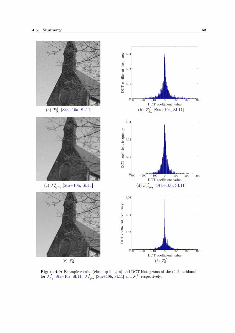
4.5. Summary 63
(a) FJSq
[Sta+10a, SL11]DCT coefficient value
DCT
coeffi
cientfrequen
cy
−300 −200 −100 0 100 200 3000
0.01
0.02
0.03
(b) FJSq
[Sta+10a, SL11]
(c) FJSqSb
[Sta+10b, SL11]DCT coefficient value
DCT
coeffi
cientfrequen
cy
−300 −200 −100 0 100 200 3000
0.01
0.02
0.03
(d) FJSqSb
[Sta+10b, SL11]
(e) FJ0
DCT coefficient value
DCT
coeffi
cientfrequen
cy
−300 −200 −100 0 100 200 3000
0.02
0.04
0.06
(f) FJ0
Figure 4.9: Example results (close-up images) and DCT histograms of the (2, 2) subband,for FJ
Sq[Sta+10a, SL11], FJ
SqSb[Sta+10b, SL11] and FJ
0 , respectively.

64 Chapter 4. Total Variation Based JPEG Anti-Forensics
calibration-based minimization problem is proposed to slightly modify the deblocked JPEGimage but successfully reduce the calibrated feature of KL into the normal range.
Though the proposed method in this chapter does not explicitly handle with the DCT-domain quantization artifacts removal task, the DCT histogram of the resulting anti-forensicimage is to some extent smoothed. Experimental results show that most of the anti-forensicJPEG image FJ
0 is able to pass off as never compressed under the examination of Fan andDe Queiroz’s [FD03] quantization table estimation based detector KQ
F . Besides, Luo et al.’s[LHQ10] quantization step estimation based detector KQ
Luo is also fooled.
Figure 4.10 compares two example DCT histograms of FJSqSb
[Sta+10b, Sta+10a, SL11]
and FJ0 . We can see that the comb-like DCT-domain quantization artifacts still to some extent
exist in FJ0 . This usually happens in the mid-frequency subbands of FJ
0 . This weakness ofFJ0 may potentially be used by advanced JPEG forensic detectors which can expose such kind
of artifacts. In order to cope with the DCT-domain quantization artifacts removal after theJPEG image is processed by the proposed TV-based deblocking operation, we will propose aperceptual DCT histogram smoothing method in Chapter 5. Moreover, the SVM-based JPEGforensic detectors KS100
Li [CS08, LLH12] and KS686P [PBF10] will also be tested.
DCT coefficient value
DCTcoeffi
cientfrequency
−100 −50 0 50 1000
0.02
0.04
0.06
0.08
(a) FJSqSb
[Sta+10b, Sta+10a, SL11]DCT coefficient value
DCTcoeffi
cientfrequency
−150 −100 −50 0 50 100 1500
0.04
0.08
0.12
(b) FJ0
Figure 4.10: Example DCT histograms of the (4, 4) subband, for FJSqSb
[Sta+10a, Sta+10b,
SL11] and FJ0 , respectively.

Chapter 5
JPEG Anti-Forensics with Perceptual
DCT Histogram Smoothing
Contents5.1 Introduction and Motivation . . . . . . . . . . . . . . . . . . . . . . . . . 67
5.2 Proposed JPEG Anti-Forensics . . . . . . . . . . . . . . . . . . . . . . . 69
5.2.1 First-Round TV-Based Deblocking . . . . . . . . . . . . . . . . . . . . . . 69
5.2.2 Perceptual DCT Histogram Smoothing . . . . . . . . . . . . . . . . . . . . 71
5.2.2.1 Disadvantages of Global Laplacian Model . . . . . . . . . . . . . 71
5.2.2.2 Adaptive Local Dithering Signal Model . . . . . . . . . . . . . . 72
5.2.2.3 DCT Histogram Mapping . . . . . . . . . . . . . . . . . . . . . . 76
5.2.2.4 Necessity of First-Round JPEG Deblocking . . . . . . . . . . . . 78
5.2.3 Second-Round TV-Based Deblocking . . . . . . . . . . . . . . . . . . . . . 79
5.2.3.1 Parameter Settings . . . . . . . . . . . . . . . . . . . . . . . . . 79
5.2.3.2 DCT Coefficient Perturbation . . . . . . . . . . . . . . . . . . . 80
5.2.4 De-Calibration . . . . . . . . . . . . . . . . . . . . . . . . . . . . . . . . . 80
5.3 Experimental Results of JPEG Anti-Forensics . . . . . . . . . . . . . . 81
5.3.1 Comparing Anti-Forensic Dithering Methods . . . . . . . . . . . . . . . . 81
5.3.2 Against JPEG Forensic Detectors . . . . . . . . . . . . . . . . . . . . . . . 85
5.3.3 Computation Cost . . . . . . . . . . . . . . . . . . . . . . . . . . . . . . . 87
5.4 Hiding Traces of Double JPEG Compression Artifacts . . . . . . . . . 88
5.4.1 Hiding Traces of Aligned Double JPEG Compression . . . . . . . . . . . . 90
5.4.2 Hiding Traces of Non-Aligned Double JPEG Compression . . . . . . . . . 92
5.4.3 Fooling JPEG Artifacts Based Image Forgery Localization . . . . . . . . . 93
5.5 Summary . . . . . . . . . . . . . . . . . . . . . . . . . . . . . . . . . . . . 94
5.A Appendix: The p.m.f. of the Dithering Signal Using the LaplacianModel . . . . . . . . . . . . . . . . . . . . . . . . . . . . . . . . . . . . . . 98
5.B Appendix: The Constraints Used for Modeling the DCT Coefficients 99
This chapter proposes a JPEG anti-forensic method, which aims at removing from a givenimage the footprints left by JPEG compression, in both the spatial domain and the
DCT domain. With reasonable loss of image quality, the proposed method can defeat existingforensic detectors that attempt to identify traces of the image JPEG compression history orJPEG anti-forensic processing. In the proposed framework, firstly because of a TV-baseddeblocking operation, the partly recovered DCT information is thereafter used to build an
65

66 Chapter 5. JPEG Anti-Forensics with Perceptual DCT Histogram Smoothing
adaptive local dithering signal model which is able to bring the DCT histogram of the processedimage close to that of the original one. Then a perceptual DCT histogram smoothing iscarried out by solving a simplified assignment problem, where the cost function is establishedas the total perceptual quality loss due to the DCT coefficient modification. The second-round deblocking and de-calibration operations successfully bring the image statistics that areused by the JPEG forensic detectors to the normal status. Experimental results show thatthe proposed method outperforms the state-of-the-art methods in a better tradeoff betweenthe JPEG forensic undetectability and the visual quality of processed images. Moreover,the application of the proposed anti-forensic method in disguising double JPEG compressionartifacts is proven to be feasible by experiments.
A paper describing the proposed method was published in an international journal[Fan+14]. The Matlab code of the method is freely shared online and can be downloaded from:http://www.gipsa-lab.grenoble-inp.fr/~wei.fan/documents/AFJPG-TIFS14.tar.gz.

5.1. Introduction and Motivation 67
5.1 Introduction and Motivation
In Chapter 4, a JPEG anti-forensic method based on TV-based deblocking is proposed.Though the method is initially designed to remove spatial-domain blocking artifacts froma JPEG image, experimental results show that it also perturbs the DCT coefficients to theextent that the deblocked JPEG image FJ
0 is able to fool existing quantization artifacts de-tectors. However, it is very difficult to further smooth the DCT histogram of the JPEG imageby simply performing deblocking in the spatial domain while keeping a high visual quality ofthe processed image. As shown in Figure 4.10-(b) and discussed in Section 4.5, though thecomb-like gaps in the DCT histogram of the JPEG image are to some extent filled, the quanti-zation artifacts still exist in FJ
0 in a relatively mild way. These artifacts may not be detectableunder the examination of existing quantization artifacts detectors KQ
F [FD03], KLuo [LHQ10],and KQ
Luo [LHQ10]. Yet, we cannot exclude the possibility of the emergence of other JPEGforensic detectors targeting at this weakness. Therefore, in order to design reliable JPEGanti-forensics, it is necessary to fill the remaining gaps in the DCT histogram of the deblockedJPEG image processed by the TV-based deblocking method presented in Chapter 4.
Here, we adopt a similar strategy to Stamm et al.’s JPEG anti-forensic method [Sta+10a,Sta+10b, SL11] which handles DCT-domain quantization artifacts and spatial-domain block-ing artifacts separately in different domains. Also following the above discussion, in thischapter, we propose a four-step JPEG anti-forensic method, as illustrated in Figure 5.1 andas summarized in the following:
• The first step is the TV-based deblocking in the spatial domain (to be described inSection 5.2.1). This is the same method with that described in Chapter 4, yet withdifferent parameter settings. Besides the removal of JPEG blocking artifacts, anotherpurpose of this step is to partly and plausibly fill gaps in the DCT histogram, so asto facilitate the following step of explicit histogram smoothing. Experimentally, it isnecessary and beneficial to conduct this first-round deblocking, especially for a betterhistogram restoration in the high-frequency subbands where all DCT coefficients arequantized to 0 in the JPEG image (relevant results will be presented in Section 5.2.2.4).After the first step, the image generated from the JPEG image J is denoted as FJ
b .
• We found that in the deblocked image FJb , the comb-like DCT quantization artifacts
are no longer as obvious as those in the JPEG image J (an example is shown in Fig-ure 5.3-(c)). Under the hypothesis that the partly recovered DCT-domain informationis reliable, the next step naturally goes to further filling the remaining gaps in the DCThistogram. This leads us to the construction of an adaptive local model for the DCTcoefficient distribution, with which a perceptual histogram mapping method is there-after proposed to modify the DCT coefficients while minimizing the total SSIM valueloss (to be described in Section 5.2.2). We denote the intermediate image after applyingthe perceptual DCT histogram smoothing as FJ
bq.
• The removal of the DCT quantization artifacts is at the cost of introducing a smallamount of unnatural noise and blocking artifacts in the spatial domain to the output

68 Chapter 5. JPEG Anti-Forensics with Perceptual DCT Histogram Smoothing
image FJbq, despite that we have tried to minimize the image quality loss. Hence, we
move to the spatial domain again and conduct a second-round TV-based deblocking andregularization (to be described in Section 5.2.3). The resulting intermediate image isdenoted as FJ
bqb.
• At last, FJbqb is processed by the de-calibration operation (to be described in Sec-
tion 5.2.4), which is the same with that described in Chapter 4, to generate our anti-forensic JPEG image FJ .
first-round TV-based deblocking
perceptual DCT histogram smoothing
second-round TV-based deblocking
de-calibration
Figure 5.1: The proposed anti-forensic JPEG image creation process for FJ .
By processing a JPEG image alternatively in the spatial domain and in the DCT domain,we hope to create an improved version of anti-forensic JPEG image which achieves betterforensic undetectability than FJ
0 , which is generated by the deblocking based JPEG anti-forensic method in Chapter 4. Meanwhile, by introducing a visual quality control during theproposed DCT histogram smoothing operation, we hope a high quality of the processed imagecan be ensured.
As discussed in Section 1.3.1 and as illustrated in Figure 1.3, one important motiva-tion/application of JPEG anti-forensics is to disguise double JPEG compression artifacts. Inthis chapter, we will also apply the proposed JPEG anti-forensic method in three scenariosof double JPEG compression, to prove the possibility of creating anti-forensic double JPEGcompressed images.
The remainder of this chapter is organized as follows. The proposed JPEG anti-forensicmethod is described in Section 5.2. Section 5.3 shows some experimental results with somecomparisons with the prior art as well as the method proposed in Chapter 4. In Section 5.4,the application of the proposed JPEG anti-forensic method is proven to be practical in creating

5.2. Proposed JPEG Anti-Forensics 69
anti-forensic double JPEG compressed images, with experimental comparisons with the state-of-the-art methods. Finally, we summarize this chapter in Section 5.5.
5.2 Proposed JPEG Anti-Forensics
5.2.1 First-Round TV-Based Deblocking
According to the flowchart of the anti-forensic JPEG image creation shown in Figure 5.1, thefirst step is TV-based deblocking. It is basically what is described in Section 4.3.1, yet inpractice with some different parameter settings. In the proposed TV-based JPEG deblockingmethod, µ in Eq. (4.7), the regularization parameter α in Eq. (A.4), and the step size tk inEq. (4.9) are parameters that we can adjust.
For the setting of the convex set S, we set µ = 1.5 in Chapter 4. Compared with a relativelysmall µ value, it is for better scattering the DCT coefficients in the DCT histogram, so thatthe comb-like quantization artifacts are less likely to appear. Compared with a relativelybig µ value, it is for the image quality consideration of the processed image, because theDCT coefficient is constrained not go too far away from its original quantization bin. Theeffectiveness of this setting is proven by the good forensic undetectability of FJ
0 against thequantization artifacts detectors KQ
F [FD03], KLuo [LHQ10] and KQLuo [LHQ10] with a good
image quality (see Table 4.2 and Figure 4.6). In practice, we found that this setting works wellfor low-frequency and high-frequency subbands, yet the DCT-domain quantization artifactsstill exist in the mid-frequency DCT subbands (see an example in Figure 4.10-(b)).
Different from the setting in Chapter 4, here we set µ = 0.5 for S in order to generateFJb . This setting strictly constrains the processed DCT coefficient to stay within the same
quantization bin as its original value. Besides the visual quality control, this is also favorablefor the perceptual DCT histogram smoothing to be described in Section 5.2.2, where theprocessed DCT coefficient is also constrained to stay within its original quantization bin. Theprojection operator PS works as follows: once a DCT coefficient under processing goes outsidethe quantization bin of its original value, it will be modified back to a random value uniformlydistributed within the quantization bin. In the spatial domain, the resulting pixel values willat last be rounded and truncated to integers in the range [0, 255].
In order to select a good value for α in Eq. (A.4), we create a set of intermediate imagesFJb on UCIDTest92 dataset (see Section 2.3.1 for more descriptions about the datasets) for
comparison. The processed images FJb are generated from the JPEG images for different
values of α ranging from 0.5 to 3 with step 0.5. As the first intermediate image during ouranti-forensic JPEG image creation, the output of the JPEG forensic detectors is not takeninto account for comparison now. We hope FJ
b to have a good image quality and to recoveras much DCT-domain information as possible for the consideration of the further perceptualDCT histogram smoothing. From Figure 5.2-(a) to -(c), the average PSNR, SSIM, and KLdivergence values are respectively compared for different values of α. Note that all the metric

70 Chapter 5. JPEG Anti-Forensics with Perceptual DCT Histogram Smoothing
values are computed using the original image as the reference. We can see that the imagequality, as well as the KL divergence, decreases as α increases. When α > 2.5, the curve ofthe average KL divergence trends to be flat. We therefore only consider α ≤ 2.5, as a highvalue of α will degrade too much the quality of the processed image, with limited improvementon the KL divergence. In the end, we choose α = 1.5 as it appears to have a good tradeoffbetween the DCT histogram restoration quality (which will contribute to the perceptual DCThistogram smoothing described in the Section 5.2.2) and the quality of the processed image.
α
PSNR
0.5 1 1.5 2 2.5 336.6
36.8
37.0
37.2
37.4
37.6
(a) PSNR
α
SSIM
0.5 1 1.5 2 2.5 30.986
0.987
0.988
0.989
0.990
(b) SSIM
α
KLdivergen
ce
0.5 1 1.5 2 2.5 30.08
0.12
0.16
0.20
(c) KL divergence
Figure 5.2: The quality and KL divergence change of the image FJb obtained by the first-
round TV-based deblocking for different values of α. The original image is used as thereference for computing the metric values. Results are obtained on UCIDTest92 dataset.
As to the step size, we set tk = 1/k at the k-th iteration, still following [ADF05].
Similar to the setting in Chapter 4, instead of waiting for the convergence of the opti-mization problem, we select the candidate deblocked image guided by the blocking signaturemeasure KF in Eq. (3.6). Experimentally, we run 50 iterations, and choose the resultingimage giving the smallest KF value as the final result. This provides us with a satisfyingintermediate image FJ
b .
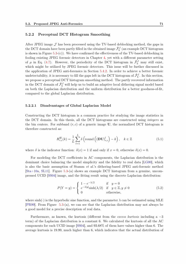
5.2. Proposed JPEG Anti-Forensics 71
5.2.2 Perceptual DCT Histogram Smoothing
After JPEG image J has been processed using the TV-based deblocking method, the gaps inthe DCT domain have been partly filled in the obtained image FJ
b (an example DCT histogramis shown in Figure 5.3-(c)). We have confirmed the effectiveness of the TV-based deblocking infooling existing JPEG forensic detectors in Chapter 4, yet with a different parameter settingof µ in Eq. (4.7). However, the periodicity of the DCT histogram in FJ
b may still exist,which might be utilized by JPEG forensic detectors. This issue will be further discussed inthe application of JPEG anti-forensics in Section 5.4.2. In order to achieve a better forensicundetectability, it is necessary to fill the gaps left in the DCT histogram of FJ
b . In this section,we propose a perceptual DCT histogram smoothing method. The partly recovered informationin the DCT domain of FJ
b will help us to build an adaptive local dithering signal model basedon both the Laplacian distribution and the uniform distribution for a better goodness-of-fit,compared to the global Laplacian distribution.
5.2.2.1 Disadvantages of Global Laplacian Model
Constructing the DCT histogram is a common practice for studying the image statistics inthe DCT domain. In this thesis, all the DCT histograms are constructed using integers asthe bin centers. For subband (r, c) of a generic image U, the normalized DCT histogram istherefore constructed as:
HUr,c(k) =
1
L
L∑
l=1
δ(
round(
(DU)lr,c
)
− k)
, k ∈ Z (5.1)
where δ is the indicator function: δ(x) = 1 if and only if x = 0, otherwise δ(x) = 0.
For modeling the DCT coefficients in AC components, the Laplacian distribution is thedominant choice balancing the model simplicity and the fidelity to real data [LG00], whichis also the basic assumption of Stamm et al.’s dithering-based JPEG anti-forensic method[Sta+10a, SL11]. Figure 5.3-(a) shows an example DCT histogram from a genuine, uncom-pressed UCID [SS04] image, and the fitting result using the discrete Laplacian distribution:
P (Y = y) =
1− e−λ/2 if y = 0
e−λ|y|sinh(λ/2) if y ∈ Z, y 6= 0
0 otherwise,(5.2)
where sinh(·) is the hyperbolic sine function, and the parameter λ can be estimated using MLE[PR99]. From Figure 5.3-(a), we can see that the Laplacian distribution may not always bea good model for a precise description of real data.
Furthermore, as known, the kurtosis (different from the excess kurtosis including a −3term) of the Laplacian distribution is a constant 6. We calculated the kurtosis of all the ACcomponents for each UCID image [SS04], and 93.68% of them have values higher than 6. Theaverage kurtosis is 19.99, much higher than 6, which indicates that the actual distribution of

72 Chapter 5. JPEG Anti-Forensics with Perceptual DCT Histogram Smoothing
DCT coefficient value
DCT
coeffi
cientfrequency
−150 −100 −50 0 50 100 1500
0.04
0.08
0.12
0.16
(a)
DCT coefficient value
DCT
coeffi
cientfrequency
−150 −100 −50 0 50 100 1500
0.2
0.4
0.6
(b)
DCT coefficient value
DCT
coeffi
cientfrequency
−150 −100 −50 0 50 100 1500
0.04
0.08
0.12
0.16
(c)
DCT coefficient value
DCT
coeffi
cientfrequency
−150 −100 −50 0 50 100 1500
0.02
0.04
0.06
0.08
0.1
(d)
Figure 5.3: (a) is the DCT histogram of subband (2, 2) from an example genuine, uncom-pressed UCID image [SS04], and the red curve is the fitting result using the discrete Laplaciandistribution model. Then the image is JPEG compressed with quality factor 50, and theproposed JPEG anti-forensic method is applied. (b), (c), and (d) are the corresponding DCThistograms of (a) in the JPEG image, after the first-round TV-based deblocking, and afterthe adaptive local dithering signal is injected (as described in Section 5.2.2), respectively.
DCT coefficients usually has a much higher peak. This also partly explains the fitting problemof the DCT histogram using the Laplacian model in Figure 5.3-(a).
Moreover, Robertson and Stevenson [RS05] pointed out that for quantized DCT coefficientsthat are observed to be zero, i.e., the DCT coefficients in the quantization bin 0 satisfying(Q(DU))lr,c = 0, the Laplacian model indeed works well. However, for the other DCT coef-ficients in the quantization bin b 6= 0 satisfying (Q(DU))lr,c = b, it appears that the uniformmodel fits better to the real data than the Laplacian model.
5.2.2.2 Adaptive Local Dithering Signal Model
Based on the above analysis, we hope to build a model having a better goodness-of-fit thanthe global Laplacian model. Comparing an example histogram shown in Figure 5.3-(c) with

5.2. Proposed JPEG Anti-Forensics 73
that in -(b), we notice that the DCT-domain information has been partly recovered in FJb ,
with the help of which we will be able to build an adaptive local dithering signal model.
We still use U to denote a generic image pixel value matrix, however U now containspixel values of the processed JPEG image FJ
b using the TV-based deblocking method inSection 5.2.1. For a given DCT subband (r, c) of FJ
b , with Qr,c, the DCT coefficients(DU)lr,c (generically denoted as Y ′) are quantized and then dequantized to obtain coeffi-cients (Q−1(Q(DU)))lr,c (generically denoted as Y ). The goal is to add a dithering signal Nin such a way that the dithered DCT coefficient:
Z = Y +N (5.3)
has no comb-like DCT quantization artifacts while its distribution is to some extent close tothat of Y ′. In this section, we are to find a proper distribution for the dithering signal N .
We firstly consider the AC component. Without special explanation, the DCT coefficientsmentioned in this section are all from the AC component subbands. Inspired by Robertsonand Stevenson’s work about the suitability of the Laplacian model and the uniform model fordifferent parts of the DCT histogram [RS05], we propose an adaptive local dithering signalmodel based on the combination of the Laplacian distribution and the uniform distribution,with the appropriate parameter tuned in each quantization bin.
We denote B−r,c = min
(
(Q(DU))lr,c)
as the non-empty quantization bin with the smallestbin center value, whereas B+
r,c = max(
(Q(DU))lr,c)
as the non-empty quantization bin withthe largest bin center value. We build the dithering signal model through one quantizationbin by another, starting from quantization bin b = 0.
Given quantization bin b, we try to seek for parameter λb of the Laplacian distribution bysolving the following constrained weighted least-squares fitting problem:
λb = arg minλ−
b≤λ≤λ+
b
B+r,cQr,c+⌊
Qr,c
2⌋
∑
k=B−
r,cQr,c−⌊Qr,c
2⌋
wk ×(
HUr,c(k)− P (Y = k)
)2, (5.4)
where HUr,c and P are defined in Eqs. (5.1) and (5.2), respectively. The fitting problem in
Eq. (5.4) means, that we wish to find a local Laplacian distribution which is still close tothe corresponding distribution in FJ
b . We set wk =(
|round( kQr,c
) − b| + 1)−1
as the weightfor the deduction of λb, which emphasizes the importance of the DCT coefficients from thecurrent quantization bin b for the fitting. We also studied some other settings of wk, e.g.,the same function as the one used above but with different powers, the Gaussian function,etc. We found that in practice different settings of wk have minor impact on the histogramrestoration quality, and that the current setting yields slightly better results. Moreover, λ−band λ+b in Eq. (5.4) are the lower and upper bounds of the parameter λ. If λ−b and λ+b are welldefined, then the fitting problem can be established and λb can be found by solving Eq. (5.4);otherwise, the fitting problem cannot be established and we say that λb cannot be found.Before we describe how the searching of the two bounds λ−b and λ+b is performed, we firstexplain the models in use for each quantization bin b.

74 Chapter 5. JPEG Anti-Forensics with Perceptual DCT Histogram Smoothing
If the parameter λb can be found for quantization bin b by solving a well-defined fittingproblem Eq. (5.4), the Laplacian model will be used. In this case, we follow Stamm et al.’sdithering signal model [Sta+10a]. The distribution of the dithering signal N is given by(replacing λ by the actual value of λb):
P (N = n|Y = 0) =
{
c0e−λ|n| if − Qr,c
2 < n <Qr,c
2
0 otherwise,(5.5)
P (N = n|Y = y, y > 0) =
{
c1e−λn if − Qr,c
2 ≤ n < Qr,c
2
0 otherwise,(5.6)
P (N = n|Y = y, y < 0) =
{
c1eλn if − Qr,c
2 < n ≤ Qr,c
2
0 otherwise,(5.7)
with c0 = λ2 (1− e−λQr,c/2)
−1and c1 = λe−λQr,c/2(1− e−λQr,c)
−1. Let P o
m and P em, two
functions of λ, denote the probability mass function (p.m.f.) of the rounded dithering signalwhen Qr,c is an odd number and an even number, respectively. The domain of the p.m.f. isthe integer set {−⌊Qr,c
2 ⌋,−⌊Qr,c
2 ⌋ + 1, · · · , ⌊Qr,c
2 ⌋}. For the sake of brevity, here we omit theequations of the p.m.f., which however can be found in Appendix 5.A. The p.m.f. will be usedlater for the searching of λ−b and λ+b of Eq. (5.4).
As to the quantization bin b, where λb cannot be found, the uniform model will be usedinstead. In this case, the dithering signal N is generated according to:
P (N = n|Y = y) =
{
1Qr,c
if n ∈ N0 otherwise,
(5.8)
where N = (−Qr,c
2 ,Qr,c
2 ) when y = 0, N = [−Qr,c
2 ,Qr,c
2 ) when y > 0, and N = (−Qr,c
2 ,Qr,c
2 ]
when y < 0.
Now, we go back to the searching of the bounds λ−b and λ+b used in Eq. (5.4). We start fromthe center of the DCT histogram, i.e., quantization bin b = 0. We set λ−b = 10−3 according toValenzise et al.’s statement [VTT11] that the parameter λ of the Laplacian model usually takesvalues between 10−3 and 1 for natural images. The constraint used in the searching is basedon the observation that in the distribution of DCT coefficients, the probability decreases whenthe coefficient magnitude increases. As an example and as illustrated in Figure 5.4, when Qr,c
is an odd number, we constrain that the probability of DCT coefficient falling in the leftmostinteger bin k = −⌊Qr,c
2 ⌋ (or the rightmost integer bin k = ⌊Qr,c
2 ⌋) of the quantization binb = 0 should be no smaller than either that in the rightmost integer bin of the quantizationbin b = −1 or that in the leftmost integer bin of the quantization bin b = 1. For the moment,in the neighboring quantization bins −1 and 1, the DCT coefficients are assumed to followa uniform distribution. Then λ+b is determined by solving Eq. (5.9), where M0,M−1,M1
are respectively the approximate probabilities of DCT coefficient falling in quantization bins0,−1, 1, which are estimated directly from the constructed histogram. The searching forλ+b can be done using a numerical method. A set of numbers are uniformly sampled from

5.2. Proposed JPEG Anti-Forensics 75
the interval [10−3, 1]. Given each number in this set as the parameter λ, P om is calculated.
Therefore, λ+b is chosen as the largest number satisfying constraints in Eq. (5.9). When Qr,c isan even number, the procedure to find λ+b is similar yet slightly different. Detailed informationcan be found in Appendix 5.B.
λ+b = arg max10−3≤λ≤1
λ, subject to: P om
(
N = ⌊Qr,c
2⌋|Y = 0
)
×M0 ≥ max
(
M−1
Qr,c,M1
Qr,c
)
(5.9)
quantization bin
Figure 5.4: Illustration for the constraint used for the searching of λ+b when Qr,c is anodd number: The probability for the leftmost (or the rightmost) integer bin of the quanti-zation bin b = 0 should be no smaller than either that of the rightmost integer bin in thequantization bin b = −1 or that of the leftmost integer bin in the quantization bin b = 1.
For quantization bins b = 1, 2, · · · , B+r,c, we adopt a similar procedure to obtain λ−b and
λ+b . The constraint is that the probability of coefficients falling in the leftmost integer bin ofquantization bin b ≥ 1 should be no bigger than that in the rightmost integer bin of quantiza-tion bin b− 1, meanwhile the probability of coefficients falling in the rightmost integer bin ofquantization bin b should be no smaller than that in the leftmost integer bin of quantizationbin b + 1. The distribution in the quantization bin b − 1 is already defined at that moment,and for the quantization bin b+ 1 we assume the uniform distribution. Then λ−b and λ+b arechosen as the smallest and largest number in [10−3, λb−1] satisfying the constraint, respec-tively. However, if λ−b and λ+b cannot be found, the uniform model in Eq. (5.8) will be used asthe dithering signal model for the current and following quantization bin(s). For quantizationbins b = −1,−2, · · · , B−
r,c, a similar searching procedure for the values of λ−b and λ+b is applied(see Appendix 5.B for details).
When we have well defined λ−b and λ+b values, the parameter λb of the Laplacian model isobtained by solving the minimization problem in Eq. (5.4), and the dithering signal N can bethereafter generated according to Eqs. (5.5)-(5.7); otherwise, the uniform model in Eq. (5.8)is used. Algorithm 5.1 summarizes the proposed adaptive local dithering procedure for theAC components.

76 Chapter 5. JPEG Anti-Forensics with Perceptual DCT Histogram Smoothing
Algorithm 5.1 Adaptive local dithering procedure for AC components.
1: require: Y2: initialization: Z = Y3: for b = 0, 1, 2, · · · , B+
r,c,−1,−2, . . . , B−r,c do
4: Search for λ+b and λ−b (e.g., using Eq. (5.9))5: if λ+b and λ−b are well defined then6: λb ← Eq. (5.4)7: Generate N using Eq. (5.5)/(5.6)/(5.7)8: Z ← Z +N9: else
10: Generate N using Eq. (5.8)11: Z ← Z +N12: end if13: end for14: return Z
Although we adopt Stamm et al.’s [Sta+10a, SL11] dithering signal model, note that theirmodel is rather global and our model is local. In Stamm et al.’s model, once the parameter λof the Laplacian distribution is estimated for a subband, it will be used for all the quantizationbins of this subband. However, in our model, it is considered locally for each quantization bin b.We tune parameter λb of the Laplacian model for different quantization bins if it can be found;otherwise, the uniform model will be used instead. Moreover, in Stamm et al.’s method, theMLE [PR99] is used to estimate λ from the JPEG image. However, in the proposed method,λb for each quantization bin is obtained via a weighted least-squares fitting using the post-processed image FJ
b where the DCT-domain information is partly recovered. We will showin Section 5.3.1 that our method leads to a better restoration of the DCT histogram of theoriginal, uncompressed image.
Because there is no general model for the DC component, we use the uniform model forall the quantization bins to generate the dithering signal N according to Eq. (5.8).
For each quantization bin, the dithering signal generated by numerical sampling of a givenprobability distribution function can reproduce the natural, fine-grained details in the DCThistogram. An example result is shown in Figure 5.3-(d).
5.2.2.3 DCT Histogram Mapping
Now, we can generate the dithered signal Z using the adaptive local dithering signal model.However, we cannot use Z directly as the altered DCT coefficients by adding the ditheringsignal N randomly to Y , without any consideration of the image spatial-domain information:the processed image will suffer from low visual quality as Stamm et al.’s anti-forensic JPEGimage does [Sta+10a, SL11]. A different strategy is adopted here. We will try to move thedistribution of Y ′ (i.e., the distribution of DCT coefficients of FJ
b ) towards that of Z, whileminimizing the introduced distortion in the spatial domain, by solving an assignment problem

5.2. Proposed JPEG Anti-Forensics 77
whose cost function is defined as the total perceptual quality loss.
We still consider the DCT coefficients in each quantization bin individually. In this section,all the DCT coefficients mentioned are in a single quantization bin b of subband (r, c). Aclassical assignment problem can be established as follows. Let Ob denote the set of DCTcoefficients in quantization bin b from Y ′ which are to be modified, and T b is used to denotethe set of target DCT coefficient values from Z (= Y +N) falling in the quantization bin b.Ob and T b are of equal size. The weight function W : Ob × T b → R is defined as the SSIMvalue loss due to the coefficient modification, compared with the currently achieved processedimage from the last solved assignment problem (or FJ
b at the very beginning). Our goal is tofind a bijection f : Ob → T b such that the cost function:
∑
o∈Ob
W (o, f(o)), (5.10)
is minimized. This problem can be solved using the well-known Hungarian algorithm13 [Kuh55](see Section 2.4.2 for more descriptions of this algorithm). The solution of the assignmentproblem can be found in O(D3) time, where D is the dimensionality of the problem. If D issmall, the problem however can be solved within a reasonable time. The setting of D will befurther discussed in Section 5.3.1.
In order to save the computation cost, we hereby propose three strategies to simplify thebuilding and the solving of this assignment problem. Firstly, not all but only part of the DCTcoefficients in Y ′ are to be modified, so that the dimensionality of the assignment problem canbe largely reduced. For choosing the DCT coefficients to put into Ob, first we compare theunnormalized DCT histogram (using integers as bin centers) of Y ′, denoted as hbo, and thatof Z, denoted as hbt . Integers bQr,c − ⌊Qr,c
2 ⌋, bQr,c − ⌊Qr,c
2 ⌋+ 1, · · · , bQr,c + ⌊Qr,c
2 ⌋ are all thepossible rounded DCT coefficient values in hbo and hbt . It is obvious that the dithering processin Section 5.2.2.2 ensures that the two histograms in comparison have the same number ofDCT coefficients. We compute their difference histogram as:
hbd(k) = hbo(k)− hbt(k), k = bQr,c − ⌊Qr,c
2⌋, · · · , bQr,c + ⌊
Qr,c
2⌋. (5.11)
In order to reduce the dimensionality of the assignment problem, the first strategy is that wedo not modify the coefficients in hbo that are already in the correct integer bin with respect tohbt . More precisely, for each integer bin k with hbd(k) ≤ 0, the corresponding DCT coefficientsare left unchanged; and for each integer bin k with hbd(k) > 0, instead of putting all the hbo(k)coefficients in Ob, we only put hbd(k) (< hbo(k)) coefficients into Ob while leaving the other hbt(k)coefficients unchanged. In general, this will yield suboptimal results, however the advantageis that it will largely reduce the computation cost with still satisfactory final results. In orderto control the distortion in the spatial domain, it is better to choose the DCT coefficientwhose corresponding spatial-domain 8 × 8 block is less sensitive to noise for being altered.Using a similar strategy with [BFT12], here we adopt the SSIM index [Wan+04] to compute
13We use the Matlab code downloaded from: http://www.mathworks.fr/matlabcentral/fileexchange/
20652-hungarian-algorithm-for-linear-assignment-problems-v2-3.

78 Chapter 5. JPEG Anti-Forensics with Perceptual DCT Histogram Smoothing
a similarity map between the currently achieved image and FJb . The DCT coefficients whose
spatial-domain 8× 8 block has a higher SSIM index value are chosen to be modified and putinto set Ob. Note that at the very beginning of the procedure, the SSIM index cannot becomputed because the currently achieved image is exactly FJ
b . In this case, we calculate thelocal variance instead. We also have to reduce the dimensionality of the target value set T b
so that Ob and T b are of equal size. To this end, for each k with hbd(k) < 0, in Z we randomly
choose −hbd(k) (> 0) values among the DCT coefficients whose rounded values are k, and putthese values into T b.
The second strategy to simplify the building of the assignment problem in Eq. (5.10) isto speed up the calculation of the weight function W . Normally, for each DCT coefficient oin Ob, all the possible modifications to values in T b should be enforced to calculate the cost.Yet, this can be simplified by only computing the SSIM value loss when the DCT coefficiento in Ob is changed to a value in T b which is the farthest from o. The linear interpolation isafterwards used to estimate the cost for all the other possible modifications in T b.
The last strategy is to randomly split the simplified assignment problem into several smallerones of lower dimensionality which can be solved in a reasonable time. This will be furtherdiscussed with experimental results in Section 5.3.1, where we also show that the adoption ofall these strategies will not impair the visual quality of the obtained image, despite the factthat these strategies lead to suboptimal solutions.
After solving a simplified assignment problem for each quantization bin, we are able tosmooth the DCT histogram with minimum introduced distortion in the spatial domain. Thecreated intermediate image is denoted as FJ
bq.
5.2.2.4 Necessity of First-Round JPEG Deblocking
As one may have noticed, it is possible to perform the perceptual DCT histogram smoothingdescribed in this section directly on the JPEG image, without the application of the first-round TV-based deblocking described in Section 5.2.1. Here, FJ
q denotes the image obtainedusing the proposed perceptual DCT histogram smoothing directly from the JPEG image J .For comparing FJ
bq and FJq , we conduct a test on UCIDTest92 dataset.
PSNR, SSIM are adopted as the image quality evaluation metrics (see Section 2.2.2 formore descriptions). In order to give a quantitative evaluation of the DCT histogram, we usethe KL divergence (see Section 2.2.3 for more descriptions) as the difference measure betweenthe histogram of the uncompressed image and the one of the processed image. A smaller valueof KL divergence means a better resemblance between the two compared histograms. Table5.1 reports the average PSNR, SSIM, and KL divergence values of FJ
bq and FJq . All the metric
values are computed using the original uncompressed image I as the reference. The differencebetween the two kinds of KL divergences is that the first one is averaged over the subbandswhere not all the DCT coefficients are quantized to 0 in the original JPEG image, whereas theother is averaged over the rest of the subbands. The lower KL divergence value of FJ
bq than

5.2. Proposed JPEG Anti-Forensics 79
that of FJq demonstrates that with the partly recovered DCT-domain information in FJ
b weare able to achieve a more accurate DCT histogram restoration, especially for the subbandswhere all the DCT coefficients are quantized to 0 in JPEG images.
Table 5.1: Image quality and KL divergence (with I as the reference) comparison af-ter the perceptual DCT histogram smoothing, with and without the first-round TV-baseddeblocking. Results are obtained on UCIDTest92 dataset.
PSNR SSIM KL divergence-1 KL divergence-2
FJbq 36.4419 0.9862 0.0904 0.1054
FJq 36.1427 0.9874 0.1316 0.2622
Moreover, FJb also helps us to reduce the dimensionality of the simplified assignment
problem during the DCT histogram mapping described in Section 5.2.2.3. The reason is thatin the first strategy of simplifying the assignment problem, more DCT coefficients in FJ
b willalready be in the correct integer bin than those in the JPEG image.
Furthermore, FJbq achieves a slightly higher PSNR value, but slightly lower SSIM value,
than FJq . Considering the results of both metrics, the two kinds of images have comparable
visual qualities. Another advantage of the TV-based deblocking is the removal of JPEGblocking artifacts. It is therefore necessary to conduct the first-round TV-based deblockingfor a better tradeoff between the visual quality and the histogram restoration quality of theprocessed image.
5.2.3 Second-Round TV-Based Deblocking
In the perceptual DCT histogram smoothing, although we have tried to modify the DCTcoefficients while minimizing the spatial-domain distortion, there must be some unnaturalnoise and blocking artifacts introduced in FJ
bq. Hence, we focus on the spatial domain againand propose to apply the second-round TV-based deblocking and regularization.
5.2.3.1 Parameter Settings
Similar to Section 5.2.1, the deblocking procedure is basically the same as that described inSection 4.3.1, yet with some modifications to the parameter setting. Since the JPEG blockingartifacts presented in FJ
bq are not as serious as those in J , hence we lower the parameters α(see Eq. (A.4)) and tk (see Eq. (4.9)) for a milder JPEG deblocking. We set α = 0.9, and thestep size tk = 1/(k + 1) at the k-th iteration. As to the setting of the convex set S, here weset µ = 1.5 (see Eq. (4.7)), which constrains that the processed DCT coefficient should staywithin the same or the neighboring quantization bins as its original value. Once a processedDCT coefficient goes outside of the constrained range, the projection operator PS modifiesits value back to a random value uniformly distributed in the original quantization bin. Thiscan avoid strong DCT histogram shape modification by the TV-based deblocking and prevent

80 Chapter 5. JPEG Anti-Forensics with Perceptual DCT Histogram Smoothing
the emergence of new DCT quantization artifacts. Using these empirical parameter settings,experimentally we can achieve satisfactory results considering both the forensic undetectabilityand the visual quality of the processed image.
5.2.3.2 DCT Coefficient Perturbation
We also observed that in practice, the TV-based deblocking might interfere with the output ofthe quantization table estimation based detector KQ
F [FD03], especially in the high-frequencysubbands. The image tends to be over-smoothed by the TV-based regularization. As analyzedin Section 4.2.1, the quantization table estimation based detector will detect one DCT subbandas quantized by 3 instead of 1, when the probability of DCT coefficients whose rounded valuesare integer multiples of 3 (denoted as p0) is higher than 67.28%. This frequently happens inthe high-frequency subbands of relatively smooth images, which has a high frequency of DCTcoefficients with rounded value 0.
In order to tackle this problem, we propose to introduce a slight perturbation to the DCTcoefficients in the high-frequency subbands which have a high value of p0 during each opti-mization iteration. Considering the influence of the subgradient method, the DCT coefficientsprojection of PS , and the pixel value rounding and truncation in the spatial domain, for agiven DCT subband, if p0 > 60%, we modify part of the DCT coefficients whose roundedvalues are 0 to the integer bins −5,−4, · · · ,−1, 1, 2, · · · , 5. The DCT coefficient whose cor-responding spatial-domain block has a higher tolerance of distortion (measured by the SSIMindex comparing the currently achieved image and the deblocked image in the last subgradi-ent iteration, or FJ
bq at the very beginning) will be modified first to a DCT coefficient whichhas a bigger rounded amplitude. The modification constrains that the relative probability ofinteger bins −5,−4, · · · ,−1, 1, 2, · · · , 5 should stay unchanged. The modification stops oncep0 reaches 50%.
In order to avoid over-smoothing of the image, a random threshold for each image is drawnfrom the distribution of the KF values for genuine, uncompressed images, and the iterationstops once the KF value in Eq. (3.6) decreases below it. Otherwise, if this cannot be achievedwithin 30 iterations, the resulting intermediate image with the smallest KF output is chosenas the final result. The created image after this step is denoted as FJ
bqb.
5.2.4 De-Calibration
For FJbqb, all the existing detectors seems to be well fooled except the calibrated feature based
detector KL [LB11]. Based on the same consideration presented in Section 4.3.2, we performthe de-calibration operation to the intermediate image FJ
bqb. The method is the same asthat described in Section 4.3.2. In order to avoid tedious repetition, here we refrain fromre-presenting it. After de-calibration, the anti-forensic JPEG image FJ is obtained.

5.3. Experimental Results of JPEG Anti-Forensics 81
5.3 Experimental Results of JPEG Anti-Forensics
Besides the state-of-the-art anti-forensic JPEG images listed in Table 3.2 and FJ0 created in
Chapter 4, our improved anti-forensic JPEG image and two kinds of intermediate results arecreated from the JPEG image J :
• FJ , with the application of the proposed four-step JPEG anti-forensic method;
• FJbq, with the application of the proposed first-round TV-based deblocking and the per-
ceptual DCT histogram smoothing method, the maximum dimensionality is set to be200 when solving the assignment problem;
• F ′bq, the creation of which is the same as FJ
bq, except that there is no limit set for themaximum dimensionality when solving the assignment problem.
5.3.1 Comparing Anti-Forensic Dithering Methods
Figure 5.5 shows the SSIM value (with the original image I as the reference) comparisonwhen tested on the “Lena” image. Note that the difference between the results shown hereand those shown in [VTT11] is probably due to the different versions of “Lena” images in useand to the different parameter settings of SSIM index. However, the trend of the curves is inaccordance with each other, and the results confirm the conclusion of [VTT11] that it is noteasy to conceal the traces of JPEG compression without serious image quality loss. Accordingto Figure 5.5, the perceptual anti-forensic dither of Valenzise et al. [VTT11] is able to achievea higher SSIM value of the processed image than Stamm et al.’s anti-forensic dither [Sta+10a,SL11]. However, the proposed DCT histogram smoothing method outperforms both of them[Sta+10a, SL11, VTT11] in terms of SSIM value. Figure 5.7 shows the close-up images ofLena. In the relatively smooth area of the image, e.g., the shoulder and the face of Lena, wecan see that less noise is introduced in the spatial domain of FJ
bq compared with FJSq
and FJV .
The average PSNR and SSIM values of large-scale test on UCIDTest dataset for FJbq are
35.9926 dB and 0.9872, respectively, which are noticeably higher than those of FJSq
and of
FJV (see Table 5.4). It demonstrates that the proposed perceptual DCT histogram smoothing
can help us to achieve a higher image quality of the processed image than the state-of-the-artanti-forensic dithering methods [Sta+10a, SL11, VTT11].
In the proposed DCT histogram smoothing method, we have to solve an assignment prob-lem for each quantization bin of each subband. As mentioned in Section 5.2.2.3, the computa-tion cost is O(D3) when using the Hungarian algorithm [Kuh55], whereD is the dimensionalityof the assignment problem. Obviously, the problem solving might be impractical when D istoo large. A possible solution is that we randomly split a single assignment problem intoseveral smaller ones. From Figure 5.5, we can see that the problem splitting barely affectsthe image quality of the processed image. However, it largely saves the computation cost to

82 Chapter 5. JPEG Anti-Forensics with Perceptual DCT Histogram Smoothing
Quality factor
SSIM
50 55 60 65 70 75 80 85 90 95
0.96
0.97
0.98
0.99
1
J
FJSq
FJV
FJbq
F ′bq
Figure 5.5: SSIM values achieved by J , FJSq
[Sta+10a, SL11], FJV [VTT11], FJ
bq, and F ′
bq,
with I as the reference, when tested on the “Lena” image. The FJbq plot is almost under
that of F ′
bq.
Quality factor
Computationcost
(inseconds)
50 55 60 65 70 75 80 85 90 95100
200
300
400F
Jbq
F′
bq
Figure 5.6: Time taken to create FJbq, and F ′
bq from the JPEG compressed “Lena” imagewith different quality factors. By reducing the dimensionality of the assignment problem, thecomputation cost is largely reduced to conduct the perceptual DCT histogram smoothing.
conduct the perceptual DCT histogram smoothing procedure, as demonstrated by the teston the “Lena” image, as reported in Figure 5.6. In the large-scale test, in order to speed upthe simulation, we always randomly split the assignment problem into several smaller ones ofmaximum dimensionality of 200.
With experiments carried out on UCIDTest dataset, we compute the KL divergence valuebetween I and FJ
Sq, and that between I and FJ
bq for all DCT subbands. The difference betweenthese two KL divergence values is reported in Table 5.2. We notice that during the ditheringprocess, the subband where all the coefficients are quantized to 0 is left untouched in [Sta+10a,

5.3. Experimental Results of JPEG Anti-Forensics 83
(a) J (b) FJSq
(c) FJV (d) FJ
bq
Figure 5.7: Example results (close-up images) of FJbq compared with J , FJ
Sq[Sta+10a,
SL11], and FJV [VTT11], where J is compressed with quality factor 50. Their SSIM values
(with I as the reference) are: (a) 0.9809, (b) 0.9509, (c) 0.9610, and (d) 0.9731. We cansee that less noise is introduced in FJ
bq especially in the relatively smooth area of the image.Results are obtained on the “Lena” image.
SL11]. To be fair for FJSq
, these subbands were not counted in the comparison. From Table
5.2, we can see that FJbq performs consistently better than FJ
Sq. Similar results are obtained
when compared with Valenzise et al.’s anti-forensic JPEG images FJV [VTT11], because the
dithering model used in [VTT11] is exactly the same as in [Sta+10a] in the DCT domain.We can conclude that the proposed adaptive local dithering model has a better restorationcapability of the original DCT histogram than the one based on the global Laplacian model[Sta+10a, VTT11].
We also compare the KL divergence value between I and FJ0 obtained using the anti-
forensic method presented in Chapter 4, and that between I and FJ for all DCT subbands.The difference between these two KL divergence values is reported in Table 5.3. In this

84 Chapter 5. JPEG Anti-Forensics with Perceptual DCT Histogram Smoothing
Table 5.2: The difference of the KL divergence between I and FJSq
[Sta+10a, SL11], and
that between I and FJbq for all 64 DCT subbands. The average difference value over all
subbands is 0.0552 with standard deviation 0.0249. For a fair comparison for FJSq
, thesubbands, whose DCT coefficients are all quantized to 0 in the JPEG image J , are notcounted. Results are obtained on UCIDTest dataset.
rc 1 2 3 4 5 6 7 8
1 0.0001 0.0065 0.0118 0.0278 0.0493 0.0634 0.0663 0.0656
2 0.0042 0.0166 0.0229 0.0363 0.0447 0.0565 0.0504 0.0369
3 0.0161 0.0208 0.0291 0.0442 0.0573 0.0665 0.0634 0.0497
4 0.0200 0.0317 0.0409 0.0470 0.0658 0.0802 0.0553 0.0446
5 0.0357 0.0395 0.0522 0.0678 0.0764 0.0930 0.0927 0.0856
6 0.0441 0.0383 0.0642 0.0610 0.0726 0.0769 0.0806 0.0957
7 0.0538 0.0442 0.0678 0.0595 0.0879 0.0809 0.0948 0.0975
8 0.0619 0.0545 0.0697 0.0528 0.0927 0.0880 0.0854 0.0722
comparison, all the DCT subbands of all the images in UCIDTest dataset are considered, nomatter whether there are some DCT subbands whose coefficients are all quantized to 0 in thecorresponding JPEG image J . We can see that the JPEG anti-forensic method proposed inthis chapter has improved the DCT histogram recovery performance compared to the methodpresented in Chapter 4. We can conclude that the perceptual DCT histogram smoothingmethod proposed in Section 5.2.2 is able to better shape the DCT histogram towards that ofthe original image.
Table 5.3: The difference of the KL divergence between I and FJ0 , and that between I and
FJ for all 64 DCT subbands. The average difference value over all subbands is 0.0160 withstandard deviation 0.0139. All the subbands are considered, no matter whether the DCTcoefficients are all quantized to 0 in the JPEG image J . Results are obtained on UCIDTestdataset.
rc 1 2 3 4 5 6 7 8
1 -0.0040 0.0002 0.0047 0.0035 0.0072 0.0135 0.0243 0.0464
2 0.0045 -0.0043 -0.0002 0.0053 0.0127 0.0275 0.0248 0.0451
3 0.0023 -0.0033 0.0037 0.0106 0.0136 -0.0042 0.0001 0.0292
4 0.0060 0.0013 0.0094 0.0132 0.0258 0.0186 0.0288 0.0395
5 0.0035 0.0088 0.0113 0.0254 0.0121 0.0071 0.0128 0.0278
6 0.0109 0.0202 -0.0065 0.0193 0.0138 0.0139 0.0143 0.0291
7 0.0287 0.0298 -0.0036 0.0231 0.0132 0.0151 0.0130 0.0297
8 0.0435 0.0487 0.0243 0.0408 0.0287 0.0281 0.0294 0.0035

5.3. Experimental Results of JPEG Anti-Forensics 85
5.3.2 Against JPEG Forensic Detectors
Table 5.4 reports the AUC values achieved by different kinds of (anti-forensic) JPEG imagesagainst 7 scalar-based forensic detectors listed in Table 3.1. Besides, the last two columnsof Table 5.4 also list the average PSNR and SSIM values for the comparison of the visualquality of processed image with the original uncompressed image I as the reference. Moreover,Figure 5.8 plots the ROC curves obtained by Stamm et al.’s [Sta+10a, Sta+10b, SL11] anti-forensic JPEG image FJ
SqSband ours FJ .
Table 5.4: From the 2nd to the 8th columns, the AUC values for different kinds of imageswhen tested against different scalar-based JPEG forensic detectors are listed; the imagequality (with I as the reference) comparison is reported in the last 2 columns. Results areobtained on UCIDTest dataset.
KF KLuo KQLuo KV KL K1
U K2U PSNR SSIM
J 0.9991 1.0000 0.9996 0.9976 0.9811 0.9860 0.8840 37.0999 0.9919
FJSq
0.9332 0.4328 0.7328 0.9977 0.9946 0.9633 0.9483 33.4061 0.9756
FJSqSb
0.3783 0.0806 0.6288 0.8337 0.5338 0.6309 0.4854 30.4591 0.9509
FJV 0.9889 0.4330 0.8066 0.9834 0.9958 0.9916 0.9574 33.2890 0.9802
FJSu 0.8802 0.9772 0.9475 0.1115 0.9610 0.7052 0.3149 31.6552 0.9719
FJ0 0.6756 0.6046 0.5194 0.6210 0.4490 0.6772 0.5880 35.4814 0.9843
FJb 0.7590 0.4830 0.4354 0.8542 0.9588 0.6813 0.5650 36.7405 0.9891
FJbq 0.9170 0.4050 0.5244 0.8435 0.9874 0.8081 0.6531 35.9926 0.9872
FJ 0.5398 0.6425 0.4598 0.6159 0.4344 0.5894 0.5317 35.9855 0.9866
False positive rate
Truepositiverate
0 0.2 0.4 0.6 0.8 10
0.2
0.4
0.6
0.8
1
KF
KLuo
KQLuo
KV
KL
K1U
K2U
Random guess
False positive rate
Truepositiverate
0 0.2 0.4 0.6 0.8 10
0.2
0.4
0.6
0.8
1
KF
KLuo
KQLuo
KV
KL
K1U
K2U
Random guess
(a) FJSqSb
[Sta+10a, Sta+10b, SL11] (b) FJ
Figure 5.8: ROC curves achieved by FJ and FJSqSb
[Sta+10a, Sta+10b, SL11] againstJPEG forensic detectors. Results are obtained on UCIDTest dataset.
From both Table 5.4 and the ROC curves shown in Figure 5.8, we can see that our anti-
86 Chapter 5. JPEG Anti-Forensics with Perceptual DCT Histogram Smoothing
forensic JPEG image has a better forensic undetectability compared with Stamm et al.’s FJSqSb
.
The other version of Stamm et al.’s anti-forensic JPEG image FJSq
processed by the DCThistogram smoothing can be well detected by the JPEG forensic detectors which were designedtargeting at it [Val+11, LB11]. The anti-forensic JPEG image FJ
V created by the perceptualanti-forensic dithering [VTT11] has a similar anti-forensic performance as FJ
Sq, while achieving
a higher SSIM value on average. The median filtering based deblocking [Sta+10b] improvesthe undetectability of the anti-forensic JPEG image FJ
SqSbagainst forensic detectors, but with
a PSNR value loss of 6.64 dB on average, compared to JPEG image J (see the last 2 columnsof Table 5.4).
Figure 5.8-(b) shows that the proposed method succeeds in fooling all the 3 JPEG blockingdetectors, yet through the minimization of a different TV-based blocking measure in Eq. (4.6).Our method is also capable of fooling the advanced detector KV [Val+11, VTT13]. The reasonmight be that the TV term in Eq. (4.4) manages to suppress the unnatural noises utilizedby this detector. Furthermore, the calibration-based detector KL [LB11] is defeated by thede-calibration operation. Even though the quantization table estimation based detector KQ
F
is proven to be not very reliable in Section 4.2.1, we still test it on our anti-forensic JPEGimages FJ on UCIDTest dataset, 93.70% of which can be passed off as never JPEG compressed(making the true positive rate be 6.30%). Our method successfully fools existing detectors, atthe cost of a slightly lower visual quality than the JPEG compressed image: 1.11 dB of PSNRloss and 0.0053 of SSIM value loss on average. Compared to Stamm et al.’s anti-forensic JPEGimage FJ
SqSb[Sta+10a, Sta+10b, SL11], our method achieves a better tradeoff between the
forensic undetectability and the visual quality of processed images: the average PSNR hasbeen improved by 5.53 dB and 0.0357 of SSIM gain has been achieved; meanwhile our methodachieves a better overall forensic undetectability.
Concerning the SVM-based detectors KS100Li [CS08, LLH12], and KS686
P [PBF10] whichare initially designed for steganalysis, we follow the experimental setup described in Sec-tion 2.2.1.2. The AUC value as a function of the image replacement rate for different kindsof images, is shown in Figure 5.9. We can see that our anti-forensic JPEG image FJ doesnot perform the best when tested by KS100
Li and KS686P . However, unlike FJ
V or FJSqSb
, the
performance of FJ is quite stable and in general quite satisfactory when compared with otheranti-forensic images. Meanwhile, FJ
0 created using the method described in Chapter 4 slightlyoutperforms FJ . This is understandable, as we explicitly smooth DCT histograms for creatingFJ , which may lead to more changes in image statistics. When the replacement rate is about0.10, the performance of our anti-forensic JPEG image is quite good, with a relatively lowAUC value of the SVM-based detectors. In this case, we can safely replace a 112× 160 blockin a 384 × 512 UCID image. This is enough for many image forgery creation scenarios, e.g.,replacing the head of one person in the picture. We remain reserved on whether the proposedJPEG anti-forensic method is able to disguise a whole JPEG image as uncompressed, as itcan still be well detected using machine learning based forensic methods. However, it is stillhighly applicable in various JPEG anti-forensic scenarios, e.g., image splicing, and disguisingdouble JPEG compression artifacts (see results in Section 5.4).
Figure 5.10 shows the anti-forensic JPEG images created from an example JPEG image

5.3. Experimental Results of JPEG Anti-Forensics 87
Replacement rate
AUC
0 0.1 0.2 0.3 0.4 0.5 0.6 0.8 10.5
0.6
0.7
0.8
0.9
1
J
FJSq
FJSqSb
FJV
FJSu
FJ0
FJ
(a) KS100Li [CS08, LLH12]
Replacement rate
AUC
0 0.1 0.2 0.3 0.4 0.5 0.6 0.8 10.5
0.6
0.7
0.8
0.9
1
J
FJSq
FJSqSb
FJV
FJSu
FJ0
FJ
(b) KS686P [PBF10]
Figure 5.9: The AUC value as a function of image replacement rate for different kindsof images, when tested using the SVM-based detectors. Results are obtained by testing onUCIDTE dataset and training on UCIDTR dataset.
with quality factor 50. As expected, Figure 5.10-(d) processed using the proposed JPEGanti-forensic method better preserves the image details and the edges than -(c). It can alsobe observed that even after the deblocking operation [Sta+10b, SL11], the spatial-domainnoise introduced by the dithering signal [Sta+10a, SL11] can still be noticed in the smoothareas of the image in -(c). Some example DCT histograms of the anti-forensic JPEG imagein Figure 5.10-(d) are shown in Figure 5.11: no noticeable artifacts appear.
5.3.3 Computation Cost
Table 5.5: Comparison of the average time taken to create different kinds of anti-forensicJPEG images. Results are obtained on UCIDTest92 dataset.
FJSq
FJSqSb
FJV FJ
Su FJ0 FJ
in second(s) 0.0503 0.0879 0.4380 0.0201 7.0815 176.8205
Table 5.5 records the average time taken for the generation of different anti-forensic JPEGimages on UCIDTest92 dataset, using Matlab R2012b, on a PC with 24G RAM and 2.80GHzCPU. We can see that the proposed JPEG anti-forensic method requires around 3 minutesto create an anti-forensic JPEG image on average, using the unoptimized Matlab code. Thebottleneck of the computation cost lies in the perceptual DCT histogram smoothing, as thecomputation cost is O(D3) using the Hungarian algorithm. However, the reduction of thedimensionality of the assignment problem discussed in Section 5.3.1 can effectively lower thecomputation cost. Apparently, the proposed method is more complex and more computation-ally demanding compared to other state-of-the-art JPEG anti-forensic methods. However,the benefit is a better tradeoff between the forensic undetectability and the image quality asshown in Section 5.3.2. Moreover, in practice, usually the forger does not need to create a

88 Chapter 5. JPEG Anti-Forensics with Perceptual DCT Histogram Smoothing
(a) I (b) J
(c) FJSqSb
[Sta+10a, Sta+10b, SL11] (d) FJ
Figure 5.10: Example results (close-up images) of FJ compared with I, J , and FJSqSb
[Sta+10a, Sta+10b, SL11], where J is compressed with quality factor 50. Our anti-forensicJPEG image FJ has a better image quality compared with FJ
SqSb.
large amount of image forgeries. It is therefore acceptable to take several minutes to generatean anti-forensic JPEG image.
5.4 Hiding Traces of Double JPEG Compression Artifacts
As JPEG is one of the most commonly used image compression formats today, it is a very likelyscenario that a forger alters something in a JPEG image and re-saves it using the JPEG formatagain. As explained in Section 1.3.1, this will lead to double JPEG compression artifacts whichmay be utilized by forensic investigators. An investigator may wish to tell whether an imagehas been double JPEG compressed (exposing aligned or non-aligned double JPEG compressionartifacts), and furthermore which part of the image has been altered (forgery localization via

5.4. Hiding Traces of Double JPEG Compression Artifacts 89
DCT coefficient value
DCT
coeffi
cientfrequen
cy
−400 −300 −200 −100 0 100 200 300 4000
0.01
0.02
0.03
0.04
DCT coefficient value
DCT
coeffi
cientfrequen
cy
−80 −60 −40 −20 0 20 40 60 800
0.05
0.1
0.15
0.2
0.25
(a) (2, 2) (b) (6, 4)
DCT coefficient value
DCT
coeffi
cientfrequen
cy
−60 −40 −20 0 20 40 600
0.05
0.1
0.15
0.2
0.25
0.3
0.35
DCT coefficient value
DCT
coeffi
cientfrequen
cy
−15 −10 −5 0 5 10 150
0.05
0.1
0.15
0.2
0.25
0.3
0.35
(c) (3, 7) (d) (8, 8)
Figure 5.11: Example DCT histograms of different subbands of an anti-forensic JPEGimage FJ shown in Figure 5.10-(d). No noticeable comb-like DCT quantization artifactsappear in the histograms.
analysis of double JPEG compression artifacts). In the following, we show how our JPEGanti-forensic method can be used to deceive three state-of-the-art image forensic algorithms[PF08, BP12a, BP12b] that take advantage of double JPEG compression artifacts.
In this section, single JPEG compressed images are only JPEG compressed with qualityfactor QF2, while double JPEG compressed images are firstly JPEG compressed with qualityfactor QF1 and JPEG compressed again with quality factor QF2. Image cropping or contentmodification may occur between the two compressions. For anti-forensic testing, the JPEGanti-forensic methods in [Sta+10a, Sta+10b, SL11, VTT11, SS11] and the proposed JPEGanti-forensic methods in both Chapter 4 and this chapter are applied on the JPEG image afterthe first compression with QF1. Then the anti-forensic JPEG image is unchanged, croppedby a random grid shift, or partly altered. Finally the resulting image is JPEG compressedagain with QF2 to create anti-forensic double JPEG compressed image.
We conduct large-scale tests on UCID corpus [SS04], while following the experimental

90 Chapter 5. JPEG Anti-Forensics with Perceptual DCT Histogram Smoothing
settings in the original papers of double JPEG detectors [PF08, BP12a, BP12b]. Every datasetcontains double JPEG compressed images first with QF1 and then with QF2 between whichthere might be JPEG anti-forensics applied, cropping, or partial image replacement accordingto different scenarios. In Section 5.4.1 and Section 5.4.2, each dataset also includes single JPEGcompressed images with QF2. In order to avoid tedious repetition later, we hereby explainthe naming rule of the image datasets we will use in this section. Unless otherwise stated, thedataset created from UCIDTE or UCIDTest100 (see Section 2.3.1 for more descriptions aboutthe datasets) is written in bold letters. The end of the name of the dataset ‘-R’ indicateswhich kind of (or no) JPEG anti-forensics is applied to the single JPEG compressed imagewith QF1 before further processing. It can the followings:
• ‘-T’: no JPEG anti-forensics is applied;
• ‘-S’: Stamm et al.’s dithering based JPEG anti-forensic method [Sta+10a, SL11] is ap-plied;
• ‘-SS’: Stamm et al.’s dithering [Sta+10a, SL11] and median filtering based JPEG anti-forensic method [Sta+10b, SL11] is applied;
• ‘-V’: Valenzise et al.’s perceptual dithering based JPEG anti-forensic method [VTT11]is applied;
• ‘-Su’: Sutthiwan and Shi’s SAZ attack [SS11] is applied;
• ‘-F0’: our previously proposed TV-based anti-forensic method in Chapter 4 is applied;
• ‘-F’: the proposed four-step JPEG anti-forensic method in this chapter is applied.
5.4.1 Hiding Traces of Aligned Double JPEG Compression
In [PF08], Pevný and Fridrich proposed a method using the SVM with feature vectors formedby DCT histograms in the low-frequency subbands to classify single and double JPEG com-pressed images. For constructing the feature vector, they consider 9 low-frequency AC sub-bands, and for each of them a 16-bin histogram is computed. The 144-dimensional featurevectors are then fed to an SVM.
In order to train the SVM-based A-DJPG (Aligned Double JPEG) compression detector[PF08], each image in UCIDTR is firstly JPEG compressed with the primary quality factorQF1 and then compressed again with the secondary quality factor QF2 6= QF1 to create theA-DJPG compressed images. Here, QF1 ∈ {50, 56, 63, 69, 81, 88, 94}, and QF2 = 75, following[PF08]. The single JPEG compressed images are created by JPEG compressing the originaluncompressed images with QF2. Then we have 7× 500 + 500 = 4000 images for training thedetector, using the LIBSVM [CL11].
Each UCIDTE image is firstly JPEG compressed with QF1, and then compressed againwith QF2 to create the A-DJPG compressed images. During the two JPEG compressions,

5.4. Hiding Traces of Double JPEG Compression Artifacts 91
anti-forensic operations may occur. Meanwhile, each UCIDTE image is JPEG compressedonce with QF2 for creating the single JPEG compressed image. For forensic testing, we create7 datasets each of which has 4000 images as well. The name of the dataset follows the patternA-DJPG-R.
The ROC curves in Figure 5.12 show that the proposed method successfully masks thepresence of double JPEG compression artifacts. The AUC value of the A-DJPG compressiondetector [PF08] is decreased to 0.4832 for A-DJPG-F from 0.9274 for the training datasetand 0.9152 for A-DJPG-T. Other state-of-the-art JPEG anti-forensic methods [Sta+10a,Sta+10b, VTT11, SS11] as well as the one proposed in Chapter 4 achieve similar anti-forensicperformance, however with higher image quality loss than the proposed method in this chapter,as reported in Table 5.6. Among different anti-forensic double JPEG compressed images, ouranti-forensic images have the highest visual quality (with the uncompressed image as thereference).
False Positive Rate
TruePositiveRate
0 0.2 0.4 0.6 0.8 10
0.2
0.4
0.6
0.8
1
training dataset
A-DJPG-T
A-DJPG-S
A-DJPG-SS
A-DJPG-V
A-DJPG-Su
A-DJPG-F0
A-DJPG-F
Random guess
Figure 5.12: ROC curves achieved on A-DJPG-R against the SVM-based A-DJPG com-pression detector [PF08]. Results are obtained by testing on UCIDTE dataset and trainingon UCIDTR dataset. All the JPEG anti-forensic methods in consideration are able to movethe ROC curves close to the random guess line.
Table 5.6: Image quality (with the uncompressed image as the reference) comparison of(anti-forensic) double JPEG compressed images created from UCIDTE for different datasetsA-DJPG-R. A-DJPG-F achieves the best image quality among different anti-forensicdouble JPEG compressed images in comparison.
-T -S -SS -V -Su -F0 -F
PSNR 35.0916 32.8974 30.4112 32.8090 31.0414 34.1906 34.4417
SSIM 0.9879 0.9690 0.9463 0.9762 0.9664 0.9800 0.9821

92 Chapter 5. JPEG Anti-Forensics with Perceptual DCT Histogram Smoothing
5.4.2 Hiding Traces of Non-Aligned Double JPEG Compression
Bianchi and Piva [BP12a] analyzed the statistical change in the DCT coefficients of the DCcomponent, after a JPEG image is compressed again with a non-aligned 8× 8 grid. A simplebut powerful threshold detector is constructed [BP12a], which is based on measuring thenon-uniformity of a suitably defined integer periodicity map of the DC coefficients.
We compress each UCIDTE image with QF1, then the JPEG image is croppedwith a random shift (i, j) 6= (0, 0), with 0 ≤ i, j ≤ 7. At last the cropped im-age is JPEG compressed again with QF2 to create the NA-DJPG (Non-Aligned Dou-ble JPEG) compressed image. Meanwhile each UCIDTE image is JPEG compressedonce with QF2 for creating the single JPEG compressed image. Anti-forensic oper-ation may occur after the first JPEG compression with QF1. For forensic testing,we create 7 datasets whose names follow the pattern NA-DJPG-R. Here, as sug-gested in [BP12a], QF1 ∈ {50, 53, 56, 59, 63, 66, 69, 72, 75, 78, 81, 84, 88, 91, 94} and QF2 ∈{50, 53, 56, 59, 63, 66, 69, 72, 75, 78, 81, 84, 88, 91, 94, 97}, yielding in total 15 × 16 = 240 dif-ferent quality factor combinations for creating NA-DJPG compressed images. Therefore, wehave 15× 16× 500 + 16× 500 = 128000 images for each dataset.
QF2
AUC
50 60 70 80 90 1000.5
0.6
0.7
0.8
0.9
1NA-DJPG-TNA-DJPG-S
NA-DJPG-SS
NA-DJPG-V
NA-DJPG-SuNA-DJPG-F0
NA-DJPG-F
Figure 5.13: Average AUC value of the NA-DJPG compression detector [BP12a] as afunction of QF2, when tested on NA-DJPG-R, created from UCIDTE. The improvementof forensic undetectability of NA-DJPG-F over NA-DJPG-F0 shows the necessity ofconducting the DCT histogram smoothing.
For each quality factor pair (QF1, QF2), the single JPEG compressed images togetherwith their corresponding (anti-forensic) double JPEG compressed images are tested using theNA-DJPG detector [BP12a]. Then the AUC value can be computed for different kinds ofimages. Figure 5.13 shows the average AUC value over quality factor QF1, under a fixed valueof QF2. We can see that FJ
Sq[Sta+10a, SL11], FJ
SqSb[Sta+10b, SL11], both of which have
DCT histograms explicitly smoothed, keep a good forensic undetectability against this NA-DJPG detector. Although our previous JPEG anti-forensic method described in Chapter 4can successfully fool many existing JPEG forensic detectors (as shown in Figure 4.6 and

5.4. Hiding Traces of Double JPEG Compression Artifacts 93
Table 5.4), the gaps in the DCT domain are not well filled (an example can be seen inFigure 4.10-(b)), which might be exposed by the NA-DJPG compression detector [BP12a].Similarly, anti-forensic double JPEG compressed images created from FJ
Su [SS11] can also bedetected, to some extent, by the NA-DJPG compression detector [BP12a], especially whenQF2 is high. By contrast, with the application of the proposed JPEG anti-forensic method,the AUC of the NA-DJPG detector [BP12a] is successfully kept close to 0.5 (random guess).This proves the necessity of an explicit DCT histogram smoothing for JPEG anti-forensicsand the effectiveness of the proposed perceptual histogram smoothing method, because nointeger periodicity can be detected by the NA-DJPG detector in the DCT histogram of ouranti-forensic double JPEG compressed images.
Besides a good forensic undetectability, the proposed anti-forensic method is able to createanti-forensic NA-DJPG compressed images with the highest image quality among all 6 kindsof anti-forensic images (see results in Table 5.7).
Table 5.7: Image quality (with the uncompressed image as the reference) comparison of(anti-forensic) double JPEG compressed images created from UCIDTE for different datasetsNA-DJPG-R. NA-DJPG-F achieves the best image quality among different anti-forensicdouble JPEG compressed images in comparison.
-T -S -SS -V -Su -F0 -F
PSNR 34.6098 32.7958 30.2825 32.4824 30.9379 33.8345 34.0929
SSIM 0.9319 0.8650 0.8487 0.8864 0.8898 0.9168 0.9222
5.4.3 Fooling JPEG Artifacts Based Image Forgery Localization
Bianchi and Piva [BP12b] derived a likelihood-map indicating the probability for each 8 × 8
block of being double JPEG compressed, under the hypothesis of the presence of A-DJPG orNA-DJPG compression artifacts in the tampered image.
We conduct the test on the 100 images in the UCIDTest100 dataset. Following [BP12b],we first compress each UCIDTest100 image with QF1; the resulting image is partly replacedusing the original uncompressed image, and then compressed again with QF2. After theprimary JPEG compression, image cropping and/or anti-forensics may occur. In total, 7×6 =
42 datasets are created considering 7 kinds of images and 6 different scenarios. We namethe dataset as LOC-E -DJPG-K/L-R, where the italic letters may change to representdifferent scenarios. E can be ‘A’, or ‘NA’. ‘NA’ indicates that before the second compressionthe image is cropped by a random shift (i, j) 6= (0, 0), 0 ≤ i, j ≤ 7; whereas ‘A’ meansthere is no image cropping happening. K/L indicates how much portion of the image hasundergone double JPEG compression, which also implies how much portion of the imagehas been replaced by the original uncompressed image before the second JPEG compression.When K/L is ‘1/2’, it indicates the left half of the image is replaced using the originalimage; when K/L is ‘15/16’, the central 1/16 portion of the image is replaced; when K/Lis ‘1/16’, the whole image except its central 1/16 portion is replaced. In all datasets, QF1

94 Chapter 5. JPEG Anti-Forensics with Perceptual DCT Histogram Smoothing
and QF2 are taken from {50, 56, 63, 69, 75, 81, 88, 94} and {50, 56, 63, 69, 75, 81, 88, 94, 100},respectively. Therefore each dataset has 8× 9× 100 = 7200 images.
Figure 5.14 shows the average AUC value over all possible QF1 (under a fixed value ofQF2) achieved by the detector [BP12b] for the different scenarios and different kinds of images.Note that the results shown here are computed from the standard map instead of the simplifiedmap (see [BP12b] for details). The blue curves demonstrate the effectiveness of the detectorwhen no JPEG anti-forensics is applied after the first compression. With the help of JPEGanti-forensics, the forgery localization detector [BP12b] can be well fooled. Our anti-forensicdouble JPEG compressed image again achieves the best image visual quality among all kindsof anti-forensic images (see Tables 5.8-5.13).
Table 5.8: Image quality (with the uncompressed image as the reference) comparisonof (anti-forensic) double JPEG compressed images created from UCIDTest100 for differ-ent datasets LOC-A-DJPG-15/16-R. LOC-A-DJPG-15/16-F achieves the best imagequality among different anti-forensic double JPEG compressed images in comparison.
-T -S -SS -V -Su -F0 -F
PSNR 35.5248 33.5597 30.8639 33.4702 31.5678 34.5200 34.8080
SSIM 0.9875 0.9744 0.9528 0.9786 0.9703 0.9798 0.9819
Table 5.9: Image quality (with the uncompressed image as the reference) comparisonof (anti-forensic) double JPEG compressed images created from UCIDTest100 for differentdatasets LOC-NA-DJPG-15/16-R. LOC-NA-DJPG-15/16-F achieves the best imagequality among different anti-forensic double JPEG compressed images in comparison.
-T -S -SS -V -Su -F0 -F
PSNR 35.1211 33.1837 30.8331 32.9189 31.4694 34.3396 34.5884
SSIM 0.9395 0.8776 0.8726 0.8972 0.9067 0.9265 0.9308
Table 5.10: Image quality (with the uncompressed image as the reference) comparisonof (anti-forensic) double JPEG compressed images created from UCIDTest100 for differentdatasets LOC-A-DJPG-1/2-R. LOC-A-DJPG-1/2-F achieves the best image qualityamong different anti-forensic double JPEG compressed images in comparison.
-T -S -SS -V -Su -F0 -F
PSNR 36.3810 34.7737 32.7724 34.7288 33.2466 35.6653 35.8817
SSIM 0.9897 0.9829 0.9713 0.9852 0.9799 0.9855 0.9866
5.5 Summary
In this chapter, we propose a novel perceptual DCT histogram smoothing method to improvethe TV-based deblocking based JPEG anti-forensic method described in Chapter 4. Theproposed JPEG anti-forensic method designs four steps to alternatively remove the artifacts

5.5. Summary 95
QF2
AUC
50 60 70 80 90 100
0.4
0.5
0.6
0.7
0.8
0.9
1LOC-A-DJPG-15/16-T
LOC-A-DJPG-15/16-S
LOC-A-DJPG-15/16-SS
LOC-A-DJPG-15/16-V
LOC-A-DJPG-15/16-Su
LOC-A-DJPG-15/16-F0
LOC-A-DJPG-15/16-F
(a) LOC-A-DJPG-15/16-R
QF2
AUC
50 60 70 80 90 100
0.4
0.5
0.6
0.7
0.8
0.9
1LOC-NA-DJPG-15/16-T
LOC-NA-DJPG-15/16-S
LOC-NA-DJPG-15/16-SS
LOC-NA-DJPG-15/16-V
LOC-NA-DJPG-15/16-Su
LOC-NA-DJPG-15/16-F0
LOC-NA-DJPG-15/16-F
(b) LOC-NA-DJPG-15/16-R
QF2
AUC
50 60 70 80 90 100
0.4
0.5
0.6
0.7
0.8
0.9
1LOC-A-DJPG-1/2-T
LOC-A-DJPG-1/2-S
LOC-A-DJPG-1/2-SS
LOC-A-DJPG-1/2-V
LOC-A-DJPG-1/2-Su
LOC-A-DJPG-1/2-F0
LOC-A-DJPG-1/2-F
(c) LOC-A-DJPG-1/2-R
QF2
AUC
50 60 70 80 90 100
0.4
0.5
0.6
0.7
0.8
0.9
1LOC-NA-DJPG-1/2-T
LOC-NA-DJPG-1/2-S
LOC-NA-DJPG-1/2-SS
LOC-NA-DJPG-1/2-V
LOC-NA-DJPG-1/2-Su
LOC-NA-DJPG-1/2-F0
LOC-NA-DJPG-1/2-F
(d) LOC-NA-DJPG-1/2-R
QF2
AUC
50 60 70 80 90 100
0.4
0.5
0.6
0.7
0.8
0.9
1LOC-A-DJPG-1/16-T
LOC-A-DJPG-1/16-S
LOC-A-DJPG-1/16-SS
LOC-A-DJPG-1/16-V
LOC-A-DJPG-1/16-Su
LOC-A-DJPG-1/16-F0
LOC-A-DJPG-1/16-F
(e) LOC-A-DJPG-1/16-R
QF2
AUC
50 60 70 80 90 100
0.4
0.5
0.6
0.7
0.8
0.9
1LOC-NA-DJPG-1/16-T
LOC-NA-DJPG-1/16-S
LOC-NA-DJPG-1/16-SS
LOC-NA-DJPG-1/16-V
LOC-NA-DJPG-1/16-Su
LOC-NA-DJPG-1/16-F0
LOC-NA-DJPG-1/16-F
(f) LOC-NA-DJPG-1/16-R
Figure 5.14: Average AUC value as a function of QF2 of the forgery localization detec-tor [BP12b], when tested on LOC-E-DJPG-K/L-R, created from UCIDTest100. Theblack curves with triangles indicating AUC values around 0.5, prove the effectiveness ofthe proposed four-step JPEG anti-forensic method in masking double JPEG compressionartifacts.
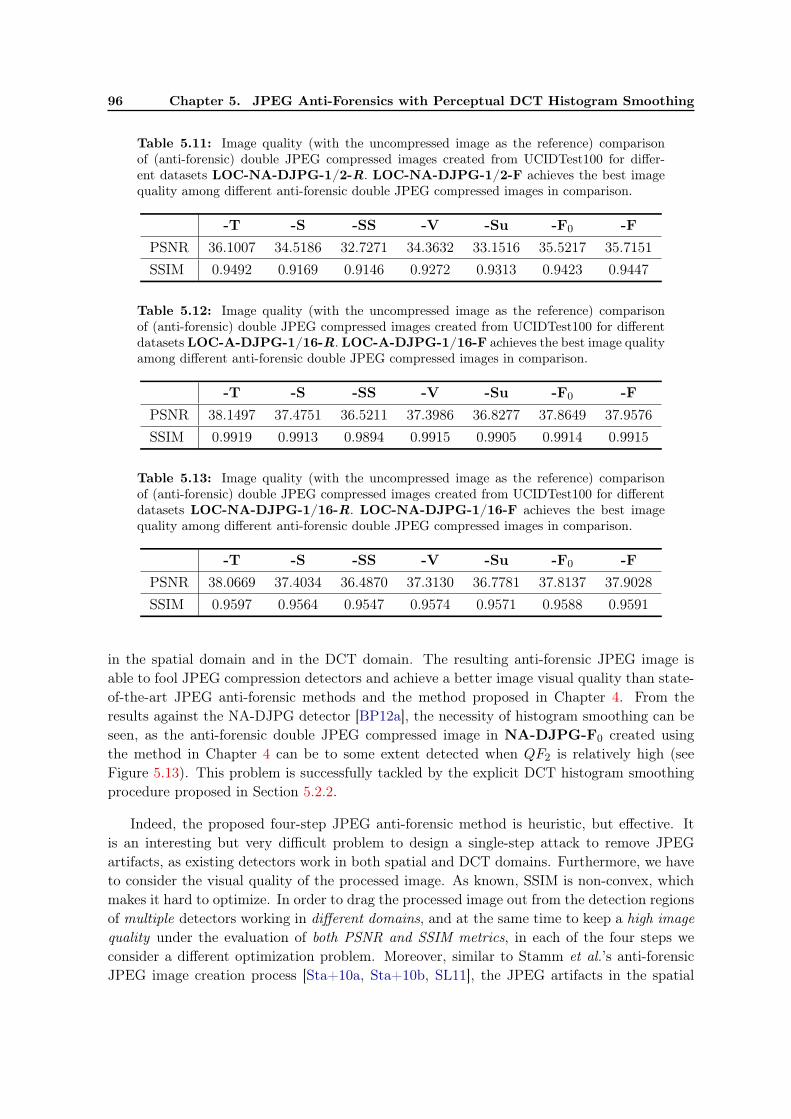
96 Chapter 5. JPEG Anti-Forensics with Perceptual DCT Histogram Smoothing
Table 5.11: Image quality (with the uncompressed image as the reference) comparisonof (anti-forensic) double JPEG compressed images created from UCIDTest100 for differ-ent datasets LOC-NA-DJPG-1/2-R. LOC-NA-DJPG-1/2-F achieves the best imagequality among different anti-forensic double JPEG compressed images in comparison.
-T -S -SS -V -Su -F0 -F
PSNR 36.1007 34.5186 32.7271 34.3632 33.1516 35.5217 35.7151
SSIM 0.9492 0.9169 0.9146 0.9272 0.9313 0.9423 0.9447
Table 5.12: Image quality (with the uncompressed image as the reference) comparisonof (anti-forensic) double JPEG compressed images created from UCIDTest100 for differentdatasets LOC-A-DJPG-1/16-R. LOC-A-DJPG-1/16-F achieves the best image qualityamong different anti-forensic double JPEG compressed images in comparison.
-T -S -SS -V -Su -F0 -F
PSNR 38.1497 37.4751 36.5211 37.3986 36.8277 37.8649 37.9576
SSIM 0.9919 0.9913 0.9894 0.9915 0.9905 0.9914 0.9915
Table 5.13: Image quality (with the uncompressed image as the reference) comparisonof (anti-forensic) double JPEG compressed images created from UCIDTest100 for differentdatasets LOC-NA-DJPG-1/16-R. LOC-NA-DJPG-1/16-F achieves the best imagequality among different anti-forensic double JPEG compressed images in comparison.
-T -S -SS -V -Su -F0 -F
PSNR 38.0669 37.4034 36.4870 37.3130 36.7781 37.8137 37.9028
SSIM 0.9597 0.9564 0.9547 0.9574 0.9571 0.9588 0.9591
in the spatial domain and in the DCT domain. The resulting anti-forensic JPEG image isable to fool JPEG compression detectors and achieve a better image visual quality than state-of-the-art JPEG anti-forensic methods and the method proposed in Chapter 4. From theresults against the NA-DJPG detector [BP12a], the necessity of histogram smoothing can beseen, as the anti-forensic double JPEG compressed image in NA-DJPG-F0 created usingthe method in Chapter 4 can be to some extent detected when QF2 is relatively high (seeFigure 5.13). This problem is successfully tackled by the explicit DCT histogram smoothingprocedure proposed in Section 5.2.2.
Indeed, the proposed four-step JPEG anti-forensic method is heuristic, but effective. Itis an interesting but very difficult problem to design a single-step attack to remove JPEGartifacts, as existing detectors work in both spatial and DCT domains. Furthermore, we haveto consider the visual quality of the processed image. As known, SSIM is non-convex, whichmakes it hard to optimize. In order to drag the processed image out from the detection regionsof multiple detectors working in different domains, and at the same time to keep a high image
quality under the evaluation of both PSNR and SSIM metrics, in each of the four steps weconsider a different optimization problem. Moreover, similar to Stamm et al.’s anti-forensicJPEG image creation process [Sta+10a, Sta+10b, SL11], the JPEG artifacts in the spatial

5.5. Summary 97
domain and the DCT domain are considered alternatively. With a local modification to theimage considering multiple metrics, we are able to create anti-forensic JPEG images with agood tradeoff between the forensic undetectability and the image quality.
In Chapters 4-5, the proposed JPEG anti-forensic methods are inspired by the TV-basedJPEG image post-processing [ADF05]. The TV can be considered as a simple but effectiveimage prior. Besides, in the proposed TV-based JPEG deblocking framework, there is nolikelihood term considering the JPEG compression process as in the MAP-based JPEG post-processing methods [RS05, SC07]. In the literature of image restoration, there exist moresophisticated image prior models [RS05, SC07, ZW11] than the TV, and spatial-domain com-pression noise model for JPEG compression [RS05]. In Chapter 6, still following the researchline of designing image anti-forensics leveraging on image restoration, we will propose an-other JPEG anti-forensic method using a more advanced image prior than the TV and witha likelihood term modeling the JPEG compression process.

98 Chapter 5. JPEG Anti-Forensics with Perceptual DCT Histogram Smoothing
5.A Appendix: The p.m.f. of the Dithering Signal Using theLaplacian Model
Here, we only consider AC components of the image. The probability density function (p.d.f.)of the distribution of the dithering signal N is denoted as P (N = n|Y = y). P can be easilycomputed (see Eqs. (5.5)-(5.7)) according to the sign of the quantized DCT coefficient Y .Here, the p.m.f. of the rounded dithering signal are calculated with domain defined as theinteger set {−⌊Qr,c
2 ⌋,−⌊Qr,c
2 ⌋+ 1, · · · , ⌊Qr,c
2 ⌋}. Eqs. (5.12)-(5.13) below are the p.m.f. of therounded dithering signal for quantization bin 0 when Qr,c is an odd number and an evennumber, respectively. For quantization bin b 6= 0, the p.m.f. of the rounded dithering signalare listed in Eqs. (5.14)-(5.17) according to the sign and the parity of b.
P om(N = n|Y = 0) =
2c0λ−1(
1− e−λ/2)
if n = 0
−c0λ−1e−λ(n+1/2)(
1− eλ)
if n = 1, · · · , ⌊Qr,c
2 ⌋c0λ
−1eλ(n+1/2)(
1− e−λ)
if n = −⌊Qr,c
2 ⌋, · · · ,−10 otherwise,
(5.12)
P em(N = n|Y = 0) =
2c0λ−1(
1− e−λ/2)
if n = 0
−c0λ−1e−λQr,c/2(
1− eλ/2)
if n = −Qr,c
2 ,Qr,c
2
−c0λ−1e−λ(n+1/2)(
1− eλ)
if n = 1, · · · , Qr,c
2 − 1
c0λ−1eλ(n+1/2)
(
1− e−λ)
if n = −Qr,c
2 + 1, · · · ,−10 otherwise,
(5.13)
P om(N = n|Y = y, y > 0) =
{
−c1λ−1e−λ(n+1/2)(
1− eλ)
if n = −⌊Qr,c
2 ⌋, · · · , ⌊Qr,c
2 ⌋0 otherwise,
(5.14)
P em(N = n|Y = y, y > 0) =
c1λ−1eλQr,c/2
(
1− e−λ/2)
if n = −Qr,c
2
−c1λ−1e−λQr,c/2(
1− eλ/2)
if n =Qr,c
2
−c1λ−1e−λ(n+1/2)(
1− eλ)
if n = −Qr,c
2 + 1, · · · , Qr,c
2 − 1
0 otherwise,(5.15)
P om(N = n|Y = y, y < 0) =
{
c1λ−1eλ(n+1/2)
(
1− e−λ)
if n = −⌊Qr,c
2 ⌋, · · · , ⌊Qr,c
2 ⌋0 otherwise,
(5.16)
P em(N = n|Y = y, y < 0) =
−c1λ−1e−λQr,c/2(
1− eλ/2)
if n = −Qr,c
2
c1λ−1eλQr,c/2
(
1− e−λ/2)
if n =Qr,c
2
c1λ−1eλ(n+1/2)
(
1− e−λ)
if n = −Qr,c
2 + 1, · · · , Qr,c
2 − 1
0 otherwise.(5.17)

5.B. Appendix: The Constraints Used for Modeling the DCT Coefficients 99
5.B Appendix: The Constraints Used for Modeling the DCTCoefficients
In Section 5.2.2.2, for building the adaptive local dithering signal model for AC components,we combine the Laplacian model and the uniform model together. A key point to establish theadaptive local model for the dithering signal is that we try to find an appropriate parameterλb of the Laplacian model for each quantization bin b. If we cannot find a valid value forλb, the uniform model is used instead for the current and following quantization bin(s). Theparameter λb is derived by solving a constrained weighted least-squares fitting problem (seeEq. (5.4)), with λb bounded between λ−b and λ+b . In Section 5.2.2.2, we show how to searchfor the bound λ+b (λ−b is set as 10−3) for quantization bin 0 when Qr,c is an odd number, usinga numerical method. Here we explain how to search for the two bounds in other cases.
In the quantization bin 0 when Qr,c is an even number
The empirical observation tells us that in the distribution of DCT coefficients of AC com-ponent, the probability of DCT coefficient decreases when the coefficient magnitude increases.Now we consider the quantization bin 0 when Qr,c is an even number.
quantization bin
Figure 5.15: For the quantization bin 0, the probability of DCT coefficient falling in theleftmost (or rightmost) integer bin should be no smaller than either that in the rightmostinteger bin of quantization bin −1 or that in the leftmost integer bin of quantization bin 1.
As illustrated in Figure 5.15, the probability of DCT coefficient falling in the leftmost (orrightmost) integer bin should be no smaller than either that in the rightmost integer bin ofquantization bin −1 or that in the leftmost integer bin of quantization bin 1. For the moment,the neighboring quantization bins −1 and 1 are assumed to follow a uniform distribution.Similarly to the case in the quantization bin 0 when Qr,c is an odd number, we still set

100 Chapter 5. JPEG Anti-Forensics with Perceptual DCT Histogram Smoothing
λ−b = 10−3, whereas λ+b can be found by solving:
λ+b = arg max10−3≤λ≤1
λ,
subject to: P em
(
N =Qr,c
2 − 1|Y = 0)
×M0
≥ P em
(
N =Qr,c
2 |Y = 0)
×M0 +12 max
(
M−1
Qr,c, M1
Qr,c
)
(5.18)
using a numerical method. Note that Mb (b = B−r,c, B
−r,c+1, · · · , B+
r,c) denotes the approximateprobability that the DCT coefficient falls in quantization bin b.
In the quantization bin b > 0
As illustrated in Figures 5.16-(a) and -(b), we consider a quantization bin b > 0, whenQr,c is an odd number and an even number, respectively. The probability of DCT coefficientfalling in the leftmost integer bin of quantization bin b should be no bigger than that in therightmost integer bin of quantization bin b−1. Meanwhile, the probability of DCT coefficientfalling in the rightmost integer bin of quantization bin b should be no smaller than that inthe leftmost integer bin of quantization bin b + 1. As the building of the dithering signalmodel is an iterative procedure, the distribution of the dithering signal N in the quantizationbin b − 1 has already been estimated in the last iteration. Hence, P o
m(N = n|Y = b − 1) orP em(N = n|Y = b− 1) is known. Moreover, for the quantization bin b+ 1, its dithering signal
is assumed to follow a uniform distribution for the moment. Therefore, when Qr,c is an oddnumber, the constraints that λ−b and λ+b can be respectively found by solving:
λ−b = arg min10−3≤λ≤λb−1
λ
subject to:
P om
(
N = −⌊Qr,c
2 ⌋|Y = b)
×Mb ≤ P om
(
N = ⌊Qr,c
2 ⌋|Y = b− 1)
×Mb−1
P om
(
N = ⌊Qr,c
2 ⌋|Y = b)
×Mb ≥ Mb+1
Qr,c,
(5.19)and
λ+b = arg max10−3≤λ≤λb−1
λ
subject to:
P om
(
N = −⌊Qr,c
2 ⌋|Y = b)
×Mb ≤ P om(N = ⌊Qr,c
2 ⌋|Y = b− 1)×Mb−1
P om
(
N = ⌊Qr,c
2 ⌋|Y = b)
×Mb ≥ Mb+1
Qr,c.
(5.20)

5.B. Appendix: The Constraints Used for Modeling the DCT Coefficients 101
quantization bin
(a) Qr,c is an odd number
quantization bin
(b) Qr,c is an even number
Figure 5.16: For the quantization bin b > 0, the probability of DCT coefficient falling inthe leftmost integer bin should be no bigger than that in the rightmost integer bin of theneighboring quantization bin b − 1, meanwhile the probability of coefficients falling in therightmost integer bin of quantization bin b should be no smaller than that in the leftmostinteger bin of quantization bin b+ 1.
Similarly, λ−b and λ+b are respectively defined as:
λ−b = arg min10−3≤λ≤λb−1
λ
subject to:
P em
(
N = −Qr,c
2 + 1|Y = b)
×Mb ≤ P em
(
N = −Qr,c
2 |Y = b)
×Mb
+P em
(
N =Qr,c
2 |Y = b− 1)
×Mb−1
P em
(
N =Qr,c
2 − 1|Y = b)
×Mb ≥ P em
(
N =Qr,c
2 |Y = b)
×Mb +Mb+1
2Qr,c,
(5.21)

102 Chapter 5. JPEG Anti-Forensics with Perceptual DCT Histogram Smoothing
and
λ+b = arg max10−3≤λ≤λb−1
λ
subject to:
P em
(
N = −Qr,c
2 + 1|Y = b)
×Mb ≤ P em
(
N = −Qr,c
2 |Y = b)
×Mb
+P em
(
N =Qr,c
2 |Y = b− 1)
×Mb−1
P em
(
N =Qr,c
2 − 1|Y = b)
×Mb ≥ P em
(
N =Qr,c
2 |Y = b)
×Mb +Mb+1
2Qr,c,
(5.22)when Qr,c is an even number.
In other words, using a numerical method, λ−b and λ+b are found respectively as the smallestand largest number in the interval [10−3, λb−1] satisfying certain constraints. Note that λb−1
is estimated from the last iteration. If λ−b and λ+b cannot be found, the uniform model will beadopted for the current and following quantization bin(s).
In the quantization bin b < 0
For the quantization bin b < 0, the procedure of building the dithering signal model isvery similar to that for quantization bin b > 0. For the sake of simplicity, we do not presentthe details here, but only give the equations for searching λ−b and λ+b , that are:
λ−b = arg min10−3≤λ≤λb+1
λ
subject to:
P om
(
N = −⌊Qr,c
2 ⌋|Y = b)
×Mb ≥ Mb−1
Qr,c
P om
(
N = ⌊Qr,c
2 ⌋|Y = b)
×Mb ≤ P om(N = −⌊Qr,c
2 ⌋|Y = b+ 1)×Mb+1,
(5.23)and
λ+b = arg max10−3≤λ≤λb+1
λ
subject to:
P om
(
N = −⌊Qr,c
2 ⌋|Y = b)
×Mb ≥ Mb−1
Qr,c
P om
(
N = ⌊Qr,c
2 ⌋|Y = b)
×Mb ≤ P om
(
N = −⌊Qr,c
2 ⌋|Y = b+ 1)
×Mb+1,
(5.24)when Qr,c is an odd number, or:
λ−b = arg min10−3≤λ≤λb+1
λ
subject to:
P em
(
N = −Qr,c
2 + 1|Y = b)
×Mb ≥ P em
(
N = −Qr,c
2 |Y = b)
×Mb +Mb−1
2Qr,c
P em
(
N =Qr,c
2 − 1|Y = b)
×Mb ≤ P em
(
N =Qr,c
2 |Y = b)
×Mb
+P em
(
N = −Qr,c
2 |Y = b+ 1)
×Mb+1,
(5.25)

5.B. Appendix: The Constraints Used for Modeling the DCT Coefficients 103
and
λ+b = arg max10−3≤λ≤λb+1
λ
subject to:
P em
(
N = −Qr,c
2 + 1|Y = b)
×Mb ≥ P em
(
N = −Qr,c
2 |Y = b)
×Mb +Mb−1
2Qr,c
P em
(
N =Qr,c
2 − 1|Y = b)
×Mb ≤ P em
(
N =Qr,c
2 |Y = b)
×Mb
+P em
(
N = −Qr,c
2 |Y = b+ 1)
×Mb+1,
(5.26)when Qr,c is an even number.


Chapter 6
JPEG Image Quality Enhancement
and Anti-Forensics Using a
Sophisticated Image Prior Model
Contents6.1 Introduction and Motivation . . . . . . . . . . . . . . . . . . . . . . . . . 106
6.2 JPEG Image Quality Enhancement . . . . . . . . . . . . . . . . . . . . 107
6.2.1 Prior Art . . . . . . . . . . . . . . . . . . . . . . . . . . . . . . . . . . . . 107
6.2.2 Proposed Method . . . . . . . . . . . . . . . . . . . . . . . . . . . . . . . . 108
6.3 Non-Parametric DCT Histogram Smoothing . . . . . . . . . . . . . . . 110
6.4 Proposed JPEG Anti-Forensics . . . . . . . . . . . . . . . . . . . . . . . 116
6.5 Summary . . . . . . . . . . . . . . . . . . . . . . . . . . . . . . . . . . . . 121
In this chapter, we first propose a JPEG image quality enhancement method under theExpected Patch Log Likelihood (EPLL) framework. The rich GMM is used as the im-
age prior model. From the quality enhanced JPEG image and based on calibration, a new,non-parametric method to DCT histogram smoothing is proposed without any histogram sta-tistical model. For JPEG anti-forensic purposes, we further propose to optimize an objectivefunction considering both anti-forensic terms and a natural image statistical model. We alsoprovide discussions and experimental comparisons with the state-of-the-art JPEG anti-forensicmethods as well as our two JPEG anti-forensic methods respectively proposed in Chapters 4and 5.
A paper describing the proposed methods was published in an international conference[Fan+13b]. In the future, we plan to extend this work and probably share the relevant sourcecode freely online.
105

106 Chapter 6. JPEG Image Quality Enhancement and Anti-Forensics
6.1 Introduction and Motivation
In Chapters 4 and 5, we propose JPEG anti-forensic methods based on TV, which enjoysits popularity in various image restoration applications such as denoising, deblurring andinpainting. In image restoration, the MAP (or one of its variants, or approximate MAP)estimate, which consists of a likelihood term and an image prior, is often used [ZW11]. Inthe proposed TV-based JPEG deblocking framework described in Chapter 4, the TV can betaken as a simple but effective image prior; however, there is no likelihood term consideringthe JPEG compression process.
We have seen the effectiveness of introducing the TV from image restoration to JPEG anti-forensics in Chapters 4 and 5. A natural follow-up work of JPEG anti-forensics is to studythe JPEG compression process and consider more sophisticated image prior models. By usingimage restoration techniques, we expect to improve the visual quality of the JPEG image.At the same time, the spatial-domain blocking artifacts and the DCT-domain quantizationartifacts should be to some extent mitigated, though they may still be detectable by forensicdetectors. The image restoration step not only helps us to obtain a good visual quality of theprocessed JPEG image, but also reduces the cost of removing the JPEG artifacts which havebeen partly removed during the restoration process. The following step goes to the integrationof anti-forensic strategies/terms to further bring the forensic feature output of the anti-forensicJPEG image into the normal range of the original image. During this step, we may have tosacrifice some image quality of the processed image, for anti-forensic purposes. However, wehope the previous image restoration step will guarantee us a good visual quality of the finalanti-forensic JPEG image.
According to the above idea of leveraging on image restoration concepts/methods to designJPEG anti-forensics, in this chapter, we design another JPEG anti-forensic method as follows:
• We firstly study the JPEG compression process and approximate it as a spatial-domaincompression noise addition process, following the common practice in JPEG post-processing for quality enhancement purposes [RS05, SC07]. The 0-mean multivariateGaussian distribution is used to model the compression noise. We obtain the covariancematrix by performing a learning procedure on original and JPEG images. As to the im-age prior, we use the rich GMM model under the EPLL framework [ZW11]. Therefore,an approximate MAP estimate is formed to seek the quality enhanced JPEG image.
• Unlike Stamm et al.’s dithering based DCT histogram smoothing [Sta+10a, SL11] orthe perceptual DCT histogram smoothing described in Chapter 5, we propose a non-parametric DCT histogram smoothing method based on calibration [FGH02].
• At last, an image fidelity term, the EPLL term with the GMM model, and some JPEGanti-forensic terms inspired by forensic detectors are formulated together as a minimiza-tion problem. This is for the consideration of both the forensic undetectability and thevisual quality of the processed image. The anti-forensic JPEG image is generated bysolving this optimization problem.

6.2. JPEG Image Quality Enhancement 107
The remainder of this chapter is organized as follows. Section 6.2 briefly reviews relatedwork on JPEG image post-processing for quality enhancement purposes, and thereafter pro-poses a new JPEG image quality enhancement method under the EPLL framework with theGMM as the image prior model. The proposed non-parametric DCT histogram smoothingmethod based on calibration is described in Section 6.3. Section 6.4 presents the optimizationproblem of removing the introduced unnatural spatial-domain noise during DCT histogramsmoothing, as well as fooling existing JPEG forensic detectors. We provide some discussionsand summarize this chapter in Section 6.5.
6.2 JPEG Image Quality Enhancement
6.2.1 Prior Art
The restoration of JPEG image can be formulated as estimating an image x given the JPEGimage y and its corresponding quantization table Q, using the prior information of naturaluncompressed images and with the knowledge of JPEG compression process. In other words,given a JPEG compressed image y (pixel values in vectorized form), the objective is to obtaina restored image x, which is the most likely to be the original uncompressed image. A commonpractice in image restoration is the adoption of an MAP criterion to seek the solution:
x = arg maxx
p(x|y) = arg maxx
p(y|x)p(x), (6.1)
where p(y|x) is the likelihood term describing the distortion caused by JPEG compression,and p(x) is a prior term representing natural image statistics. The maximization problem inEq. (6.1) is equivalent to the following minimization problem which is derived by taking thenegative log function of the cost function in Eq. (6.1):
x = arg minx
{−log p(y|x)− log p(x)} . (6.2)
JPEG compression can be modeled as a process to add spatial-domain compression noise
nq to the original uncompressed image, then y = x+nq. A common assumption is to treat nq
as a random quantity; meanwhile nq and x are considered to be independent [RS05, SC07].Then we have:
p(y|x) = p(x+ nq|x) = p(nq|x) = p(nq). (6.3)
For the compression noise model p(nq), a 0-mean Gaussian model with covariance matrix Cq,is used in [RS05, SC07]. The (r, c)-th entry of Cq can be expressed by the correspondingentry in quantization matrix Q as C
qr,c = (Qr,c)
2/12 [RS05], under the assumption thatthe quantization noise in the DCT domain is uniformly distributed within the correspondingquantization bin. Sun and Cham [SC07] experimentally demonstrate that the Cq calculatedin this way outperforms the actual covariance matrix calculated using the original and JPEGimages in terms of the image quality of the post-processed JPEG image. This somewhat
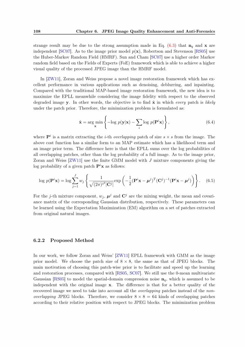
108 Chapter 6. JPEG Image Quality Enhancement and Anti-Forensics
strange result may be due to the strong assumption made in Eq. (6.3) that nq and x areindependent [SC07]. As to the image prior model p(x), Robertson and Stevenson [RS05] usethe Huber-Markov Random Field (HMRF). Sun and Cham [SC07] use a higher order Markovrandom field based on the Fields of Experts (FoE) framework which is able to achieve a highervisual quality of the processed JPEG image than the HMRF model.
In [ZW11], Zoran and Weiss propose a novel image restoration framework which has ex-cellent performance in various applications such as denoising, deblurring, and inpainting.Compared with the traditional MAP-based image restoration framework, the new idea is tomaximize the EPLL meanwhile considering the image fidelity with respect to the observeddegraded image y. In other words, the objective is to find x in which every patch is likely
under the patch prior. Therefore, the minimization problem is formulated as:
x = arg minx
{
−log p(y|x)−∑
i
log p(Pix)
}
, (6.4)
where Pi is a matrix extracting the i-th overlapping patch of size s× s from the image. Theabove cost function has a similar form to an MAP estimate which has a likelihood term andan image prior term. The difference here is that the EPLL sums over the log probabilities ofall overlapping patches, other than the log probability of a full image. As to the image prior,Zoran and Weiss [ZW11] use the finite GMM model with J mixture components giving thelog probability of a given patch Pix as follows:
log p(Pix) = logJ∑
j=1
wj
{
1√
(2π)s2 |Cj |exp
(
−1
2(Pix− µj)T (Cj)−1(Pix− µj)
)
}
. (6.5)
For the j-th mixture component, wj , µj and Cj are the mixing weight, the mean and covari-ance matrix of the corresponding Gaussian distribution, respectively. These parameters canbe learned using the Expectation Maximization (EM) algorithm on a set of patches extractedfrom original natural images.
6.2.2 Proposed Method
In our work, we follow Zoran and Weiss’ [ZW11] EPLL framework with GMM as the imageprior model. We choose the patch size of 8 × 8, the same as that of JPEG blocks. Themain motivation of choosing this patch-wise prior is to facilitate and speed up the learningand restoration processes, compared with [RS05, SC07]. We still use the 0-mean multivariateGaussian [RS05] to model the spatial-domain compression noise nq, which is assumed to beindependent with the original image x. The difference is that for a better quality of therecovered image we need to take into account all the overlapping patches instead of the non-
overlapping JPEG blocks. Therefore, we consider 8 × 8 = 64 kinds of overlapping patchesaccording to their relative position with respect to JPEG blocks. The minimization problem

6.2. JPEG Image Quality Enhancement 109
is then formulated as:
x = arg minu
64∑
k=1
∑
Pi∈Sk
1
2
(
Pi(y − u))t(Ck)−1Pi(y − u)−
∑
i
log p(Piu)
, (6.6)
where Sk is the k-th set of matrices which extract patches having the same relative positionswith respect to JPEG blocks, and Ck is the covariance matrix for modeling the compressionnoise of the k-th group of patches. Besides, log p(Piu) is derived by replacing Pix in Eq. (6.5)by Piu. The optimization of Eq. (6.6) can be solved using an approximate MAP estimationprocedure giving a Wiener filter solution (for more details, please refer to [ZW11]). At last,a QCS projection is used to assure that the DCT coefficient of the processed image is withinthe same quantization bin as that of the JPEG image. If a DCT coefficient goes outside itsoriginal quantization bin, it will be modified to the boundary value of the quantization bin.
Practically, we learn a GMM prior with 200 mixture components from 338 × 6000 =
2028000 randomly sampled 8 × 8 patches on UCIDLearn dataset (see Section 2.3.1 for moredescriptions about the datasets). For JPEG blocks, Robertson and Stevenson [RS05] proposeto calculate the covariance matrix Cq (i.e., one of the Ck in Eq. (6.6)) from the quantizationtable Q. Sun and Cham [SC07] also experimentally prove its superiority over the actualcompression noise covariance matrix. In the proposed optimization problem in Eq. (6.6),we need to consider 63 more kinds of 8 × 8 patches besides the JPEG blocks. In thesepatches, pixels across neighboring JPEG blocks are present in the same patch. Correlations ofspatial-domain compression noise across different JPEG blocks may be difficult to calculate.Therefore, for each quality factor q, we propose to learn the 64 covariance matrices Ck onUCIDLearn dataset. More specifically, given a JPEG compression quality factor q, we JPEGcompress all the images from UCIDLearn dataset, the actual compression noise is obtainedby subtracting the JPEG image by its corresponding original image. The compression noiseis thereafter used for learning the 64 covariance matrices Ck. The learning of the GMM prioras well as the covariance matrices is performed on the 338 images from UCIDLearn datasetusing the EM algorithm with unoptimized Matlab code14.
Table 6.1 lists the PSNR results for 4 classical images and 3 quantization tables Q1, Q2 andQ3, provided by [SC07], for very low bit-rate compression. The original uncompressed imageis used as the reference for calculating the PSNR values. We can see that the proposed methodis very competitive in terms of PSNR gain. In our JPEG anti-forensic work, we consider thequality factors in {50, 51, · · · , 95}, whose corresponding quantization matrices produce muchhigher bit-rate compression than Q1, Q2 and Q3 used in [SC07]. In practice, we found thatthe PSNR gain of the proposed JPEG post-processing method is slightly lower than that ofSun and Cham’s [SC07] method using these quality factors. However, the proposed methodonly requires one step of approximate MAP estimation, which is practically around ten timesfaster than [SC07] using the conjugate gradient descent. As an intermediate result of our anti-forensic JPEG image creation (to be described later), the PSNR gain is already satisfying.We denote the processed JPEG image using the proposed quality enhancement method as IJ .
14Downloaded from: http://www.mathworks.com/matlabcentral/fileexchange/26184-em-algorithm-
for-gaussian-mixture-model.

110 Chapter 6. JPEG Image Quality Enhancement and Anti-Forensics
From the figures listed in Table 6.5, we can see that IJ achieves a PSNR gain of 0.7931 dBand an SSIM gain of 0.0008 than the JPEG image J on average, on UCIDTest dataset.
Table 6.1: PSNR (using the original image as the reference) results for 4 classical testimages and 3 different quantization tables provided in [SC07]15.
JPEG image FoE-based [SC07] Proposed
Lena
Q1 30.71 31.95 32.06
Q2 30.08 31.44 31.48
Q3 27.45 28.83 28.94
Peppers
Q1 30.72 32.04 32.09
Q2 30.17 31.61 31.59
Q3 27.66 29.35 29.40
Barbara
Q1 25.95 26.65 26.94
Q2 25.60 26.31 26.56
Q3 24.05 24.86 25.00
Baboon
Q1 24.32 24.77 24.84
Q2 24.14 24.62 24.68
Q3 22.14 22.61 22.61
After the image quality enhancement processing of J , IJ has already partly recoveredthe lost information during JPEG compression, however the DCT-domain information hasnot been very well recovered. A sample DCT histogram of IJ , which still has the comb-likequantization artifacts, is shown in Figure 6.2-(b). A natural following step goes to the DCThistogram smoothing. Other than using the global Laplacian model in [Sta+10a, SL11] or thelocal Laplacian model in Chapter 5, a new, non-parametric approach based on calibration isproposed without the consideration of any statistical model in Section 6.3.
6.3 Non-Parametric DCT Histogram Smoothing
In Section 5.2.2.1, we have discussed the disadvantages of using the Laplacian distributionto model the DCT coefficients in AC subbands, which is the basic assumption of Stamm et
al.’s [Sta+10a, SL11] dithering based JPEG anti-forensic method. For natural uncompressedimages, the DCT histograms for AC components usually have a much higher peak than theLaplacian distribution. This point can also be reflected by the big kurtosis value of ACcomponents, which is often larger than 6 (kurtosis of the Laplacian distribution).
Besides, during the creation of Stamm et al.’s [Sta+10a, SL11] anti-forensic JPEG imageFJSq
, the dithering signal is generated depending on the estimated Laplacian parameter using
15Note that in this table the PSNR results of Sun and Cham’s method are slightly different from the valueslisted in [SC07]. It is because we rounded the pixel values to integers within [0, 255] before calculating thePSNR value, while in [SC07] the PSNR is computed on floating-point “pixel values”.

6.3. Non-Parametric DCT Histogram Smoothing 111
the MLE [PR99]. The dithering process is thereafter conducted by adding the signal to thequantized DCT coefficient randomly without any consideration of the local information of theimage in the spatial domain. This constitutes another disadvantage of the method that wouldlead to a poor visual quality of FJ
Sq[VTT11]. An example can be seen in Figure 6.1-(b),
comparing with -(a).
(a) J (b) FJSq
[Sta+10a, SL11]
(c) FJbq (d) FJ
c
Figure 6.1: Comparison of DCT-domain quantization noise stacked by the spatial-domainlocation and by the 64 DCT frequencies. Results are obtained from a UCID image and itsJPEG compressed version with quality factor 50. For a better visibility of the noise images,we have taken logarithm of the noise and afterwards carried out a normalization.

112 Chapter 6. JPEG Image Quality Enhancement and Anti-Forensics
In Chapter 5, the proposed perceptual DCT histogram smoothing method considers anadaptive local dithering method which combines the Laplacian distribution and the uniformdistribution. The DCT histogram mapping using the Hungarian algorithm explicitly considersthe visual quality loss due to the DCT coefficient modification. Therefore, we can see thatFbq outperforms FSq [Sta+10a, SL11] in terms of both image quality (see Table 5.4) and KLdivergence (see Table 5.2), with the original image I as the reference. Moreover, an exampleof the DCT-domain quantization noise of Fbq can be found in Figure 6.1-(c). It can be seenthat the spatial-domain local information of the image is to some extent correctly reflected inthe DCT-domain quantization noise distribution.
Both of the DCT histogram smoothing methods for generating FSq [Sta+10a, SL11] andFbq rely on a statistical model for the DCT coefficients. In this chapter, we aim to find anew, non-parametric approach to DCT histogram smoothing. We wish to be able to estimatethe DCT-domain quantization noise, from the restored JPEG image IJ . To this end, we getinspired by the so-called calibration method which was initially used in steganalysis [FGH02].
Before presenting the algorithm, we hereby provide a brief introduction of the calibrationmethod. It was introduced by Fridrich et al. [FGH02] for steganalysis purposes to estimatethe DCT histogram of the cover-image from the stego-image. It is also used by Lai and Böhme[LB11] for JPEG forensic purposes. The main idea is to break the JPEG block structure bycropping the first 4 pixels of the JPEG image both horizontally and vertically. The calibratedimage shares some DCT-domain statistical similarities with the original uncompressed image.Therefore, we expect to estimate the DCT-domain quantization noise by comparing the cal-ibrated image and its JPEG compressed version. Based on the above analysis, we proposea new, non-parametric DCT histogram smoothing method based on relaxed calibration asdescribed in Algorithm 6.1.
Algorithm 6.1 Non-parametric DCT histogram smoothing procedure.
Require: JPEG image J with quality factor q1: Recover IJ from J by solving the optimization problem in Eq. (6.6).2: Crop IJ by 1 pixel16 both horizontally and vertically to obtain Ic.3: JPEG compress Ic with quality factor q to obtain Jc.4: Subtract the DCT coefficients of Ic by those of Jc, so as to estimate the DCT quantization
noise Nq.5: Add Nq to IJ in the DCT domain, so as to create FJ
c with smoothed DCT histograms.6: return: FJ
c
An example of DCT quantization noise of FJc , which is generated by the proposed cali-
bration based DCT histogram smoothing method, can be found in Figure 6.1-(d). It can beseen that the proposed method can also to some extent reproduce the DCT-domain quantiza-tion noise which is more or less related to the local spatial-domain information of the image.On UCIDTest dataset, we compute the KL divergence value between I and FJ
Sq, and that
between I and FJc for all DCT subbands. The difference between these two KL divergence
16Here we only crop the image by 1 pixel instead of 4 pixels as in classical image calibration, it is empiricallydetermined in order to attain higher image quality for F
Jc , the output of Algorithm 6.1.

6.3. Non-Parametric DCT Histogram Smoothing 113
values is reported in Table 6.2. In Stamm et al.’s [Sta+10a, SL11] DCT histogram smoothingmethod, the subband where all the DCT coefficients are quantized to 0 is untouched. For afair comparison for FJ
Sq, these subbands were not counted in the comparison. From Table 6.2,
we can see that FJc performs consistently better than FJ
Sqin AC components. As shown in
Figure 6.1-(b) and in the beginning of this section, we analyze that the quality degradationof FJ
Sqis due to the randomness of adding dithering signal without any consideration of the
image spatial-domain information. By comparing the results shown in Table 6.5 and those inTable 5.4, we can see that not only FJ
c achieves a lower KL divergence value, but also theaverage PSNR and SSIM of FJ
c have gains of 1.91 dB and 0.0120, respectively, compared withFJSq
[Sta+10a, SL11].
Table 6.2: The difference of the KL divergence between I and FJSq
[Sta+10a, SL11], and
that between I and FJc for all 64 DCT subbands. The average difference value over all
subbands is 0.0439 with standard deviation 0.0214. For a fair comparison for FJSq
, thesubbands, whose DCT coefficients are all quantized to 0 in the JPEG image J , are notcounted. Results are obtained on UCIDTest dataset.
rc 1 2 3 4 5 6 7 8
1 -0.0060 0.0065 0.0190 0.0369 0.0549 0.0728 0.0796 0.0474
2 0.0069 0.0227 0.0324 0.0381 0.0437 0.0719 0.0564 0.0117
3 0.0289 0.0298 0.0364 0.0416 0.0526 0.0636 0.0604 0.0081
4 0.0300 0.0351 0.0399 0.0388 0.0514 0.0796 0.0579 0.0040
5 0.0436 0.0412 0.0495 0.0571 0.0573 0.0865 0.0687 0.0161
6 0.0508 0.0469 0.0575 0.0503 0.0568 0.0728 0.0564 0.0319
7 0.0806 0.0629 0.0633 0.0630 0.0585 0.0613 0.0590 0.0415
8 0.0598 0.0401 0.0314 0.0243 0.0231 0.0138 0.0140 0.0186
Besides the comparison with Stamm et al.’s dithering based DCT histogram smoothingmethod [Sta+10a, SL11], we also would like to compare the proposed calibration based DCThistogram smoothing method proposed in this section with our other perceptual DCT his-togram smoothing method proposed in Section 5.2.2 in the following17.
From Table 6.3, we can see that the JPEG quality enhancement method proposed inSection 6.2 indeed has advantages in visual quality over the processed image FJ
b using TV-based JPEG deblocking method (see Section 5.2.1). Yet, in the DCT domain, FJ
b is able torecover more information than IJ (see the KL divergence difference in Table 6.3). Comparisonof example DCT histograms can also be seen in Figures 6.2-(a) and -(b). The remaining DCT-domain quantization artifacts in FJ
b are less obvious than those in IJ .
With another step of DCT histogram smoothing considering the perceptual quality lossdue to the DCT coefficient modification (see Section 5.2.2), FJ
bq is able to achieve smoothed
DCT histogram without much visual quality sacrifice. On the other hand, though IJ has an17Our research work published in [Fan+13a] (also see Chapter 4) and in [Fan+13b] (also see this chapter)
was conducted almost in parallel. The work published in [Fan+14] (also see Chapter 5) was carried out later.The comparison presented in this chapter among the three methods is new, and not in any published papers.

114 Chapter 6. JPEG Image Quality Enhancement and Anti-Forensics
Table 6.3: The 2nd and 3rd columns respectively list the mean (µkl) and standard deviation(σkl) of the difference of the KL divergence of the DCT histogram between different images.The 4th and 5th columns report the mean (µmse) and standard deviation (σmse) of differenceof the MSE of the unnormalized DCT histogram between different image pairs. All the 64subbands are considered, no matter whether the DCT coefficients are all quantized to 0 inthe JPEG image J . The 6th and 7th columns show the PSNR and SSIM difference. Allevaluation metrics are calculated using the original image I as the reference. The anti-forensic JPEG image is expected to have low KL divergence and MSE values of the DCThistogram and high PSNR and SSIM values. Results are obtained on UCIDTest dataset.
µkl σkl µmse σmse PSNR SSIM
FJb vs. IJ -0.4368 0.1481 -17863.56 15711.74 -1.1525 -0.0036
FJbq vs. FJ
c -0.0239 0.0431 -2195.72 2686.60 0.6717 -0.0004
FJ0 vs. FJ
1 -0.0041 0.0328 584.18 980.70 0.2246 0.0011
FJ vs. FJ1 -0.0202 0.0295 -143.63 745.90 0.7287 0.0034
DCT coefficient value
DCT
coeffi
cientfrequency
−200 −100 0 100 2000
0.05
0.10
0.15
0.20
0.25
(a) FJb
DCT coefficient value
DCT
coeffi
cientfrequency
−200 −100 0 100 2000
0.05
0.10
0.15
0.20
0.25
(b) IJ
DCT coefficient value
DCT
coeffi
cientfrequency
−200 −100 0 100 2000
0.02
0.04
0.06
(c) FJbq
DCT coefficient value
DCT
coeffi
cientfrequency
−200 −100 0 100 2000
0.05
0.10
0.15
0.20
(d) FJc
Figure 6.2: Example (2, 2) subband DCT histograms of FJb , IJ , FJ
bq and FJc . The corre-
sponding JPEG image J is compressed with quality factor 50 from a UCID image.

6.3. Non-Parametric DCT Histogram Smoothing 115
even higher visual quality than the JPEG image J , extra noise is later introduced in FJc , by
adding the estimated DCT-domain quantization noise estimated based on calibration directlyback to IJ . This results in that FJ
c achieves a lower image quality than FJbq. On the DCT
histogram recovery side, FJbq is able to achieve a lower KL divergence value than FJ
c on average
over all 64 DCT subbands. However, Table 6.4 shows that in fact FJc performs better than
FJbq in the low-frequency DCT subbands. Though FJ
c does not outperform FJbq in general, we
can conclude that the very simple slight cropping helps Ic get a quite good estimation of theoriginal DCT histogram of I, especially in the low-frequency DCT subbands.
Table 6.4: The difference of the KL divergence between I and FJbq, and that between I and
FJc for all 64 DCT subbands. The average difference value over all subbands is -0.0239 with
standard deviation 0.0431. All the subbands are considered, no matter whether the DCTcoefficients are all quantized to 0 in the JPEG image J . Results are obtained on UCIDTestdataset.
rc 1 2 3 4 5 6 7 8
1 -0.0081 -0.0001 0.0096 0.0121 0.0075 0.0126 0.0171 -0.0265
2 0.0037 0.0081 0.0127 0.0025 -0.0013 0.0201 0.0056 -0.0393
3 0.0171 0.0120 0.0098 -0.0036 -0.0062 -0.0050 -0.0099 -0.0663
4 0.0133 0.0046 -0.0013 -0.0110 -0.0194 -0.0086 -0.0097 -0.0708
5 0.0106 0.0022 -0.0037 -0.0159 -0.0291 -0.0237 -0.0591 -0.1173
6 0.0090 0.0114 -0.0104 -0.0179 -0.0323 -0.0253 -0.0692 -0.1229
7 0.0353 0.0223 -0.0124 -0.0079 -0.0660 -0.0690 -0.0936 -0.1067
8 -0.0050 -0.0332 -0.0730 -0.0720 -0.1385 -0.1372 -0.1235 -0.0357
In all, the perceptual DCT histogram smoothing after TV-based JPEG deblocking pro-posed in Section 5.2.2 outperforms the proposed calibration based DCT histogram smoothingmethod proposed in this section, in both overall DCT histogram recovery and visual qualityof the processed image. However, also as discussed in Section 5.3.3, the perceptual DCThistogram smoothing method proposed in Section 5.2.2 is the bottleneck of the computationcost of the proposed JPEG anti-forensic method in Chapter 5. As to the calibration basedDCT histogram smoothing method, it is much less computationally demanding for cropping,JPEG compression and computing/adding the DCT-domain quantization noise.
Furthermore, some possible improvements over the method proposed in this section are asfollows. In order to decrease the KL divergence values in the high-frequency DCT subbandsfor FJ
c , we could conduct a “clever cropping” for the calibration. For example, the quantizationnoise of different subbands can be estimated by cropping different “optimal” numbers of pixelsin the calibration. Moreover, the image quality of FJ
c could also be improved by conductinga similar procedure to the DCT mapping described in Section 5.2.2.3 in the perceptual DCThistogram smoothing method. A hybrid method combining the calibration based and theperceptual DCT histogram smoothing methods is likely to further push the performance ofJPEG anti-forensics towards a better DCT histogram recovery as well as a higher image qualityof the anti-forensic JPEG image, compared with the proposed methods in this thesis.

116 Chapter 6. JPEG Image Quality Enhancement and Anti-Forensics
6.4 Proposed JPEG Anti-Forensics
As analyzed in Section 6.3, we are aware that the DCT-domain quantization noise estimationbased on calibration cannot be very accurate. The injection of Nq must have introduced someextra unnatural spatial-domain noise to IJ . In this section, we will focus on the denoising onFJc as well as JPEG anti-forensics against the detectors. For convenience, the spatial-domain
noise present in FJc is assumed to be additive white Gaussian noise, with standard deviation
σn. The forensic detectors in consideration are KF [FD03], KV [Val+11] and KL [LB11]18.
We still follow Zoran and Weiss’ [ZW11] EPLL based image restoration framework, yetadding some terms for JPEG anti-forensic purposes. The minimization problem we proposeto solve is formulated as follows:
x = arg minu
{
λ
2‖u− y‖2 + α× ι(u) + β
28∑
k=1
7∑
c=0
∣
∣νk(uc)− σ2k∣
∣+∑
i
γ
2‖Piu− zi‖2
−log p(zi)
}
, (6.7)
where λ, α, β and γ are regularization parameters, uc is the calibrated image obtained bycropping u by c pixels in both horizontal and vertical directions [FGH02, LB11], and {zi} isa set of auxiliary variables facilitating the optimization [ZW11].
Now we explain the different terms in Eq. (6.7) in order. The first term is for the imagefidelity control, which expects the obtained image is still close to the given JPEG image. Thesecond term is designed for KV [Val+11], and ι(·) computes the TV of the image (the ℓ1 normof the spatial first-order derivatives). We wish the image would have low TV, in other wordsnot very noisy. The third term is for KL [LB11], and νk(·) returns the variance of the k-thhigh-frequency subband (defined in [LB11]) of the image, while σ2k is the estimated varianceof the original image from the k-th high-frequency DCT subband of FJ
c . As the JPEG blocksize is 8 × 8, basically we have 7 ways to crop the image along the diagonal direction by c
(c = 1, · · · , 7) pixel(s) in both horizontal and vertical directions. Following the main ideaof KL, 6 other detectors can be built using the similar way by comparing the variances ofhigh-frequency subbands between the image and its calibrated version. If the image and allits 7 calibrated versions have close variances to the estimated one in all the high-frequencysubbands, KL and the other 6 potential detectors described above can be fooled. The lastterm is the image prior term which expects every patch is likely under the prior, because of
18The JPEG anti-forensic method presented in this chapter was published in a conference paper [Fan+13b]in 2013. At that time, in literature KF , KV and KL are the scalar-based forensic detectors specificallyconsidered in the state-of-the-art JPEG anti-forensics [Sta+10a, Sta+10b, SL11] and forensics [Val+11, LB11]to counter JPEG anti-forensics. We think it is possible to integrate more anti-forensic terms into the costfunction in Eq. (6.7) to further improve the forensic undetectability of the anti-forensic JPEG image againstmore detectors. We will leave it as a future study. Different from [Fan+13b], in this section, we test theanti-forensic JPEG image against all the 8 scalar-based JPEG forensic detectors listed in Table 3.1, thoughsome of them were not considered in [Fan+13b]. The test of the proposed anti-forensic JPEG image in thischapter against the two SVM-based detectors used in Chapter 5 and some possible improvement will also beleft as a future work.

6.4. Proposed JPEG Anti-Forensics 117
which the outputs of KF [FD03] can be largely decreased.
The optimization problem can be solved using the “Half Quadratic Splitting” [ZW11] (seeSection 2.4.3 for more details) and it consists of two sub-problems:
• z sub-problem, solving z given u — This is solved using the approximate MAP estima-tion, given the parameter γ which is related to the noise standard deviation σn [ZW11].The main objective of this sub-problem is to remove the introduced extra unnaturalnoise in FJ
c , through the regularization by the natural image statistical model.
• u sub-problem, solving u given z — This can be solved using the subgradient method(see Section 2.4.1 for more details). JPEG anti-forensics is mainly carried out in thissub-problem, while keeping the image still close to y.
For solving Eq. (6.7), we do 3 iterations and the parameter setting is: λ = s2
10σ2n, α = s2
10σ2n,
β = 8s2
10σ2n, γ = 1
σ2n[1, 8, 32], and σn is empirically set as−0.1q+13 according to the quality factor
q of J . For each iteration of constant γ value, z and x sub-problems are solved alternativelyonce for either problem. In practice, we found that the output of KL [LB11] is not easy to befurther decreased into the normal range. Moreover, images tend to be over-smoothed as KQ
F
[FD03] detects many ‘3’ entries (see Section 4.2.1 for more explanation and analysis on this).We tackle this problem by adding a slight amount of white Gaussian noise in the middle ofsolving the x sub-problem during the last iteration. We set λ = 0, α = 0.01 and β = 1 toemphasize on decreasing the KL output. The added noise is mostly suppressed during the latersubgradient iterations but can successfully reduce the occurrences of ‘3’ in the quantizationtable estimation of KQ
F [FD03].
False positive rate
Truepositiverate
0 0.2 0.4 0.6 0.8 10
0.2
0.4
0.6
0.8
1
KF
KLuo
KQLuo
KV
KL
K1U
K2U
Random guess
Figure 6.3: ROC curves achieved by FJ1 against scalar-based JPEG forensic detectors.
Results are obtained on UCIDTest dataset.

118 Chapter 6. JPEG Image Quality Enhancement and Anti-Forensics
Table 6.5: From the 2nd to the 8th columns, the AUC values for different kinds of imagesagainst scalar-based JPEG forensic detectors are listed; the image quality (with I as thereference) comparison is reported in the last 2 columns. Results are obtained on UCIDTestdataset.
KF KLuo KQLuo KV KL K1
U K2U PSNR SSIM
J 0.9991 1.0000 0.9996 0.9976 0.9811 0.9860 0.8840 37.0999 0.9919
FJSqSb
0.3783 0.0806 0.6288 0.8337 0.5338 0.6309 0.4854 30.4591 0.9509
IJ 0.9997 0.9982 0.9528 0.7851 0.9698 0.9878 0.8779 37.8930 0.9927
FJc 0.9994 0.8147 0.5949 0.7383 0.9868 0.9868 0.8944 35.3209 0.9876
FJ1 0.5522 0.7291 0.3594 0.739419 0.5272 0.7750 0.5787 35.2568 0.9832
FJ0 0.6756 0.6046 0.5194 0.6210 0.4490 0.6772 0.5880 35.4814 0.9843
FJ 0.5398 0.6425 0.4598 0.6159 0.4344 0.5894 0.5317 35.9855 0.9866
Let FJ1 denote the anti-forensic image created using the proposed method described in
this chapter. Figure 6.3 shows the ROC curves of FJ1 against 7 scalar-based JPEG forensic
detectors listed in Table 3.1. Table 6.5 reports the AUC values and average PSNR and SSIMvalues of different (anti-forensic/post-processed) JPEG images. We also calculated the AUCvalues of FJ
1 against the above mentioned 6 potential detectors which are built in a similarway as KL [LB11], the average AUC value is 0.4456 with the standard deviation 0.0872.Compared with the state-of-the-art anti-forensic JPEG images [Sta+10a, Sta+10b, SL11,VTT11, SS11] (see Table 5.4 for AUC, PSNR and SSIM values, and see Figures 4.2 for ROCcurves), our anti-forensic JPEG image FJ
1 achieves a better tradeoff between undetectabilityagainst existing JPEG forensic detectors and the visual quality of processed images. Take thecomparison with FSqSb
[Sta+10a, Sta+10b, SL11] as an example, not only a slightly betteroverall forensic undetectability is achieved, but also FJ
1 has a PSNR gain of 4.80 dB and anSSIM gain of 0.0323.
Figure 6.4 shows example results of (anti-forensic) JPEG images compared with the origi-nal image. As demonstrated in Figure 6.4-(d), FJ
1 is able to keep more details such as texturesand edges than FSqSb
[Sta+10a, Sta+10b, SL11] exampled in -(c) (please refer to the elec-tronic version for a better visibility). Even though the quantization table estimation baseddetector KQ
F [FD03] was proven not very reliable in Section 4.2.1, we still tested it on FJ1 on
UCIDTest dataset. Among all the anti-forensic JPEG images, 94.50% of them are classifiedas never compressed by KQ
F . We also examine the shape of the DCT histogram, and someexample results are shown in Figure 6.5, in which no noticeable artifacts can be observed.
The last two rows of Table 6.3 show the DCT histogram recovery and image qualitycomparison of FJ
1 , FJ0 , and FJ . It can be seen that both FJ
0 and FJ outperform FJ1 .
19In our published paper [Fan+13b], the KV detector is another version presented in Valenzise et al.’s work[Val+11], other than the version (in Valenzise et al.’s improved work in [VTT13]) used in this thesis. In thatsetting, there is a lag parameter (see [Val+11] for details) set as 5 for the re-compression quality factors for KV .This specific setting is for the consideration that the quality factors in use in [Fan+13b] are integer multiplesof 5. These setting changes result in the relatively high AUC value shown here for F
J1 against KV [VTT13].

6.4. Proposed JPEG Anti-Forensics 119
(a) I (b) J
(c) FSqSb(d) FJ
1
Figure 6.4: Example results (close-up images) of FJ1 compared with I, J , and FSqSb
[Sta+10a, Sta+10b, SL11], where J is compressed with quality factor 50.
However, we know that the DCT histogram is not well smoothed in FJ0 (an example can be
seen in Figure 4.10-(b)). Yet, its average KL divergence has an even lower value than thatof FJ
1 whose DCT histogram is explicitly smoothed by the proposed calibration based DCThistogram smoothing method described in Section 6.3. This may be explained by the factthat the smoothness of the DCT histogram is not always conveyed by the KL divergence.Therefore, we also calculate the MSE (see Eq. (2.5) for the version on images, the calculationon histograms is similar) between the unnormalized DCT histogram of the processed JPEGimage and that of its corresponding original image. The mean and standard deviation of thedifference of these MSE values are reported in the 4th and the 5th columns of Table 6.3. Underthis evaluation metric, FJ
1 outperforms FJ0 .
Generally speaking, compared with FJ0 generated by our JPEG anti-forensic method in
Chapter 4 and FJ generated by our JPEG anti-forensic method in Chapter 5, the anti-forensicJPEG image FJ
1 created in this chapter does not outperform them in terms of forensic unde-tectability and visual quality of the processed image (see Tables 6.3 and 6.5 for the comparison,

120 Chapter 6. JPEG Image Quality Enhancement and Anti-Forensics
DCT coefficient value
DCT
coeffi
cientfrequen
cy
−200 −100 0 100 2000
0.04
0.08
0.12
0.16
(a) (2, 2)
DCT coefficient value
DCT
coeffi
cientfrequency
−100 −50 0 50 1000
0.1
0.2
0.3
(b) (1, 6)
DCT coefficient value
DCT
coeffi
cientfrequency
−30 −20 −10 0 10 20 300
0.1
0.2
0.3
(c) (7, 4)
DCT coefficient value
DCT
coeffi
cientfrequency
−10 −5 0 5 100
0.2
0.4
0.6
(d) (8, 8)
Figure 6.5: Example DCT histograms of different subbands of an anti-forensic JPEG imageFJ
1 shown in Figure 6.4-(d). No noticeable comb-like DCT quantization artifacts appear inthe histograms.
ROC curves can also be compared in Figure 4.6-(c), Figure 5.8-(b) and Figure 6.3). Intuitively,this is to some extent out of our expectation. We expected that the more sophisticated imageprior model would be able to push the performance of the resulting anti-forensic JPEG imagetowards a higher image quality than the TV-based method while still keeping a good foren-sic undetectability. However, these results are understandable and may be explained by thefollowing reasons:
• In fact, the ability of the EPLL framework with the GMM as the image prior for JPEGimage quality enhancement is proven by experiments on 4 classical test images (seeTable 6.1) and a large-scale test on UCIDTest dataset (see Table 6.5). However, as shownin Figure 6.2-(b) compared with -(a) produced by the TV-based JPEG deblocking, theDCT coefficient modification in IJ is relatively minor. In order to remove the remainingcomb-like DCT-domain quantization artifacts, the cost will be more expensive. In otherwords, more image quality may need to be sacrificed. On the other hand, IJ is our only
6.5. Summary 121
kind of (intermediate) anti-forensic JPEG image in this thesis that has a higher visualquality than the JPEG image. Further improvement would be possible to create fromIJ the anti-forensic JPEG image with even higher quality than the JPEG image, if thefollowing anti-forensic steps are more carefully designed.
• As shown in Figure 6.1-(d), the calibration is able to help IJ get a quite good estimationof the DCT-domain quantization noise with some spatial-domain coherence. The processis very fast, however the estimation is still quite crude. This leads to main imagedegradation (see the PSNR value change from the 4nd row to the 5th row in Table 6.5)during the creation of the proposed anti-forensic JPEG image FJ
1 .
• Regarding the forensic undetectability, FJ1 has less good anti-forensic performance in
blocking artifacts or spatial-domain unnatural noise examination than FJ0 and FJ . This
may be explained by the fact that there is an explicit TV-based deblocking term (seeEq. (4.6) and Figure 4.3) in the creation of FJ
0 and FJ , which is not used in Eq. (6.7).
6.5 Summary
By using the MAP-based image restoration, calibration and a prior of natural image statistics,we create anti-forensic JPEG image FJ
1 which outperforms the state-of-the-art anti-forensicJPEG images [Sta+10a, Sta+10b, SL11, VTT11, SS11] with a higher image quality as well as aslightly better forensic undetectability against existing forensic detectors. Moreover, the DCThistogram is explicitly smoothed by the proposed calibration based DCT-domain quantizationnoise estimation to better approximate the original one.
However, the proposed method based on a sophisticated image prior model does not out-perform our previous JPEG anti-forensic methods proposed in Chapters 4 and 5. The possiblereasons are provided in the end of Section 6.4. As a preliminary JPEG anti-forensics workleveraging on more sophisticated image prior model than the TV, the performance of theproposed method in this chapter may be further improved by a more accurate DCT-domainquantization noise estimation and the integration of more anti-forensic terms in Eq. (6.7).Some ideas of possible improvement are provided at the end of Sections 6.3 and 6.4. Oneambitious but challenging objective is to create anti-forensic JPEG images with even highervisual quality than the JPEG image, where a good image prior model would be indispensable.
From Chapter 4, Chapter 5 and this chapter, we have seen the superiority of anti-forensicmethods designed based on concepts/methods from image restoration over the methods basedon noise injection and simple image processing. This draws our interest to work on otherimage anti-forensic problems following the same research line. During our study of JPEG anti-forensics, we are aware that Stamm et al. [Sta+10b, SL11] propose to use median filtering toremove the spatial-domain blocking artifacts from a JPEG image. Moreover, median filtering isalso used for image resampling anti-forensic purposes in [KR08]. The median filtering tracespresent in one image, not only expose that the image is median filtered, but also indicateother image processing operations may have been applied. Therefore, it is important to study

122 Chapter 6. JPEG Image Quality Enhancement and Anti-Forensics
median filtering on the anti-forensic side. This work will be conducted in Chapter 7, by stillfollowing our research line of leveraging on image restoration to design image anti-forensics.

Chapter 7
Median Filtered Image Quality
Enhancement and Anti-Forensics via
Variational Deconvolution
Contents7.1 Introduction and Motivation . . . . . . . . . . . . . . . . . . . . . . . . . 125
7.2 Analysis of Median Filtering and Its Impact on Image Statistics . . . 126
7.2.1 Median Filtering Process . . . . . . . . . . . . . . . . . . . . . . . . . . . 126
7.2.2 Observations of Pixel Value Difference Distribution . . . . . . . . . . . . . 127
7.3 Proposed Image Variational Deconvolution Framework . . . . . . . . 129
7.3.1 Problem Formulation . . . . . . . . . . . . . . . . . . . . . . . . . . . . . 129
7.3.2 Kernel Selection and Parameter Settings . . . . . . . . . . . . . . . . . . . 132
7.3.3 Median Filtered Image Quality Enhancement . . . . . . . . . . . . . . . . 133
7.3.4 Anti-Forensics against Median Filtering Detection . . . . . . . . . . . . . 135
7.3.4.1 Pixel Value Perturbation . . . . . . . . . . . . . . . . . . . . . . 137
7.3.4.2 Parameter Settings . . . . . . . . . . . . . . . . . . . . . . . . . 138
7.3.4.3 Performance Evaluation and Comparison . . . . . . . . . . . . . 142
7.4 Applications: Disguising Footprints of Both Median Filtering andTargeted Image Operation of Median Filtering Processing . . . . . . 146
7.4.1 Hiding Traces of Image Resampling . . . . . . . . . . . . . . . . . . . . . 146
7.4.2 Removing JPEG Blocking Artifacts . . . . . . . . . . . . . . . . . . . . . 149
7.5 Summary . . . . . . . . . . . . . . . . . . . . . . . . . . . . . . . . . . . . 150
This chapter proposes an image variational deconvolution framework for both quality en-hancement and anti-forensics of the median filtered image (i.e., MF image for short).
The proposed optimization-based framework consists of a convolution term, a fidelity termwith respect to the MF image, and a prior term. The first term is for the approximation ofthe median filtering process, using a convolution kernel. The second fidelity term keeps theprocessed image to some extent still close to the MF image, retaining some denoising or otherimage processing artifacts hiding effects. Using the generalized Gaussian as the distributionmodel, the last image prior term regularizes the pixel value derivative of the obtained imageso that its distribution resembles that of the original image. The proposed method can serveas an MF image quality enhancement technique, whose efficacy is validated by experimentsconducted on MF images which have been previously “salt & pepper” noised. Using anotherparameter setting and with an additional pixel value perturbation procedure, the proposed
123

124 Chapter 7. Median Filtered Image Quality Enhancement and Anti-Forensics
method outperforms the state-of-the-art median filtering anti-forensic methods, with a bet-ter forensic undetectability against existing detectors as well as a higher visual quality ofthe processed image. Furthermore, the feasibility of concealing image resampling traces andJPEG blocking artifacts is demonstrated by experiments, using the proposed median filteringanti-forensic method.
A paper describing this work has been accepted for publication in an international journal[Fan+15]. The Matlab code of the method is freely shared online and can be downloaded from:http://www.gipsa-lab.grenoble-inp.fr/~wei.fan/documents/AFMF-TIFS15.tar.gz.

7.1. Introduction and Motivation 125
7.1 Introduction and Motivation
In Chapters 4, 5 and 6, we have seen the feasibility of employing some concepts/methods fromimage restoration meanwhile integrating some extra anti-forensic terms/strategies to deviseJPEG anti-forensics with better performance than the state-of-the-art methods. In this chap-ter, we still follow this research line and study another image anti-forensic problem, that is,median filtering anti-forensics. Our choice to study median filtering is because of its link toJPEG anti-forensics, which is one of our two main research topics in this thesis. In [Sta+10b,SL11], Stamm et al.’s proposed to use median filtering for removing the JPEG blocking ar-tifacts in the spatial domain after the DCT histogram of the JPEG image is smoothed by adithering operation [Sta+10a, SL11]. Despite of the effectiveness of median filtering in theJPEG blocking artifacts removing task, the resulting anti-forensic JPEG image has not beenexamined by median filtering forensic detectors yet [BK13]. This partially motivates us toconduct the study of median filtering anti-forensics.
The median filter, a well-known local image operator, is frequently adopted for image de-noising or smoothing purposes. Median filtering has the reputation of good edge preservingability, and does not introduce new pixel values to the processed image. However, median fil-tering also has the shortcoming to degrade the image quality, causing undesired image blurring.Besides, image anti-forensic researchers pointed out the destructive nature of median filteringto other image processing footprints, e.g., disguising JPEG blocking artifacts [Sta+10b, SL11]as described earlier, and hiding traces of image resampling [KR08]. Therefore, the presence ofmedian filtering traces, not only suggests the image has been previously median filtered, butalso implies the possibility that other image processing operations may have been applied tothe image.
Similar to our JPEG anti-forensic work presented in Chapter 6, we would like to firstconsider image restoration of MF images, via solving an ill-posed inverse problem. Morespecifically, the specific inverse problem of median filtering can be treated as a blind decon-volution problem. The word “blind ” means that we do not have complete knowledge aboutthe convolution kernel used for the filtering. In general, for image deconvolution, the MAPestimation (or one of its variants) is often employed. For the non-blind deconvolution problem,the convolution kernel is known and the use of a good image prior is essential for the problemsolving [KF09, KTF11]. As to the blind deconvolution, it is a popular way to perform thekernel estimation first and thereafter solve the problem using non-blind methods [Lev+09,KTF11]. Yet, the median filtering deconvolution is an even more difficult task, since the ker-nel is not only unknown but also spatially heterogeneous. As a first trial to solve this difficultproblem, in this chapter we simplify it to be a tractable blind deconvolution problem with anapproximated spatially homogeneous kernel.
In this chapter, we investigate into the median filtering process and the pixel value differ-ence statistical change caused by median filtering. Thereafter, we choose a proper convolutionkernel by experimentally studying several spatially homogeneous convolution kernels. As tothe image prior, we use the generalized Gaussian distribution to model the pixel value dif-ference whose statistics have a notable change after the image is median filtered. By using a

126 Chapter 7. Median Filtered Image Quality Enhancement and Anti-Forensics
proper convolution kernel and a good image prior, we form an image variational devolutionframework to solve the inverse problem of median filtering. The achievement of the proposedframework is two-fold: (i) improving the visual quality of MF images (with a certain parame-ter setting) as an image quality enhancement method, and (ii) fooling existing median filteringforensic detectors (with another parameter setting and an additional pixel value perturbationprocedure) for anti-forensic purposes.
The remainder of the thesis is organized as follows. Section 7.2 analyzes the median filteringprocess and image derivative statistical change due to median filtering. The proposed methodis described in Section 7.3, where experimental results of MF image quality enhancementand anti-forensics are also presented, with comparisons with the state-of-the-art anti-forensicmethods. In Section 7.4, the proposed median filtering anti-forensic method is proven to bepractical in the application of image resampling and JPEG blocking anti-forensics, again withexperimental comparisons with the state-of-the-art methods. Finally, a summary is given inSection 7.5.
7.2 Analysis of Median Filtering and Its Impact on ImageStatistics
7.2.1 Median Filtering Process
According to Eq. (3.11) (basics of median filtering can be found in Section 3.2.1), for eachlocal window, the median filter outputs the median value inside the filter window. During themedian filtering process, no new pixel values are generated. For the considered 3× 3 window,and for each local window, the median filter can be expressed using a 3× 3 convolution kernelmatrix:
Ψk =
ψk1 ψk
4 ψk7
ψk2 ψk
5 ψk8
ψk3 ψk
6 ψk9
,with ψk
k = 1 and ψki = 0 for ∀i 6= k,
i, k ∈ {1, 2, · · · , 9}, (7.1)
which can come in 9 shapes. Nevertheless, for a specific pixel neighborhood, the form of Ψk
in use is completely dependent on the order statistics of the original pixels compassed by thefilter window. Yet, this piece of information is permanently lost during the median filteringprocess.
Median filtering is a spatially heterogeneous process. For each pixel xi of the originalimage x, there are s2 possible masks (i.e., the convolution kernel matrices in Eq. (7.1)) inchoose, during the median filtering process. For an N -pixel image, the space of possible maskcombinations is enormous – there are (s2)N possibilities (with a small window size 3×3, and avery small image with size 10×10, there are 2.7×1095 possibilities). It appears not practical toconsider all the (s2)N possible mask combinations for modeling the median filtering process. Inorder to simplify this model, we propose, as a first trial, to use a single mask and approximate
the median filtering process as a spatially homogeneous image convolution procedure. A keyissue here concerns a properly defined convolution kernel, and we postpone the relevant study

7.2. Analysis of Median Filtering and Its Impact on Image Statistics 127
and discussion to Section 7.3.2, where 6 different kinds of spatially homogeneous kernels areexperimentally compared.
Based on the above analysis, Section 7.3.1 will further formulate the median filteringprocess approximation as the first term in Eq. (7.4). Indeed, the modeling may appear to beoversimplified, which however makes the problem easy to solve and in practice yields goodresults (see Sections 7.3.3 and 7.3.4). It is an interesting yet difficult open research problemto estimate the spatially heterogeneous convolution kernel for median filtering, and we leaveit for a future study.
7.2.2 Observations of Pixel Value Difference Distribution
Kirchner and Fridrich [KF10] built the forensic measures KK and KK (see Eqs. (3.12)-(3.13)in Section 3.2.2) based on the first-order pixel value difference histogram. The SPAM feature[PBF10] is based on the analysis of the first-order pixel value difference images, and was ini-tially designed for measuring the effects of ±1 steganography. It also performed excellentlyin distinguishing MF images from the original [KF10]. The feature proposed by Cao et al.
[Cao+10] was built by measuring the first-order pixel value difference image in the texturedareas. Yuan [Yua11] did not directly use the pixel value difference for constructing the feature.However, the MFF feature measures local pixel dependency artifacts, where the pixel valuedifference statistics can contribute as an important one. Also, Chen et al. [CN11] studied thepixel neighbor correlation, using a linear prediction model. Furthermore, in [Che+12, CNH13],Chen et al. explicitly pointed out that their median filtering forensic method works in theimage pixel value difference domain. Kang et al. [PK12, Kan+12, Kan+13] did not work onthe image pixel value difference domain directly, but on the median filter residual. Neverthe-less, they studied the residual correlation in a certain neighborhood, using the Markov chains[PK12] or the autoregressive model [Kan+12, Kan+13]. Concerning Zhang et al.’s [Zha+14]median filtering discriminating feature, it was built on the first-order image derivatives.
From the above analysis, we can see that existing median filtering forensic methods [KF10,PBF10, Cao+10, Yua11, CN11, Che+12, CNH13, PK12, Kan+12, Kan+13, Zha+14] eitherdirectly analyze the pixel value difference of the image, or study the image statistical changeafter median filtering in a highly related way. This motivates us to conduct study in thepixel value difference domain as well, via constructing histograms. More precisely, given animage u, we convolve it using a derivative filter, e.g., the first-order horizontal one f1 =
[1,−1] to obtain the pixel value difference, and then construct its histogram with integers{−255,−254, · · · , 255} as bin centers. For the sake of brevity, we use the matrix multiplicationF1u to denote the pixel value difference extraction from the image u using the filter f1. Thefirst-order horizontal pixel value difference histogram of an example MFTE (see Section 2.3.2for the datasets we use for median filtered image quality enhancement and forensic testing)image is shown in Figure 7.1-(a).
In order to properly model the pixel value difference, we adopt the 0-mean two-parametergeneralized Gaussian distribution, which enjoys its popularity in natural image statistics

128 Chapter 7. Median Filtered Image Quality Enhancement and Anti-Forensics
Pixel value difference
Frequency
−300 −100 100 3000
0.1
0.2
0.3
Observed dataFitted p.m.f. curve
(a) Original image
Pixel value difference
Frequency
−300 −100 100 3000
0.1
0.2
0.3
Observed data
(b) MF image
Figure 7.1: First-order horizontal pixel value difference histograms of an example MFTEimage and its MF version. The sample variance and sample kurtosis of the pixel valuedifferences are respectively: (a), σ2 = 36.2568, κ = 27.4651; (b), σ2 = 29.8866, κ = 36.6555.The red curve in (a) is its fitted p.m.f. curve, using the generalized Gaussian distribution
with estimated parameters α = 0.4797, and β = 0.4860. The squared fitting error is 0.0047.
[BS99, WSL13]. Its p.d.f. of random variable d is given by:
g(d) =β
2αΓ(1/β)e−(|d|/α)β , (7.2)
where α (> 0) is the scale parameter, β (> 0) is the shape parameter, and Γ(·) is the Gammafunction. The two parameters α and β are directly related to the variance and the kurtosis ofthe distribution:
σ2 =α2Γ(3/β)
Γ(1/β), κ =
Γ(5/β)Γ(1/β)
Γ(3/β)2. (7.3)
Therefore, the estimated parameters α and β can be obtained from the sample variance andkurtosis, by solving the above two equations, using a numerical method [BS99].
The red curve in Figure 7.1-(a) shows the fitted p.m.f. for the pixel value differencehistogram, which well describes its shape. The average squared fitting error on MFTE datasetis 0.0107, which also indicates that the generalized Gaussian distribution is a good model interms of goodness-of-fit. As a counterpart of Figure 7.1-(a), -(b) presents the first-orderhorizontal pixel value difference histogram for the median filtered version of the exampleoriginal MFTE image. We also calculate the average variance and kurtosis of the p.m.f. ofF1u on MFTE dataset, for the original images and the MF images, respectively. For F1x, theaverage variance is 129.2823, and the average kurtosis is 22.8263. Whereas for MF images,the average variance of F1y is 80.5936 and its average kurtosis is 40.0911, which are notablylower and higher than those of the original images, respectively. Indeed, the median filter isknown to have image smoothing effects, leading to (nearly) constant pixel values in a certainneighborhood. This will lead to a remarkably high peak at bin 0 of the derivative histogramafter median filtering, e.g., Figure 7.1-(b), which is embodied by the high kurtosis and low
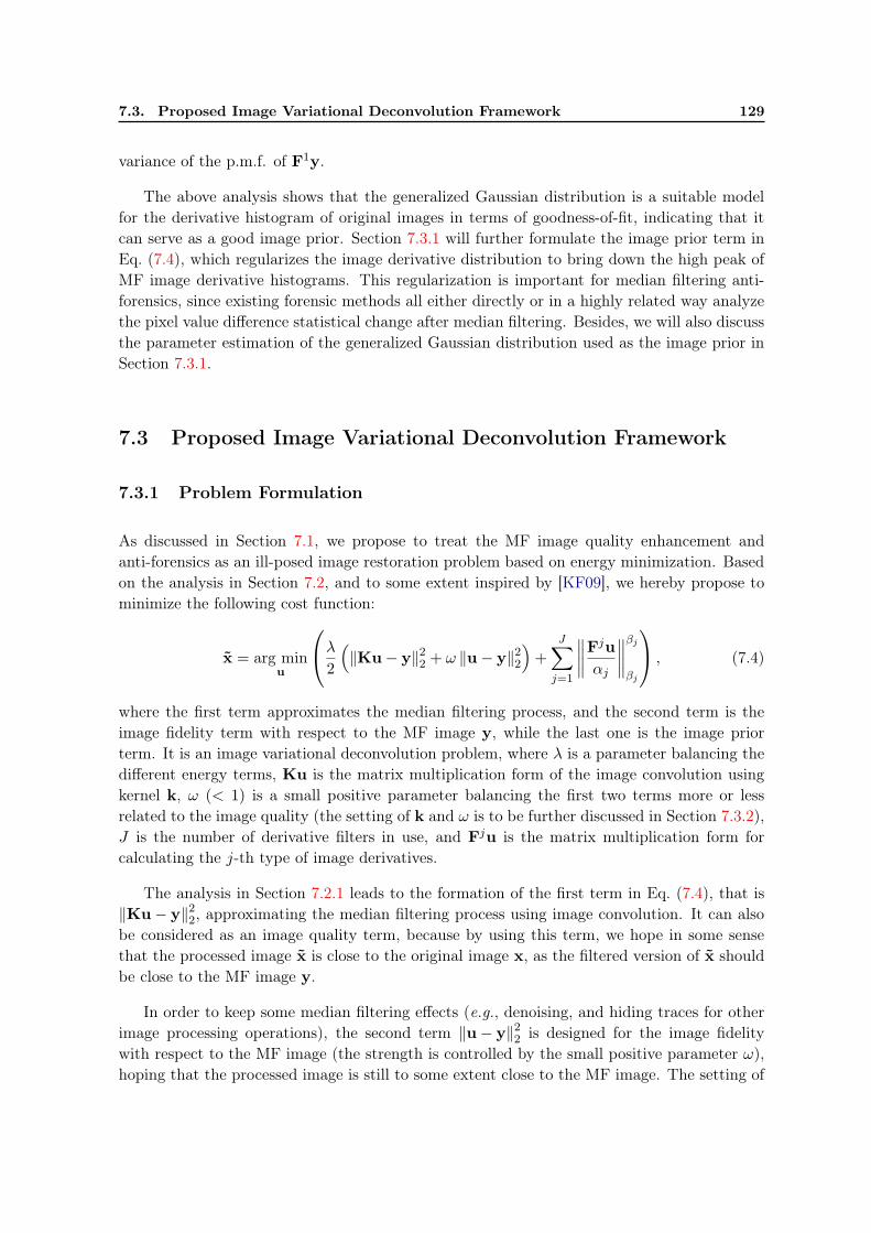
7.3. Proposed Image Variational Deconvolution Framework 129
variance of the p.m.f. of F1y.
The above analysis shows that the generalized Gaussian distribution is a suitable modelfor the derivative histogram of original images in terms of goodness-of-fit, indicating that itcan serve as a good image prior. Section 7.3.1 will further formulate the image prior term inEq. (7.4), which regularizes the image derivative distribution to bring down the high peak ofMF image derivative histograms. This regularization is important for median filtering anti-forensics, since existing forensic methods all either directly or in a highly related way analyzethe pixel value difference statistical change after median filtering. Besides, we will also discussthe parameter estimation of the generalized Gaussian distribution used as the image prior inSection 7.3.1.
7.3 Proposed Image Variational Deconvolution Framework
7.3.1 Problem Formulation
As discussed in Section 7.1, we propose to treat the MF image quality enhancement andanti-forensics as an ill-posed image restoration problem based on energy minimization. Basedon the analysis in Section 7.2, and to some extent inspired by [KF09], we hereby propose tominimize the following cost function:
x = arg minu
λ
2
(
‖Ku− y‖22 + ω ‖u− y‖22)
+
J∑
j=1
∥
∥
∥
∥
Fju
αj
∥
∥
∥
∥
βj
βj
, (7.4)
where the first term approximates the median filtering process, and the second term is theimage fidelity term with respect to the MF image y, while the last one is the image priorterm. It is an image variational deconvolution problem, where λ is a parameter balancing thedifferent energy terms, Ku is the matrix multiplication form of the image convolution usingkernel k, ω (< 1) is a small positive parameter balancing the first two terms more or lessrelated to the image quality (the setting of k and ω is to be further discussed in Section 7.3.2),J is the number of derivative filters in use, and Fju is the matrix multiplication form forcalculating the j-th type of image derivatives.
The analysis in Section 7.2.1 leads to the formation of the first term in Eq. (7.4), that is‖Ku− y‖22, approximating the median filtering process using image convolution. It can alsobe considered as an image quality term, because by using this term, we hope in some sensethat the processed image x is close to the original image x, as the filtered version of x shouldbe close to the MF image y.
In order to keep some median filtering effects (e.g., denoising, and hiding traces for otherimage processing operations), the second term ‖u− y‖22 is designed for the image fidelitywith respect to the MF image (the strength is controlled by the small positive parameter ω),hoping that the processed image is still to some extent close to the MF image. The setting of

130 Chapter 7. Median Filtered Image Quality Enhancement and Anti-Forensics
the parameter ω will be further discussed in Section 7.3.2, according to different processingpurposes of MF images.
The last term in Eq. (7.4) is the image prior term, modeling the image derivative usingthe 0-mean two-parameter generalized Gaussian distribution, based on the analysis in Sec-tion 7.2.2. It is derived by maximizing the log-likelihood of Eq. (7.2), replacing d by Fju, αby αj , and β by βj , respectively. The effect of this image prior is to regularize the distributionof the derivatives of the obtained image, so that it resembles that of the original image. In thisthesis, in total we consider J = 4 derivative filters. Besides the filter F1 defined earlier, hereF2, F3, and F4 respectively correspond to the derivative filters f2 = [1,−1]T , f3 = [1, 0,−1],and f4 = [1, 0,−1]T . Theoretically, additional image derivative filters can be added into thisframework, however leading to a high computation cost but minor impact on the final results.Moreover, it is of more importance to recover these four image derivative histograms thanothers constructed by filters where pixels in subtraction are more widely apart.
A key issue of the image prior concerns the two parameters αj and βj of the derivativedistribution of the original image. However, we cannot get access to the original image in ourtask. As shown in Section 7.2.2, the two parameters are directly related to the variance andkurtosis of the observed data. We therefore propose to use the linear regression for estimatingthe original derivative variance and kurtosis by:
σ2(Fjx) = cσ2
1 +∑M
m=1 cσ2
m+1 × σ2(
FjMF (m)(x))
,
κ(Fjx) = cκ1 +∑M
m=1 cκm+1 × κ
(
FjMF (m)(x))
,(7.5)
where σ2(·) and κ(·) respectively return the sample variance and kurtosis of the input, andcσ
2
m and cκm (m = 1, 2, · · · ,M + 1) are the linear regression coefficients. With cσ2
and cκ,the derivative variance and kurtosis of the original image can be estimated from the MFimage and its median filtered versions. In practice, the estimation accuracy improves whenM increases. In this thesis, we set M = 5, which gives us satisfying results. From the 107
images of MFPE dataset, cσ2
and cκ are obtained. The accuracy of the proposed linearprediction based estimation is quite satisfactory, for example, the mean absolute percentageerror is around 10% for the variance estimated on the MFTE dataset.
Indeed, our image variational deconvolution based problem formulation (i.e., Eq. (7.4))shares some similarities with Krishnan and Fergus’ [KF09] non-blind image deconvolutionproblem, or other image deconvolution problems in the image restoration literature. However,the two have some important differences. Firstly, the proposed problem is not a strict MAPestimate as Krishnan and Fergus’ [KF09] which is composed of a prior term and a likelihoodterm. Our cost function in Eq. (7.4) is more complex, in particular having an additionalfidelity term with respect to the MF image. Secondly, a more sophisticated image prior isemployed in our problem other than the hyper-Laplacian model for the two first-order imagederivatives used in [KF09]. The 0-mean two-parameter generalized Gaussian model has thecapability to better describe the image derivative distribution than the one-parameter hyper-Laplacian model [KF09]. Thirdly, the two generalized Gaussian parameters are adaptivelyadjusted (estimated) according to each given image, which is also different from the one fixed
7.3. Proposed Image Variational Deconvolution Framework 131
hyper-Laplacian parameter used in [KF09]. Finally, an in-depth motivation behind our imageprior modeling image derivatives is based on the specific median filtering inverse problem,where the neighboring pixel relation is prominently different before and after median filtering.Accordingly, two additional filters are adopted in the proposed image variational deconvolutionframework.
The optimization of the cost function in Eq. (7.4) is not trivial. Practically, it can be solvedby using the widely used “Half Quadratic Splitting” (see Section 2.4.3 for more descriptions)[KF09, ZW11] and the split Bregman method (see Section 2.4.4 for more descriptions) [GO09,Cha09, KTF11]. After introducing a set of auxiliary variables {wj}Jj=1 and using the “HalfQuadratic Splitting”, the optimization problem in Eq. (7.4) can be re-written as:
minu,{wj}
λ
2
(
‖Ku− y‖22 + ω ‖u− y‖22)
+J∑
j=1
(γ
2
∥
∥Fju− αjwj∥
∥
2
2+∥
∥wj∥
∥
βj
βj
)
. (7.6)
where γ is a regularization parameter.
We apply the Bregman iteration to Eq. (7.6). Thereafter, the split Bregman method solvesthe problem at the (k + 1)-th (k = 0, 1, 2, · · · ) iteration by the following formulas:
(
u(k+1), {(
wj)(k+1)}
)
= arg minu,{wj}
(
λ
2
(
‖Ku− y‖22 + ω ‖u− y‖22)
+J∑
j=1
(
γ
2
∥
∥
∥Fju+
(
bj)(k) − αjw
j∥
∥
∥
2
2+∥
∥wj∥
∥
βj
βj
)
)
,
(bj)(k+1) = (bj)(k) +(
Fju(k+1) − αj(wj)(k+1)
)
.
(7.7)where {bj}Jj=1 are the Bregman variables, and (bj)(0) = 0.
The minimization problem in Eq. (7.7) can be solved by alternating between the followingtwo sub-problems:
• w sub-problem, solving w given u. This is solved using a numerical method for differentvalues of Fju+
(
bj)(k)
, in a similar way as [KF09].
• u sub-problem, solving u given w. This quadratic problem has a closed-form solution,which can be obtained by taking the derivative of the problem with respect to u andthen setting it to 0.
In practice, we run 20 Bregman iterations, during each of which, w sub-problem and u
sub-problem are respectively solved once. For a 512× 512 MFTE image median filtered withwindow size 3 × 3, it requires around 5 seconds to process the image, using Matlab R2012bon a PC with 16G RAM and 2.80GHz CPU.
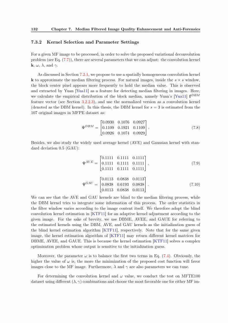
132 Chapter 7. Median Filtered Image Quality Enhancement and Anti-Forensics
7.3.2 Kernel Selection and Parameter Settings
For a given MF image to be processed, in order to solve the proposed variational deconvolutionproblem (see Eq. (7.7)), there are several parameters that we can adjust: the convolution kernelk, ω, λ, and γ.
As discussed in Section 7.2.1, we propose to use a spatially homogeneous convolution kernelk to approximate the median filtering process. For natural images, inside the s × s window,the block center pixel appears more frequently to hold the median value. This is observedand extracted by Yuan [Yua11] as a feature for detecting median filtering in images. Here,we calculate the empirical distribution of the block median, namely Yuan’s [Yua11] fDBM
feature vector (see Section 3.2.2.3), and use the normalized version as a convolution kernel(denoted as the DBM kernel). In this thesis, the DBM kernel for s = 3 is estimated from the107 original images in MFPE dataset as:
ΨDBM =
0.0930 0.1076 0.0927
0.1109 0.1921 0.1109
0.0926 0.1074 0.0929
. (7.8)
Besides, we also study the widely used average kernel (AVE) and Gaussian kernel with stan-dard deviation 0.5 (GAU):
ΨAV E =
0.1111 0.1111 0.1111
0.1111 0.1111 0.1111
0.1111 0.1111 0.1111
, (7.9)
ΨGAU =
0.0113 0.0838 0.0113
0.0838 0.6193 0.0838
0.0113 0.0838 0.0113
. (7.10)
We can see that the AVE and GAU kernels are blind to the median filtering process, whilethe DBM kernel tries to integrate some information of this process. The order statistics inthe filter window varies according to the image content itself. We therefore adopt the blindconvolution kernel estimation in [KTF11] for an adaptive kernel adjustment according to thegiven image. For the sake of brevity, we use DBME, AVEE, and GAUE for referring tothe estimated kernels using the DBM, AVE, and GAU kernels as the initialization guess ofthe blind kernel estimation algorithm [KTF11], respectively. Note that for the same givenimage, the kernel estimation algorithm of [KTF11] may return different kernel matrices forDBME, AVEE, and GAUE. This is because the kernel estimation [KTF11] solves a complexoptimization problem whose output is sensitive to the initialization guess.
Moreover, the parameter ω is to balance the first two terms in Eq. (7.4). Obviously, thehigher the value of ω is, the more the minimization of the proposed cost function will favorimages close to the MF image. Furthermore, λ and γ are also parameters we can tune.
For determining the convolution kernel and ω value, we conduct the test on MFTE100dataset using different (λ, γ) combinations and choose the most favorable one for either MF im-

7.3. Proposed Image Variational Deconvolution Framework 133
age quality enhancement or anti-forensic purposes. Here, we consider λ ∈ {1000, 2000, 3000},and γ = {300, 900, 1500}. A more fine-grained parameter grid search of (λ, γ) will be carriedout in Sections 7.3.3 and 7.3.4, after finding a proper setting for the convolution kernel andthe ω value.
In order to facilitate the parameter choosing for MF image quality enhancement, Figure 7.2shows the highest average oPSNR20 value achieved when fixing the type of kernel and the valueof ω, and varying the (λ, γ) setting. When ω = 0, the DBM kernel is able to achieve the highestoPSNR value, indicating it is the best one for median filtering process approximation amongall the 6 types of convolution kernels in consideration. This result is expected because eachelement in the DBM kernel is proportional to the probability of a pixel at a given position tobe the block median, while the AVE and GAU kernels are blind to the median filtering process.Yet, as discussed in Section 7.2.1, it is indeed oversimplified using a single convolution filterto approximate the spatially heterogeneous median filtering process. We find it is very usefulto introduce the ‖u− y‖22 term (with ω > 0) into the proposed framework of Eq. (7.4), soas to reduce the median filtering process approximation errors. From Figure 7.2, we can seethat for the three best performing kernels DBM, AVE, and AVEE, an ω value in the intervalof [0.3, 0.5] can effectively improve the oPSNR value of the processed MF image on MFTEdataset. Considering ω ∈ {0, 0.05, 0.1, 0.2, · · · , 1} and different kernels, the highest averageoPSNR value is achieved with ω = 0.4 and the AVE kernel. This setting will be adopted forMF image quality enhancement.
As to median filtering anti-forensics, the value of ω needs to be small, so that the processedimage is not too close to the MF image retaining too many median filtering artifacts. We studyseveral different values around 0.1, and observe that different ω settings have minor impact onthe final results. When ω = 0.1, the AVE and AVEE kernels outperform the other 4 kernels interms of anti-forensic performance. Take into account the image quality, the AVEE kernel isable to achieve slightly higher oPSNR, oSSIM, and mSSIM values, and 0.4585 dB of mPSNRgain on average, compared with the AVE kernel. For a better tradeoff between the forensicundetectability and image quality of the anti-forensic MF images, we choose the AVEE kernelwith ω = 0.1 as the final setting.
7.3.3 Median Filtered Image Quality Enhancement
As suggested in Section 7.3.2, we use the AVE kernel and ω = 0.4 for MF image qualityenhancement. The average oPSNR and oSSIM values can be seen in Figure 7.3, for different(λ, γ) combinations, where λ ∈ {1000, 1500, · · · , 3000} and γ ∈ {200, 300, · · · , 1000}. Com-pared with the average oPSNR value 36.8114 dB and the average oSSIM value 0.9823 for
20For evaluating the image quality, the well-known PSNR and structural similarity (SSIM) [Wan+04] metricsare used. In this thesis, we calculate the image quality metric values of the given image, using both the originalimage and the MF image as the references, under different circumstances. For the sake of clarity and to avoidconfusion, we hereafter use “oPSNR” and “oSSIM” to specifically refer to the two mentioned image metricsusing the original image as the reference, whereas “mPSNR” and “mSSIM” are for those when the MF imageserves as the reference. Note that, these notations only apply in this chapter. Besides, “PSNR” and “SSIM”still generically mean the two image quality metrics.
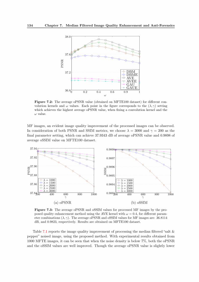
134 Chapter 7. Median Filtered Image Quality Enhancement and Anti-Forensics
ω
PSNR
0 0.2 0.4 0.6 0.9 136.8
37.2
37.6
38.0
DBMDBMEAVEAVEEGAUGAUE
Figure 7.2: The average oPSNR value (obtained on MFTE100 dataset) for different con-volution kernels and ω values. Each point in the figure corresponds to the (λ, γ) settingwhich achieves the highest average oPSNR value, when fixing a convolution kernel and theω value.
MF images, an evident image quality improvement of the processed images can be observed.In consideration of both PSNR and SSIM metrics, we choose λ = 3000 and γ = 200 as thefinal parameter setting, which can achieve 37.9343 dB of average oPSNR value and 0.9898 ofaverage oSSIM value on MFTE100 dataset.
γ
PSNR
200 400 600 800 100037.84
37.86
37.88
37.90
37.92
37.94
λ = 1000λ = 1500λ = 2000λ = 2500λ = 3000
(a) oPSNR
γ
SSIM
200 400 600 800 10000.9893
0.9894
0.9895
0.9896
0.9897
0.9898
λ = 1000λ = 1500λ = 2000λ = 2500λ = 3000
(b) oSSIM
Figure 7.3: The average oPSNR and oSSIM values for processed MF images by the pro-posed quality enhancement method using the AVE kernel with ω = 0.4, for different param-eter combinations (λ, γ). The average oPSNR and oSSIM values for MF images are: 36.8114dB, and 0.9823, respectively. Results are obtained on MFTE100 dataset.
Table 7.1 reports the image quality improvement of processing the median filtered “salt &pepper” noised image, using the proposed method. With experimental results obtained from1000 MFTE images, it can be seen that when the noise density is below 7%, both the oPSNRand the oSSIM values are well improved. Though the average oPSNR value is slightly lower

7.3. Proposed Image Variational Deconvolution Framework 135
than that of the MF image when the noise density is 7%, we can still see some oSSIM valueincrease. In Figure 7.4, example results from an MFTE image are compared, for the originalimage, the “salt & pepper” noised image, the median filtered noised image, and the processedquality enhanced image using the proposed method. It can be seen that the median filter isindeed powerful for noise removal. Yet, image blurring is also introduced, especially in theimage textured regions. The proposed method can help recover part of the information lostduring the median filtering process, with a higher image quality achieved than the MF image.
Table 7.1: The average oPSNR and oSSIM values for “salt & pepper” noised, medianfiltered, and quality enhanced images, respectively. The noise density varies from 1% to 7%.Results are obtained on MFTE dataset.
Noised Median filtered Quality enhanced
1%oPSNR 25.1365 37.1336 38.0723
oSSIM 0.8308 0.9827 0.9892
2%oPSNR 22.1257 36.9719 37.8236
oSSIM 0.7185 0.9822 0.9885
3%oPSNR 20.3642 36.7957 37.5155
oSSIM 0.6388 0.9818 0.9876
4%oPSNR 19.1161 36.6114 37.2058
oSSIM 0.5793 0.9813 0.9867
5%oPSNR 18.1466 36.4031 36.7914
oSSIM 0.5327 0.9807 0.9850
6%oPSNR 17.3540 36.1758 36.2933
oSSIM 0.4948 0.9801 0.9828
7%oPSNR 16.6851 35.8924 35.7542
oSSIM 0.4632 0.9793 0.9803
7.3.4 Anti-Forensics against Median Filtering Detection
For each forensic testing scenario, the same number of positive samples ((anti-forensic) MFimages) and negative samples (original images) are mixed for classification. Then, we can drawthe ROC curve, each point of which corresponds to a classification strategy by the detector.Thereafter, an AUC value can be calculated to quantitatively evaluate the detector’s forensicperformance (or the forensic undetectability performance of the anti-forensic image).
We consider the median filtering forensic detectors listed in Table 3.3, and use the state-of-the-art anti-forensic MF images listed in Table 3.4 for comparison. For the sake of conciseness,we also use notations for referring to the processed MF images using the methods proposedin this chapter. With the application of median filtering with s = 3 to the original image I,the MF imageM is generated, from which the following images are created:

136 Chapter 7. Median Filtered Image Quality Enhancement and Anti-Forensics
(a) Original (b) Noised
(c) Median filtered (d) Quality enhanced
Figure 7.4: Example results (close-up images) of an MFTE image. The original image (a)is contaminated by some “salt & pepper” noise of density 3% to generate (b), which is thenmedian filtered to obtain (c), which is afterwards processed for quality enhancement usingthe proposed method to create (d). Their oPSNR and oSSIM values are: (b) 20.8403 dB,0.9009; (c) 25.1402 dB, 0.9343; (d) 26.5970 dB, 0.9636, respectively.
• Mp, with the application of the MF image quality enhancement method proposed inSection 7.3.3 to the MF imageM;
• M, with the application of the proposed pixel value perturbation (to be described inSection 7.3.4.1) to the MF imageM;
• F ′M , with the application of the proposed anti-forensic method in Section 7.3.1 (withparameters properly tuned) to the MF image M;
• FM , with the application of the proposed anti-forensic method in Section 7.3.1 (withparameters properly tuned) to the perturbed MF image M.

7.3. Proposed Image Variational Deconvolution Framework 137
7.3.4.1 Pixel Value Perturbation
From Table 7.2, it can be seen that the anti-forensic performance of the processed MF imageMp using the proposed quality enhancement method in Section 7.3.3 has been improved,compared to that ofM. It implies the possibility of using the proposed framework describedin Section 7.3.1 for anti-forensic MF image creation. However, in practice, it needs more imagequality sacrifice for a further forensic undetectability improvement by pure image variationaldeconvolution. This motivates us to firstly perform some pixel value perturbation on the MFimage before further processing.
Table 7.2: From the 2nd to the 5th rows, the average PSNR and SSIM values are reported.The following 4 rows show the AUC values of different kinds of images against the 4 scalar-based detectors [KF10, Cao+10, Yua11]. The average KL divergence values of the pixel valuedifference histograms between the original images and the (quality enhanced) (anti-forensic)MF images are listed in the last 4 rows. Results are obtained on MFTE dataset.
M Mp FMW FM
D F ′M FM
Image quality
oPSNR 37.2847 38.2953 33.6033 33.4272 37.5526 37.5184
oSSIM 0.9831 0.9896 0.9552 0.9714 0.9902 0.9901
mPSNR − 43.2040 37.5618 36.4076 38.9635 38.8653
mSSIM − 0.9956 0.9713 0.9871 0.9899 0.9898
Anti-forensicperformance
KK 0.9722 0.7839 0.4592 0.5347 0.6633 0.5595
KK 0.9824 0.8375 0.6586 0.4635 0.6762 0.5061
KC 0.9938 0.8213 0.6668 0.7479 0.6690 0.6490
KY 0.9984 0.7922 0.3336 0.6518 0.6216 0.5886
KL divergence
f1 0.1632 0.0990 0.1148 0.0547 0.0571 0.0484
f2 0.1611 0.0949 0.1338 0.0563 0.0534 0.0449
f3 0.0775 0.0525 0.0619 0.0383 0.0314 0.0272
f4 0.0753 0.0495 0.0689 0.0389 0.0278 0.0238
The median filter is known to smooth the image, in a way creating (nearly) constant pixelvalues in a certain neighborhood. This can be easily detected, by analyzing the first-orderpixel value difference, e.g., by detectors KK [KF10], KK [KF10], and KC [Cao+10]. Througha careful analysis of the above mentioned detectors, we can see that their outputs are highlyrelated to the 0-valued first-order pixel value difference, especially in textured regions of theimage. Based on the above analysis and consideration, we propose to firstly perform someminor pixel value perturbation to the MF image as the following.
In the horizontal direction, let us consider three adjacent pixels denoted as a triple(yi+1,yi+2,yi+3). If yi+1 = yi+2 = yi+3, there will be two horizontal first-order pixel valuedifferences being 0, that are yi+2 − yi+1 and yi+3 − yi+2. This will directly contribute to theh0 in Eq. (3.12), leading to a high detector output of KK which may classify the given imageas median filtered. A simple but efficient adjustment is to modify the central pixel yi+2 toyi+2 ± 1. This effectively modifies the first-order statistics with a minor impact on the image

138 Chapter 7. Median Filtered Image Quality Enhancement and Anti-Forensics
quality. Similarly, we can also apply some modifications to adjacent pixel pair (yi+1,yi+2)
when yi+1 = yi+2. Based on the above analysis, we propose the following MF image pixelvalue perturbation before it is further processed for anti-forensic purposes, in the horizontaldirection followed by that in the vertical direction:
1. In the currently achieved image, find all the adjacent pixel triples (yi+1,yi+2,yi+3),where yi+1 = yi+2 = yi+3. Substitute yi+2 randomly with yi+2 + 1 or yi+2 − 1,meanwhile make sure yi+1 and yi+3 will not be touched in the subsequent modification.
2. From the updated image, find all the adjacent pixel pairs (yi+1,yi+2), where yi+1 =
yi+2. Choose between yi+1 and yi+2 with a higher local variance, update the value ofthe selected pixel by randomly incrementing or decrementing it by 1, meanwhile makesure the other pixel is not altered. In order to avoid excessive modification to the first-order pixel value difference histogram, only 30% of the equal-valued pixel pairs, withthe highest local variances, are processed.
7.3.4.2 Parameter Settings
The proposed median filtering anti-forensic method is to process the MF image obtained afterthe pixel value perturbation M, via solving the image variational deconvolution problem inEq. (7.4). According to Section 7.3.2, we set ω = 0.1 and use the AVEE kernel for medianfiltering anti-forensics. A parameter grid search is conducted to find a proper (λ, γ) combina-tion, where λ ∈ {1000, 1500, · · · , 3000} and γ ∈ {300, 400, · · · , 800}. The goal is to look for asetting which leads to a good tradeoff between forensic undetectability and image quality forthe created anti-forensic MF images.
With experiments carried out on MFTE100 dataset, Figures 7.5 and 7.6 report the varia-tion trend of the forensic undetectability and the image quality, for different settings of (λ, γ).In the existing median filtering anti-forensic work [FB12, WSL13, DN+13], the image qualitymetrics are all calculated using the MF image as the reference. However, in various appli-cations, such as denoising, hiding traces of JPEG blocking artifacts, the goal is to bring theprocessed image as close as possible to the original image. In this thesis, we therefore considerboth the original image and the MF image as the references for image quality evaluation. Notethat, in order to get a quick overview of the anti-forensic performance of the anti-forensic MFimage, for now only the scalar-based detectors (KK [KF10], KK [KF10], KC [Cao+10], andKY [Yua11]) are considered. As to the SVM-based detectors, the forensic undetectability ofthe proposed method will be reported later.
From Figure 7.5, it can be seen that the image quality improves when λ decreases or γincreases. Yet, when the value of γ is too big, the oSSIM metric suffers from some declines, andthis decrease goes faster for smaller λ values. Concerning the AUC metric, it is contradictorywith the image quality for detectorsKC andKY as shown in Figure 7.6. The AUC for Kirchnerand Fridrich’s detectors KK and KK does have a low value when the image quality is high.However, note that the closer to 0.5 the AUC value is, the better forensic undetectability the
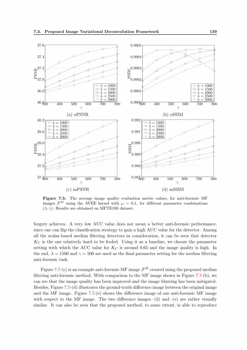
7.3. Proposed Image Variational Deconvolution Framework 139
γ
PSNR
300 400 500 600 700 80036.6
36.8
37.0
37.2
37.4
37.6
λ = 1000λ = 1500λ = 2000λ = 2500λ = 3000
(a) oPSNR
γ
SSIM
300 400 500 600 700 8000.9900
0.9901
0.9902
0.9903
0.9904
0.9905
λ = 1000λ = 1500λ = 2000λ = 2500λ = 3000
(b) oSSIM
γ
PSNR
300 400 500 600 700 80037.2
37.8
38.4
39.0
39.6
40.2λ = 1000λ = 1500λ = 2000λ = 2500λ = 3000
(c) mPSNR
γ
SSIM
300 400 500 600 700 8000.987
0.988
0.989
0.990
0.991
0.992λ = 1000λ = 1500λ = 2000λ = 2500λ = 3000
(d) mSSIM
Figure 7.5: The average image quality evaluation metric values, for anti-forensic MFimages FM using the AVEE kernel with ω = 0.1, for different parameter combinations(λ, γ). Results are obtained on MFTE100 dataset.
forgery achieves. A very low AUC value does not mean a better anti-forensic performance,since one can flip the classification strategy to gain a high AUC value for the detector. Amongall the scalar-based median filtering detectors in consideration, it can be seen that detectorKC is the one relatively hard to be fooled. Using it as a baseline, we choose the parametersetting with which the AUC value for KC is around 0.65 and the image quality is high. Inthe end, λ = 1500 and γ = 500 are used as the final parameter setting for the median filteringanti-forensic task.
Figure 7.7-(c) is an example anti-forensic MF image FM created using the proposed medianfiltering anti-forensic method. With comparison to the MF image shown in Figure 7.7-(b), wecan see that the image quality has been improved and the image blurring has been mitigated.Besides, Figure 7.7-(d) illustrates the ground-truth difference image between the original imageand the MF image. Figure 7.7-(e) shows the difference image of our anti-forensic MF imagewith respect to the MF image. The two difference images -(d) and -(e) are rather visuallysimilar. It can also be seen that the proposed method, to some extent, is able to reproduce

140 Chapter 7. Median Filtered Image Quality Enhancement and Anti-Forensics
γ
AUC
300 400 500 600 700 8000.24
0.32
0.40
0.48
0.56
0.64
λ = 1000λ = 1500λ = 2000λ = 2500λ = 3000
(a) KK [KF10]
γ
AUC
300 400 500 600 700 8000.18
0.27
0.36
0.45
0.54
0.63
λ = 1000λ = 1500λ = 2000λ = 2500λ = 3000
(b) KK [KF10]
γ
AUC
300 400 500 600 700 8000.56
0.60
0.64
0.68
0.72
0.76λ = 1000λ = 1500λ = 2000λ = 2500λ = 3000
(c) KC [Cao+10]
γ
AUC
300 400 500 600 700 8000.52
0.56
0.60
0.64
0.68λ = 1000λ = 1500λ = 2000λ = 2500λ = 3000
(d) KY [Yua11]
Figure 7.6: The anti-forensic performance against scalar-based detectors KK [KF10], KK
[KF10], KC [Cao+10], and KY [Yua11], for anti-forensic MF images FM using the AVEEkernel with ω = 0.1, for different parameter combinations (λ, γ). Results are obtained onMFTE100 dataset.
the noise-like pattern of the median filtering difference, especially in the textured areas.
Even without the pixel value perturbation, another version of our anti-forensic MF imageF ′M is also capable of creating similar noise-like pattern in the difference image with respectto the MF image shown in Figure 7.7-(e). We refrain from showing the corresponding resultdue to the fact that it is hard to check the difference between |F ′M −M| and |FM −M| byhuman naked eyes. This can also be inferred from the very small image quality metric valuedifferences between F ′M and FM (see Table 7.2). However, the median filtering anti-forensicperformance of FM is visibly improved compared with that of F ′M . We are aware that theproposed pixel value perturbation strategy for generating M is well designed for regularizingthe first-order pixel value differences 0 and ±1. Nevertheless, it can be seen that the pixelvalue perturbation has very minor impact on the image quality, but is able to achieve betterforensic undetectability, especially for the specifically targeted detectors KK and KK [KF10].Besides, the proposed pixel value perturbation is also capable of dragging the processed image

7.3. Proposed Image Variational Deconvolution Framework 141
(a) I (b)M (c) FM
(d) |I −M| (e) |FM −M|Figure 7.7: Example results (close-up images) of an MFTE image. For a better visibilityof the difference images shown in (d) and (e), we have taken logarithm of the pixel valuedifferences and afterwards carried out a normalization.
out from the detection regions of other detectors to some extent (see results for KC [Cao+10]and KY [Yua11] in Table 7.2). Moreover, the merit of the proposed pixel value perturbationcan be found in the further pixel value difference histogram restoration capability (see the KLdivergence results in Table 7.2).
Dang-Nguyen et al. [DN+13] have shown the superiority of their anti-forensic methodover Fontani and Barni’s [FB12]. We therefore refrain from the comparison with Fontani andBarni’s pioneer method [FB12]. For a fairer comparison with the other two state-of-the-artmedian filtering anti-forensic methods [WSL13, DN+13], we tune certain parameter(s) of theiralgorithms on the new forensic dataset MFTE, and choose the setting having a good tradeoffbetween forensic undetectability and image quality. Figure 7.8 shows the image quality andanti-forensic performance variations with respect to a threshold parameter T (see [DN+13]for details) of Dang-Nguyen et al.’s [DN+13] method. We choose T = 2 as the final setting,which is in accord with Dang-Nguyen et al.’s choice, though a different image dataset is inuse. A similar strategy is applied for the parameter setting of Wu et al.’s method. For thesake of brevity, the results are not shown here. Specifically, the threshold for the noise is 3,the correction factor is 0.1, and the block size is 7× 7 (see [WSL13] for details).

142 Chapter 7. Median Filtered Image Quality Enhancement and Anti-Forensics
T
AUC
1 2 3 4 5 60.3
0.4
0.5
0.6
0.7
0.8
0.9
1.0
KK
KK
KC
KY
(a) AUC
T
PSNR
1 2 3 4 5 630
32
34
36
38
40
oPSNRmPSNR
(b) PSNR
T
SSIM
1 2 3 4 5 60.96
0.97
0.98
0.99
1
oSSIMmSSIM
(c) SSIM
Figure 7.8: Anti-forensic performance against the scalar-based detectors [KF10, Cao+10,Yua11] and image quality of FM
D [DN+13], with respect to different settings of the parameterT . Results are obtained on MFTE100 dataset.
7.3.4.3 Performance Evaluation and Comparison
Table 7.2 reports the performance comparison of different kinds of (quality enhanced) (anti-forensic) MF images. ROC curves of anti-forensic MF images against the four scalar-baseddetectors [KF10, Cao+10, Yua11] are shown in Figure 7.9: among all the existing medianfiltering anti-forensic methods, ours is able to bring the ROC curves the closest to the randomguess. Besides a better overall anti-forensic performance against existing scalar-based medianfiltering detectors, our anti-forensic MF image FM also outperforms Wu et al.’s FM
W [WSL13]and Dang-Nguyen et al.’s FM
D [DN+13] in terms of image quality. Moreover, it is worthnoticing that our anti-forensic MF image FM also achieves even higher average oPSNR andoSSIM values than the MF image M on MFTE dataset. It means that the proposed medianfiltering anti-forensic method is not only able to disguise the median filtering traces, but isalso capable of improving the visual quality of the MF image at the same time.

7.3. Proposed Image Variational Deconvolution Framework 143
False positive rate
Truepositiverate
0 0.2 0.4 0.6 0.8 10
0.2
0.4
0.6
0.8
1
KK
KK
KC
KY
Random guess
(a)MFalse positive rate
Truepositiverate
0 0.2 0.4 0.6 0.8 10
0.2
0.4
0.6
0.8
1
KK
KK
KC
KY
Random guess
(b) FMW
False positive rate
Truepositiverate
0 0.2 0.4 0.6 0.8 10
0.2
0.4
0.6
0.8
1
KK
KK
KC
KY
Random guess
(c) FMD
False positive rate
Truepositiverate
0 0.2 0.4 0.6 0.8 10
0.2
0.4
0.6
0.8
1
KK
KK
KC
KY
Random guess
(d) FM
Figure 7.9: ROC curves of the MF image M, Wu et al.’s anti-forensic MF image FMW
[WSL13], Dang-Nguyen et al.’s anti-forensic MF image FMD [DN+13], and our anti-forensic
MF image FM , against the four scalar-based median filtering detectors KK [KF10], KK
[KF10], KC [Cao+10], and KY [Yua11]. Results are obtained on MFTE dataset.
Existing median filtering forensic work either explicitly or implicitly analyzes the pixelvalue difference. Therefore, besides the forensic undetectability and image quality, it is alsoimportant to recover the pixel value difference statistics for median filtering anti-forensics.This can be quantitatively evaluated, via the KL divergence (see Section 2.2.3 for more de-scriptions) between the derivative histogram of the original image and that of the image underexamination. A smaller value of KL divergence means a better resemblance between the twocompared histograms. We consider four derivative filters f1, f2, f3, and f4. For each imageunder investigation, each type of derivative histogram is constructed and compared with thatof the original image using the KL divergence. The average KL divergence values between

144 Chapter 7. Median Filtered Image Quality Enhancement and Anti-Forensics
the original image and different kinds of images for different kinds of derivative histogramsare reported in the last four rows of Table 7.2. It can be seen that the proposed method hasthe ability to bring the pixel value difference histogram closer to that of the original imagethan the two state-of-the-art methods [WSL13, DN+13]. This proves the pixel value differ-ence statistics restoration capability of the image prior we use in the proposed optimizationproblem. It is also an interesting point that the proposed pixel value perturbation strategy iscapable of bringing the derivative histogram of the anti-forensic MF image FM even closer tothat of the original image than the other version of our anti-forensic MF image F ′M .
Concerning the SVM-based detectors, we follow the testing strategy described in Sec-tion 2.2.1.2. For a given original image, a square central part of the image is re-placed by the (anti-forensic) MF image with a replacement rate around the values in{0.05, 0.1, 0.15, 0.2, 0.3, 0.4, 0.5, 0.6, 0.8, 1} to create the image forgery. The processed imagestogether with the original images are put together for forensic training/testing. The training iscarried out using LIBSVM [CL11] with a Gaussian kernel on dataset MFTR. The parametersof the SVM classifier is obtained using a five-fold cross validation with the multiplicative gridsuggested in [PBF10]. The testing is carried out on dataset MFTE. Thereafter, for each imagereplacement rate, each kind of (anti-forensic) MF image, and each kind of SVM-based medianfiltering forensic detector, a ROC curve can be plotted and an AUC value can be calculated.The AUC curve as a function of the replacement rate is plotted in Figure 7.10 by differentkinds of images and different kinds of SVM-based detectors.
The effectiveness of existing SVM-based median filtering forensic detectors [PBF10, Yua11,CNH13, Kan+13, Zha+14] in discriminating (anti-forensic) MF images from the original im-ages can be evaluated when the replacement rate is 1. From Figure 7.10, it can be seen thatthey all perform excellently, and are able to achieve AUC values around 1, namely perfectclassification. Except for detector KS10
AR [Kan+13], our anti-forensic MF image FM achievesthe best forensic undetectability against the considered SVM-based detectors among all kindsof (anti-forensic) MF images. Moreover, the performance of our forgery FM is quite stable,yielding AUC values almost at the same level for the same replacement rate for different SVM-based detectors. When the replacement rate is about 0.1, our anti-forensic MF image FM isable to achieve AUC values lower than 0.65 for all considered SVM-based detectors. In thiscase, we can safely replace a 162×162 block in a 512×512 MFTE image. We remain reservedon whether our anti-forensic MF image is able to pass off as never median filtered, since itcan be detected by machine learning based forensic methods, when the replacement rate isrelatively high. However, it can still find many applications in various anti-forensic scenarios,e.g., image splicing and tampering with relatively low replacement rate.
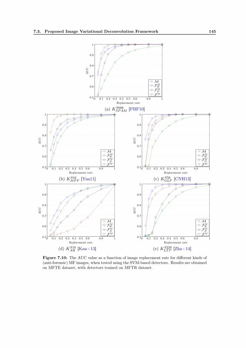
7.3. Proposed Image Variational Deconvolution Framework 145
Replacement rate
AUC
0 0.1 0.2 0.3 0.4 0.5 0.6 0.8 10.5
0.6
0.7
0.8
0.9
1
M
FM
W
FM
D
FM
(a) KS686SPAM [PBF10]
Replacement rate
AUC
0 0.1 0.2 0.3 0.4 0.5 0.6 0.8 10.5
0.6
0.7
0.8
0.9
1
M
FM
W
FM
D
FM
(b) KS44MFF [Yua11]
Replacement rate
AUC
0 0.1 0.2 0.3 0.4 0.5 0.6 0.8 10.5
0.6
0.7
0.8
0.9
1
M
FM
W
FM
D
FM
(c) KS56GLF [CNH13]
Replacement rate
AUC
0 0.1 0.2 0.3 0.4 0.5 0.6 0.8 10.5
0.6
0.7
0.8
0.9
1
M
FM
W
FM
D
FM
(d) KS10AR [Kan+13]
Replacement rate
AUC
0 0.1 0.2 0.3 0.4 0.5 0.6 0.8 10.5
0.6
0.7
0.8
0.9
1
M
FM
W
FM
D
FM
(e) KS220LTP [Zha+14]
Figure 7.10: The AUC value as a function of image replacement rate for different kinds of(anti-forensic) MF images, when tested using the SVM-based detectors. Results are obtainedon MFTE dataset, with detectors trained on MFTR dataset.
146 Chapter 7. Median Filtered Image Quality Enhancement and Anti-Forensics
7.4 Applications: Disguising Footprints of Both Median Fil-tering and Targeted Image Operation of Median FilteringProcessing
Median filtering is chosen by many forgers to disguise footprints left by certain image pro-cessing operations, e.g., image resampling [KR08], and JPEG compression [SL11]. Medianfiltering anti-forensics further tries to remove the footprints caused by the filtering itself. It isimportant that median filtering anti-forensics does not impair the trace removal effects of thefiltering initially applied, while keeping a high quality of the processed image.
7.4.1 Hiding Traces of Image Resampling
It is a very likely scenario for a forger, e.g., during a composite image forgery creation, to usethe scaling operation. Thus, image resampling is often involved in creating fake images. On theforensic investigation side, Popescu and Farid [PF05] proposed a powerful resampling forensicdetector (denoted as KP ), by examining the periodic correlations between pixel neighbors.Standing on the image resampling anti-forensic side, Kirchner and Röhme [KR08] developeda technique which was able to fool KP [PF05], via attacks based on median filtering andgeometric distortion.
As in [PF05], we use bicubic interpolation for image resampling, and the factors in use arerandomly selected from {0.7, 0.8, 0.9, 1.1, 1.2}. The 3× 3 median filtering alone (without geo-metric distortion applied) works well under these scaling factors, for resampling anti-forensicpurposes [KR08].
For the sake of conciseness, we create different anti-forensic images from the resampledimage R as follows:
• Rm, median filtered with window size s = 3;
• Rw, with the application of Wu et al.’s [WSL13] median filtering anti-forensic methodto Rm;
• Rd, with the application of Dang-Nguyen et al.’s [DN+13] median filtering anti-forensicmethod to Rm;
• Rf , with the application of the proposed median filtering anti-forensic method to Rm.
Table 7.3 reports the image quality and forensic undetectability against Popescu andFarid’s resampling forensic detector [PF05] and the scalar-based median filtering detectors[KF10, Cao+10, Yua11], for different kinds of anti-forensic MF images created from the re-sampled image R. Moreover, the 5 SVM-based median filtering detectors are also tested,following the experimental setup described in Section 2.2.1.2. Figure 7.11 plots the achieved

7.4. Applications of Median Filtering Anti-Forensics 147
AUC values by different kinds of images, against different SVM-based median filtering forensicdetectors at different replacement rates.
Table 7.3: From the 2nd to the 5th rows, the average PSNR and SSIM values are reportedfor different kinds of images in the resampling traces hiding application. The last 5 rowsshow the AUC values of different kinds of images against the resampling detector [PF05] andthe 4 scalar-based median filtering detectors [KF10, Cao+10, Yua11]. Results are obtainedon MFTE dataset.
R Rm Rw Rd Rf
Image quality
rPSNR − 37.9091 33.7600 33.3101 37.2413
rSSIM − 0.9749 0.9391 0.9711 0.9894
mrPSNR 37.9091 − 37.5393 36.3006 38.8262
mrSSIM 0.9749 − 0.9618 0.9870 0.9896
Anti-forensicperformance
KP 0.8643 0.6818 0.9834 0.5001 0.6495
KK 0.3775 0.9672 0.4289 0.5129 0.5364
KK 0.2792 0.9782 0.6113 0.4422 0.4599
KC 0.4834 0.9929 0.6511 0.7356 0.6386
KY 0.5096 0.9984 0.3212 0.6424 0.5876
Since the resampling changes the pixel locations, it is not straightforward to calculate theimage quality metric values with the original image as the reference. Hence, the resampledimage (for “rPSNR” and “rSSIM”) and the median filtered resampled image (for “mrPSNR” and“mrSSIM”) are used as the references. Table 7.3 shows the superiority of the proposed methodin keeping a good image quality. Our forgery Rf achieves 4.34 dB of rPSNR enhancement and0.0443 of rSSIM gain compared with Rw, and 4.53 dB of rPSNR improvement and 0.0219 ofrSSIM increase compared with Rd. Using the image quality evaluation metrics mrPSNR andmrSSIM, our forgery Rf also outperforms Rw [WSL13] and Rd [DN+13]. Moreover, both theaverage rPSNR and rSSIM values of Rf are even higher than the median filtered image Rm.
Concerning Popescu and Farid’s resampling detector KP [PF05], it can be seen that bothDang-Nguyen et al.’s [DN+13] and the proposed median filtering anti-forensic methods caneven reinforce the anti-forensic ability of median filtering in hiding resampling traces. Thisis reflected by the even lower AUC values of detector KP , compared with that of Rm (seeTable 7.3). However, our forgery can achieve a better overall forensic undetectability againstthe median filtering detectors than Rd [DN+13] (see results in Table 7.3 and Figure 7.11).Wu et al.’s forgery Rw can be well detected by KP . Recall that their method is based onthe noise attack to the pixel value difference. In their approach, the given image is dividedinto non-overlapping blocks, each of which has an anchor point as the reference of the noiseattack to alter the pixel value differences. This block-wise pixel modification may invokethe appearance of new periodicity of pixel neighbor correlation, which consequently can bedetected by KP . A randomized anchor point selection may be a possible improvement to thisapproach, which however is beyond the scope of this thesis.

148 Chapter 7. Median Filtered Image Quality Enhancement and Anti-Forensics
Replacement rate
AUC
0 0.1 0.2 0.3 0.4 0.5 0.6 0.8 10.5
0.6
0.7
0.8
0.9
1
Rm
Rw
Rd
Rf
(a) KS686SPAM [PBF10]
Replacement rate
AUC
0 0.1 0.2 0.3 0.4 0.5 0.6 0.8 10.5
0.6
0.7
0.8
0.9
1
Rm
Rw
Rd
Rf
(b) KS44MFF [Yua11]
Replacement rate
AUC
0 0.1 0.2 0.3 0.4 0.5 0.6 0.8 10.5
0.6
0.7
0.8
0.9
1
Rm
Rw
Rd
Rf
(c) KS56GLF [CNH13]
Replacement rate
AUC
0 0.1 0.2 0.3 0.4 0.5 0.6 0.8 10.5
0.6
0.7
0.8
0.9
1
Rm
Rw
Rd
Rf
(d) KS10AR [Kan+13]
Replacement rate
AUC
0 0.1 0.2 0.3 0.4 0.5 0.6 0.8 10.5
0.6
0.7
0.8
0.9
1
Rm
Rw
Rd
Rf
(e) KS220LTP [Zha+14]
Figure 7.11: The AUC value as a function of image replacement rate for different kindsof images, when tested using the SVM-based median filtering forensic detectors, in theresampling traces hiding application. Results are obtained on MFTE dataset, with detectorstrained on MFTR dataset.

7.4. Applications of Median Filtering Anti-Forensics 149
7.4.2 Removing JPEG Blocking Artifacts
We have studied JPEG anti-forensics in Chapters 4-6. As known, two kinds of artifacts presentin JPEG images, i.e., the DCT-domain quantization artifacts and the spatial-domain blockingartifacts, which are often utilized for JPEG forensic purposes. The consistent discontinuitiesacross 8 × 8 block borders, i.e., the JPEG blocking artifacts, can be detected by detectorsKF [FD03], K1
U and K2U (see Table 3.1). In one state-of-the-art JPEG anti-forensic method
[Sta+10a, Sta+10b, SL11], Stamm and Liu separated the task of disguising the JPEG foot-prints into two steps: adding a dithering signal to smooth the DCT histogram followed bya median filtering based JPEG blocking artifact removal procedure. During the second step,they proposed a JPEG deblocking process consisting of a median filtering and a small-energy0-mean white Gaussian noise addition (see Section 3.1.5 for more descriptions).
In order to purely study the footprint concealing capability of median filtering, here weapply the median filtering directly to JPEG images without the noise attack. The JPEGcompression quality factors in use are randomly selected from {85, 86, · · · , 95}. We find thatfor JPEG images with quality factors in this set, the median filtering alone can perform verywell in concealing JPEG blocking artifacts.
We use the following notations to refer to different anti-forensic images created from theJPEG image J :
• Jm, median filtered with s = 3;
• J w, with the application of Wu et al.’s [WSL13] median filtering anti-forensic methodto Jm;
• J d, with the application of Dang-Nguyen et al.’s [DN+13] median filtering anti-forensicmethod to Jm;
• J f , with the application of the proposed median filtering anti-forensic method to Jm.
The average image quality and anti-forensic performance against JPEG blocking detectorsand scalar-based median filtering detectors are reported in Table 7.4. At different replacementrates, the AUC values achieved by different anti-forensic images tested against 5 SVM-basedmedian filtering detectors are shown in Figure 7.12. Note that “mjPSNR” and “mjSSIM”respectively stand for the PSNR and SSIM metrics, when the median filtered JPEG imageis used as the reference. It can be seen that our forgery FM is able to achieve a betteroverall forensic undetectability against the median filtering detectors than J w [WSL13], andJ d [DN+13]. As to JPEG blocking artifacts hiding, all the three kinds of anti-forensic MFimages are able to even further decrease the AUC values of detectors KF [FD03], K1
U , and K2U
[Fan+13a]. However, the price for J w and J d is an evident image degradation: an oPSNRloss of 3.58 dB and 3.78 dB compared to Jm on average, respectively. As to our forgery J f ,not only a good overall forensic undetectability is guaranteed, but also an oPSNR gain of 0.15dB and a slight oSSIM increase are achieved, compared with Jm. Moreover, the mjPSNR and

150 Chapter 7. Median Filtered Image Quality Enhancement and Anti-Forensics
mjSSIM values achieved by our forgery J f are also both higher than those of J w [WSL13]and J d [DN+13].
Table 7.4: From the 2nd to the 5th rows, the average PSNR and SSIM values are reportedfor different kinds of images in the JPEG blocking artifacts removing application. The last7 rows show the AUC values of different kinds of images against JPEG blocking detectors[FD03] and the 4 scalar-based median filtering detectors [KF10, Cao+10, Yua11]. Resultsare obtained on MFTE dataset.
J Jm J w J d J f
Image quality
oPSNR 42.9742 37.0888 33.5111 33.3101 37.2413
oSSIM 0.9975 0.9830 0.9549 0.9711 0.9894
mjPSNR 37.6087 − 37.4983 36.3006 38.8262
mjSSIM 0.9838 − 0.9710 0.9870 0.9896
Anti-forensicperformance
KF 0.9930 0.6128 0.6321 0.4945 0.6003
K1U 0.9871 0.7151 0.5709 0.6255 0.5168
K2U 0.8937 0.5288 0.5363 0.5274 0.4754
KK 0.3895 0.9659 0.4109 0.5035 0.5137
KK 0.2699 0.9786 0.6061 0.4256 0.4489
KC 0.3990 0.9924 0.6369 0.7230 0.6244
KY 0.4985 0.9986 0.3225 0.6489 0.5976
7.5 Summary
In this chapter, we continue the research line of leveraging on image restoration to designmedian filtering anti-forensic method, similar to what we did in JPEG anti-forensics in Chap-ters 4-6. More specifically, we have proposed an image variational deconvolution framework,which can serve as an MF image quality enhancement method as well as an MF image anti-forensic approach. Indeed, a single convolution filter is used to approximate the spatiallyheterogeneous median filter. It may appear to be somewhat irrational but makes the problemsolvable, and in practice yields good results. The image prior adopts the generalized Gaussiandistribution to model image derivatives. It is a simple yet especially suitable prior for MFimage quality enhancement and anti-forensics. The median filter largely alters the statisticsin the pixel value difference domain, whereas the proposed prior is able to well regularize thepixel value difference histogram, which is proven in experiments by a low KL divergence valuewith respect to the histogram of the original image.
For anti-forensic purposes, a pixel value perturbation strategy is proposed to process theMF image in advance, with a very minor impact on the visual quality of the final forgery.Experimental results show that our anti-forensic MF image outperforms the state-of-the-artanti-forensic MF images in terms of forensic undetectability, with an even higher image qualitythan the MF image on MFTE dataset. Moreover, backed by experiments, the proposed median

7.5. Summary 151
Replacement rate
AUC
0 0.1 0.2 0.3 0.4 0.5 0.6 0.8 10.5
0.6
0.7
0.8
0.9
1
J m
J w
J d
J f
(a) KS686SPAM [PBF10]
Replacement rate
AUC
0 0.1 0.2 0.3 0.4 0.5 0.6 0.8 10.5
0.6
0.7
0.8
0.9
1
J m
J w
J d
J f
(b) KS44MFF [Yua11]
Replacement rate
AUC
0 0.1 0.2 0.3 0.4 0.5 0.6 0.8 10.5
0.6
0.7
0.8
0.9
1
J m
J w
J d
J f
(c) KS56GLF [CNH13]
Replacement rate
AUC
0 0.1 0.2 0.3 0.4 0.5 0.6 0.8 10.5
0.6
0.7
0.8
0.9
1
J m
J w
J d
J f
(d) KS10AR [Kan+13]
Replacement rate
AUC
0 0.1 0.2 0.3 0.4 0.5 0.6 0.8 10.5
0.6
0.7
0.8
0.9
1
J m
J w
J d
J f
(e) KS220LTP [Zha+14]
Figure 7.12: The AUC value as a function of image replacement rate for different kindsof images, when tested using the SVM-based median filtering forensic detectors, in theJPEG blocking artifacts removing application. Results are obtained on MFTE dataset,with detectors trained on MFTR dataset.
filtering anti-forensic method is effective in applications of disguising image resampling tracesand JPEG blocking artifacts.


Chapter 8
Conclusions
8.1 Summary of Contributions
In this thesis, we have presented our research work on image anti-forensics to JPEG com-pression and median filtering. During our study of image anti-forensics concerning imagecoding/processing, we notice that it to some extent shares some similarities with image restora-tion. Both of them aim to recover the information lost during the image degradation to theutmost. However, besides image quality, image anti-forensics has an additional indispensablegoal, i.e., good forensic undetectability of the anti-forensic image against forensic detectors.To this end, we introduce some advanced concepts/methods from image restoration to de-sign new anti-forensic methods, meanwhile integrating some anti-forensic strategies/terms.Experimental results demonstrate that the proposed anti-forensic methods outperform thestate-of-the-art methods in creating anti-forensic images with better forensic undetectabilityagainst existing forensic detectors as well as a higher visual quality of the processed image.Though image restoration itself is not our main research topic in this thesis, we also pro-pose two image quality enhancement methods for JPEG compression and median filtering,respectively. They serve as the preliminary step of the proposed anti-forensic methods, butare also proven to have good performance in terms of PSNR and SSIM gains compared withthe JPEG/MF image.
The contributions of this thesis are summarized as follows.
Proposing a new research line of designing image anti-forensics via image restora-tion: After conducting the literature review, we find that it is a common way to use simpleimage processing for hiding traces left by a targeted operation to design image anti-forensics.For example, median filtering is used for JPEG anti-forensics to remove blocking artifacts.Noise injection is used to hide traces of median filtering. These methods can be effective inattacking targeted forensic detectors, however can also be detected by more advanced detec-tors. Moreover, the resulting anti-forensic image suffers from a low visual quality, which mayspontaneously cause the doubt upon its authenticity. In this thesis, we propose a new researchline of designing image anti-forensics leveraging on advanced concepts/methods from imagerestoration. Given a degraded image processed by an irreversible image processing operation,e.g., JPEG compression and median filtering, the objective of image anti-forensics is to hidethe relevant image processing traces meanwhile maintaining a good image quality of the anti-forensic image. Based on the similarities between image anti-forensics and image restoration,the introduced optimization framework/terms from image restoration help to partly remove
153

154 Chapter 8. Conclusions
the traces, while keeping a good (sometimes even higher) image quality compared with thegiven degraded image. Good anti-forensic performance of the image is achieved by addinganti-forensic terms to the optimization framework or using additional anti-forensic strategies.We follow this research line throughout this thesis for JPEG anti-forensics as well as medianfiltering anti-forensics. Its superiority over state-of-the-art anti-forensic methods is well provenby experimental results, with a better forensic undetectability and a higher image quality ofthe processed image. To the best of our knowledge, we are the first to conduct image anti-forensics following this research direction. We also hope this new research line would be usefulin more image anti-forensic problems when image coding/processing is involved, e.g., imageresampling, contrast enhancement, etc.
JPEG anti-forensics using TV-based deblocking: We have proposed a JPEG anti-forensic method using the TV-based deblocking method. This is implemented by optimizinga constrained TV-based minimization problem with a TV term and a TV-based blockingmeasurement term. Meanwhile, the visual quality of the processed image is controlled by amodified QCS projection. Moreover, the powerful calibration based detector is defeated byminimizing a cost function close to the calibration based JPEG forensic feature. This methodhas good performance in spatial-domain JPEG blocking artifacts removal. Besides, the DCT-domain quantization artifacts are also largely mitigated, to the extent that the anti-forensicJPEG image is able to pass off as never compressed under the examination of quantizationartifacts detectors.
Improved JPEG anti-forensics with perceptual DCT histogram smoothing: Indeed,the previously proposed TV-based JPEG deblocking method is able to achieve good foren-sic undetectability against all existing JPEG forensic detectors including the ones examiningquantization artifacts. However, the DCT histogram is still not always well smoothed espe-cially in the mid-frequency subbands. This weakness is not exposed by existing JPEG forensicdetectors, yet may be detected by potential, more advanced forensic algorithms. In order totackle this problem, we have proposed a four-step improved JPEG anti-forensic method withperceptual DCT histogram smoothing. With the help of the partly recovered DCT coefficientsafter the TV-based deblocking, an adaptive local dithering method is proposed by combiningthe Laplacian distribution and the uniform distribution. DCT coefficients are modified bysolving a simplified assignment problem which minimizes the SSIM loss in the spatial do-main. A mild second-round TV-based deblocking and de-calibration are performed to furtherimprove the forensic undetectability with a very minor image quality loss.
JPEG image quality enhancement and anti-forensics using a sophisticated imageprior model: We have proposed another JPEG anti-forensic method based on a sophisticatedimage prior model, which are described by steps in the following.
• JPEG image quality enhancement with a sophisticated image prior model : The effective-ness of using TV in JPEG anti-forensics motivates us to seek more sophisticated imageprior models, with the hope to further push the performance of JPEG anti-forensics.To this end, we use the EPLL framework with the GMM as the image prior modelfor overlapping image patches. The spatial-domain compression noise is modeled using
8.1. Summary of Contributions 155
the multivariate 0-mean Gaussian model, for which 64 kinds of covariance matrices arelearned for each quality factor. Therefore, a JPEG image quality enhancement methodhas been proposed by minimizing the cost function considering the above two terms.The quality enhanced JPEG image can be obtained by solving an optimization prob-lem using one step of approximate MAP estimation. This method achieves good imagequality gain for JPEG images, especially for very low bit-rate compression.
• Calibration based non-parametric DCT histogram smoothing : Compared with our pre-viously proposed perceptual DCT histogram smoothing method, we also have proposedanother calibration based DCT histogram smoothing procedure without using any statis-tical model. Based on the translation invariance of image statistics and the effectivenessof calibration, the DCT-domain quantization noise can be estimated by slightly croppingthe quality enhanced JPEG image and recompressing the calibrated image. The DCThistogram is smoothed by adding the estimated DCT-domain quantization noise back tothe quality enhanced JPEG image. This new, non-parametric DCT histogram smooth-ing method does not achieve a better overall performance but has better performancein the low-frequency DCT subbands than the perceptual DCT histogram smoothingmethod. Moreover, the former has a much lower computation cost than the latter.
• Forensic undetectability is considered by minimizing a cost function with an image fi-delity term, an EPLL-based image prior term, and several anti-forensic terms inspiredfrom existing forensic algorithms.
To recapitulate, the proposed quality enhancement method is proven by experiments on 4classical test images and on UCIDTest dataset to improve the visual quality of the JPEGimage. Indeed, the proposed anti-forensic method needs improvement, however still outper-forms Stamm et al.’s method [Sta+10a, Sta+10b, SL11] in terms of forensic undetectabilityand visual quality of the processed image.
Median filtered image quality enhancement and anti-forensics via variational de-convolution: We have proposed an MAP-based image variational deconvolution frameworkfor both median filtered image quality enhancement and anti-forensics. The median filteringprocess is approximated using a convolution kernel. Besides, we also hope the processed MFimage is still to some extent close to the MF image, retaining some median filtering effectssuch as denoising or artifacts hiding for other image operations. As to the image prior, thegeneralized Gaussian distribution is used to model the pixel value difference whose statisticschanges largely after the image is median filtered. Based on the above consideration, theproposed minimization cost function is formed by a convolution term, a fidelity term withrespect to the MF image, and a prior term. The quality enhanced MF image can be obtainedby solving the proposed minimization problem, with good visual quality gain compared tothe MF image. With another parameter setting and an additional pixel value perturbationprocedure, the anti-forensic MF image is also generated. It is able to achieve a better forensicundetectability against existing median filtering forensic detectors and a higher image quality,compared with the state-of-the-art anti-forensic MF images.
In summary, the main characteristic/novelty of this thesis is to introduce advanced

156 Chapter 8. Conclusions
concepts/methods from image restoration to design image anti-forensics, when image cod-ing/processing is involved. More specifically, we have designed JPEG anti-forensics and me-dian filtering anti-forensics, leveraging on the following elements from image restoration: theTV, the EPLL framework with GMM as the prior model for overlapping image patches, theMAP-based image deconvolution framework. For a given specific image anti-forensic problem,some anti-forensic terms/strategies are integrated for defeating existing detectors. For JPEGcompression, a TV-based blocking measurement term is used for JPEG deblocking purposes.Moreover, two DCT histogram smoothing methods are also proposed to remove DCT-domainquantization artifacts: a perceptual DCT histogram smoothing procedure conducted by build-ing an adaptive local dithering model and solving a simplified assignment problem, and anon-parametric DCT histogram smoothing method based on calibration. Some anti-forensicterms inspired from existing forensic algorithms are also integrated into the MAP-based opti-mization framework, for fooling relevant forensic detectors. As to median filtering, the imageprior model is specifically chosen to regularize the image pixel value differences, which are ei-ther explicitly or implicitly examined in existing forensic algorithms. Moreover, a pixel valueperturbation procedure is also proposed to further improve the forensic undetectability withvery minor visual quality loss of the processed image.
8.2 Perspectives
In the short term, the perspectives of this thesis include the performance improvement ofanti-forensics, and applying the research line of leveraging on image restoration to designalgorithms to solve other suitable image anti-forensic problems. Please see the following formore detailed descriptions.
Improvement of JPEG anti-forensics to generate the anti-forensic image with aneven higher quality than the JPEG image: In Chapters 4-5, the TV is employed fromimage restoration to JPEG anti-forensics. The TV can be considered as a simple but ef-fective image prior. Chapter 6 presents the natural follow-up work on JPEG anti-forensics,where a more sophisticated image prior model than the TV is used. However, the new JPEGanti-forensic method does not outperform the ones based on the TV. Analysis and possibleunderlying reasons are provided in the end of Sections 6.3 and 6.4. However, we can stillsee the effectiveness of the proposed JPEG quality enhancement method based on the EPLLframework with the GMM as the image prior model. A challenging but very interesting JPEGanti-forensic problem is whether we are able to create anti-forensic JPEG image with an evenhigher visual quality than the JPEG image. A possible research direction could be the combi-nation of the JPEG image quality enhancement, the TV-based deblocking, and the perceptualsmoothing of DCT histogram. In fact, a similar goal has already been achieved in Chapter 7for median filtering anti-forensics: the anti-forensic MF image is created with an even highervisual quality than the MF image on MFTE dataset.
Development of other image anti-forensic methods leveraging on image restora-tion: In this thesis, we choose to work on JPEG compression and median filtering anti-

8.2. Perspectives 157
forensics. In image processing, there are various other image operations whose anti-forensicsmay also be formulated as ill-posed inverse problems. For example, image resampling anti-forensics may share some similarities with superresolution [PPK03]. Image contrast enhance-ment anti-forensics may be related to the estimation of pixel brightness transform [ZL14]. Ide-ally, a good performance of the anti-forensic method can be achieved if these concepts/methodsfrom image restoration are well combined with some anti-forensic terms/strategies.
In the long term, one of the ultimate goals of image forensics and anti-forensics is todevelop universal methods without targeting at a specific (set of) anti-forensic methods orforensic algorithms. This is to avoid the endless cat-and-mouse chasing between forensics andanti-forensics. Though the research work of image (anti-)forensics has been going on for over adecade, there are very few universal methods. Probably the only universal image anti-forensicmethod is the one proposed by Barni et al. [BFT12]. However, they also make the assumptionthat the forensic detectors examine the first-order statistics only. We are aware that theproposed anti-forensic methods all belong to the “targeted” category according to Böhme andKirchner’s [BK13] classification of image anti-forensics (see Section 2.1.5). However, we believethe proposed anti-forensic methods have the potential to be further generalized for developinguniversal image anti-forensics.
Universal image anti-forensics: In Chapters 6-7, the MAP-based optimization problemsare proposed to perform JPEG anti-forensics and median filtering anti-forensics, respectively.The universality of the variational image restoration framework can be seen through thesetwo problems. When it concerns image coding/processing, the objective of anti-forensics is tocreate anti-forensic images that are as “natural” as possible. To this end, the “natural” imagegeneration problem can be formulated as an image restoration problem and use statisticalmethods, such as MAP estimate, to obtain an image that appears never processed. Underthis framework, a good enough image prior model is indispensable. Moreover, the likelihoodterm, describing the image degradation process caused by a certain image operation, shouldvary according to different anti-forensic problems. The “universality” here is that the anti-forensic framework is generic, which can be used to hide the traces left by various imageprocessing operations.
Besides, some other open research problems closely related to this thesis are listed asfollows:
• Is it possible to design a single step attack for JPEG anti-forensics, considering multipleforensic detectors working in different domains?
• How can we estimate the spatially heterogeneous convolution kernel for median filtering?
• Is it possible to create anti-forensic image, so that it as a whole can pass off as neverprocessed by machine learning based forensic detectors trained on the original imagesand anti-forensic images?
These questions also point out a few interesting future research directions in the vast domainof image anti-forensics. Moreover, concerning the close link between digital images and digital

158 Chapter 8. Conclusions
videos, the proposed image anti-forensic methods to JPEG compression and median filteringmay also contribute to video anti-forensics.
In this thesis, we conduct the study on JPEG anti-forensics and median filtering anti-forensics following the research line of leveraging on image restoration. These two specificimage anti-forensic problems just constitute a small fraction of image anti-forensics. We arealso aware that this newly formed research line may be only applied to image anti-forensicproblems, where image coding/processing is involved. For other image anti-forensic problems,e.g., attacking physically based or geometric-based [Far09a] forensic algorithms, this researchline may be invalid. For example, in our lighting-based image anti-forensic work [Fan+12], avery different research line is followed.
In conclusion, for image anti-forensic problems involving image coding/processing, webelieve that natural image statistics is essential in creating the anti-forensic image withgood forensic undetectability as well as a high visual quality. To this end, some ad-vanced concepts/methods from image restoration are introduced to combine with anti-forensicterms/strategies in this thesis for JPEG anti-forensics and median filtering anti-forensics.From our image anti-forensic research work conducted following this research line, we cancatch a glimpse of the enormous potential of natural image statistics in image anti-forensics,image forensics and image restoration. Böhme and Kirchner [BK13] also point out the im-portance of natural image statistical model in the battle between forensics and anti-forensics.Therefore, despite of much room for improvement, we hope that our work can serve as a goodstart for future research on a broad range of image forensic and anti-forensic problems.

Appendix A
Résumé en Français
SommaireA.1 Introduction . . . . . . . . . . . . . . . . . . . . . . . . . . . . . . . . . . 160
A.1.1 Pouvez-vous croire vos yeux ? . . . . . . . . . . . . . . . . . . . . . . . . . 160
A.1.2 Anti-criminalistique en images numériques . . . . . . . . . . . . . . . . . . 163
A.1.3 Objectifs et contributions . . . . . . . . . . . . . . . . . . . . . . . . . . . 163
A.1.4 Organisation du résume . . . . . . . . . . . . . . . . . . . . . . . . . . . . 166
A.2 Préliminaires . . . . . . . . . . . . . . . . . . . . . . . . . . . . . . . . . . 167
A.2.1 Classification de la criminalistique et l’anti-criminalistique d’image . . . . 167
A.2.2 Métriques d’évaluation . . . . . . . . . . . . . . . . . . . . . . . . . . . . . 169
A.2.3 Ensembles d’images naturelles . . . . . . . . . . . . . . . . . . . . . . . . 172
A.2.4 Algorithmes pertinents d’optimisation . . . . . . . . . . . . . . . . . . . . 173
A.3 État de l’art en (anti-)criminalistique de compression JPEG et defiltrage médian . . . . . . . . . . . . . . . . . . . . . . . . . . . . . . . . . 174
A.3.1 (Anti-)Criminalistique de compression JPEG . . . . . . . . . . . . . . . . 174
A.3.2 (Anti-)Criminalistique du filtrage médian . . . . . . . . . . . . . . . . . . 176
A.4 Anti-criminalistique de compression JPEG basée sur la TV . . . . . . 177
A.4.1 Introduction et motivation . . . . . . . . . . . . . . . . . . . . . . . . . . 177
A.4.2 Déblocage JPEG en minimisant un problème contraint basé sur la TV . . 178
A.4.3 Décalibrage . . . . . . . . . . . . . . . . . . . . . . . . . . . . . . . . . . . 179
A.4.4 Quelques résultats expérimentaux . . . . . . . . . . . . . . . . . . . . . . 179
A.5 Anti-criminalistique de compression JPEG avec un lissage per-ceptuel de l’histogramme DCT . . . . . . . . . . . . . . . . . . . . . . . 181
A.5.1 Introduction et motivation . . . . . . . . . . . . . . . . . . . . . . . . . . 181
A.5.2 Lissage perceptuel de l’histogramme DCT . . . . . . . . . . . . . . . . . . 183
A.5.3 Quelques résultats expérimentaux . . . . . . . . . . . . . . . . . . . . . . 185
A.6 Amélioration de qualité et anti-criminalistique de l’image JPEGbasée sur un modèle d’image avancé . . . . . . . . . . . . . . . . . . . . 187
A.6.1 Introduction et motivation . . . . . . . . . . . . . . . . . . . . . . . . . . 187
A.6.2 Amélioration de qualité de l’image JPEG . . . . . . . . . . . . . . . . . . 187
A.6.3 Anti-criminalistique de compression JPEG . . . . . . . . . . . . . . . . . . 188
A.7 Amélioration de la qualité et anti-criminalistique de l’image filtréepar le filtre médian à l’aide d’une déconvolution variationnelle d’image190
A.7.1 Introduction et motivation . . . . . . . . . . . . . . . . . . . . . . . . . . 190
A.7.2 Déconvolution variationnelle d’image . . . . . . . . . . . . . . . . . . . . . 191
A.7.3 Amélioration de qualité de l’image MF . . . . . . . . . . . . . . . . . . . . 193
159
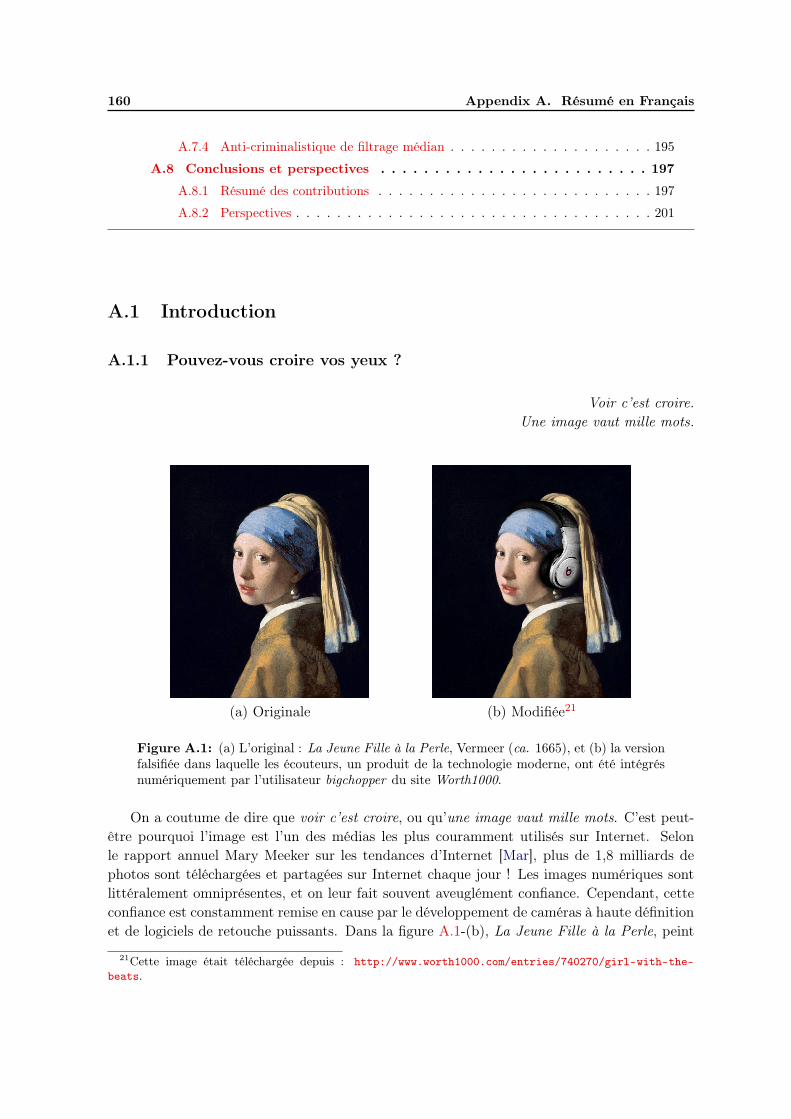
160 Appendix A. Résumé en Français
A.7.4 Anti-criminalistique de filtrage médian . . . . . . . . . . . . . . . . . . . . 195
A.8 Conclusions et perspectives . . . . . . . . . . . . . . . . . . . . . . . . . 197
A.8.1 Résumé des contributions . . . . . . . . . . . . . . . . . . . . . . . . . . . 197
A.8.2 Perspectives . . . . . . . . . . . . . . . . . . . . . . . . . . . . . . . . . . . 201
A.1 Introduction
A.1.1 Pouvez-vous croire vos yeux ?
Voir c’est croire.
Une image vaut mille mots.
(a) Originale (b) Modifiée21
Figure A.1: (a) L’original : La Jeune Fille à la Perle, Vermeer (ca. 1665), et (b) la versionfalsifiée dans laquelle les écouteurs, un produit de la technologie moderne, ont été intégrésnumériquement par l’utilisateur bigchopper du site Worth1000.
On a coutume de dire que voir c’est croire, ou qu’une image vaut mille mots. C’est peut-être pourquoi l’image est l’un des médias les plus couramment utilisés sur Internet. Selonle rapport annuel Mary Meeker sur les tendances d’Internet [Mar], plus de 1,8 milliards dephotos sont téléchargées et partagées sur Internet chaque jour ! Les images numériques sontlittéralement omniprésentes, et on leur fait souvent aveuglément confiance. Cependant, cetteconfiance est constamment remise en cause par le développement de caméras à haute définitionet de logiciels de retouche puissants. Dans la figure A.1-(b), La Jeune Fille à la Perle, peint
21Cette image était téléchargée depuis : http://www.worth1000.com/entries/740270/girl-with-the-
beats.

A.1. Introduction 161
par Johannes Vermeer au XVIIèmes., le personnage semble apprécier la musique provenantd’écouteurs pourtant commercialisés au XXIèmes.
Aujourd’hui encore plus qu’hier, nous avons besoin de voir plus profondément qu’avec nosyeux pour démêler le vrai du faux dans une image.
Créer de fausses images visuellement plausibles est devenu de moins en moins difficile,et notre confiance dans les images numériques est progressivement érodée par le développe-ment des technologies modernes de l’information car des images falsifiées, pouvant facilementtromper les yeux humains, apparaissent de plus en plus fréquemment. Malheureusement, cen’est pas toujours dans un but aussi innocent que le pur amusement visiblement ressenti parl’auteur de la figure A.1-(b). La falsification d’image peut aussi et surtout être malveillante,tant dans la sphère publique que dans la vie privée – et la frontière toujours plus floue entreles deux souligne l’acuité du problème. Fourandsix Technologies, Inc. maintient une galeried’images22, qui recense les faux les plus notables travers l’Histoire. Parmi ces faux, certainsétaient assez dommageables pour causer de sévères pertes financières, ou même impacter néga-tivement l’ensemble de la société.
Le doute qui devrait toujours légitimement entacher les images numériques a donnénaissance à la criminalistique, qui essaye de rétablir une certaine confiance dans les im-ages numériques. Les objectifs principaux de la criminalistique sont d’analyser une imagenumérique de manière à détecter si elle est authentique ou non, d’identifier son origine, deretracer l’histoire des traitements qu’elle a subis, ou de révéler les détails cachés invisibles pourdes yeux humains [Fou].
Au cours de la dernière décennie, les chercheurs ont proposé différentes techniques encriminalistique d’image. Dans un premier temps, le tatouage fragile d’image était le choix leplus populaire pour l’authentification d’image. Dans la littérature, le tatouage fragile est eneffet considéré comme relevant de la criminalistique active [Con11]. Le tatouage intègre lesinformations d’authentification dans l’image quand elle est capturée ou avant sa transmission.Par la suite, l’image peut être authentifiée si le filigrane extrait correspond à celui embarqué.L’image sera considérée comme fausse si l’extraction de filigrane échoue ou si l’informationextraite ne correspond pas à celle qui avait été insérée. Dans ce scénario, un dispositif spé-cial d’acquisition d’image est nécessaire. De fait, l’idée de la caméra de confiance, équipéed’un système de tatouage, a été proposée dès 1993 [Fri93]. Cependant, son déploiement dansl’industrie a rencontré de nombreuses difficultés, qui restent actuellement encore à résoudre.Tout d’abord, il est apparemment difficile pour les différents fabricants d’appareils de prisede vue de parvenir à un accord sur un protocole standard commun. Par ailleurs, les con-sommateurs peuvent trouver qu’il est inacceptable de diminuer la qualité visuelle de l’imagepar l’insertion d’un filigrane. En outre, si le système de tatouage à l’intérieur de la caméradevait un jour être piraté, il deviendrait obsolète du jour au lendemain sans possibilité aiséed’assurer une quelconque rétro-compatibilité avec une nouvelle version corrigeant la faille desécurité. Un exemple de tentative de réalisation de ce type de caméra dans l’industrie estl’Aigo V80PLUS [Aig], commercialisée par Beijing Huaqi Digital Information Technology Co.,
22Disponible à la page http://www.fourandsix.com/photo-tampering-history/.

162 Appendix A. Résumé en Français
Ltd en 2005. Dans cet appareil, un système de filigrane numérique est inclus, qui insère les in-formations d’authentification dans l’image au moment de l’enregistrement. Pourtant, l’usagede la caméra de confiance reste marginal, en raison des préoccupations décrites précédemment.
Conscient des limites de la criminalistique active, les chercheurs tournent progressive-ment leur attention vers la criminalistique passive [Far09a, Con11]. En comparaison avecl’authentification d’image par tatouage fragile, la criminalistique passive vise à évaluer demanière aveugle l’authenticité d’une image donnée, sans aucune autre information a priori
(comme peut par exemple l’être un filigrane). L’hypothèse ici est que si l’on peut facilementcréer de fausses images sans laisser de traces visuelles, la falsification d’image perturbera parcontre très probablement les propriétés statistiques intrinsèques de l’image authentique. Parconséquent, nous choisissons de détecter une manipulation d’image en examinant l’incohérenceou la déviation de statistiques sous-jacentes d’une image. Dans la littérature, la “ criminal-istique passive ” est souvent appelée “ criminalistique ”. Dans la suite de ce document, nousomettrons également l’épithète pour des raisons de concision. De la même manière, nousomettrons souvent le fait qu’il s’agisse ici systématiquement de criminalistique d’image, leséventuelles exceptions seront rendues évidentes par le contexte.
La criminalistique en imagerie numérique est devenue un sujet de recherche important aucours des dernières années. La figure A.2 montre le nombre annuel de publications depuis 2000de l’IEEE [Iee] sur le sujet. Dans cette figure, la barre grise représente les publications avec lemot-clé “ criminalistique ”, alors que la barre hâchurée en gris clair se rapporte aux publicationsavec les mots-clés “ criminalistique ” et “ image ”. Si la criminalistique en général a reçu uneattention croissante dans la dernière décennie, sa spécialisation pour l’image représente à elleseule environ 40% du total.
Year
Number of IEEE publications
0
100
200
300
400
2000
2001
2002
2003
2004
2005
2006
2007
2008
2009
2010
2011
2012
2013
Figure A.2: Nombre annuel de publications de l’IEEE dont mots-clés incluent “ criminal-istique ” (la barre grise), et à la fois “ criminalistique ” et “ image ” (la barre hâchurée engris clair).

A.1. Introduction 163
A.1.2 Anti-criminalistique en images numériques
Les deux faces d’une même pièce.
De même que la cryptographie (resp. la stéganographie) trouve son pendant nécessaireavec la cryptanalyse (resp. la stéganalyse), le “mauvais génie” de la criminalistique est l’anti-criminalistique. L’anti-criminalistique consiste donc en l’étude des limites des méthodescriminalistiques, dans le but ultime de contribuer à leur amélioration [BK13]. À ce titre, cetexercice est primordial et doit guider toute analyse du problème. L’objectif assigné à l’anti-criminalistique est alors d’effectuer un traitement sur l’image falsifiée, spécifiquement destinéà atténuer les traces laissées par la falsification de sorte qu’elle ne sera plus détectée par lesméthodes criminalistiques.
Le développement de la criminalistique en est encore à son stade précoce, et l’anti-criminalistique est un sujet encore plus récent [KB07]. Dans la littérature, les publicationssur la criminalistique sont d’ailleurs beaucoup plus nombreuses que celles relevant de l’anti-criminalistique. En outre, les méthodes anti-criminalistiques actuelles utilisent souvent destraitements simples pour dissimuler les traces laissées par une opération usuelle participantde la falsification, par exemple en utilisant un filtrage ad-hoc pour dissimuler les artefacts decompression JPEG [SL11], ou encore en ajoutant du bruit pour masquer ceux induits plusgénéralement par une opération de filtrage linéaire sur l’image [WSL13]. Il se trouve que cetype de méthodes anti-criminalistique peut réussir à tromper les détecteurs criminalistiquesad-hoc, mais elles peuvent être détectées par des détecteurs plus avancés. Par ailleurs, l’imageanti-criminalistique créée par ces méthodes souffre souvent d’une qualité médiocre. C’est unequestion centrale, car une image de faible qualité (par exemple, une image floue/bruitée) peutspontanément éveiller les soupçons sur son authenticité.
En résumé, l’anti-criminalistique d’image a un double objectif: assurer une bonne in-détectabilité criminalistique, ainsi qu’une haute qualité d’image [KR08]. Si ces deux butsdevenaient antagonistes, le contexte de ce travail imposerait naturellement de privilégierl’indétectabilité sur la qualité.
A.1.3 Objectifs et contributions
Dans cette thèse, nous nous plaçons du côté de l’anti-criminalistique, et nous nous concentronssur la compression JPEG et le filtrage médian. À partir d’une image compressée en JPEGou filtrée par le filtre médian, si nous pouvons réussir à créer une image qui ressemble àcelle non traitée, alors ce sera une tâche relativement facile que de falsifier l’histoire destraitements d’une image, ou même de changer la sémantique portée par l’image. À cettefin, nous employons certains aspects de la restauration d’image, en même temps que nousleur intégrons certains termes/stratégies spécifiquement dédiés à l’anti-criminalistique. Decette façon, nous espérons créer des images anti-criminalistiques avec un bon équilibre entrel’indétectabilité criminalistique et la qualité de l’image falsifiée.

164 Appendix A. Résumé en Français
A.1.3.1 Compression JPEG et filtrage médian
Tout d’abord, nous choisissons de mener nos recherches sur l’anti-criminalistique de compres-
sion JPEG, parce que le format JPEG est probablement le format d’image le plus communen usage aujourd’hui sur Internet, et à ce titre souvent étudié dans de nombreux scénarios encriminalistique. Selon des statistiques sur l’utilisation des formats d’image sur Internet, au 8décembre en 2014, le format JPEG était le plus utilisé, avec une utilisation de 68.7%, toussites confondus [W3t].
Figure A.3: Illustration de créer une image composite en JPEG. Ici, q1, q2 et q3 sont troisprobablement différents facteurs de qualité JPEG.
Pour illustrer l’intérêt d’étudier l’anti-criminalistique JPEG, nous nous appuyons sur lescénario suivant, illustré dans la figure A.3 : afin de faire croire que quelqu’un a participé à uncertain événement, le faussaire créera très probablement une image composite avec la scèneet la victime à partir de deux images JPEG avec différents facteurs de qualité23. L’imagecomposite est enfin compressée en JPEG une dernière fois, avec un autre facteur de qualitéJPEG, pour publication. Une modification habilement effectuée peut ne laisser aucune tracevisible aux yeux humains, mais l’image falsifiée pourrait être confondue par la détection dedifférents artefacts de double compression JPEG présents dans les différentes zones de l’imagecomposite [BP12b].
23Le facteur de qualité JPEG est un nombre entier entre 1 et 100. Plus le facteur de qualité JPEG est élevé,meilleure est la qualité de l’image, et plus la taille du fichier JPEG est grande.
A.1. Introduction 165
D’une manière générale, l’objectif de l’anti-criminalistique JPEG est de supprimer toute
trace éventuelle de compression JPEG, de sorte que l’image JPEG anti-criminalistique a l’aird’une image originale et non compressée. C’est typiquement ce que ferait un faussaire réelle-
ment habile, pour dissimuler au mieux son forfait, juste avant la dernière étape de compressionavant publication [SL11].
Dans des travaux récents d’anti-criminalistique (sur la compression JPEG [SL11] ainsi quesur le rééchantillonnage [KR08]), le filtre médian est utilisé pour masquer efficacement lesdifférentes de traitements effectués sur l’image. Cependant, le filtrage médian, vu comme undébruitage d’image et un opérateur de lissage, laisse des traces dans l’image. Elles peuventêtre détectées par des méthodes criminalistiques de filtrage médian. La présence de tracesde filtrage médian, non seulement donne à penser que l’image a été préalablement filtréepar le filtre médian, mais aussi implique la possibilité que d’autres opérations de traitementd’image ont pu être appliquées à l’image. Par conséquent, il est primordial d’étudier l’anti-
criminalistique du filtrage médian, qui constitue ainsi le second sujet de recherche de cettethèse.
A.1.3.2 Anti-criminalistique d’image et restauration d’image
Dans une certaine mesure, l’anti-criminalistique d’image partage quelques similitudes avecla restauration d’image. En codage ou traitement d’image, leur objectif à tous les deuxconsiste à approcher au mieux les informations perdues pendant le processus de dégradationd’image, souvent en résolvant un problème mal posé. Notons d’emblée que pour certainsscénarios anti-criminalistiques extrêmes (par exemple, la modification du processus physiqueou géométrique [Far09a] de génération de l’image), cette similitude ne tient plus. Néanmoins,l’étude de ces scénarios nous semble relever davantage des effets spéciaux au cinéma, et nousnous concentrons principalement sur la compression JPEG et le filtrage médian. Par rapportà la restauration d’image (et à son seul objectif d’amélioration de la qualité de l’image), l’anti-criminalistique d’image a un autre objectif, encore plus impérieux, i.e. : être indétectable parla criminalistique.
Fondée sur des similitudes entre l’anti-criminalistique et la restauration d’images, cettethèse vise à créer, à partir d’une image compressée en JPEG ou filtrée par le filtre médian,une image “ naturelle ” qui semblera n’avoir jamais été traitée. À cette fin, l’estimateurdu MAP (ou une de ses variantes) sera employé. Nous chercherons donc la meilleure imagefalsifiée, au double sens de l’indétectabilité et de la qualité, et cette recherche, comme il estde mise pour une estimation du MAP dans le cas général, fera intervenir plusieurs méthodesd’optimisation numérique.
A.1.3.3 Méthodologie
À la différence des méthodes anti-criminalistiques de l’état de l’art basées sur le traitementd’image simple [SL11, WSL13], cette thèse propose une nouvelle piste de recherche pour
166 Appendix A. Résumé en Français
falsifier des images. Nous proposons des méthodes anti-criminalistiques sophistiquées visantla compression JPEG et le filtrage médian, en nous appuyant sur des concepts/outils avancésde la restauration d’image, les statistiques d’image naturelle et l’optimisation numérique.
Les effets de bloc dans le domaine spatial et les artefacts de quantification dans le domaineDCT sont deux indices bien connus d’une compression JPEG [FD03]. Dans cette thèse, lesméthodes suivantes sont développées pour l’anti-criminalistique JPEG :
• Tout d’abord, une minimisation contrainte basée sur la variation totale (TV) [ADF05]est employée pour éliminer les effets de bloc de la compression JPEG. En outre, afind’assurer une haute qualité pour l’image falsifiée en bout de chaîne, une projection detype QCS [RS05] est utilisé.
• Pour supprimer les artefacts de quantification dans le domaine DCT, une méthode delissage perceptuel de l’histogramme DCT est proposée, utilisant une loi de Laplace localeet de l’information en partie récupérée dans le domaine DCT par le déblocage TVprécédemment proposé.
• Afin d’étudier l’impact d’un modèle d’image plus avancé que la TV sur l’anti-criminalistique JPEG, nous considérons aussi une mixture de gaussiennes (GMM) pourmodéliser les patchs d’image [ZW11] allié à un terme de vraisemblance modélisant leprocessus de compression JPEG [RS05]. Par ailleurs, nous proposons également unenouvelle méthode non-paramétrique afin de lisser l’histogramme DCT, basée cette foissur le calibrage [FGH02].
Quant à l’anti-criminalistique du filtrage médian, cette thèse propose une déconvolutionvariationnelle d’image, dans une certaine mesure inspiré par [KF09, KTF11]. La fonction decoût de ce problème d’optimisation est composée d’un terme de convolution qui approche leprocessus de filtrage médian, d’un terme de fidélité d’image qui conserve l’image traitée dansune certaine mesure proche de l’image qui a subi le filtrage médian, et d’un terme d’a prioribasé sur une gaussienne généralisée qui régularise la dérivée de l’image obtenue.
Afin de valider l’efficacité des méthodes anti-criminalistiques proposées pour la compressionJPEG et le filtrage médian, nous effectuons des tests à grande échelle. Les méthodes que nousproposons surpassent les méthodes anti-criminalistiques de l’état de l’art, à la fois au regardde leur capacité à résister aux différents criminalistiques simultanément, et de la qualité del’image anti-criminalistique produite.
A.1.4 Organisation du résume
Le reste de ce résumé est organisé de la manière suivante :
La section A.2 introduit quelques notions de base sur la criminalistique et l’anti-criminalistique d’image, y compris la classification, les métriques d’évaluation, les ensembles

A.2. Préliminaires 167
d’image utilisés dans les tests de cette thèse, et les méthodes d’optimisation numérique quiseront utilisées en résolvant les problèmes proposés.
La section A.3 présente les méthodes criminalistiques/anti-criminalistiques dans l’état del’art sur la compression JPEG et le filtrage médian. Les méthodes de criminalistique con-stituent les détecteurs cibles nous attaquerons, alors que les méthodes d’anti-criminalistiqueconstitueront nos concurrents pour les comparaisons expérimentales.
La section A.4 propose une méthode de déblocage de compression JPEG, en optimisantun problème de minimisation contrainte basée sur la TV, dont la fonction de coût est composéd’un terme de TV et d’un terme mesurant le blocage basé sur la TV. Outre un bon effetde déblocage, l’image JPEG anti-criminalistique atteint également une relativement bonneindétectabilité criminalistique, même contre les détecteurs examinant les artefacts de quan-tification. Cependant, ces artefacts de quantification dans le domaine DCT existent, et ilspeuvent potentiellement être utilisés par d’autres détecteurs. Par conséquent, cette méthodesera encore améliorée dans la section A.5.
La section A.5 décrit une méthode améliorée pour l’anti-criminalistique JPEG basée surle travail de la section A.4. Les artefacts de quantification restants dans le domaine DCTaprès le processus de déblocage TV sont explicitement éliminés par une procédure de lissageperceptuel de l’histogramme DCT.
La section A.6 présente une méthode visant à améliorer la qualité de l’image falsifiée, et quidans le cadre du MAP, utilise une GMM pour modéliser les patchs d’image. Afin de produirel’image anti-criminalistique, un lissage de l’histogramme DCT est effectué en utilisant uneméthode non-paramétrique basée sur le calibrage.
La section A.7, cette fois dans le cadre de l’anti-criminalistique du filtrage médian, proposeune déconvolution variationnelle d’image qui modélise la différence de valeurs de pixels enutilisant la loi gaussienne généralisée.
La section A.8 conclut cette thèse, en résumant les contributions et en proposant plusieursdirections de recherche sur la criminalistique et l’anti-criminalistique d’image.
A.2 Préliminaires
A.2.1 Classification de la criminalistique et l’anti-criminalistique d’image
Dans la littérature, il existe différentes taxonomies en criminalistique et en anti-criminalistiqued’image [Far09a, RTD11, Piv13, SWL13, BK13]. Pour la criminalistique d’image, celle pro-posée par Farid [Far09a] est probablement la plus reconnue. La criminalistique d’image faitl’hypothèse que le processus de création de fausses images perturbe certains propriétés intrin-sèques de scène/d’image (par exemple, les propriétés statistiques, physiques ou géométriques).Dans ce contexte, Farid [Far09a] propose de diviser les différentes stratégie de criminalistique
168 Appendix A. Résumé en Français
d’image suivant les cinq catégories suivantes :
• La criminalistique d’image à base de pixels analyse les anomalies causées par la falsifi-cation au niveau du pixel. Les moyens de manipulation d’image fréquemment utiliséssont, par exemple, le copier-coller, l’épissage, le rééchantillonnage, le filtrage médian,etc. Afin de détecter chaque type d’opération sur l’image, de nombreuses méthodescriminalistiques ont déjà été proposées.
• La criminalistique d’image basée sur le format détecte le changement statistique in-troduit par une méthode de compression particulière. Les algorithmes populaires decompression d’image incluent, par exemple, le JPEG basé sur la transformée DCT, leSPIHT et le JPEG2000 basés sur la transformée en ondelettes, etc.
• La criminalistique d’image basée sur la caméra étudie les traces laissées par le dispositifde capture de l’image [Far06]. Les méthodes criminalistiques dans cette catégorie sontbasées, par exemple, sur l’analyse de l’aberration chromatique, du CFA, du PRNU, etc.
• La criminalistique d’image basée sur la physique examine les anomalies de l’interactionentre les différents objets d’une scène, la lumière et la caméra dans le monde physiqueen 3 dimensions. Par exemple, les incohérences de directions de la lumière estimées àpartir de différents objets physiques peuvent être utilisées comme critères aux fins decriminalistique.
• La criminalistique d’image basée sur la géométrie mesure les positions des objetsphysiques par rapport à la caméra. Par exemple, la manipulation d’image peut êtredétectée s’il existe des incohérences au point focal de l’image24.
Pour l’anti-criminalistique d’image, Böhme et Kirchner [BK13] ont divisé les techniques del’anti-criminalistiques d’image en deux grandes catégories, suivant les trois dimensions suiv-antes :
• Robustesse versus sécurité. En toute généralité, les faussaires peuvent exploiter les faib-lesses de robustesse ou de sécurité des méthodes criminalistiques. La robustesse en crim-inalistique désigne la confiance que l’on a dans le diagnostic d’un traitement effectué surl’image, et la sécurité désigne la capacité à détecter comme telles des images falsifiées,même si elles ont fait l’objet d’un traitement anti-criminalistique spécifique. En d’autrestermes, et en réfléchissant au pire des cas comme nous y oblige le principe de Kerckhoffsen sécurité, la sécurité indique la capacité à résister à des attaques anti-criminalistiques.
• Attaques de post-traitement versus traitement intégrés. Les attaques dites de post-
traitement sont une étape de traitement supplémentaire et spécifique dans le processusde falsification, afin qu’il ne reste plus de traces dans l’image qui puissent être détectéespar la criminalistique. Les attaques intégrées, de leur côté, interfèrent directement avecle processus de falsification de l’image. Par définition, ces derniers ne sauraient êtreévalués pertinemment sous l’angle de la robustesse.
24Le point focal est la projection du centre de la caméra sur le plan de l’image.

A.2. Préliminaires 169
• Attaques ciblées versus attaques universelles. Si une méthode anti-criminalistique ex-ploite les faiblesses d’un outil criminalistique spécifique, elle est dite ciblée (ou ad-hoc).Une méthode universelle essaiera quant à elle de créer une image falsifiée dont les pro-priétés statistiques sont maintenues aussi plausibles que possible, de sorte que l’imagefalsifiée reste indétectable, même si elle devait être examinée par des outils criminalis-tiques encore inconnus aujourd’hui.
De la restauration d’image, cette thèse emprunte quelques méthodes d’estimation du MAP(ou une de ses variantes) et intègre certains termes/stratégies anti-criminalistiques. Selon laclassification de Farid [Far09a], la criminalistique JPEG est basée sur le format, alors que lacriminalistique du filtrage médian est à base de pixels. Selon la classification de Böhme etKirchner [BK13], les méthodes anti-criminalistiques proposées à la fois pour la compressionJPEG et le filtrage médian sont des post-traitements de l’image à falsifier, sont ciblées, etpermettent d’analyser la sécurité des méthodes criminalistiques.
A.2.2 Métriques d’évaluation
A.2.2.1 Indétectabilité criminalistique
Comme indiqué dans la section A.1, l’anti-criminalistique d’image a un double objectif : unebonne indétectabilité criminalistique et une haute qualité de l’image anti-criminalistique. Ladétectabilité (pour le côté criminalistique) est une métrique qui n’a de sens qu’en rapportavec l’indétectabilité (pour l’anti-criminalistique). Ces deux métriques sont souvent expriméespar une courbe ROC, qui peut être générée en comparant les performances d’un détecteurcriminalistique avec la vérité terrain, sur un ensemble d’images conséquent. On considèreun ensemble de vraies images (des images originales, les échantillons négatifs) et de faussesimages (des images traitées, les échantillons positifs). Pour chaque stratégie de classificationdu détecteur criminalistique, on peut calculer un taux de vrais positifs et un taux de faux
positifs. Chaque couple de ces deux taux constitue un point de la courbe ROC, dont unexemple est présenté dans la figure A.4.
Pour une évaluation quantitative, nous utilisons la métrique AUC, en mesurant l’aire sousla courbe ROC. La valeur AUC varie dans l’intervalle [0, 1]. Lorsque la valeur AUC est prochede 1, cela signifie que la courbe ROC est proche du point de classification parfaite de l’espaceROC, indiquant une bonne détectabilité criminalistique et une mauvaise indétectabilité crimi-nalistique. Lorsque la valeur AUC est proche de 0.5, cela signifie que la courbe ROC est prochede la ligne de classification aléatoire (à savoir la diagonale de l’espace ROC représentée parla ligne pointillée en rouge dans la figure A.4), indiquant une bonne indétectabilité criminal-istique et une mauvaise détectabilité criminalistique. Lorsque la valeur AUC est proche de 0,cela ne veut pas dire que la détectabilité criminalistique du détecteur est faible, car il suffiraitd’inverser les résultats de classification pour tendre vers 1. En toute généralité, l’objectif del’anti-criminalistique d’image est d’amener la courbe ROC d’un détecteur criminalistique versla ligne de classification aléatoire. Dans ce cas, la valeur AUC est proche de 0.5.

170 Appendix A. Résumé en Français
False positive rate
Truepositive
rate
0 0.2 0.4 0.6 0.8 10
0.2
0.4
0.6
0.8
1
Random guess
Figure A.4: Un exemple de la courbe ROC.
La validation d’un détecteur criminalistique nécessite deux ensembles d’images, des au-thentiques et des fausses, en plus du détecteur à valider. Pour notre procédure de validationcriminalistique, nous utilisons un ensemble d’images originales (cf. la section A.2.3), sur cha-cune desquelles on vient appliquer le traitement à détecter afin de produire l’ensemble despositifs. Le test utilisera donc une quantité égale de positifs et de négatifs.
D’autre part, la caractéristique analysée par un détecteur criminalistique pour prendre sadécision peut être soit un scalaire soit un vecteur, selon la méthode considérée. Lorsque lacaractéristique est un scalaire, on fera varier la valeur du seuil de décision afin de mesurer lecomportement global du détecteur, et lorsque la caractéristique est un vecteur, la littératureretient souvent l’utilisation d’une machine à support vecteur (SVM).
Les détecteurs à base de SVM font l’hypothèse que la méthode anti-criminalistique àdétecter est connue, et que l’on est capable de créer une grande quantité de fausses imagespour l’entraînement du détecteur. Cela correspond à la configuration la plus accomoddantepour la criminalistique, et au pire scénario pour l’anti-criminalistique. Dans la pratique, etdans ce pire des scénarios, nous constatons également qu’il est très difficile de faire passerune image traitée (compressée en JPEG ou filtrée par le filtre médian dans cette thèse) pourune image originale lorsque le détecteur utilise un SVM. Actuellement, aucune méthode anti-criminalistique d’image ne peut tromper les détecteurs puissants à base de SVM.
Inspiré par le scénario de création d’une image composite (illustré dans la figure A.3) et lastéganographie, nous utilisons la configuration expérimentale suivante pour entraîner/testerles détecteurs à base de SVM. Comme illustré dans la figure A.5, pour chaque imageoriginale, la partie centrale de l’image est remplacée par son image traitée correspon-dante (compressée en JPEG ou filtrée par le filtre médian, et avec ou sans l’applicationd’un traitement anti-criminalistique) avec un taux de remplacement prenant les valeurs{0.05, 0.1, 0.15, 0.2, 0.3, 0.4, 0.5, 0.6, 0.8, 1} pour créer les images traitées. Pour chaque taux deremplacement, les fausses images composites et les images originales sont ensuite mélangées en-semble afin de entraîner/tester les détecteurs à base du SVM. Pour le côté anti-criminalistique,

A.2. Préliminaires 171
Figure A.5: Illustration de la création d’une fausse image composite afin d’entraîner/testerun détecteur à base de SVM.
cette thèse considère essentiellement les résultats obtenus avec un taux de remplacement rel-ativement faible. Nous restons réservés sur l’indétectabilité criminalistique d’un traitementappliqué sur la totalité de la surface de l’image originale. Cependant, on peut déjà trouver denombreuses applications dans de nombreux scénarios anti-criminalistiques. Par exemple, uneimage falsifiée peut être créée par le remplacement de la tête d’une personne dans la photo,sans être détectée.
A.2.2.2 Qualité d’image
Les méthodes d’évaluation de la qualité d’image peuvent être groupées en deux catégories: les métriques sans référence et celles avec référence, selon que l’image originale sans dé-formation est connue ou non [WB06]. Dans les scénarios du monde réel, l’image originaleest habituellement inaccessible. Cependant, nous disposons souvent la vérité terrain dansla recherche scientifique. Dans ce cas, l’évaluation de la qualité avec référence est possible.Dans cette thèse, nous ne considérons que les images en niveau de gris 8 bits. Nous utilisonsdeux métriques très connues avec référence pour évaluer la qualité d’image : le PSNR et leSSIM [Wan+04]. L’image originale est utilisée pour calculer les valeurs PSNR et SSIM, afind’évaluer quantitativement la qualité de l’image anti-criminalistique. Plus ces deux valeurssont élevées, plus la qualité de l’image traitée est bonne.
172 Appendix A. Résumé en Français
A.2.2.3 Comparaison d’histogrammes
Souvent, afin de créer l’image anti-criminalistique d’une image compressée en JPEG ou filtréepar le filtre médian, nous sommes amenés à traiter des histogrammes : l’histogramme descoefficients DCT pour la compression JPEG, et l’histogramme des différences de valeurs depixels pour le filtre médian. Afin d’évaluer la restauration de l’histogramme, nous adoptonsla divergence de Kullback-Leibler [KL51] pour mesurer la ressemblance entre l’histogrammede l’image anti-criminalistique et celui de l’image originale. L’objectif du faussaire est dediminuer cette valeur de divergence vers 0.
A.2.3 Ensembles d’images naturelles
Dans la littérature de l’anti-criminalistique de la compression JPEG [Sta+10a, Sta+10b,VTT11, SS11], l’ensemble UCID [SS04] est le plus utilisé. Nous choisissons donc d’utilisercet ensemble d’images. Il contient au total 1338 images de taille 384× 512 et au format TIFFqui n’ont jamais été compressées. Puis ces images en mode RGB sont transformées en niveaude gris à l’aide de la fonction Matlab rgb2gray.
Pour différents usages lors du test de l’anti-criminalistique de la compression JPEG, lesensembles suivants sont créés à partir de l’ensemble UCID :
• UCIDLearn, les 338 dernières images de l’ensemble UCID, pour apprendre un modèled’image et les matrices de covariance du bruit de compression JPEG dans la domainespatial.
• UCIDTest, les 1000 premières images de l’ensemble UCID, pour le test anti-criminalistique en utilisant les détecteurs à base de caractéristique scalaire, et aussipour l’évaluation de la qualité de l’image traitée et de la restauration de l’histogrammeDCT.
– UCIDTR, 500 images choisies de façon aléatoire parmi les images UCIDTest, pourtester les détecteurs à base de SVM.
– UCIDTE, les 500 autres images dans l’ensemble UCIDTest qui ne sont pas choisiespour l’ensemble UCIDTR, pour entraîner les détecteurs à base de SVM.
– UCIDTest92, 92 images choisies de façon aléatoire dans l’ensemble UCIDTest, pourrégler les paramètres de la méthode proposée ou pour analyser rapidement la per-formance de la méthode proposée.
– UCIDTest100, 100 images choisies de façon aléatoire de l’ensemble UCIDTest, pourl’application anti-criminalistique de la double compression JPEG.
Pour le test criminalistique du filtrage médian, les ensembles d’images sont créés à partirde 545 images25 de haute résolution et au format TIFF qui n’ont jamais été compressées, ni
25Ces images peuvent être téléchargées depuis : ftp://firewall.teleco.uvigo.es:27244/DS_01_UTFI.zipet ftp://lesc.dinfo.unifi.it/pub/Public/JPEGloc/dataset/.

A.2. Préliminaires 173
échantillonnées, ni filtrées. Trois images de taille 512 × 512 sont extraites depuis le centrede l’image de haute résolution, puis elles sont transformées en niveaux de gris à l’aide de lafonction Matlab rgb2gray. Les images ainsi extraites qui n’ont pas de valeurs valides pourles algorithmes criminalistiques du filtrage médian [KF10, Cao+10, Yua11] sont exclues. In
fine, nous avons au total 1607 images qui sont ensuite divisées en trois ensembles : le MFTR,le MFTE et le MFPE. En résumé, les quatre ensembles d’images suivants sont utilisés dansles tests criminalistiques dans notre travail sur le filtrage médian :
• MFTR, 500 images pour entraîner les détecteurs criminalistiques à base de SVM.
• MFTE, 1000 images pour le test criminalistique en utilisant les détecteurs basés sur lacriminalistique scalaire et ceux à base de SVM, et aussi pour l’évaluation de la qualitéde l’image traitée et de la restauration de l’histogramme des différences de valeurs depixels.
• MFPE, 107 images pour l’estimation des paramètres.
• MFTE100, 100 images choisies de façon aléatoire dans l’ensemble MFTE, pour réglerles paramètres de la méthode proposée.
A.2.4 Algorithmes pertinents d’optimisation
Pour toutes les méthodes anti-criminalistiques proposées dans cette thèse, plusieurs méthodesd’optimisation numérique sont utilisées de manière à estimer l’image traitée “ la meilleure ”dans un certain sens. Plus précisément, nous utiliserons la méthode de sous-gradient [BXM03],l’algorithme des Hongrois [Kuh55], et le “ Half Quadratic Splitting ” [GY95] et la méthodedite split Bregman [GO09].
La méthode de sous-gradient, itérative, résout un problème de minimisation convexe, selonun sous-gradient de la solution actuelle [BXM03]. Une extension importante de la méthodede sous-gradient est la méthode de sous-gradient projeté, qui permet de résoudre des prob-lèmes d’optimisation sous contraintes. Nous utiliserons la méthode de sous-gradient dans lessections A.4, A.5 et A.6. L’algorithme des Hongrois [Kuh55] est une méthode d’optimisationdiscrète bien connue pour résoudre le problème d’affectation en temps polynomial, cubique.Cette méthode sera utilisée pour résoudre un problème de mise en correspondance des co-efficients DCT pour lisser perceptuellement l’histogramme DCT dans la section A.5. Denombreux problèmes avec régularisation en traitement d’image sont difficiles car souvent non-convexes. Le “ Half Quadratic Splitting ” et la méthode split Bregman ont donc été proposéspour faciliter la résolution de ce type de problème d’optimisation complexe, en divisant leproblème initial en deux sous-problèmes plus simples [GY95, GO09]. Ces deux techniquesd’optimisation seront utilisées dans la sections A.6 et A.7.

174 Appendix A. Résumé en Français
A.3 État de l’art en (anti-)criminalistique de compressionJPEG et de filtrage médian
(a) (b)
DCT coefficient value
DCT
coeffi
cientfrequency
−300 −100 100 3000
0.02
0.04
0.06
(c)
DCT coefficient value
DCT
coeffi
cientfrequency
−300 −100 100 3000
0.2
0.4
0.6
0.8
(d)
Figure A.6: Exemples de les artefacts de la compression JPEG. Ici, l’image JPEG estcompressée de l’image “ Lena ” avec le facteur de qualité JPEG 10.
A.3.1 (Anti-)Criminalistique de compression JPEG
Après une compression JPEG, deux types bien connus d’artefacts apparaissent, trahissantl’histoire de compression JPEG d’une image. Ce sont, respectivement, les effets de bloc dansle domaine spatial, et les artefacts de quantification dans le domaine DCT [FD03]. Un ex-emple d’effet de bloc peut être trouvé dans la figure A.6-(b), en comparant à -(a). Ceci estprincipalement à cause de ce que la compression JPEG traite individuellement chaque blocde taille 8× 8. La présence d’effet de bloc est également liée à la base de la DCT [RS05]. Unexemple des artefacts de quantification peut être trouvé dans la figure A.6-(d), en comparant

A.3. État de l’art en (anti-)criminalistique de compression JPEG et de filtrage médian175
à -(c). Ceci est à cause de ce que la quantification de compression JPEG est conduite dans ledomaine DCT. Afin de créer l’image anti-criminalistique d’une image compressée en JPEG, ilest important d’éliminer ces deux types d’artefacts JPEG.
Table A.1: Détecteurs criminalistiques de compression JPEG.
KQF Détecteur criminalistique basé sur l’estimation de la matrice
de quantification, proposé par Fan et De Queiroz [FD03] ;
KF Détecteur criminalistique basé sur l’analyse des effets debloc, proposé par Fan et De Queiroz [FD03] ;
KLuo Détecteur criminalistique JPEG proposé par Luo et al.[LHQ10] ;
KQLuo Détecteur criminalistique basé sur l’estimation du pas de
quantification, proposé par Luo et al. [LHQ10] ;
KV Détecteur criminalistique basé sur la TV, proposé parValenzise et al. [Val+11, VTT13] ;
KL Détecteur criminalistique basé sur le calibrage, proposé parLai et Böhme [LB11] ;
K1U ,K
2U Deux détecteurs proposés par nous et basés sur l’analyse des
effets de bloc ;
KS100Li Détecteur criminalistique basé sur une caractéristique en 100
dimensions qui exploite la corrélation inter- ou intra-bloc[CS08], proposé par Li et al. [LLH12] ;
KS686P Détecteur criminalistique basé sur la caractéristique SPAM
en 686 dimensions, proposé par Pevný et al. [PBF10].
Table A.2: Notations pour l’image originale, compressée JPEG, et anti-criminalistiquedans l’état de l’art.
I L’image originale, qui n’a jamais été compressée ;
J L’image JPEG, composée à partir de l’image originale I ;
FJSq
L’image anti-criminalistique, créée à partir de l’image JPEG J , parun procédé de tramage, proposé par Stamm et al. [Sta+10a, SL11] ;
FJSqSb
L’image anti-criminalistique, créée à partir de l’image FJSq
, par unprocédé de déblocage basé sur le filtrage médian, proposé par Stammet al. [Sta+10b, SL11] ;
FJV L’image anti-criminalistique, créée à partir de l’image JPEG J , par
un procédé de tramage perceptif, proposé par Valenzise et al.[VTT11] ;
FJSu L’image anti-criminalistique, créée à partir de l’image JPEG J , par
une attaque de SAZ, proposé par Sutthiwan et Shi [SS11].
Les détecteurs de compression JPEG utilisés dans cette thèse sont listés dans la table A.1.Parmi tous les détecteurs de compression JPEG en considération, nous en introduisons unnouveau : Kp
U (avec les paramètres p = 1, et p = 2) qui se fonde sur l’analyse des effets

176 Appendix A. Résumé en Français
de bloc. Les autres sont les détecteurs classiques dans la littérature de la criminalistiqueen compression JPEG. Dans la table A.1, les huit premiers détecteurs sont basés sur descaractéristiques scalaires, alors que les deux derniers utilisent un SVM. Les méthodes anti-criminalistiques en JPEG de l’état de l’art sont listées dans la table A.2. Elles nous serontutiles pour comparer les performances des méthodes que nous proposons.
A.3.2 (Anti-)Criminalistique du filtrage médian
Pixel value difference
Frequen
cy
−300 −100 100 3000
0.1
0.2
0.3
(a) Image originale
Pixel value difference
Frequen
cy
−300 −100 100 3000
0.1
0.2
0.3
(b) MFI
Figure A.7: Exemples de l’histogramme de différence de valeurs de pixels au premier ordrede l’image originale et celui de l’image MF, respectivement.
Pour des raisons de concision, l’abréviation “ MFI ” désigne dans cette thèse l’image quia été filtrée par le filtre médian. La fenêtre du filtre médian peut avoir de nombreuses formeset tailles différentes. Cette thèse utilise la fenêtre carrée de taille 3× 3, qui est aussi la valeurretenue dans l’état de l’art [FB12, WSL13, DN+13]. Dans un certain voisinage de la MFI,la probabilité que les valeurs de pixels proviennent des mêmes pixels de l’image originale estélevée. Cet effet est connu sous le nom d’artefact dit de “ streaking ” [Bov87]. Les artefactsstreaking peuvent également se refléter dans la modification de la forme de l’histogramme desdifférences des valeurs de pixels après filtrage médian. En comparant la figure A.7-(b) avec-(a), on peut voir que le pic autour la classe 0 de différence de valeurs de pixels au premierordre devient plus haut après que l’image est filtrée par le filtre médian.
Dans cette thèse, les détecteurs de l’état de l’art relatifs au filtrage médian sont listés dansla table A.3. Dans cette table, les quatre premiers détecteurs sont basés sur des caractéristiquesscalaires, alors que les cinq derniers utilisent un SVM. Les méthodes anti-criminalistiques del’état de l’art pour le filtre médian sont listées dans la table A.4. Elles seront utilisées pour lacomparaison expérimentale avec les nôtres.

A.4. Anti-criminalistique de compression JPEG basée sur la TV 177
Table A.3: Détecteurs criminalistiques du filtrage médian.
KK Détecteur basé sur l’analyse de la différence de valeurs depixels au premier ordre, proposé par Kirchner et Fridrich[KF10] ;
KK Version améliorée de KK [KF10] ;
KC Détecteur basé sur l’analyse de la différence des valeurs depixels au premier ordre, proposé par Cao et al. [Cao+10] ;
KY Détecteur basé sur une caractéristique fusionnée, proposé parYuan [Yua11] ;
KS686SPAM Détecteur criminalistique basé sur la caractéristique SPAM en
686 dimensions, proposé par Pevný et al. [PBF10];
KS44MFF Détecteur criminalistique basé sur la caractéristique MFF en
44 dimensions, proposé par Yuan [Yua11] ;
KS56GLF Détecteur criminalistique basé sur la caractéristique GLF en
56 dimensions, proposé par Chen et al. [Che+12, CNH13] ;
KS10AR Détecteur criminalistique basé sur la caractéristique MFRAR
en 10 dimensions, proposé par Kang et al. [Kan+12, Kan+13];
KS220LTP Détecteur criminalistique basé sur la caractéristique MFLTP
en 220 dimensions, proposé par Zhang et al. [Zha+14].
Table A.4: Notations pour l’image originale, filtrée médian, et anti-criminalistique dansl’état de l’art.
I L’image originale ;
M L’image filtrée à partir de l’image originale I par le filtre médian,aussi appelée MFI dans le texte ;
FMW L’image anti-criminalistique, créée à partir de la MFI M, par un
procédé de tramage, proposé par Wu et al. [Sta+10b, SL11] ;
FMD L’image anti-criminalistique, créée à partir de la MFI M, par une
injection de bruit, proposé par Dang-Nguyen et al. [DN+13].
A.4 Anti-criminalistique de compression JPEG basée sur la TV
A.4.1 Introduction et motivation
Afin de créer l’image anti-criminalistique d’une image JPEG, il faut supprimer les deux typesd’artefacts présents à la fois dans le domaine DCT et dans le domaine spatial. Dans lapratique, nous trouvons qu’il est extrêmement difficile de mener une attaque en une seuleétape pour tromper plusieurs détecteurs criminalistiques qui travaillent dans deux différentsdomaines, tout en conservant une haute qualité d’image anti-criminalistique. Par conséquent,cette thèse supprime les artefacts JPEG alternativement dans le domaine DCT et dans le

178 Appendix A. Résumé en Français
domaine spatial. Dans cette section, nous nous concentrons sur la suppression des effetsde bloc d’une image JPEG au niveau anti-criminalistique. Nous laissons la suppression desartefacts de quantification dans le domaine DCT suppression pour la section A.5.
Suivant la piste de recherche décrite dans la section A.1.3.3 et visant à utiliser les conceptsde la restauration, cette section présente notre méthode pour supprimer les effets de bloc d’uneimage JPEG (basée sur la régularisation de la TV). L’idée de régulariser de la TV (variationtotale) a été proposé par Rudin et al. [ROF92] en 1992. Depuis lors, elle a été largementutilisée dans la restauration d’image, pour de nombreuses applications comme la réduction dubruit, la déconvolution, l’inpainting, etc. Les effets de bloc conduisent à une valeur plutôt hautede la TV. Par conséquent, le déblocage JPEG peut être effectué en minimisant une fonctiond’énergie basée sur la TV [ADF05]. Traditionnellement, son objectif principal est d’améliorerla qualité de l’image JPEG, mais cela ne suffit pas pour obtenir une bonne indétectabilitécriminalistique. Aux fins de criminalistique, nous ajoutons à la fonction de minimisation unautre terme de mesure du blocage JPEG basé sur la TV. En résolvant un nouveau problème deminimisation basé sur la TV, nous pouvons créer l’image anti-criminalistique avec une bonneindétectabilité criminalistique en sacrifiant un tout petit peu de la qualité d’image.
A.4.2 Déblocage JPEG en minimisant un problème contraint basé sur laTV
Pour image U de la taille H ×W , nous définissons le terme de TV comme :
TVb(U) =∑
1≤i≤H,1≤j≤W
νi,j , (A.1)
avec la variation à l’emplacement de (i, j) :
νi,j =√
(Ui−1,j +Ui+1,j − 2Ui,j)2 + (Ui,j−1 +Ui,j+1 − 2Ui,j)2, (A.2)
où Ui,j est la valeur du (i, j)-ème pixel de l’image U.
Afin d’éliminer les effets de bloc, nous définissons un second terme qui mesure le blocageJPEG. L’idée est très simple : s’il n’y a pas de compression JPEG, statistiquement la sommede l’énergie de la variation des pixels près des frontières du bloc devrait être proche de celledans le centre du bloc. Nous divisons donc tous les pixels de l’image en deux groupes : A etB, en fonction de leur position dans le bloc, comme il est illustré dans la figure A.8. Seloncette classification des pixels, le second terme de l’énergie est défini comme :
C(U) =
∣
∣
∣
∣
∣
∣
∑
Ui,j∈A
νi,j −∑
Ui,j∈B
νi,j
∣
∣
∣
∣
∣
∣
. (A.3)
Le problème contraint final basé sur la TV est composé d’un terme de TV et d’un terme
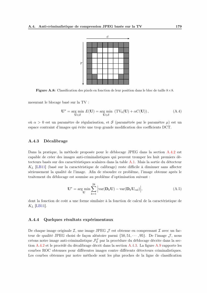
A.4. Anti-criminalistique de compression JPEG basée sur la TV 179
Figure A.8: Classification des pixels en fonction de leur position dans le bloc de taille 8×8.
mesurant le blocage basé sur la TV :
U∗ = arg minU∈S
E(U) = arg minU∈S
(TVb(U) + αC(U)) , (A.4)
où α > 0 est un paramètre de régularisation, et S (paramétrée par le paramètre µ) est unespace contraint d’images qui évite une trop grande modification des coefficients DCT.
A.4.3 Décalibrage
Dans la pratique, la méthode proposée pour le déblocage JPEG dans la section A.4.2 estcapable de créer des images anti-criminalistiques qui peuvent tromper les huit premiers dé-tecteurs basés sur des caractéristiques scalaires dans la table A.1. Mais la sortie du détecteurKL [LB11] (basé sur la caractéristique de calibrage) reste difficile à diminuer sans affectersérieusement la qualité de l’image. Afin de résoudre ce problème, l’image obtenue après letraitement du déblocage est soumise au problème d’optimisation suivant :
U∗ = arg minU
28∑
k=1
∣
∣
∣var(DkU)− var(DkUcal)∣
∣
∣, (A.5)
dont la fonction de coût a une forme similaire à la fonction de calcul de la caractéristique deKL [LB11].
A.4.4 Quelques résultats expérimentaux
De chaque image originale I, une image JPEG J est obtenue en compressant I avec un fac-teur de qualité JPEG choisi de façon aléatoire parmi {50, 51, · · · , 95}. De l’image J , nouscréons notre image anti-criminalistique FJ
0 par la procédure du déblocage décrite dans la sec-tion A.4.2 et le procédé du décalibrage décrit dans la section A.4.3. La figure A.9 rapporte lescourbes ROC obtenues pour différentes images contre différents détecteurs criminalistiques.Les courbes obtenues par notre méthode sont les plus proches de la ligne de classification
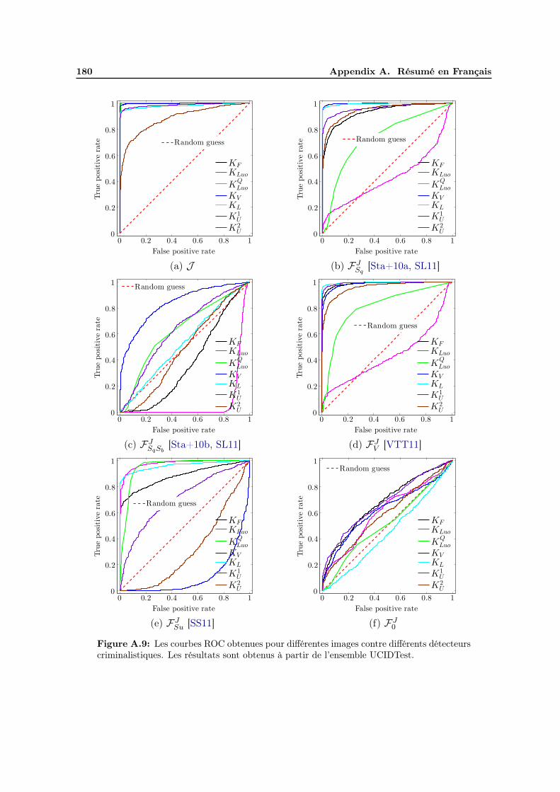
180 Appendix A. Résumé en Français
False positive rate
Truepositiverate
0 0.2 0.4 0.6 0.8 10
0.2
0.4
0.6
0.8
1
KF
KLuo
KQLuo
KV
KL
K1U
K2U
Random guess
(a) JFalse positive rate
Truepositiverate
0 0.2 0.4 0.6 0.8 10
0.2
0.4
0.6
0.8
1
KF
KLuo
KQLuo
KV
KL
K1U
K2U
Random guess
(b) FJSq
[Sta+10a, SL11]
False positive rate
Truepositiverate
0 0.2 0.4 0.6 0.8 10
0.2
0.4
0.6
0.8
1
KF
KLuo
KQLuo
KV
KL
K1U
K2U
Random guess
(c) FJSqSb
[Sta+10b, SL11]
False positive rate
Truepositiverate
0 0.2 0.4 0.6 0.8 10
0.2
0.4
0.6
0.8
1
KF
KLuo
KQLuo
KV
KL
K1U
K2U
Random guess
(d) FJV [VTT11]
False positive rate
Truepositiverate
0 0.2 0.4 0.6 0.8 10
0.2
0.4
0.6
0.8
1
KF
KLuo
KQLuo
KV
KL
K1U
K2U
Random guess
(e) FJSu [SS11]
False positive rate
Truepositiverate
0 0.2 0.4 0.6 0.8 10
0.2
0.4
0.6
0.8
1
KF
KLuo
KQLuo
KV
KL
K1U
K2U
Random guess
(f) FJ0
Figure A.9: Les courbes ROC obtenues pour différentes images contre différents détecteurscriminalistiques. Les résultats sont obtenus à partir de l’ensemble UCIDTest.

A.5. Anti-criminalistique de compression JPEG avec un lissage perceptuel del’histogramme DCT 181
Table A.5: La comparaison de la qualité d’image, où les valeurs PSNR/SSIM sont calculéesavec I comme référence. Les résultats sont obtenus à partir de l’ensemble UCIDTest.
J FJSq
FJSqSb
FJV FJ
Su FJ0
PSNR 37.0999 33.4061 30.4591 33.2890 31.6552 35.4814
SSIM 0.9919 0.9756 0.9509 0.9802 0.9719 0.9843
aléatoire, en comparant avec les méthodes anti-criminalistique de l’état de l’art. La compara-ison de la qualité d’image est explicitée dans la table A.5. La qualité de FJ
0 est la meilleureparmi toutes les images anti-criminalistiques. De ces résultats, on peut conclure que la méth-ode proposée surpasse les méthodes anti-criminalistiques de l’état de l’art [Sta+10a, Sta+10b,SL11, VTT11, SS11], au regard tant de la capacité à résister à la détection des méthodescriminalistiques, que de la qualité de l’image anti-criminalistique produite.
A.5 Anti-criminalistique de compression JPEG avec un lissageperceptuel de l’histogramme DCT
A.5.1 Introduction et motivation
DCT coefficient value
DCTcoeffi
cientfrequency
−100 −50 0 50 1000
0.02
0.04
0.06
0.08
(a) FJSqSb
[Sta+10b, Sta+10a, SL11]DCT coefficient value
DCTcoeffi
cientfrequency
−150 −100 −50 0 50 100 1500
0.04
0.08
0.12
(b) FJ0
Figure A.10: Exemples d’histogrammes DCT de la sous-bande (4, 4), de FJSqSb
[Sta+10a,
Sta+10b, SL11] et de FJ0 , respectivement.
La figure A.10 compare un exemple de l’histogramme DCT de l’image anti-criminalistiqueFJSqSb
[Sta+10b, Sta+10a, SL11] et celui de notre image anti-criminalistique FJ0 créée par la
méthode décrite dans la section A.4. On peut voir que les artefacts de quantification dans ledomaine DCT persistent encore, dans une certaine mesure, dans FJ
0 , généralement dans lessous-bandes de fréquence moyenne de l’image. Cette faiblesse peut potentiellement être utiliséepar les détecteurs criminalistiques avancés. Afin de résoudre ce problème, dans notre seconde

182 Appendix A. Résumé en Français
méthode proposée pour l’anti-criminalistique d’image de compression JPEG, une procédurede lissage perceptuel de l’histogramme DCT est mis au point. Ce lissage d’histogramme estestiné à éliminer les artefacts de quantification restants dans l’image traitée par la méthodede déblocage (mais avec un paramètre différent par rapport à la génération de FJ
0 ).
first-round TV-based deblocking
perceptual DCT histogram smoothing
second-round TV-based deblocking
de-calibration
Figure A.11: Le processus proposé pour créer l’image anti-criminalistique FJ .
À titre d’amélioration de la méthode dans la section A.4, nous proposons une méthode enquatre étapes pour créer l’image anti-criminalistique de l’image JPEG, comme illustré dansla figure A.11 et résumées dans ce qui suit :
• La première étape est le déblocage JPEG en minimisant un problème contraint basésur la TV dans le domain spatial. Cette méthode est identique à celle décrite dansla section A.4.2, mais avec différents paramètres. Après cette étape, l’image générée àpartir de l’image JPEG J est dénotée par FJ
b .
• Les artefacts de quantification dans l’image FJb ne sont plus aussi évidents que ceux
présents dans l’image JPEG J . Sous l’hypothèse que les informations DCT récupéréesen partie sont fiables, la prochaine étape sera naturellement de remplir les vides restantsdans l’histogramme DCT. Cette tâche est remplie par la procédure de lissage perceptuelde l’histogramme DCT, qui sera décrite dans la section A.5.2. FJ
bq désigne l’image
intermédiaire créée à partir de FJb pour cette étape.
• Dans le domaine spatial, afin de supprimer le bruit anormal introduit par la secondeétape, on effectue un second déblocage JPEG. L’image intermédiaire résultante est notéeFJbqb.
• Enfin, l’image FJbqb est traitée par le décalibrage, qui est identique à celui décrit dans la
section A.4.3, afin de générer notre image anti-criminalistique finale FJ .

A.5. Anti-criminalistique de compression JPEG avec un lissage perceptuel del’histogramme DCT 183
Les méthodes dans les première, troisième, et dernière étapes dans la figure A.11 sontdécrites dans les sections A.4.2 et A.4.3, mais avec différents paramètres. Pour le premierdéblocage JPEG, le paramétrage suivant est utilisé : α = 1.5, µ = 0.5 et tk = 1/k (k =
1, 2, · · · , 50). Pour le deuxième déblocage JPEG, le paramétrage suivant est utilisé : α = 0.9,µ = 1.5 et tk = 1/(k+1) (k = 1, 2, · · · , 30). La section A.5.2 présentera la méthode permettantde lisser perceptuellement l’histogramme DCT de l’image FJ
b dans la deuxième étape de lafigure A.11.
A.5.2 Lissage perceptuel de l’histogramme DCT
Afin de lisser l’histogramme DCT, il est important de trouver un bon modèle pour les coeffi-cients DCT. Dans la littérature, la loi de Laplace est un choix très populaire. Son kurtosis vaut6. Nous avons calculé le kurtosis pour chaque sous-bande AC de chaque image de l’ensembleUCID [SS04]. La valeur moyenne est 19.99, qui est beaucoup plus grand que 6, et qui indiqueque la distribution réelle des coefficients DCT a généralement un pic beaucoup plus élevé quela loi de Laplace. D’autre part, 93.68% des valeurs de kurtosis calculés song plus grandes que6. Ces chiffres montrent que la loi de Laplace n’est peut-être pas très appropriée pour mod-éliser les coefficients DCT (un exemple peut être trouvé dans la figure A.12-(a)). En outre,Robertson et Stevenson [RS05] ont souligné que la loi de Laplace fonctionne effectivement bienpour la classe de quantification 0, mais la loi uniforme est un modèle plus approprié pour lesautres classes de quantification.
Sur la figure A.12-(c), on peut voir que les informations dans le domaine DCT sontrécupérées en partie par le premier déblocage JPEG. Mais les artefacts de quantificationpersistent encore, dans un certain mesure, dans FJ
b . Avec ces informations DCT récupérées,et d’après l’analyse ci-dessus, nous proposons un modèle adaptatif local laplacien afin demodéliser les coefficients DCT. L’idée principale est de rechercher le paramètre λb de la loide Laplace pour chaque classe de quantification b, dès la classe 0, en résolvant le problèmecontraint des moindres carrés pondérés suivant :
λb = arg minλ−
b≤λ≤λ+
b
B+r,cQr,c+⌊
Qr,c
2⌋
∑
k=B−
r,cQr,c−⌊Qr,c
2⌋
wk ×(
HUr,c(k)− P (Y = k)
)2, (A.6)
où Qr,c est le pas de quantification pour la sous-bande AC actuelle, B−r,c (resp. B+
r,c) est laclasse de quantification non vide avec la valeur la plus petite (resp. grande) au centre dela classe, wk est le poids, HU
r,c est l’histogramme DCT normalisé, et P est la loi discrète deLaplace. On peut voir ce problème comme celui d’un ajustement local des coefficients DCTpour chaque classe de quantification b. Si un valeur valide est trouvée λb, la loi de Laplacesera utilisée par la classe b. Sinon, c’est la loi uniforme qui sera utilisée pour la classe actuelleb et les suivantes. Pour la sous-bande DC, la loi de Laplace est utilisée pour toutes les classesde quantification.
En construisant le modèle adaptatif de Laplace local comme décrit ci-dessus, on peutobtenir la distribution cible pour les coefficients DCT de chaque sous-bande de l’image. Un

184 Appendix A. Résumé en Français
DCT coefficient value
DCT
coeffi
cientfrequency
−150 −100 −50 0 50 100 1500
0.04
0.08
0.12
0.16
(a)
DCT coefficient value
DCT
coeffi
cientfrequency
−150 −100 −50 0 50 100 1500
0.2
0.4
0.6
(b)
DCT coefficient value
DCT
coeffi
cientfrequency
−150 −100 −50 0 50 100 1500
0.04
0.08
0.12
0.16
(c)
DCT coefficient value
DCT
coeffi
cientfrequency
−150 −100 −50 0 50 100 1500
0.02
0.04
0.06
0.08
0.1
(d)
Figure A.12: (a) est un histogramme DCT de la sous-bande (2, 2) d’une image originale del’ensemble UCID [SS04], et la courbe en rouge est le résultat d’ajustement en utilisant la loidiscrète de Laplace. Cette image est ensuite compressée avec un certain facteur de qualitéJPEG 50 afin de générer l’image JPEG, elle est ensuite traitée par la méthode proposée.(b), (c), et (d) sont les histogrammes correspondants à l’histogramme (a) de l’image JPEGJ , de l’image FJ
b obtenue à partir de J par le premier déblocage JPEG, et d’image obtenue
à partir de FJb par l’injection du signal de tramage local adaptatif, respectivement.
exemple est montré dans la figure A.12-(d). L’histogramme DCT apparaît bien lissé. Àprésent, nous décrivons comment modifier les coefficients DCT afin que leur distribution ap-proche la distribution cible (cf. figure A.12-(d)) et tout en minimsant la distorsion infligéeà l’image par ce traitement précis. Pour ce problème, nous nous proposons un problèmed’affectation et souhaitons trouver une bijection f : Ob → T b de sorte que la fonction de coût:
∑
o∈Ob
W (o, f(o)), (A.7)
soit minimisée. Ici, pour chaque classe de quantification b, Ob est l’ensemble coefficientsDCT originaux, et T b est celui des valeurs cible des coefficient DCT. La fonction de poidsW : Ob × T b → R est définie comme la perte de valeur SSIM à cause de la modification descoefficients DCT. Après la résolution d’un problème d’affectation simplifiée pour chaque classe

A.5. Anti-criminalistique de compression JPEG avec un lissage perceptuel del’histogramme DCT 185
de quantification, nous pouvons lisser l’histogramme DCT perceptuellement avec un minimumde distorsion introduite dans le domaine spatial, puis enfin créer l’image FJ
bq.
A.5.3 Quelques résultats expérimentaux
A.5.3.1 Comparaison de différentes méthodes de tramage
Nous comparons notre méthode de tramage basée sur le modèle adaptatif local de Laplaceavec celle basée sur la loi de Laplace proposée par Stamm et al. [Sta+10a, SL11]. La table A.6rapporte la différence entre la divergence K-L obtenue par FJ
Sq[Sta+10a, SL11] et celle obtenue
par FJbq. Toutes les valeurs de différence listées dans la table A.6 indiquent que la méthode
proposée surpasse constamment la méthode de Stamm et al. [Sta+10a, SL11] pour toutes lessous-bandes DCT
Table A.6: La différence entre la divergence K-L obtenue par FJSq
[Sta+10a, SL11] et
celle obtenue par FJbq pour les 64 sous-bandes DCT. La valeur moyenne de la différence est
0.0552 avec une déviation standard 0.0249. Pour une comparaison équitable avec FJSq
, lessous-bandes dont les coefficients DCT sont tous quantifiés à 0 dans l’image JPEG J , nesont pas comptés. Les résultat sont obtenus à partir de l’ensemble UCIDTest.
rc 1 2 3 4 5 6 7 8
1 0.0001 0.0065 0.0118 0.0278 0.0493 0.0634 0.0663 0.0656
2 0.0042 0.0166 0.0229 0.0363 0.0447 0.0565 0.0504 0.0369
3 0.0161 0.0208 0.0291 0.0442 0.0573 0.0665 0.0634 0.0497
4 0.0200 0.0317 0.0409 0.0470 0.0658 0.0802 0.0553 0.0446
5 0.0357 0.0395 0.0522 0.0678 0.0764 0.0930 0.0927 0.0856
6 0.0441 0.0383 0.0642 0.0610 0.0726 0.0769 0.0806 0.0957
7 0.0538 0.0442 0.0678 0.0595 0.0879 0.0809 0.0948 0.0975
8 0.0619 0.0545 0.0697 0.0528 0.0927 0.0880 0.0854 0.0722
A.5.3.2 Contrer les détecteurs criminalistiques de compression JPEG
Partant d’une image JPEG J , nous la traitons suivant les quatre étapes de la méthode anti-criminalistique proposée (cf. figure A.11) afin de créer l’image anti-criminalistique FJ . Lafigure A.13 montre les courbes ROC obtenues par FJ contre des détecteurs scalaires basés,qui sont toutes proches de la ligne de classificateur aléatoire. Cela signifie que l’image anti-criminalistique créée par la méthode proposée est capable d’atteindre une bonne indétectabilitécriminalistique. Cette information se reflète aussi par les valeurs AUC atteintes par FJ (cf.table A.7), en comparant aux autres méthodes de l’état de l’art. En outre, FJ est capabled’atteindre des valeurs AUC plus petites que les autres images anti-criminalistiques de l’état del’art en variant le taux de remplacement d’image. Selon les résultats de la figure A.14, quand le

186 Appendix A. Résumé en Français
Table A.7: De la deuxième colonne à la huitième colonne, sont listées les valeurs AUCobtenues pour différentes images contre des détecteurs scalaires ; la comparaison de la qualitéd’image (avec I comme référence) est rapportée dans les deux dernières colonnes. Lesrésultats sont obtenus à partir de l’ensemble UCIDTest.
KF KLuo KQLuo KV KL K1
U K2U PSNR SSIM
J 0.9991 1.0000 0.9996 0.9976 0.9811 0.9860 0.8840 37.0999 0.9919
FJSq
0.9332 0.4328 0.7328 0.9977 0.9946 0.9633 0.9483 33.4061 0.9756
FJSqSb
0.3783 0.0806 0.6288 0.8337 0.5338 0.6309 0.4854 30.4591 0.9509
FJV 0.9889 0.4330 0.8066 0.9834 0.9958 0.9916 0.9574 33.2890 0.9802
FJSu 0.8802 0.9772 0.9475 0.1115 0.9610 0.7052 0.3149 31.6552 0.9719
FJ0 0.6756 0.6046 0.5194 0.6210 0.4490 0.6772 0.5880 35.4814 0.9843
FJb 0.7590 0.4830 0.4354 0.8542 0.9588 0.6813 0.5650 36.7405 0.9891
FJbq 0.9170 0.4050 0.5244 0.8435 0.9874 0.8081 0.6531 35.9926 0.9872
FJ 0.5398 0.6425 0.4598 0.6159 0.4344 0.5894 0.5317 35.9855 0.9866
False positive rate
Truepositiverate
0 0.2 0.4 0.6 0.8 10
0.2
0.4
0.6
0.8
1
KF
KLuo
KQLuo
KV
KL
K1U
K2U
Random guess
(b) FJ
Figure A.13: Les courbes ROC obtenues par FJ contre des détecteurs criminalistiques.Les résultat sont obtenus à partir de l’ensemble UCIDTest.
taux de replacement est relativement petit, notre image anti-criminalistique reste indétectablecontre les deux détecteurs à base de SVM [LLH12, PBF10]. De plus, FJ surpasse les autresimages anti-criminalistiques au point de vue de la qualité de l’image, en l’évaluant cette qualitétant par le PSNR que par le SSIM.
Par rapport à la méthode proposée dans la section A.4, le lissage perceptuel d’histogrammeDCT remplit explicitement les lacunes dans l’histogramme DCT de l’image JPEG. Cela aug-mente la performance anti-criminalistique de FJ . Enfin, FJ présente également une meilleurequalité d’image que FJ
0 .

A.6. Amélioration de qualité et anti-criminalistique de l’image JPEG basée sur unmodèle d’image avancé 187
Replacement rate
AUC
0 0.1 0.2 0.3 0.4 0.5 0.6 0.8 10.5
0.6
0.7
0.8
0.9
1
J
FJSq
FJSqSb
FJV
FJSu
FJ0
FJ
(a) KS100Li [CS08, LLH12]
Replacement rate
AUC
0 0.1 0.2 0.3 0.4 0.5 0.6 0.8 10.5
0.6
0.7
0.8
0.9
1
J
FJSq
FJSqSb
FJV
FJSu
FJ0
FJ
(b) KS686P [PBF10]
Figure A.14: La valeur AUC en fonction du taux de remplacement d’image pour différentstypes d’images, lorsqu’elles sont testées en utilisant les détecteurs à base de SVM. Lesrésultats sont obtenus à partir de l’ensemble UCIDTR pour l’entraînement, et à partir del’ensemble UCIDTE pour les tests.
A.6 Amélioration de qualité et anti-criminalistique de l’imageJPEG basée sur un modèle d’image avancé
A.6.1 Introduction et motivation
Les deux méthodes proposées dans les sections A.4 et A.5 utilisent la TV pour le déblocageJPEG. La TV peut être considérée comme un modèle a priori d’image simple. Puisque cettethèse suit la ligne de recherche décrite dans la section A.1.3.3, à savoir concevoir des méth-odes anti-criminalistiques en s’appuyant sur la restauration d’image, cette section traite lapossibilité d’utiliser un modèle a priori d’image plus avancé que la TV. Dans notre troisièmeméthode d’anti-criminalistique JPEG, présentée dans cette section, nous essayons tout d’abordd’améliorer la qualité de l’image JPEG J . De cette façon, nous espérons que non seulementla qualité de l’image JPEG sera améliorée, mais aussi que le coût pour créer l’image anti-criminalistique avec une bonne indétectabilité criminalistique sera également réduit par cetteétape de restauration d’image.
A.6.2 Amélioration de qualité de l’image JPEG
Dans la littérature de la restauration d’image, afin d’améliorer la qualité de l’image JPEG, ilest courant de modéliser le processus de la compression JPEG comme une addition de bruitdans le domaine spatial nq à l’image originale x pour générer l’image JPEG y : y = x+ nq.Le bruit de compression nq est supposé être une quantité aléatoire, qui peut être modélisé enutilisant une gaussienne multivariée de moyenne nulle. De plus, nq et x sont supposés êtreindépendants. L’estimateur du MAP est souvent employé afin d’estimer l’image restaurée x.

188 Appendix A. Résumé en Français
Dans la méthode proposée, le problème d’optimisation basé sur le MAP est :
x = arg minu
64∑
k=1
∑
Pi∈Sk
1
2
(
Pi(y − u))t(Ck)−1Pi(y − u)−
∑
i
log p(Piu)
, (A.8)
dont le premier terme utilise la gaussienne multivariée de moyenne nulle pour modéliser lebruit de compression, et le deuxième terme utilise le modèle de GMM dans le cadre EPLL[ZW11] pour modéliser les patches d’image. Ici, Piu est le i-ème patch extrait de l’image u.
La table A.8 compare l’image obtenue en résolvant le problème d’optimisation del’équation (A.8), à celle traitée par une méthode de l’état de l’art [SC07]. On peut voirque la méthode proposée est très compétitive en terme de gain en PSNR. De plus, il est en-viron dix fois plus rapide de traiter une image par la méthode proposée que par la méthodeproposée par [SC07].
Table A.8: Valeurs de PSNR (avec l’image originale comme référence) pour quatre imagesclassiques et trois différentes matrices de quantification fournies par [SC07].
Image JPEG Basée sur le FoE [SC07] Proposée
Lena
Q1 30.71 31.95 32.06
Q2 30.08 31.44 31.48
Q3 27.45 28.83 28.94
Peppers
Q1 30.72 32.04 32.09
Q2 30.17 31.61 31.59
Q3 27.66 29.35 29.40
Barbara
Q1 25.95 26.65 26.94
Q2 25.60 26.31 26.56
Q3 24.05 24.86 25.00
Baboon
Q1 24.32 24.77 24.84
Q2 24.14 24.62 24.68
Q3 22.14 22.61 22.61
A.6.3 Anti-criminalistique de compression JPEG
Afin de supprimer les artefacts de quantification de l’image JPEG, il convient de lisserl’histogramme DCT. À cette fin, nous proposons la méthode suivante basée sur le calibragede l’image JPEG J de facteur de qualité q :
• Récupérer l’image IJ de J en résolvant le problème d’optimisation de l’équation (A.8);
• Découper IJ à partir du 1ème pixel diagonal afin d’obtenir l’image calibrée Ic ;
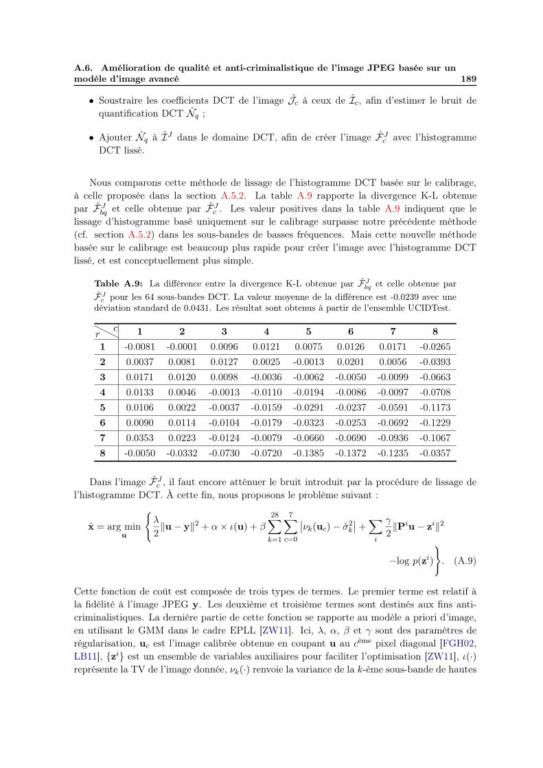
A.6. Amélioration de qualité et anti-criminalistique de l’image JPEG basée sur unmodèle d’image avancé 189
• Soustraire les coefficients DCT de l’image Jc à ceux de Ic, afin d’estimer le bruit dequantification DCT Nq ;
• Ajouter Nq à IJ dans le domaine DCT, afin de créer l’image FJc avec l’histogramme
DCT lissé.
Nous comparons cette méthode de lissage de l’histogramme DCT basée sur le calibrage,à celle proposée dans la section A.5.2. La table A.9 rapporte la divergence K-L obtenuepar FJ
bq et celle obtenue par FJc . Les valeur positives dans la table A.9 indiquent que le
lissage d’histogramme basé uniquement sur le calibrage surpasse notre précédente méthode(cf. section A.5.2) dans les sous-bandes de basses fréquences. Mais cette nouvelle méthodebasée sur le calibrage est beaucoup plus rapide pour créer l’image avec l’histogramme DCTlissé, et est conceptuellement plus simple.
Table A.9: La différence entre la divergence K-L obtenue par FJbq et celle obtenue par
FJc pour les 64 sous-bandes DCT. La valeur moyenne de la différence est -0.0239 avec une
déviation standard de 0.0431. Les résultat sont obtenus à partir de l’ensemble UCIDTest.
rc 1 2 3 4 5 6 7 8
1 -0.0081 -0.0001 0.0096 0.0121 0.0075 0.0126 0.0171 -0.0265
2 0.0037 0.0081 0.0127 0.0025 -0.0013 0.0201 0.0056 -0.0393
3 0.0171 0.0120 0.0098 -0.0036 -0.0062 -0.0050 -0.0099 -0.0663
4 0.0133 0.0046 -0.0013 -0.0110 -0.0194 -0.0086 -0.0097 -0.0708
5 0.0106 0.0022 -0.0037 -0.0159 -0.0291 -0.0237 -0.0591 -0.1173
6 0.0090 0.0114 -0.0104 -0.0179 -0.0323 -0.0253 -0.0692 -0.1229
7 0.0353 0.0223 -0.0124 -0.0079 -0.0660 -0.0690 -0.0936 -0.1067
8 -0.0050 -0.0332 -0.0730 -0.0720 -0.1385 -0.1372 -0.1235 -0.0357
Dans l’image FJc , il faut encore atténuer le bruit introduit par la procédure de lissage de
l’histogramme DCT. À cette fin, nous proposons le problème suivant :
x = arg minu
{
λ
2‖u− y‖2 + α× ι(u) + β
28∑
k=1
7∑
c=0
∣
∣νk(uc)− σ2k∣
∣+∑
i
γ
2‖Piu− zi‖2
−log p(zi)
}
. (A.9)
Cette fonction de coût est composée de trois types de termes. Le premier terme est relatif àla fidélité à l’image JPEG y. Les deuxième et troisième termes sont destinés aux fins anti-criminalistiques. La dernière partie de cette fonction se rapporte au modèle a priori d’image,en utilisant le GMM dans le cadre EPLL [ZW11]. Ici, λ, α, β et γ sont des paramètres derégularisation, uc est l’image calibrée obtenue en coupant u au cème pixel diagonal [FGH02,LB11], {zi} est un ensemble de variables auxiliaires pour faciliter l’optimisation [ZW11], ι(·)représente la TV de l’image donnée, νk(·) renvoie la variance de la k-ème sous-bande de hautes

190 Appendix A. Résumé en Français
fréquences (définie dans [LB11]) de l’image donnée, tandis que σ2k est la variance estimée del’image originale de la k-ème sous-bande de hautes fréquences de FJ
c .
FJ1 désigne notre image anti-criminalistique finale créée par la méthode proposée dans
cette section. La figure A.15 montre les courbes ROC obtenues par FJ0 contre des détecteurs
scalaires. En comparant la figure A.15 à la figure A.9-(f) et la figure A.13, on constate que laméthode proposée dans cette section ne surpasse pas les deux méthodes proposées précédem-ment. Cela apparaît également dans la table A.10. Une raison possible est que l’estimationdu bruit de quantification Nq est peut-être encore trop rudimentaire : cela introduit un bruitdans le domaine spatial, qui réduit non seulement l’indétectabilité criminalistique mais aussila qualité de l’image anti-criminalistique finale. La performance de la méthode proposée icipeut être améliorée par une estimation du bruit de quantification précise et l’intégration dedavantage de termes anti-criminalistiques dans l’équation (A.9). Par ailleurs, il est à noter quemême si la méthode décrite dans cette section n’est pas la meilleure parmi les trois méthodesanti-criminalistiques pour la compression JPEG, elle surpasse encore largement l’état de l’art(cf. la table A.10).
False positive rate
Truepositiverate
0 0.2 0.4 0.6 0.8 10
0.2
0.4
0.6
0.8
1
KF
KLuo
KQLuo
KV
KL
K1U
K2U
Random guess
Figure A.15: Les courbes ROC obtenues par FJ1 contre des détecteurs criminalistiques.
Les résultat sont obtenus à partir de l’ensemble UCIDTest.
A.7 Amélioration de la qualité et anti-criminalistique del’image filtrée par le filtre médian à l’aide d’une décon-volution variationnelle d’image
A.7.1 Introduction et motivation
Nous suivons la ligne de recherche décrite dans la section A.1.3.3, à savoir concevoir desméthodes anti-criminalistiques d’image en s’appuyant sur la restauration d’image. À cettefin, il faut un modèle pour décrire le processus de filtrage médian ainsi qu’un modèle a priori

A.7. Amélioration de la qualité et anti-criminalistique de l’image filtrée par le filtremédian à l’aide d’une déconvolution variationnelle d’image 191
Table A.10: De la deuxième colonne à la huitième colonne, sont listées les valeurs AUCpour différentes images contre des détecteurs scalaires ; la comparaison de la qualité d’image(avec I comme référence) est rapportée dans les deux dernières colonnes. Les résultats sontobtenus à partir de l’ensemble UCIDTest.
KF KLuo KQLuo KV KL K1
U K2U PSNR SSIM
J 0.9991 1.0000 0.9996 0.9976 0.9811 0.9860 0.8840 37.0999 0.9919
FJSqSb
0.3783 0.0806 0.6288 0.8337 0.5338 0.6309 0.4854 30.4591 0.9509
IJ 0.9997 0.9982 0.9528 0.7851 0.9698 0.9878 0.8779 37.8930 0.9927
FJc 0.9994 0.8147 0.5949 0.7383 0.9868 0.9868 0.8944 35.3209 0.9876
FJ1 0.5522 0.7291 0.3594 0.7394 0.5272 0.7750 0.5787 35.2568 0.9832
FJ0 0.6756 0.6046 0.5194 0.6210 0.4490 0.6772 0.5880 35.4814 0.9843
FJ 0.5398 0.6425 0.4598 0.6159 0.4344 0.5894 0.5317 35.9855 0.9866
d’image approprié afin de construire un problème d’optimisation basé sur le MAP pour leproblème inverse du filtrage médian.
De fait, le processus de filtrage médian pourrait être décrit comme une procédure deconvolution linéaire spatialement hétérogène. Pour une fenêtre locale, le noyau de convolutionest une matrice de taille 3 × 3 dont un seul des 9 éléments prendrait la valeur 1, et les 8autres éléments seraient tous nuls. La forme du noyau est alors complètement dépendante desstatistiques d’ordre des pixels encadrés par la fenêtre du filtre. Pourtant, cette information estdéfinitivement perdue pendant le processus de filtrage médian. Afin de simplifier ce modèle,la convolution avec un noyau spatialement homogène k est utilisée pour se rapprocher duprocessus de filtrage médian. L’analyse développée ici donnera le premier terme de l’équation(A.10) dans la section A.7.2.
Dans les méthodes criminalistiques proposées dans l’état de l’art [KF10, Cao+10, Yua11],la différence de valeurs de pixels d’image est souvent la caractéristique de base des détecteurs.En général, l’histogramme de différence de valeurs de pixels (à savoir la dérivée de l’image)a un pic plus haut dans l’image MF que celui de l’image originale, autour de la classe 0 (cf.les exemples dans la figure A.7). Pour régulariser la différence de valeurs de pixels, la loigaussienne généralisée (paramétrée par le paramètre d’échelle α et le paramètre de forme β)de moyenne nulle est utilisée pour la modéliser. L’analyse de ce paragraphe donnera le dernierterme de l’équation (A.10) dans la section A.7.2.
A.7.2 Déconvolution variationnelle d’image
D’une manière similaire à celle utilisée en anti-criminalistique de compression JPEG[Fan+13b], nous proposons un problème de déconvolution variationnelle d’image afin de créerune image MF anti-criminalistique, basé sur l’analyse développée dans la section A.7.1, et

192 Appendix A. Résumé en Français
dans une certaine mesure inspiré par [KF09, KTF11] :
arg minu
λ
2
(
‖Ku− y‖22 + ω ‖u− y‖22)
+J∑
j=1
∥
∥
∥
∥
Fju
αj
∥
∥
∥
∥
βj
βj
, (A.10)
Dans cette équation, y contient les valeurs des pixels de l’image MF sous forme vectorisée, cetteimage MF ayant été produite à partir de l’image originale x. La variable u est utilisée pourreprésenter génériquement une image. Ku désigne la multiplication matricielle correspondantà une convolution d’image avec le noyau k. J filtre(s) de dérivée d’image sont utilisés afinde calculer différents types de dérivées d’image. Fju est la multiplication matricielle servantà calculer la j-ème (j = 1, 2, · · · , J) dérivée d’image, en utilisant le j-ème filtre linéaire avecle noyau f j . αj et βj sont les deux paramètres de la loi gaussienne généralisée de moyennenulle utilisée pour modéliser la j-ème dérivée de l’image. λ et ω sont deux paramètres derégularisation pour équilibrer l’énergie des différents termes.
Il y a trois termes dans l’équation (A.10). Comme discuté ci-dessus, le processus de filtragemédian est simplifié, et approché par une convolution d’image avec un noyau spatialementhomogène – ce qui constitue le premier terme de l’équation (A.10). Le deuxième terme estconçu pour que l’image MF anti-criminalistique produite soit dans une certaine mesure prochede l’image MF. Le troisième terme est l’a priori d’image, qui sert à régulariser la dérivée del’image en utilisant la loi gaussienne généralisée de moyenne nulle. Dans la pratique, on utiliseles filtres suivants (J = 4) de dérivées d’image: f1 = [1,−1], f2 = [1,−1]T , f3 = [1, 0,−1], etf4 = [1, 0,−1]T . D’autres filtres pourraient être ajoutés dans l’équation (A.10), au prix d’unecomplexité de calcul plus élevée, mais pour un impact mineur sur les résultats finaux.
Pour le terme d’a priori d’image, il faut connaître les valeurs des deux paramètres α et β dela loi gaussienne généralisée de moyenne nulle. En fait, ces deux paramètres sont directementreliés à la variance σ2 et au kurtosis κ de la loi :
σ2 =α2Γ(3/β)
Γ(1/β), κ =
Γ(5/β)Γ(1/β)
Γ(3/β)2, (A.11)
où Γ(·) est la fonction gamma. Donc, si la variance et le kurtosis sont connus, les deuxparamètres α et β peuvent être estimés en utilisant une méthode numérique [BS99]. Parconséquent, il faut estimer la variance σ2 et la kurtosis κ de l’image originale à partir del’image MF. À cette fin, une régression linéaire est employée pour leur estimation, en utilisantl’image MF donnée et ses versions encore plusieurs fois filtrées par le filtre médian. Pour lej-ème type de filtre de dérivée d’image, la variance σ2(Fjx) et le kurtosis κ(Fjx) de l’imageoriginale sont estimés par :
σ2(Fjx) = cσ2
1 +∑M
m=1 cσ2
m+1 × σ2(
FjMF (m)(x))
,
κ(Fjx) = cκ1 +∑M
m=1 cκm+1 × κ
(
FjMF (m)(x))
,(A.12)
où σ2(·) et κ(·) sont respectivement la variance et le kurtosis de l’echantillon, et MF (m)(·)représente m applications successives du filtrage médian. cσ
2
m et cκm sont les coefficients de la

A.7. Amélioration de la qualité et anti-criminalistique de l’image filtrée par le filtremédian à l’aide d’une déconvolution variationnelle d’image 193
régression linéaire : ils peuvent être obtenus depuis un ensemble d’images par une procédured’apprentissage. Dans la pratique, fixer M à 5 donne de bons résultats.
L’optimisation directe de la fonction de coût dans l’équation (A.10) n’est pas triviale. Enpratique, elle peut être résolue en utilisant la méthode “ Half Quadratic Splitting ” [KF09]et la méthode de Bregman [GO09, KTF11]. Après l’introduction d’un ensemble de variablesauxiliaires {wj}Jj=1, le problème d’optimisation dans l’équation (A.10) peut être ré-écrit sousla forme suivante :
minu,{wj}
λ
2
(
‖Ku− y‖22 + ω ‖u− y‖22)
+
J∑
j=1
(γ
2
∥
∥Fju− αjwj∥
∥
2
2+∥
∥wj∥
∥
βj
βj
)
. (A.13)
où γ est un paramètre de régularisation. Ensuite, l’itération de Bregman est appliquée àl’équation (A.13). La méthode de Bregman résout le problème à la (k+1)-ème (k = 0, 1, 2, · · · )itération par les formules de l’équation (A.14), où {bj}Jj=1 sont les variables de Bregman, et
(bj)(0) = 0.
(
u(k+1), {(
wj)(k+1)}
)
= arg minu,{wj}
(
λ
2
(
‖Ku− y‖22 + ω ‖u− y‖22)
+J∑
j=1
(
γ
2
∥
∥
∥Fju+
(
bj)(k) − αjw
j∥
∥
∥
2
2+∥
∥wj∥
∥
βj
βj
)
)
,
(bj)(k+1) = (bj)(k) +(
Fju(k+1) − αj(wj)(k+1)
)
.
(A.14)
A.7.3 Amélioration de qualité de l’image MF
En paramétrant de manière appropriée, nous pouvons créer une image de meilleure qualité àpartir de l’image MF, en résolvant le problème d’optimisation dans l’équation (A.14). Pourestimer k dans l’équation (A.10), 6 types de noyaux ont été étudiés expérimentalement surl’ensemble MFTE100 : le noyau moyenne, le noyau gaussien, le noyau inspiré par [Yua11], et,pour chaque image, les trois noyaux estimés en utilisant les trois noyaux précédents commeestimation initiale pour la méthode [KTF11]. Les résultats expérimentaux montrent qu’unbon choix pour k est le noyau estimé par [KTF11] en utilisant le noyau moyenne commeestimation initiale. Pour l’amélioration de qualité de l’image MF, le paramétrage suivant estutilisé : ω = 0.4, λ = 1000 et γ = 1200. Ces paramètres sont obtenus depuis l’ensembleMFTE100.
La table A.11 compare la qualité d’image de l’image bruitée par le bruit sel et poivre, cellepuis filtrée par le filtre médian, puis à celle traitée par la méthode proposée. L’efficacité de ladéconvolution variationnelle d’image décrite dans la section A.7.2 est bien validée : la qualitéde l’image MF est améliorée en utilisant les métriques d’évaluation PSNR et SSIM. Ce fait

194 Appendix A. Résumé en Français
est aussi reflété par les valeurs PSNR/SSIM pour l’image Mp listées dans la table A.12, encomparaison avec l’image MF M.
Table A.11: Les valeurs moyennes du PSNR et du SSIM de l’image bruitée par le bruit selet poivre, celle puis filtrée par le filtre médian, et enfin celle traitée par la méthode proposée,respectivement. La densité de bruit varie de 1% à 7%. Les résultats sont obtenus à partirde l’ensemble MFTE.
Bruitée Filtrée Améliorée
1%PSNR 25.1365 37.1336 38.0723
SSIM 0.8308 0.9827 0.9892
2%PSNR 22.1257 36.9719 37.8236
SSIM 0.7185 0.9822 0.9885
3%PSNR 20.3642 36.7957 37.5155
SSIM 0.6388 0.9818 0.9876
4%PSNR 19.1161 36.6114 37.2058
SSIM 0.5793 0.9813 0.9867
5%PSNR 18.1466 36.4031 36.7914
oSSIM 0.5327 0.9807 0.9850
6%PSNR 17.3540 36.1758 36.2933
SSIM 0.4948 0.9801 0.9828
7%PSNR 16.6851 35.8924 35.7542
SSIM 0.4632 0.9793 0.9803
Table A.12: Du deuxième au troisième rang, sont listées les valeurs moyennes dePSNR/SSIM; les valeurs AUC pour différentes images contre des détecteurs scalaires sontrapportées dans les quatre rangs suivants ; les divergences K-L pour différents histogrammesde différence de valeurs de pixels sont listées dans les deux derniers rangs. Les résultats sontobtenus à partir de l’ensemble UCIDTest.
M Mp FMW FM
D FM
Qualité d’imagePSNR 37.2847 38.2953 33.6033 33.4272 37.5184
SSIM 0.9831 0.9896 0.9552 0.9714 0.9901
Performanceanti-criminalistique
KK 0.9722 0.7839 0.4592 0.5347 0.5595
KK 0.9824 0.8375 0.6586 0.4635 0.5061
KC 0.9938 0.8213 0.6668 0.7479 0.6490
KY 0.9984 0.7922 0.3336 0.6518 0.5886
divergence K-L
f1 0.1632 0.0990 0.1148 0.0547 0.0484
f2 0.1611 0.0949 0.1338 0.0563 0.0449
f3 0.0775 0.0525 0.0619 0.0383 0.0272
f4 0.0753 0.0495 0.0689 0.0389 0.0238

A.7. Amélioration de la qualité et anti-criminalistique de l’image filtrée par le filtremédian à l’aide d’une déconvolution variationnelle d’image 195
False positive rate
Truepositiverate
0 0.2 0.4 0.6 0.8 10
0.2
0.4
0.6
0.8
1
KK
KK
KC
KY
Random guess
(a)MFalse positive rate
Truepositiverate
0 0.2 0.4 0.6 0.8 10
0.2
0.4
0.6
0.8
1
KK
KK
KC
KY
Random guess
(b) FMW
False positive rate
Truepositiverate
0 0.2 0.4 0.6 0.8 10
0.2
0.4
0.6
0.8
1
KK
KK
KC
KY
Random guess
(c) FMD
False positive rate
Truepositiverate
0 0.2 0.4 0.6 0.8 10
0.2
0.4
0.6
0.8
1
KK
KK
KC
KY
Random guess
(d) FM
Figure A.16: Courbes ROC obtenues pour : l’image MF M, l’image produite par Wu et
al. FMW [WSL13], Dang-Nguyen et al. FM
D [DN+13], et la méthode proposée FM , contre
les quatre détecteurs scalaires KK [KF10], KK [KF10], KC [Cao+10], et KY [Yua11]. Lesrésultats sont obtenus à partir de l’ensemble MFTE.
A.7.4 Anti-criminalistique de filtrage médian
En résolvant le problème d’optimisation de l’équation (A.10) sur l’image MF, il est possiblede créer une image MF anti-criminalistique dotée d’une bonne immunité à la détection anti-criminalistique, mais sa qualité visuelle laissera à désirer. Afin d’obtenir une image MF anti-criminalistique présentant une bonne immunité sans beaucoup de diminution de la qualitéd’image, cette section propose une stratégie de perturbation légère de la valeur des pixels del’image MF, avant qu’elle soit utilisée dans l’équation (A.10).

196 Appendix A. Résumé en Français
Replacement rate
AUC
0 0.1 0.2 0.3 0.4 0.5 0.6 0.8 10.5
0.6
0.7
0.8
0.9
1
M
FM
W
FM
D
FM
(a) KS686SPAM [PBF10]
Replacement rate
AUC
0 0.1 0.2 0.3 0.4 0.5 0.6 0.8 10.5
0.6
0.7
0.8
0.9
1
M
FM
W
FM
D
FM
(b) KS44MFF [Yua11]
Replacement rate
AUC
0 0.1 0.2 0.3 0.4 0.5 0.6 0.8 10.5
0.6
0.7
0.8
0.9
1
M
FM
W
FM
D
FM
(c) KS56GLF [CNH13]
Replacement rate
AUC
0 0.1 0.2 0.3 0.4 0.5 0.6 0.8 10.5
0.6
0.7
0.8
0.9
1
M
FM
W
FM
D
FM
(d) KS10AR [Kan+13]
Replacement rate
AUC
0 0.1 0.2 0.3 0.4 0.5 0.6 0.8 10.5
0.6
0.7
0.8
0.9
1
M
FM
W
FM
D
FM
(e) KS220LTP [Zha+14]
Figure A.17: La valeur AUC en fonction du taux de remplacement d’image pour différentstypes d’images, lorsqu’elles sont testées en utilisant les détecteurs à base de SVM. Lesrésultats sont obtenus à partir de MFTR pour l’entraînement et à partir de MFTE pour lestests.
Les sorties de KK [KF10], KC [Cao+10] et KY [Yua11] sont toutes implicitement ou ex-plicitement reliées à une différence de valeurs de pixels, elles réagissent d’autant plus fortementdans les régions texturées de l’image. Le but ici est de réduire la fréquence d’occurrence de

A.8. Conclusions et perspectives 197
la différence 0 par une modification légère de l’image MF. Si trois pixels adjacents vérifientyi+1 = yi+2 = yi+3, la modification de yi+2 à yi+2±1 changera deux différences de valeurs depixel de 0 à ±1. De façon similaire, si deux pixels adjacents ont la même valeur, le pixel qui a lavariance locale plus élevée que l’autre est modifié. De cette manière, la fréquence d’occurrencede la différence 0 est efficacement réduite, avec un impact très limité sur la qualité de l’image.
De même qu’à la section A.7.3, pour k nous utilisons à nouveau le noyau estimé par[KTF11], avec le noyau moyenne comme estimation initiale. Afin de créer l’image MF anti-criminalistique en résolvant le problème d’optimisation de l’équation (A.13), le paramétragesuivant est utilisé : ω = 0.1, λ = 1500 et γ = 500. Ces paramètres sont obtenus depuisl’ensemble MFTE100.
Pour des raisons de concision, FM représente l’image MF anti-criminalistique créée àpartir de l’image MF par la méthode proposée. La table A.12 rapporte la qualité d’image (lesvaleurs de PSNR et de SSIM sont calculées en utilisant l’image originale comme référence) et laperformance anti-criminalistique. Les courbes ROC obtenues pour différents types d’images etpour les détecteurs KK [KF10], KC [Cao+10] ou KY [Yua11] sont tracées dans la figure A.16.Les images MF anti-criminalistiques FM créées par la méthode proposée induisent, pour lesdétecteurs criminalistiques, des courbes ROC qui sont au plus proche d’une décision aléatoire.Ce fait est également reflété par des valeurs AUC proches de 0.5 dans la table A.12 pour FM .De plus, la méthode proposée produit une meilleure qualité d’image que les autres imagesMF anti-criminalistiques de l’état de l’art [WSL13, DN+13]. Enfin, la table A.12 rapporte ladivergence K-L obtenue par FM et celles obtenues par les images anti-criminalistiques de l’étatde l’art. Les valeurs de la divergence K-L obtenues par FM sont plus petites, indiquant unemeilleure performance de la méthode proposée afin de restaurer l’histogramme de différencede valeurs de pixels que l’état de l’art. Les courbes AUC dans la figure A.17 montrent quenotre image anti-criminalistique a une meilleure indétectabilité criminalistique globale contreles détecteurs à base de SVM que l’état de l’art, sauf contre KS10
AR [Kan+13].
A.8 Conclusions et perspectives
A.8.1 Résumé des contributions
Dans cette thèse, nous avons présenté nos travaux de recherche sur l’anti-criminalistiqued’image sur la compression JPEG et le filtrage médian. Au cours de notre étude de l’anti-criminalistique d’image concernant le codage ou le traitement d’images, on constate des simil-itudes entre l’anti-criminalistique d’image et la restauration d’images. Toutes les deux visentà récupérer au mieux les informations perdues lors de la dégradation de l’image. Cependant,en plus de la qualité d’image, l’anti-criminalistique d’image a un autre objectif indispensable,i.e. : une bonne indétectabilité contre les détecteurs criminalistiques. À cette fin, nous intro-duisons des concepts/méthodes avancés de la restauration d’image pour concevoir de nouvellesméthodes anti-criminalistiques, en intégrant certains termes/stratégies anti-criminalistiques.Les résultats expérimentaux montrent que les méthodes proposées surpassent les méthodes
198 Appendix A. Résumé en Français
de l’état de l’art pour créer des images anti-criminalistiques avec une meilleure indétectabilitécriminalistique contre les détecteurs existants, ainsi qu’une meilleure qualité d’image. Bienque la restauration d’image elle-même ne soit pas notre sujet principal de recherche dans cettethèse, nous proposons également deux méthodes d’amélioration de la qualité d’image pour lacompression JPEG et le filtrage médian, respectivement. Elles servent d’étape préliminairedans les méthodes anti-criminalistiques proposées, mais sont également avérés avoir de bonnesperformances en termes de gain de PSNR/SSIM par rapport à l’image JPEG ou l’image MF.
Les contributions de cette thèse sont résumées comme suit.
Proposer une nouvelle ligne de recherche pour concevoir des méthodes anti-criminalistiques d’image via la restauration d’image : Après l’examen de la littéra-ture, nous trouvons courant d’utiliser le traitement d’image simple pour cacher les traceslaissées par une opération d’image ciblée aux fins d’anti-criminalistique. Par exemple, lefiltrage médian est utilisé pour l’anti-criminalistique JPEG afin d’éliminer les artefacts deblocage. L’injection de bruit est utilisée pour cacher les traces de filtrage médian. Ces méth-odes peuvent être efficaces pour attaquer détecteurs criminalistiques ciblés, mais peuvent parcontre être détectées par plusieurs détecteurs avancés. En outre, l’image anti-criminalistiquerésultante souffre d’une faible qualité visuelle, ce qui peut susciter spontanément le doutesur son authenticité. Dans cette thèse, nous proposons une nouvelle ligne de recherche ens’appuyant sur les concepts/méthodes avancés de la restauration d’image afin de concevoirdes méthodes d’anti-criminalistique d’image. Étant donnée une image dégradée par uneopération irréversible de traitement d’image, par exemple, la compression JPEG ou le fil-trage médian, l’objectif de l’anti-criminalistique d’image est de cacher les traces de traitementd’image tout en conservant une bonne qualité d’image. En se fondant sur les similitudes entrel’anti-criminalistique d’image et la restauration d’image, les cadres de travail et les termes del’optimisation introduits en restauration d’image aident à supprimer en partie les traces, touten gardant une bonne qualité d’image (même meilleur parfois) par rapport à l’image dégradéedonnée. La bonne performance anti-criminalistique est obtenue en ajoutant des termes anti-criminalistiques au cadre de l’optimisation ou en utilisant des stratégies anti-criminalistiquessupplémentaires. Nous suivons cette ligne de recherche tout au long de cette thèse pour l’anti-criminalistique de compression JPEG ainsi que l’anti-criminalistique de filtrage médian. Sasupériorité sur les méthodes anti-criminalistiques de l’état de l’art est bien prouvée par desrésultats expérimentaux, avec une meilleure indétectabilité criminalistique et une meilleurequalité de l’image traitée. À notre connaissance, nous sommes les premiers à utiliser systéma-tiquement la restauration aux fins d’anti-criminalistique. Nous espérons également que cettenouvelle ligne de recherche serait utile pour plusieurs problèmes d’anti-criminalistique d’imagerelatifs à d’autres traitements, par exemple le rééchantillonnage, l’amélioration du contraste,etc.
L’anti-criminalistique JPEG en utilisant le déblocage basé sur la TV : Nous avonsproposé une méthode anti-criminalistique de compression JPEG en utilisant la méthode dedéblocage basé sur la TV. Cela est mis en œuvre par l’optimisation d’un problème de min-imisation contraint basé sur la TV avec un terme de TV et un terme de mesure du déblocagepar la TV. Pendant ce temps, la qualité d’image traitée est contrôlée par une projection QCS

A.8. Conclusions et perspectives 199
modifiée. En outre, un détecteur puissant à base de calibrage est trompé par la minimisa-tion d’une fonction de coût proche de la fonction de calculant la caractéristique basée sur lecalibrage. Cette méthode parvient à bien éliminer les artefacts de blocage dans le domainespatial. En outre, les artefacts de quantification dans le domaine DCT sont aussi largementatténués, dans la mesure où l’image anti-criminalistique créée est capable de passer commen’ayant jamais été compressée face à des détecteurs scrutant les artefacts de quantification.
L’anti-criminalistique améliorée de compression JPEG avec une lissage perceptueld’histogramme DCT : En effet, la méthode de déblocage JPEG basée sur la TV précédem-ment proposée est capable de réaliser une bonne indétectabilité criminalistique contre tousles détecteurs criminalistiques actuels de compression JPEG existants, y compris ceux quiexaminant les artefacts de quantification. Cependant, l’histogramme DCT n’est pas toujoursbien lissé, en particulier dans les sous-bandes de moyennes fréquences. Cette faiblesse n’enest pas une face aux détecteurs criminalistiques actuels de compression JPEG, mais peut êtredétectée par des algorithmes criminalistiques potentiellement plus avancés. Afin de remédier àce problème, nous avons proposé une méthode anti-criminalistique améliorée en quatre étapesavec un lissage perceptuel de l’histogramme DCT. À l’aide des informations DCT estimées enpartie après le déblocage JPEG basé sur la TV, une méthode de tramage adaptatif local estproposée en combinant la loi de Laplace et la loi uniforme. Les coefficients DCT sont modifiéspar la résolution d’un problème d’affectation simplifié qui minimise la perte de qualité SSIM.On effectue un dernier déblocage léger basé sur la TV et le décalibrage pour améliorer encorel’indétectabilité criminalistique avec une perte de qualité d’image très mineure.
L’amélioration de qualité et l’anti-criminalistique de l’image JPEG basées sur unmodèle d’image avancé : Nous avons proposé une autre méthode anti-criminalistique JPEGbasé sur un modèle a priori d’image sophistiqué, qui est décrite par les étapes suivantes :
• L’amélioration de qualité d’image JPEG en utilisant un modèle a priori d’image so-
phistiqué : L’efficacité de l’utilisation de la TV dans l’anti-criminalistique JPEG nousmotive à utiliser les modèles a priori d’image plus sophistiqués, avec l’espoir d’améliorerles performances d’anti-criminalistique JPEG. À cette fin, nous utilisons le cadre EPLLavec le GMM comme a priori pour les patches d’image. Le bruit de compression dansle domaine spatial est modélisé en utilisant la loi gaussienne multivariée de moyennenulle, dont 64 types de matrices de covariance sont apprises pour chaque facteur dequalité JPEG. Par conséquent, un procédé d’amélioration de qualité d’image JPEG aété proposé en minimisant la fonction de coût en tenant compte des deux termes ci-dessus. L’image JPEG de qualité améliorée peut être obtenue en résolvant un problèmed’optimisation à l’aide d’une étape d’estimation approximative du MAP. Cette méthodenous permet d’obtenir un bon gain de qualité d’image pour l’image JPEG, en particulierpour la compression JPEG très forte.
• Le lissage non paramétrique d’histogramme DCT basé sur le calibrage : En plus denotre méthode de lissage perceptuel d’histogramme DCT précédemment proposé, nousproposons un autre lissage d’histogramme DCT basé cette fois sur le calibrage, sansutiliser aucun modèle statistique. Basé sur les statistiques d’image et l’efficacité de

200 Appendix A. Résumé en Français
l’astuce du calibrage, le bruit de quantification dans le domaine DCT peut être estiméen découpant légèrement l’image JPEG de qualité améliorée et en recompressant l’imagecalibrée. L’histogramme DCT est lissé en ajoutant le bruit de quantification DCT estiméà partir de l’image JPEG de qualité améliorée. Cette nouvelle méthode de lissage non-paramétrique d’histogramme DCT ne permet pas d’obtenir une meilleure performanceglobale, mais a de meilleures performances dans les sous-bande DCT de basses fréquencesque la méthode de lissage perceptuel précédemment proposée. En outre, la méthodebasée sur le calibrage a un coût de calcul beaucoup plus faible que la perceptuelle.
• L’indétectabilité criminalistique est considérée au travers de la minimisation d’une fonc-tion de coût avec un terme d’image de fidélité, une terme d’a priori d’image à based’EPLL, et plusieurs termes anti-criminalistiques inspirés des algorithmes criminalis-tiques existants.
Pour récapituler, la méthode proposée pour l’amélioration de la qualité JPEG est illustrée pardes expériences sur 4 images classiques de test et sur l’ensemble UCIDTest pour améliorerla qualité de l’image JPEG. En effet, la méthode anti-criminalistique proposée doit êtreaméliorée, mais surpasse encore les méthodes de l’état de l’art proposées par Stamm et al.
[Sta+10a, Sta+10b, SL11] en termes d’indétectabilité criminalistique ainsi que de qualité del’image traitée.
L’amélioration de qualité et l’anti-criminalistique de l’image MF via une décon-volution variationnelle d’image : Nous avons proposé une déconvolution variationnelled’image pour à la fois l’amélioration de qualité de l’image MF et l’anti-criminalistique de fil-trage médian. Un noyau de convolution spatialement homogène est utilisé pour approcher leprocessus de filtrage médian. En ce qui concerne l’a priori d’image, la loi gaussienne général-isée de moyenne nulle est utilisée pour modéliser la différence de valeurs de pixels dont lesstatistiques changement considérablement après filtrage médian. Basé sur l’analyse ci-dessus,la fonction de coût de minimisation proposée est composée d’un terme de convolution, d’unterme de fidélité d’image par rapport à l’image MF, et d’un terme d’a priori. L’image MF dequalité améliorée peut être obtenue en résolvant ce problème de minimisation, avec une qualitéd’image meilleure que l’image MF. Avec un autre paramétrage et une perturbation de valeur depixel supplémentaire, l’image anti-criminalistique est également générée depuis l’image MF.La méthode proposée est capable d’atteindre une indétectabilité criminalistique contre lesdétecteurs criminalistiques actuels de filtrage médian et une qualité d’image meilleures parrapport aux méthodes anti-criminalistiques de filtrage médian de l’état de l’art.
En résumé, la caractéristique/nouveauté principale de cette thèse est d’introduiredes concepts/méthodes avancés de la restauration d’image pour concevoir des méthodesd’anti-criminalistique d’image. Plus précisément, nous avons conçu des méthodes anti-criminalistiques pour la compression JPEG et le filtrage médian, misant sur les élémentssuivants de la restauration d’image : la TV, le cadre de EPLL avec le GMM comme mod-èle d’a priori pour les patches d’image, et le cadre de déconvolution d’images fondé sur leMAP. Pour un problème anti-criminalistique d’image donné, certains termes/stratégies anti-criminalistiques sont intégrés pour tromper les détecteurs existants. Pour la compression

A.8. Conclusions et perspectives 201
JPEG, un terme de mesure de blocage JPEG basé sur la TV est utilisé pour le déblocageJPEG. En outre, deux méthodes de lissage d’histogramme DCT sont proposées pour sup-primer les artefacts de quantification dans le domaine DCT : une procédure de lissage per-ceptuel de l’histogramme DCT, et une procédure non paramétrique de lissage de l’histogrammeDCT basé sur le décalibrage. Certains termes anti-criminalistiques inspirés des algorithmescriminalistiques existants sont également intégrés dans le cadre de l’optimisation à base deMAP, pour tromper les détecteurs criminalistiques. Quant au filtrage médian, le modèle d’apriori d’image est choisi spécifiquement afin de régulariser les différences de valeurs de pixelsd’image, qui sont explicitement ou implicitement utilisées dans les algorithmes criminalistiquesexistants. En outre, une procédure de perturbation de valeur de pixel est également proposéeafin d’améliorer encore l’indétectabilité criminalistique, avec perte très mineure de qualitéd’image.
A.8.2 Perspectives
À court terme, les perspectives de cette thèse comprennent l’amélioration de la performance del’anti-criminalistique d’image, et la poursuite de la ligne de recherche proposée pour concevoirdes méthodes anti-criminalistiques concernant d’autres traitements.
L’amélioration de l’anti-criminalistique d’image JPEG pour générer l’image anti-criminalistique avec une qualité plus haute que l’image JPEG : Dans les sections A.4-A.5, la TV est employée depuis la restauration d’image aux fins d’anti-criminalistique JPEG.La TV peut être considéré comme un a priori d’image simple mais efficace. La section A.6présente la suite logique sur l’anti-criminalistique de compression JPEG, où un a priori plussophistiqué que la TV est utilisé. Cependant, la nouvelle méthode anti-criminalistique JPEGne surpasse pas celles basées sur la TV. L’analyse et les possibles raisons en sont fournies à lafin de la section A.6.3. Un problème anti-criminalistique difficile mais très intéressant pour lacompression JPEG est de savoir si on peut créer l’image anti-criminalistique avec une qualitéencore plus élevé que l’image JPEG, ne serait-ce que pour montrer la relativité de ces mesures.Une direction de recherche possible pourrait être la combinaison de l’amélioration de la qualitéde l’image JPEG, le déblocage basé sur la TV, et le lissage perceptuel d’histogramme DCT.En fait, un objectif similaire a déjà été réalisé dans la section A.7.4 pour le filtrage médian :l’image anti-criminalistique MF a une qualité encore plus élevée que l’image MF dans le testsur l’ensemble MFTE.
Le développement d’autres méthodes anti-criminalistiques en misant sur la restau-ration d’image : Dans cette thèse, nous avons choisi de travailler sur la compression JPEGet le filtrage médian pour l’anti-criminalistique d’image. En traitement d’image, il existe beau-coup d’autres opérations dont le problème d’anti-criminalistique peut également être formulécomme un problème inverse mal posé. Par exemple, l’anti-criminalistique du rééchantillonnagepeut partager certaines similitudes avec la super-résolution [PPK03]. L’anti-criminalistiqued’amélioration du contraste peut être liée à l’estimation de la transformation de la lumi-nosité des pixels [ZL14]. Idéalement, une bonne performance anti-criminalistique ne peut êtreatteinte que si des concepts/méthodes de la restauration d’image sont bien combinés avec
202 Appendix A. Résumé en Français
certains termes/stratégies anti-criminalistiques.
À long terme, l’un des buts ultimes de la criminalistique d’image et de l’anti-criminalistiqueest de développer des méthodes universelles sans viser des méthodes (anti-)criminalistiquesspécifiques. Cela afin d’éviter au maximum un éternel “ jeu du chat et de la souris ” entrela criminalistique et l’anti-criminalistique. Bien que le travail de recherche de criminalistique(ou d’anti-criminalistique) d’image s’étale maintenant sur plus d’une décennie, il existe trèspeu de méthodes universelles. Actuellement, la seule méthode anti-criminalistique d’image estprobablement celle proposée par Barni et al. [BFT12]. Toutefois, elle fait aussi l’hypothèseque les détecteurs criminalistiques examinent seulement les statistiques du premier ordre.Nous sommes conscients que les méthodes anti-criminalistiques proposées appartiennent tousà la catégorie “ ciblées ” selon la classification d’anti-criminalistique d’image proposée parBöhme et Kirchner [BK13]. Cependant, nous croyons que les méthodes anti-criminalistiquesproposées ont le potentiel requis pour être généralisées en vue du développement d’une anti-criminalistique d’image universelle.
Vers une anti-criminalistique d’image universelle: Dans les sections A.6-A.7, lesproblèmes d’optimisation à base de MAP sont proposées pour calculer les images anti-criminalistiques de compression JPEG et de filtrage médian, respectivement. L’universalitédu cadre de restauration d’image variationnelle peut être vu à travers ces deux problèmes.En matière de codage/traitement d’images, l’objectif de l’anti-criminalistique est de créer uneimage anti-criminalistique qui soit aussi “ naturelle ” que possible. À cette fin, le problèmede la génération d’image “ naturelle ” peut être formulé comme un problème de restaurationd’image, pour obtenir une image qui semble n’avoir jamais été traitée. Afin de résoudre cetype de problèmes inverses, on peut utiliser des méthodes statistiques comme l’estimateurdu MAP. Dans ce cadre, un bon modèle d’a priori d’image est indispensable. Par ailleurs, leterme de vraisemblance, qui décrit le processus de dégradation de l’image causée par un certaintraitement d’image, devrait varier en fonction de différents problèmes anti-criminalistiques. “L’universalité ” ici est que le cadre anti-criminalistique est générique : il peut être utilisé pourcacher les traces laissées par diverses autres opérations de traitement d’image.
En outre, certains autres problèmes de recherche ouverts et étroitement liés à cette thèsesont répertoriés comme suit :
• Est-il possible de concevoir une attaque en une seule étape pour l’anti-criminalistiqued’image JPEG, compte tenu que plusieurs détecteurs criminalistiques travaillent dansdeux domaines différents ?
• Comment peut-on estimer le noyau de convolution spatialement hétérogène pour le fil-trage médian ?
• Est-il possible de créer une image anti-criminalistique, de sorte que dans son ensem-ble elle puisse paraître comme jamais traitée face aux détecteurs à base de méthodesd’apprentissage automatique ?
Ces questions soulignent également quelques directions futures de recherche intéressantes dans

A.8. Conclusions et perspectives 203
le vaste domaine de l’anti-criminalistique d’image. En outre, concernant le lien étroit entrel’image et la vidéo, les méthodes d’anti-criminalistique d’image proposées sur la compressionJPEG et le filtrage médian peuvent également certainement contribuer à l’anti-criminalistiquede vidéo.
Dans cette thèse, nous procédons à l’étude de l’anti-criminalistique d’image de compres-sion JPEG et de filtrage médian, en s’inspirant de la restauration d’image. Ces deux prob-lèmes spécifiques d’anti-criminalistique d’image constituent seulement une petite fraction del’anti-criminalistique d’image. Nous sommes également conscients que cette ligne de recherchenouvellement formée peut être appliquée uniquement aux problèmes d’anti-criminalistiqued’image, où le codage/traitement d’image est impliqué. Pour les autres problèmes d’anti-criminalistique d’image, par exemple, celui basé sur la physique ou la géométrie [Far09a], cetteligne de recherche peut être inadéquate. Par exemple, dans notre travail d’anti-criminalistiqued’image basé sur l’estimation environnementale de lumière [Fan+12], c’est une tout autre lignede recherche qui est suivie.
En conclusion, pour les problèmes d’anti-criminalistique d’image impliquant descodages/traitements d’image, nous croyons que les statistiques d’images naturelles sont es-sentielles dans la création d’une image anti-criminalistique avec une bonne indétectabilitécriminalistique ainsi qu’une haute qualité d’image. À cette fin, certains concepts/méthodesavancés de la restauration d’image sont introduits et combinés avec des termes/stratégies anti-criminalistiques pour la compression JPEG et le filtrage médian. Les travaux de rechercheprésentés dans cette thèse ne représentent qu’une petite partie du potentiel énorme desstatistiques d’images naturelles appliquées à l’anti-criminalistique d’image, la criminalis-tique d’image et la restauration d’image. Böhme et Kirchner [BK13] soulignent égalementl’importance du modèle statistique d’image naturelle dans la bataille entre la criminalistiqueet l’anti-criminalistique. Par conséquent, en dépit de beaucoup de points sujets à améliora-tion, notre travail peut servir de bon point de départ pour de futures recherches sur un largeéventail de problèmes criminalistiques et anti-criminalistiques.


Bibliography
[ADF05] F. Alter, S. Durand, and J. Froment. “Adapted total variation for artifact freedecompression of JPEG images”. Journal of Mathematical Imaging and Vision
23, 2 (2005), pp. 199–211 (Cited on pages xxii, 6, 26, 35, 48, 53, 55–59, 62, 70,97, 166, 178).
[Aig] Huaqi: the secret to self-innovation in the market. http://tech.sina.com.cn/it/2005-12-21/1432798682.shtml (in Chinese) (Cited on pages 2, 161).
[BFP11] P. Bas, T. Filler, and T. Pevný. “Break our steganographic system — the insand outs of organizing BOSS”. In: Proceedings of the International Conference on
Information Hiding (IH). Santa Barbara, California, USA, 2011, pp. 59–70 (Citedon pages 23, 24, 49, 50).
[BFT12] M. Barni, M. Fontani, and B. Tondi. “A universal technique to hide traces ofhistogram-based image manipulations”. In: Proceedings of the ACM Workshop on
Multimedia and Security (MMSec). Coventry, UK, 2012, pp. 97–104 (Cited onpages 77, 157, 202).
[BK13] R. Böhme and M. Kirchner. “Counter-forensics: attacking image forensics”. In:Digital Image Forensics. Ed. by H. T. Sencar and N. Memon. New York: Springer,2013, pp. 327–366 (Cited on pages 3, 12–14, 19, 20, 49, 53, 125, 157, 158, 163,167–169, 202, 203).
[Bov87] A. C. Bovik. “Streaking in median filtered images”. IEEE Transactions on Acous-
tics, Speech and Signal Processing 35, 4 (1987), pp. 493–503 (Cited on pages 40,41, 176).
[BP12a] T. Bianchi and A. Piva. “Detection of nonaligned double JPEG compression basedon integer periodicity maps”. IEEE Transactions on Information Forensics and
Security 7, 2 (2012), pp. 842–848 (Cited on pages 24, 89, 90, 92, 93, 96).
[BP12b] T. Bianchi and A. Piva. “Image forgery localization via block-grained analysis ofJPEG artifacts”. IEEE Transactions on Information Forensics and Security 7, 3(2012), pp. 1003–1017 (Cited on pages 4, 24, 89, 90, 93–95, 164).
[BS99] R. W. Buccigrossi and E. P. Simonceli. “Image compression via joint statisticalcharacterization in the wavelet domain”. IEEE Transactions on Image Processing
8, 12 (1999), pp. 1688–1701 (Cited on pages 128, 192).
[BV04] S. Boyd and L. Vandenberghe. Convex optimization. New York: Cambridge Uni-versity Press, 2004 (Cited on page 55).
[BXM03] S. Boyd, L. Xiao, and A. Mutapcic. Subgradient methods. Tech. rep. EE392o.Stanford University, 2003 (Cited on pages 25, 26, 173).
[Cao+10] G. Cao, Y. Zhao, R. Ni, L. Yu, and H. Tian. “Forensic detection of medianfiltering in digital images”. In: Proceedings of the IEEE International Conference
on Multimedia and Expo (ICME). Singapore, 2010, pp. 89–94 (Cited on pages 42,44, 45, 127, 137, 138, 140–143, 146, 147, 150, 173, 177, 191, 195–197).
205

206 Bibliography
[Cha09] R. Chartrand. “Fast algorithms for nonconvex compressive sensing: MRI recon-struction from very few data”. In: Proceedings of IEEE International Symposium
on Biomedical Imaging: From Nano to Macro (ISBI). Boston, Massachusetts,USA, 2009, pp. 262–265 (Cited on pages 29, 131).
[Che+12] C. Chen, J. Ni, R. Huang, and J. Huang. “Blind median filtering detection usingstatistics in difference domain”. In: Proceedings of the International Conference
on Information Hiding (IH). Berkeley, California, USA, 2012, pp. 1–15 (Cited onpages 43, 45, 127, 177).
[CL11] C.-C. Chang and C.-J. Lin. “LIBSVM: a Library for support vector machines”.ACM Transactions on Intelligent Systems and Technology 2, (3 2011). Softwareavailable at http://www.csie.ntu.edu.tw/~cjlin/libsvm, 27:1–27:27 (Citedon pages 18, 19, 90, 144).
[CN11] C. Chen and J. Ni. “Median filtering detection using edge based prediction ma-trix”. In: Proceedings of the International Workshop on Digital Forensics and Wa-
termarking (IWDW). Atlantic City, New Jersey, USA, 2011, pp. 361–375 (Citedon pages 43, 127).
[CNH13] C. Chen, J. Ni, and J. Huang. “Blind detection of median filtering in digitalimages: a difference domain based approach”. IEEE Transactions on Image Pro-
cessing 22, 12 (2013), pp. 4699–4710 (Cited on pages 43, 45, 127, 144, 145, 148,151, 177, 196).
[Con11] V. Conotter. “Active and passive multimedia forensics”. PhD thesis. Universityof Trento, 2011 (Cited on pages 2, 161, 162).
[CS08] C. Chen and Y. Q. Shi. “JPEG image steganalysis utilizing both intrablock andinterblock correlations”. In: Proceedings of the IEEE International Symposium on
Circuits and Systems (ISCAS). Seattle, Washington, USA, 2008, pp. 3029–3032(Cited on pages 38, 39, 64, 86, 87, 175, 187).
[DN+13] D. T. Dang-Nguyen, I. D. Gebru, V. Conotter, G. Boato, and F. G. B. De Natale.“Counter-forensics of median filtering”. In: Proceedings of the IEEE International
Workshop on Multimedia Signal Processing (MMSP). Pula, Sardinia, Italy, 2013,pp. 260–265 (Cited on pages xxiii, 24, 40, 44–46, 138, 141–144, 146, 147, 149, 150,176, 177, 195, 197).
[Fan+12] W. Fan, K. Wang, F. Cayre, and Z. Xiong. “3-D lighting-based image forgerydetection using shape-from-shading”. In: Proceedings of the European Signal Pro-
cessing Conference (EUSIPCO). Bucharest, Romania: IEEE, 2012, pp. 1777–1781(Cited on pages 158, 203).
[Fan+13a] W. Fan, K. Wang, F. Cayre, and Z. Xiong. “A variational approach to JPEG anti-forensics”. In: Proceedings of the IEEE International Conference on Acoustics,
Speech, and Signal Processing (ICASSP). Vancouver, Canada, 2013, pp. 3058–3062 (Cited on pages 7, 47, 113, 149).

Bibliography 207
[Fan+13b] W. Fan, K. Wang, F. Cayre, and Z. Xiong. “JPEG anti-forensics using non-parametric DCT quantization noise estimation and natural image statistics”. In:Proceedings of ACM International Workshop on Information Hiding and Multi-
media Security (IHMMSec). Montpellier, France, 2013, pp. 117–122 (Cited onpages 7, 105, 113, 116, 118, 191).
[Fan+14] W. Fan, K. Wang, F. Cayre, and Z. Xiong. “JPEG anti-forensics with improvedtradeoff between forensic undetectability and image quality”. IEEE Transactions
on Information Forensics and Security 9, 8 (2014), pp. 1211–1226 (Cited onpages 7, 66, 113).
[Fan+15] W. Fan, K. Wang, F. Cayre, and Z. Xiong. “Median filtered image quality en-hancement and anti-forensics via variational deconvolution”. IEEE Transactions
on Information Forensics and Security (2015) (Cited on page 124).
[Far06] H. Farid. Digital image ballistics from JPEG quantization. Tech. rep. TR2006-583.Department of Computer Science, Dartmouth College, 2006 (Cited on pages 10,12, 168).
[Far09a] H. Farid. “A survey of image forgery detection”. IEEE Signal Processing Magazine
2, 26 (2009), pp. 16–25 (Cited on pages 2, 10, 14, 34, 158, 162, 165, 167, 169, 203).
[Far09b] H. Farid. “Exposing digital forgeries from JPEG ghosts”. IEEE Transactions on
Information Forensics and Security 1, 4 (2009), pp. 154–160 (Cited on page 37).
[FB12] M. Fontani and M. Barni. “Hiding traces of median filtering in digital im-ages”. In: Proceedings of the European Signal Processing Conference (EUSIPCO).Bucharest, Romania: IEEE, 2012, pp. 1239–1243 (Cited on pages 24, 40, 44, 45,138, 141, 176).
[FD00] Z. Fan and R. L. De Queiroz. “Maximum likelihood estimation of JPEG quanti-zation table in the identification of bitmap compression history”. In: Proceedings
of the IEEE International Conference on Image Processing (ICIP). Vancouver,Canada, 2000, pp. 948–951 (Cited on page 49).
[FD03] Z. Fan and R. L. De Queiroz. “Identification of bitmap compression history: JPEGdetection and quantizer estimation”. IEEE Transactions on Image Processing 12,2 (2003), pp. 230–235 (Cited on pages 6, 23, 24, 36, 37, 39, 49–51, 53, 57, 60, 61,64, 67, 69, 80, 116–118, 149, 150, 166, 174, 175).
[FGH02] J. Fridrich, M. Goljan, and D. Hogea. “Steganalysis of JPEG images: breakingthe F5 algorithm”. In: Proceedings of the International Workshop on Information
Hiding (IH). Noordwijkerhout, the Netherlands, 2002, pp. 310–323 (Cited onpages 7, 38, 106, 112, 116, 166, 189).
[Fou] Fourandsix Technologies, Inc. http://www.fourandsix.com/about-us/ (Citedon pages 2, 161).
[Fri93] G. L. Friedman. “The trustworthy digital camera: restoring credibility to thephotographic image”. IEEE Transactions on Consumer Electronics 39, 4 (1993),pp. 905–910 (Cited on pages 2, 161).

208 Bibliography
[GO09] T. Goldstein and S. Osher. “The split Bregman method for ℓ1-regularized prob-lems”. SIAM Journal on Imaging Sciences 2, 2 (2009), pp. 323–343 (Cited onpages 28, 29, 131, 173, 193).
[GY95] D. Geman and C. Yang. “Nonlinear image recovery with half-quadratic regular-ization”. IEEE Transactions on Image Processing 4, 7 (1995), pp. 932–946 (Citedon pages 27, 173).
[HF13] V. Holub and J. Fridrich. “Digital image steganography using universal distor-tion”. In: Proceedings of the ACM International Workshop on Information Hiding
and Multimedia Security (IHMMSec). Montpellier, France, 2013, pp. 59–68 (Citedon page 19).
[Iee] IEEE Xplore digital library. http://ieeexplore.ieee.org (Cited on pages 3,162).
[Ijg] The independent JPEG group. http://www.ijg.org (Cited on page 32).
[Kan+12] X. Kang, M. C. Stamm, A. Peng, and K. J. R. Liu. “Robust median filteringforensics based on the autoregressive model of median filtered residual”. In: Pro-
ceedings of the Asia-Pacific Signal Information Processing Association Annual
Summit and Conference. Hollywood, California, USA, 2012, pp. 1–9 (Cited onpages 43, 45, 127, 177).
[Kan+13] X. Kang, M. C. Stamm, A. Peng, and K. J. R. Liu. “Robust median filtering foren-sics using an autoregressive model”. IEEE Transactions on Information Forensics
and Security 8, 9 (2013), pp. 1456–1468 (Cited on pages 43, 45, 127, 144, 145,148, 151, 177, 196, 197).
[KB07] M. Kirchner and R. Böhme. “Tamper hiding: defeating image forensics”. In: Pro-
ceedings of the International Conference on Information Hiding (IH). Saint Malo,France, 2007, pp. 326–341 (Cited on pages 3, 163).
[KF09] D. Krishnan and R. Fergus. “Fast image deconvolution using hyper-Laplacianpriors”. In: Proceedings of the Neural Information Processing Systems (NIPS).Vancouver, Canada, 2009, pp. 1033–1041 (Cited on pages 7, 27, 125, 129–131,166, 192, 193).
[KF10] M. Kirchner and J. Fridrich. “On detection of median filtering in digital images”.In: Proceedings of the SPIE: Media Forensics and Security II. San Jose, California,USA, 2010, 754110:1–754110:12 (Cited on pages 41, 42, 44, 45, 127, 137, 138, 140,142, 143, 146, 147, 150, 173, 177, 191, 195–197).
[KL51] S. Kullback and R. A. Leibler. “On information and sufficiency”. Annals of Math-
ematical Statistics 22, 1 (1951), pp. 49–86 (Cited on pages 15, 22, 172).
[KR08] M. Kirchner and R. Röhme. “Hiding traces of resampling in digital images”. IEEE
Transactions on Information Forensics and Security 3, 4 (2008), pp. 582–592(Cited on pages 4, 5, 121, 125, 146, 163, 165).
Bibliography 209
[KTF11] D. Krishnan, T. Tay, and R. Fergus. “Blind deconvolution using a normalizedsparsity measure”. In: Proceedings of the IEEE Conference on Computer Vi-
sion and Pattern Recognition (CVPR). Colorado Springs, Colorado, USA, 2011,pp. 233–240 (Cited on pages 7, 29, 125, 131, 132, 166, 192, 193, 197).
[Kuh55] H. W. Kuhn. “The Hungarian method for the assignment problem”. Naval Re-
search Logistics Quarterly 2, 1-2 (1955), pp. 83–97 (Cited on pages 26, 77, 81,173).
[LB11] S. Lai and R. Böhme. “Countering counter-forensics: the case of JPEG compres-sion”. In: Proceedings of the International Conference on Information Hiding (IH).Prague, Czech Republic, 2011, pp. 285–298 (Cited on pages 37–39, 53, 56, 57, 60,61, 80, 86, 112, 116–118, 175, 179, 189, 190).
[Lev+09] A. Levin, Y. Weiss, F. Durand, and W. T. Freeman. “Understanding and evalu-ating blind deconvolution algorithms”. In: Proceedings of the IEEE Conference on
Computer Vision and Pattern Recognition (CVPR). Miami, Florida, USA, 2009,pp. 1964–1971 (Cited on page 125).
[LG00] E. Y. Lam and J. W. Goodman. “A mathematical analysis of the DCT coefficientdistributions for images”. IEEE Transactions on Image Processing 9, 10 (2000),pp. 1661–1666 (Cited on pages 36, 71).
[LHQ10] W. Luo, J. Huang, and G. Qiu. “JPEG error analysis and its applications to digitalimage forensics”. IEEE Transactions on Information Forensics and Security 5, 3(2010), pp. 480–491 (Cited on pages 36, 39, 53, 60, 64, 67, 69, 175).
[LLH12] H. Li, W. Luo, and J. Huang. “Countering anti-JPEG compression forensics”. In:Proceedings of the IEEE International Conference on Image Processing (ICIP).Orlando, Florida, USA, 2012, pp. 241–244 (Cited on pages 38, 39, 64, 86, 87, 175,186, 187).
[LY04] A. W.-C. Liew and H. Yan. “Blocking artifacts suppression in block-coded imagesusing overcomplete wavelet representation”. IEEE Transactions on Circuits and
Systems for Video Technology 14, 4 (2004), pp. 450–461 (Cited on pages 35, 48,53).
[Mar] Mary Meeker’s state of the Internet. http://moonlighthk.com/mary-meekers-state-internet (Cited on pages 1, 160).
[MB04] F. Melgani and L. Bruzzone. “Classification of hyperspectral remote sensing im-ages with support vector machines”. IEEE Transactions on Geoscience and Re-
mote Sensing 42, 8 (2004), pp. 1778–1790 (Cited on page 19).
[PBF10] T. Pevný, P. Bas, and J. Fridrich. “Steganalysis by subtractive pixel adjacencymatrix”. IEEE Transactions on Information Forensics and Security 5, 2 (2010),pp. 215–224 (Cited on pages 18, 19, 38, 39, 42–45, 64, 86, 87, 127, 144, 145, 148,151, 175, 177, 186, 187, 196).
[PF05] A.C. Popescu and H. Farid. “Exposing digital forgeries by detecting traces ofresampling”. IEEE Transactions on Signal Processing 53, 2 (2005), pp. 758–767(Cited on pages 146, 147).

210 Bibliography
[PF08] T. Pevný and J. Fridrich. “Detection of double-compression in JPEG images forapplications in steganography”. IEEE Transactions on Information Forensics and
Security 3, 2 (2008), pp. 247–258 (Cited on pages 89–91).
[Piv13] A. Piva. “An overview on image forensics”. ISRN Signal Processing (2013), 22:1–22:22 (Cited on pages 11, 12, 14, 167).
[PK12] A. Peng and X. Kang. “Robust median filtering detection based on filtered resid-ual”. In: Proceedings of the International Workshop on Digital Forensics and Wa-
termarking (IWDW). Shanghai, China, 2012, pp. 344–357 (Cited on pages 43,127).
[PM93] W. B. Pennebaker and J. L. Mitchell. JPEG still image data compression stan-
dard. New York: Van Nostrand Reinhold, 1993 (Cited on page 32).
[PPK03] S. C. Park, M. K. Park, and M. G. Kang. “Super-resolution image reconstruction:a technical overview”. IEEE Signal Processing Magazine 20, 3 (2003), pp. 21–36(Cited on pages 157, 201).
[PR99] J. R. Price and M. Rabbani. “Biased reconstruction for JPEG decoding”. IEEE
Signal Processing Letters 6, 12 (1999), pp. 297–299 (Cited on pages 71, 76, 111).
[PV92] I. Pitas and A. N. Venetsanopoulos. “Order statistics in digital image processing”.Proceedings of IEEE 80, 12 (1992), pp. 1893–1921 (Cited on page 40).
[ROF92] L. I. Rudin, S. Osher, and E. Fatemi. “Nonlinear total variation based noiseremoval algorithms”. Physica D: Nonlinear Phenomena 60, 1-4 (1992), pp. 259–268 (Cited on pages 37, 48, 178).
[RS05] M. A. Robertson and R. L. Stevenson. “DCT quantization noise in compressedimages”. IEEE Transactions on Circuits and Systems for Video Technology 15, 1(2005), pp. 27–38 (Cited on pages 6, 7, 34–36, 57, 72, 73, 97, 106–109, 166, 174,183).
[RTD11] J. A. Redi, W. Taktak, and J.-L. Dugelay. “Digital image forensics: a booklet forbeginners”. Multimedia Tools and Applications 51, 1 (2011), pp. 133–162 (Citedon pages 10, 11, 14, 167).
[Sal03] P. Sallee. Matlab JPEG toolbox. Available at http://dde.binghamton.edu/
download/feature_extractors/. 2003 (Cited on pages 33, 55).
[SC07] D. Sun and W.-K. Cham. “Postprocessing of low bit-rate block DCT coded imagesbased on a fields of experts prior”. IEEE Transactions on Image Processing 16,11 (2007), pp. 2743–2751 (Cited on pages 35, 57, 97, 106–110, 188).
[SL11] M. C. Stamm and K. J. R. Liu. “Anti-forensics of digital image compression”.IEEE Transactions on Information Forensics and Security 6, 3 (2011), pp. 1050–1065 (Cited on pages xxii, 4–6, 36–40, 46, 48, 49, 52, 53, 58, 60, 63, 64, 67, 71,76, 81–90, 92, 96, 106, 110–113, 116, 118, 119, 121, 125, 146, 149, 155, 163, 165,175, 177, 180, 181, 185, 200).

Bibliography 211
[SS04] G. Schaefer and M. Stich. “UCID - an uncompressed colour image database”.In: Proceedings of the SPIE: Storage and Retrieval Methods and Applications for
Multimedia. San Jose, California, USA, 2004, pp. 472–480 (Cited on pages 22–24,50, 51, 56, 60, 71, 72, 89, 172, 183, 184).
[SS11] P. Sutthiwan and Y. Q. Shi. “Anti-forensics of double JPEG compression detec-tion”. In: Proceedings of the International Workshop on Digital Forensics and Wa-
termarking (IWDW). Atlantic City, New Jersey, USA, 2011, pp. 411–424 (Citedon pages xxii, 22, 38–40, 52, 53, 58, 60, 62, 89–91, 93, 118, 121, 172, 175, 180,181).
[Sta+10a] M. Stamm, S. Tjoa, W. S. Lin, and K. J. R. Liu. “Anti-forensics of JPEG compres-sion”. In: Proceedings of the IEEE International Conference on Acoustics, Speech,
and Signal Processing (ICASSP). Dallas, Texas, USA, 2010, pp. 1694–1697 (Citedon pages xxii, 22, 36–40, 48, 49, 52, 53, 58, 60, 63, 64, 67, 71, 74, 76, 81–92, 96,106, 110–113, 116, 118, 119, 121, 125, 149, 155, 172, 175, 180, 181, 185, 200).
[Sta+10b] M. Stamm, S. Tjoa, W. S. Lin, and K. J. R. Liu. “Undetectable image tamperingthrough JPEG compression anti-forensics”. In: Proceedings of the IEEE Interna-
tional Conference on Image Processing (ICIP). Hongkong, China, 2010, pp. 2109–2112 (Cited on pages xxii, 22, 37–40, 46, 48, 52, 53, 58, 60, 63, 64, 67, 85–92, 96,116, 118, 119, 121, 125, 149, 155, 172, 175, 177, 180, 181, 200).
[SWL13] M. C. Stamm, M. Wu, and K. J. R. Liu. “Information forensics: an overview ofthe first decade”. IEEE Access 1, (2013), pp. 167–200 (Cited on pages 12–14,167).
[TT10] X. Tan and B. Triggs. “Enhanced local texture feature sets for face recognitionunder difficult lighting conditions”. IEEE Transactions on Image Processing 19,6 (2010), pp. 1635–1650 (Cited on page 43).
[UW08] C. Ullerich and A. Westfeld. “Weaknesses of MB2”. In: Proceedings of the Inter-
national Workshop on Digital Watermarking (IWDW). Guangzhou, China, 2008,pp. 127–142 (Cited on page 51).
[Val+11] G. Valenzise, V. Nobile, M. Tagliasacchi, and S. Tubaro. “Countering JPEG anti-forensics”. In: Proceedings of the IEEE International Conference on Image Pro-
cessing (ICIP). Brussels, Belguim, 2011, pp. 1949–1952 (Cited on pages 37, 39,53, 60, 86, 116, 118, 175).
[Vap98] V. N. Vapnik. The nature of statistical learning theory. Second. Springer, 1998(Cited on page 19).
[VPPG11] D. Vázquez-Padín and F. Pérez-González. “Prefilter design for forensic resamplingestimation”. In: Proceedings of the IEEE International Workshop on Information
Forensics and Security (WIFS). Iguacu Falls, Brazil, 2011, pp. 1–6 (Cited onpage 24).
[VPPG12] D. Vázquez-Padín and F. Pérez-González. “ML estimation of the resampling fac-tor”. In: Proceedings of the IEEE International Workshop on Information Foren-
sics and Security (WIFS). Tenerife, Spain, 2012, pp. 205–210 (Cited on page 24).

212 Bibliography
[VTT11] G. Valenzise, M. Tagliasacchi, and S. Tubaro. “The cost of JPEG compressionanti-forensics”. In: Proceedings of the IEEE International Conference on Acous-
tics, Speech, and Signal Processing (ICASSP). Prague, Czech Republic, 2011,pp. 1884–1887 (Cited on pages xxii, 22, 37, 39, 40, 52, 53, 58, 60, 62, 74, 81–83,86, 89–91, 111, 118, 121, 172, 175, 180, 181).
[VTT13] G. Valenzise, M. Tagliasacchi, and S. Tubaro. “Revealing the traces of JPEG com-pression anti-forensics”. IEEE Transactions on Information Forensics and Secu-
rity 8, 2 (2013), pp. 335–349 (Cited on pages 37–39, 53, 60, 86, 118, 175).
[W3t] http://w3techs.com/technologies/overview/image_format/all (Cited onpages 4, 164).
[Wan+04] Z. Wang, A. C. Bovik, H. R. Sheikh, and E. P. Simoncelli. “Image quality assess-ment: from error visibility to structural similarity”. IEEE Transactions on Image
Processing 13, 4 (2004), pp. 600–612 (Cited on pages 21, 22, 77, 133, 171).
[WB06] Z. Wang and A. C. Bovik. Modern image quality assessment. Morgan & Claypool,2006 (Cited on pages 21, 171).
[WN09] Z. Wei and K. N. Ngan. “Spatio-temporal just noticeable distortion profile for greyscale image/video in DCT domain”. IEEE Transactions on Circuits and Systems
for Video Technology 19, 3 (2009), pp. 337–346 (Cited on page 37).
[WSL13] Z.-H. Wu, M. C. Stamm, and K. J. R. Liu. “Anti-forensics of median filtering”.In: Proceedings of the IEEE International Conference on Acoustics, Speech, and
Signal Processing (ICASSP). Vancouver, Canada, 2013, pp. 3043–3047 (Cited onpages xxiii, 4, 6, 24, 25, 40, 44, 45, 128, 138, 141–144, 146, 147, 149, 150, 163,165, 176, 195, 197).
[YGK95] Y. Yang, N. Galatsanos, and A. Katsaggelos. “Projection-based spatially adap-tive reconstruction of block-transform compressed images”. IEEE Transactions
on Image Processing 4, 7 (1995), pp. 896–908 (Cited on pages 35, 57).
[Yua11] H.-D. Yuan. “Blind forensics of median filtering in digital images”. IEEE Trans-
actions on Information Forensics and Security 6, 4 (2011), pp. 1335–1345 (Citedon pages 42, 44, 45, 127, 132, 137, 138, 140–148, 150, 151, 173, 177, 191, 193,195–197).
[Zha+08] G. Zhai, W. Zhang, X. Yang, W. Lin, and Y. Xu. “Efficient image deblockingbased on postfiltering in shifted windows”. IEEE Transactions on Circuits and
Systems for Video Technology 18, 1 (2008), pp. 122–126 (Cited on pages 35, 48,53).
[Zha+10] B. Zhang, Y. Gao, S. Zhao, and J. Liu. “Local derivative pattern versus localbinary pattern: face recognition with high-order local pattern descriptor”. IEEE
Transactions on Image Processing 19, 2 (2010), pp. 533–544 (Cited on page 44).
[Zha+14] Y. Zhang, S. Li, S. Wang, and Y. Q. Shi. “Revealing the traces of median filteringusing high-order local ternary patterns”. IEEE Signal Processing Letters 21, 3(2014), pp. 275–280 (Cited on pages 43, 45, 127, 144, 145, 148, 151, 177, 196).

Bibliography 213
[ZL14] X. Zhang and S. Lyu. “Blind estimation of pixel brightness transform”. In: Pro-
ceedings of the IEEE International Conference on Image Processing (ICIP). Paris,France, 2014, pp. 4472–4476 (Cited on pages 157, 201).
[ZW11] D. Zoran and Y. Weiss. “From learning models of natural image patches to wholeimage restoration”. In: Proceedings of the International Conference on Computer
Vision (ICCV). Barcelona, Spain, 2011, pp. 479–486 (Cited on pages 7, 27, 29,36, 97, 106, 108, 109, 116, 117, 131, 166, 188, 189).


Author’s Publications
International Journals
• Wei Fan, Kai Wang, François Cayre, and Zhang Xiong, “JPEG anti-forensics with im-proved tradeoff between forensic undetectability and image quality”, IEEE Transactions
on Information Forensics and Security, vol. 9, no. 8, pp. 1211-1226, 2014.
• Wei Fan, Kai Wang, François Cayre, and Zhang Xiong, “Median filtered image qualityenhancement and anti-forensics via variational deconvolution”, IEEE Transactions on
Information Forensics and Security, vol. 10, no. 5, pp. 1076-1091, 2015.
International Conferences
• Wei Fan, Kai Wang, François Cayre, and Zhang Xiong, “3-D lighting-based imageforgery detection using shape-from-shading”, In: Proceedings of the European Signal
Processing Conference (EUSIPCO), Bucharest, Romania: IEEE, 2012, pp. 1777-1781.
• Wei Fan, Kai Wang, François Cayre, and Zhang Xiong, “A variational approach toJPEG anti-forensics”, In: Proceedings of the IEEE International Conference on Acous-
tics, Speech, and Signal Processing (ICASSP), Vancouver, Canada, 2013, pp. 3058-3062.
• Wei Fan, Kai Wang, François Cayre, and Zhang Xiong, “JPEG anti-forensics usingnon-parametric DCT quantization noise estimation and natural image statistics”, In:Proceedings of the ACM International Workshop on Information Hiding and Multimedia
Security (IHMMSec), Montpellier, France, 2013, pp. 117-122. (Best Paper Award)
• Meijuan Wang, Zhenyong Chen, Wei Fan, and Zhang Xiong, “Countering anti-forensicsto wavelet-based compression”, In: Proceedings of the IEEE International Conference on
Image Processing (ICIP), Paris, France, 2014, pp. 5382-5386.
Local Conference
• Wei Fan, Kai Wang, François Cayre, and Zhang Xiong, “Empêcher la détection crim-inalistique de filtrage médian en images numériques”, In: Proceedings of the Colloque
Gretsi - Communauté Francophone du Traitement du Signal et des Images, Lyon, France,2015. (in French)
215


Title: Towards Digital Image Anti-Forensics via Image Restoration
Abstract: Image forensics enjoys its increasing popularity as a powerful image au-thentication tool, working in a blind passive way without the aid of any a priori embeddedinformation compared to fragile image watermarking. On its opponent side, image anti-forensics attacks forensic algorithms for the future development of more trustworthy forensics.When image coding or processing is involved, we notice that image anti-forensics to someextent shares a similar goal with image restoration. Both of them aim to recover theinformation lost during the image degradation, yet image anti-forensics has one additionalindispensable forensic undetectability requirement. In this thesis, we form a new research linefor image anti-forensics, by leveraging on advanced concepts/methods from image restorationmeanwhile with integrations of anti-forensic strategies/terms. Under this context, thisthesis contributes on the following four aspects for JPEG compression and median filteringanti-forensics: (i) JPEG anti-forensics using Total Variation based deblocking, (ii) improvedTotal Variation based JPEG anti-forensics with assignment problem based perceptual DCThistogram smoothing, (iii) JPEG anti-forensics using JPEG image quality enhancementbased on a sophisticated image prior model and non-parametric DCT histogram smoothingbased on calibration, and (iv) median filtered image quality enhancement and anti-forensicsvia variational deconvolution. Experimental results demonstrate the effectiveness of theproposed anti-forensic methods with a better forensic undetectability against existing forensicdetectors as well as a higher visual quality of the processed image, by comparisons with thestate-of-the-art methods.
Keywords: Anti-forensics, digital image, image restoration, JPEG compression, me-dian filtering

Titre : Vers l’anti-criminalistique en images numériques via la restauration d’images
Résumé : La criminalistique en images numériques se développe comme un outilpuissant pour l’authentification d’image, en travaillant de manière passive et aveugle sansl’aide d’informations d’authentification pré-intégrées dans l’image (contrairement au tatouagefragile d’image). En parallèle, l’anti-criminalistique se propose d’attaquer les algorithmes decriminalistique afin de maintenir une saine émulation susceptible d’aider à leur amélioration.En images numériques, l’anti-criminalistique partage quelques similitudes avec la restaurationd’image : dans les deux cas, l’on souhaite approcher au mieux les informations perduespendant un processus de dégradation d’image. Cependant, l’anti-criminalistique se doit deremplir au mieux un objectif supplémentaire, i.e. : être non détectable par la criminalistiqueactuelle. Dans cette thèse, nous proposons une nouvelle piste de recherche pour la criminalis-tique en images numériques, en tirant profit des concepts/méthodes avancés de la restaurationd’image mais en intégrant des stratégies/termes spécifiquement anti-criminalistiques. Dansce contexte, cette thèse apporte des contributions sur quatre aspects concernant, en crimi-nalistique JPEG, (i) l’introduction du déblocage basé sur la variation totale pour contrer lesméthodes de criminalistique JPEG et (ii) l’amélioration apportée par l’adjonction d’un lissageperceptuel de l’histogramme DCT, (iii) l’utilisation d’un modèle d’image sophistiqué et d’unlissage non paramétrique de l’histogramme DCT visant l’amélioration de la qualité de l’imagefalsifiée; et, en criminalistique du filtrage médian, (iv) l’introduction d’une méthode fondéesur la déconvolution variationnelle. Les résultats expérimentaux démontrent l’efficacité desméthodes anti-criminalistiques proposées, avec notamment une meilleure indétectabilité faceaux détecteurs criminalistiques actuels ainsi qu’une meilleure qualité visuelle de l’imagefalsifiée par rapport aux méthodes anti-criminalistiques de l’état de l’art.
Mots clés : Anti-criminalistique, image numérique, restauration d’image, compres-sion JPEG, filtrage médian
GIPSA-lab, 11 rue des Mathématiques, Grenoble Campus BP 46,F-38402 Saint Martin d’Hères CEDEX, France