Towards an Algebraic Theory of Boolean Circuits

Yves Lafont∗

February 12, 2003

Abstract

Boolean circuits are used to represent programs on finite data. Reversible Boolean circuits andquantum Boolean circuits have been introduced to modelize some physical aspects of computation.Those notions are essential in complexity theory, but we claim that a deep mathematical theory isneeded to make progress in this area. For that purpose, the recent developments of knot theory is amajor source of inspiration.

Following the ideas of Burroni, we consider logical gates as generators for some algebraic structurewith two compositions, and we are interested in the relations satisfied by those generators. For thatpurpose, we introduce canonical forms and rewriting systems. Up to now, we have mainly studiedthe basic case and the linear case, but we hope that our methods can be used to get presentationsby generators and relations for the (reversible) classical case and for the (unitary) quantum case.

Keywords: boolean circuit; reversible gate; monoidal category; presentation by generators and relations;canonical form; rewriting; symmetric group; alternating group; linear group; orthogonal group.

1 Introduction

We use diagrams to represent certain kinds of maps. If p and q are natural numbers, φ : p → q standsfor a diagram with p inputs and q outputs. It is pictured as follows:

· · ·φ

q︸︷︷︸

︷︸︸︷p

· · ·

Typically, such a diagram represents:

• a map from {1, . . . , p} to {1, . . . , q} (basic case);

• a map from Xp to Xq, where X is a given set (classical case);

• a K-linear map from Kp to Kq, where K is a given field (linear case);

• a K-linear map from⊗pV to

⊗qV , where V is a given vector space over a field K, and⊗nV

stands for the n-ary tensor product V ⊗ · · · ⊗ V (quantum case).

The basic case corresponds to control flow diagrams and the classical case to data flow diagrams.

Diagrams may be composed in two different ways. For any φ : p → q and ψ : q → r, we have a diagramψ ◦ φ : p→ r, which corresponds to the usual composition of maps, and which is pictured as follows:

· · ·

· · ·

· · ·

φ

ψ

This vertical (or sequential) composition is associative, and we have an identity diagram idp : p → p foreach p, such that φ ◦ idp = φ = idq ◦ φ for any φ : p→ q. This idp is pictured as follows:

· · ·

∗Universite de la Mediterranee & Institut de Mathematiques de Luminy, UPR 9016 du CNRS, 163 avenue de Luminy,

case 930, 13288 Marseille Cedex 9, France. E-mail: lafont@iml.univ-mrs.fr

1

For any φ : p→ q and φ′ : p′ → q′, we have a diagram φ | φ′ : p+ p′ → q+ q′ which is pictured as follows:

· · ·

· · ·φ

· · ·φ′· · ·

If φ represents f and φ′ represents f ′, the interpretation g of φ | φ′ depends on the considered case:

• in the basic case, g is the disjoint union (or coproduct) f ⊎ f ′ defined by g(i) = f(i) for i = 1, . . . , pand g(p+ i) = q + f ′(i) for i = 1, . . . , p′;

• in the classical case, g is the cartesian product f × f ′ defined by g(x1, . . . , xp+p′ ) = (y1, . . . , yq+q′)where (y1, . . . , yq) = f(x1, . . . , xp) and (yq+1, . . . , yq+q′) = f ′(xp+1, . . . , xp+p′);

• in the linear case, g is the direct sum f ⊕ f ′ defined by g(u ⊕ u′) = f(u) ⊕ f ′(u′) for u ∈ Kp andu′ ∈ Kp′

. Note that g coincides with the cartesian product f × f ′;

• in the quantum case, g is the tensor product f⊗f ′ defined by g(u⊗u′) = f(u)⊗f ′(u′) for u ∈⊗p

V

and u′ ∈⊗p′

V .

This horizontal (or parallel) composition is associative, and the void diagram id0 : 0 → 0 is such thatφ | id0 = φ = id0 |φ for any φ : p→ q. Furthermore, we have idp | idp′ = idp+p′ , and the two compositionsare compatible in the following sense: for any φ : p→ q, ψ : q → r, φ′ : p′ → q′, and ψ′ : q′ → r′, we have(ψ ◦ φ) | (ψ′ ◦ φ′) = (ψ | ψ′) ◦ (φ | φ′). This diagram is pictured as follows:

· · ·

· · ·

· · ·

φ

ψ

· · ·φ′· · ·

· · ·ψ′

In particular, for any φ : p→ q and φ′ : p′ → q′, we get (φ | idq′) ◦ (idp | φ′) = φ | φ′ = (idq | φ

′) ◦ (φ | idp′).This corresponds to the following picture:

· · ·φ

· · ·φ′

· · ·

· · ·

φ φ′· · ·

· · · · · ·

· · ·

· · ·φ′

· · ·φ

· · ·

· · ·

= =

All this can be summarized as follows: the diagrams are the morphisms of a (strict) monoidal categorywhose objects are natural numbers (with addition). See [Mac71] for the notion of monoidal category.Moreover, this monoidal category is freely generated by a given list of atomic diagrams called cells. Inother words, all diagrams are built from identities and cells using vertical and horizontal composition,and an equality between two diagrams holds only if it follows from the above properties.

An elementary diagram is a diagram ξ of the form idi | α | idj where α is a cell:

· · ·α· · ·

· · · · · ·

It is easy to see that any diagram φ is a vertical composition of elementary diagrams ξ1 ◦ · · · ◦ ξn, but thisdecomposition is not unique. In fact, two decompositions define the same diagram if and only if they areequivalent modulo the following commutation rule:

· · · · · ·· · ·

· · ·α

· · · · · ·α′

· · ·

· · ·α

· · ·α′

· · ·

· · ·

· · ·

· · ·· · · =

In particular, all decompositions of φ have the same length. This common length is called the size of φ:it is the total number of cells in φ.

Diagrams may be interpreted in any monoidal category. We have already seen four examples:

• sets with disjoint union (basic case) or with cartesian product (classical case);

• vector spaces with direct sum (linear case) or with tensor product (quantum case).

We may also consider monoidal subcategories obtained by restricting the class of objects or the class ofmorphisms. For instance, we may limit our study to finite sets or to finite dimensional spaces, to bijective,surjective, or injective maps, and whenever it makes sense, to monotone, orthogonal, or unitary maps. Inthis paper, we give presentations by generators and relations for some of those monoidal categories.

2

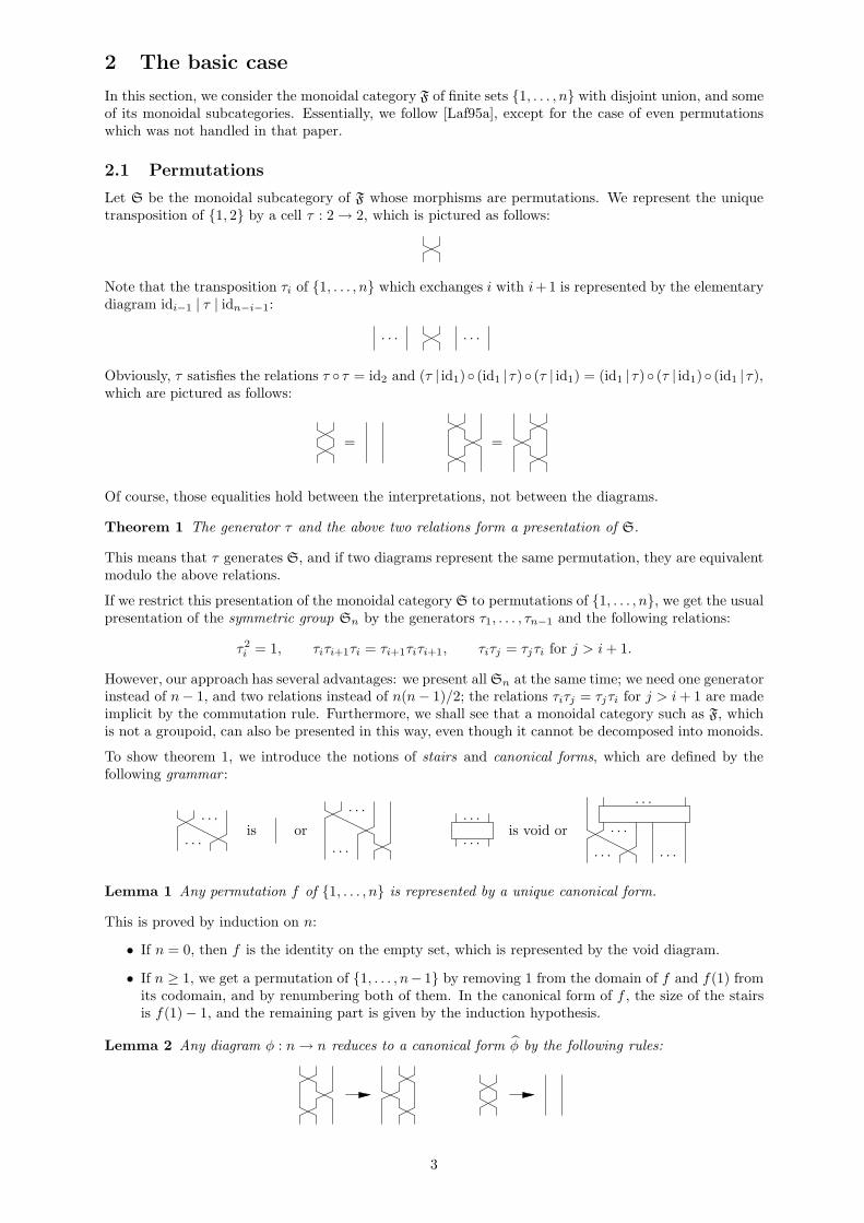
2 The basic case

In this section, we consider the monoidal category F of finite sets {1, . . . , n} with disjoint union, and someof its monoidal subcategories. Essentially, we follow [Laf95a], except for the case of even permutationswhich was not handled in that paper.

2.1 Permutations

Let S be the monoidal subcategory of F whose morphisms are permutations. We represent the uniquetransposition of {1, 2} by a cell τ : 2 → 2, which is pictured as follows:

Note that the transposition τi of {1, . . . , n} which exchanges i with i+1 is represented by the elementarydiagram idi−1 | τ | idn−i−1:

· · · · · ·

Obviously, τ satisfies the relations τ ◦ τ = id2 and (τ | id1)◦ (id1 | τ)◦ (τ | id1) = (id1 | τ)◦ (τ | id1)◦ (id1 | τ),which are pictured as follows:

= =

Of course, those equalities hold between the interpretations, not between the diagrams.

Theorem 1 The generator τ and the above two relations form a presentation of S.

This means that τ generates S, and if two diagrams represent the same permutation, they are equivalentmodulo the above relations.

If we restrict this presentation of the monoidal category S to permutations of {1, . . . , n}, we get the usualpresentation of the symmetric group Sn by the generators τ1, . . . , τn−1 and the following relations:

τ2i = 1, τiτi+1τi = τi+1τiτi+1, τiτj = τjτi for j > i+ 1.

However, our approach has several advantages: we present all Sn at the same time; we need one generatorinstead of n− 1, and two relations instead of n(n− 1)/2; the relations τiτj = τjτi for j > i+ 1 are madeimplicit by the commutation rule. Furthermore, we shall see that a monoidal category such as F, whichis not a groupoid, can also be presented in this way, even though it cannot be decomposed into monoids.

To show theorem 1, we introduce the notions of stairs and canonical forms, which are defined by thefollowing grammar :

· · ·

· · ·

· · ·

· · ·

oris· · ·

· · ·· · ·

· · ·· · ·

· · ·is void or

Lemma 1 Any permutation f of {1, . . . , n} is represented by a unique canonical form.

This is proved by induction on n:

• If n = 0, then f is the identity on the empty set, which is represented by the void diagram.

• If n ≥ 1, we get a permutation of {1, . . . , n− 1} by removing 1 from the domain of f and f(1) fromits codomain, and by renumbering both of them. In the canonical form of f , the size of the stairsis f(1) − 1, and the remaining part is given by the induction hypothesis.

Lemma 2 Any diagram φ : n→ n reduces to a canonical form φ by the following rules:

3

This is proved by double induction on n and the size m of φ:

• If m = 0, then φ = idn, which is a canonical form. This is easily checked by induction on n.

• If m ≥ 1, then φ = ξ ◦ ψ where ξ is an elementary diagram and ψ is a diagram of size m− 1 whichreduces to a canonical form ψ by induction hypothesis. Therefore, φ reduces to ξ ◦ ψ and there arefour possible cases: see figure 1. In the first case, we use the first rule and the induction hypothesisfor n− 1; in the second case, we use the second rule and we get a canonical form; in the third case,we get a canonical form; in the fourth case, we use the induction hypothesis for n− 1. Note thatin the first and in the last case, we also need the commutation rule, which is implicit.

Now we can prove theorem 1: τ generates S by lemma 1, and if two diagrams φ and ψ represent thesame permutation, then φ reduces to φ and ψ to ψ by lemma 2. Since all those diagrams represent thesame permutation, we have φ = ψ by lemma 1, so that φ and ψ are equivalent modulo the relations.

In fact, our rules form a terminating rewrite system: see appendix A. Since they do not increase the sizeof diagrams, a canonical form is always a diagram of minimal size for the map it represents.

2.2 Monotone maps

Let M be the monoidal subcategory of F whose morphisms are monotone maps. We introduce twogenerators µ : 2 → 1 and η : 0 → 1, which are interpreted in the obvious way and pictured as follows:

Obviously, µ and η satisfy the relations µ◦ (µ | id1) = µ◦ (id1 |µ), µ◦ (η | id1) = id1, and µ◦ (id1 |η) = id1,which are pictured as follows:

= = =

Theorem 2 The generators µ, η and the above three relations form a presentation of M.

To show this, we introduce the following notion of canonical form:

· · ·

· · ·

· · ·

· · ·

· · ·

· · ·

is void or or

Lemma 3 Any monotone map f : {1, . . . , p} → {1, . . . , q} is represented by a unique canonical form.

This is proved by induction on n = p+ q:

• If n = 0, then f is the identity on the empty set, which is represented by the void diagram.

• If p ≥ 1 and f(1) = 1, we get a monotone map by removing 1 from the domain of f , and byrenumbering it. The canonical form is of the second type, and the remaining part is given by theinduction hypothesis.

• Otherwise, q ≥ 1 and 1 is not in the image of f : we get a monotone map by removing 1 from thecodomain of f , and by renumbering it. The canonical form is of the third type, and the remainingpart is given by the induction hypothesis.

Lemma 4 Any diagram φ : p→ q reduces to a canonical form φ by the following rules:

This is proved by double induction on n = p+ q and the size m of φ:

• If m = 0, then φ = idp, which reduces to a canonical form. This is proved by induction on p, usingthe first rule:

· · ·

· · ·

· · ·· · ·

4

• If m ≥ 1, then φ = ξ ◦ ψ where ξ is an elementary diagram and ψ is a diagram of size m− 1 whichreduces to a canonical form ψ by induction hypothesis. Therefore, φ reduces to ξ ◦ ψ and thereare seven possible cases: see figure 2. In the first case, we use the second rule and the inductionhypothesis for n− 1; in the second case, we use the third rule and we get a canonical form; in thefifth case, we get a canonical form; in the other four cases, we use the induction hypothesis for n−1.

Theorem 2 follows from lemma 3 and lemma 4.

Note that identity diagrams are not in canonical form, so that the above rewrite system is not terminating.This can be fixed by adopting the alternative canonical form of figure 3, which consists in decomposingany monotone map f : {1, . . . , p} → {1, . . . , q} into a monotone surjection g : {1, . . . , p} → {1, . . . , n}followed by a monotone injection h : {1, . . . , n} → {1, . . . , q}, and the terminating rewrite system offigure 4. By the way, we get:

• a presentation of the monoidal subcategory Msurj of M whose morphisms are monotone surjectionsby one generator µ and the relation µ ◦ (µ | id1) = µ ◦ (id1 | µ);

• a presentation of the monoidal subcategory Minj of M whose morphisms are monotone injectionsby one generator η and no relation.

2.3 Maps

Any map f : {1, . . . , p} → {1, . . . , q} can be decomposed into a permutation g : {1, . . . , p} → {1, . . . , p}followed by a monotone map h : {1, . . . , p} → {1, . . . , q}. This decomposition is not unique, but it showsthat the monoidal category F is generated by τ , µ, and η:

These generators satisfy the relations of figure 5, which consist of: the two relations for S; the first tworelations for M; three extra relations τ ◦ (µ | id1) = (id1 | µ) ◦ (τ | id1) ◦ (id1 | τ), τ ◦ (η | id1) = id1 | η, andµ ◦ τ = µ. Note that the third relation for M is derivable: see figure 7.

Theorem 3 The generators τ , µ, η and the seven relations of figure 5 form a presentation of F.

To show this, we introduce the following notion of canonical form:

· · ·· · ·

· · ·

· · ·

· · ·· · ·

· · ·oris

It is easy to see that any map is represented by a unique canonical form. Now we introduce the rules offigure 6, which are derivable from the above relations: see figure 7. To show that any identity diagramreduces to a canonical form, we need a slightly more general result:

Lemma 5 The diagram η | · · · | η | idp reduces to a canonical form.

This is proved by induction on p, using the two reversible rules:

· · ·

· · ·

· · ·

· · ·

· · ·

· · ·

· · ·· · ·

· · ·

· · ·· · ·

· · ·

Theorem 3 follows from the fact that any diagram reduces to a canonical form by the rules of figure 6.In fact, it is also possible to show that our presentation is minimal: see [Mas97a].

Again, the rewrite system of figure 6 is not terminating, but we can adopt the alternative canonicalform of figure 8, which consists in decomposing any map f : {1, . . . , p} → {1, . . . , q} into a surjectiong : {1, . . . , p} → {1, . . . , n} followed by a monotone injection h : {1, . . . , n} → {1, . . . , q}, and theterminating rewrite system of figure 9: see appendix A. By the way, we get:

• a presentation of the monoidal subcategory Fsurj of F whose morphisms are surjections by τ , µ,and the five relations of figure 5 which do not involve η;

• a presentation of the monoidal subcategory Finj of F whose morphisms are injections by τ , η, andthe three relations of figure 5 which do not involve µ.

5

· · ·

· · ·

· · ·

· · ·

· · · · · ·

· · ·

· · ·

· · · · · ·

· · ·

· · ·· · ·

· · ·

· · ·

· · · · · · · · ·

· · ·

Figure 1: The four cases of lemma 2

· · ·

· · ·· · ·

· · ·· · · · · ·

· · ·

· · · · · ·

· · ·

· · · · · ·

· · ·· · ·

· · · · · ·

· · ·

· · ·

Figure 2: The seven cases of lemma 4

· · ·

· · ·· · ·

· · ·

· · ·

is

· · ·

· · ·

· · ·

· · ·

· · ·

· · ·

is void or or

· · ·

· · ·

· · ·

· · ·

· · ·

· · ·is void or or

Figure 3: Alternative canonical form for M

Figure 4: Alternative rules for M

==

===

= =

Figure 5: Relations for F

6

Figure 6: Rules for F

= = = = = = = =

= == = =

Figure 7: Deriving rules for F

· · ·

· · ·

· · ·

· · ·

· · ·

· · ·is void or or

· · ·

· · ·

· · ·

· · ·

· · ·

· · ·

· · ·

· · ·· · ·

· · ·is void or or

· · ·

· · ·· · ·

· · ·

· · ·

is

Figure 8: Alternative canonical form for F

Figure 9: Alternative rules for F

7

2.4 Even permutations

Finally, we consider the monoidal subcategory A of S whose morphisms are even permutations. An evenpermutation is a product of an even number of transpositions. The simplest one is a cyclic permutationof order 3. So we introduce a generator ω : 3 → 3, which is pictured and defined as follows:

=

Obviously, ω satisfies the following relations:

= = =

Theorem 4 The generator ω and the above three relations form a presentation of A.

Note that the second relation can be replaced by the following one:

=

If we restrict this presentation of the monoidal category A to even permutations of {1, . . . , n}, we get apresentation of the alternating group An by the generators ω1, . . . , ωn−2 and the following relations:

ω3i = 1, (ωiωi+1)

2 = 1, ωiωi+2ωi = ωi+1ωiωi+2, ωiωj = ωjωi for j > i+ 2.

To show theorem 4, we introduce the following notion of stairs :

· · ·

· · ·

· · ·

· · ·

is or

Canonical forms are defined as follows:

· · ·

· · ·

· · ·

· · ·

· · ·

· · ·· · ·

· · ·

· · ·

is void or or or

Lemma 6 Any even permutation f of {1, . . . , n} is represented by a unique canonical form.

This is proved by induction on n:

• If n ≤ 2, then f is an identity which is represented by the canonical form idn.

• If n > 2 and f(1) < n, let p = f(1) and h = g−1 ◦ f where g is the even permutation of {1, . . . , n}defined by g(1) = p, g(2) = p+ 1, g(i) = i− 2 for 3 ≤ i ≤ p+ 1, and g(i) = i for i > p+ 1. Clearly,h(1) = 1 so that h is of the form 1 ⊎ f ′ where f ′ is an even permutation of {1, . . . , n − 1}. So weget a canonical form of the third type: the size of the stairs is p− 1 and the remaining part is givenby the induction hypothesis.

• Similarly, if n > 2 and f(1) = n, we get a canonical form of the fourth type.

We introduce the rules of figure 10, which are derivable from the above relations: see figure 11.

Lemma 7 Using the first rule of figure 10, we get the following reduction (for some diagram φ):

· · ·

· · ·φ

· · ·

· · ·

· · ·

This is proved by induction on the size of the stairs. Using this, one proves:

Lemma 8 Any diagram φ : n→ n reduces to a canonical form φ by the rules of figure 10.

Theorem 4 follows from lemma 6 and lemma 8.

8

Figure 10: Rules for A

====

=== = = = =

==

= = = = =

==

Figure 11: Deriving rules for A

9

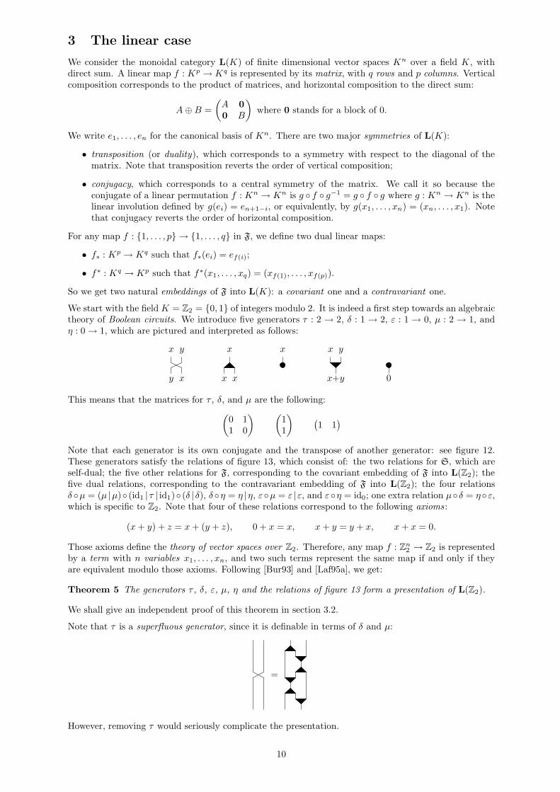
3 The linear case

We consider the monoidal category L(K) of finite dimensional vector spaces Kn over a field K, withdirect sum. A linear map f : Kp → Kq is represented by its matrix, with q rows and p columns. Verticalcomposition corresponds to the product of matrices, and horizontal composition to the direct sum:

A⊕B =

(A 0

0 B

)where 0 stands for a block of 0.

We write e1, . . . , en for the canonical basis of Kn. There are two major symmetries of L(K):

• transposition (or duality), which corresponds to a symmetry with respect to the diagonal of thematrix. Note that transposition reverts the order of vertical composition;

• conjugacy, which corresponds to a central symmetry of the matrix. We call it so because theconjugate of a linear permutation f : Kn → Kn is g ◦ f ◦ g−1 = g ◦ f ◦ g where g : Kn → Kn is thelinear involution defined by g(ei) = en+1−i, or equivalently, by g(x1, . . . , xn) = (xn, . . . , x1). Notethat conjugacy reverts the order of horizontal composition.

For any map f : {1, . . . , p} → {1, . . . , q} in F, we define two dual linear maps:

• f∗ : Kp → Kq such that f∗(ei) = ef(i);

• f∗ : Kq → Kp such that f∗(x1, . . . , xq) = (xf(1), . . . , xf(p)).

So we get two natural embeddings of F into L(K): a covariant one and a contravariant one.

We start with the field K = Z2 = {0, 1} of integers modulo 2. It is indeed a first step towards an algebraictheory of Boolean circuits. We introduce five generators τ : 2 → 2, δ : 1 → 2, ε : 1 → 0, µ : 2 → 1, andη : 0 → 1, which are pictured and interpreted as follows:

y x

x y

x+y

x yx

x x

x

0

This means that the matrices for τ , δ, and µ are the following:

(0 11 0

) (11

) (1 1

)

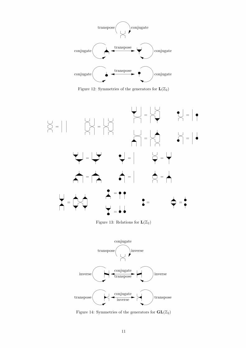
Note that each generator is its own conjugate and the transpose of another generator: see figure 12.These generators satisfy the relations of figure 13, which consist of: the two relations for S, which areself-dual; the five other relations for F, corresponding to the covariant embedding of F into L(Z2); thefive dual relations, corresponding to the contravariant embedding of F into L(Z2); the four relationsδ ◦µ = (µ |µ)◦ (id1 | τ | id1)◦ (δ |δ), δ ◦η = η |η, ε◦µ = ε |ε, and ε◦η = id0; one extra relation µ◦ δ = η ◦ε,which is specific to Z2. Note that four of these relations correspond to the following axioms :

(x+ y) + z = x+ (y + z), 0 + x = x, x+ y = y + x, x+ x = 0.

Those axioms define the theory of vector spaces over Z2. Therefore, any map f : Zn2 → Z2 is represented

by a term with n variables x1, . . . , xn, and two such terms represent the same map if and only if theyare equivalent modulo those axioms. Following [Bur93] and [Laf95a], we get:

Theorem 5 The generators τ , δ, ε, µ, η and the relations of figure 13 form a presentation of L(Z2).

We shall give an independent proof of this theorem in section 3.2.

Note that τ is a superfluous generator, since it is definable in terms of δ and µ:

=

However, removing τ would seriously complicate the presentation.

10

conjugatetranspose

transposeconjugate conjugate

transposeconjugate conjugate

Figure 12: Symmetries of the generators for L(Z2)

==

= =

= =

===

= ==

= = =

=

=

Figure 13: Relations for L(Z2)

inversetranspose

conjugate

conjugate

transposeinverse inverse

conjugate

inversetranspose transpose

Figure 14: Symmetries of the generators for GL(Z2)

11

3.1 Linear permutations

Let GL(K) be the monoidal subcategory of L(K) whose morphisms are linear permutations. In this case,there is an extra symmetry, inversion, which reverts the order of vertical composition.

Note that any α : 2 → 2 defines elementary operations on matrices:

• Multiplying ψ : p → q by idi−1 | α | idq−i−1 on the left corresponds to an elementary operation onrows i and i+ 1 of the matrix. In that case, we say that we apply α to rows i and i+ 1.

• Multiplying ψ : p→ q by idj−1 |α | idp−j−1 on the right corresponds to an elementary operation oncolumns j and j + 1 of the matrix. In that case, we say that we apply α to columns j and j + 1.

Again, we consider the case of Z2. Apart from id2 and τ , there are four linear permutations of Z22:

x x+y

x y x y

x+y y x+y x

x y x y

y x+y

The corresponding matrices are the following:

(1 01 1

) (1 10 1

) (1 11 0

) (0 11 1

)

The symmetries are given in figure 14. Of course, each of them is definable in terms of τ , δ, and µ:

= = ==

But δ and µ are not permutations. In fact, GL(Z2) is generated by τ and any of the four above generators,for instance the third one, that we call κ. The other ones are indeed superfluous:

== =

Theorem 6 The generators τ , κ, and the six relations of figure 15 form a presentation of GL(Z2).

To show this, we need an extended notion of stairs :

· · ·

· · ·· · ·

· · ·

· · ·

· · ·

oris or

Of course, there is a dual notion of antistairs. We consider a first notion of canonical form:

· · ·

· · ·

· · · · · ·

· · ·

· · ·

· · ·

is void or

It is obtained by the following algorithm, which applies to any invertible matrix A of order n:

1. Consider the last row of A, and let j be the last index for which the coefficient is 1.

2. While j > 1, apply τ or κ−1 to columns j − 1 and j, so that this index becomes j − 1.

3. By construction, the last row is now(1 0 · · · 0

). So, if we consider the first column, n is the

last index i for which the coefficient is 1.

4. While i > 1, apply τ or κ−1 to rows i − 1 and i, so that this index becomes i − 1, and row i − 1becomes

(1 0 · · · 0

).

12

To sum up, we have made the following transformations:

∗ · · · ∗ ∗ ∗ · · · ∗...

......

......

∗ · · · ∗ ∗ ∗ · · · ∗∗ · · · ∗ 1 0 · · · 0

−→

∗ ∗ · · · ∗...

......

∗ ∗ · · · ∗1 0 · · · 0

−→

1 0 · · · 00 ∗ · · · ∗...

......

0 ∗ · · · ∗

In particular, we get a matrix of the form 1 ⊕ A′, where A′ is an invertible matrix of order n − 1. Theantistairs are given by step 2, the stairs by step 4, and the rest of the canonical form is obtained byapplying the algorithm to the matrix A′. See figure 16 for an example.

As a by-product, we get a simple algorithm for inverting matrices: see appendix B. It is easy to see thatthis canonical form is unique, but it is not suitable for our purpose, because the stairs and the antistairsare far away. For that reason, we shall use an alternative notion of canonical form:

· · ·

· · ·

· · ·

· · ·

· · ·

· · ·

· · ·

is void or

Lemma 9 Any linear permutation f : Kn → Kn is represented by a unique canonical form.

This is proved by induction on n, using the following algorithm, which applies to any invertible matrixA of order n:

1. The matrix obtained by forgetting the first column of A is of rank n − 1. Since 1 is the uniqueinvertible element of Z2, there is a unique non-trivial linear relation a1u1 + · · · + anun = 0, whereu1, . . . , un are the rows of this truncated matrix. Let i be the first index such that ai = 1.

2. While i < n, apply τ or κ−1 to rows i and i+ 1 of A, so that this index becomes i+ 1.

3. By construction, the last row is now(1 0 · · · 0

).

4. Proceed as in the previous algorithm.

To sum up, we have made the following transformations:

∗ ∗ · · · ∗...

......

∗ ∗ · · · ∗∗ ∗ · · · ∗∗ ∗ · · · ∗...

......

∗ ∗ · · · ∗

0...01∗...∗

−→

∗ ∗ · · · ∗

......

...

∗ ∗ · · · ∗1 0 · · · 0

0

...

01

−→

1 0 · · · 00 ∗ · · · ∗

......

...

0 ∗ · · · ∗

The extra column on the right contains a1, . . . , an. Again, we get a matrix of the form 1⊕A′. This A′ isobtained by removing the first column and one row of the original matrix. See figure 17 for an example.

In figure 18, we introduce two groups of rules for the following transformations:

or

Those fourteen rules are derivable from the six relations of figure 15. Indeed, five rules are already in thepresentation, five more are derived in figure 19, and we get three more by duality. It remains to showthat the last rule of figure 18 is derivable from the presentation. This is done in figure 20, using thesuperfluous generator κ2, which is both the inverse and the conjugate of κ:

=

13

== =

= = =

Figure 15: Relations for GL(Z2)

0011

1000

1101

10

01

0011

10

01

1101

1000

1 1 0 01 1 1 1

0 1 0 11 0 0 0

1 1 1 1

0 1 0 1

1 0 0 00 1 0 0

1 1 1 11 1 0 00 1 0 11 0 0 0

111

100

101

111

101

100

1 0 10 1 01 0 0

1 0 11 0 00 1 0

0 11 0

1 00 1

0 1 0

1 0 00 0 1

0 1 0 1

1 0 0 00 1 1 10 1 0 0

Figure 16: Computing the first canonical form of a matrix in GL(Z2)

0 1 1 11 0 0 11 0 0 00 0 1 0

0 1 1 1

0 0 1 00 0 0 11 0 0 0

0 0 1 00 0 0 10 1 1 11 0 0 00

101

0 1 1 10 0 1 01 0 0 11 0 1 0

0

1

01

0 1 1 1

1 0 1 0

1 0 0 10 0 1 0

0

1

00

0 1 1 11 0 0 11 0 1 01 0 0 0

00 11 0 0

1 00 1 00

1 0 000 1

111

1 1 100 11 00

0

11

1 00

00 11 1 0

0

10

00 11 00

1 0 0

1 00 1

011 0

0 1

Figure 17: Computing the second canonical form of a matrix in GL(Z2)

14

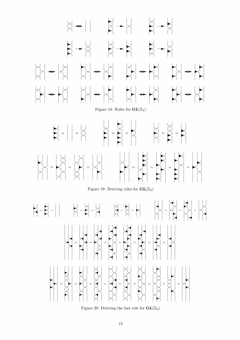
Figure 18: Rules for GL(Z2)

= = = = = = =

= = = = = =

Figure 19: Deriving rules for GL(Z2)

= = = = = =

= == = = = =

= = = = = = = = =

= = =

Figure 20: Deriving the last rule for GL(Z2)

15

Lemma 10 For any diagram φ, we have the following commutations:

· · ·

· · ·φ· · ·

φ· · ·

· · ·

· · ·φ· · ·

· · ·

· · · · · ·

φ· · ·

· · ·

This is easily proved by induction on the size m of φ, using the second group of rules. Of course, thestairs (respectively the antistairs) may be changed by this commutation.

Lemma 11 Any diagram φ : n→ n reduces to a canonical form φ by the rules of figure 18.

This is proved by double induction on n and the size m of φ:

• If m = 0, then φ = idn, which reduces to a canonical form. This is proved by induction on n, usingthe first rule:

· · ·

· · ·

· · ·

· · ·· · ·

· · ·

· · ·

· · ·

• If m ≥ 1, then φ = ξ ◦ ψ where ξ is an elementary diagram and ψ is a diagram of size m− 1 whichreduces to a canonical form ψ by induction hypothesis. Therefore, φ reduces to ξ ◦ ψ and there arefour possible cases (figure 21): in the first case, we use the second group of rules and the inductionhypothesis for n − 1; in the second case, we get a canonical form; in the third case, we use thecrucial transformation of figure 22, which itself uses lemma 10 and the first group of rules, and theinduction hypothesis for n − 1; in the fourth case, we use the second group of rules twice and theinduction hypothesis for n− 1.

Theorem 6 follows from lemma 9 and lemma 11.

Note that the rewrite system of figure 18 is not terminating. It is easy to give an alternative systemsuch that identity diagrams are in canonical form, but the existence of a terminating rewrite system forGL(Z2) is an open question. Indeed, it is essential that the rules of the second group are used in bothdirections: one for stairs and one for antistairs. Furthermore, the fact that we need both stairs andantistairs does not rely on our choice of generators. Indeed, even if we take all linear permutations of Z2

2

as generators, there are linear permutations of Z32 which cannot be decomposed as follows:

In other words, there are invertible matrices of order 3 which are not of the form (1⊕A)(B ⊕ 1)(1⊕C).Here is an example:

1 1 01 0 10 1 0

Finally, note that τ is almost a superfluous generator, since τ | id1 and id1 | τ are definable in terms of κ:

= =

This means that τ is only necessary in dimension 2, but again, removing it would seriously complicatethe presentation.

16

· · ·

· · ·

· · ·

· · · · · · · · ·

· · ·

· · ·

· · · · · ·

· · ·

· · ·

· · ·

· · · · · ·· · ·

· · ·

· · ·

· · ·

· · · · · ·

· · ·

Figure 21: The four cases of lemma 11

· · ·

· · ·

· · ·

· · ·· · ·

· · ·

· · ·

· · ·

· · ·

· · ·

· · ·

· · ·

· · ·

· · ·

· · ·

· · ·

· · ·

· · ·

· · ·

· · ·

· · ·

· · ·

· · ·· · ·

· · ·

· · ·

· · ·

· · ·

· · ·

· · ·

· · ·

· · ·

· · ·

· · ·

· · ·

· · ·

· · ·

· · ·

· · ·

· · ·

· · ·

· · ·

· · ·

· · ·

· · ·

· · ·

· · ·

· · ·

· · ·

· · ·

· · ·

· · ·

· · · · · ·

· · ·

· · ·

· · ·

· · ·

· · ·

· · ·

· · ·

· · ·

· · ·

Figure 22: Crucial transformation for the third case of lemma 11

17

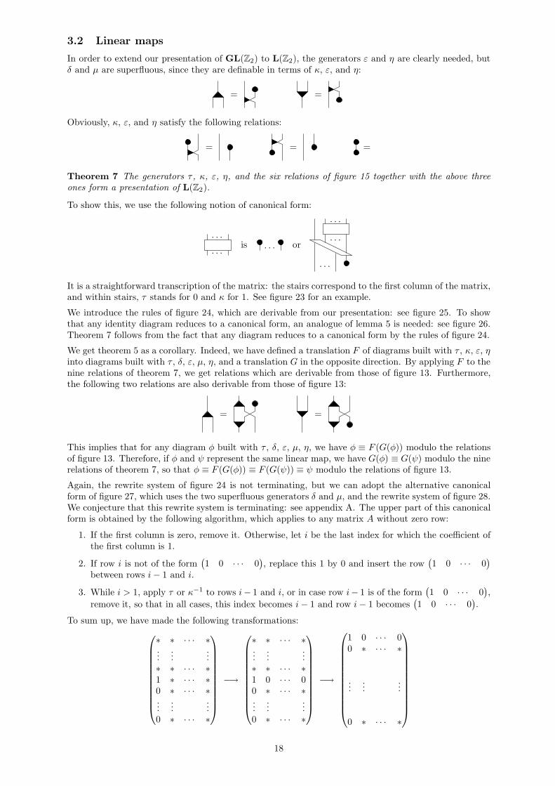
3.2 Linear maps

In order to extend our presentation of GL(Z2) to L(Z2), the generators ε and η are clearly needed, butδ and µ are superfluous, since they are definable in terms of κ, ε, and η:

==

Obviously, κ, ε, and η satisfy the following relations:

= = =

Theorem 7 The generators τ , κ, ε, η, and the six relations of figure 15 together with the above threeones form a presentation of L(Z2).

To show this, we use the following notion of canonical form:

· · ·· · ·

· · ·

· · ·

· · ·

· · ·oris

It is a straightforward transcription of the matrix: the stairs correspond to the first column of the matrix,and within stairs, τ stands for 0 and κ for 1. See figure 23 for an example.

We introduce the rules of figure 24, which are derivable from our presentation: see figure 25. To showthat any identity diagram reduces to a canonical form, an analogue of lemma 5 is needed: see figure 26.Theorem 7 follows from the fact that any diagram reduces to a canonical form by the rules of figure 24.

We get theorem 5 as a corollary. Indeed, we have defined a translation F of diagrams built with τ , κ, ε, ηinto diagrams built with τ , δ, ε, µ, η, and a translation G in the opposite direction. By applying F to thenine relations of theorem 7, we get relations which are derivable from those of figure 13. Furthermore,the following two relations are also derivable from those of figure 13:

= =

This implies that for any diagram φ built with τ , δ, ε, µ, η, we have φ ≡ F (G(φ)) modulo the relationsof figure 13. Therefore, if φ and ψ represent the same linear map, we have G(φ) ≡ G(ψ) modulo the ninerelations of theorem 7, so that φ ≡ F (G(φ)) ≡ F (G(ψ)) ≡ ψ modulo the relations of figure 13.

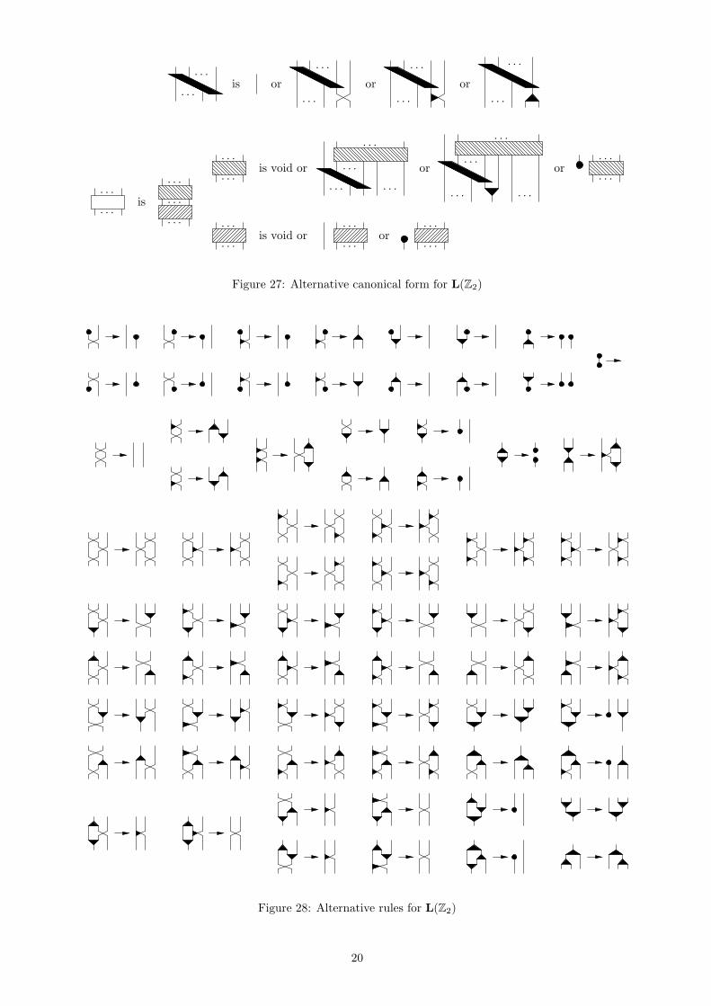
Again, the rewrite system of figure 24 is not terminating, but we can adopt the alternative canonicalform of figure 27, which uses the two superfluous generators δ and µ, and the rewrite system of figure 28.We conjecture that this rewrite system is terminating: see appendix A. The upper part of this canonicalform is obtained by the following algorithm, which applies to any matrix A without zero row:

1. If the first column is zero, remove it. Otherwise, let i be the last index for which the coefficient ofthe first column is 1.

2. If row i is not of the form(1 0 · · · 0

), replace this 1 by 0 and insert the row

(1 0 · · · 0

)

between rows i− 1 and i.

3. While i > 1, apply τ or κ−1 to rows i− 1 and i, or in case row i− 1 is of the form(1 0 · · · 0

),

remove it, so that in all cases, this index becomes i− 1 and row i− 1 becomes(1 0 · · · 0

).

To sum up, we have made the following transformations:

∗ ∗ · · · ∗...

......

∗ ∗ · · · ∗1 ∗ · · · ∗0 ∗ · · · ∗...

......

0 ∗ · · · ∗

−→

∗ ∗ · · · ∗...

......

∗ ∗ · · · ∗1 0 · · · 00 ∗ · · · ∗...

......

0 ∗ · · · ∗

−→

1 0 · · · 00 ∗ · · · ∗

......

...

0 ∗ · · · ∗

18

111

001

100

101

Figure 23: The canonical forms of a matrix in L(Z2)

Figure 24: Rules for L(Z2)

=== = = === =

==

Figure 25: Deriving rules for L(Z2)

· · ·

· · ·

· · ·

· · ·

· · ·

· · · · · ·

· · ·

· · · · · ·

· · ·

· · ·

· · ·

Figure 26: Expansion of identities for L(Z2)

19

· · ·

· · ·· · ·

· · ·

· · ·

· · · · · ·

· · ·

oris or or

· · ·

· · ·

· · · · · ·

· · ·

· · ·

· · ·

· · ·· · ·

· · ·

· · ·

· · ·is void or or or

· · ·

· · ·

· · ·

· · ·

· · ·

· · ·is void or or

· · ·

· · ·· · ·

· · ·

· · ·

is

Figure 27: Alternative canonical form for L(Z2)

Figure 28: Alternative rules for L(Z2)

20

In particular, we get a matrix of the form 1⊕A′, and by construction, A′ has no zero row. The µ cell (ifany) is given by step 2, the (generalized) stairs by step 3, and the rest of the canonical form is obtainedby applying the algorithm to the matrix A′. See figure 23 for an example.

Note that the rewrite system of figure 28 extends the one of figure 9. Furthermore, it is self-dual, so thatthe canonical form of the dual is always the dual of the canonical form. This may not be clear from thegrammar of figure 27, but remember that we have an implicit commutation rule.

Note also that the canonical form of a linear permutation may contain the generators δ and µ, which arenot permutations, as in the following example:

Instead, we can generalize the first canonical form of linear permutations as follows:

· · ·

· · ·· · ·

· · · · · ·

· · ·

· · ·

· · ·

· · ·

· · ·oris or

This canonical form is obtained by the same algorithm as in the case of linear permutations, except thatthe last row may be zero, and one may end with a degenerate matrix. See figure 23 for an example. Thisalgorithm can also be used to compute the rank of a matrix. Note the following points:

• The canonical form of a linear permutation contains only τ and κ.

• The canonical form of a linear surjection contains only τ , κ, and ε.

• The canonical form of a linear injection contains only τ , κ, and η.

In particular, the monoidal subcategory Lsurj(Z2) of L(Z2) whose morphisms are linear surjections isgenerated by τ , κ, and ε. We have already seen that these generators satisfy the following relations:

= =

Theorem 8 The generators τ , κ, ε, and the six relations of figure 15 together with the above two onesform a presentation of Lsurj(Z2).

By duality, we get a presentation of the monoidal subcategory Linj(Z2) of L(Z2) whose morphisms arelinear injections by τ , κ, η, and the six relations of figure 15 together with the dual of the above ones.

To show theorem 8, we consider the following canonical form of linear surjections, which generalizes thesecond canonical form of linear permutations:

· · ·

· · ·

· · ·

· · ·

· · ·

· · ·

· · ·

· · ·

· · ·

· · ·is void or or

It is obtained by the following algorithm, which applies to any matrix A with q independent rows:

1. The matrix obtained by forgetting the first column of A is of rank q − 1 or q.

2. If the rank is q, remove this first column. Otherwise, there is a unique non-trivial linear relationa1u1 + · · · + anun = 0, where u1, . . . , un are the rows of this truncated matrix.

3. Proceed as in the case of linear permutations.

21

We get a canonical form of the second type if the rank is q − 1, or of the third type if the rank is q, andin that case, the stairs corresponds to the first column of the matrix. See figure 29 for an example.

In figure 30, we introduce rules for the following transformations:

or

Those rules are derivable from the six relations of figure 15 together with the above two ones: see figure 31.

Theorem 8 follows from the fact that any diagram reduces to a canonical form by the rules of figure 18together with those of figure 30. To show this, we proceed as in the case of linear permutations, usingthe crucial transformation of figure 32.

The canonical form of linear surjections can be generalized to linear maps: see figure 33. The bottompart of this canonical form is obtained by the following algorithm, which takes any system u1, . . . , uq andreturns a free subsystem of the same rank:

1. Apply the algorithm to u2, . . . , uq: it returns a free subsystem v1, . . . , vn.

2. If u1 is independent of v1, . . . , vn, return u1, v1, . . . , vn. Otherwise, return v1, . . . , vn.

This algorithm is applied to the rows of the matrix. One gets a canonical form of the second type if u1 isindependent of v1, . . . , vn, or of the third type if u1 = a1v1 + · · · + anvn, and in that case, the antistairsare given by the coefficients a1, . . . , an. In both cases, the rest of the canonical form is given by step 1.Finally, the algorithm returns a matrix with independent rows, corresponding to a linear surjection, fromwhich one gets the upper part of the canonical form. See figure 35 for an example.

The canonical form of figure 33 corresponds to the unique decomposition of any linear map f : Zp2 → Z

q2

into a linear surjection g : Zp2 → Zn

2 followed by a monotone linear injection h : Zn2 → Z

q2, where n is the

rank of f . Here, we assume that Zn2 is equipped with the following antilexicographical ordering:

(0, x2, . . . , xn) < (1, x2, . . . , xn), (x1, . . . , xn) < (y1, . . . , yn) whenever (x2, . . . , xn) < (y2, . . . , yn).

It is indeed easy to see that the bottom part of a canonical form corresponds to a monotone linearinjection. The converse is proved by induction on q, using the following lemma:

Lemma 12 Let A be the matrix of a monotone linear injection f : Zp2 → Z

q2 and let B be the matrix

obtained by removing the first row of A. Then B is the matrix of a monotone linear injection or A is ofthe form 1 ⊕ C where C is the matrix of a monotone linear injection.

By definition of the ordering, B is indeed the matrix of a monotone linear map g : Zp2 → Z

q−12 . If g is

not injective, then g(u) = 0 for some u 6= 0 in Zp2. Since f is injective, f(u) = e1, which is the smallest

element after 0 in Zq2. Since f is a monotone injection, u = e1. Now, if j > 1, then ej < e1 + ej and

f(ej) < f(e1+ej) = f(e1)+f(ej) = e1+f(ej), so that the first component of f(ej) must be 0. Therefore,A is of the form 1 ⊕ C, and it is easy to check that C is the matrix of a monotone linear injection.

Monotone linear injections form a monoidal subcategory of Linj(Z2) which is not finitely generated. Infact, it is generated by all maps of the form f(x1, . . . , xn) = (a1x1 + · · · + anxn, x1, . . . , xn), which arerepresented by diagrams of the following form:

· · ·

· · ·

Note also that if we apply the above decomposition to a linear injection, we get a linear permutationfollowed by a monotone linear injection. This means that monotone linear injections provide a canonicalchoice of basis for subspaces of Zn

2 .

There is a dual notion of comonotone linear surjection. Any linear map can be uniquely decomposedinto a comonotone linear surjection followed by a linear injection. Again, if we apply this decompositionto a linear surjection, we get a comonotone linear surjection followed by a linear permutation. In fact,the comonotone linear surjections coincide with the conjugate of linear surjections whose matrices are inrow-reduced echelon form. This row-reduced echelon form is just what we get when we apply the Gaussalgorithm to solve a linear system.

Finally, any linear map can be uniquely decomposed into a comonotone linear surjection followed bya linear permutation followed by a monotone linear injection. This decomposition corresponds to thecanonical form of figure 34. See figure 35 for an example.

22

111

001

100

101

Figure 29: The canonical form of a matrix in Lsurj(Z2)

Figure 30: Extra rules for Lsurj(Z2)

= = = = == = =

Figure 31: Deriving rules for Lsurj(Z2)

· · ·

· · · · · ·

· · · · · ·

· · · · · ·

· · · · · ·

· · ·

· · · · · ·

· · · · · ·

· · ·· · ·

· · · · · ·

· · · · · ·

· · ·

· · · · · ·

· · · · · ·

· · ·· · ·

· · ·

· · ·

· · ·

· · · · · ·

· · ·· · ·

· · · · · ·

· · · · · ·

· · · · · ·

· · ·

· · · · · ·

· · ·

· · ·

· · ·

· · ·

· · ·· · ·

· · ·· · ·

· · · · · ·

· · ·· · ·

· · ·

· · ·

· · ·

· · ·

· · ·

· · ·

· · ·

· · ·

· · ·

· · ·

· · ·

· · ·

· · ·

· · ·

· · ·

Figure 32: Crucial transformation for Lsurj(Z2)

23

· · ·

· · ·

· · ·

· · ·

· · ·

· · ·

· · ·· · ·

· · ·

· · ·is void or or

· · ·

· · ·

· · ·

· · ·

· · ·

· · ·

· · ·

is void or or

· · ·

· · ·· · ·

· · ·

· · ·

is

Figure 33: Another canonical form for L(Z2)

· · ·

· · ·

· · ·

· · ·

· · ·

· · ·is

· · ·

· · ·

· · ·

· · ·

· · ·

· · ·

· · ·

is void or or

· · ·

· · ·

· · ·

· · ·

· · ·

· · ·

· · ·

is void or

· · ·

· · ·

· · ·

· · ·

· · ·

· · ·

· · ·is void or or

Figure 34: Yet another canonical form for L(Z2)

0 0 0 0

1 101

0 01 1

1 0 0 0

1 0 1 1

Figure 35: Other canonical forms of a matrix in L(Z2)

24

3.3 Arbitrary field

The results of the previous sections can be generalized to an arbitrary field K. First we introduce agenerator Ha : 1 → 1 for each a ∈ K. It is pictured and interpreted as follows:

ax

x

a

In particular, we write σ for H−1, which is pictured and interpreted as follows:

x

−x

The presentation of L(K) is the one of figure 13, where the last relation is replaced by the nine relationsof figure 36. The last six relations correspond to the following axioms for vector spaces:

a(x+ y) = ax+ ay, a0 = 0, a(bx) = (ab)x, 1x = x, (a+ b)x = ax+ bx, 0x = 0.

Note that H0 and H1 are superfluous generators. Furthermore, in the case of a finite field, it is well knownthat the multiplicative group of invertible elements is cyclic, so that the Ha for a 6= 0 are definable interms of a single one. Note also that τ is always definable in terms of δ, µ, and σ:

=

For GL(K), we keep the Ha for a 6= 0, and we introduce a new generator Ka : 2 → 2 for each a ∈ K,which is pictured and interpreted as follows:

x y

a

xax+y

In particular, we write τ for K0 and κ for K1 as in the case of Z2:

x+y x

x yx y

y x

Note that the Ka for a 6= 0 are definable in terms of κ and the Ha:

a

1/a

a

a

1/a

= =

Stairs and antistairs are built with the Ka, and the second canonical form is generalized as follows:

· · ·

· · ·

· · ·

· · ·

· · ·

· · ·

· · ·

is void or

Any diagram built with the Ha for a 6= 0 and the Ka reduces to such a canonical form by the rules offigure 37. From this, it is possible to get a presentation of GL(K) with τ , κ, and the Ha for a 6= 0 asgenerators. Again, a single Ha is needed in the case of a finite field.

25

3.4 Isometries

Finally, we consider the monoidal subcategory O of GL(R) whose morphisms are isometries. An isometryis a linear map f : R

n → Rn which preserves the Euclidean metrics of R

n. The matrix of an isometryis called an orthogonal matrix : its columns form an orthonormal basis, that is a system u1, . . . , un suchthat each ui has length 1, and ui is orthogonal to uj for j 6= i. Note that if all coefficients of u1 are zero,but the first one, then the matrix is of the form ±1⊕A where A is an orthogonal matrix of order n− 1.

Apart from the identity, σ is the only isometry of R. The isometries of R2 are rotations or symmetries.So we introduce a generator Rα : 2 → 2 for each α ∈ R, which is pictured as follows:

α

It stands for the rotation of angle α, whose matrix is

(cosα − sinαsinα cosα

).

Symmetries are definable in terms of the Rα and σ. For instance, τ can be decomposed as follows:

π/2=

Note also that Rπ is definable in terms of σ:

π =

Therefore, we shall only use Rα for α ∈ ]0, π[. Stairs are built with those Rα, and there is a simple notionof canonical form which is similar to the canonical form of permutations in the basic case:

· · ·

· · ·· · ·

· · ·· · ·

· · ·

· · ·

· · ·· · ·

· · ·is void or or

It is obtained by the following algorithm, which applies to any orthogonal matrix A of order n:

1. Consider the first column of A, and let i be the last index for which the coefficient is 6= 0.

2. While i > 1, apply R−1α to rows i − 1 and i, so that this index becomes i − 1. For that purpose,

choose α such that cotα = ai−1/ai, where aj stands for the first coefficient of row j.

By the previous remark, we get a matrix of the form ±1 ⊕A′ where A′ is an orthogonal matrix of ordern − 1. The type of the canonical form is given by the sign ±1, the stairs by step 2, and the rest of thecanonical form is obtained by applying the algorithm to the matrix A′.

In dimension 3, we get the canonical form of figure 38. The parameters α, β, γ ∈ ]0, π[ which appear inthe bottom part of this canonical form are called Euler angles. In the first case, where three angles areactually needed, we say that the decomposition is generic.

Lemma 13 If α, β, γ ∈ ]0, π[, there are α′, β′, γ′ ∈ ]0, π[ such that (Rγ | id1) ◦ (id1 | Rβ) ◦ (Rα | id1) is ofthe form (id1 | Rα′) ◦ (Rβ′ | id1) ◦ (id1 | Rγ′).

α

β

γ

γ′

β′

α′

=

The parameters α′, β′, γ′ are given by the above algorithm. In this case, it happens that no σ appears inthe canonical form, and the decomposition is generic. Obviously, the generators satisfy the extra relationsof figure 39. Using the same argument as for theorem 1, one proves:

Theorem 9 The generators σ, Rα for α ∈ ]0, π[, and the relations of lemma 13 together with those offigure 39 form a presentation of O.

Similarly, it is possible to get a presentation of the monoidal subcategory SO of O whose morphismsare rotations with the Rα for α ∈ ]0, 2π[ as generators. All this can be easily generalized to get apresentation of the monoidal subcategory U of GL(C) whose morphisms are unitary maps and similarlyfor the monoidal subcategory SU of U whose morphisms are special unitary maps. Using this, one getspresentations for the groups On, SOn, Un, and SUn.

26

aba

b= 1 = a ba+b = 0 =

aa

=

a=

aa a

=

a aa

=a

=

Figure 36: Extra relations for L(K)

a

b

b

ab b

ab

a

b1

a

bab

a

b

c

c

a

b+ac

b

a

a+b

a

b

c

b

a+1/b

c+1/b

−1/bb 6= 0

Figure 37: Rules for GL(K)

orisis

α

γ

βα

β

α

βα αis or or or or or

Figure 38: Canonical form for O3

=π−α

α=

α

π−α=

α

βα+β=

α+β < π

Figure 39: Extra relations for O

27

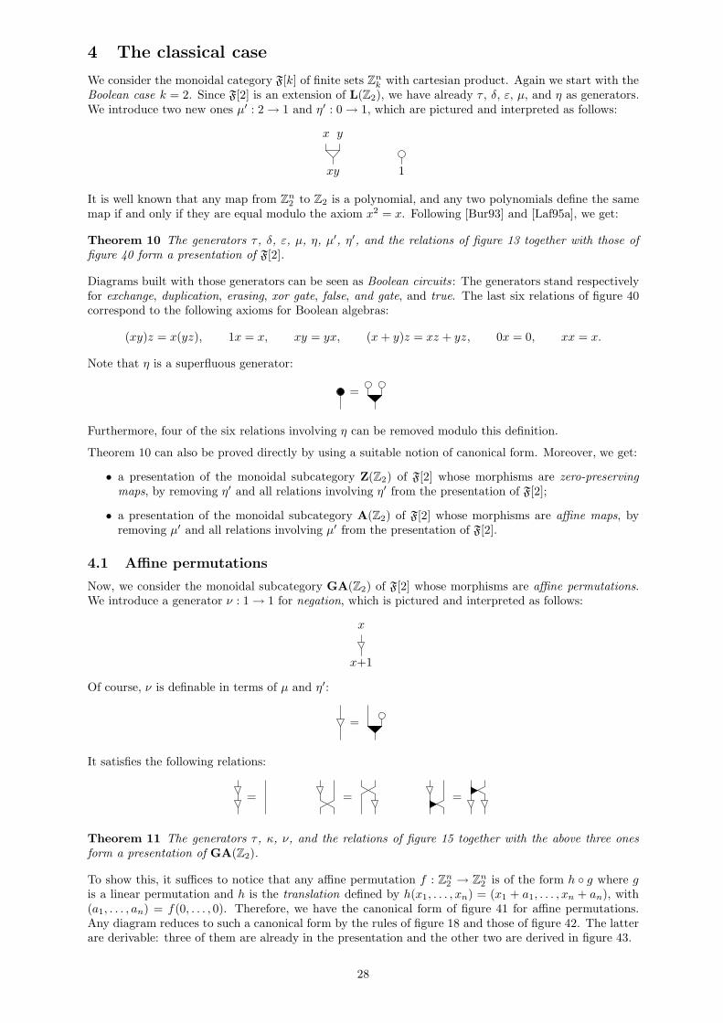
4 The classical case

We consider the monoidal category F[k] of finite sets Znk with cartesian product. Again we start with the

Boolean case k = 2. Since F[2] is an extension of L(Z2), we have already τ , δ, ε, µ, and η as generators.We introduce two new ones µ′ : 2 → 1 and η′ : 0 → 1, which are pictured and interpreted as follows:

xy

x y

1

It is well known that any map from Zn2 to Z2 is a polynomial, and any two polynomials define the same

map if and only if they are equal modulo the axiom x2 = x. Following [Bur93] and [Laf95a], we get:

Theorem 10 The generators τ , δ, ε, µ, η, µ′, η′, and the relations of figure 13 together with those offigure 40 form a presentation of F[2].

Diagrams built with those generators can be seen as Boolean circuits : The generators stand respectivelyfor exchange, duplication, erasing, xor gate, false, and gate, and true. The last six relations of figure 40correspond to the following axioms for Boolean algebras:

(xy)z = x(yz), 1x = x, xy = yx, (x + y)z = xz + yz, 0x = 0, xx = x.

Note that η is a superfluous generator:

=

Furthermore, four of the six relations involving η can be removed modulo this definition.

Theorem 10 can also be proved directly by using a suitable notion of canonical form. Moreover, we get:

• a presentation of the monoidal subcategory Z(Z2) of F[2] whose morphisms are zero-preservingmaps, by removing η′ and all relations involving η′ from the presentation of F[2];

• a presentation of the monoidal subcategory A(Z2) of F[2] whose morphisms are affine maps, byremoving µ′ and all relations involving µ′ from the presentation of F[2].

4.1 Affine permutations

Now, we consider the monoidal subcategory GA(Z2) of F[2] whose morphisms are affine permutations.We introduce a generator ν : 1 → 1 for negation, which is pictured and interpreted as follows:

x

x+1

Of course, ν is definable in terms of µ and η′:

=

It satisfies the following relations:

= = =

Theorem 11 The generators τ , κ, ν, and the relations of figure 15 together with the above three onesform a presentation of GA(Z2).

To show this, it suffices to notice that any affine permutation f : Zn2 → Zn

2 is of the form h ◦ g where gis a linear permutation and h is the translation defined by h(x1, . . . , xn) = (x1 + a1, . . . , xn + an), with(a1, . . . , an) = f(0, . . . , 0). Therefore, we have the canonical form of figure 41 for affine permutations.Any diagram reduces to such a canonical form by the rules of figure 18 and those of figure 42. The latterare derivable: three of them are already in the presentation and the other two are derived in figure 43.

28

= = =

= = =

= = =

=

=

=

Figure 40: Extra relations for F[2]

· · ·

· · ·· · ·

· · ·

· · ·

is

· · ·

· · ·

· · ·

· · ·

· · ·

· · ·is void or or

· · ·

· · ·

· · ·

· · ·

· · ·

· · ·

· · ·

is void or

Figure 41: Canonical form for GA(Z2)

Figure 42: Extra rules for GA(Z2)

= = =

= = = = = = = ==

Figure 43: Deriving rules for GA(Z2)

29

4.2 Classical permutations

It is easy to see that, for n ≤ 2, any permutation of Zn2 is affine, but it is not the case for n = 3. So we

introduce the 3-bit Toffoli gate T3 : 3 → 3, which is pictured and interpreted as follows:

T3

x y z

z+xyx y

This T3 is an involution: It corresponds to the transposition of Z32 which exchanges (1, 1, 0) with (1, 1, 1).

More generally, we introduce the n-bit Toffoli gate Tn : n → n for each n ≥ 1, corresponding to thetransposition of Zn

2 which exchanges (1, . . . , 1, 0) with (1, . . . , 1, 1). For instance, T1 is the negation ν andT2 is the linear involution τ ◦ κ.

It happens that the monoidal subcategory S[2] of F[2] whose morphisms are permutations is not finitelygenerated. This follows from the following remark:

Lemma 14 If f is a finite permutation, then f × idZ2and idZ2

× f are even permutations.

Indeed, for any decomposition of f into n transpositions, we get a decomposition of f × idZ2into 2n

transpositions, and similarly for idZ2× f .

Now, assume that we have cells α1 : p1 → p1, . . . , αk : pk → pk in S[2] and let m = max(p1, . . . , pk).Then any diagram φ : n→ n built with those generators represents an even permutation of Z

n2 whenever

n > m. To show this, it suffices to consider the case of an elementary diagram, and the lemma applies inthat case. In particular, the odd permutation Tm+1 is not definable in terms of α1, . . . , αk. Therefore,we consider the monoidal subcategory A[2] of S[2] whose morphisms are even permutations.

Theorem 12 A[2] is contained in the monoidal subcategory of S[2] generated by τ , T1, T2, and T3.

These generators represent transpositions, which are not in A[2], but we have the following corollaries:

Corollary 1 A[2] is finitely generated.

Indeed, there are finitely many even permutations of Zn2 with n ≤ 3, and by the theorem, any even

permutation of Zn2 with n ≥ 4 is definable in terms of τ | id1, id1 | τ , Ti | id1, and id1 | Ti for i = 1, 2, 3.

In fact, three generators suffice: see [Mus97].

Corollary 2 S[2] is generated by τ and the Tn for n ≥ 1.

For any permutation f of Zn2 , it suffices apply the theorem to f if it is even, or to Tn ◦ f if it is odd.

Theorem 12 is proved in [Mus97], using the Fredkin gate F3 : 3 → 3 instead of T3: It corresponds to thetransposition of Z

32 which exchanges (1, 0, 1) with (1, 1, 0). This F3 is definable in terms of τ , T2, and T3:

F3 T3

T2

T2

=

The proof is based on the fact that any even permutation can be decomposed into 3-cycles. It does notuse any notion of canonical form for S[2] or A[2]. Therefore, it is not very helpful for getting presentationsof those monoidal categories. Of course, some obvious commutations are satisfied by the generators:

T3

T3=T2

T3

T3

T2

=T3

T3

T2

=T3

T3=

But it is clear that other relations are needed.

Finally, note that S[k] is not finitely generated whenever k is an even number, since we have an analogueof lemma 14. On the other hand, Peter Selinger showed that S[k] is finitely generated by unary andbinary gates whenever k is an odd number (private communication).

30

Acknowledgements

This paper is dedicated to Albert Burroni who inspired this theory. The author wish also to thank SergeBurckel, Julien Cassaigne, and Peter Selinger for fruitful interactions.

References

[Bur93] A. Burroni, Higher Dimensional Word Problem, Theoretical Computer Science 115, 1993,pp. 43–62.

[LP91] Y. Lafont, A. Proute, Church-Rosser property and homology of monoids, MathematicalStructures in Computer Science 1 (3), Cambridge University Press, 1991, pp. 297–326.

[Laf92] Y. Lafont, Penrose diagrams and 2-dimensional rewriting, Applications of Categories in Com-puter Science (ed. M.P. Fourman, P.T. Johnstone & A.M. Pitts), LMSLNS 177, CambridgeUniversity Press, 1992, pp. 191–201.

[Laf95a] Y. Lafont, Equational reasoning with 2-dimensional diagrams, Term Rewriting, Lecture Notesin Computer Science 909, Springer-Verlag, 1995, pp. 170-195.

[Laf95b] Y. Lafont, A new finiteness condition for monoids presented by complete rewriting systems(after Craig C. Squier), Journal of Pure and Applied Algebra 98, North-Holland, 1995, pp.229-244.

[Law63] F.L. Lawvere, Functorial Semantics of Algebraic Theories, Proc. Nat. Acad. Sci. USA, 1963.

[Mac71] S. Mac Lane, Categories for the Working Mathematician, GTM 5, Springer-Verlag, 1971.

[Mas97a] A. Massol, Minimality of the system of seven equations for the category of finite sets, Theo-retical Computer Science, 176, 1997, pp. 347–353.

[Mas97b] A. Massol, Calcul symbolique avec des diagrammes de Penrose, these de doctorat, Universited’Aix-Marseille II, 1997.

[Mus97] J. Musset, Generateurs et relations pour les circuits booleens reversibles, rapport de stage,Institut de Mathematiques de Luminy, preprint 97-32.1

[Squ87] C. C. Squier, Word problems and a homological finiteness condition for monoids, Journal ofPure and Applied Algebra, 49, 1987, pp. 201–217.

[SOK94] C. C. Squier, F. Otto, Y. Kobayashi, A finiteness condition for rewriting systems, Theo-retical Computer Science, 131, 1994, pp. 271–294.

1available on ftp://iml.univ-mrs.fr/pub/lafont/musset.ps.gz

31

A Rewriting

The theory of rewriting is well established in the case of words and in the case of terms. Following [Laf92],we explain how it can be generalized to diagrams. Detailed proofs will not be given here.

A.1 Rewrite rules

A rewrite system is given by a set of cells and a set of rules. Each rule of the system is of the form ρ→ ρ′

where ρ, ρ′ : p→ q are two diagrams built with the cells of the system:

ρ· · ·

· · ·

· · ·ρ′· · ·

If such a rule is given, and if φ : m → i + p + j and ψ : i + q + j → n are any diagrams, we writeψ ◦ (idi | ρ | idj) ◦ φ→ ψ ◦ (idi | ρ

′ | idj) ◦ φ. This is called an elementary reduction:

ρ· · ·

· · ·· · · · · ·

· · ·

· · ·

φ

ψ

ρ′· · ·

· · ·· · · · · ·

· · ·

· · ·

φ

ψ

We write →∗ for the iterated reduction, which is the reflexive transitive closure of →. Similarly, we write↔∗ for the reflexive transitive closure of ↔, which is itself the symmetric closure of →. Note that φ↔∗ ψwhen φ and ψ are equivalent modulo the rules (considered as relations).

We say that a diagram φ is reduced if there is no φ′ such that φ → φ′. We say that ψ is a reduced formof φ if φ→∗ ψ and ψ is reduced. Note that the commutation rule does not count as a reduction. For thequestion of finding canonical decompositions, independently of the rewrite rules, see [Mas97b].

A.2 Termination

A rewrite system is terminating (or noetherian) if there is no infinite reduction φ0 → φ1 → φ2 → φ3 → · · ·In other words, any reduction strategy terminates and leads to a reduced form.

Consider for instance the rewrite system of lemma 2 for S:

This system is terminating because the first rule moves one cell to the right and the second rule removestwo cells. To make this argument precise, we define the natural number ‖φ‖ for any diagram φ as follows:

• If ξ = idi | σ | idj is an elementary diagram, then ‖ξ‖ = j + 1.

• If φ = ξ1 ◦ · · · ◦ ξn where ξ1, . . . , ξn are elementary diagrams, then ‖φ‖ = ‖ξ1‖ + · · · + ‖ξn‖.

This definition does not depend on the decomposition of φ because the number of inputs of the generatorσ is the same as its number of outputs. Since we have ‖φ‖ > ‖φ′‖ whenever φ → φ′, the length of anyreduction starting from a diagram φ is bounded by ‖φ‖.

The rewrite system of figure 9 for F is also terminating, but the previous argument cannot be extended.Instead, we interpret any diagram φ : p → q as a strictly monotonic map [φ] : N∗p → N∗q, where N∗ isthe set of strictly positive integers, and N∗n is equipped with the following partial order (product order):

(x1, . . . , xn) ≤ (y1, . . . , yn) whenever x1 ≤ y1, . . . , xn ≤ yn.

It suffices to give the interpretation of each generator: see figure 44. For any strictly monotone mapsf, g : N∗p → N∗q, we write f < g if f(x1, . . . , xp) < g(x1, . . . , xp) for all (x1, . . . , xp) ∈ N∗p. This relationis compatible with horizontal and vertical composition, and we have [ρ] > [ρ′] for each rule ρ → ρ′: seefigure 45. Therefore, [φ] > [φ′] whenever φ → φ′. Finally, the length of any reduction starting from adiagram φ is bounded by n1 + · · · + nq where (n1, . . . , nq) is [φ](1, . . . , 1).

We conjecture that the rewrite system of figure 28 for L(Z2) is also terminating, but another method isneeded to show this, since there is no way of interpreting the cell ε : 1 → 0 as a strictly monotone map.

32

A.3 Confluence

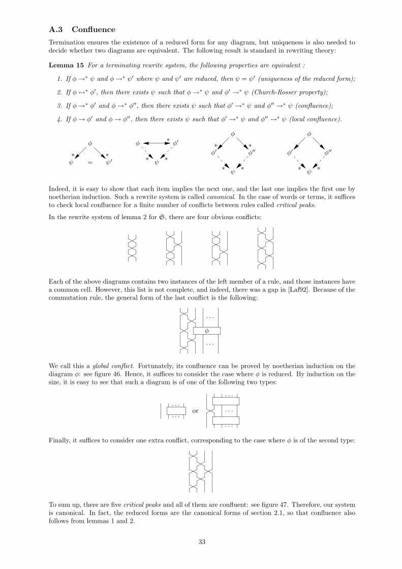
Termination ensures the existence of a reduced form for any diagram, but uniqueness is also needed todecide whether two diagrams are equivalent. The following result is standard in rewriting theory:

Lemma 15 For a terminating rewrite system, the following properties are equivalent :

1. If φ→∗ ψ and φ→∗ ψ′ where ψ and ψ′ are reduced, then ψ = ψ′ (uniqueness of the reduced form);

2. If φ↔∗ φ′, then there exists ψ such that φ→∗ ψ and φ′ →∗ ψ (Church-Rosser property);

3. If φ→∗ φ′ and φ→∗ φ′′, then there exists ψ such that φ′ →∗ ψ and φ′′ →∗ ψ (confluence);

4. If φ→ φ′ and φ→ φ′′, then there exists ψ such that φ′ →∗ ψ and φ′′ →∗ ψ (local confluence).

ψ

φ

ψ′

∗ ∗=

φ′φ

ψ∗ ∗

∗

φ′′φ′

φ

ψ

∗ ∗

∗ ∗

φ

φ′

ψ

φ′′

∗ ∗

Indeed, it is easy to show that each item implies the next one, and the last one implies the first one bynoetherian induction. Such a rewrite system is called canonical. In the case of words or terms, it sufficesto check local confluence for a finite number of conflicts between rules called critical peaks.

In the rewrite system of lemma 2 for S, there are four obvious conflicts:

Each of the above diagrams contains two instances of the left member of a rule, and those instances havea common cell. However, this list is not complete, and indeed, there was a gap in [Laf92]. Because of thecommutation rule, the general form of the last conflict is the following:

φ

· · ·

· · ·

We call this a global conflict. Fortunately, its confluence can be proved by noetherian induction on thediagram φ: see figure 46. Hence, it suffices to consider the case where φ is reduced. By induction on thesize, it is easy to see that such a diagram is of one of the following two types:

· · ·

· · ·· · ·

· · ·

· · ·

or

Finally, it suffices to consider one extra conflict, corresponding to the case where φ is of the second type:

To sum up, there are five critical peaks and all of them are confluent: see figure 47. Therefore, our systemis canonical. In fact, the reduced forms are the canonical forms of section 2.1, so that confluence alsofollows from lemmas 1 and 2.

33

2x+y

x yx y

x+y x 1

Figure 44: Interpretation of the generators

x y

2x+y x+y

x y

yx

x y

3x+2y

x y

2x+y

x y z

3x+y+zx+y

x y z

2x+y+zy

x y z

2x+y+z2x+y

x y z

x+y+z2x+y

x y z

x

2x+y+zx+y

x y z

x

x+y+zx+y

x y z

4x+2y+z

x y z

2x+2y+z4x+2y+z

x y z x y z

2x+2y+z

x y z

x3x+2y+z

x y z

xx+2y+z

x

1x

x

x+1 1

x

x1

x

x+1 x

x

x+2

x

x

x

2x+1

x

x

Figure 45: Termination for F

φ

· · ·

· · ·

φ′

· · ·

· · ·

ψ· · ·

· · ·

φ

· · ·

· · ·

φ′

· · ·

· · ·

φ

· · ·

· · ·

φ′

· · ·

· · ·

∗

∗

Figure 46: Proving the confluence of a global conflict by noetherian induction

34

Figure 47: Confluence of the five critical peaks for S

Figure 48: Confluence of the five critical peaks for M

35

The rewrite system of figure 4 for M is also canonical. In this case, there is no global conflict and thefive critical peaks are confluent: see figure 48. In fact, this system can be identified with the well-knowterm rewrite system for the theory of monoids:

(xy)z → x(yz), 1x→ x, x1 → x.

In the rewrite system of figure 9 for F, there are six global conflicts: see figure 49. Again, it suffices toconsider the case where φ is reduced, and such a diagram is of one of the following four types:

· · ·

· · ·· · ·

· · ·

· · ·

· · ·

· · ·

· · ·

· · ·

or oror

Furthermore, if φ is of the fourth type, we get a reducible conflict. This means that a third rule applies,and the confluence of this conflict can be deduced from the confluence of a smaller conflict: see figure 50.Finally, the global conflicts lead to 6× 3 = 18 critical peaks, and all together, there are 68 critical peaks:see figure 51. The confluence can be checked case by case, but it also follows from section 2.3.

In our examples, the study of critical peaks is not the only way to prove confluence, but the notion isinteresting anyway:

• In [Squ87] and [SOK94], critical peaks are used to compute homological invariants of a monoid.See also [LP91] and [Laf95b] for an introduction. This should be extended to monoidal categories.

• In [Mac71], the critical peaks of figure 48 are used to prove the coherence theorem for (non strict)monoidal categories. Similarly, the canonical system for F can be used to prove the coherencetheorem for symmetric monoidal categories.

A.4 Terms versus diagrams

Any first-order equational theory with n function symbols and r equations corresponds to a presentationby n+ 3 generators and r + 3n+ 7 relations. This presentation consists of:

• one generator α : m → 1 for each function symbol of arity m, and the 3 generators τ : 2 → 2,δ : 1 → 2, and ε : 1 → 0;

• one relation for each equation, 3 relations for each function symbol (see figure 52), and the dual ofthe 7 relations for F.

For instance, the theory of Boolean algebras with 4 function symbols and 10 equations corresponds to thepresentation of theorem 10 for F[2] with 7 generators and 29 relations. This idea comes from [Bur93]. Itis based on Lawvere’s interpretation of algebraic theories by means of Cartesian categories : see [Law63].

There is a similar correspondence for rewrite systems: Any left linear canonical term rewrite system withn function symbols, r rules, and p critical peaks corresponds to a canonical diagram rewrite system withn+3 generators, r+4n+12 rules, and p+4r+n2 +14n+68 critical peaks. In addition to the r originalrules, we have 4 extra rules for each function symbol (see figure 53) and the dual of the 12 rules for F.

Left linearity is a strong restriction: It means that variables occur once in the left member of each rule.For instance, x(y + z) → xy + xz is left linear, but not x + x → 0. Here is the crucial observation: theleft member of such a rule corresponds to a diagram (in fact a tree) with no τ , δ, or ε, and there is nocritical peak between the original rules and those coming from the rules for F. Furthermore, one cancheck that all new global conflicts are reducible. Therefore, it suffices to consider the 5 types of criticalpeaks between the 3 types of rules (see figure 54).

This proliferation of rules and critical peaks is the price to pay for a decomposition of equational reasoninginto more elementary steps. However, we may find canonical systems which are not of the above form:

• If our conjecture about the termination of the rewrite system of figure 28 holds, then we get acanonical system for L(Z2), whereas there is no canonical term rewrite system for the theory ofvector spaces over Z2, simply because the commutativity x + y = y + x cannot be oriented. Thisproblem is usually handled by introducing rewriting modulo associativity and commutativity, butwe claim that our approach is less ad hoc.

• There are useful algebraic structures, such as braids, tangles, and Hopf algebras, which are naturallyexpressed with diagrams, but not with terms. Unfortunately, we have no interesting example ofcanonical system of this kind. For instance, the existence of a finite canonical rewrite system forthe monoidal category of braids is an open question.

36

φ

· · ·

· · ·

φ

· · ·

· · ·

φ

· · ·

· · ·

φ

· · ·

· · ·

φ

· · ·

· · ·

φ

· · ·

· · ·

Figure 49: The six global conflicts for F

∗

Figure 50: Confluence of a reducible conflict

37

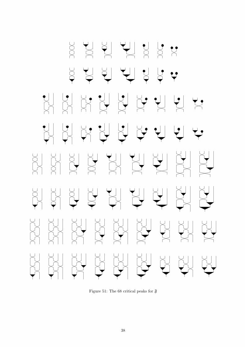
Figure 51: The 68 critical peaks for F

38

= = =

= = =

= = =

Figure 52: Relations for function symbols of arity 0, 1, or 2

Figure 53: Rules for function symbols of arity 0, 1, or 2

r 4n 124r 14n

p n2 68

Figure 54: The 5 types of critical peaks between the 3 types of rules

39

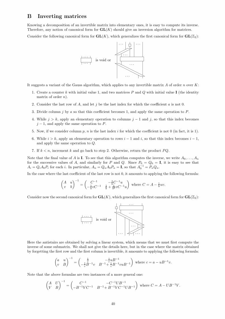
B Inverting matrices

Knowing a decomposition of an invertible matrix into elementary ones, it is easy to compute its inverse.Therefore, any notion of canonical form for GL(K) should give an inversion algorithm for matrices.

Consider the following canonical form for GL(K), which generalizes the first canonical form for GL(Z2):

· · ·

· · ·· · ·

· · ·

· · ·

· · · · · ·

is void or

It suggests a variant of the Gauss algorithm, which applies to any invertible matrix A of order n over K:

1. Create a counter k with initial value 1, and two matrices P and Q with initial value I (the identitymatrix of order n).

2. Consider the last row of A, and let j be the last index for which the coefficient a is not 0.

3. Divide column j by a so that this coefficient becomes 1, and apply the same operation to P .

4. While j > k, apply an elementary operation to columns j − 1 and j, so that this index becomesj − 1, and apply the same operation to P .

5. Now, if we consider column p, n is the last index i for which the coefficient is not 0 (in fact, it is 1).

6. While i > k, apply an elementary operation to rows i− 1 and i, so that this index becomes i− 1,and apply the same operation to Q.

7. If k < n, increment k and go back to step 2. Otherwise, return the product PQ.

Note that the final value of A is I. To see that this algorithm computes the inverse, we write A0, . . . , An

for the successive values of A, and similarly for P and Q. Since P0 = Q0 = I, it is easy to see thatAi = QiA0Pi for each i. In particular, An = QnA0Pn = I, so that A−1

0 = PnQn.

In the case where the last coefficient of the last row is not 0, it amounts to applying the following formula:

(A uv b

)−1

=

(C−1 − 1

bC−1u

− 1bvC−1 1

b+ 1

b2vC−1u

)where C = A− 1

buv.

Consider now the second canonical form for GL(K), which generalizes the first canonical form for GL(Z2):

· · ·

· · ·

· · ·

· · ·

· · ·

· · ·

· · ·

is void or

Here the antistairs are obtained by solving a linear system, which means that we must first compute theinverse of some submatrix. We shall not give the details here, but in the case where the matrix obtainedby forgetting the first row and the first column is invertible, it amounts to applying the following formula:

(a uv B

)−1

=

(1c

− 1cuB−1

− 1cB−1v B−1+ 1

cB−1vuB−1

)where c = a− uB−1v.

Note that the above formulas are two instances of a more general one:

(A UV B

)−1

=

(C−1 −C−1UB−1

−B−1V C−1 B−1+B−1V C−1UB−1

)where C = A− UB−1V .

40