towards a methodology to test uavs in hazardous environments

Towards a Methodology to Test UAVs in Hazardous Environments

Vince Page

School of Engineering

University of Liverpool

Liverpool, United Kingdom

Email: [email protected]

Michael Fisher

Department of Computer Science




Matt Webster

Department of Computer Science




Mike Jump

School of Engineering




ABSTRACT - This paper reports on the early stages of the

development of a methodology to analyse and test autonomous

systems in hazardous environments, with the aim of verifying

both the safe decision-making and resulting actions of the

system. The ultimate goal is to generate safety case evidence that

a designer can provide to a regulator to show that the system to

be used will likely operate safely.

Keywords – UAV; Hazardous Environments; Verification;

Simulation.

I. INTRODUCTION

There is currently a drive in the UK toward using

autonomous systems, and robotic systems in particular, in

extreme or hazardous environments [1]. This paper is

concerned with the Verification and Validation (V&V) of

autonomous systems operating in hazardous (specifically

offshore) environments.

Autonomous systems are systems which decide for

themselves what to do [2]. Typically, these decisions are

made using computer systems, which control the system in

question and perform operations that might otherwise be

performed by a person. For example, an autonomous

Unmanned Aerial Vehicle (UAV) will need to contain a

number of computer systems that can replace a human pilot

operating the UAV using remote control [3].

In this paper, an autonomous system means the following:

A system that is given a goal and restrictions and

fulfils this goal by planning, making decisions and

carrying out actions without direct human

interaction

Robotic systems are good for tasks in hazardous

environments. Typically, robotic systems are used for Dull,

Dirty and/or Dangerous missions, commonly known as the

“three D’s”. Recently however, the need to use robots within

Demanding, Distant and Distributed missions has also been

established. Offshore environments, such as oil platforms and

wind farms, are prime examples of these latter “three D’s”.

In all environments, but in particular for hazardous

environments, autonomous systems must operate safely and

be safe to operate. What is more, this must be demonstrable.

Part of the process to demonstrate this safety case means that

the decisions being made, by the system, the reasons why

they have been made and the actions that result from these

decisions need to be verified for all possible operating

conditions. Furthermore, if a system fails, knowledge

regarding why it fails is required. Thus, the question asked in

this paper is as follows:

How can an autonomous UAV be analysed to

determine the conditions under which it fails and to

indicate why it failed?

This paper uses an example scenario of an UAV

inspecting an offshore asset to demonstrate the development

of tools and techniques that will be used to verify its safe

operation.

The paper is organised as follows. Section II establishes

the challenges of offshore environments for autonomous

systems; how V&V can be used to ensure safety; how a

system needs to be constructed to be verified; how the V&V

outputs can be used to build certification evidence; and how

the methodology presented contributes to this. Section III

presents the methodology to analyse the UAV and provide

explainable failures and Section IV shows the results of its

application and interpretation. Finally, conclusions are drawn

and future work is detailed in Section V.

II. BACKGROUND

A. Offshore Operations

For the purposes of this paper, ‘the offshore environment’

means the environment around energy generation assets, such

as oil rigs and wind turbines.

UAV operations, e.g., remote inspections around oil rigs

and wind turbines, pose many engineering challenges. A

potentially significant source of operational difficulty for

such tasks will be when flying in the disturbed/turbulent air

flow near such structures, as shown in Figure 1. Such

turbulent flow structures make flying in and around the

offshore assets dangerous if the vehicle does not possess

sufficient control authority to maintain its desired position,

leading to a potential collision with the asset or its associated

personnel.

A similar situation exists for ship-borne naval aviation

operations. Helicopters are often operated from landing decks

located at the ship’s stern. The ship’s motion and wind

38Copyright (c) IARIA, 2019. ISBN: 978-1-61208-712-2

ICAS 2019 : The Fifteenth International Conference on Autonomic and Autonomous Systems

mailto:[email protected]




conditions create an area of disturbed air flow in the landing

area. To determine whether a particular ship and helicopter

combination is capable of landing/taking off from the ship

under a given wind condition, flight trials are conducted to

form a Ship Helicopter Operating Limit (SHOL) [4].

Previous work has investigated the replacement of part of the

physical testing required to generate a SHOL with piloted

simulations [4]. The method presented in this paper takes a

similar simulation-based approach for autonomous UAV

system missions.

The scenario considered in this paper is an inspection task

for a UAV on an oil rig leg. This is a sufficiently complex

task to allow the methodology to be rigorously tested. It will

be applied to other, more diverse scenarios at a later date.

B. V&V of Autonomous Systems

Autonomous systems present a significant challenge for

V&V. Many non-autonomous systems are designed to use a

human operator who has overall responsibility for the safe

and reliable operation of the system. Autonomous systems,

on the other hand, cannot assume the presence of the

responsible human, and therefore must manage safe and

reliable operations themselves [5].

Figure 1. A typical offshore UAV operating environment.

V&V for autonomous systems uses many well-

established techniques, as well as some that have been

developed with autonomous systems in mind [5]. At the same

time, experimentation within controlled environments is a

mainstay of engineering best-practice, and is also used for

autonomous systems. However, due to the significant

challenges and added complexity of autonomous systems,

experimentation can be expensive and dangerous. Therefore,

high-fidelity simulation is often used as a separate V&V

technique [6]. High-fidelity simulation involves

incorporating accurate physical models of a system within a

realistic synthetic environment. Trials within high-fidelity

simulation provide a safer and potentially cheaper means to

test than physical experiments. Of course, this comes at the

cost of needing to understand the limitations of the models

being used. The models of the system and the environment

used within simulation must themselves be verified and

validated [7].

Figure 2. System Architecture of an Autonomous UAV with the separation

of the component using layers which then indicates the verification method to be applied to each

A V&V technique commonly used for autonomous

systems is formal verification, an application of Formal

Methods [8]. Formal verification works by building abstract

mathematical models of the system in question, and then

exhaustively analysing the models using software to

determine whether or not particular requirements hold.

Formal verification is particularly useful for finite state

systems, and has therefore found a natural application in the

verification and validation of autonomous software.

There are, of course, many other V&V techniques not

listed above, including hardware-in-loop testing [9], real-

world operations and end-user validation [10], that are also

used for V&V of autonomous systems.

C. Systems Architecture for V&V

To be able to apply V&V to a whole system, it needs to

be constructed in a certain way. This is mostly due to the

models used to describe a sub-system. In Figure 2, the

systems architecture of an autonomous system that is to fly

UAVs around oil rigs is shown. There are two important

features in this architecture: the layers and the intra-layer

separation of subsystems.

The layering is to group sub-systems, similar in

construction rather than role or output. The calculation layer

can be thought of as any task that reasons about the world in

a non-abstract way, such as a route or mission planner. The

decision layer is for those systems that make decisions based

on information provided by the interaction and calculation

layers. The interaction layer is the-low level autonomous

tasks that translates plans and decisions into actions. The

environment layer is the actual hardware that physically

carries out the desired actions.

On the right of Figure 2, the verification methods are

aligned with the components that they are best suited to

testing. Formal methods are well suited to analysing and

verifying decision making, but the abstraction required to

apply them to planners or continuous controllers makes them

less so for these elements. Simulation-based testing allows



many permutations of the systems goals, initial conditions

and even internal parameters, to be tested; thus allowing the

actions of the systems to be rigorously tested. The physical

testing of the system then checks the results of the formal

methods and simulations against reality and will determine

the validity of the abstractions and assumptions required to

build them.

In short, with the system constructed in such a way, the

following questions can be answered:

Formal Methods - Has the safe decision been made?

Simulation Based Testing - Did it result in safe actions?

Physical Testing - How well do these answers match

reality?

D. Evidence for Safe Operations

For an autonomous system to be used in a real-world

environment, its safe operation needs to be agreed with the

regulator. In the UK, there is no standard method for

assessing whether or not autonomous UAV operations are

safe. Each request for operation is reviewed on a case-by-case

basis using a submitted safety case/risk assessment for the

planned operation.

V&V techniques can be used to generate evidence to

prove that a system will operate safely and reliably. This

paper proposes that formal methods and simulation based

stress testing can be included to add strength to the safety

case.

For the scenario considered in this paper, the operating

envelope of the system, when being used in certain conditions

is the addition to the safety case. An example of this is shown

in Figure 3. This example is intentionally similar to that of a

SHOL. The aim of simulation-based verification is to

generate this operating envelope. The dotted lines represent

the boundary between safe and unsafe operations.

As an example, for a UAV doing inspections of the legs

of an oil rig, there will exist a set of wind speeds and

directions under which the UAV is no longer able to operate.

The operator of the UAV, oil rig and regulators will need to

know the safe wind speed and direction operating envelope

before any task can proceed.

Figure 3. Illustration of the safety case evidence aimed for when using the

methodology.

In addition, for this situation the variables that affect the

safe operation of the UAV are not restricted to just the wind

speed and direction. They could include, but are not limited

to, the following:

• Initial position and goal

• Geometry of environment

• UAV performance capability

• Actuator/sensor performance/degradation

• Other environmental conditions e.g. ambient light,

sea state etc.

This means that the real operating envelope will be a

multi-dimensional surface.

It is important to note here that such a surface can not only

be used as safety-case evidence, but also as a run-time safety

monitor. The analogy is that the boundary is the equivalent of

the prior experience of the human pilot, where they intuitively

know what actions and decisions are a good idea or not. This

can then be used, while the system is in operation, to inform

the autonomous system of when it is feasible to carry out a

plan or not; or as a monitor to tell the system that, as the

environment changes, planned actions or current states (such

as where it is) are no longer safe.

E. Understanding the System’s Failure

If a system is tested under one set of conditions and is

found to successfully complete the task assigned to it safely,

this is good. If under slightly different conditions, the system

fails to complete it safely, this is also good. This now informs

both the user and the system itself, when it should and should

not carry out particular actions. This is the essence of the

operating envelope shown in Figure 3. However, this does not

inform the user, or regulator, why the system failed.

It is far more useful to be able to say under what

conditions a system can or cannot work and to also to be able

to say why. This both directs any effort to redesign or

improve the system, as the designer now knows which system

to focus on; and it provides the regulator with a more concrete

answer as to why it behaves in the way it does.

As an example, suppose there are measures of failure for

an actuator, controller, guidance, and navigation of a UAV

(more on this in Section III). After a simulation of a task, at a

number of wind speeds and directions, these failure measures

are then applied to the response, a possible result could be as

shown in Figure 4 (a). Outside of this boundary, the system

failed its task, while inside it succeeded. The aggregate of

these failure results in Figure 4 (b).

This boundary is now the operating envelope of the

system. However, by splitting the failure of the system into

separate components, the colours shown can be added. This

then indicates that the actuator, at least in this example, was

the most likely cause of the system to fail its task.

III. METHODS

This section describes the cost functions and

methodology used to apply V&V ideas to an autonomous

systems.



A. Cost functions for each component

Four continuous autonomy components are considered.

The responsibility of each component, what its job is,

determines the definition of the cost function. The

responsibilities of each component are as follows:

Actuator: To create the required output while leaving a

margin of error as a contingency.

Controller: To force the current states to follow the

commanded states as closely as possible, while

maintaining system stability.

Guidance: To cause the system to follow the desired

path to within a desired separation distance.

Navigation: To generate a path between the start and

goal, while avoiding collisions with objects.

The cost function defining the actuator’s performance is

shown in (1) and illustrated in Figure 5.

𝐴𝑓 =1

𝑛𝑎∑

1

𝑡𝑚∫

√(𝐴𝑖 − .5)2

. 5 − 𝑀𝑎𝑟𝑑𝑡

𝑡𝑚

0

𝑖=𝑛𝑎

1

(1)

Where 𝑛𝑎 is the number of actuators, 𝑡𝑚 is the maximum

simulation time, 𝐴𝑖 the actuator output at time 𝑡, 𝑀𝑎𝑟 the

specified margin of error, and 𝑑𝑡 the time step of the

simulation.

Here, the zero point for the actuator is 50%. The function

is, in essence, a time average of the deviation from the neutral

point normalised by the margin of error. The performance of

all the actuators is averaged over time and over the number

of actuators.

This function aims to create a single measure for all the

actuators over the time period of operation between 0 and 1.

The cost function gives a gradual increase in the failure. If an

actuator reaches either 100% or 0%, this results in the failure

of the system being set to 1. This can be considered a critical

failure, as would a collision, since the system would very

likely become unsafe.

The controller’s performance is defined in (2) and shown

in Figure 6.

𝐶𝑓 =1

𝑛𝑠∑

1

𝑡𝑚∫

√(𝑅𝑖 − 𝑢𝑖)2

𝐷𝑖𝑓𝑖𝑑𝑡

𝑡𝑚

0

𝑖=𝑛𝑠

𝑖=0

(2)

Where 𝑛𝑠 is the number of controlled states, 𝑅𝑖 is the

command reference, 𝑢𝑖 the measured state of the system, and

𝐷𝑖𝑓𝑖 the specified max difference between the actual and

reference values.

It is essentially the same as the cost function used in

Linear Quadratic Regulator controllers. The difference

between the reference and controlled state is normalised by a

desired maximum distance. It is then averaged over both time

and the number of controlled states. A discontinuity exists

when the system becomes unstable.

The guidance performance is defined by both in (3) and

Figure 7.

𝐺𝑓 =1

𝑡𝑚∫

√(𝛿𝑥 + 𝛿𝑦 + 𝛿𝑧)2

𝐷𝑖𝑣𝑑𝑡

𝑡𝑚

0

(3)

Where 𝛿𝑥, 𝛿𝑦, and 𝛿𝑧 are the orthogonal difference

between the actual position and the desired path and 𝐷𝑖𝑣 is

the specified maximum deviation from the path.

It is the length of the vector perpendicular to the nearest

point on the desired path from the system’s current location.

It is then normalised by the desired maximum deviation from

the path. A discontinuity does not explicitly exist with this

function, however the discontinuities are handled by the

mission manager’s performance, see Criteria Analysis

section later.

The navigation’s performance is defined by (4) and by

Figure 8.

𝑁𝑓 =1

𝑡𝑚∫

𝑃𝑟𝑜𝑥

𝑃

𝑡𝑚

0

𝑑𝑡 (4)

Where 𝑃𝑛 is the planned proximity at the point on the path

perpendicular to the current position, 𝑃 the proximity to the

nearest object, and 𝑃𝑟𝑜𝑥 is the specified maximum proximity

to an object.

Figure 4. Illustration of how the subsystems can be combined and therefore allow the explanation of why a system failed to operate safely



Figure 5. Definition of cost function for the analysis of the actuator’s

performance

Figure 6. Definition of cost function for the analysis of the controller's

performance

Figure 7. Definition of the cost function for the analysis of the guidance

performance

Figure 8. Definition of the cost function for the analysis of the navigation

performance

B. Simulation Environment

A simple simulation environment of a helicopter moving

around the legs of an oil rig is used to generate the data

required to test the above cost functions, see Figure 9.

It consists of a series of linearized state space flight

dynamics models identified from a non-linear simulation

model. The models are then scheduled based on the forward

flight speed of the UAV, to account for the changing

dynamics.

To control the helicopter a PI controller [11] is gain

scheduled and a waypoint following with cross tracking error

is used as the guidance method [12]. A simple A* route

finding algorithms is used for the navigation [13], where a

simple hazard model is used to allow the planner to plan a

route around the wakes of the oil rig legs.

A sample data set is taken from the simulation

environment and presented in the next section. The cost

functions are then applied to the output of the simulator.

Figure 9. Systems diagram for the simulator

IV. RESULTS

When testing and analysing an autonomous system’s

performance, a designer may be presented with the output

shown in Figure 10 to Figure 12. From this the designer

would be able to determine whether the UAV was able to

carry out the task assigned to it. In this case, simply move

from bottom left to the right of the top right leg.

However, some of the routes come very close to the legs,

to the point where a collision is very likely. This is also for

only a single set of conditions, but can only be interpreted

visually. If the conditions change, will the UAV be able to

still carry out the task? How does this compare to other UAVs

or settings/weightings within the autonomous components of

the UAV?

A closer inspection of the least risky plan’s response of

the UAV can be seen in Figure 13, Figure 14, and Figure 15.

From this, it can be determined that the control input is not

exceeded, the body velocities follow the reference values and

the UAV follows the desired path reasonably well. However,

again this does not allow an easy comparison to other UAVs

or settings. The interpretation is also abstract and not

quantified.

Further detail can be determined from Figure 16 and

Figure 17, where how well the UAV followed the planned

path and how well the plan enabled the UAV to avoid

collisions with its surroundings is shown. The actuator cost

function can be applied to the results in Figure 13, the

controller function to Figure 14, the guidance function to

Figure 16 and the navigation function to Figure 17.



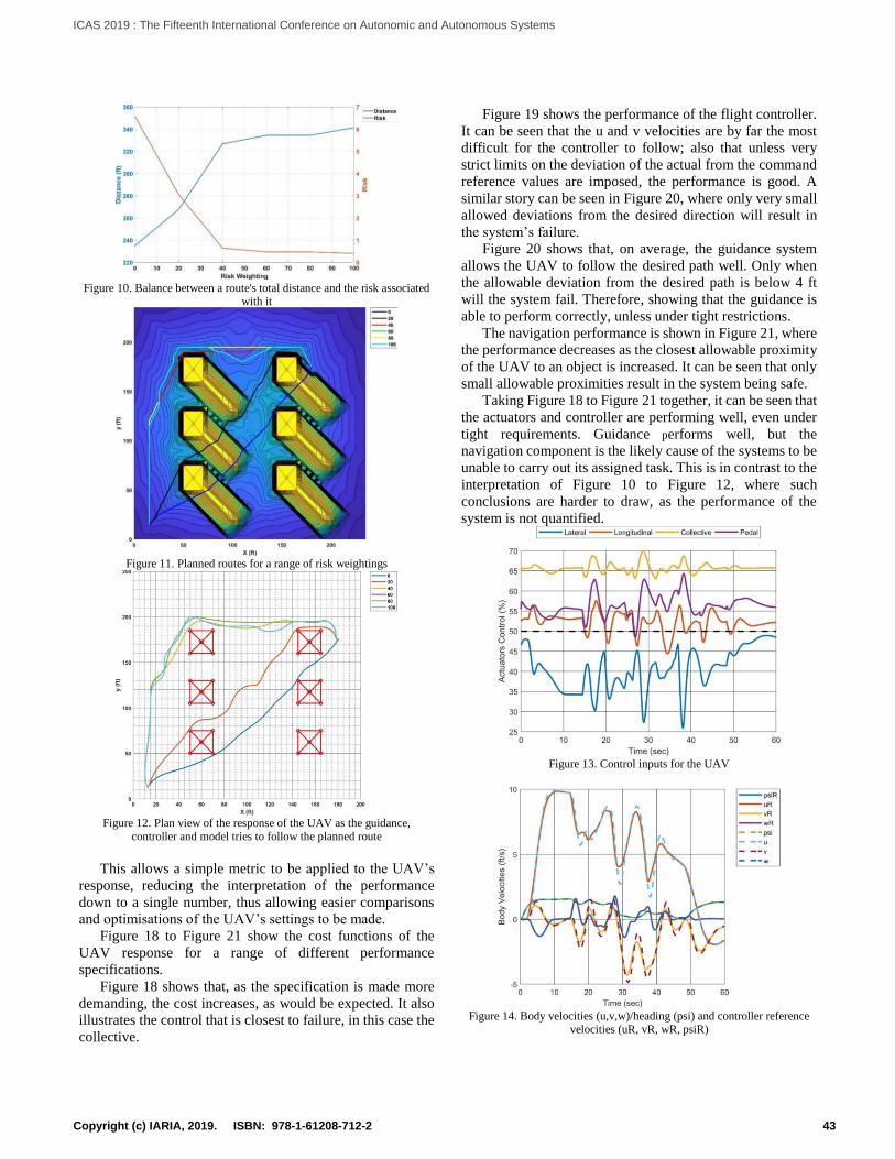
Figure 10. Balance between a route's total distance and the risk associated

with it

Figure 11. Planned routes for a range of risk weightings

Figure 12. Plan view of the response of the UAV as the guidance,

controller and model tries to follow the planned route

This allows a simple metric to be applied to the UAV’s

response, reducing the interpretation of the performance

down to a single number, thus allowing easier comparisons

and optimisations of the UAV’s settings to be made.

Figure 18 to Figure 21 show the cost functions of the

UAV response for a range of different performance

specifications.

Figure 18 shows that, as the specification is made more

demanding, the cost increases, as would be expected. It also

illustrates the control that is closest to failure, in this case the

collective.

Figure 19 shows the performance of the flight controller.

It can be seen that the u and v velocities are by far the most

difficult for the controller to follow; also that unless very

strict limits on the deviation of the actual from the command

reference values are imposed, the performance is good. A

similar story can be seen in Figure 20, where only very small

allowed deviations from the desired direction will result in

the system’s failure.

Figure 20 shows that, on average, the guidance system

allows the UAV to follow the desired path well. Only when

the allowable deviation from the desired path is below 4 ft

will the system fail. Therefore, showing that the guidance is

able to perform correctly, unless under tight restrictions.

The navigation performance is shown in Figure 21, where

the performance decreases as the closest allowable proximity

of the UAV to an object is increased. It can be seen that only

small allowable proximities result in the system being safe.

Taking Figure 18 to Figure 21 together, it can be seen that

the actuators and controller are performing well, even under

tight requirements. Guidance performs well, but the

navigation component is the likely cause of the systems to be

unable to carry out its assigned task. This is in contrast to the

interpretation of Figure 10 to Figure 12, where such

conclusions are harder to draw, as the performance of the

system is not quantified.

Figure 13. Control inputs for the UAV

Figure 14. Body velocities (u,v,w)/heading (psi) and controller reference

velocities (uR, vR, wR, psiR)



Figure 15. UAV (x, y, z) and reference (xref, yref, zref) positions

Figure 16. Plan view of the UAVs response when following the least risky

planned route. Solid line = planned route. Dashed line = path taken

Figure 17. Actual and planned proximity to the nearest object at a point in

time in the UAV's response

Figure 18. Performance metric for the actuator when applied to the UAV's

response for a range of specifications

Figure 19. Controller performance for the body velocities for a range of

specifications

Figure 20. Controller performance for the direction command reference



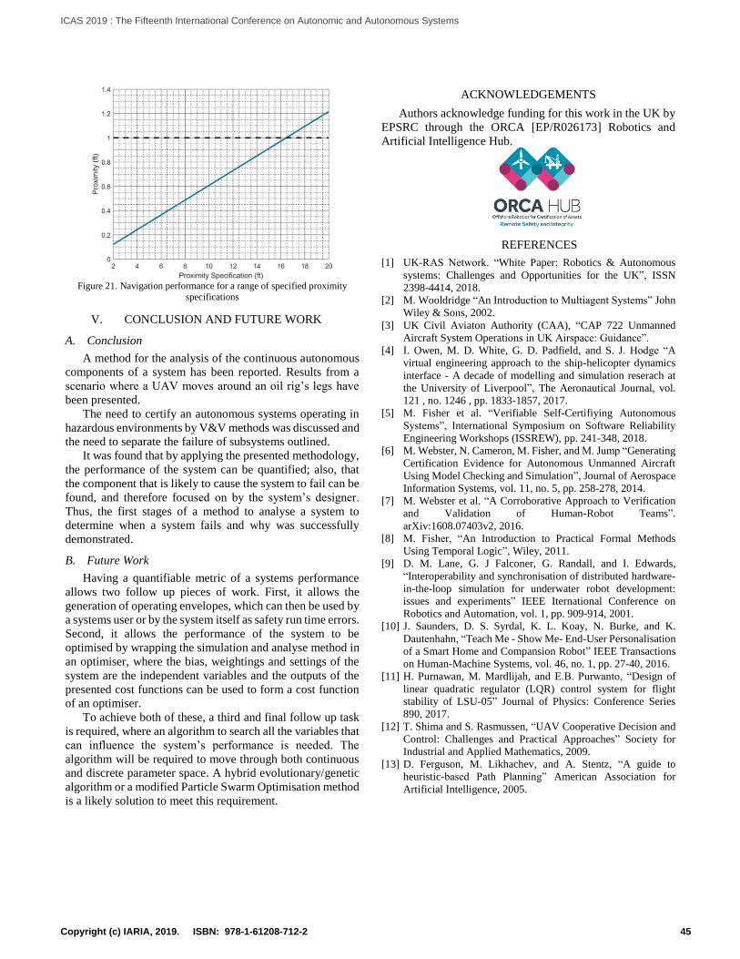
Figure 21. Navigation performance for a range of specified proximity

specifications

V. CONCLUSION AND FUTURE WORK

A. Conclusion

A method for the analysis of the continuous autonomous

components of a system has been reported. Results from a

scenario where a UAV moves around an oil rig’s legs have

been presented.

The need to certify an autonomous systems operating in

hazardous environments by V&V methods was discussed and

the need to separate the failure of subsystems outlined.

It was found that by applying the presented methodology,

the performance of the system can be quantified; also, that

the component that is likely to cause the system to fail can be

found, and therefore focused on by the system’s designer.

Thus, the first stages of a method to analyse a system to

determine when a system fails and why was successfully

demonstrated.

B. Future Work

Having a quantifiable metric of a systems performance

allows two follow up pieces of work. First, it allows the

generation of operating envelopes, which can then be used by

a systems user or by the system itself as safety run time errors.

Second, it allows the performance of the system to be

optimised by wrapping the simulation and analyse method in

an optimiser, where the bias, weightings and settings of the

system are the independent variables and the outputs of the

presented cost functions can be used to form a cost function

of an optimiser.

To achieve both of these, a third and final follow up task

is required, where an algorithm to search all the variables that

can influence the system’s performance is needed. The

algorithm will be required to move through both continuous

and discrete parameter space. A hybrid evolutionary/genetic

algorithm or a modified Particle Swarm Optimisation method

is a likely solution to meet this requirement.

ACKNOWLEDGEMENTS

Authors acknowledge funding for this work in the UK by

EPSRC through the ORCA [EP/R026173] Robotics and

Artificial Intelligence Hub.

REFERENCES

[1] UK-RAS Network. “White Paper: Robotics & Autonomous

systems: Challenges and Opportunities for the UK”, ISSN

2398-4414, 2018. [2] M. Wooldridge “An Introduction to Multiagent Systems” John

Wiley & Sons, 2002.

[3] UK Civil Aviaton Authority (CAA), “CAP 722 Unmanned

Aircraft System Operations in UK Airspace: Guidance”.

[4] I. Owen, M. D. White, G. D. Padfield, and S. J. Hodge “A

virtual engineering approach to the ship-helicopter dynamics

interface - A decade of modelling and simulation reserach at

the University of Liverpool”, The Aeronautical Journal, vol.

121 , no. 1246 , pp. 1833-1857, 2017.

[5] M. Fisher et al. “Verifiable Self-Certifiying Autonomous

Systems”, International Symposium on Software Reliability

Engineering Workshops (ISSREW), pp. 241-348, 2018.

[6] M. Webster, N. Cameron, M. Fisher, and M. Jump “Generating

Certification Evidence for Autonomous Unmanned Aircraft

Using Model Checking and Simulation”, Journal of Aerospace

Information Systems, vol. 11, no. 5, pp. 258-278, 2014.

[7] M. Webster et al. “A Corroborative Approach to Verification

and Validation of Human-Robot Teams”.

arXiv:1608.07403v2, 2016.

[8] M. Fisher, “An Introduction to Practical Formal Methods

Using Temporal Logic”, Wiley, 2011.

[9] D. M. Lane, G. J Falconer, G. Randall, and I. Edwards,

“Interoperability and synchronisation of distributed hardware-

in-the-loop simulation for underwater robot development:

issues and experiments” IEEE Iternational Conference on

Robotics and Automation, vol. 1, pp. 909-914, 2001.

[10] J. Saunders, D. S. Syrdal, K. L. Koay, N. Burke, and K.

Dautenhahn, “Teach Me - Show Me- End-User Personalisation

of a Smart Home and Compansion Robot” IEEE Transactions

on Human-Machine Systems, vol. 46, no. 1, pp. 27-40, 2016.

[11] H. Purnawan, M. Mardlijah, and E.B. Purwanto, “Design of

linear quadratic regulator (LQR) control system for flight

stability of LSU-05” Journal of Physics: Conference Series

890, 2017.

[12] T. Shima and S. Rasmussen, “UAV Cooperative Decision and

Control: Challenges and Practical Approaches” Society for

Industrial and Applied Mathematics, 2009.

[13] D. Ferguson, M. Likhachev, and A. Stentz, “A guide to

heuristic-based Path Planning” American Association for

Artificial Intelligence, 2005.



towards a methodology to test uavs in hazardous environments

Documents