Toward improving the representation of the

water cycle at High Northern Latitudes

W. A. Lahoza, T. M. Svendbya, A. Griesfellera, J. Kristiansenb

a NILU, Kjeller, Norwayb Met Norway, Oslo, Norway

wal@nilu.no

Outline

Introduction

• Background: rapid warming at Northern Latitudes

• Difficulties of measuring soil moisture at Northern High Latitudes

• Data sources for Northern High Latitudes: satellite/in situ

Data – in situ/satellite (different characteristics)

Comparison in situ and satellite soil moisture – Norway

• Time-series: 2009-2014

• Extreme events: droughts/floods

Summary and future work (e.g., data assimilation)

• Example of early results from data assimilation

Introduction

Rapid warming Northern Latitude regions in recent decades -> lengthening of growing season, greater photosynthetic activity & enhanced carbon sequestration by ecosystem

(Barichivich et al. 2014 & references therein)

Changes likely to intensify summer droughts, tree mortality & wildfires

Potential major climate change feedback is release of carbon-bearing compounds from soil thawing - e.g., methane, carbon dioxide

(Woods Hole Research Center, Holmes et al., 2015, Policy Brief)

………. =Mean summer T anomalywrt 1961-1990

Proxy regionalsummer droughts

1988

1997

Example of changes at northern high latitudes:

PDSI = Palmer Drought Severity Index (sc self-calibrating)PET = potential evapotranspiration: red/blue (with/without interannual PET changes)

Al Yaari et al. 2014

Surface soil moisture- SSM

• AMSR-E product

• SMOS L3 product

Wrt to reference:

• DAS2 ECMWFSSM from Land DA

(ASCAT SM + 2m T/RH)

03/2010 - 09/2011

AMSR-E SMOSProblems with satellitedata at N. high latitudes

High RMSD

+ve/-ve

High bias

Low corr

Important to have information on land surface (soil moisture & temperature) at high northern latitude regions

Availability of soil moisture measurements from satellites -> opportunity to address issues associated with climate change: assessing multi-decadal links between increasing temperatures, snow cover, soil moisture variability & vegetation dynamics (Barichivich et al. 2014 & references therein)

Relatively poor information on water cycle parameters for biomes at northern high latitudes (boreal humid – Scandinavia) make it important efforts made on improving representation of water cycle at these latitudes (Al Yaari et al. 2014; van der Schalie 2015)

Why soil moisture retrieval difficult over Norway

SMOS, 2011-06-11

soil moisture (m3/m3)

forest; rocks;

moderate topography;

strong topography;

wet snow; open water

fraction > 10%

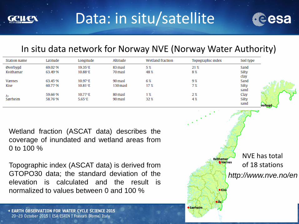
Data: in situ/satellite

In situ data network for Norway NVE (Norway Water Authority))

Wetland fraction (ASCAT data) describes the

coverage of inundated and wetland areas from

0 to 100 %

Topographic index (ASCAT data) is derived from

GTOPO30 data; the standard deviation of the

elevation is calculated and the result is

normalized to values between 0 and 100 %

NVE has totalof 18 stations

http://www.nve.no/en

Time-series of satellites (1978- present)

ESA CCI soil moisture website: http://www.esa-soilmoisture-cci.org/

Satellite-derived soil moisture

ASCAT (Advanced SCATterometer):•Launched October 2006•Active scatterometer•C-Band, 5.255 GHz : 1 cm depth•Descending orbit 9:30, ascending orbit 21:30

SMOS (Soil Moisture and Ocean Salinity):•Launched November 2009•Passive radiometer•L-Band, 1.4 GHz : 5 cm depth•Ascending orbit 06:00, descending orbit 18:00

Co-location criterion in situ/satellite:Make comparison if in situ data falls within lat-long grid associated with orbit swath:

0.3ox0.3o – SMOS 0.1ox0.1o – ASCAT (latitude dependent)

NVE in situ data

Data provided by NVE (unofficial product)

Six NVE stations: Ås, Kise, Øverbygd, Særheim, Værnes and Kvithamar. For Værnes, soil moisture not measured in 2013 and 2014. For Kvithamar no data exist in 2009 and after 2012

SMOS: no satellite data exist in grids covering Ås, Øverbygd & Særheim. For Særheim, satellite overpass data from a neighbouring grid used, but these data less representative

ASCAT: no overpass data retrieved for Kvithamar

Griesfeller et al. (2015) considered period 2009-2011 for AMSRE-/NVE comparison

Satellite data used

ASCAT: Product version WARP 5.5, Release 2.2. Data downloaded from H-SAF FTP server (ftp://ftphsaf.meteoam.it), 11-08-2015. H-SAF website http://hsaf.meteoam.it

SMOS: Soil Moisture (SM) products between 12-01-2010 and 31-12-2013 (tagged RE02). Operational data after 2021-12-2013 (tagged OPER). Downloaded from http://www.catds.fr/sipad/login.do, 24-08-2015

Note: SMOS data version not uniform 2010-2014, focus on 2010-2013. Data from 2014 are not reprocessed

Statistics based on filtering & normalization method used for 2009-2011 analysis (Griesfeller et al., 2015)

Data preparation

ASCAT soil moisture data provided as degree of saturation from 0 % (dry) to 100 % (saturated); for comparison with volumetric in situ data convert the ASCAT data to volumetric soil moisture values (m3m-3)

Exponential filter first described by Wagner et al. (1999); this filter is used to estimate root-zone soil moisture (specified as SWI, m3m−3)

- Can use land data assimilation to estimate root zone soil moisture

ASCAT and SMOS data are normalized using the mean and standard deviation of in situ data (Brocca et al. 2013)

– other approaches possible (e.g., CDF-matching)

Comparison

Results: Figures/1

Ås

Øverbygd

Year

Figures/2

Værnes

Kvithamar

Year

Figures/3

Kise

Year 2013

Comparison: Summary Tables

SMOSAsc «better»

ASCATDes «better»

Extreme events for Norway

• Floods – see image:

• May 2013 – Southern & Eastern Norway (Kise & Ås NVE stations)

• Sep-Oct 2014 – Western Norway (No NVE stations)

• May 2015 – Eastern Norway (Kise NVE station)

• Droughts (Southern & Eastern Norway) – see maps:

• Jan-Feb 2014 – extremely light precipitation

• Mar 2014 – positive temperature anomaly

• Kise: only 1st half Jan/2nd half Feb

• Øverbygd: March

• Ås:Throughout

24 May 2013 – Eastern Norway

Source: Dagbladet

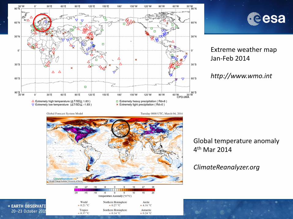
Extreme weather mapJan-Feb 2014

http://www.wmo.int

Global temperature anomaly4th Mar 2014

ClimateReanalyzer.org

Results extreme events – Figures

NVE

ASCAT &SMOS

Year

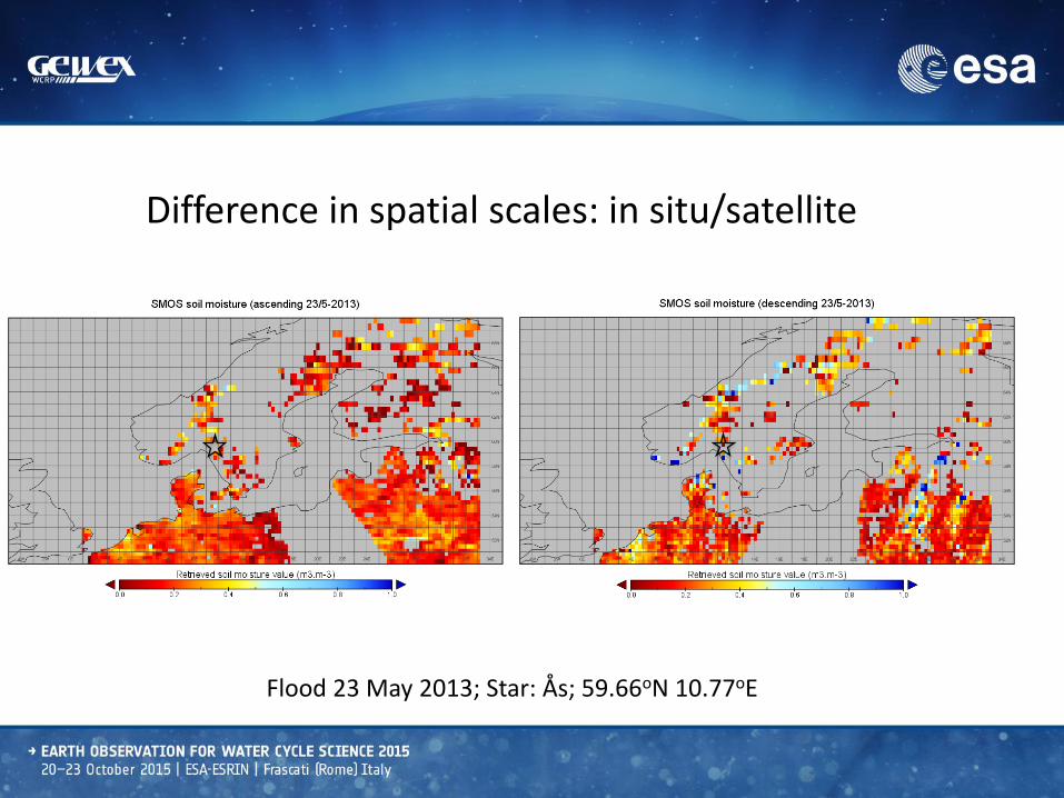
Flood 23 May 2013; Star: Ås; 59.66oN 10.77oE

Difference in spatial scales: in situ/satellite

Summary

Norway one of most challenging regions for measurements of soil moisture

First time soil moisture data from satellite platforms evaluated over Norway

- extends the work in Griesfeller et al., 2015

Averaged correlations of satellite/in situ data over Norway relatively high for some stations (particularly for ASCAT) – this result is not expected

Capture of extreme events over Norway (in situ/satellite data)

Satellite soil moisture information over Norway is useful!

SMOS: ascending generally better than descending orbit

ASCAT: descending generally better than ascending orbit

ASCAT generally performs better than SMOS

Future work Extend collaboration with NVE – improved data use, error characterization

Land data assimilation of soil moisture, with focus on flood/drought events:

(i) benefit for forecasts of hydrological cycle (NILU); and (ii) benefit for NWP

forecasts (Met Norway) – preliminary land data assimilation of ASCAT,

SMOS and AMSR-E data for 1-month in 2011 (July)

•Land DA statistics (e.g., SMOS): consistent with 0.04 m3m-3 error for SMOS

Example (EnKF):test vs independentdata over Europee.g., Urgons, FranceSMOSMANIA

Replicate for Norway

Extra slides

Tables/1

Tables/2

Data assimilation study – Jul 2011

Satellite information – unscaled, July – top: mean; bottom: std

ASCAT converted to m3m-3 using % -> (0,1)Assumes max/min values are 100%, 0% (approx.)

SMOS drierASCAT more variable

Satellite data

Model – SURFEX (Le Moigne 2012):July – top: mean; bottom: std

Scale satellite data to model data –account for bias & variability:

Linear re-scaling (Brocca et al., 2013):

SAT : satellite; OBS : model

Satellite data: same mean & std as model over July 2011

Focus on satellite anomaliesLook at selected days & time series

N.B. CDF-matching inappropriatelength of time series is too short – future work

Model data

Satellite information 5 July – top: unscaled; bottom: scaled

Scaling: dries AMSR-E, ASCAT, moistens SMOSWhite areas: either no data, or data off-scale

Scaling data

Combine obs & model information + errors Lahoz & De Lannoy, Surv. Geophys., 2014

Focus on July 2011 – European domain – short period so care with stats

EnKF (variants) – use ensemble square root EnKF (Sakov and Oke, 2008)

• Model spin-up (1 month)• Model forcing from WRF (NCAR FNL data) – check representation of precipitation• Five ensemble members (can choose other sizes)• Perturbation of superficial & mean volumetric water content -precipitation forcing available but not used; mean of ensemble = 0• Scale observations to model (linear re-scaling; other options)• Test observational errors (chi-square approach)• Test system using self-consistency (O-F vs O-A differences)• Test results against independent data (ISMN in situ data) – also ESA CCI data

Land DA results are preliminary & illustrative

Data assimilation

N = no. of obs (July); F = forecast; A = analysis:

Chi-sq(A) = (1/N) * SUM[(O-A)^2 / R] Chi-sq(F) = (1/N) * SUM[(O-F)^2 / R]

1. O-A differences should be smaller than O-F differences – self-consistency test; passed

2. Chi-sq values should be close to 1 – observational error information

SMOS (N=547431)

– YERROBS=0.1 - Chi-sq(A) = 8.88

– YERROBS=0.1 - Chi-sq(F) =64.45

– YERROBS=0.3 - Chi-sq(A) = 2.86

– YERROBS=0.3 - Chi-sq(F) = 6.79

– YERROBS=0.6 - Chi-sq(A) = 1.11

– YERROBS=0.6 - Chi-sq(F) = 1.69

• AMSR-E (N=949842)

– YERROBS=0.3 - Chi-sq(A) = 2.71

– YERROBS=0.3 - Chi-sq(F) = 6.38

• ASCAT (N=1007729)

– YERROBS=0.3 - Chi-sq(A) = 2.72

– YERROBS=0.3 - Chi-sq(F) = 6.45

SURFEX code - observational error defined asR = (YERROBS*COFSWI)^2

YERROBS, parameter set in input file: typically use 0.3

COFSWI=(Wfc-Wwilt) typical range 0.06- 0.09

Error associated with SMOS anomalies is in range0.036 – 0.054 m3m-3 when YERROBS=0.6

Consistent with a SMOS error of 0.04 m3m-3

Kerr et al., 2010

Observations: self-consistency tests; evaluation of errorsChi square approach applied to corrected satellite data

Tests

July, SMOS, Differences: analyses – modelLeft: unscaled SMOS; Right: scaled SMOS

Regions of larger impact in unscaled version replicated in scaled version - e.g., France/Germany/England

SMOSMANIA - Urgons 43.54N, 0.43W 145 masl

SMOSMANIA - France

Test v independent dataTime series: analyses vs ISMN data – July 2011Thanks Morgan Kjølerbakken