toward an efficient algorithm for the single source shortest path problem on gpus

Toward An Efficient Algorithm for the Single Source Shortest Path Problem on GPUs

Thang M. Le David R. Cheriton School of

Computer Science University of Waterloo [email protected]

Abstract Accelerating graph algorithms on GPUs is a fairly new research area. The topic was first introduced in [3] by Harish and

Narayanan in 2007. Since then, there have been numerous studies on different aspects of graphs on GPUs. Some great work has

been done on graph traversal [4] [5]. Nevertheless, there has not much focus on designing an efficient algorithm for the single

source shortest path (SSSP) problem on GPUs. This report summarizes our study which contains various algorithms and their

performance results for the SSSP problem on GPUs.

1. Introduction

Finding SSSP is a classical problem in graph theory. Dijkstra’s algorithm and Bellman Ford algorithm are the two well-known

solutions for this problem. While Dijkstra’s algorithm is focusing on work efficiency which forces it to make the greedy step at each iteration by choosing the vertex having the smallest distance, Bellman Ford algorithm is exploring all possible vertices in an

effort to reduce a number of iterations at the cost of efficiency. The difference of the two approaches is similar to the difference

of the single instruction single data (SISD) model and the single instruction multiple data (SIMD) model proposed in [1]. Since

GPUs architecture embraces single instruction multiple thread (SIMT), a variant of SIMD, Bellman Ford algorithm is favorable

on GPUs. Although Bellman Ford algorithm provides a great advantage by exploring multiple vertices at a time, our experiments reveal its performance on GPUs is poor due to its inefficient approach. The main reason is the GPU global memory has a high

latency access. As a result, the advantage of parallelism does not compensate for the cost of memory accesses.

In our report, all of the experiments performed on the GPU are compared with our implementation of Dijkstra’s algorithm using

priority queue on the CPU. We chose binary heap data structure to efficiently maintain the priority queue. Based on this

implementation, the runtime complexity of Dijkstra’s algorithm is where is the number of edges, is the

number of vertices. On sparse graphs, this runtime complexity becomes . This is a much faster version compared with

the implementation of Dijkstra’s algorithm using ordinary array or linked list which is . For each design and

implementation, we will discuss advantages and drawbacks. All of the performance results were performed on Tesla server

equipped with two CPUs Intel Xeon DB Quad Core E5620 2.4 Ghz, 4 NVIDIA Tesla C2050, 24GB 1333MHz ECC DDR3 of memory and two 600GB Segate Cheetah 15000rpm 16MB Cache with a RAID controller.

2. Verification

Running on a massive parallel hardware such as GPUs gave us a lot of challenges. Not only did our algorithms face a high risk of racing condition, they exhibited the threat of working on stale data due the inconsistency between cache and memory in CUDA.

In fact, cache coherency issue was the biggest challenge we experienced when working with NVIDIA GPU processor. Because

of all of these risks, we put a lot of effort in simplifying our designs and implementations as much as p ossible. This helped us in

verifying the correctness and troubleshooting effort. In term of testing, we first made sure having a correct Dijkstra’s

implementation. We then relied on this to ensure the GPU algorithms produce the same result as of the Dijkstra implementation. Not only did we compare shortest distances in both results, we used shortest path to recalculate the corresponding shortest

distance and compare it with the shortest distance computed by the algorithm. Although we can reason about the correctness of

our algorithms, we cannot guarantee our implementations are free from bugs. In the end, Dijkstra used to say “Testing shows the

presence, not the absence of bugs”. We welcome you to report any unexpected results to us or send us your comments for

improvements.

3. Usage Usage:

dijkstra.exe [options] [graph_file]

Options: -m <mode> : set the exxecution mode (default 0)

0 -- verification (runs GPU & CPU code and compares)

1 -- GPU only

2 -- CPU only -n <num_sources> : how many source nodes generated (default 1)

-s <seed> : random number seed (default uses time)

-K <k-constant>: a constant K used in queue-based-filter algorithm (only applicable to queue-based-filter algorithm)

-e: print sources which differ

-b: read input graph as an undirected graph -g: print graph statistics

4. 2-Kernel Algorithm

The SSSP problem requires calculating both shortest distance and shortest path for all vertices from a given source. Keeping

these two values consistent on GPUs is difficult. A simplest approach is to design a 3-kernel algorithm which was already done in our previous work. The question is whether we can achieve an SSSP algorithm with two kernel methods. In order to achieve this,

we need a way to perform two assignment instructions atomically. At current, CUDA 4.2 only supports basic atomic functions

which mostly comprise two instruction calls: one operational instruction and one assignment instruction. Moreover, running

programs have no control over object locks. These constraints severely limit the ability to perform two assignment instructions in

an atomic manner.

In order to accomplish what we need, one of the approach is to design a ‘smart’ data structure holding both values of shortest

distance and shortest path and applies atomic functions on this data structure instead of individual values. This work is credited to

Aditya Tayal who did a great job in defining this data structure.

Once the data structure was defined, designing a 2-kernel algorithm was effortless. Below is the 2-kernel algorithm:

At line 7, kernel1 checks for all vertices which have their Ma values set to 1. These vertices had their distance and path updated

in kernel2 previously . From line 10 to line 20, kernel1 is responsible to calculate and update new distance and path for all

Input:

Va: an array stores vertices of a graph

Ea: an array stores edges of a graph Wa: an array stores weight of edges

Ca: an array stores current shortest distance of vertices

Output:

Ma: an array stores vertices which have their shortest distances updated Ua: an array stores new shortest distance & new path of updated vertices

MaFlag: a flag indicates whether Ma array is empty.

1:__global__ void kernel1(int *Va, int *Ea, int *Wa, int *Ma, int *Ca,

2: costpath *Ua, int *MaFlag) {

3: const unsigned int tid = threadIdx.x + blockDim.x*blockIdx.x;

4: int i, n; 5: costpath newUa;

6: uint64 old, assumed, *address;

7: if (Ma[tid]) {

8: Ma[tid] = 0; 9: *MaFlag = 0;

10: for(i=Va[tid]; i<Va[tid+1]; ++i) {

11: n = Ea[i];

12: address = &(Ua[n].raw); 13: old = *address;

14: newUa.val.cost = Ca[tid]+Wa[i];

15: newUa.val.path = tid; 16: do {

17: assumed = old;

18: if ( ((costpath *)&assumed)->val.cost > newUa.val.cost )

19: old = atomicCAS(address, assumed, newUa.raw); 20: } while (assumed != old);

21: }

22: }

23:}

Input:

Ma: an array stores vertices which have their shortest distances updated

Ua: an array stores new shortest distance & new path of updated vertices Output:

Ca: an array stores current shortest distance of vertices from the source

Pa: an array stores vertex paths

MaFlag: a flag indicates whether Ma array is empty

1:__global__ void kernel2(int *Ma, int *Ca, int *Pa,

2: costpath *Ua, int *MaFlag) { 3: const unsigned int tid = threadIdx.x + blockDim.x*blockIdx.x;

4: costpath tidUa = Ua[tid];

5: __shared__ int sMaFlag;

6: if (0==threadIdx.x) 7: sMaFlag = 0;

8: __syncthreads();

9: if (Ca[tid] > tidUa.val.cost) {

10: Ca[tid] = tidUa.val.cost; 11: Pa[tid] = tidUa.val.path;

12: Ma[tid] = 1;

13: sMaFlag = 1;

14: } 15: Ua[tid].val.cost = Ca[tid];

16: __syncthreads();

17: if (0==threadIdx.x) 18: atomicOr(MaFlag, sMaFlag);

19:}

Data structure typedef union costpath { struct {

int cost; int path; } val;

uint64 raw; } costpath;

Atomic assignment newUa.val.cost = Ca[tid]+Wa[i]; newUa.val.path = tid;

do { assumed = old; if ( ((costpath *)&assumed)->val.cost > newUa.val.cost ) old = atomicCAS(address, assumed, newUa.raw);

} while (assumed != old);

neighbors of these vertices. After kernel1 finishes, the new distance and path of a vertex are stored in Ua array. Kernel2 then

compares values stored in Ca and Ua at line 9. If there is any difference, it will update the value in Ca, Pa and Ma. At the end of

its logic, kernel2 sets MaFlag appropriately according to the values store in Ma. MaFlag is a shortcut to indicate whether Ma array is empty. The algorithm will continue if MaFlag is set to 1. Otherwise, the algorithm is complete and the values stored in

Ca and Pa are shortest distances and shortest paths of all vertices from the source vertex.

Verification We ran the algorithm in verification mode for 100 source vertices. In this mode, the program checks the shortest distance results

of the algorithm with the results of Dijkstra’s algorithm. In addition, the program also traverses each shortest path returned by

each algorithm and recalculates the corresponding distance of each path which is then used to compare with the shortest distance

computed by each algorithm. Below is the summary of running the algorithm in verification mode.

The summary indicates that all shortest distances computed by the algorithm and Dijkstra’s algorithm are the same. In addition,

the length of each shortest path also matches with the corresponding shortest distance returned by both algorithms.

Performance Result

The two tables below show the performance of the 2-kernel algorithm on different graphs. The results favor Dijkstra’s algorithm

which outperforms the 2-kernel algorithm on GPUs by 20 - 30 times even though the 2-Kernel algorithm finished with less

number of iterations. The second table reflects the work-inefficient disadvantage of the 2-Kernel algorithm. On the small graphs,

kernel1 took 0.00957ms at the minimum with the average of 0.0165ms and kernel2 took 0.00883ms at the minimum with the average of 0.00922ms. On the large graphs, kernel1 took 0.11328ms at the minimum with the average of 2.8012ms and kernel2

took 0.39075ms at the minimum with the average of 0.5503ms. The minimum running time usually happens at the first few

iterations where there are not many active vertices. Since the algorithm always starts with 1 active vertex which is the source, we

would expect the minimum time on different input graphs should be relatively the same regardless of the graph size. Yet, the 2-

C:\Users\t24le\Documents\Final Project\base\bin>dijkstra.exe -s 1 -m 0 -n 100 -b -g .\data\15K.txt

Graph from file: .\data\15K.txt

SPT on 15001 nodes, 76692 edges with 100 source(s)

Running source(s): 41 3466 6334 11499 4168 ...

Graph Stats: Num orphans 0

Min degree 2 Max degree 12

Average degree 5.11246

Num edge repeats 38346

Running verification mode...

-------------------------------------------------- ------

SUMMARY:

100 out of 100 source node DISTANCES match.

100 out of 100 source node GPU PATH LENGTHS correct.

100 out of 100 source node CPU PATH LENGTHS correct. 0 out of 100 source node PATHS match.

Num of kernel invocations 45280

Alloc & input graph h->d input 0.99600 ms

Set up new source h->d input 16.57645 ms

Kernel1 execution d 553.54852 ms Min kernel1 execution d 0.00826 ms

Max kernel1 execution d 0.07933 ms

Average kernel1 execution d 0.02445 ms

Kernel2 execution d 204.57214 ms Min kernel2 execution d 0.00682 ms

Max kernel2 execution d 0.05923 ms

Average kernel2 execution d 0.00904 ms

Total kernel execution d 758.12067 ms Synchronize d 398.32205 ms

Ma reads d->h transfer 314.14999 ms

Read results d->h transfer 7.87613 ms -------------

GPU KERNEL TIME with respect to CUDA d 1496.04126 ms

-------------

GPU TOTAL TIME with respect to CPU h+d 2225.75537 ms -------------

CPU TOTAL TIME h 286.6 ms

-------------------------------------------------- ------

21: newUa.val.path = tid;

22: do {

23: assumed = old;

24: updated = 0; 25: if ( ((costpath *)&assumed)->val.cost > newUa.val.cost ) {

26: old = atomicCAS(address, assumed, newUa.raw);

27: updated = 1;

28: } 29: } while (assumed != old);

30: if(updated) {

31: atomicExch(&Ma[n], 1); 32: setMa = 1;

33: }

34: }

35: } 36: __threadfence_block();


38: if(threadIdx.x == 0 && setMa) {

39: *MaFlag += 1; 40: }

41:}

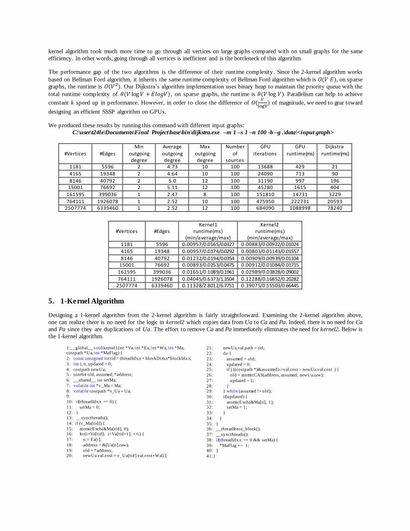
kernel algorithm took much more time to go through all vertices on large graphs compared with on small graphs for the same

efficiency. In other words, going through all vertices is inefficient and is the bottleneck of this algorithm.

The performance gap of the two algorithms is the difference of their runtime complexity. Since the 2-kernel algorithm works

based on Bellman Ford algorithm, it inherits the same runtime complexity of Bellman Ford algorithm which is , on sparse

graphs, the runtime is . Our Dijkstra’s algorithm implementation uses binary heap to maintain the priority queue with the

total runtime complexity of , on sparse graphs, the runtime is . Parallelism can help to achieve

constant k speed up in performance. However, in order to close the difference of

of magnitude, we need to gear toward

designing an efficient SSSP algorithm on GPUs.

We produced these results by running this command with different input graphs:

C:\user\t24le\Documents\Final Project\base\bin\dijkstra.exe –m 1 –s 1 –n 100 -b –g .\data\<input graph>

#Vertices

#Edges

Min

outgoing degree

Average

outgoing degree

Max

outgoing degree

Number

of sources

GPU

iterations

GPU

runtime(ms)

Dijkstra

runtime(ms)

1181 5596 2 4.73 10 100 13688 429 21

4165 19348 2 4.64 10 100 24090 713 90

8146 40792 2 5.0 12 100 31190 997 196 15001 76692 2 5.11 12 100 45280 1615 404

161595 399036 1 2.47 8 100 151810 14731 3229

764111 1926078 1 2.52 10 100 475950 222731 20593 2507774 6339460 1 2.52 12 100 684090 1088998 78240

#Vertices

#Edges Kernel1

runtime(ms) (min/average/max)

Kernel2 runtime(ms)

(min/average/max) 1181 5596 0.00957/0.0165/0.0327 0.00883/0.00922/0.01024

4165 19348 0.00957/0.0174/0.0292 0.00803/0.01143/0.01557

8146 40792 0.01232/0.0194/0.0354 0.00909/0.00939/0.01104 15001 76692 0.00893/0.0253/0.0475 0.00912/0.01084/0.01715

161595 399036 0.01651/0.1089/0.1961 0.02989/0.03828/0.09002

764111 1926078 0.04045/0.6373/1.3504 0.12288/0.16852/0.20282 2507774 6339460 0.11328/2.8012/6.7751 0.39075/0.55503/0.66445

5. 1-Kernel Algorithm

Designing a 1-kernel algorithm from the 2-kernel algorithm is fairly straightforward. Examining the 2-kernel algorithm above,

one can realize there is no need for the logic in kernel2 which copies data from Ua to Ca and Pa. Indeed, there is no need for Ca

and Pa since they are duplications of Ua. The effort to remove Ca and Pa immediately eliminates the need for kernel2. Below is

the 1-kernel algorithm.

1:__global__ void kernel1(int *Va, int *Ea, int *Wa, int *Ma, costpath *Ua, int *MaFlag) {

2: const unsigned int tid = threadIdx.x + blockDim.x*blockIdx.x;

3: int i, n, updated = 0;

4: costpath newUa; 5: uint64 old, assumed, *address;

6: __shared__ int setMa;

7: volatile int *v_Ma = Ma;

8: volatile costpath *v_Ua = Ua; 9:

10: if(threadIdx.x == 0) {

11: setMa = 0;

12: } 13: __syncthreads();

14: if (v_Ma[tid]) {

15: atomicExch(&Ma[tid], 0); 16: for(i=Va[tid]; i<Va[tid+1]; ++i) {

17: n = Ea[i];

18: address = &(Ua[n].raw);

19: old = *address; 20: newUa.val.cost = v_Ua[tid].val.cost+Wa[i];

At line 6, we declare the shared variable setMa for each thread block. In the while loop at line 22, we set the local variable

updated if the condition at line 25 is satisfied. It means every time a vertex has its shortest distance and path updated, the local

variable updated will be set by the thread performing this update. Once the while loop is complete, threads who have the local variable updated set update the corresponding value of the updated vertex in Ma array and the shared variable setMa accordingly.

At line 38, the first thread in each thread block examines the value stored in the shared variable setMa and increments the global

MaFlag if setMa is set. By doing that, kernel1 is now taking the responsibility of kernel2 in maintaining Ma array and MaFlag,

Hence, kernel2 can be removed. On the host, we only need to keep track of the previous value of MaFlag and the current value of

MaFlag. If they are the same, the algorithm is complete and the execution is terminated. If they are different, the algorithm continues to the next iteration. It is noteworthy to mention in the 1-kernel algorithm, we need to use the volatile key work for

local variables v_Ma and v_Ua referencing Ma and Ua in global memory respectively. Every memory access to Ma and Ua

should make reference to these two local variables to avoid reading stale data due to the lack of full cache coherence in CUDA.

Verification

We run the same verification step for this algorithm. Below is the summary of running the algorithm in verification mode.



Performance Results

By reducing to one kernel, the 1-kernel algorithm performs an order of magnitude faster than the 2-kernel algorithm. Since it is

still based on the inefficient approach, the performance is still incomparable with the performance of Dijstra’s algorithm.


C:\user\t24le\Documents\Final Project\base1Kernel\bin\dijkstra.exe –m 1 –s 1 –n 100 -b –g .\data\<input graph>

C:\Users\t24le\Documents\Final Project\base1Kernel\bin>dijkstra.exe -s 1 -m 0 -n 100 -b -g .\data\15K.txt

Graph from file: .\data\15K.txt SPT on 15001 nodes, 76692 edges with 100 source(s)

Running source(s): 41 3466 6334 11499 4168 ...


Min degree 2

Max degree 12

Average degree 5.11246 Num edge repeats 38346


-------------------------------------------------- ------

SUMMARY:

100 out of 100 source node DISTANCES match. 100 out of 100 source node GPU PATH LENGTHS correct.

100 out of 100 source node CPU PATH LENGTHS correct.

0 out of 100 source node PATHS match.


Alloc & input graph h->d input 0.96253 ms Set up new source h->d input 20.28327 ms

Kernel execution d 460.91846 ms

Min kernel execution d 0.00918 ms

Max kernel execution d 0.11069 ms Average kernel execution d 0.02075 ms

Total kernel execution d 460.91846 ms

Synchronize d 202.29326 ms

Ma reads d->h transfer 313.67926 ms Read results d->h transfer 10.03107 ms

-------------

GPU KERNEL TIME with respect to CUDA d 1008.16785 ms -------------

GPU TOTAL TIME with respect to CPU h+d 1648.47351 ms

-------------


-------------------------------------------------- ------

#Vertices

#Edges

Min outgoing

degree

Average outgoing

degree

Max outgoing

degree

Source

Vertex

GPU iterations

GPU runtime(ms)

Dijkstra runtime(ms)

1181 5596 2 4.73 10 100 6515 283 21

4165 19348 2 4.64 10 100 11809 552 90

8146 40792 2 5.0 12 100 15386 720 196 15001 76692 2 5.11 12 100 22206 1043 404

161595 399036 1 2.47 8 100 45089 6070 3229

764111 1926078 1 2.52 10 100 123058 106049 20593 2507774 6339460 1 2.52 12 100 172711 588081 78240

#Vertices

#Edges Kernel


1181 5596 0.01037/0.01791/0.08688

4165 19348 0.01325/0.01918/0.03213

8146 40792 0.01277/0.01954/0.07811 15001 76692 0.01181/0.02175/0.04506

161595 399036 0.01885/0.10425/0.21123

764111 1926078 0.05789/0.78669/1.59840 2507774 6339460 0.17370/3.56861/8.91002

6. Warp-Based Algorithm

Warp-based methodology described in [4] can be incorporated into the 1-kernel algorithm to achieve better performance. The advantages of the warp-based approach are two-fold: better coalescing memory and avoiding thread divergence.

From line 2 – line 4, the algorithm computes the number of virtual warps within a thread block, the warp id for the current thread, the thread offset of the current thread within its virtual warp and the warp offset with respect to the entire grid. Using the warp

offset calculated at line 4, the algorithm moves the pointers of Va, Ma and Ua to the correct position for each virtual warp. After

finishing line 7, every virtual warp accesses Va, Ma and Ua at different positions. The calculation done at line 4 makes sure

virtual warps work on different chunks of data in global memory and there is no overlapping work among virtual warps. Line 8 &

9 declare the shared memory for each virtual warp in a thread block. Each virtual warp has a slot in this shared memory with the size equal to CHUNK_SZ. From line 18 – line 23, each thread in a virtual warp copies data from Ma and Va to its shared

memory slot. These instructions are executed in SIMD phase. At line 26, the for loop will go through all data previously stored in

1:__global__ void kernel1Warp(int *Va, int *Ea, int *Wa,

int *Ma, costpath *Ua, int *MaFlag) { 2: int warp_nums = blockDim.x / WARP_SZ, warp_id = threadIdx.x / WARP_SZ;

3: int thread_offset = threadIdx.x % WARP_SZ;

4: int warp_offset = warp_id * CHUNK_SZ + blockIdx.x * warp_nums * CHUNK_SZ;

5: int * w_Va = Va + warp_offset, * w_Ea, * w_Wa; 6: volatile int * v_Ma = Ma + warp_offset;

7: volatile costpath * v_Ua = &Ua[warp_offset];

8: __shared__ int comm_Ma[THREADS_IN_BLOCK / WARP_SZ][CHUNK_SZ];

9: __shared__ int comm_Va[THREADS_IN_BLOCK / WARP_SZ][CHUNK_SZ + 1]; 10: __shared__ int setMa;

11: int i, j, neighbor, updated = 0, start, cnt, weight;

12: costpath newUa; 13: uint64 old, assumed, *address;

14:

15: if(threadIdx.x == 0) {

16: setMa = 0; 17: }

18: for(i = thread_offset; i < CHUNK_SZ; i += WARP_SZ) {

19: comm_Ma[warp_id][i] = v_Ma[i];

20: } 21: for(i = thread_offset; i < CHUNK_SZ + 1; i += WARP_SZ) {

22: comm_Va[warp_id][i] = w_Va[i];

23: }

24: __threadfence_block(); 25: __syncthreads();

26: for(i = 0; i < CHUNK_SZ; i++) {

27: if (comm_Ma[warp_id][i]) { 28: if(thread_offset == 0) {

29: atomicExch(&Ma[i + warp_offset], 0);

30: }

31: start = comm_Va[warp_id][i];

32: cnt = comm_Va[warp_id][i + 1] - start;

33: w_Ea = Ea + start; 34: w_Wa = Wa + start;

35: for(j = thread_offset; j < cnt; j += WARP_SZ) {

36: neighbor = w_Ea[j]; 37: weight = w_Wa[j];

38: address = &(Ua[neighbor].raw);

39: old = *address;

40: newUa.val.cost = v_Ua[i].val.cost + weight; 41: newUa.val.path = i + warp_offset;

42: do {

43: assumed = old;

44: updated = 0; 45: if (((costpath *)&assumed)->val.cost > newUa.val.cost) {

46: old = atomicCAS(address, assumed, newUa.raw);

47: updated = 1;

48: } 49: } while (assumed != old);

50: if(updated) {

51: atomicExch(&Ma[neighbor], 1); 52: setMa = 1;

53: }

54: }

55: } 56: }

57: __threadfence_block();


59: if(threadIdx.x == 0 && setMa) { 60: atomicAdd(MaFlag, 1);

61: }

62:}

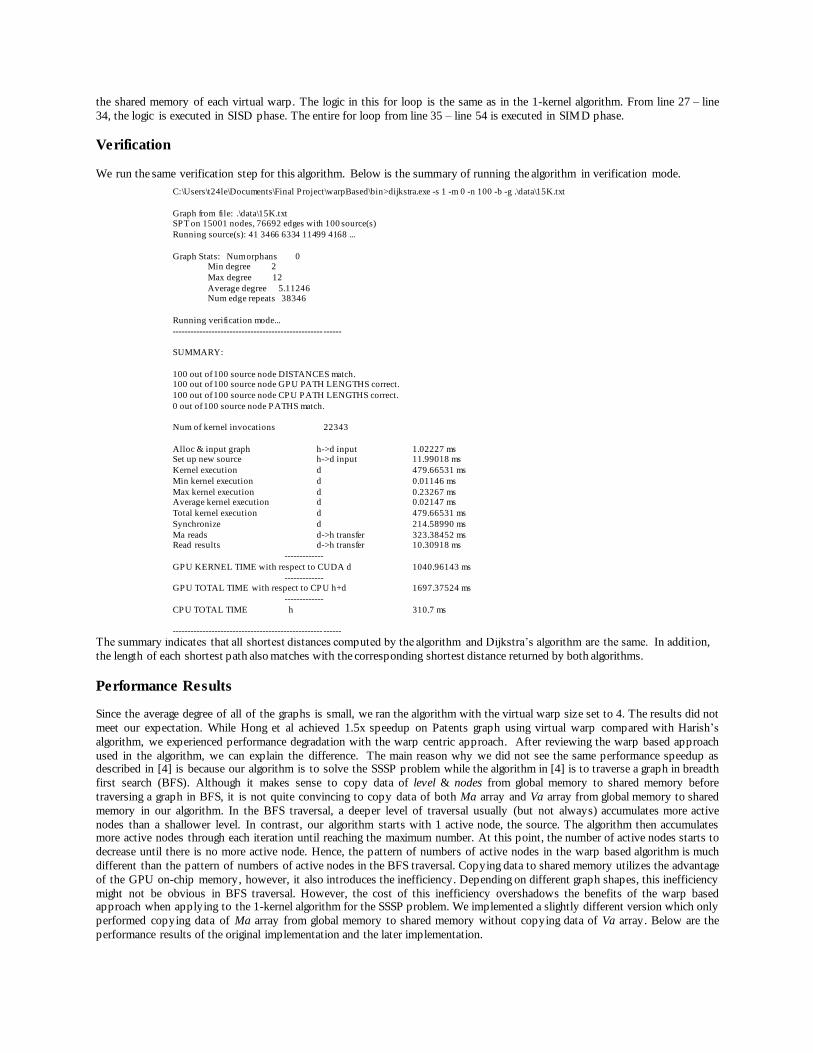
the shared memory of each virtual warp. The logic in this for loop is the same as in the 1-kernel algorithm. From line 27 – line

34, the logic is executed in SISD phase. The entire for loop from line 35 – line 54 is executed in SIMD phase.

Verification




Performance Results

Since the average degree of all of the graphs is small, we ran the algorithm with the virtual warp size set to 4. The results did not

meet our expectation. While Hong et al achieved 1.5x speedup on Patents graph using virtual warp compared with Harish’s

algorithm, we experienced performance degradation with the warp centric approach. After reviewing the warp based approach

used in the algorithm, we can explain the difference. The main reason why we did not see the same performance speedup as described in [4] is because our algorithm is to solve the SSSP problem while the algorithm in [4] is to traverse a graph in breadth

first search (BFS). Although it makes sense to copy data of level & nodes from global memory to shared memory before

traversing a graph in BFS, it is not quite convincing to copy data of both Ma array and Va array from global memory to shared

memory in our algorithm. In the BFS traversal, a deeper level of traversal usually (but not always) accumulates more active

nodes than a shallower level. In contrast, our algorithm starts with 1 active node, the source. The algorithm then accumulates more active nodes through each iteration until reaching the maximum number. At this point, the number of active nodes starts to

decrease until there is no more active node. Hence, the pattern of numbers of active nodes in the warp based algorithm is much

different than the pattern of numbers of active nodes in the BFS traversal. Copying data to shared memory utilizes the advantage

of the GPU on-chip memory, however, it also introduces the inefficiency. Depending on different graph shapes, this inefficiency

might not be obvious in BFS traversal. However, the cost of this inefficiency overshadows the benefits of the warp based approach when applying to the 1-kernel algorithm for the SSSP problem. We implemented a slightly different version which only

performed copying data of Ma array from global memory to shared memory without copying data of Va array. Below are the

performance results of the original implementation and the later implementation.

C:\Users\t24le\Documents\Final Project\warpBased\bin>dijkstra.exe -s 1 -m 0 -n 100 -b -g .\data\15K.txt

Graph from file: .\data\15K.txt SPT on 15001 nodes, 76692 edges with 100 source(s)

Running source(s): 41 3466 6334 11499 4168 ...

Graph Stats: Num orphans 0 Min degree 2

Max degree 12

Average degree 5.11246 Num edge repeats 38346


-------------------------------------------------- ------

SUMMARY:

100 out of 100 source node DISTANCES match. 100 out of 100 source node GPU PATH LENGTHS correct.

100 out of 100 source node CPU PATH LENGTHS correct.



Alloc & input graph h->d input 1.02227 ms Set up new source h->d input 11.99018 ms

Kernel execution d 479.66531 ms

Min kernel execution d 0.01146 ms

Max kernel execution d 0.23267 ms Average kernel execution d 0.02147 ms

Total kernel execution d 479.66531 ms


Ma reads d->h transfer 323.38452 ms Read results d->h transfer 10.30918 ms

-------------


------------- GPU TOTAL TIME with respect to CPU h+d 1697.37524 ms

-------------


-------------------------------------------------- ------


C:\user\t24le\Documents\Final Project\warpBased\bin\dijkstra.exe –m 1 –s 1 –n 100 -b –g .\data\<input graph>

7. Queue-Based Algorithm

Queue-based algorithm was our first effort toward a work-efficient algorithm for the SSSP problem on GPUs. Thus far, none of

above algorithm can be comparable with Dijkstra’s algorithm. The queue based algorithm runs with two queues. Each queue is

allocated with a size equals to the number of vertices. The kernel logic works from the current queue, any vertex has its shortest

distance and path updated is added into the next queue. The rest of the logic is the same as of the warp-based algorithm. For better utilizing shared memory, the algorithm keeps all new updated vertices in shared memory and writes these vertices out to

6567 6393 7649

10490

17014

0

2000

4000

6000

8000

10000

12000

14000

16000

18000

CHUNK 4 CHUNK 8 CHUNK 16 CHUNK 32 CHUNK 64

#Vertices

#Edges

Min outgoing degree

Average outgoing degree

Max outgoing degree

Number Source Vertex

Virtual Warp Size

Chunk size

GPU iterations

GPU Runtime

(ms)

Dijkstra Runtime

(ms)

1181 5596 2 4.73 10 100 4 4 6572 292 21 4165 19348 2 4.64 10 100 4 4 11858 527 90

8146 40792 2 5.0 12 100 4 4 15428 669 196

15001 76692 2 5.11 12 100 4 4 22335 1092 404 161595 399036 1 2.47 8 100 4 4 44014 6386 3229

764111 1926078 1 2.52 10 100 4 4 122335 102140 20593

2507774 6339460 1 2.52 12 100 4 4 172521 561129 78240

#Vertices

#Edges

Min outgoing degree


Max outgoing degree

Number Source Vertex

Virtual Warp Size

Chunk size

GPU iterations

GPU Runtime

(ms)

Dijkstra Runtime

(ms)

1181 5596 2 4.73 10 100 4 4 6572 263 21

4165 19348 2 4.64 10 100 4 4 11857 485 90 8146 40792 2 5.0 12 100 4 4 15423 649 196

15001 76692 2 5.11 12 100 4 4 22338 977 404

161595 399036 1 2.47 8 100 4 4 43730 6259 3229

764111 1926078 1 2.52 10 100 4 4 122114 103490 20593 2507774 6339460 1 2.52 12 100 4 4 172434 574918 78240

#Vertices

#Edges

Kernel runtime(ms)

(min/average/max)

1181 5596 0.01107/0.01651/0.02976

4165 19348 0.01139/0.01894/0.12835 8146 40792 0.01178/0.01859/0.03350

15001 76692 0.01235/0.02091/0.03530

161595 399036 0.03994/0.10806/0.19312 764111 1926078 0.16170/0.74485/1.51683

2507774 6339460 0.51315/3.46111/8.73542

Performance results of warp based algorithm copying data of Ma and Va to shared memory

Performance results of warp based algorithm copying data of Ma to shared memory

Effect of different chunk sizes

#Vertices: 161595 #Edges: 399036

global memory as a whole in SIMD phase (line 64 – line 72). We found this is a simpler way than the prefix sum for coordinating

allocation described in [5]. The atomicAdd at line 66 suffers a minimal overhead from lock contention due to only the first thread

of each virtual warp performs this atomic operation. The host logic needs to examine the value stored in nextSize. If the value is 0, it indicates there are no more vertices in the next queue. At this point, the algorithm is complete and the execution is

terminated. Otherwise, the host logic launches a new kernel and swaps the current queue with the next queue.

Verification


1:__global__ void kernel1Queue(int *Va, int *Ea, int *Wa, int *Ma, costpath *Ua,

2: int * curQueue, int * curSize, int * nextQueue, int * nextSize) { 3: int warp_nums = blockDim.x / WARP_SZ, warp_id = threadIdx.x / WARP_SZ;



6: int updated = 0, vertex, cnt, i, j, start, neighbor, weight, pos, *w_nextQueue, *w_Ea, *w_Wa; 7: costpath newUa;

8: uint64 old, assumed, *address;

9: int * d_curQueue = curQueue + warp_offset; 10: volatile int * v_Ma = Ma;

11: volatile costpath * v_Ua = Ua;

12: __shared__ int curFront[THREADS_IN_BLOCK / WARP_SZ][CHUNK_SZ];

13: __shared__ int nextFront[THREADS_IN_BLOCK / WARP_SZ][MAX_DEGREE * CHUNK_SZ]; 14: __shared__ int position[THREADS_IN_BLOCK / WARP_SZ][1];

15: if(warp_offset < *curSize) {

16: int amount = *curSize - warp_offset;

17: if(amount > CHUNK_SZ) { 18: amount = CHUNK_SZ;

19: }

20: if(thread_offset == 0) {

21: position[warp_id][0] = 0; 22: }


24: for(i = thread_offset; i < amount; i += WARP_SZ) { 25: vertex = d_curQueue[i];

26: if(v_Ma[vertex]) {

27: pos = atomicAdd(position[warp_id], 1);

28: curFront[warp_id][pos] = d_curQueue[i]; 29: atomicExch(&Ma[vertex], 0);

30: }

31: }

32: __syncthreads(); 33: amount = position[warp_id][0];

34: for(i = 0; i < amount; i++) {

35: if(thread_offset == 0) {

36: position[warp_id][0] = 0; 37: }

C:\Users\t24le\Documents\Final Project\queueBased\bin>dijkstra.exe -s 1 -m 0 -n 100 -b -g .\data\15K.txt


SPT on 15001 nodes, 76692 edges with 100 source(s)

Running source(s): 41 3466 6334 11499 4168 ...


Min degree 2

Max degree 12 Average degree 5.11246



-------------------------------------------------- ------

SUMMARY:


100 out of 100 source node GPU PATH LENGTHS correct.

100 out of 100 source node CPU PATH LENGTHS correct. 0 out of 100 source node PATHS match.




Kernel execution d 1251.53223 ms Min kernel execution d 0.00970 ms

Max kernel execution d 0.08541 ms

Average kernel execution d 0.05620 ms

Total kernel execution d 1251.53223 ms Synchronize d 198.15681 ms


38: vertex = curFront[warp_id][i];

39: start = Va[vertex]; 40: cnt = Va[vertex + 1] - start;

41: w_Ea = Ea + start;

42: w_Wa = Wa + start;

43: for(j = thread_offset; j < cnt; j += WARP_SZ) { 44: neighbor = w_Ea[j];

45: weight = w_Wa[j];

46: address = &(Ua[neighbor].raw); 47: old = *address;

48: newUa.val.cost = v_Ua[vertex].val.cost + weight;

49: newUa.val.path = vertex;

50: do { 51: assumed = old;

52: updated = 0;

53: if (((costpath *)&assumed)->val.cost > newUa.val.cost) {

54: old = atomicCAS(address, assumed, newUa.raw); 55: updated = 1;

56: }

57: } while (assumed != old);

58: if(updated && !v_Ma[neighbor]) { 59: atomicExch(&Ma[neighbor], 1);


61: nextFront[warp_id][pos] = neighbor; 62: }

63: }

64: int size = position[warp_id][0];

65: if(thread_offset == 0 && size > 0) { 66: position[warp_id][0] = atomicAdd(nextSize, size);

67: }


69: w_nextQueue = nextQueue + position[warp_id][0]; 70: for(j = thread_offset; j < size; j += WARP_SZ) {

71: w_nextQueue[j] = nextFront[warp_id][j];

72: }

73: } 74: }

75:}

The summary indicates that all shortest distances computed by the algorithm and Dijkstra’s algorithm are the same. In addition, the length of each shortest path also matches with the corresponding shortest distance returned by both algorithms.

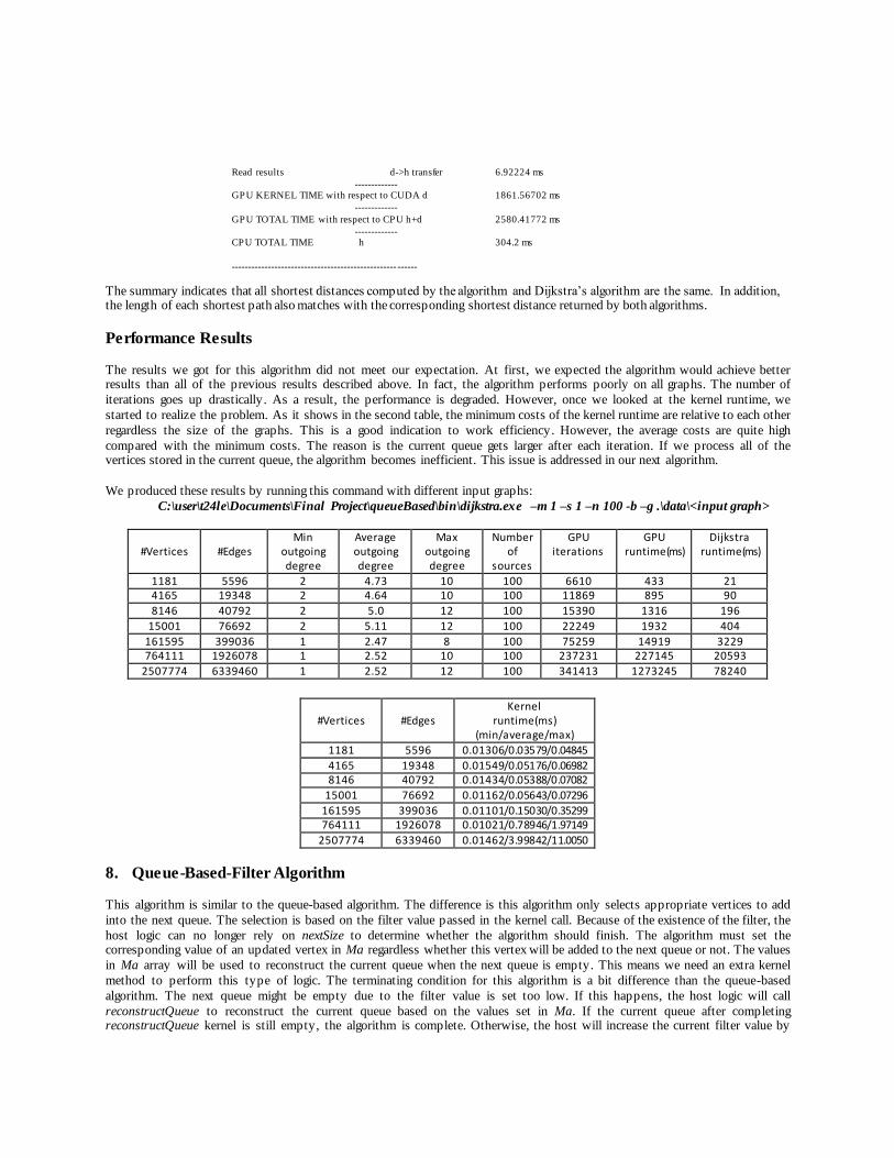
Performance Results

The results we got for this algorithm did not meet our expectation. At first, we expected the algorithm would achieve better results than all of the previous results described above. In fact, the algorithm performs poorly on all graphs. The number of

iterations goes up drastically. As a result, the performance is degraded. However, once we looked at the kernel runtime, we

started to realize the problem. As it shows in the second table, the minimum costs of the kernel runtime are relative to each other

regardless the size of the graphs. This is a good indication to work efficiency. However, the average costs are quite high

compared with the minimum costs. The reason is the current queue gets larger after each iteration. If we process all of the vertices stored in the current queue, the algorithm becomes inefficient. This issue is addressed in our next algorithm.


C:\user\t24le\Documents\Final Project\queueBased\bin\dijkstra.exe –m 1 –s 1 –n 100 -b –g .\data\<input graph>

#Vertices

#Edges

Min outgoing degree


Max outgoing degree

Number of

sources

GPU iterations

GPU runtime(ms)


1181 5596 2 4.73 10 100 6610 433 21 4165 19348 2 4.64 10 100 11869 895 90

8146 40792 2 5.0 12 100 15390 1316 196

15001 76692 2 5.11 12 100 22249 1932 404

161595 399036 1 2.47 8 100 75259 14919 3229 764111 1926078 1 2.52 10 100 237231 227145 20593

2507774 6339460 1 2.52 12 100 341413 1273245 78240

#Vertices

#Edges Kernel


1181 5596 0.01306/0.03579/0.04845

4165 19348 0.01549/0.05176/0.06982 8146 40792 0.01434/0.05388/0.07082

15001 76692 0.01162/0.05643/0.07296

161595 399036 0.01101/0.15030/0.35299 764111 1926078 0.01021/0.78946/1.97149

2507774 6339460 0.01462/3.99842/11.0050

8. Queue-Based-Filter Algorithm

This algorithm is similar to the queue-based algorithm. The difference is this algorithm only selects appropriate vertices to add

into the next queue. The selection is based on the filter value passed in the kernel call. Because of the existence of the filter, the

host logic can no longer rely on nextSize to determine whether the algorithm should finish. The algorithm must set the corresponding value of an updated vertex in Ma regardless whether this vertex will be added to the next queue or not. The values

in Ma array will be used to reconstruct the current queue when the next queue is empty. This means we need an extra kernel

method to perform this type of logic. The terminating condition for this algorithm is a bit difference than the queue-based

algorithm. The next queue might be empty due to the filter value is set too low. If this happens, the host logic will call

reconstructQueue to reconstruct the current queue based on the values set in Ma. If the current queue after completing reconstructQueue kernel is still empty, the algorithm is complete. Otherwise, the host will increase the current filter value by

Read results d->h transfer 6.92224 ms

------------- GPU KERNEL TIME with respect to CUDA d 1861.56702 ms

-------------

GPU TOTAL TIME with respect to CPU h+d 2580.41772 ms

------------- CPU TOTAL TIME h 304.2 ms

-------------------------------------------------- ------

and the algorithm continues with this new filter value. Due to time constraint, we have not come up with a

general formula to choose a proper constant for the algorithm. This will be included in our future work.

Recently, we have discovered that our queue-base filter algorithm is similar to the threshold shortest path algorithm [1]. It is

interesting to learn the general approach described in [1] for determining a suitable threshold value in the threshold shortest path algorithm.

Verification


1:__global__ void scatteringKernel(int *Va, int *Ea, int *Wa, int *Ma, costpath *Ua,

2: int * curQueue, int * curSize, int * nextQueue, int * nextSize, int * filter) {

…. …. 58: if(updated && !v_Ma[neighbor]) { 59: atomicExch(&Ma[neighbor], 1);

60: if(newUa.val.cost <= filterVal) {


62: nextFront[warp_id][pos] = neighbor; 63: }

64: }

… …

1:__global__ void reconstructQueue(int *Ma, int * curQueue, int * curSize) {

2: int warp_nums = blockDim.x / WARP_SZ; 3: int warp_id = threadIdx.x / WARP_SZ;



6: int pos = 0, i, size, *w_curQueue; 7: volatile int * v_Ma = Ma + warp_offset;

8: __shared__ int frontier[256 / WARP_SZ][CHUNK_SZ];

9: __shared__ int position[256 / WARP_SZ][1]; 10: if(thread_offset == 0) {

11: position[warp_id][0] = 0;

12: }

13: __syncthreads(); 14: for(i = thread_offset; i < CHUNK_SZ; i += WARP_SZ) {

15: if (v_Ma[i]) {


17: frontier[warp_id][pos] = warp_offset + i; 18: }

19: }

20: __syncthreads(); 21: size = position[warp_id][0];

22: if(thread_offset== 0 && size > 0) {

23: pos = atomicAdd(curSize, size);

24: position[warp_id][0] = pos; 25: }


27: pos = position[warp_id][0];

28: w_curQueue = curQueue + pos; 29: for(i = thread_offset; i < size; i += WARP_SZ) {

30: w_curQueue[i] = frontier[warp_id][i];

31: }

32:}

C:\Users\t24le\Documents\Final Project\queueBasedFilter\bin>dijkstra.exe -s 1 –m 0 -n 100 -K 100 -b -g .\data\15K.txt


SPT on 15001 nodes, 76692 edges with 100 source(s) Running source(s): 41 3466 6334 11499 4168 ...


Min degree 2 Max degree 12

Average degree 5.11246



-------------------------------------------------- ------

SUMMARY:


100 out of 100 source node GPU PATH LENGTHS correct. 100 out of 100 source node CPU PATH LENGTHS correct.





Kernel execution d 1255.09021 ms Min kernel execution d 0.00992 ms

Max kernel execution d 0.08352 ms

Average kernel execution d 0.05624 ms Total kernel execution d 1255.09021 ms



Read results d->h transfer 6.81235 ms

Performance Results

This algorithm truly demonstrates the work-efficient advantage which results in much better performance on large graphs

compared with all of the above results. The GPU runtime of this algorithm is comparable with Dijkstra’s algorithm. On larger graphs, this algorithm might outperform Dijkstra’s algorithm.


C:\user\t24le\Documents\Final Project\queueBasedFilter\bin\dijkstra.exe –m 1 –s 1 –n 100 –K <k-value> -b –g

.\data\<input graph>

#Vertices

#Edges

Min outgoing degree


Max outgoing degree

Source Vertex

K

GPU iterations

GPU runtime(ms)


1181 5596 2 4.73 10 100 40 6711 435 21 4165 19348 2 4.64 10 100 60 11960 918 90

8146 40792 2 5.0 12 100 80 15496 1263 196

15001 76692 2 5.11 12 100 100 22335 1930 404 161595 399036 1 2.47 8 100 120 109068 9290 3229

764111 1926078 1 2.52 10 100 60 508063 41599 20593

2507774 6339460 1 2.52 12 100 400 760530 77734 78240

#Vertices

#Edges Kernel


1181 5596 0.01350/0.03563/0.04931 4165 19348 0.01546/0.05147/0.06934

8146 40792 0.01386/0.05367/0.07222

15001 76692 0.01235/0.05630/0.07485 161595 399036 0.01053/0.06093/0.13030

764111 1926078 0.01046/0.05622/0.10138

2507774 6339460 0.01043/0.07226/0.22086

9. Conclusion

Our report shows a step by step on how to design an efficient algorithm for the SSSP problem on GPUs. Initially, we started with

the basic algorithm and focused on the correctness. We then made incremental improvement on each new algorithm over the current algorithm. The 1-kernel algorithm was an important achievement in our study. It helped us to design a new algorithm

much easier with less effort in troubleshooting. Our report emphasizes the importance of work efficiency in designing an

algorithm on GPUs. As we have shown, the queue-based filter algorithm is the only algorithm comparable with Dijkstra’s

algorithm in term of performance. There is still room for improvement on this algorithm. We did not incorporate pinned/mapped

memory into the implementation. Using pinned/mapped memory might produce slightly better performance. Another improvement would be instead of adding updated vertices into the next queue, it might be better to first add them into the current

queue until the current queue is full then the algorithm can start to add next updated vertices to the next queue.

References

[1] M.J. Flynn. Some Computer Organizations and Their Effectiveness. IEEE Trans. Computers, C-21, No.9, pp. 948-960, 1972.

[2] Fred Glover, Randy Glover and Darwin Klingman. Threshold Assignment Algorithm. Mathematical Programming Studies,

Volumn 26, 12-37, 1986.

[3] Pawan Harish and P.J. Narayanan. Accelerating Large Graph Algorithms on the GPU Using CUDA. HiPC 2007, LNCS 4873, 197-208, 2007.


-------------

GPU TOTAL TIME with respect to CPU h+d 2538.07373 ms -------------


-------------------------------------------------- ------

[4] Sungpack Hong, Sang Kyun Kim, Tayo Uguntebi and Kunle Olukotun. Accelerating CUDA Graph Algorithm at Maximum

Graph, Proceedings of the 16th ACM symposium on Principles and practice of parallel programming, February 12-16, 2011, San

Antonio, TX, USA.

[5] Duane Merrill, Michael Garland, Andrew Grimshaw. Scalable GPU Graph Traversal. Proceeding PPoP ’12, February 25-29,

2012, New Orleans, Louisiana, USA.

toward an efficient algorithm for the single source shortest path problem on gpus

Documents

efficient algorithm

bellman ford algorithm

gpus thang

gpus architecture

classical problem

multiple vertices

number of vertices

gpu global memory