toward a fully parametric retrieval of the nonraining parameters over the global oceans

Toward a Fully Parametric Retrieval of the Nonraining Parameters over theGlobal Oceans

GREGORY S. ELSAESSER AND CHRISTIAN D. KUMMEROW

Department of Atmospheric Science, Colorado State University, Fort Collins, Colorado

(Manuscript received 5 February 2007, in final form 4 September 2007)

ABSTRACT

In light of the upcoming launch of the Global Precipitation Measurement (GPM) mission, a parametricretrieval algorithm of the nonraining parameters over the global oceans is developed with the ability toaccommodate all currently existing and planned spaceborne microwave window channel sensors and im-agers. The physical retrieval is developed using all available sensor channels in a full optimal estimationinversion. This framework requires that retrieved parameters be physically consistent with all observedsatellite radiances regardless of the sensor being used. The retrieval algorithm has been successfully appliedto the Advanced Microwave Scanning Radiometer-Earth Observing System (AMSR-E), the Special SensorMicrowave Imager (SSM/I), and the Tropical Rainfall Measuring Mission (TRMM) Microwave Imager(TMI) with geophysical parameter retrieval results comparable to independent studies using sensor-optimized algorithms. The optimal estimation diagnostics characterize the retrieval further, providing errorsassociated with each of the retrieved parameters, indicating whether the retrieved state is physically con-sistent with observed radiances, and yielding information on how well simulated radiances agree withobserved radiances. This allows for the quantitative assessment of potential calibration issues in either themodel or sensor. In addition, there is an expected, consistent response of these diagnostics based on thescene being observed, such as in the case of a raining scene, allowing for the emergence of a rainfalldetection scheme providing a new capability in rainfall identification for use in passive microwave rainfalland cloud property retrievals.

1. Introduction

The upcoming Global Precipitation Measurement(GPM) mission will incorporate a constellation of ex-isting operational and dedicated spaceborne microwaveradiometers with the goal of studying global precipita-tion, a key component of the earth’s hydrological cycle.To achieve consistent global precipitation productsamong a number of sensors, a rainfall algorithm isneeded to parametrically accommodate any passive mi-crowave sensor in orbit. As improvements in both thenumber of channels, field-of-view resolution, and cali-bration of spaceborne radiometers have been made,algorithm development thus far has largely been fo-cused on the latest sensor (Shin and Kummerow 2003).As such, efforts to produce consistent, homogenous

geophysical products for long time series are impededdue to sensor-specific assumptions associated with sen-sor-specific algorithms. It is necessary, therefore, thatalgorithms be developed so that the issues of inconsis-tency in the geophysical parameter products from a di-verse range of spaceborne sensors can be addressed.

Shin and Kummerow (2003) first made progress onthis front by constructing a parametric rainfall retrievalalgorithm within a Bayesian framework used in con-junction with a coupled Tropical Rainfall MeasuringMission (TRMM) precipitation radar (PR) and cloud-resolving model (CRM) a priori database. They re-trieved the most likely hydrometeor profile with theassurance that simulated brightness temperatures cor-responding to the retrieved profile agreed with ob-served (synthetic) brightness temperatures. Masunagaand Kummerow (2005) made further progress by allow-ing for variation in the drop size distribution (DSD)and ice density assumed by a TRMM PR algorithm toachieve the best agreement between simulated and ob-served brightness temperatures. However, brightness

Corresponding author address: Gregory Elsaesser, Dept. of At-mospheric Science, Colorado State University, Fort Collins, CO80523-1371.E-mail: [email protected]

JUNE 2008 E L S A E S S E R A N D K U M M E R O W 1599

DOI: 10.1175/2007JAMC1712.1

© 2008 American Meteorological Society

JAMC1712

temperature discrepancies remain and uncertaintiesstill exist.

Kummerow et al. (2006) quantified a number ofthese uncertainties using a simple rainfall algorithm. Ina physical rainfall retrieval algorithm, rainfall estima-tion errors arise not only from assumptions in the apriori database, but also from errors in the nonrainingscene. These errors are introduced from uncertainty inthe nonraining parameters [column-integrated watervapor (TPW), surface wind (WIND), and integratedcloud liquid water (LWP)], as well as from errors aris-ing from changes in rain–no-rain thresholds (Kum-merow et al. 2006). Since a three-dimensional rainfallstructure consistent with all brightness temperatures isdesired, there must be assurance that the nonrainingscene is also consistent with brightness temperatures,independent of the microwave sensor being utilized,since both errors in the retrieved precipitation profileand errors in the nonraining scene contribute to thetotal brightness temperature error. Just as there is aneed for a parametric rainfall algorithm for GPM, sothere is a need for a parametric nonraining algorithm.

The parametric algorithms being designed for GPMmust also provide a full description of the errors in theretrieval. One such uncertainty arises during the rain–no-rain discrimination process. One needs to know thecontribution to the brightness temperature from thenonprecipitating component of the cloud in order toassess the contribution from the precipitating compo-nent. The ability to detect rain within the radiometer-only retrieval framework, while most problematic overland, remains a significant issue over the ocean. Ferraroet al. (1998) discussed a number of discriminationmethods involving brightness temperature thresholds,while acknowledging the difficulty of finding an algo-rithm that works equally well globally. Berg et al.(2006) noted that a liquid water path threshold is typi-cally used in microwave radiometry for rainfall detec-tion. They showed that this can lead to rainfall retrievaldiscrepancies in regions where nonraining, high LWPclouds may exist because of possible aerosol interactiondelaying the onset of precipitation, such as over theEast China Sea. There is, then, the desire to have analgorithm that has both the ability to assess the uncer-tainty in the nonraining parameters and the capabilityof discriminating raining clouds from nonraining clouds.

The objective of this study is not to develop a newnonraining retrieval, but instead to develop a frame-work that facilitates the merger of parametric back-ground retrievals with rainfall retrievals allowing for acoherent atmospheric description to emerge within theGPM framework consistent with all observed bright-

ness temperatures. To this end, the framework used forretrieving the nonraining parameters must not be de-pendent on a particular channel or empirical adjust-ments that would be unique to an algorithm optimizedfor a particular sensor. Instead, it should be designedsuch that it is portable to any microwave window chan-nel radiometer. The physical algorithm is developedwithin the optimal estimation framework. The benefitsof optimal estimation can be summarized as providingfully parametric retrievals necessary for GPM, associ-ated error estimates, and retrieval diagnostics. It is im-portant to note that while a unified algorithm for rain-ing and nonraining scenes within an optimal estimationframework is desirable, separate algorithms are re-quired as the use of an optimal estimation frameworkfor global rainfall retrieval is currently not feasible,largely because of drastically increased computationalexpense.

This paper describes the implementation and resultsof a parametric, nonraining retrieval scheme for a num-ber of currently orbiting microwave sensors (sections 3and 4). In section 5, it is shown that there is a consistentresponse of the retrieval diagnostics to precipitationthat can be used in the development of a new dynamicrainfall detection methodology for use in both the rain–no-rain determination process in passive microwaverainfall retrieval as well as the rainfall-screening pro-cess necessary for cloud property retrieval. Further-more, at the end of the retrieval process, the brightnesstemperature discrepancies can be used to assess for-ward model–sensor calibration errors (also discussed insection 5).

2. Data

a. Spaceborne sensors

A central goal of this study is to design an algorithmthat yields comparable nonraining geophysical param-eters when applied to any spaceborne microwave win-dow channel sensor. Thus, the algorithm has been ap-plied to a number of sensors, including the TRMM Mi-crowave Imager (TMI); the Special Sensor MicrowaveImager (SSM/I) on board the Defense MeteorologicalSatellite Program (DMSP) satellites F13, F14, and F15;as well as the Advanced Microwave Scanning Radiom-eter-Earth Observing System (AMSR-E) sensor onboard the Aqua satellite.

The TMI views the earth’s surface with an averageincidence angle of 53.3° (preboost angle of 52.8°) asmeasured from the local earth normal. Because of thenon-sun-synchronous orbit of TRMM, TMI crosses theequator at varying local times. The TMI is a nine-channel radiometer with center frequencies of 10.7,

1600 J O U R N A L O F A P P L I E D M E T E O R O L O G Y A N D C L I M A T O L O G Y VOLUME 47

19.4, 21.3, 37.0, and 85.5 GHz. Horizontal and verti-cal polarizations are measured at each frequency ex-cept 21.3 GHz, where only vertical polarization is mea-sured. The effective fields of view (EFOVs) for thepreboost period range from 63 km � 37 km at 10.7 GHzto 7 km � 5 km at 85.5 GHz. Additional information onTMI can be found in Kummerow et al. (1998).

The SSM/I is a seven-channel radiometer containingchannels similar to TMI, although lacking the 10-GHzchannels and having a slight shift in frequency near theweak water vapor absorption line (from 21.3 to 22.2GHz). The SSM/I views Earth with an average inci-dence angle of 53.1° with EFOVs ranging from approxi-mately 70 km � 40 km at 19.4 GHz to 15 km � 13 kmat 85.5 GHz. The DMSP satellites are in sun-synchro-nous orbits, with equatorial crossing times remainingnearly constant throughout the year. Hollinger et al.(1987, 1990) and Colton and Poe (1999) contain addi-tional information on the SSM/I sensors.

The AMSR-E, also in sun-synchronous orbit, is a 12-channel radiometer with center frequencies at 6.9, 10.7,18.7, 23.8, 36.5, and 89.0 GHz and slightly degradedspatial resolutions, as compared to TMI. The averageearth incidence angle for AMSR-E is 55°. Further de-tails on the AMSR-E radiometer can be found inKawanishi et al. (2003).

b. Ancillary data

Because of constraints in the information contentavailable in radiance channels, not all parameters towhich the forward model is sensitive can be retrieved. Itis a common practice to retrieve those parameters thatare of greatest interest and fix others that are neededfor the forward model to simulate upwelling radiances.

For this study, parameters that are fixed include tem-perature lapse rates and vertical distributions of watervapor (through the use of a water vapor scale height).Temperature lapse rates and water vapor scale heightsare generated using model output from the EuropeanCentre for Medium-Range Weather Forecasts(ECMWF) 40-yr reanalysis (ERA-40; additional detailsin Uppala et al. 2005). The temperature lapse rate isrepresentative of the average temperature lapse ratefrom the surface to approximately 300 hPa, while thewater vapor scale height is computed by fitting a func-tion to the ERA-40 water vapor profiles assuming anexponential form given by

WVZ � WV0e�Z�SCLHT, �1�

where WVZ is the ERA-40 water vapor magnitude atheight Z, WV0 is the water vapor magnitude at thesurface, and SCLHT is the derived water vapor scaleheight.

At each satellite pixel location, the surface atmo-spheric temperature is assumed to be equal to the un-derlying sea surface temperature (SST). Weekly aver-age SSTs from an optimum interpolation (OI) tech-nique (Reynolds and Smith 1994; Reynolds et al. 2002)are produced by the National Oceanic and Atmo-spheric Administration (NOAA) and are used for thesurface atmospheric temperature–ocean skin tempera-ture. Additionally, daily AMSR-E retrieved RemoteSensing Systems (RSS; products can be found online atwww.remss.com) SSTs are used to assess errors thatarise from using weekly OI SSTs as opposed to dailyretrieved SSTs, the details of which are described insection 5.

Near-surface rain rates from the TRMM PR 2A25algorithm (Iguchi et al. 2000; algorithm hereinafter re-ferred to as 2A25) are used in this study for evaluationof the rainfall identification methodology. The TRMMPR has a swath width of 215 km and a spatial resolutionof 4.3 km at nadir. Additional details on TRMM PR canbe found in Kummerow et al. (1998).

c. In situ independent product

Column-integrated water vapor from the IntegratedGlobal Radiosonde Archive (IGRA; Durre et al. 2006)and surface wind speed data from the Tropical Atmo-sphere–Ocean (TAO) buoy array [described inMcPhaden et al. (1998)] are used for in situ comparisonwith the retrieved integrated water vapor and retrievedsurface wind data, respectively. The retrieved cloud liq-uid water paths using the AMSR-E sensor are com-pared to independent optical estimates of the cloud liq-uid water path using the Moderate Resolution ImagingSpectroradiometer (MODIS) on board the Aqua satel-lite. In this study, we use the MODIS level-3 gridded1° � 1° atmospheric product [further details can befound Platnick et al. (2003) and King et al. (1997)].Additionally, cloud liquid water paths from RSS areused in this study for microwave algorithm-to-algorithm comparison. A comparison of ERA-40 datawith in situ (for TPW and WIND) and to the retrieval(for LWP) is also provided.

3. Algorithm development

Within the context of the general inversion problem,the relationship between the physical properties of theatmosphere and the measured radiometric quantitiescan be generalized with the following expression:

y � f�x, b� � �, �2�

where y is the measurements vector (such as radiancesarriving at the spaceborne sensor); f(x, b) is the forward


model describing the physics of the measurement sys-tem and radiative transfer through the atmosphere; x isthe state vector containing the properties of the atmo-sphere (TPW, WIND, and LWP) to be estimated; b isthe set of parameters not included in the state vector,but assumed to be known in the model atmosphere (seasurface and atmospheric temperatures, scale height forwater vapor, height of cloud in atmosphere, absorptionspectral line strengths and widths, etc.); and � is anall-encompassing error term containing uncertaintiesdue to the nature of the measuring instrument, errors inthe forward model (f), and uncertainties in the forwardmodel parameter (b) assumptions. Given y, the re-trieval problem is an exercise in inverting Eq. (2) sothat the state x may be inferred. The success of theinversion depends both on how well the model physicscontained within f(x, b) represent nature and on theability to properly characterize the errors associatedwith the instrument and model assumptions.

a. Forward model description

The atmosphere under study is one in which scatter-ing processes are not present within the microwavespectrum [i.e., nonprecipitating scenes, for which scat-tering is negligible in clouds; Isaacs and Deblonde(1987); Huang and Diak (1992)]. Additionally, it is as-sumed that there are no horizontal variations in theatmospheric structure and thus no variation of the ra-diance in an azimuthal direction (plane-parallel as-sumption).

Surface reflection and emission of microwave radia-tion is dependent on frequency, SST, and surface windspeed through use of a specular emissivity model basedon Deblonde and English (2001) and a rough sea sur-face model based on Kohn (1995) and Wilheit (1979a,b). No wind direction information is used.

Atmospheric gaseous absorption by nitrogen, oxy-gen, and water vapor is based on the Rosenkranz(1998) model. Since the development of the Rosen-kranz (1998) model, additional modifications have beenmade involving absorption line width and intensity,particularly at the 22-GHz water vapor line. This resultsin decreases in water vapor and temperature retrievalbiases when comparing to radiosonde observations dur-ing additional ground-based radiometer studies at theAtmospheric Radiation Measurement (ARM) programsite in the southern Great Plains (Liljegren et al. 2005).This modification is taken into account in the absorp-tion model used in this study.

Cloud liquid water absorption is based on the Liebeet al. (1991) model. Slight modifications were made tothe model for better agreement with the millimeter-wave propagation model (MPM93) of Liebe et al.

(1993). Cloud liquid water droplets are assumed to besmall enough such that the Rayleigh approximationholds (Bennartz 2007; Huang and Diak 1992) and ab-sorption is solely dependent on the mass of water in thecloud, and not the size distribution of the cloud drop-lets.

b. Inversion

In this retrieval problem, one must be able to invertf(x, b) (Eq. 2) in order to retrieve the most likely back-ground state x given a set of observed microwavebrightness temperatures y. To provide a reasonable er-ror estimate associated with the retrieved state, a suit-able treatment of both forward model errors and ex-perimental errors is required in designing a retrievalframework. One can consider the treatment of errorswithin a probability density function (PDF) framework,whereby the true value of a parameter can be describedby a PDF with an associated mean and variance �2. Adistribution of this type, completely described byGaussian statistics, is a representation typically chosenwhen information describing the shape of the PDF islimited primarily to the mean and variance of the pa-rameter of interest.

In this study, the inversion methodology is based onthe optimal estimation technique (Rodgers 1976; Rod-gers 1990; Marks and Rodgers 1993; Rodgers 2000), anapproach that allows one to map the PDF of the ob-servation to the PDF of the state x. Since measurementnoise may overwhelm the signal and lead to instabilityin the retrieval, one can further constrain the solutionby incorporating prior information about the state x(i.e., a priori state PDF) within the optimal estimationframework. The a priori state is assumed to followGaussian statistics. This serves the purpose of makingthe retrieval problem more linear and, as a result, in-creases the speed of convergence in the algorithm(Rodgers 2000). The utility of the optimal estimationtechnique is dependent on the validity of the assump-tion that the state vector parameters follow Gaussianerror statistics. It has been noted in the literature thatthe distributions of the state vector parameters (andtheir variability statistics) are likely either non-Gaussian [e.g., WIND PDF; see Monahan (2006a,b)] orlognormal [TPW and LWP PDFs; see Foster et al.(2006) and Liu and Curry (1993)]. For parameters thatare physically restricted to positive values and havevariance that is comparable to or greater than theirmean value, Rodgers (2000) notes that the lognormaldistribution (a type of Gaussian PDF) of the quantitymay be more appropriate (i.e., transforming the statevector parameter such that it is the logarithm of thegeophysical parameter of interest). A study of the sen-


sitivity of the solution to a change in the assumed apriori state PDF (not provided; additional discussion onsensitivities in section 3c) has shown that the retrievedLWP PDF is most affected (up to a 10% change in themean and variance of the retrieved global LWP com-pared to less than a 1% difference for TPW andWIND) when we incorporate the assumption of a log-normal PDF versus a simple-Gaussian PDF. Consider-ing both this result and the lognormal argument ofRodgers (2000), we make the logarithm transformation(i.e., assume lognormal statistics) for the LWP param-eter only in this study.

We proceed with the formulation of the optimal es-timation framework through use of Bayes’s theorem.Within this probability framework, one is able to for-mally calculate the posterior PDF (the retrieved stateand the associated error covariance) by updating theprior PDF with information from the measurementPDF. The conditional probability P(x|y) of a state xgiven a set of measurements y is given by

P�x|y� �P�y|x�P�x�

P�y�, �3�

where P(y|x) is the conditional probability of y given astate x, P(x) is the prior PDF of the state vector x, andP(y) is the prior PDF of the measurement vector. Theoptimal solution is the state vector that maximizes theconditional probability P(x|y) for a particular y. Con-sidering P(y), a normalizing term independent of thestate, the quantity P(y|x)P(x) is maximized when

exp��12

y � f�x, b�TSy�1y � f�x, b��

� exp��12

�x � xa�TSa�1�x � xa�� 4�

has reached a maximum. The first exponential term inEq. (4) contains information on the Gaussian PDF of ygiven state x with the width of the distribution governedby Sy, the error covariance matrix representing the sumof both the measurement and model error covariances.Currently, only diagonal elements of Sy are considered,thus neglecting any possible error covariances. How-ever, it is possible that both measurement error amongthe microwave channels and model error may be cor-related (examples of correlated/systematic measure-ment error are given in section 5b). The second expo-nential term in Eq. (4) represents the PDF of the apriori state, the variance of which is described by Sa.Prior knowledge of the mean and variance of the statecan typically be derived from climatology. Equation (4)is maximized when

�x � xa�TSa�1�x � xa� � y � f�x, b�TSy

�1y � f�x, b� � �

�5�

is minimized. Thus, a cost function � has been defined.The maximum probability solution of x is solved whenthe gradient of � with respect to x has reached a mini-mum. Linearizing the forward model about some basestate xi, the solution can be found in an iterative man-ner using Newton’s method (Rodgers 2000), given by

xi�1 � xi � �KiTSy

�1Ki � Sy�1��1�Ki

TSy�1y � f�xi, b�

� Sa�1�xi � xa� , �6�

where K is the Jacobian or weighting function matrixrepresenting the sensitivity of the linearized forwardmodel to a change in the state parameter. The state xi�1

is considered the optimal solution when the differencein states (xi�1 � xi) at successive iterations is an orderof magnitude smaller than the estimated error varianceof the state at the current iteration, defined by

�xi�1 � xi�TSx

�1�xi�1 � xi� K n, �7�

where n is equal to the number of parameters beingretrieved and Sx is the retrieval error covariance, thedetails of which are described at greater length in thefollowing section.

c. Optimal estimation diagnostics

1) UNCERTAINTY ESTIMATION

The posterior PDF of the retrieved state is charac-terized by the most likely value for the state as well asan estimate of the uncertainty in the retrieved state,defined by Rodgers (2000) as

Sx�1 � �KTSy

�1K � Sa�1�. �8�

The diagonal elements of Sx provide the error varianceassociated with each retrieved parameter while the off-diagonal elements provide information on correlationsbetween the errors in the retrieved parameters. In thisstudy, we will be focusing on the error variances asso-ciated with the state vector parameters.

From Eq. (8), one can see that the estimated errorvariance arises from two sources. First, uncertaintiesarise from the forward model assumptions and sensornoise (square root of the diagonal values of Sy). Un-certainties in brightness temperature arising from un-certainties in the forward model parameters can befound in Table 1. Contributions to Sy due to sensornoise are generally less than 1 K. Therefore, forwardmodel parameter error is generally larger than instru-


ment error. Information regarding specific magnitudesof sensor noise for each of the channels can be found inKummerow et al. (1998) for TMI, Hollinger et al.(1990) and Colton and Poe (1999) for SSM/I, andKawanishi et al. (2003) for AMSR-E. The uncertaintyin the a priori state (square root of the diagonal valuesof Sa) derived from 1 yr of independent RSS AMSR-Eretrievals amounts to roughly 50% of the a priori statevalues. While the channels used are largely sensitive tochanges in the state vector over the range of parametervalues seen in this study (Prigent et al. 1997), the sen-sitivity of the measurements to changes in the param-eters is a function of the atmospheric regime. For ex-ample, the sensitivities decrease in regions of highTPW, high LWP, and low WIND (as seen in Prigent etal. 1997). Therefore, while we can consider that the apriori state serves as a general weak constraint on theretrieval (considering the amount of error on the apriori state in relation to the measurement/model er-ror) with most of the information coming from ob-served brightness temperatures, this will not always bethe case as the relative strength of the a priori state willincrease as the sensitivities of the measurements tochanges in the state space decrease.

In the Bayesian optimal estimation framework em-ploying Gaussian statistics, it is an implicit assumptionthat all errors in Sy are of random nature. While radio-metric noise is considered to be random (examples ofsystematic error can be found in section 5), model pa-rameter error may be systematic. A number of forwardmodel parameters were perturbed by an amountequivalent to �source in order to assess the effects of the

parameters on brightness temperatures over a range ofchannels utilized in this study. The resultant change inbrightness temperature is given by �TB and can be seenin Table 1.

Regarding sea surface temperatures, not only do al-gorithm specifics contribute to SST error, but also spa-tial and temporal averages contribute to the total pa-rameter error. A first-order description of the error isderived by computing the SST standard deviation overa particular 7-day period within 1° � 1° grid boxesspanning the global oceans, using the following equa-tion applied to each grid box over the globe for eachconsecutive week of a 12-month period:

� i,k �� 1N � 1 �

j�1

N

�SST i,j � OISST i,k�2, �9�

where � i,k is the standard deviation in grid box i overweek k, N is the number of days in a week with validdaily RSS AMSR-E SST retrievals, SST i,j is the dailyRSS AMSR-E SST retrieval averaged over grid box ifor day j of the week, and OISSTi,k is the 1° � 1° OISST for grid box i and week k. Then, the global averageSST standard deviation �SST is computed by averaging� i,k over all weeks and all 1° � 1° grid boxes, giving thecontribution to the allotted forward model parametererror that arises from using an SST value that is bothspatially and temporally averaged.

The errors in the computed temperature lapse rates(�LR) and water vapor scale heights (�SCLHT) as de-rived from ERA-40 were computed by finding the stan-

TABLE 1. Error budget for the forward model parameters. A change in the forward model parameter, given by �source, results in achange in each of the upwelling radiances arriving at the spaceborne sensor over the microwave frequency spectrum, given by �TB (H� horizontally polarized channel, V � vertically polarized channel, �SST is the global average standard deviation in SST, �LR is theone-sigma uncertainty in computed temperature lapse rate, �SCLHT is the one-sigma uncertainty in computed water vapor scale height,and �CLDHGT is the one-sigma uncertainty in height of the cloud base).

�TB (K)

�source 10.7H 10.7V 19.4H 19.4V 21.3H 21.3V 22.2H

�SST 0.7°C 0.14 0.35 0.07 0.21 0.21 0.30 0.26�SCLHT 0.6 km 0.18 0.11 1.02 0.69 0.28 0.15 1.78�LR 0.7 K km�1 0.07 0.02 0.01 0.09 0.40 0.41 0.67�CLDHGT 1.0 km 0.07 0.04 0.18 0.09 0.16 0.08 0.15Total error (K) �model 1.28 0.80 1.77 1.11 1.48 0.97 2.35

�TB (K)

�source 22.2V 23.8H 23.8V 37.0H 37.0V 85.5H 85.5V

�SST 0.7°C 0.34 0.16 0.26 0.18 0.02 0.04 0.24�SCLHT 0.6 km 0.45 0.75 0.69 1.33 0.79 2.98 1.59�LR 0.7 K km�1 0.62 0.30 0.35 0.21 0.07 0.10 0.51�CLDHGT 1.0 km 0.07 0.18 0.09 0.42 0.19 0.07 0.17Total error (K) �model 1.17 1.68 1.20 2.30 1.22 3.36 1.81


dard deviation of each parameter within each grid boxover a 12-month period, given by

�k �� 1N � 1 �

i�1

N

�Xi,k � Xk�2, �10�

where �k is the standard deviation of the ERA-40 de-rived parameter over 1yr in grid box k of the ERA-40dataset, N are the number of days used in the compu-tation, Xi,k is the temperature lapse rate or water vaporscale height computed daily for every ERA-40 grid boxk, and Xk is the annual mean temperature lapse rate orscale height for a particular grid box. The error source(�source) for both parameters is computed by averaging�k over all grid boxes. Thus, for the atmospheric lapserate and water vapor scale height, �source is representa-tive of the global and annual average standard devia-tion of the atmospheric lapse rates and scale heightsand is used to describe the width of the Gaussian errordistribution for these parameters.

For the placement of the cloud layer in the forwardmodel, a standard deviation of 1 km was chosen for�CLDHGT. The temperature at which the cloud layerabsorbs and emits changes as the altitude of the cloudlayer is increased or decreased. Thus, the change inradiance (�TB) emanating from the cloud is due to anassumed change in the radiating temperature of thecloud layer. The value for �CLDHGT is difficult to esti-mate and is chosen somewhat arbitrarily. However, it isimportant to note that in this study, we found minimalimpact on the forward model computed brightness tem-peratures (approximately less than a 0.20-K brightnesstemperature change per 1 km change in cloud heightfor the channels most sensitive to changes in liquid wa-ter content). Therefore, while we may not be appropri-ately estimating the uncertainty in cloud height, thesensitivities of the brightness temperatures to changesin the cloud height (seen in Table 1) are small enoughoverall that the assumption has a minimal impact on theretrieval.

As can be seen in Table 1, the sources having thelargest impact on the simulated brightness tempera-tures include potential errors in sea surface tempera-tures and vertical distribution functions for the atmo-spheric temperature and water vapor. While it is not agoal of this study to reconcile residual brightness tem-perature discrepancies, it is important to note the ef-fects that the model parameters have on computedbrightness temperatures in addition to general modelerror and sensor noise as one begins to investigate theresidual brightness temperature biases remaining at theend of the inversion process. A systematic bias in any of

the parameters would lead to a channel-dependent biasin the simulated brightness temperatures.

2) CHI-SQUARE DIAGNOSTIC

A standard chi-square (�2) test is used to determinewhether the retrieved state is valid. After a solution isfound, if the forward computed brightness tempera-tures agree with the observations within the expectederror variance range (Sy), then the measurements term[second term of Eq. (5)] should roughly follow a �2

distribution with the degrees of freedom approximatelyequal to the number of channels in the observationsvector. The degree to which forward model radiances[f(x, b)] for the solution match the observations vector(y) within the expected error variance range (Sy) isrelated to how well the forward model assumptions andtheir assumed Gaussian error variances agree with theatmospheric scene being observed. If the scene underobservation is not well represented by the forwardmodel physics, then �2 will consistently be larger thanexpected. Overall then, �2 can be thought of as an in-dicator of general agreement between simulated bright-ness temperatures and sensor observations.

4. Geophysical parameter retrieval results

The developed parametric retrieval algorithm hasbeen tested using AMSR-E, SSM/I, and TMI. For theTPW and WIND comparison, data from SSM/I andTMI from year 2000 are used. Additionally, the re-trieval was also applied to data from January to August2002 for TMI to note any differences resulting from theTRMM satellite boost in August 2001. Since there isonly a 3-month overlap between AMSR-E and ERA-40data availability, we are restricted to using data fromJune to August 2002 for an AMSR-E TPW and WINDcomparison. For the comparison of AMSR-E LWPwith MODIS LWP, we use the months of July–August2002.

The retrieved TPW is matched to raob TPW if asatellite pixel overpass is within 0.50° of the raob loca-tion and within 1 h of the raob reported time. For thesurface wind comparison, pixels are matched to thebuoy location if the satellite pixel overpass is within0.25° of the buoy location and within 5 min of the buoy-reported time. To have enough samples for a meaning-ful statistical comparison of retrieved versus in situTPW, the requirements for matching retrieved TPW toraob TPW are much less stringent than they are forsurface wind retrieval matchups. For the retrievedLWP from AMSR-E, data are averaged over the same1° � 1° grid boxes used in the MODIS level-3 product.


Since the operational retrieval for MODIS is applicableduring daytime only, while the AMSR-E microwaveretrieval can be done during day or night, we averageAMSR-E LWPs over the 1° � 1° grid only if the com-puted solar zenith angle for the AMSR-E pixel is lessthan or equal to 80°. We have found that changing thesolar zenith angle threshold requirements (from 80° to60°) leads to only minor differences in the comparisonbetween the two products. Additionally, since the mi-crowave LWP is the true average LWP over the entiregrid box (including clear sky), we rescale the opticalestimate using the cloud fraction (also provided in theMODIS level-3 product) so that the average 1° � 1°optical estimate used in the comparison now includesclear sky.

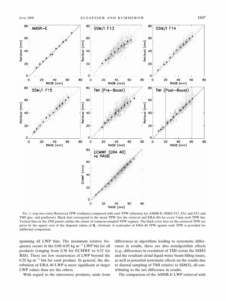
A scatterplot of the retrieved TPW against radio-sonde-observed (raob) TPW is shown in Fig. 1 for allsensors used in this study. ERA-40 TPW plottedagainst raob TPW is shown for additional comparison.The results for the surface wind speed retrieval areshown in Fig. 2. The black error bars (square root of thediagonal values of Sx) show the one-sigma standard de-viation errors on the retrieved TPW. As was discussed,optimal estimation provides an error for each elementof the retrieved state vector. For plotting purposes, datawere binned, and the mean retrieval error was plottedfor each bin containing more than 40 pixel matchups(5-mm bin size for TPW; 1 m s�1 bin size for WIND).

From a qualitative inspection of Fig. 1, one can seethat the scatter within the retrieved TPW dataset con-tributing to the total root-mean square (RMS) error farexceeds the optimal estimation retrieval error. This isnot the case with the surface wind retrieval, as seen inFig. 2. One possible reason for this is related to thecoincident matchup requirements. As was mentioned,since the requirements for matching retrieved TPW toraob TPW are much less restrictive than they are forsurface wind retrieval matchups, and because this is notaccounted for in the calculation of Sx, this could lead toadditional RMS error when comparing the TPW re-trieval with in situ raob TPW.

Table 2 gives a breakdown of the statistics (meanbias, unadjusted RMS error) corresponding to the TPWand WIND retrievals for all five sensors used in thisstudy. The number of in situ collocations for each sen-sor matchup is also provided in Table 2. As can be seen,for both TPW and WIND, biases (retrieved � ob-served) of differing magnitudes were found for eachsensor.

For TPW, biases range from �0.04 mm (for TMIpreboost) to �2.78 mm (SSM/I F15). Additionally,RMS errors range from 2.99 mm (AMSR-E) to 5.93mm (SSM/I F13). ERA-40 TPW is in good agreement

with raob TPW with a mean bias of �1.35 mm and anRMS error of 3.61 mm. It should be noted that ERA-40assimilates these raobs and, thus, the good agreement isnot very surprising. The retrieval error statistics are inreasonable comparison to other microwave algorithmsavailable. Jackson and Stephens (1995) performed analgorithm intercomparison for TPW retrievals usingSSM/I F08 and found RMS errors (relative to raobs)ranging from 4.66 mm [Alishouse et al. (1990) statisticalalgorithm] to 5.08 mm [Greenwald et al. (1995) physicalalgorithm], with biases in some algorithms approaching1 mm. Vertical lines have been added to the TMI pre-boost and postboost panels to highlight that some of thediscrepancies that exist when visually comparing thetwo periods arise from the fact that the very low TPWregimes are not sampled during the preboost periodand the very high TPW regimes are not sampled duringthe postboost period. This is partly the cause for differ-ences in the mean TPW bias between the two periods.Because raob overpass locations are not the same be-tween the two periods, different regimes may besampled and model bias may be making itself known.Aside from these issues, the cause of the additionaldiscrepancy between the two periods is not known atthis time.

For WIND, biases range from �0.64 m s�1 (for TMIpostboost) to �1.73 m s�1 (SSM/I F14). RMS errorsrange from 1.40 m s�1 (TMI postboost) to 1.87 m s�1

(SSM/I F13 and F14). Additionally, ERA-40 comparesreasonably well to the in situ data with a mean windspeed bias of �0.62 m s�1 and RMS error of 1.62 m s�1.The retrieval errors are also comparable to the 1.52m s�1 RMS error for a retrieval of TMI surface windspeed (compared to buoy) found by Connor and Chang(2000). Furthermore, Chang and Li (1998) used the op-erational Goodberlet and Swift (1992) surface windspeed retrieval algorithm for SSM/I F11 and found anRMS error of approximately 2.3 m s�1. Quantificationof the magnitudes and directions of the wind speedbiases were not available in either study.

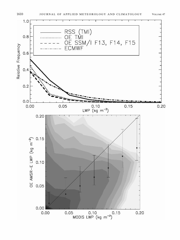
The LWP retrieval results for SSM/I and TMI areshown in the top panel of Fig. 3. For these sensors, thecomparison is limited to both ERA-40 and an indepen-dent microwave retrieval algorithm used by RSS. TheERA-40 LWP global dataset is a 2.5° � 2.5° daily grid-ded product. In this study, since the LWP retrieval iscomputed at pixel resolution, the pixel-level LWP val-ues are averaged to the same 2.5° � 2.5° resolution formore appropriate comparison. RSS LWP retrievals aretreated in the same manner. The relative frequency (yaxis) of a particular LWP is derived by computing thenumber of LWP occurrences in an LWP bin of arbitrarysize and dividing by the total number of occurrences


spanning all LWP bins. The maximum relative fre-quency occurs in the 0.00–0.05 kg m�2 LWP bin for allproducts (ranging from 0.38 for ECMWF to 0.52 forRSS). There are few occurrences of LWP beyond the0.20 kg m�2 bin for each product. In general, the dis-tribution of ERA-40 LWP is more significant at largerLWP values than are the others.

With regard to the microwave products, aside from

differences in algorithms leading to systematic differ-ences in results, there are also nonalgorithm effects(e.g., differences in resolution of TMI versus the SSM/Iand the resultant cloud liquid water beam-filling issues,as well as potential systematic effects on the results dueto diurnal sampling of TMI relative to SSM/I), all con-tributing to the net difference in results.

The comparison of the AMSR-E LWP retrieval with

FIG. 1. (top two rows) Retrieved TPW (ordinate) compared with raob TPW (abscissa) for AMSR-E; SSM/I F13, F14, and F15; andTMI (pre- and postboost). Black dots correspond to the mean TPW (for the retrieval and ERA-40) for every 5-mm raob TPW bin.Vertical lines in the TMI panels outline the extent of common-sampled TPW regimes. The black error bars on the retrieved TPW aregiven by the square root of the diagonal values of Sx. (bottom) A scatterplot of ERA-40 TPW against raob TPW is provided foradditional comparison.


the optical LWP estimate is shown in the bottom panelof Fig. 3. Data were binned and the mean retrieval andone-sigma retrieval error (black error bars) were plot-ted for each bin containing more than 40 pixel match-ups (approximately a 0.03–0.04 kg m�2 bin size). Con-tours represent relative data densities and are chosen atarbitrary intervals. Optical estimates for LWP can bederived using cloud optical thickness and cloud dropleteffective radius (Bennartz 2007; Horvath and Davies

2007; Lin and Rossow 1994). These two parameters canbe retrieved from simultaneous solar reflectance mea-surements at a nonabsorbing visible and a water-absorbing near-infrared channel (Nakajima and King,1990), both of which are available from the MODISinstrument. The errors associated with the optical tech-nique can be found in King et al. (1997).

The microwave and optical techniques represent dif-ferent, independent approaches for retrieving LWP

FIG. 2. (top two rows) Retrieved WIND (ordinate) compared with buoy WIND (abscissa) for AMSR-E; SSM/I F13, F14, and F15;and TMI (pre- and postboost) and (bottom) a scatterplot of ERA-40 WIND vs buoy WIND. Black dots correspond to the mean WIND(for the retrieval and ERA-40) for every 1 m s�1 buoy WIND bin. The black error bars on the retrieved WIND are given by the squareroot of the diagonal values of Sx.


from space. The mean LWPs from AMSR-E andMODIS are both approximately 0.04 kg m�2, with themicrowave retrieval slightly overestimating (�0.002 kgm�2) the optical retrieval in a mean sense. It wouldappear that the AMSR-E mean LWP should be notice-ably lower than the optical mean LWP. However, wepoint out that the bias in LWP is a function of locationin LWP space (i.e., microwave technique overestimatesat the lowest LWPs while the optical technique over-estimates beyond the 0.02 kg m�2 LWP threshold). Thecompeting effects between the high bias at the low endwhere much more data are available and the low bias athigher LWPs (data much more sparse) contribute tothe two means being approximately the same.

Lin and Rossow (1994) also found that in an averagesense, microwave and optical estimates of LWP agreewell (both having a mean of 0.05 kg m�2) for overcast,warm, nonprecipitating clouds in calm sea environ-ments, generally in agreement with our findings. Ben-nartz (2007), in studying boundary layer clouds in theSouth Pacific Ocean off the South American coast alsofound that while the average LWP is in agreement be-tween the two estimates, the microwave algorithm con-sistently overestimates at low LWP values and under-estimates at higher LWP values. The low sensitivity ofthe microwave technique to very low values of LWPmakes it difficult for the microwave retrieval to distin-guish between clear and cloudy scenes (Lin and Rossow1994), adding to the error in the microwave retrieval.Horvath and Davies (2007) note that the MODIS cloudmask may have missed a number of the shallow cumu-lus cloud fields, therefore causing an underestimationin the subdomain cloud fraction, in turn resulting in anunderestimation of the average LWP over the domain(and possibly explaining some of the high bias at thelow end of the LWP spectrum). Bennartz (2007) notesthat the reason for the low bias at higher LWPs is un-clear. However, since the field of view for AMSR-E ismuch larger than the field of view for MODIS, beam-filling effects due to the nonlinear relationship between

LWP and brightness temperature in conjunction withthe larger AMSR-E footprint and likely inhomogene-ities in the cloud field over the larger AMSR-E foot-print are likely to lead to an underestimation in themicrowave LWP (Bennartz 2007) when comparing thetwo products. Additionally, rain contamination can bean issue as well (Bennartz 2007), since the absorption/emission signal for lightly raining clouds (no ice) is simi-lar to that of nonprecipitating, cloud water-only systems.

5. Additional applications

a. Rainfall detection

The algorithm developed for this study contains thenecessary physics to model the propagation of micro-wave radiation through nonprecipitating scenes inwhich absorption and emission are the only radiativetransfer processes present. As such, the application ofthis algorithm over raining scenes for which scatteringof microwave radiation must be taken into account willresult in simulated brightness temperatures that do notagree with the observations. Therefore, �2 will be con-sistently larger in magnitude than expected in such in-stances. The differences between simulated and ob-served brightness temperatures continue to increasewith increasing rain rate as the scattering signature atthe higher-frequency channels along with the emissionsignature at the lowest-frequency channels becomemore evident and the retrieval has greater difficulty infinding a solution that yields brightness temperaturesthat agree with the observations. The relationship,then, between the increased contribution to the costfunction (a higher �2) and increasing rain rates is ex-pected to be consistent and can be used to identifyscenes for which rainfall is occurring. The unique re-sponse of the optimal estimation �2 parameter to theradiometric signatures associated with raining systemsallows for the development of a rainfall detectionscheme to be used in either the rain–no-rain determi-nation aspect of rainfall retrieval or as a screen to in-

TABLE 2. TPW and WIND retrieval performance for AMSR-E; SSM/I F13, F14, and F15; and TMI. Integrated water vapor andsurface wind speed from ERA-40 in comparison with in situ results are shown for additional comparison.

Sensor

TPW WIND

Collocations Bias (mm) RMS error (mm) Collocations Bias (m s�1) RMS error (m s�1)

AMSR-E 669 �0.99 2.99 22979 �1.05 1.45SSM/I F13 4225 �0.26 5.93 15381 �1.26 1.87SSM/I F14 1906 �2.29 4.28 15430 �1.73 1.87SSM/I F15 2096 �2.78 4.43 13148 �1.00 1.84TMI preboost 6170 �0.04 5.15 66111 �0.82 1.50TMI postboost 4478 �1.00 4.53 44054 �0.64 1.40ECMWF 4885 �1.35 3.61 62647 �0.62 1.62


ternally filter out regions contaminated by rainfall incloud property retrieval. The viability of this applica-tion is discussed below.

CASE STUDIES

The consistent response to radiances upwelling fromraining systems in �2 provides for a new capability inrainfall detection. Using information from the 2A25product, the expected response of �2 to rainfall can beevaluated. The TRMM PR swath generally follows atrack collocated with the center pixels of the TMIswath. The black lines extending across the center ofthe TMI swaths in Figs. 4–6 outline the extent of theTRMM PR swath. While the purpose of this study isnot to choose and advocate for a diagnostic thresholdbelow (beyond) which the scene is considered nonrain-ing (raining), for the purpose of illustrating and visual-izing the consistent response of the �2 to rainfall, athreshold is chosen so areas that exceed the currently

considered operational threshold are masked out andevaluated against the corresponding 2A25 near-surfacerain rates. These masked regions are those for whichthe possibility of precipitation exists. Only regions lyingwithin the TRMM PR swath are blacked out. For thispaper, the possibility of precipitation based on a �2

threshold occurs when �2 � 40.0. This �2 value for rain–no-rain discrimination is chosen using the 2A25 productas the basis for the determination of rain (approxi-mately 0.1 mm h�1 rain rate threshold) and was ob-tained by computing the average minimum value of �2

when the 2A25 product indicates rainfall over the pe-riod from January to December 2000 (during the pre-boost period of TRMM).

(i) Raining scenes

Figure 4 shows two scenes for which the 2A25 prod-uct indicated precipitation. The blacked-out regions inthe �2 panels of Fig. 4 agree fairly well with the areas of

←

FIG. 3. (top) Relative frequency of retrieved nonprecipitating LWP occurrences from the optimal estimation (OE) algorithm, RSS,and the ERA-40 dataset. Data are averaged into 2.5° � 2.5° grid boxes spanning 40°S–40°N and 180°W–180°E for comparison withERA-40. (bottom) Comparison of the AMSR-E LWP retrieval with the optical LWP estimates from MODIS. Data were binned andthe mean retrieval (black dots) and one-sigma retrieval error (black error bars) was plotted for each bin containing more than 40 pixels.Contours represent relative data densities and are chosen at arbitrary intervals for visual purposes.

FIG. 4. TRMM orbit snapshots of raining scenes (according to TRMM PR) over the Pacific Ocean on (top left)1 Feb 2000 and (top right) 27 Aug 2004. The corresponding optimal estimation �2 diagnostic can be seen in thebottom panels. Regions blacked out in the �2 panels contain those satellite pixels considered to be rainingaccording to the no-rain thresholds currently being considered for operational use.


Fig 4 live 4/C

precipitation according to 2A25. As expected, theagreement is best for those areas with higher rain rates(e.g., 2A25 rain rates exceeding �1 mm h�1). Thesescenes are unable to be explained by emission/absorp-

tion only and thus the simulated brightness tempera-tures do not agree with the observations, as indicatedby values that exceed the currently considered thresh-old for �2. These scenes illustrate the potential of the

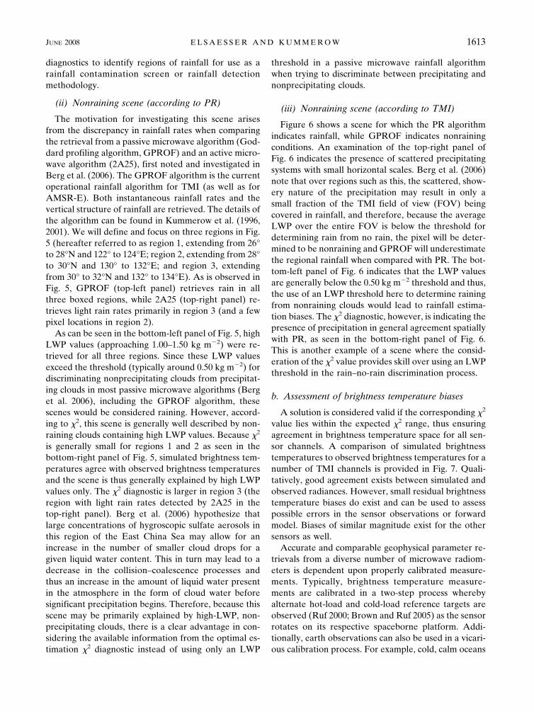
FIG. 6. (top right) An orbit snapshot on 1 Feb 2000 for which TRMM PR indicates rainfall. (top left) No rainfallwas retrieved using the GPROF algorithm. The associated LWP and �2 can be seen in the bottom two panels.

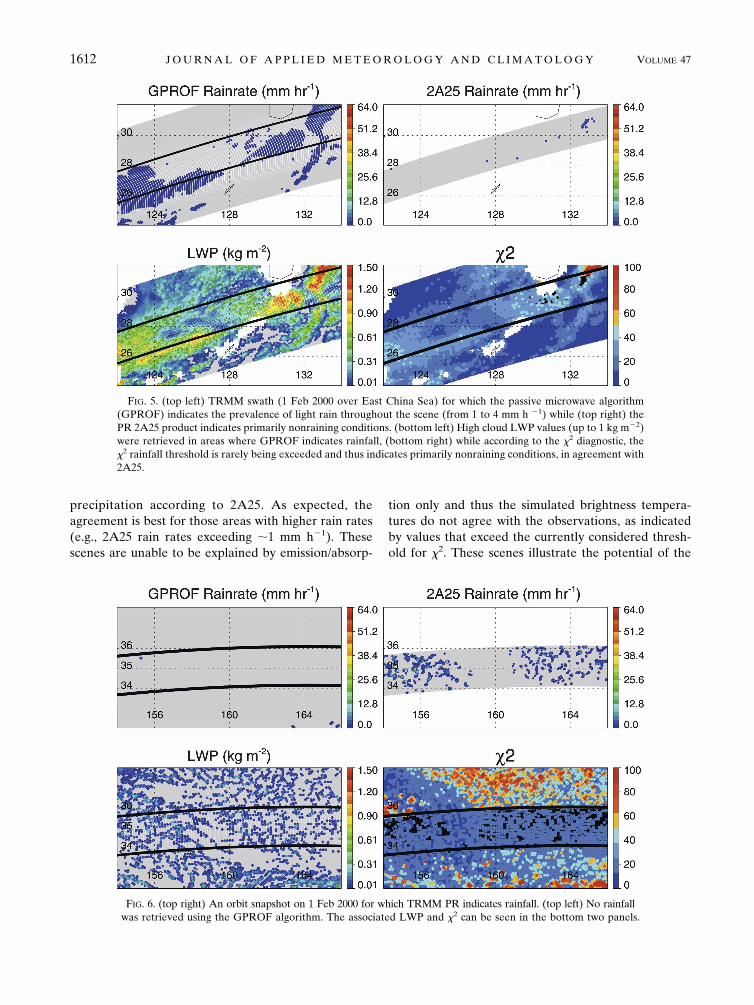
FIG. 5. (top left) TRMM swath (1 Feb 2000 over East China Sea) for which the passive microwave algorithm(GPROF) indicates the prevalence of light rain throughout the scene (from 1 to 4 mm h �1) while (top right) thePR 2A25 product indicates primarily nonraining conditions. (bottom left) High cloud LWP values (up to 1 kg m�2)were retrieved in areas where GPROF indicates rainfall, (bottom right) while according to the �2 diagnostic, the�2 rainfall threshold is rarely being exceeded and thus indicates primarily nonraining conditions, in agreement with2A25.


Fig 5 6 live 4/C

diagnostics to identify regions of rainfall for use as arainfall contamination screen or rainfall detectionmethodology.

(ii) Nonraining scene (according to PR)

The motivation for investigating this scene arisesfrom the discrepancy in rainfall rates when comparingthe retrieval from a passive microwave algorithm (God-dard profiling algorithm, GPROF) and an active micro-wave algorithm (2A25), first noted and investigated inBerg et al. (2006). The GPROF algorithm is the currentoperational rainfall algorithm for TMI (as well as forAMSR-E). Both instantaneous rainfall rates and thevertical structure of rainfall are retrieved. The details ofthe algorithm can be found in Kummerow et al. (1996,2001). We will define and focus on three regions in Fig.5 (hereafter referred to as region 1, extending from 26°to 28°N and 122° to 124°E; region 2, extending from 28°to 30°N and 130° to 132°E; and region 3, extendingfrom 30° to 32°N and 132° to 134°E). As is observed inFig. 5, GPROF (top-left panel) retrieves rain in allthree boxed regions, while 2A25 (top-right panel) re-trieves light rain rates primarily in region 3 (and a fewpixel locations in region 2).

As can be seen in the bottom-left panel of Fig. 5, highLWP values (approaching 1.00–1.50 kg m�2) were re-trieved for all three regions. Since these LWP valuesexceed the threshold (typically around 0.50 kg m�2) fordiscriminating nonprecipitating clouds from precipitat-ing clouds in most passive microwave algorithms (Berget al. 2006), including the GPROF algorithm, thesescenes would be considered raining. However, accord-ing to �2, this scene is generally well described by non-raining clouds containing high LWP values. Because �2

is generally small for regions 1 and 2 as seen in thebottom-right panel of Fig. 5, simulated brightness tem-peratures agree with observed brightness temperaturesand the scene is thus generally explained by high LWPvalues only. The �2 diagnostic is larger in region 3 (theregion with light rain rates detected by 2A25 in thetop-right panel). Berg et al. (2006) hypothesize thatlarge concentrations of hygroscopic sulfate aerosols inthis region of the East China Sea may allow for anincrease in the number of smaller cloud drops for agiven liquid water content. This in turn may lead to adecrease in the collision–coalescence processes andthus an increase in the amount of liquid water presentin the atmosphere in the form of cloud water beforesignificant precipitation begins. Therefore, because thisscene may be primarily explained by high-LWP, non-precipitating clouds, there is a clear advantage in con-sidering the available information from the optimal es-timation �2 diagnostic instead of using only an LWP

threshold in a passive microwave rainfall algorithmwhen trying to discriminate between precipitating andnonprecipitating clouds.

(iii) Nonraining scene (according to TMI)

Figure 6 shows a scene for which the PR algorithmindicates rainfall, while GPROF indicates nonrainingconditions. An examination of the top-right panel ofFig. 6 indicates the presence of scattered precipitatingsystems with small horizontal scales. Berg et al. (2006)note that over regions such as this, the scattered, show-ery nature of the precipitation may result in only asmall fraction of the TMI field of view (FOV) beingcovered in rainfall, and therefore, because the averageLWP over the entire FOV is below the threshold fordetermining rain from no rain, the pixel will be deter-mined to be nonraining and GPROF will underestimatethe regional rainfall when compared with PR. The bot-tom-left panel of Fig. 6 indicates that the LWP valuesare generally below the 0.50 kg m�2 threshold and thus,the use of an LWP threshold here to determine rainingfrom nonraining clouds would lead to rainfall estima-tion biases. The �2 diagnostic, however, is indicating thepresence of precipitation in general agreement spatiallywith PR, as seen in the bottom-right panel of Fig. 6.This is another example of a scene where the consid-eration of the �2 value provides skill over using an LWPthreshold in the rain–no-rain discrimination process.

b. Assessment of brightness temperature biases

A solution is considered valid if the corresponding �2

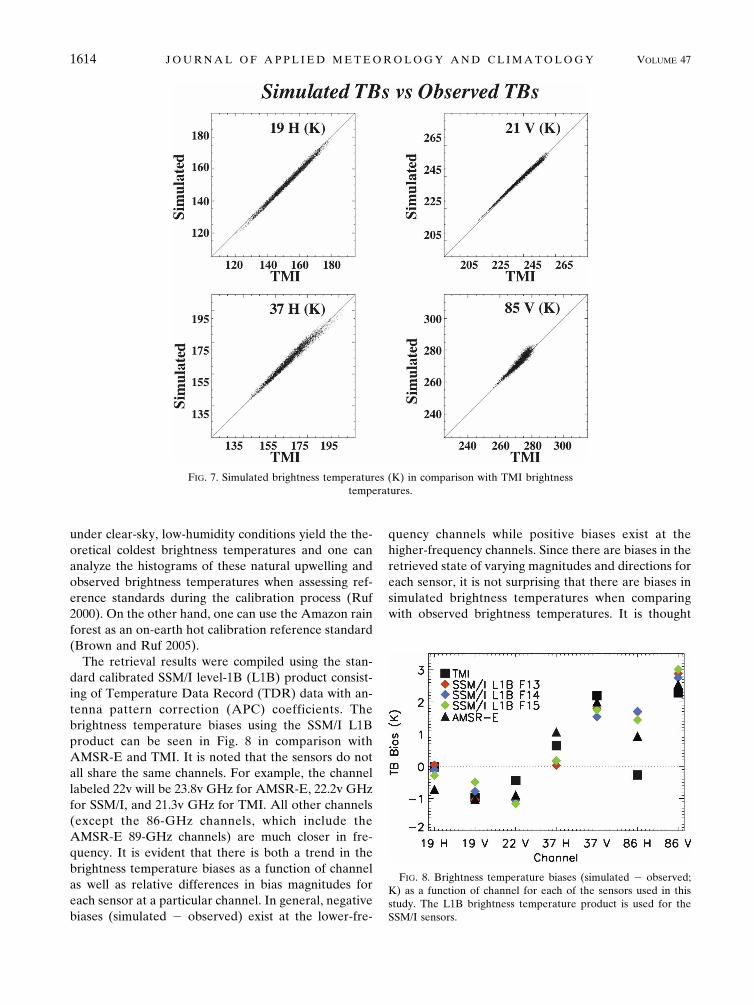
value lies within the expected �2 range, thus ensuringagreement in brightness temperature space for all sen-sor channels. A comparison of simulated brightnesstemperatures to observed brightness temperatures for anumber of TMI channels is provided in Fig. 7. Quali-tatively, good agreement exists between simulated andobserved radiances. However, small residual brightnesstemperature biases do exist and can be used to assesspossible errors in the sensor observations or forwardmodel. Biases of similar magnitude exist for the othersensors as well.

Accurate and comparable geophysical parameter re-trievals from a diverse number of microwave radiom-eters is dependent upon properly calibrated measure-ments. Typically, brightness temperature measure-ments are calibrated in a two-step process wherebyalternate hot-load and cold-load reference targets areobserved (Ruf 2000; Brown and Ruf 2005) as the sensorrotates on its respective spaceborne platform. Addi-tionally, earth observations can also be used in a vicari-ous calibration process. For example, cold, calm oceans


under clear-sky, low-humidity conditions yield the the-oretical coldest brightness temperatures and one cananalyze the histograms of these natural upwelling andobserved brightness temperatures when assessing ref-erence standards during the calibration process (Ruf2000). On the other hand, one can use the Amazon rainforest as an on-earth hot calibration reference standard(Brown and Ruf 2005).

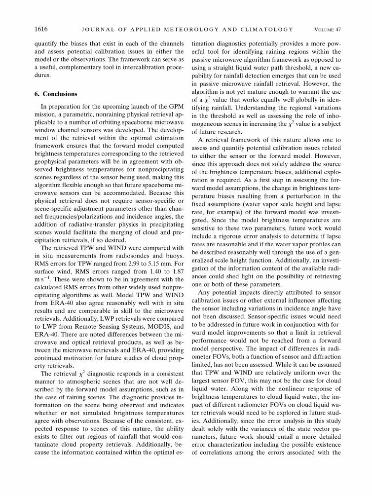
The retrieval results were compiled using the stan-dard calibrated SSM/I level-1B (L1B) product consist-ing of Temperature Data Record (TDR) data with an-tenna pattern correction (APC) coefficients. Thebrightness temperature biases using the SSM/I L1Bproduct can be seen in Fig. 8 in comparison withAMSR-E and TMI. It is noted that the sensors do notall share the same channels. For example, the channellabeled 22v will be 23.8v GHz for AMSR-E, 22.2v GHzfor SSM/I, and 21.3v GHz for TMI. All other channels(except the 86-GHz channels, which include theAMSR-E 89-GHz channels) are much closer in fre-quency. It is evident that there is both a trend in thebrightness temperature biases as a function of channelas well as relative differences in bias magnitudes foreach sensor at a particular channel. In general, negativebiases (simulated � observed) exist at the lower-fre-

quency channels while positive biases exist at thehigher-frequency channels. Since there are biases in theretrieved state of varying magnitudes and directions foreach sensor, it is not surprising that there are biases insimulated brightness temperatures when comparingwith observed brightness temperatures. It is thought

FIG. 8. Brightness temperature biases (simulated � observed;K) as a function of channel for each of the sensors used in thisstudy. The L1B brightness temperature product is used for theSSM/I sensors.

FIG. 7. Simulated brightness temperatures (K) in comparison with TMI brightnesstemperatures.


Fig 8 live 4/C

that the relative differences in brightness temperaturebiases for a particular channel are more representativeof effects that arise due to the sensor being used [e.g.,systematic measurement error could arise from issuesrelated to the calibration system on the sensor (warm-load temperature and emissivity), reflector emissivity,or antenna pattern correction errors] while the generaltrend as a function of channel is more representative ofthe forward model bias.

For this study, an intercalibrated brightness tempera-ture product is also utilized. This product containsSSM/I brightness temperatures calibrated to TMI [com-mon calibrated brightness temperature product, alsoknown as the level-1C (L1C) product; informationavailable online at http://rain.atmos.colostate.edu] us-ing a reference geophysical parameter dataset fromRSS to simulate brightness temperatures. This datasetwas derived with the goal of ensuring consistencyamong microwave products generated using differentsensors in preparation for GPM. The geophysical pa-rameter results for this study are based on the SSM/IL1C intercalibrated brightness temperature product.The magnitudes and directions of the biases for similarmicrowave channels for each of the sensors (now usingthe L1C product for SSM/I) are shown in Fig. 9. Prigentet al. (1997) found systematic differences in the samedirection and of similar magnitude for the SSM/I in-strument on board DMSP satellites F11 and F13.Karstens et al. (1994) also found biases following achannel-dependent trend similar to that of this studyduring the International Cirrus Experiment (ICE’89)for SSM/I on board DMSP F08 for all channels (notusing 85 GHz) when comparing observed brightnesstemperatures to simulated brightness temperatures de-

rived using raob and synoptic observations. In thatstudy, however, biases were of much larger magnituderanging from �2.7 to �3.3 K for frequencies less than22 GHz and from �1.5 K to �2.0 K for the 37-GHzchannels.

One can see from a comparison of the brightnesstemperature biases using the SSM/I L1B products (Fig.8) with the SSM/I intercalibrated L1C product usingTMI as a reference standard (Fig. 9) that the resultantmean SSM/I brightness temperature biases using theL1C product are relatively similar to TMI in magnitudeand direction; this is particularly evident in the higher-frequency channels. These results are consistent withthe L1C efforts. It is noted that AMSR-E is currentlynot calibrated to TMI, despite the AMSR-E brightnesstemperature biases being similar to the other sensorbiases.

By modifying a number of forward model assump-tions, the impact on the general brightness temperaturebias trend over all channels can be investigated. Forexample, if the water vapor scale height and tempera-ture lapse rate are fixed (2.0 km and 6.0 K km�1, re-spectively) globally as opposed to using ERA-40 infor-mation, one will note that the general trend of thebrightness temperature biases changes while the rela-tive differences between sensors at particular channelsremain generally fixed, as can be seen when comparingFigs. 9 and 10. For example, the “group” of biases as awhole changes drastically, which is particularly evidentin the 86-GHz channels, while the relative differencesremain approximately constant.

The nature of the optimal estimation framework al-lows one to assess the differences between simulatedand observed radiances after the geophysical parametersolution has been found. Thus, it becomes possible to

FIG. 9. As in Fig. 8 but for the SSM/I level-1C intercalibratedbrightness temperature product. These brightness temperature bi-ases are the ones that correspond to the geophysical parameterretrieval results in section 4.

FIG. 10. As in Fig. 9 but for a recompilation of the results usingmodified forward model assumptions (new water vapor scaleheight and temperature lapse rate).


Fig 9 10 live 4/C

quantify the biases that exist in each of the channelsand assess potential calibration issues in either themodel or the observations. The framework can serve asa useful, complementary tool in intercalibration proce-dures.

6. Conclusions

In preparation for the upcoming launch of the GPMmission, a parametric, nonraining physical retrieval ap-plicable to a number of orbiting spaceborne microwavewindow channel sensors was developed. The develop-ment of the retrieval within the optimal estimationframework ensures that the forward model computedbrightness temperatures corresponding to the retrievedgeophysical parameters will be in agreement with ob-served brightness temperatures for nonprecipitatingscenes regardless of the sensor being used, making thisalgorithm flexible enough so that future spaceborne mi-crowave sensors can be accommodated. Because thisphysical retrieval does not require sensor-specific orscene-specific adjustment parameters other than chan-nel frequencies/polarizations and incidence angles, theaddition of radiative-transfer physics in precipitatingscenes would facilitate the merging of cloud and pre-cipitation retrievals, if so desired.

The retrieved TPW and WIND were compared within situ measurements from radiosondes and buoys.RMS errors for TPW ranged from 2.99 to 5.15 mm. Forsurface wind, RMS errors ranged from 1.40 to 1.87m s�1. These were shown to be in agreement with thecalculated RMS errors from other widely used nonpre-cipitating algorithms as well. Model TPW and WINDfrom ERA-40 also agree reasonably well with in situresults and are comparable in skill to the microwaveretrievals. Additionally, LWP retrievals were comparedto LWP from Remote Sensing Systems, MODIS, andERA-40. There are noted differences between the mi-crowave and optical retrieval products, as well as be-tween the microwave retrievals and ERA-40, providingcontinued motivation for future studies of cloud prop-erty retrievals.

The retrieval �2 diagnostic responds in a consistentmanner to atmospheric scenes that are not well de-scribed by the forward model assumptions, such as inthe case of raining scenes. The diagnostic provides in-formation on the scene being observed and indicateswhether or not simulated brightness temperaturesagree with observations. Because of the consistent, ex-pected response to scenes of this nature, the abilityexists to filter out regions of rainfall that would con-taminate cloud property retrievals. Additionally, be-cause the information contained within the optimal es-

timation diagnostics potentially provides a more pow-erful tool for identifying raining regions within thepassive microwave algorithm framework as opposed tousing a straight liquid water path threshold, a new ca-pability for rainfall detection emerges that can be usedin passive microwave rainfall retrieval. However, thealgorithm is not yet mature enough to warrant the useof a �2 value that works equally well globally in iden-tifying rainfall. Understanding the regional variationsin the threshold as well as assessing the role of inho-mogeneous scenes in increasing the �2 value is a subjectof future research.

A retrieval framework of this nature allows one toassess and quantify potential calibration issues relatedto either the sensor or the forward model. However,since this approach does not solely address the sourceof the brightness temperature biases, additional explo-ration is required. As a first step in assessing the for-ward model assumptions, the change in brightness tem-perature biases resulting from a perturbation in thefixed assumptions (water vapor scale height and lapserate, for example) of the forward model was investi-gated. Since the model brightness temperatures aresensitive to these two parameters, future work wouldinclude a rigorous error analysis to determine if lapserates are reasonable and if the water vapor profiles canbe described reasonably well through the use of a gen-eralized scale height function. Additionally, an investi-gation of the information content of the available radi-ances could shed light on the possibility of retrievingone or both of these parameters.

Any potential impacts directly attributed to sensorcalibration issues or other external influences affectingthe sensor including variations in incidence angle havenot been discussed. Sensor-specific issues would needto be addressed in future work in conjunction with for-ward model improvements so that a limit in retrievalperformance would not be reached from a forwardmodel perspective. The impact of differences in radi-ometer FOVs, both a function of sensor and diffractionlimited, has not been assessed. While it can be assumedthat TPW and WIND are relatively uniform over thelargest sensor FOV, this may not be the case for cloudliquid water. Along with the nonlinear response ofbrightness temperatures to cloud liquid water, the im-pact of different radiometer FOVs on cloud liquid wa-ter retrievals would need to be explored in future stud-ies. Additionally, since the error analysis in this studydealt solely with the variances of the state vector pa-rameters, future work should entail a more detailederror characterization including the possible existenceof correlations among the errors associated with the


retrieved parameters, as well as their possible regimedependence.

Acknowledgments. ECMWF ERA-40 data used inthis study have been obtained from the ECMWF dataserver. AMSR-E sea surface temperatures and TMIliquid water paths are produced by Remote SensingSystems and sponsored by the NASA Earth ScienceREASoN DISCOVER Project. Data are available on-line (at www.remss.com). MODIS data were obtainedfrom the NASA Goddard Distributed Active ArchiveCenter. This research was supported by NASA GrantNAG5-13694.

REFERENCES

Alishouse, J. C., S. A. Snyder, J. Vongsathorn, and R. R. Ferraro,1990: Determination of oceanic total precipitable water fromthe SSM/I. IEEE Trans. Geosci. Remote Sens., 28, 811–816.

Bennartz, R., 2007: Global assessment of marine boundary layercloud droplet number concentration from satellite. J. Geo-phys. Res., 112, D02201, doi:10.1029/2006JD007547.

Berg, W., T. L’Ecuyer, and C. Kummerow, 2006: Rainfall climateregimes: The relationship of regional TRMM rainfall biasesto the environment. J. Appl. Meteor., 45, 434–454.

Brown, S. T., and C. S. Ruf, 2005: Determination of an Amazonhot reference target for the on-orbit calibration of microwaveradiometers. J. Atmos. Oceanic Technol., 22, 1340–1352.

Chang, P. S., and L. Li, 1998: Ocean surface wind speed and di-rection retrievals from the SSM/I. IEEE Trans. Geosci. Re-mote Sens., 36, 1866–1871.

Colton, M. C., and G. A. Poe, 1999: Intersensor calibration ofDMSP SSM/I’s: F-8 to F-14, 1987–1997. IEEE Trans. Geosci.Remote Sens., 37, 418–439.

Connor, L. N., and P. S. Chang, 2000: Ocean surface wind retriev-als using the TRMM Microwave Imager. IEEE Trans.Geosci. Remote Sens., 38, 2009–2016.

Deblonde, G., and S. J. English, 2001: Evaluation of theFASTEM-2 fast microwave ocean surface emissivity model.Tech. Proc. Int. TOVS Study Conf. XI, Budapest, Hungary,WMO, 67–78.

Durre, I., R. S. Vose, and D. B. Wuertz, 2006: Overview of theIntegrated Global Radiosonde Archive. J. Climate, 19, 53–67.

Ferraro, R. R., E. A. Smith, W. Berg, and G. J. Huffman, 1998: Ascreening methodology for passive microwave precipitationretrieval algorithms. J. Atmos. Sci., 55, 1583–1600.

Foster, J., M. Bevis, and W. Raymond, 2006: Precipitable waterand the lognormal distribution. J. Geophys. Res., 111,D15102, doi:10.1029/2005JD006731.

Goodberlet, M. A., and C. T. Swift, 1992: Improved retrieval fromthe DMSP wind speed algorithm under adverse weather con-ditions. IEEE Trans. Geosci. Remote Sens., 30, 1076–1077.

Greenwald, T. J., G. L. Stephens, S. A. Christopher, and T. H.Vonder Haar, 1995: Observations of the global characteristicsand regional radiative effects of marine cloud liquid water. J.Climate, 8, 2928–2946.

Hollinger, J. P., R. Lo, and G. Poe, 1987: Special Sensor Micro-wave/Imager user’s guide. NRL Tech. Rep. 579269, 120 pp.[Available from Naval Research Laboratory, Washington,DC 20375-5337.]

——, J. L. Peirce, and G. A. Poe, 1990: SSM/I instrument evalu-ation. IEEE Trans. Geosci. Remote Sens., 28, 781–790.

Horvath, A., and R. Davies, 2007: Comparison of microwave andoptical cloud water path estimates from TMI, MODIS, andMISR. J. Geophys. Res., 112, D01202, doi:10.1029/2006JD007101.

Huang, H.-L., and G. R. Diak, 1992: Retrieval of nonprecipitatingliquid water cloud parameters from microwave data: A simu-lation study. J. Atmos. Oceanic Technol., 9, 354–363.

Iguchi, T., T. Kozu, R. Meneghini, J. Awaka, and K. Okamoto,2000: Rain-profiling algorithm for the TRMM precipitationradar. J. Appl. Meteor., 39, 2038–2052.

Isaacs, R. G., and G. Deblonde, 1987: Millimeter wave moisturesounding: The effect of clouds. Radio Sci., 22, 367–377.

Jackson, D. L., and G. L. Stephens, 1995: A study of SSM/I-derived columnar water vapor over the global oceans. J. Cli-mate, 8, 2025–2038.

Karstens, U., C. Simmer, and E. Ruprecht, 1994: Remote sensingof cloud liquid water. Meteor. Atmos. Phys., 54, 157–171.

Kawanishi, T., and Coauthors, 2003: The Advanced MicrowaveScanning Radiometer for the Earth Observing System(AMSR-E): NASDA’s contribution to the EOS for GlobalEnergy and Water Cycle Studies. IEEE Trans. Geosci. Re-mote Sens., 41, 184–194.

King, M. D., S.-C. Tsay, S. E. Platnick, M. Wang, and K.-N. Liou,1997: Cloud retrieval algorithms for MODIS: Optical thick-ness, effective particle radius, and thermodynamic phase.MODIS Algorithm Theoretical Basis Doc. ATBD-MOD-05,Version 5, NASA Goddard Space Flight Center, Greenbelt,MD, 79 pp. [Available online at http://modis-atmos.gsfc.nasa.gov/_docs/atbd_mod05.pdf.]

Kohn, D. J., 1995: Refinement of a semi-empirical model for themicrowave emissivity of the sea surface as a function of windspeed. M.S. thesis, Dept. of Meteorology, Texas A&M Uni-versity, 44 pp.

Kummerow, C., W. S. Olson, and L. Giglio, 1996: A simplifiedscheme for obtaining precipitation and vertical hydrometeorprofiles from passive microwave sensors. IEEE Trans.Geosci. Remote Sens., 34, 1213–1232.

——, W. Barnes, T. Kozu, J. Shiue, and J. Simpson, 1998: TheTropical Rainfall Measuring Mission (TRMM) sensor pack-age. J. Atmos. Oceanic Technol., 15, 809–817.

——, and Coauthors, 2001: The evolution of the Goddard Profil-ing Algorithm (GPROF) for rainfall estimation from passivemicrowave sensors. J. Appl. Meteor., 40, 1801–1820.

——, W. Berg, J. Thomas-Stahle, and H. Masunaga, 2006: Quan-tifying global uncertainties in a simple microwave rainfallalgorithm. J. Atmos. Oceanic Technol., 23, 23–37.

Liebe, H. J., G. A. Hufford, and T. Manabe, 1991: A model for thecomplex permittivity of water at frequencies below 1 THz.Int. J. Infrared Millimeter Waves, 12, 659–675.

——, ——, and M. G. Cotton, 1993: Propagation modeling ofmoist air and suspended water particles at frequencies below1000 GHz. Advisory Group for Aerospace Research and De-velopment Conf. Proc: Atmospheric Propagation Effectsthrough Natural and Man-Made Obscurants for Visible toMM-Wave Radiation (AGARD-CP-542), AGARD, Neuillysur Seine, France, 3-1–3-10.

Liljegren, J. C., S. A. Boukabara, K. Cady-Pereira, and S. A.Clough, 2005: The effect of the half-width of the 22-GHzwater vapor line on retrievals of temperature and water va-por profiles with a 12-channel microwave radiometer. IEEETrans. Geosci. Remote Sens., 43, 1102–1108.


Lin, B., and W. A. Rossow, 1994: Observations of cloud liquidwater path over oceans: Optical and microwave remote sens-ing methods. J. Geophys. Res., 99, 20 907–20 927.

Liu, G., and J. A. Curry, 1993: Determination of characteristicfeatures of cloud liquid water from satellite microwave mea-surements. J. Geophys. Res., 98, 5069–5092.

Marks, C. J., and C. D. Rodgers, 1993: A retrieval method foratmospheric composition from limb emission measurements.J. Geophys. Res., 98, 14 939–14 953.

Masunaga, H., and C. Kummerow, 2005: Combined radar andradiometer analysis of precipitation profiles for a parametricretrieval algorithm. J. Atmos. Oceanic Technol., 22, 909–929.

McPhaden, M. J., and Coauthors, 1998: The Tropical OceanGlobal Atmosphere (TOGA) observing system. J. Geophys.Res., 103 (C7), 14 169–14 240.

Monahan, A. H., 2006a: The probability distribution of sea sur-face wind speeds. Part I: Theory and SeaWinds observations.J. Climate, 19, 497–520.

——, 2006b: The probability distribution of sea surface windspeeds. Part II: Dataset intercomparison and seasonal vari-ability. J. Climate, 19, 521–534.

Nakajima, T., and M. D. King, 1990: Determination of the opticalthickness and effective particle radius of clouds from re-flected solar radiation measurements. Part I: Theory. J. At-mos. Sci., 47, 1878–1893.

Platnick, S., M. King, S. Ackerman, W. Menzel, B. Baum, J. Riedi,and R. Frey, 2003: The MODIS cloud products: Algorithmsand examples from Terra. IEEE Trans. Geosci. Remote Sens.,41, 459–473.

Prigent, C., L. Phalippou, and S. English, 1997: Variational inver-sion of the SSM/I observations during the ASTEX campaign.J. Appl. Meteor., 36, 493–508.

Reynolds, R. W., and T. M. Smith, 1994: Improved global sea sur-face temperature analyses using optimum interpolation. J.Climate, 7, 929–948.

——, N. A. Rayner, T. M. Smith, D. C. Stokes, and W. Wang,2002: An improved in situ and satellite SST analysis for cli-mate. J. Climate, 15, 1609–1625.

Rodgers, C. D., 1976: Retrieval of atmospheric temperature andcomposition from remote measurements of thermal radia-tion. Rev. Geophys. Space Phys., 4, 609–624.

——, 1990: Characterization and error analysis of profiles re-trieved from remote sounding measurements. J. Geophys.Res., 95, 5587–5595.

——, 2000: Inverse Methods For Atmospheric Sounding: Theoryand Practice. World Scientific, 238 pp.

Rosenkranz, P. W., 1998: Water vapor microwave continuum ab-sorption: A comparison of measurements and models. RadioSci., 33, 919–928.

Ruf, C. S., 2000: Detection of calibration drifts in spaceborne mi-crowave radiometers using a vicarious cold reference. IEEETrans. Geosci. Remote Sens., 38, 44–52.

Shin, D.-B., and C. Kummerow, 2003: Parametric rainfall retrievalalgorithms for passive microwave radiometers. J. Appl. Me-teor., 42, 1480–1496.

Uppala, S. M., and Coauthors, 2005: The ERA-40 re-analysis.Quart. J. Roy. Meteor. Soc., 131, 2961–3012.

Wilheit, T. T., 1979a: A model for the microwave emissivity of theocean’s surface as a function of wind speed. IEEE Trans.Geosci. Electron., 17, 244–249.

——, 1979b: The effect of wind on the microwave emission fromthe ocean’s surface at 37 GHz. J. Geophys. Res., 84, 4921–4926.


toward a fully parametric retrieval of the nonraining parameters over the global oceans

Documents