J. Vis. Commun. Image R. 23 (2012) 94–99

Contents lists available at SciVerse ScienceDirect

J. Vis. Commun. Image R.

journal homepage: www.elsevier .com/ locate / jvc i

Total least square kernel regression

Hiêp Luong ⇑, Bart Goossens, Aleksandra Pizurica, Wilfried PhilipsDepartment of Telecommunications and Information Systems, IBBT, Ghent University, Sint-Pietersnieuwstraat 41, B-9000 Ghent, Belgium

a r t i c l e i n f o a b s t r a c t

Article history:Received 17 February 2011Accepted 6 September 2011Available online 10 September 2011

Keywords:Kernel regressionTotal least squareSuper-resolutionOrthogonal distance regressionImage fusionGauss-NewtonNon-uniform resamplingRegistration error

1047-3203/$ - see front matter � 2011 Elsevier Inc. Adoi:10.1016/j.jvcir.2011.09.002

⇑ Corresponding author.E-mail address: hiep.luong@telin.ugent.be (H. Luo

In this paper, we study the problem of robust image fusion in the context of multi-frame super-resolu-tion. Given multiple aligned noisy low-resolution images, image fusion produces a new image on ahigh-resolution grid. Recently, kernel regression is presented as a powerful image fusion technique. How-ever, in the presence of registration errors, the performance of kernel regression is quite poor. Therefore,we present a new kernel regression method that takes these registration errors into account. Instead ofthe ordinary least square metric, we employ the total least square metric, which allows for spatial per-turbations of the image samples. We show in our experiments that our method is more robust to noiseand/or registration errors compared to the traditional kernel regression algorithm.

� 2011 Elsevier Inc. All rights reserved.

1. Introduction

In the last decades, the use of multiple images in the restorationprocess has gained a lot of popularity among various researchers.One of the image restoration problems being studied is the creationof a clean high-resolution (HR) image from multiple noisy low-reso-lution (LR) images, i.e., multi-frame super-resolution (SR) restorationproblem. Multi-frame SR restoration becomes most successful ifthere is a non-integer displacement between the frequency-aliasedLR images [1]. A typical multi-frame SR framework consists of imageregistration, image fusion and image deblurring [2]. After (proper)alignment, the LR images provide samples at non-uniform or irreg-ular positions on the HR grid. Image fusion then converts these LR

samples into samples that are placed on a regular Cartesian HR grid.Finally, the HR image is deconvolved to obtain a clean and sharpimage. In this paper, we focus on the image fusion process in thepresence of registration errors and image noise.

From the interpolation point of view, there are two mainstrategies to process non-uniformly distributed samples: we canuse the same interpolation kernel everywhere and fit these kernelsto the measurement data in a way that the reconstructed signal fitsthe measurements or we can define tailored basis functions (suchas radial basis functions) that are better suited to the underlyingnon-uniform structure. Note that in higher dimensions the B-spline

ll rights reserved.

ng).

formalism is no longer applicable unless the grid is separable [3]. Amore general approach is to use radial basis functions, which areclosely related to splines as well, such as the membrane andthin-plate splines [4]. In [5], each triangle patch in the spatialDelaunay tessellation is approximated by a bivariate polynomialin order to reconstruct the HR image. In [6], the reconstruction ofnon-uniformly sampled signals is based on wavelets in a multires-olution setting.

The main drawback of these interpolation techniques is thesensitivity to image noise and in addition, a conflict could arise ifthere are multiple noisy samples at the same position or very closeto each other.

Iterative simulate-and-correct approaches to non-uniforminterpolation are intuitively very simple. A well-known methodis the Papoulis–Gerchberg algorithm [7,8] in which alternately,the known set of irregularly placed samples are projected ontothe HR grid and an ideal low-pass filter is applied on the HR imageto enforce band-limitation. In the more general POCS algorithms,the ideal low-pass filter is substituted by other convex setoperations (e.g. Gaussian blur). Iterative back-projection methodsupdate the current estimated HR image by projecting the residualerrors between the observed and the simulated LR images [9].The simulated LR images are simply obtained by resampling thecurrent HR image.

Alternatively, a very fast and memory efficient way to aggregatemultiple LR images into one HR image is the shift-and-add method.This method assigns each pixel of the LR image to the nearest HR

H. Luong et al. / J. Vis. Commun. Image R. 23 (2012) 94–99 95

grid point after proper registration and upsampling. If several sam-ples are located on the same HR grid point, the HR pixel is estimatedas the mean or median value of these samples [2]. Because thesamples are snapped to the nearest grid points, the shift-and-addalgorithm additionally generates positional errors on top of thetypical registration errors. This effect adds another kind ofcorrelated noise and artifacts to the reconstructed images such asundesirable and false zipper artifacts around edges.

Another way to solve the problems of missing HR pixels is toenlarge the footprint of each sample of the LR images. The vari-able-pixel linear reconstruction algorithm, or informally known asdrizzling, computes each HR pixel as the weighted average from allcontributing surrounding samples [10]. A sample contributes to aHR pixel if the HR grid position is lying inside a square windowaround the sample, while the weight is determined by the degreeof overlap between this square window and the area of the HR pixellattice. An alternative to square windows is the use of adaptiveellipses, which results in elliptical weighted area (EWA) filteringtechniques, where the ellipses are oriented according to the trans-formation [11]. Both concepts interpret samples as tiny waterdrops(hence the term drizzling) raining on the HR grid.

In the drizzling and EWA fusion techniques, all HR pixels withinthe coverage of a sample receive the same weight no matter howfar the HR pixel is lying from the sample position. Assigning weightsin function of the spatial distance between the HR pixel positionand the sample position, results in the Nadaraya–Watson estimator[12]. In [13], structure adaptive normalized convolution approxi-mates the local signal by a set of polynomial basis functions. Thevalues on the HR grid is then computed from the combination ofthese basis functions. In [14], kernel regression is presented as aunified framework that combines the concepts of drizzling, EWA,Nadaraya–Watson estimator and normalized convolution methodsresulting in a powerful image fusion technique.

The main drawback of the mentioned fusion methods is thatthese techniques do not explicitly take positional or registrationerrors into account. However, such errors are very common for reg-istration algorithms used in practical SR applications, especially inthe presence of severe image noise. Some existing robust image fu-sion and SR methods tackle image noise and outliers in general. In[15], the authors proposed a robust higher-order normalized con-volution, which is an extension of the work in [16], that adds extratonal weighting according to the confidence or certainty values. In[13], the structure adaptive normalized convolution is iterativelyupdated with a robust Gaussian-weighted error norm, in whichoutlier pixels are automatically neglected. This works quite wellin SR applications in case there are only a very few misalignmentsor images with heavy-tailed distributed noise, but it is not de-signed in case a lot of (noisy) images are misaligned. In this paper,we propose a new and improved data measurement model thatcan cope with positional errors. From this formulation, we derivea novel kernel regression method in the TLS sense.

In the following sections, we briefly discuss the kernel regres-sion technique. We then unify the steering kernel regression withthe total least square formalism. We report numerical simulationson image reconstruction problems and finally, we end this paperwith a conclusion.

2. Standard kernel regression

We briefly describe the kernel regression method for solving theresampling problem in the ordinary least square sense (KROLS) asproposed by Takeda et al. [14]. Suppose that we have to estimatethe pixel value f ðxÞ at position x on the HR grid. In the surroundingneighbourhood, we have a set of p noisy measurements gi at

irregularly sampled positions xi, the data measurement model isthen given by:

gi ¼ f ðxiÞ þ ni; i ¼ 1; . . . ; p; ð1Þ

where f ð:Þ is the unknown HR image, which is also referred to as theregression function and ni are independently and identically distrib-uted zero-mean noise values. In a local neighbourhood, we canapproximate the regression function by its local expansion ofdegree N. For example, we use the second order Taylor’s seriesexpansion ðN ¼ 2Þ of f ð�Þ, which is denoted by:

f ðxiÞ � f ðxÞ þ frf ðxÞgT ~xi þ12

~xTi fHf ðxÞg~xi

� b0 þ bT1~xi þ ~xT

i b2~xi; ð2Þ

where ~xi ¼ xi � x; r and H are respectively the gradient andHessian operators. The coefficients of this polynomial are estimatedby the following weighted least-squares optimization problemb ¼ b0; b1; b2

n o� �:

b ¼ arg minb

Xp

i¼1

gi � b0 � bT1~xi � ~xT

i b2~xi� �2

kHð~xiÞ; ð3Þ

which can easily be solved and where f ðxÞ ¼ b0 is the estimatedpixel value at the position x on the HR grid, which we are lookingfor. The kernel function kHð�Þ (which has typically a Gaussian orexponential form) penalizes positions that are located further awayfrom the grid position and its strength is controlled by thesmoothing matrix H:

kHð~xiÞ ¼ jHj�1kðH�1~xiÞ: ð4Þ

In the special case of N ¼ 0, the solution of the kernel regressionalgorithm corresponds to the Nadaraya–Watson estimator:

f ðxÞ ¼ b0 ¼Pp

i¼1gikHð~xiÞPpi¼1kHð~xiÞ

: ð5Þ

This estimator only models locally flat signals, but does not modeledges, ridges and blobs very well. On the other hand, the estimatorgiven by Eq. (3) also takes these edges, ridges and blobs intoaccount.

In most applications, the 2� 2 smoothing matrix H is equal tohI with h being the bandwidth parameter such that the kernel’sfootprint is isotropic. This is referred to as classic kernel regression.Iteratively adapting the kernel’s footprint locally and anisotropi-cally according to the samples prevent oversmoothing acrossedges. Therefore, the use of anisotropic kernel functions is referredto as steering kernel regression [14].

3. Proposed method

Multiframe SR algorithms require a very accurate estimation ofthe positions of the LR samples on the fine HR grid. However, inpractice, small errors on the registration parameters or the use oflimited motion models cause relatively large positional errors ofthe LR samples with the result that the quality of the SR generatedimage degrades dramatically. Therefore, it is important that imagefusion also takes these spatial inaccuracies into account. The fol-lowing improved data measurement model specifies that the rela-tive positions xi � x can be subject to perturbations:

gi ¼ f ðxi þ uiÞ þ ni; i ¼ 1; . . . ;p; ð6Þ

where ui is the relative positional error of xi ¼ ðxi; yiÞ compared tothe position x ¼ ðx; yÞ on the HR grid; ui and ni are assumed to bezero-mean distributed.

In case f is modeled by a linear regression function, we can findthe parameters via the basic TLS algorithm using the singular value

Fig. 1. Average RMSE accuracy of the pixel value in function of the positional error(uniformly distributed in ½�ru ;ru�) in the presence of additive zero-mean whiteGaussian noise ðrn ¼ 5Þ.

96 H. Luong et al. / J. Vis. Commun. Image R. 23 (2012) 94–99

decomposition, which is well documented, see for example [17]. Ingeneral and more complex cases, we cannot simply employ the ba-sic TLS algorithm. Therefore, we use a more general approach in thispaper to minimize the geometric distance dg, which is also referredto as orthogonal distance regression [18]:

b ¼ arg minb

Xp

i¼1

Yi � Y0iðbÞ�� ��2

2kHð~xiÞ; ð7Þ

where Yi denotes the measurement data on the implicit functionand Y0iðbÞ is the orthogonal projection of Yi on the regression curve,which on its turn can be found by minimizing the distance betweenthe curve and Yi. In the case of kernel regression using Taylor’s ser-ies expansion, Y0iðbÞ can be found in a closed-form expression. Thedifference between the model in (7) compared to the classic modelused in (3) is the defined distances between the measurement dataand the regression curve: in the original problem, the distance be-tween a measurement and the curve is given by the vertical offset,while in the proposed formulation, the distance is defined by thegeometric distance. Therefore, the new formulation is less sensitiveto small positional errors.

The minimum of the described problem (7) is found using onlya few Gauss–Newton updates:

bðmþ1Þ ¼ bðmÞ þ dbðmÞ; ð8Þ

where m denotes the iteration number. The incremental update dbðjÞ

is computed as

dbðjÞ ¼ �ðJTJÞ�1JT Yi � Y0iðbðmÞÞ� �

kHð~xiÞ; ð9Þ

where the elements of the Jacobian matrix J are computed via thechain rule:

Ji;j ¼Yi � Y0iðbjÞ� �T

Yi � Y0iðbjÞ�� ��

2

@Y0iðbjÞ@bj

kHð~xiÞ: ð10Þ

From now on, we will derive the formulas specifically for thesecond order Taylor’s series expansion (2), for which we have toestimate the coefficient vector b, which is denoted by

b ¼

b0

b1

b2

b3

b4

b5

0BBBBBBBB@

1CCCCCCCCA¼

f ðxÞrxf ðxÞryf ðxÞ

12Hxxf ðxÞHxyf ðxÞ

12Hyyf ðxÞ

0BBBBBBBB@

1CCCCCCCCA: ð11Þ

The estimation of these coefficients can be interpreted as aregression problem that fits the parameters to a hyperplane, givenby the following implicit function z:

zðYi; bÞ ¼ b0 � Y0;i þX5

n¼1

Yn;ibn ¼ 0: ð12Þ

As required by the orthogonal distance regression formulation inEq. (7), the measurement data of this hyperplane is explicitly givenby the p non-uniformly distributed samples gi at positionsxi ¼ ðxi; yiÞ:

Yi ¼

Y0;i

Y1;i

Y2;i

Y3;i

Y4;i

Y5;i

0BBBBBBBB@

1CCCCCCCCA¼

gi

xi � xyi � y

ðxi � xÞ2

ðxi � xÞðyi � yÞðyi � yÞ2

0BBBBBBBBB@

1CCCCCCCCCA: ð13Þ

The orthogonal projection Y0i on the hyperplane is obtained bysolving the following system of symmetric line equations:

Y 01;i�Y1;i

b1¼ Y 02;i�Y2;i

b2¼ � � � ¼ �Y 00;i þ Y0;i;

zðY0i;bÞ ¼ 0:

(ð14Þ

By solving this system, we obtain the closed-form expression for theorthogonal projection Y0, which is given by

Y0iðbÞ ¼

Y 00;i

..

.

Y 05;i

0BB@

1CCA ¼

Y0;i � b0niðbÞtðbÞ

..

.

Y5;i � b5niðbÞtðbÞ

0BBB@

1CCCA; ð15Þ

where we employ the terms niðbÞ and tðbÞ as the shorthand nota-tion for

niðbÞ ¼ b0 � Y0;i þX5

n¼1

Yn;ibn and tðbÞ ¼X5

n¼1

b2n þ 1: ð16Þ

The ‘2-norm of the difference vector is given by

kYi � Y0iðbÞk2 ¼jniðbÞjffiffiffiffiffiffiffiffiffi

tðbÞp : ð17Þ

From this, we compute the elements of the Jacobian matrix (10),for j ¼ 0, we obtain:

Ji;0 ¼signðniðbÞÞffiffiffiffiffiffiffiffiffi

tðbÞp ; ð18Þ

and for the case j > 1, we obtain:

Ji;j ¼ signðniðbÞÞYj;itðbÞ � bjniðbÞ

tðbÞ3=2 : ð19Þ

If we plug Eqs. (10), (13) and (15) into the incremental update(9), we obtain the proposed kernel regression algorithm in the totalleast square sense (KRTLS). The computational complexity dependslinearly on the number of Gauss–Newton updates. The number ofinner iterations is fixed on 5 in this paper, which also means thatthe proposed method needs approximately 5 times more computa-tion time compared to the kernel regression in OLS sense. In thenext section, we will evaluate the performance of the proposedkernel regression algorithm.

Fig. 2. Examples of the classic OLS and TLS solution in the presence of noise on thepixel values ðrn ¼ 10Þ and noise on the positions ðru ¼ 2Þ.

Fig. 3. Contour plot of the average RMSE ratio between classic KROLS and classic KRTLS.The isolines are plotted per 0.1 level. The bound where the classic KROLS performs asgood as the proposed classic KRTLS method is drawn by a thick solid line (this iswhere the ratio is equal to one). The best-performing methods are indicated by alabel in the respective areas.

H. Luong et al. / J. Vis. Commun. Image R. 23 (2012) 94–99 97

4. Experimental results

We perform an experiment to determine the robustness ofkernel regression techniques (both in OLS and TLS sense, denotedas KROLS and KRTLS (which is our method) respectively) against imagenoise and spatial perturbations. To this end, we extract over9 million 7� 7 patches from the Kodak data set. For each patch,we estimate the central pixel from its 48 neighbouring pixels (thisis also referred to as the leave-one-out principle). These neighbour-ing pixels are corrupted by additive zero-mean white Gaussiannoise (with standard deviation rn) and suffer from random spatialperturbations on the HR grid (from a uniform distribution in therange of ½�ru;ru� for ru 2 ½0;2�). The subpixel accuracy of the reg-istration algorithm is in other words ru=r, with r being the magni-fication factor in the SR process. From these pixel estimates, wecompute the average RMSE accuracies for the Nadaraya–Watsonestimator (5), both classic and steering KROLS/KRTLS (N ¼ 2 and 2 iter-ations) and the robust steering KROLS (here we extend the steeringKROLS with the iterative re-weighting strategy of [13]), which areplotted in Fig. 1 for rn ¼ 5.

In this experiment, we observe that both steering versions per-forms slightly better in terms of RMSE than the classic counterparts.For minor spatial pertubations, the OLS solution is preferable to ourmethods. The robust updating strategy of [13] performs very well innoisy situations compared to the non-robust approach. For moder-ate and severe positional errors, the proposed methods in the TLS

sense produce even more accurate results. This can be explainedintuitively: in case of minor perturbations there is less uncertaintyabout the positions, which then improves the image reconstruction.The proposed TLS solution is more robust to registration errors be-cause we can clearly see that the average RMSE increases at a slowerrate in function of ru. The Nadaraya–Watson estimator (5) per-forms worse than our method in general. For severe positional er-rors, the Nadaraya–Watson estimator performs almost as good asthe proposed algorithms due to heavy averaging, which is in facta simple but aggressive image denoising method to remove outli-ers. In our experiments, combining the robust strategy with the ker-nel regression in the TLS sense did not improve the average RMSE

accuracy a lot.In Fig. 2, we illustrate the visual difference between the OLS and

TLS solution and we compare these results to the reference image(with additive zero-mean white Gaussian noise ðrn ¼ 10Þ). Ran-dom offsets (2 ½�2;2�) are added to the spatial coordinates to sim-ulate registration errors. The TLS solution produces a muchsmoother image and still can reconstruct most of the vertical stripsof the fence in a better way compared to the OLS result. In the sec-ond experiment, we verify under which conditions the proposedmethod (classic KRTLS) performs better than classic KROLS. Therefore,we repeat the previous experiment for various noise levelsðru 2 ½0;2�;rn 2 ½0;20�Þ. In Fig. 3, we plot the average RMSE ratio be-tween classic KROLS and the proposed method. For minor noise lev-els, classic KROLS obtains a lower RMSE compared to the proposedmethod, in presence of moderate and high noise and/or spatial per-turbations, our method performs better.

In the third experiment, we have grabbed 30 LR images with thePhilips Inca Smartcam in rather poor lighting conditions and we en-large these images 4 times in each dimension. After applying gra-dient-based registration, we compare various fusion algorithmssuch as the Delaunay triangulation with a bicubic polynomial mod-el [5], the shift-and-add method [2], the structure adaptive nor-

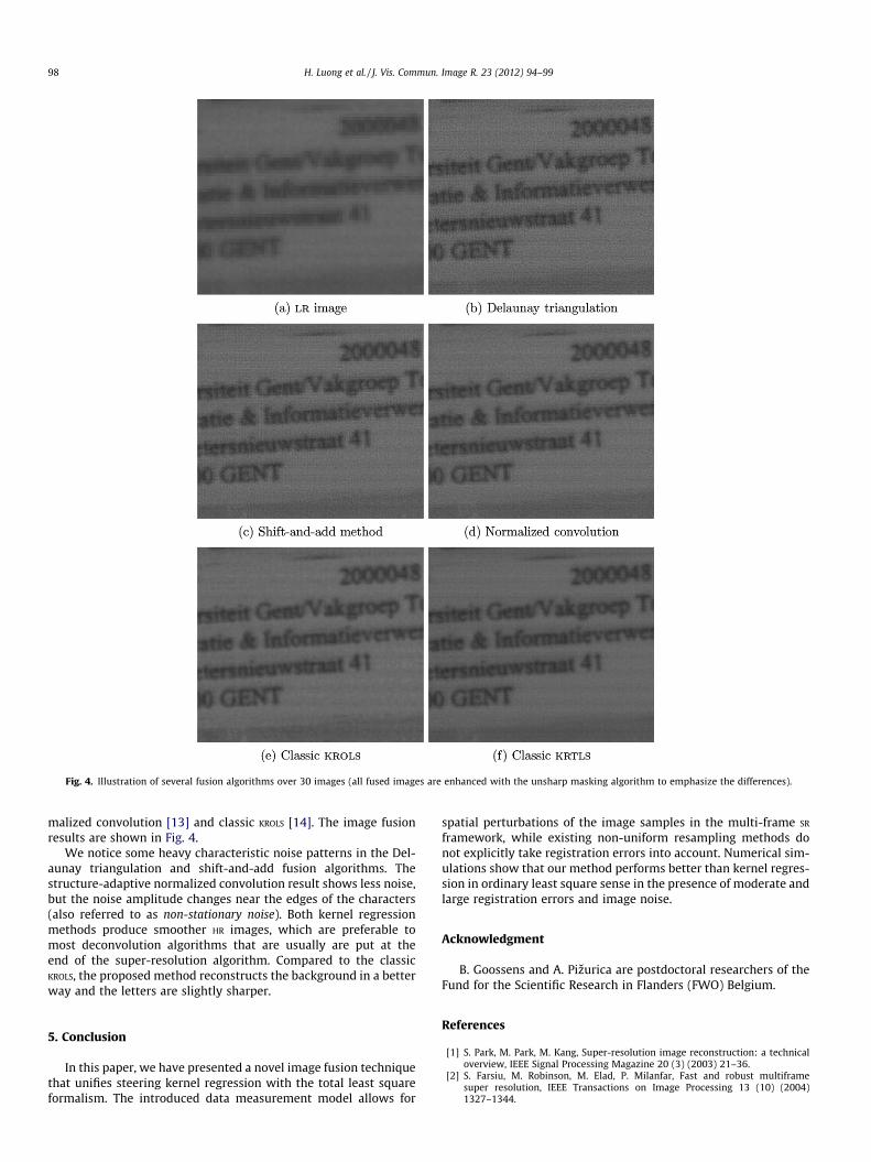
Fig. 4. Illustration of several fusion algorithms over 30 images (all fused images are enhanced with the unsharp masking algorithm to emphasize the differences).

98 H. Luong et al. / J. Vis. Commun. Image R. 23 (2012) 94–99

malized convolution [13] and classic KROLS [14]. The image fusionresults are shown in Fig. 4.

We notice some heavy characteristic noise patterns in the Del-aunay triangulation and shift-and-add fusion algorithms. Thestructure-adaptive normalized convolution result shows less noise,but the noise amplitude changes near the edges of the characters(also referred to as non-stationary noise). Both kernel regressionmethods produce smoother HR images, which are preferable tomost deconvolution algorithms that are usually are put at theend of the super-resolution algorithm. Compared to the classicKROLS, the proposed method reconstructs the background in a betterway and the letters are slightly sharper.

5. Conclusion

In this paper, we have presented a novel image fusion techniquethat unifies steering kernel regression with the total least squareformalism. The introduced data measurement model allows for

spatial perturbations of the image samples in the multi-frame SR

framework, while existing non-uniform resampling methods donot explicitly take registration errors into account. Numerical sim-ulations show that our method performs better than kernel regres-sion in ordinary least square sense in the presence of moderate andlarge registration errors and image noise.

Acknowledgment

B. Goossens and A. Pizurica are postdoctoral researchers of theFund for the Scientific Research in Flanders (FWO) Belgium.

References

[1] S. Park, M. Park, M. Kang, Super-resolution image reconstruction: a technicaloverview, IEEE Signal Processing Magazine 20 (3) (2003) 21–36.

[2] S. Farsiu, M. Robinson, M. Elad, P. Milanfar, Fast and robust multiframesuper resolution, IEEE Transactions on Image Processing 13 (10) (2004)1327–1344.

H. Luong et al. / J. Vis. Commun. Image R. 23 (2012) 94–99 99

[3] M. Unser, Sampling – 50 years after Shannon, Proceedings of the IEEE 88 (4)(2000) 569–587.

[4] C. Glasbey, K. Mardia, A review of image warping methods, Journal of AppliedStatistics 25 (1998) 155–171.

[5] S. Lertrattanapanich, N. Bose, HR image from multiframe by Delaunaytriangulation: a synopsis, in: Proceedings of IEEE International Conference onImage Processing (ICIP), vol. 2, 2002, pp. 869–872.

[6] N. Nguyen, P. Milanfar, A wavelet-based interpolation-restoration method forsuperresolution (wavelet superresolution), Circuits Systems Signal Process 19(4) (2000) 321–338.

[7] R. Gerchberg, Super-resolution through error energy reduction, Optica Acta 21(9) (1974) 709–720.

[8] A. Papoulis, A new algorithm in spectral analysis and band-limitedextrapolation, IEEE Transactions on Circuits and Systems 22 (9) (1975) 735–742.

[9] S. Peleg, D. Keren, L. Schweitzer, Improving image resolution using sub-pixelmotion, Pattern Recognition Letters 5 (3) (1987) 223–226.

[10] A. Fruchter, R. Hook, Drizzle: a method for the linear reconstruction ofundersampled images, Publications of the Astronomical Society of the Pacific114 (792) (2002) 144–152.

[11] Z. Jiang, T.-T. Wong, H. Bao, Practical super-resolution from dynamic videosequences, in: Proceedings of IEEE Computer Society Conference on ComputerVision and Pattern Recognition (CVPR), vol. 2, 2003, p. 549.

[12] E. Nadaraya, On estimating regression, Theory of Probability and itsApplications 9 (1) (1964) 141–142.

[13] T. Pham, L. Van Vliet, K. Schutte, Robust fusion of irregularly sampled datausing adaptive normalized convolution, EURASIP Journal on Applied SignalProcessing 2006 (2006) 1–12.

[14] H. Takeda, S. Farsiu, P. Milanfar, Kernel regression for image processing andreconstruction, IEEE Transactions on Image Processing 16 (2) (2007)349–366.

[15] C. van Wijk, R. Truyen, R. van Gelder, L. van Vliet, F. Vos, On normalizedconvolution to measure curvature features for automatic polyp detection, in:Proceedings of Medical Image Computing and Computer Assisted Intervention(MICCAI), Lecture Notes in Computer Science, Springer-Verlag, vol. 3216, 2004,pp. 200–208.

[16] H. Knutsson, C. Westin, Normalized and differential convolution: Methods forinterpolation and filtering of incomplete and uncertain data, in: Proceedings ofIEEE Conference on Computer Vision and Pattern Recognition (CVPR), 1993,pp. 515–523.

[17] I. Markovsky, S. Van Huffel, Overview of total least-squares methods, SignalProcessing 87 (2007) 2283–2302.

[18] S. Ahn, W. Rauh, H. Cho, H.-J. Warnecke, Orthogonal distance fitting of implicitcurve and surfaces, IEEE Transactions on Pattern Analysis and MachineIntelligence 24 (5) (2002) 620–638.