toronto lectures on physics - fields institute · toronto lectures on physics shlomo sternberg...
TRANSCRIPT

Toronto Lectures on Physics
Shlomo Sternberg
January 3, 2008
Contents
1 The “Standard Model” and some of its ills. 4
2 Problems of translation between mathematics and physics. 52.1 Is there an i in the structure constants of a Lie algebra? . . . . . 52.2 Ad invariant metrics on u(2). . . . . . . . . . . . . . . . . . . . . 62.3 Ad invariant metrics, coupling constants, and the Weinberg angle. 62.4 What are classical fields? . . . . . . . . . . . . . . . . . . . . . . 7
3 The permittivity of space-time is a metric on u(1). 83.1 Electrostatics. . . . . . . . . . . . . . . . . . . . . . . . . . . . . . 8
3.1.1 The electric field. . . . . . . . . . . . . . . . . . . . . . . . 83.1.2 The dielectric displacement. . . . . . . . . . . . . . . . . . 83.1.3 The dielectric operator and the dielectric coefficient. . . . 93.1.4 The dielectric coefficient. . . . . . . . . . . . . . . . . . . 103.1.5 Rotationally invariant solutions of Laplace’s equation. . . 10
3.2 Magnetoquasistatics. . . . . . . . . . . . . . . . . . . . . . . . . . 113.2.1 Objects: The magnetic induction and the magnetic exci-
tation. . . . . . . . . . . . . . . . . . . . . . . . . . . . . . 113.2.2 The laws. 1: Faraday’s law of induction. . . . . . . . . . . 123.2.3 The laws. 2: There are no magnetic poles. . . . . . . . . . 123.2.4 The laws. 3: Ampere’s law. . . . . . . . . . . . . . . . . . 123.2.5 The force on a moving charge. . . . . . . . . . . . . . . . 123.2.6 The permeability. . . . . . . . . . . . . . . . . . . . . . . . 133.2.7 The units of
∫SB. . . . . . . . . . . . . . . . . . . . . . . 13
3.3 The Maxwell equations. . . . . . . . . . . . . . . . . . . . . . . . 133.3.1 The equation dF = 0. . . . . . . . . . . . . . . . . . . . . 133.3.2 The equation dG = 4πj. . . . . . . . . . . . . . . . . . . . 14
3.4 Units. . . . . . . . . . . . . . . . . . . . . . . . . . . . . . . . . . 143.4.1 The units of the integral of F over a surface. . . . . . . . 143.4.2 The units of the integral of G over a surface. . . . . . . . 153.4.3 The integral of F ∧G over a four dimensional region is a
scalar. . . . . . . . . . . . . . . . . . . . . . . . . . . . . . 153.4.4 The units of the permittivity. . . . . . . . . . . . . . . . . 15
1

3.4.5 The units of the permeability. . . . . . . . . . . . . . . . . 163.4.6 ε0 × µ0 = 1/c2. . . . . . . . . . . . . . . . . . . . . . . . . 163.4.7 The permittivity and the permeability in natural units. . 163.4.8 The fine structure constant. . . . . . . . . . . . . . . . . . 16
4 Gauge theories. 17
5 The Higgs mechanism. 185.1 The Higgs mechanism in a nutshell. . . . . . . . . . . . . . . . . 18
5.1.1 The Weinberg angle, again. . . . . . . . . . . . . . . . . . 205.1.2 Scalar products from representations. . . . . . . . . . . . 215.1.3 The Weinberg angle of the fundamental representation of
sl(2/1). . . . . . . . . . . . . . . . . . . . . . . . . . . . . 215.2 Other quadratic forms. . . . . . . . . . . . . . . . . . . . . . . . . 21
5.2.1 Experimental determination of the coupling constant g2. . 235.3 The Higgs mass. . . . . . . . . . . . . . . . . . . . . . . . . . . . 24
6 Using superconnections. 256.1 The metric on the Higgs. . . . . . . . . . . . . . . . . . . . . . . 26
7 Superconnections. 267.1 Superspaces and superalgebras. . . . . . . . . . . . . . . . . . . . 267.2 The tensor product of two superalgebras. . . . . . . . . . . . . . 277.3 Lie superalgebras. . . . . . . . . . . . . . . . . . . . . . . . . . . 287.4 The endomorphism algebra of a superspace. . . . . . . . . . . . . 287.5 Superbundles. . . . . . . . . . . . . . . . . . . . . . . . . . . . . . 287.6 The endomorphism bundle of a superbundle. . . . . . . . . . . . 297.7 The centralizer of multiplication by differential forms. . . . . . . 297.8 Bundles of Lie superalgebras. . . . . . . . . . . . . . . . . . . . . 297.9 Superconnections. . . . . . . . . . . . . . . . . . . . . . . . . . . 307.10 Extending superconnections to the bundle of endomorphisms. . . 307.11 Supercurvature. . . . . . . . . . . . . . . . . . . . . . . . . . . . . 317.12 The tensor product of two superconnections. . . . . . . . . . . . 317.13 The exterior components of a superconnection. . . . . . . . . . . 327.14 A local computation. . . . . . . . . . . . . . . . . . . . . . . . . . 327.15 Superconnections and principal bundles. . . . . . . . . . . . . . . 337.16 The Higgs field and superconnections. . . . . . . . . . . . . . . . 367.17 Clifford Bundles and Clifford superconnections. . . . . . . . . . . 367.18 The Dirac operator of a Clifford superconnection. . . . . . . . . . 37
7.18.1 The exterior algebra as a Clifford module. . . . . . . . . . 377.18.2 The Dirac operator. . . . . . . . . . . . . . . . . . . . . . 387.18.3 A local description of the Dirac operator. . . . . . . . . . 38
7.19 Clifford bundles and spinors. . . . . . . . . . . . . . . . . . . . . 397.20 Facts about Dirac spinors. . . . . . . . . . . . . . . . . . . . . . . 40
7.20.1 The element γ in general. . . . . . . . . . . . . . . . . . . 407.20.2 Majorana spinors for C(q + 2, 2). . . . . . . . . . . . . . . 41
2

7.20.3 Majorana spinors in four dimensions. . . . . . . . . . . . . 417.20.4 A model for the Majorana spinors. . . . . . . . . . . . . . 427.20.5 Bilinear covariants for Majorana spinors. . . . . . . . . . 447.20.6 The Dirac equation for Majorana spinors. . . . . . . . . . 477.20.7 Complexifying a vector space with a complex structure. . 487.20.8 Sesquilinear covariants for Dirac spinors. . . . . . . . . . . 51
8 Special representations of sl(m/n). 538.1 The definition of the Lie superalgebras sl(m/n). . . . . . . . . . 538.2 The representation of sl(V0/V1) on the super exterior algebra of V . 548.3 Special representations of sl(m/1). . . . . . . . . . . . . . . . . . 57
9 sl(2/1) and the electroweak isospins and hypercharges. 589.1 b = 0 - the leptons. . . . . . . . . . . . . . . . . . . . . . . . . . . 599.2 b = 2
3 - the quarks. . . . . . . . . . . . . . . . . . . . . . . . . . . 599.3 b = 1 - the anti-leptons. . . . . . . . . . . . . . . . . . . . . . . . 609.4 b = 1
3 - the anti-quarks. . . . . . . . . . . . . . . . . . . . . . . . 60
10 Using sl(m/1) for m = 3, 5, and 5 + n. 6010.1 m = 3 - unifying quarks and leptons. . . . . . . . . . . . . . . . . 6010.2 m = 5 - including color. . . . . . . . . . . . . . . . . . . . . . . . 6110.3 m = 5 + n - accomodating 2n generations. . . . . . . . . . . . . . 61
11 sl(7/1) - unifying color and four generations. 62
12 sl(6/1). 65
13 Hermitian Lie algebras. 6713.1 The Lie superalgebra su(2/1) and the Lie algebra su(3). . . . . . 6713.2 The general definition. . . . . . . . . . . . . . . . . . . . . . . . . 6913.3 The unitary algebras. . . . . . . . . . . . . . . . . . . . . . . . . 6913.4 su(2, 2/1) and the superconformal superalgebra of Wess and Zu-
mino. . . . . . . . . . . . . . . . . . . . . . . . . . . . . . . . . . 70
14 Renormalization of the supergroup couplings and the Higgsmass. 72I have been invited by the mathematicians here at Toronto to give three
talks describing my joint work with the late Prof. Yuval Ne’eman in elementaryparticle physics. This work uses some mathematical ideas such as super Liealgebras and their representations, and the Quillen theory of superconnections.But the work is in physics, and this puts me in a quandary as to the amount ofphysics background that I can assume.
In order not to chase away any physicists in the audience, I will start bylisting the physics problems that our approach tries to partially address. Thiswill involve some words that may not be familiar to mathematicians, to whom Iapologize. I hope to elucidate the meaning of most of these words in the courseof the lectures. All of the results in these lectures are contained in the review
3

article I wrote with Prof. Ne’eman, and which appeared in Physics Reports 4062005, 303 -377.
I include here some expository material (mainly for mathematicians) whichI did not have time to include in the lectures; for example a review of classicalelectromagnetism and material on the Dirac operator.
I thank Yael Karshon for helpful comments on this text and the associatedslides.
1 The “Standard Model” and some of its ills.
The “Standard Model” of the physics of particles and fields (assumed to includeall known fundamental interactions except for gravity) is enormously success-ful, with its predictions validated by all experimental tests. In particular, theelectroweak interactions seem to be correctly described by the su(2)×u(1) spon-taneously broken local gauge symmetry. Although the full implementation ofthis (Weinberg-Salam) theory requires quantum field theory, much of its basicstructure can be phrased in terms of classical field theory, see for example, KaneModern Elementary Particle Physics , or, for the more mathematically inclinedreader, Derdzinski Geometry of the Standard Model of Elementary Particles.Note that a comprehensive review intended for particle (or high energy) physi-cists appeared in E.S. Abers and B.W. Lee, “Gauge Theories”, Physics Reports,9C no. 1 1973. So this theory has been successfully around for a long time.
The very success of this theory prompted a number of questions relating toits structure, hypotheses and input. The unresolved issues include
• The large number of free parameters which must be experimentally deter-mined to serve as input into the theory such as the various gauge couplingconstants (including the Weinberg angle), the parameters of Higgs poten-tial, the coupling constants of the matter fields, the eigenvalues of theweak isospin and weak hypercharge for the chiral leptons and fermionsetc.
• As a result, the theory is unable to predict the value of the mass of theHiggs particle. This meson has therefore been searched for all over theaccelerator-available spectrum, from a few GeV to the 115 GeV reachedat Cern in October 2000, when 9 “events” were reported at the limitof the accelerator’s energy range. (These “events” constituted 2.6 stan-dard deviations above background level, whereas 5 standard deviations areconsidered necessary for an accepted result that could be interpreted asevidence for the Higgs particle.) All this was before the planned closure ofthe machine. However when the accelerator was granted another month ofoperation, no further evidence was found. Several machines are expectedto renew the search in the next 1- 3 years, reaching into the 100-500 GeVrange.
• The lack of correlation between the quantum numbers of left and rightchiral leptons and fermions.
4

• The ad hoc introduction of Higgs fields to implement spontaneous sym-metry breaking.
• The fact that these Higgs fields constitute a weak isospin doublet.
• No explanation of the origin of the Higgs potential needed to achieveGoldstone-Higgs spontaneous symmetry breaking.
• No explanation of the absence of right handed neutrinos. In fact, since wenow know that the neutrino is massive, we know that right handed neu-trinos do exist. So we can reformulate the question as follows: Why don’tthe right handed neutrinos participate in the Weinberg-Salam theory?
I wish to show in these lectures how using superconnections allows an answerto some of these difficulties.
2 Problems of translation between mathematicsand physics.
There are several communications difficulties between mathematicians and physi-cists, some more serious than others. I want to get a few of these out into theopen before one group or the other disappears:
2.1 Is there an i in the structure constants of a Lie alge-bra?
The first barrier between the mathematics literature and most of the physicsliterature is the ubiquitous factor of i: The mathematical definition of a Liealgebra is that it is a vector space k with a bilinear map
k× k→ k
which is anti-symmetric and satisfies Jacobi’s identity.So the set of self-adjoint matrices under commutator bracket is not a Lie
algebra. Indeed the commutator of two self adjoint matrices is skew adjoint. Sothe Lie algebra of u(n) is not the space of self-adjoint matrices but rather thespace of skew adjoint matrices. Indeed, if A is a skew adjoint matrix then exp tAis a one parameter group of unitary matrices. The physicists prefer to writeexp itH where H is self adjoint. This is of course due to the fact that self adjointoperators are the observables of quantum mechanics, and Noether’s theoremsuggests that elements of the Lie algebra should correspond to observables. Butthe price to pay for this is to put an i in front of all brackets.
For example, the three dimensional real vector space consisting of self adjointtwo by two matrices of trace zero has, as a basis, τi, i = 1, 2, 3 the “Paulimatrices”, where, to be absolutely sure of the factors 1/2 etc.,
τ1 :=(
0 11 0
), τ2 :=
(0 −ii 0
), τ3 :=
(1 00 −1
).
5

The physicists like to think of these as “generators” of SU(2), i.e. as ele-ments of the Lie algebra su(2). Of course, we mathematicians would say thatmultiplying each of these three matrices by i gives a basis of su(2). This dis-tinction is relatively harmless, but is a nuisance for a mathematician reading aphysics book or paper.
2.2 Ad invariant metrics on u(2).
If we use the scalar product
(A,B) = 2 trAB
then the elements 12τi form an orthonormal basis of our three dimensional space
of self-adjoint matrices of trace zero. Since the algebra su(2) is simple, themost general Ad invariant scalar product on our three dimensional space of self-adjoint matrices of trace zero must be a positive multiple of the above scalarproduct.
We will want to consider the four dimensional space of all two by two selfadjoint matrices. (After multiplication by i this would yield the Lie algebra ofU(2).) So we must add the two by two identity matrix I to get a basis of thisfour dimensional real space. The algebra u(2) ∼ su(2)⊕ u(1) is not simple, butdecomposes into the sum of two ideals consisting of su(2) and all (real) multiplesof iI. These ideals must be orthogonal under any Ad invariant metric. So thereis a two parameter family of Ad invariant metrics on u(2).
2.3 Ad invariant metrics, coupling constants, and the Wein-berg angle.
Indeed, the most general Ad invariant metric on our four dimensional space ofall self-adjoint two by two matrices can be written as
2g22
tr(A− 12
(trA)I)(B − 12
(trB)I) +1g21
trA trB. (1)
Relative to this scalar product the elements
g22τ1,
g22τ2,
g22τ3,
g12I (2)
form an orthonormal basis.Notice that for traceless matrices the second term in (1) vanishes, and the
first term reduces to a multiple of 2 trAB; similarly, for multiples of I, the firstterm vanishes.
For mathematicians, the question is “why this strange notation, with theg2 and g1 occurring in the denominator?”. The answer is that, in the physicsliterature, these constants are not regarded as parametrizing metrics on u(2),but rather as “universal coupling constants”. I will spend a chunk of today’s
6

lecture explaining why choosing a metric on a Lie algebra is important, andwhat is its physical significance.
In any event, however you want to interpret these parameters, the Weinbergangle θW is defined by
g21
g22
= tan2 θW .
It plays an important role in the theory.
2.4 What are classical fields?
A third difference between the mathematical literature and the physics litera-ture is that in the physics literature all (classical) fields are regarded as scalarvalued functions (or vector fields) or n-tuplets of scalar valued functions (orvector fields) . One must then discuss the “field transformations” under which,for example, the Lagrangian is invariant. The mathematical literature prefersa “basis free” formulation where many of the invariance properties of the La-grangian are obvious - they are built into the formulation. The price to payis that the fields are no longer scalar functions or n-tuplets of scalar functionsbut vector valued functions, or, more generally, sections of a vector bundle, ordifferential forms with values in a vector bundle.
This means that in the physics literature a basis of the vector space (or abasis of sections of the vector bundle) is chosen. Thus, for example, if we choosea basis v1, . . . , vn of a Lie algebra k then the Lie bracket can be given in termsof the Cartan structure constants c`jk where
[vj , vk] =∑`
c`jkv`.
As explained above, in the physics literature there will be an additional factorof i in front of the structure constants as understood by the mathematicians.For example, if we take the orthonormal basis of the space of traceless two bytwo self adjoint matrices consisting of the first three elements of (2), we find bydirect computation that[g
2τ1,
g
2τ2
]= i
g2
2τ3 = ig
g
2τ3, g = g2,
with a similar formula for the brackets of the remaining two elements. So relativeto this basis, the structure constants are
Cjk` = igεjk`.
Up to an overall sign arising from slightly different conventions this is the state-ment about the structure constants of SU(2)L found in S. Weinberg, The Quan-tum Theory of Fields, Cambridge U. Press (1996), vol. 2. page 307 just afterequation (21.3.11) giving the expression of the Lagrangian of the Yang-Millsfield. So whereas for mathematicians the parameter g describes the scalar prod-uct on su(2), for physicists, who write out the fields in terms of an orthonormal
7

basis, the g appears in the structure constants and is interpreted as a “couplingconstant”, measuring the “strength of the interaction between the fields”.
3 The permittivity of space-time is a metric onu(1).
In order to bolster my contention that the metric on a Lie algebra has importantphysical significance, I want to review Maxwell’s classical theory of electromag-netism, with special attention to units.
I will begin with two non-relativistic regimes:
3.1 Electrostatics.
The objects are:
3.1.1 The electric field.
This is a linear differential form, E, called the electric field strength. A pointcharge e experiences the force eE. The integral of E along any path gives thevoltage drop along that path. The units of E are
voltagelength
=energy
charge · length.
Remember that force has the units energy/length and voltage has units en-ergy/charge.
The fundamental law satisfied by E is
dE = 0.
In simply connected regions this implies the existence of a function u called thepotential such that
E = −du.
3.1.2 The dielectric displacement.
This is a two form D on R3. Its physical significance is as follows. To determinethe value of D on a (small) oriented plane element, insert two small metal platesof the shape of this plane element, touch them together and then separate them.Charges ±Q are acquired on the plates. The orientation of the plane togetherwith the orientation of R3 determines which of these two separated plates is the“top” plate and the value of D is (the limit of)
4πcharge on the top plate
area of the plates.
So the units of D arechargearea
.
8

Notice that this definition makes no mention of the electric field.The fundamental law satisfied by D is Gauss’s law which asserts that for
any region U ∫∂U
D = 4π∫U
ρdx ∧ dy ∧ dz
where ρ is the electric charge density.Stokes’ theorem gives the infinitesimal version of Gauss’s law as
dD = 4πρdx ∧ dy ∧ dz.
If E is an electric field strength and D is a dielectric displacement then E∧Dis a three form which we may integrate over R3 if it is of compact support or ifit vanishes sufficiently rapidly at infinity. Then we can form
〈D,E〉 :=∫R3
E ∧D
which we can consider as a sort of pairing between the space of electric fieldsand the space of dielectric displacements. The value of this pairing has units
volume · forcecharge
· chargearea
= force · length = energy.
3.1.3 The dielectric operator and the dielectric coefficient.
This is a map C from the space of electric fields to the space of dielectricdisplacements. Later on we shall be more specific as to the form of C in termsof the three dimensional ? operator. At the moment we can do with the followingmild assumptions:
• C is linear.
• C is local in the sense that it E vanishes on an open set U so does C(E).
• C is symmetric in the sense that
〈C(E), E〉 = 〈C(E), E〉
when both sides are defined. When both sides are defined, we set
(E, E) := 〈C(E), E〉.
We can then define the energy of an electric field as
12
(E,E).
9

3.1.4 The dielectric coefficient.
A more specific choice of the dielectric operator is to take
C(E) = ε ? E
where ? is the three dimensional star operator mapping one forms into twoforms and ε is a function. Even more specifically, in many cases (such as for thevacuum) ε is a constant - called the dielectric constant. We will postponethe issue of units for the moment, assume that ε is indeed constant, and thenchoose our units of length so that it is absorbed into the star operator. Thenthe equations of electrostatics becomes
E = −duD = ?E
dD = 4πρdx ∧ dy ∧ dzso
∂2u
∂x2+∂2u
∂y2+∂2u
∂z2= −4πρ.
If ρ = 0 in some region, then in that region the last equation becomes Laplace’sequation which we can write in coordinate free notation as
d ? du = 0.
3.1.5 Rotationally invariant solutions of Laplace’s equation.
In polar coordinates we have
?dr = r2 sin θdθ ∧ dφ.
So if f = f(r) is defined for r > 0 we have
df = f ′(r)dr?df = (r2f ′(r)) sin θdθ ∧ dφ
d ? df =(r2f ′(r)
)′dr ∧ sin θdθ ∧ dφ
sod ? df = 0 ⇒
(r2f ′(r)
)′= 0
⇒ r2f ′(r) = −c (a constant)⇒
f(r) =c
r+A
where c and A are constants.The inverse square law of high-school physics drops out.
10

Exactly the same computation yields the Yukawa potential as the staticfundamental solution of the Klein-Gordon equation: Indeed
d
(e−mr
r
)= −e−mrmr + 1
r2dr
so
?d
(e−mr
r
)= −e−mr(mr + 1) sin θdθ ∧ dφ
and hence
d ? d
(e−mr
r
)= m2re−mr sin θdr ∧ dθ ∧ dφ
= m2
(e−mr
r
)r2 sin θdr ∧ dθ ∧ dφ.
Thus if we think of a solution of the Klein-Gordon equation or of the Procaequation as a “transmitter” of a “force”, then the value of m determines therange of this force.
3.2 Magnetoquasistatics.
3.2.1 Objects: The magnetic induction and the magnetic excitation.
The magnetic induction is a two form B on R3, which exerts a force on a currentaccording to the following rule: if a charge emoves past the point P with velocityv then the force exerted on that charge is the covector
ei(v)BP .
At each point of space the form B if 6= 0 will determine a direction in space:the line determined by the equation
i(w)B = 0.
Iron filings free to rotate but not to move will align themselves in these direc-tions, producing the “magnetic lines of force” favored by Faraday. These areprecisely the directions in which a current will feel no force.
The second item is a one form H known as the magnetic excitation. Thesecond of Ampere’s laws says that if S is any surface bounded by a curve γ, andif J is the two form representing the current flow, then∫
γ
H = 4π∫S
J.
11

3.2.2 The laws. 1: Faraday’s law of induction.
This says that if S is a surface bounded by a curve γ then
− d
dt
∫S
B =∫γ
E. (3)
By Stokes the differential version of this law is
∂B
∂t= −dE. (4)
If S is a closed surface bounding a region (so with no boundary curves) thenFaraday’s law implies that
d
dt
∫S
B = 0.
In fact, a stronger law holds (Hertz), not only does the derivative of the integralof B over a closed surface vanish, but the integral itself does:
3.2.3 The laws. 2: There are no magnetic poles.
This says that ∫S
B = 0 for any closed surface S.
By Stokes, the differential version of this law is
dB = 0.
3.2.4 The laws. 3: Ampere’s law.
Recall that this says that if S is any surface bounded by a curve γ, and if J isthe two form representing the current flow, then∫
γ
H = 4π∫S
J.
By Stokes’ theorem, the differential version of this law is
dH = 4πJ.
3.2.5 The force on a moving charge.
The force exerted by a magnetic field B on a moving charge I = ev is
i(I)B.
12
3.2.6 The permeability.
There is a relation between H and B given by
B = µ ? H
where ? is the three dimensional star operator and µ is known as the perme-ability.
3.2.7 The units of∫SB.
By Faradays’ law of induction, the time derivative of this integral over a surfacebounded by a curve is equal to the negative of the integral of E around thatcurve which has units of voltage which is energy/charge. So
units of∫ ∫
SB
time=
energycharge
.
In “natural units”, where ~ = 1, energy has units of inverse time. This impliesthat the integral of B over a surface has units of inverse charge.
3.3 The Maxwell equations.
The laws of quasi-magnetostatics take on a very suggestive form when writtenin four dimensions rather than three, and when an important modification toAmpere’s law is made. This modification was introduced by Maxwell.
3.3.1 The equation dF = 0.
We can combine the laws
dB = 0 (Hertz)
∂B
∂t= −dE (Faraday’s law of induction)
into the single lawdF = 0 (5)
if we setF = B + E ∧ dt.
In (5) the operator d means the four dimensional (space-time) d. The coefficientof dx ∧ dy ∧ dz in (5) says that
dspaceB = 0 (Hertz)
while the coefficient of dt in (5) gives Faraday’s law of induction.The equation dF = 0 implies that locally we can find a one form A (called
the four potential) such thatdA = F. (6)
13
3.3.2 The equation dG = 4πj.
In electrostatics we assumed that J = 0 and that the charge density ρ did notdepend on t. In quasi-magnetostatics we ignored ρ. For the full equations ofelectromagnetism one assumes that there is a charge density and a current, andso consider the three form
j := ρdx ∧ dy ∧ dz − J ∧ dt
on space time. “Conservation of charge” then demands that
dj = 0.
Locally this says that there is two form G such that
dG = 4πj. (7)
(The 4π is conventional.) If we write
G = D −H ∧ dt, (8)
then the dt component of (7) is
dspaceH =∂D
∂t+ 4πJ.
So we recover Ampere’s law with the modification that the “displacement cur-rent”
∂D
∂t
is added to the right hand side of Ampere’s original law. The “space component”of (7) is
dspaceD = 4πρdx ∧ dy ∧ dzas in electrostatics.
3.4 Units.
Let us work in natural units where ~ = 1 so that energy has units of inversetime.
3.4.1 The units of the integral of F over a surface.
We have already observed that the integral of B over a surface has units ofinverse charge. The integral of E over a curve has units of (energy)/(charge),so the integral of E ∧ dt over a surface in space time has units of
(energy)× (time)(charge)
=1
(charge).
In short, the integral of F over a surface in space time has units of inversecharge.
14

3.4.2 The units of the integral of G over a surface.
From its definition, or from Gauss’s law dD = 4πρdx ∧ dy ∧ dz we see that theunits of the integral of D over a surface are charge. Ampere’s law
dspaceH =∂D
∂t+ 4πJ
together with Stokes’ theorem says that the integral of H over a curve hasthe same units as the flux of current through a surface and this has units(charge)/(time). So the integral of H ∧ dt over a surface in space time alsohas the units of (charge). In short, the integral of G over a surface in space timehas units of charge.
3.4.3 The integral of F ∧G over a four dimensional region is a scalar.
This follows from the preceding two results. In particular, this means that Gis in a sense “dual” to F , the duality being given by exterior multiplicationfollowed by integration. Of course we can not expect that the integral overall of space time will converge. We will examine this“duality” in more detailfurther on.
Notice that until now we have not used the metric structure of space time.
3.4.4 The units of the permittivity.
The unitsD are (charge)/(area). The units of E are (energy)/(charge)×(length).If there is a point-wise matrix which expresses the coefficients of D in terms ofthose of E its entries will have units
chargearea
× (charge)× (length)energy
=(charge)2
(energy)× (length).
Indeed, the permittivity of free space is a scalar ε0 given by
ε0 = 8.854187...× 10−12 Faradmeter
where the Farad is a unit of capacitance:
1 Farad := 1coulomb
volt.
Since1 volt = 1
joulecoulomb
has units of (energy)/(charge) we see that ε0 has units of
(charge)2
(energy)× (length).
15

3.4.5 The units of the permeability.
According to Ampere’s law the units of H are (charge)/(length)×(time).According to Faraday’s law the units ofB are (energy)×(time) / (charge)×(length2.
If there is a point-wise matrix which expresses the coefficients of B in terms ofthose of H its entries will have units
energy× (time)2
(charge)2 × (length).
Indeed, the permeability of free space is a scalar µ0 given by
µ0 = 12.566370 × 10⁻⁷ joule(amp)2 × (meter)
.
Since one amp = one (coulomb)/(second) we see that µ0 does have the abovestated units.
3.4.6 ε0 × µ0 = 1/c2.
This was of course another of the great discoveries of Maxwell and verified byHertz. We can see that the product of the units of the permittivity with thoseof the permeabilty yield units of 1/(velocity)2, and doing the multiplication forthe values of free space give the velocity of light, implying that light consists ofelectromagnetic propagation.
As a consequence, we can choose units in which c = 1 and lengths and timesare measured in the same units. Special relativity with its Minkowski metricdt2 − dx2 − dy2 − dz2 is then an immediate consequence.
3.4.7 The permittivity and the permeability in natural units.
If we choose natural units so that ~ = 1 and c = 1 then length has the sameunits as time and so energy has units of inverse length and the expressionin the denominator for the units of the permeability is just a scalar. So thepermittiviity has units of (charge)2.
Similarly, the units of the permeability become (charge)−2.
3.4.8 The fine structure constant.
The expression
α :=(charge of the electron)2
4πε0is a pure number in terms of our natural units where ~ = 1 and c = 1 and isequal to
1137.0359...
.
In terms of conventional units we would write
α =e2
4πε0~c.
16
4 Gauge theories.
Hermann Weyl had suggested that the true objects of general relativity shouldnot be (semi-)Riemann metrics, but rather the associated Levi-Civita connec-tion. And if we generalize this connection to be a conformal connection (i.e.if we enlarge the group from O(1, 3) to R+ × O(1, 3)) then we can incorporateelectromagnetism.(See his classic Raum Zeit Materie, Springer, Berlin (1918)).The word “gauge” derives from Weyl’s theory in which the length is changedby a conformal transformation.
Einstein rejected Weyl’s proposal of considering a conformal connection asthe underlying physical field, although Einstein himself considered the possibil-ity that Riemannian geometry be replaced by conformal geometry as a basisfor unified theories - see his article in Preuss Akad. 261 (1921) as well as thefollowing notes on the “unified field theory”: loc. cit. (1925) p. 414, (1928) p.3, (1929) p. 3.
After the advent of quantum mechanics, Fritz London, in a short note in early1927(F. London, “Die Theorie von Weyl und die Quantenmechanik”, Natur-wiss. 15 187. and soon after in a longer paper, “Quantenmechanische Deutungder Theorie von Weyl,” Zeit. fur Physik 42, 375-389 (1927), proposed a quan-tum mechanical interpretation of Weyl’s attempt to unify electromagnetism andgravitation. The essential idea is to replace Weyl’s R+ by U(1) acting as phasetransformations of the quantum mechanical state vector. The group U(1) doesnot act on the tangent space of space time. It is “internal”. The London theoryfor U(1) was generalized to SU(2) by Yang and Mills in 1954, C.N. Yang and R.Mills, “Conservation of isotopic spin and isospin gauge invariance,” Phys. Rev.96 191-195 (1954).
The “field” in a Yang-Mills theory on space time is a connection on a prin-cipal bundle P .
Giving a connection on a principal bundle is the same as giving (consistently)the notion of covariant derivative on any associated bundle. The covariantderivative language is more popular in the standard physics texts. I will givea self contained review of the notions of connection and curvature in the moregeneral setting of superconnections and supercurvature later on.
If G is the structure group of the bundle P and g0 is the Lie algebra of G,the curvature of such a connection is a 2-form on space-time with values in thevector bundle g0(P ) associated to the adjoint representation of G. If F is sucha curvature form, and if ? denotes the Hodge star operator of space time, then?F is another 2-form with values in g0(P ), so
F ∧ ?F
is a 4-form with values in g0(P ) ⊗ g0(P ). In order to get a numerical valued4-form which we can consider as a Lagrangian density, we need an Ad invariantscalar product on g0.
For example, we have seen that the electromagnetic field F is a two formwhose integral over any surface has units of inverse charge. So F ∧?F is a 4-form
17

with units of 1/(charge)2. In order to get the correct Lagrangian density, wemust multiply by ε0, the permittivity of empty space which (in natural units)has units of (charge)2, so that
12ε0F ∧ ?F
is the Lagrangian density for the electromagnetic field in empty space. If wewant to consider F (strictly speaking iF ) as the curvature of a connection on aU(1) bundle, we see that we must consider ε0 as determining a metric on u(1)(different from the “natural” one regarding u(1) as iR), and this metric hasdeep physical significance.
In the Standard Model of the electroweak theory, the group under consid-eration is U(2) or SU(2) × U(1) with Lie algebra g0 = u(2). As we have seen,there is a two parameter family of invariant metrics on u(2) given by (1).
We repeat that we are regarding g1 and g2 as parameters describing possibleAd invariant scalar products on the Lie algebra u(2). As such they have physicalsignificance similar to that of the permittivity of free space in electromagnetictheory and are necessary to be able to formulate a Yang-Mills functional. In ageneral relativistic theory one would expect them to have a space time depen-dence just as the metric of space time does. The interpretation of g1 and g2 as“universal coupling constants” then derives from the interpretation as defininga metric.
5 The Higgs mechanism.
5.1 The Higgs mechanism in a nutshell.
The Higgs mechanism in the Standard Model of electroweak interactions is adevice for breaking the u(2) = su(2)⊕u(1) symmetry of a U(2) gauge theory insuch a way that the three of the four components of a connection form (originallymassless in a pure Yang-Mills theory) become differential forms with values ina vector bundle associated to U(1) and which enter into a Lagrangian whosequadratic terms correspond to particles with positive mass. In mathematicalterms this corresponds to a reduction of a principal U(2) bundle to a U(1)bundle.
The ingredients that go into this mechanism and into the computation ofthe acquired masses are the following:
• An Ad invariant positive definite metric on u(2). This is needed for theoriginal (unbroken) Yang-Mills theory. We have argued that the “universalcoupling constants” that enter into the general formulation of this theoryare in fact parameters which describe the possible Ad invariant metrics onu(2). In general there is a two parameter family of such metrics. They arerelated by a certain angle θW known as the Weinberg angle. Our internalsupersymmetry proposal will determine this angle as 300, or sin2 θW =0.25, which is not too far from the measured value of 0.2312± 0.003.
18

• A two dimensional Hermitian vector bundle associated to the principalU(2) bundle. In the general presentation of the Standard Model this vectorbundle is an extraneous ingredient put in “by hand”. In our theory thisvector bundle is g1, the odd component of a Lie super algebra bundle. Thesections of this bundle are regarded as the exterior degree zero componentsof a superconnection. More details on this later.
• A degree-four polynomial on this vector bundle. In the general presenta-tion this must also be provided by hand. In our theory, the quartic termof this polynomial is the super-Yang-Mills functional.
• The vector bundle g1 is associated to the original U(2) bundle, so U(2)invariance determines the Hermitian metric up to a scalar factor. We pro-posed to fix this scalar by relating it to the choice of scale entering intothe metric on su(2). This is done by using the concept of a HermitianLie algebra, see S. Sternberg, J. Wolf, “Hermitian Lie algebras and meta-plectic representations”, Trans. Amer. Math. Soc. 231 1 (1978) whichrelates certain Lie superalgebras to ordinary Lie algebras. Once the met-ric has been fixed, we can write the most general (invariant) degree fourpolynomial as
a‖ · ‖4 − b‖ · ‖2.
The next three steps are part of the standard Higgs mechanism, cf. for exampleA. Derdzinski, Geometry of the standard model Section 11. We summarize themhere for the reader’s convenience. Additional details will be given below.
• If a and b are both positive, then the quadratic polynomial
az2 − bz
achieves its minimum atz0 =
b
2aand hence any section ψ of our vector bundle lying on the three-spherebundle
‖ψ‖2 = z0
is a global minimum. Any such section is called a vacuum state. Thereduction of the principal U(2) bundle is achieved by fixing one such vac-uum. For example, if the bundle is trivial and is given a trivializationwhich identifies it with the trivial C2 bundle then we may choose ψ of theform
ψ = ψ0 :=(
0v
), v > 0
so
‖ψ0‖ =
√b
2a.
19
• The mass of the W particle is then given as
m(W ) =‖ψ0‖‖iτ1‖u(2)
(9)
where
τ1 =(
0 11 0
).
See the discussion in Section 5.2 below. In terms of the parameter g2entering into the definition of the metric on su(2) (see (1)) this becomes
m(W ) =12g2‖ψ0‖ =
12g2
√b
2a. (10)
• The mass of the Higgs field (see Section 5.3 below) is given by
m(Higgs) = 2√b. (11)
This gives the value of the Higgs mass in terms of parameters enteringinto the Higgs model. Notice that only the coefficient of the quadraticterm (b) enters into this formula, but if we know the coefficient a of thequartic term, then we can get b from ‖ψ0‖ =
√b/2a.
As indicated above, we will derive the value of a from the supercurvatureand the metric on the superalgebra coming from a corresponding Lie alge-bra, see equation (15) below. Thus we are able to predict the Higgs massfrom the observed experimental value of the W mass using (10) and (11)and the value of a. We will find that m(Higgs)=2m(W).
To reiterate - we make no predictions about b. We do make a prediction of acoming from the interpretation of the quartic term in the Higgs field as arisingfrom a super-Yang-Mills Lagrangian (to be explained below). No matter whatb is, the knowledge of a determines the ratio of the mass of the Higgs to themass of the W .
5.1.1 The Weinberg angle, again.
We return to equation (1) which gives the most general ad-invariant scalarproduct on u(2). The Weinberg angle is then defined by
g21
g22
= tan2 θW .
Thus, for example, any choice of g1 and g2 which leads to a value of
g21
g22
= 1/3
will yield a Weinberg angle of 30 degrees.
20

5.1.2 Scalar products from representations.
Any faithful unitary representation r of u(2) will yield a positive definite scalarproduct by letting the scalar product of A and B be
− tr r(A)r(B).
Under our identification of u(2) with self adjoint rather than skew adjoint ma-trices, which involves multiplication by i, we can forget about the minus sign.But we do want to allow for an overall scale factor and so consider the metric
A 7→ 2g2
tr(r(A)2
)(12)
as being associated to the representation r. Of course the Weinberg angle willbe independent of the factor g.
So any theory which singles out a preferred faithful representation of u(2)will give a prediction of the Weinberg angle. Our proposal is to regard u(2) asthe even part of the superalgebra su(2/1) ⊂ sl(2/1). See Section 8.1 for thedefinition of the Lie superalgebras sl(m/n). Each of these Lie superalgebrashas a fundamental (defining) representation as described in Section 8.1. Inparticular, this picks out a preferred faithful representation of u(2) and hencegives a prediction of the Weinberg angle. We do the computation in the nextsection.
5.1.3 The Weinberg angle of the fundamental representation of sl(2/1).
In this representation the two by two matrix A is represented by the three bythree matrix
r(A) =(A 00 trA
).
If we take A ∈ su(2) so trA = 0 in (12) we get tr(r(A)2) = tr(A2) from whichwe see that the g2 entering into formula (1) for the metric on u(2) is given byg22 = g2. If we take A = I in (12) we get
r(I) =
1 0 00 1 00 0 2
so tr(r(I)2) = 6. So
2g2· 6 =
4g21
sog21
g22
=13
yielding a Weinberg angle of 30 degrees.
5.2 Other quadratic forms.
Given a positive definite real scalar product (·, ·) on a real vector space, any otherquadratic form is given by x 7→ (Sx, x) where S is a self-adjoint operator. We
21

can then diagonalize S. If the second quadratic form is positive semi-definite,then these eigenvalues are non-negative, and S has a unique square root S
12
with non-negative eigenvalues. For reasons of differential geometry - essentiallythe reduction of a U(2) bundle to a U(1) bundle via the choice of section of anassociated bundle - these eigenvalues are identified with the masses of certainspin 1 particles in the example I will now work out. I will do the elementarylinear algebra now, so we can see what is needed for mass predictions, anddiscuss the geometry later.
For example, consider the standard action of u(2) on C2 and define the“second” quadratic form on u(2) to be
q(A) := ‖Aψ0‖2C2 = (Aψ0, Aψ0)C2
where ψ0 is a fixed element of C2, and where (·, ·)C2 is some U(2) invariantscalar product on C2 (and so is some positive multiple of the standard scalarproduct). The corresponding bilinear form on u(2) is
〈A,B〉 = Re(Aψ0, Bψ0)C2 .
In fact, let us take
ψ0 :=(
0v
), v > 0
as above. Then
τ1ψ0 =(v0
), τ2ψ0 =
(−iv
0
), τ3ψ0 =
(0−v
), and Iψ0 =
(0v
).
Then relative to any scalar product (·, ·) on u(2) we have
(Sτ1, X) = 〈τ1, X〉 = 0 for X = τ2, τ3, I.
If (·, ·) is any of the invariant metrics (1), then (τ1, X) = 0 for X = τ2, τ3, I. Thisshows that τ1 is an eigenvector of S with eigenvalue ‖ψ0‖2/‖τ1‖2u(2). Similarlyfor τ2. Sections of the line bundles corresponding to these eigenvectors areidentified with the W particles. This accounts for the mass of the W as givenin equation (9) above.
We have (τ3 + I)ψ0 = 0 so τ3 + I is an eigenvector of S with eigenvalue0. Expressed in terms of the orthonormal basis (2) and normalized so to havelength one gives
1(g2
1 + g22)
12
(g2g12I + g1
g22τ3
).
The corresponding mass zero field is then identified with the electromagneticfield.
Taking the orthogonal complement of the three eigenvectors found so far(corresponding to the W ’s and the electromagnetic field) gives the field of theZ particle.
22

All of the material in this section is part of the standard repertoire of theHiggs mechanism and is not particular to the model we propose. For instance,equation (9) is the formula in equation (11.30) A. Derdzinski, Geometry of thestandard model for the mass of the W up to differences in notation and the factthat we are computing in natural units.
But it might be instructive to see how all this is written out in the physics lit-erature, where “fields” are always scalar valued. In terms of the basis τ1, τ2, τ3, Iwe have verified that our quadratic form is given by
q(X1τ1 +X2τ2 +X3τ3 + Y I) = v2(X21 +X2
2 + (Y −X3)2).
Let us express this in terms of the coordinates in the orthonormal basis writtenabove (and taking the standard Hermitian form on C2). We have
Xiτ1 =2Xi
g2· g2τi
2
so the coefficient Wi of Xiτi in terms of the normalized basis element is
Wi =2Xi
g2
and henceXi =
g22Wi, i = 1, 2, 3
and similarly Y = g12 B where B is coefficient relative to the last normalized
element. So
Q(W1,W2,W3, B) =14v2(g22(W 2
1 +W 22 ) + (g2W3 − g1B)2
).
The rotation
RθW=
1√g21 + g2
2
(g2 −g1g1 g2
)in the W3, B plane brings the quadratic form to diagonal form. This is thereason for angle terminology. The W1,W2 and Z are considered as transmittersof the weak interaction, while the massless field is identified with the photon.
5.2.1 Experimental determination of the coupling constant g2.
The coupling constant g2 enters into the definition of the metric on u(2) as wehave seen, and is observed via the “strength” of the electro-weak interaction.We have
g2 =e
sin θW.
So if sin θW = 12 we have g2 = 2e. If
e2
4π.=
1137
then g2.= 0.6.
23

5.3 The Higgs mass.
It is assumed that the Higgs field is a section of a Hermitian vector bundle withpotential V which has the form
V(ψ) = f(〈ψ,ψ〉)
wheref : [0,∞)→ R
is a smooth function with a minimum at z0. A particular section is ψ0 chosenwith 〈ψ0, ψ0〉 = z0. (If, as we shall assume, the Hermitian vector bundle is atwo dimensional bundle associated to a principal U(2) or SU(2)× U(1) bundlethis has the effect of reducing the principal bundle to a U(1) bundle.)
The most general section of our vector bundle is then written as ψ0 + η andwe consider the quadratic term in the expansion of f(ψ0 + η) as a function ofη. It will be given by
12
Hess(f)(ψ0)(η) = 2f ′′(〈ψ0, ψ0〉)(Re〈ψ, η〉)2.
For η tangent to the orbit of the action of U(2) this vanishes. But for η ∈ Rψ0 wehave 〈ψ0, η〉 = ±‖ψ0‖‖η‖ so for such η (known as the Higgs field) the quadraticterm is
2z0f ′′(z0)‖η‖2.We want to consider this as a mass term, which means that we want to writethis quadratic expression as 1
2m2‖η‖2.
Iff(z) = az2 − bz
with a and b positive constants, then the minimum of f is achieved at
z0 =b
2a
andf ′′(z0) = 2a.
So2z0f ′′(z0) = 2b.
So we wish to write 2b‖η‖2 as 12m
2‖η‖2 where m is the mass of the Higgs. Thisgives
m(Higgs) = 2√b
as in equation (11) above.Once again, all of the material in this section is part of the standard reper-
toire of the Higgs mechanism and is not particular to the model we propose.Equation (11) is the formula in equation (11.30) of Derdzinski, Geometry ofthe standard model for the Higgs mass up to the fact that we are computing innatural units.
We will now revert to standard notation and write the Higgs field as ψ.
24

6 Using superconnections.
We assume that the Higgs field ψ is the degree zero piece of a superconnectionfor su(2/1), and use this - together with an idea coming from the theory ofHermitian Lie algebras - to predict a value of a, namely
a =18g22 .
I will present a detailed exposition of the theory of superconnections later.But I want to get to the punch line in a hurry. So I will now show how thesuper-Yang-Mills Lagrangian for su(2/1) makes a prediction of the factor aoccurring in the f in the preceding section. In general, the Lagrangian of asuper-Yang-Mills-Higgs theory will be of the form
(1/2)||F ||2 + ...
where F is the supercurvature and where .... involves the fermions, plus aquadratic term in the Higgs whose origin we leave open. The supercurvature isquadratic in the degree zero part of the superconnection, and hence the aboveLagrangian, being quadratic in F , will be quartic in the degree zero part of thesuperconnection. So if we identify the Higgs field with this degree zero part, weget a quartic polynomial in the Higgs which derives from the underlying theorywith no additional ad hoc assumptions. Here are the details of the computation:
If the Higgs field ψ is the degree zero piece of a superconnection for su(2/1),then the supercurvature F will include a term 1
2 [ψ,ψ] which is a section of u(2)regarded as the even part of su(2/1). If
ψ =
0 0 x0 0 yx y 0
then
12
[ψ,ψ] =
|x|2 xy 0xy |y|2 00 0 |x|2 + |y|2
.
To compute ‖F‖2, we need a metric on u(2). In the computation of theWeinberg angle, we took the metric to be proportional to the metric inducedby the fundamental representation of sl(2/1). So we must use the metric
A 7→ 2g22
tr
((A 00 trA
)2)
so as to get the metric (1) on the u(2) component. Applied to the 12 [ψ,ψ] given
above we get4g22
(|x|2 + |y|2)2.
25

Taking 12 of the above expression (as one half of the square length appears in
the Lagrangian) gives the quartic term as
2g22
(|x|2 + |y|2)2. (13)
6.1 The metric on the Higgs.
We need to express (13) as a‖ψ‖4. To do this we must say what ‖ψ‖2 is. We nowuse the paper S. Sternberg, J. Wolf, “Hermitian Lie algebras and metaplecticrepresentations”, Trans. Amer. Math. Soc. 231 1 (1978) and propose that wethink of su(2/1) as the real part of the object whose imaginary part is su(3).
If I have time, I will explain this later.On su(3) the only invariant metrics are scalar multiples of the Killing form,
and since we want the metric to reduce to the above metric on su(2) we mustchoose ‖ψ‖2 as
ψ 7→ 2g22
trψ2 =4g22
(|x|2 + |y|2). (14)
Comparing the two expressions (13) and (14) gives
a =18g22 . (15)
Substituting this into (10) gives
m(W ) =√b. (16)
Comparing with (11) givesm(Higgs)m(W )
= 2. (17)
This was the prediction in [N86]. For later versions of this prediction see [R98]and references cited there.
7 Superconnections.
In this section we give a self contained introduction to the theory of supercon-nections for the convenience of the reader. In the main, we follow the expositiongiven in [BGV91] with some changes in notation. For an alternative treatmentsee [MaSa2000].
7.1 Superspaces and superalgebras.
A superspace E is just a vector space with a Z2 grading:
E = E+ ⊕ E−.
26

A superalgebra A is an algebra whose underlying vector space is a superspaceand such that
A+ ·A+ ⊂ A+, A− ·A− ⊂ A+, A+ ·A− ⊂ A−, A− ·A+ ⊂ A−.
The commutator of two homogeneous elements of A is defined as
[a, b] := ab− (−1)|a|·|b|ba.
We use the notation |a| = 0 if a ∈ A+ and |a| = 1 if a ∈ A− and we do additionand multiplication mod 2.
A superalgebra is commutative if the commutator of any two elements van-ishes. For example, the exterior algebra ∧(V ) of a vector space is a commutativesuperalgebra where
∧(V )+ := ∧0(V )⊕ ∧2(V )⊕ ∧4(V )⊕ · · · ,
and∧(V )− := ∧1(E)⊕ ∧3(V )⊕ · · · .
7.2 The tensor product of two superalgebras.
If A and B are superspaces we make A⊗B into a superspace by
|a⊗ b| = |a|+ |b|.
If A and B are superalgebras we make A⊗B into a superalgebra by
(a⊗ b) · (a′ ⊗ b′) := (−1)|b|·|a′|aa′ ⊗ bb′.
For example, the Clifford algebra of any vector space with a scalar product isa superalgebra, where C(V )+ consists of those elements which can be writtenas a sum of products of an even number of elements of V and C(V )− consistsof those elements which can be written as a sum of products of an odd numberof elements of V . If V and W are two spaces with scalar products then theClifford algebra of their orthogonal direct sum is the tensor product of theirClifford algebras:
C(V ⊕W ) = C(V )⊗ C(W ).
We will use the convention of the algebraists rather than that of the geometersin the definition of the Clifford algebra, W. Greub, Multilinear algebra Springer,Berlin (1978) . So if V is a vector space with a (not necessarily positive definite)scalar product then C(V ) is the universal algebra relative to the relations
uv + vu = 2(u, v)1.
Chevalley, in is classic book does not have the factor 2 on the right hand side,because he considers fields of arbitrary characteristic, including characteristicrwo
(In N. Berline, E. Getzler, M. Vergne: Heat Kernels and Dirac Operators,Springer, Berlin 1991 the opposite convention (with a minus sign on the righthand side) is used.)
27

7.3 Lie superalgebras.
If A is an associative superalgebra the commutator of two homogeneous elementsof A was defined as
[a, b] := ab− (−1)|a|·|b|ba.
This commutator satisfies the axioms for a Lie superalgebra which are
• [a, b] + (−1)|a|·|b|[b, a] = 0, and
• [a, [b, c]] = [[a, b], c] + (−1)|a|·|b|[b, [a, c]].
It was proved in L. Corwin, Y. Ne’eman, S. Sternberg, “Graded Lie algebrasin mathematics and physics”, Rev. Mod. Phy. 47 573 (1975) that every Liesuperaglebra has a universal (associative) enveloping algebra and that the ana-logue of the Poincare-Birkhoff-Witt theorem holds.
If A is a commutative superalgebra and L is a Lie superalgebra then A⊗ Lis again a Lie superalgebra under the usual definition:
[a⊗X, b⊗ Y ] := (−1)|X|·|b|ab⊗ [X,Y ].
7.4 The endomorphism algebra of a superspace.
Let E = E+⊕E− be a superspace. We make the algebra of all endomorphisms(= linear transformations) of E into a superalgebra by letting End(E)+ consistof those linear transformations which carry E+ into E+ and E− into E− whileEnd(E)− interchanges the two components. Thus a typical element of End(E)+
looks like (A 00 D
), A ∈ End(E+), D ∈ End(E−)
while a typical element of End(E)− looks like(0 BC 0
), B : E− → E+, C : E+ → E−.
An action (or a representation) of an associative algebra A on a superspaceE is a (gradation preserving) homomorphism of A into End(E). We then alsosay that E is an A module.
Similarly, a representation of a Lie superalgebra L on a superspace E is ahomomorphism of L into the commutator Lie superalgebra of End(E). This isthe same as an action of the universal enveloping algebra U(L) on E. We saythat E is an L module.
7.5 Superbundles.
Let E → M be a bundle of superspaces over a manifold M . We call such anobject a superbundle. So E = E+ ⊕ E− where E+ → M and E− → M arevector bundles over M . We will call a section of E+ an even section of E and asection of E− an odd section of E .
28

If E and F are superbundles, then E ⊗ F is a superbundle. In particular,∧(T ∗M) is a superbundle where
∧(T ∗M)+ := ∧0(T ∗M)⊕ ∧2(T ∗M)⊕ ∧4(T ∗M)⊕ · · · ,
∧(T ∗M)− := ∧1(T ∗M)⊕ ∧3(T ∗M)⊕ ∧5(T ∗M)⊕ · · · .
A section of ∧(T ∗M) ⊗ E is called an E-valued differential form and thespace of all E-valued differential forms will be denoted by A(M, E). Locally anyelement of A(M, E) is a sum of terms of the form α⊗ s where α is a differentialform on M and s is a section E .
7.6 The endomorphism bundle of a superbundle.
If E → M is a superbundle, then we can consider the superbundle End(E)where, at each m ∈ M we have End(E)m := End(Em). We have an action ofany section of End(E) on any section of E . By tensor product, any element ofA(M,End(E)) acts on any element of A(M, E). In particular any element ofA(M), i.e. any differential form acts on A(M, E) and (super)commutes with allelements of A(M,End(E)).
7.7 The centralizer of multiplication by differential forms.
Any element of A(M), i.e. any differential form, acts on A(M, E) and (su-per)commutes with all elements of A(M,End(E)).
There is an important converse to this last assertion. A differential operatoron A(M, E) is by definition an operator which in local coordinates looks like∑
γ
aγ∂γ
where aγ is a section of EndA(M, E) and ∂γ = ∂γ11 · · · ∂γnn is a partial differen-
tiation operator in terms of the local coordinates. Leibnitz’s rule implies that ifsuch an operator commutes with all multiplications by functions then it can’treally involve any differentiations. If furthermore it commutes with the actionof all elements of A(M) it must be given by the action of some element ofA(M,End(E)). In short: a differential operator on A(M, E) commutes with theaction of A(M) if and only if it is given by an element of A(M,End(E)).
7.8 Bundles of Lie superalgebras.
If g is a bundle of Lie superalgebras over M then A(M, g) is a Lie superalgebrawith bracket determined fiberwise (as we have seen) by
[α⊗X,β ⊗ Y ] = (−1)|X|·|β|(α ∧ β)⊗ [X,Y ].
If E is a superbundle on which g acts, meaning that we have a fiberwise Liesuperalgebra homomorphism ρ of g into the Lie superalgebra bundle End(E)
29

(under fiberwise bracket), then we have an action of A(M, g) on A(M, E) deter-mined by
ρ(α⊗X)(β ⊗ v) = (−1)|X|·|β|(α ∧ β)⊗ (ρ(X)v).
7.9 Superconnections.
A superconnection on a superbundle E is an odd first order differential oper-ator
A : A±(M, E)→ A∓(M, E)
which satisfies
A(α ∧ θ) = dα ∧ θ + (−1)|α|α ∧ Aθ, ∀ α ∈ A(M), θ ∈ A(M, E).
We can write this as[A, e(α)] = e(dα) (18)
where e(β) denotes the operation of exterior multiplication by β ∈ A(M).Let Γ(E) denote the space of smooth sections of E which we can regard as a
subspace of A(M, E). Then
A : Γ(E±)→ A∓(M, E)
and A is completely determined by this map since
A(α⊗ s) = dα⊗ s+ (−1)|α|α⊗ As
for all differential forms α and sections s of E .Conversely, suppose that A : Γ(E±)→ A∓(M, E) is a first order differential
operator which satisfies
A(fs) = df ⊗ s+ f ⊗ As
for all functions f and sections s of E . Then we can extend A to A(M, E) bysetting
A(α⊗ s) = dα⊗ s+ (−1)|α| ⊗ s
without fear of running into a contradiction.
7.10 Extending superconnections to the bundle of endo-morphisms.
If γ ∈ A(M,End(E)) defineAγ := [A, γ].
We claim that [A, γ] belongs to A(M,End(E)). To prove this, we must checkthat [A, γ] commutes with all e(α), α ∈ A(M). For any α ∈ A(M) we have
A γ e(α) = (−1)|γ|·|α|A e(α) γ
30

= (−1)|γ|·|α|e(dα) γ + (−1)|α|+|γ|·|α|e(α) A γ
whileγ A e(α) = γ e(dα) + (−1)|α|γ e(α) A
= (−1)|γ|+|γ|·|α|e(dα) γ + (−1)|α|+|α|·|γ|e(α) γ A
so[A, γ] e(α) = A γ e(α)− (−1)|γ|γ A e(α)
= (−1)|α|+|α|·|γ|e(α) [A, γ]
Since |[A, γ]| = |γ|+ 1 this shows that [[A, γ], e(α)] = 0 as desired.
7.11 Supercurvature.
Consider the even operator A2. We have, D. Quillen, “Superconnections andthe Chern character”, Topology 24 89 (1985),
[A2, e(α)] = A [A, e(α)] + (−1)|α|[A, e(α)] A =
A e(dα)− (−1)|dα|e(dα) A = [A, e(dα)] = e(dd(α)) = 0.
So A2 ∈ A(M,End(E)). We set
F := A2
and call it the curvature of the superconnection A.The Bianchi identity says that
AF = 0.
Indeed AF is defined as [A,F] and since F := A2 is even we have
[A,A2] = A A2 − A2 A = 0
by the associative law.
7.12 The tensor product of two superconnections.
If E and F are superbundles recall that E ⊗ F is the superbundle with grading
(E ⊗ F)+ = E+ ⊗F+ ⊕ E− ⊗F−,(E ⊗ F)− = E+ ⊗F− ⊕ E− ⊗F+.
If A is a superconnection on E and B is a superconnection on F then A⊗1+1⊗Bis a superconnection on E ⊗ F . Thus
(A⊗ 1 + 1⊗ B)(a⊗ b) := Aa⊗ b+ (−1)|a|a⊗ Bb.
A bit of computation shows that this definition is consistent and defines a su-perconnection on E ⊗ F .
31

7.13 The exterior components of a superconnection.
If A is a superconnection on on a superbundle E we may break A into itshomogeneous components A[i] which map Γ(M, E) into Ai(M, E), the space ofi-forms with values in E :
A = A[0] + A[1] +A[2] + · · · .
Let s be a section of E and f a function. By the above decomposition and thedefining property of a superconnection we have
A(fs) =n∑i=0
A[i](fs)
and
A(fs) = df ⊗ s+ f
n∑i=0
A[i]s
where n is the dimension of M . We see that
A1(fs) = df ⊗ s+ fA[1]s
which is the defining property of an ordinary connection. Furthermore, sinceA[1] has total odd degree, we see that as an ordinary connection
A[1] : Γ(E+)→ Γ(T ∗M ⊗ E+) and A[1] : Γ(E−)→ Γ(T ∗M ⊗ E−).
It also follows from the above comparison of the two expressions for A(fs) thatthe remaining A[i], i 6= 1 are given by the action of an element ofAi(M,End(E)).For example A[0] is given by an element of Γ(M,End−(E)).
7.14 A local computation.
To see what the supercurvature computation looks like in terms of a local de-scription, let us assume that our bundle E is trivial, i.e. E = M × E where Eis a superspace. Let us also assume that A has only components A[0] and A[1].This will be the case in the physical model that we will propose.
We may thus write A[0] = L ∈ C∞(M,End−(E)) so
L =(
0 L−
L+ 0
), L− ∈ C∞(M,Hom(E−, E+)),
L+ ∈ C∞(M,Hom(E+, E−)).
We may also write
A[1] = d+A, A ∈ A1(M,End(E)+).
32

Let ∇ denote the covariant differential corresponding to the ordinary connectionA[1] Then
F := (A)2 = A2[0] + [A[1],A[0]] + A2
[1] = A2[0] +∇A[0] + F
where F is the curvature of A[1]. In terms of the matrix decomposition abovewe have
F =(L−L+ + F+ ∇L−∇L+ L+L− + F−
)where F± is the restriction of F to E±. Notice that F is quadratic in L, andso any quadratic function of F will involve a quartic function of L. This will beour proposal for the quartic term entering into the Higgs mechanism.
7.15 Superconnections and principal bundles.
Let g = g0 ⊕ g1 be a Lie superalgebra and G be a Lie group whose Lie algebrais g0. Suppose that we have a representation of G as (even) automorphisms ofg whose restriction to g0 is the adjoint representation of G on its Lie algebra.
We will denote the representation of G on all of g by Ad.Let P = PG →M be a principal bundle with structure group G. Recall that
this means the following:
• We are given an action of G on P . To tie in with standard notation wewill denote this action by
(p, a) 7→ pa−1, p ∈ P, a ∈ G
so a ∈ G acts on P by a diffeomorphism that we will denote by ra:
ra : P → P, ra(p) = pa−1.
If ξ ∈ g0, then exp(−tξ) is a one parameter subgroup of G, and hence
rexp(−tξ)
is a one parameter group of diffeomorphisms of P , and for each p ∈ P ,the curve
rexp(−tξ)p = p(exp tξ)
is a smooth curve starting at t at t = 0. The tangent vector to this curveat t = 0 is a tangent vector to P at p. In this way we get a linear map
up : g0 → TPp, up(ξ) =d
dtp(exp tξ)|t=0. (19)
• The action of G on P is free.
• The space P/G is a differentiable manifold M and the projection π : P →M is a smooth fibration.
33

• The fibration π is locally trivial consistent with the G action in the sensethat every m ∈ M has a neighborhood U such that there exists a diffeo-morphism
ψU : π−1(U)→ U ×G
such thatπ1 ψ = π
whereπ1 : U × F → U
is projection onto the first factor and if ψ(p) = (m, b) then
ψ(rap) = (m, ba−1).
Suppose that π : P → M is a principal fiber bundle with structure groupG. Since π is a submersion, we have the sub-bundle Vert of the tangent bundleTP where Vertp, p ∈ P consists of those tangent vectors which satisfy dπpv = 0.From its construction, the subspace Vertp ⊂ TPp is spanned by the tangents tothe curves p(exp tξ), ξ ∈ g0. In other words, up is a surjective map from g0 toVertp. Since the action of G on P is free, we know that up is injective. Puttingthese two facts together we conclude that
If π : P → M is a principal fiber bundle with structure group G then up isan isomorphism of g0 with Vertp for every p ∈ P .
An (ordinary) connection on a principal bundle is a choice of a “horizontal”subbundle Hor complementary to the vertical bundle which is invariant underthe action of G. At any p we can define the projection
Vp : TPp → Vertp
along Horp, i.e. Vp is the identity on Vertp and sends all elements of Horp to0. Giving Horp is the same as giving Vp and condition of invariance under Gtranslates into
d(rb)p Vp = Vrb(p) d(rb)p ∀ b ∈ G, p ∈ P.
This then defines a one form ω on P with values in g0:
ωp := u−1p Vp.
Invariance of the connection under G translates into
r∗bω = Adb ω.
Let ξP be the vector field on P which is the infinitesimal generator of rexp tξ.The the infinitesimal version of the preceding equation is
DξPω = [ξ, ω].
34

In view of the definition of up as identifying ξ with the tangent vector to thecurve t 7→ p(exp tξ) = rexp−tξp at t = 0, we see that
i(ξP )ω = −ξ.
We now generalize this to superconnections: We define a superconnectionform A to be an odd element of A(P, g) which satisfies
r∗bA = AdbA ∀b ∈ G (20)i(ξP )A = −ξ ∀ ξ ∈ g0. (21)
The meaning of (21) is the following:
A = A[0] +A[1] + · · ·+A[n], n = dimM
where A[i] is an i-form with values in g0 if i is odd and with values in g1 it i iseven. Then A[1] is a connection form and all the other components satisfy
i(ξP )A[i] = 0.
This condition together with (20) imply that these other components can beidentified with odd i-forms on M with values in g(P ), the vector bundle overM associated to the representation Ad of G on g.
More generally, if the superspace E is a G module and also a g module in aconsistent way, then we can form the associated bundle
E(M) = E(P )
which is a module for the associated bundle of superalgebras g(P ). A k-formon M with values in E is the same thing as a k-form σ on P with values in Ewhich satisfies
1. i(ξP )σ = 0 ∀ ξ ∈ g0 and
2. r∗aσ = ρ(a)σ where ρ denotes the action of G on E.
The bilinear mapg× E → E
given by the action of g determines an exterior multiplication
Ω(P, g)× Ω(P,E)→ Ω(P,E)
which we will denote by . We then obtain a superconnection on E given by
Aσ = dσ +A σ. (22)
35

7.16 The Higgs field and superconnections.
In the model that we proposed in [NS90] ,[NS91], we are given a bundle of Liesuperalgebras g = g(P ) = g0⊕ g1 as above. If we assume that the superconnec-tion form A has only exterior terms of degree zero and one, then A[0] is givenby the action of a section of g1. We take the sections of g1 = g1(P ) to be theHiggs fields. As described above, the supercurvature is then quadratic in theHiggs field, and hence a super-Yang-Mills functional which will be be quartic inthe Higgs field.
7.17 Clifford Bundles and Clifford superconnections.
Suppose that M is a semi-Riemannian manifold so that we can form the bundleof Clifford algebras C(TM). Suppose that F is a bundle of Clifford modules.We denote the action of a section a of C(TM) on a section of F by c(a). Weextend this notation to denote the action of a Clifford bundle valued differentialform, i.e. an element of A(M,C(TM)) on A(M,F) by
c(α⊗ a)(β ⊗ s) = (−1)|a|·|β|(α ∧ β)⊗ c(a)s
on homogeneous elements.A superconnection B on F is called a Clifford superconnection [BGV91]
if for all sections a of C(T (M)) we have
[B, c(a)] = c(∇a)
where ∇ is the covariant differential on C(T (M)) coming from the Levi-Civitaconnection on M .
Suppose that B and B′ are Clifford superconnections on F . Then
[B− B′, e(α)] = 0 ∀ α ∈ A(M)
so B− B′ ∈ A−(M,End(F). Also
[B− B′, c(a)] = 0
implying thatB− B′ ∈ A−(M,EndC(M)(F)).
Conversely, if τ ∈ A−(M,EndC(M)(F)) and B′ is a Clifford superconnectionthen B = B′+ τ is a Clifford superconnection. Thus the collection of all Cliffordsuperconnections is an affine space modeled on the linear spaceA−(M,EndC(M)(F)).
If E is a superbundle and F is a bundle of Clifford modules then we can makeE ⊗ F into a Clifford module by letting a section a of C(TM) act as 1 ⊗ c(a)where c(a) denote the action of a on F . If A is a superconnection on E then
[A⊗ 1,1⊗ c(a)] = 0
for all sections a of C(TM) and so
[A⊗ 1 + 1⊗ B,1⊗ c(a)] = 1⊗ c(∇a).
In other words, the tensor product of a superconnection with a Clifford super-connection is a Clifford superconnection.
36

7.18 The Dirac operator of a Clifford superconnection.
Let E be a Clifford module over the semi-Riemannian manifold M and let A bea Clifford superconnection on E . We can associate to this data a certain firstorder differential operator on sections of M
D = DA : Γ(M, E)→ Γ(M, E)
which generalizes the classical Dirac operator in the presence of an electromag-netic field. In order to define it we need to record a relation between the Cliffordalgebra and the exterior algebra.
7.18.1 The exterior algebra as a Clifford module.
Let V be a vector space with a non-degenerate scalar product (·, ·) which thendefines an isomorphism of V with its dual space V ∗: v 7→ (v, ·).
If v ∈ V we will let i(v) : ∧(V ) → ∧(V ) denote interior product by theelement v∗ ∈ V ∗ corresponding to V . Explicitly, i(v) is the (odd) derivation on∧(V ) determined by
i(v)1 = 0, i(v)w = (v, w), w ∈ V.
We let e(v) : ∧(V ) → ∧(V ) denote exterior multiplication by v. If we putthe standard scalar product on ∧(V ) induced by the scalar product on V , it iseasy to check that i(v) is the transpose of e(v). Since e(v)2 = 0 it follows thati(v)2 = 0 (as can also be checked directly from the definition) and that
(i(v) + e(v))2 = i(v)e(v) + e(v)i(v) = (v, v)id.
So v 7→ i(v)+e(v) is a Clifford map and so makes ∧(V ) into a C(V ) module.Consider the linear map
σ : C(V )→ ∧(V ), x 7→ x1
where 1 ∈ ∧0(V ) under the identification of ∧0(V ) with the ground field. Theelement x1 on the extreme right means the image of 1 under the action ofx ∈ C(V ). For elements v1, . . . , vk ∈ V this map sends
v1 7→ v1
v1v2 7→ v1 ∧ v2 + (v1, v2)1v1v2v3 7→ v1 ∧ v2 ∧ v3 + (v1, v2)v3 − (v1, v3)v2 + (v2, v3)v1
v1v2v3v4 7→ v1 ∧ v2 ∧ v3 ∧ v4 + (v2, v3)v1 ∧ v4 − (v2, v4)v1 ∧ v3+(v3, v4)v1 ∧ v2 + (v1, v2)v3 ∧ v4 − (v1, v3)v1 ∧ v4+(v1, v4)v2 ∧ v3 + (v1, v4)(v2, v3)− (v1, v3)(v2, v4)
+(v1, v2)(v3, v4)...
...
37

If the v’s form an “orthonormal” basis of V then the products
vi1 · · · vik , i1 < i2 · · · < ik, k = 0, 1, . . . , n (23)
form a basis of C(V ) while the
vi1 ∧ · · · ∧ vik , i1 < i2 · · · < ik, k = 0, 1, . . . , n (24)
form a basis of ∧(V ), and in fact
v1 · · · vk 7→ v1 ∧ · · · ∧ vk if (vi, vj) = 0 ∀i 6= j. (25)
In particular, the map σ given above is an isomorphism of vector spaces.We will let
q : ∧(V )→ C(V ) (26)
denote the inverse of σ:q := σ−1. (27)
On a semi-Riemannian manifold we have an identification ` of Γ(M,∧(T ∗M))with Γ(M,∧T (M)) given by the metric. We can then apply the map q at eachpoint so as to get a map (which we will also denote by q):
q : Γ(M,∧(TM))→ Γ(M,C(M)).
7.18.2 The Dirac operator.
Let A be a Clifford superconnection on the Clifford module E . We have thefollowing sequence of maps:
A : Γ(M, E) → A(M, E) = Γ(M,∧(T ∗M)⊗ E)`⊗ id : Γ(M,∧(T ∗M)⊗ E) → Γ(M,∧(TM)⊗ E)q⊗ id : Γ(M,∧(TM)⊗ E) → Γ(M,C(M)⊗ E)
c : Γ(M,C(M)⊗ E) → Γ(M, E)
where the last map c is given by the action of C(M) on E .The composite of all these operators is the Dirac operator
DA : Γ(M, E)→ Γ(M, E) (28)
associated to the superconnection A.
7.18.3 A local description of the Dirac operator.
Let x1, . . . , xn be a local coordinate system with dx1, . . . , dxn the correspond-ing differential forms and ∂1, . . . , ∂n the corresponding vector fields so that theexterior differential d is given by
d =n∑i=1
dxi ⊗ ∂i.
38

Let e1, . . . , en be an “orthonormal” frame field over this coordinate neighbor-hood and θ1, . . . , θn the dual coframe field. The most general superconnectionon E can then be written as
A =n∑i=1
dxi ⊗ ∂i +∑
I⊂1,...,n
θI ⊗AI
where
θI := θi1 ∧ · · · ∧ θij where I = i1, . . . , ij i1 < i2 < · · · < ij (29)
and AI is a section of End(E). Applying `⊗ id gives
n∑i=1
`(dxi)⊗ ∂i +∑
I⊂1,...,n
eI ⊗AI . (30)
Applying q⊗ id gives
n∑i=1
q(`(dxi)⊗ ∂i +∑
I⊂1,...,n
q(eI)⊗AI
and the applying the Clifford action gives
DA =n∑i=1
c(q(`(dxi))∂i +∑
I⊂1...,n
c(q(eI)) AI .
7.19 Clifford bundles and spinors.
So far, we have not made any assumptions about the dimension of M or aboutthe signature of the semi-Riemann metric on M . On a complex vector space,all non-degenerate quadratic forms are equivalent. The Clifford algebra of aneven dimensional complex vector space with non-degenerate quadratic form isisomorphic to End(S) where S = S+ ⊕ S− is known as the space of spinors. Inthe case of a real vector space with a negative definite scalar product, whichwe then complexify, there is a positive definite Hermitian form on S invariantunder the group Spin(V ) which is the double cover in C(V ) of the group SO(V ).The spaces S+ and S− are orthogonal under the Hermitian form and give the(irreducible) half spin representations of Spin(V ). These are well known factsand can be found in standard texts such as [G78] or [BGV91].
The case of physical interest is where we are dealing with a four dimensionalspace with Lorentzian metric. The following is a summary of the well knownfacts. As it is hard to find a cogent presentation of these facts in the standardtexts, we will give a more detailed presentation in the next section.
The (real) Clifford algebra C(3, 1) (spacelike positive, timelike negative) isisomorphic as an algebra to End(R4). Wedderburn’s theorem then implies thatthis four dimensional real C(3, 1) module, known as the space of Majorana
39

spinors, is unique up to canonical isomorphism, and that any C(3, 1) module isisomorphic to the tensor product of this module with a trivial module.
The elementγ = e0e1e2e3
(where e0, e1, e2, e3 is an oriented orthonormal basis) satisfies
γ2 = −1
andγa = aγ, a ∈ C0(3, 1), γb = −bγ, b ∈ C1(3, 1).
Thus γ defines a complex structure J on R4 and the even elements of C(3, 1) actas linear transformations (commute with J) while the odd elements of C(3, 1) actas antilinear transformations (anti-commute with J). This complex structureallows us identify the space R4 of Majorana spinors with C2.
The group Sl(2,C) is simply connected and is the double cover of the con-nected component of the Lorentz group O(3, 1). It preserves a complex symplec-tic form (a non-degenerate anti-symmetric bilinear form) which is determinedup to multiplication by a non-zero complex number. Let H be the two com-ponent group in C(3, 1) which (double) covers the two component subgroup ofO(3, 1) consisting of those Lorentz transformations which preserve the forwardlight cone. (So H includes elements which project onto “parity transforma-tions”.) Then there is a real symplectic form s on R4 invariant under H whichis determined up to a non-zero real scalar multiple and a bilinear map j fromR4 to Minkowski which is equivariant under the action of H.
The space of Dirac spinors is the complexification of the space of Majoranaspinors. It decomposes into the direct sum of the ±i eigenvalues of J and theseare the right and left handed spinors. This is the Z2 structure we will be usingthroughout this paper. If we extend s to be a sesquilinear form on the spaceof Dirac spinors, then is is a non-degenerate Hermitian form of signature (2, 2)and is uniquely determined up to real scalar multiple as being invariant underH. The space of right or left handed spinors is isotropic under this Hermitianform.
7.20 Facts about Dirac spinors.
The facts collected in this section are well known to physicists. For the conve-nience of the mathematical reader we collect them here.
7.20.1 The element γ in general.
Let V be a real vector space with a non-degenerate quadratic form of signature(p, q) and let C be the corresponding Clifford algebra. Let
v1, . . . , vp, vp+1, . . . , vp+q
40

be an “orthonormal” basis so that
1 1 ≤ i ≤ p(vi, vi) =
−1 p+ 1 ≤ i ≤ p+ q.
Letγ := v1 · v2 · · · · vp+q.
Notice that γ is determined up to sign (fixed by choosing an orientation of V )and satisfies
γ2 = (−1)12n(n−1)+q1C n = p+ q = dim V
γv = (−1)n−1vγ, v ∈ V.
If p = q + 2 then n = 2(q + 1) and
12n(n− 1) + q = (q + 1)(2q + 1) + q = 2q2 + 4q + 1
is odd hence
γ2 = −1C (31)γv = −vγ. (32)
These equations will also hold if p = q + r where r ≡ 2 mod 4.
7.20.2 Majorana spinors for C(q + 2, 2).
By Bott periodicity (see for example [G78]) we have
C(p, q)⊗ C(2, 0) = C(q + 2, p)C(q, q) = End(R2q
)C(2, 0) = End(R2) hence
C(q + 2, q) ∼= End(R2q+1).
Then (31) says that γ ∈ End(R2q+1) defines a complex structure on R2q+1
and(32) implies that all the odd elements of C = C(q + 2, q) act as antilineartransformations and all the even elements act as linear elements on the spaceof Majorana spinors: S = C2q ∼ R2q+1
.
7.20.3 Majorana spinors in four dimensions.
We know that Spin(3, 1) is isomorphic to sl(2,C). In fact, we will shortly givea an explicit realization of this fact. So there is an invariant anti-symmetriccomplex bilinear form on S which is invariant under Spin(3, 1). (Such an ob-ject is called a complex symplectic form.) In fact, there is a whole family of
41

them determined up to multiplication by a complex number. If we enlarge thegroup Spin(3, 1) to include conjugation by time-like vectors we will find thatwe obtain a group G which double covers the subgroup of O(3, 1) which has twocomponents consisting of the connected component SO(3, 1) and also the paritytransformations. We will find that there is a real symplectic form s on S whichis invariant under G. This will determine s up to multiplication by a non-zeroreal number. We will also find that s determines a quadratic map j from S tovectors, and we will use this to associate a “current” to each pair of spinors.
Let e0 be a “unit” time like vector so that e20 = −1C . Hence e0 is invertiblein the Clifford algebra C = C(3, 1) and
e−10 = −e0.
Consider the operation of conjugation by e0 in the Clifford algebra:
a 7→ e0ae−10 = −e0ae0.
Acting on e0 we gete0 7→ −e30 = e0.
Acting on a vector v perpendicular to e0 we get
v 7→ −e0ve0 = +e20v = −v.
Thus conjugation by e0 carries the subspace R3,1 into itself and acts there asthe “parity transformation” P:
Pe0 = e0, Pv = −v if v ⊥ e0.
For a general discussion of the “Pin group” using twisted conjugation ratherthan conjugation see [G78].
7.20.4 A model for the Majorana spinors.
We identify the space V = R1,3 with the space of two by two (complex) selfadjoint matrices: if P and Q are self adjoint two by two matrices we define
||P ||2 = detP, (P,Q) =12
tr PQa (33)
where Qa denotes the “adjoint” according to Cramer’s rule
a :(a bc d
)7→(
d −b−c a
)so
QQa = det Q I.
We have
42

det(t− x y + izy − iz t+ x
)= t2 − x2 − y2 − z2 (34)
so the space of self-adjoint two by two matrices is a model of R1,3.Let A be a two by two complex matrix. If P is self-adjoint then so is APA†
and the mapP 7→ APA†
is a real linear map of the space of two by two self adjoint matrices into itself.If detA = 1 then
det(APA†) = detP.
This shows that we have a homomorphism from Sl(2,C)→ SO(1, 3). It is nothard to show that this homomorphism is two to one and surjective and hencegives an identification of Spin(1, 3) = Spin(3, 1) with Sl(2,C). We will take thespace of spinors to be C2 regarded as a real four dimensional space. Define theanti-linear operator
? : C2 → C2, ? :(xy
)7→(−yx
).
Then?2 = −I
and〈?u, u〉 = 0, ∀u ∈ C2
where 〈 , 〉 denotes the standard Hermitian form on C2. A direct verificationshows that
?A = Aa†? (35)
for any two by two complex matrix, A.
Indeed, if A =(a bc d
)then
?A
(xy
)= ?
(ax+ bycx+ dy
)=(−cx− dyax+ by
), Aa† ?
(xy
)=(d −c−b a
)(−yx
).
In particular, for self adjoint matrices, P , we have
?P?−1 = P a. (36)
If we take
P = e0 =(
1 00 1
)then P a = P . On the other hand, if P is orthogonal to e0, so that tr P = 0,then P = −P a. Thus conjugation by ? induces the “parity transformation” onMinkowski space.
43

Any A ∈ Sl(2,C) satisfiesAa = A−1
and therefore for A ∈ Sl(2,C) we have
Aµ(P )A−1 = AP ? A−1
= APA† ?
= µ(APA†).
The transformationP 7→ APA†
gives the action of A ∈ Sl(2,C) on P ∈ R1,3. Thus the equation
Aµ(P )A−1 = µ(APA†) (37)
asserts that the map µ : R1,3 → EndR(C2) is an Sl(2,C) morphism. Observealso that in this representation the element γ 7→ ±i, where i denotes the usualmultiplication by the complex number i on C2, because γ commutes with withall even elements of C(3, 1) and its square is −1. The choice of sign reflectsthe indeterminacy in the choice of γ depending on the choice of orientation inMinkowski space. In order to avoid later confusion when we complexify thespace C2 and hence have still another notion of multiplication by i, we shalldenote the element γ in our case by the neutral symbol J.
7.20.5 Bilinear covariants for Majorana spinors.
Define the real quadratic map
j : S = C2 7→ R1,3, j(u) := u⊗ u†. (38)
We havej(Au) = Aj(u)A† ∀A ∈ gl(2,C), (39)
implying the equivariance of the map j for the group Sl(2,C). Also (u, v) =(?v, ?u) ∀u, v ∈ C2 hence
j(?u)v = (v, ?u) ? u= ?(?u, v)u= ?(?v, ? ? u)u= ?(− ? v, u)u= ?(?−1v, u)u so
j(?u) = ?j(u) ?−1 .
This equation, together with (39) has the following meaning: Let G denotethe subgroup of the group of all invertible real linear transformations of C2
generated by Sl(2,C) and ?. Since
?A?−1 = A†−1 ∀ A ∈ Sl(2,C), (40)
44

we see that G consists of elements of the form B or B?, B ∈ Sl(2,C). Sothe group G consists of two of the four components of the group Pin(3, 1),the double cover of O(3, 1) in the Clifford algebra. Indeed G consists of thoseelements of Pin(3, 1) which (in their action on R3,1) preserve the direction oftime.
j(?u) = ?j(u)?−1 (41)
thus asserts that j is a morphism for the “parity” action of G on Minkowskispace. (This is usually expressed by saying that j defines a “vector current”as opposed to an “axial current”.) Notice that the time component of j(u) isalways non-negative. Indeed
tr j(u) = ||u||2. (42)
This result was important to Dirac in that it allowed the interpretation of thetime component of j(u) as a probability density, when j(u) is interpreted as acurrent.
The map j, being quadratic, defines, by polarization, a real symmetric bilin-ear map from C2 to Minkowski space:
j(u, v) :=12
(u⊗ v† + v ⊗ u†).
We can also consider the antisymmetric form
b : C2 × C2 → R1,3 b(u, v) :=12J(u⊗ v† − v ⊗ u†). (43)
(Remember that the J in this equation is simply multiplication by i or by −idepending on the orientation. So the matrix on the right is indeed self adjoint.)“Polarizing” the argument that we gave above shows that
(?u)⊗ (?v)† = ?[u⊗ v†] ?−1 .
ButJ? = − ? J
sob(?u, ?v) = − ? b(u, v) ?−1 . (44)
One says that “b(u, v) is an axial current”. Now C2 carries a C valued symplecticform invariant under Sl(2,C) (in fact a one complex dimensional space of them).We can use the symplectic form to identify C2 with its dual and so define abilinear map
c : C2 × C2 → gl(2,C), c(u, v)w := ω(v, w)u
where ω is (a choice of ) symplectic form. One choice of the symplectic form is
ω(v, w) := (w, ?v).
45

Explicitly(w, ?v) = v1w2 − v2w1.
For this choice we havec(u, v) = u⊗ (?v)†. (45)
Soc(u, v)w = (w, ?v)u.
Now (w, ?v) = (v, ?−1w) = (?−1w, v) so we see that this choice of c satisfies
c(?u, ?v) = ?c(u, v) ?−1 . (46)
Under the conjugation action of Sl(2,C) the space gl(2,C) decomposes as
gl(2,C) = sl(2,C)⊕ C.
Under the action of conjugation by ? we have the further decomposition
C = R⊕ iR
which is the ±1 eigenvector decomposition. We can thus write
c = a⊕ s⊕ iq
where a is the sl(2,C) component, where s is a “scalar” (transforms accordingto the trivial representation of G) and where q is a “pseudoscalar” (transformsaccording the representation which assigns +1 to the identity component and−1 to the other component of G). Both s and q are real valued symplectic formson S = C2.
Notice that for any P ∈ R1,3, µ(P ) is in the symplectic algebra of thesymplectic form s (as are the elements of sl(2,C)). Indeed,
s(µ(P )u, v) =12
Re tr c(P ? u, v)
=12
Re (P ? u, ?v) while
s(u, µ(P )v) = Re (u, ?P ? v)
=12
Re (?u, ? ? P ? v)
= −12
Re (?u, P ? v)
= −12
Re (P ? u, ?v)
since ?? = −1 and P is self adjoint. Hence
s(µ(P )u, v) + s(u, µ(P )v) = 0.
Therefore µ(P ) determines a quadratic form
u 7→ s(µ(P )u, u)
46
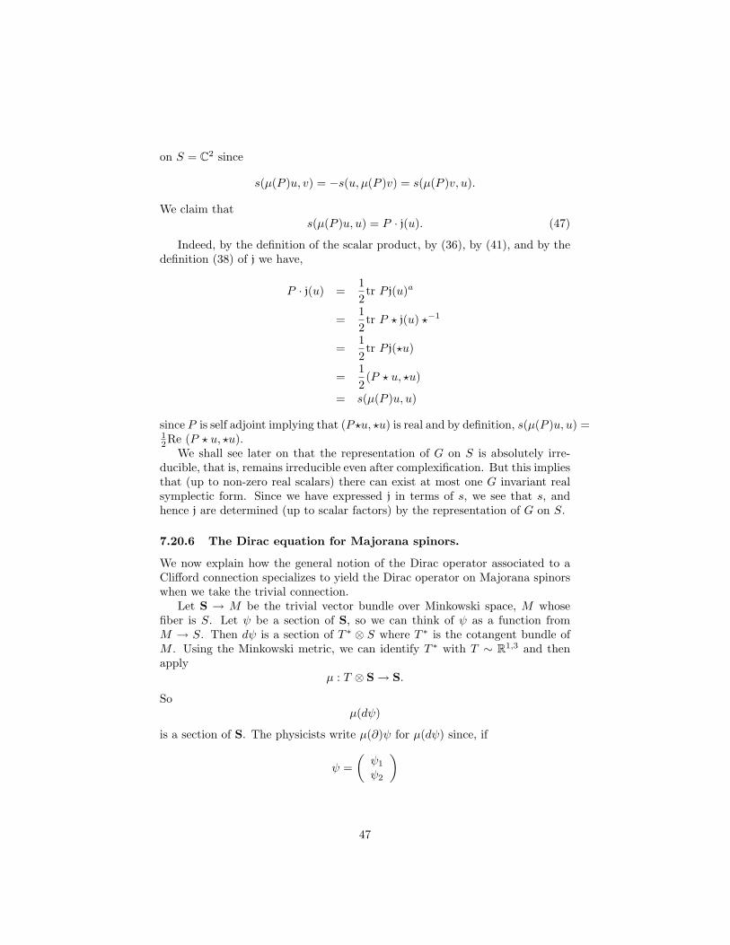
on S = C2 since
s(µ(P )u, v) = −s(u, µ(P )v) = s(µ(P )v, u).
We claim thats(µ(P )u, u) = P · j(u). (47)
Indeed, by the definition of the scalar product, by (36), by (41), and by thedefinition (38) of j we have,
P · j(u) =12
tr P j(u)a
=12
tr P ? j(u) ?−1
=12
tr P j(?u)
=12
(P ? u, ?u)
= s(µ(P )u, u)
since P is self adjoint implying that (P?u, ?u) is real and by definition, s(µ(P )u, u) =12Re (P ? u, ?u).
We shall see later on that the representation of G on S is absolutely irre-ducible, that is, remains irreducible even after complexification. But this impliesthat (up to non-zero real scalars) there can exist at most one G invariant realsymplectic form. Since we have expressed j in terms of s, we see that s, andhence j are determined (up to scalar factors) by the representation of G on S.
7.20.6 The Dirac equation for Majorana spinors.
We now explain how the general notion of the Dirac operator associated to aClifford connection specializes to yield the Dirac operator on Majorana spinorswhen we take the trivial connection.
Let S → M be the trivial vector bundle over Minkowski space, M whosefiber is S. Let ψ be a section of S, so we can think of ψ as a function fromM → S. Then dψ is a section of T ∗ ⊗ S where T ∗ is the cotangent bundle ofM . Using the Minkowski metric, we can identify T ∗ with T ∼ R1,3 and thenapply
µ : T ⊗ S→ S.
Soµ(dψ)
is a section of S. The physicists write µ(∂)ψ for µ(dψ) since, if
ψ =(ψ1
ψ2
)
47

is regarded as a C2 valued function, then
µ(dψ) =(
∂0 − ∂3 ∂1 + i∂2
∂1 − i∂2 ∂0 + ∂3
)?
(ψ1
ψ2
).
The (Majorana version of the) Dirac equation is
µ(dψ) = mψ. (48)
If ψ is a solution of this equation, the corresponding vector field, j(ψ) is calledthe current associated to ψ. We claim that
div j(ψ) = 0. (49)
Indeed
div j(ψ) := ∂ · j(ψ)
=12
tr (∂)a(ψ ⊗ ψ†)
= −12
tr ? (∂) ? (ψ ⊗ ψ†)
= −12
tr ? µ(∂)ψ ⊗ ψ†
= −12m(?ψ, ψ)
= 0.
Equation (49) expresses the “conservation of the current”.Notice that if we seek plane wave solutions to the Dirac equation
ψ(x) = cos(P · x+ α)u u ∈ C2
then (48) implies that||P ||2 = m2
if u 6= 0.We may think of d mapping sections of S to sections of T ∗ ⊗ S as defining
a flat connection on S. We may modify this connection by considering S as aU(1) bundle which has its own connection adding a one form and so considerthe equation
µ(dψ + eA⊗ ψ) = mψ.
This is the Dirac equation in the presence of an external electromagnetic fieldwith four potential A.
7.20.7 Complexifying a vector space with a complex structure.
The space of Dirac spinors is the complexification of the space of Majoranaspinors. This will involve us several times in the painful process of complex-ifying a real vector space with a complex structure, so we review the generalconstruction.
48

Let V be a real vector space with a complex structure. That is, we are givenan operator J on V such that J2 = −I. Any operator, A, on V extends as theoperator A⊗ id on V C = V ⊗C. When there is no danger of confusion we shallcontinue to denote this extended operator by A. Thus the (extended) operatorJ has eigenvalues ±i on V C. In other words V C decomposes as
V C = V C+ ⊕ V C
−
whereV C
+ := u− iJu, u ∈ V consists of all the +i eigenvectors of J and
V C− : u+ iJu, u ∈ V
consists of all the −i eigenvectors of J.Suppose that the operator Ais J linear, meaning that AJ = JA. Suppose
that we choose a J basis of V . This means that we choose vectors e1, . . . , en sothat the vectors
e1, . . . , en,Je1, . . . ,Jen
form a basis of V . Relative to such a basis the assertion that A is J linearamounts to saying that A has the block matrix decomposition
A =(a −bb a
).
Now e1 − iJe1, . . . , en − iJen is a basis of V C+ while e1 + iJe1, . . . , en + iJen is a
basis of V C− . It then follows immediately that in terms of the combined basis of
V C we have
A⊗ id =(a+ ib 0
0 a− ib
)if A =
(a −bb a
)is J linear.
Now suppose that A is anti-J linear, meaning that AJ = −JA. This amountsto saying that A has the block decomposition
A =(a bb −a
)and it follows that
A =(
0 a+ iba− ib 0
)if A =
(a bb −a
)is J anti-linear.
For example, let us consider the case where V = g is a Lie algebra in whichthe Lie bracket is J linear. This Lie bracket extends by complexification tog⊗C = gC, and the two subspaces gC
+ and gC− are subalgebras each isomorphic
to g under the isomorphisms
ξ 7→ 1√2
(ξ − iJξ), ξ 7→ 1√2
(ξ + iJξ).
49

Suppose that the Lie algebra g has a representation on the vector space Swhich carries a complex structure, JS , and that the complex structure on g isconsistent with the complex structure on S in the sense that
ξ(JSu) = (Jgξ)u.
where Jg denotes the complex structure on g. We can drop the two subscriptsand write this as
ξJu = Jξu.
Then(ξ − iJξ)(u+ iJu) = ξu+ iJξu− iJξu− i2J2ξu = 0.
In other words gC+ acts trivially on SC
− and similarly gC− acts trivially on SC
+.Also the action of gC
+ on SC+ is isomorphic to the action of g on S and similarly
for the other component.In the case of interest to us we see that
sl(2,C)⊗ C = sl(2,C)⊕ sl(2,C)
and that the space of Dirac spinors, the complexification of the space of Majo-rana spinors, decomposes as
S ⊗ C = SC+ ⊕ SC
− = (12, 0)⊕ (0,
12
),
where 12 denotes the standard two dimensional representation of sl(2,C) and 0
denotes the trivial representation.Any J− antilinear map of S (where J is now γ) extends to a complex linear
map ofD := S ⊗ C
which switches the two components. In particular this applies to the operator?. So we see that the group G acts irreducibly on D as claimed above.
Let us now consider the action of the real Lie algebra sl(2,C) on Minkowskispace, identified, as usual, with the space of self adjoint two by two matrices.The action is given by
P 7→ ξP + Pξ†.
Since every complex square matrix can be written as P + iQ where P andQ are self adjoint, we see that the complexification of Minkowski space is justgl(2,C), the space of all complex two by two matrices. Furthermore, recallingthat the complex structure on sl(2,C) is exactly multiplication by the scalarmatrix, iI, we see that
(Jξ)P = iξP = ξ(iP )
as two by two matrices and hence
(ξ + iJξ)P = 0.
50

SimilarlyP (ξ† − iJξ†) = 0.
Thus MC is irreducible under sl(2,C)⊗ C and is the representation ( 12 ,
12 ), the
tensor product of the basic representation of each factor. Recall that D = S⊗Cis the complexification of the space of Majorana spinors. We extend µ(P ) bycomplex linearity to D and define
γ(P ) = iµ(P )
where i is now the good old fashioned complex number and so commutes withµ(P ). Hence
γ(P )2 = ||P ||2I.
These are the defining relations for the Dirac “matrices”. But notice that theClifford algebra C(1, 3) is isomorphic to the algebra H(2) of all two by twomatrices over the quaternions. Hence its minimal module must have dimensioneight over the real numbers. Thus the Dirac matrices have no realization asfour by four real matrices. This is in contrast to the algebra C(3, 1) which westudied above in conjunction with the Majorana spinors. The Dirac equation isas before, namely
−iγ(∂)ψ = µ(∂)ψ = mψ.
But now ψ is a D valued function and D is a complex vector space so we canseek plane wave solutions of the form
ψ(x) = u(P )eiP ·x.
Then we must haveγ(P )u(P ) = mu(P )
which implies||P ||2 = m2
as before.Thus if ψ is a general solution of the Dirac equation, its Fourier transform
must be supported on the two sheeted hyperboloid ||P ||2 = m2. It is a factthat the space of ψ concentrated on the forward (or backward) sheet providesan irreducible unitary representation of the Poincare group.
7.20.8 Sesquilinear covariants for Dirac spinors.
For each of the bilinear covariants defined on the space of Majorana spinors Swe have a choice: we can extend it as a bilinear or as a sesquilinear form onD ⊗D. For example, let us extend j so as to be sesquilinear. Then
j(u+ iv) = (u+ iv)⊗ (u† − iv†)= u⊗ u† + v ⊗ v† + i[v ⊗ u† − u⊗ v†],
51

where u and v are elements of S. The original group G acts as real lineartransformations on D = SC and hence the relations
j(Aw) = Aj(w)A†, j(?w) = j(w)a
continue to hold for w ∈ D and A ∈ Sl(2, C). Also µ(∂) is a real operator, soif ψ is a complex (i.e. D valued) solution of the Dirac equation we continue tohave
div j(ψ) = 0.
Notice that
tr j(u+ iv) = ||u||2 + ||v||2 + 2iIm (u, v)≥ ||u||2 + ||v||2 − 2||u||||v||≥ 0.
Similarly the real symplectic form s extends to D as a C valued anti Her-mitian form:
s(v, u) = −s(u, v).
So we can define a G invariant Hermitian form by
〈u, v〉 := is(u, v). (50)
Since the complexification of any (real two dimensional) Lagrangian subspaceof S will be a null space for 〈 , 〉 we see that 〈 , 〉 has signature (2, 2). In factwe have the decomposition
D = D+ ⊕D−
into two complex inequivalent irreducible representations of sl(2,C) accordingto the ±i eigenvectors of J. The restriction of 〈 , 〉 to each component must betrivial since C2 admits no sl(2,C) invariant Hermitian form. We can see thisdirectly since
s(Ju, v) = s(u,Jv)
andJ2 = −I
imply that
s(u+ iJu, v + iJv) = s(u, v) + s(Ju,Jv) + i[s(Ju, v)− s(u,Jv)]= 0.
Notice that
〈γ(P )u, v〉 = −s(?(P )u, v)= s(u, ?(P )v)= 〈u, γ(P )v〉.
52

In other words the operators γ(P ) are self adjointrelative to the Hermitianform 〈 , 〉. It follows from equation (47) that
P · j(w) = 〈γ(P )w,w〉. (51)
The Hermitian form 〈 , 〉 determines an antilinear map D→ D∗. The imageof a spinor w is called the spinor adjoint to w and is denoted in the physicsliterature by putting a bar over w. Thus
w(z) = 〈z, w〉.
8 Special representations of sl(m/n).
8.1 The definition of the Lie superalgebras sl(m/n).
We begin by recalling the definition of these superalgebras. For general factsabout Lie superalgebras we refer to the book [Sch79] or the articles [CNS75] or[Kac77].
LetV = V0 ⊕ V1
be a supervector space with
dimV0 = m, and dimV1 = n.
The Lie superalgebra sl(V0/V1) is the (commutator) Lie superalgebra of thesuperalgebra of all endomorphisms with supertrace zero. A typical such endo-morphism has the form (
A BC D
)trA = trD.
Here
A ∈ Hom(V0, V0), B ∈ Hom(V1, V0), C ∈ Hom(V0, V1),D ∈ Hom(V1, V1).
Recall that those endomorphisms which preserve the grading (those with B =C = 0) are “even”, i.e. belong to sl(V0/V1)0 and those that reverse the grading(those with A = D = 0) are “odd”, i.e. belong to sl(V0/V1)1. We are assumingthat the vector spaces V0 and V1 are finite dimensional. The structure of theLie algebra clearly depends only on the dimensions of these spaces and hencethe notation sl(m/n).
Since our spaces are finite dimensional, we may identify Hom(V1, V0) withV0 ⊗ V ∗1 . Under this identification, if v ∈ V0 and ξ ∈ V ∗1 then v ⊗ ξ is identifiedwith the rank one linear transformation given by
(v ⊗ ξ)w = 〈ξ, w〉v
53

where 〈ξ, w〉 denotes the value of the linear function ξ on the vector w. Theserank one linear transformations span Hom(V1, V0). Similar identifications willbe made for each of the other three spaces corresponding to the entries of ourblock matrix. For example, we compute the (super)commutator[(
0 v ⊗ ξ0 0
),
(0 0
x⊗ µ 0
)]=(〈ξ, x〉v ⊗ µ 0
0 〈µ, v〉x⊗ ξ
).
Notice that the trace of the upper left block and the lower right block are bothequal to 〈ξ, x〉·〈µ, v〉. This proves that sl(V0, V1) is indeed a Lie super subalgebraof the Lie superalgebra of End(V ).
To save space we will write the above bracket relations (and similar ones) asfollows: We write
sl(V0/V1)0 = (V0 ⊗ V ∗0 )⊕ (V1 ⊗ V ∗1 )
andsl(V0/V1)1 = (V0 ⊗ V ∗1 )⊕ (V1 ⊗ V ∗0 ).
Then we would write the preceding bracket relation as
[v ⊗ ξ, x⊗ µ] = 〈ξ, x〉v ⊗ µ ⊕ 〈µ, v〉x⊗ ξ.
8.2 The representation of sl(V0/V1) on the super exterioralgebra of V .
By definition, the super exterior algebra∧
(V ) of a superspace V is∧(V ) := ∧(V0)⊗ S(V1)
where S(V1) denotes the symmetric algebra of V1 so
S(V1) =∞⊕k=0
Sk(V1)
and Sk(V1) consists of homogeneous polynomials of degree k on V ∗1 . The multi-plication in S(V1) is the ordinary multiplication of polynomials so the elementsof Sk(V1) are all declared to have even grading even if k is odd.
The Lie superalgebra sl(V0, V1) has a natural representation on∧
(V ). Per-haps the best way to realize this representation is by imbedding sl(V0, V1) in theorthosymplectic algebra as the centralizer of a one dimensional subalgebra. This“Howe pair” point of view is explained by Howe in his original paper [H77]. In[NS82] we used this description in conjunction with the method of dimensionalreduction. But here is a direct description:
Each x ∈ V1 defines a multiplication operator on S(V ):
mx : Sk(V1)→ Sk+1(V1)
54

given by(mxf)(η); = 〈η, x〉f(η), ∀ η ∈ V ∗1 . (52)
Each ξ ∈ V ∗1 defines a derivation Dξ of S(V1) so
Dξ(fg) = (Dξf)g + fDξg
determined by
Dξ1 = 0 and Dξx = 〈ξ, x〉 ∀ x ∈ V1 = S1(V1). (53)
The standard Fock commutation relations hold, i.e.
Dξmx −mxDξ = 〈ξ, x〉id. (54)
Similarly, each v ∈ V0 determines the operator of exterior multiplication byv which we currently denote by ev and each µ ∈ V ∗0 defines the operator on∧(V0) of interior multiplication by µ which we will denote by iµ. So iµ is the(odd) derivation of ∧(V0):
iµ : ∧k(V0)→ ∧k−1(V0)
determined by
iµ(ω1 ∧ ω2) = iµ(ω1) ∧ ω2 + (−1)|ω1|ω1 ∧ iµ(ω2)
on homogeneous elements,
iµv = 〈µ, v〉 ∀ v ∈ V0 = ∧1(V0),
andiµ1 = 0.
We have the supercommutation relations
[ev1 , ev2 ] = 0,[iµ1 , iµ2 ] = 0,
[ev, iµ] = 〈µ, v〉id.
In short, m and D are Bose-Einstein creation and annihilation operators whilee and i are Fermi-Dirac creation and annihilation operators.
If x ∈ V1 and ξ ∈ V ∗1 then mx Dξ is again a derivation of S(V1) since aderivation followed by a multiplication is again a derivation. In fact, it is thederivation determined by the map
y 7→ 〈ξ, y〉x
on V1 and this is just the linear transformation x ⊗ ξ. Similarly, ev iµ is thederivation of ∧(V0) determined by the linear transformation v ⊗ µ on V0.
55
If v ∈ V0 and ξ ∈ V ∗1 then ev Dξ := (ev ⊗ 1) (1⊗Dξ) is an odd derivationof∧
(V ):(ev Dξ)(σ ⊗ f) = v ∧ σ ⊗Dξf
so that
ev Dξ ((σ ⊗ f)(ω ⊗ g)) = ev Dξ(σ ∧ ω ⊗ fg)= v ∧ σ ∧ ω ⊗Dξ(fg)= v ∧ σ ∧ ω ⊗ ((Dξf)g + fDξg)
= v ∧ σ ∧ ω ⊗ (Dξf)g + (−1)|σ|σ ∧ v ∧ ω ⊗ fDξg
= (ev Dξ(σ ⊗ f))(ω ⊗ g)
+(−1)|σ⊗f |(σ ⊗ f)ev Dξ(ω ⊗ g).
By definition
ev Dξ : ∧p(V0)⊗ Sk(V1)→ ∧p+1(V0)⊗ Sk−1(V1). (55)
Similarly we have the odd derivation mx iµ on∧
(V ) and
mx iµ : ∧p(V0)⊗ Sk(V1)→ ∧p−1(V0)⊗ Sk+1(V1). (56)
Also we have the even derivations mx Dξ and ev iµ which preserve allbidegrees. We have
[ev1 Dξ1 , ev2 Dξ2 ] = ev1 Dξ1 ev2 Dξ2 + ev2 Dξ2 ev1 Dξ1
= (ev1ev2 + ev2ev1)⊗Dξ1Dξ2 since Dξ2Dξ1 = Dξ1Dξ2
= 0
and similarly[mx1 iµ1 ,mx2 iµ2 ] = 0
while
[ev Dξ, iµ mx] = ev iµ ⊗Dξ mx + iµ ev ⊗mx Dξ
= 〈ξ, x〉ev iµ ⊗ 1 + ev iµ ⊗mxDξ − ev iµ ⊗mx Dξ + 〈µ, v〉1⊗mxDξ
= 〈ξ, x〉ev iµ ⊗ 1 + 〈µ, v〉1⊗mxDξ.
This shows that sl(V0/V1) acts as derivations of∧
(V ) where
v ⊗ µ 7→ ev iµ (57)x⊗ ξ 7→ mx Dξ (58)v ⊗ ξ 7→ ev Dξ (59)x⊗ µ 7→ mx iµ. (60)
Notice that for each integer k the finite dimensional subspace of∧
(V ) given by
∧0(V0)⊗ Sk(V1)⊕ ∧1(V0)⊗ Sk−1(V1)⊕ · · · ⊕ ∧n(V0)⊗ Sk−n(V1)
56

is invariant. In the above expression (and in contrast to our notation in the nextsection) the space S`(V1) is taken to be 0 if ` < 0. It is clear that each suchsubspace is irreducible under sl(V0, V1). We have thus associated an irreduciblerepresentation of sl(V0, V1) to each non-negative integer k.
If we replace the spaces of homogenous polynomials Sk(V1) by the spacesF b of all smooth functions homogenous of degree b and defined on some fixedopen cone in V ∗1 with vertex at the origin (vertex not included), then we stillhave the multiplication operator mx : F b → F b+1 given by (52), the derivationoperator Dξ : F b → F b−1 given by (53) and the commutation relations (54)continue to hold. If dim V1 > 1 and the cone is non-empty these spaces areinfinite dimensional. But if V1 is one dimensional something special happens.
8.3 Special representations of sl(m/1).
We suppose that V1 = C. We now let Sb = Sb(V1) denote the one dimensionalspace with basis element pb. Now b can be any complex number. For x ∈ V1
definemx : Sb → Sb+1
bymxpb = xpb+1. (61)
For ξ ∈ V ∗1 defineDξ : Sb → Sb−1
byDξpb = bξpb−1. (62)
The commutation relation (54) continues to hold (where 〈ξ, x〉 is simply theproduct ξx). So the ingredients that we needed to construct the representationsof sl(m/n) in the preceding section are all present. In this way, [NS80], we haveassociated a finite dimensional representation of sl(m/1) on
∧0(V0)⊗ Sb ⊕ ∧1(V0)⊗ Sb−1 ⊕ · · · ⊕ ∧m(V0)⊗Sb−m (63)
for each complex number b and these representations are irreducible unless bis a non-negative integer with 0 < b < m. Since all the spaces Sa are onedimensional, all of these representation are on a space of dimension 2m, thesame dimension as that of the exterior algebra.
Each of the summands in (63) is invariant and irreducible under sl(m/1)0. Itwill be useful for future computations to record the action of a diagonal matrixon each of these components: The action of the diagonal matrix
u1 0 · · · 00 u2 · · · 0...
... · · ·... 0
0 0 · · · um 00 0 · · · 0 U
, U = u1 + u2 + · · ·+ um
57

is as follows:On the one dimensional space ∧0(V0)⊗ Sb it is multiplication by
bU.
If v1, . . . vm is the basis in terms of which the above matrix is diagonal, theaction on ∧1(V0) ⊗ Sb−1 is diagonal with basis v1 ⊗ pb−1, . . . , vm ⊗ pb−1 witheigenvalues
u1 + (b− 1)U, . . . , um + (b− 1)U,
and in general, the action on ∧q(V0)⊗ Sb−q is diagonal with basis
(vi1 ∧ · · · ∧ viq )⊗ pb−q, i1 < · · · < iq (64)
and corresponding eigenvalues
ui1 + · · ·+ uiq + (b− q)U. (65)
In tabulating computations we will usually use some shorthand for the eigen-vectors (64). For example we do not need to include the ⊗pb−q since this isdetermined by the representation. We will also shorten the notation for thewedge product and simply write
i1i2 . . . iq
for the eigenvector (64).
9 sl(2/1) and the electroweak isospins and hy-percharges.
In [NS80] we showed how to derive the various values of the weak isospin andhypercharge by choosing the appropriate elements of sl(2/1) and then choosingvarious parameters for b in (63). In particular, we predicted the existence of theright handed neutrino which occurs with weak isospin and hypercharge zero,and does not participate to first order in the weak interaction. With the recentdiscovery that the neutrino has positive mass [Fu98] this expectation has beenjustified.
The choice of the weak isospin and hyperchange elements of sl(2/1) are (upto the pervasive factor of i):
I3 =
12 0 00 − 1
2 00 0 0
, Y =
1 0 00 1 00 0 2
. (66)
We will tabulate below the weak isospin and hypercharge values correspond-ing to the leptons (b = 0) and the quarks (b = 2
3 ) and their anti-particles (b = 1corresponding to the anti-leptons and b = 1
3 corresponding to the anti-quarks).
58

In the full geometrical theory, we would take the tensor product of the superbun-dle associated to these representations su(2/1) with the bundle of Dirac spinorswhich has the Z2 gradation according to chirality. From the tables below it willfollow that all the particles have the same total degree (in the tensor product)which is opposite to the total degrees of the anti-particles.
9.1 b = 0 - the leptons.
We get the lepton assignments by choosing the parameter b = 0 in (63). Forthe reader’s convenience we have also tabulated the electric charge
Q = I3 +12Y.
leptons (b = 0) ∧0(V0) ∧1(V0) ∧2(V0)basis elements ∅ 1 2 12
I3 0 12 − 1
2 0Y 0 −1 − 1 −2Q 0 0 − 1 −1
particle νR νL eL eR
(67)
Notice that the gradation of the superspace on which the representation takesplace corresponds to chirality - the first and third columns which correspond to∧+(V0) = ∧0(V0)⊗S0⊕∧2(V0)⊗S−2 corresponds to right handed particles while∧−(V0) = ∧1(V0) ⊗ S−1 corresponds to left handed particles. Notice also thatthe entire even subalgebra sl(2/1)0 acts trivially on ∧0(V0)⊗ S0 correspondingto the right handed neutrino.
9.2 b = 23
- the quarks.
The choice b = 23 gives the electroweak isospin and hypercharge assignments for
quarks:quarks (b = 2
3 ) ∧0(V0) ∧1(V0) ∧2(V0)basis elements ∅ 1 2 12
I3 0 12 − 1
2 0
Y 43
13
13 − 2
3
Q 23
23 − 1
3 − 13
particle uR uL dL dR
(68)
Once again observe the relation between the gradation and chirality
59

9.3 b = 1 - the anti-leptons.
The choice b = 1 gives the anti-lepton assignment:
anti-leptons (b = 0) ∧0(V)) ∧1(V0) ∧2(V0)basis elements ∅ 1 2 12
I3 0 12 − 1
2 0Y 2 1 1 0Q 1 1 0 0
particle (eR)L (eL)R (νL)R (νR)L
(69)
Again there is a correspondence between gradation and chirality (the oppositefrom that of the leptons). Notice again that the entire even subalgebra actstrivially on ∧2.
9.4 b = 13
- the anti-quarks.
Finally the choice b = 13 gives the anti-quark assignment:
anti-quarks (b = 13 ) ∧0(V0) ∧1(V0) ∧2(V0)
basis elements ∅ 1 2 12
I3 0 12 − 1
2 0
Y 23 − 1
3 − 13 − 4
3
Q 13
13 − 2
3 − 23
particle (dR)L (dL)R (uL)R (uR)L
(70)
10 Using sl(m/1) for m = 3, 5, and 5 + n.
10.1 m = 3 - unifying quarks and leptons.
We showed in [NS80] that if we take
I3 =
12 0 0 00 − 1
2 0 00 0 0 00 0 0 0
, Y =
13 0 0 00 1
3 0 00 0 2
3 00 0 0 4
3
(71)
then we get the correct isospins and hypercharges if we combine the anti-leptonsand quarks into the single eight dimensional representation of sl(3/1) with b = 2
3and if we combine the leptons and anti-quarks in the single eight dimensionalrepresentation with b = 1
2 . We refer to [NS80] for details.
60

10.2 m = 5 - including color.
We showed in [NS80] that if we choose
I3 =
12 0 0 0 0 00 1
2 0 0 0 00 0 0 0 0 00 0 0 0 0 00 0 0 0 0 00 0 0 0 0 0
, Y =
0 0 0 0 0 00 0 0 0 0 00 0 1
3 0 0 00 0 0 1
3 0 00 0 0 0 1
3 00 0 0 0 0 1
(72)
then the single 32 dimensional representation given by
b = 2
gives the correct isospin and hypercharge assignments to the right and lefthanded up and down quarks in three colors and the right and left handed elec-trons and neutrino (so 16 in all) and their antiparticles (yielding 32). Again thechirality and the gradation match up: All the elements of ∧+ have eigenvaluescorresponding to left handed particles and all the elements of ∧− have eigenval-ues corresponding to right handed particles We refer to the Appendix in [NS80]for the list of all 32 eigenvalues.
There is something special about the value b = m−12 (for example the value
b = 2 in our current case of m = 5. Indeed, as pointed out in the note addedin proof in [NS80], the space ∧m(V0) ⊗ S−1 is acted on trivially by the evenpart of sl(m/1), i.e. has a canonical trivialization. This means that the naturalmultiplication (
∧k ⊗ Sb−k)⊗(∧m−k ⊗ Sb−m+k
)→ ∧m ⊗ S2b−m
can be thought of as invariant bilinear form on the space of the representationcorresponding to b = m−1
2 . Notice that the particles and the anti-particles ofany given species occur in the components ∧k and ∧5−kin the representation. Ifm is odd then either k or m−k is even, so the above bilinear form is symmetric.
In this set up all the particles and anti-particles have the same total tensordegree. What the meaning of the opposite total degree is in this formulation(whether “ghosts” or some other meaning) was left open to speculation.
10.3 m = 5 + n - accomodating 2n generations.
It was shown in [NS80] that generational symmetry can be achieved if we enlargethe superalgebra sl(5/1) to sl(5 + n/1). This would be a theory with 2n or2n+1 generations . At the time, this seemed inappropriate since the number ofgenerations was observed to be at least three, and was thought to be less thanfour based on arguments from the Z width. In [NS91] it was argued that if theneutrinos had positive mass, especially if the neutrinos in the higher generationswere heavy, then a fourth generation is not excluded.
61

The idea is that the weak isospin su(2) and the color su(3) are regarded ascommuting subalgebras of the even part of sl(m/1) where m = 5 + n while thegenerational behavior is produced by an sl(n/1) sub Lie superalgebra.
The I3 assignment for sl(5 + n/1) is the diagonal matrix
diag(12,−1
2, 0, . . . , 0|0) (n+ 4) zeros in all
while the hypercharge assignment is
Y = diag(−n
4 + n,−n
4 + n,
(4
4 + n
)n times
,
(4− 2n
3(4 + n)
)3 times
∣∣∣∣ 44 + n
). (73)
and the preferred representation is given by b = 5+n−12 .
We will discuss the model with four generations in the next two sections.
11 sl(7/1) - unifying color and four generations.
In this section we show how the value b = 3 can accommodate four generationsof particles with the correct isospin and hypercharge values provided that wereverse the chirality assignments in two out of the four generations. Our fun-damental superbundle will be the tensor product of the spin bundle with thebundle associated to this 128 dimensional representation. So this means thatall particles will correspond to the same total degree as indicated above. Thetables here follow the tables (42)-(45) in [NS91]. We need a name (or at least aletter) for the particles in the fourth generation, and we have tentatively chosenσ for the analogue of the electron and x and y for the analogue of the u and dquark. Also, we have made the choice that ∧0 ⊗ S3 has left handed chirality.This then determines that all the spaces with ∧k ⊗ S3−k are
left handed when k is even and are right handed when k is odd. In [NS80]the choice of m = 7 was made in order to accommodate the possibility of ghostfields. An assignment of particles without ghosts and which fits better with thetheory of Clifford superconnections will be presented in the next section.
As usual, the element I3 is given by
12 0 0 0 0 0 0 00 − 1
2 0 0 0 0 0 00 0 0 0 0 0 0 00 0 0 0 0 0 0 00 0 0 0 0 0 0 00 0 0 0 0 0 0 00 0 0 0 0 0 0 00 0 0 0 0 0 0 0
.
62

In accordance with (73) the hypercharge is given by
− 13 0 0 0 0 0 0 0
0 − 13 0 0 0 0 0 0
0 0 23 0 0 0 0 0
0 0 0 23 0 0 0 0
0 0 0 0 0 0 0 00 0 0 0 0 0 0 00 0 0 0 0 0 0 00 0 0 0 0 0 0 2
3
. (74)
Then the eigenvalues on ∧k(V0)⊗ Sb−k (and particle assignments) are given asfollows:
∧0 ⊗ S3 ∅Y 2I3 0
particle (eR)L
∧1 ⊗ S2 1 2 3 4 5 6 7Y 1 1 2 2 4
343
43
I312 − 1
2 0 0 0 0 0particle (eL)R (νeL)R (µL)R (τL)R uR uR uR
Notice the opposite chirality assignments (as compared to the electron) to the µand τ . This is somewhat arbitrary at the moment. We could make this oppositeassignment to the third and fourth generation as opposed to the second andthird.
In the next tables we will conjoin the color entries, so write 2;5,6,7 instead ofhaving three columns f25, f26, f27.
∧2 ⊗ S112 13 14 1:5,6,7 23 24 2;5,6,7 34 3;5,6,7 4;5,6,7 56,57,67
Y 0 1 1 13 1 1 1
3 2 43
43
23
I3 0 12
12
12 − 1
2 − 12 − 1
2 0 0 0 0
particle (νeR)L (µR)L (τR)L uL (νµR)L (ντR)L dL (σR)L cL tL (dR)L
63

All 35 particle assignments in the next table of eigenvalues for ∧3 ⊗ S0 areright handed. To save space we no longer indicate this in the table.
∧3 ⊗ S0123 124 12;5,6,7 134 13;5,6,7 14;5,6,7 1;56,67,67 234 23:5,6,7 24;5,6,7 2;56,57,67
Y 0 0 − 23 1 1
313 − 1
3 1 13
13 − 1
3
I3 0 0 0 12
12
12
12 − 1
2 − 12 − 1
2 − 12
part. ντL νσR yR σL cR tR yL νσLsR bR xL
∧3 ⊗ S034:5,6,7 3:56,57,67 4,56,57,67 567
Y 43
23
23 0
I3 0 0 0 0
particle xR sL bL νµL
The particles in the remaining four components of our 128 dimensional rep-resentation will be the anti-particles of the ones we have already seen, and pairedwith them under the bilinear form. So the 35 dimensional component ∧4⊗S−1
gives following table of left handed particles:
∧4 ⊗ S−11234 123;5,6,7 124:5,6,7 12;56,57,67 134;5,6,7 13:56,57,67 14;56,57,67 1567
Y 0 − 23 − 2
3 − 43
13 − 1
3 − 13 −1
I3 0 0 0 0 12
12
12
12
particle νµL bL sL xR xL bR sR νσL
∧4 ⊗ S−1234;5,6,7 23;56.57,57 24;56,57,67 2567 34;56,57,67 3567 4567
Y 13 − 1
3 − 13 −1 2
3 0 0I3 − 1
2 − 12 − 1
2 − 12 0 0 0
particle yL tR cR σL yR νσR ντL
The 21 dimensional component ∧5 ⊗ S−2 gives the following table of righthanded particles:
64

∧5 ⊗ S−21234;5,6,7 123:56,57,67 124;56,57,67 12567 134:56,57,67 13567 14567
Y − 23 − 4
3 − 43 −2 − 1
3 −1 −1I3 0 0 0 0 1
212
12
particle dR tL cL σR dL ντR νµR
∧5 ⊗ S−2234;56,57,67 23567 24567 34567
Y − 13 −1 −1 0
I3 − 12 − 1
2 − 12 0
particle uL τR µR νeR
The 7 dimensional component ∧6 ⊗ S−3 gives the following table of lefthanded particles:
∧6 ⊗ S−31234;56,57,67 123567 124567 134567 234567
Y − 43 −2 −2 −1 −1
I3 0 0 0 12 − 1
2particle uR τL µL νeL eL
Finally there is the one dimensional ∧7⊗S−4 giving the right handed particle
∧7 ⊗ S−41234567
Y −2I3 0
particle eR
12 sl(6/1).
If ghosts are not required, we use sl(6/1) to accommodate four generations:For sl(6/1) we have b = 5
2
I3 = diag(12,−1
2, 0, 0, 0, 0
∣∣∣∣ 0)
and
Y = diag(−15,−1
5,
45,
215,
215,
215
∣∣∣∣ 45
).
We will assign both left and right handed spinors to each subrepresentationso that we get four families of particles with both even and odd total gradings:
65

∧0 ⊗ S 52 ∅
Y 2I3 0
particle (L) eRparticle (R) τL
∧1 ⊗ S 32 1 2 3 4, 5, 6
Y 1 1 2 43
I312 − 1
2 0 0particle (R) eL νeL µL uRparticle (L) τR ντR σR cL
∧2 ⊗ S 12 12 13 1; 4, 5, 6 23 2; 4, 5, 6 3; 4, 5, 6 45, 46, 56
Y 0 1 13 1 1
343
23
I3 0 12
12 − 1
2 − 12 0 0
particle (L) νeR µR uL νµR dL tL dRparticle (R) ντL σL cR νσL sR xR sL
∧3 ⊗ S− 12 123 12;4,5,6 13;4,5,6 1;45,46,56 23:4,5,6 2;45,46,56 3,45,46,56 456
Y 0 − 23
13 − 1
313 − 1
323 0
I3 0 0 12
12 − 1
2 − 12 0 0
particle (R) νσR yR tR yL bR xL bL νµLparticle (L) νµL bL xL bR yL tR yR νσR
∧4 ⊗ S− 32 123;4,5,6 12;45,46,56 13;45,46,56 1456 23:45,46,56 2456 3456
Y − 23 − 4
3 − 13 −1 − 1
3 −1 0I3 0 0 1
212 − 1
2 − 12 0
particle (L) sL xR sR νσL cR σL ντLparticle (R) dR tL dL νµR uL µR νeR
∧5 ⊗ S− 52 123;45,46,56 12456 13456 23456
Y − 43 −2 −1 −1
I3 0 0 12 − 1
2particle (R) cL σR ντR τRparticle (L) uR µL νeL eL
∧6 ⊗ S− 72 123456
Y −2I3 0
particle (L) τLparticle (R) eR
66

Notice that the relation between these assignments and those of the preced-ing section are
∧07 = L∧0
6,
∧17 = R ∧0
6 ⊕ R∧16,
∧27 = L ∧1
6 ⊕ L∧26,
etc.
13 Hermitian Lie algebras.
In this section we explain the notion of a Hermitian Lie algebra which wasintroduced in [SW78] and which we used above to determine the metric on theHiggs field.
13.1 The Lie superalgebra su(2/1) and the Lie algebrasu(3).
We illustrate the notion by the relevant example. It is the special case of section2A of [SW78] corresponding to the case k = 0, ` = 2, a = 0, b = 1 of that section.
For
z =
0 0 z10 0 z2−z1 −z2 0
, w =
0 0 w1
0 0 w2
−w1 −w2 0
we let
H(z, w) = izw,
and this equals
i
−z1w1 −z1w2 0−z2w1 −z2w2 0
0 0 −w1z1 − w2z2
= i
(−z ⊗ w† 0
0 −〈z, w〉
).
The right hand side is an element of gl(2,C)⊕ gl(1,C).If we are given a hermitian form on Cn we define the complex conjugation
on gl(n,C) to beξ 7→ ξ∗ := −ξ†
where ξ† denotes the adjoint of ξ relative to the hermitian form. Then the “realsubspace”, i.e. the set of matricies fixed by this complex conjugation is u(n).
On gl(2,C)⊕gl(1,C) we put the standard complex structure on gl(2,C) butthe conjugate complex structure on gl(1,C). This means that we can write
H(z, w) = −iz ⊗ w† ⊕ i〈z, w〉1.
ThenH(z, w)∗ = −iw ⊗ z† ⊕ i〈w, z〉1 = H(w, z).
67

So H(z, w) is a hermitian form with values in the complexification of u(2)⊕u(1)and satisfies
H(w, z) = H(z, w)∗. (75)
Since commutator is a derivation of multiplication (of matrices) we have [M, zw] =[M, z]w + z[M,w] so if we define the action of ξ ∈ u(2) ⊕ u(1) on the space ofz’s to be commutator we have
[ξ,H(z, w)] = H(ξz, w) +H(z.ξw), ξ ∈ g0, z, w ∈ V (76)
whereg0 = u(2)⊕ u(1)
and whereV ∼ C2
denotes the set of all matrices of the form 0 0 z10 0 z2−z1 −z2 0
.
Explicitly, [(A 00 B
),
(0 z−z† 0
)]=(
0 Az −Bz−(Az −Bz)† 0
).
We can write this more simply as an action on C2:(A 00 B
)z = Az −Bz, z =
(z1z2
).
SoH(u, v)w = −i〈w, v〉u+ i〈v, u〉w.
Therefore if we take the cyclic sum we get zero:
H(u, v)w +H(v, w)u+H(w, u)v = 0. (77)
Now
2 ImH(z, w) =1i[H(z, w)−H(z, w)∗] =
1i[H(z, w) +H(w, z)†]
=(−z ⊗ w† + w ⊗ z† 0
0 −〈z, w〉+ 〈w, z〉
)
=
0 0 z10 0 z2−z1 −z2 0
,
0 0 w1
0 0 w2
−w1 −w2 0
.68

Thus if we define g0 := u(2)⊕u(1) and g1 = V = C2 then 2 ImH makes g0⊕g1
into the Lie algebra u(3).On the other hand,
2ReH(z, w) = H(z, w) +H(w, z)∗ = H(z, w) +H(w, z) = i(zw + wz)
is i times the anti-commutator of z and w. Since z and w are skew-adjoint theiranti-commutator is self-adjoint, so multiplying by i gives a skew-adjoint matrix.So ReH makes g0 ⊕ g1 into the super Lie algebra u(2/1).
13.2 The general definition.
So the general definition of a Hermitian Lie algebra is as follows: We startwith a real Lie algebra g0 which is represented on a complex vector space g1.We let gC
0 = g0 ⊗ C which is a complex Lie algebra with a preferred complexconjugation w 7→ w∗ so that g0 consists of the real subspace, i.e. those w whichare fixed under this complex conjugation. We assume that there is sesquilinearmap
H : g1 × g1 → gC0
which satisfies (75), (76), and (77). For the convenience of the reader we collectthese conditions here:
• (75): H is Hermitian - H(w, z) = H(z, w)∗.
• (76): H is equivariant - [ξ,H(z, w)] = H(ξz, w) + H(z.ξw), ξ ∈g0, z, w ∈ g1, and
• (77): Complex Jacobi - H(u, v)w +H(v, w)u+H(w, u)v = 0.
When this happens we make g0 ⊕ g1 into an ordinary Lie algebra using theimaginary part of H as the Lie bracket of two elements of g1, and we makeg0 ⊕ g1 into a Lie superalgebra using the real part of H as the superbracket oftwo elements of g1.
It is this relation between Lie algebras and Lie superalgebras that we use tofix the metric on the Higgs field regarded as sections of a bundle associated tog1.
13.3 The unitary algebras.
Let m = k+ ` be integers and let V0 be an m-dimensional complex vector spaceendowed with a (pseudo) Hermitian form of signature (`, k). For example wemight take
V0 = Ck,`
be complex m space with the Hermitian form
〈z, w〉 = −∑
j = 1kzjwj +m∑
j=k+1
zjwj .
69

Let c = a + b be integers and V1 a c-dimensional vector space with a (pseudo)Hermitian form of signature (b, a). Put the direct sum Hermitian on V = V0⊕V1.Then
g = u(V ),
the unitary algebra of V is an ordinary Lie algebra. Then we have the vectorspace decomposition
g = g0 ⊕ g1
where g0 is the subalgebra
g0 = u(V0)⊕ u(V1)
and g1 can be identified with the complex vector space HomC(V1, V0). (see[SW78] section 2). Then there is a structure of a Hermitian Lie algebra ong0 ⊕ g1 whose imaginary part gives u(V0 ⊕ V1).
The real part gives a class of Lie superalgebras which are called Hermitiansuperalgebras in [SS85]. They can be viewed as a real form of the complexLie superalgebra gl(V0/V1). If write the most general element of gl(V0/V1) =End(V )0 where V = V0 ⊕ V1 in the block form as(
A 00 D
)then the condition to belong to our Hermitian superalgebra is that
A ∈ u(V0) and D ∈ u(V1).
If we write the most general element of End(V )1 as(0 BC 0
)then the condition to belong to our superalgebra is
〈Cv0, v1〉1 = i〈v0, Bv1〉0 ∀ v0 ∈ V0, v1 ∈ V1.
See [SS85] page 4.
13.4 su(2, 2/1) and the superconformal superalgebra of Wessand Zumino.
The supersymmetry studied in this paper is purely internal and related to thechirality gradation as we have seen. So it is not of the “superspace” variety.Nevertheless we should point out that the superalgebra su(2, 2/1) is nothingother than the superalgebra of Wess and Zumino [CNS75] and [GGRS83] wherethe odd part of the superalgebra is regarded as the “square root” of the con-formal algebra of flat space time. We follow the presentation in [SW75] and[SS85].
70
Let V0 = C2,2 be four dimenisonal complex space equipped with a Hermitianform of signature (2, 2). To fix the Ideas let us assume that the form is given by
〈z, w〉 = w†(
0 II 0
)z = z1w3 + z2w4 + z3w1 + z4w2
where I is the two by two identity matrix.The condition that a four by four matrix A belongs to u(V0) is that
A
(0 II 0
)= −
(0 II 0
)A†.
If we break A up into blocks of two by two matrices we see that the conditionis that A be of the form (
X PQ −X†
)where X is an arbitrary complex two by two matrix and where P = −P † andQ = −Q†.
The fifteen dimensional algebra su(2, 2) is known to be isomorphic to theconformal algebra o(2, 4). Under the above description of the matrix A, thecondition to belong to su(2, 2) is that ImtrX = 0. We can regard matrices ofthe form (
0 P0 0
), P = −P †
as consisting of translations, and we may denote the set of all such matrices asg2. We can regard the matrices of the form(
0 0Q 0
), Q = −Q†
as consisting of those conformal vector fields whose expression is purely quadraticat a specified choice of origin and denote the set of such elements as g−2. Theset of elements of su(2, 2/1) of the form X 0 0
0 −X† 00 0 2iIm tr X
will be denoted by g0. If we impose the additional condition that trA = 0which is the same as Im trX = 0 we get an element of su(2, 2) which acts asa linear conformal vector field on space time, i.e. as an infinitesimal Lorentztranformation plus a scale transformation. The purely imaginary scalar matricesact trivially on space time but non-trivially on the odd part of the superalgebrawhich can be identified with the space of Dirac spinors.
The full algebra su(2, 2/1) consists of matrices of the form X P uQ −X† viv† iu† 2iIm trJ
, P = −P †, Q = −Q†, u ∈ C2, v ∈ C2. (78)
71

If X ∈ sl(2,C) then X 0 00 −X† 00 0 0
,
0 0 u0 0 viv† iu† 0
=
0 0 Xu0 0 −X†v
−iv†X iu†X† 0
.
We see that u transforms as u 7→ Xu and v transforms as v 7→ −X†v.So we have a Z gradation more refined than the Z2 gradation:
g0 = g−2 ⊕ g0 ⊕ g2
andg1 = g−1 ⊕ g1
is identified with the right and left handed spinors. We refer to [SS85] for details.
14 Renormalization of the supergroup couplingsand the Higgs mass.
For couplings given solely by the internal supergroup, i.e. by the quotientsu(2/1)/[su(2)⊗ u(1)], there is no known non-renormalization theorem. Thesecouplings are θW and a, the coefficient of the quartic. In the sequel, we showthat unitarity is preserved by appropriate BRST equations, so that we can applythe renormalization group (RG)equations to estimate the corrections. We followa linearized treatment as an approximation [HLN96] .
In one case – the angle θW – we have the group value (sinθW )2 = 0.25and may compare it to the experimentally observed value 0.229 ± 0.005. Thesupergroup prediction fits, but only very roughly. One therefore evaluates theenergy level q2 = Es at which the fit becomes precise, finding Es ∼ 5TeV. Thismay possibly be the level at which a larger symmetry structure breaks down,with SU(2/1) as the residual internal supersymmetry.
One can now invert the procedure, to estimate the renormalization effectsfor the Higgs potential quartic coefficient a. The supergroup value is assumedto hold at the energy Es = 5TeV and one then evaluates the correction fora at E ∼ 100GeV. This corrected value can then be used to reevaluate thepredicted Higgs mass, i.e. obtain the value of that mass after the inclusion ofrenormalization effects.
The coefficients of the renormalization group equation depend only on thefield contents of the theory, which is the same as in SU(2)×U(1). One cantherefore apply the Standard Model calculation. For the gauge couplings, therenormalization group equations are given by [HLN96];
1[gi(M)]2
− 1[gi(M0)]2
+ 2ti lnM
M0, i = 1, 2, 3, (79)
72
where
t1 =1
12π2(−5
3Ng −
18
),
t2 =1
12π2(−Ng −
18
+112
),
t3 =1
16π2(−4
3Ng + 11),
Ng is the number of generations, and g1, g2, g3 denote the gauge couplings ofU(1), SU(2), SU(3), respectively.For the (top-quark) Yukawa-Higgs coupling gt and the quartic Higgs couplinga, RGE are given by [SZ86];
dgtdM
=1
16π2M
92g3t − (
1712g21 +
94g22 + 8g2
3)gt
, (80)
da
dM=
116π2M
24a2 + 12ag2
t − 6g4t − 3(g2
1 + 3g22)a
+38[(g2
1 + g22)2 + 2g4
2
], (81)
These equations were solved numerically, setting the su(2/1) value of a asinitial condition holding at Es = 5TeV and taking Mt = 174GeV in The lowenergy range(E ∼ 100 to 200GeV). Assuming three generations (Ng = 3), withα−1Q = 128.80 ± .05, α−1
2 = 29.5 ± .6, α−13 = 8.332, where α−1
i = 4πg2i
and1g2Q
= 1g21
+ 1g22
In section 1.4 we discussed the mass of the Higgs field, as related to that ofthe W bosons gauging SU(2),
(M(Φ))2 =2ag2
(MW )2 = 4(MW )2, M(Φ) = 2MW (82)
In solving the equations, the relation gt(M) =√
2v Mt =
√2
246Mt was used,where v =< 0|Φ0|0 >= 246GeV . The outcome was a reduction of the predictedHiggs meson mass down to 130 ± 6GeV. Note that while there is at least oneother theory predicting the Higgs mass - ordinary supersymmetry - su(2/1)is the only one that does not require the existence of a large number of newparticles.
References
[AL73] E.S. Abers and B.W. Lee, “Gauge Theories”, Physics Reports, 9C no.1 1973
[B66] A. Berezin, The Method of Second Quantization, Academic Press, NewYork 1966
73

[Be75] Belavin, A. Polyakov, A. Schwartz and Y. Tyupkin, “Pseudo-particlesolutions of Yang-Mills equations”, Phys. Lett. 59B 85 (1975).
[BGV91] N. Berline, E. Getzler, M. Vergne: Heat Kernels and Dirac Operators,Springer, Berlin 1991
[BRS75] C. Becchi, A. Rouet and R. Stora, “Renormalization of the AbelianHiggs-model”, Comm. Math. Phys. 42 127 (1975)
[BT82] L. Beaulieu and J. Thierry-Mieg, “The Principle of BRS Symmetry:An alternative approach to Yang-Mills theories”, Nucl. Phys. B197477 (1982)
[BT83] L. Beaulieu and J. Thierry-Mieg, “Covariant Quantization of Non-Abelian Antisymmetric Tensor Gauge Theories”, Nucl. Phys. B228259 (1983)
[C94] A. Connes, Non-commutative geometry, Academic Press, New York1994
[Coq] R. Coquereaux, “Higgs fields and Superconnections”, Lecture Notes inPhysics 375
[CL90] A. Connes and J. Lott, “Particle models and noncommutative geome-try”, Nucl. Phy. 18B (Proc. Suppl.) 29 (1990)
[CNS75] L. Corwin, Y. Ne’eman, S. Sternberg, “Graded Lie algebras in math-ematics and physics”, Rev. Mod. Phy. 47 573 (1975)
[CF75] G. Curci and R. Ferrari, “A Canonical and Lorentz-Covariant Quan-tization of Yang-Mills Theories” Nuovo Cimento A 30 155-168 (1975)
[D92] A. Derdzinski, Geometry of the standard model, Springer, Berlin 1992
[DW67] B.S. DeWitt, “Quantum Theory of Gravity. II. The Manifestly Covari-ant Theory”, Phys. Rev. 162 1195 (1967)
[DiKi02] S. Dimopoulos and D.E. Kaplan, “The Weak Mixing angle from SU(3)symmetry at a TEV”, (2002) hep-ph/0201148S. Dimopoulos, D.E. Kaplan and N. Weiner, “Electroweak Unificationinto a five dimensional SU(3) at a TEV”, (2002) hep-ph/0202136
[DJ79] P.H. Dondi and P.D. Jarvis, “A supersymmetric Weinberg-Salammodel”, Physics Letters 84B Erratum 87B 403 (1979)
[DJ80] P. Dondi and P.D. Jarvis, “Assignments in Strong, Electroweak uni-fied models with an internal and space-time symmetry” (1980) Zs.furPhysik C4 201.
[Ein21] A. Einstein, “On a reasonable extension of the basis of general relativ-ity” Preuss Akad. 261 (1921)
74

[F78] D.B. Fairlie, “Two consistent calculations of the Weinberg angle”, J.Phys G. 5 L55-L58 (1978)
[F79] D.B. Fairlie, “Higgs Fields and the Determination of the WeinbergAngle”, Phys. Lett. B82 97 (1979)
[FM80] P. Forgacs and N. Manton, “Space-time symmetries in Gauge Theo-ries”, Comm. Math. Phys. 72 15 (1980)
[FP67] L.D. Faddeev and V.N. Popov, “Feynman Diagrams for the Yang-MillsField”, Phys. Lett. B25 29 (1967)
[Fu98] Y. Fukuda et al., “Constraints on neutrino oscillation parametersfrom the measurement of day-night solar neutrino fluxes at Super-Kamionkande”, Phys. Rev. Lett. 82 1810 (1999)
[GGRS83] Gates, Grisaru, Rocek and Siegel, Superspace; Frontiers in PhysicsLecture Notes Series 58 Benjamin Cummings 1983
[G78] W. Greub, Multilinear algebra Springer, Berlin (1978)
[GN63] H. Goldberg and Y. Ne’eman, “Baryon Charge and R-Inversion in theOctet Model”, Nuovo Cimento 27 1-5 (1963). Also pub. as Israel AECReport 1A-725 (February 1962)
[GL71] T.A. Golfand and E.P. Likhtman, “Extension of the algebras ofPoincare group generators P-invariance”, J.E.T.P. Lett. 13 322-326(1971)
[Hi64] P.W. Higgs, “Broken Symmetries, Massless Particles and GaugeFields”, Phys. Lett. 12 132 (1964)
[HMMN95] F.W. Hehl, J. Dermott McCrea, E.W. Mielke and Y. Ne’eman,“Metric-Affine Gauge Theory of Gravity: Field Equations, NoetherIdentities, World Spinors, and Breaking of Dilation Invariance”, inPhysics Reports (Elsevier) 258 1-171 (1995)
[H77] R. Howe, “Remarks on classical invariant theory”, preprint 1977
[HLN96] D.S. Hwang, C.Y. Lee and Y. Ne’eman, “BRST Quantizatin ofSU(2/1) Electroweak Theory in the Superconnection Approach and theHiggs Meson Mass” Intern. Jour. Mod. Phys. A11 3509-3522 (1996)
[IO96] B. Iochum and T. Schucker, “Yang-Mills-Higgs versus Connes Lott”,Comm. Math. Phys. 178 1-26 (1996)
[Kac77] V. Kac, “Lie superalgebras”, Advances in mathematics, 26 8 (1977)
[Kane93] G. Kane, Modern elementary particle physics, Perseus Publishing,Cambridge, Mass. 1993
75

[KS93] D. Kastler and T. Schucker, “A detailed account of Alain Connes’version of the Standard Model I and II”, Rev. Math. Phys. 5 477(1993)
[KS96] D. Kastler and T. Schucker, “A detailed account of Alain Connes’version of the Standard Model III and IV”, Rev. Math. Phys. 8 103,205-228 (1996)
[Li73] H.J. Lipkin, “Quarks for Pedestrians”, Phys. Reports 8C 175-263(1973)
[LN90] C.-Y. Lee and Y. Ne’eman, “Renormalization of Gauge-Affine Grav-ity”, Physics Letters B242 59-63 (1990)
[Lo27a] F. London, “Die Theorie von Weyl und die Quantenmechanik”, Natur-wiss. 15 187.
[Lo27b] F. London, “Quantenmechanische Deutung der Theorie von Weyl,”Zeit. fur Physik 42, 375-389 (1927)
[Loh78] M.A. Lohe, “Magnetic Monopoles and Backlund Transformations”,Nucl. Phys. B 142 36 (1978).
[Mai91] L. Maiani, in Proceedings of the NATO Advanced Study Institute on Z0
Physics, Cargese 1990, ed. M. Levy et al. (Plenum Press, New York,1991).
[MaSa2000] L. Mangiarotti and G. Sardanashvily, Connections in Classical andQuantum Filed Theory, World Scientific, Singapore (2000)
[MQ86] V. Mathai, D. Quillen, “Superconnections, Thom Classes, and Equiv-ariant Differential Forms”, Topology 25, 85 (1986)
[N61] Y. Ne’eman, “Derivation of Strong Interactions from a Gauge Invari-ance”, Nucl. Phys. 26 (1961) p. 222-229. Reprinted in The EightfoldWay, p. 58 (in coll. with M. Gell-Mann) “Frontiers in Physics” series,W. A. Benjamin, New York, 1964
[N64] Y. Ne’eman, “Algebraic Theory of Particle Physics”, Frontiers inPhysics Series, W. A. Benjamin, New York, 1964, 334 pp.
[N79a] Y. Ne’eman, “Ghost Fields, BRS and Extended Supergravity as Appli-cations of Gauge Geometry”, Proc. XIX Intern. Conf. on High EnergyPhysics (Tokyo 1978) Phys. Soc. Japan, 552 (1979)
[N79b] Y. Ne’eman, “Irreducible Gauge Theory of a Consolidated Salam-Weinberg Model”, Phys. Lett. B81, 190 (1979)
[N80] Y. Ne’eman, “Gauge Theory Ghosts and Unitarity - Progress in theGeometrical Treatment”, in Group Theoretical Methods in Physics,Proc. Cocoyoc (Mexico 1980), Springer Verlag Lecture Notes inPhysics 15 594 (1980)
76

[N86] Y. Ne’eman, “Internal supergroup prediction for the Goldstone-Higgsparticle mass”, Physics Letters B 181, 308 (1986)
[N95] Y. Ne’eman, “Internal Supersymmetry, Superconnections and NCG”,in Group Theory and its Applications, Proc. XXXth ELAF (Latin-American School of Physics, Mexico 1995) AIP Press no. 365 311(1996)
[N98] Y. Ne’eman, “A Superconnection for Riemannian Gravity as Sponta-neously Broken SL(4,R) Gauge Theory”, Physics Letters B427 (1998)19-25.
[N04] Y. Ne’eman, “Mathematics, Physics and Ping Pong”, Award speech forthe proceedings of the Marcel Grossman 10th, held in Rio de Janeiro,Brazil. 15 July 2003.
[NRT78] Y. Ne’eman, T. Regge and J. Thierry-Mieg, “Models of ExtendedSupergravity as Gauge Theories on Group Manifolds”, Abstract forXIX Intern. Conf. on High Energy Physics, (Tokyo, 1978).
[NS80] Y. Ne’eman, S. Sternberg, “Internal supersymmetry and unification”,Proc. Nat. Acad. Sci. USA 77, 3127 (1980)
[NS82] Y. Ne’eman, S. Sternberg, “Internal supersymmetry and dimensionalreduction”, in Gauge theories: fundamental ineractions and rigorousresults, eds. P. Dita, V. Georgescu, and R. Purice, 103 Birkhauser,Boston 1982
[NS88] Y. Ne’eman and Dj. Sijacki, “Gravity from Symmetry Breakdown ofa Gauge Affine Theory”, Phys. Lett. B200 489-494 (1988)
[NS90] Y. Ne’eman, S. Sternberg, “Superconnections and internal supersym-metry dynamics”, Proc. Nat. Acad. Sci. USA 87 7875 (1990)
[NS91] Y. Ne’eman, S. Sternberg, “Internal Supersymmetry and Supercon-nections”, in Symplectic Geometry and Mathematical Physics, (Proc.Intern. Conf. Diff. Geom. in Physics honoring J.M. Souriau, Marseilles,1990) 326 Birrkhauser, Boston 1991
[NT80a] Y. Ne’eman and J. Thierry-Mieg, “Geometrical Gauge Theory ofGhost and Goldstone Fields and of Ghost Symmetries”, Proc. Nat.Acad. Sci., USA 77 720-723 (1980)
[NT80b] Y. Ne’eman and J. Thierry-Mieg, “Geometrical Theory of Ghost andHiggs Fields and SU(2/1)”, Proc. VIII Intern. Conf. on Group The-oretical Methods in Physics, (Kiryat Anavim 1979) Annals of IsraelPhys. Soc. 3 100-116 (1980)
[Po76] A.M. Polyakov, “Particle spectrum in quantum field theory”, J.E.T.P.Lett. 20 194 (1974)
77

[Q85] D. Quillen, “Superconnections and the Chern character”, Topology 2489 (1985)
[R98] G. Roepstorff, “Superconnections and the Higgs Field”, arXiv:hep-th/9801040 v2 9 Apr 1998
[RS99a] L. Randall and R. Sundrum, “A Large Mass Hierarchy from a smallextra Dimension”, Phys. Rev. Letters 83 3370 (1999)
[RS99b] L. Randall and R. Sundrum, “An Alternative to Compactification”,Phys. Rev. Letters 83 4690 (1999)
[Sa68] A. Salam, in Elementary Particle Theory, N. Svartholm, ed. AlmquistVerlag A.B., Stockholm (1968)
[Scheck97] F. Scheck, The Standrd Model within Non-commutative Geometry:a comparison of models hep-th/9701073
[Sch79] M. Scheunert, The theory of Lie superalgebras, Lecture Notes in Math-ematics 716 Springer, Berlin (1979)
[SN90] S. Sternberg and Y. Ne’eman, “Superconnections and Internal Super-symmetry Dynamics”, Proc. Nat. Acad. Sci. USA 87 7875-7877 (1990)
[SS85] O. Sanchez-Valenzula, S. Sternberg, “The automorphism group of aHermitian superalgebra”, Lecture notes in Mathematics 1251 1-48Springer, Berlin 1985
[SNR77] M. Scheunert, W. Nahm & V. Rittenberg, “Irreducible Representa-tions of the osp(2/1) and sp1(2/1) graded Lie algebras”, J. Math.Phys. 18 156-167 (1977)
[SW75] S. Sternberg and J. Wolf, “Charge conjugation and Segal’s cosmology”,Il Nuovo Cimento 28 253 (1975)
[SW78] S. Sternberg, J. Wolf, “Hermitian Lie algebras and metaplectic repre-sentations”, Trans. Amer. Math. Soc. 231 1 (1978)
[SZ86] A. Sirlin and R. Zucchini, “Dependence of the Higgs Coupling hMS(M)on mH and the Possible onset of New Physics”, Nucl. Phys. B266 389(1986)
[T79] J.G. Taylor, “Gauging su(n/m)”, Physics Letters 84B 79 (1979)
[TM78] J. Thierry-Mieg, These de Doctorat d’Etat (U. de Paris Sud, 1978)
[TM80] J. Thierry-Mieg, “Geometrical reinterpretation of Faddeev-Popov par-ticles and BRS transformations”, J. Math. Phys. 21 2834 (1980)
78

[TM85] J. Thierry-Mieg, “Classical Geometric Interpretation of Ghost Fieldsand Anomalies in Yang-Mills Theory and Quantum Gravity” inAnomalies, W.A. Bardeen & A.R. White, eds., 239-246, World Sci-entific, Singapore 1985
[TN80] J. Thierry-Mieg and Y. Ne’eman, “Gauge Asthenodynamics (SU2/1)(classical discussion)”, Methods in Mathematical Physics (Proc. Aixen Provence and Salamanca 1979) Lecture Notes in Mathematics 836318-348 Springer, Berlin 1980
[TMN82] J. Thierry-Mieg and Y. Ne’eman, “Exterior Gauging of an InternalSupersymmetry and SU(2/1) Quantum Asthenodynamics”, in Proc.of Nat. Acad. of Sciences, USA 79 (1982) p. 7068-7072.
[TMN82a] J. Thierry-Mieg and Y. Ne’eman, “BRS Algebra of the SU(2/1) Elec-troweak Gauge Theory”, Il Nuovo Cimento 71A (1982) p. 104-118.
[’tH79] G. ’t Hooft, “Magnetic Monopoles in Unified Gauge Theories”, Nucl.Phys. B79 276 (1974)
[Ty75] I.V. Tyutin, Lebedev Institute preprint (1975)
[Wei67] S. Weinberg, “A Model of Leptons”, Phys. Rev. Lett. 19 (1967) 1264.
[Wei71] S. Weinberg, “Physical Processes in a Convergent Theory of the Weakand Electromagnetic Interactions”, Phys. Rev. Lett. 27 1688 (1971)
[Wei75] S. Weinberg, “The U(1) problem”, Phys. Rev. D11 (1975) 3583.
[Wei96] S. Weinberg, The Quantum Theory of Fields, Cambridge U. Press(1996), vol. 2.
[Wey18] H. Weyl, Raum Zeit Materie, Springer, Berlin (1918)
[YM54] C.N. Yang and R. Mills, “Conservation of isotopic spin and isospingauge invariance,” Phys. Rev. 96 191-195 (1954)
[WY75] T.T. Wu and C.N. Yang, “Concept of nonintegrable phase factors andglobal formulation of gauge fields”, Phys. Rev. D12 3845 (1975)
79