topology optimization under stress constraints

TOPOLOGY OPTIMIZATION UNDER STRESS CONSTRAINTS

By

TAE-JOONG YU

A THESIS PRESENTED TO THE GRADUATE SCHOOL OF THE UNIVERSITY OF FLORIDA IN PARTIAL FULFILLMENT

OF THE REQUIREMENTS FOR THE DEGREE OF MASTER OF SCIENCE

UNIVERSITY OF FLORIDA

2003

Copyright 2003

by

Tae-Joong Yu

ACKNOWLEDGMENTS

This thesis would not have been completed without the help of several people to

whom I wish to express my sincere appreciation. First, I wish to express my deepest

gratitude to Dr. Ashok V. Kumar for his immense help. He is my best advisor and best

mentor. He has provided excellent guidance all the time for my studies with infinite

kindness and patience. I could never have imagined a better advisor in the world.

Jongho Lee helped me to work out all problems and questions I had about

programming in C++ and Java. He opened my eyes to the exciting world of object-

oriented programming. It became an exciting experience with his knowledge and endless

help.

I would also like to show my appreciation to other friendly and helpful lab mates:

Young-Nam Hwang and Shivakumar. They always gave me answers and academic

stimulations.

To my family in Korea, I would like to express my gratitude for their dedication,

support, and love. We have been apart for three years, but my heart was always with

them and their thoughtful help and care were driving forces for this achievement.

I would like to acknowledge my dear Korean friends in Gainesville: Kyungha and

Dongsik, Kyungmin and Sangwon, Sonho and Jawoo . Ever since we met at the Atlanta

airport on June 22, 1999, we have been through everything together in the U.S.

iii

TABLE OF CONTENTS

page

ACKNOWLEDGMENTS ................................................................................................. iii

LIST OF FIGURES ........................................................................................................... vi

ABSTRACT..................................................................................................................... viii

CHAPTER 1 INTRODUCTION ............................................................................................................1

Structural Optimization................................................................................................... 2 Objective and Motivation ............................................................................................... 3

2 STRUCTURAL OPTIMIZATION...................................................................................4

Sizing Optimization ........................................................................................................ 4 Shape Optimization......................................................................................................... 4 Topology Optimization................................................................................................... 6 Homogenization Method ................................................................................................ 7

3 TOPOLOGY OPTIMIZATION using SHAPE DENSITY FUNCTION.......................12

Shape Density Function ................................................................................................ 12 Objective Function........................................................................................................ 15 Relationship between Material Properties and Density ................................................ 16 Implementation by Finite Elements .............................................................................. 17 Solution Procedure........................................................................................................ 18

4 STRESS CONSTRAINTS..............................................................................................21

Mean Compliance ......................................................................................................... 21 Problem Formulation .................................................................................................... 23

iv

5 RESULTS .......................................................................................................................28

Effect of Material Property Density Relationship ........................................................ 28 Example 1 .............................................................................................................. 28 Example 2 .............................................................................................................. 30 Example 3 .............................................................................................................. 32

Effect of Design Space (Example 4)............................................................................. 33 Effect of Safety Factor (Example 5) ............................................................................. 35 Comparison with I-DEAS Analysis.............................................................................. 37

6 CONCLUSION...............................................................................................................40

APPENDIX COMPUTER SOURCE CODE FROM OPTIMIZATION PROGRAM.....42

LIST OF REFERENCES...................................................................................................46

BIOGRAPHICAL SKETCH .............................................................................................49

v

LIST OF FIGURES

Figure page

2-1 Structural Optimization of sizing, shape and topology ................................................6

2-2 Homogrnization. ...........................................................................................................8

2-3 Material Property as a Function of Density..................................................................9

3-1 Shape Representation .................................................................................................13

3-2 Solution Flowchart .....................................................................................................19

5-1 Example 1 ...................................................................................................................28

5-2 Example 1, When n=2, The Ratio of α/γ is 332367 ...................................................29

5-3 Example 1, When n=3, The Ratio of α/γ is 498550 ..................................................29

5-4 Example 5 ...................................................................................................................30



5-7 Example 3 ...................................................................................................................32

5-8 Example 3, When n=2 ................................................................................................33

5-9 Example 4 ...................................................................................................................33

5-10 Example 4, When the Height is 0.1m.......................................................................34



5-13 Example 5 .................................................................................................................36

5-14 Example 5, When n=2 and the Safety Factor is 1 ....................................................36

5-15 Example 5, When n=2 and the Safety Factor is 1.5 .................................................37

vi

5-16 Analysis of Example 5...............................................................................................38

5-17 Analysis of first modification of Example 5 .............................................................38

5-18 Analysis of second modification of Example 5.........................................................39

vii

Abstract of Thesis Presented to the Graduate School

of the University of Florida in Partial Fulfillment of the Requirements for the Degree of Master of Science

TOPOLOGY OPTIMIZATION UNDER STRESS CONSTRAINTS

By

Tae-Joong Yu

May 2003

Chair: Ashok V. Kumar Major Department: Mechanical and Aerospace Engineering

In this thesis, shape and topology optimization of structures subject to stress

constraints is studied. The geometry is represented using a shape density function

interpolated over quadrilateral elements. This technique allows both the shape and the

topology to be treated as a variable during the optimization process. A C++ object-

oriented finite element module was implemented to perform structural analysis and

compute stiffness matrix. The optimization module iteratively modifies the geometry by

calling the finite element module. To display the optimal shape and the stress

distribution, a Java program was implemented. Multiple objectives are used to compute

the optimal structure by simultaneously maximizing the stiffness and minimizing the

mass. Maximizing stiffness is identical to minimizing the compliance of the structures.

Therefore, the objective function to be minimized is defined as a weighted sum of the

compliance and the mass of the structure. Assuming that the stress is more or less

uniform in the optimal design, a relation between the compliance and mass can be

derived for the optimal structure. Using this relation a ratio between the weighting factors

viii

in the objective function is computed such that the stress in the structure is equal to the

design stress. It was found that by using this ratio between weight factors the optimal

structures do have almost uniform stress distribution with stress values very close to the

design stress everywhere except at stress concentrations. Due to constraints on available

space for the structure, the stress concentration often occurs at the boundaries of the

feasible domain. The stress can be reduced at these stress concentrations by using larger

safety factors and also by increasing the size of the feasible domain when possible.

ix

CHAPTER 1 INTRODUCTION

Structural topology optimization is the selection of the best configuration for the

design of structures. In the last decade, the field of structural topology optimization has

expanded significantly, successfully addressing many practical engineering problems.

Structural optimization can be defined as maximizing a certain structural property subject

to one or more structural constraints. The ability to design optimal structures allows the

minimized material usage and maximized structural properties. This results in lower

manufacturing costs, which can be passed on to the costumer as lower retail costs.

Previous research on topology optimization focused primarily on global structural

behavior such as stiffness and weight. However, to obtain a true optimum design of a

structure, stresses must be considered. For example, to obtain the optimal geometry of a

structure with the objective of minimizing compliance, usually a limit on its volume or

mass is specified as the constraint. However, it is not clear what percentage of the

material volume should be sufficient for supporting the applied loads. By using

optimization method based on such a problem formulation, a trial-and-error process

cannot be avoided if the designer really wants to select the minimum-weight optimal

design for the given domain. Furthermore, it is possible that there are areas of stress

concentration on the optimal structure.

In practical optimization problems, there exists several design criteria that must be

considered in the optimal design of structures. For example, reducing the weight and

increasing the stiffness of structure are both typical design goals in a structural design,

1

2

but these objectives conflict with each other. In order to accommodate many conflicting

design goals, the sequential application of each single objective optimization can be

considered. However, this method cannot produce an optimized solution because only a

single objective is considered in each optimization process. As a consequence, so-called

multiobjective optimization, which considers multiple objectives simultaneously, has

recently been regarded as a methodology for solving optimization problems with several

objective functions. A number of techniques and applications of multiobjective

optimization have been developed over past few years. A comprehensive overview of the

field of multiobjective optimization in mechanics was introduced by Stadler [Sta 84], and

multiobjective design optimization was applied to engineering problems, including

structural design problems, by Eschenauer et al.[Ech 90].

Structural Optimization

Structural optimization can be classified into three categories: size, shape and

topology optimization. Sizing optimization starts at a structure in which the configuration

of the structure is already defined. It seeks the optimum combination of the element size

such as length, thickness, cross-sectional area, etc. It does not involve the redefinition of

shapes of outer boundaries and inner holes of structure. For this reason, if a sub-optimal

initial topology is chosen the final optimization solution will be also be suboptimal.

Shape optimization involves varying the domain of the structure. It seeks the geometric

definition of the boundaries of outer circumference and inner holes of the structure.

Design variables in shape optimization include often the location of key points that define

a curve or some parameters that define a specific predetermined geometric shape such as

edges or boundaries. During the optimization procedure, these boundaries may be

manipulated; therefore new shape can be created. If the shape is changed significantly

3

during the optimization procedure, the structural analysis package must recreate the mesh

in order to ensure minimal element distortion. The primary disadvantage to shape

optimization is similar to that of sizing optimization. If the shape optimization is based on

a specific geometric configuration, any design that is not included in the set of the

predetermined topology will not be created during the optimization procedure. Topology

optimization aims to create the best configuration of a structure from a user-defined

configuration set that comprised all possible configuration of a structure for the design

problem. This means that new geometric boundaries, such as the boundary of an internal

hole, may appear during the optimization procedure. This allows global shape and

topology optimization so that the final optimal structure no longer depends on the initial

design.

Objective and Motivation

This thesis presents the implementation of a structural topology optimization

under stress constraint. The objective of optimization procedure is to minimize the

compliance and mass of the structure, such that the stress is not over the yield stress at

any point in the structure. The ideal optimal structure has uniform stress distribution with

the stress lower than the yield stress.

CHAPTER 2 STRUCTURAL OPTIMIZATION

Structural optimization can be classified as sizing, shape, or topology

optimization. They are classified by the design variables chosen to describe the geometry.

They may also be classified based on the particular combination of objective function and

constraints used to describe the optimization problem. The following sections give a brief

description of each type of structural optimization techniques.

Sizing Optimization

Sizing optimization starts at a structure in which the configuration of structure is

already defined, such as trusses, frames and plates [Haf 86, Haf 92, Kir 81, Mor 82]. It

seeks the optimum combination of elemental size such as length, thickness, cross-

sectional area, etc. The geometry change is very small when varying these design

variables, so it does not involve the redefinition of shapes of outer boundaries and inner

holes of a structure. One of the primary disadvantages of sizing optimization is that the

topology of the structure remains fixed throughout the optimization procedure. Therefore,

if a sub-optimal topology is chosen when formulating the optimization problem, the

resulting structure will also be sub-optimal. The optimal design of a sizing optimization is

only best design that can come out of the predetermined structural geometric definition.

Shape Optimization

Shape optimization seeks the geometric definitions of the boundaries of outer

circumference and inner holes of structure. Shape optimization requires the finite element

model to change during the optimization procedure. The design variables used for shape

4

5

optimization cause boundary variation and these are referred to as the “shape design

variables”. Compared to sizing optimization, the computational cost of shape

optimization is higher due to the need to constantly update the finite element model.

Shape optimization is divided into two categories; parametric variable variation

and boundary variation. In parametric variable variation, the design variables are

parameters defining certain features of the shape or important dimensions. For instance,

the side of a square hole or the radius of a circular hole could be a design variable. Many

examples of shape variation using parametric variables have been illustrated by Botkin et

al.[Bot 86]. In boundary variation, parts of the boundary of the solid are treated as the

design variables. For instance, the nodal coordinates of the nodes on the boundary of the

shape could be the design variables. Yang [Yan 86] showed many examples of this type

of shape optimization.

A thorough review on shape optimization methods and applications was provided

by Haftka and Grandhi [Haf 86]. The geometric configuration of a structure is required

before the shape optimization can be performed. If the shape optimization is based on a

specific geometric configuration, any design that is not included in the set of the

predetermined geometric modeling will not be created during the optimization.

Therefore, the shape optimization converges to different optimal shapes for different

starting topologies. Another drawback to shape optimization is the finite element model

must be continually updated to ensure that the mesh does not become highly distorted.

This task is difficult because mesh refinement and recreation must be performed

automatically during the optimization procedure.

6

Topology Optimization

From above sections, it was realized that to obtain optimal shapes the topology

must be modified during the optimization procedure. Early works by Dorn et al. [Dor 64]

and Dobbs and Felton [Dob 69] implemented topology optimization techniques in which

simple numerical methods were used to find optimal layout and geometry for truss. Most

topology optimization research in the next two decades was devoted to structural analysis

using the finite element method followed by removal of under-stressed element. The final

optimized shapes were highly dependent upon the density of the mesh used for the finite

element analysis. Strang [Str 86] attributed this behavior to the non-convex nature of the

problem. Kohn and Strang [Koh 86], representing that the original problem was ill posed,

proposed a relaxed variational problem, which allows composite or porous material

instead of an all-or-nothing dichotomy between material and holes. Bendsoe and Kikuchi

[Ben 88] proposed the homogenization method to determine the properties of these

composite materials.

Figure 2-1. Structural Optimization of sizing, shape and topology

7

The homogenization method is a mathematical tool for modeling the behavior of

periodic structures, such as composites or porous materials, whose properties vary

periodically at microscopic level [Ben 78]. The homogenization method has also been

successfully applied to many structural design problems [Kikuchi 93, Ben 91] in which

the objective function was the compliance of the structure with multiple-loading cases

and three-dimensional applications.

Homogenization Method

The main idea of structural topology design using homogenization method is that

a solid structural domain is modeled as a composite material with possibly perforated

microstructures. Consequently, the homogenization method is utilized to analyze the

composite structure. The behavior of periodic structure at a macroscopic level is

predicted in the limit when the Tε (the ratio of period of the structure to a typical

macroscopic length scale) tends to zero.

The early approaches to topology optimization allowed the material to either exist

in a state of full density, or not exist at all (an all-or-nothing approach). Areas void of

material shows either holes, or areas outside of the structure’s outermost boundary.

During this optimization procedure, under-stressed element will be removed. This

method may have difficult convergence problem. To overcome some of these difficulties,

Kohn and Strang [Koh 86] proposed the use of homogenization as a means of allowing a

uniform distribution of properties from 0 to 1. The difficult convergence problem

suggested the need to relax the original variational problem statement so that it would be

well-posed and have better convergence performance. Kohn and Strang showed that

relaxing the variational problem is identical to allowing composite materials for the

8

solution. By means of the homogenization method, the structural topology optimization

problem is used as the optimal material distribution problem.

By assuming the material to be porous and solving for the optimal distribution of

porosity, Bendsoe and Kikuchi [Ben 88] have elaborated on the above finding. A design

domain is defined as the space in which the structure must fit. This domain is divided into

a rectangular mesh with respect to the given boundary conditions and loads.

Figure 2-2. Homogrnization. A) Unit Cell, B) Unit Cell Orientation in an Element

The finite element method is used to analyze the structural behavior under the boundary

conditions and the applied loads. Bendsoe and Kikuchi modeled the material as porous by

assuming a specific microstructure. The material is represented as a porous medium

containing infinitely many microscale cells. Suzuki and Kikuchi [Suzuki 91] have

assumed a rectangular hole having edge dimension of ‘a’ and ‘b’ as shown in Figure 2-

2(A). The dimensions of the hole within a unit cell determine the overall porosity or hole

fraction of the material. Each finite element in the mesh is assumed to have a fixed

porosity or hole fraction associated with its own hole dimensions ‘ai’ and ‘bi’ where ‘i’ is

9

the element number. These hole dimensions along with the angular orientation of the unit

cells θ are the design variables. Initially, all elements are assumed to have the same hole

dimensions and orientation giving the material a uniform porosity.

i

To solve for the optimal porosity distribution, Bendsoe and Suzuki [Ben 88,

Suzuki 91] used an optimality criteria algorithm. The material properties are continuous

function of the hole dimensions. For a given porosity or hole size, the material properties

can be determined using the homogenization method. The relation between material

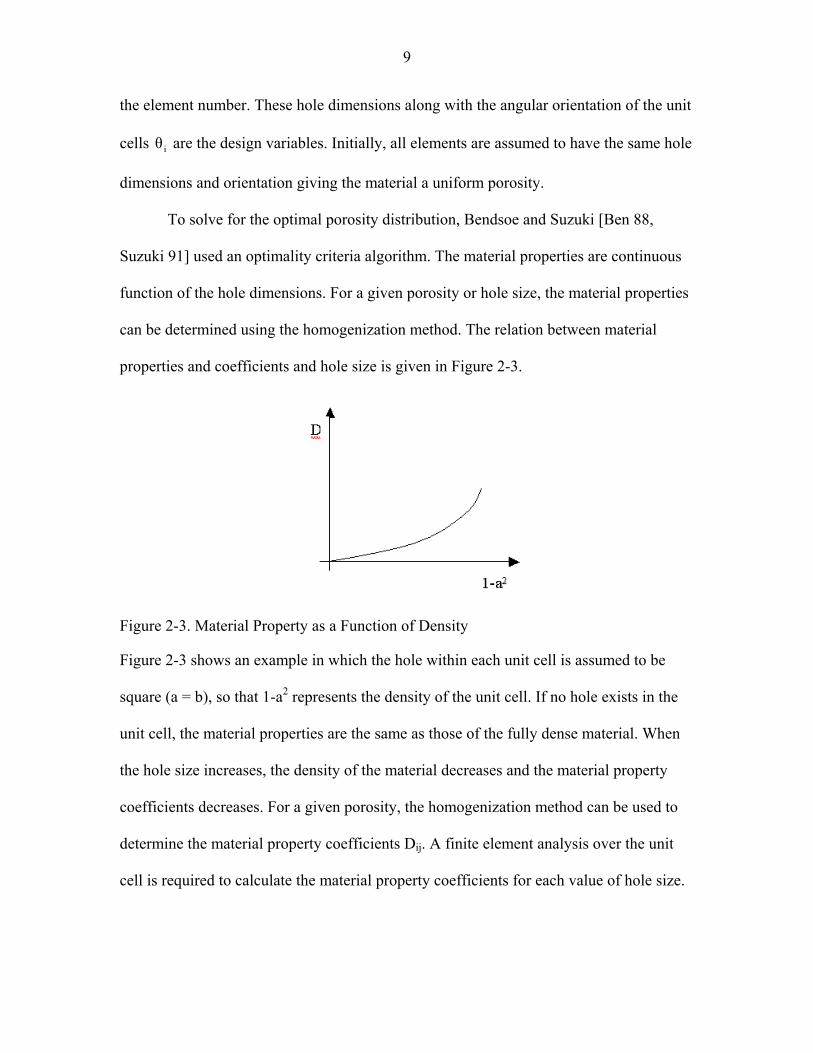
properties and coefficients and hole size is given in Figure 2-3.

Figure 2-3. Material Property as a Function of Density

Figure 2-3 shows an example in which the hole within each unit cell is assumed to be

square (a = b), so that 1-a2 represents the density of the unit cell. If no hole exists in the

unit cell, the material properties are the same as those of the fully dense material. When

the hole size increases, the density of the material decreases and the material property

coefficients decreases. For a given porosity, the homogenization method can be used to

determine the material property coefficients Dij. A finite element analysis over the unit

cell is required to calculate the material property coefficients for each value of hole size.

10

During the optimization procedure, the hole size is increased in areas where the

stresses are low, which results in low-density material. On the contrary, the hole size is

decreased in areas where material has high stresses, resulting in high-density. When

optimization procedure converges, some elements will have large hole sizes so that they

have low density and other will have zero hole size (fully dense material). Elements with

density value below a specific threshold value can be removed to reveal the final

optimized topology.

The relation between material property coefficients and hole size would be

different for different microstructures. In the method adapted by Bendsoe and Kikuchi

[Ben 88], a square or rectangular hole was assumed within a unit cell. Recently, Allaire

and Kohn [All 92] have used rank 2 microstructures. Figure 2-4(a) shows a

microstructure consisting of unit cells with rectangular holes and Figure 2-4(b) illustrates

a rank-2 microstructure. The rank-2 consists of alternating layers of stiff material and

rank-1 material. Rank-1 material in turn consists of alternating layers of stiff and soft

material. Allaire and Kohn [All 92] have demonstrated that for a composite material with

a fixed ratio of the components, the rank-2 layer yields the stiffest composite. The

optimal shape, which is solved for using rank-2 layering, does not have clearly defined

holes or boundaries. Instead, the optimal results obtained suggest that the truly optimal

structure may have continuously varying density due to continuously varying ratio of two

constituents. Since it is not economically or physically possible to control the density and

ratio of constituent within a structure, such composites are difficult to manufacture. The

geometry of the structure obtained by the above method does not yield smooth

boundaries, especially when a coarse finite element mesh is used.

11

Figure 2-4. Microstructures. A)By Microscale Rectangular, B)By Rank-2

Papalambros et al. [Pap 90] used image-processing techniques to extract a feasible initial

shape from the topology generated by the homogenization method. They then used this

shape as the starting shape for conventional shape optimization by boundary variation. A

similar two-step process has been used by Bendsoe [Ben 91] to obtain combined

topology and shape optimization.

CHAPTER 3 TOPOLOGY OPTIMIZATION USING SHAPE DENSITY FUNCTION

Shape Density Function

In order to model the geometry as a variable, we define the boundaries of the

geometry to be the contours of a density field )(xφ , which we refer to as the shape

density function. The shape density function has values in the range from a threshold

value Tφ to 1. The contours of this function corresponding to the threshold value Tφ of

density express the boundaries of the geometry. The density field is defined over a

feasible domain Ω . The shape being expressed may be defined as the subset of this

feasible domain within which the density value is greater than or equal to the threshold

value. In other words, the geometry consists of the set of

0

0Ω∈x for which

1)( ≤≤ xφφT (3-1)

Figure 3-1 shows geometry representation using a shape density function. The L shape

region shown is the feasible domain within defined geometry. The final shape must fit

within this region. The figure shows contours of the shape density function according to

constant values of densities. The fully dense regions (where 1=φ ) are shown in black

color and the white regions have density less than the threshold value. Therefore the

white regions are void of material. All other density values are represented using a

grayscale color distribution with darker shades representing higher density than lighter

shades. Representation of shape using the shape density function allows the entire

geometry to be treated as a variable, thus we can combine shape and topology

12

13

optimization. In the shape optimization procedure, the internal hole shown in the figure

would not be created if it were not included in the initial design provided by the designer.

Figure 3-1. Shape Representation

To define the shape density function within the feasible domain, the domain is divided

into a quadrilateral mesh and the nodal values of density are specified. The density

function distribution within each element is obtained by interpolating the nodal values.

Using 4-node quadrilateral elements, the density function within each element can be

expressed as,

(3-2)

where, iφ are the nodal density values and are the isoparametric shape functions

for the 4-node quadrilateral element expressed in terms of the parametric coordinates s

and t [Bathe 87]. The shape function can be expressed as

),( tsNi

),(),(),(),(),( 44332211 tsNtsNtsNtsNts φφφφφ +++=

14

)1)(1(41

1 tsN ++= , )1)(1(41

2 tsN +−=

)1)(1(41

3 tsN −−= , )1)(1(41

4 tsN −+=

For an isoparametric element, the mapping between the parametric space and the real

coordinates (x, y) is defined by

∑=

=4

1

),(i

ii tsNxx and (3-3) ∑=

=4

1

),(i

ii tsNyy

The geometry can be graphically displayed by plotting gray scale border of the density

function where different shades of gray are used for different ranges of density values.

Since a bilinear interpolation is used to represent the density distribution within each

element, the contours of the density are linear within each element. Contours are plotted

by connecting points of equal density on the edges of an element. A C0 continuous shape

density function ensures C0 continuous boundaries for the final shape, providing a means

of combined shape and topology optimization.

To have a fully dense final design, it is desirable that the density changes sharply

from the threshold value to 1 at the boundary. However, since the shape density function

is a C0 continuous function, it cannot change discontinuously from the lowest value to the

highest. The sharpest transition that can be represented is limited by the size of the

quadrilateral elements used for the piece wise interpolation of this function. The density

values can change from highest value at one end of the element to the lowest value at the

other end. Therefore, the smaller the element size the sharper the density variation can be

at the boundaries. From a purely shape representation point of view, if we define the

threshold value to be equal to or nearly equal to 1, then within the boundaries of the

geometry the material would be fully dense. However, when applying this shape

15

representation scheme for topology optimization, a lower value of threshold is desirable

so that optimal designs that are not fully dense can also be represented.

The design problem definition consists of specifying the feasible domain, the

loads the structure has to carry and the displacement boundary conditions that describe

how the structure is supported. In Figure 3-1, the arrows at the top represent a uniformly

distributed load supported by structure. The solid triangles represent nodes that are

constrained to have zero displacement.

Objective Function

For the maximum stiffness topology design, minimizing the mean compliance of

a structure is commonly used as the objective function and the constraint is imposed on a

somewhat arbitrarily chosen material volume. However, it should be noted that the

designer usually does not know what percentage of the material volume should be

sufficient for supporting applied loads. Therefore, we should consider minimizing both

the mean compliance and the mass as the objective. The design goal is to obtain the

optimal topology of a structure, which maximizes the stiffness and minimizes the mass,

which ensures that stress is lower than yield stress. Therefore, multiple objectives should

be considered. We limited the study to planar problems such as plane stress and plane

strain. The multi-objective problem may be written as

Minimize : ))(()( φγφα xLM + (3-4)

0 1≤≤ φ

where α and γ are user specified control parameters.

The mass, ),(φM can be expressed as

φA T=Ω= ∫Ω dM φφ)( , (3-5)

16

where and Ω= ∫Ω dNA φ is nodal density values

The mean compliance, , is written by )(xL

∫ ∫Ω Γ

Γ⋅+Ω⋅= ddL )()())(( φφφ xtxfx (3-6)

This mean compliance is twice the work done by the applied force (traction t and body

force f) during the displacement x. To obtain the mean compliance, we can use additional

equation,

[ ] )()( 0

0

xD δεφδε LdT

=Ω∫Ω

(3-7)

ε and δε are the strain and virtual strain in the structure caused by the displacement x

and the virtual displacement xδ respectively. [ ])(φD is the matrix of elastic constants that

relate stresses and strains for a linear elastic material. Assuming that these elastic

constants are functions of the shape density function, as the shape changes (φ changes)

the stiffness, the compliance and the deformation of the structure for the given load also

change.

The optimization problem given by the equation 3-4 through 3-7 can be solved using a

nonlinear programming algorithm. This work uses a variation of sequential programming,

which is described in Kumar and Gossard [Kum 93a] and Kumar [Kum 93b].

Relationship between Material Properties and Density

In order to affect the outcome of the finite element analysis with the shape density

function, some relationship between material properties and density has to exist. The

relation between the elastic modulus and the density has to be selected such that when

material is removed, the structure should become more compliant. When the

17

minimization of the compliance and the mass is subject to the stress constraint, the

algorithm will distribute density such that material is available in locations where it

contributes to minimizing compliance and mass. In this thesis, its relation between

material properties and density is considered as

nEE φ0= (3-8)

where, is the Young’s modulus of the material of the structure, 0E φ is the density.

Implementation by Finite Elements

The deformation of the structure and its mean compliance were computed by

finite element method. To construct the stiffness matrix, we integrate the principle of

virtual work, over each element to obtain the element stiffness matrix and then assemble

these together to obtain the global stiffness matrix. In this thesis, we have used four-node

isoparametric quadrilateral elements for the analysis. Therefore, the displacements are

represented by piece-wise bilinear interpolation within each element. This representation

yields the following strain-displacement relation for the element

[ ] eh

e uBε = (3-9)

where, [ ]

∂∂

∂∂

∂∂

∂∂

∂∂

∂∂

∂∂

∂∂

=

yN

yN

yN

yN

xN

xN

xN

xN

4321

4321

B and ehu is the displacement vector

corresponding to the quadrilateral finite element. Substituting this relation in (3-7), for

each element, we get

( ) ( )[ ] [ ] ( )[ ][ ] ehe

TTehe

eTee ududLee

Ω=Ω= ∫∫

ΩΩ

BDBDu φδεφδεδ (3-10)

18

( ) [ ] ehe

Teh

e uuL Ku δδ = , where, [ ]eK is the element stiffness and ehuδ is the virtual

displacement vector. The element stiffness matrix [ ]eK can be expressed as

[ ] [ ] ( )[ ][ ] e

T

e de

Ω= ∫Ω

BDBK φ (3-11)

Since the quadrilateral element has a bilinear interpolation for the displacement field

within each element, [B] is not a constant matrix. The terms of matrix are linear functions

of the parametric coordinates s and t. The elasticity matrix is a function of the parametric

coordinates, since it depends on the density function. The integration in Eq. (3-11) can be

calculated by using gaussian quadrature approach. Before using the gaussian quadrature

approach, we need to determine the correct order of quadrature. To get this order, the

degree of the polynomial terms of the [ ] ( )[ ][ ]BDB φT matrix must be determined. Since

density is a linear function in the parametric coordinate s and t, the terms in the matrix

are polynomials of degree 2+n (where n is the degree of the polynomial in (3-

8). Gaussian quadrature of order m (using m x m integration points) can integrate a

polynomial of degree 2m-1.

[ ] [ ][ ]BDB T

Solution Procedure

Two primary modules solve the topology optimization program; which are the

optimization module and the finite element module. The optimization module controls

the solution procedure, and calls the finite element module when the objective function is

calculated. The first step of the optimization procedure is reading an input data file. Once

the input data has been processed, the optimization module is called. The purpose of the

optimization module is to calculate the nodal density values within the design domain

19

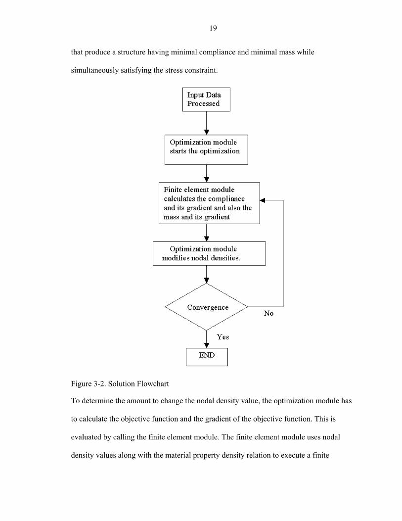
that produce a structure having minimal compliance and minimal mass while

simultaneously satisfying the stress constraint.

Figure 3-2. Solution Flowchart

To determine the amount to change the nodal density value, the optimization module has

to calculate the objective function and the gradient of the objective function. This is

evaluated by calling the finite element module. The finite element module uses nodal

density values along with the material property density relation to execute a finite

20

element analysis [Kum 00]. By the finite element analysis, the nodal displacements are

calculated. The finite element module to calculate the compliance and its gradient values

uses these nodal displacements. Then the optimization module uses these values to vary

the nodal density values, resulting in the necessity to perform another finite element

analysis. This iterative procedure continues until all convergence criteria are satisfied.

With the final nodal displacement, the stress values are calculated. These stress values

and the final density values are written to an output file to be used in the graphical

display program. Figure 3-2 illustrates a flowchart showing the solution procedure.

CHAPTER 4 STRESS CONSTRAINTS

Mean Compliance

The mean compliance is the same as twice of the total strain energy at

equilibrium. Bendsoe [Ben 88] describes its relation. The mean compliance can be

written as

∫∫ ΩΩΩ=Ω= ddL CσσDεεε TT)( (4-1)

D is the matrix of elasticity constants that relate stresses and strains for a linear elastic

material. C is the compliance matrix. When we assume that the material is isotropic, C is

given by

−−−−−−

=1

11

1

νννννν

EC , (4-2)

where ν is Poison’s ratio, E is Young’s modulus, and 321 σσσ=T

,, 21

σ is the vector

of the three principal stresses. In terms of the principal stresses σσ and 3σ , the von

Mises stress can be calculated as

( ) ( ) ( )213

232

2212

1 σσσσσσσ −+−+−=von (4-3)

A constraint on the allowable values of the von Mises stress in Ω can be expressed as

2max

2 σσ ≤= MσσTvon (4-4)

where maxσ is given maximum allowable stress and

21

22

−−

−−

−−

=

121

21

211

21

21

211

M . (4-5)

In the case of plane stress, the following relation can be obtained [Ben 88]

MσσCσσMσσ TTT )1(213

)1(21 νν−≤≤

+EE

(4-6)

Equation 4-6 shows that the von Mises stress is bounded by a multiple of the square root

of strain energy density at an arbitrary point in Ω , i.e.,

CσσT

)1(23

νσ

+≤

Evon or (4-7)

( ) ( ) )(123

123 εCσσT L

vE

vEdAσ 2

von +=

+≤ ∫∫

ΩΩ

(4-8)

Using this result, the relation between the mean compliance problems and problems in

which the stress is bounded over the design domain can be obtained. Assuming that the

stress is nearly constant and the von Mises stress is almost the same as the maximum

stress over the optimum layout, the mean compliance can be computed with the mean

stress. Therefore, Eq. 4-8 can be simplified as

)()1(2

3A2max εLE

νσ

+≤ (4-9)

where is the area (2D) of . We obtain a lower bound on the mean compliance by A Ω

A3

)1(2)( 2maxσνε

EL +

≥ (4-10)

23

Problem Formulation

Our objective is minimizing the mass and the mean compliance with stress

constraints. That is, minimize

))(()( φγφα xLM + (4-11)

(4-12) 10 ≤≤ φ

where α and γ are user specified control parameters. ),(φM the mass can be expressed

as

φA T=Ω= ∫Ω dM φφ)( ,where Ω= ∫Ω dNA (4-13)

Using the strain-displacement relation, [ ] xBε = ,assumed in FEA model, the mean

compliance equation Eq. 4-1 can be written as

[ ] [ ][ ] Ω= ∫ dL xBDBxx TT

Ω)( (4-14)

where, is the nodal displacement vector. x

We can rewrite this equation as

[ ] [ ][ ] [ ] [ ][ ][ ] xBDBxxBDBxx TTTT

Ω ∫∫ ΩΩ=Ω= ddL )( (4-15)

[ ] xKxx T=)(L , where [ is the stiffness matrix. ]K

[ ] [ ] [ ][ ]∫Ω Ω= dBDBK T (4-16)

In the objective function, when α increases the optimal mass will be decreased and when

α decreases the optimal mass will be increased. By choosing appropriate α and γ

values, minimum mass and minimum compliance with fully stressed constraint can be

obtained. Optimally, following conditions should be satisfied.

0)()( =∇+∇ xLM γφα (4-17)

24

where

AφA =∂∂

=∂∂

=∇ T

ii

MMφ

φφ

φ )()( (4-18)

[ ] [ ] [ ] [ ] [ ] iiii

Lφφφφ ∂

∂+

∂∂

+∂∂

=∂∂

=∇xKxxKxxKxxKxx TT

TT)(

(4-19)

[ ] FxK = , therefore,

[ ] ( ) 0=∂∂ xK

iφ (4-20)

[ ] [ ]

[ ] [ ] xKKx

xKxK

ii

ii

∂∂

−=∂∂

=∂∂

+∂∂

−1

0

Q

(4-21)

Substituting, Eq. 4-21 into Eq. 4-19, we obtain

[ ] xKxx T

i

Lφ∂∂

−=∇ )( (4-22)

Therefore, Eq. 4-17 can be written as

[ ] 0A =− XCX Tii γα (4-23)

where, [ ] [ ] [ ] [ ][ ] Ω∂∂

=∂∂

= ∫ dii

i BDBKCT

Ωφφ (4-24)

When we assume that stresses are uniform everywhere for the optimal solution and, then

from Eq. 4-10 we have

2*

3)1(2

)()(

*

+=

= NEML yσνφ φφ

x (4-25)

where, maxσσ

=N

y , N is safety factor and yσ is yield stress.

25

From Eq. 4-13 and Eq. 4-15 we got

[ ]

∑=

= n

iii

ML

1

A)()(

φφXKXx T

. (4-26)

At the optimal solution, from Eq. 4-23, we get

[ ] XCX Tii α

γ=A (4-27)

[ ]( ) [ ] XEXXCX Tii

Tn

iii α

γφαγφ == ∑∑

=1

A (4-28)

Hence, Eq. 4-25 can be written as

[ ] [ ]

2

3)1(2

)()(

+==

∗

= ∗ NEv

ML yσ

γα

φ φφ XEXXKXx

T

T

(4-29)

where, [ ] [ ] [ ] i

n

i ii

n

iφ

φφ KCE i ∑∑

== ∂∂

==11

(4-30)

We obtain the ratio of α and γ as

[ ] [ ]

2

3)1(2

+=

NEv yσ

γα

XKXXEX

T

T

(4-31)

If , [ ] where nEE φ0= [ ] nφ0DD =

[ ]

−−=

2100

0101

1 2ν

νν

νED and [ ]

−−=

2100

0101

1 20

0

νν

ν

νED .

Therefore, for this study we consider different polynomial material property density

relations of the form

nEE φ0= (4-32)

26

where, is the Young’s modulus of the material and 0E φ is the density and n is an

integer. Differentiating the [D] matrix with respect to the design variable

[ ] [ ] [ ] [ ] [ ] iNii

n

i

n

i

nnnφφ

φφφ

φφφφ

φ111 DDDD

00 =

∂∂

=∂∂

=∂

=∂∂ −D∂ (4-33)

Then Eq. 4-24 can be written as

[ ] [ ] [ ] [ ]dVNn i

V

BDBC Ti φ∫= (4-34)

The stiffness matrix of each element is calculated by

[ ] [ ] [ ][ ]dVV

BDBK Te ∫= (4-35)

From Eq. 4-27, [E] matrix of each element can be computed by

[ ] [ ] [ ] [ ][ ] [ ] [ ][ ] dVNnVdNnnpe

iii

V

npe

i

ii

Vi

npe

i∑∫∑∫∑===

===111

φφφ

φφ BDBBDBCE TTie (4-36)

where, npe is the number of nodes per element.

Since , Eq. 4-35 and Eq. 4-36 can be combined to obtain φφ =∑=

npe

iii N

1

[ ] [ ee KE n= ]

(4-37)

We can rewrite Eq. 4-31 by this relation:

[ ] [ ] [ ]∑∑==

==ne

eee

ne

eeee n

11XKXXEXXEX e

TTT (4-38)

where, ne is number of elements

[ ] [ ]∑=

=ne

eee

1XKXXKX e

TT , (4-39)

[ ] [ ]

n=XKXXEX

T

T

(4-40)

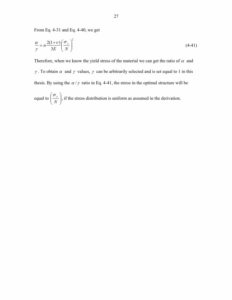
27

From Eq. 4-31 and Eq. 4-40, we get

2

3)1(2

+=

NEn yσν

γα (4-41)

Therefore, when we know the yield stress of the material we can get the ratio of α and

γ . To obtain α and γ values, γ can be arbitrarily selected and is set equal to 1 in this

thesis. By using the γα / ratio in Eq. 4-41, the stress in the optimal structure will be

equal to

, if the stress distribution is uniform as assumed in the derivation.

N

yσ

CHAPTER 5 RESULTS

Effect of Material Property Density Relationship

Example 1

The feasible region shown in Figure 5-1, whose dimensions were 0.41x0.41, was

divided into a uniform quadrilateral mesh containing 1764 nodes and 1681 elements. All

nodes on the left side edge were fixed. Uniform pressure in the X-direction was applied

on six elements in the middle of the right side edge of the domain. The applied pressure is

equal to the design stress (=200MPa) of the material. The Young’s modulus of the

material used in the structure is 2.07GPa. The Poisson’s ratio is 0.29.

Figure 5-1. Example 1

28

29

Figure 5-2. Example 1, When n=2, The Ratio of γα / is 332367


30

Figure 5-2 and Figure 5-3 show the optimal geometries and their stress distributions. The

stresses are almost uniform everywhere, with values similar to those of the design

(200MPa).

Example 2

The rectangular feasible region, whose dimensions are 0.51(h)x0.26(w) was


the nodes on the left side edge of the feasible were fixed. Uniform pressure was applied

in the Y-direction to six elements along the right side edge. The Young’s modulus of

material used in the structure is 2.07GPa. The Poisson’s ratio is 0.29. The applied

pressure is equal to the shear yield stress (=100MPa).


Figure 5-5 and 5-6 show the optimal geometries and its stress distributions. In these two

pictures, we can see the stress concentration in each corner. Except for those two regions,

the stress is almost uniform everywhere else.

31



32

The range of the stresses is 1.6MPa ~1.9MPa if the stress concentrations are ignored. The

reason of the existence of stress concentration is that the optimal geometry must fit in the

design domain. The high stress at the corners can be reduced if a larger feasible region

was available.

Example 3

The feasible region is L-shape block shown in Fig. 5-7. The feasible region was


nodes on the right side edge were fixed. Uniform pressure was applied as shown in Fig.

5-7. The Young’s modulus of material was assumed to be 2.07GPa and the Poisson’s

ratio equal to 0.29. The applied pressure is equal to the yield stress (=200MPa).


In this L-shape structure, bending moment due to the applied load is too large to be

supported by structure even if the geometry of the structure was identical to the feasible

region. In addition, there is stress concentration at the inside corner of the shape.

33

Figure 5-8. Example 3, When n=2

Therefore, it is not possible to design a structure to carry this load that can fit in the

feasible region. A valid design can be found only by enlarging the feasible domain.

Effect of Design Space (Example 4)

The design space in practical engineering design problems is often limited due to

which the topology optimization process yields structures that have stress concentration

at the boundary of the feasible region. This example investigates this by varying the

height of the initial design domain.


34

The Young’s modulus of material used in the structure is 2.07GPa and the Poisson’s ratio

is 0.29. The design domain is shown in Figure 5-9. In Figure 5-10, h equals 0.1m, in

Figure 5-11, h equals 0.2m and in Figure 5-12, h equals 0.3m. The ratio of γα / is

332367

Figure 5-10. Example 4, When the Height is 0.1m


35


When the height constraint is changed from 0.1m to 0.2m (Figure 5-10 and Figure 5-11),

its maximum stress reduces from 7.586GPa to 2.4759GPa. In Figure 5-10, there are stress

concentrations on each left side corner. In Figure 5-11, the height of the feasible region

was doubled compared to that in Figure 5-10. This means that expanding the feasible

region reduces the stress concentration. When the height increases from 0.2m to 0.3m,

there is not significant difference.

Effect of Safety Factor (Example 5)

The rectangular feasible region, whose dimensions were 0.5(h)x0.3(w), was


nodes on the left side edge were fixed. Uniform pressure was applied on the six elements

at the bottom right side corner in the y-direction. The Young’s modulus of the material

used in the structure is 2.07GPa and the Poisson’s ratio is 0.29. The applied pressure is

equal to the yield stress (=200MPa). In Figure 5-14, safety factor is 1 and the ratio of

γα / is 332367. In Figure 5-15, safety factor is 1.5 and the ratio of γα / is 147718.

36


Figure 5-14. Example 5, When n=2 and the Safety Factor is 1

Average stress = 221711304 Max Stress = 810938231

37

Figure 5-15. Example 5, When n=2 and the Safety Factor is 1.5

Average stress = 158755368 Max Stress = 548166674 When the safety factor is increased from 1 to 1.5, average stress is reduced and its

maximum stress is also reduced.

Comparison with I-DEAS Analysis

In order to verify stress distribution in the optimal structure in example 5, I-DEAS

software was used to compare the results. The optimal shape computed in Figure 5-15 is

used for the comparison. After creating the solid model in I-DEAS that is almost identical

to the result in Figure 5-15, FEA analysis was performed to obtain the stress distribution.

Figure 5-16 shows the result of the analysis. There is a stress concentration on the left

corner of the structure. The maximum stress (4.83e8 Pa) is greater than twice the yield

stress (2.00e8 Pa). The topology optimization program is unable to eliminate this stress

concentration due to the limited space available within the feasible domain.

38

Figure 5-16. Analysis of Example 5

Figure 5-17. Analysis of first modification of Example 5

39

To reduce the maximum stress, the designer has to modify the design further as shown in

Fig. 5-17. In Figure 5-17, the maximum stress was reduced to 2.91e8 Pa by adding more

material near the stress concentration. However, this maximum stress is still slightly

above the yield stress and there is stress concentration also. Figure 5-18 shows the stress

distribution after further modification. We can still see stress concentration on the right

corner, but the value of stress of this area is almost same as the yield stress.

Figure 5-18. Analysis of second modification of Example 5

CHAPTER 6 CONCLUSION

In sizing optimization, the design variables are the cross-sections of the truss or

the thickness of the plate etc. The geometry change is quite small when varying these

design variables so it is not necessary to create a new analysis model each time the design

variables are changed. This means that the topology of the structure remains fixed

throughout the optimization procedure. For this reason, designers usually use sizing

optimization after they have developed a detailed design that they wish to optimize.

Shape and topology optimization is a powerful tool that can be used in the

conceptual design phase. Since the entire geometry is considered as a variable, large

structural changes are possible such as the creation of new holes and/or boundaries.

Therefore, the optimal shape is independent of the initial guess.

An implicit shape representation is used in this thesis where the contours of a

shape function corresponding to a threshold value are treated as the boundaries of the

shape. The shape density function is defined over a feasible region and is represented by

a piece-wise linear interpolation over quadrilateral finite element. The values of the

density function at the nodes are used as the design variables. As the shape changes, the

structural properties should change also. This means that the material properties should

be related to the shape density function.

In this thesis, the implementation of structural topology optimization under stress

constraint is studied. A relation between the compliance and mass is developed for the

optimal design assuming that the stress is uniform for the optimal structure. The design

40

41

objective is to obtain the optimal topology of a structure, which maximizes the stiffness

and minimizes the mass, such that the stress distribution over the design domain is

uniform and equal to the desired design stress.

An object-oriented topology optimization program was implemented using the

C++ programming language. The program consists of two primary components, an

optimization module and a finite element module. The optimization module was adapted

from a previously developed program written by Dr. Ashok Kumar [Kum 93a]. To

display the results of optimization program, a graphical display program was used that

was originally developed by Wood [Woo 98]. This program was further modified to

display the stress distribution for this thesis.

The results in this thesis illustrate that the multiobjective optimization approach

can be used to simultaneously minimize mass and maximize stiffness such that the stress

constraints are satisfied everywhere except at stress concentration. This approach is good

for conceptual design of structures. However, the geometry of the structure thus obtained

has to be further modified by the designer to remove stress concentrations and to satisfy

other non-structural design requirements.

APPENDIX COMPUTER SOURCE CODE FROM OPTIMIZATION PROGRAM

The following source code is for calculating the objectives and their gradients.

#include <math.h> #include <stdio.h> #include <stdlib.h> #include <iostream.h> #include <fstream.h> #include <string.h> #include <time.h> #include "c1topopt.h" #include "opt.h" #include "fe_solver.h" #include "fe_model.h" #include "interpolation.h" #include "element.h" #include "a_type.h" #include "c1_4n_quad.h" double C1topopt::ALPHA=0.; double C1topopt::BETA=0.; double C1topopt::GAMMA=0.; /*================Constructor for Top_opt===================*/ C1topopt::C1topopt(int nn1,int nec1,int nic1,double *x1,double *g1, double **h1,int nsc1, double **sc1, double *hc1,double **ghc1, double *gc1,double **ggc1,ofstream out1,FE_Model *fem1, Interpolation *c1_integ1): Opt(nn1,nec1,nic1,x1,g1,h1,nsc1,sc1,hc1,ghc1,gc1,ggc1) fem=fem1; c1_integ=c1_integ1; outstream=out1; /*===============double eval_function()=====================*/ double C1topopt::eval_function() // Purpose : Returns the value of the objective function, for given x // Stores values of constraints in gc, for given x // Increment the counter num_func_calls++; double *value=new double[1]; value--; value[1]=0; int size=1; double func, func1=0.0; double func2=0.0; int tne=fem->get_tot_num_ele(); for(int i=1;i<=tne;i++) c1_integ->integration(fem,object_fn1,i,value,size); func1+=value[1];

42

43

cout << "mass = " << func1 << endl; if (BETA!=0.0) for(i=1;i<=tne;i++) c1_integ->integration(fem,object_fn2,i,value,size); func2+=value[1]; cout << "surface = " << func2 << endl; // Compute compliance FE_Solver *fes=fem->get_fes(); fes->fill_Kmax(); fes->assemble_skylineK(); fes->assemble_skylinef(); fes->skyline_solver(1); double compliance = fes->compliance(); cout<<"Current value of Compliance = "<<compliance<<endl; func = func1 + func2 + GAMMA*compliance; return func; /* end eval_function */ /*==============void set_final_compliance()=======================*/ void C1topopt::set_abc(double a, double b, double c) ALPHA = a; BETA = b; GAMMA = c; /*==================================================*/ double C1topopt::get_alpha() return ALPHA; /*==================================================*/ double C1topopt::get_beta() return BETA; /*==============void eval_grad_hess()=======================*/ double *g_mass; void C1topopt::eval_grad_hess() /* Purpose : evaluate the gradient & the Hessian of the /* of the objective fn. and gradient of the constraints /* Note: Call eval_function before calling this function */ int i,j,k; int nspn,tmp; nspn =0; int num_ele_typs=fem->get_num_ele_typs(); Element **ele=new Element *[num_ele_typs]; *ele[num_ele_typs]--; for(i=1;i<=num_ele_typs;i++) ele[i]=fem->get_ele(i); tmp = ele[i]->get_phi_interpolation()->get_num_sfs_per_node(); if(tmp>nspn) nspn = tmp; int tot_num_nds=fem->get_tot_num_nds(); int nn = nspn*tot_num_nds; //total number of design variables for (i=1;i<=nn;i++) g[i]=0.0; for (i=1;i<=num_ele_typs;i++)

44

A_Type *atyp=ele[i]->get_atyp(); double t=atyp->get_thickness(i,0.5,0.5); // Thickness Interpolation *phi_intep=ele[i]->get_phi_interpolation(); int nnpe = ele[i]->get_nds_per_ele(); int tnsfs = nnpe*nspn; // num of shape functions per element if(g_mass==NULL) g_mass = new double[tnsfs]; g_mass--; for (int i1=1;i1<=tnsfs;i1++) g_mass[i1]=0.0; for (j=1;j<=ele[i]->get_num_ele();j++) phi_intep->integration(fem,grad_object_fn,j,g_mass,tnsfs); for (k=1;k<=nnpe;k++) for (int l=1;l<=nspn;l++) int k1 = ele[i]->get_ele_con(j,k)*nspn - nspn + l ; int k2 = k*nspn - nspn + l ; g[k1]+=g_mass[k2]*t; double *grad_c; /** Note: The gradient of the function is stored as ggc in Opt **/ grad_c=fem->grad_compliance(); for(i=1;i<=nn;i++) g[i] += GAMMA*grad_c[i]; // eval_grad_hess //====================object function===================== int *con; void object_fn1(FE_Model *fem,int en,int num_sfs_per_ele, double *nx,double **dn, double *value,int size) value[1]=0.; Element *ele=fem->get_ele(1); int nds_per_ele=ele->get_nds_per_ele(); if(con==NULL) con=new int[nds_per_ele];con--; for(int j=1;j<=nds_per_ele;j++) con[j]=ele->get_ele_con(en,j); double *x=fem->get_phi(); Interpolation *c1_interp=ele->get_phi_interpolation(); int nspn=c1_interp->get_num_sfs_per_node(); // Add density to value[1] double ALPHA = C1topopt::get_alpha() ; for(int k=1;k<=nds_per_ele;k++) for(int k1=1; k1<=nspn;k1++) value[1]+=ALPHA*x[con[k]*nspn-(nspn-k1)]*nx[(k-1)*nspn+k1]; //object_fn1 void object_fn2(FE_Model *fem,int en,int num_sfs_per_ele,

45

double *nx,double **dn, double *value,int size) value[1]=0.; Element *ele=fem->get_ele(1); int nds_per_ele=ele->get_nds_per_ele(); if(con==NULL) con=new int[nds_per_ele];con--; for(int j=1;j<=nds_per_ele;j++) con[j]=ele->get_ele_con(en,j); double *x=fem->get_phi(); Interpolation *c1_interp=ele->get_phi_interpolation(); int nspn=c1_interp->get_num_sfs_per_node(); // Add laplacian of density to value[1] double BETA = C1topopt::get_beta(); for(int k=1;k<=nds_per_ele;k++) value[1]+=BETA*(x[con[k]*nspn-3]*dn[(k-1)*nspn+1][3] + x[con[k]*nspn-2]*dn[(k-1)*nspn+2][3] + x[con[k]*nspn-1]*dn[(k-1)*nspn+3][3] + x[con[k]*nspn]*dn[(k-1)*nspn+4][3] + x[con[k]*nspn-3]*dn[(k-1)*nspn+1][4] + x[con[k]*nspn-2]*dn[(k-1)*nspn+2][4] + x[con[k]*nspn-1]*dn[(k-1)*nspn+3][4] + x[con[k]*nspn]*dn[(k-1)*nspn+4][4]); //object_fn2 //====================gradient object function===================== void grad_object_fn(FE_Model *fem,int en,int nsfns, double *nx,double **dn, double *shape,int size) double ALPHA = C1topopt::get_alpha() ; double BETA = C1topopt::get_beta(); for(int i=1;i<=nsfns;i++) shape[i]=ALPHA*nx[i]+BETA*(dn[i][3]+dn[i][4]);

LIST OF REFERENCES

[All 92] Allaire, G. and Kohn, R.V., “Topology optimization and optimal shape design using homogenization,” Topology Design of Structures, Ed. M. P. Bendsoe and Mota Soares, Kluwer Academic Publisher, New York, pp. 182-194, 1992.

[Ben 92] Bendsoe, M.P., Diaz, A. and Kikuchi, N., “Topology and

generalized layout optimization of elastic structures,” Topology Design of Structures, Ed. Bendsoe and Mota Soares, Kluwer Academic Publisher, New York, pp. 238-250, 1992.

[Ben 91] Bendsoe, M.P. and Rodrigues, H.C., “Integrated topology and

boundary shape optimization of 2-D solids,” Computer Methods in Applied Mechanics and Engineering, vol. 87, pp. 15-34, 1991.

[Ben 88] Bendsoe, M.P. and Kikuchi, N., “Generating optimal topologies in

structural design using a homogenization method,” Computer Methods in Applied Mechanics and Engineering, vol. 71, pp. 197-224, 1988.

[Ben 78] Bensoussan, A., Lions, J. and Papanicolaou, G., Asymptotic

Analysis for Periodic Structures, North-Holland Publishing Company, New York, 1978.

[Bot 86] Botkin, M.E., Yang, R.J. and Bennett, J.A., “Shape optimization of

three-dimensional stamped and solid automotive components,” The Optimum Shape, J.A. Bennett and M.E. Botkin Editors, Plenum Press, New York, 1986.

[Dob 69] Dobbs, M.W. and Felton, L.P., “Optimization of truss geometry,”

Journal of Structural Engineering, vol. 95, pp. 2105-2118, 1969. [Dor 64] Dorn, W.S., Gormory, R.E. and Greenburg, H.J., “Automatic

design of optimal structures,” Journal de Mechanique, vol. 3, pp. 25-52, 1964.

[Esc 90] Eschenauer, H., Koski, J. and Osyczka, A., Multicriteria design

optimization: Procedure and applications, Berlin: Springer, 1990.

46

47

[Haf 92] Haftka, R.T. and Gurdal, Z., Elements of Structural Optimization, 3rd Edition, Kluwer Academic Publisher, New York, 1992.

[Haf 86] Haftka, R.T. and Grandhi, R.V., “Structural shape optimization –

A survey,” Computer Methods in Applied Mechanics and Engineering, vol. 57, pp. 91-106, 1986.

[Kir 81] Kirsch, U., Optimum Structural Design: Concepts, Methods and

Applications, McGraw-Hill Book Company, New York, 1981. [Koh 86] Kohn, R.V. and Strang, G., “Optimal design and relaxation of

variational problems,” Communications in Pure and Applied Mathematics, vol. 39, pp. 113-137, 139-182, 333-350, 1986.

[Kum 00] Kumar, A.V., and Yu, Lichao, “An object-oriented modular

framework for implementing the finite element method,” Computers and Structures, vol. 79, no.9, pp. 919-928, 1998.

[Kum 93a] Kumar, A.V. and Gossard, V, “Sequential approximation method

for structural optimization using logarithmic barriers,” Advances in Design Automation, American Society of Mechanical Engineering, Design Engineering Division (Publication) DE, vol. 65, pt 1, pp. 735-742, m1993.

[Kum 93b] Kumar, A.V., “Shape and topology synthesis of structures using a

sequential optimization algorithm,” Ph.D. Thesis, Massachusetts Institute of Technology, Cambridge, MA., 1993.

[Mor 82] Morris, V, “Foundations of Structural Optimization: A Unified

Approach,” John Wiley and Sons, 1982. [Pap 90] Papalambros, Panos and Chirehdast, Hehran, “An integrated

environment for structural configuration design,” Journal of Engineering Design, vol. 1, pp. 73-96, 1990.

[Sta 84] Stadler, W., “Multicriteria optimization in mechanics.” Applied

Mechanics Review, vol. 37, pp. 277-286, 1984. [Str 86] Strang, Gilbert and Kohn, R.V., “Optimal design in elasticity and

plasticity,” International Journal for Numerical Methods in Engineering, vol.22, pp. 183-188, 1986.

[Suz 91] Suzuki, K. and Kikuchi, N., “A homogenization method for shape

and topology optimization,” Computer Methods in Applied Mechanics and Engineering, vol. 93, pp. 291-318, 1991.

48

[Woo 98] Wood, A. “Shape and topology optimization using a shape density function interpolated over quadrilateral elements,” M.S. Thesis, University of Florida, Gainesville, FL, 1998.

[Yan 86] Yang, R.J., Choi, K.K. and Haug, E.J., “Numerical considerations

in structural component shape optimization,” ASME Journal of Mechanics, Transmissions and Automation in Design, vol. 107, No. 3, pp. 334-339, 1986.

BIOGRAPHICAL SKETCH

Tae-Joong Yu was born on March 3, 1971, in Seoul, Korea. He grew up in an urban

area. In spring 1991, he began an undergraduate program in the Mechanical Design and

Production Engineering Department of Kon-Kuk University. After two years of studying

in the program, he enrolled in the military service from 1992 until 1993 to fulfill his

mandatory service as a Korean citizen. After discharge, he returned to Kon-Kuk

University and graduated in spring 1998. He began his master’s degree study in fall 1999

and from summer 2000 he studied with Dr. Ashok V. Kumar in the Mechanical

Engineering Department of the University of Florida, Gainesville, Florida.

49

topology optimization under stress constraints

Documents