topological features in vector fieldsjmeyer/papers/c-26.pdf · topological features in vector...

Topological Features in Vector Fields

Thomas Wischgoll and Joerg Meyer

Electrical Engineering and Computer Science, University of California, Irvine[twischgo|jmeyer]@uci.edu

Summary. Vector fields occur in many application domains in science and engi-neering. In combustion processes, for instance, vector fields describe the flow of gases.This process can be enhanced using vector field visualization techniques. Also, windtunnel experiments can be analyzed. An example is the design of an air wing. Thewing can be optimized to create a smoother flow around it. Vector field visualiza-tion methods help the engineer to detect critical features of the flow. Consequently,feature detection methods gained great importance during the last years.

Methods based on topological features are often used to visualize vector fieldsbecause they clearly depict the structure of the vector field. Most algorithms basi-cally focus on singularities as topological features. But singularities are not the onlyfeatures that typically occur in vector fields. To integrate other features as well,this paper defines a topological feature for vector fields based upon the asymptoticbehavior of the flow. This article discusses techniques that are able to detect thisfeature.

Key words: Topological analysis, Vector field visualization, Flow visualiza-tion, Closed streamlines, Feature detection.

1 Introduction

Many of the problems in natural science and engineering involve vector fields.Fluid flows, electric and magnetic fields are nearly everywhere, therefore mea-surements and simulations of vector fields are increasing dramatically. As withother data, analysis is much slower and still needs improvement. Mathematicalmethods together with visualization can provide help in this situation. In mostcases, the scientist or engineer is interested in integral curves of the vector fieldsuch as streamlines in fluid flows or magnetic field lines. The qualitative natureof these curves can be studied with topological methods developed originallyfor dynamical systems. Especially in the area of fluid mechanics, topologicalanalysis and visualization have been used successfully [9, 13, 18, 25].

But often, topological methods cover only a few topological features thatcan occur in vector fields. Basically, only the singularities of a flow are con-sidered in most algorithms. For instance, a sink is not the only topologicalfeature that is able to attract the surrounding flow. This becomes quite ev-ident when thinking about bifurcation. Consider the Hopf bifurcation as an

2 Thomas Wischgoll and Joerg Meyer

example. There, a closed streamline may arise from a sink. This closed stream-line then has the same properties as the sink it originated from: it attracts theflow in exactly the same way. Based on this motivation, this paper defines ageneral topological feature that covers singularities such as sources and sinksbut also other features depending on their attracting or repelling property.

First, an introduction of existing vector field visualization methods is givenincluding topological techniques. Then, topological features are discussed anda clear definition of a topological feature based on asymptotic behavior of theflow is given. Subsequently, algorithms are described that are able to detectthis kind of feature. Finally, results are shown and future work is discussed.

2 Related Works

Several visualization methods for vector fields are available at present. Here,the focus is on describing those methods that are useful in this applicationarea. An overview over the various visualization methods can also be foundin other publications [10] and PhD theses [19, 26].

Topological methods depict the structure of the flow by connecting sources,sinks, and saddle singularities with separatrices. Critical points were first in-vestigated by Perry [22], Dallmann [5], Chong [4] and others. The method it-self was first introduced in visualization for two-dimensional flows by Helmanand Hesselink [12]. Several extensions to this method exist. Scheuermann etal [25] extended this method to work on a bounded region. To get the wholetopological skeleton of the vector field, points on the boundary have to betaken into account also. These points are called boundary saddles. To createa time dependent topology for two-dimensional vector fields, Helman and Hes-selink [13] use the third coordinate to represent time. This results in surfacesrepresenting the evolution of the separatrices. A similar method is proposed byTricoche et al. [27, 28] but this work focuses on tracking singularities throughtime. Although closed streamlines can act in the same way as sources or sinks,they are ignored in the considerations of Helman and Hesselink and others.

To extend this method to three-dimensional vector fields, Globus et al. [9]present a software system that is able to extract and visualize some topolog-ical aspects of three-dimensional vector fields. The various critical points arecharacterized using the eigenvalues of the Jacobian. This technique was alsosuggested by Helman and Hesselink [13]. But the whole topology of a three-dimensional flow is not yet available. There, stream-surfaces are required torepresent separatrices. A few algorithms for computing stream-surfaces ex-ist [16, 24] but are not yet integrated in a topological algorithm.

There are a few algorithms that are capable of finding closed streamlinesin dynamical systems that can be found in the numerical literature. Aprilleand Trick [2] propose a so called shooting method. There, the fixed point ofthe Poincare map is found using a numerical algorithm like Newton-Raphson.Dellnitz et al. [7] detect almost cyclic behavior. It is a stochastic approachwhere the Frobenius-Perron operator is discretized. This stochastic measureidentifies regions where trajectories stay very long. But these mathematicalmethods typically depend on continuous dynamical systems where a closedform description of the vector field is available. This is usually not the case invisualization and simulation where the data is given on a grid and interpolated

Topological Features in Vector Fields 3

inside the cells. Van Veldhuizen [29] uses the Poincare map to create a series ofpolygons approximating an attracting closed streamline. The algorithm startswith a rough approximation of the closed streamline. Every vertex is mappedby the Poincare map iteratively to get a finer approximation. Then, this seriesconverges to the closed streamline. De Leeuw et al. [6] present a simplificationmethod based on the Poincare index to simplify two-dimensional vector fields.An example is shown where a closed streamline is simplified to a single criticalpoint. Even though the method might be able to detect closed streamlines ina two-dimensional flow based on the Poincare index, it is hardly extendableto 3-D.

To get a hierarchical approach for the visualization of invariant sets, andtherefore of closed streamlines as well, Burkle et al. [3] enclose the invariantset by a set of boxes. They start with a box that surrounds the invariant setcompletely which then is successively bisected in cycling directions. The pub-lication of Guckenheimer [11] gives a detailed overview concerning invariantsets in dynamical systems.

Some publications deal with the analysis of the behavior of dynamicalsystems. Schematic drawings showing the various kinds of closed streamlinescan be found in the books of Abraham and Shaw [1]. Fischel et al. [8] presenteda case study where they applied different visualization methods to dynamicalsystems. In their applications also strange attractors, such as the Lorentzattractor, and closed streamlines occur.

Wegenkittl et al. [30] visualize higher dimensional dynamical systems. Todisplay trajectories, parallel coordinates [17] are used. A trajectory is sampledat various points in time. Then, these points are displayed in the parallelcoordinate system and a surface is extruded to connect these points. Heptinget al. [14] study invariant tori in four dimensional dynamical systems by usingsuitable projections into three dimensions to enable detailed visual analysisof the tori.

Loffelmann [19, 20] uses Poincare sections to visualize closed streamlinesand strange attractors. Poincare sections define a discrete dynamical systemof lower dimension which is easier to understand. The Poincare section whichis transverse to the closed streamline is visualized as a disk. On the disk, spotnoise is used to depict the vector field projected onto that disk. Using thismethod, it can be clearly recognized whether the flow, for instance, spiralsaround the closed streamline and is attracted or repelled or if it is a rotatingsaddle. Additionally, streamlines and stream-surfaces show the vector field inthe vicinity of the closed streamline.

3 Theory

This chapter introduces the fundamental theory which is needed for the follow-ing sections. The description mainly follows the book of Hirsch and Smale [15].

3.1 Data Structures

In most applications in scientific visualization the data is not given as a closedform solution. The same holds for vector fields. Often, a vector field results


from a simulation or an experiment where the vectors are measured. In such acase, the vectors are given at only some points of the domain of the Euclideanspace. These points are then connected by a grid. A special interpolationcomputes the vectors inside each cell of that grid. In this paper, we restrictourselves to a few types of grids, basically triangular and tetrahedral grids.Using barycentric coordinates, vectors inside the cells can be interpolatedlinearly from the vectors given at the vertices [26, 31].

3.2 Vector Field Features

From a topological point of view critical points are an important part ofvector fields. This special feature is described in more detail in this section.We start with the definition of critical points in the general case and thenclassify different types of singularities.

Definition 3.1 (Critical point)Let v : W → Rn be a vector field which is continuously differentiable. Letfurther x0 ∈W be a point where v(x) = 0. Then x0 is called a critical point,singularity, singular point, zero, or equilibrium of the vector field.

Critical points can be classified using the eigenvalues of the derivation ofthe vector field. For instance, we can identify sinks that purely attract theflow in the vicinity while sources repel it purely. A proof for this attractingrespectively repelling behavior can be found in [15].

Definition 3.2 (Sink and Source)Let v be a vector field which is continuously differentiable and x0 a criticalpoint of v. Let further Dv(x0) be the derivation of the vector field v at x0. Ifall eigenvalues of Dv(x0) have negative real parts, x0 is called a sink. If alleigenvalues of Dv(x0) have positive real parts, x0 is called a source.

Streamlines are a very intuitive way to depict the behavior of the flow.But when computing such a streamline it may occur that the streamline com-putation does not terminate. This mostly is due to closed streamlines wherethe streamline ends up in a loop that cannot be left. These closed stream-lines are introduced and explained in this section. More about the theoreticalbackground can be found in several books [34, 23].

Definition 3.3 (Closed streamline)Let v be a vector field. A closed streamline γ : R → Rn, t 7→ γ(t) is astreamline of a vector field v such that there is a t0 ∈ R with γ(t+nt0) = γ(t)∀n ∈ N and γ not constant.

3.3 General Features in Vector Fields

The topological analysis of vector fields considers the asymptotic behavior ofstreamlines. To describe this asymptotic behavior we have two different kindsof so called limit sets, the origin set or α-limit set of a streamline and the endset or ω-limit set.


Definition 3.4 (α- and ω-limit set)Let s be a streamline in a given vector field v. Then we define the α-limit setas the following set: {p ∈ Rn|∃(tn)∞n=0 ⊂ R, tn → −∞, limn→∞ s(tn) → p},while the ω-limit set is defined as follows: {p ∈ Rn|∃(tn)∞n=0 ⊂ R, tn → ∞,limn→∞ s(tn) → p}. We speak of an α- or ω-limit set L of v if there existsa streamline s in the vector field v that has L as α- or ω-limit set.

��

Fig. 1. Example for α- and ω-limit sets.

If the α- or ω-limit set of a streamline consists of only one point, thispoint is a critical point. The most common case of a α- or ω-limit set in aplanar vector field containing more than one inner point of the domain is aclosed streamline. Figure 1 shows an example for α- and ω-limit sets. Thereis one critical point and one closed streamline contained in the vector field.Both, the critical point and the closed streamline are their own α- and ω-limitset. For every other streamline the closed streamline is the ω-limit set. If thestreamline starts inside the closed streamline, the critical point is the α-limitset. Otherwise the α-limit set is empty. With these explanations, we can givea precise definition of a topological feature of a vector field.

Definition 3.5 (Topological feature)Let v be a vector field. Then, a topological feature of v is an α- or ω-limitset of the vector field v describing the asymptotic behavior of the flow.

As motivated in the previous example, sources, sinks, and most closedstreamlines are considered such a topological feature.

4 Detection in Planar Flows

As can be seen from the definition of sinks and sources, these topologicalfeatures are relatively easy to determine by calculating the eigenvalues of theflow. Unfortunately, it is not as easy to find the closed streamlines of a flow.Therefore, this chapter describes an algorithm that detects if an arbitrarystreamline c converges to a closed curve, also called a limit cycle. This meansthat c has γ as α- or ω-limit set depending on the orientation of integration.We do not assume any knowledge on the existence or location of the closedcurve. We exploit the fact that we use linear interpolation inside the cells forthe proof of our algorithm. But the principle of the algorithm works on anypiecewise defined planar vector field where one can determine the topologyinside the pieces.


4.1 Detection of Closed Streamlines

In a precomputational step every singularity of the vector field is determined.To find all stable closed streamlines we mainly compute the topological skele-ton of the vector field. We use an ordinary streamline integrator, such as anODE solver using Runge-Kutta, as a basis for our algorithm. In addition, thisstreamline integrator is extended so that it is able to detect closed stream-lines. In order to find all closed streamlines that reside inside another closedstreamline we have to continue integration after we found a closed streamlineinside that region.

The basic idea of our streamline integrator is to determine a region of thevector field that is never left by the streamline. According to the Poincare-Bendixson-Theorem, a streamline approaches a closed streamline if no singu-larity exists in that region. To reduce computational cost we first integratethe streamline using a Runge-Kutta-method of fifth order with an adaptivestepsize control. Every cell that is crossed by the streamline is stored duringthe computation. If a streamline approaches a limit cycle it has to reenter thesame cell again. This results in a cell cycle.

Definition 4.1 (Cell cycle)Let s be a streamline in a given vector field v. Further, let G be a set of cellsrepresenting an arbitrary rectangular or triangular grid without any holes. LetC ⊂ G be a finite sequence c0, . . . , cn of neighboring cells where each cell iscrossed by the streamline s in exactly that order and c0 = cn. If s crossesevery cell in C in this order again while continuing, C is called a cell cycle.

This cell cycle identifies the previously mentioned region. To check if thisregion can be left we could integrate backwards starting at every point on theboundary of the cell cycle. If there is one point converging to the currentlyinvestigated streamline we know for sure that the streamline will leave thecell cycle. If not, the currently investigated streamline will never leave thecell cycle. Since there are infinitely many points on the boundary this, ofcourse, results in a non-terminating algorithm. To solve this problem we haveto reduce the number of points that need to be checked. Therefore we definepotential exit points:

Definition 4.2 (Potential exit points)Let C be a cell cycle in a given grid G as in definition 4.1. Then there aretwo kinds of potential exit points. First, every vertex of the cell cycle C isa potential exit point. Second, every point on an edge at the boundary of Cwhere the vector field is tangential to the edge is also a potential exit point.Here, only edges that are part of the boundary of the cell cycle are considered.Additionally, only the potential exit points in the spiraling direction of thestreamline need to be taken into account.

To determine if the streamline leaves the cell cycle, a backward integratedstreamline is started to see where a streamline has to enter the cell cycle inorder to leave at that exit. We will show later that it is sufficient to only checkthese potential exit points to test if the streamline can leave the cell cycle.


Definition 4.3 (Real exit points)Let P be a potential exit point of a given cell cycle C as in definition 4.2. Ifthe backward integrated streamline starting at P does not leave the cell cycleafter one full turn through the cell cycle, the potential exit point is called areal exit point.

Since a streamline cannot cross itself, the backward integration startingat a real exit point converges to the currently investigated streamline. Conse-quently, the currently investigated streamline leaves the cell cycle near thatreal exit point. Figure 2(a) shows an example for such a real exit point.

If on the other hand no real exit point exists we can determine for everypotential exit point where there is a region with an inflow that leaves atthat potential exit. Consequently, the currently investigated streamline cannotleave near that potential exit point as shown in figure 2(b).

exit

(a)

exit

exit

entry

(b)

Fig. 2. If a real exit point can be reached, the streamline will leave the cell cycle(a); if no real exit point can be reached, the streamline will approach a limit cycle(b).

With these definitions we can formulate the main theorem for the algo-rithm:

Theorem 4.4Let C be a cell cycle with no singularity inside and E the set of potential exitpoints. If there is no real exit point among the potential exit points E or thereare no potential exit points at all then there exists a closed streamline insidethe cell cycle.

Proof: (Sketch)Let C be the cell cycle. It is obvious that the streamline cannot leave the cellcycle C if all backward integrated streamlines started at every point on theboundary of C leave the cell cycle C. According to the Poincare-Bendixson-theorem, there exists a closed streamline inside the cell cycle in that case.

We will show now that it is sufficient to only consider the potential exitpoints. If the backward integrated streamlines starting at all these potentialexit points leave the cell cycle the backward integration of any point on anedge will also do.

Figure 3 shows the different configurations of potential exits. Let E be anarbitrary point on an edge between two potential exit points. In part (a) both


backward integration

1 2V VE

leaves cell cycle

current streamline

(a)

1 2V VT E

current streamline


leaves cell cycle

(b)


1 2V VE

current streamline

(c)


1 2V VT E

current streamline

(d)

Fig. 3. Different cases of potential exits. (a) and (b) is impossible because stream-lines cannot cross each other, (c) contradicts the linear interpolation on an edge, in(d) backward integrations converge to the current streamline so that the point E isa real exit.

backward integrated streamlines starting at the vertices V1 and V2 leave thecell cycle. Consequently, E cannot be an exit. It would need to cross one ofthe other backward integrated streamlines which is not possible.

Part (b) of figure 3 shows the case where the vector at a point on the edgeis tangential to the edge. Obviously, if E lies between V1 and T the backwardintegrated streamline will leave the cell cycle immediately. If it lies between Tand V2 and converges to the currently investigated streamline it has to crossthe backward integrated streamline started at T . This contradicts the factthat streamlines cannot cross each other. Because of the linear interpolationat the edge, part (c) is also impossible.

We have shown that the currently investigated streamline cannot leavethe cell cycle if there are only real exits. Consequently, there exists a closedstreamline inside the cell cycle C since there is no singularity inside C. o

With theorem 4.4 it is possible to describe the algorithm in detail. It mainlyconsists of three different stages: first a streamline is integrated and one cellchange after the other is identified. At each cell the algorithm checks if a cellcycle is completed. In case of a cell cycle it looks for exits by going backwardsthrough the crossed cells and looking for potential exit points. Finally, theexits that were found are validated. Therefore, a streamline starting at thepotential exit is integrated backwards through the whole cell cycle. If it is notpossible to integrate backwards one full turn throughout the cell cycle for atleast one backward integration a closed streamline resides in this cell cycle.


Otherwise the forward integration of the original streamline is continued. Thealgorithm exits if no real exit points are found among all of the potential exitpoints or if a critical point or the boundary of the vector field is reached.Theorem 4.4 guarantees that the algorithm then detects closed streamlines ifevery potential exit point [32] is checked.

5 Detection of Features in 3-D Vector Fields

Closed streamlines can be found in three-dimensional vector fields as well.For instance, the Terrestrial Planet Finder Mission of NASA [21] deals withstable manifolds where 3-D periodic halo orbits play an important role. Theseorbits are nothing else than closed streamlines in a three-dimensional vectorfield.

This section describes how to detect closed streamlines in three-dimensionalvector fields. Although the principle to detect closed streamlines in a three-dimensional vector field is similar to the two-dimensional case, there are somedifferences. The following subsections explain the theoretical and algorithmicdifferences and similarities.

5.1 Theory

It is assumed that the data is given on a tetrahedral grid, but the principlewould work on other cell types as well. The detection of a cell cycle works inthe same way as in definition 4.1. Of course, the cells are three-dimensionalin this case. To check if we can leave the cell cycle we have to consider everybackward integrated streamline starting at an arbitrary point on a face of theboundary of the cell cycle. Looking at the edges of a face we can see directlythat it is not sufficient to just integrate streamlines backwards. It is necessaryto integrate a stream-surface backwards starting at an edge of the cell cycle.The streamlines starting at the vertices of that edge may leave the cell cycleearlier than the complete surface. In fact, it often occurs that one of thesestreamlines exit the cell cycle directly while parts of the stream surface itselfmay stay inside. Consequently, a different definition for exits is required.

Definition 5.1 (Potential Exit Edges)Let C be a cell cycle in a given tetrahedral grid G as in Definition 4.1. Thenwe call every edge at the boundary of the cell cycle a potential exit edge.Analogue to the two-dimensional case we define a line on a boundary facewhere the vector field is tangential to the face as a potential exit edge also.

Due to the fact that we use linear interpolation inside the tetrahedronsit can be shown that there will be at least a straight line on the face wherethe vector field is tangential to the face or the whole face is tangential to thevector field [33]. Therefore, isolated points on a face where the vector field istangential to the face do not need to be considered. When dealing with edgesas exits, stream-surfaces need to be computed in order to validate these exits.Analogue to definition 4.3 we define real exit edges.


Definition 5.2 (Real exit edge)Let E be a potential exit edge of a given cell cycle C as in definition 5.1. Ifthe backward integrated stream-surface does not completely leave the cell cycleafter one full turn through C then this edge is called a real exit edge.

For the backward integrated stream-surface a simplified version of thestream-surface algorithm introduced by Hultquist [16] is used. Since thereis no triangulation of the surface required, only the integration step of thatalgorithm needs to be executed. Initially, we start the backward integrationat the vertices of the edge. If the distance between two neighboring backwardintegrations is greater than a specific error limit a new backward integrationis started in-between. This continues until an approximation of the stream-surface that respects the given error limit has been reached.

The integration stops when the whole stream-surface leaves the cell cycle orwhen one full turn through the cell cycle is completed. To construct the surfaceproperly it may be necessary to continue a backward integration process acrossthe boundary of the cell cycle. This is due to the fact that parts of the stream-surface are still inside the cell but the backward integrated streamlines havealready left it. With these definitions and motivations we can formulate themain theorem for the algorithm:

Theorem 5.3Let C be a cell cycle as in definition 4.1 with no singularities inside and E theset of potential exit edges. If there is no real exit edge among the potential exitedges E or there are no potential exit edges at all then there exists a closedstreamline inside the cell cycle.

Proof: (Sketch)Let C be a cell cycle with no real exit edge. Every backward integrated stream-surface leaves the cell cycle C completely. As in the 2-D case it is obviousthat the cell cycle cannot be left if every backward integration starting at anarbitrary point on a face of the boundary of the cell cycle C leaves that cellcycle. Let Q be an arbitrary point on a face F of the boundary of the cellcycle C. Let us assume that the backward integrated streamline starting atQ converges to the currently investigated streamline. We will show that thisis a contradiction.

First case: The edges of face F are exit edges and there is no point on Fwhere the vector field is tangential to F .From a topological point of view the stream-surfaces startingat all edges of F form a tube that leaves the cell cycle. Sincethe backward integrated streamline starting at Q converges tothe currently investigated streamline it does not leave the cellcycle. Consequently, it has to cross the tube formed by thestream-surfaces. This is not possible because streamlines can-not cross each other and therefore a streamline cannot cross astream-surface either.

Second case: There is a potential exit edge e on the face F that is not partof the boundary of F .Obviously, the potential exit edge e divides the face F intotwo parts. In one part there is outflow out of the cell cycle


C while at the other part there is inflow into C because theflow is tangential at e. We do not need to consider the partwith outflow any further because every backward integratedstreamline starting at a point of that part immediately leavesthe cell cycle C.The backward integrated surface starting at the potential exitedge e and parts of the backward integrated stream-surfacesstarting at the boundary edges of the face F again form a tubefrom a topological point of view. Consequently, the backwardintegrated streamline starting at Q has to leave the cell cycleC.

We have shown that the backward integrated streamline starting at thepoint Q has to leave the cell cycle also. Since there is no backward inte-grated streamline converging to the currently investigated streamline at all,the streamline will never leave the cell cycle. o

5.2 Algorithm

With theorem 5.3 it is possible to describe the algorithm in detail. Similar tothe two-dimensional case, a streamline is integrated while every cell change ismemorized to detect cell cycles. If a cell cycle was found the algorithm looksfor potential exits by going backwards through the cell cycle and validatingthese using backward integrated stream-surfaces. According to theorem 5.3,there exists a closed streamline inside this cell cycle if all backward integratedstream-surfaces leave the cell cycle. In that case, we can find the exact loca-tion by continuing the integration process of the streamline that we currentlyinvestigate until the difference between two subsequent turns is small enough.This numerical criterion is sufficient in this case since the streamline will neverleave the cell cycle.

6 Results

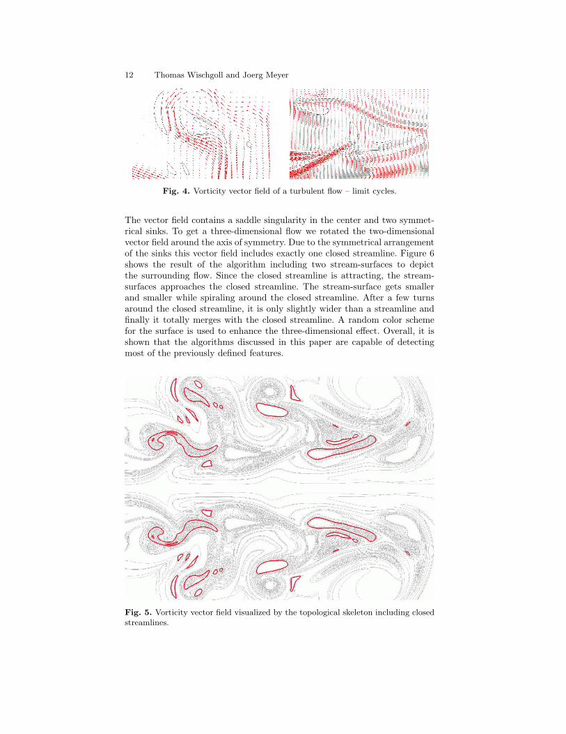
The first example is a simulation of a swirling jet with an inflow into a steadymedium. The simulation originally resulted in a three-dimensional vector fieldbut we used a cutting plane and projected the vectors onto this plane to geta two-dimensional field. In this application one is interested in investigatingthe turbulence of the vector field and in regions where the fluid stays fora very long time. This is necessary because some chemical reactions needa special amount of time. These regions can be located by finding closedstreamlines. Figure 4 shows some of the closed streamlines detected by ouralgorithm in detail. In addition, a hedgehog representation of the vector fieldis given. All these limit cycles are located in the upper region of the vectorfield. Figure 5 shows all closed streamlines of this vector field including thetopological skeleton.

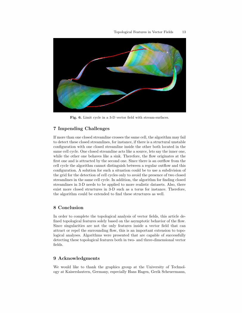
To test our 3-D detection, a synthetically created dataset which includesone closed streamline is used. We first created a two-dimensional vector field.


Fig. 4. Vorticity vector field of a turbulent flow – limit cycles.

The vector field contains a saddle singularity in the center and two symmet-rical sinks. To get a three-dimensional flow we rotated the two-dimensionalvector field around the axis of symmetry. Due to the symmetrical arrangementof the sinks this vector field includes exactly one closed streamline. Figure 6shows the result of the algorithm including two stream-surfaces to depictthe surrounding flow. Since the closed streamline is attracting, the stream-surfaces approaches the closed streamline. The stream-surface gets smallerand smaller while spiraling around the closed streamline. After a few turnsaround the closed streamline, it is only slightly wider than a streamline andfinally it totally merges with the closed streamline. A random color schemefor the surface is used to enhance the three-dimensional effect. Overall, it isshown that the algorithms discussed in this paper are capable of detectingmost of the previously defined features.

Fig. 5. Vorticity vector field visualized by the topological skeleton including closedstreamlines.


Fig. 6. Limit cycle in a 3-D vector field with stream-surfaces.

7 Impending Challenges

If more than one closed streamline crosses the same cell, the algorithm may failto detect these closed streamlines, for instance, if there is a structural unstableconfiguration with one closed streamline inside the other both located in thesame cell cycle. One closed streamline acts like a source, lets say the inner one,while the other one behaves like a sink. Therefore, the flow originates at thefirst one and is attracted by the second one. Since there is an outflow from thecell cycle the algorithm cannot distinguish between a regular outflow and thisconfiguration. A solution for such a situation could be to use a subdivision ofthe grid for the detection of cell cycles only to avoid the presence of two closedstreamlines in the same cell cycle. In addition, the algorithm for finding closedstreamlines in 3-D needs to be applied to more realistic datasets. Also, thereexist more closed structures in 3-D such as a torus for instance. Therefore,the algorithm could be extended to find these structures as well.

8 Conclusion

In order to complete the topological analysis of vector fields, this article de-fined topological features solely based on the asymptotic behavior of the flow.Since singularities are not the only features inside a vector field that canattract or repel the surrounding flow, this is an important extension to topo-logical analyses. Algorithms were presented that are capable of successfullydetecting these topological features both in two- and three-dimensional vectorfields.

9 Acknowledgments

We would like to thank the graphics group at the University of Technol-ogy at Kaiserslautern, Germany, especially Hans Hagen, Gerik Scheuermann,


Xavier Tricoche, and all the students working in this group. Part of this workwas funded by DFG (Deutsche Forschungsgemeinschaft) and Land Rheinland-Pfalz, Germany. Wolfgang Kollmann, Mechanical and Aeronautical Engineer-ing Department of the University of California at Davis, provided us with thevorticity dataset. We are very grateful for this and several helpful hints anddiscussions.

References

1. R. H. Abraham and C. D. Shaw. Dynamics – The Geometry of Behaviour:Bifurcation Behaviour. Aerial Press, Inc., Santa Cruz, 1982.

2. T. J. Aprille and T. N. Trick. A computer algorithm to determine the steady-state response of nonlinear oscillators. IEEE Transactions on Circuit Theory,CT-19(4), July 1972.

3. D. Burkle, M. Dellnitz, O. Junge, M. Rumpf, and M. Spielberg. Visualizingcomplicated dynamics. In A. Varshney, C. M. Wittenbrink, and H. Hagen,editors, IEEE Visualization ’99 Late Breaking Hot Topics, pp. 33 – 36, SanFrancisco, 1999.

4. M. S. Chong, A. E. Perry, and B. J. Cantwell. A General Classification ofThree-Dimensional Flow Fields. Physics of Fluids, A2(5), pp. 765–777, 1990.

5. U. Dallmann. Topological Structures of Three-Dimensional Flow Separations.Technical Report DFVLR-AVA Bericht Nr. 221-82 A 07, Deutsche Forschungs-und Versuchsanstalt fur Luft- und Raumfahrt e.V., April 1983.

6. W. de Leeuw and R. van Liere. Collapsing flow topology using area metrics.In D. Ebert, M. Gross, and B. Hamann, editors, IEEE Visualization ’99, pp.349–354, San Francisco, 1999.

7. M. Dellnitz and O. Junge. On the Approximation of Complicated DynamicalBehavior. SIAM Journal on Numerical Analysis, 36(2), pp. 491 – 515, 1999.

8. G. Fischel, H. Doleisch, L. Mroz, H. Loffelmann, and E. Groller. Case study:visualizing various properties of dynamical systems. In Proceedings of the SixthInternational Workshop on Digital Image Processing and Computer Graphics(SPIE DIP-97), pp. 146–154, Vienna, Austria, October 1997.

9. A. Globus, C. Levit, and T. Lasinski. A Tool for Visualizing the Topology ofThree-Dimensional Vector Fields. In G. M. Nielson and L. Rosenblum, editors,IEEE Visualization ‘91, pp. 33 – 40, San Diego, 1991.

10. E. Groller, H. Loffelmann, and R. Wegenkittl. Visualization of AnalyticallyDefined Dynamical Systems. In Proceedings of Dagstuhl ’97, pp. 71–82. IEEEScientific Visualization, 1997.

11. J. Guckenheimer. Numerical analysis of dynamical systems, 2000.12. J. L. Helman and L. Hesselink. Automated analysis of fluid flow topology.

In Three-Dimensional Visualization and Display Techniques, SPIE ProceedingsVol. 1083, pp. 144–152, 1989.

13. J. L. Helman and L. Hesselink. Visualizing Vector Field Topology in FluidFlows. IEEE Computer Graphics and Applications, 11(3), pp. 36–46, May 1991.

14. D. H. Hepting, G. Derks, D. Edoh, and R. D. Russel. Qualitative analysis ofinvariant tori in a dynamical system. In G. M. Nielson and D. Silver, editors,IEEE Visualization ’95, pp. 342 – 345, Atlanta, GA, 1995.

15. M. W. Hirsch and S. Smale. Differential Equations, Dynamical Systems andLinear Algebra. Academic Press, New York, 1974.

16. J. P. M. Hultquist. Constructing Stream Surface in Steady 3D Vector Fields.In Proceedings IEEE Visualization ’92, pp. 171–177. IEEE Computer SocietyPress, Los Alamitos CA, 1992.


17. A. Inselberg and B. Dimsdale. Parallel Coordinates: a Tool for VisualizingMultidimensional Geometry. In IEEE Visualization ’90 Proceedings, pp. 361–378, Los Alamitos, 1990. IEEE Computer Society.

18. D. N. Kenwright. Automatic Detection of Open and Closed Separation andAttachment Lines. In D. Ebert, H. Rushmeier, and H. Hagen, editors, IEEEVisualization ’98, pp. 151–158, Research Triangle Park, NC, 1998.

19. H. Loffelmann. Visualizing Local Properties and Characteristic Structures ofDynamical Systems. PhD thesis, Technische Universitat Wien, 1998.

20. H. Loffelmann, T. Kucera, and E. Groller. Visualizing Poincare Maps Togetherwith the Underlying Flow. In H.-C. Hege and K. Polthier, editors, MathematicalVisualization, Algorithms, Applications, and Numerics, pp. 315–328. Springer,1997.

21. K. Museth, A. Barr, and M. W. Lo. Semi-Immersive Space Mission Designand Visualization: Case Study of the ”Terrestrial Planet Finder” Mission. InProceedings IEEE Visualization 2001, pp. 501–504. IEEE Computer SocietyPress, Los Alamitos CA, 2001.

22. A. E. Perry and B. D. Fairly. Critical Points in Flow Patterns. Advances inGeophysics, 18B, pp. 299–315, 1974.

23. R. Roussarie. Bifurcations of Planar Vector Fields and Hilbert’s Sixteenth Prob-lem. Birkhauser, Basel, Switzerland, 1998.

24. G. Scheuermann, T. Bobach, H. Hagen, K. Mahrous, B. Hahmann, K. I. Joy,and W. Kollmann. A Tetrahedra-Based Stream Surface Algorithm. In IEEEVisualization ’01 Proceedings, Los Alamitos, 2001. IEEE Computer Society.

25. G. Scheuermann, B. Hamann, K. I. Joy, and W. Kollmann. Visualizing localVetor Field Topology. Journal of Electronic Imaging, 9(4), 2000.

26. X. Tricoche. Vector and Tensor Field Topology Simplification, Tracking andVisualization. PhD thesis, University of Kaiserslautern, 2002.

27. X. Tricoche, G. Scheuermann, and H. Hagen. Topology-Based Visualization ofTime-Dependent 2D Vector Fields. In R. P. D. Ebert, J. M. Favre, editor, Pro-ceedings of the Joint Eurographics–IEEE TCVG Symposium on Visualization,pp. 117–126, Ascona, Switzerland, 2001. Springer.

28. X. Tricoche, T. Wischgoll, G. Scheuermann, and H. Hagen. Topology Trackingfor the Visualization of Time-Dependent Two-Dimensional Flows. Computer &Graphics, pp. 249–257, 2002.

29. M. van Veldhuizen. A New Algorithm for the Numerical Approximation of anInvariant Curve. SIAM Journal on Scientific and Statistical Computing, 8(6),pp. 951 – 962, 1987.

30. R. Wegenkittl, H. Loffelmann, and E. Groller. Visualizing the Behavior of HigherDimensional Dynamical Systems. In R. Yagel and H. Hagen, editors, IEEEVisualization ‘97 Proceedings, pp. 119 – 125, Phoenix, AZ, 1997.

31. T. Wischgoll. Closed Streamlines in Flow Visualization. PhD thesis, UniversitatKaiserslautern, Germany, 2002.

32. T. Wischgoll and G. Scheuermann. Detection and Visualization of ClosedStreamlines in Planar Flows. IEEE Transactions on Visualization and Com-puter Graphics, 7(2), 2001.

33. T. Wischgoll and G. Scheuermann. Locating Closed Streamlines in 3D VectorFields. In Joint Eurographics–IEEE TCVG Symposium on Data Visualization2002, pp. 227–232, Barcelona, Spain, 2002.

34. Y. Yan-qian, C. Sui-lin, C. Lan-sun, H. Ke-cheng, L. Ding-jun, M. Zhi-en, W. Er-nian, W. Ming-shu, and Y. Xin-an. Theory of Limit Cycles. American Mathe-matical Society, Providence - Rhode Island, 1986.

topological features in vector fieldsjmeyer/papers/c-26.pdf · topological features in vector...

Documents