topological data analysis for investigating contagions … · topological data analysis for...

Topological data analysis forinvestigating contagions on networks

Heather A HarringtonResearch Fellow

Mathematical InstituteUniversity of Oxford

HA Harrington (Oxford) TDA for contagions on networks 1 / 18

Collaboration

This work was done in collaboration with

Florian Klimm, University of Oxford, United Kingdom

Miro Kramar, Rutgers University, USA

Konstantin Mischaikow, Rutgers University, USA

Peter J. Mucha, University of North Carolina at Chapel Hill, USA

Mason A. Porter, University of Oxford, United Kingdom

Dane Taylor, University of North Carolina at Chapel Hill, USA

This work is available on arxiv ID 1408.1168.In press, Nature Communications.


Contagion spreading on networks

Social contagion

Information diffusion(innovations, memes, marketing)

Belief and opinion(voting, political views, civil unrest)

Behavior and health

Epidemic contagion

Epidemiology for networks(social networks, technology)

Preventing epidemics(immunization, malware, quarantine)

“Complex contagion”

Adoption of a contagion requiresmultiple contacts with the contagion


Epidemics on networks, then and now

Epidemics historically described bywave front propagation

Motivation

• Epidemics historically described by wave front propagation

Black death-Marvel et al (2014) arXiv 1310.2636

Epidemics: Then and Now

Black death. Marvel et al (2014) arxiv 1310.2636

Modern epidemics driven airline network

Brockman and Helbing (2013) Science


Noisy geometric networks

Consider set V of network nodes with intrinsic locations {w(i)}i∈V in a metricspace (e.g., Earth’s surface).

Restrict to nodes that lie on a manifold M that is embedded in an ambientspace A (i.e., w(i) ∈M ⊂ A).

“Node-to-node distance” refers to the distance between nodes in thisembedding space A (here we use the Euclidean norm ‖ · ‖2).

Place nodes in underlying manifold and add two types oftwo edge types:

Geometric edges added between nearby nodes

Non-geometric edges added uniformly at random

Origins

Inherent heterogeneity in spatial networks

Noise in networks/ noise in data

(a) (b) (c)


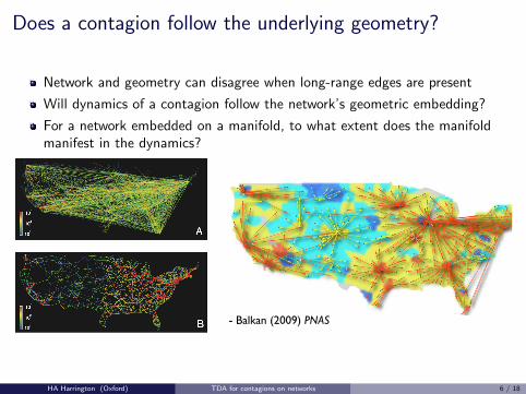
Does a contagion follow the underlying geometry?

Network and geometry can disagree when long-range edges are present

Will dynamics of a contagion follow the network’s geometric embedding?

For a network embedded on a manifold, to what extent does the manifoldmanifest in the dynamics?

Network vs Geometry• Network and geometry can significantly disagree when long-range

edges are present.

• Will dynamics follow the geometry or network?

Motivation

- Balkan (2009) PNAS


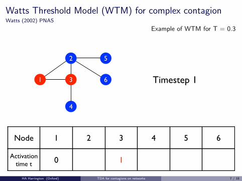
Watts Threshold Model (WTM) for complex contagionWatts (2002) PNAS

For time t = 1, 2, . . . binary dynamics at each node n ∈ Vxn(t) = 1 contagion adopted by time t

xn(t) = 0 contagion not adopted by time t

Node n adopts the contagion if the fraction fn(t) of its neighbors that haveadopted the contagion surpasses a threshold T .

xn(t + 1) = 1 if xn(t) = 0 and fn(t) > T

Otherwise xn(t + 1) = xn(t), i.e., no change

Note: the number of adopters in this model is non-decreasing.



Example of WTM for T = 0.3An example with T=0.3

1

2

3 6

5

4

Timestep 0

Node 1 2 3 4 5 6

Activation time t 0

Contagion dynamics for topological data analysisHA Harrington (Oxford) TDA for contagions on networks 7 / 18



1

2

3 6

5

4

Timestep 1

Node 1 2 3 4 5 6

Activation time t 0 1




1

2

3 6

5

4

Timestep 2

Node 1 2 3 4 5 6

Activation time t 0 2 1 2




1

2

3 6

5

4

Timestep 3

Node 1 2 3 4 5 6

Activation time t 0 2 1 2 3 3


Contagion phenomena

Spreading of contagion phenomena can be described by edge types:

Wave front propagation (WFP) by spreading across geometric edges

Appearance of new clusters (ANC) of contagion from spreading acrossnon-geometric edges

0

5

0

50

geometric edgenon-geometric edge

cluster appearance for small T

wavefront propagation for moderate T

contagion seed new contagion clustercluster containing

contagion seed

activ

ation

tim

e

activ

ation

tim

e


WFP and APC depend on threshold T

Activation time is the time at which the node adopts the contagion

for adopting the social “contagion,” for which we assume Ti = Tfor simplicity. Focusing on two phenomena, wavefront propagation(WFP) along the underlying geometric network and the appearanceof new contagion clusters (ANC), we find diverse regimes of dynam-ics. These are studied on both empirical and synthetic networks. Togain insight, we present a bifurcation analysis for a class of noisygeometric networks we refer to as noisy ring lattices, for which weanalyze the presence versus absence of WFP and ANC and their re-spective rates (i.e., the speed of WFP and the occurrence frequencyof ANC). In Fig. 1 we illustrate WFP and ANC and discuss theirdependence on the contagion parameter T .

0

5

0

50

geometric edge

non-geometric edge

cluster appearance for small T

wavefront propagation for moderate T

contagion seed new contagion cluster

cluster containingcontagion seed

activa

tion

tim

e

activa

tion

tim

e

Fig. 1. (top panel) Watts threshold model (WTM) [54] with uniform threshold Ton a noisy geometric network containing geometric edges along a manifold (in this

case, a 2D lattice) and non-geometric edges introducing shortcuts in the network.

We study two phenomena regarding the evolution of contagion clusters (see shaded

areas): Wavefront propagation (WFP) describes the outward expansion of a conta-

gion cluster’s boundary. The appearance of a new contagion cluster (ANC) occurs

when the contagion spreads exclusively across non-geometric edges (see dashed ar-

row). (lower panels) WFP and ANC may be observed through the activation times of

the nodes (the time at which a given node adopts the contagion), which are depen-

dent on T . For small T , frequent ANC leads to rapid dissemination. For moderate

T , little to no ANC occurs and WFP leads to slow dissemination. For large T , there

is no spreading (not shown). For a given network, activation times collected across

N realizations of contagion (with varying initial conditions) map the network nodes

to a point cloud in RN , which we refer to as a WTM map. We study the extent to

which the dynamics follows the network’s embedding in the metric space by analyzing

the geometry, dimensionality and topology of the WTM map.

We additionally address an important but poorly-understoodquestion: To what extent do the spreading dynamics follow the man-ifold on which the network is embedded? To this end, we introducea mapping of network nodes as a point cloud based on WTM con-tagions. By analogy to diffusion maps [13] and similar ideas in di-mension reduction [3, 15, 53], we use the term WTM maps for thesemaps. We examine the geometry, topology, and dimensionality ofWTM maps and compare them to those of the underlying manifoldof the noisy geometric network on which the dynamics occur. Thisapproach aligns our work with the fields of manifold learning anddimension reduction [3,13,15,20,52,53], which focus on data analy-sis and complement our dynamical-systems approach. Additionally,because WTM maps are based on non-conservative dynamics (e.g.,for the WTM the number of nodes that have adopted the contagionis non-decreasing as nodes cannot un-adopt the contagion) [21], theyprovide a contrast to techniques that are based on conservative dy-namics like ordinary random walks and diffusion. Thus the motiva-tion for this work is twofold: (i) introduce a methodology for study-ing the extent to which contagion follows the underlying structure ofa noisy geometric network, and (ii) introduce a methodology for in-ferring low-dimensional (e.g., manifold) structure in networks basedon WTM contagions.

ModelNoisy Geometric Networks. As we mentioned previously, noisygeometric networks are a class of networks that arise from geometricnetworks [2] but also include non-geometric, “noisy” edges. Specifi-cally, consider network nodes V with intrinsic locations {z(i)}i2V ina metric space. We will restrict our attention in the present paper tonodes that lie on a manifold M that is embedded in some (possiblyhigher-dimensional) ambient metric space A (i.e., z(i) 2 M ⇢ A).We use the term “node-to-node distance” to refer to the distance be-tween nodes in this embedding space A, which we equip with theEuclidean norm k · k2 (although other metrics could be used [4]).To form a synthetic noisy geometric network, we construct such anodal embedding and add two families of edges: a set of geometricedges E(G), such that (i, j) 2 E(G) if and only if nodes i and j aresufficiently close to one another on the manifold M; and a set of non-geometric edges E(NG), which are selected using some random pro-cess for pairs of nodes (i, j) such that (i, j) 62 E(NG) and i 6= j. InFigs. 2(a) and 2(b) we show examples of such a construction, wherenon-geometric edges are added uniformly at random. In Fig. 2(c) weshow an alternative construction motivated by applications in dimen-sion reduction [3, 13, 20, 53] and left for further research.

(a) (b) (c)

Fig. 2. Noisy geometric networks in which geometric edges (blue) connect nodes

that are nearby on the manifold and non-geometric edges (red) connect distant

nodes, which are shown for three manifolds: (a) circle embedded in R2; (b) spherical

surface (2D) in R3; and (c) bounded plane (2D) embedded (nonlinearly) in R3 in

a configuration known as the “swiss roll” [53]. In panels (a) and (b) non-geometric

edges are added uniformly at random. In panel (c) noise is added to the nodes’ lo-

cations in the ambient space and edges are formed between nodes that are nearby in

the ambient space. In this case, edges between nodes that are nearby with respect to

the ambient space but not the manifold, are interpreted as non-geometric edges.

As an illustrative example, consider the noisy ring lattice inFig. 2(a), which is similar to the Newman-Watts variant of the Watts-Strogatz small-world model [38,41,55]. Specifically, we consider Nnodes that are uniformly spaced along the unit circle in R2. Geo-metric edges are then added so that every node i is connected to itsd(G) nearest neighbor nodes (with no self edges). We then add d(NG)

non-geometric edges to each node, connecting the ends of edges uni-formly at random while avoiding self-edges and multi-edges. Theresulting network is a (d(G) + d(NG))-regular network containingNd(G)/2 geometric edges and Nd(NG)/2 non-geometric edges andis thus specified by three parameters: N , d(G) and d(NG). Note thatthis construction assumes N and d(G) are even. Fig. 2(a) shows sucha network with N = 20 and (d(G), d(NG)) = (4, 2). In Sec. 4of the SI appendix we present additional models of noisy geometricnetworks on a ring manifold.

Watts threshold model (WTM). Following Ref. [54], we defineWTM contagion as follows: Given a network with a set of nodesV and a set of edges E given by an adjacency matrix A, we de-note by xi(t) the state of node i 2 V at time t, where xi(t) = 1[xi(t) = 0] indicates adoption [non-adoption]. We initialize a con-tagion at time t = 0 by choosing a set of nodes S ⇢ V and set-ting xi(0) = 1 for i 2 S and xi(0) = 0 for all other nodes. Werefer to S as the “contagion seed.” We consider synchronous up-dating in discrete time [46], such that a node i that has not alreadyadopted the contagion at time t [i.e., xi(t) = 0] will adopt it upon

2 www.pnas.org/cgi/doi/10.1073/pnas.0709640104 Footline Author


Noisy ring latticeAim I: Analyze the Watts threshold model (WTM) on noisy geometric network

Simple network model

Ambient space: A = R2

Ring manifold: M = (x , y) ∈ R2 s.t. x2 + y2 = 1

Uniformly sampled a ring manifold

Network is given by 3 parameters:

1 Number of nodes N

2 Geometric degree dG

3 Non-geometric degree dNG

4 Ratio of non-geometric to geometric edges,α = dNG/dG

(a) (b) (c)

In this example, N = 20, dG = 4, dNG = 2, α = 1/2


Critical thresholds for noisy ring latticeTo what extent do the dynamics of a contagion spreads by WFP versus ANC?

Wavefront propagation (WFP) is governed by the critical thresholds:

T(WFP)k =

d (G)/2− k

d (G) + d (NG), k = 0, 1 . . . , d (G)/2. (1)

Note: for T ≥ T(WFP)0 , there is no WFP.

Appearance of new clusters (APC) has a sequence of critical thresholds:

T(ANC)k =

d (NG) − k

d (G) + d (NG), k = 0, 1 . . . , d (NG). (2)


Bifurcation diagram and trait regimes

Consider the case when k = 0

similar to the analysis above we find a sequence of critical thresholds,

T(ANC)k =

d(NG) � k

d(G) + d(NG), k = 0, 1 . . . , d(NG). [2]

It follows that for T(ANC)k+1 T < T

(ANC)k , ANC phenomena will

be similar, and will depend on the probability that a node will havek non-geometric neighbors that have adopted the contagion at time t,which is proportional to [q(t)/N ]k (see Sec. 1 of the SI Appendix).

0 0.5 10

0.2

0.4

0.6

! = d (NG)/d (G)

thre

shold

(T)

Bifurcat ion Diagram

0 0.5 10

0.2

0.4

0.6

! = d (NG)/d (G)th

resh

old

(T)

WFP and ANC traits

no WFPno ANC

WFPANC

(b)(a)

IV

I I I

I I

I

WFPno ANC

no WFPANC

slowWFP

l ike lyANC

unl i ke lyANC

fastWFP I

II

III

IV

10 20 30 40 500

50

100

150

200

t ime (t )

q(t)

C ontagion Growth

10 20 30 40 500

5

10

15

t ime (t )

C(t)

Number of C lusters

T=0.05

T=0.2

T=0.3

T=0.45

(d)(c)

dqdt

= 2 dG

2 t

dqdt

= 2t

(a)

(c) (d)

(b)

slWF

fastWF

IIIIII

e le l yANC

l ike lylylyANC

fastWFPP I

IIII

no WFPno ANC

WFPno ANC

no WFPANC

WFPANC

unlikelyANC

likelyANC

fastWFP

slowWFP

!!

Fig. 4. (a) Critical thresholds T(WFP)0 (solid line) and T

(ANC)0 (dashed line)

given by Eqs. [ 1 ] and [ 2 ] are shown versus the ratio of non-geometric to geomet-

ric edges ↵ = d(NG)/d(G). These indicate four qualitatively di↵erent contagion

regimes characterized by the presence versus absence of WFP and ANC. (b) Eqs. [ 1 ]and [ 2 ] for additional k further describe WFP and ANC and are shown for dG = 6(lines descend with k). Fixing (d(G), d(NG)) = (6, 2) (i.e., ↵ = 1/3), we

find four contagion regimes (denoted I-IV), where increasing T corresponds to slower

WFP and less frequent ANC. In particular, for (d(G), d(NG)) = (6, 2) (i.e.,

↵ = 1/3), we find four regimes of similar WFP and ANC traits (see labels I-IV),

which are illustrated in the lower panels. (c) For T 2 {0.05, 0.2, 0.3, 0.45}, we

plot the contagion size q(t) versus time t for one realization of contagion with cluster

seeding [i.e., q(0) = 1 + d(G) + d(NG) = 9]. We observe, as expected, that

the growth rate decreases with T . In particular, for regime III (e.g., T = 0.3),

the contagion spreads strictly via WFP, which initially spreads at a rate of one node

per time step (both clockwise and counterclockwise along the ring), but eventually

accelerates to d(G)/2 nodes per time step. (d) We plot the number of contagion

clusters C(t) versus t. As expected, C(t) only increases above its initial value of

C(0) = 1 + d(NG) = 3 for regimes I and II (for which T < T(ANC)0 ). There

is no spreading for regime IV.

In Fig. 4(a), we show a bifurcation diagram summarizing theWTM dynamics for variable contagion threshold T and ratio of non-geometric edges to geometric edges, ↵ = dNG/dG. The solidand dashed curves, respectively, describe Eq. [1] and Eq. [2]for k = 0. These correspond to T

(WFP)0 = 1/(2 + 2↵) and

T(ANC)0 = ↵/(↵ + 1), which intersect at (↵, T ) = (1/2, 1/3)

and yield four regimes of contagion dynamics characterized by thepresence versus absence of WFP and ANC. In Fig. 4(b), we plotEq. [1] and Eq. [2] with other k values for d(G) = 6 (descend-ing lines correspond to increasing k). Observe that increasing T forfixed ↵ leads to slower WFP and less frequent ANC. In particular,

for (d(G), d(NG)) = (6, 2) (i.e., ↵ = 1/3), we find four regimes ofsimilar WFP and ANC traits (see labels I-IV).

In Figs. 4(c) and 4(d) we illustrate dynamics from these forregimes by choosing T 2 {0.05, 0.2, 0.3, 0.45} and plotting the sizeq(t) of the contagion [Fig. 4(c)] and the number of contagion clustersC(t) [Fig. 4(d)] versus time t. These results confirm our analysis:For T = 0.05, the contagion saturates the network [i.e., q(t) ! N ]very rapidly due in part to the appearance of many contagion clustersearly in the contagion process. For T = 0.2, the contagion satu-rates the network relatively rapidly due to the appearance of somenew contagion clusters. For T = 0.3, the contagion saturates thenetwork slowly, as no new contagion clusters appear and the conta-gion spreads only via WFP. For T = 0.45, the contagion does notsaturates the network, as neither WFP nor ANC occur.

Comparing WTM maps to the network’s underlying mani-fold. In this section we analyze WTM-maps for noisy ring lattices inseveral ways: geometrically, topologically, and in terms of dimen-sionality. Such point cloud analytics identify parameter regimes inwhich characteristics of the manifold appear also in the WTM maps,offing a methodology to asses the extent to which the contagion ad-heres to the network’s underlying manifold. These results are foundto be in good agreement with our theory given by Eqs. [1] and [2].

In Fig. 5 we study WTM maps for a noisy ring lattice withN = 200 and (d(G), d(NG)) = (6, 2). In Fig. 5(a), we illustrateWTM maps for four threshold values T 2 {0.05, 0.2, 0.3, 0.45},which correspond to the four regimes of contagion dynamics pre-dicted by Eqs. [1] and [2] [see labels I-IV in Fig. 4(b)]. To visualizethe N -dimensional WTM maps, we use principle component analy-sis to project onto R2 [14, 52, 53]. The color of each point reflectsthe activation time for the corresponding node for one realizationof the WTM contagion, which is shown below each point cloud inpanel (b). In particular, in panels (a) and (b) dark blue nodes denotethe contagion seed (i.e., under cluster seeding). Nodes colored graynever adopt the contagion (i.e., they have an infinite activation time),which for practical purposes (e.g., visualization) we set the activationtime for such nodes to be 2N rather than 1. Note that for regime III,the point cloud appears to best resemble (up to rotation) the nodes’intrinsic locations {z(i)} along the ring manifold M ⇢ R2 (i.e., theunit circle), which is expected as this regime corresponds to WFP andno ANC (i.e., the contagion follows the manifold).

In Fig. 5(c), we summarize characteristics of WTM maps fordifferent thresholds T . For each given T 2 [0, 0.6], we analyze thepoint cloud’s geometry (top), dimensionality (center), and topology(bottom). Specifically, the geometry of the point cloud {y(i)} is com-pared to that for the node locations {z(i)} on the manifold by comput-ing the Pearson correlation coefficient comparing the node-to-nodedistances for the two point clouds, i.e., comparing ||y(i)�y(j)||2 and||z(i) � z(j)||2 for all i, j 2 V . The dimensionality is studied by ex-amining the residual variance [14, 53] of the point cloud {y(i)}, andcomputing the smallest dimension such that less than 5% of the vari-ance is lost when projecting to a lower dimension using PCA [14,53].We refer to this dimension as the “embedding dimension” P . Fi-nally, the topology is studied by examining the persistence diagramof a Vietoris-Rips filtration generated by the point cloud [17, 29]. Inparticular, we define � = l1 � l2 where l1 and l2 are life spans ofthe most dominant and second most dominant topological feature inthe Vietoris-Rips filtration. Large � indicates the presence of a sin-gle dominant 1-cycle (i.e., ring) in the point cloud. As expected byour analysis, for the regime exhibiting WFP and no ANC, regime III,characteristics of the manifold M are identified in point clouds re-sulting from WTM maps for this regime. Namely, for this regime thepoint cloud has similar geometry (i.e., indicated by large ⇢), topology(i.e., indicated by large �), and embedding dimension (i.e., indicatedby P = 2) as the manifold M. See the Methods and Materials sec-


T(WFP)0 =

1

(2 + 2α)

−−−− T(ANC)0 =

α

(α + 1)

Lines intersect at (α,T ) = (1/2, 1/3)

Four regimes of contagion dynamics characterized by the presence versus absenceof WFP and ANC.


Bifurcation diagram and trait regimes

Consider increasing values of k (decreasing lines) for fixed dG = 6

similar to the analysis above we find a sequence of critical thresholds,

T(ANC)k =

d(NG) − k

d(G) + d(NG), k = 0, 1 . . . , d(NG). [2]

It follows that for T(ANC)k+1 ≤ T < T

(ANC)k , ANC phenomena will

be similar, and will depend on the probability that a node will havek non-geometric neighbors that have adopted the contagion at time t,which is proportional to [q(t)/N ]k (see Sec. 1 of the SI Appendix).

0 0.5 10

0.2

0.4

0.6

α = d (NG)/d (G)

thre

shold

(T)

Bifurcat ion Diagram

0 0.5 10

0.2

0.4

0.6

α = d (NG)/d (G)

thre

shold

(T)

WFP and ANC traits

no WFPno ANC

WFPANC

(b)(a)

IV

I I I

I I

I

WFPno ANC

no WFPANC

slowWFP

l ike lyANC

unl i ke lyANC

fastWFP I

II

III

IV

10 20 30 40 500

50

100

150

200

t ime (t )

q(t)

C ontagion Growth

10 20 30 40 500

5

10

15

t ime (t )

C(t)

Number of C lusters

T=0.05

T=0.2

T=0.3

T=0.45

(d)(c)

dq

dt= 2 dG

2 t

dq

dt= 2t

(a)

(c) (d)

(b)

slWF

fastWF

IIIIII

e le l yANC

l ike lylylyANC

fastWFPP I

IIII

no WFPno ANC

WFPno ANC

no WFPANC

WFPANC

unlikelyANC

likelyANC

fastWFP

slowWFP

αα

Fig. 4. (a) Critical thresholds T(WFP)0 (solid line) and T

(ANC)0 (dashed line)

given by Eqs. [ 1 ] and [ 2 ] are shown versus the ratio of non-geometric to geomet-

ric edges α = d(NG)/d(G). These indicate four qualitatively different contagion

regimes characterized by the presence versus absence of WFP and ANC. (b) Eqs. [ 1 ]and [ 2 ] for additional k further describe WFP and ANC and are shown for dG = 6(lines descend with k). Fixing (d(G), d(NG)) = (6, 2) (i.e., α = 1/3), we

find four contagion regimes (denoted I-IV), where increasing T corresponds to slower

WFP and less frequent ANC. In particular, for (d(G), d(NG)) = (6, 2) (i.e.,

α = 1/3), we find four regimes of similar WFP and ANC traits (see labels I-IV),

which are illustrated in the lower panels. (c) For T ∈ {0.05, 0.2, 0.3, 0.45}, we

plot the contagion size q(t) versus time t for one realization of contagion with cluster

seeding [i.e., q(0) = 1 + d(G) + d(NG) = 9]. We observe, as expected, that

the growth rate decreases with T . In particular, for regime III (e.g., T = 0.3),

the contagion spreads strictly via WFP, which initially spreads at a rate of one node

per time step (both clockwise and counterclockwise along the ring), but eventually

accelerates to d(G)/2 nodes per time step. (d) We plot the number of contagion

clusters C(t) versus t. As expected, C(t) only increases above its initial value of

C(0) = 1 + d(NG) = 3 for regimes I and II (for which T < T(ANC)0 ). There

is no spreading for regime IV.

In Fig. 4(a), we show a bifurcation diagram summarizing theWTM dynamics for variable contagion threshold T and ratio of non-geometric edges to geometric edges, α = dNG/dG. The solidand dashed curves, respectively, describe Eq. [1] and Eq. [2]for k = 0. These correspond to T

(WFP)0 = 1/(2 + 2α) and

T(ANC)0 = α/(α + 1), which intersect at (α, T ) = (1/2, 1/3)

and yield four regimes of contagion dynamics characterized by thepresence versus absence of WFP and ANC. In Fig. 4(b), we plotEq. [1] and Eq. [2] with other k values for d(G) = 6 (descend-ing lines correspond to increasing k). Observe that increasing T forfixed α leads to slower WFP and less frequent ANC. In particular,

for (d(G), d(NG)) = (6, 2) (i.e., α = 1/3), we find four regimes ofsimilar WFP and ANC traits (see labels I-IV).

In Figs. 4(c) and 4(d) we illustrate dynamics from these forregimes by choosing T ∈ {0.05, 0.2, 0.3, 0.45} and plotting the sizeq(t) of the contagion [Fig. 4(c)] and the number of contagion clustersC(t) [Fig. 4(d)] versus time t. These results confirm our analysis:For T = 0.05, the contagion saturates the network [i.e., q(t) → N ]very rapidly due in part to the appearance of many contagion clustersearly in the contagion process. For T = 0.2, the contagion satu-rates the network relatively rapidly due to the appearance of somenew contagion clusters. For T = 0.3, the contagion saturates thenetwork slowly, as no new contagion clusters appear and the conta-gion spreads only via WFP. For T = 0.45, the contagion does notsaturates the network, as neither WFP nor ANC occur.

Comparing WTM maps to the network’s underlying mani-fold. In this section we analyze WTM-maps for noisy ring lattices inseveral ways: geometrically, topologically, and in terms of dimen-sionality. Such point cloud analytics identify parameter regimes inwhich characteristics of the manifold appear also in the WTM maps,offing a methodology to asses the extent to which the contagion ad-heres to the network’s underlying manifold. These results are foundto be in good agreement with our theory given by Eqs. [1] and [2].

In Fig. 5 we study WTM maps for a noisy ring lattice withN = 200 and (d(G), d(NG)) = (6, 2). In Fig. 5(a), we illustrateWTM maps for four threshold values T ∈ {0.05, 0.2, 0.3, 0.45},which correspond to the four regimes of contagion dynamics pre-dicted by Eqs. [1] and [2] [see labels I-IV in Fig. 4(b)]. To visualizethe N -dimensional WTM maps, we use principle component analy-sis to project onto R2 [14, 52, 53]. The color of each point reflectsthe activation time for the corresponding node for one realizationof the WTM contagion, which is shown below each point cloud inpanel (b). In particular, in panels (a) and (b) dark blue nodes denotethe contagion seed (i.e., under cluster seeding). Nodes colored graynever adopt the contagion (i.e., they have an infinite activation time),which for practical purposes (e.g., visualization) we set the activationtime for such nodes to be 2N rather than ∞. Note that for regime III,the point cloud appears to best resemble (up to rotation) the nodes’intrinsic locations {z(i)} along the ring manifold M ⊂ R2 (i.e., theunit circle), which is expected as this regime corresponds to WFP andno ANC (i.e., the contagion follows the manifold).

In Fig. 5(c), we summarize characteristics of WTM maps fordifferent thresholds T . For each given T ∈ [0, 0.6], we analyze thepoint cloud’s geometry (top), dimensionality (center), and topology(bottom). Specifically, the geometry of the point cloud {y(i)} is com-pared to that for the node locations {z(i)} on the manifold by comput-ing the Pearson correlation coefficient comparing the node-to-nodedistances for the two point clouds, i.e., comparing ||y(i)−y(j)||2 and||z(i) − z(j)||2 for all i, j ∈ V . The dimensionality is studied by ex-amining the residual variance [14, 53] of the point cloud {y(i)}, andcomputing the smallest dimension such that less than 5% of the vari-ance is lost when projecting to a lower dimension using PCA [14,53].We refer to this dimension as the “embedding dimension” P . Fi-nally, the topology is studied by examining the persistence diagramof a Vietoris-Rips filtration generated by the point cloud [17, 29]. Inparticular, we define ∆ = l1 − l2 where l1 and l2 are life spans ofthe most dominant and second most dominant topological feature inthe Vietoris-Rips filtration. Large ∆ indicates the presence of a sin-gle dominant 1-cycle (i.e., ring) in the point cloud. As expected byour analysis, for the regime exhibiting WFP and no ANC, regime III,characteristics of the manifold M are identified in point clouds re-sulting from WTM maps for this regime. Namely, for this regime thepoint cloud has similar geometry (i.e., indicated by large ρ), topology(i.e., indicated by large ∆), and embedding dimension (i.e., indicatedby P = 2) as the manifold M. See the Methods and Materials sec-


=0.45

=0.3

=0.2

=.05

incr

easi

ng k

Four regimesI : T ∈ (0; .125), II : T ∈ (.125; .25), III : T ∈ (.25; .375), IV : T > .375


WTM maps: contagion maps based on WTM contagionsAim II: To what extent do the spreading dynamics follow the manifold on which the network isembedded? To study this we construct and analyze WTM maps!

A WTM map is a nonlinear map of nodes to a high-dimensional point cloud in ametric space based on the activation times from N realisations of WTMcontagions.

Initialise the j-th contagion centred at node j = 1, . . .N.

Record activation time x(i)j for each node i and contagion j .

Each node i maps to the point x(i) = [x(i)1 , x

(i)2 , . . . , x

(i)N ]

V 7→ {x(i)}i∈V ∈ RN

The WTM map V 7→ {x(i)}i∈V ∈ RN yields a high dimensional point cloud.


WTM maps: contagion maps based on WTM contagionsAim II: To what extent do the spreading dynamics follow the manifold on which the network isembedded? To study this we construct and analyze WTM maps!

Visualise N dimensional WTM map after 2D mapping via PCA.WTM maps

for each node activation time under each possible contagion with different seed node

NxN non-symmetric matrix

contagion seed

activ

atio

n tim

e

25

50

ring structure already observable

Contagion dynamics for topological data analysis

Observe ring structure already. For each node, have activation time under eachpossible contagion with different seed node. N × N non-symmetric matrix.


Analysis using geometry, topology and dimensionalityHow does the distance between two nodes in a point cloud from a WTM map relate to thedistance between those nodes in the original metric-space?

Geometry of the the node-to-node distances for the two point clouds (WTMmap and underlying manifold) is compared by computing Pearson correlationcoefficient ρ.

Persistence of 1-cycles (∆ describes lifespan of cycles) using persistenthomology

(a) (b) (c) (d)

Figure 1: (a) A Point cloud X given by a noisy sample of a circle. (b-d) Sets Xr for r = 0.22, 0.6, 0.85.Homology of Xr can be approximated by a Vietoris-Rips complex given by the vertices, edges and trianglesshown in the the panels. The first loop in Xr is created at r = 0.22. This loop is due to the noisy samplingand is filled in almost immediately. The dominant loop show in (c) is formed at r = 0.5 and persists untilr = 0.81.

Given two distances m and m(WTM) for each pair of nodes (i, j), we compute the Pearson correlationcoefficient ⇢ between them over all unordered pairs. Because i 6= j for distinct nodes, there are N(N �1)/2such pairs.

Note that such a calculation requires the activation time y(i)j to be finite for all nodes i and realizations

of contagion, j. This, however, is not the case whenever there is a node that never becomes activated.For example, y

(i)j = 1 for all nodes other than the seed if the threshold T is sufficiently large to prevent

spreading (i.e., T � max{T(WFP)0 , T

(ANC)0 } for the case of the noisy ring lattice). For practical purposes,

we use y(i)j = 2N in such cases, where we note that y

(i)j N � 1 for any numerical simulation in which

node i eventually becomes infected.

3.2 Topological Analysis

In this section we explain how to analyze topology of a point cloud X = {x1, x2, . . . , xn} 2 RN obtainedusing the WTM map. The set X has a very simple topology. If xi 6= xj for i 6= j, then X consist of ndistinct connected components corresponding to the points xi. There are no loops present in the data setX . To infer the topology of the underlaying manifold form which the data cloud was sampled we study thetopology on different spacial scales. In particular we are interested in the topology of the sets

Xr =[

1in

{x 2 RN : kxi � xk r},

for different values of r 2 [0,1).Fig. 1 shows a data set X sampled from a noisy ring. For r = 0 there are 10 distinct connected

components corresponding to the points. As we increase r four of the components merge together andcreate a loop shown in Fig 1(b). This loop is filed in very soon after it was created. After this loop is filedin, another loop appears. This loop is present for wider range of r and seems to be more relevant than thefirst loop. To make this statement more quantitative we will employ persistent homology [69, 70].

To every set Xr one can assign homology groups Hn(Xr) where n 2 Z. Rank of the group Hn(Xr)denoted by �n is the number of n dimensional topological features present in Xr. In particular, �0 countsthe number of connected components, �1 the number of loops and �2 represents the cavities. Fact that

8

Figure 2: �1 persistence diagram for the filtration Xr. It contains a single dominant point corresponding tothe prominent loop along which the points in X are arranged.

Xr ✓ Xr0 for r r0 is very important. A collection of sets with this property is called a filtration. For afiltration Xr we can identity the topological features of Xr at different values of r.

In this paper we are interested in understanding the loops of Xr as we vary the value of r. This infor-mation is encoded by the �1 persistence diagram. Fig. 2 shows the �1 persistence diagram for the aboveexample. There are two points in this diagram corresponding to two distinct loops present in Xr. The birthaxis of the point is the value of r at which the loop corresponding to this point appeared in Xr. The deathcoordinate indicates when the loop is filled in. For every point (rb, rd) in the persistence diagram we defineits life span as rd � rb. Topological feature with longer life span are more dominant. In our example there isone point with a short life span corresponding to a small loop present due to the noisy sampling. The otherpoint with much larger life span corresponds to the ring structure of the sampled manifold. In general the�1 persistence diagram is a multi set containing one point for every loop.

Computing the persistence homology of Xr is complicated. The nerve theorem [68] guarantees that thehomology of Xr is equal to the homology of a corresponding Cech complex. However constructing a Cechcomplex is still computationally expensive. Therefore we use its approximation known as Vietoris-Ripscomplex. For a given data set X = {x1, x2, . . . , xn} 2 RN and r 2 R the Vietoris-Rips complex V Rr

is a complex consisting of the simplices (xs1 , xs2 , . . . , xsk) such that kxsi � xsjk2 r for all si and sj .

Computation of persistent homology from a point cloud is numerically demanding task, and the requiredmemory resources expand rapidly as one considers higher-dimensional objects. We are only interestedin identifying the loops in V Rr so it is enough for us to use only 0-simplices (points), 1-simplices (linesegments), and 2-simplices (triangles).

To compute the persistent homology we used the software package Perseus [65, 67] (version 3.0 Beta)and double-checked some of the results using the javaPlex Persistent Homology Library [66]. Perseus isequipped to handle a diverse variety of input complexes—including simplicial complexes, and Vietroris-Rips complexes. Construction of the Vietroris-Rips filtration only requires distances of the data points.We define the distance between nodes i and j by m(WTM)(i, j) and use a distance matrix Y , with entries[Y ]ij = d(WTM)(i, j), to build the Vietoris-Rips filtration V Rr.

As mentioned above, we are interested in analyzing the loops in the point cloud generated by the WTMmaps. Therefore we analyze the �1 persistence diagrams for several values of the WTM threshold T 2[0, 0.5] and several choices for non-geometric degrees d(NG) 2 [0, 20]. We consider networks with N = 100

9

Embedding dimension P is computed by studying p-dimensional projectionsof the WTM map obtained via principle component analysis (such that theresidual variance Rp for the projection onto Rp < 0.05).


Analysis using topology: persistent homologyWe are interested in persistence of 1-cycles

Analyze the point could by constructing a Vietoris-Rips filtration and calculate itspersistent homology.

!

l 1de

ath

l 2

!

0.8

0.6

0.4

0.2

0

birth0.8 1

1

0.60.40.20

1

(r (i

))

(r (i ))b

d

persistence diagramWe define the

the ring stability:

� = l1 � l2

longest circle

2nd longest circle


Persistence Homology

`i = rd(i)− rb(i)We define the ring stability ∆ = `1 − `2.


Analysis using topology: persistent homologyWe are interested in persistence of 1-cycles

(a)

(b) seed node

755025

activation time

never activated

0

0.5

1

threshold T

!

0

10

20

threshold T

P

0 0.3 0.60

30

60

threshold (T )

"

(c)I III IVII I III IVII

Fig. 5. (a) Point clouds resulting from WTM maps that are constructed with (I) T = 0.05, (II) T = 0.2, (III) T = 0.3, and (IV) T = 0.45 for the noisy ring lattice

shown in panel (b) (which has N = 200 nodes, each with d(G) = 6 geometric and d(NG) = 2 non-geometric edges). The color of each node, or corresponding point,

denotes its activation time for one realization of contagion. Nodes in the contagion seed are dark blue and nodes that never adopt the contagion are gray. For visualization

purposes, we show the two-dimensional projections of the N -dimensional point clouds after applying principle component analysis [14, 52]. (c) We analyze point clouds

resulting from WTM maps with variable threshold T with respect to three criteria: geometry (top), dimensionality (center), and topology (bottom). We study the geometry

by considering node-to-node distances (in the metric of the embedding space, which in this case is the Euclidean norm) and computing the Pearson correlation coe�cient ⇢

between these distances for the WTM map, {yi} 2 RN , and the original node locations, {z(i)} 2 R2. We examine the dimensionality through its embedding dimension

P , which is calculated by studying the residual variance [14, 53]. We examine the topology by studying the persistent homology when applying a Vietoris-Rips filtration to

the point cloud [17, 29], where � denotes the di↵erence in lifespans for the two most persistent 1-cycles. Vertical dashed lines denote predicted shifts in contagion dynamics

given by Eqs. [ 1 ] and [ 2 ] [see Fig. 4(b)]. Note that there are infinite activation times and the WTM map is not well defined for T � T(WFP)0 = 3/8 (shaded region).

As expected for regime III, the geometry, topology, and dimensionality of the point cloud recovers that of the manifold M, as indicated by large correlation ⇢ ⇡ 1, an

estimated embedding dimension P = 2, and a single dominant 1-cycle (i.e., a ring) as indicated by large �. See the Methods section and the SI for further discussion of

these point-cloud analytics.

tion and the Sec. 3 of the SI Appendix for additional discussion ofthese point cloud analytics.

In Fig. 6, we analyze WTM maps with variable T appliedto noisy ring lattices with variable ↵ = d(NG)/d(G) (shown forN = 200, d(G) = 20 and variable d(NG)). For each point cloudwe study (a) geometry through ⇢, (b) dimensionality through P , and(c) topology through �. Transitions between the qualitatively dif-ferent regimes of these properties closely resemble the bifurcationstructure given Eqs. [1] and [2] with k = 0, which are shown by thesolid and dashed curves, respectively. In particular, for the regimeexhibiting WFP and no ANC, the geometry, embedding dimensionand topology of the underlying manifold giving rise to the noisy ringlattice is consistently identified in the WTM map. Also note thatfor the regime exhibiting both WFP and ANC, the extent to whichthe contagion adheres to the network’s underlying manifold dependson ↵ and T , which can can also be studied through the point cloudmeasures ⇢, P and �. We illustrate this result further in Fig. 6(d),by fixing ↵ = 1/3 and plotting ⇢, P , and � for variable thresh-

old T . We show results for (d(G), d(NG)) = (6, 2) (blue dashedlines) and (d(G), d(NG)) = (24, 8) (red solid lines). The shadedregion, T � T

(WFP)0 = 3/8, denotes thresholds for which the con-

tagion does not saturate the network and the WTM map is not welldefined. As expected, the network’s underlying manifold appears tobe well-recovered for the regime predominantly exhibiting WFP andnot ANC. Note that increasing node degree smooths the transitionsbetween regimes of contagion dynamics. Interestingly, increasingthe number of nodes N has the opposite effect: increasing N in-creases the contrast between the regime that exhibits WFP and theother regimes (see Sec. 5.2 of the SI Appendix).

To offer perspective on the performance of WTM maps in iden-tifying a noisy geometric network’s underlying manifold even in thepresence of many non-geometric edges, arrows in Fig. 6(d) indicate⇢, P , and � values for a variant of the dimension reduction algorithmIsomap [53], which is applied here to identify manifold structure inan unweighted network. Specifically, nodes are mapped to vectors

0

0.5

1

threshold T

!

0

10

20

threshold T

P

0 0.3 0.60

30

60

threshold (T )

"

! = dN G /dG

thre

shold

(T)

0 0.5 1

0.1

0.3

0.5

0

20

40

60

80

100max persistence (!)

! = dN G /dG

thre

shold

(T)

0 0.5 1

0.1

0.3

0.5

0

5

10

15

20embedding dimension (P )

! = dN G /dG

thre

shold

(T)

0 0.5 1

0.1

0.3

0.5

0.6

0.7

0.8

0.9

1corre lat ion coe"c ient (" )(a) (b) (c)

WFPno ANC

no WFPANC

no WFPANC

no WFPANC

WFPANC

WFPANC

WFPno ANC

WFPno ANC

WFPANC

no WFPno ANC

no WFPno ANC

no WFPno ANC

(d)

Fig. 6. Point cloud analytics applied to WTM maps with variable threshold T for noisy ring lattices with N = 200 nodes and variable ratio ↵ = d(NG)/d(G) (shown for

d(G) = 20 and variable d(NG)). For each point cloud we study (a) geometry through a Pearson correlation coe�cient ⇢, (b) dimensionality through the embedding dimension

P , and (c) topology through the di↵erence of life spans � (see Materials section). Note that the transitions between qualitatively di↵erent structure in the WTM maps (i.e.,

as seen through ⇢, P , and �) closely resembles the bifurcation structure from Eqs. [ 1 ] and [ 2 ], which are shown for k = 0 by solid and dashed curves, respectively. In

panel (d), we fix ↵ = 1/3 and plot (upper panel) ⇢, (center panel) P , and (lower panel) � as a function of threshold T . We show results for (d(G), d(NG)) = (6, 2)

(blue dashed lines) and (24, 8) (red solid lines). Note that there are infinite activation times for T � T(WFP)0 = 3/8 (shaded region). The arrows indicate ⇢, P , and �

values obtained for the embedding of nodes based on shortest paths, which may be thought of as a variant of the dimension reduction algorithm Isomap [53] (see text).

Footline Author PNAS Issue Date Volume Issue Number 5

T increasing

(a)

(b) seed node

755025

activation time

never activated

0

0.5

1

threshold T

!

0

10

20

threshold T

P

0 0.3 0.60

30

60

threshold (T )"

(c)I III IVII I III IVII

ring stability:


Persistence Homology

We define the ring stability ∆ = `1 − `2.HA Harrington (Oxford) TDA for contagions on networks 14 / 18

WTM maps analysis of noisy ring lattice

WTM on noisy rings - Persistence Homology

0.5

0.45

0.4

0.35

0.3

0.25

0.2

0.15

0.1

0.05

0 0.5 1

0.5

1

0

0 2 4 6 8 10 12 14 16 18 20

fraction of non-geometric to geometric edges (!)

thre

shold

(T)

dif

fere

nce

inlo

ngest

life

tim

eof

1-c

ycle

s(!

)

0

0.5

1

Watts’ threshold model allows analytic bifurcation analysis

! = !d(NG)i "/!d(G)

i "th

resh

old

(T)

Ring with constant d(G)i and constant d

(NG)i

0 0.5 1

0.1

0.3

0.5

dif

fere

nce

inlo

ngest

life

tim

es

of

1-c

ycle

s(!

)

0.1

0.2

0.3

0.4

0.5

0.6

0.7

0.8

0.9(a)

no WFPno ANC

no WFP ANC

WFPANC

WFPno ANC

For a WFP dominant regime, WTM maps recover the topology, (as well asgeometry, and dimensionality) of the network’s underlying manifold even in thepresence of non-geometric edges.


Application to London transit network(a) London roads and metro

Victoria

Hyde

BondOxford Tott .

Piccadilly

Green

Westm.

Embank.

Le ic .

Cov.

Roads are geometric edges

Underground stations are non-geometric

Geometry is sensitive to threshold

(b) act ivat ion times for threshold T = 0

contagion

seed

activation times for threshold T=0.02

0

10

20

30

40

50

60

(c) act ivat ion times for threshold T = 0.18

contagion

seed


Summary and outlook

Studied WTM contagion on noisy geometric networkand analyzed the spread of the contagion asparameters change. Classified WTM.

Constructed WTM map which map nodes as pointcloud based on several realisations of contagion onnetwork.

WTM map dynamics that are dominated by WFPrecovers geometry, dimension and topology ofunderlying manifold.

Applied WTM maps to London transit network andfound agreement with moderate T.

Figure 13: Kleinberg-like small-world network with parameters n = 20, p =1, q = 1 and r = 0.5. A regular lattice of 20⇥20 is ‘wrapped up’ into a torus.We place geometric edges between nodes that are within lattice distance 1(blue). Each node also generates one non-geometric edge, which connects toanother node according to a probability distribution such that more distantnodes are less likely to be connected. Only some of the non-geometric edgesare drawn (red).

21

Extending to othernetwork geometries andcontagion models.(Barbara Mahler)


AcknowledgementsThis work is available on arxiv ID 1408.1168.In press, Nature Communications.

Collaborators

Florian Klimm, University of Oxford, United Kingdom

Miro Kramar, Rutgers University, USA

Konstantin Mischaikow, Rutgers University, USA

Peter J. Mucha, University of North Carolina at Chapel Hill, USA

Mason A. Porter, University of Oxford, United Kingdom

Dane Taylor, University of North Carolina at Chapel Hill, USA

Thanks to Hal Schenck, Sayan Mukherjee, and Ezra Miller for helpful discussions.

Funding:

King Abdullah University of Science and Technology (KAUST)KUK-C1-013-04

SAMSI Low Dimensional Structure in High Dimensional Data workshoptravel grant

AMS Simons travel grant.


topological data analysis for investigating contagions … · topological data analysis for...

Documents