Topics on Branching Brownianmotion

Julien BerestyckiUniversity of Oxford

EBP XVIII

August 7, 2014

Contents

i

1 Branching particle systems: basic setup 11.1 Galton-Watson trees and Galton-Watson processes . . . . . . . . . . 11.2 spatial trees . . . . . . . . . . . . . . . . . . . . . . . . . . . . . . . . 31.3 Dyadic branching Brownian motion . . . . . . . . . . . . . . . . . . . 41.4 Branching random walk . . . . . . . . . . . . . . . . . . . . . . . . . 51.5 First properties of the dyadic branching Brownian motion . . . . . . . 5

2 The F-KPP equation and McKean representation 72.1 FKPP equation . . . . . . . . . . . . . . . . . . . . . . . . . . . . . . 72.2 Maximum of the BBM . . . . . . . . . . . . . . . . . . . . . . . . . . 82.3 McKean representation . . . . . . . . . . . . . . . . . . . . . . . . . . 9

3 Position of the rightmost particle 133.1 Kolmogorov’s and Bramson’s result . . . . . . . . . . . . . . . . . . . 133.2 First moment calculations . . . . . . . . . . . . . . . . . . . . . . . . 153.3 Warm up: the independent case . . . . . . . . . . . . . . . . . . . . . 153.4 A first attempt at the moments method for the law of large numbers 173.5 Bessel-3 process . . . . . . . . . . . . . . . . . . . . . . . . . . . . . . 183.6 The many-to-one Lemma . . . . . . . . . . . . . . . . . . . . . . . . . 193.7 M. Roberts’ “simple path” . . . . . . . . . . . . . . . . . . . . . . . 20

3.7.1 Bounds on the tail of M(t) . . . . . . . . . . . . . . . . . . . . 203.7.2 Result about E[M(t)] and the median . . . . . . . . . . . . . . 22

3.8 Convergence in law of M(t)−mt. . . . . . . . . . . . . . . . . . . . . 233.8.1 An exact equivalent for the tail of M(t) . . . . . . . . . . . . . 233.8.2 Convergence of M(t)−mt . . . . . . . . . . . . . . . . . . . . 24

4 Spines, martingales and probability changes 254.1 Dyadic Brownian motion with spine . . . . . . . . . . . . . . . . . . . 254.2 The many-to-one Lemma . . . . . . . . . . . . . . . . . . . . . . . . . 27

i

ii Contents

4.3 Additive martingales . . . . . . . . . . . . . . . . . . . . . . . . . . . 284.4 Changing probability with an additive martingale. . . . . . . . . . . . 304.5 Some results about change of measures . . . . . . . . . . . . . . . . . 334.6 Additive martingale convergence . . . . . . . . . . . . . . . . . . . . . 344.7 First application : The speed of the rightmost particle . . . . . . . . 37

5 Traveling waves 395.1 Traveling waves and multiplicative martingales . . . . . . . . . . . . . 405.2 Existence of traveling waves at supercriticality . . . . . . . . . . . . . 415.3 Non-existence of traveling waves at subcriticality . . . . . . . . . . . . 42

6 Extremal point process: The delay method 436.1 The centered maximum can’t converge in an ergodic sense . . . . . . 436.2 Convergence of the derivative martingale and the centered maximum 446.3 Heuristic meaning of Lalley and Sellke’s result . . . . . . . . . . . . . 466.4 Brunet and Derrida’s delays method . . . . . . . . . . . . . . . . . . 466.5 Laplace transforms . . . . . . . . . . . . . . . . . . . . . . . . . . . . 486.6 Superposability . . . . . . . . . . . . . . . . . . . . . . . . . . . . . . 49

7 The extremal point process of the branching Brownian motion 537.1 The setup . . . . . . . . . . . . . . . . . . . . . . . . . . . . . . . . . 537.2 Bramson and Lalley-Sellke in the new setup . . . . . . . . . . . . . . 547.3 Main results . . . . . . . . . . . . . . . . . . . . . . . . . . . . . . . . 557.4 A Laplace transform result . . . . . . . . . . . . . . . . . . . . . . . . 587.5 Localization result for the path of the leftmost particle . . . . . . . . 607.6 The point process of the clan-leaders . . . . . . . . . . . . . . . . . . 627.7 Genealogy near the extrema . . . . . . . . . . . . . . . . . . . . . . . 647.8 The last piece . . . . . . . . . . . . . . . . . . . . . . . . . . . . . . . 667.9 Putting the pieces back together: Proof of Theorem 75 . . . . . . . . 677.10 The approach and description of Arguin et al. . . . . . . . . . . . . . 68

8 Branching Brownian motion with absorption 698.1 Survival and Kesten’s result . . . . . . . . . . . . . . . . . . . . . . . 698.2 Refinement By Feng-Zeitouni and Jaffuel . . . . . . . . . . . . . . . . 708.3 The number of absorbed particles: regime A (Maillard’s result) . . . . 708.4 The number of absorbed particle: Regime C (the distribution of the

all time minimum) . . . . . . . . . . . . . . . . . . . . . . . . . . . . 708.5 The number of absorbed particles: Regime B (convergence to the trav-

eling wave . . . . . . . . . . . . . . . . . . . . . . . . . . . . . . . . . 70

9 Populations under selection and Brunet-Derrida’s conjectures 719.1 Brunet-Derrida conjectures . . . . . . . . . . . . . . . . . . . . . . . . 71

9.1.1 BRW and BBM with selection . . . . . . . . . . . . . . . . . . 719.1.2 The speed conjecture . . . . . . . . . . . . . . . . . . . . . . . 72

Contents iii

9.1.3 The genealogy conjecture . . . . . . . . . . . . . . . . . . . . . 739.1.4 Universalité . . . . . . . . . . . . . . . . . . . . . . . . . . . . 749.1.5 Les résultats rigoureux . . . . . . . . . . . . . . . . . . . . . . 759.1.6 Polymères dirigés . . . . . . . . . . . . . . . . . . . . . . . . . 759.1.7 Le lien avec l’équation FKPP bruitée . . . . . . . . . . . . . . 76

9.2 Résultats principaux . . . . . . . . . . . . . . . . . . . . . . . . . . . 789.2.1 Mouvement Brownien branchant avec absorption . . . . . . . 789.2.2 Survie . . . . . . . . . . . . . . . . . . . . . . . . . . . . . . . 799.2.3 Généalogie et CSBP de Neveu . . . . . . . . . . . . . . . . . . 819.2.4 Quelques idées de la preuve des Théorèmes 89, 90 et 91 . . . . 849.2.5 Un bref aperçut de la preuve du Théorème 88 . . . . . . . . . 86

10 Branching Brownian motion with absorption: The critical case 89

iv Contents

Disclaimer: This set of notes is not in its final form and still contains manytypo, errors and much room for improvement. I have also not properly acknowledgedthe sources material which include

1. Zhan Shi Random Walks and Trees Guanajuato lecture notes. ESAIM: Pro-ceedings 31 (2011) 1-39. http://www.esaim-proc.org/articles/proc/abs/2011/01/proc113101/proc113101.html

2. Ofer Zeitouni, Gaussian Fields, Notes for lectures. http://cims.nyu.edu/~zeitouni/notesGauss.pdf

3. A. Bovier, From spin glasses to branching Brownian motion – and back?, toappear in the Proceedings of the 2013 Prague Summer School on Mathe-matical Statistical Physics, M. Biskup, J. Cerny, R. Kotecky, eds. https://www.dropbox.com/s/3qhxvkrbljb9qw0/pragueschool.pdf

Chapter 1Branching particle systems: basic setup

Informally, we want to describe in the greatest possible generality a model in whichparticles are independent (no interaction), move in space according to some (Marko-vian) process, and branch. The most convenient way to define this class of modelsis to define it as a random variables with values in the space for marked trees.

In a nutshell, a dyadic branching Brownian motion in R can be thought of asfollows: A particle starts at x ∈ R and moves according to a Brownian motion. Aftera random time distributed as an exponential with parameter β, the particle splitsand is replaced by two daughter particles, which in turn start to move as independentBrownian motions and who also split after independent exponential lifetimes, and soon.... At time t we call Nt the set of particles alive at time t and for u ∈ Nt we letXu(t) be the position of particle u. It should be clear from the absence of memoryproperty of exponentials that (Xu(t), u ∈ Nt) is a Markov process.It should be clear that there is nothing special about the fact that the movement is

Brownian (any Markov process would do) and the dyadic character, we could insteadchose to have particles produce i.i.d. number of offsprings upon dying.In this section we are going to lay down the basic definitions and notations neces-

sary to manipulate branching particle systems.

1.1 Galton-Watson trees and Galton-Watsonprocesses

We will be interested in (finite or infinite) rooted ordered trees, which are calledplane trees in combinatorics. We set N = 1, 2, . . . and by convention N0 = ∅.We introduce the sets

U = ∪∞n=0Nn, U = U ∪ N∞.

An element of U is thus a finite sequence u = (u1, . . . , un) of integers and we set|u| = n so that |u| represents the “generation” of u. We think of u as the labels of

1

2 Chapter 1. Branching particle systems: basic setup

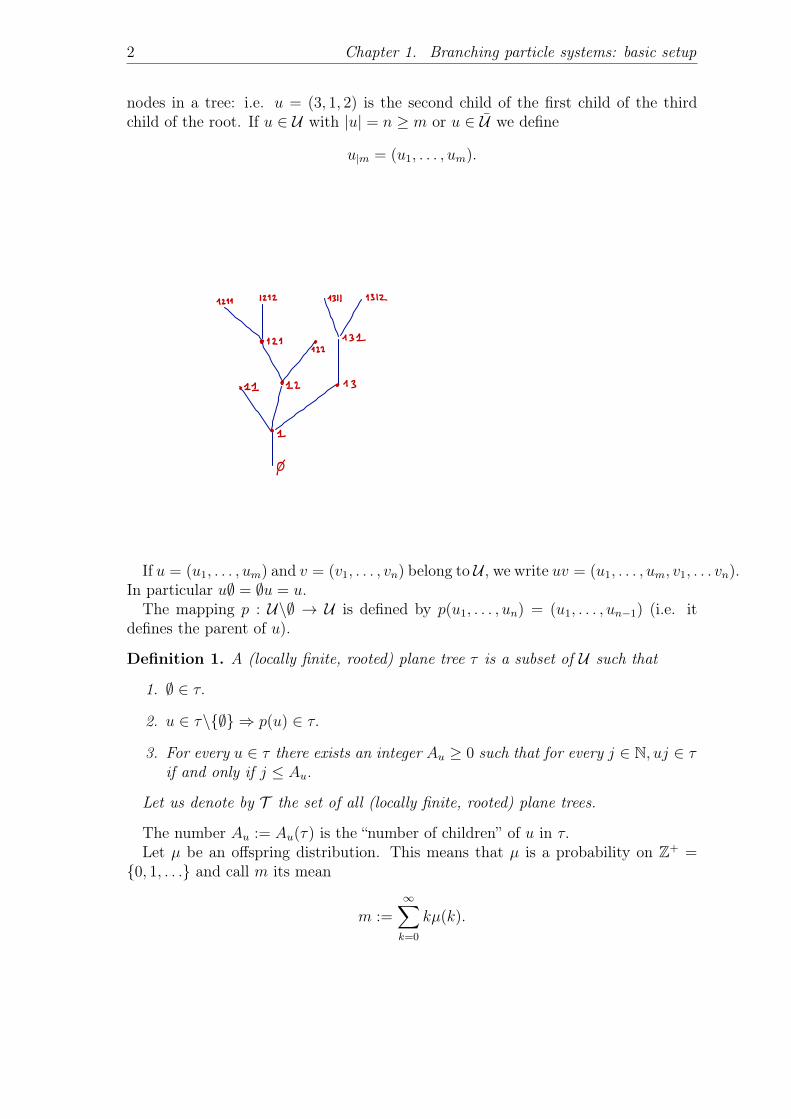
nodes in a tree: i.e. u = (3, 1, 2) is the second child of the first child of the thirdchild of the root. If u ∈ U with |u| = n ≥ m or u ∈ U we define

u|m = (u1, . . . , um).

If u = (u1, . . . , um) and v = (v1, . . . , vn) belong to U , we write uv = (u1, . . . , um, v1, . . . vn).In particular u∅ = ∅u = u.The mapping p : U\∅ → U is defined by p(u1, . . . , un) = (u1, . . . , un−1) (i.e. it

defines the parent of u).

Definition 1. A (locally finite, rooted) plane tree τ is a subset of U such that

1. ∅ ∈ τ.

2. u ∈ τ\∅ ⇒ p(u) ∈ τ.

3. For every u ∈ τ there exists an integer Au ≥ 0 such that for every j ∈ N, uj ∈ τif and only if j ≤ Au.

Let us denote by T the set of all (locally finite, rooted) plane trees.

The number Au := Au(τ) is the “number of children” of u in τ.Let µ be an offspring distribution. This means that µ is a probability on Z+ =0, 1, . . . and call m its mean

m :=∞∑k=0

kµ(k).

1.2 spatial trees 3

To define a Galton-Watson tree with offspring distribution µ, we let (Au, u ∈ U)be a collection of independent random variables with law µ indexed by the set U .Denote by T the random subset of U defined by

T = u = (u1, . . . , un) ∈ U : uj ≤ Ap(u|j), for every 1 ≤ j ≤ n.

The Galton-Watson process with reproduction law µ is a discrete time Markovprocess with values in Z+ which is defined by the recursive equation

Z0 = 1; ∀n ≥ 0, Zn+1 =Zn∑i=1

Xi,n (1.1)

where the Xi,n are i.i.d. variables with law µ.

Proposition 2. T is a.s. a tree (the Galton-Watson tree with reproduction law µ).Moreover, if

Zn = #u ∈ T : |u| = n,then (Zn, n ≥ 0) is a Galton-Watson process with offspring distribution µ and initialvalue Z0 = 1.

We denote by Pµ the law of T on T .From now on T is a µ-Galton-Watson tree, (Zn, n ≥ 0) is the assocated Galton-

Watson proces, A is a variable with law µ (i.e. an offspring variable). To avoid trivialcases we always assume µ(0) + µ(1) < 1.

1.2 spatial trees

A spatial tree is a tree τ ∈ T enriched with the following extra structure: for eachu ∈ τ we associate a life-time σu ≥ 0. For each u this allows us to define the birth-time of u by bu =

∑v<u σv and its death time du = bu + σu. Furthermore, for each

u ∈ τ there is a map Yu : R+ → E where E is the space in which particles are living.Formally, a marked tree is the triplet

t = (τ, σ, Y ) = (τ, σu, (Yu(s), s ≥ 0), u ∈ τ).

We let N (t) ⊂ U be the set of particles that are alive at time t,

N (t) := u ∈ τ : bu ≤ t < du.

For each u in N (t) we define inductively the position in E of the particle u at timet as

Xu(t) := Yu(t− bu) +Xp(u)(bu−)

where recall that Xp(u)(du) is just the position of death of the parent of u.We extend the notion of position for u ∈ N (t) to include the ancestors of u, so if

v ∈ N (s) for some s < t and v is an ancestor of u, then we set Xu(s) := Xv(s).

4 Chapter 1. Branching particle systems: basic setup

Example 3. Take τ to be the binary tree (i.e. τ = ∪n∈N1, 2n), σu = 1/|u| and

Yu(s) =

2−|u|s if last digit is 1

−2−|u|s if last digit is 2.

We call t the set of all marked trees. We are now going to define various probabilitydistributions on this space.

1.3 Dyadic branching Brownian motion

The standard branching Brownian motion (or dyadic branching Brownian motion)is obtained with the following choice:

1. Au = 2,∀u ∈ U (that is τ is the regular binary tree τ = ∪n∈N1, 2n)

2. the σu are i.i.d. with mean one exponential distribution.

3. The Yu are standard Brownian motions.

Definition 4. Writing ω = (τ, (σu, Yu)u∈τ ) we then define

X(t) = X(t, ω) = (Xu(t), u ∈ Nt)

to be the branching Brownian motion process. The natural filtration of this processis

Ft = σX(s), s ≤ t = σX(s),Ns.The law of this process is denoted by P or Px when we need to emphasize that itsinitial state is a single particle sitting at x ∈ E.The branching Brownian motion process is sometime defined as measure-valued

processµt(·) =

∑u∈Nt

δXu(t)(·)

which is also Ft-adapted but contains less information than X(t) (why?).

Remark 5. Observe that the following random variables are measurable with respectto Ft• All the σv such that v < u for some u ∈ N (t) (i.e. the life-times of particlesthat are already dead by time t)

• Any Xu(s) for s ≤ t and u ∈ N (t) (i.e. the positions of the ancestors ofparticles alive at time t)

The following proposition is is clear from the absence of memory property of ex-ponentials and the Markov property of Brownian motions.

Proposition 6. The branching Bronian motion X(t) (or µt) is strongly Markovian.

1.4 Branching random walk 5

1.4 Branching random walk

Let us now see a second example of random marked tree which will be a related butdifferent model.

A (random) point-measure Θ(·) on E is a discrete point-mass measure on E

Θ(·) =N∑i=1

δxi(·)

where N (random) is (a.s.) finite and the xi are (random) points of E.

Definition 7. A (discrete-time) branching random walk with reproduction-displacementmechanism Θ is a random marked tree such that

• τ is a Galton-Watson process with reproduction mechanism given by N =∫EdΘ

(the number of atoms in θ)

• the life-times σu are all equal to 1 (deterministic),

• For each u ∈ τ , the point process∑Au

i=1 δYu(0)(·) is an independent copy of thepoint process θ (i.e. offsprings are born at distances from the parent which aregiven by an independent copy of the point measure Θ).

• The maps s→ Yu(s) are constant (i.e. particles are born at a distance of theirparent given by Yu(0) and then don’t move).

Observe that the Yu are not necessarily independent one from another when theyhave the same parent at the previous generation.

As for the Brownian motion, we like to think about branching random walks asMarkovian processes. At each generation, each particle reproduces independently ofthe others, and the position of the offsprings relative to their parent form i.i.d. copiesof the point-measure Θ.

1.5 First properties of the dyadic branchingBrownian motion

Proposition 8.E[N(t)] = et, ∀t ≥ 0

In fact (N(t), t ≥ 0) is a pure birth process called a Yule process.

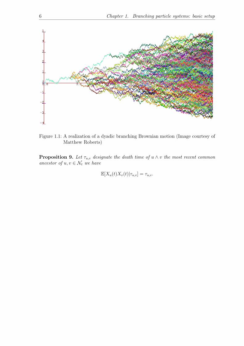
The branching Brownian motion is a cloud of particles which is growing in sizeand shape. At time t there is of order et particles and each of these particle u is at aposition Xu(t) which is a centered Gaussian variable with variance t (like a Brownianmotion). However, the Xu(t) are not independent, in fact their correlation structureis given by their genealogical history.

6 Chapter 1. Branching particle systems: basic setup

Figure 1.1: A realization of a dyadic branching Brownian motion (Image courtesy ofMatthew Roberts)

Proposition 9. Let τu,v designate the death time of u ∧ v the most recent commonancestor of u, v ∈ Nt we have

E[Xu(t)Xv(t)|τu,v] = τu,v.

Chapter 2The F-KPP equation and McKeanrepresentation

2.1 FKPP equation

The F-KPP or KPP or Kolmogorov equation is a semilinear heat equation of theform

ut =1

2uxx + g(u) (2.1)

where the forcing term g is assumed to be in C1[0, 1] and to satisfy the conditions

g(0) = g(1) = 0, g(u) > 0, u ∈ (0, 1) (2.2)

andg′(0) = β > 0, g′(u) ≤ β, u ∈ (0, 1]. (2.3)

This equation was first considered in 1937 by R.A. Fisher in The advance of ad-vantageous genes; and by Kolmogorov, Petrovsky and Piskunov Étude de l’équationde la diffusion avec croissance de la quantité de matière et son application à un prob-lème biologique. Over the years, this reaction-diffusion equation has been studied bymany authors, both probabilistically and analytcally (see Kolmogotv et al., Fisher,Skorokhod, McKean, Bramson, Neveu, Aronson and Weinberger, Harris, Kyprianouto name just some of them.)This equation is ubiquitous in the study of reaction-diffusion phenomena and front

propagation. It appears in models related to fields as diverse as ecology, populationgenetics, combustion, epidemiology, etc... It is one of the simplest example of asemilinear parabolic equation which admits traveling wave solutions (more on thislater) and its study is a very active field of research in the p.d.e. community.

The prototypical example of forcing term that we are going to consider is

g(u) = βu(1− u).

7

8 Chapter 2. The F-KPP equation and McKean representation

The case g(u) = u(1− u)2 appears naturally in the context of a genetic model forthe spread of an advantageous gene through a population. More generally, if g(u)/uis monotone decreasing then u(t, x) may be considered as the density of a populationof individuals with exponential growth near 0 and which saturates at u = 1.The Kolmogorov equation is sufficiently well behaved so that there is no difficulty

in establishing existence and unicity of the solution under measurable initial data.One may next enquire about the asymptotic behavior of solutions as t→∞.

2.2 Maximum of the BBM

Here is a first connection between the branching Brownian motion and the Kol-mogorov equation. Let X be a BBM with reproduction law (pk)k≥0 and branchingrate β (i.e. σu is exponential parameter β for each u). Let

M(t) = maxu∈Nt

Xu(t).

Theorem 10. Let u(t, x) := P0[M(t) ≤ x]. Then u satisfiesut = 1

2uxx + β(f(u)− u)

u(0, x) = 1x≥0(2.4)

where f(u) :=∑∞

k=0 pkuk.

The initial condition u(0, x) = 1x≥0 is sometimes called the Heavyside initialcondition.We are going to see two proofs of this. The first one although slightly informal

could be made rigorous with little effort.

Proof. For simplicity we assume that β = 1 and p2 = 1 (dyadic case). We want tocompute u(t+ dt, x)− u(t, x) up to terms of order dt where dt is small. The idea isto decompose according to what happen to the branching Brownian motion in theinitial interval [0, dt] of time.

• With probability (1 − dt) + o( dt) it doesn’t branch and conditionally to thisevent

P[M(t+ dt) ≤ x] = P[M(t) ≤ x−Bdt] = u(t, x−Bdt)

where B is a Brownian motion.

• With probability dt + o( dt) there is exactly one branching event and condi-tionally to this event

P[M(t+ dt) ≤ x] = (P[M(t) ≤ x−Bdt])(P[M(t) ≤ x−B′dt]) = (P[M(t) ≤ x])2+o(1)

where B and B′ are correlated Brownian motions.

2.3 McKean representation 9

Thus

P[M(t+ dt) ≤ x]− P[M(t) ≤ x] = (1− dt)P[M(t) ≤ x−Bdt] + dtu2(t, x) + o( dt)− u(t, x)

= [E(u(t, x−B dt))− u(t, x)] + dt[u2(t, x)− u(t, x)] + o( dt)

where in the last line we have absorbed the term dt× (u(t, x−Bdt)− u(t, x)) in theo( dt) term. Recall that if g is a smooth enough function, then v(t, x) = Ex[g(Bt)]solve the heat equation vt = 1

2vxx. Thus, writing g(z) = u(t, z) we see that

E[u(t, x−Bdt)] = Ex[g(Bdt)]

and thereforelimdt→0

E(u(t, x−Bdt))− u(t, x)

dt=

∂2

∂x2u(x, t).

Hencelimdt→0

u(t+ dt, x)− u(t, x)

dt=

∂2

∂x2u(x, t) + [u2(t, x)− u(t, x)].

Unless specified otherwise, we will consider the following version of the FKPP equa-tion. recall that f(s) = E(sA) is the generating function of the offspring distribution.We pick a non-linear term g which as follows

∂u

∂t=

1

2

∂2u

∂x2+ β(f(u)− u). (2.5)

In the special case where the branching is dyadic this becomes

∂u

∂t=

1

2

∂2u

∂x2+ β(u2 − u). (2.6)

2.3 McKean representation

The following Theorem, due to McKean, 1975 [24], gives a representation of solutionsto the F-KPP equation (2.5) in term of the BBM.

We will need to deal with functionals of the BBM which can be expressed in termsof functions of the position of the particles at time t. Thus, we would like to be ableto tell when such a functional is a martingale. This is very easy once we write downthe generator.For now, let us look at the BBM as a Markov process in the state space

S := ∪n∈N(n × Rn

),

Consider functions F : R+ × S 7→ R, F (t, n, x) = F (t, n, (x1, . . . , xn)) which are C2

in the space variables. Of course, the second argument of F being the dimensionof x the third argument, it is completely redundant and is written only for the sakeof clarity. We write xi = (x1, x2 . . . , xi, xi, . . . xn) for the vector obtained from x byrepeating once the i-th coordinate.For simplicity, we continue to restrict ourselves to the case of the dyadic branching

Brownian motion.

10 Chapter 2. The F-KPP equation and McKean representation

Theorem 11. The dyadic branching brownian motion with branching rate β > 0 isFellerian and its generator is

GF (t, n, x) :=n∑i=1

1

2

∂2

∂x2i

F (t, n, x) +n∑i=1

β[F (t, n+ 1, xi)− F (t, n, x)]

The following is classical:

Proposition 12. If F : [0,∞)× S 7→ R is C1,2 in t and x respectively and(G +

∂

∂t

)F ≡ 0 (2.7)

then (F (t,#Nt, X(t)), t ≥ 0) is a local martingale.

The next Theorem is often called the McKean representation. It says that solutionsof the FKPP equation can be viewed as an expectation with respect to the BBM. Itis at heart a Feynman-Kac type of result.

Theorem 13. If u : R+ × R 7→ R satisfies u ∈ [0, 1] and solves the FKPP equationwith initial condition g

∂u∂t

= 12∂2u∂x2 + β(f(u)− u)

u(0, x) = g(x)(2.8)

then u has the representation

u(t, x) = Ex

[∏u∈Nt

g(Xu(t))

]. (2.9)

Proof. Suppose u satisfies the FKPP equation (2.8). Then it is easily checked thatthe function

F (s,X(s)) :=∏u∈Ns

u(t− s,Xu(s)), s ≤ t

satisifies the condition of Proposition 12 and is thus a local martingale. But sinceu ∈ (0, 1) it is bounded and is thus a true martingale. We conclude that

u(t, x) = Ex[F (0, X(0))] = Ex(F (t,X(t))) = Ex

[∏u∈Nt

g(Xu(t))

]which is the McKean representation.

Indeed (let’s check this easily checkable fact)

GF (s,X(s)) =∑u∈Ns

∏v 6=u

u(t− s,Xv(s))∂2

∂x2(t− s,Xu(s))

+∑u∈Ns

F (s,X(s))(u(t− s,Xu(s))− 1)

2.3 McKean representation 11

while

∂

∂tF (s,X(s)) = −

[ ∑u∈Ns

∏v 6=u

u(t− s,Xv(s)) ∂2

∂x2u(t− s,Xu(s))

+ (u2(t− s,Xu(s))− u(t− s,X − u(s)))]

which are the same up to the minus sign.

Chapter 3Position of the rightmost particle

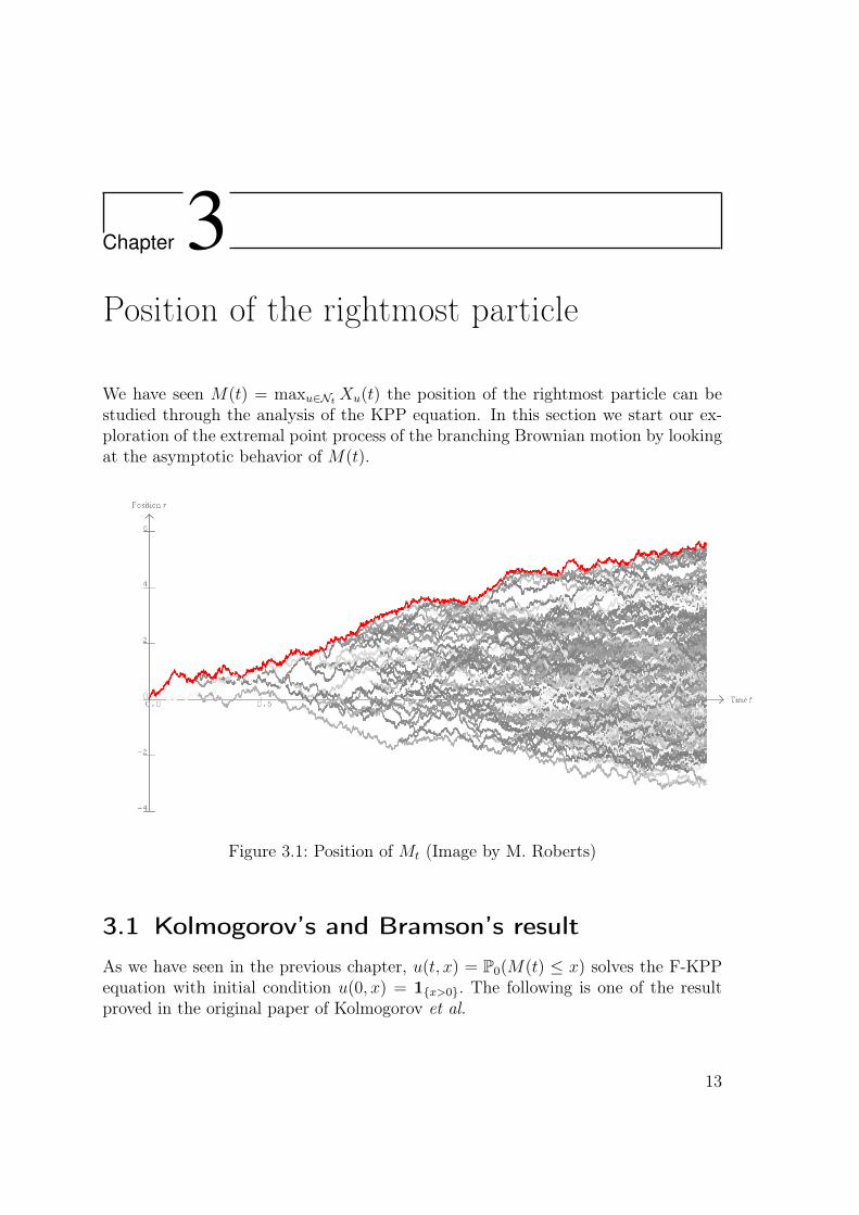
We have seen M(t) = maxu∈Nt Xu(t) the position of the rightmost particle can bestudied through the analysis of the KPP equation. In this section we start our ex-ploration of the extremal point process of the branching Brownian motion by lookingat the asymptotic behavior of M(t).

Introduction The maximal particle

Some notation

We want to know about the position of the maximal (top-most) particle inthis picture.

Let N(t) be the set of particles alive at time t.

For u ∈ N(t) and s ≤ t, let Xu(s) be the position of the unique ancestor of uthat was alive at time s.

Define Mt = maxu∈N(t) Xu(t).

Matt Roberts mattiroberts@gmail.com (McGill) Asymptotics for the frontier of BBM 9th September, 2011 5 / 16Figure 3.1: Position of Mt (Image by M. Roberts)

3.1 Kolmogorov’s and Bramson’s result

As we have seen in the previous chapter, u(t, x) = P0(M(t) ≤ x) solves the F-KPPequation with initial condition u(0, x) = 1x>0. The following is one of the resultproved in the original paper of Kolmogorov et al.

13

14 Chapter 3. Position of the rightmost particle

Theorem 14 (Kolmogorov, Petrovski and Piskunov, 1937). There exists a mapt 7→ mt such that

u(t,mt + x)→ w(x) uniformly in x ∈ R as t→∞

where w solves1

2w′′ +

√2w′ + w(w − 1) = 0. (3.1)

check sign of nonlinearity Furthermore, mt =√

2t+ o(t)

Remark 15. Observe that this says that M(t) − mt converges in distribution to avariable whose cumulative distribution function is given by w.

Any function w that solves (3.1) is called a traveling wave solution of (2.1) withspeed

√2 since it is ealy checked that then

u(t, x) = w(x−√

2t)

is a solution of (2.1). More generally, if wλ solves

1

2w′′ + λw′ + w(w − 1) = 0. (3.2)

thenu(t, x) = w(x− λt)

is also a solution. wλ is a traveling wave solution with speed λ. The terminologycomes from the fact that the fixed shape front wλ is traveling at constant speed λ.Kolmogorov et al. also show that traveling waves exist for all λ such that λ ≥

√2

and that for each such λ the solutions of (3.2) are unique up to an additive constantin the argument (i.e. if wλ is solution, so is wλ(·+ k)). We will come back to this insection 5.This result was greatly improved upon by Bramson in two steps, first in 1978 and

then in 1983. He showed that

Theorem 16 ([7] Bramson, 1983). For all initial condition u(0, x) = g(x) increasingsufficiently fast1 (including the Heaviside initial condition) then

u(t, x+mt)→ w(x) uniformly in x ∈ R as t→∞ (3.3)

where mt =√

2t 32√

2log t+ C + o(1)

Remark 17. In particular this means that we can choose mt =√

2t− 3 · 2−3/2 log tin the convergence (3.3). The constant C in mt depends on the precise shift of wwhich is chosen.

We will also show that

Theorem 18. Almost surely, limt→∞Mt

t=√

2 and limt→∞Mt −√

2t = −∞.1This will be made precise later

3.2 First moment calculations 15

3.2 First moment calculations

Let us look at a first moment argument and see if we can obtain the first order ofthe position of the rightmost particle, i.e Mt ∼

√2t.

I want to determine a value c > 0 which is critical for P(∃u ∈ N (t) : Xu(t) > ct).The following bound for the tail distribution of a Gaussian variable is classical and

will be used repeatedly in the following

Exercise 19. Show that

e−x2/2

√2π

(1

x− 1

x3

)≤ 1√

2π

∫ ∞x

e−y2/2 dy ≤ e−x

2/2

x√

2π. (3.4)

Using the linearity of expectation and (3.4) we see that

P(∃u ∈ N (t) : Xu(t) > ct) ≤ E[ ∑u∈N (t)

1Xu(t)>ct]

= etP[B(t) > ct]

≤ ete−c

2t/2

ct1/2√

2π= et(1−c

2/2) 1

ct1/2√

2π

which tends to 0 as soon as c ≥√

2 and

E[ ∑u∈N (t)

1Xu(t)>ct]≥ et(1−c

2/2) 1√2π

(1

ct1/2− 1

c3t3/2).

which tends to infinity as soon as c <√

2. So if we can show that this expectation“doesn’t lie”, i.e. that it is not dominated by rare events in which we have massivenumber of particles above ct then we should be able to show that c =

√2. This is

what we are going to do in this section.Observe first that Kingman’s ergodic subadditive theorem implies that Mn/n→ c

for some finite constant. develop

3.3 Warm up: the independent case

It will be instructive to start by looking at the following simpler case. Supposethat (Xu, u ∈ U) is a collection of independent Brownian motions, and that Ntis the population at time t of a branching Brownian motion. Let us call Mt :=maxXu(t), u ∈ Nt the maximum of N(t) := #Nt independent Gaussian variableswith the same variances as the Xu(t).Remember that (N(t), t ≥ 0) is a Yule process and that it is known that Z(t) =

e−tN(t) is a (positive) martingale which converges almost surely and in L1 to a limitZ which is furthermore an exponential variable with mean 1. We are going to showthe following

16 Chapter 3. Position of the rightmost particle

Proposition 20.

P(Mt ≤ mt + x)→ w(x) = E[e−cZe

−√

2x]where mt =

√2t− 1

2√

2log t and Z is the almost sure limit of the martingale e−tN(t).

Remark 21. This proves the convergence in distribution of Mt − mt

Proof. The estimate (3.4) implies that for any at = o(t1/2)

P(X(t) >√

2t− at) = P(t−1/2 >√

2t− at/t1/2) ∼ 1√4πt−1/2e−t+

√2at+o(1)

so by choosing at = 12√

2log t− x we have that

P(X(t) >√

2t− 1

2√

2log t+ x) ∼ ce−te−

√2x.

Thus,

P(Mt ≤ mt + x

)= P

(∀u ∈ Nt : Xu(t) ≤ mt + x

)= E

[(1− P(X(t) > mt + x))#Nt

]= E

[(1− ce−te−

√2x(1 + ot(1)))e

tZ(1+ot(1))]

where Z is the limit of the martingale Z(t) := e−t#Nt and is an exponential meanone variable. Finally we conclude that

P(Mt ≤ mt + x

)∼t→∞ E

[exp

− cZe−

√2x].

Remark 22. Observe that the tail of Mt − mt is doubly exponential to the left andexponential to the right. This asymmetry is typical of Gumbel variables.

What we are now going to show is a similar Theorem for M(t)

Theorem 23. Take mt =√

2t− 32√

2log t, then M(t)−mt converges in distribution

and there exists a random variable Z such that

limt→∞

P(M(t) ≤ mt + y) = E[

exp(−cZe−√

2y)]

3.4 A first attempt at the moments method for the law of large numbers 17

3.4 A first attempt at the moments method for thelaw of large numbers

Looking in more details at the first moment argument above we see that we caneasily get an upper bound out of it. Indeed, for each ε > 0 we can find c(ε) > 0 suchthat

P(∃u ∈ N (t) : Xu(t) > (1 + ε)√

2t) ≤ e−c(ε)t

for t large enough. Thus, we conclude (with Borel Cantelli) that for any fixed δ > 0

lim supn

Mnδ

nδ≤√

2

This easily implies that lim suptMt

t≤√

2 (do it!).

What would be the natural approach for the lower bound? One might want todefine

Z(t) :=∑u∈Nt

1Xu(t)>(1−ε)√

2t

and show that with high probability Z(t) > 1. To do this the classical tool is thesecond moment method. Given a N-valued random variable Z

E(Z) = E(Z1Z≥1) ≤ E(Z2)1/2P(Z ≥ 1)1/2

so thatP(Z ≥ 1) ≥ (EZ)2

E(Z2).

Now, in the cases where we have independent Gaussian variables, as in the warm-up, we have that

P(Mt ≥ (1− ε)√

2t) ≥ e2tP(X(t) ≥ (1− ε)√

2t)2

E(∑

u,v∈Nt 1Xu(t)>(1ε)√

2t 1Xv(t)>(1−ε)√

2t)

=e2tP(X(t) ≥ (1− ε)

√2t)2

etP(X(t) ≥ (1− ε)√

2t) + E[Nt(Nt − 1)]P(X(t) ≥ (1− ε)√

2t)2

Recall that E[Nt(Nt − 1)] = e2t − 2et and that for each ε > 0 there exist c(ε) > 0such that

etP(X(t) ≥ (1− ε)√

2t) ≥ ec(ε)t

we see thatP(Mt ≥ (1− ε)

√2t) ≥ 1

e2t−2et

e2t+ e−c(ε)t

≥ 1− e−c′(ε)t

which implies that

lim inft

Mt

t≥√

2.

18 Chapter 3. Position of the rightmost particle

This line of reasoning fails when we try it with Mt. The reason is that in this caseE[∑

u,v∈Nt 1Xu(t)≥(1−ε)√

2t1Xv(t)≥(1−ε)√

2t] is much larger due to correlations.Here is a “back of the envelope” calculation that should help convince you: Let us

call G the number of particles near λt at time t (with λ > 0). Because the cost fora Brownian motion to get to λt is e−

λ2

2t we have that

E[G] ≈ et−λ2

2t.

Now we want to consider E[G2] which is the expectation of the number of pairs ofparticles near λt at time t. We do a violent lower bound

E[G2] ≥ E[# pairs of particles near λt whose last common ancestor was near2

3λt at time

t

2]

= E[∑w∈Nt

1Xw(t/2)≈ 23λ t

2

∑u∧v=wu,v∈Nt

1Xu(t)=λt 1Xv(t)=λt]

≈ et/2−12

( 43λ2) t

2 ×(et2− 1

2( 2

3λ)2 t

2

)2

= e32t− 2

3λ2t

which means that if λ >√

32, then E[G2] E[G]2.

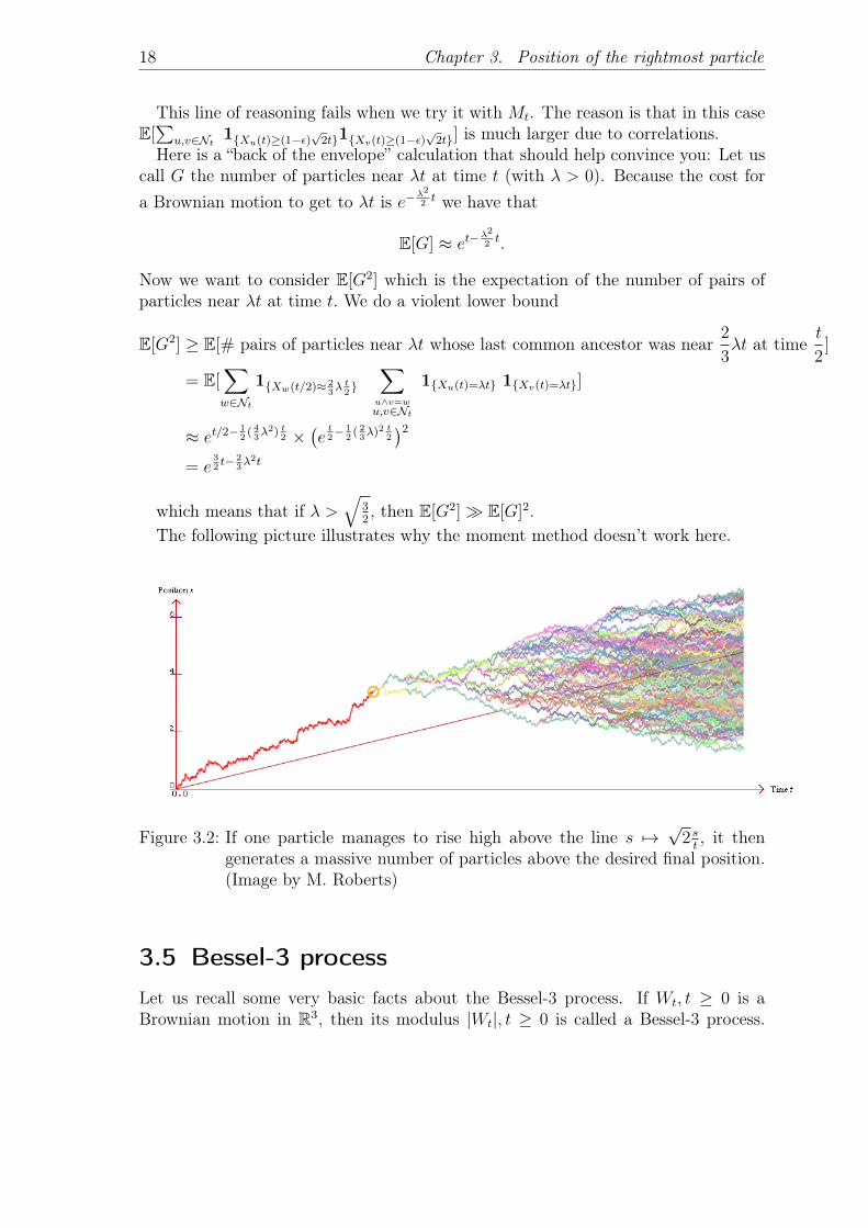
The following picture illustrates why the moment method doesn’t work here.

A new proof of Bramson’s theorem The expected number of particles

The expected number of particles above βt

Let β =√

2 − 32√

2

log tt + y

t .

E[#u ∈ N(t) : Xu(t) > βt] = etP(Bt > βt) ≈ te−√

2y .

But this is bigger than we hoped. . . what’s going wrong?

Matt Roberts mattiroberts@gmail.com (McGill) Asymptotics for the frontier of BBM 9th September, 2011 7 / 16

Figure 3.2: If one particle manages to rise high above the line s 7→√

2 st, it then

generates a massive number of particles above the desired final position.(Image by M. Roberts)

3.5 Bessel-3 process

Let us recall some very basic facts about the Bessel-3 process. If Wt, t ≥ 0 is aBrownian motion in R3, then its modulus |Wt|, t ≥ 0 is called a Bessel-3 process.

3.6 The many-to-one Lemma 19

Suppose that Bt, t ≥ 0 is a Brownian motion in R started from B0 = x under Px:then

ζt :=Bt

x1Bs>0,∀s≤t

is a non-negative, mean one martingale under Px, so we can define a new probabilitymeasure Qx by

dQx

dPx

∣∣Gt

:= ζt

where Gt is the natural filtration of Bt. Then Bt; t ≥ 0 is a Bessel process startedfrom x under Qx. The density of a Bessel process satisfies

Qx(Bt ∈ dz) =z

x√

2πt

(e−(z−x)2/2t − e−(z+x)2/2t

)dz

and it can be checked that

Qx(·) = limt→∞

Px(·|τ0 ≥ t) = Px(·|τ0 =∞)

where τ0 = inft : Bt = 0 (the Bessel process is a Brownian motion conditioned tonever hit 0).

The following estimate for the density of a Bessel is going to be crucial.

Exercise 24 (Estimate for the density of a Bessel process). For any x, z = o(√t)

Qx(Bt ∈ dz) ∼√

2

π

z2

t3/2.

as t→∞.

3.6 The many-to-one Lemma

The many-to-one Lemma is a simple and well known tool in branching processes.

Lemma 25 (Many-to-one Lemma (1st version)). For any t ≥ 0, for any measurablefunction F : C[0,t] 7→ R we have

E[∑u∈N(t)

F (Xu(s), 0 ≤ s ≤ t)] = etE[F (Bs, 0 ≤ s ≤ t)].

where Bs is simply a standard Brownian motion under P.

The proof is straightforward as this is simply the independence of the particlestrajectories and the branching history coupled with the linearity of the expectation.

Examples of functionals we may want to look at are

F (X(s), s ≤ t) = 1X(t)≥x, F (X(s), s ≤ t) = 1X(s)≥x∀s≤t, F (X(s), s ≤ t) = t2e∫ t0 X(s) ds.

20 Chapter 3. Position of the rightmost particle

Suppose now that we are given a curve f : [0,∞)→ R, f ∈ C2 such that f(0) = 0and we want to compute

E[∑u∈Nt

F (Xu(s), s ≤ t)1Xu(s)<α+f(s),∀s≤t]

where α > 0 s fixed. Observe that the summands are again just path functionals ofthe Xu. If we wanted a Brownian particle B to follow f we would apply the usualGirsanov martingale transform

gt = e∫ t0 f′(s) dBs−

∫ t0 (f ′(s))2 ds

i.e. under Pf defined by dPf/ dP |Gt = gt the process Bt := α + f(t) − Bt is aBrownian motion started from α. Let us now do a further change of measure anddefine a new probability Q by

dQ

dPf

∣∣Ft

=Bt

α1Bs>0∀s≤t

then B is a Bessel-3 process under Q started from α.Combining the many-to-one Lemma with these two changes of measure we get

that for a path-functional F

Lemma 26. Let ζ(t) := 1α

(α+ f(t)−Bt)e∫ t0 f′(s) dBs−

∫ t0 (f ′(s))2 ds1Bs≤α+f(s),s≤t. Then

E[∑x∈Nt

F (Xu(s), s ≤ t)1Xu(s)≤α+f(s),s≤t] = etQ[1

ζ(t)F (Bs)]

where under Q, Bt = α + f(t)−Bt, t ≥ 0 is a Bessel process.

3.7 M. Roberts’ “simple path”

We are now going to follow Matthew Roberts recent paper [28] and some develop-ments from Zeitouni’s lecture notes to obtain Theorem 23 which is part of Bramson’sresults.The main idea is that in order to avoid the second moment problem we are going

to count only the particles that stay below a certain line.

3.7.1 Bounds on the tail of M(t)

Letβ :=

√2− 3

2√

2

log t

t(3.5)

and define

H(y, t) := #u ∈ Nt : Xu(s) ≤ βs+ 1 ∀s ≤ t, βt+ y − 1 ≤ Xu(t) ≤ βt+ y (3.6)

3.7 M. Roberts’ “simple path” 21

Lemma 27 (First moment for H). For t ≥ 1 and y ∈ [0,√t]

E[H(y, t)] e−√

2t.

Proof. We apply our many to one Lemma for counting particles staying under acurve with f(s) = βs and α = 1 to obtain

E[H(y, t)] = etQ[ 1

ζ(t)1βt+y−1≤Bt≤βt+y

]= etQ

[ye−βBt+β2t/2

βt+ y − Bt1βt+y−1≤Bt≤βt+y

] yet−β

2t/2Q[βt+ y − 1 ≤ Bt ≤ βt+ y]

yt3/2e−√

2y Q[1 ≤ βt+ y + 1−Bt ≤ 2].

Since βt+ 1−Bt is a Bessel under Q we have that

Q(1 ≤ βt+ y + 1−Bt ≤ 2) ∫ 2

1

z2

t3/2dz t−3/2.

We sketch the rest of the proof. Roberts then use a many-to-two Lemma to provethat there exists a constant such that

E[H(y, t)2] ≤ cE[H(y, t)]

and from there the second moment method allows us to conclude that

P(H(y, t) 6= 0) ≥ c′ye−√

2y.

this gives us a lower bound for m1/2(t).

For the upper bound, Roberts use a similar technique. Let us introduce the fol-lowing set Γ which has almost the same definition as H

Γ = #u ∈ Nt : Xu(s) ≤ f(s)∀s ≤ t, βt+ y − 1 ≤ Xu(t) ≤ βt+ y

where now

f(s) =

βs+ y + 3

2√

2log(s+ 1) if s ≤ t/2

βs+ y + 32√

2log(t− s+ 1) if t/2 ≤ s ≤ t

Using the same type of calculations (albeit more involved) as above, Roberts showsthat

E[Γ] ≤ c(y + 2)4e−√

2y.

22 Chapter 3. Position of the rightmost particle

Interestingly, we don’t need a second moment here (as we are going for an upperbound). Instead we are going to estimate the probability that a particle cross ourcurve f(s) before time t. Let’s call τ the first time a particle crosses f(s). Robertsshows that there exists a constant c such that

P(τ < t) ≤ c(y + 2)4e−√

2y.

To see this, it is enough to show that

E[Γ|τ < t] ≥ c′

for some constant c′ > 0, i.e. that once we hit f(s) the hard work is done and wewill have particles ending up near βt+ y. Thus

P(τ < t) ≤ E[Γ]P(τ < t)

E[Γ1τ<t]=

E[Γ]

E[Γ|τ < t]≤ c1

c2

(y + 2)4e−√

2y.

By Markov inequality this implies

P(M(t) ≥√

2t− 3

2√

2log t+ y) ≤ P(Γ ≥ 1) + P(τ < t) ≤ c(y + 2)4e−

√2y

for some c > 0.

3.7.2 Result about E[M(t)] and the median

Proposition 28. The median m1/2(t) of M(t) satisfies

m1/2(t) =√

2t− 3

2√

2log t+O(1) as t→∞.

Proof. To summarize what we have learned in the previous section : we now knowthat there are two constants c, c′ such that for 0 ≤ y ≤

√t,

ce−√

2t ≤ P(Mt >√

2t− 3

2√

2log t+ y) ≤ c′(y + 2)4e−

√2t. (3.7)

Define mδ(t) := infx : P(M(t) > x) ≤ δ. Then, by choosing δ small enough theabove implies that

mδ(t) =√

2t− 3

2√

2log t+O(1).

Let us show quickly thatM(t)−mδ(t) is tight which is enough to yield the desiredconclusion. Fix ε > 0 and choose L such that

E[(1− δ)−N(L)] < ε/2

and then a such thatP(min

u∈NtXu(t) < −a) < ε/2.

3.8 Convergence in law of M(t)−mt. 23

For a particle u ∈ NL and t > L note as usual M (u)t the position of the maximal

descendent of u at time t. Then

P(M(t) ≤ mδ(t− L)− a)

≤ P(minu∈Nt

Xu(t) < −a) + P(minu∈Nt

Xu(t) ≥ −a,maxu∈NL

M(u)t < mδ(t− L)− a)

≤ P(minu∈Nt

Xu(t) < −a) + E[P(M(t− L) < mδ(t− L))N(L)]

≤ ε/2 + ε/2 = ε.

Observe that the upper bound implies that

E[M(t)] ≤√

2t− 3

2√

2log t+O(1).

A matching lower bound can be obtained provided we show that

limz→−∞

lim supt→∞

∫ z

−∞P(Mt ≤ mt + y) dy.

This is the approach take in Zeitouni’s lecture notes to obtain

Proposition 29.

E[M(t)] =√

2t− 3

2√

2log t+O(1) as t→∞.

3.8 Convergence in law of M(t)−mt.

3.8.1 An exact equivalent for the tail of M(t)

The first step is to reinforce the bounds

ce−√

2t ≤ P(Mt >√

2t− 3

2√

2log t+ y) ≤ c′(y + 2)4e−

√2t

into the following asymptotic equivalent:

Lemma 30. Remember that mt =√

2t − 32√

2log t. There exists a constant c such

thatP(M(t) > mt + y) ∼ cye−

√2y, as y →∞.

Proof. We only sketch the proof here.

24 Chapter 3. Position of the rightmost particle

3.8.2 Convergence of M(t)−mt

Write Mt = M(t)−mt. Then

P(Mt ≤ y) = E[P(Mt ≤ y|Fs)]= E[

∏u∈Ns

P(Mut−s ≤ mt + y −Xu(s)|Xu(s))]

= E[∏u∈Ns

(1− P(Mut−s > mt−s + y − (Xu(s)−

√2s) + o(1)|Xu(s))]

where we use that mt = mt−s +√

2s+ o(1).With probability tending to one, Ms −

√2s→ −∞ (this is Kolmogorov result, it

can also be shown directly with martingale techniques, so that y−(Xu(s)−√

2s) 1for all u ∈ Ns and hence we can use our tail estimate to obtain

P(Mt ≤ y) ∼t E[ ∏u∈Ns

(1− c(y +√

2s−Xu(s))e−√

2(y+√

2s−Xu(s))]

∼s E[

exp(−cZse−√

2y)]

where, in the last line, we have used the notation

Zs :=∑u∈Ns

(√

2s−Xu(s))e−√

2(√

2s−Xu(s)).

We have shown that

limt→∞

P(M(t)−mt ≤ y) ∼ E[exp(−cZse−√

2y)] as s→∞.

However, the left-hand side does not depends on s and hence the right hand sidemust have a limit when s → ∞. This implies that Zs → Z in distribution (Z can’tdegenerate because of a priori bounds). We conclude that

P(M(t)−mt ≤ y)→ E[

exp(−cZe−√

2y)].

Remark 31. Observe that the same argument shows that

limtP(M(t) ≤ y|Fs) = exp(−cZse−

√2y)

but that we can’t then take a limit in s on both side.

Chapter 4Spines, martingales and probabilitychanges

Spine decompositions and their relation to probability tilting for branching processesis one of these ideas that have discovered several time by different group of peopleunder different guises. One should however certainly credit the 1998 Paper of Lyons,Pemantle and Peres for bringing it in sharper focus. It is a tool that has since beenused with great efficiency by people like Kyprianou, Harris, Roberts, etc...

The idea is that we are going to distinguish one particular line of descent from theroot, so at each time there will be a tagged particle that we will call the spine. Once wehave enlarged our probability space to take this extra-information into account thishelps tremendously to simplify the probability tilting method pioneered by Chauvinand Rouault.

4.1 Dyadic Brownian motion with spine

Definition 32. A spatial tree with a spine is a pair (t, ξ) where t = (τ, σ, Y ) is aspatial tree and ξ is a subset of U with the following properties

1.#ξ ∩N (t) ≤ 1,∀t ≥ 0

2. u ∈ ξ ⇒ v ∈ ξ for each v < u.

The space of marked trees with spines is denoted by T ∗. In other words, a spineis a distinguished line of descent in a tree, finite or infinite. If v ∈ ξ ∩ N(t) wewrite ξt = v for the label of the spine and Ξ(t) = Xξt(t) for the position of the spineparticle.

Let us now define, as simply as we can, a law P on T ∗ such that if the pair (t, ξ)has law P then t is a dyadic Brownian motion.

25

26 Chapter 4. Spines, martingales and probability changes

Definition 33. Let t be a dyadic Brownian motion with law P. Then conditionallyon t construct inductively ξ as follows. For all t < d∅ let ξt = ∅. Pick U1 uniformlyamong the offsprings of ∅ and for all t ∈ [d∅, dU1) let ξt = U1, then ξt becomes achildren of U1 picked uniformly at random, U2 and so on . . . . The law of the pairt∗ = (t, ξ) is denoted by P (or Px to emphasize the starting point).

As for the Brownian motion, we think of (X(t), ξ(t))t≥0 as the process version oft∗ and we call Ft its natural filtration. Observe that Ft ⊂ Ft. We further introduce

Gt = σ(Ξ(s), s ≤ t), t ≥ 0

the natural filtration of Ξ and

Gt = σ(Ξ(s), s ≤ t) ∨ σ(σu, u < ξt), t ≥ 0

which is G augmented with the information of the branching times along ξ.

The following simple proposition tells us that one can instead chose to first decidethe trajectory of the spine (Ξ(t), t ≥ 0) and then immigrate normal BBM on thisspine.

Proposition 34 (Spine decomposition). Let Ξ(t), t ≥ 0 be a standard Brownianmotion, let π = (t1, t2, . . .) be a rate 1 Poisson point process on R+. At each timeti a new particle is created along the spine at Ξ(ti). The label of Ξ before the splitis ξti− and ξti is obtained by appending “1” or “2” at the end with probability 1/2.The new non-spine particle starts a new independent dyadic branching Brownianmotion (without spine) shifted by time, space and label. The law of the object createdt∗ = (t, ξ) is again P.

We now make a couple of observations which will be useful later and illustratesthe use of our notations.First observe that

P(u ∈ ξ ∩Nt|Ft) = 1u∈Nt∏v<u

1

Av= 1u∈Nt2

−|u|,

where the last equality is because we are restricting ourselves to the dyadic case.We begin with the following useful Lemma

Lemma 35. If Y is an Ft-measurable random variable, then we can write

Y =∑u∈Nt

Yu1ξt=u

where each Yu is Ft-measurable.

4.2 The many-to-one Lemma 27

Proof. This is essentially a consequence of the fact that if Y ∈ Ft then there existsa measurable map F : U × T → R such that

Y = F (ξt, tt)

where tt = (X(s), s ≤ t) is all the information in t available at time t. Thus we havethat

Y =∑u∈Nt

F (u, tt)1ξt=u

and clearly Yu = F (u, tt) is Ft-measurable.

The expectation under P of a variable Y ∈ Ft can therefore be related to expecta-tions under P of its decomposition.

Definition 36. Let Y ∈ Ft have decomposition Y =∑

u∈Nt F (u, tt)1ξt=u. Then

P[Y ] = P

∑u∈N(t)

Yu∏v<u

1

Av

= P

∑u∈N(t)

Yu2−|u|

. (4.1)

4.2 The many-to-one Lemma

The following elementary result (of which more general versions will be given later)will be used repeatedly.

Lemma 37 (Many-to-one Lemma (1st version)). For any t ≥ 0, for any functionF : C[0,t] 7→ R we have

E[∑u∈N(t)

F (Xu(s), 0 ≤ s ≤ t)] = etE[F (Ξ(s), 0 ≤ s ≤ t)].

Proof.

E[∑u∈N(t)

F (Xu(s), 0 ≤ s ≤ t)] = E[E[∑u∈N(t)

F (Xu(s), 0 ≤ s ≤ t)|#N(t)]]

= E[#N(t)E[F (Ξ(s), 0 ≤ s ≤ t)]]

= etE[F (Ξ(s), 0 ≤ s ≤ t)]

Remark 38. It is clear that if branching happens at rate β and instead of dyadicbranching each splitting produce an i.i.d. number according to some random variableA with E(A) = 1 +m then the formula becomes

E[∑u∈N(t)

F (Xu(s), 0 ≤ s ≤ t)] = emβtE[F (Ξ(s), 0 ≤ s ≤ t)]

28 Chapter 4. Spines, martingales and probability changes

In particular this lemma can be applied for functions of the form F (Xu(s), 0 ≤s ≤ t) = f(Xu(t)).A slightly more general version can be formulated as follows

Lemma 39 (Many-to-one Lemma (2nd version)). For any t ≥ 0, and a variableY ∈ Ft with decomposition Y = Yξ =

∑u∈N(t) 1ξt=uYu we have

E[∑u∈Nt

Yu] = E[Yξ∏u<ξt

Au] = E[Yξt2|ξt|]

Proof.

E[Yξ∏u<ξt

Au] = E[∑u∈Nt

Yu1ξt=u(∏v<u

Av)]

= E[ ∑u∈Nt

YuP(ξt = u|Ft)(∏v<u

Av)]

= E[∑u∈Nt

Yu]

4.3 Additive martingales

The many-to-one Lemma is useful to construct martingales. Given a functional ofcontinuous paths F : t, C[0,t) → R, (x(s), s ≤ t) 7→ F [(x(s), s ≤ t)] let us define thequantities

ζ(t) := F(Ξ(s), s ≤ t

)ζu(t) := F

(Xu(s), s ≤ t

)for u ∈ Nt

Z(t) := e−t∑u∈Nt

ζu(t).

Observe that Z is Ft-adapted and that ζ is Gt adapted (it’s a Brownian functional).

Proposition 40. If ζ is a Gt-martingale, then Z is an Ft-martingale.

Remark 41. It can be shown that this is in fact an equivalence.

Proof. For u ∈ Nt let us write Fu for the functional

Fu(f(r), r ≤ s

)= F

(φ(r), r ≤ t+ s

)where

φ(r) =

Xu(r) if r ≤ t

Xu(t) + f(r − t) if r > t

4.3 Additive martingales 29

Suppose first that ζ(t) is a Gt martingale. Then

E[e−(t+s)

∑v∈Nt+s

ζv(t+ s)∣∣Ft] = e−t

∑u∈Nt

ζu(t)E[e−s

∑u≤v∈Nt+s

Fu(Xv(t+ r), r ≤ s)

ξu(t)

∣∣Ft]= e−t

∑u∈Nt

ζu(t)E[Fu(Ξ(r), r ≤ s)

ξu(t)

∣∣Ft]= e−t

∑u∈Nt

ζu(t)

where we have used that conditionally on Ft, each particle u ∈ Nt starts an inde-pendent BBM from its position for which we can apply the many-to-one Lemma.The last line is just the property that ζ being a martingale, its expectation staysconstant. Thus we have shown that Z is an Ft martingale.

The case where F depends only on the current position is particularly simple

Proposition 42. Let h : R 7→ R be a C2 function, then

W (t) :=∑u∈N(t)

h(Xu(t) + ct), t ≥ 0

is a local Ft-martingale if and only if h solves

1

2h′′ + ch′ + h = 0. (4.2)

Equation (4.2) will appear again as the linearized version off the so-called KPPtraveling wave equation.

Example 43 (Exponential additive martingales). For λ ∈ R we define

Wλ(t) :=∑u∈N(t)

e−λ(Xu(t)+cλt) (4.3)

for t ≥ 0, λ ≥ 0 and with cλ = λ/2 + mβ/λ. Then the process (Wλ(t), t ≥ 0) is amartingale.

Proof. It suffices to observe that e−mβte−λ(ξt+cλt) = e−λξt−λ2

2t is a Brownian martin-

gale.

Remark 44. Wλ is clearly a positive martingale and therefore Wλ(t) → Wλ(∞)almost surely. The question is now to see for which parameters λ the variable Wλ(∞)is non trivial. Observe that in the λ = 0 case the spatial character has no importanceand Wλ only depends on the size of the population.

30 Chapter 4. Spines, martingales and probability changes

Example 45 (The derivative martingale). The process

Z(t) :=∑u∈Nt

(√

2t−Xu(t))e√

2(Xu(t)−√

2t), t ≥ 0

is a martingale.

Observe that Z(s) exactly the process which appears in the expression we gave forlimt P[M(t)−mt > y|Fs] so we already know that Z(t) converges in distribution toa non-degenerate variable Z.

Proof. The fact that it is a martingale is clear from Proposition 42. Here

h(x) = −xe√

2x and Z(t) =∑u∈Nt

h(Xu(t)−√

2t)

so that h′(x) = −e√

2x(x√

2 + 1) and h′′(x) = −2e√

2x(x+√

2). .Later we will present a result of Lalley and Sellke 1987 [22] (see also Neveu [27])

which shows that Z(t) converge almost surely to a positive random variable.

Proposition 46 (Lalley and Sellke, 1987).

Z(t)→ Z > 0, as t→∞ P− almost surely.

To finish observe that if we define

ζ(t) := ζ(t)e−t2|ξ(t)|

then we have that

Proposition 47. ζ is a Gt-martingale if and only if ζ is a Gt-martingale and

Z(t) = E[ζ(t)|Ft] ; ζt = E[ζ(t)|Gt].

4.4 Changing probability with an additivemartingale.

Suppose we chose F a path functional as above such that ζ is a Gt-martingale, positivewith mean 1. Then Z is also mean 1 and positive and we can define a new probabilitymeasure Q on T by the relation

dQdP∣∣Ft

= Z(t).

4.4 Changing probability with an additive martingale. 31

In this section we are going to describe the law of X under Q. The trick we aregoing to use is the following. We are first going to do a change of probability on T ∗by

dQdP∣∣Ft

= ζ(t).

If we can describe the law of t∗ under Q, then because P = P|F∞ and Z(t) = E[ζ(t)|Ft]we will have that Q = Q|F∞ . Otherwise said, if we know what the variable t∗ = (t, ξ)looks like under Q then we simply forget the spine and the marked tree we obtainhas law Q (i.e. t ∼ Q).The following Theorem is adapted from Chauvin and Rouault [?]

Theorem 48. Under Q the BBM with spine t∗ = (t, ξ) has the following description:

- The path of the spine t 7→ Ξ(t) is governed by the law P

dP

dP

∣∣∣∣∣Gt

:=ζ(t)

ζ(0),

where P the law of a standard Brownian motion.

- The spine splits at an accelerated rate 2β.

- At each branching along the spine, the new spine particle is chosen uniformlyamong the 2 children.

- At each branching event along the spine, the non-spine particle starts an in-dependent branching Brownian motion with law P (no spine) shifted in time,space and label.

The law of the first coordinate t of t∗ has law Q.

Remark 49. If the BBM has branching rate β and is not dyadic but produces arandom number A of offsprings at each branching with E[A] = 1+m then under Q thebranching along the spine is at rate β(m+ 1) and the numbers of offsprings producesat each branching along the spine (A1, A2, . . .) is an i.i.d. sequence of variables whichare size-biased versions of A, i.e.

Q(A = k) =kP(A = k)

1 +m.

Proof. Once we note that ζ(t) = ζ(t)e−t2|ξ(t)| is the product of two independentmartingales, one which only depends on the path Ξ and one which only dependon the Poisson process |ξ(t)| we see that the conclusion follows trivially once weremember the following fact about change of probability for Poisson processes: Let

32 Chapter 4. Spines, martingales and probability changes

L(α) be the law of a Poisson process (ntt ≥ 0) with rate α > 0 adapted to somefiltration Gt, t ≥ 0 and let L(α)

t be its restriction to Gt. We have

dL(β(m+1))t

dL(β)t(π) = e−βmt(m+ 1)nt

for all t > 0.

Let us give a particular example.

Example 50. Suppose we use ζ(t) = e−λΞ(t)−λ2t/2. In this case recall that Z(t) issimply the additive exponential martingale Wλ introduced above. ζ is a simple Gir-sanov transform and thus under P it is well known that Ξ is a Brownian motion withdrift −λ.Thus, under Q, t∗ is obtained by first letting Ξ be a Brownian motion with drift −λ

and conditionally on Ξ, we immigrate on Ξ at rate 2 standard branching Brownianmotions with the usual law P.

Exercise 51. 1. Show that t for any y > 0 the process

Zy(t) :=∑u∈Nt

(√

2t+ y −Xu(t))e√

2(Xu(t)−√

2t), t ≥ 0

is a martingale.

2. Show that

Zy(t) :=∑u∈Nt

√2t+ y −Xu(t)

y1Xu(s)≤

√2s+y,∀s≤te

√2(Xu(t)−

√2t), t ≥ 0

is a positive, mean one martingale (Hint: use Proposition 40 ).

3. Describe the law of (X(t), t ≥ 0) under Q defined by

dQdP

∣∣∣Ft

= Zy(t).

Recall that Z(t) = e−mβt∑

u∈N(t) ζu(t). The next Lemma shows that the weightse−mβtζu(t)/Z(t) correspond to the probability under Q that u is the spine.

Lemma 52. For all u ∈ U and t ≥ 0

Q[ξt = u|Ft] =e−mβtζu(t)

Z(t)1u∈N(t).

4.5 Some results about change of measures 33

Proof. For any F ∈ FtQ(ξt = u ∩ F ) = P[1ξt=u1F2

|ξt|e−tζ(t)]

= P[1ξt=u1F∑

w∈N (t)

2|w|e−tζw(t)1w=ξt]

= P[1u∈N (t)1F2|u|e−tζu(t)1u=ξt]

= P[1u∈N (t)1Fe−tζu(t)]

= Q[

1

Z(t)1u∈N (t)1Fe

−tζu(t)

].

Observe that if Q and P are equivalent, then almost sure events under Q arealso almost sure under P. If we use W−λ to define Q, then under Q, almost surelylim inf Mt/t ≥ lim inf Ξ(t)/t = λ. Thus, if we know for which values of λ the newprobability Q is absolutely continuous with respect to P we gain information on theposition of the rightmost particle (among other things).

4.5 Some results about change of measures

We recall some elementary results about change of probability. These are writtenhere in discrete time, but the result adapt without any change to the continuoustime setting. Let Fn be a filtration and let P and Q be two probability measures on(Ω,F∞) . Assume that for any n,Q|Fn is absolutely continuous with respect to P|Fnwith density dQ

dP |Fn = Xn and call X := lim supXn.

Proposition 53. The process (Xn, n ≥ 0) is a P-martingale and Xn → X P-a.s.with X <∞ P-a.s. Furthermore,

Q(A) = EP[X1A] + Q(A ∩ X =∞),∀A ∈ F∞.

Proof. Let A ∈ Fn. then

EP[Xn+11An] = Q(An) = EP[Xn1An]

Therefore EP[Xn+1Fn] = Xn is a non-negative P-martingale and thus converges al-most surely to X <∞..

Assume first that Q << P and let η := dQdP . By the same argument as above, we

see thatXn = EP[η|Fn]

P−almost surely. Levy’s Martingale convergence1 Theorem tells us that Xn → η,P-a.s. so η = X P-a.s. Thus, for any A ∈ F∞ we have

Q(A,X <∞) = Q(A, η <∞) = Q(A) = P(X1A)

1 if η is P integrable EP(η|Fn) converges a.s. and in L1(P) to EP(η|F∞)

34 Chapter 4. Spines, martingales and probability changes

whereasQ(A ∩ X <∞) = 0.

So we have the desired conclusion.

In the general case, ket ρ = 12(P + Q) so that P << ρ and Q << ρ. Applying the

proof above to

rn =dPdρ|Fn , sn =

dQdρ|Fn .

Let r := lim sup rn, s = lim sup sn. According to the proof above rn → r = dPdρ

andsn → s = dQ

dρ.Since rn + sn = 1 ρ-almost surely

s

r=

lim snlim rn

= limsnrn

= limXn = X.

In particularr = 0 = x =∞, r > 0 = ξ <∞,Q-a.s..

Let A ∈ F∞. We have

Q(A) =

∫a

sdρ =

∫A

s1r>0dQ +

∫A

s1r=0dQ.

Since∫As1r>0dQ =

∫ArX1x<∞dQ = EP[X1X<∞1A] (because we know that

X <∞ P-a.s.) and∫As1X=∞dQ = Q(A ∩ X =∞) this yields the conlcusion.

Proposition 54.

Q P⇔ X <∞ Q a.s. ⇔ E(X) = 1 (4.4)Q ⊥ P⇔ X =∞ Q a.s. ⇔ E(X) = 0 (4.5)

Proof. Exercice

4.6 Additive martingale convergence

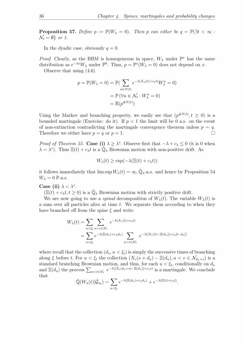
Recall from (4.3) thatWλ(t) =

∑u∈N(t)

e−λ(Xu(t)+cλt)

with cλ = λ/2 +mβ/λ = λ/2 + 1/λ is an additive martingale and that under Qλ thespine follows a Brownian motion with drift −λ (since the corresponding G martingaleis ζ(t) = e−λξ(t)−λ

2t/2). Let us define λ∗ :=√

2βm =√

2. Observe that λ 7→ cλ attainsits maximum on (−∞, 0) at −λ∗ and its minimum on (0,∞) at λ∗.

Theorem 55. The limit Wλ := limt→∞Wλ(t) exists P-almost surely and

4.6 Additive martingale convergence 35

Figure 4.1: The function λ 7→ cλ

(i) If |λ| ≥ λ∗ then W (λ) = 0 P-almost surely.

(ii) If |λ| ∈ [0, λ∗) then W (λ) is a L1(P) limit and P(Wλ > 0) = 1.

Remark 56. When the BBM is not dyadic one must further distinguish betweenthe cases E[A log+A] = ∞ (in which case Wλ(∞) = 0 even if |λ| < λ∗ ) andE[A log+A] <∞ (then it’s like in the dyadic case).

Before proving this Theorem we first give a decomposition and a 0-1 law result.Observe that

Wλ(t+ s) =∑u∈N(t)

∑u≤v∈N(t+s)

e−λ(Xv(t+s)+cλ(t+s))

=∑u∈N(t)

e−λ(Xu(t)+cλt)∑

u≤v∈N(t+s)

e−λ((Xv(t+s)−Xu(t))+cλs)

=∑u∈N(t)

e−λ(Xu(t)+cλt)W uλ (s)

where the W uλ (s) are i.i.d. copies of Wλ(s). By taking s→∞ we get

Wλ =∑u∈N(t)

e−λ(Xu(t)+cλt)W uλ (4.6)

where the W uλ are i.i.d. copies of Wλ started from one particle at the origin.

36 Chapter 4. Spines, martingales and probability changes

Proposition 57. Define p := P(Wλ = 0). Then p can either be q = P(∃t < ∞ :Nt = ∅ or 1.

In the dyadic case, obviously q = 0.

Proof. Clearly, as the BBM is homogeneous in space, Wλ under Px has the samedistribution as e−λxWλ under P0. Thus, p = Px(Wλ = 0) does not depend on x.Observe that using (4.6)

p = P(Wλ = 0) = P(∑u∈N(t)

e−λ(Xu(t)+cλt)W uλ = 0)

= P (∀u ∈ Nt : W uλ = 0)

= E(p#N(t))

Using the Markov and branching property, we easily see that (p#N(t), t ≥ 0) is abounded martingale (Exercise: do it). If p < 1 the limit will be 0 a.s. on the eventof non-extinction contradicting the martingale convergence theorem unless p = q.Therefore we either have p = q or p = 1.

Proof of Theorem 55. Case (i) λ ≥ λ∗. Observe first that −λ+ cλ ≤ 0 (it is 0 whenλ = λ∗). Thus Ξ(t) + cλt is a Qλ Brownian motion with non-positive drift. As

Wλ(t) ≥ exp(−λ(Ξ(t) + cλt))

it follows immediately that lim supWλ(t) =∞, Qλ-a.s. and hence by Proposition 54Wλ = 0 P-a.s.

Case (ii) λ < λ∗.(Ξ(t) + cλt, t ≥ 0) is a Qλ Brownian motion with strictly positive drift.We are now going to use a spinal decomposition of Wλ(t). The variable Wλ(t) is

a sum over all particles alive at time t. We separate them according to when theyhave branched off from the spine ξ and write

Wλ(t) =∑u<ξt

∑u<v∈Nt

e−λ(Xv(t)+cλt)

=∑u<ξt

e−λ(Ξ(du)+cλdu)∑

u<v∈Nt

e−λ([Xv(t)−Ξ(du)]+cλ[t−du])

where recall that the collection (du, u < ξt) is simply the successive times of branchingalong ξ before t. For u < ξt the collection (Xv(s + du) − Ξ(du), u < v ∈ Ndu+s) is astandard branching Brownian motion, and thus, for each u < ξt, conditionally on duand Ξ(du) the process

∑u<v∈Nt e

−λ([Xv(du+s)−Ξ(du)]+cλs) is a martingale. We concludethat

Q(Wλ(t)|G∞) =∑u<ξt

e−λ(Ξ(du)+cλdu) + e−λ(Ξ(t)+cλt).

4.7 First application : The speed of the rightmost particle 37

Using Fatou’s Lemma and the strong law of large numbers

Q(lim inft

Wλ(t)|G) ≤ lim sup Q(Wλ(t)|G)

≤ lim sup∑u<ξt

e−λ(ξdu+cλdu) + lim sup e−λ(ξt+cλt)

<∞ Qλ − a.s.

where we have used that there exists k > 0 such that Qλ-almost surely, for t largeenough λ(ξt + cλt) > kt.

Hence lim inf Wλ < ∞ Qλ-a.s. and thus Qλ-a.s. In a moment we will show that1/Wλ(t) is a Qλ-martingale (in the present case it actually is a martingale). As it’spositive it converges Qλ almost surely to its lim inf. By the dichotomy we now knowthat EP[Wλ(∞)] = 1 so that P(Wλ(∞) = 0) = 0.

To conclude, let us just show that 1/Wλ(t) is a Qλ-martingale. Suppose A ∈ Ft.Then

Q[1AWλ(t)

P(Wλ(t+ s) > 0|Ft)] = P[1AWλ(t)

P(Wλ(t+ s) > 0|Ft) ·Wλ(t)]

= P(A ∩ Wλ(t+ s) > 0)

= Q[1

Wλ(t+ s)1A].

4.7 First application : The speed of the rightmostparticle

Recall that λ∗ =√

2βm and let c∗ := cλ∗ = λ∗.

Theorem 58. Suppose A ≡ 1. The extremal particle has asymptotic speed√

2β, i.e.if we define M(t) := supu∈N(t) Xu(t)

M(t)

t→√

2β, P-a.s.

and furthermoreM(t)− c∗t→ −∞.

Proof. We use the additive martingale convergence Theorem 55. All the martingales

Wλ(t) =∑u∈N(t)

e−λ(Xu(t)+cλt)

38 Chapter 4. Spines, martingales and probability changes

converge. Furthermore,Wλ(t)→ 0 P-a.s. as soon as |λ| ≥ λ∗. Note that eλ∗(M(t)+c−λ∗ t) ≤W−λ∗(t) → 0 as soon as |λ| ≥ λ∗. Thus M(t) + c−λ∗t → −∞ and we just need toobserve that c−λ∗ = −c∗ to conclude that

M(t)− c∗t→ −∞.

and furthermore lim sup M(t)t≤ c∗.

We just need to prove the converse bound to conclude. When λ ∈ (−λ∗, 0], theprobabilities Qλ and P are equivalent. But since under Qλ the process Ξ(t) is a BMwith drift −λ we see that lim inf M(t)/t ≥ |λ|,Qλ-a.s. and thus P-a.s. as well. As λis arbitrary in (−λ∗, 0] we obtain lim inf M(t)/t ≥ λ∗,P-a.s.

Chapter 5Traveling waves

A striking feature of the KPP equation is that it is one of the simplest example of apartial differential equation which admits a traveling wave solution, that is

ut =1

2uxx + u(u− 1) (5.1)

has solutions of the form u(t, x) = w(x− ct). If such a solution exists it means thatu(x, t) is always a translate of the function w which we can thus see as a front withconstant shape moving with the velocity c on the real line.

Proposition 59. Let w : R→ [0, 1] be C2. Then u(t, x) = w(x− ct) is a solution of(5.1) if and only if

0 =1

2w′′ + cw′ + w(w − 1). (5.2)

One of the most striking result in Kolmogorov et al. original 1937 paper is thefollowing:

Theorem 60. Equation (5.1) has a monotone traveling wave wc of speed c if andonly if |c| ≥

√2. Furthermore, the traveling wave solution of speed c is unique up to

a shift in its argument and if c > 0 (resp. c < 0) it is increasing (resp. decreasing)with wc(−∞) = 0, wc(∞) = 1 (resp. wc(−∞) = 1, wc(∞) = 0).

The traveling wave with speed√

2, w = w√2 is often called the critical travelingwave. Remember that we also know from KPP, Bramson that

Theorem 61. If u is solution of (5.1) with initial condition u(0, x) = 1x≥0, thenu(t, x+mt)→ w(x) uniformly in x as t→∞

If we admit this, the results of Chapter 3 shows that

w(x) = E[

exp(− cZe−

√2x)]

and1− w(x) ∼ cxe−

√2x.

39

40 Chapter 5. Traveling waves

5.1 Traveling waves and multiplicative martingales

We now give a similar result for product martingales of the form

M(t) =∏

u∈N(t)

φ(Xu(t) + ct), t ≥ 0

where φ is a C2 map R 7→ [0, 1].

Proposition 62. Let φ : R 7→ R be a C2 function. It forms a product (local)martingale with (speed) parameter c,

Mφ(t) =∏

u∈N(t)

φ(Xu(t) + ct), t ≥ 0

if and only if φ solves (2.5)

1

2φ′′ + cφ′ + β(f(φ)− φ) = 0.

If in addition φ takes its values in [0, 1] then Mφ is a true martingale.

Proof of Proposition 62. Write F (t,X(t)) = Mφ(t) =∏

u∈N(t) φ(Xu(t) + ct). It iseasily seen that if φ solves (2.5) then

(G + ∂

∂t

)F ≡ 0 and thus by Proposition 12

(Mφ(t), t ≥ 0) is a local martingale.

Suppose now that there exists y such that 12φ′′(y) + cφ′(y) + β(f(φ) − φ)(y) > 0.

Then this implies that for t ≥ 0, x ∈ R such that x+ ct = y(G +

∂

∂t

)F (t, x) =

1

2φ′′(y) + cφ′(y) + β(f(φ)− φ)(y) > 0.

This would imply that

limε→0

E[F (t+ ε,X(t+ ε))|X(t) = x]− F (t, x)

ε> 0

which means that F (t,X(t)) cannot be a (local) martingale since For any Borel setA ⊆ R we have P(t,X(t) ∈ A) > 0.For instance, suppose that 1

2φ′′(y) + cφ′(y) + β(f(φ)− φ)(y) = η > 0 and define a

stopping time τ as follows:

τ = inft > 0 : #N(t) > 2 ∧ inft > 0 : (G + ∂t)F (t,X(t)) < η/2.

Now under Py, τ > 0 and E(τ) > 0 (properties of BM and continuity of φ, φ′ andφ′′). Thus

Ey(F (τ,X(τ))− F (0, y) = E(∫ τ

0

(G + ∂t)F (t,X(t)) dt

)> Ey(τ)η/2 > 0.

5.2 Existence of traveling waves at supercriticality 41

5.2 Existence of traveling waves at supercriticality

Definition 63. For λ ∈ R we define

Mλ(t) := E[e−Wλ(∞)|Ft

], t ≥ 0. (5.3)

The process (Mλ(t), t ≥ 0) is a martingale, bounded in [0, 1] and thus unifomlyintegrable with Mλ(t)→Mλ(∞) := e−Wλ(∞) almost surely and in L1. Define

wλ(x) := Ex[e−Wλ(∞)

]= E0

[e−e

−λxWλ(∞)],

and observe that when λ > 0, x 7→ wλ(x) is monotone and increases from 0 to 1(when Wλ(∞) is almost surely finite and not almost surely 0 when |λ| < λ∗, whichmeans |cλ| > c∗).Remember that we have he following decomposition

Wλ(∞) =∑u∈N(t)

e−λ(Xu(t)+cλt)W(u)λ (∞)

where the variables (W(u)λ (∞), u ∈ N(t)) are iid, independent of N(t) and distributed

as Wλ(∞). Thus

Mλ(t) = E[e−Wλ(∞)|Ft

]= E

∏u∈N(t)

e−e−λ(Xu(t)+cλt)W

(u)λ (∞)|Ft

=∏

u∈N(t)

E[e−e

−λ(Xu(t)+cλt)W(u)λ (∞)|Ft

]=∏

u∈N(t)

wλ(Xu(t) + cλt)

is a product martingale with speed cλ. To sum up

Theorem 64 (Existence). When |c| > c∗ the mapping,

wλ(x) = Exe−Wλ(∞)

where λ is picked so that c = cλ is a monotone traveling wave solution of (2.5) withspeed c.

Note that wλ is increasing from 0 to 1 if c > 0 and decreasing from 1 to 0 otherwise.

42 Chapter 5. Traveling waves

5.3 Non-existence of traveling waves atsubcriticality

Take c < c∗. Remember that if L(t) = minu∈N(t) Xu(t), by symetry

limt→∞

L(t) + ct = −∞.

Suppose that φc is a non-trivial TW of speed c with φc ∈ [0, 1], φc(−∞) = 0 andφc(+∞) = 1. We know that

M(t) :=∏

u∈N(t)

φc(Xu(t) + ct)

is a product martingale. Since it is bounded it is UI and converges a.s. and in L1.But ∏

u∈N(t)

φc(Xu(t) + ct) ≤ φc(L(t) + ct)→ 0

which is a contradiction. Hence, no bounded traveling waves from 0 to 1 exists atthis speed.

Chapter 6Extremal point process: The delay method

6.1 The centered maximum can’t converge in anergodic sense

Recall that by Kolmogorov result we know that if

u(t, x) = P(M(t) ≤ x)

thenu(t, x+mt)→ w(x) uniformly in x as t→∞

where w is the unique (up to a shift in the argument) solution of

0 =1

2w′′ +

√2w′ + w(w − 1).

Furthermore, we have seen that there exists c such that

1− w(y) ∼ cye−√

2y as y →∞.

This means in particular that M(t) − mt converges in distribution. But does itconverge in an ergodic sense, i.e. is it true that for all x ∈ R

limt→∞

1

t

∫ t

0

1M(s)−ms≤x ds→ w(x) a.s.?

A simple argument shows that this cannot be the case. Start two independentbranching Brownian motions, one form 0 and one from x and note Mx(t) fro themaximum of the one started form x.Then, by invariance by translation

limt→∞

1

t

∫ t

0

1Mx(s)−ms≤x ds = limt→∞

1

t

∫ t

0

1M(s)−ms≤0 ds = w(0)a.s.

43

44 Chapter 6. Extremal point process: The delay method

But there is a strictly positive probability that before any branching event, the twoinitial particles meet and realize a successful coupling (after this meeting time thetwo process stays identical) which implies that there is a positive probability for

limt→∞

1

t

∫ t

0

1Mx(s)−ms≤x ds = limt→∞

1

t

∫ t

0

1M(s)−ms≤x ds

or w(x) = w(0), which is a contradiction.

6.2 Convergence of the derivative martingale andthe centered maximum

We now show the results that were announced earlier

Proposition 65 (Convergence of the derivative martingale). Recall that the deriva-tive martingale is the process

Z(t) :=∑u∈Nt

(√

2t−Xu(t))e√

2(Xu(t)−√

2t)

Then, almost surelyZ(t)→ Z > 0.

Proof. From the multiplicative martingale principle we know that

W x(t) :=∏u∈Nt

w(√

2t−Xu(t) + x)

is an Ft-martingale which is positive and bounded. It thus converges almost surelyand L1 to its limit

W x := limtW x(t) ∈ [0, 1]

and EW x = w(x). Since minu∈Nt√

2t − Xu(t) + x → +∞ almost surely, the largetime behavior of W x is related to the asymptotic of w (this is essentially the samecalculation we already did). As t→ ∞

logW x(t) =∑u∈Nt

logw(√

2t−Xu(t) + x)

∼∑u∈Nt

−c(√

2t−Xu(t) + x) exp(√

2Xu(t)− 2t−√

2x)

∼ −cZ(t)e−√

2x − cxW−√2(t)e−√

2x

Remember that we know that W−√2(t)→ 0 almost surely. Thus

limtZ(t) =

(− e−

√2x/c

)logW x

6.2 Convergence of the derivative martingale and the centered maximum 45

This proves thatw(x) = E

[exp

(− cZ(∞)e−

√2x)]

which we already knew and that

Z(t)→ Z(∞) > 0 a.s.

Now, suppose P (Z(∞) =∞) > 0, and choose x such that E[W x] > 1−P(Z(∞) =∞)/2. Then

1− P(Z(∞) =∞)/2 < E[W x] = E[W x1Wx>0] ≤ P(W x > 0) = 1− P(Z(∞) =∞)

which is a contradiction.And Z(∞) > 0 is almost the same: suppose P(Z(∞) = 0) > 0, and choose x

such that E[W x] < P(Z(∞) = 0)/2 (we can do this since E[W x] = w(x) → 0 asx→ −∞). Then

P(Z(∞) = 0)/2 > E[W x] ≥ E[W x1Wx=1] = P(W x = 1) = P(Z(∞) = 0)

Now that we know that the derivative martingale converges to a non-degeneratepositive limit we can state lalley and Sellke’s main result

Theorem 66 (Lalley and Sellke, 1987 [22]). There exists a constant c > 0 such thatfor each x ∈ R

lims→∞

limt→∞

P(M(t+ s)−mt+s ≤ x

∣∣Fs) = exp− cZe−

√2xa.s. (6.1)

Consequently, the critical traveling wave has representation

w(x) = E exp− cZe−

√2x

(6.2)

and in particular1− w(x) ∼ cxe−

√2x as x→∞.

One can use the same proof as in Section 3. For self-containedness we replicate ithere.

Proof. As noted, mt+s = mt +√

2s+ ot(1). So we can write

P(M(t+ s)−mt+s lex

∣∣Fs) =∏u∈Nt

u(t, x+mt+s −Xu(s))

where u(t, x) = P(M(t) ≤ x) is the solution of the KPP equation with Heavisideinitial data. Combining all this together

limt→∞

P(M(t+ s)−mt+s lex

∣∣Fs) =∏u∈Nt

w(x+√

2s−Xi(s)) = W x(s).

This yields the claimed result.

46 Chapter 6. Extremal point process: The delay method

6.3 Heuristic meaning of Lalley and Sellke’s result

What does this result mean. Observe that if you treat Z as a known, fixed quantity(which you asymptotically can by conditioning on Fs with s big enough), then wehave the representation

P(M(t)−mt ≤ x) ∼ e−cZe−√

2x

= exp− e−

√2(x−2−1/2 log(cZ))

which we can rewrite as

P(√

2(M(t)−mt)− log(cZ) ≤ x) ∼ e−e−x.

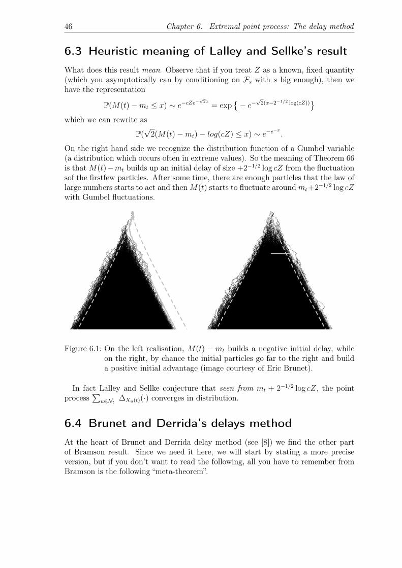
On the right hand side we recognize the distribution function of a Gumbel variable(a distribution which occurs often in extreme values). So the meaning of Theorem 66is that M(t)−mt builds up an initial delay of size +2−1/2 log cZ from the fluctuationsof the firstfew particles. After some time, there are enough particles that the law oflarge numbers starts to act and thenM(t) starts to fluctuate aroundmt+2−1/2 log cZwith Gumbel fluctuations.

Figure 6.1: On the left realisation, M(t) − mt builds a negative initial delay, whileon the right, by chance the initial particles go far to the right and builda positive initial advantage (image courtesy of Eric Brunet).

In fact Lalley and Sellke conjecture that seen from mt + 2−1/2 log cZ, the pointprocess

∑u∈Nt ∆Xu(t)(·) converges in distribution.

6.4 Brunet and Derrida’s delays method

At the heart of Brunet and Derrida delay method (see [8]) we find the other partof Bramson result. Since we need it here, we will start by stating a more preciseversion, but if you don’t want to read the following, all you have to remember fromBramson is the following “meta-theorem”.

6.4 Brunet and Derrida’s delays method 47

Theorem 67. If u solves

ut =1

2uxx + u(u− 1)

with initial condition u(0, x) = g(x) such that g = R→ [0, 1] with 1−g(x) = o(e−√

2x )then there exists a constant cg such that

u(t, x+mt)→ w(x+ cg)

where mt =√

2t− 32√

2log t and w is distribution function of the limit of M(t)−mt.

Let us now give a more precise statement. We consider the equation

ut =1

2uxx + f(u)

withf(0) = f(1) = 0, f(u) > 0 for 0 < u ≤ 1

andf ′(0) = 1, f ′(u) ≤ 1 for 0 < u ≤ 1

and we also assume that 1 − f ′(u) = O(uρ) for some ρ > 0. Also wc(x) denotes thetravelling wave with speed c >

√2. We set

c = cλ =1

λ+λ

2.

Theorem 68. Assume that the initial data is measurable with 0 ≤ u(0, x) ≤ 1 forall x. If c >

√2 then

u(t, x+m(t))→ wc(x)

uniformly in x as t → ∞ for some choice of m(t) if and only if for some (andequivalently, all) h > 0

limt→∞

1

tlog

[∫ t(1+h)

t

u(0, y)dy

]= −λ

and for some η > 0,M > 0 and N > 0∫ x+N

x

u(0, y)dy > η for x ≤ −M.

If c =√

2, thenu(t, x+m(t))→ w∗(x)

uniformly in x as t → ∞ for some choice of m(t) if and only if for some (andequivalently, all) h > 0

lim supt→∞

1

tlog

[∫ t(1+h)

t

u(0, y)dy

]= −√

2.

48 Chapter 6. Extremal point process: The delay method

The other very important result obtained by Bramson concerns the centering termm(t).

Theorem 69. Suppose that u(0, y) = Iy≤0 is the heavyside initial condition. Thenwe can chose

m(t) = 21/2t− 3.2−3/2 log t.

Define h(y) = u(0, y)e√

2y. If h(y) = yα for y ≥ 1 with α > −2 then we can chose

m(t) = 21/2t− (α− 1).2−3/2 log t

whereas when α ≤ −2m(t) = 21/2t− 3.2−3/2 log t

still holds.

Remark 70. 1. This means that if we define ma(t) = infx > 0 : u(t, x) = athen for any initial condition u0, x) = φ(x) that decays faster than e−21/2xx−2we have ma(t) = 21/2t− 3.2−3/2 log t+ δ(a, φ, f) where we call δ the delay.

2. Proof : Feynman-Kac integral with sample path estimates for Brownian motion.

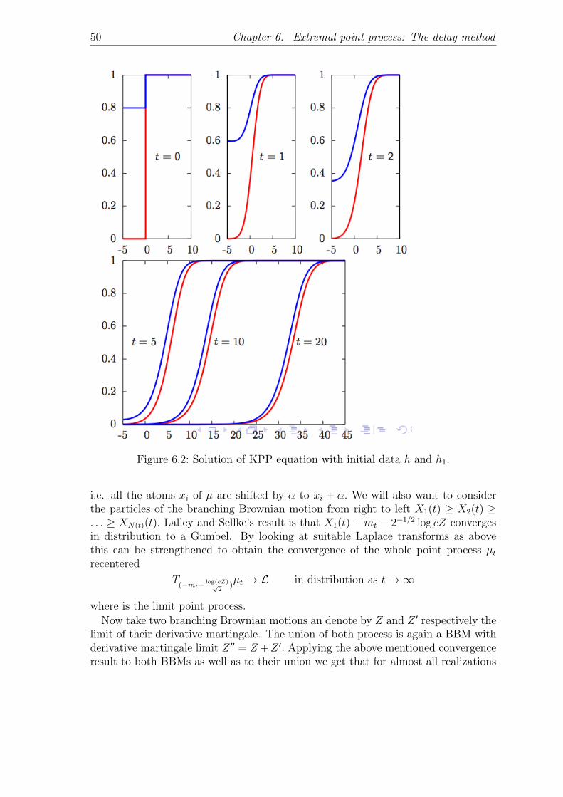
6.5 Laplace transforms

As we have seen, the initial data u(0, x) = h(x) = 1x≥0 leads (through McKean’srepresntation) to

u(t, x+mt) = Ex+mt [∏u∈Nt

h(Xu(t))]

= E0[∏u∈Nt

h(Xu(t) + x+mt)]

= E0[∏u∈Nt

h(x+mt −Xu(t))]

= E0[∏u∈Nt

1Xu(t)≤x+mt]

= P0(M(t) ≤ x+mt)→ w(x)

as t→∞ uniformly in x.Let us now employ a slightly different starting condition. For λ > 0 fixed, let

h1(x) = e−λ1x<0 + 1x≥0.

The same argument yields that

u(t, x+mt) = Ex+mt [∏u∈Nt

h1(Xu(t))]

= E0[∏u∈Nt

h1(x+mt −Xu(t))]

= E0[exp−λN[x,∞)(t)]

6.6 Superposability 49

where for A ⊂ RNA(t) = #u ∈ Nt : Xu(t)−mt ∈ A.

Thus, Bramson’s result for initial datum h1 reads

E0[exp−λN[x,∞)(t)]→ w(x+ ch1)

uniformly in x. This show that the variable N[x,∞)(t) converges in distribution ast→∞.For the convergence in distribution of the point process of particles centered by mt

µt(·) :=∑u∈Nt

δXu(t)−mt(·)

we need a bit more. We need that the joint-Laplace transforms of the number ofparticles in disjoint Borel sets converge. Fir λ, µ > 0 and x1 < x2 ∈ R consider

h2(x) :=

e−µx if x ≤ x1

e−λx if x ∈ [x1, x2]

1 if x > x2

Now, if u is the solution of KPP with h2 as initial datum, then the McKeanrepresentation tells us that

u(t,mt + x) = E0[e−µN[x−x1,∞)(t)e−λN[x−x2,x−x1) ]→ w(x+ ch2).

We can see that it is possible obtain in this way the convergence of the joint Laplacetransform of the number of particles in any finite collection of disjoint Borel setscentered around mt.We conclude that

Theorem 71 (Brunet and Derrida, 2011). The extremal point process centered bymt, i.e. µt(·) converges in distribution.

Remark 72. In fact, Brunet and Derrida show the convergence of the point processseen from M(t), the right-most particle.

6.6 Superposability

Now that we know that µt(·) converges in distribution, we want to know what thelimit looks like.Let us adopt a couple of notations. Given a point process µ(·) on R and α ∈ R we

define the shift operator Tα by

Tαµ(·) = µ(· − α)

50 Chapter 6. Extremal point process: The delay method

Figure 6.2: Solution of KPP equation with initial data h and h1.

i.e. all the atoms xi of µ are shifted by α to xi + α. We will also want to considerthe particles of the branching Brownian motion from right to left X1(t) ≥ X2(t) ≥. . . ≥ XN(t)(t). Lalley and Sellke’s result is that X1(t)−mt − 2−1/2 log cZ convergesin distribution to a Gumbel. By looking at suitable Laplace transforms as abovethis can be strengthened to obtain the convergence of the whole point process µtrecentered

T(−mt− log(cZ)√

2)µt → L in distribution as t→∞

where is the limit point process.Now take two branching Brownian motions an denote by Z and Z ′ respectively the

limit of their derivative martingale. The union of both process is again a BBM withderivative martingale limit Z ′′ = Z +Z ′. Applying the above mentioned convergenceresult to both BBMs as well as to their union we get that for almost all realizations

6.6 Superposability 51

of Z and Z ′, T log(c(Z+Z′))√2

L is equal in law to T log(cZ)√2

L + T2

log(cZ′)√2

L′ where L and L′

are two independent copies of the limit point process L. For simplicity let us forgetabout the factors 2−1/2 and c to obtain

L =dist Tlog(

ZZ+Z′

)L+ Tlog(

Z′Z+Z′

)L′Since Z and Z ′ can take any values (by varying the starting points of the BBMs forinstance) we see that for any a and b such that ea + eb = 1 we have

L =dist TaL+ TbL′

where L and L′ are two independent copies of L. Point processes with this propertyare called superposable by Brunet and Derrida or exponentially 1-stable by Maillard.What kind of point processes have this property?

Exercise 73. 1. Show that Poisson point processes with intensity e−x dx are su-perposable.

2. Let (Di) be a sequence of i.i.d. copies of a point process D, and let (xi)i∈N bethe atoms of a point process with intensity e−x dx. Show that

L =∑i

Tξi Di (6.3)

is superposable.

Brunet and Derrida asked if every superposable point process is in fact a decoratedexponential point process of the form (6.3). Maillard was able to show that this isindeed the case

Theorem 74. Every exponentially 1-stable point process is of the form (6.3) forsome decoration measure D.

It turns out that in addition to the simple proof of Maillard, this result can alsobe obtained from a classic result known as LePage decomposition of a stable pointprocess.

Chapter 7The extremal point process of thebranching Brownian motion

The study of the extremal point process of branching Brownian motion has been avery active area of research recently. In particular a full convergence result whichinclude the description of the decoration measure has been obtained independentlyby Arguin, Bovier and Kistler [3, 4, 5] on the one hand, and by Aïdekon, Berestycki,Brunet and Shi [2] on the other. The same type of result was obtained by Madaulefor branching random walks. One reason this type of results is interesting is thatit was conjectured, and indeed it has been confirmed to a large exttent, that theextrema of the Gaussian free field behave very much as the extrema of the branchingbrownian motions.

7.1 The setup

It is convenient when describing the extremal point process to get rid of the√

2t inthe position of the rightmost particle simply by adding a drift to the movements ofthe particles that tilts the cone shape of a branching Brownian motion in a space-timeplane. Furthermore, instead of considering the rightmost particles, we are going tolook at the leftmost ones. The process being symmetrical, this is of course arbitrary.

More precisely, the system starts with a single particle at the origin which followsa Brownian motion with drift % and variance σ2 > 0. Branching is dyadic and occurat rate β > 0.We are going to abuse the notation N (t) in order to designate both the collection

of particles alive at time t and the point measure of the particle positions. CallN(t) = #N (t) the number of particles alive at time t and X1(t) ≤ X2(t) ≤ · · · ≤XN(t)(t) their positions enumerated from left to right.

We will work impose the followin conditions: for all t > 0,

E[ ∑i=1,...,N(t)

e−Xi(t)]

= 1, E[ ∑i=1,...,N(t)

Xi(t)e−Xi(t)

]= 0. (7.1)

53

54 Chapter 7. The extremal point process of the branching Brownian motion

In this context the many-to-one Lemma tells us that for any measurable function Fand each t > 0,

E[ ∑i=1,...,N(t)

F (Xi,t(s), s ∈ [0, t])]

= eβt E[F (σBs + %s, s ∈ [0, t])

],

where, for each i ∈ 1, . . . , N(t) we let Xi,t(s), s ∈ [0, t] be the position, at time s,of the ancestor of Xi(t) and B is a standard Brownian motion. Thus the equations(7.1) become % = β+ σ2

2and % = σ2. Hence the usual conditions amount to supposing

% = σ2 = 2β. In these notes we always assume β = 1, ρ = 2 and σ =√

2.

7.2 Bramson and Lalley-Sellke in the new setup

Since we have changed the model slightly, we should start by reformulating Bramson’sresult in this context.There exists a constant CB ∈ R and a real valued random variable W such that

X1(t)−mtlaw→ W, t→∞, (7.2)

where

mt :=3

2log t+ CB (7.3)

and furthermore the distribution function of W is a solution to the critical Fisher-KPP travelling wave equation.The derivative martingale becomes simply

Z(t) :=∑

i=1,...,N(t)

Xi(t)e−Xi(t). (7.4)

and we have seen thatZ := lim

t→∞Z(t) (7.5)

exists and is strictly positive, finite with probability 1. The main result of Lalley’sand Sellke’s paper is then that ∃C > 0 such that

lims→∞

limt→∞

P(X1(t+ s)−m(t+ s) ≥ x|Fs) = exp (−CZex)

where Ft is the natural filtration of the branching Brownian motion. As a conse-quence,

P(W ≤ x) ∼ C |x|ex, x→ −∞. (7.6)

7.3 Main results 55

7.3 Main results

We consider the point process of the particles seen from the Lalley and Sellke refer-ential and enumerated from the leftmost:

¯N (t) := N (t)−mt + log(CZ) =Xi(t)−mt + log(CZ), 1 ≤ i ≤ N(t)

.

Theorem 75. As t → ∞ the pair ¯N (t), Z(t) converges jointly in distribution toL , Z where L and Z are independent and L is obtained as follows.

(i) Define P a Poisson point process on R, with intensity measure ex dx.

(ii) For each atom x of P, we attach a point process x + Q(x) where Q(x) areindependent copies of a certain point process Q.

(iii) L is then the superposition of all the point processes x + Q(x), i.e., L :=x+ y : x ∈P, y ∈ Q(x).

Exercise 76. Show that one can deduce from the above Theorem the following resultswhich concern the point process of positions seen from the leftmost particle

N ′(t) :=Xi(t)−X1(t), 1 ≤ i ≤ N(t)

.

As t→∞ the point process N ′(t) converges in distribution to the point process L ′

obtained by replacing the Poisson point process P in step (i) above by P ′ describedin step (i)’ below:

(i)’ Let e be a standard exponential random variable. Conditionally on e, defineP ′ to be a Poisson point process on R+, with intensity measure eex1R+(x) dxto which we add an atom in 0.

The decoration point process Q(x) remains the same.

We next give a precise description of the decoration point process Q which can beconsidered to be the main result of [2] (note that [5] give their own, quite differentdescription of the decoration). For each s ≤ t, let X1,t(s) be the position at time s ofthe ancestor of X1(t), i.e., s 7→ X1,t(s) is the path followed by the leftmost particleat time t. We define

Yt(s) := X1,t(t− s)−X1(t), s ∈ [0, t]

the time reversed path back from the final position X1(t). For each t > 0 and foreach path X := (X(s), s ∈ [0, t]) that goes from the ancestor to a particle in N (t),let us write (τXi ) for the successive splitting times of branching along the trajectoryX (enumerated backward), N (i)

t,X for the set of all particles at time t which aredescended from the one particle which has branched off X at time τXi relative to the

56 Chapter 7. The extremal point process of the branching Brownian motion

X1,t(t− s)

τ2(t)

τ3(t)

τ1(t)

N2(t)N1(t) N3(t)t

X1(t)X1,t(t)− b

Figure 7.1: (Y,Q) is the limit of the path s 7→ X1,t(t− s)−X1(t) and of the pointsthat have branched recently off from X1,t.

final position X(t) (see figure 7.3). More precisely, if we define τX,j(t) to be the timeat which the particle Xj(t) has branched off the path of X during [0, t] we have

N (i)t,X := Xj(t)−X(t), τX,j(t) = τXi .

We then defineQ(t, ζ) :=

⋃τX1(t)i >t−ζ

N (i)t,X1(t)

i.e., the set of particles at time t which have branched off X1,t(s) after time t− ζ.We will first show that (Yt(s), s ∈ [0, t]); Q(t, ζ) converges jointly in distribution

(by first letting t→∞ and then ζ →∞) towards a limit (Y (s), s ≥ 0); Q where thesecond coordinate is our point process Q which is described by growing conditionedbranching Brownian motions born at a certain rate on the path Y. We first describethe limit (Y (s), s ≥ 0),Q and then we state the precise convergence result.

The following family of processes indexed by a real parameter b > 0 plays a keyrole in this description. Let B := (Bt, t ≥ 0) be a standard Brownian motion andlet R := (Rt, t ≥ 0) be a three-dimensional Bessel process started from R0 := 0 andindependent from B. Let us define Tb := inft ≥ 0 : Bt = b. For each b > 0, wedefine the process Γ(b) as follows:

Γ(b)s :=

Bs, if s ∈ [0, Tb],

b−Rs−Tb , if s ≥ Tb.(7.7)

Let us defineGt(x) := P0(X1(t) ≤ x) = P−x(X1(t) ≤ 0)

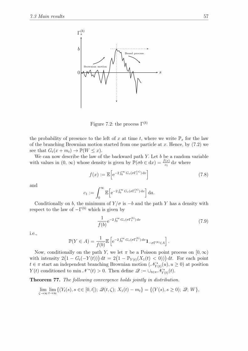
7.3 Main results 57

Brownian motion

Bessel process

0

b

s

!(b)s

1

Figure 7.2: the process Γ(b)

the probability of presence to the left of x at time t, where we write Px for the lawof the branching Brownian motion started from one particle at x. Hence, by (7.2) wesee that Gt(x+mt)→ P(W ≤ x).We can now describe the law of the backward path Y. Let b be a random variable

with values in (0, ∞) whose density is given by P(σb ∈ dx) = f(x)c1

dx where

f(x) := E[e−2

∫∞0 Gv(σΓ

(x)v ) dv

](7.8)

andc1 :=

∫ ∞0

E[e−2

∫∞0 Gv(σΓ

(a)v ) dv

]da.

Conditionally on b, the minimum of Y/σ is −b and the path Y has a density withrespect to the law of −Γ(b) which is given by

1

f(b)e−2

∫∞0 Gv(σΓ

(b)v ) dv (7.9)

i.e.,

P(Y ∈ A) =1

f(b)E[e−2

∫∞0 Gv(σΓ

(b)v ) dv1−σΓ(b)∈A

].

Now, conditionally on the path Y, we let π be a Poisson point process on [0,∞)with intensity 2

(1 − Gt(−Y (t))

)dt = 2

(1 − PY (t)(X1(t) < 0))

)dt. For each point

t ∈ π start an independent branching Brownian motion (N ∗Y (t)(u), u ≥ 0) at position

Y (t) conditioned to min N ∗(t) > 0. Then define Q := ∪t∈πN ∗Y (t)(t).

Theorem 77. The following convergence holds jointly in distribution.

limζ→∞

limt→∞(Yt(s), s ∈∈ [0, t]); Q(t, ζ); X1(t)−mt = (Y (s), s ≥ 0); Q; W,

58 Chapter 7. The extremal point process of the branching Brownian motion

where the random variable W is independent of the pair ((Y (s), s ≥ 0), Q), and Qis the point process which appears in Theorem 75.

Observe that the parameter ζ only matters for the decoration point process in thesecond coordinate.

7.4 A Laplace transform result

Using the less trivial version of the many-to-one result yields a first result whichturns out to be an important element in the proofs.Theorem 78 characterizes the joint distribution of the path s 7→ X1,t(s) that the

particle which is the leftmost at time t has followed, of the point processes of theparticles to its right and the times at which these particles have split in the past interms of a Brownian motion functional.For any positive measurable functional F and any positive measurable function

f : [0, t] → R+, for n ∈ N, (α1, . . . , αn) ∈ Rn+ and A1, . . . , An a collection of Borel

subsets of R+ define

I(t) := EF (X1,t(s), s ∈ [0, t]) exp

(−∑i

f(t−τX1,t

i )n∑j=1

αj#[N (i)t,X1(t)∩(X1(t)+Aj)]

),

For each r ≥ 0 and every x ∈ R recall that Gr(x) = PX1(r) ≤ x, and furtherdefine

G(f)

r (x) := E[e−f(r)

∑nj=1 αj#[N (r)∩(x+Aj)] 1X1(r)≥x

].

Hence, when f ≡ 0 we have G(f)

r (x) = 1−Gr(x).

Theorem 78. We have

I(t) = E[eσBt F (σBs, s ∈ [0, t]) e−2

∫ t0 [1−G(f)

t−s(σBt−σBs)] ds], (7.10)

where B in the expectation above is a standard Brownian motion. In particular, thepath (s 7→ X1,t(s), 0 ≤ s ≤ t) is a standard Brownian motion in a potential:

E[F (X1,t(s), s ∈ [0, t])

]= E

[eσBt F (σBs, s ∈ [0, t]) e−2

∫ t0 Gt−s(σBt−σBs) ds

]. (7.11)

The proof relies on the use of the following version of the many-to-one principle.We are going to use the critical additive martingale (which converges to zero) Theprocess

Mt :=∑i≤N(t)

e−Xi(t), t ≥ 0.

7.4 A Laplace transform result 59

Let Q be the probability measure on F∞ such that, for each t ≥ 0,

Q|Ft= Mt • P|Ft

.

Under Q the particle with label ξs at time s branches at (accelerated) rate 2 andgives birth to normal branching Brownian motions (without spine) with distributionP, whereas the process of the position of the spine (Ξ(s), s ∈ [0, t]) is a driftlessBrownian motion of variance σ2 = 2. Furthermore, for each t ≥ 0 and each i ≤ N(t),

QΞt = i |Ft =e−Xi(t)

Mt

.

For each i ≤ N(t) consider Ψi a random variable which is measurable in the filtra-tion of the branching Brownian motion up to time t (i.e., it is determined by the his-tory of the process up to time t) and suppose that we wish to compute EP[

∑i≤N(t) Ψi].

Then, thanks to the above, we have

EP

[ ∑i≤N(t)

Ψi

]= EQ

[ 1

Mt

∑i≤N(t)

Ψi

]= EQ

[eΞ(t)Ψξt

]. (7.12)

Proof. For the sake of brevity let us only treat the case where f ≡ 0. Letting Xi,t(s)be the position of the ancestor at time s of the particle at Xi(t) at time t, we have

I(t) = E[ ∑i≤N(t)

1i=1 F (Xi,t(s), s ∈ [0, t])],

Using the many-to-one principle and the change of probability presented in equation(7.12) we see that

I(t) = EQ

[eΞ(t) 1Ξt=1 F (Ξ(s), s ∈ [0, t])

]= EQ

[eΞ(t) F (Ξ(s), s ∈ [0, t])

∏k

1min N(ξt)k >0

]where we recall that by convention, for a point measure N , min N is the infimumof the support of N .Conditioning on the σ-algebra generated by the spine (including the successive

branching times) we obtain

I(t) = EQ

[eΞ(t) F (Ξ(s), s ∈ [0, t])

∏i

(1−G(f)

t−τ (ξt)i (t)

(Ξ(t)− Ξ(τ(ξt)i (t)))

)],

where, recall that for any r ≥ 0 and any x ∈ R,

G(f)r (x) := E

[1min N (r)≤x

]. (7.13)

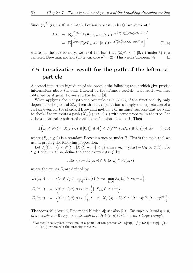
60 Chapter 7. The extremal point process of the branching Brownian motion

Since (τ(Ξt)i (t), i ≥ 0) is a rate 2 Poisson process under Q, we arrive at:1

I(t) = EQ

[eΞ(t) F (Ξ(s), s ∈ [0, t]) e−2

∫ t0 [G

(f)t−s(Ξ(t)−Ξ(s))] ds

]= E

[eσBt F (σBs, s ∈ [0, t]) e−2

∫ t0 [G

(f)t−s(σBt−σBs)] ds

], (7.14)

where, in the last identity, we used the fact that (Ξ(s), s ∈ [0, t]) under Q is acentered Brownian motion (with variance σ2 = 2). This yields Theorem 78.

7.5 Localization result for the path of the leftmostparticle

A second important ingredient of the proof is the following result which give preciseinformations about the path followed by the leftmost particle. This result was firstobtained by Arguin, Bovier and Kistler in [3].When applying the many-to-one principle as in (7.12), if the functional Ψξ only

depends on the path of Ξ(s) then the last expectation is simply the expectation of acertain event for the standard Brownian motion. For instance, suppose that we wantto check if there exists a path (Xi,t(s), s ∈ [0, t]) with some property in the tree. LetA be a measurable subset of continuous functions [0, t] 7→ R. Then

P(∃i ≤ N(t) : (Xi,t(s), s ∈ [0, t]) ∈ A

)≤ P(eσBt ; (σBs, s ∈ [0, t]) ∈ A) (7.15)

where (Bs, s ≥ 0) is a standard Brownian motion under P. This is the main tool weuse in proving the following proposition.Let Jη(t) := i ≤ N(t) : |Xi(t) −mt| < η where mt = 3

2log t + CB by (7.3). For

t ≥ 1 and x > 0, we define the good event At(x, η) by

At(x, η) := E1(x, η) ∩ E2(x, η) ∩ E3(x, η)

where the events Ei are defined by

E1(x, η) :=∀i ∈ Jη(t), min

[0,t]Xi,t(s) ≥ −x, min

[ t2, t]Xi,t(s) ≥ mt − x

,

E2(x, η) :=∀i ∈ Jη(t),∀s ∈ [x,

t

2], Xi,t(s) ≥ s1/3

,

E3(x, η) :=∀i ∈ Jη(t),∀s ∈ [

t

2, t− x], Xi,t(s)−Xi(t) ∈ [(t− s)1/3, (t− s)2/3]

.

Theorem 79 (Arguin, Bovier and Kistler [3]; see also [2]). For any ε > 0 and η > 0,there exists x > 0 large enough such that P(At(x, η)) ≥ 1− ε for t large enough.

1We recall the Laplace functional of a point Poisson process P: E[exp(−∫f dP)] = exp[−

∫(1−

e−f ) dµ], where µ is the intensity measure.

7.5 Localization result for the path of the leftmost particle 61

mtmt − x

t− x

X1(t)

X1(t) + (t− s)1/3

X1(t) + (t− s)2/3

t1/3

t/2

t/2 t

0−x

0

t

x

Figure 7.3: The events E1(x, η), E2(x, η) and E3(x, η) together are the event that thepaths of particles ending within distance η of mt avoid all the dashedregions.

The proof of this result is quite involved. Essentially one starts by showing thatfor x large enough P(E1(x, η)) < ε (where ε, η are given). Then, conditionally onE1(x, η)one shows that P(E2(x, η)) < ε, and so on.To give a taste of the technicalities involved here let us just focus on the proof of

the bound of P(E2(x, η)).

Proof. We can restrict to the event E1(z, η) for z large enough. By the many-to-oneprinciple, we get

P(E2(x, η), E1(z, η)) ≤ eη+CB t3/2P(B)

where P(B) is defined by

P(B) := P∃s ∈ [x, t/2] : σBs ≤ s1/3, σB[0,t/2] ≥ −z, σB[t/2,t] ≥ mt−z, σBt ≤ mt+η

.

We will actually bound the probability

P(B, dr) (7.16)

:= P∃s ∈ [x, t/2] : σBs ≤ s1/3, σB[0,t/2] ≥ −z, σB[t/2,t] ≥ mt − z, σBt ∈ mt + dr

.

Applying the Markov property at time t/2 yields that

P(B, dr)

= E[1∃s∈[x,t/2]:σBs≤s1/31σB[0,t/2]≥−zPBt/2

σB[0,t/2] ≥ mt − z, σBt/2 ∈ mt + dr

]≤ c(r + z)t−3/2E

[1∃s∈[x,t/2]:σBs≤s1/31σB[0,t/2]≥−z(σBt/2 −mt + z)+

]dr

≤ c(r + z)t−3/2E[1∃s∈[x,t/2]:σBs≤s1/31σB[0,t/2]≥−z(σBt/2 + z)

]dr

62 Chapter 7. The extremal point process of the branching Brownian motion

where the second inequality comes from the joint law of a Brownian motion and itsinfimum), and we set y+ := max(y, 0). We recognize the h-transform of the Besselprocess. Therefore

P(B, dr) ≤ cz(r + z)t−3/2Pz(∃s ∈ [x, t/2] : σRs ≤ z + s1/3) dr (7.17)

where as before (Rs, s ≥ 0) is a three-dimensional Bessel process. In particular,P(B) =

∫ η−z P(B, dr) ≤ cz(z + η)2t−3/2Pz(∃s ∈ [x, t/2] : σRs ≤ z + s1/3). This yields

that

P(E2(x, η), E1(z)) ≤ eη+CBcz(z + η)2Pz(∃s ∈ [x, t/2] : σRs ≤ z + s1/3)

≤ eη+CBcz(z + η)2Pz(∃s ≥ x : σRs ≤ z + s1/3)

and we deduce that P(E2(x, η), E1(z)) ≤ ε for x large enough.

7.6 The point process of the clan-leaders

We are now going to explain the structure of the limit point process as a decoratedPoisson point process as follows. We show that by stopping particles when they firsthit a certain position k and then considering only their leftmost descendants onerecovers a Poisson point measure of intensity ex dx as k → ∞. Then, we show thattwo particles near mt have separated in a branching event that was either very recentor near the very beginning of the process and we finally combine those two steps tocomplete the proof of Theorem 75.We employ a very classical approach: we stop the particles when they reach an

increasing family of affine stopping lines and then consider their descendants inde-pendently. The same kind of argument with the same stopping lines appear in [21]and in [1].

Fix k ≥ 1 and consider Hk the set of all particles which are the first in their lineof descent to hit the spatial position k. (For the formalism of particle labelling, seeNeveu [27].) Under the conditions we work with, we know that almost surely Hk isa finite set. The set Hk is again a dissecting stopping line at which we can apply thethe strong Markov property (see e.g. [11]). We see that conditionally on FHk

— thesigma-algebra generated by the branching Brownian motion when the particles arestopped upon hitting the position k — the subtrees rooted at the points of Hk areindependent copies of the branching Brownian motion started at position k and atthe random time at which the particle considered has hit k. Define Hk := #Hk and

Zk := ke−kHk.

Neveu ([27], equation (5.4)) shows that the limit Z of the derivative martingale in(7.4) can also be obtained as a limit of Zk (it is the same martingale on a differentstopping line)

Z = limk→∞

Zk = limk→∞

ke−kHk (7.18)

7.6 The point process of the clan-leaders 63

almost surely. Let us further define Hk,t as the set of all particles which are the firstin their line of descent to hit the spatial position k, and which do so before time t.

For each u ∈ Hk,t, let us write Xu1 (t) for the minimal position at time t of the

particles which are descendants of u. If u ∈ Hk\Hk,t we define Xu1 (t) = 0. This

allows us to define the point measure

P∗k,t :=

∑u∈Hk

δXu1 (t)−mt+log(CZk).

We further defineP∗

k,∞ :=∑u∈Hk

δk+W (u)+log(CZk)

where, conditionally on FHk, theW (u) are independent copies of the random variable

W in (7.2).

Proposition 80. The following convergences hold in distribution

limt→∞

P∗k,t = P∗

k,∞

andlimk→∞

(P∗k,∞, Zk) = (P, Z)

where P is as in Theorem 75, Z is as in (7.5), and P and Z are independent.

Proof. Fix k ≥ 1. Recall that Hk is the set of particles absorbed at level k, andHk = #Hk. Observe that for each u ∈ Hk, Xu

1 (t) has the same distribution ask + X1(t − ξk,u), where ξk,u is the random time at which u reaches k. By (7.2) andthe fact that mt+c −mt → 0 for any c, we have, for all k ≥ 1 and all u ∈Hk,

Xu1 (t)−mt

law→ k +W, t→∞.Hence, the finite point measure Pk,t :=

∑u∈Hk

δXu1 (t)−mt converges in distribution

as t → ∞, to Pk,∞ :=∑

u∈Hkδk+W (u), where conditionally on Hk, the W (u) are

independent copies of W . This proves the first part of Proposition 80.

The proof of the second part relies on some classical extreme value theory. Werefer the reader to [29] for a thorough treatment of this subject. Let us state theresult we will use. Suppose we are given a sequence (Xi, i ∈ N) of i.i.d. randomvariables such that

P(Xi ≥ x) ∼ Cxe−x, as x→∞.Call Mn = maxi=1,...,nXi the record of the Xi. Then it is not hard to see that if welet bn = log n+ log log n we have as n→∞

P(Mn − bn ≤ y) = (P(Xi ≤ y + bn))n

= (1− (1 + o(1))C(y + bn)e−(y+bn))n

∼ exp(− nC(y + bn)

1

n log ne−y)

∼ exp(−Ce−y)

64 Chapter 7. The extremal point process of the branching Brownian motion

and therefore

P (Mn − bn − logC ≤ y) ∼ exp(−e−y).

By applying Corollary 4.19 in [29] we immediately see that the point measure

ζn :=n∑i=1

δXi−bn−logC

converges in distribution to a Poisson point measure on R with intensity e−x dx.This result applies immediately to the random variables −W (u) (recalling from

(7.6) that P(−W ≥ x) ∼ Cxe−x, x→∞) and thus the point measure∑u∈Hk

δW (u)+(logHk+log logHk+logC)

converges (as k → ∞) in distribution towards a Poisson point measure on R withintensity ex dx (it is ex instead of e−x because we are looking at the leftmost particles)independently of Z (this identity comes from (7.18)). By definition Hk = k−1ekZk,thus

logHk = k + logZk − log k

log logHk = log k + log(1 + ok(1))

where the term ok(1) tends to 0 almost surely when k →∞. Hence,

logHk + log logHk = logZk + k + ok(1).

We conclude that for u ∈Hk

k +W (u) + log(CZ) = W (u) + (logHk + log logHk + logC) + ok(1).

Hence we conclude that

P∗k,∞ =

∑u∈Hk

δk+W (u)+log(CZ)

also converges (as k → ∞) towards a Poisson point measure on R with intensityex dx independently of Z = limk Zk. This concludes the proof of Proposition 80.

7.7 Genealogy near the extrema

The following result shows that near the rightmost particle at time t, particles haveeither a very recent common ancestor, or they have branched a very long time ago.Recall that Jη(t) := i ≤ N(t) : |Xi(t) − mt| ≤ η is the set of indices which

correspond to particles near mt at time t and that τi,j(t) is the time at which theparticles Xi(t) and Xj(t) have branched from one another.

7.7 Genealogy near the extrema 65

Proposition 81. (Arguin, Bovier and Kistler [3]) Fix η > 0 and any function ζ :[0,∞)→ [0,∞) which increases to infinity. Define the event

Bη,k,t := ∃i, j ∈ Jη(t) : τi,j(t) ∈ [ζ(k), t− ζ(k)] .

One haslimk→∞

limt→∞

P [Bη,k,t] = 0. (7.19)

We only sketch the beginning of a spine proof of this result here.

Proof. Fix η > 0 and k → ζ(k) an increasing sequence going to infinity. We want tocontrol the probability of

Bη,k,t = ∃i, j ∈ Jη(t) : τi,j(t) ∈ [ζ(k), t− ζ(k)]

the “bad" event that particles have branched at an intermediate time when t → ∞and then k →∞.By choosing x large enough, we have for all ζ ≥ 0 and t large enough

P(∃i, j ∈ Jη(t) : τi,j(t) ∈ [ζ, t− ζ])

≤ P(At(x, η)) + P(∃i, j ∈ Jη(t) : τi,j(t) ∈ [ζ, t− ζ], At(x, η))

≤ ε+ E

1At(x,η)

∑i∈Jη(t)

1∃j∈Jη(t):τi,j(t)∈[ζ,t−ζ]

.Using the many-to-one principle, we have

E

1At(x,η)

∑i∈Jη(t)

1∃j∈Jη(t):τi,j(t)∈[ζ,t−ζ]

= EQ

[eΞ(t)1At(x,η)1|Ξ(t)−mt|≤η,∃j∈Jη(t):τΞ,j(t)∈[ζ,t−ζ]

]where τΞ,j(t) is the time at which the particle Xj(t) has branched off the spine Ξ.In particular, using the description of the process under Q, we know that Ξ(t) isσ times a standard Brownian motion, and that independent branching Brownianmotions are born at rate 2 (at times (τ

(Ξt)i (t), i ≥ 1)) from the spine Ξ. The event

∃j ∈ Jη(t) : τΞ,j(t) ∈ [ζ, t − ζ] means that there is an instant τ (Ξt)i (t) between ζ

and t− ζ, such that the branching Brownian motion that separated from Ξ at thattime has a descendant at time t in [mt − η,mt + η]. In particular, the minimum ofthis branching Brownian motion at time t is lower than mt + η. Thus

EQ

[eΞ(t)1At(x,η)1|Ξ(t)−mt|≤η,∃j∈Jη(t):τΞ,j(t)∈[ζ,t−ζ]

]≤ EQ

[eΞ(t)1At(x,η)1|Ξ(t)−mt|≤η

∑τ∈[ζ,t−ζ]

1Xτ1,t≤mt+η

]where Xτ

1,t is the leftmost particle at time t descended from the particle whichbranched off Ξ at time τ , and the sum goes over all times τ = τ

(Ξt)i (t) ∈ [ζ, t − ζ]

66 Chapter 7. The extremal point process of the branching Brownian motion

at which a new particle is created. Recall that Gv(x) = P(X1(v) ≤ x) so that byconditioning we obtain

EQ

[eΞ(t)1At(x,η)1|Ξ(t)−mt|≤η,∃j∈Jη(t):τΞ,j(t)∈[ζ,t−ζ]

]≤ EQ

[eΞ(t)1At(x,η)1|Ξ(t)−mt|≤η

∑τ∈[ζ,t−ζ]

Gt−τ (mt + η −XΞτ (τ))].

The rest of the proof works roughly as follows: the event At(x, η) localizes thepath Ξ as explained above, which allows us to lower bound the path Ξ by s1/3 on[ζ, t/2] and by (t − s)1/3 on [t/2, t − ζ]. This in turn allows us to upper bound thelast expression.

7.8 The last piece

Recall that ∀u ∈Hk, Xu1 (t) is the position at time t of the leftmost descendent of u

(or 0 if u 6∈ Hk,t), and let Xu1,t(s), s ≤ t be the position at time s of the ancestor of

this leftmost descendent (or 0 if u 6∈Hk,t). For each t, ζ and u ∈Hk define

Q(u)t,ζ = δ0 +

∑i:τui >t−ζ

N ui

where the τui are the branching times along the path s 7→ Xu1,t(s) enumerated back-

ward from t and the N ui are the point measures of particles whose ancestor was born

at τui (this measure has no mass if u 6∈ Hk,t). Thus, Q(u)t,ζ is the point measure of

particles which have branched off the path s 7→ Xu1,t(s) at a time which is posterior

to t− ζ, including the particle at Xu1 (t).

In the same manner we define Qζ as the point measure obtained from Q (inTheorem 77) by only keeping the particles that have branched off s 7→ Y (s) beforeζ. More precisely, conditionally on the path Y, we let π be a Poisson point processon [0,∞) with intensity 2

(1 − Gt(−Y (t))

)dt = 2

(1 − PY (t)(X1(t) < 0))

)dt. For

each point t ∈ π such that t < ζ, start an independent branching Brownian motion(N ∗

Y (t)(u), u ≥ 0) at position Y (t) conditioned to have min N ∗Y (t)(t) > 0. Then define

Qζ := δ0 +∑

t∈π,t<ζ N ∗Y (t)(t).

Lemma 82. For each fixed k and ζ, the following limit holds in distribution

limt→∞

(P∗k,t, (Q

(u)t,ζ )u∈Hk

) = (P∗k,∞, (Q

(u)ζ )u∈Hk

)

where (Q(u)ζ )u∈Hk

is a collection of independent copies of Qζ, independent of P∗k,∞.

Proof. Conditionally on Hk, the random variables (Xu1,t(·), Q(u)

t,ζ )u∈Hkare indepen-

dent by the branching property. By Theorem 77, for every u ∈ Hk, the pair(Xu

1 (t) − mt, Q(u)t,ζ ) converges in law to (k + W (u), Q(u)

ζ ) where Q(u)ζ is a copy of

Qζ independent of W (u).

7.9 Putting the pieces back together: Proof of Theorem 75 67

To conclude, observe that∑

u∈Hkδk+W (u) = P∗

k,∞ − log(CZk) by Proposition 80.Since for each u ∈Hk the point measure Q(u)

ζ is independent ofW (u) and of allW (v)

for v ∈ Hk and v 6= u, it follows that Q(u)ζ is independent of P∗

k,∞. We concludethat

limt→∞

(P∗k,t, (Q

(u)t,ζ )u∈Hk

) = (P∗k,∞, (Q

(u)ζ )u∈Hk

)

in distribution where the two components of the limit are independent.

7.9 Putting the pieces back together: Proof ofTheorem 75

Let ¯N (k)(t) be the extremal point measure seen from the position mt − log(CZk)

¯N (k)(t) := N (t)−mt + log(CZk).

Let ζ : [0,∞)→ [0,∞) be any function increasing to infinity. Observe that on Bη,k,t

(an event of probability tending to one when t→∞ and then k →∞ by Proposition81) we have

¯N (k)(t)|[−η,η] =∑u∈Hk

(Q(u)t,ζ(k) +Xu

1,t −mt + log(CZk))|[−η,η)].

Now by Lemma 82 we know that in distribution

limt→∞

∑u∈Hk

(Q(u)t,ζ(k) +Xu

1,t −mt + log(CZk))

=∑

x∈P∗k,∞

(x+ Q(x)ζ(k))

where the Q(x)ζ(k) are independent copies of Qζ(k), and independent of Hk. Moreover,

we know that limt→∞ Z(t) = Z almost surely.By the second limit in Proposition 80, we have that (

∑x∈P∗k,∞

(x + Q(x)ζ(k)), Zk)

converges as k → ∞ to (L , Z) in distribution, L being independent of Z. Inparticular, (L , Z) is also the limit in distribution of (

∑x∈P∗k,∞

(x + Q(x)ζ(k)), Z). We

conclude that in distribution

limk→∞

limt→∞

( ¯N (k)(t)|[−η,η)], Z(t)) = (L |[−η,η)], Z).

Hence, limk→∞ limt→∞( ¯N (k)(t), Z(t)) = (L , Z) in distribution. Since ¯N (t) is ob-tained from ¯N (k)(t) by the shift log(CZ) − log(CZk), which goes to 0 by (7.18),we have in distribution limt→∞( ¯N (t), Z(t)) = (L , Z) which yields the content ofTheorem 75.

68 Chapter 7. The extremal point process of the branching Brownian motion

7.10 The approach and description of Arguin et al.

In [4], Arguin, Bovier and Kistler using the path localization argument obtainedin [3] are able to show that if one only considers particles that have branched offfrom one another far enough into the past (the point process of clan leaders), thenit converges to a Poisson point process with exponential intensity ([4], Theorem 2).Their proof relies on the convergence of Laplace functionals (for which a first Lalley-Sellke type representation is given) and not from the classical results about recordsof iid variables as here.

In [5] a complete description of the extremal point process of the branching Brow-nian motion is given. There, they show that ¯N (t) (actually in [5] the point processN is centered by mt instead of mt − log(CZ)) converges in distribution to a lim-iting point process which is necessarily an exponential Poisson point process whoseatoms are “decorated" with iid point measures. They give a complete descriptionof this decoration point measure as follows. Let D(t) =

∑∞i=1 δXi(t)−X1(t) which is a

random point measure on R+. Conditionally on the event X1(t) < 0 it converges indistribution to a limit D.One of the key argument in [5] is to identify the limit extremal point process of

the branching Brownian motion with the limit of an auxiliary point process. Thisauxiliary point process is constructed as follows. Let (ηi, i ∈ N) be the atoms of aPoisson point process on R+ with intensity

a(xebx) dx

for some constants a and b. For each i, they start form ηi an independent branchingBrownian motion (with the same λ, σ, % parameters as the original one) and call Π(t)the point process of the position of all the particles of all the branching Brownianmotions at time t. Theorem 2.5 in [5] shows that limt→∞Π(t) = limt→∞ ¯N (t). Thissolves what Lalley and Sellke [22] call the conjecture on the standing wave of particles.The proof is based on the analysis of Bramson [7] for the solution of the F-KPPequation with various initial conditions and the subsequent work of Lalley and Sellke[22] and Chauvin and Rouault [10] which allows them to show convergences of Laplacetype functionals of the extremal point process.

Chapter 8Branching Brownian motion withabsorption

In this chapter we are going to start our analysis of branching Brownian motion withabsorption. In its simplest instance, the definition of the model is straightforward.We start a usual branching Brownian motion with dirt µ ∈ R from a single particleat position x > 0 and we kill particles when they hit the origin.Such a model is clearly coupled with the usual branching Brownian motion as

follows. Let (X(t), t ≥ 0) be a usual Px-branching Brownian motion with drift µstarted from x and N (t) be the set of particles alive at time t for this full BBM.Define

Nabs(t) = u ∈ N (t) : infs≤t

Xu(s) > 0.

Then (Xu(t), u ∈ Nabs(t), t ≥ 0) is the branching Brownian motion with absorp-tion. We have just kept all the particles whose path has not touched 0.

Since the branching Brownian motion with or without absorption are thus definedon the same probability space, we use the same notation Px for their law, or sometimesPµ,x when we wish to emphasize the dependence on the drift parameter.

8.1 Survival and Kesten’s result

The first question we may ask about this process is wether it survives or not. Clearlythis will depend on the value of µ. Recall that under P0,0 when there is no drift, wehave shown that

M(t)

t→√

2, almost surely.

Therefore one can guess the following result which is first proved by kesten in 78 [?]:

Theorem 83. Let ζ := inft ≥ 0 : Nabs(t) = ∅ be the extinction time of the BBMwith absorption. Then, P(ζ <∞) = 1 if and only if µ ≤ −

√2.

69

70 Chapter 8. Branching Brownian motion with absorption

Proof. Observe that this is not a simple consequence of the almost sure limit ofM(t)/t which only implies that if µ ≤ −

√2 then P(ζ < ∞) = 1 (in fact for the

equality case we need to use that M(t)−√

2t→ −∞).So we only need to show that for µ > −

√2 there is a positive probability that the

process survives forever. Observe that this equivalent to asking that in a BBM withzero drift started form 0, there exists a particle u ∈ U such that

Xu(t) ≥ −µt− x,∀t ≥ 0

[insert figure]This can be done most efficiently through the use of the change of probability

Wλ(t). Indeed, choose λ ∈ (−√

2, µ) so that Qλ ∼ P. Under Qλ we know that Ξ is aBM with drift −λ and therefore

Qλ

(∀t ≥ 0 : Ξ(t) > −λt− x

)> 0

and thusP(∃u ∈ U s.t. ∀t ≥ 0 : Xu(t) > −λt− x

)> 0.

8.2 Refinement By Feng-Zeitouni and Jaffuel

8.3 The number of absorbed particles: regime A(Maillard’s result)

8.4 The number of absorbed particle: Regime C(the distribution of the all time minimum)

8.5 The number of absorbed particles: Regime B(convergence to the traveling wave

Chapter 9Populations under selection andBrunet-Derrida’s conjectures

In this chapter, I will try to describe a series of conjectures by Brunet and Derridaconcerning branching random walks -or branching Brownian motion- with sélection.I will then présent briefly some of the results we have obtained concerning theseconjectures in [?] and [?] as well as the beautiful results of Maillard [?].

9.1 Brunet-Derrida conjectures

9.1.1 BRW and BBM with selection

In [?, ?, ?] Brunet, Derrida, Mueler and Munier study various models of populationunder selection and use this to obtain results concerning the noisy FKPP equation.To fix things, let us consider the following two models.

Model 1: the BRW with selection We have a population of size N with asexualreproduction. Each individual i ≤ N is completely characterized by a number xi ∈ Rwhich measures its salective advantage and that we interpret as his fitness. So at agiven time the population is simple a collection of N points on the real line. Time isdiscrete and at each generation the whole population is entirely renewed accordingto the following two-steps mechanism

Reproduction-mutation : each individual has k offsprings (so that after thisstep there is momentarily kN particles) and the relative positions of offspringswith respect to their parents are given by i.i.d. copies of a certain displacementlaw ρ.

Selection : Just keep the N rightmost particles among the kN you have justcreated.

A good example to keep in mind is the case k = 2 and ρ the uniform distribution on[0, 1] (typically want second moments and no lattice).

71

72 Chapter 9. Populations under selection and Brunet-Derrida’s conjectures

Model 2: the BBM with selection We still have a cloud of N particles thatleaves on R. The evolution of the population is still essentially following the samesteps

Reproduction-mutation : each particle moves in R according to an inde-pendent Brownian motion and branches at rate 1 into two new particles whichthen start to follow the same behavior and so on. If we stop here, this is justthe standard branching Brownian motion.

Selection : At each branching event, kill the leftmost particle to keep thepopulation size constant.

If the leftmost particle tries to branch, the event is simply ignored.

9.1.2 The speed conjecture

So what can we say about the branching random walk with selection? Brunet andDerrida makes three sticking predictions: The first one concerns the speed of thesystem. Let us note X1(t) ≤ X2(t) ≤ . . . ≤ XN(t) for the positions of the particlesat time t.It is not hard to convince oneself (by subadditivity for instance) that

limt→∞

X1(t)

t= lim

t→∞

XN(t)

t= vN

for a certain velocity vN which depends on N . In fact it is clear that XN(t)−X1(t)is an ergodic process that stays of order one, since the time at which you discover aparticle that is going to be the common ancestor of the whole population at a futuretime will give you some renewal times.

Conjecture 84 (Brunet, Derrida, Mueller, Munier). vN → v∞ < ∞ when N → ∞and (cf. equation (76) in [?])

v∞ − vn =c

2(logN)2− c3 log logN

(logN)3+ . . . (9.1)

where c is a constant which is explicitly determined in terms of the displacement law.In case of model 2 this constant is [ to compute]

The first order term of this correction has been proved in the context of model1 (the BRW with selection) by Bérard and Gouéré [?]. In their work they considermodel 1 with k = 2 (dyadic branching) and a displacement law ρ which has thefollowing properties. Define

Λ(t) := log

∫etxρ(dx.)

9.1 Brunet-Derrida conjectures 73

We must have

σ := supt ≥ 0Λ(−t) < +∞ > 0 ; ζ := supt ≥ 0Λ(t) < +∞ > 0

and∃t∗ ∈]0, ζ[ such that t∗Λ′(t∗)− Λ(t∗) = log 2.

Theorem 85 (Bérard and Gouéré). Under the above hypothesis, vN → vN(ρ) →v∞(ρ) = Λ′(t∗) when N →∞ and

v∞(ρ)− vN(ρ) ∼ χ(ρ)(logN)−2

where χ(ρ) := π2

2t∗Λ′′(t∗).

It should be possible to extend this result to the case of a random number ofchildren per branching and to the case of model 2. One of the main ingredient of theproof is the result of Gantert, Hu and Shi [?] about the survival probability of theBRW killed under a certain line.

[cite Durrett Remenik]

9.1.3 The genealogy conjecture

Consider model 2 and suppose that in the selection phase, instead of picking the Nrightmost individuals we just sample uniformly N particles out of the kN produced.In this case we are back in the context of a neutral model (no selective advantage).The probability that two individuals chosen at random at generation n+ 1 have thesame ancestor in generation n is roughly of the order 1/N so we know that we arein the universality class where on a timescale of N the population genealogy willconverge when N →∞ to an object called the Kingman coalescent.Can we say anything similar in the case of populations under selection? This is of

course an important question in population genetics and in ecology.

Conjecture 86 (Brunet, Derrida, Mueller, Munier). In model 1 or 2, on a timescaleof order (logN)3, the genealogy of the population converges to a Bolthausen-Sznitmancoalescent.

To understand this statement one has to know what a Bolthausen-Sznitman coa-lescent is. We make a small stop to explain heuristically what this object is.

Description of Λ-coalescents Suppose you have a countable population of indi-viduals i = 1, 2, . . . for which you can follow backward their ancestral lineages. Atthe time of the most recent common ancestor of two individuals, i and j say, theirlineages coalesce. Thus if you look at the k fist individuals 1, 2, . . . , k their ances-tral lineages trace a tree with k leaves (the genealogical tree). The coalescent is aMarkov process which describes how the lineages merge when one goes backward intime.

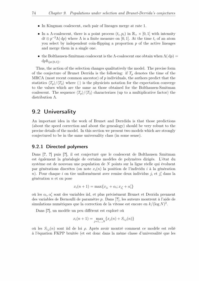
74 Chapter 9. Populations under selection and Brunet-Derrida’s conjectures

• In Kingman coalescent, each pair of lineages merge at rate 1.

• In a Λ-coalescent, there is a point process (ti, pi) in R+ × [0, 1] with intensitydt⊗ p−2Λ( dp) where Λ is a finite measure on [0, 1]. At the time ti of an atomyou select by independent coin-flipping a proportion p of the active lineagesand merge them in a single one.

• the Bolthausen-Sznitman coalescent is the Λ-coalescent one obtain when Λ( dp) =dp1p∈[0,1].

Thus, the action of the selection changes qualitatively the model. The precise formof the conjecture of Brunet Derrida is the following: if Tp denotes the time of theMRCA (most recent common ancestor) of p individuals, the authors predict that thestatistics 〈Tp〉/〈T2〉 where 〈·〉 is the physicists notation for the expectation convergeto the values which are the same as those obtained for the Bolthausen-Sznitmancoalescent. The sequence 〈Tp〉/〈T2〉 characterizes (up to a multiplicative factor) thedistribution Λ.

9.2 Universality

An important idea in the work of Brunet and Derrdida is that those predictions(about the speed correction and about the genealogy) should be very robust to theprecise details of the model. In this section we present two models which are stronglyconjectured to be in the same universality class (in some sense).

9.2.1 Directed polymers

Dans [?, ?] puis [?], il est conjecturé que le coalescent de Bolthausen Sznitmanest également la généalogie de certains modèles de polymères dirigés. L’état dusystème est de nouveau une population de N points sur la ligne réelle qui évoluentpar générations discrètes (on note xi(n) la position de l’individu i à la générationn). Pour chaque i on tire uniformément avec remise deux individus ji et j′i dans lagénération n et on pose

xi(n+ 1) = maxxji + αi;xj′i + α′i

où les αi, α′i sont des variables iid, et plus précisément Brunet et Derrida prennentdes variables de Bernoulli de paramètre p. Dans [?], les auteurs montrent à l’aide desimulations numériques que la correction de la vitesse est encore en k/(logN)2.

Dans [?], un modèle un peu différent est exploré où

xi(n+ 1) = maxj=1,...,N

xj(n) + Si,j(n)

où les Si,j(n) sont iid de loi ρ. Après avoir montré comment ce modèle est reliéà l’équation FKPP bruitée (et est donc dans la même classe d’universalité que les

9.2 Universality 75

marches aléatoires branchantes avec sélection) un cas particulier est étudié en détail(on prend la distribution de Gumbel pour ρ). Malheureusement ce cas est spécialen ce sens que la vitesse du nuage de particules diverge avec N et ne permet pas deretrouver la correction en (logN)−2.

Finallement, dans [?] le modèle suivant de polymère dirigé en champs moyen eten environement aléatoire est proposé. Chaque génération consiste en N sites quisont chacun connectés à M site choisis uniformément dans la génération précédente,2 ≤M ≤ N . Chaque lien (AB) entre deux sitesA et B porte une énergie e(A,B). Unpolymère dirigé est simplement un chemin dans la structure de graphe ainsi défini quiavance (sans saut) dans les générations. L’énergie E d’un polymère est la somme desénergies des arrêtes qu’il traverse. Le modèle est spécifié par la donnée deM et la loides e(AB). On prendra toujours des variables e(A,B) iid, des simulations numériquessont faites dans [?] pour le cas de variables uniformes sur [0, 1].On fixe à présent un site racine dans la génération 0 et pour chaque site A d’une

génération n > 0 on définit EA comme l’énergie minimale du polymère sur tous leschemins dirigés possible qui relient la racine à A. Clairement, les chemins d’énergieminimum pour un ensemble de k ≤ N sites qui appartiennent à la même générationforment un arbre à k feuilles (au moins quand n est assez grand).Les simulations effectuées dans [?] suggèrent que, comme pour les marches bran-

chantes avec sélection, cet arbre, sur une échelle de temps d’ordre (logN)3, convergevers l’arbre de Bolthausen Sznitman.Les auteurs proposent également la conjecture fascinante suivante. Les modèles

de polymères dirigés présentent une transition de phase autour d’une températurecritique. Les auteurs s’attendent donc à ce que sous cette température critiquel’arbre de Bolthausen Sznitman continue à décrire la structure des polymères, tandisqu’au dessus, la situation correspondrait aux marches aléatoires coalescentes et aucoalescent de Kingman.

9.2.2 Le lien avec l’équation FKPP bruitée

Ce paragraphe est une tentative de résumer (avec un très faible degré de précision)certains des liens qui relient l’étude de ces marches branchantes avec sélection àl’équation de FKPP bruitée.

En 1937, Fisher [?] d’une part et Kolmogorov, Petrovski et Piskunov [?] d’autrepart ont introduit l’équation aux dérivées partielles suivante qui décrit la propagationd’un front dans un milieu instable (dans le cas de Fisher il s’agissait de décrire lapropagation d’un gêne mutant dans une population)

∂tu = ∂2xxu+ u(1− u)

(je ne donne pas la version la plus générale de cette équation, en particulier on peutavoir un terme de non-linéarité différent de u(1−u)). Cette équation a des solutionsde type "onde voyageuse", et si la condition initiale décroît assez rapidement, lavitesse minimum (notée v∞) est sélectionnée.

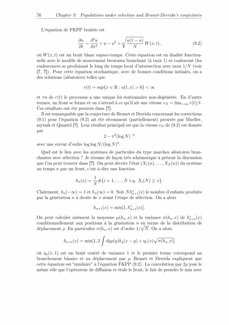
76 Chapter 9. Populations under selection and Brunet-Derrida’s conjectures

L’équation de FKPP bruitée est

∂u

∂t=∂2u

∂x2+ u− u2 +

√u(1− u)

NW (x, t), (9.2)

où W (x, t) est un bruit blanc espace-temps. Cette équation est en dualité fonction-nelle avec le modèle de mouvement brownien branchant (à taux 1) et coalescent (lescoalescences se produisant le long du temps local d’intersection avec taux 1/N (voir[?, ?]). Pour cette équation stochastique, avec de bonnes conditions initiales, on ades solutions (aléatoires) telles que

r(t) = supx ∈ R : u(t, x) > 0 <∞

et vu de r(t) le processus a une unique loi stationnaire non-dégénérée. En d’autretermes, un front se forme et on s’attend à ce qu’il ait une vitesse vN = limt→∞ r(t)/t.Ces résultats ont été prouvés dans [?].Il est remarquable que la conjecture de Brunet et Derrida concernant les corrections

(9.1) pour l’équation (9.2) ait été récemment (partiellement) prouvée par Mueller,mytnik et Quastel [?]. Leur résultat principal est que la vitesse vN de (9.2) est donnéepar

2− π2(logN)−2

avec une erreur d’ordre log logN/(logN)3.

Quel est le lien avec les systèmes de particules du type marches aléatoires bran-chantes avec sélection ? Je résume de façon très schématique à présent la discussionque l’on peut trouver dans [?]. On peut décrire l’état (X1(n), . . . , XN(n)) du systèmeau temps n par un front, c’est à dire une fonction

hn(x) =1

N#i = 1, . . . , N t.q. Xi(N) ≥ x.

Clairement, hn(−∞) = 1 et hn(∞) = 0. Soit Nh∗n+1(x) le nombre d’enfants produitspar la génération n à droite de x avant l’étape de sélection. On a alors

hn+1(x) = min[1, h∗n+1(x)].

On peut calculer aisément la moyenne µ(hn, x) et la variance σ(hn, x) de h∗n+1(x)conditionnellement aux positions à la génération n en terme de la distribution dedéplacement ρ. En particulier σ(hn, x) est d’ordre 1/

√N. On a alors

hn+1(x) = min[1, 2

∫dyρ(y)hg(x− y) + ηn(x)

√σ(hn, x)]

où ηn(x, 1) est un bruit centré de variance 1 et le premier terme correspond aubranchement binaire et au déplacement par ρ. Brunet et Derrida expliquent quecette équation est “similaire” à l’équation FKPP (9.2). La convolution par 2ρ joue lemême rôle que l’opérateur de diffusion et étale le front, le fait de prendre le min avec

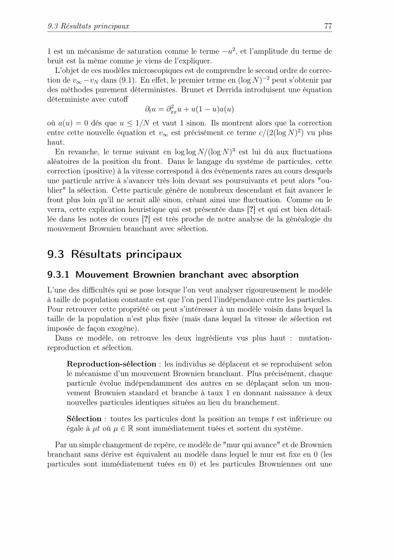
9.3 Résultats principaux 77

1 est un mécanisme de saturation comme le terme −u2, et l’amplitude du terme debruit est la même comme je viens de l’expliquer.

L’objet de ces modèles microscopiques est de comprendre le second ordre de correc-tion de v∞−vN dans (9.1). En effet, le premier terme en (logN)−2 peut s’obtenir pardes méthodes purement déterministes. Brunet et Derrida introduisent une équationdéterministe avec cutoff

∂tu = ∂2xxu+ u(1− u)a(u)

où a(u) = 0 dés que u ≤ 1/N et vaut 1 sinon. Ils montrent alors que la correctionentre cette nouvelle équation et v∞ est précisément ce terme c/(2(logN)2) vu plushaut.

En revanche, le terme suivant en log logN/(logN)3 est lui dû aux fluctuationsaléatoires de la position du front. Dans le langage du système de particules, cettecorrection (positive) à la vitesse correspond à des événements rares au cours desquelsune particule arrive à s’avancer très loin devant ses poursuivants et peut alors "ou-blier" la sélection. Cette particule génère de nombreux descendant et fait avancer lefront plus loin qu’il ne serait allé sinon, créant ainsi une fluctuation. Comme on leverra, cette explication heuristique qui est présentée dans [?] et qui est bien détail-lée dans les notes de cours [?] est très proche de notre analyse de la généalogie dumouvement Brownien branchant avec sélection.

9.3 Résultats principaux

9.3.1 Mouvement Brownien branchant avec absorption

L’une des difficultés qui se pose lorsque l’on veut analyser rigoureusement le modèleà taille de population constante est que l’on perd l’indépendance entre les particules.Pour retrouver cette propriété on peut s’intéresser à un modèle voisin dans lequel lataille de la population n’est plus fixée (mais dans lequel la vitesse de sélection estimposée de façon exogène).Dans ce modèle, on retrouve les deux ingrédients vus plus haut : mutation-

reproduction et sélection.

Reproduction-sélection : les individus se déplacent et se reproduisent selonle mécanisme d’un mouvement Brownien branchant. Plus précisément, chaqueparticule évolue indépendamment des autres en se déplaçant selon un mou-vement Brownien standard et branche à taux 1 en donnant naissance à deuxnouvelles particules identiques situées au lieu du branchement.

Sélection : toutes les particules dont la position au temps t est inférieure ouégale à µt où µ ∈ R sont immédiatement tuées et sortent du système.

Par un simple changement de repère, ce modèle de "mur qui avance" et de Brownienbranchant sans dérive est équivalent au modèle dans lequel le mur est fixe en 0 (lesparticules sont immédiatement tuées en 0) et les particules Browniennes ont une

78 Chapter 9. Populations under selection and Brunet-Derrida’s conjectures

dérive −µ (i.e. sont poussées vers 0). C’est ce modèle précisément qui va nousintéresser et que nous désignons sous le nom de mouvement Brownien branchantavec absorption en 0 (on note parfois kBBM(µ) pour killed Brownian motion withdrift (−µ)). (voir les figures 9.2 et 9.3 qui sont reproduites de la thèse de DamienSimon avec son aimable autorisation).Ce modèle, dont l’étude remonte au moins à Kesten [?] a fait l’objet de travaux

récents de Derrida et Simon [?, ?] dans lesquels une conjecture (étayée par une analyseperturbative de l’équation aux dérivées partielle de FKPP qui peut sans doute êtrerendue rigoureuse) concernant la probabilité de survie est formulée.

9.3.2 Survie

Dans la suite on notera Px et Ex pour désigner la loi (et l’espérance sous cette loi) dukBBM qui a pour état initial une particule unique en position x > 0. On ne précisepas µ qui est en général fixé. Dans [?], Kesten montre un premier résultat simple surla survie du processus, qui dans notre cadre peut s’énoncer ainsi :

Theorem 87 (Kesten, [?]). Si µ ≥√

2 le processus s’éteint presque sûrement entemps fini (cas critique et sous-critique).Si µ <

√2 le processus survit avec probabilité positive et dans ce cas le nombre de

particules en vie croît exponentiellement (cas sur-critique). Dans ce cas on noteQµ(x) la probabilité sous Px que le processus survive.

Plus récemment, quelques résultats supplémentaires ont été obtenus :

• Harris, Harris, et Kyprianou [?] montrent (cf. Théorème 13) que, pour µ <√

2,la fonction x 7→ Qµ(x) satisfait l’équation de Kolmogorov

1

2Q′′µ(x)− µQ′µ(x) = Qµ(x)(1−Qµ(x))

avec conditions aux bords limx→0Qµ(x) = 0 et limx→∞Qµ(x) = 1. Ils montrentégalement (cf. Théorème 1) que pour chaque µ <

√2 fixé il y a une constante

K telle quelimx→∞

e(√µ2+2−µ)x(1−Qµ(x)) = K.

• Dans le cas sous-critique (µ >√

2) Harris et Harris [?] utilisent des techniquesde martingales et de décomposition en épine dorsale pour calculer les asymp-totiques de Px(ζ > t) quand t devient grand (et où ζ est l’instant d’extinctiondu processus).

• Dans [?] Simon et Derrida obtiennent des estimées pour la probabilité de survieQµ(x). Ils conjecturent qu’il existe K tel que quand L− x 1,

Qµ(x) = KLe√

2(x−L)

(sin

(πx

L

)+O

(1

L2

))+O(e2

√2(x−L))

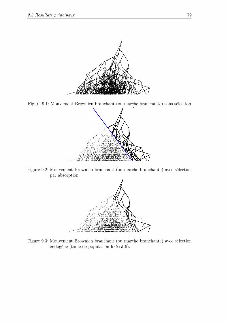
9.3 Résultats principaux 79

Figure 9.1: Mouvement Brownien branchant (ou marche branchante) sans sélection

Figure 9.2: Mouvement Brownien branchant (ou marche branchante) avec sélectionpar absorption

Figure 9.3: Mouvement Brownien branchant (ou marche branchante) avec sélectionendogène (taille de population fixée à 6).

80 Chapter 9. Populations under selection and Brunet-Derrida’s conjectures

(équation (B.16)) et qu’il existe une autre constante c telle que quand x > Lou L− x est O(1),

Qµ(x) = 1− θ(x− L+ c) +O

(1

L2

),

où θ résout l’équation différentielle (9.3) ci-dessous (équation (B.17)). Cesestimées sont obtenues à l’aide de méthodes entièrement analytiques qui nesont cependant pas encore un argument tout à fait rigoureux.

On pose ε =√

2 − µ > 0, et on définit L par la relation 1 − µ2/2 − π2/2L2 = 0,c’est-à-dire L = π/

√2− µ2 = π/

√ε. Le théorème suivant que nous obtenons dans

[?] valide les prédictions de Derrida et Simon.

Theorem 88 (B.,Berestycki,Schweinsberg [?]). Soit α ∈ R fixé. Alors il existe unefonction θ : R→ R telle que

limε→0

Qµ(L+ α) = θ(α),

où θ : R→ (0, 1) satisfait1

2θ′′ −

√2θ′ = θ(1− θ). (9.3)

Il existe une constante C telle que si L− x 1, alors

Qµ(x) ∼ CLe−µ(L−x) sin

(πx

L

),

où ∼ désigne l’équivalence asymptotique quand ε→ 0.

La preuve de ce résultat (dont je donne les grandes lignes plus loin) utilise lesrésultats que nous avons obtenus dans [?] et que je présente maintenant.

9.3.3 Généalogie et CSBP de Neveu

La présentation de ces résultats est légèrement modifiée par rapport à [?] ou unparamètrage différent est utilisé. Dans toute cette partie, pour chaque ε donné ontravail sous la loi Px où l’on fixe x = L. On se fixe n ≥ 1 et l’on définit le processus dela partition ancestrale (Πε

s, 0 ≤ s ≤ t) à valeur dans Pn (les partitions de 1, . . . , n)en tirant uniformément n individus dans la populations au temps tε−3/2 et en posantque i et j sont dans le même bloc de Πε

s si et seulement si les individus i et j ont lemême ancêtre au temps (t− s)ε−3/2.

Theorem 89 (B.,Berestycki,Schweinsberg [?]).

(Πεs, 0 ≤ s ≤ t)

fdd→ε0

(Π23/2π3s, 0 ≤ s ≤ t)

où Π est le coalescent de Bolthausen-Sznitman restreint à 1, . . . , n.

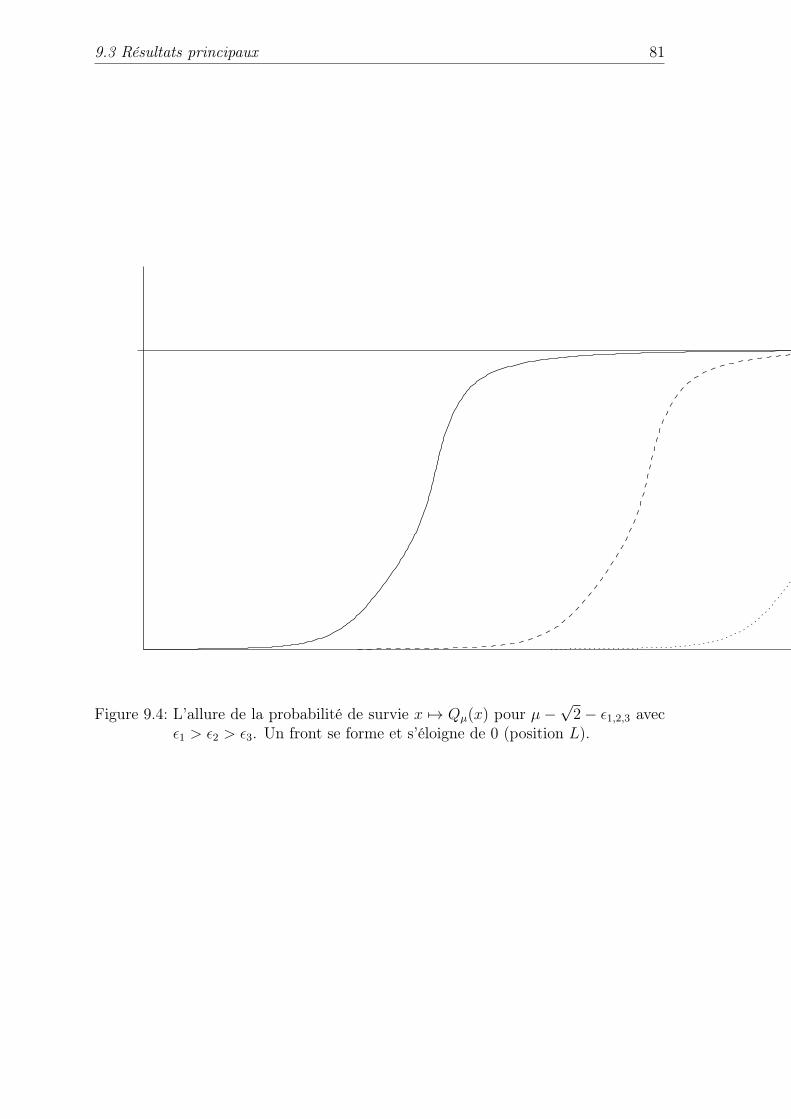
9.3 Résultats principaux 81

Figure 9.4: L’allure de la probabilité de survie x 7→ Qµ(x) pour µ−√

2− ε1,2,3 avecε1 > ε2 > ε3. Un front se forme et s’éloigne de 0 (position L).

82 Chapter 9. Populations under selection and Brunet-Derrida’s conjectures

En outre, si l’on appelle M εt le nombre de particules en vie au temps t on a

Theorem 90 (B.,Berestycki,Schweinsberg [?]).(1

ε3/2eπ√

2/εM ε

tε−3/2 , t ≥ 0

)fdd→ε0

(Zt, t ≥ 0)

où Z est un CSBP de mécanisme de branchement ψ(u) = au+ 2π2u log u, pour unecertaine constante a ∈ R, issu d’une population initiale Z0 aléatoire de loi connue.

Le Gall et Bertoin avaient déjà observé dans [?] que la généalogie du CSBP deNeveu (de mécanisme de branchement ψ(u) = u log u) était donné par le coalescentde Bolthausen-Sznitman. Ainsi, si l’on peut montrer que la population évolue selonune version du CSBP de Neveu il n’est pas surprenant que sa généalogie soit donnéepar le coalescent de Bolthausen-Sznitman.La renormalisation que l’on utilise dans le résultat ci-dessus montre que si l’on

veut avoir de l’ordre de N particules en vie il faut prendre ε3/2eπ√

2/ε N soit ε ∼2π2/(logN+3 log logN)2. On peut ainsi décider de paramètrer entièrement le modèlepar N en prenant µN =

√2− 2π2

(logN+3 log logN)2 et L = (logN + 3 log logN)/√

2.

L’un des résultats clés dans [?] consiste à montrer que l’on peut mesurer la taille dela population en attribuant des poids aux individus tout en conservant la convergencedu Théorème 90 vers le CSBP de Neveu (avec une renormalisation différente). Plusprécisément, si l’on définit

ZN(t) :=

MN (t)∑i=1

eµXi(t) sin(πXi(t)/L)1Xi(t)≤L, t ≥ 0,

on a alors le résultat suivant

Theorem 91 (B.,Berestycki,Schweinsberg [?]). Sous Px on a(ZN(t)

N(logN)2, t ≥ 0

)fdd→ε0

(Zt, t ≥ 0)

où Z est un CSBP de mécanisme de branchement ψ(u) = au + 2π2u log u pour unecertaine constante a ∈ R issu d’une population initiale Z0 aléatoire de loi connue.

Dans [?] nous ne travaillons pas sous Px, nous formulons le Théorème ci-dessus pourune suite de configuration initiales X1(0), . . . , XMN (0)(0) telles que ZN(0)/N(logN)2

converge en distribution vers une certaine variable W non-dégénérée et tels queYN(0) = o(N(logN)3) avec

YN(t) :=

MN (t)∑i=1

eµXi(t), t ≥ 0.

9.3 Résultats principaux 83

Dans ce cas W est bien sûr la loi de la population initiale Z0. Pour prouver lesThéorèmes 90 et 91 tels que je les énonce ici, il faut donc montrer que si l’on démarreavec une particule en L, alors en un temps très court (négligeable devant (logN)3) lesystème se trouve dans une configuration X1, . . . , XN (où N est aléatoire) telle quepour ces position ZN/N(logN)2 converge en distribution et YN = o(N(logN)3). Laloi limite de ZN/N(logN)2 donne la loi initiale de Z0 qui est mentionnée dans lesrésultats ci-dessus.

9.3.4 Quelques idées de la preuve des Théorèmes 89, 90 et 91

Notre approche dans [?] consiste à traiter séparément les particules qui atteignentune distance d’ordre L du mur en 0. Ces particules sont assez loin pour ne plus"sentir" le mur et ainsi peuvent rapidement produire une grande descendance, ce quiconduit à un saut positif de la taille de la population et à des coalescences multiplesde lignées ancestrales lorsque l’on remonte le temps.Cette approche est à comparer à la description phénoménologique du modèle à

population constante que donnent Derrida et ses coauteurs (dans [?, ?] ou dans lesnotes du mini-cours que Eric Brunet a donné à Marseille en 2007 [?]). Ils montrentcomment la correction de deuxième ordre à la vitesse (le terme en log logN/(logN)3)est due à des événements rares durant lesquels une particule se retrouve en avancedu front et produit une grande descendance avant d’être rattrapée, créant ainsi unefluctuation dans la position du front.

Pour commencer, on peut considérer un mouvement Brownien branchant danslequel les particules sont tuées lorsqu’elles atteignent 0 ou L. Si la configurationinitiale consiste en une seule particule en position x, alors, pour t assez grand, ladensité de particules attendue autour du point y est approximativement pt(x, y) dy,où

pt(x, y) =2

Le(1−µ2/2−π2/2L2)t · eµx sin

(πx

L

)· e−µy sin

(πy

L

). (9.4)

On peut tirer plusieurs informations sur le comportement du mouvement Brownienbranchant dans une bande de cette formule. Le paramètre t n’apparaît que dans lepremier facteur exponentiel. La taille de la population devrait donc rester stable désque 1 − µ2/2 − π2/2L2 = 0 (ce qui correspond en effet à notre choix). Une secondeobservation est que la densité est proportionnelle à eµx sin(πx/L), c’est-à-dire, ensommant sur toutes les particules au temps t, à ZN(t). On voit donc que ZN(t)est un bon prédicteur du nombre de particules que l’on trouvera dans un ensembleà un certain temps futur. Ainsi, ZN(t) est la bonne façon de mesurer la "taille"de la population. Enfin, la densité est également proportionnelle à e−µy sin(πy/L).En conséquence, dés que t est assez grand (d’ordre (logN)2) le système a "oublié"sa configuration initiale et les particules sont dans une configuration stable dont ladensité de particules à y est proportionnelle à e−µy sin(πy/L).L’étape suivante consiste à observer qu’une particule qui atteint L conduit à un

"saut" dans la taille de la population. En effet, si l’on démarre avec N particules

84 Chapter 9. Populations under selection and Brunet-Derrida’s conjectures

tirée selon cette densité d’équilibre entre 0 et L, alors ZN(0) vaut approximativement

N

∫ L

0

eµy sin

(πy

L

)· CLe−µy sin

(πy

L

)dy,

qui est d’ordre NL2. D’autre part, si on part avec une particule en L, ses descendantsn’iront typiquement pas plus loin qu’une constante à droite de L. Pour estimer lacontribution typique d’une particule en L au temps t on utilise (9.4) avec L à la placede x et L + α au lieu de L, avec α > 0 une constante. La valeur de ZN(t) doit êtredu même ordre que∫ L

0

eµy sin

(πy

L

)· 2

L+ αeµL sin

(πL

L+ α

)e−µy sin

(πy

L+ α

)dy,

qui est d’ordre L−1eµL. En utilisant l’expression de L en fonction de N on obtientdes ordres de grandeur identiques. Une particule à L produit donc une augmentationsubstantielle de la taille de la population.

Pour traiter les particules qui n’atteignent pas L, nous commençons par étudierun mouvement Brownien branchant tué en 0 et en LA

LA =1√2

(logN + 3 log logN − A

), (9.5)

À l’aide de (9.4), nous obtenons des estimées pour les premiers et deuxièmes momentsde différentes quantités ce qui nous permet ensuite de calculer le premier et deuxièmemoment de ZN(t) conditionnellement à l’état du processus θ(logN)3 unités de tempsavant. La borne du second moment est suffisante pour établir une loi des grandnombres quand A est grand qui permet de contrôler la distance entre ZN(t) et samoyenne. La troncation à LA est nécessaire car sinon les moments seraient dominéspar des événements rares où une particule arrive très loin à droite et produit unegrande descendance qui survit.

L’étape suivante consiste à compter le nombre de particules qui atteignent LA. Onpeut montrer que si l’on part de N particules dans leur configuration stable, alors ilfaut attendre environs (logN)3 unités de temps pour voir une particule qui atteintLA. On peut se convaincre qu’il s’agit de la bonne échelle de temps avec l’argumentheuristique suivant. Si β > 0 est une constante, alors le nombre de particules entreL− β et L au temps t est d’ordre

N

∫ L

L−βCLe−µy sin

(πy

L

)dy,

c’est-à-dire d’ordre 1/(logN)3. Chacune de ces particules a une probabilité positived’atteindre L entre t et t + 1 mais on peut montrer que les particules qui sont àune distance de L plus grande qu’une constante ne touche L avant t+ 1 qu’avec une

9.3 Résultats principaux 85

faible probabilité. On a donc O(1/(logN)3) particules qui atteignent L par unité detemps.

Lorsqu’une particule atteint LA, elle pourrait avoir branché juste avant de toucherLA permettant ainsi à un grand nombre de particules d’atteindre elles aussi LA.On doit donc contrôler le second moment de ce nombre. Á cette fin on montre queconditionnellement à ce qu’au moins une particule atteigne LA, l’espérance du nombrede particules qui atteignent LA dans un intervalle de temps de durée θ(logN)3, estbornée par une constante.

La clé pour analyser la contribution des particules qui atteignent LA se trouvedans un résultat de Neveu [27]. Si une particule démarre à LA et y est une grandeconstante, alors le nombre de descendants qui atteignent LA − y est y−1e

√2yW , où

W est une variable aléatoire. À l’aide de théorèmes Taubériens nous démontronsque pour x grand l’on a P (W > x) ∼ B/x. C’est ce résultat qui conceptuellementexplique pourquoi la généalogie est décrite par un coalescent de Bolthausen-Sznitman.La contribution d’une particule en LA sera approximativement proportionnelle auxnombre de ses descendants qui atteignent LA− y pour y assez grand. La probabilitéqu’une particule en LA produise un saut de taille au moins x est ainsi proportionnelleà 1/x ce qui entraîne que la mesure de Lévy du CSBP limite aura une densitéproportionnelle à x−2 comme dans le cas du CSBP de Neveu, conduisant ainsi aurésultat de dualité avec le coalescent de Bolthausen-Sznitman. Techniquement, lapreuve du Théorème 89 se fait en utilisant les flots de ponts introduits par Bertoinet Le Gall dans [?].

9.3.5 Un bref aperçut de la preuve du Théorème 88

L’essentiel du travail pour montrer le Théorème 88 consiste à montrer que pour αfixé, la quantité Qµ(L + α) converge vers une limite appelée θ(α) quand ε → 0.Le Théorème 88 montre que si l’on démarre avec une particule en L, le processusMN(t) du nombre de particules, une fois renormalisé, converge vers une CSBP deNeveu (Zt, t ≥ 0) issu d’une population initiale de taille W où W est la variablelimite de Neveu que l’on vient de voir. Les trajectoires du CSBP de Neveu issu d’unepopulation initiale x sont de deux types : soient elles croissent sur-exponentiellement,soit elles convergent vers 0 (mais n’atteignent pas 0 en temps fini). Si le mécanismede branchement est ψ(u) = au + bu log u La probabilité de ce second événementest e−bx. Tout le travail consiste donc à montrer que la probabilité d’extinction duprocessus (MN(t), t ≥ 0) converge bien vers E(e−bW ) la probabilité que le processuslimite (Zt, t ≥ 0) converge vers 0. Si on démarre avec une particule en L + α àprésent, les mêmes arguments montrent que la probabilité d’extinction converge versE(e−be

√2αW ) et l’on sait déjà que cette fonction de α résout l’équation KPP (9.3).

La seconde partie du théorème qui concerne le comportement de Qµ(x) pour x fixése fait selon les grandes lignes suivantes. Partant d’une particule à x on compte lenombre R de particules qui touchent L− α si on tue les particules à cet instant. On

86 Chapter 9. Populations under selection and Brunet-Derrida’s conjectures

peut monter que

Ex[R] =e√

2α

π√

2αeµx sin

(πx

L− α

)1

N(logN)2(1 + CN,α)

où pour chaque α > 0, CN,α → 0 quand N → ∞. Une borne sur le second momentde R permet alors de conclure que

Qµ(x) =e√

2α

π√

2α· eµx sin

(πx

L

)· 1

N(logN)2·Qµ(L− α)(1 + CN,α + o(α−1)),

où o(α−1) est un terme qui tends vers 0 quand α→∞ et est uniforme en N . Il suffitmaintenant d’appliquer la première partie du théorème pour conclure.

Chapter 10Branching Brownian motion withabsorption: The critical case

87

Bibliography

[1] Aïdékon, E. (2013). Convergence in law of the minimum of a branching randomwalk. Ann. Probab. Volume 41, Number 3A (2013), 1362-1426.

[2] E. Aïdékon, J. Berestycki, E. Brunet, and Z. Shi. (2013) Branching Brownianmotion seen from its tip. Probab. Theor. Rel. Fields, Volume 157, Issue 1-2, pp405-451

[3] Arguin, L.-P., Bovier, A. and Kistler, N. (2011). The genealogy of extremalparticles of branching Brownian motion. Comm. Pure Appl. Math. Volume 64,Issue 12, pages 1647?1676,

[4] Arguin, L.-P., Bovier, A. and Kistler, N. (2012). Poissonian statistics in theextremal process of branching Brownian motion. Ann. Appl. Probab. Volume22, Number 4, 1693-1711.

[5] Arguin, L.-P., Bovier, A. and Kistler, N. (2013). The extremal process of branch-ing Brownian motion. Probab. Theory and Rel. Fields, Volume 157, Issue 3-4,pp 535-574

[6] Bramson, M. (1978), Maximal displacement of branching Brownian motion,Comm. Pure Appl. Math., 31, 5, 531–581.

[7] Bramson, M. (1983). Convergence of solutions of the Kolmogorov equation totravelling waves. Mem. Amer. Math. Soc. 44, no. 285.

[8] Brunet, E. and Derrida, B. (2009). Statistics at the tip of a branching randomwalk and the delay of traveling waves. Europhys. Lett. 87, 60010.

[9] Brunet, E. and Derrida, B. (2010). A branching random walk seen from the tip.ArXiv cond-mat/1011.4864

[10] Chauvin, B. and Rouault, A. (1988). KPP equation and supercritical branchingBrownian motion in the subcritical speed area. Application to spatial trees.Probab. Theory Related Fields 80, 299–314.

89

90 Bibliography

[11] B. Chauvin, (1991). Multiplicative martingales and stopping lines for branchingBrownian motion, Ann. Probab. 30 1195?1205.

[12] Gantert, N., Hu, Y. and Shi, Z. (2011). Asymptotics for the survival probabilityin a killed branching random walk. Ann. Inst. H. Poincaré Probab. Statist. 47,111–129.

[13] Friedman, A. (1964). Partial Differential Equations of Parabolic Type. Prentice-Hall.

[14] Hardy, R., and Harris, S. C. (2006) A new formulation of the spine approach tobranching diffusions. arXiv: 0611.054 [math.PR] .

[15] Harris, S.C. (1999). Travelling-waves for the FKPP equation via probabilisticarguments. Proc. Roy. Soc. Edin. 129A, 503–517.

[16] Harris, J.W., Harris, S.C. and Kyprianou, A.E. (2006). Further probabilis-tic analysis of the Fisher-Kolmogorov-Petrovskii-Piscounov equation: one-sidedtraveling waves. Ann. Inst. H. Poincaré Probab. Statist. 42, 125–145.

[17] Harris, S. C., and Roberts, M. I. (2011) The many-to-few lemma and multiplespines. arXiv:1106.4761 [math.PR].

[18] Harris, J.W. and Harris, S.C. (2007). Survival probabilities for branching Brow-nian motion with absorption. Electronic Commun. Probab. 12, 81–92.

[19] Hu, Y. and Shi, Z. (2009). Minimal position and critical martingale convergencein branching random walks, and directed polymers on disordered trees. Ann.Probab. 37, 742–789.

[20] Ikeda, N., Nagasawa, M. and Watanabe, S. (1965). On branching Markov pro-cesses. Proc. Japan Acad. 41, 816–821.

[21] Kyprianou, A. (2004). Travelling wave solutions to the K-P-P equation: alter-natives to Simon Harris’ probabilistic analysis. Ann. Inst. H. Poincaré Probab.Statist. 40, 53–72.

[22] Lalley, S.P. and Sellke, T. (1987). A conditional limit theorem for frontier of abranching Brownian motion. Ann. Probab. 15, 1052–1061.

[23] Lyons, R. (1997). A simple path to Biggins’ martingale convergence forbranching random walk. In: Classical and Modern Branching Processes (Eds.:K.B. Athreya and P. Jagers). IMA Volumes in Mathematics and its Applications84, 217–221. Springer, New York.

[24] McKean, H.P. (1975). Application of Brownian motion to the equation ofKolmogorov-Petrovskii-Piskunov. Comm. Pure Appl. Math., 28, 323–331.

[25] Madaule, T. (2011). Convergence in law for the branching random walk seenfrom its tip. arXiv:1107.2543 [math.PR]

Bibliography 91

[26] Maillard, P. (2011). A characterisation of superposable random measures.arXiv:1102.1888 [math.PR]

[27] Neveu, J. (1988). Multiplicative martingales for spatial branching processes.In: Seminar on Stochastic Processes, 1987 (Princeton, NJ, 1987), pp 223–242,Progr. Probab. Statist., 15, Birkhäuser, Boston.

[28] M. Roberts (2013) A simple path to asymptotics for the frontier of a branchingBrownian motion. Ann. probab. Volume 41, Number 5 (2013), 3518-3541.

[29] Resnick, S.I. (1987). Extreme Values, Regular Variation, and Point Processes,Applied Probability Series 4, Springer-Verlag.