PHD THESIS:

Topics in Ballistic and Transient Conditions

for Random Walks in Random Environments

A Thesis submitted by Enrique Guerra Aguilar for the degree of Doctor

en Matematicas in the Pontificia Universidad Catolica de Chile

Supervised by:

Alejandro F. Ramırez

July, 2016

Santiago, Chile

Dedicado a mi esposa Stephanie Alfaro y a mis padres

Enrique Guerra Galaz y Patricia Aguilar Jara.

i

Acknowledgements

I would here like to thank all people responsible for making this thesis more than a simple

keyboard work. First of all, I express my sincere thanks to my thesis advisor Alejandro

Ramırez for letting me to be his student. It was a real pleasure to work with him, I learnt

much more than mathematics. He is undoubtedly my mentor and all my results were

turned out by a deep exchange of probabilistic ideas. I also thank my thesis committee:

Joaquin Fontbona, Gregorio Moreno, Rolando Rebolledo and Christophe Sabot. I offer my

apologies for the delay in delivering the final thesis version. I have studied for more than

a decade at the Pontificia Universidad Catolica de Chile. There I have met and interacted

with many people. Among friends and staff whom I met, I would like to especially thank

Dr. Moreno and Dr. Cabezas for sharing their knowledge through which often made

me strengthen my own knowledge and like for the probability field. Also, I thank my

office mate Alvaro Ferrada for his friendship, who is my friend from the very beginning of

my graduate studies. I thank the partial support throughout my research to the Nucleo

Milenio: Modelos Estocasticos de Sistemas Complejos y Desordenados, a mathematical

community based at the Pontificia Universidad Catolica and the Universidad de Chile.

Regarding the Nucleo staff, for the constant help in non-mathematical matters I express

my gratitude to: Consuelo Thiers, Maria Eugenia Heckman and Cecile Jourdan. Last

but most important, I deeply thank with all of my heart my family: my wife Stephanie

Alfaro who is the main source of inspiration in each mathematical idea that I have, and

my parents: Enrique Guerra and Patricia Aguilar whom I owe all what I am.

ii

Abstract

This thesis is devoted to the study of the stochastic process model called Random Walk

in Random Environment (RWRE). To be precise, our research focuses on two kinds of

random environments. The first one is the so called uniformly elliptic i.i.d. random

environment. In this model it is conjectured that in dimensions d ě 2 any random walk

which is directionally transient is ballistic. The ballisticity conditions for RWRE somehow

interpolate between directional transience and ballisticity and have served to quantify the

gap which one needs to answer affirmatively this conjecture. Two important ballisticity

conditions introduced by Sznitman [Sz02] in 2001 and 2002 are the so called conditions

pT 1q and pT q: given a slab of width L orthogonal to l, condition pT 1q in direction l is

the requirement that the annealed exit probability of the walk through the side of the

slab in the half-space tx : x ¨ l ă 0u, decays faster than e´CLγ

for all γ P p0, 1q and some

constant C ą 0, while condition pT q in direction l is the requirement that the decay is

exponential e´CL. It is believed that pT 1q implies pT q. We show that pT 1q implies at least

an almost (in a sense to be made precise) exponential decay. The second class of random

environment to be studied is a larger class which only requires a mixing condition on the

environment law. As a matter of fact, the ballisticity conditions in this framework are not

well-understood. Therefore our purpose is to find a connection between this strictly larger

class of environments and the ballisticity conditions which have proved to be a powerful

theoretical concept for random walks in an i.i.d. random environment. In that direction,

we prove that every random walk in a uniformly elliptic random environment satisfying

the cone mixing condition and a non-effective polynomial ballisticity condition with high

enough degree has an asymptotic direction.

iii

Contents

Acknowledgements ii

Abstract. iii

List of Figures vi

General Introduction 1

0.1 Some well-known results in uniformly elliptic i.i.d. random environments.

(under d ě 2.) . . . . . . . . . . . . . . . . . . . . . . . . . . . . . . . . . . 6

0.1.1 On Kalikow’s Condition. . . . . . . . . . . . . . . . . . . . . . . . . 6

0.1.2 Ballisticity Conditions: Stretched Exponential Decay, Effective Cri-

terion and Polynomial Condition . . . . . . . . . . . . . . . . . . . 9

0.2 Previous results for random walks in cone mixing random environments . . 13

0.3 A brief explanation of the Thesis Results . . . . . . . . . . . . . . . . . . . 17

0.3.1 Main Result for i.i.d. Random Environments . . . . . . . . . . . . . 17

0.3.2 Main Result for cone mixing random environments . . . . . . . . . 18

1 Almost exponential decay for the exit probability from slabs of ballistic

RWRE 21

1.1 Introduction . . . . . . . . . . . . . . . . . . . . . . . . . . . . . . . . . . . 21

1.2 Proof of Theorem 1.1.2 . . . . . . . . . . . . . . . . . . . . . . . . . . . . . 26

1.2.1 Preliminaries and notation . . . . . . . . . . . . . . . . . . . . . . . 27

1.2.2 The maximal growth condition on scales . . . . . . . . . . . . . . . 29

1.2.3 An adequate choice of fast-growing scales . . . . . . . . . . . . . . . 32

1.2.4 The effective criterion implies Theorem 1.1.2 . . . . . . . . . . . . . 38

iv

2 Asymptotic Direction for Random Walk in Strong Mixing Environment 45

2.1 Introduction . . . . . . . . . . . . . . . . . . . . . . . . . . . . . . . . . . . 45

2.2 Preliminary discussion . . . . . . . . . . . . . . . . . . . . . . . . . . . . . 51

2.2.1 Non-effective polynomial condition and its relation with other di-

rectional transience conditions . . . . . . . . . . . . . . . . . . . . . 51

2.2.2 Cone mixing and ergodicity . . . . . . . . . . . . . . . . . . . . . . 54

2.2.3 Polynomial Decay implies Polynomial decay in a neighborhood . . . 56

2.3 Examples of directionally transient random walks without an asymptotic

direction and vanishing velocity . . . . . . . . . . . . . . . . . . . . . . . . 61

2.3.1 Random walk with a vanishing velocity but with an asymptotic

direction . . . . . . . . . . . . . . . . . . . . . . . . . . . . . . . . . 62

2.3.2 Directionally transient random walk without an asymptotic direction 65

2.4 Backtracking of the random walk out of a cone . . . . . . . . . . . . . . . . 69

2.5 Polynomial control of regeneration positions . . . . . . . . . . . . . . . . . 77

2.5.1 Preliminaries . . . . . . . . . . . . . . . . . . . . . . . . . . . . . . 77

2.5.2 Preparatory results . . . . . . . . . . . . . . . . . . . . . . . . . . . 82

2.5.3 Proof of Proposition 2.5.3 . . . . . . . . . . . . . . . . . . . . . . . 87

2.6 Proof of Theorem 2.1.1 . . . . . . . . . . . . . . . . . . . . . . . . . . . . . 98

2.6.1 Approximate regeneration time sequence . . . . . . . . . . . . . . . 98

2.6.2 Approximate asymptotic direction . . . . . . . . . . . . . . . . . . . 102

2.6.3 Proof of Theorem 2.1.1 . . . . . . . . . . . . . . . . . . . . . . . . . 105

2.7 Appendix . . . . . . . . . . . . . . . . . . . . . . . . . . . . . . . . . . . . 108

v

List of Figures

1 Cone . . . . . . . . . . . . . . . . . . . . . . . . . . . . . . . . . . . . . . . 3

2.1 The choice of boxes. . . . . . . . . . . . . . . . . . . . . . . . . . . . . . . 58

2.2 A geometric sketch to bound Q2rXTBL,2L,l p0qR B`BL,2L,lp0qs. . . . . . . . . . 69

2.3 The boxes By and Bz are inside of Cp0, l, αq. . . . . . . . . . . . . . . . . . 85

vi

General Introduction

Random Walk in a Random Environment (RWRE) is a classical model of random motion

in a random media. It was originally introduced as a toy model for replication of DNA

chains and phase transition in alloys. We can describe a d- dimensional RWRE as the

canonical Markov chain pXnqně0 with state space Zd, where its transition probabilities to

nearest neighbor sites are random. In spite of its simplicity, when the dimension is larger

than 1 its asymptotic laws are still not well-understood. This problem, is essentially due

to the reversibility loss in the chain on averaging over the environment. Consequently

this makes it hard to apply standard convergence methods in order to get asymptotic

laws. Some progress has been done in that direction by means of the introduction of what

are called ballisticity conditions. These conditions are essentially a functional control

(for instance a polynomial control) of the probability that the walk exits from large slabs

transversal to directions l1 in a neighborhood of a given direction l P Sd´1 by the unlikely

slab boundary side: the one which is in the direction ´l1. The study of ballisticity

conditions is the main focus of this thesis. To appropriately introduce them, we will now

explain more precisely the model. Let d ě 1 be a positive integer which will be thought

as the underlying random walk dimension. We consider the p2d´1q- dimensional simplex

P defined by:

P :“ tz P R2d :2dÿ

i“1

zi “ 1, zi ě 0 for i P r1, 2dsu.

Now, an environment ω :“ ωpx, eq|xPZd,ePZd,|e|“1 is an element of the set Ω :“ pPqZd which

specifies at each site x P Zd the transition probabilities of the walk. Throughout this

chapter, by canonical σ- algebra on a product space we mean the σ-algebra generated

by the cylinder measurable sets. For the time being, we assume that we have a given

probability measure P on the canonical σ- algebra W in Ω.

1

For fixed ω P Ω and x P Zd, one defines the quenched law Px,ω, as the law of the

canonical Markov chain pXnqně1 starting from x, with state space Zd and satisfying

Px,ωrX0 “ xs “ 1

Px,ωrXn`1 “ Xn ` e | Xn, Xn´1, . . . X0s “ ωpXn, eq for e P Zd, |e| “ 1.

We call F the canonical σ- algebra in pZdqN, which is the σ- algebra in the walk path

space. Furthermore, for a prescribed probability measure P one then defines the annealed

or averaged law Px as the semi-direct product Pb Px,ω on W ˆ F .

We consider two types of random environments: the first one will be the so-called

i.i.d. random environment framework; the second one is a larger class satisfying a mixing

condition. We start by defining the i.i.d. random environment. Let κ P p0, 12ds and µ be

a probability measure on P such that for each x P Zd, ωpx, ¨q distributes as µ, and µ is

supported on the subset Pκ of P defined by:

Pκ :“ tz P R2d :2dÿ

i“1

zi “ 1, zi ě κ for i P r1, 2dsu.

This last restriction on the support of the law µ is called uniform ellipticity assump-

tion. The random environment is now an element of the measurable probability space

Ωκ :“ pPκqZd

which is endowed with canonical σ´ algebra Wκ and the product measure

P :“ µbZd. For the easy of notation, we shall drop κ when we talk about i.i.d random

environments.

Before introducing the cone mixing condition we weaken the uniform ellipticity as-

sumption. We say that P is uniformly elliptic with respect to l, denoted by pUEq|l, if the

jump probabilities of the random walk are positive and larger than 2κ in those directions

for which the projection on l is positive. In other words if Prωp0, eq ą 0s “ 1 for |e| “ 1

and if

P”

minePE

ωp0, eq ě 2κı

“ 1,

where

E :“dď

i“1

tsgnpliqeiu ´ t0u (1)

2

and by convention sgnp0q “ 0.

It will be convenient to define what is understood by a cone in this work. We let α be a

small positive real number and R be a rotation such that

Rpe1q “ l. (2)

To define the cone, it will be useful to consider for each i P r2, ds, the directions

l`i “l ` αRpeiq

|l ` αRpeiq|and l´i “

l ´ αRpeiq

|l ´ αRpeiq|.

The cone Cpx, l, αq centered in x P Rd is defined as

Cpx, l, αqq :“dč

i“2

z P Rd : pz ´ xq ¨ l`i ě 0, pz ´ xq ¨ l´i ě 0(

. (3)

The following picture shows a cone centered at x in the lattice Z2

x

β = arctan(α)

C(x, l, α)

l

Figure 1: Cone

We are ready to state the cone mixing condition. Define the canonical shifts tθx : x P

Zdu by θxωpyq :“ ωpx ` yq for all ω P Ω and x, y P Zd. Let us first recall the concept

of ergodic measure. We say that a probability measure P is stationary if for all x P Zd

and A P W one has that Ppθ´1x Aq “ PpAq. We say that P is ergodic, if whenever A P W

is such that A “ θ´1x A for all x P Zd, one has that PpAq “ 0 or that PpAq “ 1. Now,

let φ : r0,8q Ñ r0,8q with limrÑ8 φprq “ 0. We say that a stationary probability

measure P satisfies the cone mixing assumption with respect to α, l and φ, denoted

3

pCMqα,φ|l if for every pair of events A,B, where PpAq ą 0, A P σtωpz, ¨q; z ¨ l ď 0u, and

B P σtωpz, ¨q; z P Cprl, l, αqu, it holds that

ˇ

ˇ

ˇ

ˇ

PrAXBsPrAs

´ PrBsˇ

ˇ

ˇ

ˇ

ď φpr|l|1q. (4)

Thus, we can consider assumption pCMqα,φ|l as a restriction on the P- dependence. As it

was mentioned in [CZ01], it is important to allow strictly positive angles β :“ arctanpαq.

Otherwise, when β “ 0 and the cone mixing assumption is satisfied for each l P Sd´1, then

the measure P is actually a finite range dependence law (see [Ze1] and [B1]). Furthermore,

whenever a probability measure P satisfies the cone mixing assumption, it is ergodic (this

will be proved in Chapter 2).

We will be dealing with three important asymptotic concepts:

• We say that the walk is transient in the direction l, if

P0

”

limnÑ8

Xn ¨ l “ 8ı

“ 1. (5)

• We say that the walk is ballistic in the direction l if

P0

„

lim infnÑ8

Xn ¨ l

ną 0

“ 1. (6)

Moreover, in this case we will also say that the walk has ballistic behavior.

• We say that a non-zero d- dimensional deterministic vector v is an asymptotic di-

rection for the walk if

P0

„

limnÑ8

Xn

|Xn|Ñ v

(7)

holds.

It is straightforward to see that any RWRE which is ballistic in direction l is transient

in the same direction. In the 1 dimensional case, the walk asymptotic behavior is well-

understood, and the results come from Smith-Wilkinson [SW69], Solomon [So75] and Alili

[Al99]. Define

ρ :“ωp0,´e1q

ωp0, e1q.

We then have the following transience criteria:

4

Theorem 0.0.1 (Smith-Wilinson, Solomon, Alili). Suppose that P is ergodic and that

Erlnpρqs is defined (possibly ˘8), then

(i) Erln ρs ă 0 implies P0-a.s. limXn “ 8.

(ii) Erln ρs ą 0 implies P0-a.s. limXn “ ´8.

(iii) Erln ρs “ 0 implies P0-a.s. ´8 “ lim inf Xn ă lim supXn “ 8.

As an example of the possible atypical behavior of RWRE, Sinai [Sin82] considered

random walks in random environments satisfying the case piiiq of the previous theorem

together with 0 ă Erpln ρq2s ă 8, proving that: the position Xn of the random walk

takes on values of order log2pnq. This is in contrast to the ordinary random walk typical

asymptotic behavior of the random variable Xn which is of order?n. We also have a

ballisticity criteria as follows:

Theorem 0.0.2 (Smith-Wilkinson, Solomon). Assume that P is i.i.d. and uniformly

elliptic. One has that P0-a.s. XnnÑ v, where

(i) For Erρs ă 1, v “ 1´Erρs1`Erρs ą 0.

(ii) For 1Erρ´1s

ď 1 ď Erρs, v “ 0.

(iii) For 1 ă 1Erρ´1s

, v “ 1´Erρ´1s

1`Erρ´1să 0.

From Jensen inequality we can see that there exist random walks in i.i.d. random

environments which are directionally transient with vanishing velocity. However in the

higher dimensional case the last possibility is not expected as the following conjecture

shows:

Conjecture 0.0.3 (d ě 2.). Any d- dimensional RWRE which is uniform elliptic, i.i.d.

and transient in direction l, is ballistic in direction l.

As it was remarked above, this conjecture is not true when the dimension is 1. Infor-

mally, this conjecture says that traps are negligible when the dimension d ě 2, and we

mean by traps finite though arbitrary large regions in Zd where the walk spends a long

5

time with relatively high probability. In this direction, an intermediate problem has been

solved by Simenhaus [Si07]

Theorem 0.0.4 (Simenhaus). Assume that a d- dimensional random walk in a uniform

elliptic i.i.d. random environment is transient in a neighborhood of the direction l. Then,

there exists an asymptotic direction v for the random walk.

The hypothesis of the previous theorem are actually equivalent. Indeed, the converse

implication of Theorem 0.0.4 is a straightforward application of Kalikow’s 0-1 law [K81].

The proof of this theorem strongly makes use of the independent structure of the envi-

ronment. We will give some further comments about this result in Section 0.3. We want

now to introduce the so-called ballisticity conditions and summarize what is known.

0.1 Some well-known results in uniformly elliptic i.i.d.

random environments. (under d ě 2.)

We present some important results for the uniformly elliptic i.i.d. random environment

setting. The first result that we would like to mention is a relatively old one and comes

from Kalikow in [K81] (we refer to this article for a further discussion).

0.1.1 On Kalikow’s Condition.

In order to enlighten the nature of this condition, we will need some definitions. For a

given set U P Zd we define its boundary BU by:

BU :“ ty P Zd ´ U : Dz P U, |y ´ z| “ 1u,

and also define the first time of exit from the set U , which we denote TU via:

TU “ inftn ě 0 : Xn R Uu.

Kalikow introduced a useful auxiliary Markov chain related to the original chain pXnqně0.

More precisely, let U be a connected strict subset of Zd with 0 P U , for x P U Y BU we

define the Kalikow’s law pPx,U as the law of the canonical Markov chain pXnqně0 (we keep

6

the same notation because this makes sense in view of (0.1.1)) starting from x with state

space in U Y BU and stationary transition probabilities given by:

pPUpx, x` eq “

$

&

%

E0rřTUn“0 1tXn“xuωpx,eqs

E0rřTUn“0 1tXn“xus

, x P U, |e|1 “ 1,

1, x P BU, e “ 0,

where the above expectations are finite thanks to the uniform ellipticity assumption. The

previously mentioned main connection between this auxiliary chain and the original one

is given by:

Theorem 0.1.1 (Kalikow). Assume pP0,U rTU ă 8s. Then P0rTU ă 8s and XTU has the

same distribution under either pP0,U or P0.

When d ě 2, Kalikow’s condition was the first condition used to prove asymptotic laws

for RWRE. In the seminal result of [K81], Kalikow was able to prove directional transience

under what is currently known as Kalikow’s criteria. This is a priori a stronger require-

ment than Kalikow’s condition. Before we define formally these concepts, we would like to

heuristically explain what Kalikow’s condition is and explain the general reasoning behind

proofs of asymptotic laws for the walk under such an assumption. Kalikow’s condition is

essentially the existence of a positive local drift for the auxiliary Markov chains over all

connected strictly subset U Ă Zd, with 0 P U . Standard arguments show that this implies

ballistic behavior for the auxiliary Markov chains. We then transfer this ballistic behav-

ior to the walk by means of (0.1.1) and some extra probabilistic arguments. Kalikow’s

condition with respect to some fixed direction l P Sd´1 is the following requirement:

Definition 0.1.2 (Kalikow’s Condition). There exists a non-random real number δ ą 0,

so that:

infU,x

ÿ

e, |e|“1

pPUpx, x` eqe ¨ l ą δ

holds, where the infimum runs over all connected finite strict subsets U P Zd such that

0 P U .

As an example of what was mentioned in the previous paragraph, one can see that

under this condition appealing to property (0.1.1) and Azuma’s inequality, the following

important result is satisfied:

7

Theorem 0.1.3 (Kalikow). Assume Kalikow’s condition in direction l. Then

P0 rlimXn ¨ l “ 8s “ 1

.

We refer to [Ze1] for further details about the proof of this theorem using the ideas

outlined here. This result was considerably improved by Sznitman and Zerner through

the introduction of a renewal structure which is a higher dimensional analog of the one-

dimensional theoretical construction introduced by Kesten in [Ke77], and which can be

defined in directional transient case (see (5)). This renewal structure stems from a random

time τ1 which can be thought as the first time that the walk reaches a record level with

respect to direction l and after this time the walk does never backtrack. One can use

the renewal structure to prove the equivalence between the requirement of the ballisticity

definition given in (6) with the following a priori stronger assumption (see [DR14]): P0-

a.s. one has that

limnÑ8

Xn ¨ l

n(8)

exists, is positive and constant. In this case, we can then define the velocity as

v :“ limnÑ8

Xn

n.

Furthermore, from standard subsequence methods, it can be seen that the right candidate

for the velocity v is

v :“E0rXτ1 | D “ 8s

E0rτ1 | D “ 8s, (9)

where D is the hitting time of the half space tz P Rd, z ¨ l ă 0u (c.f. (10)). Therefore

a natural question is the following one: what kind of local condition on the environment

does allow us to have a finite first moment for the random variable τ1? In that direction,

by means of a clever use of Kalikow’s condition (see [SZ99]), Sznitman and Zerner proved

that:

E0rτ1s ă 8.

As a result, in view of (9) we obtain the following:

8

Theorem 0.1.4 (Sznitman and Zerner). Under Kalikow’s condition with respect to di-

rection l there exists a deterministic v P Rd, such that P0- almost surely:

Xn

nÑ v

Moreover, one has that v ¨ l ą 0.

In a subsequent article [Sz01], Sznitman was able to prove a Central Limit Theo-

rem under Kalikow’s condition. However we are mostly interested here in the ballistic

conditions pT γq|l for γ P p0, 1s which were defined in [Sz03].

0.1.2 Ballisticity Conditions: Stretched Exponential Decay, Ef-

fective Criterion and Polynomial Condition

As in the previous section, we begin with some definitions. We define for a P R, the

stopping times T la and rT la with respect to the canonical filtration of the walk by:

T la :“ inftn ě 0 : Xn ¨ l ě au,

together with

rT la :“ inftn ě 0 : Xn ¨ l ď au.

It will also be convenient to define the stopping time D as the first time that the walk

hits the random half-space tz P Zd : pz ´X0q ¨ l ă 0u:

D :“ inftn ě 0 : Xn ¨ l ă X0 ¨ lu. (10)

The underlying rough thought in the renewal structure is the following: under transience

in direction l, P0´ a.s. there should exist a finite random time τ1 such that Xτ1 is a record

level in direction l, and after time τ1 the walk never backtracks. In [SZ99] the authors

prove that transience in direction l is equivalent to P0rτ1 ă 8s “ 1.

On the other hand, suppose that the walk is transient in direction l. For large L we

consider the slab AL,l defined by

AL,l :“ tz : |z ¨ l| ď Lu.

9

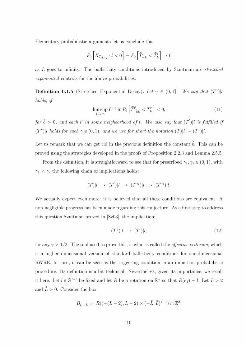
Elementary probabilistic arguments let us conclude that

P0

”

XTAL,l¨ l ă 0

ı

“ P0

”

rT l´L ărT lL

ı

Ñ 0

as L goes to infinity. The ballisticity conditions introduced by Sznitman are stretched

exponential controls for the above probabilities.

Definition 0.1.5 (Stretched Exponential Decay). Let γ P p0, 1s. We say that pT γq|l

holds, if

lim supLÑ8

L´γ lnP0

”

rT l1

´rbLă T l

1

L

ı

ă 0, (11)

for rb ą 0, and each l1 in some neighborhood of l. We also say that pT1

q|l is fulfilled if

pT γq|l holds for each γ P p0, 1q, and we use for short the notation pT q|l :“ pT 1q|l.

Let us remark that we can get rid in the previous definition the constant rb. This can be

proved using the strategies developed in the proofs of Proposition 2.2.3 and Lemma 2.5.5.

From the definition, it is straightforward to see that for prescribed γ1, γ2 P p0, 1q, with

γ1 ă γ2 the following chain of implications holds:

pT q|l Ñ pT1

q|l Ñ pT γ2q|l Ñ pT γ1q|l.

We actually expect even more: it is believed that all these conditions are equivalent. A

non-negligible progress has been made regarding this conjecture. As a first step to address

this question Sznitman proved in [Sz03], the implication:

pT γq|l Ñ pT1

q|l, (12)

for any γ ą 12. The tool used to prove this, is what is called the effective criterion, which

is a higher dimensional version of standard ballisticity conditions for one-dimensional

RWRE. In turn, it can be seen as the triggering condition in an induction probabilistic

procedure. Its definition is a bit technical. Nevertheless, given its importance, we recall

it here. Let l P Sd´1 be fixed and let R be a rotation on Rd so that Rpe1q “ l. Let L ą 2

and L ą 0. Consider the box

Bl,L,L :“ Rpp´pL´ 2q, L` 2q ˆ p´L, Lqd´1q X Zd,

10

with the positive part of its boundary B`Bl,L,L defined via

B`Bl,L,L :“ BB X tx P Zd, x ¨ l ě L` 2, |Rpeiq ¨ x| ă L, i ě 2u.

We also attach three random variables p, q and ρ to this box , defined by the following

relations

qpωq :“ P0,ωrXTBl,L,L

R B`Bl,L,Ls “ 1´ ppωq

along with

ρ “qpωq

ppωq

We are ready to define the effective criterion as follows:

Definition 0.1.6 (Effective Criterion). Let l P Sd. Then the effective criterion with

respect to l is satisfied if for some L ą c2, L P r3?d, L3q and a P r0, 1s the requirement

#

c3

ˆ

ln

ˆ

1

κ

˙˙3pd´1q

Ld´1L3d´2Erρas

+

ă 1,

Here, c2 and c3 are dimension dependent constants.

Notice that the effective criterion shares some similarities with the Solomon criterion

Erρs ă 1 which ensures ballistic regime, as it can be seen from (0.0.2). We can be more

precise yet with the statement of the equivalence in (12). Indeed the following theorem

due to Sznitman uses the effective criterion as a pivotal condition.

Theorem 0.1.7 (Sznitman). The following statements are equivalent:

• Effective Criterion with respect to l.

• pT 1q|l .

• pT γq|l for 1 ą γ ą 12.

The proof of this theorem can be found in [Sz03]. Furthermore, in [BDR14] N. Berger,

A. Drewitz and A. F. Ramırez proved the equivalence between this criterion and a poly-

nomial decay of the probability entering in (11). Specifically, the polynomial condition in

11

a non-effective form is the following requirement: let M ą 0. The polynomial condition

pP ˚qM |l is satisfied if:

limLÑ8

L´MP0

”

rT l1

´rbLă T l

1

L

ı

“ 0

for each l1 in some neighborhood of l and rb ą 0. One has the following:

Theorem 0.1.8 (Berger, Drewitz and Ramırez). Suppose that pP ˚qM |l is satisfied for

some M ą 15d` 5. Then the Effective Criterion with respect to l is satisfied.

Let us remark that actually in [BDR14], an effective version of the above polynomial

condition on boxes was introduced. This means that it is a condition that in principle

can be verified looking at the environment in large but finite boxes. The authors in this

article also proved that the Effective Criterion of Sznitman is implied by their polynomial

effective condition. Thus, using this polynomial effective condition one can avoid the use

of the Effective Criterion to check ballisticity. On the other hand, using the equivalence

between the Effective Criterion in direction l and pT1

q|l we conclude that

Theorem 0.1.9 (Berger, Drewitz, Ramırez and Sznitman). The following conditions are

equivalent:

• pT 1q|l.

• pT γq|l for 1 ą γ ą 0.

• pP ˚qM |l for M ą 15d` 5.

• Effective Criterion with respect to l.

As it was tacitly induced in the name given to pT γq|l for γ P p0, 1s, under these

conditions ballistic behavior is fulfilled. More precisely, combining (0.1.9) and Theorem

3.3 of [Sz03] we have that all the conditions in Theorem 0.1.9 satisfy :

P0 ´ a.s.,Xn

nÑ v “

E0rXτ1 | D “ 8s

E0rτ1 | D “ 8s,

12

with v ¨ l ą 0. Furthermore the random variable τ1 has finite moments of any arbitrary

order, and

Bn¨ :“

Xr¨ ns ´ r¨ nsv?nt

converges in law on Skorohod space DpR`, Rdq under P0 to the law of a non-degenerate

Brownian Motion with matrix covariance given by

A “E0rpXτ1 ´ τ1vq

tpXτ1 ´ τ1vq | D “ 8s

E0rτ1 | D “ 8s.

It is then possible to show that the ballisticity conditions in direction l imply that

P0- a.s.,T luuÑ pv ¨ lq´1 as uÑ 8.

Thus the walk escapes through direction l as if it had a local drift in direction l. Therefore

the walk behavior is in concordance with the informal idea of what is meant by ballistic

behavior. Besides seeing the effective criterion as a tool so as to get higher functional

controls from lower ones on the walk exit probability by the unlikely side from slabs, we

would like to mention that Sznitman in [Sz04] has found ballistic random walk exam-

ples satisfying pT1

q|l where the Kalikow’s condition breaks down. As a result Kalikow’s

condition is not the weakest condition which ensures a ballistic behavior. Furthermore,

it is conjectured that pT1

q|l is equivalent to ballisticity in direction l, which implies that

Conjecture 0.0.3 can be rephrased as:

pT1

q|l Ø the walk is transient in direction l.

This ends our survey about ballisticity conditions in i.i.d. random environments.

0.2 Previous results for random walks in cone mixing

random environments

In this section we would like to mention some results for random walks in random envi-

ronments which are not i.i.d. The main result of Chapter 2 of this thesis is formulated in

a framework of random walks in random environments which satisfy a mixing condition

13

discussed in [CZ01], and called cone mixing condition. In [CZ01] it is proven that random

walks in random environments satisfying a form of Kalikow’s condition, cone mixing, and

some important additional assumptions, are ballistic. A similar result was obtained by

Rassoul-Agha in [RA03], where he assumes also Kalikow’s condition and a mixing con-

dition stronger that cone mixing called Dobrushin-Shlosman strong mixing assumption.

Let us now describe these results.

We first describe the main result in [CZ01], which ensures ballisticity under some

conditions on the environment. Since mixing on cones is strictly weaker than the i.i.d.

condition, it will not be surprising that we will have to strengthen the ballisticity condi-

tions in order to ensure ballistic behavior. Even more, we will have to define approximate

regeneration times, since the standard definition of them in the i.i.d. context does not

work. For large fixed integer L we define τ1pLq as the first time that the walk reaches

a record level in direction l at time τ1pLq ´ L, and such in the following L steps after

this time, the walk does successive steps in the direction l. Further, after time τ1pLq, the

walk never exits the cone CpXn, l, αq again. This random time is much larger than the

standard regeneration time used in the i.i.d. case. In fact, it can be shown that both

τ1pLq and Xτ1pLq are of order κ´L as LÑ 8. We also need to switch the stopping time D

defined in (10) by D1, which is essentially defined as the first exit time of the set Cp0, l, αq.

We now need a suitable extension of the Kalikow’s condition. For V a finite, connected

subset of Zd, with 0 P V , we let

FV c “ σtωpz, ¨q : z R V u.

The Kalikow’s random walk tXn : n ě 0u with state space V Y BV and starting from

y P V Y BV is defined by the transition probabilities

pPV px, x` eq :“

$

&

%

E0rřTV cn“0 1tXn“xuωpx,eq|FV c s

E0rřTV cn“0 1tXn“xu|FV c s

, for x P V and e P U

1 for x P BV and e “ 0.

We denote by Py,V the law of this random walk and by Ey,V the corresponding expectation.

The following extension of the Kalikow’s condition was introduced in [CZ01].

Definition 0.2.1 (Kalikow’s conditional condition). Let δ ą 0. We say that Kalikow’s

14

conditional condition with respect to the direction l is satisfied if there exists a positive

constant δ such that

infV :xPV

pdV pxq ¨ l ě δ,

where

pdV pxq :“ pEx,V rX1 ´X0s “ÿ

|e|“1

e pPV px, x` eq

denotes the drift of Kalikow’s random walk at x, and the infimum runs over all finite

connected subset V of Zd such that 0 P V . We denote this condition by pKCqδ.

Finally, we set:

F0,L :“ σ

"

ωpy, ¨q; y ¨ l ď ´L

|u|1|u|2

*

.

The main result in [CZ01] is the following.

Theorem 0.2.2 (Comets and Zeitouni). Consider a random walk in a random envi-

ronment satisfying Kalikow’s conditional condition pKCqδ, the cone mixing condition

pCMqα,φ|l and the ellipticity assumption pUEq|l. Assume also that there exists a pos-

itive function MpLq depending just on L such that for some ϑ ą 1 one has that

PrE0rpκLτ1q

ϑ| F0,Ls ąM s “ 0 (13)

and satisfying limLÑ8MpLq1ϑ1 φ1pLq

1α “ 0, where ϑ1 :“ ϑpϑ´ 1q along with

φ1 :“2φ

P0rD1 “ 8s ´ φ.

Then there exists a deterministic v P Rd ´ t0u such that P0- a.s.

limXn

nÑ v,

with v ¨ l ą 0.

The integrability condition (13) is essentially required in order to establish a law of large

numbers along a regeneration time sequence which is not i.i.d. In the i.i.d. case, and

15

under the polynomial ballisticity condition pP ˚qM |l when M ě 15d` 5 (c.f. Theorem), it

is satisfied (as a matter of fact any moment of τ1 is finite). Nevertheless, the integrability

condition (13) is quite unsatisfactory, since it is in general difficult to check wether a

given random environments satisfies it or not. As a mater of fact, in [CZ01], a non-trivial

example which satisfies (13) is given, but the argument presented there is not completely

clear.

On the other hand, Rassoul-Agha in [RA03], under a mixing condition called Dobrushin-

Shlosman strong mixing assumption (see [CZ01] or [RA03]) has proved ballistic behav-

ior by means of a clever application of the environment as seen from the random walk

technique. It is important to stand out that Rassoul-Agha has only assumed the usual

Kalikow’s condition. However it was mentioned above that Kalikow’s condition is strictly

stronger than condition pT 1q [Sz04].

On the other hand, further important results can be found for instance in [CZ02],

[RA05] and [G14]. In [CZ02] the authors proved suitable versions of the central limit

theorem for the random walk in two kinds of environments: cone mixing and Dobrushing

strong mixing. In [RA05], the author has investigated conditional versions of the strong

law of large numbers. There it is proved that under an elliptic assumption and Dobrushin-

Shlosman strong mixing condition on the environment a weak version of the strong law

of large number is satisfied. Finally, Guo in [G14] under similar assumptions gave an

alternative proof of the result in [RA05] by means of regeneration arguments (instead

of the theoretical tool used by Rassoul-Agha: the environment as seen from the random

walk) and proved that there is at most one nonzero limit velocity when d ě 5 (originally

proved in the i.i.d. case by Berger in [Be08]).

In conclusion, in both of the articles [CZ01] and [RA03] some version of Kalikow’s

condition is assumed. Furthermore, neither these works nor the ones mentioned in the last

paragraph, discuss possible adaptations of weaker ballisticity conditions like conditions

pT q, pT 1q or pP qM , to environments which are not necessarily i.i.d., even less so asymptotic

results under these kind of conditions. One of the objectives of this thesis, developed in

Chapter 2, is to give a first indication about how should these ballisticity conditions be

defined for cone mixing environments.

16

0.3 A brief explanation of the Thesis Results

In this section we will describe the results of each chapter.

0.3.1 Main Result for i.i.d. Random Environments

A problem left untouched in the quoted results of Section 0.1.2 is the following question:

Conjecture 0.3.1. For a random walk in a uniformly elliptic i.i.d. environment, condi-

tion pT1

q|l is equivalent to pT q|l.

Chapter 1 of this thesis addresses this question. The main result of Chapter 1 shows

that condition pT 1q|l implies an almost exponential decay for the exit probability of the

random walk through the back side of slabs (which is very close to pT q|l). Specifically, for

a given direction l and L ą 0 we denote by Sl,L the strip tx P Rd : |x ¨ l| ď Lu and by Al,L

the event that the walk starting from 0 exits Sl,L through the side of Sl,L where x ¨ l ă 0.

Now, for a given direction l and function γ : r0,8q Ñ r0, 1s we say that the condition

pT qγpLq|l is satisfied if for all directions l1 in a neighborhood of l there is a constant c ą 0

such that asymptotically as LÑ 8 it is true that

P0rAl1,Ls “ e´cLγpLq`opLγpLqq.

It is straightforward to check that by definition, condition pT q|l is equivalent to

pT qγ1pLq|l with

γ1pLq “ 1´ C1

logpLq,

for any C ą 0. On the other hand, in [Sz03] Sznitman proved that pT 1q|l implies pT qγ2pLq|l

with

γ2pLq “ 1´ Clog

12 pLq

logpLq.

In Chapter 1 of this thesis, we prove that pT 1q|l implies pT qγ3pLq|l with

γ3pLq “ 1´ rClognpLqpLq

logpLq, (14)

17

where rC is a positive constant and npLq a function with values in the positive integers

that has limit infinity as L Ñ 8. logk denotes the function logarithm composed k ´ 1

times with itself; i.e., logkpxq “

khkkkkkkkkkkkkkikkkkkkkkkkkkkj

log ˝ log ˝ log ˝ . . . ˝ logpxq. In spite that this result seems

to be close to answering affirmatively Conjecture 0.3.1, it does not. Indeed, the function

npLq of (14) is such that

limLÑ8

lognpLqpLq “ 8.

The proof of this result relies on renormalization arguments which have the Effective

Criterion as a seed condition.

0.3.2 Main Result for cone mixing random environments

Chapter 2 of this thesis is concerned with random walks in cone mixing random envi-

ronments. The main result is the proof that under a non-effective polynomial ballisticity

condition, these random walks have an asymptotic direction (see ??). In what follows we

will define this version of the polynomial ballisticity ccondition. Given L,L1 ą 0, x P Zd,

we define the boxes

BL,L1,lp0q :“ R´

p´L,Lq ˆ p´L1, L1qd´1

¯

X Zd,

where R is a rotation on Rd such that Rpe1q “ l. Define the positive boundary of BL,L1,lpxq,

denoted by B`BL,L1,lp0q, as

B`BL,L1,lp0q :“ BBL,L1,lp0q X tz : z ¨ l ě Lu,

Define also the half-space

Hx,l :“ ty P Zd : y ¨ l ă x ¨ lu,

and the corresponding σ-algebra of the environment on that half-space

Hx,l :“ σpωpyq : y P Hx,lq.

Now, for M ě 1, we say that the non-effective polynomial condition pPCqM,c|l is satisfied

if there exists some c ą 0 so that for y P H0,l one has that

18

limLÑ8

LM supP0

”

XTBL,cL,l p0qR B

`BL,cL,lp0q, TBL,cL,lp0q ă THy,l |Hy,l

ı

“ 0, (15)

where the supremum is taken over all possible environments to the left of y¨l. We prove the

existence of an asymptotic direction for random walks in random environment satisfying

the condition pCMqα,φ|l under the assumptions pPCqM,c|l and pUEq|l, where the positive

constants M, c and α satisfy the constraints:

M ą 6d and 0 ă α ď mint1

9,

1

2c` 1u (16)

We will prove that the non-effective polynomial condition is weaker than the conditional

version of Kalikow’s condition introduced in [CZ01]. We would like to sketch the general

strategy behind the proof of this result. As a first step we need to prove that:

P0rD1“ 8s ą 0. (17)

Let us remark that we do not need a conditional version of the ballisticity assumption to

prove this. To prove the claim (17), we have used renormalization type methods, so as

to apply the polynomial condition. Specifically, using the assumption pUEq|l we can and

we do assume that the walk starting from 0 goes on a large distance through direction l

up to a fixed point z with positive annealed probability, and starting from that point one

can show that with a high probability the walk remains forever inside of each half-space:

H˘i :“ ty : py ´ zq ¨ l˘i ě 0u, for i P r2, ds. Finally the result follows from the definition

of the cone. We refer to the proof of Proposition 2.4.1 in Chapter 2 for the precise

argument. As a second step, we proved a strong integrability result of the regeneration

position Xτ1pLq. Roughly speaking, we have proved that the conditional expectation of

the second moment of the regeneration position is finite. These two steps are the core

of the proof. Indeed using for instance similar arguments as the ones given in [CZ01] we

can obtain the asymptotic direction pv. The main issue to integrate the second moment of

the random variable κLXτ1pLq was to connect i.i.d. methods with the cone mixing model.

We connect them by identifying how close (or far) the old τ1 is from the new τ1pLq. The

precise statement of the required integrability condition and its proof are given in Section

2.5 of Chapter 2.

19

On the other hand, the simpler Simenhaus’s approach [Si07] does not work in cone

mixing environment at least if we identify the random variable τ1 with τ1pLq. The ar-

gument of [Si07] makes a strong use of i.i.d. assumption on the environment. The

i.i.d. structure of the environment space is explicitly required in the renewal theorem

to prove Zerner’s formula (c.f. Lemma 2 in [Si07]) and in order to prove that the sequence

pZkq :“ supně0 |Xn^τk`1´Xτk | is such that Znn converges P0-a.s. to 0 as n Ñ 8. The

first argument breaks down in the cone-mixing case, mainly because one cannot apply

the renewal theorem without assuming some kind of strong integrability condition for the

regeneration position. Furthermore, as an example to understand possible pathologies in

the behavior of a random walk in a cone mixing environment, we provided an example of

a random walk defined in a cone mixing environment which is directionally transient but

not ballistic, showing that we cannot expect the ballisticity conjecture 0.0.3 to be valid

outside of the i.i.d. setting. Consequently one could ask the following: what would be

the kind of natural conditions which ensure that the random walk satisfies a strong law of

large numbers with a non-vanishing limit velocity in this framework? We expect that the

machinery developed in Chapter 2 could serve in a future work to prove ballistic behavior

under a ballisticity condition similar to condition pT 1q.

The two results are a joint work with Alejandro Ramırez.

20

Chapter 1

Almost exponential decay for the

exit probability from slabs of

ballistic RWRE

1.1 Introduction

The relationship between directional transience and ballisticity for random walks in ran-

dom environment is one of the most challenging open questions within the field of random

media. In the case of random walks in an i.i.d. random environment, several ballisticity

conditions have been introduced which quantify the exit probability of the random walk

through a given side of a slab as its width L grows, with the objective of understanding

the above relation. Examples of these ballisticity conditions include Sznitman’s pT 1q and

pT q conditions [Sz02, Sz03]: given a slab of width L orthogonal to l, condition pT 1q in

direction l is the requirement that the annealed exit probability of the walk through the

side of the slab in the half-space tx : x ¨ l ă 0u, decays faster than e´CLγ

for all γ P p0, 1q

and some constant C ą 0, while condition pT q in direction l is the requirement that the

decay is exponential e´CL. It is believed that condition pT 1q, is equivalent to condition

pT q. In this chapter we prove that condition pT 1q implies an almost exponential decay

(see Theorem 1.1.2 for the precise meaning of this statement) of the corresponding exit

probabilities. Our proof relies on a recursive renormalization scheme, where the a careful

21

choice of fastly growing scales enables us to obtain the result. We use the equivalence

between condition pT 1q [Sz03] and the d ě 2 dimensional version of Solomon’s criterion

[So75], known as the effective criterion [Sz03].

Let us introduce the random walk in random environment model. For x P Zd denote

its euclidean norm by |x|2. Let V :“ te P Zd : |e|2 “ 1u be the set of canonical vectors.

Introduce the set P whose elements are 2d´vectors ppeqe PZd, |e|“1 such that

ppeq ě 0, for all e P V ,ÿ

e PZd, |e|“1

ppeq “ 1.

We define an environment ω :“ tωpxq : x P Zdu as an element of Ω :“ PZd , where for each

x P Zd, ωpxq “ tωpx, eq : e P V u P P . Consider a probability measure P on Ω endowed

with its canonical product σ-algebra, so that an environment is now a random variable

such that the coordinates ωpxq are i.i.d. under P. The random walk in the random

environment ω starting from x P Zd is the canonical Markov Chain tXn : n ě 0u on pZdqN

with quenched law Px,ω starting from x, defined by the transition probabilities for each

e P Zd with |e| “ 1 by

Px,ωrXn`1 “ Xn ` e|X0, . . . , Xns “ ωpXn, eq

and

Px,ωrX0 “ xs “ 1.

The averaged or annealed law, Px, is defined as the semi-direct product measure

Px “ Pˆ Px,ω

on Ωˆ pZdqN. Whenever there is a κ ą 0 such that

infe,xωpx, eq ě κ P´ a.s.

we will say that the law P of the environment is uniformly elliptic.

For the statement of the result, we need some further definitions. For each subset

A Ă Zd we define the first exit time of the random walk from A as

22

TA :“ inftn ě 0 : Xn R Au.

Fix a vector l P Sd´1 and u P R then define the half-spaces H´u,l :“ tx P Zd : x ¨ l ă uu,

H`u,l :“ tx P Zd : x ¨ l ą uu,

T lu :“ TH´u,l“ inftn ě 0, Xn ¨ l ě uu

and

T lu :“ TH`u,l“ inftn ě 0, Xn ¨ l ď uu.

For γ P p0, 1s, we say that condition pT qγ|l holds with respect to direction l P Sd´1, if

lim supLÑ8

L´γ log P0rTl1

´L ă T l1

L s ă 0,

for all l1 in some neighborhood of l. Furthermore, we define pT 1q|l as the requirement that

condition pT qγ|l is satisfied for all γ P p0, 1q and condition pT q|l as the requirement that

pT q1|l is satisfied. In [Sz03], Sznitman proved that when d ě 2 for every γ P p0.5, 1q, pT qγ|l

is equivalent to pT 1q|l. This equivalence was improved in [DR11] and [DR12] culminating

with the work of Berger, Drewitz and Ramırez who in [BDR14] showed that for any

γ P p0, 1q, condition pT qγ|l implies pT 1q|l. As a matter of fact, in [BDR14], an effective

ballisticity condition, which requires polynomial decay was introduced. To define this

condition, consider L, L ą 0 and l P Sd´1 and the box

Bl,L,L :“ R´

p´L,Lq ˆ p´L, Lqd´1¯

X Zd,

where R is a rotation defined by

Rpe1q “ l. (1.1)

Given M ě 1 and L ě 2, we say that the polynomial condition pP qM in direction l (also

denoted by pP qM |l) is satisfied on a box of size L if there exists and L ď 70L3 such that

P0

”

XTBl,L,L

¨ l ă Lı

ď1

LM.

23

Berger, Drewitz and Ramırez proved in [BDR14] that there exists a constant c0 such that

whenever M ě 15d ` 5, the polynomial condition pP qM |l on a box of size L ě c0 is

equivalent to condition pT 1q|l (see also Lemma 3.1 of [CR14]). On the other hand, the

following is still open.

Conjecture 1.1.1. Consider a random walk in a uniformly elliptic random environment

in dimension d ě 2 and l P Sd´1. Then, condition pT q|l is equivalent to pT 1q|l.

To quantify how far are we presently from proving Conjecture 1.1.1, we will introduce

now a family of intermediate conditions between conditions pT 1q and pT q. Let γpLq :

r0,8q Ñ r0, 1s, with limLÑ8 γpLq “ 1. Let l P Sd. We say that condition pT qγpLq|l is

satisfied if

lim supLÑ8

L´γpLq logP0rTl1

´L ă T l1

L s ă 0, (1.2)

for l1 in a neighborhood of l. We will call γpLq the effective parameter of condition pT qγpLq.

Note that condition pT q is actually equivalent to pT qγpLq with an effective parameter given

by

γpLq “ 1´C

logL, (1.3)

for any constant C ě 0.

In 2002 Sznitman [Sz03] was able to prove that pT 1q implies pT qγpLq with effective

parameter

γpLq “ 1´C

logL

a

logL, (1.4)

for some constant C ą 0.

In this chapter, we are able to show that condition pT 1q implies condition pT qγpLq with

an effective parameter γpLq which is closer to the effective parameter for condition pT q

given by (1.3). This is the first result since the introduction of condition pT 1q by Sznitman

in 2002, which would give an indication that Conjecture 1.1.1 is true. To state it, let us

introduce some notations. Throughout, for each n ě 1, we will use the standard notation

24

nhkkkkkkikkkkkkj

log ˝ ¨ ¨ ¨ ˝ log x,

for the composition of the logarithm function n times with itself, for all x in its domain,

where the n superscript means that the composition is performed n times.

Theorem 1.1.2. Let d ě 2, l P Sd´1 and M ě 15d ` 5. Assume that condition pP qM |l

is satisfied on a box of size L ě c0. Then there exists a constant C ą 0 and a function

npLq : r0,8q Ñ N satisfying limLÑ8 npLq “ 8, such that condition pT qγpLq|l, c.f. (1.2),

is satisfied with an effective parameter γpLq given by

γpLq “ 1´C

logL

npLqhkkkkkkikkkkkkj

log ˝ ¨ ¨ ¨ ˝ logL. (1.5)

Remark 1.1.3. Note that the decay given by the effective parameter (1.5) of Theorem

1.1.2 is equivalent to the decay

lim supLÑ8

npLq´1hkkkkkkikkkkkkj

log ˝ ¨ ¨ ¨ ˝ logL

LlogP0rT

l1

´L ă T l1

L s ă 0,

for l1 in a neighborhood of l.

Let us remark that a priori, even if npLq Ñ 8 as L Ñ 8, it might happen that the

composition of the logarithm npLq time is bounded. Nevertheless, in the case of Theorem

1.1.2, it turns out that

limLÑ8

npLqhkkkkkkikkkkkkj

log ˝ ¨ ¨ ¨ ˝ logL “ 8.

Theorem 1.1.2 will be proven in the next section, but some remarks are in order. The

strategy followed in the proof, roughly speaking, is to improve the iterative procedure

used by Sznitman in [Sz02], to prove pT qγpLq with γpLq given by (1.4), through the so

called effective criterion introduced by Sznitman in [Sz03]. The iterative procedure used

in [Sz03], in spirit is a renormalization argument, where the idea is to control the exit

probability of the walk recursively from an initial scale L0 to the final size of the slab

25

L ą L0 passing through a sequence of intermediate scales L0 ă L1 ă . . . ă Lk “ L.

To go from scale L0 to scale L1, a slab of width L1 is subdivided into overlapping slabs

of width L0, and the walk is looked at its exit times from successive slabs of width L0.

Essentially, at these times the walk looks like a one dimensional random walk in random

environment, for which one can control its exit probabilities through the expected value

of ρ, where ρ is close to the quotient between the probability to exit a slab of width L0

through its left side and the probability to exit it through its right side. Here, a triggering

assumption is needed, which in our case is the effective criterion of Sznitman [Sz02] (the

effective criterion is implied by the polynomial condition introduced by Berger, Drewitz

and Ramırez in [BDR14]). This first step is the content of Proposition 2.1. A similar

strategy is then used to pass from scale Lk to scale Lk`1 for k ě 1 (see Lemma 2.2).

Nevertheless, reducing the movement of the random walk to a one dimensional walk,

has a cost, which is a polynomial factor appearing in the recursion relations, and which

somehow is the reason why one cannot go from the initial scale L0 directly to L in one

step. In this chapter, we modify Sznitman’s argument, choosing a sequence of scales where

Lk`1 is much larger than Lk compared to Sznitman’s approach, allowing us to work with

a smaller number of intermediate steps in the recursion relation. The use of this new

sequence of scales, produces at some points important difficulties in the proof which have

to be properly handled.

1.2 Proof of Theorem 1.1.2

Throughout the rest of this section, we prove Theorem 1.1.2. Firstly, in subsection 1.2.1,

we will introduce the basic notation which will be needed to implement the renormalization

scheme, and we will recall a basic result of Sznitman which provides a bound for quantities

involving the exit probability through the unlikely side of boxes which are inspired in

techniques for used for one-dimensional random walks in random environment. In the

second subsection, we will introduce a growth condition which will limit the maximal way

in which the scales on the renormalization scheme can grow, while still giving a useful

recurrence. In the third subsection we will choose an adequate sequence of scales satisfying

the condition of subsection 1.2.2, and for which one can make computations. Finally, in

26

subsection 1.2.4, Theorem 1.1.2 will be proven using the scales constructed in subsection

1.2.3 through the use of the effective criterion [Sz02].

1.2.1 Preliminaries and notation

The proof of Theorem 1.1.2 will follow the renormalization method used by Sznitman to

prove Proposition 2.3 of [Sz02]. The idea is to use a renormalization procedure which

somehow mimics a computation for a one-dimensional random walk in random environ-

ment, where one goes from one scale to the next (larger) one through formulas where the

exit probabilities of the random walk through slabs at the smaller scales are involved.

Following Sznitman we introduce boxes transversal to direction l, which are specified

in terms of B “ pR,L, L1, Lq, where L,L1, L are positive numbers and R is the rotation

defined in (2.3). The box attached to B, is

B :“ Rpp´L,L1q ˆ p´L, Lqd´1q X Zd

and the positive part of its boundary is defined as

B`B :“ BB X tx P Zd, x ¨ l ě L1, |Rpeiq ¨ x| ă L, i ě 2u.

We can now define the following random variable depending on a given specification B,

analogous to the quotient in dimension d “ 1 between the probability to jump to the left

and the probability to jump to the right [SW69, So75], for ω P Ω as

ρBpωq :“qBpωq

pBpωq,

where

qBpωq :“ P0,ωrXTB R B`Bs “: 1´ pBpωq.

The first step in the renormalization procedure will be to control the moments of ρB at

the two first scales. To this end, consider positive numbers

3?d ă L0 ă L1, 3

?d ă L0 ă L1

along with the box-specifications

27

B0 :“ pR,L0 ´ 1, L0 ` 1, L0q

and

B1 :“ pR,L1 ´ 1, L1 ` 1, L1q.

It is convenient to introduce now the notation

q0 :“ qB0 , p0 :“ pB0 , q1 :“ qB1 , p1 :“ pB1 ,

and

ρ0 :“ ρB0 , ρ1 :“ ρB1 . (1.6)

Let also

N0 :“L1

L0

and N0 :“L1

L0

.

We will also need to introduce the constant

c1pdq “ c1 :“?d.

Note that for each pair of points x, y P Zd, there exists a nearest neighbor path joining

them which has less than c1|x´ y|2 steps.

Let us now recall the following Proposition of Sznitman [Sz03].

Proposition 1.2.1. There exist c2pdq ą 3?d, c3pdq, c4pdq ą 1, such that when N0 ě

3, L0 ě c2, L1 ě 48N0L0, for each a P p0, 1s one has that

E”

ρa21

ı

ď c3

#

κ´10c1L1

´

c4Ld´21

L31

L20L0Erq0s

¯

L112N0L0

`ř

0ďmďN0`1

´

c4Ld´11 Erρa0s

¯

rN0s`m´12

+

. (1.7)

28

1.2.2 The maximal growth condition on scales

We next recursively iterate inequality (1.7) at different scales which will increase as fast as

possible, in the sense that a certain induction condition should enable us to push forward

the recursion.

We next recursively iterate inequality (1.7) at different scales which will increase as

fast as possible, in the sense that a certain induction hypothesis should enable us to push

forward the recursion. Let

v :“ 8, α :“ 240

and introduce two sequences of scales Lk, Lk k ě 0, such that

L0 ě c2 , 3?d ă L0 ď L3

0 (1.8)

and for k ě 0

Nk ě 7, Lk`1 “ NkLk, Lk`1 “ N3k Lk, (1.9)

as well as box-specifications

Bk :“ pR,Lk ´ 1, Lk ` 1, Lkq.

Note that

Lk`1 “

ˆ

LkL0

˙3

L0. (1.10)

Introduce also the notation for the respective attached random variables

ρk :“ ρBk .

Throughout, we will adopt the notation

u0 :“3pd´ 1q

L0 log 1κ

, (1.11)

and for k ě 1,

29

uk :“u0

vk. (1.12)

We also let

c5 :“ 2c3c4.

Condition pGq. We say that the scales Lk, Nk, k ě 0 satisfy condition pGq if

ukNk ě αc1 for k ě 0, (1.13)

and if

c5N3pd´1qk`1 L3d´1

k`1 κuk`1Lk`1 ď 1 for k ě 0. (1.14)

Let us now state the following lemma which generalizes Lemma 2.2 of Sznitman

([Sz03]), for scales satisfying condition pGq. For completeness we include its proof.

Lemma 1.2.2. Consider scales Lk, Nk, k ě 0, such that condition pGq is satisfied. Then,

whenever L0 ě c2, 3?d ď L0 ď L3

0, and a0 P p0, 1s, we have that

ϕ0 :“ c4Ld´11 L0Erρa00 s ď κu0L0 . (1.15)

then for all k ě 0,

ϕk :“ c4Ld´1k`1LkErρ

akk s ď κukLk . (1.16)

with

ak “ a02´k, uk “ u0v´k.

Proof. As in the proof of Lemma 2.2 of [Sz02], we can conclude by Proposition 1.2.1 that

if L0 ě c2 (note that by the choice of Nk in (1.9), the other conditions of Proposition 1.2.1

are satisfied) we have that for k ě 0,

30

ϕk`1 ď c3c4Ld´1k`2Lk`1

#

κ´10c1Lk`1ϕN2k

12k `

ÿ

0ďmďNk`1

ϕrNks`m´1

2k

+

. (1.17)

We will now prove inequality (1.16) by induction on k using inequality (1.17). Since

inequality (1.15) is identical to inequality (1.16) with k “ 0, the induction hypothesis is

satisfied for k “ 0. We assume now that it is true for k ą 0, along with inequality (1.13)

of assumption pGq and conclude that

κ´10c1Lk`1ϕN2k

24k ď κ´10c1Lk`1κN

2kLkuk24 ď 1. (1.18)

Therefore, using (1.18) and the fact that rNks ´ 1 ě Nk2

because Nk ě 7 we see that

ϕk`1 ď c3c4Ld´1k`2Lk`1

#

ϕN2k

24k ` Lk`1ϕ

Nk4k

+

ď c5Ld´1k`2L

2k`1ϕ

Nk8k ϕ

Nk8k , (1.19)

where we recall that c5 “ 2c3c4. Now, by the induction hypothesis (1.16) we see that

ϕNk8k ď κuk`1Lk`1 .

Substituting this into (1.19), we see that it is enough now to show that

c5Ld´1k`2L

2k`1ϕ

Nk8k ď 1.

But this is true, by (1.14) of condition pGq, the induction hypothesis and the inequality

Lk`1 ď L3k`1 for k ě 0 which follows by induction starting from (1.8). Indeed, using these

facts,

c5Ld´1k`2L

2k`1ϕ

Nk8k ď c5N

3pd´1qk`1 L3d´1

k`1 κuk`1Lk`1 ď 1,

which ends the proof.

31

1.2.3 An adequate choice of fast-growing scales

We will now construct a sequence of scales tLk : k ě 0u which satisfy condition pGq,

and for which Lemma 1.2.2 will eventually imply Theorem 1.1.2. This is not the fastest

possible growing sequence of scales, but somehow it captures the best possible choice of

γpLq.

Let tfk : k ě 1u be a sequence of functions from r0,8q to r0,8q defined recursively as

f0pxq :“ 1,

f1pxq :“ vx

and for k ě 1,

fk`1pxq :“ fk ˝ f1pxq.

Let now, for k ě 0,

Nk :“αc1

u0

fr k`22 s

`“

k`12

‰˘

fr k`12 s

`“

k2

‰˘ . (1.20)

According to display (1.9), we have the following formula valid for k ě 0,

Lk`1 “ fr k`22 s

ˆ„

k ` 1

2

˙ˆ

αc1

u0

˙k`1

L0. (1.21)

Lemma 1.2.3. The condition

ukNk ě αc1 for k ě 0

(c.f. (1.13) of condition pGq) is equivalent to

fr k`22 s

`“

k`12

‰˘

fr k`12 s

`“

k2

‰˘

vkě 1 for k ě 0. (1.22)

Furthermore, the last relation is fulfilled.

32

Proof. Note that (1.22) can be easily verified for k “ 0, 1 and 2. Therefore it is enough to

prove inequality (1.22) for k ě 3. For this purpose, we will first show that for all positive

integers n, and a, b P r1,8q, we have that

fn pa` bq ě fnpaqfnpbq. (1.23)

To prove (1.23), suppose that

A :“ tn P N : fn pa` bq ă fnpaqfnpbq for some a, b ě 1u ‰ ∅.

Let m be the smallest element of A and remark that m is greater than 1. Also, note that

fm pa` bq ă fmpaqfmpbq

for some a, b ě 1. However, note that for a, b ě 1 one has that

va`b ě va ` vb.

Furthermore, for each k ě 0, the function fkp¨q is increasing. Therefore,

fm´1pvaqfm´1pv

bq “ fmpaqfmpbq

ą fmpa` bq “ fm´1pva`bq ě fm´1pv

a ` vbq.

This contradicts the minimality of m and hence A “ ∅ which proves (1.23). Back to

(1.22), note that

fr k`2

2 spr k`1

2 sq

fr k`1

2 spr k2 sqv

kě

fr k`2

2 spr k`1

2 s´1q

fr k`1

2 spr k2 sq

fr k`2

2 sp1q

vkě

fr k`2

2 sp1q

vkě 1,

where the first inequality was gotten using (1.23), the second one is a consequence of the

inequality

fr k`22 s

`“

k`12

‰

´ 1˘

fr k`12 s

`“

k2

‰˘ ě 1,

33

valid for k ě 3, and which can be proved in a straightforward fashion if we divide the

argument according to whether k is even or odd, and the last inequality comes from the

fact that

fr k`2

2s´1p1q ´ k ě 0 for k ě 3. (1.24)

Now, it is easy to verify inequality (1.24) when k “ 3 and k “ 4. Furthermore, the left

hand of (1.24) is increasing as a function of k ě 2 for k odd. Similarly, it is increasing

for k ě 2 for k even. We can therefore conclude, using induction that (1.24) is satisfied.

This completes the proof of (1.22).

Using Lemma 1.2.3 we can now obtain the following important lemma which gives con-

ditions on the growth of a sequence of scale which ensure that pGq is satisfied.

Lemma 1.2.4. There exists a constant c6pdq such that when L0 ě c6, the scales tLk :

k ě 0u and tNk : k ě 0u defined by (1.21) and (1.20) satisfy condition pGq.

Proof. By Lemma 1.2.3 we know that (1.13) of condition pGq is satisfied. We therefore

just prove inequality (1.14) of condition pGq. We need to show that there exists a constant

cpd, κq, such that whenever L0 ě cpd, κq, for all k ě 0 one has that

c5N3pd´1qk`1 L3d´1

k`1 κuk`1Lk`1 ď 1. (1.25)

We will first show that there exists c7pd, κq “ c7pdq ą 0, such that whenever L0 ě c7, one

has that for k ě 0,

N3pd´1qk`1 κ

uk`1Lk`13 ď 1. (1.26)

Now (1.26) is equivalent to

3pd´ 1q logv

˜

αc1u0

fr k`3

2 spr k`2

2 sq

fr k`2

2 spr k`1

2 sq

¸

´

L0u0fr k`2

2 spr k`1

2 sq´

αc1vu0

¯k`1logvp

1κq

3ď 0.

34

Therefore, (1.26) is equivalent to the bound for k ě 0,

L0 ě

9pd´1qu0

logv

˜

αc1u0

fr k`3

2 spr k`2

2 sq

fr k`2

2 spr k`1

2 sq

¸

fr k`22 s

`“

k`12

‰˘

´

αc1vu0

¯k`1

logv`

1κ

˘

. (1.27)

Let us focus on right-hand side of inequality (1.27) . Note that it can be split as

9pd´1qu0

logv

´

αc1u0

¯

fr k`22 s

`“

k`12

‰˘

´

αc1vu0

¯k`1

logv`

1κ

˘

`

9pd´1qu0

logv

˜

fr k`3

2 spr k`2

2 sq

fr k`2

2 spr k`1

2 sq

¸

fr k`22 s

`“

k`12

‰˘

´

αc1vu0

¯k`1

logv`

1κ

˘

. (1.28)

Let us now try to find an upper bound for this expression independent on u0 (or equiv-

alently, on L0). By the definition of u0 (c.f. (1.11)) note that for k ě 0 and L0 ě3pd´1q

log 1κ

one has that,

1

u0

1´

αc1vu0

¯k`1“

1´

αc1vu0

¯k

1`

αc1v

˘ ď1

`

αc1v

˘k`1.

Substituting this into (1.28) we see that it is bounded from above by

9pd´ 1q logv

´

αc1u0

¯

fr k`22 s

`“

k`12

‰˘ `

αc1v

˘k`1logv

`

1κ

˘

`

9pd´ 1q logv

˜

fr k`3

2 spr k`2

2 sq

fr k`2

2 spr k`1

2 sq

¸

fr k`22 s

`“

k`12

‰˘ `

αc1v

˘k`1logv

`

1κ

˘

. (1.29)

Note that only the left-most term of (1.29) depends on L0. Choose a constant c8pd, κq “

c8pdq ą 1, such that if L0 ě c8

logv

ˆ

αc1

u0

˙

ď L0

logv`

1κ

˘

d´ 1. (1.30)

Then, when L0 ě c8, we see using the fact that the left-most term of (1.29) is a decreasing

function of k ě 0 and from inequality (1.30), that it can be bounded from above by

L09v

αc1

ď L072

240ďL0

3. (1.31)

35

Thus, whenever L0 ě c8, from (1.28), (1.29) and (1.31), we see that (1.27) is satisfied if

L0 ě3

2

9pd´ 1q logv

˜

fr k`3

2 spr k`2

2 sq

fr k`2

2 spr k`1

2 sq

¸

fr k`22 s

`“

k`12

‰˘ `

αc1v

˘k`1logv

`

1κ

˘

. (1.32)

Therefore, in order to prove (1.26) it is enough to show that the right hand side of

inequality (1.32) is bounded. To do this, it is enough to prove that the expression

logv

˜

fr k`3

2 spr k`2

2 sq

fr k`2

2 spr k`1

2 sq

¸

fr k`22 s

`“

k`12

‰˘

is bounded. Now,

logv

˜

fr k`3

2 spr k`2

2 sq

fr k`2

2 spr k`1

2 sq

¸

fr k`22 s

`“

k`12

‰˘ ď

logv

´

fr k`32 s

`“

k`22

‰˘

¯

fr k`22 s

`“

k`12

‰˘ . (1.33)

Let us now remark that if k is even, then“

k`32

‰

““

k`22

‰

and“

k`12

‰

““

k`22

‰

´1. Therefore,

in this case, the right-hand side of inequality (1.33) is smaller than

fr k`22 s´1

`“

k`22

‰˘

fr k`22 s

`“

k`22

‰

´ 1˘ “

fr k`22 s´1

`“

k`22

‰˘

fr k`22 s´1

´

vrk`22 s´1

¯ .

But, since for k fixed, the function fkp¨q is increasing, and since for k ě 0 we have that

vrk`22 s´1

ě

„

k ` 2

2

,

we see that the right-hand side of inequality (1.33) is bounded. Hence, for k even the

right-most term of (1.33) is bounded by a constant c9pd, κq “ c9pdq ą 0.

Suppose now that k is odd. Then“

k`32

‰

““

k`22

‰

` 1 and“

k`12

‰

““

k`22

‰

. Therefore, in

this case, the right-hand side of inequality (1.33) is equal to

fr k`22 s

`“

k`22

‰˘

fr k`22 s

`“

k`22

‰˘ “ 1,

so that we can conclude that the right-hand side of inequality (1.33) is bounded, and hence

that there is constant c10pd, κq “ c10pdq ą 0 which is an upper bound for the right-hand

36

side of inequality (1.27). We can hence conclude, taking c7pdq “ maxtc9pdq, c10pdqu, that

when L0 ě c7pdq, then (1.26) holds.

As a second step to prove (1.25), we will show that it is possible to find a positive

constant c11pd, κq “ c11pdq such that when L0 ě c11 one has that for all k ě 0,

L3d´1k`1 κ

uk`1Lk`13 ď 1. (1.34)

Inserting the definition (1.21) that defines Lk into this inequality, we see that it is enough

to prove that

p3d´ 1q logv pLk`1q ´

logv`

1κ

˘

u0

´

αc1u0v

¯k`1

fr k`22 s

`“

k`12

‰˘

L0

3ď 0. (1.35)

If we show that for all k ě 0, L0 ělogvpLk`1q3p3d´1q

logvp1κqu0

´

αc1u0v

¯k`1fr k`2

2 spr k`1

2 sq, we have a proof of (1.35).

But the right-hand side of this inequality can be written as

3p3d´ 1q logv

„

L0

´

αc1u0

¯k`1

logv`

1κ

˘

u0

´

αc1u0v

¯k`1

fr k`22 s

`“

k`12

‰˘

`

3p3d´ 1q logv

´

fr k`22 s

`“

k`12

‰˘

¯

fr k`22 s

`“

k`12

‰˘ .

We need to establish a control with respect to L0 in this expression. Only the first term

depends on L0 so we concentrate on the first term. Now, this term is decreasing with k.

Therefore, it is smaller than

3p3d´ 1q logv

”

L0

´

αc1u0

¯ı

logv`

1κ

˘ `

αc1v

˘ “

3p3d´ 1q logv

´

L20αc1 logp 1

κq

3pd´1q

¯

logv`

1κ

˘ `

αc1v

˘

From this last expression, it is clear that we can choose a constant c12pd, κq “ c12pdq ą 0

such that whenever L0 ě c12pdq one has that

3p3d´ 1q logv

„

L0

´

αc1u0

¯k`1

logv`

1κ

˘

u0

´

αc1u0v

¯k`1

fr k`22 s

`“

k`12

‰˘

ďL0

3. (1.36)

Therefore, if L0 ě c12pdq and if

L0 ě3

2

3p3d´ 1q logv

´

fr k`22 s

`“

k`12

‰˘

¯

fr k`22 s

`“

k`12

‰˘ , (1.37)

37

we would have (1.34), whenever we could prove that the right hand side of (1.37) is

bounded independently of k ě 0. This can be proven in analogy to the previous computa-

tions made to show that the right-hand side of (1.32) is bounded. We have thus established

the existence of a constant c11pdq such that (1.34) is satisfied whenever L0 ě c11pdq.

On the other hand it is obvious that there is a constant c13pdq, such that when L0 ě

c13pdq, for k ě 0,

c5κuk`1Lk`1

3 ď 1.

Finally, in order for inequality (1.14) of condition pGq to be fulfilled, it is enough to take

c6pdq :“ maxtc7pdq, c11pdq, c13pdqu.

1.2.4 The effective criterion implies Theorem 1.1.2

We continue now showing how Lemma 1.2.2 with the appropriate choice of scales, enables

us to use the effective criterion (see Theorem 2.4 of [Sz03] where it was introduced) to

prove the decay of Theorem 1.1.2. Let us define for x P Zd,

|x|K :“ maxt|x ¨Rpeiq| : 2 ď i ď du.

Also, define for each x P Zd, the canonical translation on the environments tx : Ω Ñ Ω as

txpωqpyq :“ ωpx` yq for y P Zd.

For the statement of the following proposition and its proof, we will use the shorthand

notation for each n,

logpnq8 pLq :“

nhkkkkkkkikkkkkkkj

log8 ˝ ¨ ¨ ¨ ˝ log8pLq.

38

Proposition 1.2.5. There exist c15pdq ą 1, c14pdq ě 3?d such that whenever L0 ě c14,

3?d ď L0 ď L3

0, and for the box specification B0 “ pR,L0 ´ 1, L0 ` 1, L0q, the condition

c15

ˆ

log

ˆ

1

κ

˙˙3pd´1q

Ld´10 L3d´2

0 infaPp0,1s

Erρa0s ă 1, (1.38)

is satisfied (recall the definition of ρ0 in (1.6)), then there exist a constant c ą 0 and a

function npLq : r0,8q Ñ N, with npLq Ñ 8 as LÑ 8, such that

lim supLÑ8

L´1 exptc lognpLq8 Lu logP0pT

lL ď T l´Lq ă 0. (1.39)

Remark 1.2.6. The assumption (1.38) of Proposition 1.2.5, is called the effective criterion,

and was introduced by Sznitman in [Sz03].

Proof. Let us choose a sequence of scales tLk : k ě 0u and tLk : k ě 0u according to

displays (1.21) and (1.10). With this choice of scales, as in the proof of Proposition 2.3

of Sznitman [Sz03], one can see that there are constants c15pdq and c14 ě maxtc6, c2u

such that if L0 ě c14 then condition (1.38) implies condition (1.15) of Lemma 1.2.2 with

u0 chosen according to (1.11). By Lemma (1.2.4), the chosen scales tLk : k ě 0u and

tLk : k ě 0u satisfy condition pGq. Therefore, since (1.15) of Lemma (1.2.2) is satisfied

, we know that for all k ě 0, inequality (1.16) is satisfied. The strategy to prove (1.39)

will be similar to that employed in [Sz03] to prove Proposition 2.3: we will first choose an

appropriate k so that Lk approximates a fixed scale L tending to 8. Nevertheless, since

here we are working with scales which are much larger than those used in [Sz03], we will

have to be much more careful with this argument.

Let L ě L0. Then, there exists a unique integer k “ kpLq such that

Lk ď L ă Lk`1.

Note that to prove (1.39) it is enough to show that there exists a positive constant c16

such that for all L ě L0 one has that

P0rTl´L ă T lLs ď

1

c16

exp

"

´c16L exp

"

´1

c16

logpr k`1

2 sq8 pLq

**

. (1.40)

In effect, since clearly k Ñ 8 as LÑ 8, choosing npLq ““

k`12

‰

we have (1.39).

We will divide the proof of (1.40) into two cases.

39

Case 1. Assume that

L ď2αc1

u0

vkLk. (1.41)

Let

B :“

"

x P Zd : |x|K ď

„

L

Lk

Lk, x ¨ l P p´L,Lq

*

.

From the inequality Erqks ď Erρakk s, Lemma 1.2.2 and Chebyshev inequality, we see that

if

H :“ tω P Ω : Dx P B such that qk ˝ txpωq ě κ12ukLku,

then

PrHs ď κ12ukLk

|B|

Ld´1k`1Lk

.

Note that on Hc, by the strong Markov property one has that

P0,ωrTlL ď T l´Ls ě p1´ κ

12ukLkq

”

LLk

ı

`1.

Therefore, since for x P r0, 1s and n natural one has that p1´ xqn ď np1´ xq, for L large

enough

P0rTl´L ă T lLs ď

ˆ

|B|

Ld´1k`1Lk

` LLk` 1

˙

κ12ukLk

ď 3ˆ 2d´

LLk

¯d

κ12ukLk

ď 3ˆ 2d´

2αc1vk

u0

¯d

κ14ukLk ď 1, (1.42)

where in the third inequality we have used our assumption on L (1.41). Hence, we can

check that there is a constant c17, such that for k ě 0,

P0pTl´L ă T lLq ď

1

c17

exp

"

´c17Lkvk

*

. (1.43)

Now, again by our assumption (1.41), observe that there is a constant c18 such that

40

Lkvką c18

L

v2k. (1.44)

On the other hand, note that when L0 ě

b

3pd´1q

αc1 log 1κ

, we have by the choice of scales given

in (1.21), that for k ě 1

fr k`12 s

ˆ„

k

2

˙

ď Lk ď L. (1.45)

Repeatedly taking logarithms in (1.45), we conclude that for k ě 1

k

4ď

„

k

2

ď logpr k`1

2 sq8 pLq. (1.46)

Then, substituting the inequalities (1.44) and (1.46) into (1.43), we see that there exists

a positive constants c16 such that for L ě L0

P0rTl´L ă T lLs ď

1

c16

exp

"

´c16L exp

"

´1

c16

logpr k`1

2 sq8 pLq

**

.

Now, (1.39) follows taking npLq ““

k`12

‰

.

Case 2. Let us now assume that

L ą2αc1

u0

vkLk.

Let mk be the unique integer such that

mkLk ď L ă pmk ` 1qLk.

By the definition of mk we have the inequality

mk ěαc1

u0

vk. (1.47)

We will now follow an approach similar to the one employed for Case 1, but using a

sequence of scales which approximate L with a higher precision than the tLku sequence.

Let us define

Sk1 :“ mkLk, (1.48)

rSk1 :“ m3krLk,

Sk2 :“ m2kLk,

rSk2 :“ m6krLk,

41

along with the box-specification pB :“ pR, Sk1 ´ 1, Sk1 ` 1, rSk1 q and the random variable

pρk attached to this box-specification. In analogy with the proof of Lemma 1.2.2, we will

prove that

prSk2 qd´1Sk1Erpρ

ak`1

k s ď κuk`1Sk1 . (1.49)

For the time being, assume that this inequality is true. Let

pB “

"

x P Zd : |x|K ď

„

L

Sk1

Sk1 , x ¨ l P p´L,Lq

*

.

In analogy with the development of Case 1, using (1.49) we can arrive to the following

inequality analogous to (1.42)

P0rTl´L ă T lLs ď

˜

| pB|

prSk2 qd´1Sk1

`L

Sk1` 1

¸

κ12uk`1S

k1 .

From here we conclude that there is a constant c19 such that for k ě 0

P0rTl´L ă T lLs ď

1

c19

exp

"

´c19S

k1

vk

*

(1.50)

Now, the computation Sk1 “ mkLk “ pmk` 1qLk´Lk ě L´ u02αc1

v´kL, replaced at (1.50),

gives us

P0rTl´L ă T lLs ď

1

c19

exp

$

&

%

´

c19L´

1´ u02αc1

v´k¯

vk

,

.

-

So that, there exists c20 such that

P0pTl´L ă T lLq ď

1

c20

exp

"

´c20L

vk

*

Using now (1.46) we conclude that there is a constant c16 such that for L ě L0 one has

that

P0rTl´L ă T lLs ď

1

c16

exp

"

´c16L exp

"

´1

c16

logpr k`1

2 sq8 pLq

**

.

Choosing npLq ““

k`12

‰

we conclude the proof.

Now, we need to prove (1.49). Using Proposition 1.2.1, with pB and Bk instead of B1

and B0, we have:

42

Erpρak`1

k s ď c3

#

κ´10c1Sk1ϕm2k

12k `

ÿ

0ďjďmk`1

ϕmk`j´1

2k

+

So that

prSk2 qd´1Sk1Erpρ

ak`1

k s ď c3pSk2 qd´1Sk1

#

κ´10c1Sk1ϕm2k

12k `

ÿ

0ďjďmk`1

ϕmk`j´1

2k

+

Now,

κ´10c1Sk1ϕm2k

24k ď κ´10c1Sk1κ

mkSk1uk

24 ď 1. (1.51)

where the first inequality follows from inequality (1.47), the definition (1.48) of Sk1 and

(1.12) of uk, and from Lemma 1.2.4, which enables us to apply inequality (1.16) of Lemma

1.2.2, while the second inequality of (1.51) follows from the fact that mkuk ě 240c1 for

k ě 0.

Then, inequality (1.51) and the fact that mk ´ 1 ě mk2

, imply that

prSk2 qd´1Sk1Erpρ

ak`1

k s ď c3prSk2 qd´1Sk1

#

ϕm2k

24k ` Sk1ϕ

mk4k

+

.

So that

prSk2 qd´1Sk1Erpρ

ak`1

k s ď 2c3prSk2 qd´1pSk1 q

2ϕmk8k κuk`1S

k1 .

Where, it was used the result of Lemma 1.2.2. Finally, note that to finish the proof we

have to show that for k ě 0,

2c3pSk2 qd´1pSk1 q

2ϕmk8k ď 1. (1.52)

By our definitions in (1.48),

prSk2 qd´1pSk1 q

2“ m6d´4

krLd´1k L2

k.

Now, by Lemma 1.2.4 and its consequence Lemma 1.2.2, we have that ϕmk8k ď

`

κukLk˘

mk8 “

κuk`1mkLk . Therefore, the left hand side of inequality (1.52) is smaller than

2ckm6d´4k Ld´1

k L2kκ

uk`1mkLk .

43

However, as d is fixed, and k is large, it is clear that

Ld´1k L2

kκuk`1mkLk

2 ď 1

and

2c3m6d´4k κ

uk`1mkLk2 ď 1.

This completes the proof.

It is now easy to check that Proposition 1.2.5 implies Theorem 1.1.2 with the function

log x replaced by log8 x. Indeed, note that (1.38) is equivalent to the effective criterion.

On the other hand, using the fact that for every x ą 0, log x ě log8 x, we can then obtain

Theorem 1.1.2.

Remark 1.2.7. Let us remark that somehow our choice of scales is optimal. More precisely,

in this chapter we have tacitly assumed that the estimate in Proposition 1.2.1 cannot be

improved in asymptotic terms. Once this is assumed, the requirements: (1.13) and (1.14)

are sharp inequalities and one can verify that the inequality (1.33) is not satisfied for the

choice of scales determined by

N 1k “

αc1

u0

fr k`22 s

`“

k`22

‰˘

fr k`12 s

`“

k`12

‰˘ ,

which implies: the scales tN 1kukě0 do not satisfy condition pGq. On the other hand, it is

clear that the previous scale would give us the same result as in Theorem 1.1.2. Therefore

a new idea should be introduced to prove the Conjecture 1.1.1.

Acknowledgments: We thank A.-S. Sznitman for suggesting to explore how close can

one get to the exponential decay of condition pT 1q from the effective criterion via renor-

malization.

44

Chapter 2

Asymptotic Direction for Random

Walk in Strong Mixing Environment

2.1 Introduction

Random walk in random environment is basic model of statistical mechanics while chal-

lenging questions about it remain open (see [Ze1] for a general overview). It is a simple but

powerful model for a variety of phenomena including homogenization in disordered ma-

terials [M94], DNA chain replication [Ch62], crystal growth [T69] and turbulent behavior

in fluids [?]. In the multidimensional setting a a widely open question is to establish rela-

tions between the environment at a local level and the long time behavior of the random

walk. During last ten years, interesting progress has been achieved specially in the case

in which the movement takes place on the hyper-cubic lattice Zd and the environment is

i.i.d., establishing relations between directional transience, ballisticity and the existence of

an asymptotic direction and the law of the environment in finite regions. Nevertheless, to

a great extent, these arguments are no longer valid when the i.i.d. assumption is dropped.

In this chapter we focus on the problem of finding local conditions on the environment

which ensure the existence of an asymptotic direction for the random walk in contexts

where the environment satisfies some mixing condition, but it is not necessarily i.i.d. To

be more precise, we establish the existence of an asymptotic direction for random walks

in random environments which are uniformly elliptic, are cone mixing [CZ01], and satisfy

45

a non-effective version of the polynomial ballisticity condition introduced in [BDR14].

While they are directionally transient, these random walks may have a vanishing velocity

even for dimensions d ą 1.

For x P Rd, we denote by |x|1, |x|2 and |x|8 its l1, l2 and l8 norms respectively. For

each integer d ě 1, we consider the p2d ´ 1q-dimensional simplex Pd :“ tz P pR`q2d :ř2di“1 zi “ 1u and E :“ te P Zd : |e|1 “ 1u. We define the environmental space Ω :“ PZd

d

and endow it with its product σ-algebra. Now, for a fixed ω “ tωpyq : y P Zdu P Ω,

with ωpyq “ tωpy, eq : e P Uu P Pd, and a fixed x P Zd, we consider the Markov chain

tXn : n ě 0u with state space Zd starting from x defined by the transition probabilities

Px,ωrXn`1 “ Xn ` e | Xns “ ωpXn, eq for e P U. (2.1)

We denote by Px,ω the law of this Markov chain and call it a random walk in the envi-

ronment ω. Consider a law P defined on Ω. We call Px,ω the quenched law of the random

walk starting from x. Furthermore, we define the semi-direct product probability measure

on Ωˆ pZdqN by

PxpAˆBq :“

ż

A

Px,ωpBqdP

for each Borel-measurable set A in Ω and B in pZdqN, and call it the annealed or averaged

law of the random walk in random environment. The law P of the environment is said

to be i.i.d. if the random variables tωpxq : x P Zdu are i.i.d. under P, elliptic if for every

x P Zd and e P U one has that Prωpx, eq ą 0s “ 1 while uniformly elliptic if there exists a

κ ą 0 such that Prωpx, eq ě κs “ 1 for every x P Zd and e P U .

Let l P Sd´1. We say that a random walk is transient in direction l or just directionally

transient if P0-a.s. one has that

limnÑ8

Xn ¨ l “ 8.

Furthermore, we say that it is ballistic in direction l

lim infnÑ8

Xn ¨ l

ną 0.

46

In the case in which the environment is elliptic and i.i.d., it is known that whenever

a random walk is ballistic necessarily a law of large numbers is satisfied and in fact

limnÑ8Xnn“ v ‰ 0 is deterministic [DR14]. Furthermore, in the uniformly elliptic i.i.d.

case, it is still an open question to establish wether or not in dimensions d ě 2, every

directionally transient random walk is ballistic (see [BDR14]).

On the other hand, we say that v P Sd´1 is an asymptotic direction if P0-a.s. one has

that

limnÑ8

Xn

|Xn|2“ v.

For elliptic i.i.d. environments, Simenhaus established [Si07] the existence of an asymp-

totic direction whenever the random walk is directionally transient in an open set of

Sd´1. As it will be shown in Section 2.3, this statement is not true anymore when the

environment is assumed to be ergodic instead of i.i.d., even if it is uniformly elliptic.

In this chapter we establish the existence of an asymptotic direction under three

assumptions about the law P of the environment: a weak form of uniform ellipticity; cone

mixing; a ballisticity condition demanding polynomial decay with high enough degree

of the annealed exit probability of the random walk from the back and lateral side of

boxes. All these assumption will be defined with respect to a fixed direction l P Sd´1. It

will be shown in section 2.3, that there exist environments almost satisfying the above

assumptions which are directionally transient but not ballistic. Here the term almost is

used because in these examples the polynomial ballisticity condition is satisfied with a

low degree. Let us describe these assumption with more precision.

Let κ ą 0. We say that P is uniformly elliptic with respect to l, denoted by pUEq|l, if the

jump probabilities of the random walk are positive and larger than 2κ in those directions

which for which the projection on l is positive. In other words if Prωp0, eq ą 0s “ 1 for

e P E and if

P”

minePE

ωp0, eq ě 2κı

“ 1,

where

47

E :“ Ydi“1tsgnpliqeiu ´ t0u (2.2)

and by convention sgnp0q “ 0.

We will now introduce a certain mixing assumption for the environment P. Let α ą 0

and R be a rotation such that

Rpe1q “ l. (2.3)

To define the cone, it will be useful to consider for each i P r2, ds,

l`i “l ` αRpeiq

|l ` αRpeiq|and l´i “

l ´ αRpeiq

|l ´ αRpeiq|.

The cone Cpx, l, αq centered in x P Rd is defined as

Cpx, l, αqq :“dč

i“2

z P Rd : pz ´ xq ¨ l`i ě 0, pz ´ xq ¨ l´i ě 0(

. (2.4)

Let φ : r0,8q Ñ r0,8q be such that limrÑ8 φprq “ 0. We say that a stationary probability

measure P satisfies the cone mixing assumption with respect to α, l and φ, denoted

pCMqα,φ|l, if for every pair of events A,B, where PpAq ą 0, A P σtωpz, ¨q; z ¨ l ď 0u, and

B P σtωpz, ¨q; z P Cprl, l, αqu, it holds that

ˇ

ˇ

ˇ

ˇ

PrAXBsPrAs

´ PrBsˇ

ˇ

ˇ

ˇ

ď φpr|l|1q.

We will see that every stationary cone mixing measure P is necessarily ergodic. On the

other hand, a cone-mixing environment can be such that the jump probabilities are highly

dependent along certain directions.

We now introduce an assumption which is closely related to the effective polynomial

ballistic condition introduced in [BDR14]. For each A Ă Zd we define

BA :“ tz P Zd : z R A, there exists some y P A such that |y ´ z| “ 1u.

Define also the stopping time

TA :“ inftn ě 0 : Xn R Au.

48

Given L,L1 ą 0, x P Zd and l P Sd´1 we define the boxes

BL,L1,lpxq :“ x`R´

p´L,Lq ˆ p´L1, L1qd´1

¯

X Zd,

where R is defined in (2.3). The positive boundary of BL,L1,lpxq, denoted by B`BL,L1,lp0q,

is

B`BL,L1,lp0q :“ BBL,L1,lp0q X tz : z ¨ l ě Lu,

Define also the half-space

Hx,l :“ ty P Zd : y ¨ l ă x ¨ lu,

and the corresponding σ-algebra of the environment on that half-space

Hx,l :“ σpωpyq : y P Hx,lq.

Now, for M ě 1, we say that the non-effective polynomial condition pPCqM,c|l is satisfied

if there exists some c ą 0 so that for y P H0,l one has that

limLÑ8

LM supP0

”

XTBL,cL,l p0qR B

`BL,cL,lp0q, TBL,cL,lp0q ă THy,l |Hy,l

ı

“ 0, (2.5)

where the supremum is taken over all possible environments to the left of y ¨ l. It can be

verified that for i.i.d. environments, this condition is implied by Sznitman’s pT 1q condition

[Sz03], and it is implied by the effective polynomial condition introduced in [BDR14].

Throughout this chapter, we will denote by S˚d´1 the subset of Sd´1 defined by

S˚d´1 :“ ts P Sd´1 : there exists y P R´ t0u, such that ys P Zdu.

We can now state our main result.

Theorem 2.1.1. Let l P S˚d´1X, M ą 6d, c ą 0 and 0 ă α ď mint1

9, 1

2c`1u. Con-

sider a random walk in a random environment with stationary law satisfying the uniform

ellipticity condition pUEq|l, the cone mixing condition pCMqα,φ|l and the non-effective

polynomial condition pPCqM,c|l. Then, there exists a deterministic v P Sd´1 such that

P0-a.s. one has that

49

limnÑ8

Xn

|Xn|“ v.

As it will be explained in Section 2.3, Simenhaus’s theorem which states that an asymp-

totic direction exists whenever the random walk is directionally transient in an open set

of directions and the environment is i.i.d., is not true if the i.i.d. assumption is dropped.

Somehow, Theorem 2.1.1 shows that if the i.i.d. assumption is weakened to cone mixing,

while directional transience is strengthened to the non-effective polynomial condition, we

still can guarantee the existence of an asymptotic direction.

In [CZ01], the existence of a strong law of large numbers is established for random

walks in cone-mixing environments which also satisfy a version of Kalikow’s condition, but

under an additional assumption of existence of certain moments of approximate regener-

ation times. This assumption is unsatisfactory in the sense that it is in general difficult

to verify if for a given random environment it is true or not. On the other hand, as it will

be shown in Section 2.3, there exist examples of random walks in a random environment

satisfying the cone-mixing assumption for which the law of large numbers is not satisfied,

while an asymptotic direction exists. From this point of view, Theorem 1.1 is also a first

step in the direction of obtaining scaling limit theorems for random walks in cone-mixing

environments through ballisticity conditions weaker than Kalikow’s condition, and with-

out any kind of assumption on the moments of approximate regeneration times or of the

position of the random walk at these times. On the other hand, in [RA03], a strong

law of large numbers is proved for random walks which satisfy Kalikow’s condition and

Dobrushin-Shlosman’s strong mixing assumption. The Dobrushin-Shlosman strong mix-

ing assumption is stronger than cone-mixing, both because it implies cone-mixing in every

direction and because it corresponds to a decay of correlations which is exponential.

A key step to prove Theorem 1.1 will be to establish that the probability that the

random walk never exits a cone is positive through the use of renormalization type ideas,

and only assuming the non-effective polynomial condition and uniform ellipticity. Using

this fact, we will define approximate regeneration times as in [CZ01], showing that they

have finite moments of order larger than one when we also assume cone-mixing. This part

of the proof will require careful and tedious computations. Once this is done, the existence

50

of an asymptotic direction can be deduced using for example the coupling approach of

[CZ01].

We will now describe the general structure of the sections in this chapter. In Section

2.3, we will present two examples of random walks in random environments which exhibit

a behavior which is not observed in the i.i.d. case, giving an idea of the kind of limitations

given by the framework of Theorem 2.1.1. In Section 2.2, the meaning of the non-effective

polynomial condition and its relation to other ballisticity conditions will be discussed.

In Section 2.3, we will present two examples of random walks in random environments

which exhibit a behavior which is not observed in the i.i.d. case, giving an idea of the

kind of limitations given by the framework of Theorem 2.1.1. In Section 2.4, we will show

that the non-effective polynomial condition implies that the probability that the random

walk never exits a cone is positive. This will be used in Section 2.5 to prove that the

approximate regeneration times have finite moments of order larger than one. Finally in

Section 2.6, Theorem 2.1.1 will be proved using coupling with i.i.d. random variables.

2.2 Preliminary discussion

2.2.1 Non-effective polynomial condition and its relation with

other directional transience conditions

Here we will discuss the relationship between the condition non-effective polynomial con-

dition and other transience conditions. Furthermore we will show that the conditional

non-effective polynomial condition is weaker than the conditional version of Kalikow’s

condition introduced by Comets and Zeitouni in [CZ01].

For reasons that will become clear in the next section, the following definition, which

is actually weaker than the conditional non-effective polynomial condition, will be useful.

Let l P Sd´1, M ě 1 and c ą 0. We say that condition pP qM,c|l is satisfied, and we call it

the non-effective polynomial condition if there is a constant c ą 0 such that

limLÑ8LMP0rXTBL,cL,l p0q

R B`BL,cL,lp0qs “ 0.

51

It is straightforward to see that pPCqM,c|l implies pP qM,c|l.

It should be pointed out, that for a fixed γ P p0, 1q, if both in the conditional and

non-conditional non-effective polynomial conditions the polynomial decay is replaced by

a stronger stretched exponential decay of the form e´Lγ, one would obtain a condition

defined on rectangles equivalent to condition pT qγ introduced by Sznitman in [Sz03], and

also a conditional version of it. On the other hand, as we will see now, the conditional

non-effective polynomial condition is implied by Kalikow’s condition as defined in [CZ01]

for environments which are not necessarily i.i.d. Let us recall this definition. For V a

finite, connected subset of Zd, with 0 P V , we let

FV c “ σtωpz, ¨q : z R V u.

The Kalikow’s random walk tXn : n ě 0u with state space in V Y BV , starting from

y P V Y BV is defined by the transition probabilities

pPV px, x` eq :“

$

&

%

E0rřTV cn“0 1tXn“xuωpx,eq|FV c s

E0rřTV cn“0 1tXn“xu|FV c s

, for x P V and e P E

1 for x P BV and e “ 0.

We denote by Py,V the law of this random walk and by Ey,V the corresponding expectation.

The importance of Kalikow’s random walk stems from the fact that

XTV c has the same law under pP0,V and under P0r¨|FV cs (2.6)

(see ([K81])). Let l P Sd´1. We now define Kalikow’s condition with respect to the

direction l as the following requirement: there exits a positive constant δ such that

infV :xPV

pdV pxq ¨ l ě δ,

where

pdV pxq :“ pEx,V rX1 ´X0s “ÿ

ePE

e pPV px, x` eq

denotes the drift of Kalikow’s random walk at x, and the infimum runs over all finite

connected subset V of Zd such that 0 P V . The following result shows that Kalikow’s

condition is indeed stronger that the conditional non-effective polynomial criteria.

52

Proposition 2.2.1. Let l P Sd´1. Assume Kalikow’s condition with respect to l. Then

there exists an r ą 0 such that for all y P H0,l one has that

limLÑ8L´1 sup logP0rXTBL,rL,l p0q

R B`BL,rL,lp0q, TBL,rL,lp0q ă THy,l |Hy,ls ă 0,

where the supremum is taken in the same sense as in (2.5). In particular, Kalikow’s

condition with respect to direction l implies pPCqM,r|l for all M ą 0.

Proof. Suppose that Kalikow’s condition is satisfied with constant δ ą 0. We will first

assume that y ¨ l P p´L, 0q. Let c ą 1. For y P H0,l and L ě 1 consider the box

V :“ R

ˆ

ry ¨ l, Ls ˆ´

´c

δL,c

δL¯d´1

˙

.

Therefore, using (2.6) we find that

P0rXTBL, cδL,lp0q R B

`BL,cL,lp0q, TBL, cδL,lp0q

ă THy,l |FV cs

ď P0rXTrU¨Rpejq ě

cδL for some j P r2, ds, |XT

rU¨ l| ă L|FV cs

“ pP0,V rXTrU¨Rpejq ě

cδL for some j P r2, ds, |XT

rU¨ l| ă Ls. (2.7)

Notice that on the set

tXTV ¨Rpejq ěc

δL for some j,XTV ¨ l ă Lu,

one has pP0,V -a.s. that

TV ě

„

cL

δ

.

Thus, by means of the auxiliary martingale tMVn : n ě 0u defined by

MVn :“ Xn ´X0 ´

n´1ÿ

j“0

pdV pXjq,

which has bounded increments (indeed bounded by 2) we can see that on tTV ą“

cLδs(

,

we have that for L large enough that

MVr cLδs¨ l ă L´

ˆ

cL

δ´ 1

˙

δ “ p1´ cqL` δ ăp1´ cqL

2(2.8)

pP0,V -a.s. Now, it will be convenient at this point to recall Azuma’s inequality [Sz01]:

53

pP0,V rMVn ¨ w ą As ď exp

"

´A2

8n

*

for A ą 0, n ě 0, |w| “ 1,

for martingales with increments bounded by 2. Using this inequality and (2.8) we obtain

that

pP0,V rXTrU¨Rpejq ą

cδL for some j,XTV ¨ l ď Ls

ď pP0,V rTV ącLδs

ď pP0,V rMVr cLδs¨ p´lq ą pc´ 1qL2s ď expt´c1Lu, (2.9)

for a suitable positive constant c1. Finally, coming back to (2.7), we can then conclude

that

limLÑ8L´1 sup logP0rXTBL,rL,l p0q

R B`BL,rL,lp0q, TBL,rL,lp0q ă THy,l |Hy,ls ă 0,

where r “ cδ. Let us now assume that y ¨ l ď ´L. By Lemma 1.1 in [Sz01] we know

that there exists a positive constant ψ depending on δ such that for all V finite connected

subsets of Zd with 0 P V

e´ψXn¨l

is a supermartingale with respect to the canonical filtration of the walk under Kalikow’s

law pP0,V . Thus, we have that

pP0,V rXTV ¨ l ď ´Ls ď expt´ψLu

by means of stopping time theorem applied at time TV . By an argument similar to the one

developed for the case y ¨ l P p´L, 0q, we can finish the estimate in the case y ¨ l ď L.

2.2.2 Cone mixing and ergodicity

The main objective in this section is to establish the following: any stationary probability

measure P defined on the canonical σ´ algebra F, which satisfies property pCMqφ,α|l is

54

ergodic with respect to space-shifts. Before doing this, let us recall an ergodic notion. We

say that E P F is an invariant set if :

θxE :“ E

for all x P Zd.

Theorem 2.2.2. Assume that the probability space pΩ,F,Pq has the property pCMqφ,α|l

and is stationary, then the probability measure P is ergodic, i.e. for any invariant set

E P F we have:

PrEs P t0, 1u.

Proof. Let E P F be an invariant set. From a theoretical measure fact, given ε ą 0 there

exists a cylinder measurable set A P F, so that:

PrA4Es ă ε.

Since A is a cylinder measurable set, it can be represented as:

A “ tωpx, ¨q : x P F, F Ă Zd, |F | ă 8,

ωpxi, ¨q P Pi, for xi P F , Pi P BpPdqu,

where as a matter of definition BpPdq stands for the borelian σ´ algebra on the compact

subset Pd of R2d. We choose L such that:

φpLq ă ε.

Plainly, for L we can find an x P Zd such that θxA and A are L separated on cones with

respect to direction l , in other words:

There exists y P Zd such that:

A P σtωpz, ¨q : z ¨ l ď y ¨ l ´ Lu

along with

θxA P σtωpz, ¨q : z P Cpy, l, αqu.

55

We can suppose that PrEs ą 0, otherwise there is nothing to prove. So as to complete the

proof we have to show that PrEs “ 1. Therefore taking ε small enough we can suppose

further PrAs ą 0. Thus, using the cone mixing property, we get:

´PrAsφpLq ď PrAX pθxAqcs ´ PrAsPrΩ´ As ď PrAsφpLq (2.10)

On the other hand, since E is an invariant set:

PrθxA4Es “ PrθxA4θxEs “ PrθxpA4Eqs ă ε, (2.11)

which implies:

PrA4θxAs ď PrpA4Eq Y pθxA4θxEqs ă 2ε. (2.12)

In turn, from inequality (2.12), it is clear that PrA X pθxAqcs ă 2ε. Now, using the

inequality (2.10) one has that

PrAsPrΩ´ As ď 2ε` PrAsφpLq.

As a result, the inequalities

PrEsPrΩ´ Es ă pPrAs ` εqpPrΩ´ As ` εq (2.13)

“ PrAsPrΩ´ As ` ε` ε2 (2.14)

ă 4ε` φpLq ď 5ε (2.15)

hold. Hence, from ε ą 0 was arbitrary this turns out that PrEsPrΩ ´ Es “ 0. Therefore

if PrEs ą 0, this implies PrEs “ 1.

2.2.3 Polynomial Decay implies Polynomial decay in a neigh-

borhood

In this subsection we prove that whenever pPCqM,c|l holds, for prescribed positive con-

stants M and c, then we can choose 2pd ´ 1q directions where we still have polynomial

decay although of less order. More precisely, we can prove the following:

Proposition 2.2.3. Suppose that pP qM,c|l is satisfied with c ą 0 for some M ą 6pd´ 1q,

then there exists an α ą 0 such that if we define for i P r2, ds:

l`i :“l ˘ αRpeiq

|l ` αRpeiq|

56

and

l´i :“l ´ αRpeiq

|l ´ αRpeiq|,

then

pP qN,2c|l˘i

is satisfied, where we can choose N “ M3´ 1.

Therefore, if M fulfils the prescribed inequality in Theorem 2.2.3, then pPCqM,c|l

implies for each i P r2, ds that pP qN,2c|l˘i is satisfied. The loss of degree in the polynomial

condition is due to the requirement that the underlying boxes in the condition have the

same dimensions in both l and ´l directions.

Proof of Proposition 2.2.3. We will just give the proof for direction l´2, the other cases

being analogous.

Throughout the proof we pick α P p0, 1q and we define the angle β by:

β :“ arctanpαq. (2.16)

Consider the specific rotation R2 on Rd defined by:

R2 :“

¨

˚

˚

˚

˚

˚

˚

˚

˚

˚

˚

˚

˚

˚

˚

˚

˝

cospβq ´ sinpβq 0 . . . . . . 0

sinpβq cospβq 0 . . . . . . 0

0 0 1 . . . . . . 0...

......

......

......

......

......

...

0 0 . . . . . . 1 0

0 0 . . . . . . 0 1

˛

‹

‹

‹

‹

‹

‹

‹

‹

‹

‹

‹

‹

‹

‹

‹

‚

.

where this representation matrix is taken in the vector space base tRpe1q, Rpe2q, . . . , Rpedqu.

It will be useful to define a new rotation

R1 :“ R2R

together with the rotated box rBLp0q given by

rBLp0q :“ R1´

r´Lλ1pαq, Lλ2pαqs ˆ r´Lcλ3pαq, Lcλ3pαqsd´1

¯

X Zd

57

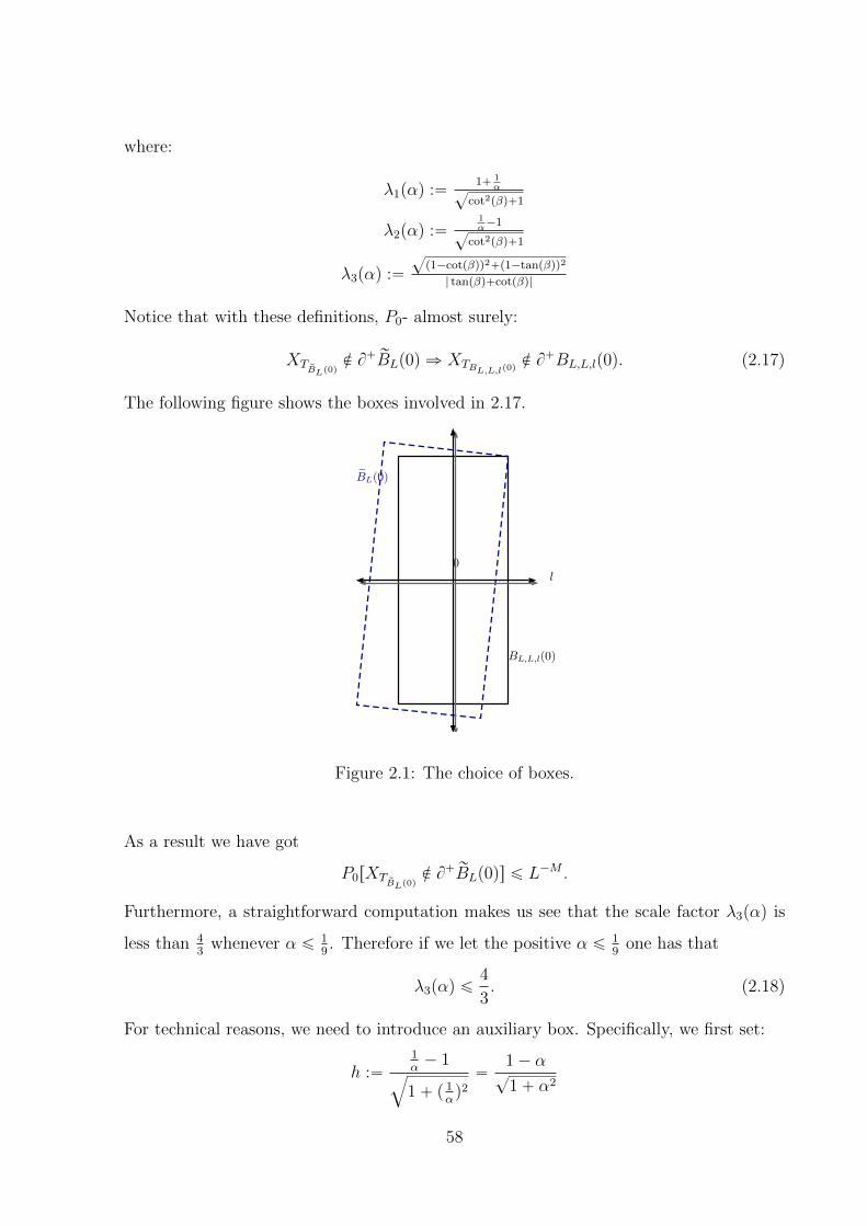
where:

λ1pαq :“1` 1

α?cot2pβq`1

λ2pαq :“1α´1

?cot2pβq`1

λ3pαq :“

?p1´cotpβqq2`p1´tanpβqq2

| tanpβq`cotpβq|

Notice that with these definitions, P0- almost surely:

XTrBLp0q

R B`rBLp0q ñ XTBL,L,lp0q

R B`BL,L,lp0q. (2.17)

The following figure shows the boxes involved in 2.17.

BL(0)

0

BL,L,l(0)

l

Figure 2.1: The choice of boxes.

As a result we have got

P0rXTrBLp0q

R B`rBLp0qs ď L´M .

Furthermore, a straightforward computation makes us see that the scale factor λ3pαq is

less than 43

whenever α ď 19. Therefore if we let the positive α ď 1

9one has that

λ3pαq ď4

3. (2.18)

For technical reasons, we need to introduce an auxiliary box. Specifically, we first set:

h :“1α´ 1

b

1` p 1αq2“

1´ α?

1` α2

58

and observe that 45ă h ă 1. We then can introduce the new box Bl´2,Lp0q defined by:

Bl´2,Lp0q :“ R1´

r´Lph` 2q, Lhs ˆ r´cLλ3pαq, Lcλ3pαqsd´1

¯

X Zd.

From this definition, we obtain:

P0rXTBl´2,Lp0qR B

`Bl´2,Lp0qs ď L´M .

In order to complete the proof, we claim that for large enough U the probability:

P0rXTBl´2,Up0qR B

`Bl´2,Up0qs.

has polynomial decay on U , where the box Bl´2,Up0q is defined by

Bl´2,Up0q :“ R1pr´U,U s ˆ r´2cU, 2cU sd´1q.

The general strategy to follow will be to stack smaller boxes up inside of Bl´2,Up0q and

then using the Markov property along with good environment sets we will ensure that the

walk exits from box Bl´2,Up0q by B`Bl´2,Up0q with probability bigger than 1 ´ 1P pUq,

where P is a polynomial function. Specifically, we let

L :“U

h` 2. (2.19)

We introduce a sequence of stopping times as follows:

T1 “ TBl´2,Lp0q,

and for i ą 1

Ti “ Ti´1 ` T1 ˝ θTi´1.

For simplicity we write pT1 instead of TBl´2,Up0q. In view of (2.18) and (2.19) it is clear that

four successful exits of the walk from boxes of the Bl´2,Lp0q-type are sufficient to ensure

that the walk exits from Bl´2,Up0q by its positive boundary. Therefore one sees that

P0rXxT1P B`Bl´2,Up0qs ě P0

“

XT1 P B`Bl´2,Lp0q,

`

XT1 P B`Bl´2,LpXT1q

˘

˝ θT1 ,`

XT1 P B`Bl´2,LpXT2q

˘

˝ θT2 ,`

XT1 P B`Bl´2,LpXT3q

˘

˝ θT3‰

(2.20)

59

In order to use (2.20), let i be a positive integer number and consider the lattice sets

sequence pFiqiě1 defined by:

F1 “ B`Bl´2,Lp0q,

and for i ą 1, we define by induction:

Fi “ď

yPF1

B`Bl´2,Lpyq.

We now define for i ě 1, the environment events Gi by:

Gi “

ω P Ω : Py,ωr`

XT1 P B`Bl´2,LpXTiq

˘

˝ θTis ě 1´ L´M2 , for each y P Fi

)

Plainly it is satisfied

P0rXxT1P B`Bl´2,Up0qs ě

P0

“

XT1 P B`Bl´2,Lp0q,

`

XT1 P B`Bl´2,LpXT1q

˘

˝ θT1 ,`

XT1 P B`Bl´2,LpXT2q

˘

˝ θT2 ,`

XT1 P B`Bl´2,LpXT3q

˘

˝ θT3‰

ě

P0

“

XT1 P B`Bl´2,Lp0q,

`

XT1 P B`Bl´2,LpXT1q

˘

˝ θT1 ,`

XT1 P B`Bl´2,LpXT2q

˘

˝ θT2 ,`

XT1 P B`Bl´2,LpXT3q

˘

˝ θT31G3

‰

By the Markov property applied at time T3 and the very meaning of G3, we get that the

last expression equals:

ř

yPF3E“

P0,ω

“

XT1 P B`Bl´2,Lp0q,

`

XT1 P B`Bl´2,LpXT1q

˘

˝ θT1 ,

`

XT1 P B`Bl´2,LpXT2q

˘

˝ θT2‰

Py,ωrXTBl´2,LpyqP B`Bl´2,Lpyqs1G3

ě

p1´ L´M2 q

`

P0

“

XT1 P B`Bl´2,Lp0q,

`

XT1 P B`Bl´2,LpXT1q

˘

˝ θT1 ,`

XT1 P B`Bl´2,LpXT2q

˘

˝ θT2‰

´ PrpG3qcs˘

(2.21)

. (2.22)

Repeating the above argument, one has the following upper bound for the right most

expression of (2.21):

p1´ L´M2 q

4´ p1´ L´

M2 q

3PrpG1qcs ´ p1´ L´

M2 q

2PrpG2qcs ´ p1´ L´

M2 qPrpG3q

cs. (2.23)

60

At this point, we would like to obtain for i P |r1, 3s|, an upper bound of the probabilities:

PrpGiqcs.

To this end, we first observe that Chevyshev’s inequality and our hypothesis imply:

PrpG1qcs ď

ÿ

yPF1

Er1tPy,ωrXT

Bl´2,LpyqPB`Bl´2,L

pyqsąL´M2 us ď| F1 | L

´M2 .

Clearly, we have the estimate | F1 |ď`

83L˘d´1

(recall (2.18)). As a result, we have that:

PrpG1qcs ď

ˆ

8

3L

˙d´1

L´M2 . (2.24)

By a similar procedure we can conclude that

PrpG2qcs ď

ˆ

16

3L

˙d´1

L´M2 . (2.25)

and

PrpG3qcs ď

ˆ

24

3L

˙d´1

L´M2 . (2.26)

Combining the estimates in (2.20)-(2.26) and the assumption M ě 6pd´ 1q we see that:

P0rXxT1R B

`Bl´2,Up0qs ď 36p8qd´1

2´M3

U´M3 .

This ends the proof by choosing the required α as any number in the open interval

p0, 19q.

2.3 Examples of directionally transient random walks

without an asymptotic direction and vanishing

velocity

We will present two examples of random walks in random environment which exhibit the

possible limitations of the hypothesis of a theorem stating the existence of an asymptotic

direction and of a theorem stating the existence of a non-vanishing velocity for mixing

environments.

61

Assumption TNB.

Let p be a random variable taking values in p0, 1q such that there exists a unique

κ P p12, 1q with the property that

Erρκs “ 1 and Erρκ ln` ρs ă 8,

where ρ :“ p1´ pqp.

2.3.1 Random walk with a vanishing velocity but with an asymp-

totic direction

Let tpi : i P Zu be i.i.d. copies of p. Let e1 and e2 be the canonical vectors in Z2. Define an

i.i.d. sequence of random variables tωi : i P Zu with ωi “ tωipe1q, ωip´e1q, ωipe2q, ωip´e2qu,

by

ωipe2q “ ωip´e2q “1

4,

ωipe1q “pi2

and ωip´e1q “1

2´pi2.

Now consider the random environment ω “ tωppi, jqq : pi, jq P Z2u defined

ωppi, jqq :“ ωi for all i, j P Z.

We will call P1 the law of the above environment and Q1 the annealed law of the corre-

sponding random walk starting from 0.

Theorem 2.3.1. Consider a random walk in a random environment with law P1. Then,

the following are satisfied:

piq Q1-a.s.

limnÑ8

Xn ¨ e1 “ 8.

62

piiq Q1-a.s.

limnÑ8

Xn

n“ 0.

piiiq In Q1-probability

limnÑ8

Xn

|Xn|2“ e1.

pivq The law Q1 satisfies the polynomial condition pPCqM,c is satisfied, with M “ κ´ 12´ε

and c “ 1, where ε is an arbitrary number in the interval p0, κ´ 12q.

Proof.

piq We will describe a one dimensional procedure which will be used throughout the

proofs of items (i) and piiq. Specifically, defining pYnqně0 :“ pXn ¨ eiqně0 one has

that it can be identified with the one dimensional RWRE which has quenched law

P0,ω starting from 0, defined by the transition probabilities:

P0,ωrYn`1 “ Yn ` e1 | Yns “ rωpYn, e1q “ pYn2,

P0,ωrYn`1 “ Yn ´ e1 | Yns “ rωpYn,´e1q “ p1´ pYnq2, and

P0,ωrYn`1 “ Yn | Yns “ rωpYn, 0q “ 12.

Since assumption TNB it follows that rE1rlnr rρ0ss ă 0, where rρ0 :“ rωp0,´e1qrωp0, e1q

and rE1 denotes the corresponding expectation in this random environment. Now,

from the transience criteria in [Ze1] Theorem 2.1.2 one has that Q1- a.s.

limnÑ8

Xn ¨ e1 “ 8.

piiq Since κ ď 1, using a one dimensional procedure for directions e1 and e2 and the

strong law of large numbers for one dimensional RWRE ([Ze1], Theorem 2.1.9), we

get Q1-a.s.Xn

n“pXn ¨ e1qe1 ` pXn ¨ e2qe2

nÑ 0.

63

piiiq We define the random variables N1 and N2 as horizontal and vertical steps performed

by the walk Xn, respectively. By the very definition of this example, both of them

distribute Bpn, 12q under the quenched law. Given ε ą 0, we have to estimate the

following probability:

Q1

«ˇ

ˇ

ˇ

ˇ

ˇ

pXn ¨ e1qe1 ` pXn ¨ e2qe2a

pXn ¨ e1q2 ` pXn ¨ e2q

2´ e1

ˇ

ˇ

ˇ

ˇ

ˇ

ą ε

ff

“ Q1

»

–

ˇ

ˇ

ˇ

ˇ

ˇ

ˇ

pXn¨e1qnκ

e1 `pXn¨e2qnκ

e2b

pXn¨e1q2

n2κ `pXn¨e2q2

n2κ

´ e1

ˇ

ˇ

ˇ

ˇ

ˇ

ˇ

ą ε

fi

fl .

Clearly, Xn ¨ e2 under the annealed law has the same law rP of the one dimensional

simple symmetric random walk Zn1 at time n1 “ N2, such that rP - a.s. n1n Ñ 12

as nÑ 8. Therefore, since κ ą 12 as a result one has

Q1

„

limnÑ8

Xn ¨ e2

nκ“ 0

“ rP

„

limN2Ñ8

ZN2

Nκ2

1

2κ“ 0

“ 1.

and also Q1- a.s.

limnÑ8

pXn ¨ e2q2

n2κ“ 0.

On the other hand, using the convergence theorem of Kesten, Kozlov and Spitzer

[KKS75], calling YN1 the one dimensional random walk in random environment

corresponding to Xn ¨ e1 and using a similar procedure as the one given above, we

can see thatXn ¨ e1

a

pXn ¨ e1q2Ñ 1

in distribution, which turns out that this convergence is also in Q1- probability and

completes the proof.

pivq For j P t1, 2u and a a positive real number, we define the stopping times Teja and

rTeja by

T eja :“ inftn ě 0 : Xn ¨ ej ě au (2.27)

along with

rT eja :“ inftn ě 0 : Xn ¨ ej ď au (2.28)

Notice that for c “ 1 and large L one has the following estimate

Q1rXTBL,cL,l p0qR B

`BL,cL,lp0qs ď Q1rrTe1´L ă T e1L s `Q1rT

e2L ^ rT e2´L ă T e1L s. (2.29)

64

The first probability in the right most side of (2.29) has an exponential bound as it

follows from the estimate in the proof of item pivq in Theorem 2.3.2. Observe that

the second probability in the right most side of (2.29) is less than or equal to

Q1rTe2L ^ rT e2´L ď L2`ε

s `Q1rL2`ε

ă T e1L s.

Keeping the notations introduced in item piiiq. From the very definition of Z 1n, one

sees that for large L, there exists a positive constant K1 such that:

Q1rTe2L ^ rT e2´L ď L2`εs ď Q1r|Xn ¨ e2| ď L, for all n P N, 0 ď n ď L2`εs ď

rP rZN2pnq ď L2`ε, for all n P N, 0 ď n ď L2`εs ď expt´K1Lεu. (2.30)

On the other hand, using the sharp estimate in Theorem 1.3 in [FGP10] and denoting

P the law of underlying one dimensional random walk corresponding to the annealed

law of pXn ¨ e1qně0, we can see that for large L, there exists a positive constant K2

such that:

Q1rL2`ε ă T e1L s ď Q1rXrL2`εs ¨ e1 ă Ls ď

P rYN1prL2`εsq ă Ls ď K2L´pκ´12´εq. (2.31)

(2.32)

Therefore, in view of the inequality (2.29) and the estimates (2.30)-(2.31), we com-

plete the proof.

2.3.2 Directionally transient random walk without an asymp-

totic direction

Let tpi : i P Zu and tp1j : j P Zu be two independent i.i.d. copies of p. Following a similar

procedure as in the previous example, we consider in the lattice Z2 the canonical vectors

e1 and e2, and define the random environment ω “ tωppi, jqq : pi, jq P Z2u by,

65

ωpi,jqpe1q “pi2

and ωpi,jqp´e1q “1

2´pi2.

together with

ωpi,jqpe2q “p1j2

and ωpi,jqp´e2q “1

2´p1j2.

We call P2 the law of the above environment and Q2 the annealed law of the corresponding

random walk starting from 0.

Theorem 2.3.2. Consider a random walk in a random environment with law P2. Then,

the following are satisfied.

piq Let l P S. Then l ¨ e1 ě 0 and l ¨ e2 ě 0 if and only if Q2-a.s.

limnÑ8

Xn ¨ l “ 8.

piiq Q2-a.s.

limnÑ8

Xn

n“ 0.

piiiq There exists a non-deterministic v such that:

Xn

|Xn|2Ñ v.

in distribution.

pivq There exists a c ą 1 such that

limLÑ8L´1 logQ2rXTBL,cL,l p0q

R B`BL,cL,lp0qs ă 0, (2.33)

where l “ p1?

2, 1?

2q. Thus, condition pT q|l [Sz02] is satisfied.

Proof.

66

piq This amounts to prove that Q2- a.s.

limnÑ8

Xn ¨ e1 “ 8 and limnÑ8

Xn ¨ e2 “ 8.

Both assertions follow from the one dimensional procedure, Theorem 2.1.2 in [Ze1]

and the assumption TNB.

piiq This proof is similar to case piiq of Theorem 2.3.1 .

piiiq Define a sequence Ti,j, for i ě 0, j P t1, 2u as follows: T0,j “ 0,

T1,j “ inftn ě 0 : pXn ´X0q ¨ ej ą 0 or pXn ´X0q ¨ ej ă 0u

and for i ě 2

Ti,j “ T1,j ˝ θTi´1,j` Ti´1,j.

Setting Yn,j :“ XTn,j ¨ ej, we see that for j P t1, 2u, the one dimensional random

walks without transitions to itself at each site pYn,jqně0 are independent and their

transitions at each site i P Zd are determined by pi. Furthermore, for j P t1, 2u, the

strong law of large numbers implies that Q2- a.s.

limnÑ8

Tn,jn“ 2. (2.34)

We now apply the result of Kesten, Kozlov and Spitzer [KKS75] to see that there

exist constants C1 and C2 such that

ˆ

Yn,1nκ

,Yn,2nκ

˙

Ñ

ˆ

C1

ˆ

1

S1 κca

˙κ

, C2

ˆ

1

S2 κca

˙κ˙

in distribution, where for j P t1, 2u, Sj κca stand for two independent completely

asymmetric stable laws of index κ, which are positive. Using (2.34) and properties

of convergence in distribution we can see that

Xn

|Xn|“

pXn¨e1qnκ

e1 `pXn¨e2qnκ

e2b

pXn¨e1q2

n2κ `pXn¨e2q2

n2κ

Ñ

´

C1

S1 κca

¯κ

e1 `

´

C2

S2 κca

¯κ

e2

c

´

C1

S1 κca

¯2κ

`

´

C2

S2 κca

¯2κ

in distribution. Therefore we have proved that the limit v is random.

67

pivq A first step will be to prove the following decay

lim supL´1 logQ2rrTej´rcL ă T

ejcLs ă 0

for arbitrary positive constants rc and c (see (2.27) and (2.28) for the notations). We

prove this in the case j “ 1, the another case being similar. Following the notation

introduced in Theorem 2.3.1 item piq and denoting the greatest integer function

by r¨s, we see that it is sufficient to prove that for large L there exists a positive

constant pC such that:

rE1rP0,ωrYn hits rpcLs ` 1 before rcLs ` 1ss ď expt´ pCLu. (2.35)

To this end, for a fixed random environment ω, if we denote VLi to

Pi,ωrYn hits ´ rpcLs ` 1 before rcLs ` 1s,

the Markov property makes us see that VLi satisfies the following difference equation

for integer i P rrcLs ` 2, rcLss

VLi “ p1´ piqV

Li´1 ` p1V

Li`1

with the constraints

VLrrcLs`1 “ 1 and VL

rcLs`1 “ 0.

This system can be solved by the method developed by Chung in [Ch67], Chapter

1, Section 12. Applying this one sees that

VL0 “

exptř

´rpcL`1s,0u ` . . .` exptř

´rpcLs`1,rcLsu

1` exptř

´rpcLs`1,´rpcLs`2u ` . . .` exptř

´rpcLs`1,rcLsu,

where we have adopted the notation introduced in [Sz02],ř

zămďz1 “ log ρpmq and

ρpmq “ p1´pmqpm. A slight variation of the argument in [Sz02] page 744 completes

the proof of claim (2.35). On the other hand, considering the probability

Q2rXTBL,2L,l p0qR B

`BL,2L,lp0qs,

we observe that is clearly bounded from above by (see Figure 2.2)

Q2rrTe1

´?22Lă T e1?

2Ls `Q2rrT

e2

´?22Lă T e2?

2Ls

In virtue of the claim (2.35) the last expression has an exponential bound and this

finishes the proof.

68

(1√2, 1√

2

)

L

2L

Slab H1

SlabH

2

Figure 2.2: A geometric sketch to bound Q2rXTBL,2L,l p0qR B`BL,2L,lp0qs.

2.4 Backtracking of the random walk out of a cone

Here we will provide a uniform control on the probability that a random walk starting

form the vertex of a cone stays inside the cone forever. It will be useful to this end to

define

D1 :“ inftn P N : Xn R Cpα, l,X0qu, (2.36)

where as before l P Sd´1.

Proposition 2.4.1. Let l P Sd´1. Suppose that pP qM,c|l holds, for some M ą 6d ´ 3.

Then there exists a positive constant c2pdq ą 0 such that P0rD1 “ 8s ą c2pdq.

In what follows we prove this proposition. With the purpose of making easier the

reading, we introduce here some notations. Let l1 P Sd´1 and choose a rotation R1 on Rd

with the property

R1pe1q “ l1

For each x P Zd, real numbers m ą 0, c ą 0 and integer i ě 0 we define the box

Bipxq :“

x`R1´

p´2m`i, 2m`iq ˆ p´2c2m`i, 2c2m`iqd´1

¯

X Zd

69

along with its ”positive boundary”

B`Bipxq :“ BBipxq X tx`R

1`

p2m`i,8q ˆ Rd´1˘

u.

We also need slabs perpendicular to direction l1. Set

V0pxq :“ x`R1`

r´2m, 2ms ˆ Rd´1˘

X Zd

and for i ě 1,

Vipxq :“ x`R1

˜«

´2m,iÿ

j“0

2m`j

ff

ˆ Rd´1

¸

X Zd.

The positive part of the boundary for this set is defined as

B`Vipxq :“ BVipxq X

#

x`R1

˜˜

iÿ

j“0

2m`j,8

¸

ˆ Rd´1

¸+

.

Furthermore, we will define recursively a sequence of stopping times as follows. First, let

T0 :“ TB0pX0q.

and for i ě 1

Ti :“ TBipXTi´1q ˝ θTi´1

` Ti´1.

We now need to define the first time of entrance of the random walk to the hyperplane

R1`

p´8, 0q ˆ Rd´1˘

,

Dl1 :“ inftn ě 0 : Xn ¨ l1ă 0u.

With these notations we can prove:

Lemma 2.4.2. Assume pP qN,2c|l1 where c ą 0 , for some N ą 2pd ´ 1q. Then, for all

m P N and x P tz P Zd : z ¨ l1 ě 2mu, we have that

PxrDl1 “ 8s ě ypmq

where ypmq does not depend on l1 and satisfies limmÑ8 ypmq “ 1.

70

Proof. From the fact that pP qN,2|l1 holds, we can (and we do) assume that there exists a

m ą 0 large enough, such that for any positive integer i one has that

P0rXTBip0qP B

`Bip0qs ě 1´ 2´Npm`iq (2.37)

holds. By stationarity, we have for x P Zd:

PxrXTBipxqP B

`Bipxqs ě 1´ 2´Npm`iq. (2.38)

Throughout this proof, let us choose x P tz P Zd : z ¨ l1 ě 2mu. For reasons that will be

clear through the proof, we need to estimate for i ě 1 the following probability

Ii :“ PxrXTVipxqP B

`Vipxqs, (2.39)

and with this aim, in view of (2.38), we have

I0 ě PxrXTB0pxqP B

`B0pxqs ě 1´ 2´Nm ě 1´ 2´Nm2 .

Now, as a preliminary computation for the recursion, we begin to estimate I1. Note that

I1 ě PxrXT0 P B`B0pX0q, pXTB1pX0q

P B`B1pX0qq ˝ θT0s. (2.40)

Using the strong Markov property at time T0 we then see that

I1 ěř

yPB`B0pxqE rPx,ωrXT0 P B

`B0pX0q, XT0 “ ys

ˆ Py,ωrXTB1pyqP B`B1pyqs

ı

ěř

yPB`B0pxqE rPx,ωrXT0 P B

`B0pX0q, XT0 “ ys

ˆ Py,ωrXTB1pyqP B`B1pyqs1G0

ı

, (2.41)

where

G0 :“

tw P Ω : Py,ωrXTB1pyqP B`B1pyqs ą 1´ 2´N

m2 , for all y P B`B0pxqu.

71

Thus, it is clear that

I1 ě`

1´ 2´Nm2

˘ `

PxrXT0 P B`B0pX0qs ´ PrpG0q

cs˘

. (2.42)

Notice that by (2.38) and Chebyshev’s inequality

PrpG0qcs ď

ř

yPB`B0pxqPrPy,ωrXTB1pyq

R B`B1pyqs ě 2´Nm2 s

ďř

yPB`B0pxqPyrXTB1pyq

R B`B1pyqs2N m

2

“ |B`B0pxq|2N m

2 sP0rXTB1p0qR B`B1p0qs

ď p2c2m`1qd´12Npm2´pm`1qq ď p2c2m`1qd´12´N

m2 . (2.43)

Plugging (2.43) into (2.42) we see that

I1 ě p1´ 2´Nm2 qp1´ 2´N

m2 ´ p2c2m`1

qd´12´N

m2 q. (2.44)

Hereafter we can do the general recursive procedure. For this end, we define for i ě 1

Ji :“ P0rXT0 P B`B0pX0q, pXTB1pX0q

P B`B1pX0qq ˝ θT0 , . . .

. . . , pXTBipX0qP B

`BipX0qq ˝ θTi´1s.

(2.45)

It is straightforward that Ii ě Ji. Furthermore, through induction on i ě 1, we will

establish the following claim

Ji ě p1´ 2´Npm`i´1q

2 q

»

–Ji´1 ´ 2´Npm`i´1q

2

˜

i´1ÿ

j“0

2c2pm`jq`1

¸d´1fi

fl . (2.46)

To prove this, we first define the extended boundary of the pile of boxes at a given step as

F0 :“ BB0pxq X tx`R1pp2m,8q ˆ Rd´1

qqu,

and for i ě 2

Fi´1 :“ B

YyPFi´2Bi´1pyq

(

X tx`R1pp2m`i´1,8q ˆ Rd´1qqu.

Using these notations, we can apply the strong Markov property to (2.45) at time Ti´1,

to get that

Ji “ř

yPFi´1E rPx,ωrXT0 P B

`B0pX0q, . . .

. . . , pXTBi´1pX0qP B`Bi´1pX0qq ˝ θTi´2

, XTi´1“ ysPy,ωrXTBipX0q

P B`BipX0qs

ı

.

72

Following the same strategy used to deduce (2.44), it will be convenient to introduce for

each i ě 2 the event

Gi´1 :“

tω P Ω : Py,ωrXTBipyqP B`Bipyqs ą 1´ 2´N

pm`i´1q2 , for all y P Fi´1u.

Inserting the indicator function of the event Gi´1 into (2.45) we get that

Ji ě

ř

yPFi´1E”

Px,ωrXT0 P B`B0pX0q, . . . , pXTBi´1pX0q

P B`Bi´1pX0qq ˝ θTi´2, XTi´1

“ ys

ˆPy,ωrXTBipX0qP B`BipX0qs1Gi´1

ı

.

By the same kind of estimation as in (2.42), we have

Ji ě p1´ 2´Npm`i´1q

2 q pJi´1 ´ PrpGi´1qcsq . (2.47)

We need to get an estimate for PrpGi´1qcs. We do it repeating the argument given in

(2.43). Let us first remark that

|Fi´1| ď

˜

i´1ÿ

j“0

2c2pm`jq`1

¸d´1

, (2.48)

holds. Indeed, the case in which l1 “ e1 gives the maximum number for |Fi´1|. Keeping

(2.48) in mind we get that

PxrpGi´1qcs ď

ř

yPFi´1P”

Py,ω

”

XTBipyqR B`Bipyq

ı

ě 2´Npm`i´1q

2

ı

ďř

yPFi´1PyrXTBipyq

R B`Bipyqs2N pm`i´1q

2

ď

´

ři´1j“0 2c2pm`jq`1

¯d´1

2´Npm`i´1q

2 . (2.49)

Therefore, combining (2.49) and (2.47) we prove claim (2.46). Iterating (2.46) backward,

from a given integer i, we have got

Ji ě J1

«

i´1ź

h“1

p1´ 2´Npm`hq

2 q

ff

´

i´1ÿ

j“1

aj2´N m`j

2

i´1ź

k“j

p1´ 2´Npm`kq

2 q, (2.50)

where we have used for short

aj :“

˜

jÿ

i“0

c2pm`iq`1

¸d´1

ď p2cqd´12pm`j`2qpd´1q.

73

The same argument used to derive (2.44) can be repeated to conclude that

J1 ě p1´ 2´Nm2 qp1´ 2´N

m2 ´ p2c2m`1

qd´12´N

m2 q. (2.51)

Replacing the right hand side of (2.51) into (2.50), and together to the fact Ii ě Ji, we

see that

Ii ě

«

i´1ź

h“0

p1´ 2´Nm`h

2 q

ff

p1´ 2´Nm2 q ´

i´1ÿ

j“0

aj2´N pm`jq

2

i´1ź

k“j

p1´ 2´Npm`kq

2 q. (2.52)

Now we can finish the proof. First, observe that

PxrDl1 “ 8s ě I8,

where as a matter of definition

I8 :“ limiÑ8

Ii

(this limit exists, because it is the limit of a decreasing sequence of real numbers bounded

from below). By the condition N ą 2pd´ 1q, we get that for each m ě 1 one has that for

all j ě 1,

aj 2´Mpm`jq

2 ď p8cqd´12´ϑpm`jq

2 ,

where ϑ stands for the positive number so that N “ 2pd´ 1q ` ϑ. Thus all the products

and series in (2.52) converge and we have that for all m ě 1 and x P tz P Zd : z ¨ l1 ě 2mu

PxrDl1 “ 8s ě ypmq,

where

ypmq :“”

ś8

h“0p1´ 2´Npm`hq

2 q

ı

p1´ 2´Nm2 q

´ř8

j“0 aj2´N pm`jq

2

ś8

k“jp1´ 2´Npm`kq

2 q.

Clearly for each m ě 1, ypmq does not depend on the direction l1 and limmÑ8 ypmq “ 1,

which completes the proof.

74

With the previous Lemma, we now have enough tools to prove Proposition 2.4.1.

Before this, we need a definition of geometrical nature.

We will say that a sequence px0, . . . , xnq of lattice points is a path if for every 1 ď i ď

n´ 1, one has that xi and xi´1 are nearest neighbors. Furthermore, we say that this path

is admissible if for every 1 ď i ď n´ 1 one has that

pxi ´ xi´1q ¨ l ‰ 0.

Proof of Proposition 2.4.1. Assume pP qM,c|l, where M ą 6pd ´ 1q ` 3 which is the con-

dition of the statement of the Proposition 2.4.1. We appeal to Proposition (2.2.3) and

assumption pP qM,c|l to choose an α ą 0 such that for all i P r2, ds

pP qN,2c|l˘i

is satisfied with

N :“M

3´ 1 ą 2pd´ 1q. (2.53)

From now on, let m be any natural number satisfying

ypmq ą 1´1

2pd´ 1q, (2.54)

where ypmq is the function given in Lemma 2.4.2. Note that there exists a constant c3pdq

such that for all x P Zd contained in Cpα, l, Rp2me1qq and such that |Rp2me1q ´ x|1 ď 1

one has that there exists an admissible path with at most c32m lattice points joining 0

and x. We denote this path by

p0, y1, . . . , yn “ xq

noting that n ď c32m.

The general idea to finish the proof is to push forward the walk up to site x with the

help of uniform ellipticity in direction l and then we make use of Lemma (2.4.2) to ensure

that the walk remains inside the cone.

75

Therefore, by (2.53) and Lemma (2.4.2) we can conclude that for all 2 ď i ď d one

has that

PxrDli` “ 8s ě ypmq, (2.55)

along with

PxrDli´ “ 8s ě ypmq. (2.56)

Define the event that the random walk starting from 0 following that path p0, y1, . . . , ynq

as

An :“ tpX0, . . . , Xnq “ p0, y1, . . . , ynqu.

Now notice that

P0rD1“ 8s ě

P0

“

An, pDli´ “ 8q ˝ θn, p Dli` “ 8q ˝ θn for 2 ď i ď d‰

. (2.57)

On the other hand, by definition of the annealed law, together with the strong Markov

property we have that

P0rAn, pDli´ “ 8q ˝ θn, p Dli` “ 8q ˝ θn for 2 ď i ď ds “

E“

P0,ωrAns, Px,ωrDli´ “ 8, Dli` “ 8 for 2 ď i ď ds‰

. (2.58)

Using the uniform ellipticity assumption pUEq|l, along with (2.55) and (2.56), we can see

that (2.58) is bounded from below by

p2κqc32mp1´ 2pd´ 1qp1´ ypmqqq . (2.59)

By virtue of our choice of m in (2.54), we see that there exists a constant c2 just depending

on the dimension (we recall that m is fixed at this point of the proof), such that

c4 :“ p2κqc32mp1´ 2pd´ 1qp1´ ypmqqq ą 0 (2.60)

Finally, in view of the inequalities (2.57) and (2.58) it follows that

P0rD1“ 8s ě c4.

76

2.5 Polynomial control of regeneration positions

In this section, we define an approximate regeneration times as done in [CZ01], which will

depend on a distance parameter L ą 0. We will then show that these times, assuming

pPCqM,c|l for M large enough, and cone-mixing, when scaled by κL, define approximate

regeneration positions with a finite second moment.

2.5.1 Preliminaries

We recall the definition of approximate renewal time given in [CZ01]. Let W :“ E Y t0u

[c.f. (2.2)] and endow the space WN with the canonical σ´algebra W generated by the

cylinder sets. For fixed ω P Ω and ε “ pε0, ε1, . . .q P WN, we denote by Pω,ε the law of the

Markov chain tXnu on pZdqN, so that X0 “ 0 and with transition probabilities defined for

z P Zd, e, |e| “ 1 as

Pω,εrXn`1 “ z ` e|Xn “ zs “ 1tεn“eu `1tεn“0u

1´ κ|E |rωpz, eq ´ κ1tePEus.

Call Eω,ε the corresponding expectation. Define also the product measure Q, which to

each sequence of the form ε P WN assigns the probability Qpε1 “ eq :“ κ, if e P E , while

Qpε1 “ 0q “ 1´ κ|E |, and denote by EQ the corresponding expectation.

Now let G be the σ-algebra on pZdqN generated by cylinder sets, while F be the σ-

algebra on Ω generated by cylinder sets. Then, we can define for fixed ω the measure

P 0,ω :“ Qb Pω,ε

on the space pWN ˆ pZdqN,W ˆGq, and also

P 0 :“ PbQb Pω,ε

on pΩˆWNˆpZdqN,FˆWˆGq, denoting by E0,ω and E0 the corresponding expectations. A

straightforward computation makes us conclude that the law of tXnu under P0,ω coincides

with its law under P0,ω and that its law under P 0 coincides with its law under P0.

Let q be a positive real number such that for all 1 ď i ď d,

77

ui :“ liq

is an integer. Define now the vector u :“ pu1, . . . , udq. From now on, we fix a particular

sequence ε in E of length p :“ |u|1 whose components sum up to u:

ε :“ pε1, . . . , εpq,

together with

ε1 “ ε2 “ . . . “ ε|u1| :“ sgnpu1qe1,

ε|u1|`1 “ ε|u1|`2 “ . . . “ ε|u1|`|u2| :“ sgnpu2qe2

...

εp´|ud|`1 “ . . . “ εp :“ sgnpudqed.

Without loss of generality we can assume that l1 ­“ 0. And by taking α small enough that

ε1, ε1 ` ε2, . . . εp

are inside of Cp0, l, αq. For L P pN consider the sequence εpLq of length L, defined as the

concatenation Lp times with itself of the sequence ε, so that

εpLq “ pε1, . . . , εp, . . . , ε1, . . . , εpq.

Consider the filtration G :“ tGn : n ě 0u where

Gn :“ σppεi, Xiq, i ď nq.

Define S0 :“ 0,

S1 :“

inftn ě L : Xn´L ¨ l ą maxtXm ¨ l : m ă n´ Lu, pεn´L, . . . , εn´1q “ εpLqu

together with

R1 :“ D1 ˝ θS1 ` S1.

78

We can now recursively define for k ě 1,

Sk`1 :“

inftn ě Rk : Xn´L ¨ l ą maxtXm ¨ l : m ă n´ Lu, pεn´L, . . . , εn´1 “ εpLqqqu

and

Rk`1 :“ D1 ˝ θSk`1` Sk`1.

Clearly,

0 “ S0 ď S1 ď R1 ď ¨ ¨ ¨8,

the inequalities are strict if the left member of the corresponding inequality is finite, and

the sequences tSk : k ě 0u and tRk : k ě 0u are G-stopping times. On the other hand, we

can check that P0´a.s. one has that S1 ă 8 along with the fact P0´a.s. on the set

tlimXn ¨ l “ 8u X tRk ă 8u one has too that (2.61)

Sk`1 ă 8.

Put

K :“ inftk ě 1 : Sk ă 8, Rk “ 8u

and define the approximate regeneration time

τ pLq :“ SK . (2.62)

We see that the random variable τ pLq is the first time n in which the walk has reached a

record at time n ´ L in direction l, and then the walk goes on L steps in the direction l

by means of the action of εpLq to finally after this time n never exits the cone CpXn, l, αq.

The following lemma is required to show that the approximate renewal times are P0-

a.s. finite. Its can be proved using a slight variation of the argument given in page 517

of Sznitman [Sz03].

Lemma 2.5.1. Consider a random walk in a random environment. Let l P S˚d´1, M ě

d`1 and c ą 0 and assume that pPCqM,c|l is satisfied. Then the random walk is transient

in direction l.

79

Proof. For the sake of completeness, we are going to sketch the steps so as to obtain the

claim of the theorem.

Step 1. Notice that any M ą 0 gives

P0rlim supnÑ8

Xn ¨ l “ 8s “ 1.

From one can easily show that

P0rlim supnÑ8

Xn ¨ l “ 8s “ 1

if and only if

limLÑ8

P0rinftn ě 0 : Xn ¨ l ě Lu “ 8s “ 0.

Step 2. Following the argument on page 517 of [Sz03], we have got to get rid the order

of the positive boundary of a box plus some order which makes possible to apply Borel-

Cantelli Lemma. It can be seen that a term in M of d´ 1 suffices to get rid the order of

the positive boundary and therefore M ě pd´ 1q ` 2 “ d` 1 is enough to get:

P0r limnÑ8

Xn ¨ l “ 8s “ 1.

We make note a trivial remark that the random walk is transient in direction u also.

We can now prove the following stronger version of Lemma 2.2 of [CZ01].

Lemma 2.5.2. Assume pCMqα,φ|l, pUEq|l and pPCqM,c for M ą 6d ´ 3, c ą 0. Then

there exists a positive L0 P |u|1N, such that

φpL0q ` P0rD1ă 8s ă 1,

and τ pLq ă 8, P0-a.s. are fulfilled for each L ě L0, L P |u|1N.

Proof. Following the arguments in the proof of Lemma 2.2. of [CZ01] (using u instead of

l), one has that:

P0rRk ă 8s ď pφpL0q ` P0rD1ă 8sq

k (2.63)

80

From the assumption pCMqα,φ|l, we have φpLq Ñ 0 as L Ñ 8. On the other hand, by

Lemma 2.4.1,

P0rD1ă 8s ă 1.

Therefore, we can find a L0 with the property:

φpLq ` P0rD1ă 8s ă 1,

for all L ě L0, L P N|l|1.

Then, via Borel-Cantelli Lemma, one has that P0´ almost surely

inftn ě 1 : Rn “ 8u ă 8, (2.64)

holds. Now, observe that P0´ almost surely:

inftn ě 1 : Rn “ 8u “ inftn ě 1 : Rn´1 ă 8 Rn “ 8u (2.65)

In turn, using (2.61) which is satisfied in view of Lemma 2.5.1, turns out that

inftn ě 1 : Sn ă 8 Rn “ 8u “ K ă 8

P0´ almost surely.

Finally, we can state the following proposition, which gives a control on the second moment

of the position of the random walk at the first regeneration position. Define for x P Zd

and L ą 0 the σ´algebra

Fx,L :“ σ

"

ωpy, ¨q; y ¨ u ď x ¨ u´L

|u|1|u|2

*

.

Proposition 2.5.3. Fix l P S˚d´1, α ą 0, M ą 0 and φ : r0,8q Ñ r0,8q such that

limrÑ8 φprq “ 0. Assume that 0 ă α ă mint19, 1

2c`1u and that pCMqα,φ|l, pUEq|l and

pPCqM,c|l hold. Then, there exists a constant c5, such that

E0rpκLXτ pLq ¨ lq

2|F0,Ls ď c5. (2.66)

81

2.5.2 Preparatory results

Now we are in position to prove the main proposition of this section. Before we do this,

we will prove a couple of lemmas.

Lemma 2.5.4. Assume that pCMqα,φ|l holds. Then, for each x P Zd one has that

|ErPx,ωrD1 “ 8s|Fx,Ls ´ P0rD1“ 8s| ď φpLq

holds a.s.

Proof. For each A P Fx,L, we define

νrAs :“ ErPx,ωrD1 “ 8s1As (2.67)

and

µrAs :“ pP0rD1“ 8s ` φpLqqPrAs ´ νrAs. (2.68)

Clearly (2.67) defines a measure on pΩ,Fx,Lq. We will show that (2.68) also. Indeed,

take an A P Fx,L and note that Px,ωrD “ 8s is σtωpy, ¨q, y P Cpx, l, αqu-measurable.

Therefore, by assumption pCMqα,φ|l one has that

νrAs ď P0rD1“ 8sPrAs ` φpLqPrAs.

Consequently, (2.68) defines a measure µ on pΩ,Fx,Lq. Consider the increasing sequence

tAn : n ě 1u of Fx,L-measurable sets defined by

An :“

"

ω P Ω : ErPx,ωrD1 “ 8s|Fx,Ls ą P0rD1“ 8s ` φpLq `

1

n

*

and define

A :“ď

ně1

An.

Observe that for each n ě 1 we have that

0 ď µpAnq “ pP0rD “ 8s ` φpLqqPrAns ´ ErErPx,ωrD1 “ 8s|Fx,Ls1Ans

ď ´ 1nPrAns.

82

Therefore, one has that for each n ě 1, PrAns “ 0 and consequently PrAs “ 0. Observing

that

A “ tω P Ω : ErPx,ωrD1 “ 8s|Fx,Ls ą P0rD1“ 8s ` φpLqu,

we see that

ErPx,ωrD1 “ 8s|Fx,Ls ´ P0rD1“ 8s ď φpLq. (2.69)

One can prove that

´φpLq ď ErPx,ωrD1 “ 8s|Fx,Ls ´ P0rD1“ 8s

following the same argument used to show (2.69), but changing the event tD1 “ 8u by

tD1 ă 8u.

The second lemma that will be needed to prove Proposition 2.5.3 is the following one. To

state it define

M :“ sup0ďnďD1

pXn ´X0q ¨ u,

D1p0q :“ inftn ě 0 : Xn R Cp0, l, αqu,

and for a P R

T la :“ inftn ě 0 : Xn ¨ l ě au and

T la :“ inftn ě 0 : Xn ¨ l ą au. (2.70)

Lemma 2.5.5. Let M ą 4d` 1 and

2c` 1 ď1

α. (2.71)

Assume that pPCqM,c|l is satisfied. Then, there exists c6 “ c6pdq ą 0 such that a.s. one

has that

E0rM2, D1 ă 8|F0,Ls ď c6.

83

P´ almost surely.

Proof. To simplify the proof, we will show that the second moment of

M1 :“ sup0ďnďD1

pXn ´X0q ¨ l

is bounded from above. Note that

E0rM12, D1 ă 8|F0,Ls ď P0rD

1 ă 8 | F0,Ls

`ř

mě0 22pm`1qP0r2m ďM1 ă 2m`1, D1 ă 8 | F0,Ls. (2.72)

Therefore, it is enough to obtain an appropriate upper bound of the probability when m

is large

P0r2mďM1

ă 2m`1, D1 ă 8 | F0,Ls.

Note that,

P0r2m ďM1 ă 2m`1, D1 ă 8 | F0,Ls

ď P0rTl2m ă D1 ă 8, T l2m`1 ˝ θT2m ą D1p0q ˝ θT2m | F0,Ls

ď P0rXT l2mR B`B2m,c2m,lp0q, T

l2m ă D1 ă 8 | F0,Ls

`P0rXT l2mP B`B2m,c2m,lp0q, T

l2m`1 ˝ θT2m ą D1p0q ˝ θT2m | F0,Ls. (2.73)

Using pPCqM,c|l, we get the following upper bound for the first term of the rightmost

expression in (2.73),

P0rXTB2m,c2m,lp0qR B`B2m,2m,lp0q, pXnq0ďnďTBip0q

Ă pH0,lqc|H0,ls

ď 2´Mm. (2.74)

As for the second term in the rightmost expression in (2.73), it will be useful to introduce

the set

Fm :“ B`B2m,c2m,lp0q.

Now, by the strong Markov property we have the bound

84

P0rXTB2m,c2m,lp0q P B

`B2m,2m,lp0q, Tl2m`1 ˝ θT l2m ą D1p0q ˝ θT l2m | F0,Ls

ďř

yPFmPyrT

l2m`1 ą D1p0q | F0,Ls. (2.75)

In order to estimate this last conditional probability, we obtain a lower bound for its

complement as follows. To simplify the computations which follow, for each x P Zd we

introduce the notation

Bx :“ B2m´1,c2m´1,lpxq.

Now, note that under the assumption (2.71) we have that

c`

2m ` 2m´1˘

ď cotpβq2m´1,

which implies that the boxes By and Bz, for all y P Fm and z P B`By, are inside the cone

Cp0, l, αq (see Figure 2.3).

By

Bz

B2m,c2m,l(0)

C(0, l, α)

l

Figure 2.3: The boxes By and Bz are inside of Cp0, l, αq.

Therefore, fixing y P Fm, it follows that

PyrTl2m`1 ă D1p0q | F0,Ls ě

ř

zPB`ByErPy,ωrXTBy

P B`By,

XTBy“ z, pXTBz

P B`Bzq ˝ θTBy s|F0,Ls. (2.76)

85

To estimate the right-hand side of the above inequality, it will be convenient to introduce

the set

Fm :“ BrYyPFmBys X tRpr2m´1

` 2m,8q ˆ Rd´1qu,

and the event

GFm :“ tω P Ω : Pz,ωrXTBzP B`Bzs ą

1´ 2´Mpm´1q

2 , for all z P Fmu.

Using the strong Markov property, we can now bound from below the right-hand side of

inequality (2.76) by

p1´ 2´Mpm´1q

2 q

´

PyrXTByP B

`By|F0,Ls ´ PyrpGFmqc|F0,Ls

¯

. (2.77)

In turn, by means of the polynomial condition and the fact that the boxes By and Bz are

inside the cone Cp0, l, αq we see that (2.77) is greater than or equal to

p1´ 2´Mpm´1q

2 q`

1´ 2´Mpm´1q´ PyrpGFmq

c|F0,Ls

˘

. (2.78)

Now, note that

PyrpGFmqc|F0,Ls ď

ř

xPFm2Mpm´1q

2 PxrXTBxR B`Bx|F0,Ls

ď |Fm|2´Mpm´1q

2 ď p4cqd´12mpd´1q2´Mpm´1q

2 . (2.79)

where in the first inequality we have used Chebyshev inequality, in the second one the as-

sumption that pPCqM,c|l is satisfied and in the third one the bound |F2m| ď p4cqd´12mpd´1q.

Consequently inserting the estimates (2.79) into (2.78) and combining this with in-

equality (2.76) we conclude that

PyrTl2m`1 ď D1p0q | F0,Ls ě p1´ 2´

Mpm´1q2 q ˆ

p1´ 2´Mpm´1q

2 ´ p4cqd´12mpd´1q2´Mpm´1q

2 q

ě 1´ 3p4cqd´12mpd´1q2´Mpm´1q

2 . (2.80)

86

Using the bound (2.80) in (2.75), together with the estimate |Fm| ď p2cqd´12mpd´1q, we

see that

P0rXTB2m,c2m,lp0q P B

`B2m,2m,lp0q, Tl2m`1 ˝ θT l2m ą D1p0q ˝ θT l2m | F0,Ls

ď 3p4cq2pd´1q22mpd´1q2´Mpm´1q

2 . (2.81)

Combining the estimates (2.81), (2.74), (2.73) with (2.72) we conclude that

E0rM12, D1 ă 8|F0,Ls

ď 1` 4p4cq2pd´1qř

mě0 22pm`1q22mpd´1q2´Mpm´1q

2

ď 1` 4p4cq2pd´1qř

mě0 2´m ď c6,

where in the second to last inequality we have used the fact that M ą 4d` 1 and c6 is a

constant that does not depend on L. This completes the proof of the Lemma.

2.5.3 Proof of Proposition 2.5.3

To simplify the computations, we introduce the notation

b “ bpLq :“ P0pD1 ă 8q ` φpLq,

b1 “ b1pLq :“ P0pD1 “ 8q ` φpLq

and EPbQ :“ EEQ. Furthermore, it will be necessary to define for each j ě 0 and n ě L`j

the events

Dj,n :“ tε P WN : pεm, . . . , εm`L´1q ‰ εpLq for all j ď m ď j ` n´ L` 1u.

The following lemma, whose proof is presented in Appendix 2.7, will be useful in the proof

of Proposition 2.5.3.

Lemma 2.5.6. There exists a constant c7 such that for all n ě L2 one has that

QrD0,ns ď p1´ c7L2κLqr

nL2 s.

87

We now present the proof of Proposition 2.5.3, divided in several steps. For the sake of

simplicity, we will write τ instead of τ pLq.

Step 0. We first note that

E0rpXτ ¨ uq2 | F0,Ls “

8ÿ

k“1

k´1ÿ

k1“0

E0rpXSk1`1¨ uq2 ´ pXSk1

¨ uq2, Sk ă 8, D1˝ θSk “ 8 | F0,Ls.

(2.82)

Throughout the subsequent steps of the proof we will estimate the right-hand side of

(2.82).

Step 1. Here we will prove the following estimate valid for all k ě 1 and 0 ď k1 ă k.

E0rpXSk1`1¨ uq2 ´ pXSk1

¨ uq2, Sk ă 8, D1 ˝ θSk “ 8 | F0,Ls

ď b1bk´k1´1E0rpXSk1`1

¨ uq2 ´ pXSk1¨ uq2, Sk1`1 ă 8 | F0,Ls. (2.83)

Furthermore, define the set

HL :“

"

y P Zd : y ¨ u ě L|u|2|u|1

*

.

Then, for each 0 ď k1 ă k, one has that

E0rpXSk1`1¨ uq2 ´ pXSk1

¨ uq2, Sk ă 8, D1 ˝ θSk “ 8 | F0,Ls

“ÿ

ně1,xPHL

EPbQrEω,εrpXSk1`1¨ uq2 ´ pXSk1

¨ uq2, Sk “ n,

XSk “ x,D1 ˝ θn “ 8 | F0,Ls

“ÿ

ně1,xPHL

EPbQrEω,εrpXSk1`1¨ uq2 ´ pXSk1

¨ uq2, Sk “ n,Xn “ xs

Pϑxω, θnεrD1 “ 8s | F0,Ls

“ÿ

xPHL

ErE0,ωrpXSk1`1¨ uq2 ´ pXSk1

¨ uq2, Sk ă 8, XSk “ xs

Px,ωrD1 “ 8s | F0,Ls,

(2.84)

88

where here for each x P Zd, ϑx denotes the canonical space shift in Ω so that ϑxωpyq “

ωpx ` yq, while for each n ě 0, θn denotes the canonical time shift in the space W

so that pθnεqm “ εn`m, in the first equality we have used the fact that the value of

XSk ¨ u ě XS1 ¨ u, in the second equality the Markov property and in the last equality

we have used the independence of the coordinates of ε and the fact that the law of the

random walk is the same under Px,ω and under EQPϑxω,θnε.

Moreover, by the fact that the first factor inside the expectation of the right-most

expression of (2.84) is Fx,L-measurable, the right-most expression in (2.84) is equal to

ÿ

xPHL

ErE0,ωrpXSk1`1¨ uq2 ´ pXSk1

¨ uq2, Sk ă 8, XSk “ xs

ErPx,ωrD1 “ 8s | Fx,Ls | F0,Ls. (2.85)

Applying next Lemma 2.5.4 to (2.85), we see that

ř

xPHL ErE0,ωrpXSk1`1¨ uq2 ´ pXSk1

¨ uq2, Sk ă 8, XSk “ xs

ˆErPx,ωrD1 “ 8s | Fx,Ls | F0,Ls

ď b1E0rpXSk1`1¨ uq2 ´ pXSk1

¨ uq2, Sk ă 8 | F0,Ls. (2.86)

Next, observe that for k1 ă k one has that

E0rpXSk1`1¨ uq2 ´ pXSk1

¨ uq2, Sk ă 8 | F0,Ls

“ E0rpXSk1`1¨ uq2 ´ pXSk1

¨ uq2, Rk´1 ă 8 | F0,Ls

“ř

xPHL ErE0,ωrpXSk1`1¨ uq2 ´ pXSk1

¨ uq2, Sk´1 ă 8, XSk´1“ x,

D1 ˝ θSk´1ă 8s | F0,Ls

“ř

xPHL ErE0,ωrpXSk1`1¨ uq2 ´ pXSk1

¨ uq2, Sk´1 ă 8, XSk´1“ xs

Px,ωrD1 ă 8s | F0,Ls

“ř

xPHL ErE0,ωrpXSk1`1¨ uq2 ´ pXSk1

¨ uq2, Sk´1 ă 8, XSk´1“ xs

ErPx,ωrD1 ă 8s | Fx,Ls | F0,Ls. (2.87)

By Lemma 2.5.4, we have that ErPx,ωrD1 ă 8s | Fx,Ls ď b “ P0rD1 ă 8s ` φpLq. Using

this inequality to estimate the last term in (2.87), we see that

89

E0rpXSk1`1¨ uq2 ´ pXSk1

¨ uq2, Sk ă 8 | F0,Ls

ď bE0rpXSk1`1¨ uq2 ´ pXSk1

¨ uq2, Sk´1 ă 8 | F0,Ls.

By induction on k we get that

E0rpXSk1`1¨ uq2 ´ pXSk1

¨ uq2, Sk ă 8 | F0,Ls

ď bk´k1´1E0rpXSk1`1

¨ uq2 ´ pXSk1¨ uq2, Sk1`1 ă 8 | F0,Ls. (2.88)

Combining (2.88) with (2.86) we obtain (2.83).

Step 2. For k ě 1 we define

Mk :“ sup0ďnďRk

Xn ¨ u. (2.89)

Define also the sets parametrized by k and n ě 0

An,k :“!

ε P WN :´

εtpnqk, εtpnqk `1

, . . . , εtpnqk `L´1

¯

“ εpLq)

(2.90)

and

Bn,k :“!

ε P WN :´

εtpjqk, εtpjqk `1

, . . . , εtpjqk `L´1

¯

‰ εpLq for all 0 ď j ď n´ 1)

, (2.91)

where we define the sequence of stopping times [c.f. (2.70)] parameterized by k and

recursively on n ě 0 by

tp0qk :“ T lMk

and the successive times where a record value of the projection of the random walk on l

is achieved by

tpn`1qk :“ T lX

tpnqk

¨u.

In this step we will show that for all k ě 0 one has that

90

E0rpXSk`1¨ uq2 ´ pXSk ¨ uq

2, Sk`1 ă 8|F0,Ls

ďřL2´1n“0 E0rpXSk`1

¨ uq2 ´ pXSk ¨ uq2, t

pnqk ă 8, An,k | F0,Ls

`ř8

n“L2 E0rpXSk`1¨ uq2 ´ pXSk ¨ uq

2, tpnqk ă 8, Bn,k, An,k | F0,Ls, (2.92)

To prove (2.92), we have to introduce some further notations. Now, note that on the

event An,k XBn,k one has that

Sk`1 “ tpnqk ` L.

Thus, as a consequence of the definition of Sk`1, one has that P0-a.s.

tSk`1 ă 8u Ăď

ně0

ttpnqk ă 8, Bn,k, An,ku. (2.93)

Display (2.92) now follows directly from (2.93).

Step 3. Here we will derive an upper bound for the two sums appearing in the right-hand

side in (2.92). In fact, we will prove that there is a constant c8 such that for all k ě 1 one

has that

řL2´1n“0 E0rpXSk`1

¨ uq2 ´ pXSk ¨ uq2, t

pnqk ă 8, An,k | F0,Ls

ď c8κL`

L4bk´1 ` L2E0rXSk ¨ u, Sk ă 8|F0,Ls˘

(2.94)

and

ř8

n“L2 E0rpXSk`1¨ uq2 ´ pXSk ¨ uq

2, tpnqk ă 8, Bn,k, An.k | F0,Ls

ď c8

ř8

n“L2 κLp1´ c7κLqr

nL2 s

`

pn` Lq2bk´1

`pn` LqE0rXSk ¨ u, Sk ă 8|F0,Ls˘

. (2.95)

Note that for all n ě 0 one has that

Xtpn`1qk

¨ u ď Xtpnqk¨ u` |u|8,

91

and hence by induction on n we get that

Xtpnqk¨ u ďMk ` pn` 1q|u|8.

Therefore, if we set

L1 :“L|u|

|u|1` |u|8 ď c9L, (2.96)

where c9 is a constant depending on l and d, we can see that P0-a.s on the event ttpnqk ă

8, An,ku one has that

XSk`1¨ u ď Nk,n :“Mk ` n|u|8 ` L

1. (2.97)

Therefore, for all 0 ď n ď L2 ´ 1 one has that

E0rpXSk`1¨ uq2 ´ pXSk ¨ uq

2, tpnqk ă 8, An,k | F0,Ls

ď E0rN2k,n ´ pXSk ¨ uq

2, tpnqk ă 8, An,k | F0,Ls

“ř8

j“0

ř

xPZd EPbQrEω,εrN2k,n ´ pXSk ¨ uq

2,

tpnqk “ j,Xj “ xs1tpεj ,...,εj`L´1q“ε

pLqu | F0,Ls

ď κLE0rN2k,n ´ pXSk ¨ uq

2, Rk ă 8 | F0,Ls, (2.98)

where in the equality we have applied the Markov property and in the second inequality

the fact that Q is a product measure and that Rk ď tpnqk . Similarly for all n ě L2 one has

that

E0rpXSk`1¨ uq2 ´ pXSk ¨ uq

2, tpnqk ă 8, Bn,k, An,k | F0,Ls

ď E0rN2k,n ´ pXSk ¨ uq

2, tpnqk ă 8, Bn,k, An,k | F0,Ls

ďř8

j“0

ř8

j1“j`n

ř

yPZd EPbQ rEω,εrN2k,n ´ pXSk ¨ uq

2,

Xtp0qk“ y, t

p0qk “ jsPθyω,θjεrDj,n, t

pnqk “ j1s1tpεj1 ,...,εj1`L´1q“ε

pLqus | F0,Ls

ď κLQrD0,nsE0rN2k,n ´ pXSk ¨ uq

2, Rk ă 8 | F0,Ls

ď κLp1´ c7L2κLqr

nLsE0rN

2k,n ´ pXSk ¨ uq

2, Rk ă 8 | F0,Ls, (2.99)

92

where in the second inequality we have used the Markov property, in the third one the

fact that Rk ď tp0qk and in the last one Lemma 2.5.6.

Now, by displays (2.98) and (2.99), to finish the proof of inequalities (2.94) and (2.95)

it is enough to prove that there is a constant c10 such that

E0rN2k,n ´ pXSk ¨ uq

2, Rk ă 8 | F0,Ls

ď c10

`

pn` Lq2bk´1 ` pn` LqE0rXSk ¨ u, Sk ă 8|F0,Ls˘

, (2.100)

using the fact that n ď L2´ 1 in the left-hand side of inequality (2.94). To prove (2.100),

the following identity will be useful

N2k,n ´ pXSk ¨ uq

2 “ pMk ´XSk ¨ uq2

`2pn|u|8 ` L1qpMk ´XSk ¨ uq ` 2pn|u|8 ` L

1qXSk ¨ u

`2pMk ´XSk ¨ uqXSk ¨ u` pn|u|8 ` L1q2. (2.101)

We will now insert this decomposition in the left-hand side of (2.100) and bound the

corresponding expectations of each term. Let us begin with the expectation of the last

term. Note that by an argument similar to the one developed in Step 1 we have that

E0rpn|u|8 ` L1q2, Rk ă 8|F0,Ls ď c11pn` Lq

2bk, (2.102)

for some constant c11. Similarly, the expectation of the first term of the right-hand side

of display (2.101) can be bounded using Lemma 2.5.5, so that

E0rpMk ´XSk ¨ uq2, Rk ă 8 | F0,Ls

“ÿ

xPHL

ErP0,ωrSk ă 8, XSk “ xsExrM2, D1 ă 8 | Fx,Ls | F0,Ls

ď c6bk´1. (2.103)

Again, for the expectation of the second term of the right-hand side of display (2.101),

we have that

E0r2pn|u|8 ` L1qpMk ´XSk ¨ uq, Rk ă 8 | F0,Ls

ď c12bk´1pn` Lq, (2.104)

93

for some suitable positive constant c12. For the expectation of fourth term of the right-

hand side of (2.101), we see by Lemma 2.5.5 that

E0r2pMk ´XSk ¨ uqXSk ¨ u,Rk ă 8 | F0,Ls

ď 2?c6E0rXSk ¨ u, Sk ă 8 | F0,Ls. (2.105)

Finally, for the expectation of third term of the right-hand side of (2.101) we have that

E0r2pn|u|8 ` L1qXSk ¨ u,Rk ă 8 | F0,Ls

ď c12bpn` LqE0rXSk ¨ u, Sk ă 8 | F0,Ls. (2.106)

Using the bounds (2.106), (2.105), (2.104), (2.103) and (2.102) we obtain inequality

(2.100).

Step 4. Here we will derive for all k ě 1 the inequality

E0rXSk ¨ u, Sk ă 8|F0,Ls

ďřk´1k1“0 b

k´k1´1´

řL2´1n“0 E0rNk1,n ´XSk1

¨ u, tpnqk1 ă 8, An,k1 | F0,Ls`

ř8

n“L2 E0rNk1,n ´XSk1¨ u, t

pnqk1 ă 8, Bn,k1 , An,k1 | F0,Ls

¯

. (2.107)

Note that

E0rXSk ¨ u, Sk ă 8 | F0,Ls

“řk´1k1“0 E0rpXSk1`1

´XSk1q ¨ u, Sk ă 8 | F0,Ls. (2.108)

By an argument similar to the one used in Step 1 we see that for k1 ă k one has that

E0rpXSk1`1´XS1k

q ¨ u, Sk ă 8 | F0,Ls

ď bk´k1´1E0rpXSk1`1

´XS1kq ¨ u, Sk1`1 ă 8 | F0,Ls. (2.109)

Now, we can use inclusion (2.93) in order to get that

E0rpXSk1`1´XS1k

q ¨ u, Sk1`1 ă 8 | F0,Ls

ďřL2´1n“0 E0rpXSk1`1

´XS1kq ¨ u, t

pnqk1 ă 8, Bn,k1 , An,k1 | F0,Ls

`ř8

n“L2 E0rpXSk1`1´XS1k

q ¨ u, tpnqk1 ă 8, Bn,k1 , An,k1 | F0,Ls, (2.110)

94

where the events An,k1 and Bn,k1 are defined in (2.90) and (2.91). Using the fact that on

the event ttpnqk1 ă 8, Bn,k1 , An,k1u one has that P0-a.s.

pXSk1`1´XSk1

q ¨ u ď Nk1,n ´XS1k¨ u,

we see that the right-hand side of (2.110) is bounded by the right-hand side of (2.107),

which is what we want to prove.

Step 5. Here we will obtain an upper bound for the terms in the first summation in

(2.110). Indeed, note that on Rk1 ď tpnqk1 , by an argument similar to the one used to derive

inequality (2.98), we have that for all 0 ď n ď L2 and 0 ď k1 ď k ´ 1

E0rNk1,n ´XSk1¨ u, t

pnqk1 ă 8, An,k1 | F0,Ls

ď κLE0rNk1,n ´XSk1¨ u,Rk1 ă 8 | F0,Ls. (2.111)

Step 6. Here we will obtain an upper bound for the terms in the second summation in

(2.110), showing that for all n ě L2 and 0 ď k1 ď k ´ 1,

E0rNk1,n ´XSk1¨ u, t

pnqk1 ă 8, Bn,k1 , An,k1 | F0,Ls

ď κL`

1´ c7L2κL

˘r nLs E0rNk1,n ´XSk1¨ u,Rk1 ă 8 | F0,Ls. (2.112)

Now note that

E0rNk1,n ´XSk1¨ u, t

pnqk1 ă 8, Bn,k1 , An,k1 | F0,Ls

ďř8

j“0

ř

j1ěj`n

ř

yPZd EPbQ rEω,εrNk1,n ´XSk1¨ u,

Xtp0q

k1“ y, t

p0qk1 “ jsPθyω,θjεrDj,n, t

pnqk1 “ j1s1tpεj1 ,...,εj1`L´1q“ε

pLqus | F0,Ls

“ κLQrD0,nsErE0,ωrNk1,n ´XSk1¨ u, t

p0qk1 ă 8s | F0,Ls. (2.113)

Using Lemma 2.5.6 to estimate QrD0,ns we conclude the proof of inequality (2.112).

Step 7. Here we will show that there exist constant c13 and c14 such that

L2´1ÿ

n“0

E0rNk1,n ´XSk1¨ u, t

pnqk1 ă 8, An,k1 | F0,Ls ď c13κ

LL4bk1´1 (2.114)

95

and

8ÿ

n“L2

E0rNk1,n ´XSk1¨ u, t

pnqk1 ă 8, An,k1 , Bn,k1 | F0,Ls ď 4c14κ

´Lbk1´1. (2.115)

Let us first note that by an argument similar to the one used to derive the bound in Step

1 (through Lemmas 2.5.4 and 2.5.5), we have that

E0rNk1,n ´XS1k¨ u,Rk1 ă 8s ď pn|u|8 ` L

1` c15qb

k1´1, (2.116)

where c15 :“?c6. Let us now prove (2.114). Indeed, note that by Step 5 and (2.116) we

then have that

řL2´1n“0 E0rNk1,n ´XSk1

¨ u, tpnqk1 ă 8, An,k1 | F0,Ls

ď κLřL2´1n“0 E0rNk1,n ´XSk1

¨ u,Rk1 ă 8 | F0,Ls

ď c13 L4 κLbk

1´1, (2.117)

for some suitable constant c13. Let us now prove (2.115). First note that

ř8

n“L2 E0rNk1,n ´XSk1¨ u, t

pnqk1 ă 8, An,k1 , Bn,k1 | F0,Ls

ďř8

n“L2 κLp1´ c7L2κLqr

nLsE0rNk1,n ´XSk1

¨ u,Rk1 ă 8 | F0,Ls

ď bk1´1

ř8

n“L2 κLp1´ c7L2κLqr

nLspn|u|8 ` L

1 ` c15q

ď c16bk1´1

ř8

n“L2 nκLp1´ c33L2κLqr

nL2 s. (2.118)

for some constant c16, where in the first inequality we have used Step 6 and in the second

we have used inequality (2.116). Finally notice that using the fact that for n ě L2 one

has that n ď 2L2“

nL2

‰

, we get that

ř8

n“L2 nκLp1´ c7L2κLqr

nL2 s ď 2κLL2

ř8

n“L2

“

nL2

‰

p1´ c7L2κLqr

nL2 s

“ 2L4κLř8

m“1mp1´ c7L2κLqm ď 2

pc7q2κ´L.

Using this estimate in (2.118) we obtain (2.115).

96

Step 8. Here we finish the proof of Proposition 2.5.3 combining the previous steps we

have already developed. Combining inequality (2.107) proved in Step 4 with inequalities

(2.114) and (2.115) proved in Step 7, we see that there is a constant c17 such that

E0rXSk ¨ u, Sk ă 8 | F0,Ls ď c17kbk´2κ´L. (2.119)

Thus, by inequality (2.94) proved in Step 3, we have that

L2´1ÿ

n“0

E0rpXSk`1¨ uq2 ´ pXSk ¨ uq

2, tpnqk ă 8, An,k | F0,Ls ď c18L

4kbk´2. (2.120)

for certain positive constant c18 On the other hand, combining inequality (2.95) proved

in Step 3 with (2.119), we see that there exists a constant c19 such that

ř8

n“L2 E0rpXSk`1¨ uq2 ´ pXSk ¨ uq

2, tpnqk ă 8, Bn,k, An,k | F0,Ls

ď c19

ř8

n“L2 κLp1´ c7L2κLqr

nL2 s

`

pn` Lq2bk´1

`pn` Lqkbk´2κ´L˘

. (2.121)

Now, note that for some constant c20 one has that

ř8

n“L2pn` Lq2p1´ c7L2κLqr

nL2 s ď c20 κ

´3L and (2.122)

ř8

n“L2pn` Lqp1´ c7L2κLqr

nL2 s ď c20 κ

´2L. (2.123)

Substituting (2.122) and (2.123) into (2.121) we see that

ř8

n“L2 E0rpXSk`1¨ uq2 ´ pXSk ¨ uq

2, tpnqk ă 8, Bn,k, An,k | F0,Ls ď

c21κ´2Lbk´2k, (2.124)

for some suitable positive constant c21. Substituting (2.121) and (2.124) into inequality

(2.92) of Step 2, we then conclude that there is a constant c22 such that

E0rpXSk`1¨ uq2 ´ pXSk ¨ uq

2, Sk`1 ă 8|F0,Ls ď c22κ´2Lbk´2k. (2.125)

Substituting (2.125) into (2.83) of Step 1, we get that

E0rpXSk1`1¨ uq2 ´ pXSk1

¨ uq2, Sk ă 8, D1 ˝ θSk “ 8 | F0,Ls

ď b1bk`1k1. (2.126)

97

From the fact thatř8

k“1

řk´1k1“0 b

k`1k1 ă 8 together with (2.126 and (2.82) of Step 0, we

conclude that

E0rpXτ ¨ uq2|F0,Ls ď c23κ

´2L,

for some constant c23 ą 0, which proves the proposition.

2.6 Proof of Theorem 2.1.1

In this section we will prove Theorem 2.1.1 using Proposition 2.5.3 proved in Section 2.5.

First in Subsection 2.6.1, we will define an approximate sequence of regeneration times.

In Subsection 2.6.2, we will show through this approximate regeneration time sequence,

that there exists an approximate asymptotic direction. In Subsection 2.6.3, we will use

the approximate asymptotic direction to prove Theorem 2.1.1.

2.6.1 Approximate regeneration time sequence

As in [CZ01], we define approximate regeneration by the recursively by τpLq1 :“ τ [c.f.(2.62)]

and for i ě 2

τpLqi :“ τ

pLq1 ˝ θ

τpLqi´1` τ

pLqi´1.

We will drop the dependence in L on τpLq1 when it is convenient for us, using the notation

τi instead τpLqi . Let us define σ-algebras corresponding to the information of the random

walk and the ε process up to the first regeneration time and of the environment ω at a

distance of order L to the left of the position of the random walk at this regeneration

time as

H1 :“ σpτpLq1 , X0, ε0, . . . , ετ pLq1 ´1

, XτpLq1,

tωpy, ¨q : y ¨ u ă u ¨XτpLq1´ L|u||u|1uq.

Similarly define for k ě 2

98

Hk :“ σpτpLq1 , . . . , τ

pLqk , X0, ε0, . . . , ετ pLqk ´1

, XτpLqk,

tωpy, ¨q : y ¨ u ă u ¨XτpLqk´ L|u||u|1uq. (2.127)

Let us now recall Lemma 2.3 of [CZ01], stated here under the condition P0rD1 “ 8s ą 0

[c.f. (2.36)] instead of Kalikow’s condition.

Lemma 2.6.1. Let l P S˚d´1, α ą 0 and φ be such that limrÑ8 φprq “ 0. Consider a

random walk in a random environment satisfying the cone-mixing assumption with respect

to α, l and φ and uniformly elliptic with respect to l. Assume that L is such that

φpLq ă P0rD1“ 8s.

Then, P´a.s. one has that

ˇ

ˇP0rtXτk`¨ ´Xτku P A | Hks ´ P0rtX¨u P A|D1“ 8s

ˇ

ˇ ď φ1pLq,

for all measurable sets A Ă pZdqN, where

φ1pLq :“2φpLq

pP0rD1 “ 8s ´ φpLqq.

Proof. For k “ 1, the argument given in page 890 of ([CZ01]) still works without any

change. With the purpose of showing that the result continues being true under the

weaker assumptions here, we complete the induction argument in the case k “ 2. To this

end, we consider a positive H2´ measurable function h of the form h “ h1 ¨ ph2q ˝ θτ1 (¨

denotes usual function multiplication), such that h1, is H1´ measurable and h2 is H11measurable, where the σ´ algebra H11 is defined as :

H11 : “ σpτpLq1 , X0, ε0, . . . , ετ pLq1 ´1

, XτpLq1,

tωpy, ¨q : u ¨ y ď u ¨XτpLq1´ L

|u|

|u|1, y P CpX0, l, αquq.

99

We letA be a measurable set of the path space, for short we will write 1A :“ 1tpXn´X0qně0PAu.

By the strong Markov property and using that τ1 ă 8 within an event of full P0 proba-

bility, we get:

E0rh1A ˝ θτ2s ďÿ

ně1

E0rh1A ˝ θτ2s

E0rh1A ˝ θτ2 1K“n ˝ θτ1 , τ1 ă 8s

ÿ

tě1

E0rh1A ˝ θτ2 , τ1 “ ts

ÿ

tě1

E0rh1 ¨ ph2 ˝ θτ1q1A ˝ θτ2 , St ă 8, D1˝ θSt “ 8s. (2.128)

Now, notice that for given t P N,m P N, x P Zd, we can find a random variable h1,t,m,x

measurable with respect to σptωpy, ¨q : y ¨u ă x ¨u´L |u||u|1u, tXiuiămq such that it coincides

with h1 on the event tτ1 “ St “ m,XSt “ xu, therefore (2.128) equals

ÿ

tě1,mě1,xPZdE0rh1,t,m,xph2 ˝ θτ1q1A ˝ θτ2 1St“m,D1˝θm“8,Xm“xs

ÿ

tě1,mě1,xPZdE0rh11St“m,Xm“xD1˝θm“81A ˝ θτ2h2 ˝ θτ1s

ÿ

tě1,mě1,xPZdEPbQrE0,ω,εrh1,t,m,x1St“m,Xm“x1D1˝θm“81A ˝ θτ2h2 ˝ θτ1ss

ÿ

tě1,mě1,xPZdEPbQrE0,ω,εrh1,t,m,x1St“m,Xm“xsEθxω,θmεr1D1“81A ˝ θτ1h2ss. (2.129)

We now work out the following expression

Eθxω,θmεr1D1“81A ˝ θτ1h2s

ÿ

zPCpx,l,αqně1,jěm`1

Eθxω,θmεr1D1“81A ˝ θτ1h2, Sn “ j,XSn “ z,D1 ˝ θj “ 8s. (2.130)

Observe that, as in the case of h1, for fixed x and m, we consider the probability measure

Pθxω,θmε. Then we can find a measurable function h2,j,n,z with respect to σptωpy, ¨q :

y ¨ u ď z ¨ u ´ L |u||u|1, y P Cpx, l, αqu, tXiuiăjq , which coincides with h2 on the event

tτ1 “ Sn “ j,XSn “ z,D1 “ 8u, furthermore note that D1 “ 8 depends up to pj ´ 1q

coordinate in ε (recall that tD1 “ 8u P H1), hence we can apply the Markov property to

get that the last expression in (2.130) is equal to:

ÿ

zPCpx,l,αqně1,jě1

Eθxω,θmεrh2,j,n,z,1Sn“j,XSn“z,D1“8sPθzω,θjεrAX tD1“ 8us. (2.131)

100

Using (2.131), it follows that (2.128) is equal to:

ÿ

tě1,mě1,xPZd

ÿ

zPCpx,l,αqně1,jěm`1

EPbQrE0,ω,εrh1,t,m,x1St“m,Xm“xs¨

Eθxω,θmεrh2,j,n,z,1Sn“j,XSn“z,D1“8sPθzω,θjεrAX tD1“ 8uss

Following [CZ01], we can write down the expression above as

ÿ

tě1,mě1,xPZd

ÿ

zPCpx,l,αqně1,jěm`1

EPbQrrE0,ω,εrh1,t,m,x1St“m,Xm“xss¨

Eθxω,θmεrh2,j,n,z1Sn“j,XSn“z,D1“8ssP0rAX tD1“ 8us ` ρpAq,

where

ρpAq :“ÿ

tě1,mě1,xPZd

ÿ

zPCpx,l,αqně1,jěm`1

CovPbQrft,m,x,j,n,z, gj,zs,

with:

ft,m,x,j,n,z :“ E0,ω,εrh1,t,m,x1St“m,Xm“xsEθxω,θmεrh2,j,n,z,1Sn“j,XSn“z,D1“8s

and

gj,z :“ Pθzω,θjεrAX tD1“ 8us.

On the other hand, since assumption pCMqφ,α|l, the estimate

ρpAq ď φpLqÿ

tě1,mě1,xPZd

ÿ

zPCpx,l,αqně1,jěm`1

EPbQrE0,ω,εrh1,t,m,x1St“m,Xm“xs¨

Eθxω,θmεrh2,j,n,z1Sn“j,XSn“z,D1“8ss

holds for all measurable set A in the path space, in particular applying this for A “ Zd

turns out the estimate:

ÿ

tě1,mě1,xPZd

ÿ

zPCpx,l,αqně1,jěm`1

EPbQrE0,ω,εrh1,t,m,x1St“m,Xm“xs¨

Eθxω,θmεrh2,j,n,z1Sn“j,XSn“z,D1“8ss ď

pP0rD1 “ 8s ´ φpLqq´1E0rhs.

From now on, we can follow the same sort of argument as in ([CZ01]), in order to conclude

that

‖ P0rtXτ2`n ´Xτ2u P ¨ | H2s ´ P0rtXnu P ¨ | D1“ 8s ‖varď φ1plq.

101

Therefore the second step induction is complete.

2.6.2 Approximate asymptotic direction

We will show that a random satisfying the cone mixing, uniform ellipticity assumption

and the non-effective polynomial condition with high enough degree has an approximate

asymptotic direction. The exact statement is given below. It will also be shown that the

right order in which the random variable Xτ1 grows as a function of L is κ´L.

Proposition 2.6.2. Let l P S˚d´1, φ be such that limrÑ8 φprq “, c ą 0, M ą 6d and

0 ă α ă mint19, 1

2c`1u. Consider a random walk in a random environment satisfying the

cone mixing condition with respect to α, l and φ and the uniform ellipticity condition with

respect to l. Assume that pPCqM,c|l is satisfied. Then, there exists a sequence ηL such

that limLÑ8 ηL “ 0 and P0-a.s.

lim supnÑ8

ˇ

ˇ

ˇ

ˇ

κLXτn

n´ λL

ˇ

ˇ

ˇ

ˇ

ă ηL, (2.132)

where for all L ě 1,

λL :“ E0rκLXτ1 | D

1“ 8s. (2.133)

Furthermore,

|λL|2 ě c270κ´L, (2.134)

for some constant c270.

We first prove inequality (2.132) of Proposition 2.6.2. We will follow the argument pre-

sented for the proof of Lemma 3.3 of [CZ01]. For each integer i ě 1 define the sequence

X i :“ κLpXτi ´Xτi´1q,

with the convention τ0 “ 0. Using Lemma 2.6.1 and Lemma 3.2 of [CZ01], we can enlarge

the probability space where the sequence tXi : i ě 1u so that there we have the following

properties:

102

(1) There exist an i.i.d. sequence tp rXi,∆iq : i ě 2u of random vectors with values in

pκLZd, t0, 1uq, such that rX2 has the same distribution as X1 under the measure

P0r¨|D1 “ 8s while ∆2 has a Bernoulli distribution on t0, 1u with P0r∆i “ 1s “

φ1pLq.

(2) There exists a sequence tZi : i ě 2u of random variables such that for all i ě 2 one

has that

X i “ p1´∆iq rXi `∆iZi. (2.135)

Furthermore, for each i ě 2, ∆i is independent of Zi and of

Gi :“ σtXj : j ď i´ 1u.

We will call P the common probability distribution of the sequences tX i : i ě 2u, t rXi :

i ě 2u, tZi : i ě 2u and t∆i : i ě 2u, and E the corresponding expectation. From (2.135)

note that

1

n

nÿ

i“1

X i “X1

n`

1

n

nÿ

i“2

rXi ´1

n

nÿ

i“2

∆irXi `

1

n

nÿ

i“1

∆iZi. (2.136)

Let us now examine the behavior as n Ñ 8 of each of the four terms in the left-hand

side of (2.136). Clearly, the first term tends to 0 as n Ñ 8. For the second term, note

that on the event tD1 “ 8u, one has that | X1 |22ď c24pX1 ¨ lq

2 for some constant c24.

Therefore, by Proposition 2.5.3, and the fact that rX2 has the same distribution as X1

under P0r¨|D1 “ 8s, we see that

Er| rX2|22s “ E0r|X1|

22|D

1“ 8s ď c24E0rpX1 ¨ lq

2|D1 “ 8s ă c25, (2.137)

for a suitable constant c25. Hence, by the strong law of large numbers, we actually have

that P -a.s.

limnÑ8

1

n

nÿ

i“2

rXi “ λL. (2.138)

103

For the third term in the left-hand side of (2.136) we have by Cauchy-Schwartz inequality

that

ˇ

ˇ

ˇ

ˇ

ˇ

1

n

nÿ

i“2

∆irXi

ˇ

ˇ

ˇ

ˇ

ˇ

2

ď

˜

1

n

nÿ

i“2

| rXi|2

¸12˜

1

n

nÿ

i“2

∆i

¸12

. (2.139)

Again by (2.137) and Proposition 2.5.3, we know that there is a constant c26 [c.f. (2.66)]

such that P -a.s.

limnÑ8

1

n

nÿ

i“2

| rXi|22 “ E0r|X1|

22|D

1“ 8s ď c26.

As a result, from (2.139) we see that

lim supnÑ8

ˇ

ˇ

ˇ

ˇ

ˇ

1

n

nÿ

i“2

∆irXi

ˇ

ˇ

ˇ

ˇ

ˇ

2

ďa

c26φ1pLq. (2.140)

For the fourth term of the left-hand side of (2.136), we note setting ZpLq

i :“ ErZi | Gis

that

M jn :“

nÿ

i“2

∆ipZi ´ Ziq ¨ eji

for n ě 2, j P t1, 2, . . . , nu

is a martingale with mean zero with respect to the filtration tGi : i ě 1u. Thus, from the

Burkholder-Gundy inequality [W91], we know that there is a constant c27 such that for

all j P t1, 2, . . . , du

E

«

ˆ

supnM j

n

˙2ff

ď c27E

«

8ÿ

i“2

|∆ipZi ´ Ziq|22

i2

ff

. (2.141)

Now, since (2.135), note that for all i ě 2, |∆iZi| ď |Xi|. It follows that there exists a

constant c28 such that

Er|Zi|22|Gis ď

1

φ1pLqE0r|X1|

22, D

1“ 8|F0,Ls ď

1

φ1pLqc28, (2.142)

where we have used Proposition 2.5.3 and Lemma 2.5.4 in the second inequality. So that

by (2.141) we see that the martingale tM jn : n ě 1u converges P´a.s. to a random

variable for any j P t1, 2, . . . , du. Thus, by Kronecker’s lemma applied to each component

j P t1, 2, . . . , du, we conclude that P -a.s.

104

limnÑ8

1

n

nÿ

i“2

∆ipZi ´ Ziq “ 0. (2.143)

Now, note from (2.142) that there is a constant c29 such that

|Zi|2 ď Er|Zi|22 | Gis

12 ď c29φ

1pLq´

12 . (2.144)

Therefore, P -a.s. we have that

lim supnÑ8ˇ

ˇ

1n

řni“2 ∆iZi

ˇ

ˇ

2ď c29φ

1pLq´12 lim supnÑ8

1n

řni“1 ∆i

ď c29φ1pLq

12 . (2.145)

Substituting (2.145), (2.140) and (2.138) into (2.136), we conclude the proof of inequality

(2.132) provided we set ηL “ c30φ1pLq

12 for some constant c30.

Let us now prove the inequality (2.134). By an argument similar to the one presented

in [CZ01] to show that the random variable τ1 has a lower bound of order κ´L, we can

show that Xτ1 ¨ l is bounded from below by the sum S :“řNi“1 Ui, where tUi : i ě 1u

are i.i.d. random variables taking values on t1, 2, . . . , Lu with law P rUi “ ns “ κn for

1 ď n ď L, while N :“ minti ě 1 : Ui “ Lu. It is clear then that

ErXτ1 ¨ ls ě ErN s “ c31κ´L,

for some constant c31.

2.6.3 Proof of Theorem 2.1.1

It will be enough to prove that there is a constant c32 such that for all L ě 1 one has that

lim supnÑ8

ˇ

ˇ

ˇ

ˇ

Xn

|Xn|2´

λL|λL|2

ˇ

ˇ

ˇ

ˇ

2

ă c260ηLλL. (2.146)

Indeed, by compactness, we know that we can choose a sequence tLm,m ě 1u such that

limmÑ8

λLm|λLm |2

“ v, (2.147)

105

exists. On the other hand, by the inequality (2.134) of Proposition 2.5.3, we know that

limmÑ8ηLmλLm

“ 0. Now note that by the triangle inequality and (2.146), for every m ě 1

one has that

lim supnÑ8

ˇ

ˇ

ˇ

ˇ

Xn

|Xn|2´ v

ˇ

ˇ

ˇ

ˇ

2

ď c32ηLmλLm

`

ˇ

ˇ

ˇ

ˇ

λLm|λLm |2

´ v

ˇ

ˇ

ˇ

ˇ

2

. (2.148)

Taking the limit mÑ 8 in (2.148) using (2.147) we prove Theorem 2.1.1.

Let us hence prove inequality (2.146). Choose a nondecreasing sequence tkn : n ě 1u,

P - a.s. tending to `8 so that for all n ě 1 one has that

τkn ď n ă τkn`1.

Notice thatXn

|Xn|2“

ˆ

Xn ´Xτkn

|Xn|2

˙

`

ˆ

Xτkn

kn

kn|Xn|2

˙

. (2.149)

On the other hand, we assume for the time being, that for large enough L we have proved

that

lim supnÑ8

|Xn ´Xτkn|2

kn“ 0. (2.150)

Note first that (2.150) implies that

lim supnÑ8

|Xn ´Xτkn|2

|Xn|2“ 0. (2.151)

Indeed, note that |Xn|2 ě Xn ¨ l ě Xτkn¨ l ě knL

|l|2|l|1

, which in combination with (2.150)

implies (2.151). Also, from (2.150) and the fact that

|Xτkn|2

kn´|Xn ´Xτkn

|2

knď|Xn|2

knď|Xτkn

|2

kn`|Xn ´Xτkn

|2

kn, (2.152)

we see that

lim supnÑ8

ˇ

ˇ

ˇ

ˇ

κL|Xn|2

kn´ |λL|2

ˇ

ˇ

ˇ

ˇ

2

ď ηL. (2.153)

Combining (2.151) and (2.153) with (2.149) we get (2.146). Thus, it is enough to

prove the claim in (2.150). To this end, note that

106

|Xn ´Xτkn|2

knď sup

jě0

|Xpτkn`jq^τkn`1´Xτkn

|2

kn(2.154)

We now consider the sequence pXkě1 :“`

κL supjě0 |Xpτk`jq^pτk`1q ´Xτk |˘

kě1, a coupling

decomposition as in the proof of Proposition 2.6.2 turns out; in a enlarged probability

space P if necessary, the existence of two i.i.d. sequences pXkqkě1 , p∆kqkě1 and a sequence

pYkqkě1, such that P supports the following:

• For k ě 1, the common law of Xk is the same as pX1 under P r¨ | D1 “ 8s, and

one has that ∆k is Bernoulli with values in the set t0, 1u independent of Gk and

Pr∆k “ 1s “ φ1pLq.

• P- almost surely for k ě 1, we have the decomposition:

pXk “ p1´∆kqXk `∆kYk

Furthermore, quite similar arguments as the ones given in the proof of Proposition 2.6.2

allow us to conclude that:

nÿ

j“1

|Xj|

nÑ Er|xX1| | D

1“ 8s ă 8,

nÿ

j“1

∆jpYj ´ rYjq

nÑ 0 and

nÿ

j“1

|∆jrYj|

nď c240φ

1pLq

12 . (2.155)

(2.156)

where rYj :“ ErYj | Gjs. Therefore, using the following inequality

pXk

k“

Xk

k`

∆kpYk ´ rYkq

k`

∆krYkk

, (2.157)

implies thatXk

kÑkÑ8 0 (2.158)

The proof is finished.

107

2.7 Appendix

Proof of Lemma 2.5.6

Here we will prove Lemma 2.5.6. Let us first remark that it will be enough to show that

there exists a constant c33 ą 0 such that for all L P |u|1N

QrD0,L2s ď 1´ c33L2κL. (2.159)

Indeed, using this inequality and the product structure of Q, for all n ě L2 one has that

QrD0,ns ď p1´ c7L2κLqr

nL2 s.

In order to prove (2.159), for j “ L2 ´ L and i “ 0, 1, . . . , j consider the events

Ai “ tε : pεi, . . . , εi`L´1q “ εpLqu.

Then, by the inclusion-exclusion principle we have that

QrpD0,L2qcs ě

ÿ

0ďj1ďj

QrAj1s ´ÿ

0ďj1ăj2ďj

QrAj1 X Aj2s. (2.160)

Now, note that

ÿ

0ďj1ăj2ďj

QrAj1 X Aj2s ď jκL`1` pj ´ 1qκL`2

` . . .

. . .` pj ´ L` 1qκ2L ` pj ´ Lqκ2L ` . . .` pj ´ pj ´ 1qqκ2L

ď jκLLÿ

n“1

κn ` κ2Lpj ´ Lq2 ď L2κL

1´ κL`1

1´ κ` L4κ2L

ď c34L2κL, (2.161)

for some constant c34. Since QrAis “ κL for all 1 ď i ď j, we conclude from (2.160) and

(2.161) that there is a constant c33 such that

QrD0,L2s “ 1´QrpD0,L2qcs ď 1´ c33L

2κL.

This finishes the proof.

108

Acknowledgments: I wish to thank for a private communication about Sznitman’s

ballisticity conditions to Alexander Drewitz.

109

Bibliography

[Al99] S. Alili. Asymptotic behaviour for random walks in random environments. J. Appl.

Probab. 36, no. 2, 334-349, (1999).

[BDR14] N. Berger, A. Drewitz and A.F. Ramırez. Effective Polynomial Ballisticity Con-

ditions for Random Walk in Random Environment. Comm. Pure. Appl. Math. (2014).

[Be08] N. Berger. Limiting velocity of high-dimensional random walk in random environ-

ment. Ann. Probab. 36, no. 2, 728-738, (2008).

[B1] R. Bradley. A caution on mixing conditions for random fields. Statist. Probab. Lett.

8, 489–491, (1989).

[CR14] D. Campos and A.F. Ramırez. Ellipticity criteria for ballistic behavior of random

walk in random environment. Probab. Theory Related Fields 160, no. 1-2, 189-251

(2014).

[Ch62] A.A. Chernov. Replication of a multicomponent chain by the lightning mechanism.

Biophysics, 12, 336-341 (1962).

[Ch67] K. L. Chung. Markov Chains: With Stationary Transition Probabilities.

Grundlehren der mathematischen Wissenschaften, (1967).

[CZ01] F. Comets and O. Zeitouni. A law of large numbers for random walks in random

mixing environments. Ann. Probab. 32, no. 1B, 880–914, (2004).

[CZ02] F. Comets and O. Zeitouni. Gaussian fluctuations for random walks in ran-

dom mixing environments. Probability in mathematics. Israel J. Math. 148, 87–113,

(2005).

110

[DR11] A. Drewitz and A.F. Ramırez. Ballisticity conditions for random walk in random

environment. Probab. Theory Related Fields 150, no. 1-2, 61-75 (2011).

[DR12] A. Drewitz and A.F. Ramırez. Quenched exit estimates and ballisticity conditions

for higher-dimensional random walk in random environment. Ann. Probab. 40, no.

2, 459-534 (2012).

[DR14] A. Drewitz and A.F. Ramırez. Selected topics in random walks in random envi-

ronment. Topics in percolative and disordered systems, 23-83, Springer Proc. Math.

Stat., 69, Springer, New York, (2014).

[FGP10] A. Fribergh, N. Gantert and S. Popov. On slowdown and speedup of transient

random walks in random environment. Probab. Theory Relat. Fields 147, 43, (2010).

[GR15] E. Guerra and A.F. Ramırez. Almost exponential decay for the exit proobability

from slabs of ballistic random walks in random environments

[G14] X. Guo. On the limiting velocity of random walks in mixing random environment.

Ann. Inst. H. Poincare Probab. Statist. 50, no. 2, 375-402, (2014).

[K81] S. Kalikow. Generalized random walks in random environment. Ann. Probab. 9,

753–768, (1981).

[Ke77] H. Kesten. A renewal theorem for random walk in a random environment. Proc.

Symposia Pure Math. 31, 67–77, (1977).

[KKS75] H. Kesten, M. V. Kozlov and F. Spitzer. A limit law for random walk in a

random environment. Compositio Mathematica 30, 2, 145-168, (19 75).

[M94] S. Molchanov. Lectures on random media. Lectures on probability theory (Saint-

Flour, 1992), 242-411, Lecture Notes in Math., 1581, Springer, Berlin, (1994).

[RA03] F. Rassoul-Agha. The point of view of the particle on the law of large numbers for

random walks in a mixing random environment. Ann. Probab. 31 , no. 3, 1441–1463,

(2003).

111

[RA05] F. Rasoul-Agha. On the Zero-One Law and the Law of Large Numbers for Random

Walk in Mixing Random Environment. Electron. Commun. Probab. 10 , no. 5, 36-44,

(2005).

[Sh03] L. Shen. On ballistic diffusions in random environment. Ann. Inst. H. Poincare

Probab. Statist. 39 , no. 5, 839-876, (2003).

[Si07] F. Simenhaus. Asymptotic direction for random walks in random environments.

Ann. Inst. H. Poincare Probab. Statist. 43 , no. 6, 751–761, (2007).

[Sin82] Ya. G. Sinai Theory Probab. Appl. 27, no.2, 256–268. (1982). The Limiting Be-

havior of a One-Dimensional Random Walk in a Random Medium.

[SW69] W. Smith and W. Winkinson. On branching processes in random environment.

Ann. Math. Statist. 40, 814-827, (1969).

[So75] F. Solomon. Random walks in a random environment. Ann. Probability 3, 1-31,

(1975).

[SZ99] A.S. Sznitman and M. Zerner. A law of large numbers for random walks in random

environment. Ann. Probab. 27 , no. 4, 1851–1869, (1999).

[Sz01] A.S. Sznitman. Slowdown estimates and central limit theorem for random walks in

random environment.J. Eur. Math. Soc. 2, no. 2, 93–143 (2000).

[Sz02] A.S. Sznitman. On a class of transient random walks in random environment. Ann.

Probab. 29 (2), 724-765 (2001).

[Sz03] A.S. Sznitman. An effective criterion for ballistic behavior of random walks in

random environment. Probab. Theory Related Fields 122, no. 4, 509-544 (2002).

[Sz04] A.S. Sznitman. On new examples of ballistic random walks in random environment

Ann. Probab. 31, (1), 285-322 (2003).

[T69] D.E. Temkin. The theory of diffusionless crystal growth. Journal of Crystal Growth,

5, no. 3, 193-202 (1969).

112

[W91] D. Williams. Probability with martingales. Cambridge Univ. Press (1991).

[Ze1] O. Zeitouni . Lecture notes on random walks in random environment. Lecture Notes

in Math. Springer, New York (2004).

113