topical structure in long informal documents - caiac.ca · topical structure in long informal...
TRANSCRIPT

Topical Structurein Long Informal Documents
Anna Kazantseva
Thesis submitted to the
Faculty of Graduate and Postdoctoral Studies
in partial fulfillment of the requirements
for the degree of Doctor of Philosophy in Computer Science
School of Electrical Engineering and Computer Science
Faculty of Engineering
University of Ottawa
c© Anna Kazantseva, Ottawa, Canada, 2014

i
Abstract
This dissertation describes a research project concerned with establishing the topicalstructure of long informal documents. In this research, we place special emphasis on liter-ary data, but also work with speech transcripts and several other types of data.
It has long been acknowledged that discourse is more than a sequence of sentences but,for the purposes of many Natural Language Processing tasks, it is often modelled exactlyin that way. In this dissertation, we propose a practical approach to modelling discoursestructure, with an emphasis on it being computationally feasible and easily applicable. In-stead of following one of the many linguistic theories of discourse structure, we attempt tomodel the structure of a document as a tree of topical segments. Each segment encapsulatesa span that concentrates on a particular topic at a certain level of granularity. Each span canbe further sub-segmented based on finer fluctuations of topic. The lowest (most refined)level of segmentation is individual paragraphs.
In our model, each topical segment is described by a segment centre – a sentence ora paragraph that best captures the contents of the segment. In this manner, the segmentereffectively builds an extractive hierarchical outline of the document. In order to achievethese goals, we use the framework of factor graphs and modify a recent clustering algo-rithm, Affinity Propagation, to perform hierarchical segmentation instead of clustering.
While it is far from being a solved problem, topical text segmentation is not unchartedterritory. The methods developed so far, however, perform least well where they are mostneeded: on documents that lack rigid formal structure, such as speech transcripts, personalcorrespondence or literature. The model described in this dissertation is geared towardsdealing with just such types of documents.
In order to study how people create similar models of literary data, we built two corporaof topical segmentations, one flat and one hierarchical. Each document in these corpora isannotated for topical structure by 3-6 people.
The corpora, the model of hierarchical segmentation and software for segmentation arethe main contributions of this work.

ii
Acknowledgements
Think where man’s glory most begins and ends,
And say my glory was I had such friends.
William Butler Yeats
It took many years to complete this thesis, and it was nearly abandoned several times.This dissertation would have never been finished if not for the generous help and unfailingsupport of my friends and family. Only a few are listed here and many more have helpedwith advice, a kind word, a joke or stories of their own. Thank you all.
I am particularly grateful to two people who helped me along this journey and who hadalmost angelic patience with me: my husband Alex and my supervisor Dr. Stan Szpakow-icz.
Stan has completely shaped me as a researcher in NLP. He had shown by his ownexample that asking sharp research questions and being honest and thorough when lookingfor answers is far more important then any external recognition. Having him as a supervisorallowed me never to worry about submitting a thesis that was less then solid: he wouldnever have let me. He waited for me during the years when my daughter was born and myresearch was only going backwards. Without his patience, wisdom and high standards thiswork would never have existed.
My husband Alex allowed me the luxury of pondering abstract questions and wonder-ing about the language while he readily took upon himself the baby, the house and otherpressing everyday issues. He supported me through doubts, deadlines, acceptances andfailures. No less important, he always provided a fresh, intelligent, critical look at mywork. Thank you for being my love, my partner and my friend. There are many morethings I am grateful for, but those I will tell him in person.
Many thanks go to my parents, Evgeniya and Vladimir Kazantsev for their support, butespecially to my sister Rimma. By believing in me as much as she did, she helped me inthe darkest hours.
I am incredibly lucky to have the friends that I had during these long years. Many thanksto Christina Hatziandreou, Mahshid Farhoudi, Anna Pisareva, Rachel Wallace, Aida Alves,Lianne Rossman-Bhatia and Ramanjot Bhatia, Adam Lafrance, Monica Tanase, Monique

iii
Brugger, Diman Ghazi, Dianne Wennerwald and others. Your personalities, support andenthusiasm provided on-going inspiration and made the whole process fun. Thank you all.
Special thanks to Chris Fournier for many discussions of text segmentation and itsevaluation and for helping me use his SegEval software.
I am grateful to Lucien Carroll for making the EvalHDS software available and toChristian Smith for allowing me to use a beta version of CohSum.
Many thanks go to the annotators who created the corpora described in Chapter 3 ofthis dissertation.
Last but not least, many thanks to the members of my examining committees – AnaArregui, Ash Asudeh, Diana Inkpen, Maite Taboada and Peter Turney – for their insightful,wise comments.

Contents
Contents iv
1 Introduction 11.1 Overview . . . . . . . . . . . . . . . . . . . . . . . . . . . . . . . . . . . 11.2 Motivation . . . . . . . . . . . . . . . . . . . . . . . . . . . . . . . . . . . 71.3 Overview . . . . . . . . . . . . . . . . . . . . . . . . . . . . . . . . . . . 91.4 Justification of the proposed method . . . . . . . . . . . . . . . . . . . . . 10
1.4.1 Reasons for using topical segmentation . . . . . . . . . . . . . . . 101.4.2 Reasons for using a syntactically motivated similarity measure . . . 11
1.5 Organization . . . . . . . . . . . . . . . . . . . . . . . . . . . . . . . . . . 111.6 Conclusion . . . . . . . . . . . . . . . . . . . . . . . . . . . . . . . . . . 12
1.6.1 Previous publications . . . . . . . . . . . . . . . . . . . . . . . . . 13
2 Related work 142.1 Elements of literary narrative from the perspective of literary theory and
narratology . . . . . . . . . . . . . . . . . . . . . . . . . . . . . . . . . . 152.1.1 Events in stories . . . . . . . . . . . . . . . . . . . . . . . . . . . 172.1.2 Characters in stories . . . . . . . . . . . . . . . . . . . . . . . . . 182.1.3 Conclusions . . . . . . . . . . . . . . . . . . . . . . . . . . . . . . 19
2.2 Computational approaches to modelling narratives . . . . . . . . . . . . . . 202.2.1 Event-based approaches to modelling narratives . . . . . . . . . . . 222.2.2 Character-based computational models of narratives. . . . . . . . . 25
2.3 Computational approaches to modelling discourse structure . . . . . . . . . 292.4 Topical text segmentation . . . . . . . . . . . . . . . . . . . . . . . . . . . 34
iv

CONTENTS v
2.5 Applications of models of structure . . . . . . . . . . . . . . . . . . . . . . 392.6 Conclusions . . . . . . . . . . . . . . . . . . . . . . . . . . . . . . . . . . 41
3 Corpora for topical segmentation of literature 423.1 The Moonstone dataset 1: flat segmentation . . . . . . . . . . . . . . . . . 44
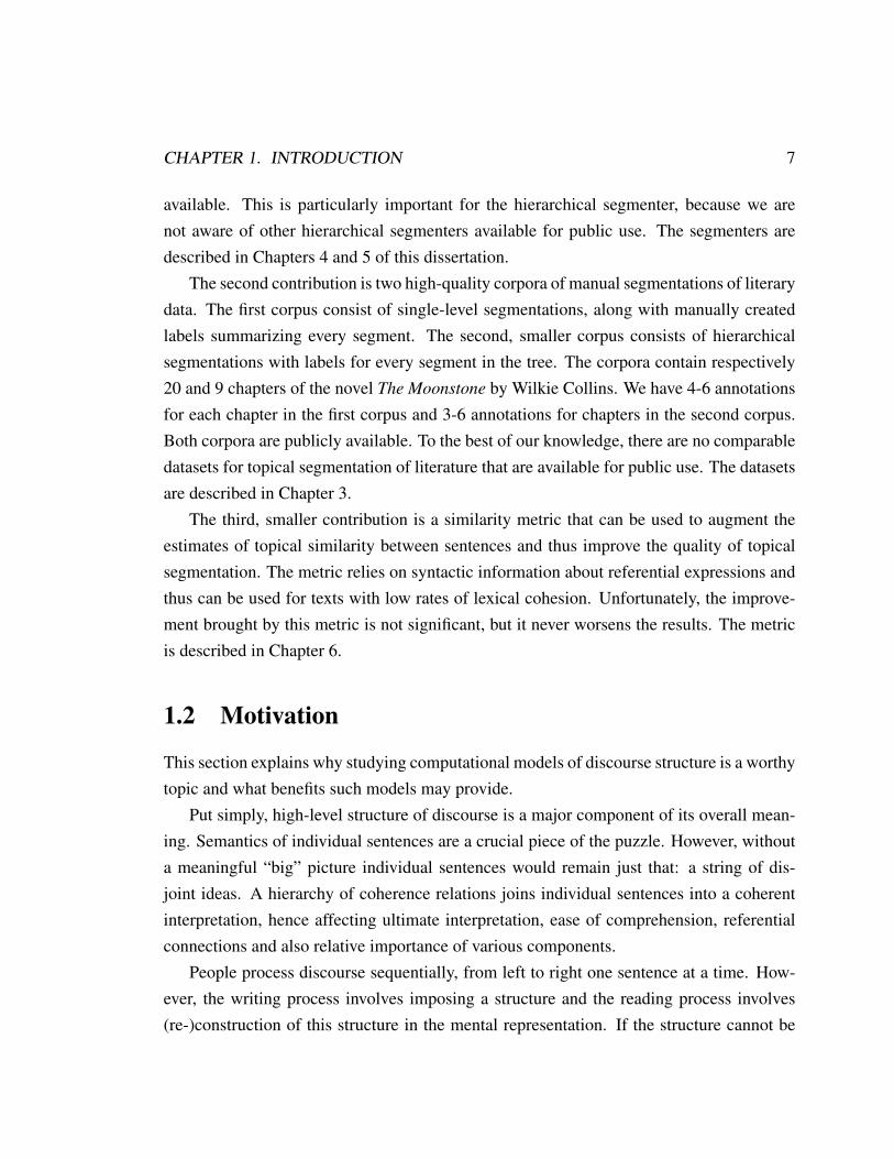
3.1.1 Overview . . . . . . . . . . . . . . . . . . . . . . . . . . . . . . . 443.1.2 Corpus description . . . . . . . . . . . . . . . . . . . . . . . . . . 453.1.3 Corpus analysis . . . . . . . . . . . . . . . . . . . . . . . . . . . . 463.1.4 Inter-annotator agreement . . . . . . . . . . . . . . . . . . . . . . 483.1.5 Patterns of disagreement . . . . . . . . . . . . . . . . . . . . . . . 523.1.6 Flat moonstone dataset: conclusions . . . . . . . . . . . . . . . . . 54
3.2 The Moonstone dataset 2: a dataset for hierarchical segmentation . . . . . . 553.2.1 Overview of the hierarchical dataset . . . . . . . . . . . . . . . . . 553.2.2 Hierarchical moonstone dataset: corpus overview . . . . . . . . . . 563.2.3 Hierarchical dataset: corpus analysis . . . . . . . . . . . . . . . . . 643.2.4 Conclusions about the hierarchical dataset . . . . . . . . . . . . . . 68
3.3 Conclusions . . . . . . . . . . . . . . . . . . . . . . . . . . . . . . . . . . 70
4 Affinity Propagation for text segmentation 714.1 Background: factor graphs and affinity propagation for clustering . . . . . . 74
4.1.1 Factor graphs and the max-sum algorithm . . . . . . . . . . . . . . 744.1.2 Affinity Propagation for clustering . . . . . . . . . . . . . . . . . . 75
4.2 Affinity Propagation for flat segmentation . . . . . . . . . . . . . . . . . . 784.3 Experimental settings . . . . . . . . . . . . . . . . . . . . . . . . . . . . . 864.4 Experimental results and discussion . . . . . . . . . . . . . . . . . . . . . 904.5 Conclusions . . . . . . . . . . . . . . . . . . . . . . . . . . . . . . . . . . 92
5 Hierarchical segmentation 955.1 Introduction . . . . . . . . . . . . . . . . . . . . . . . . . . . . . . . . . . 955.2 Formulating hierarchical Affinity Propagation for segmentation (HAPS) . . 98
5.2.1 Update messages for HAPS . . . . . . . . . . . . . . . . . . . . . 1035.3 Experimental setting . . . . . . . . . . . . . . . . . . . . . . . . . . . . . 1165.4 Experimental results and discussion . . . . . . . . . . . . . . . . . . . . . 124

CONTENTS vi
5.5 Evaluating informativeness of the segment centres . . . . . . . . . . . . . . 1265.6 Conclusions . . . . . . . . . . . . . . . . . . . . . . . . . . . . . . . . . . 128
6 Coreferential similarity 1316.1 Introduction . . . . . . . . . . . . . . . . . . . . . . . . . . . . . . . . . . 1316.2 Background: accessibility of antecedents and coreferential distance . . . . 1356.3 Estimating coreferential similarity . . . . . . . . . . . . . . . . . . . . . . 1396.4 Experimental evaluation . . . . . . . . . . . . . . . . . . . . . . . . . . . 1436.5 Experimental results and discussion . . . . . . . . . . . . . . . . . . . . . 1466.6 Conclusions . . . . . . . . . . . . . . . . . . . . . . . . . . . . . . . . . . 148
7 Conclusions and future work 1507.1 Contributions . . . . . . . . . . . . . . . . . . . . . . . . . . . . . . . . . 1507.2 Directions for future work . . . . . . . . . . . . . . . . . . . . . . . . . . 153
Bibliography 156
A Full text of Chapter II of The Moonstone 174
B Instructions for the flat segmentation experiment 179
C Weights used in the experiments with coreferential similarity 187

List of Figures
1.1 Jabberwocky by Lewis Carroll . . . . . . . . . . . . . . . . . . . . . . . . 21.2 Example segmentation of Chapter 2 of The Moonstone by Wilkie Collins.
Annotator 2. . . . . . . . . . . . . . . . . . . . . . . . . . . . . . . . . . . 41.3 Example of a topical tree for Chapter 2 of The Moonstone by Wilkie Collins. 5
2.1 Example plot-unit representation for the following toy story from [Lehnert,1982, p. 389]. John and Bill were competing for the same job promotion atIBM. John got the promotion and Bill decided to start his own consultingfirm, COMSYS. Within three years COMSYS was flourishing. By thattime John had become dissatisfied with IBM so he asked Bill for a job. Billspitefully turned him down. . . . . . . . . . . . . . . . . . . . . . . . . . 26
2.2 An example of a social network extracted from Jane Austen’s Mansfield
Park. From [Elson, 2012, p.36] . . . . . . . . . . . . . . . . . . . . . . . . 282.3 An example of an RST-tree from [Mann and Thompson, 1987, p.51] 1. One
difficulty is with sleeping bags in which down and feather fillers are usedas insulation. 2. This insulation has a tendency to slip towards the bottom.3. You can redistribute the filler 4. . . . 11. . . . . . . . . . . . . . . . . . . 31
2.4 Example segmentation for Chapter 2 of The Moonstone by Wilkie Collins.Annotator 2. . . . . . . . . . . . . . . . . . . . . . . . . . . . . . . . . . . 35
2.5 Topical tree for the segmentation. . . . . . . . . . . . . . . . . . . . . . . . 36
3.1 Distribution of segment counts across chapters. . . . . . . . . . . . . . . . 473.2 Annotator quality. . . . . . . . . . . . . . . . . . . . . . . . . . . . . . . . 483.3 Example segmentation for Chapter 1. . . . . . . . . . . . . . . . . . . . . 52
vii

LIST OF FIGURES viii
3.4 Quality of segment boundaries. . . . . . . . . . . . . . . . . . . . . . . . . 533.5 An example of hierarchical segmentation for Chapter 2. (Produced by An-
notator 1). . . . . . . . . . . . . . . . . . . . . . . . . . . . . . . . . . . . 573.6 Example segmentation for Chapter 2. Annotator 2. . . . . . . . . . . . . . 593.7 Example hierarchical segmentations for Chapter 2. . . . . . . . . . . . . . 613.8 Flattened representations of topical trees. . . . . . . . . . . . . . . . . . . 633.9 windowDiff values across levels of hierarchical segmentations. . . . . . . . 663.10 Mean pairwise S values for all annotators. . . . . . . . . . . . . . . . . . . 673.11 S-based inter-annotator agreement per chapter. . . . . . . . . . . . . . . . 683.12 Edit operations when computing S. Number of edits / chapter length * num-
ber of annotations . . . . . . . . . . . . . . . . . . . . . . . . . . . . . . . 69
4.1 Factor graph for F (x1, x2, x3, x4) = f1(x1, x2, x3) + f2(x2, x3, x4). . . . . . 754.2 Factor graph for affinity propagation. . . . . . . . . . . . . . . . . . . . . . 764.3 Example of valid configuration of hidden variables {cij} for clustering. . . 794.4 Example of valid configuration of hidden variables {cij} for segmentation. . 794.5 Example of flat segmentation of Chapter 2 of The Moonstone by Wilkie
Collins. Annotator 2. . . . . . . . . . . . . . . . . . . . . . . . . . . . . . 934.6 Segment centres identified by APS for Chapter 2 of The Moonstone by
Wilkie Collins. . . . . . . . . . . . . . . . . . . . . . . . . . . . . . . . . 93
5.1 Example of a topical tree for Chapter 2 of The Moonstone by Wilkie Collins. 965.2 Example segmentation of Chapter 2 of The Moonstone by Wilkie Collins.
Annotator 2. . . . . . . . . . . . . . . . . . . . . . . . . . . . . . . . . . . 975.3 Factor graph for Hierarchical Affinity Propagation for Segmentation, HAPS. 995.4 Message types sent in the HAPS model. . . . . . . . . . . . . . . . . . . . 1045.5 Example topical tree produced by HAPS for Chapter 2 of The Moonstone.
Two top levels. . . . . . . . . . . . . . . . . . . . . . . . . . . . . . . . . 122
6.1 An excerpt from The Moonstone, Chapter 5. . . . . . . . . . . . . . . . . . 1326.2 An excerpt from The Moonstone, Chapter 5 with all references to Colonel
John Herncastle made replaced by Colonel John Herncastle. . . . . . . . . 133

LIST OF FIGURES ix
6.3 A fragment of Samuel Beckett’s play Waiting for Godot (the focal entity,Godot, is mentioned explicitly only once) . . . . . . . . . . . . . . . . . . 137
6.4 Linguistic coding devices which signal topic accessibility Givon [1981] . . 1386.5 Categories of noun phrases taken into account when computing coreferen-
tial similarity . . . . . . . . . . . . . . . . . . . . . . . . . . . . . . . . . 1406.6 An example of computing coreferential similarity . . . . . . . . . . . . . . 142
List of Tables
3.1 Overview of inter-annotator agreement. . . . . . . . . . . . . . . . . . . . 513.2 Chapter assignments per groups of annotators. . . . . . . . . . . . . . . . . 653.3 Average breadth of the trees at different levels. . . . . . . . . . . . . . . . . 65
4.1 windowDiff values for the segmentations of the three datasets using theBayesian segmenter, the Minimum Cut segmenter and APS. The valuesin parentheses are standard deviations across all folds. . . . . . . . . . . . . 91
4.2 S values for the segmentations of the three datasets using the Bayesiansegmenter, the Minimum Cut segmenter and APS. . . . . . . . . . . . . . . 92
5.1 Evaluation of HAPS and iterative versions of Minimum Cut Segmenter andBayesian Segmenter using windowDiff per level and evalHDS . . . . . . . 124
5.2 Evaluation of HAPS and iterative version of Minimum Cut Segmenter usingSTS-2012 matrices as input. The table reports windowDiff per level andevalHDS and standard deviation. . . . . . . . . . . . . . . . . . . . . . . . 125
5.3 HAPS segment centres compared to CohSum summaries: ROUGE scoresand 95% confidence intervals . . . . . . . . . . . . . . . . . . . . . . . . . 128
6.1 Results of comparing APS and Minimum Cut Segmenter using four differ-ent matrix types (windowDiff values and standard deviation) . . . . . . . . 146
6.2 Results of comparing HAPS and hierarchical iterative version of the Mini-
mum Cut Segmenter using four different matrix types (evalHDS values andstandard deviation) . . . . . . . . . . . . . . . . . . . . . . . . . . . . . . 147
x

Chapter 1
Introduction
1.1 Overview
’Twas brillig, and the slithy tovesDid gyre and gimble in the wabe;
All mimsy were the borogoves,And the mome raths outgrabe.
“Beware the Jabberwock, my sonThe jaws that bite, the claws that catch!
Beware the Jubjub bird, and shunThe frumious Bandersnatch!”
He took his vorpal sword in hand;Long time the manxome foe he sought–
So rested he by the Tumtum tree,And stood awhile in thought.
And, as in uffish thought he stood,The Jabberwock, with eyes of flame,
Came whiffling through the tulgey wood,And burbled as it came!
1

CHAPTER 1. INTRODUCTION 2
One, two! One, two! And through and throughThe vorpal blade went snicker-snack!
He left it dead, and with its headHe went galumphing back.
“And hast thou slain the Jabberwock?Come to my arms, my beamish boy!
O frabjous day! Callooh! Callay!”He chortled in his joy.
’Twas brillig, and the slithy tovesDid gyre and gimble in the wabe;
All mimsy were the borogoves,And the mome raths outgrabe.
Figure 1.1: Jabberwocky by Lewis Carroll
Lewis Carroll’s famous poem is an example of nonsense verse – a light genre of poetryusually read to children, which does not make sense in the context of what we know aboutthe world. It cannot be fully processed semantically because the reader does not know whoJabberwock is, or why one should be afraid of Bandersnatch. This, however, presents littleproblem for children, to whom a dentist is no less mysterious (or frightening) a creature.The poem contains enough syntactic, morphological and temporal information for a readerto flesh out an interpretation, even with missing variables. Without creating a full interpre-tation, the reader can easily understand the initial idyllic setting with slithy toves gimblingin the wabe, then the warning a son receives, his battle with the Jabberwock, the parent’sjoy and eventually the return to the initial setting.
This particular example contains quite a bit of regular lexemes to aid the understand-ing. However, a lot of burden also falls on structural devices: conjunctions that mark thesyntactic structure of the sentences, commas, exclamation marks, markers of direct speech,shifting in tense and verbal aspect and, of course, the traditional shape of the 19th cen-tury English poem. While lacking in lexical semantics, the poem can be read and enjoyedbecause its structure is familiar and interpretable.
People leverage the knowledge about the structure of discourse quite heavily, both interms of its comprehension and its creation. It is useful in conversations and institutional
CHAPTER 1. INTRODUCTION 3
rhetoric [van Dijk, 2007, Jacobs and van Hout, 2009, Rocci, 2009]. It has been shown toaffect how people summarize and recall information [Endres-Niggemeyer, 1998]. Peoplestructure their writing according to expectations for a particular genre as well as buildingan argument so as to convey the desired message [Jacobs and van Hout, 2009].
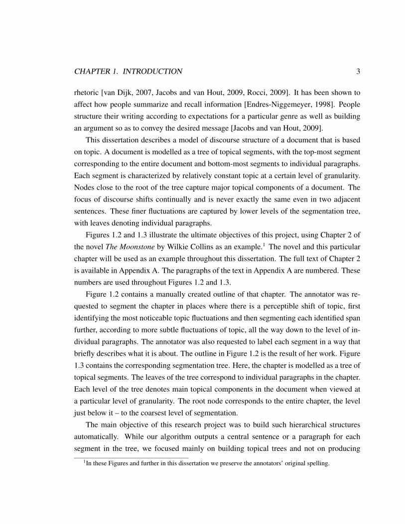
This dissertation describes a model of discourse structure of a document that is basedon topic. A document is modelled as a tree of topical segments, with the top-most segmentcorresponding to the entire document and bottom-most segments to individual paragraphs.Each segment is characterized by relatively constant topic at a certain level of granularity.Nodes close to the root of the tree capture major topical components of a document. Thefocus of discourse shifts continually and is never exactly the same even in two adjacentsentences. These finer fluctuations are captured by lower levels of the segmentation tree,with leaves denoting individual paragraphs.
Figures 1.2 and 1.3 illustrate the ultimate objectives of this project, using Chapter 2 ofthe novel The Moonstone by Wilkie Collins as an example.1 The novel and this particularchapter will be used as an example throughout this dissertation. The full text of Chapter 2is available in Appendix A. The paragraphs of the text in Appendix A are numbered. Thesenumbers are used throughout Figures 1.2 and 1.3.
Figure 1.2 contains a manually created outline of that chapter. The annotator was re-quested to segment the chapter in places where there is a perceptible shift of topic, firstidentifying the most noticeable topic fluctuations and then segmenting each identified spanfurther, according to more subtle fluctuations of topic, all the way down to the level of in-dividual paragraphs. The annotator was also requested to label each segment in a way thatbriefly describes what it is about. The outline in Figure 1.2 is the result of her work. Figure1.3 contains the corresponding segmentation tree. Here, the chapter is modelled as a tree oftopical segments. The leaves of the tree correspond to individual paragraphs in the chapter.Each level of the tree denotes main topical components in the document when viewed ata particular level of granularity. The root node corresponds to the entire chapter, the leveljust below it – to the coarsest level of segmentation.
The main objective of this research project was to build such hierarchical structuresautomatically. While our algorithm outputs a central sentence or a paragraph for eachsegment in the tree, we focused mainly on building topical trees and not on producing
1In these Figures and further in this dissertation we preserve the annotators’ original spelling.

CHAPTER 1. INTRODUCTION 4
Figure 1.2: Example segmentation of Chapter 2 of The Moonstone by Wilkie Collins.Annotator 2.
1. Paragraphs 1-4: the single life of the narrator (a note: paragraph one sets the time thestory begins)
(a) paragraph 1: the diamond’s location
(b) paragraphs 2-4: how he came to be in his career
i. paragraph 2: how he met the ladyii. paragraph 3: how he became hired by the lady
iii. how he came to be promoted to bailiff
2. paragraphs 5-10: life with a love interest before and after marriage
(a) paragraphs 5-8: motivations for finding a wife
i. paragraph 5: lonelinessii. paragraph 6: economics and love
iii. paragraphs 7-8: the lady’s approvalA. paragraph 7: asking for approvalB. paragraph 8: receiving approval
(b) paragraphs 9-10: experiences of marrying and being married to a woman
i. paragraph 9: apprehensions about marriageii. paragraph 10: mediocrity in married life
3. paragraphs 11-15: life as a widower and into old age
(a) paragraph 11: death of the narrator’s wife and first mention of daughter Penelope
(b) paragraphs 12-14: convincing the narrator to alter his occupation
i. paragraph 12: Lady lulls him into security with kindnessii. paragraph 13: narrator realises her plan, and his pride fights against it
iii. paragraph 14: narrator is convinced after reading Crusoe he will feel betterabout it tomorrow
(c) paragraph 15: the difficulty of writing a story without accidentally writing aboutoneself (a note: only technically in his old age, not really about his old age)

CHAPTER 1. INTRODUCTION 5
Figure 1.3: Example of a topical tree for Chapter 2 of The Moonstone by WilkieCollins.
coherent labels for each segment. That is why the result is more like the tree in Figure 1.3,not the complete outline in Figure 1.2. Performing the segmentation on its own is difficultenough. In order to find the appropriate labels, we would need to summarize each segmentreasonably well and to either extract or generate an appropriate label. Quite often, but notalways, the segment centres provide an adequate summary of the segment. At this stage,we made no effort to generate good labels for the nodes in the topical trees.
The main reasons for modelling discourse structure in this manner are computationalfeasibility and applicability. Topic is defined as a set of entities under discussion [Webberet al., 2012, p. 440]. This definition is rather loose and it is not always possible to providea more precise view. The definition becomes task-dependent in that it depends on whatthe final goal of segmentation is [Purver, 2011, p. 292]. In fiction, as the topic changes,the shift is often accompanied by other changes in structure: the narrator may shift, adialogue may end, the tempo of narration may change, etc. Therefore, a topical tree inFigure 1.3 collapses several paradigms into one representation. It subsumes informationabout temporal structure of the narrative, about dialogue-act structure, about presentationaland other types of discourse relations.
Yet, there are several reasons why we feel this is an adequate representation. Mainly,it is a viable trade-off between usefulness and feasibility. Modelling a novel as a topical

CHAPTER 1. INTRODUCTION 6
tree creates a structure that says something about the main themes in the novel. For manygeneric NLP applications, the theme, or “aboutness”, is of high relevance. One such ap-plication is generic automatic summarization, which deals with finding the crucial piecesof information capturing what the document is about. It has been shown that the knowl-edge of discourse structure can be helpful in summarizing documents, e.g., [Uzeda et al.,2010]. However, automatically determining detailed information about discourse structureis a challenging problem (see Section 2.3 for a review). Topical trees are a useful, if lessinformative, alternative. To date, models based on topical segments have been used ininformation extraction, essay analysis and scoring, automatic assessment of coherence oftext, automatic dialogue systems, etc. [Webber et al., 2012]. On the other side of the issueis computational feasibility. There is a number of detailed and well-researched theoriesof discourse structure and of narrative structure (see Chapter 2 for a detailed review), yetmost of them are described in terms too abstract to be useful for computational modelling,or they do not scale well to such large documents as novels. That is why we decided tochoose a simple but useful representation that can be constructed relatively easily.
The model proposed here is suitable for most expository and narrative types of dis-course. While we use certain devices to alleviate the problem of low lexical repetition infiction (see Chapter 6), overall the methods we use are applicable to any data type. Thesoftware would need to be fine-tuned and it may work better or worse depending on thegenre and on the ultimate objectives. For example, one would expect poorer performanceon dialogues, or in situations where the desired segmentations may not correspond to shiftsof topic.
The particular implementations described in this proposal are geared towards literarydata, especially novels. However, we test our tools on several benchmark datasets thatcontain data of different genres, namely speech transcripts, chapters of medical textbooksand Wikipedia articles.
Contributions. We hope that this work contributes something to the field of automaticdiscourse analysis as well as to research on creating tools for processing literature. In ourview, there are several key contributions.
The first and possibly most important contributions are the two algorithms for topicalsegmentation of documents – one for building flat structures and another for producingtopical trees of any desired depth. Both have been implemented in Java and are publicly
CHAPTER 1. INTRODUCTION 7
available. This is particularly important for the hierarchical segmenter, because we arenot aware of other hierarchical segmenters available for public use. The segmenters aredescribed in Chapters 4 and 5 of this dissertation.
The second contribution is two high-quality corpora of manual segmentations of literarydata. The first corpus consist of single-level segmentations, along with manually createdlabels summarizing every segment. The second, smaller corpus consists of hierarchicalsegmentations with labels for every segment in the tree. The corpora contain respectively20 and 9 chapters of the novel The Moonstone by Wilkie Collins. We have 4-6 annotationsfor each chapter in the first corpus and 3-6 annotations for chapters in the second corpus.Both corpora are publicly available. To the best of our knowledge, there are no comparabledatasets for topical segmentation of literature that are available for public use. The datasetsare described in Chapter 3.
The third, smaller contribution is a similarity metric that can be used to augment theestimates of topical similarity between sentences and thus improve the quality of topicalsegmentation. The metric relies on syntactic information about referential expressions andthus can be used for texts with low rates of lexical cohesion. Unfortunately, the improve-ment brought by this metric is not significant, but it never worsens the results. The metricis described in Chapter 6.
1.2 Motivation
This section explains why studying computational models of discourse structure is a worthytopic and what benefits such models may provide.
Put simply, high-level structure of discourse is a major component of its overall mean-ing. Semantics of individual sentences are a crucial piece of the puzzle. However, withouta meaningful “big” picture individual sentences would remain just that: a string of dis-joint ideas. A hierarchy of coherence relations joins individual sentences into a coherentinterpretation, hence affecting ultimate interpretation, ease of comprehension, referentialconnections and also relative importance of various components.
People process discourse sequentially, from left to right one sentence at a time. How-ever, the writing process involves imposing a structure and the reading process involves(re-)construction of this structure in the mental representation. If the structure cannot be

CHAPTER 1. INTRODUCTION 8
re-created, then we call such discourse incoherent: individual items make sense, but thereis no overall meaning to a document.
Ultimately, in the field of Natural Language Processing we are concerned with extract-ing and utilizing meaning in various ways. In text summarization, we want to find meaningand express it as briefly as possible; in machine translation, we are concerned with re-wording meaning in a different language; in question answering, we are concerned withfinding a specific piece of meaning, etc. That is why we think that studying computationalmodels of discourse structure is a worthy endeavour – because it is (most likely) necessaryto adequately extract and represent the meaning of documents.
None of the aforementioned statements are novel. Young and Becker [1966] haveshown that coherent discourse cannot be constructed one sentence at a time. It is alsowell known that discourse is more than a sequence of unconstrained sentences [Renkema,2004, pp. 35-50]. Kehler [2002] has shown that discourse relations influence the inter-pretation and construction of referential expressions, verb ellipsis, gapping and tense; alsosee [Renkema, 2004, pp. 87-120]. However, Computational Linguistics has been some-what slow to put this knowledge to use, if not to recognize its importance in theory. Inthe past 20 years, part-of-speech tagging, syntactic parsing, anaphora resolution and someother intermediate applications have become reliable and indispensable tools. Of course,quite a number of people have worked on robust discourse parsing, but to the best of ourknowledge, there are no publicly available robust discourse parsers (see Section 2.3 for areview of relevant related work). What is more important, there is no strong theory of howto make use of them for other NLP tasks, such as machine translation, automatic summa-rization, question answering etc.
This is particularly the case for text genres that lack rigid structure: blogs, e-mails,speech transcripts, literature. The few existing tools perform quite poorly on these data,where they would be most useful. This is a pity because, while it is possible to knowsomething about the structure of a scientific paper a priori and to encode it manually, itis practically impossible to create such templates for blogs, meeting transcripts and mostliterary data.
Given all the fascinating dependencies between discourse structure and other linguisticphenomena, it seems that making even a small step in this direction would be beneficial.Modelling discourse structure as a tree of topical segments is a far cry from building a tree

CHAPTER 1. INTRODUCTION 9
of coherence relations (see Section 2.3 for a review). This representation certainly containsless information, yet it is feasible to build it for a large document, such as a novel.
1.3 Overview
Put simply, in this research, a document is modelled as a tree of segments, each focusedon a particular topic. The root of the tree is the complete document. Nodes close to theroot correspond to large segments of text; topic shifts between high-level segments arenoticeable and rather abrupt. Nodes further down in the tree model finer fluctuations ofthe topic. A manually constructed topic tree for Chapter 2 of The Moonstone is shown inFigure 1.3.
In this work, we explore two main points:
1. An efficient algorithm for flat and hierarchical text segmentation. We use factorgraphs as a framework for hierarchical text segmentation. The proposed algorithm isan adaptation of a recent clustering algorithm, Affinity Propagation [Frey and Dueck,2007]. Given a sequence of sentences (or paragraphs), the algorithm outputs segmentboundaries and segment centres – points that best describe what the segment is about.We derive and implement two topical segmenters based on Affinity Propagation: aflat segmenter and a hierarchical one.
2. A similarity measure that helps detect topic fluctuations in running text. It was al-ready mentioned that this work is concerned with informal documents and mostlywith literature. In such documents the rate of lexical repetition is much lower than informal texts [Hoey, 1991, Graesser et al., 2004, Louwerse et al., 2004]. That is whywe develop a syntactically motivated measure for tracking topic changes betweensentences. The basis for this metric is the theory of functional domains developed byTalmy Givon (1981). According to Givon, the accessibility of concepts mentionedin text is in inverse relation with how much information the author needs to specifyin order to (re)introduce a concept. Concepts mentioned most recently will requirethe least amount of coding and can be expressed by pronominal or zero anaphora.Concepts that are more difficult to access must be invoked explicitly (e.g., using a

CHAPTER 1. INTRODUCTION 10
proper noun). If they are even less accessible, invoking them will require pre- orpost-modification (to remind the reader what they are).
1.4 Justification of the proposed method
1.4.1 Reasons for using topical segmentation
Modelling novels as trees of topical segments is certainly not the only way to go aboutmodelling discourse structure. A large body of research in philosophy, narratology andliterary studies describes regularities in literature from different angles (see Section 2.1for a review). Some researchers have tried to model literary narratives computationally(Section 2.2). There is also a lot of research that deals with how form and function arelinked in discourse in general (Section 2.3). Why did we choose topical segmentation asthe model of choice?
There are several reasons. They are explained in more detail in Chapter 2 which pro-vides the context for comparisons, but we outline them here briefly.
The main issue with non-computational models of narratives is that they are expressedin terms which do not lend themselves easily to algorithmization. While it makes sense toview a book as consisting of a message (fabula), an event structure (story) and the actualtext, this is hardly helpful computationally, since it is very challenging to build a model ofevent structure for even a toy story, let along get at the core message it is meant to convey.Section 2.1 provides a review of relevant non-computational models. None of them can beapplied computationally with any reasonable reliability.
Section 2.2 describes recent work in computational narratology which builds upon tra-ditional narratology, as well as offers its own insight into how narratives can be modelledcomputationally. While this area has witnessed rapid growth lately, most approaches wouldalso not scale easily to novels. Additionally, to verify their applicability one would needto create a corpus annotated according to the specifications of a model. Since such modelsare rather detailed, it would be prohibitively expensive and time-consuming to annotate awork as large as a novel.
We also decided against using existing research on generic approaches to modellingdiscourse structure (Section 2.3). Issues of scalability and creating a corpus of fine-grained

CHAPTER 1. INTRODUCTION 11
annotations are seen here again. Additionally, existing models of discourse structure, e.g.,
RST [Mann and Thompson, 1987], were developed for expository texts and it is far fromobvious how to apply them to literary data. Literature is full of metaphors, dialogues,criss-crossing topical threads, etc. While it is possible to think of extensions, it is neitherstraight-forward nor guaranteed to be useful computationally.
We decided to use topical segmentation because, despite not being the most informativeor detailed model, it is likely to be useful and it can be computed relatively easily giventhe state-of-the-art in NLP. It is also simple enough cognitively to allow the creation of abenchmark corpus to test our hypotheses.
1.4.2 Reasons for using a syntactically motivated similarity measure
Most available segmenters rely only on word repetition to model topic in discourse. Givenhow well-studied measures of text similarity and relatedness are, this is far from being themost informative metric. Some research on text segmentation also uses dictionary-basedand corpus-based similarity metrics, but none of the publicly available segmenters offersuch options (see Section 6.2 for review of related work).
However, lexical cohesion (and synonymy is one of the devices of lexical cohesion) isgenerally lower for texts that are cognitively simple to process. In other words, the simplerthe topic at hand is, the less need there is for the author to explicitly code what he is talkingabout. Therefore, any similarity metric that relies only on lexical information will have arather low upper limit on texts that are prevalent in real life: non-scientific books, personalcorrespondence, speech transcripts.
That is why in this work we propose a similarity metric that uses syntactic informationabout referential expressions in text. It does not improve the results as much as we wouldlike it to, but it does offer a small improvement.
1.5 Organization
This dissertation is structured as follows. Chapter 2 provides an overview of research onautomatic modelling of discourse structure in general and on modelling literary narrativesin particular. Chapter 3 explains how we plan to evaluate our progress and describes in

CHAPTER 1. INTRODUCTION 12
detail the two datasets that we have created for the purposes of studying topical structure ofnarratives and for the evaluation of our system. Chapter 4 describes the part of the systemdeveloped thus far and how it compares with the state-of-the-art. Chapter 6 outlines asyntactically-motivated measure of topical similarity. Chapter 7 concludes this dissertationby discussing the results of this work, possible improvements and outlining our plans forfuture work.
1.6 Conclusion
This work is concerned with modelling discourse structure of literature, mainly novels.We chose to model structure using topical trees, which capture fluctuations of topic. Thisway to model structure is not specific to literature, yet we chose it for several reason. Ina situation where there is no theoretical framework that can be applied computationally(see next chapter for a comparative review of alternative approaches), topical segmentationprovides a light-weight method. Topical trees can be computed with relative ease andencouraging performance. They capture the notion of topic in a way that can be useful forother applications, as we hope to demonstrate in future work.
The main contributions of this work are the algorithms and the software for single-leveland hierarchical topical segmentation, and the corpora of manual segmentation for a partof the novel The Moonstone.
Topical trees are not specific to literature. They can be built for almost any genre. Infact, in this dissertation we also build them for Wikipedia articles. Similarly, the syntactically-motivated similarity metric outlined in Chapter 6 is also not specific to literature and canhopefully be useful for any coherent text with low rates of lexical repetition. However, themethods used in this work are chosen first and foremost so as to work on literature. Wealso would like our methods to scale to large corpora of literature and to be fast, light andnot require excessive amounts of human labor. If they are applicable to other genres oftext (e.g., speech), so much the better. Yet, our main interest and focus is literature. Thestatistical nature of our methods reflects a trade-off between what needs to be done andwhat can feasibly be done – for now, of course.

CHAPTER 1. INTRODUCTION 13
1.6.1 Previous publications
Parts of chapters 3 and 4 have been published in [Kazantseva and Szpakowicz, 2011, 2012].Parts of chapters 5 and 6 have been published in [Kazantseva and Szpakowicz, 2014a,b].

Chapter 2
Related work
This work focuses on modelling the structure of long literary narratives, mostly novels.This question has not been studied in depth by the community of Natural Language Pro-cessing researchers. However, relevant aspects of it have been well explored in severalfields.
When attempting to model the structure of novels computationally, one is naturallyinclined to look into literary theories of novels. Narratologists and literary critics have beenasking questions about main elements of novels, trends, tendencies and laws of literaturefor many centuries. It is a vastly diverse body of work most of which, unfortunately, isoutlined in terms too abstract to be applicable computationally. However, in Section 2.1 webriefly review a few relevant theories of literary narrative.
Another highly relevant body of research is what we loosely term computational narra-
tology. Under this broad umbrella, we place research on the structure and interpretation ofstories (or, more generally, narratives) by people who are eventually interested in applyingtheir theories computationally. Research on story understanding was a popular topic in theAI community during the 1970s and 1980s (e.g., [Cullingford, 1978, Dyer, 1983]). Morerecently, it has been picked up with a somewhat different emphasis in the area of DigitalHumanities and a growing community of researchers explicitly working on computationalmodels of narratives. Many of these theories are highly relevant and in fact very promising.However, most of them have been developed for short narratives and cannot yet be ap-plied to novels with acceptable accuracy. Section 2.2 reviews the approaches to modellingnarratives computationally.
14

CHAPTER 2. RELATED WORK 15
Yet another point of view comes from the community of computational linguists work-ing on discourse structure. There is a number of well-developed and tested theories of howsmall units of discourse (for example, sentences) combine into larger semantic units, howthe combined meaning can be composed and how the process can be modelled computa-tionally. With a fair number of researchers working in this area, an ACM special interestgroup (Special Interest Group on Discourse and Dialogue (SIGDial)) and several annualworkshops, there has been a lot of progress. However, several aspects of this researchmade us decide against using existing theories of discourse structure to model novels. Firstof all, from the theoretical point of view, these theories have been developed for expositorytext and lack explanatory power for narratives (for example, temporal relations or relationsbetween various characters). Secondly, it is far from obvious how these theories can scaleto large texts such as novels (or even short stories), since they have been developed andexplained on relatively short expository texts. Section 2.3 provides a brief overview of thiswork and how it relates to the research proposed here.
Section 2.4 provides a brief overview of related work on text segmentation, directlyexplaining what has been done in the area of modelling discourse using methods such aswe propose here.
In Section 2.6, we explain why we chose to pursue the proposed method in the contextof what is already known and/or computable for long literary narratives.
2.1 Elements of literary narrative from the perspective ofliterary theory and narratology
Narrative fiction is defined as narration of a succession of fictional events [Rimmon-Kenan,1983, p.3]. It is generally agreed upon that a work of literature (or, more generally, a story)has several levels of abstraction:
1. The text: the actual discourse that tells the story. It is the only part immediatelyavailable to the reader.
2. The narration: the act of production or the telling of the story.
3. The story: the series of events, abstracted from their disposition in text.

CHAPTER 2. RELATED WORK 16
This classification is due to Rimmon-Kenan [1983, p.3]. Similarly, Bal [1985, p.5-10]distinguishes between the text (the actual words that tell the story), the fabula (a seriesof events experienced by the actors) and the story (a subset of the events from the fabulachosen to convey the message of the story). There are other similar classifications (e.g.[Propp, 1968, Greimas, 1971]) that distinguish layers of meaning in the story based onwhat the message is as opposed to how it is expressed.
Many have expressed the idea that at a certain level stories share common elements andthe variety of the stories in the cultural heritage is due to the variety of ways these elementscan be combined, not to the infinite variety of elements. The idea has been pioneered in1928 by Vladimir Propp [1968] who manually analyzed one hundred Russian folk talesand proposed that they consist of functions – low level cognitive elements of the plot.Examples of these functions are Absentation (a hero leaves home), Interdiction (a heroreceives a warning not to perform certain actions or go a certain way), Trickery (a villainattempts to deceive the hero), etc. Propp postulated that the order of these functions isrestricted even if not all of them are present in every story. The idea was further advancedand built upon by the structuralists in Prague and in France. Claude Levi-Strauss [1955]proposed that underlying the stories of a given culture are atomic units called mythemes.Mythemes are combined together to form the discourse of the myths. Barthes [1970] isanother philosopher who attempted to cast narrative discourse as a sequence of surfaceunits stemming from an underlying narrative grammar.
These theories had an enormous influence on the AI community during the 1970s andthe 1980s (see Section 2.2 for details). While there is no universally accepted narrativegrammar available today (much less one that could be used computationally), the idea ofviewing narrative discourse as a sequence of basic cognitive units has laid the foundationsfor the computational study of narratives as we know it today. However, several shortcom-ings make it very difficult to apply computationally. First of all, basic cognitive units suchas Propp’s function or Levi-Strauss’ mythemes are defined in a way that makes it difficultfor the-state-of-the art NLP technology to identify them in the actual textual discourse.Additionally, many have questioned the very essence of such an approach. Ryan [1991]points out that the number of possible actions that may be described in a story is probablyinfinite – as opposed to the number of terminals in any lexicon. Bod et al. [2012] questionhow objective Propp’s definitions of function are by demonstrating that his annotations are

CHAPTER 2. RELATED WORK 17
not trivial to reproduce. And, more broadly, more contemporary literary theory (e.g. Eco[1979]) emphasizes the active role of the reader in the interpretation of literature, suggest-ing that representing literature as a sequence of pre-determined cognitive units may be toosimplistic.
2.1.1 Events in stories
We have defined the narrative as the sequence of events, thus suggesting that events are cen-tral elements of any story. Indeed, a story can be defined as a sequence of events governedby temporal and causal links.
In the previous section, we have made a distinction between the layers of meaning inthe story, separating what is being told from how it is being told. The importance of eventsin stories can hardly be underestimated. In terms of structural analysis, one of the layers ofmeaning, inevitably, is the events of the story abstracted from the language and, dependingon a specific theory, from particular details of the story. Propp’s functions are event-based,as are the basic units of the story structure proposed by Claude Bremond [1973].
Bal [1985, p.19-22] remarks that even though it is agreed upon that events are con-stituent units of the story, it is far from obvious which sentences specify events, as well weas which events should be included in the storyline. She suggests three main criteria fordefining what constitutes relevant events (also called functional events of the story). Thesecriteria are change, choice and confrontation. While not cast in stone, these rules suggestthat an event is a change of state in the story world, which opens a possibility that mayor may not be taken up by a character or the author. The third criterion refers to the ideathat interesting events in the story are usually those that revolve around a conflict betweenseveral characters or groups of characters.
If a story (or fabula, using Bal’s terms) is a sequence of events, how are these to becombined? There are two paramount principles of combination: temporal links and causal-ity.
While we may be inclined to think of temporal progression as the natural order ofevents, in reality, this scenario is almost never encountered in stories. If a story contains atleast two characters, events become concurrent, and the narrated timeline becomes jagged,possibly with flashbacks and digressions [Rimmon-Kenan, 1983, p.17].

CHAPTER 2. RELATED WORK 18
The second principle of combination of events is causality. Foster [1963, p.93] postu-lated that the difference between a story and a plot lies in causality.
1. The king died and then the queen died.
2. The king died and then the queen died of grief.
While the former is a story, the latter is a plot.1 Temporal and causal connections areoften closely related in stories and cannot be readily separated.
Events combine into sequences to form the fabula – or the storyline. Bremond [1973]defines stories in terms of narrative cycles – event-based constituents of the story struc-ture. Each cycle is viewed as either an improvement or a deterioration. By comparing thenarrative cycles it is possible to compare the stories structurally.
Barthes [1970] categorizes events into kernels and catalysts based on their function inthe story line. Kernels are events that open possibilities for plot development. Having beenoffered a university admission, a character may or may not accept it. Thus, this is a kernelevent. On the other hand, pacing the room, looking out the window while making up one’smind are examples of catalyst events – events that magnify or delay one of the kernels.
2.1.2 Characters in stories
The omni-presence of human or human-like agents in narrative discourse is quite indicativeof our fascination with our selves. The human mind is preoccupied with comprehending it-self, musing about our values, imperfections, limitations. It is fascinating that the narrative,as we know it, is always about some aspect of human nature, even if related indirectly. It hasbeen shown that people find stories to be more comprehensible when there are well-formedrelationships between character actions and recognizable character goals, e.g., [Graesseret al., 1994]. However, it is not clear whether characters should be looked upon as people,or template-like structures that can be reconstructed from words [Rimmon-Kenan, 1983,p.31].
1Foster defines a story as a sequence of events arranged in time. This definition is misaligned with thedefinition from the previous chapter where a story denotes a specific layer of meaning. In our terminology,Foster’s story is closer to narrative.

CHAPTER 2. RELATED WORK 19
Literary theory does not quite agree on whether characters supersede events or the otherway round. In the purist tradition, a character exists only insofar as it is a part of imagesand events conveyed by the author [Aristotle, 1961, Propp, 1968, Greimas, 1971]. In therealist tradition [Ferrara, 1974] characters are modelled after real people and eventuallythey acquire some degree of independence from the text.
It is possible to evaluate characters along the axes of complexity, development, pene-tration into inner life and other traits. The basic principles of character reconstruction fromthe text are repetition, similarity, contrast and implication.
A body of research in cognitive psychology also points to the importance that agentsand their goals have in story comprehension and recall. Heider and Simmel [1944], Dik andAarts [2007] showed that even when people are shown cartoons about inanimate objects,they comprehend them in terms of animate agents, their struggles and goals.
Not surprisingly, a considerable number of representations for modelling narratives isexpressed in terms of characters and their affective states. We will discuss formalizedmodels based on characters in Section 2.2.2.
2.1.3 Conclusions
This section offered a very brief overview of narratives and their main components fromthe point of view of literary theory and narratology. It is agreed upon that stories are multi-layered entities with different levels of abstraction and meaning, from the actual words tothe abstract message of the story. Some of the crucial elements of stories are the event andtemporal structure, the character networks and the goals and motivations of those charac-ters.
Literary theory and narratology are broad and diverse fields. Studying stories in termsof their characters and event structure are certainly not the only interesting forms of anal-yses. One may also look at stories in terms of their temporal structure, focalization point,style, etc. In this review, we have included only the aspects most relevant to computationalmodelling of narratives.
As we will see in Section 2.2, much of the terminology and agreed-upon knowledgeabout the structure of stories has been borrowed by computational narratologists. Muchof the analyses described in this section cannot be easily automated. For example, the

CHAPTER 2. RELATED WORK 20
structuralist approach seems very intuitive to computer scientists, but automatically identi-fying functions or mythemes in literature is not possible with the state of the art in NaturalLanguage Processing. Classifying micro-sequences of events into deteriorations and im-provements in the style of Claude Bremond would allow finding similarities across stories,but even precise identification of events is a challenging task, let along classifying eventsequences into positive and negative ones (although this is perhaps a more feasible taskthan finding mythemes automatically).
2.2 Computational approaches to modelling narratives
The theories of narratives outlined above (along with many more in-depth studies) haveinfluenced an interdisciplinary field known as computational narratology. Computationalnarratologists are concerned with studying the laws and regularities of the narratives us-ing computers and corpus-based methods, as well as how this knowledge can be used forautomatic generation of narratives.
The theories of Vladimir Propp and those of the structuralist school have had a seri-ous influence of the AI community during the 1970s and the 1980s. The idea that surfacestructure of a story (i.e., its text) is generated from an underlying grammar is very appeal-ing to the mind of a computer scientist. Additionally, simultaneous research in cognitivepsychology had shown that previous experience and knowledge affects perception of theworld. In the now well-known experiment, Brewer and Treyens [1981] have invited stu-dents to participate in an experiment where they were asked to describe the contents of aroom. The students were told they would need to wait in a colleague’s office while waitingfor the experiment to start. After a brief period of waiting, they were led to a different roomand asked to describe the contents of the previous office. The descriptions provided by thestudents contained items that one would expect to see in an office: books, notebooks, etc.Curiously, the students “saw” some office-like items that were not there and failed to noticeitems which are normally not found in offices.
BORIS [Dyer, 1983] is an example of a well-known story-understanding system fromthat period. The system is based on the assumption that common world knowledge abouttypical situations can be organized using scripts – general and somewhat stereotyped knowl-edge about a particular situation. A script about eating at a restaurant, for example, would

CHAPTER 2. RELATED WORK 21
“know” about menus, waiters, paying the bill, etc. A script about divorces would includeinformation about the two spouses, some conflict that led to the divorce, the knowledgethat before the divorce they lived together and that this will not continue to be so after thefact. BORIS processed stories word-by-word, invoking a rich semantic representation foreach lexeme, which was manually encoded in an elaborate lexicon. Additionally, it reliedon a manually encoded set of scripts which encoded common-sense knowledge about thesituations that BORIS was asked to process. BORIS was able to “understand” the stories it“knew” about and answer questions about them.
A story-understanding system with a slightly different flavour is PAM (Plan ApplicationMechanism) [Wilensky, 1977]. PAM’s understanding of stories is based on identifying theintentions of its characters and connecting all the events in the story by causal links in as faras they are related to characters’ goals. As PAM “read” a story, it produced a representationusing conceptual dependencies, linking them into a knowledge structure Interpretation.
A story-generation system that relied on hand-coded knowledge is UNIVERSE [Lebowitz,1983]. UNIVERSE was able to create brief stories, focusing on melodramatic interpersonalsituations, creating highly believable characters. UNIVERSE was organized around plans– those of the author and those of the characters. It had at its disposal a library of manuallyencoded plot fragments, which it combined to create interesting story-lines.
BORIS, PAM and UNIVERSE exemplify many of their contemporaries e.g., [Norvig,1989, Cullingford, 1978, Thorndyke, 1975]. Most of these systems suffered from a knowl-edge acquisition problem: while awing audiences with performance on familiar scripts,they were helpless in unfamiliar situations. Worse yet, extending such a system is apainstaking and a labor-intensive process. Several attempts have been made to circum-vent this problem [Norvig, 1983] or acquire the knowledge automatically [Chambers andJurafsky, 2009], but it largely remains an unresolved issue.
Later efforts have revolved around finding more abstract representations that wouldencode higher-level regularities in narratives and would not require so much manual effort.In the following two subsections, we will describe some of the representative approachesto modelling narratives computationally, roughly subdividing them into event-based andcharacter-based. However, it should be noted that this sub-division is somewhat illusory,as all of them model both aspects to some extent. (This is in line with the ongoing debatein narratology as to whether characters are subordinate to events or the other way round. )

CHAPTER 2. RELATED WORK 22
We placed them into one category or another depending on what is of primary importanceto a given representation.
2.2.1 Event-based approaches to modelling narratives
Aristotle considered the plot to be the soul of tragedy [Aristotle, 1961]. A fair numberof more contemporary formal representations of narratives are based on modelling mainevents in a story and how they are related causally or temporarily.
Trabasso and Sperry [1985], Trabasso and Stein [1997] model the process of narra-tive comprehension based on causality. The model, Recursive Transition Causal Networks(RTCNs), builds a representation consisting of the fragments of a story connected withcausal links. There are six classes of such fragments: Settings, Initiating Event, Reactions,Goals, Actions and Outcome of goals. There is a link between two nodes in the graph ifone event necessarily follows another, in the eyes of the reader. The model is primarily amodel of how humans process narrative discourse. It has been extensively used to studyinferences occurring during the reading process.
One possible way to represent narratives computationally (especially for the purposesof narrative generation) is by using plans. Planning allows building plot lines that are tem-porarily and causally sound. IPOCL (Intentional Partial Order Causal Link planner) [Riedland Young, 2010] is a story generation system built with two primary goals in mind: logi-cal causal progression of the plot and believable characters (or, more, precisely, sequencesof character actions that are believable). Planning is a convenient mechanism to model theprogression of the story world from the initial state to the desired (goal) state. However,the authors observe that the goal state of the story need not be the same as the goal stateof characters (indeed, it is rarely the case). IPOCL simultaneously searches in the spaceof temporal and causal solutions in terms of the author’s goal and also in the space of thecharacters’ intentions which may be provided by the author or discovered in the process ofgeneration. Such a process is intended to mimic how the reader may process a story.
Indexter [Cardona-Rivera et al., 2012] is a system that extends the planning-basedmodel of IPOCL so as to model salience of events as they are processed by the reader.The system uses information already available in the planning representation as inputs toan event-indexing situation model. In their model, each event is assigned several indices,

CHAPTER 2. RELATED WORK 23
such as time index, space index, protagonist index, causal index or intention index. Thesalience of each new event is determined by how many indices it shares with the previouslyseen events. The authors stipulate that salience is crucial to comprehension and that such away to model narratives will allow generating effective stories. The system is not yet fullyimplemented, however.
RTCNs and planning-based approaches offer a rather in-depth way of modelling thenarratives. These are characterized by relatively fine-grained details and special attention tohow humans may process the text. However, it is not quite clear how to apply these modelsto narrative understanding. RCTNs have been used to model the inference process, butIPOCL and Indexter are systems geared toward story-generation rather then understanding.They offer considerable degree of flexibility compared to the earlier script-based systems,but the process remains still fairly labor-intensive.
Recent work by Chambers and Jurafsky [2008, 2009] attempts to alleviate the knowl-edge acquisition bottleneck by learning typical event chains and eventually narratives schemasautomatically in a fully unsupervised fashion. Chambers and Jurafsky [2008] propose arepresentation they call narrative chains – a typical set of events centred around a commonprotagonist. For example, one such chain may be {admits, pleads, convicted, sentenced}.The authors remark that events that share an actor are likely to belong to the same narrativechain. They use coreference resolution and thus select events with the same protagonist.The system then chooses actor-verb pairs with the highest point-wise mutual informationscores and orders them temporally to build a set of typical narrative chains. Chambers andJurafsky [2009] extend that work to include typical semantic roles of the actors involvedin the events, thus building up to a database of narrative schemas. In the same vein, Liet al. [2012] use a corpus of short narratives created through crowd sourcing to find typicalevents in common social situations.
Mani [2010] also develops an event-centred, and even more so a time-centred, approachto narrative understanding. Mani describes a system that is capable of building elaboratetime-lines and tracking spatio-temporal trajectories of individual characters throughout dis-course. The usage of the TARSQI [Verhagen et al., 2005] toolkit allows the identificationof events, time-stamping them where possible and ordering them temporarily. It then iden-tifies individual characters and their development (and evaluation by the reader) throughoutdiscourse.

CHAPTER 2. RELATED WORK 24
Another very ambitious and expressive representation for modelling narratives is pro-posed by Elson [2012]. Story Intention Graphs (SIGs) are designed with three goals inmind: to provide a robust representation that covers a wide range of stories while havingenough formal power to allow finding deep thematic similarities across stories, answer-ing question and performing inferences. The last requirement is that the representationbe expressed in simple enough terms to allow persons without special training to annotatepreviously unseen data. SIGS consist of three layers. The first is the textual layer whichcontains the actual discourse as the reader sees it. The second layer is the timeline layer
which contains propositions that encode events and states as they occur in the story. Thelast layer is the interpretative layer. This layer contains the nodes indicating beliefs andgoals of the characters. It also connects to the prepositions in the timeline layer. The arcsin the timeline layer mostly encode temporal ordering of the events, while the arcs in theinterpretative layer mostly indicate causality, conditions and actualization states. This is avery detailed and powerful representation. However, at this stage, unfortunately, there isno obvious way to build such structures automatically.
Having reviewed event-based computational models of narratives, it is important tosituate this research in their context. According to the objectives outlined in Section 1.3, weaim to build a representation with an emphasis on computational feasibility and, ultimately,on applicability. To this end, we model novels as trees of topical segments. Unlike thesystems described in this section, topical trees are a rather shallow representation – we donot explicitly track characters, or events, nor do we build timelines or account for how areader may process narrative discourse.
RCTN and the planning-based approaches are also different in their intended usage: ourlong-distance focus is more on high-level discourse understanding rather than on narrativegeneration or on modelling of narrative comprehension. The approaches closest to ours(although they are still wildly different) are those of [Chambers and Jurafsky, 2008, 2009]and [Mani, 2010] in that they favour large-scale processing with little or no supervision,using either unsupervised learning or off-the-shelf tools that have already been pre-trained.
The system described here is intended more as an intermediate tool that could help thealgorithms that do in-depth processing of narratives perform better by identifying early onportions of the tree that are relevant to a particular task and discarding those that are not.When looking for narrative schemas, for example, it is feasible to assume that the events

CHAPTER 2. RELATED WORK 25
of a typical schema would occur within a single topical segment, not across several. Whenperforming anaphora resolution (employed by by both [Chambers and Jurafsky, 2009] and[Mani, 2010] and in general likely to be crucial in such a character-oriented genre), theknowledge of the topical structure is likely to be helpful when choosing the most probableantecedents.
Topical segmentation is not unique to narratives – in fact it does not explicitly accountfor any of the qualities that make narratives so distinct: the temporal progression and com-plications, the importance of characters, multiple points of view, etc. However, it is a usefuland simple high-level tool. In this work, we focus on creating corpora and tools specificallygeared toward working with this genre.
2.2.2 Character-based computational models of narratives.
We have already mentioned that human-like protagonists are central to stories. It is, infact, debatable whether it is the character or the events that are more essential to stories(see Section 2.1.2 for discussion). Be as it may, research in cognitive psychology [Graesseret al., 1994] has shown that characters and their intentions make stories more cohesive andeasier to process.
In addition to their intrinsic importance to story-telling, it is relatively easy to track char-acters computationally. Event identification and temporal parsing and ordering are still notas accurate as we would like them to be. However, named entity recognition and anaphoraidentification (if not resolution) pose much lesser challenges. In this section we will reviewa handful of character-based approaches to modelling narratives computationally.
Lehnert [1982] proposed a model called the plot units. The author hypothesized thatcharacters and their emotions, expressed through affectual states, are central to story under-standing and eventually, to retaining the main points. At its core, a plot unit representationis a directed graph where nodes correspond to affectual states of the characters and arcs –to causal links. There are three types of nodes: positive nodes (+), negative nodes (-) andmental states (M). There are 4 types of causal arcs: motivation (m), actualization (a), termi-nation (t) and equivalence (e). Additionally, the nodes may be connected by inter-characternodes, indicating how a particular state of one character may affect another. Figure 2.1contains a toy story and a corresponding plot unit representation for it [Lehnert, 1982,

CHAPTER 2. RELATED WORK 26
Figure 2.1: Example plot-unit representation for the following toy story from [Lehnert,1982, p. 389].
John and Bill were competing for the same job promotion at IBM. John got thepromotion and Bill decided to start his own consulting firm, COMSYS. Within threeyears COMSYS was flourishing. By that time John had become dissatisfied with IBMso he asked Bill for a job. Bill spitefully turned him down.
p.389].Plot units are a flexible and powerful representation with an important advantage of
modelling the affectual states of characters in an explicit manner. It it also quite detailed.However, it has an unfortunate disadvantage of being difficult to compute. Recently Goyalet al. [2010] attempted to build plot unit representations automatically. The plot-unit recog-nition system called AESOP was tested on a set of 34 of Aesop’s fables. Each fable wasassumed to have at most two characters that must be mentioned in the title of the fable. Theauthors built a Patient Polarity Verb lexicon (PPV) which contains verbs and their polarityeffects on their arguments (for example, in The fox ate the chicken the effect of eating ispositive for the fox but rather unfortunate for the chicken). Using a simple coreferenceresolution system and the PPV, AESOP constructs affectual state nodes. The system’s ca-pabilities for producing arcs are quite limited. While the approach is overall promising, theaccuracy of the system is rather poor even on the constrained dataset.
Kazantseva and Szpakowicz [2010] propose a summarization system for the 19th-20th
century short stories that also leverages information about the characters. Their systemattempts to create summaries such that they do not reveal the plot but help the reader decide

CHAPTER 2. RELATED WORK 27
how interested they would be in reading the story. This extractive summarization systemselects sentences that ‘talk’ about one of the main characters and describe states and notevents, thus hoping to capture the most relevant aspects of the setting of the story.
Elson et al. [2010], Agarwal et al. [2012] model narratives yet from a different pointof view. A narrative contains a network of characters. The character network in manyways defines and constrains the story to be told. The network may be tightly or looselyconnected. It may be complete (corresponding to a story world where every character is ina direct relation to any other character) or have a number of relatively disconnected cliques(corresponding to a story with several disjoint communities of characters). In this represen-tation the nodes in the network are characters – identified using named-entity recognitionand coreference resolution. The arcs between the nodes correspond to the amount of directinteraction between a pair of characters in the story identified through dialogues in whichboth characters participate. An example social network extracted from Jane Austen’s Mans-field Park is shown in Figure 2.2 (from [Elson, 2012, p.36]) This model has an advantageof being very computationally feasible and, given the state of the art of the NLP tools, quiteprecise.
Elsner [2012] also takes a character-centred approach to modelling novels, with anemphasis on finding similarity between two works and on distinguishing novels from non-novels. He defines a convolution kernel [Haussler, 1999] which measures similarity be-tween two character-based feature vectors x and y. The system collects information aboutcharacters in the novel: for each one, it identifies information about lemmas co-occurringwith it in the output of a dependency parser, the information about the frequency of char-acter mentions and also about the emotional trajectory of each character. Two novels arefound to be similar if they have characters with similar distributions of these features.
In this subsection, we have reviewed computational models of narratives that are character-centred. It is easy to notice that, compared to the event-based models, these are consider-ably easier to compute with reasonable accuracy. On the other hand, with the exceptions ofplot units, character-based models offer a somewhat static view of the narrative and do notmodel temporal progression and the development of characters in an explicit manner.

CHAPTER 2. RELATED WORK 28
Figure 2.2: An example of a social network extracted from Jane Austen’s MansfieldPark. From [Elson, 2012, p.36]

CHAPTER 2. RELATED WORK 29
2.3 Computational approaches to modelling discourse struc-ture
In our discussion of various ways to model literary discourse, we have so far focused on itsnarrative nature. However, in addition to being a narrative, any literary work is simply a co-herent document (at least most of the time). In fact, in this research, we do not leverage thenarrative aspect of fiction in any specific way. Therefore, for the purposes of establishingproper context, it is useful to look at the body of work on modelling high-level semanticstructure of any document. The field of discourse studies occupies itself with how formrelates to function in the area of communication. In this section, we will briefly review sev-eral representative models of discourse structure of documents, with an emphasis on thosethat have been applied computationally.
It is an obvious statement that the meaning of discourse is more than the sum of mean-ings of its constituents (e.g., sentences). From the level of the clause to the level of completedocument, the meaning of each unit combines with that of its neighbours in ways that arenot necessarily sequential.
1. a. Jane fell on the sidewalk. b. She slipped on ice.
2. a. Jane fell on the sidewalk. b. She was taken to the emergency.
In the example above, the relation between 1a and 1b is a causal one: sentence 1b statesthe cause of 1a. In 2, the relation is that of consequence: 2a is likely to be interpreted as aconsequence of 2a.
In a similar manner, larger spans of texts combine to form a meaningful interpretation.A chapter of a novel may be a continuation of the events describes in the previous one,it may present a parallel plot-line or a flashback explaining previous events. The prop-erty of a document where each piece has a functional role that contributes to the overallinterpretation is called coherence. In more intuitive terms, a coherent document is a doc-ument that makes sense. The semantic relations holding between constituent elements arecalled coherence relations (also sometimes rhetorical, or discourse relations). Consider thefollowing example:
3. a. Jane fell on the sidewalk. b. The president of the country was re-elected.

CHAPTER 2. RELATED WORK 30
In 3, both 3a and 3b are well-formed and semantically valid sentences. Yet the fragmentcannot be interpreted easily: there are no signals to explain how 3b relates to 3a and thegenerally assumed world knowledge is not sufficient to suggest an interpretation. This isan example of an incoherent text.
A good number of theories attempt to describe coherence relations, possible taxonomiesof the resulting graphs and how they may be used in computational analysis. In this sub-section we will review a few representative approaches and then explain why we did notuse coherence relations to model novels.
Perhaps the most computationally tried and tested theory of discourse analysis is theRhetorical Structure Theory (RST) [Mann and Thompson, 1988]. RST was initially devel-oped with text generation in mind. It describes a set of 23 coherence relations that mayhold between adjacent spans of text. Examples of these relations are Elaboration, Condi-
tion, Cause and Effect, etc. In the set of relations described by Mann and Thompson [1988]20 are mononuclear and 3 are multinuclear. Mononuclear relations are relations where onenode (satellite) is less salient than the other (nucleus). For example, in the Elaboration rela-tion the matter of the situation is presented in the nucleus and the details are in the satellite.In multinuclear relations both nodes are equally salient. Figure 2.3 shows an example ofa small text annotated with RST-style coherence relations. The authors emphasize that theset of relations they propose is not complete and is not meant to cover all text types.
Since then a few researchers have attempted to automate the process of analysing exist-ing texts for rhetorical relations. Marcu [2000] developed one of the first discourse parsers.Using an extended set of 54 relations he created a shift-reduce parser that output RST-styletrees for input documents. The parser relied on a detailed analysis of cue phrases thatpotentially signal relations, as well as on syntactic information and lexical semantics. Ad-ditionally, he proposed an algorithm for automatic text summarization that used discoursestructure trees to decide the most salient units of text. Marcu’s rhetorical parser and sum-marizer were important in that they opened a new frontier for research in discourse parsing.However, the performance of the parser both in terms of coverage and precision was notvery high, which is not surprising given the complexity of the problem (for example, whenparsing the Brown Corpus, precision was 35.3% and recall – 26.7% [Marcu, 2000, p.171]).Additionally, the software was never released publicly.
Another discourse parser (and a summarizer based on it) were developed by Thione

CHAPTER 2. RELATED WORK 31
Figure 2.3: An example of an RST-tree from [Mann and Thompson, 1987, p.51]
1. One difficulty is with sleeping bags in which down and feather fillers areused as insulation.2. This insulation has a tendency to slip towards the bottom.3. You can redistribute the filler4. . . . 11.

CHAPTER 2. RELATED WORK 32
et al. [2004]. The parser used a different set of relations and the summaries were createdby pruning the discourse tree. The parser, however, is not publicly available.
Following the seminal work of Marcu [2000], Carlson et al. [2001] developed a large-scale corpus of articles selected from Penn Treebank [Marcus et al., 1993] annotated fordiscourse structure. The articles were first segmented into Elementary Discourse Units(EDUs) by at least two annotators and the differences were reconciled through discus-sion. Then, using the agreed upon EDUs, the discourse structure trees were manuallyconstructed. The set of RST relations was also further extended to 78 relations. The re-source, known as the RST Treebank has become an important benchmark for research indiscourse parsing.
Another important benchmark collection for studying discourse structure and relationsis the Penn Discourse Treebank 2.0 (version 1.0 is no longer available) [Prasad et al., 2008].The resource consists of a corpus of about 1,000,000 words (also a subset of the Penn Tree-bank) annotated with discourse relations. The annotation is centred around 4 types of dis-course connectives: subordinating and coordinating conjunctions and discourse adverbials.A connective acts as a predicate with arguments slots for sentences or clauses. The fourthtype includes cases where the connective is implicit, and also cases where the relation issignalled in another manner (lexically or through entity coherence). However, the conse-quence of this annotation scheme is such that most of the annotated relations hold eitherwithin sentences or between adjacent ones.
A number of researchers in the following years attempted building automatic discourseparsers. The problem of text-level parsing is a very challenging one, so some researchershave tried to simplify it and concentrate on sentence-level parsing [Soricut and Marcu,2003]. This is obviously a more manageable task since syntactic information can tell a lotabout the sentence structure. However, such a limited approach is also limited in terms ofits usefulness.
Despite the fact that there is no wide-coverage accurate discourse parser available to-day, there is a number of parsers with promising performance. Subba and Eugenio [2009]developed a discourse parser that relies on Inductive Logic Programming. In addition tousing the regular inventory of cue phrases and lexico-syntactic information, the parser alsoderives knowledge from semantics inferred from WordNet [Fellbaum, 1998] as well assemantic similarity between textual spans.

CHAPTER 2. RELATED WORK 33
Baldridge and Lascarides [2005] develop a probabilistic discourse parser within a dif-ferent framework, Segmented Discourse Representation Theory [Asher and Lascarides,2003] and successfully apply it to dialogues. Reitter [2003] and Hernault et al. [2010]propose text-level discourse parsers that use SVM to label the relations. HILDA parser[Hernault et al., 2010] uses shallow syntactic and lexical information, information abouttextual organization and structural information to label the relations. The system achievesan f-score of 48.8% [Hernault et al., 2010, p.19] on a subset of the RST Treebank. Fengand Hirst [2012] modify the set of features used by HILDA and slightly improve the per-formance of the parser.
One of the problems with determining coherence relations automatically is that few ofthem are signalled in ways that can be easily detected computationally. Cue phrases (e.g.,because, therefore) provide good hints, but they are not always present. Taboada [2004,p.149] reports that only 30.86% of relations in a corpus of English conversations weremarked by cue phrases. There are other ways, however, in which coherence relations canbe signalled. There may be morphological or syntactic signals, tense and mood may sig-nal certain relations as well as other mechanisms and, finally, world knowledge [Taboada,2009, p.129].
Despite the fact that discourse parsing is a very active research area, there are severalreasons why we decided not to pursue this line of research to model literature. First ofall, the performance of the existing parsers is not very good. While it is acceptable at thesentence level, it gets worse as the texts get larger. Even a short story is considerably largerthan a Wall Street Journal article from the Penn Treebank. To the best of our knowledge,there is no available discourse parser that could be feasibly used on fiction.
But the technical perspective is only part of the issue. First of all, as we have alreadymentioned, theories of discourse structure that have been used computationally (e.g., RST,SDRT) were developed for different genres of texts, mostly expository ones. It is far fromobvious how to model novels using the inventory of those relations, whether it is appropri-ate and how useful and insightful such a model would be.
Clearly, there remains an issue of creating a benchmark corpus. Annotating texts fordiscourse relations is an extremely time-consuming task, requiring well-trained (or expert)annotators which renders it prohibitively expensive. There is also another side to the is-sue. In creating any benchmark resource, its reliability must be verified: among other

CHAPTER 2. RELATED WORK 34
parameters, one must show that the human annotators agree between themselves enoughto indicate that they understood the instructions well and were indeed annotating the samephenomenon. When using RST-style analysis, the annotators agree quite well at the sen-tence level, but the agreement decreases as the spans of text grow larger. Above the para-graph level, the agreement falls and the task becomes quite complicated cognitively (thelatter observation comes from our initial attempts to re-create RST annotations for the RSTTreebank). Additionally, Wolf and Gibson [2006, p.53-67] change the annotation schemefor the RST Treebank so as to allow the annotators to introduce crossing links and multipleparents, effectively allowing a graph, not a tree-based representation. They report signifi-cant inter-annotator agreement. In the resulting annotations, 12.5% of the arcs cross otherarcs and 41.22% of all nodes have more than one parents [Wolf and Gibson, 2006, p.52,60]. These findings suggest that trees may not be an appropriate way to model coherencerelations after all.2
To conclude, we have decided not to use RST-style modelling of coherence relationsfor literature for the following reasons. Annotating a bench-mark corpus would be verydifficult and prohibitively expensive. Also, considering lack of evidence that this typeof modelling is well-suited to literature and many unanswered theoretical questions, wedecided to use a less constrained model of a tree of topical segments. Obviously, such amodel is considerably less insightful, but it can be built automatically and it can provideuseful information for other NLP tasks.
2.4 Topical text segmentation
As we have mentioned in Chapter 1, in this research, we model a novel as a tree oftopical segments, with the higher levels in the tree corresponding to large spans of text,the lower levels – to subsegments of those spans and the leaves of the tree – to individualparagraphs. Figures 2.4 and 2.5 have already appeared in Chapter 1, but we show themagain here for convenience. They illustrate our ultimate objective – building an outline-like structure for chapters in novels (but without the goal of succinct well-formed labels asshown in Figure 2.5).
2Marcu [2003] questions the results pointing out that the whole annotation scheme may be not well de-fined.

CHAPTER 2. RELATED WORK 35
Figure 2.4: Example segmentation for Chapter 2 of The Moonstone by Wilkie Collins.Annotator 2.
1. Paragraphs 1-4: the single life of the narrator (a note: paragraph one sets the time thestory begins)
(a) paragraph 1: the diamond’s location
(b) paragraphs 2-4: how he came to be in his career
i. paragraph 2: how he met the ladyii. paragraph 3: how he became hired by the lady
iii. how he came to be promoted to bailiff
2. paragraphs 5-10: life with a love interest before and after marriage
(a) paragraphs 5-8: motivations for finding a wife
i. paragraph 5: lonelinessii. paragraph 6: economics and love
iii. paragraphs 7-8: the lady’s approvalA. paragraph 7: asking for approvalB. paragraph 8: receiving approval
(b) paragraphs 9-10: experiences of marrying and being married to a woman
i. paragraph 9: apprehensions about marriageii. paragraph 10: mediocrity in married life
3. paragraphs 11-15: life as a widower and into old age
(a) paragraph 11: death of the narrator’s wife and first mention of daughter Penelope
(b) paragraphs 12-14: convincing the narrator to alter his occupation
i. paragraph 12: Lady lulls him into security with kindnessii. paragraph 13: narrator realises her plan, and his pride fights against it
iii. paragraph 14: narrator is convinced after reading Crusoe he will feel betterabout it tomorrow
(c) paragraph 15: the difficulty of writing a story without accidentally writing aboutoneself (a note: only technically in his old age, not really about his old age)

CHAPTER 2. RELATED WORK 36
Figure 2.5: Topical tree for the segmentation.
Most research on automatic text segmentation today revolves around a simple idea:when the topic shifts, so does the vocabulary [Youmans, 1991]. We can roughly subdivideexisting approaches into two categories: locally informed and globally informed.
Locally informed segmenters attempt to identify topic shifts by considering only a smallportion of the complete document. A classical approach is TextTiling [Hearst, 1997]. Itconsists of sliding two adjacent windows through text and measuring lexical similaritybetween them. Drops in similarity correspond to shifts of topic. More recently, Riedland Biemann [2012] propose a variant of TextTiling called TopicTiling which uses LatentDirichlet Allocation to find segment boundaries. Instead of computing similarity using thebag-of-words approach, TopicTiling leverages ids provided by a latent topic model. Otherexamples include text segmentation using Hidden Markov Models [Blei and Moreno, 2001]or Conditional Random Fields [Lafferty et al., 2001]. Locally informed methods are oftenvery efficient because of lean memory and CPU time requirements. Due to a limited view ofthe document, however, they can easily be thrown off by short inconsequential digressionsin narration.
Globally informed methods consider “the big picture” when determining the most likelylocation of segment boundaries. Choi [2000] applies divisive clustering to segmentation,while [Yaari, 1997] uses agglomerative clustering. Malioutov and Barzilay [2006] showthat the knowledge about long-range similarities between sentences improves segmentation

CHAPTER 2. RELATED WORK 37
quality. They cast segmentation as a graph-cutting problem. The document is representedas a graph: nodes are sentences and edges are weighted using a measure of lexical similar-ity. The graph is cut in a way which maximizes the net edge weight within each segmentand minimizes the net weight of severed edges.
Another notable direction in text segmentation uses probabilistic generative models tofind segment boundaries. Eisenstein and Barzilay [2008] treat words in a sentence as drawsfrom a multinomial language model. Segment boundaries are assigned so as to maximizethe likelihood of observing the complete sequence. Misra et al. [2011] use a Latent Dirich-let allocation topic model [Blei et al., 2003] to find coherent segment boundaries. Du et al.[2013] use a hierarchical Bayesian model to to come up with the best linear segmentationof a document. [Chen et al., 2009] describe another Bayesian model that is particularlysuccessful at modelling topical structure when many documents from the same domain areavailable. The system incorporates two crucial assumptions into the Bayesian framework:the documents from the same domain tend to “talk about” similar topics and the orderingof topics within such documents is similar.
Such methods output segment boundaries and suggest a lexical distribution associatedwith each segment. Generative models tend to perform well, but are less flexible than thesimilarity-based models when it comes to incorporating new kinds of information.
Globally informed models generally perform better, especially on more challengingdatasets such as speech recordings, but they have – unsurprisingly – higher memory andCPU time requirements.
The algorithm proposed in this research (see Chapter 4) is a globally informed algo-rithm that combines several desirable properties. It is unsupervised and only requires asmall development set to fine-tune several parameters. Unlike most other segmenters, itdoes not require specifying the desired number of segments as an input parameter. It alsoprovides some information as to what the segment is about, because each segment is asso-ciated with a segment centre.
In this work, we compare our algorithm (called APS) with the Minimum Cut Seg-
menter and the Bayesian Segmenter – two publicly available segmenters that have the bestreported performance for informal data such as ours. While at this point the gain in per-formance is not wide, we feel that APS is an important alternative approach to topicalsegmentation.

CHAPTER 2. RELATED WORK 38
Similarly to the Minimum Cut Segmenter, APS takes as input a matrix of similaritiesand uses all or most of the available information. Decoupling the computation of similarityfrom the actual algorithm offers flexibility which so far has not been explored by the textsegmentation researchers. At the moment, the best automatic segmeters rely almost exclu-sively on the information about lexical similarity to track topical changes. However, thisdoes not have to be this way. Apart from obvious additions such as synonymy and seman-tic similarity, we hope that the use of stylometric analyses will soon be explored in moredepth (e.g., [Brooke et al., 2012]). In Chapter 6, we describe one possible (syntacticallymotivated) measure of topical similarity that we expect would be useful for literary data.Lexical similarity is far from the only source of information signalling a topical shift, evenif so far this is what the research has been focused on.
While segmentation methods based on probabilistic generative models (e.g., [Eisen-stein and Barzilay, 2008, Misra et al., 2011] ) perform well and are quite efficient, they arequite inflexible when it comes to the kinds of information that can be used. When usinggenerative models, individual lemmas are usually modelled as draws from several underly-ing distributions (which hopefully correspond to the main topics in the document). Apartfrom lexical distributions, many other markers signal topical fluctuation – discourse mark-ers, anaphoric expressions and even the usage of function words. Incorporating this kind ofinformation into a generative model is not straightforward because modelling these mark-ers as draws from several underlying topical distributions does not make as much sense.This is why we chose to concentrate on a similarity-based model for topical segmentation.
Hierarchical segmentation is a more complicated task than single-level or flat segmen-tation. This is the case both in terms of writing a program to segment a text hierarchicallyand in terms of asking people to do so. Most research on text segmentation has beenfocused on building and evaluating single-level segmenters (e.g., [Hearst, 1997], [Choi,2000], [Malioutov and Barzilay, 2006], [Eisenstein and Barzilay, 2008], [Misra et al.,2011]). This, however, is in a certain conflict with almost any linguistically-groundedtheory of discourse structure ([Mann and Thompson, 1987], [Marcu, 2000], [Kamp andReyle, 1993], [Wolf and Gibson, 2006]) – all of which suggest either multiple levels ormultiple types of structures within texts.
Trivially speaking, any single-level text segmentation algorithm can be turned into ahierarchical one by simply applying it iteratively: first, the top-level segments are identi-

CHAPTER 2. RELATED WORK 39
fied; then, each such segment is examined again and its-subsegments are identified. Theprocess can be repeated as many times as necessary (or according to the assumptions abouta pre-determined number of levels in a tree). However, such an approach has a seriousshortcoming: at each level the automatic segmenter is effectively forced to make decisionswithout any knowledge about discourse structure higher or lower in the tree. As a result,while it is possible to guarantee optimality within levels, the global optimality is probablysacrificed (or at least cannot be guaranteed).
Research on non-iterative algorithms for hierarchical text segmentation is somewhatscarce. Yaari [1997] applied agglomerative clustering in order to produce hierarchical seg-mentations. Eisenstein [2009] describes a global hierarchical segmentation algorithm andevaluates it using a medical textbook. The data consists of 12 high-level book parts seg-mented into chapters and sections (thus corresponding to two-level trees). When evaluatingthe segmenter, Eisenstein reports windowDiff and Pk at each of the two levels separately(see Section 3.1.4 for definitions and formulae for these measures). Song et al. [2011] de-velop an algorithm for hierarchical segmentation that iteratively splits a document in two ata place where cohesion links are weakest. As a second pass, the system transforms a deepbinary tree into a shallow and broad structures.
2.5 Applications of models of structure
So far, we have looked at modelling the structure of novels from three different angles.However, it is important to also discuss why would one be interested in building such amodel and how it can be useful computationally.
Considering the multitude of possibilities for modelling structure, its applications havebeen somewhat under-explored, perhaps due to the fact that many of the systems are notvery precise.
This is especially true of the narratological models. One of the popular applications ofthe models of narratives is story generation. Planning-based approaches such as IPOCLand Indexter [Riedl and Young, 2010, Cardona-Rivera et al., 2012] (Section 2.2.1) havebeen used to generate believable stories. This is very important in game development, aswell as in teaching applications.
A more recent application of the models of narrative structure is finding similar stories.

CHAPTER 2. RELATED WORK 40
What elements of stories make them similar, what is a useful representation for findingcommonalities in stories? Story Intention Graphs [Elson, 2012] were proposed with find-ing analogies between stories in mind (among several other objectives). Michael [2012]proposes to consider both the author’s intentions and the readers’s search for common-alities, and outlines a computational model for that. Krakauer and Winston [2012] usepatterns consisting of multiple events to find similarities across stories.
Some models of discourse structure have also been used for synchronic and diachronicstudies of literary trends using corpora. Elson [2012] uses networks of characters to dis-prove two generally accepted literary theories. Other studies have tried to use similarcorpus-based methods to analysis large corpora of historical novels (e.g., [Moretti, 2011,Heuser and Le-Khac, 2012]).
Computational models of discourse structure have been applied even more extensively.Text summarization has been one of the more popular applications (e.g. [Teufel and Moens,2002, Das and Srihari, 2009, Darling and Song, 2011]). This is especially true about prob-abilistic topic modelling (e.g., [Haghighi and Vanderwende, 2009]). Hazen [2011], Wangand Cardie [2012]) use topic modelling to create decision summaries from a corpus ofmeeting transcripts.
Many have remarked upon the inter-relatedness between discourse structure of a docu-ment and possible anaphoric relations in it [Kehler, 2002, Jasinskaja et al., 2007]. Cristeaet al. [1998] propose the Veins Theory, an extension of RST that describes a set of con-straints between discourse structure of a document and domains of accessibility of referen-tial expressions in it. According to this theory, relations of coreference in document dependnot so much on the distance between the reference and its antecedent, as on the structuralrelation between discourse units where they are found. The “veins” in discourse are do-mains of accessibility for referring expressions. For examples, a leaf in an RST tree mayrefer to entities mentioned higher up in the tree if they are found in one of the nuclei nodeson the path between the leaf in question and the root of the tree.
Rotaru and Litman [2006] use discourse structure to predict how well students learnusing automatic tutoring system. They use a corpus of 95 dialogues annotated in linewith the theory of intentions [Grosz and Sidner, 1986]. They study how well labels ofthe discourse structure nodes correlate with student learning; they also look at the types oftrajectories in the hierarchical model of the dialogue that are associated with better learning.

CHAPTER 2. RELATED WORK 41
The results suggest that discourse structure is not useful in and of itself. However, when theknowledge about discourse structure is used as a context for other information, the resultsare highly predictive of the learning rate, as well as of the performance of the system.
Compared to other models of discourse structure, text segmentation has achieved en-couraging performance and has been used in a number of applications. Speech processingis one of such applications, since browsing through a series of topical segments is easierfor the user then scrolling through a long unstructured transcript [Purver, 2011]. For exam-ple, the MIT Lecture Browser aims to make lectures available to students for browsing andsearching [Glass et al., 2007]. Text segmentation has also been extensively applied in theprocessing of meeting transcripts (e.g., [Galley et al., 2003, Janin et al., 2003, Gruensteinet al., 2005, Banerjee and Rudnicky, 2007]). In genres other than the speech, segmen-tation of news broadcasts has been thoroughly explored, especially throughout the TopicDetection and Tracking initiative (TDT) [Allan et al., 1998].
2.6 Conclusions
In this chapter, we have reviewed several ways to model structure of literary narratives andpositioned our model of choice in their context.
The models of narratives proposed by philosophers, narratologists and literary criticsare powerful, expressive and abstract. However, it is not yet feasible to build such modelsautomatically.
The models proposed by computational narratologists are can be built computationally,yet we decided not to rely on the existing ones because of the scalability issues and becauseof how expensive it would be to create a benchmark corpus.
We decided not to use generic computational models of discourse structure becausemost of them have been developed for short expository texts and not for long literary nar-ratives. Additionally, we would still have the issue of creating a corpus of very detailedannotations.
We have decided to model a novel as a tree of topical segments. This is far from beingthe most detailed and expressive model, yet it can be built automatically and we hope toshow that it can still be useful for other NLP tasks.

Chapter 3
Corpora for topical segmentation ofliterature
The objective of this work is to automatically model the structure of literary texts as topicaltrees. In order to guide our efforts and to gauge our progress it would be desirable to haveexamples of how people may go about creating such structures.
There are several existing benchmark datasets for evaluating automatic topical seg-menters (on the task of flat segmentation). The examples include a synthetic corpus com-piled by Choi [2000], the newswire dataset used by Misra et al. [2011], a corpus of man-ually segmented lectures [Malioutov and Barzilay, 2006], meeting transcripts [Gruensteinet al., 2005, Janin et al., 2003], medical textbooks [Eisenstein and Barzilay, 2008] anda number of others. However, none of these datasets is suitable to validate the researchproject described here: literature is quite a unique genre and to the best of our knowledgethere are no datasets of literary data annotated for topical shifts.1
Literature is a genre with characteristics quite different from newspapers, textbooksand even speech transcripts. There are many differences, of course, but for the purposes oftext segmentation the most important one is the relatively low rate of repeating vocabulary.When writing fiction, it is generally bad practice to repeat the same word over and over.2
1A notable exception is the dataset developed by Brooke et al. [2012]. It consists of T.S. Elliot’s TheWasteland manually segmented by a large group of undergraduate students. However, in this work we con-centrate on prose, not poetry. Besides, the dataset is not yet publicly available.
2This practice is more acceptable in technical texts because explicit repetition of vocabulary facilitates thereading process of otherwise difficult text. We discuss this distinction in more detail in Chapter 6.
42

CHAPTER 3. CORPORA FOR TOPICAL SEGMENTATION OF LITERATURE 43
However, vocabulary repetition is precisely what almost all topical segmenters rely on toidentify topic shifts. This means that even if our segmenter performed well on one of theaforementioned datasets, we have no reasons to expect that the performance would gener-alize. Therefore, we needed to create a new benchmark dataset for topical segmentation ofliterature.
Since the task has not been explored for this data type, we needed to verify that itmakes sense to ask people to perform it (i.e, that an untrained annotator can perform topicalsegmentation of literature with reasonable reliability). We also wanted to create a datasetthat would be extensive enough to study this process in humans – that is to examine thelevels of inter-annotator agreement, to examine the patterns of disagreements and to seewhat difficulties the annotators had.
This need is even more dire for hierarchical segmentations. While there is a fair num-ber of single-level corpora of topical segmentations in the public domain, only very feware available for hierarchical segmentation. Gruenstein et al. [2005] describe a corpus of2-level annotations of meeting transcripts (which, unfortunately, is not free). It is morefrequent, however, to use metadata to evaluate hierarchical segmenters. Eisenstein [2009]used section and subsection annotations in medical textbooks to evaluate a hierarchicalsegmenter. Carroll [2010] collected a set of 66 Wikipedia articles and used the structure ofthe articles to create a corpus of hierarchical segmentations. However, not only are thesedatasets for different genres of data, most of them capture only one possible view of thetopical structure of the document - that of the author. It is well known that the annotatorstend to disagree significantly about the granularity of segmentations and about the exactboundary positions. That is why it is important to have more than one annotation per doc-ument.
For all these reasons we decided to ask people to perform flat and hierarchical segmen-tation of a part of the novel The Moonstone by Wilkie Collins.
The annotators were asked to perform two distinct tasks. In the first task, they had toread chapters of the novel and to mark the places where the topic shifts perceptibly, brieflysummarizing each identified segment. The result of this first experiment is a corpus ofsingle-level segmentations and corresponding outlines of each chapter. In the second task,we made the process hierarchical. The subjects had to find the most perceptible topicalshifts, then for each identified segment they had to repeat the procedure until they reached

CHAPTER 3. CORPORA FOR TOPICAL SEGMENTATION OF LITERATURE 44
the level of individual paragraphs. Once again, each segment and sub-segment had to bebriefly summarized, effectively creating a hierarchical outline of each chapter. Each chapterwas annotated by 3-6 people, resulting in two high quality corpora of flat and hierarchicalsegmentations.
These corpora are suitable for evaluating flat and hierarchical segmenters and, perhapseven more importantly, for studying how people perform topical segmentation. Becausemultiple annotations and outlines are available for each chapter, it is possible to studyagreement and disagreement patterns as well as use them for developing better metrics forevaluating topical segmenters.
This chapter is structured as follows. Section 3.1 described the dataset for single-leveltopical segmentation created in the course of this work (further the flat Moonstone dataset).In Subsection 3.1.3 we describe the analysis of the corpus, the patterns of agreement anddisagreement between the annotators. Section 3.2 describes the second, hierarchical datasetof topical segmentations of literature. We analyze this dataset in Subsection 3.2.3.
3.1 The Moonstone dataset 1: flat segmentation
3.1.1 Overview
To study how people identify topical shifts in written literary texts, we asked 27 annota-tors to segment 20 chapters of the novel The Moonstone by Wilkie Collins. Each chapterwas annotated by 4-6 people. The results of our analysis indicate that untrained annota-tors can agree reasonably well on how to segment literature. However, we noticed that theagreement is not uniform, even within individual chapters. People agree well on a sub-set of topical boundaries (about 50% of topical boundaries are marked by at least half ofall annotators working on that chapter). However, the agreement on the remaining top-ical boundaries is quite low – they are marked by a minority of annotators or only by asingle person. These findings suggest that when evaluating the performance of automaticsegmenters, it is important to consider not only the overall similarity between human andmachine segmentations, but also to examine the regions of disagreement. When a programmisses or misplaces a prominent topic shift – a segment boundary marked by all annotators– it should be penalized more than if it was mistaken about a boundary marked by one per-

CHAPTER 3. CORPORA FOR TOPICAL SEGMENTATION OF LITERATURE 45
son. Similarly, a false positive in the region where none of the annotators found a changein topic is worse than a boundary inserted in a place where at least one person perceived atopic change.
Sections 3.1.2-3.1.6 describe the dataset and patterns of disagreement in more detail.
3.1.2 Corpus description
In order to study how people find topic fluctuations in literature, we chose a XIX centurynovel, The Moonstone by Wilkie Collins, as the text to be annotated. We used two chaptersfor a pilot study and then another 20 for the large-scale experiment.3 The annotators workedwith individual chapters and were required to align segment boundaries with paragraphbreaks. Compiling a corpus consisting of chapters of different works would provide amore stereoscopic picture of how people segment literature in general. However, one ofthe application for which we would like to use our segmenter is automatic summarization.That is why we chose consecutive chapters of a single work.
Objectives. The main question behind this study was this: “How do people identifytopical shifts in literature?” This vague question can be mapped to several more specificobjectives. First, we sought to verify that topical segmentation of literature was a sensibletask from the viewpoint of an untrained annotator. Next, it was important to examineinter-annotator agreement to make sure that the annotators in fact worked on the samephenomena and that the resulting corpus is a reasonable approximation of how peoplesegment literature in general. Third, in addition to analyzing the overall agreement we alsotook a close look at the type of common disagreements, in search of patterns and insightsto evaluate automatic segmenters.
These were the formulated questions, but of course the most interesting observationsoccur for questions that have not been asked. Therefore, we were also on the lookout forsurprises.
Subjects. The participants were undergraduate university students of English at theUniversity of Ottawa. They were recruited by email and received 50 dollars each for theirparticipation. Everyone had to annotate four chapters from The Moonstone, not necessar-
3The pilot study tested the overall procedure and the annotation guidelines, and estimated expected agree-ment and hence the desired number of annotations per chapter. The pilot was successful; the study describedin this chapter closely resembles the original experiment design, apart from several small details.

CHAPTER 3. CORPORA FOR TOPICAL SEGMENTATION OF LITERATURE 46
ily consecutive ones. The chapters were divided so as to ensure an approximately equalworkload.
We had planned 6 independent annotations for each chapter of the novel.4 The anno-tators were divided into five groups and each group was asked to read and annotate fourdistinct chapters. In the end we had three groups with six people, one group with five andone group with four.
Procedure. The experiment was conducted remotely. The students received by emailpackages with detailed instructions and an example of a segmented chapter from a differentnovel. They had two weeks to annotate the first two chapters and then two more weeks toannotate another two chapters.
The annotators were instructed to read each chapter and split it into episodes – topicallycontinuous spans of text demarcated by the most perceptible shifts of topic in the chapter.We asked the annotators to provide a brief one-sentence description of each episode, effec-tively creating a chapter outline. The students were also asked to record places they foundchallenging and to note the time it takes to complete the task. The instructions that the anno-tators received can be found in Appendix B. The actual dataset is publicly available underGNU license at http://www.site.uottawa.ca/˜ankazant/Annas_page/Downloads.html.
Because even short chapters of most traditional novels are rather lengthy, we choseto use paragraphs as the basic units of annotation (sentences are more common in textsegmentation literature).
3.1.3 Corpus analysis
Time. On average, an annotator required 137.9 minutes to complete both tasks. The stan-dard deviation was σ = 98.32 minutes appropriately reflecting the fact that some studentsare very fast readers and besides had already read the novel in one of their classes, whileothers are quite slow.
The average chapter length is 53.85 paragraphs (σ = 29.31), the average segment lengthacross all annotators is 9.25 paragraphs (σ = 9.77). On average the annotators identified5.80 episodes (σ = 2.45) per chapter. Figure 3.1 shows the distribution of the number of
4We hired 30 students. Three did not complete the task.

CHAPTER 3. CORPORA FOR TOPICAL SEGMENTATION OF LITERATURE 47
Figure 3.1: Distribution of segment counts across chapters.
segments identified in each chapter. An individual box plot is compiled using all availableannotations for the that chapter – six for most, four or five for several. Since the data areplotted for individual chapters, the only source of variance is the disagreement betweenannotators as to what is the appropriate level of detail for the task. Figure 3.1 confirms thefindings by other researchers that people find topical shifts at different levels of granularity(e.g., Malioutov and Barzilay [2006], Gruenstein et al. [2005]).
In order to see if we had ‘rogue’ annotators, we compared how much each personagreed with the others in her group. To this end, we computed pair-wise windowDiff foreach possible pair of annotators and averaged them (see Section 3.1.4 for the definitionand discussion of windowDiff ). Figure 3.2 shows the results. Evidently, annotators 2 and27 have the highest windowDiff values corresponding to the lowest agreement with theirgroup. However, looking at the actual annotations made us decide against discarding them.These two people were simply very thorough and since we also have their outlines, wecould verify the quality of their segmentations. Annotator 27 spent the longest amount oftime on the task of the whole cohort (8.5 hours). An example segmentation for annotator 2is available in Figure 3.3 in Section 3.1.5. She too is the most detailed of the group. In theend we preserved all the annotations and included them all in our analysis.
CHAPTER 3. CORPORA FOR TOPICAL SEGMENTATION OF LITERATURE 48
Figure 3.2: Annotator quality.
3.1.4 Inter-annotator agreement
In order to make sure that our guidelines are sufficiently clear and the annotators in factannotate the same phenomenon, it is important to measure inter-annotator agreement [Art-stein and Poesio, 2008]. This is particularly important given the fact that the resultingcorpus is intended as a benchmark dataset for evaluation of automatic segmenters.
When looking at inter-annotator agreement independently of the domain, the most com-monly used metrics are coefficients of agreement – α [Krippendorff, 2004], κ [Cohen,1960, Shrout and Fleiss, 1979], π [Scott, 1955] and several others. In this work, we use amulti-annotator version of π, also known in the CL community as Fleiss’s κ [Shrout andFleiss, 1979, Siegel and Castellan, 1988] .
Fleiss’s κ is computed as follows:
κ =Agreementobserved − Agreementexpected
1− Agreementexpected(3.1)
Agreementobserved =1
ic(c− 1)
∑i∈I
∑k∈K
nik(nik − 1) (3.2)
Agreementexpected =1
(ic)2∑k∈K
n2k (3.3)
where i is the number of items to be classified in set I, k is the number of available cate-

CHAPTER 3. CORPORA FOR TOPICAL SEGMENTATION OF LITERATURE 49
gories in set K, c is the number of annotators, nik is the number of annotators who assignitem i to category k, nk is the total number of items assigned to category k by all annotators[Artstein and Poesio, 2008, pp. 562-563]. Effectively κ measures how much the annota-tors agree above what can be expected by chance. The value of κ is 0 where there is noagreement above chance and 1 where the annotators agree completely.
While we report κ values for our dataset, it is important to note that κ is ill-suitedto measuring agreement in segmentation. The main problem is its insensitivity to near-hits. When asked to segment a document, the annotators often disagree about the exactplacement of the boundary, but agree that there is a boundary somewhere in the region (e.g.,consider paragraphs 9-11 in segmentations in Figure 3.3). It is desirable to give partialcredit to such near-hits instead of dismissing them as utter disagreement. This cannotbe achieved with κ. The second problem is the independence assumption: the label foreach item must be independent from the labels of all other items. In our case, this wouldamount to claiming, highly unrealistically, that the probability of a topical shift betweentwo sentences is independent of the topical landscape of the rest of the document.
Two other commonly used agreement metrics are Pk [Beeferman et al., 1999] and win-
dowDiff [Pevzner and Hearst, 2002], both designed to compare a hypothetical segmentationto a reference, not to measure agreement per se. A common feature of both metrics is thatthey award partial credit to near-hits by sliding a fixed-length window through the sequenceand comparing the reference segmentation and hypothetical segmentation at each windowposition. The window size is generally set at half the average segment length.
Pk (Equation 3.4) measures the probability that two units randomly drawn from a doc-ument are correctly classified as belonging to the same topical segment. Pk has beencriticized for penalizing false negatives less than false positives and for being altogetherinsensitive to certain types of error; see [Pevzner and Hearst, 2002, pp. 22-26] for de-tails. Despite its shortcomings, Pk is widely used. We report it for comparison with othercorpora.
Pk(ref, hyp) =∑
1≤i≤j≤n
D(i, j)(δref (i, j) XNOR δhyp(i, j)) (3.4)
Functions δhyp and δref indicate whether the two segment endpoints i and j belong to thesame segment in the hypothetical segmentation and reference segmentation respectively.

CHAPTER 3. CORPORA FOR TOPICAL SEGMENTATION OF LITERATURE 50
windowDiff was designed to remedy some of Pk’s shortcomings. It counts erroneouswindows in the hypothetical sequence normalized by the total number of windows. Awindow is judged erroneous if the boundary counts in the reference segmentation and hy-pothetical segmentation differ; that is (|ref – hyp| 6= 0) in Equation 3.5).
winDiff =1
N − k
N−k∑i=1
(|ref − hyp| 6= 0) (3.5)
Both Pk and windowDiff produce penalty scores between 0 and 1, with 1 correspondingto all windows being in error, and 0 – to a perfect segmentation.
Recently, Fournier and Inkpen [2012] proposed a new measure for measuring simi-larity between two segmentations called the S metric. Unlike windowDiff and Pk, S is anedit-distance metric and thus it does not require sliding a window through candidate seg-mentations. Effectively, given two segmentations bsa and bsb, S measures how many editoperations would be needed to turn a hypothetical segmentation bsa into a reference one(bsb), taking into account the total length of the document D in question. The allowedtypes of editing operations are substitutions (i.e., adding a missing boundary or removingan extra one) and transpositions (a separate operation to align near-hits, that is boundariesmisaligned by only a short distance which is set as a parameter). The formula for the S
metric is as follows:
S(bsa, bsb, n) =1− |boundary distance(bsa, bsb, n)|
pb(D)(3.6)
Here boundary distance(bsa, bsb, n) is the total number of edit operations needed toturn a segmentation bsa into bsb, n is the threshold defining the maximum distance oftranspositions. pb(D) is the maximum possible number of edits.
S has preserves the desirable qualities of windowDiff and Pk in that it allows givingpartial credit to near-hits. Because it does not require a sliding window, S is more robust:the size of the sliding window in windowDiff and Pk is of critical importance, even smallvariations in size lead to relatively large differences in the final values. Additionally, it hasbeen shown that windowDiff has a number of undesirable characteristics, including favour-ing false negatives over near-hits in certain circumstances and not increasing monotonicallyas a function of undesirable errors [Scaiano and Inkpen, 2012]. Additionally, S provides a

CHAPTER 3. CORPORA FOR TOPICAL SEGMENTATION OF LITERATURE 51
Table 3.1: Overview of inter-annotator agreement.
Mean Std. dev.κ 0.29 0.15Pk 0.33 0.17windowDiff 0.38 0.09πS 0.89 0.07
new flexibility with respect to allowing more than one boundary type – the fact that comesextremely handy when analysing the hierarchical dataset in Section 3.2.1.
Additionally, Fournier and Inkpen propose several versions of the agreement coeffi-cients that use S as their basis. The coefficient called πS corresponds to Fleiss’s κ in termsof the assumptions made about distributions. πS combines the strengths of κ and windowD-
iff while remedying their shortcomings. As an agreement coefficient, it allows measuringtrue agreement – the agreement that is above what can be expected by chance. On theother hand, it allows taking into account near-hits and near misses when computing theagreement:
In this dissertation we use Fournier’s version of the π coefficient and refer to it as πS .Table 3.1 reports Pk, windowDiff, κ and πs values for our corpus. Pk and windowD-
iff are computed pairwise for all annotators within one group and then averaged. We setthe window size to half the average segment length as measured across all annotators whoworked on a given chapter. The values are computed for each group separately; Table 3.1shows the averages across five groups.
Even by most relaxed standards, e.g., [Landis and Koch, 1977], the κ value of 0.29corresponds to low agreement. This is not surprising, since it only includes the cases whenthe annotators agree exactly where the boundary should be. For the purpose of our task,such a definition is too strict.
The values of windowDiff and Pk are more reasonable; windowDiff = 0.38 means thaton average a pair of annotators disagrees on 38% of windows. windowDiff was originallydesigned to compare only two segmentations. Our strategy of computing its values pairwiseis perhaps not optimal, but in the absence of another metric allowing to account for near-hitswe are practically forced to use it as a primary means of inter-annotator agreement.
The πS value of 0.89 is considered to be reliable on most scales for computing agree-

CHAPTER 3. CORPORA FOR TOPICAL SEGMENTATION OF LITERATURE 52
ment coefficients. It is computed taking into account near-hits and misses and is moreappropriate for evaluating segmentations. However, since the scales such as described by[Landis and Koch, 1977] or [Krippendorff, 2004] were suggested for regular versions of κand π and since there are no other segmentation corpora for which these values have beenreported, it is difficult to put this seemingly good value in appropriate context.
3.1.5 Patterns of disagreement
Figure 3.3: Example segmentation for Chapter 1.
Figure 3.3 shows the segmentation of the shortest chapter in the dataset. The overallagreement is quite low (windowDiff =0.38, κ = 0.28). This is not surprising, since annota-tors 1 and 3 found two segments, annotator 2 – five segments, and annotator 4 – four. Yetall annotators agree on certain things: everyone found that there was a significant changeof topic between paragraphs 9 and 11 (though they disagree on its exact placement). It istherefore likely that the topical shift between paragraphs 9 and 11 is quite prominent. An-notators 2 and 4 chose to place a segment boundary after paragraph 2, while annotators 1and 3 did not place one there. It is likely that the topical shift occurring there is less promi-nent, although perceptible. According to these annotations, the least perceptible topic shiftsin the chapter occur after paragraph 4 (marked only by annotator 2) and possibly after para-graph 11 (marked only by annotator 1). Overall, glancing at these segmentations suggeststhat there is a prominent topical shift between paragraphs 9-11, three significant ones (after2, 10 and 12) and several minor fluctuations (after 3 and possibly after 10 and 11).
Looking at the segmentations in Figure 3.3 it seems likely that the disagreements be-tween annotators 2 and 4 are due to granularity, while the annotators 1 and 3 disagree morefundamentally on where the topic changes. When measuring agreement, we would like tobe able to distinguish between disagreements due to granularity and disagreements due to

CHAPTER 3. CORPORA FOR TOPICAL SEGMENTATION OF LITERATURE 53
Figure 3.4: Quality of segment boundaries.
true lack of agreement (annotator 1 and 3). We would also like to leverage this informationfor the evaluation of automatic segmenters.
Distinguishing between true disagreement and different granularity while taking intoaccount near-hits is not trivial, especially since we are working with multiple annotationssimultaneously and there is no one correct segmentation.
In order to estimate the quality of individual boundaries and look inside the segmentedsequence, we approximate the quality of each suggested segment boundary by the percent-age of annotators who marked it. Since the annotators may disagree on the exact placementof the boundaries, our measurement must be relaxed to allow for near-hits.
Figure 3.4 shows the distribution of segment boundaries using three different standardsof quality. We consider all segment boundaries introduced by at least one annotator. Then,for each suggested boundary, we compute how much support there is from peer annotators:what percentage of annotators included this boundary in their segmentation. The leftmostbox plot in Figure 3.4 corresponds to the most strict standard. When computing support, weonly consider perfect matches: segment boundaries specified in exactly the same location(window size = 0). The middle box plot is more relaxed: we consider boundaries foundwithin half of a windowDiff window size of the boundary under inspection. The rightmostbox plot corresponds to the inclusion of boundaries found within a full windowDiff windowsize of the boundary under inspection.
Looking at exact matches (the leftmost box plot), we observe that at least a half ofsegment boundaries were specified by less than 25% of annotators (which corresponds to
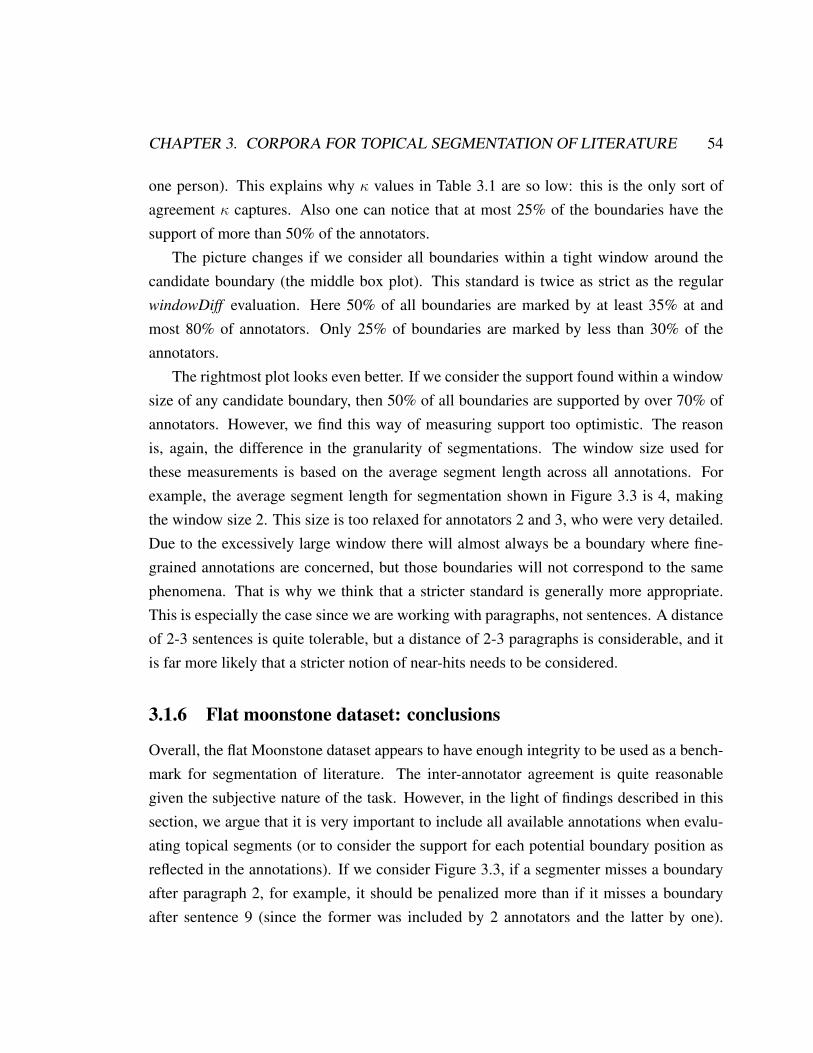
CHAPTER 3. CORPORA FOR TOPICAL SEGMENTATION OF LITERATURE 54
one person). This explains why κ values in Table 3.1 are so low: this is the only sort ofagreement κ captures. Also one can notice that at most 25% of the boundaries have thesupport of more than 50% of the annotators.
The picture changes if we consider all boundaries within a tight window around thecandidate boundary (the middle box plot). This standard is twice as strict as the regularwindowDiff evaluation. Here 50% of all boundaries are marked by at least 35% at andmost 80% of annotators. Only 25% of boundaries are marked by less than 30% of theannotators.
The rightmost plot looks even better. If we consider the support found within a windowsize of any candidate boundary, then 50% of all boundaries are supported by over 70% ofannotators. However, we find this way of measuring support too optimistic. The reasonis, again, the difference in the granularity of segmentations. The window size used forthese measurements is based on the average segment length across all annotations. Forexample, the average segment length for segmentation shown in Figure 3.3 is 4, makingthe window size 2. This size is too relaxed for annotators 2 and 3, who were very detailed.Due to the excessively large window there will almost always be a boundary where fine-grained annotations are concerned, but those boundaries will not correspond to the samephenomena. That is why we think that a stricter standard is generally more appropriate.This is especially the case since we are working with paragraphs, not sentences. A distanceof 2-3 sentences is quite tolerable, but a distance of 2-3 paragraphs is considerable, and itis far more likely that a stricter notion of near-hits needs to be considered.
3.1.6 Flat moonstone dataset: conclusions
Overall, the flat Moonstone dataset appears to have enough integrity to be used as a bench-mark for segmentation of literature. The inter-annotator agreement is quite reasonablegiven the subjective nature of the task. However, in the light of findings described in thissection, we argue that it is very important to include all available annotations when evalu-ating topical segments (or to consider the support for each potential boundary position asreflected in the annotations). If we consider Figure 3.3, if a segmenter misses a boundaryafter paragraph 2, for example, it should be penalized more than if it misses a boundaryafter sentence 9 (since the former was included by 2 annotators and the latter by one).

CHAPTER 3. CORPORA FOR TOPICAL SEGMENTATION OF LITERATURE 55
Conversely, if an automatic segmenter includes a boundary after paragraph 6, it should bepenalized more than if it includes a boundary after paragraph 9 (the former boundary wasnot included by any of the 4 annotators, while the later was included by one person, mak-ing it a more feasible hypothesis). In-depth research on evaluating topical segmenters isbeyond the scope of this research project. However, in [Kazantseva and Szpakowicz, 2012]we propose a simple modification to windowDiff that improves the reliability of evaluationby considering all available annotations. Alternatively, the S metric of Fournier and Inkpen[2012] can be configured to give weights to the boundary positions according to the supportfrom the human annotators.
3.2 The Moonstone dataset 2: a dataset for hierarchicalsegmentation
3.2.1 Overview of the hierarchical dataset
One of the research questions addressed in this dissertation is hierarchical segmentation ofliterature – the task of building a topic-based tree for each chapter/work. Consequently, itis necessary to evaluate the performance of our hierarchical segmenter by comparing itsperformance with segmentations produced by people. This subsection describes a datasetthat we have created for this purpose.
We have already mentioned in the previous section that literature is a genre with uniquecharacteristics and for that reason it is unrealistic to expect that the performance of auto-matic segmenters tested on other datasets would generalize to literary data. This is whywe decided to create our own dataset. Our objectives when creating this dataset were asfollows. Firstly, we wanted to study how people performed when asked to identify hier-archical topical structure in literary data. We wanted to study whether it was a reasonabletask, whether it was difficult or easy for them and whether they agreed between themselves.Secondly, given the general scarcity of datasets for evaluating hierarchical segmenters, wewanted to build a benchmark dataset and make it available to other researchers.
In order to study how people perform hierarchical segmentation of literature, we choseuse a subset of the data used in the flat segmentation study – 9 chapters from the novel The

CHAPTER 3. CORPORA FOR TOPICAL SEGMENTATION OF LITERATURE 56
Moonstone.5 This way, we eventually obtain a dataset that can be used for studying flator hierarchical segmentations, parallels and differences between them or for studying howsegmentations can be applied to higher-level tasks, such as automatic summarization.
In a nutshell, the results of this experiment are slightly less conclusive than those of theprevious one. Firstly, the annotators have found the task considerably more difficult thanthe previous one – this is reflected both in the average time taken to complete the experi-ment and also in the annotators’ notes. The inter-annotator agreement is lower than in theflat dataset but still quite reliable. Interestingly, it seems that the most common type ofdisagreement between the annotators is not so much whether there is a topic shift or not ata given position, but at what level it occurs. In a certain way, this echoes the findings fromthe previous experiment about the fact that people segment at different levels of granular-ity. This may suggest that ultimately hierarchical segmentation is a more appropriate wayof modelling topic structure. However, it also becomes clear that comparing hierarchicalsegmentations and evaluating hierarchical segmenters is considerably more challenging.
The next subsesction (3.2.2) describes in detail how the corpus was constructed. Sub-section 3.2.3 provides the analysis of the data and discusses the inter-annotator agreement.Section 3.2.4 concludes with high-level interpretation and discussion.
3.2.2 Hierarchical moonstone dataset: corpus overview
We chose nine previously annotated chapters of The Moonstone to be used in the hierar-chical segmentation experiment (Chapters 1-2 and 4-10). The choice of the chapters wasmore restricted than in the previous study. Hierarchical segmentation is considerably moretime-consuming than single-level segmentation, therefore there was a very real upper limiton the ultimate length of the chapter.
Objectives. The main objective of this study was studying how people segment lit-erature hierarchically. We wanted to examine the difficulty of the task, inter-annotatoragreement and disagreement patterns between the annotators.
Subjects. The subjects participating in the experiment were undergraduate students ofthe English Department at the University of Ottawa. They were recruited by e-mail andeach received 50 dollars compensation for their participation. We aimed to hire 30 students
5All nine chapters had already been annotated in the previous study.

CHAPTER 3. CORPORA FOR TOPICAL SEGMENTATION OF LITERATURE 57
Figure 3.5: An example of hierarchical segmentation for Chapter 2. (Produced byAnnotator 1).
1. Paragraph 1: My Lady and the diamond
2. Paragraphs 2-5 : Gabriel Betteredges service
(a) Paragraph 2: The Herncastles
(b) Paragraph 3-4: The relationship between Gabriel and his Lady Miss Julia
i. Paragraph 3: The page boyii. Paragraph 4: Moving up in positions
(c) Paragraph 5. Bailiff
3. Paragraphs 6-11: Selina and Gabriel
(a) Paragraph 6: Picking a wife
(b) Paragraphs 7-8: Transition paragraphs
(c) Paragraphs 9-11: Gabriel and Selina, husband and wife
i. Paragraph 9: Thoughts of breaking off the engagementii. Paragraph 10: After the wedding
iii. Paragraph 11. Five years of marriage and two deaths
4. Paragraphs 12-14: Life goes on
(a) Paragraphs 12-13: The wool waist coat
i. Paragraph 12: Fifty years of service to his Ladyii. Paragraph 13: Getting old
(b) Paragraph 14: Accepting age and the less demanding job as house steward
5. Paragraph 15: Penelope making sure Gabriel stays on track and tells the story of thediamond

CHAPTER 3. CORPORA FOR TOPICAL SEGMENTATION OF LITERATURE 58
but eventually we received only 23 annotations. The cohort contained several participantsfrom the first experiment, but mostly the students were new.
Procedure. The students were divided into five groups and each group had to annotatetwo chapters. Group 5 was an exception: since the chapter assigned to them was very long,they annotated a single chapter (in two steps with a check-point in the middle).
The experiment was conducted by e-mail. Initially each group had received detailedinstructions and an example annotation as well as the first chapter to work on. They wererequired to submit their annotation within a week. In the second round of the experiment,the students have received the second chapter to work on. Again, they had a week tocomplete the task.
The instructions asked that the annotator read the chapter and split it into top-levelsegments – according to where there is a perceptible shift of topic. Similarly to the previousexperiment, the annotator had to provide a one-sentence description of what the segment isabout. The annotators had to work with paragraphs as the individual units.
Then the task took on a recursive nature: the annotators had to examine each of thetop-level segments and split them into sub-segments, providing a brief description of each.The annotators were asked to repeat this procedure recursively until they reached the levelof individual paragraphs. However, we allowed them to stop at a higher level if they foundit excessively difficult, asking them to record the difficulties.
Effectively, the annotators were building a detailed hierarchical outline for each chapter.An example annotation is shown in Figure 3.5. This outline was created by an annotatorfor Chapter 2 of The Moonstone (see Appendix A for full text).
Metrics: Analyzing and evaluating the quality of the dataset for hierarchical segmen-tation is considerably more complicated than for flat segmentation. When comparing twosingle-level segmentations, one needs to take into account extra/missing boundaries andalso near hits and misses. If more than two annotations are available, one needs to accountfor the whole pool. However, when the annotation is hierarchical, in addition to all of theabove, one also needs to consider multiple layers of the tree. In the end, when estimatingthe reliability of a pool of hierarchical segmentations, we need to take into account simi-larities and differences (including near misses) within and across layers and also across allavailable annotations.
Traditionally, hierarchical segmenters have been evaluated either by computing win-

CHAPTER 3. CORPORA FOR TOPICAL SEGMENTATION OF LITERATURE 59
Figure 3.6: Example segmentation for Chapter 2. Annotator 2.
1. Paragraphs 1-4: the single life of the narrator (a note: paragraph one sets the time thestory begins)
(a) paragraph 1: the diamonds location
(b) paragraphs 2-4: how he came to be in his career
i. paragraph 2: how he met the ladyii. paragraph 3: how he became hired by the lady
iii. how he came to be promoted to bailiff
2. paragraphs 5-10: life with a love interest before and after marriage
(a) paragraphs 5-8: motivations for finding a wife
i. paragraph 5: lonelinessii. paragraph 6: economics and love
iii. paragraphs 7-8: the lady’s approvalA. paragraph 7: asking for approvalB. paragraph 8: receiving approval
(b) paragraphs 9-10: experiences of marrying and being married to a woman
i. paragraph 9: apprehensions about marriageii. paragraph 10: mediocrity in married life
3. paragraphs 11-15: life as a widower and into old age
(a) paragraph 11: death of the narrator’s wife and first mention of daughter Penelope
(b) paragraphs 12-14: convincing the narrator to alter his occupation
i. paragraph 12: Lady lulls him into security with kindnessii. paragraph 13: narrator realises her plan, and his pride fights against it
iii. paragraph 14: narrator is convinced after reading Crusoe he will feel betterabout it tomorrow
(c) paragraph 15: the difficulty of writing a story without accidentally writing aboutoneself (a note: only technically in his old age, not really about his old age)

CHAPTER 3. CORPORA FOR TOPICAL SEGMENTATION OF LITERATURE 60
dowDiff or Pk per level (e.g., [Eisenstein, 2009]) or by flattening the tree (e.g., [Song et al.,2011]). However, both methods have weaknesses. When reporting the results per level,we do not take into account situations when the segmenter failed to specify a boundary atthe correct level, but perhaps identified it in an adjacent level. When flattening the tree weeffectively lose all information about hierarchical structure and treat the errors at the toplevel equally with the errors at the fine-grained levels.
Carroll [2010] proposes a measure for evaluating hierarchical segmenters. The measureis a version of Pk proposed by Beeferman et al. [1999], adjusted so as to spread the errorover all levels in the segmentation tree. It is designed to give higher weight to the top levelsof the tree and lower weight to the levels towards the bottom:
Epk =1
|R|∑i
ciPk(Ri, Hi) (3.7)
Here R is the set of reference boundaries and H is the set of hypothetical ones, orderedby their prominence (the level in the tree), ci is the weighing factor. The following equationmust also hold:
Ri = {bj : bj ∈ R ∧ j ≤ i} (3.8)
The measure is an improvement over simply applying windowDiff or Pk at each level,but it has a number of shortcomings. For one thing, it inherits all the problems alreadyfound in Pk (listed in Section 3.1.4 and also in [Pevzner and Hearst, 2002]). Additionally,it does not take into account similarities across different levels in the segmentation tree,effectively evaluating each level in isolation.
In Section 3.1.4 we briefly listed some of the problems with the window-based metrics(e.g., windowDiff and Pk). All those issues are just as relevant in hierarchical segmentationas in flat one. For this reason we decided not to use it for analysis. Instead, we decided touse the S metric as our main analytical tool. To be comparable to previous research we alsoreport windowDiff. Section 3.2.3 shows the results, but also illustrates why windowDiff isnot an appropriate metric for hierarchical segmentation analysis.
Recall that the S metric can be interpreted as follows: if we were to change a bound-ary sting bsa into a boundary string bsb, what proportion of the boundaries would remainunchanged? In their paper, Fournier and Inkpen [2012] explain in detail how to use the

CHAPTER 3. CORPORA FOR TOPICAL SEGMENTATION OF LITERATURE 61
(a) Chapter 2, annotator 1
(b) Chapter 2, annotator 2
Figure 3.7: Example hierarchical segmentations for Chapter 2.
metic for single-level segmentation. However, they mention that in fact the metric operatesnot on strings of boundaries, but on strings of sets of boundaries – making it applicable insituation where multiple boundary types are involved, for example in dialogue-act schemasor in hierarchical segmentation.
Figure 3.7 shows two example segmentations for Chapter 2 of The Moonstone (full textis available in Appendix A). The textual outlines created by the annotators are shown inFigures 3.5 and 3.6. While the trees are somewhat similar (and especially if we considerthe textual outlines), it is difficult to say whether they are in fact similar enough. Worse yet,it is not clear which trees are more similar than the others (since of course we have morethan two trees for each chapter).

CHAPTER 3. CORPORA FOR TOPICAL SEGMENTATION OF LITERATURE 62
We can notice that often the annotators disagree on the exact placement of the boundary(especially for transition paragraphs) and on where exactly they should be attached. Bothannotators indicated a shift of topic after Paragraph 1, but annotator 1 separated it into a top-level segment, while annotator 2 attached it to a second-level segment. (The situation is thesame with Paragraph 15. From the annotators’ notes and from reading the text in AppendixA, we can see that these are introductory and concluding paragraphs. Additionally, theyrepresent entry and exit points of an embedded narrative, adding to the complexity of thetask for the annotators).
Comparing two segmentation trees is not intuitive. However, we need to remember thateffectively the branchings in the tree correspond to fluctuations in topic – with branchingsnear the top of the tree indicating relatively significant fluctuations, while branchings nearthe leaves correspond to less pronounced fluctuations or minor digressions. Keeping this inmind, we may flatten the tree representation. Figures 3.8a and 3.8b show the correspondingflattened representations.
Figure 3.8a shows a flattened representation for the tree shown in Figure 3.7a (and,correspondingly, the representation of the tree from Figure 3.7b is given in Figure 3.8b).In this representation, the vertical lines indicate the presence of a boundary. The lengthof the vertical lines represents the level at which the boundary was found in the tree – thelonger the line, the closer to the root the boundary was (and hence the more pronouncedthe fluctuation was). The sets of numbers under each line indicate the levels specifically.The S metric operates on sets of boundary strings – such as appear in the bottom row. Thisis how we will compare topical segmentation trees.

CHAPTER 3. CORPORA FOR TOPICAL SEGMENTATION OF LITERATURE 63
Figure 3.8: Flattened representations of topical trees.
(a) Flattened representation of the tree from Figure 3.7a
2 1 3 15 14 13 12 11 4 5 9 7 6 8 10 paragraph
level 3 (bottom)
level 2
level 1
level 0 (root)
{1} {2} {3} {3,2} {1,2} {2} {} {2} {} {2} {1,2} {3} {2,3} {1,2} {1} levels in the segmentation tree
(b) Flattened representation of the tree from Figure 3.7b
2 1 3 15 14 13 12 11 4 5 9 7 6 8 10 paragraph
level 3 (bottom)
level 2
level 1
level 0 (root)
{2} {3} {3} {1,2,3} {3} {3} {} {2,3} {3} {1,2,3} {2} {3} {3} {2,3} {1,2} levels in the segmentation tree

CHAPTER 3. CORPORA FOR TOPICAL SEGMENTATION OF LITERATURE 64
3.2.3 Hierarchical dataset: corpus analysis
Overall, we have collected 23 annotations for the 9 chapters of The Moonstone. Table3.2 shows what groups of annotators worked on what chapters and the number of peopleper group. Since different groups worked on different chapters, most statistics have beencomputed per group. Whenever overall averages are given for the whole corpus, they aremacro-averages across all groups, unless otherwise indicated.
On average, the annotators took 3.5 hours to complete the task (std.dev. = 1.6). Av-erage depth of the tree is 3.00 levels (std.dev. = 0.65), suggesting that the annotatorsprefer shallow but broad structures. Table 3.3 reports average breadth of the tree at differ-ent levels. The breadth at Level 4 is lower than that at level 3, indicating that only a smallpercentage of the entire tree was annotated at a level deeper than 3. We hypothesize thatthese shallow broad structures are due to the fact that it is difficult for people to create deeprecursive structures in their mental representations. However, we do not have any hard datato support this hypothesis.
Many of the annotators specifically commented on the difficulty of the task. Nine outof 23 people included comments ranging from notes about specific places to general com-ments about their lack of confidence. 4 annotators found several (specific) passages theyhad trouble with.
One simple way to estimate the quality of the annotations is by computing pair-wisewindowDiff at each level. Figure 3.9 shows the averages of pairwise windowDiff valuesacross all annotations.6 The values seem to be lowest for the top level (Level 1), indicatingthe best agreement near the root of the tree. Overall, they rise gradually as we go deeperinto the tree, corresponding to worse agreement. However, these values should be takenwith caution. In addition to all the shortcomings listed in Section 3.1.4, these values arecomputed for the whole sequence at each level. This rarely makes much sense except for thetop level since the trees are not balanced and not the whole sequence has been segmented atdeeper levels (for example in Figure 3.7a only four nodes appear at the bottom level). Dueto these concerns, we use the S metric as the primary tool for analyzing the hierarchicaldataset.
Figure 3.10 reports average pairwise S similarity across all annotators. The values here
6windowDiff values are reported per annotator here. For each annotator we computed windowDiff valuesagainst all other annotators in their group. Figure 3.9 reports averages of these values.

CHAPTER 3. CORPORA FOR TOPICAL SEGMENTATION OF LITERATURE 65
Table 3.2: Chapter assignments per groups of annotators.
Group Chapters Number ofannotators
Group1 ch1, ch4 6Group 2 ch2, ch6 5Group 3 ch5, ch7 6Group 4 ch8, ch9 4Group 5 ch10 3
are computed pairwise for each possible pair of annotators and then the mean is reportedfor each annotator. We are not aware of another dataset for hierarchical segmentation withmore than one annotator, hence it is somewhat difficult to put these numbers in context.However, we know that S ranges from 0 for absolutely dissimilar segmentations to 1 foridentical ones. Therefore, the numbers in Figure 3.10 seem to indicate a reasonable levelof inter-annotator similarity.
Fournier and Inkpen [2012] also propose versions of the widely used inter-annotatoragreement coefficients κ and π that are suitable for text segmentation (i.e., they take intoaccount near hits and near misses). Figure 3.11 shows the values of S-based variants ofκ and π (and also, for completeness, the values of pairwise S) per chapter. While thereis no other hierarchical dataset for which these values have been computed, it is generallythought that agreement above 0.7 is acceptable (see the scale in Landis and Koch [1977]).
Recall that the value of S can be interpreted as 1 - e, normalized by the length of thestring, where e is the number of edit operations necessary to turn one boundary string intoanother. In the hierarchical version of the software, three edit operations are possible: ad-
Table 3.3: Average breadth of the trees at different levels.
Level Meanbreadth
Std. dev.
Level 1 6.53 3.41Level 2 17.55 7.03Level 3 17.63 10.61Level 4 8.8 9.39

CHAPTER 3. CORPORA FOR TOPICAL SEGMENTATION OF LITERATURE 66
Figure 3.9: windowDiff values across levels of hierarchical segmentations.
ditions/deletions, transpositions and substitutions.7 Additions/deletions and transpositionsare intra-level edit operations, while substitutions are inter-level operations. Figure 3.12breaks down the sum total of necessary edit operations involved in computing S. For clar-ity, these values are normalized by chapter lengths multiplied by the number of annotationsper chapter.
From Figure 3.12 it is easy to see that transposition errors are relatively rare, mean-ing that in our case near hits and misses do not play a critical role. On the other hand,missing/extra boundaries (shown under the legend additions) are common. Equally, if notmore, common are substitution errors – situations where the annotators disagreed not onwhether or not there is a topic change, but on how prominent it is (i.e., at what level inthe segmentation tree it occurs). This is an important finding. It shows that, while overallagreement in hierarchical segmentation tasks is lower, a significant portion of it is aboutthe level, not about the presence of absence of topical shifts.
7Additions/deletions correspond to the cases where a boundary needs to be added or removed within thesame level. Transpositions correspond to near hits/near misses – where the boundaries boundary positions donot align but are near, within a specified transposition window within the same level. Substitutions correspondto situations where the levels at which the boundaries are placed differ. For example in Figures 3.7a and 3.7bAnnotator 1 placed a boundary after paragraph 1 at level 1, which Annotator 2 placed at level 2.

CHAPTER 3. CORPORA FOR TOPICAL SEGMENTATION OF LITERATURE 67
Figure 3.10: Mean pairwise S values for all annotators.
●
●●
●
●
●
●
●
●
●
●
●
●●
●
●
●
● ●
●
●
●
●
●
5 10 15 20
0.72
0.74
0.76
0.78
0.80
0.82
0.84
0.86
Pairwise S per coder and mean S value
Coder id
S va
lue

CHAPTER 3. CORPORA FOR TOPICAL SEGMENTATION OF LITERATURE 68
Figure 3.11: S-based inter-annotator agreement per chapter.
3.2.4 Conclusions about the hierarchical dataset
We have created a dataset for hierarchical segmentation of literary data. Hierarchical seg-mentation is more difficult than flat segmentation – both cognitively (for people) and com-putationally (for systems). Yet, our dataset appears to have enough integrity to serve as abenchmark. As expected, there is a fair amount of disagreement between the annotators.However, considering the nature of the task, there is also substantial agreement.
The analysis also revealed that substantial portion of disagreement is disagreementabout the magnitude of topic fluctuations, not about whether there is a topic change ornot. We do not have the results to support this hypothesis, but it is possible that our require-ment to summarize each segment added to this type of disagreement. It is likely that whencreating this outline people are more constrained, probably invoking schemas from similardocuments that they have previously read, thus influencing the points of attachments in thetree.
However, the dataset appears suitable for our purposes of evaluating automatic hierar-chical segmenters.

CHAPTER 3. CORPORA FOR TOPICAL SEGMENTATION OF LITERATURE 69
Figure 3.12: Edit operations when computing S. Number of edits / chapter length * numberof annotations
ch1 ch10 ch2 ch4 ch5 ch6 ch7 ch8 ch9
additionsinter−level substitutionstranspositions
Errors per chapter (normalized)
Chapter id
Nor
mal
ized
num
ber
of e
rror
s
0.0
0.5
1.0
1.5

CHAPTER 3. CORPORA FOR TOPICAL SEGMENTATION OF LITERATURE 70
3.3 Conclusions
In this chapter we have described two datasets of topical segmentations of literature thatwere created in the course of this work. The datasets can be used to evaluate topical seg-menters as well as to study how people perform this task.
The results of our analysis suggest that the Moonstone corpora have enough integrityto be used as benchmark datasets. The inter-annotator agreement is higher on the flatMoonstone dataset. The agreement on the hierarchical dataset is more difficult to measureand to interpret. Creating trees as opposed to sequences of segments is more difficult forboth people and automatic segmenters and the drop in agreement is reasonable.
Both datasets are freely available for public use and study. One of the research avenuesthat we have left unexplored in this work is the study of the manually written outlinescreated by the annotators. It would be very interesting to compare them qualitatively andto explore if disagreements about the granularity of segmentation and about the levels ofparticular boundaries can be explained by the annotators’ interpretations of the documentas captured in the outlines. However, we leave this fascinating project for future work.

Chapter 4
Affinity Propagation for textsegmentation
In the previous chapter, we have described two studies of how people segment fiction ac-cording to topical fluctuations. Ultimately, it is our objective to create trees similar tothose in Figures 3.7a and 3.7b automatically. This chapter describes an algorithm for textsegmentation proposed in this work. This document describes an implemented and prelim-inarily evaluated algorithm for flat text segmentation. (In the next chapter we will extendthe segmenter to build tree-like structures). While we are primarily interested in segment-ing literary texts, we will also report the results on two other benchmark datasets – oneconsisting of transcribed speech and one consisting of chapters from medical textbooks.We do this to see how the performance of our segmenter generalizes to other challengingdata types and also to allow fair comparison with the other segmenters which were built,fine-tuned and tested by their authors on those datasets. The segmenter described in thischapter is suitable for any type of data and is not literature-specific.
In this work, we use exemplar-based clustering to model the topical structure of the text.Each cluster has a central point – an exemplar – that somehow ‘summarizes’ the unifyingquality of the cluster. The points are assigned to clusters based on their similarity to theexemplars. When computing cluster assignments, the program attempts to maximize thequantity known as net similarity – the total sum of similarities between all points and theirrespective exemplars.
If we extrapolate this abstract problem definition into the domain of text segmentation,
71

CHAPTER 4. AFFINITY PROPAGATION FOR TEXT SEGMENTATION 72
then ultimately we have the following. Using exemplar-based clustering, we will attemptto identify spans of text that have certain degree of topical unity to them. The clustersmust necessarily consist of adjacent units, so as to qualify as segments. Each such seg-ment/cluster is characterized by a central unit – exemplar– which best captures what itis about. The clusters are computed so as to maximize the total sum of similarities be-tween each unit and its exemplar. The units used will be discussed in detail in Section 4.3which describes the experimental setting. However, for our main datasets (the Moonstone
datasets) we will use paragraphs as units.The problem of exemplar-based clustering is NP-complete and has been extensively
studied (e.g., [Mahajan et al., 2009]). Some of the classical solutions are the k-means/k-medoid algorithms [Bishop, 2006] and the Expectation Maximization (EM) algorithms[Mclachlan and Krishnan, 1996]. There are two main problems with these approaches.Firstly, they are known to be highly sensitive to well-selected initialization points. Sec-ondly, on each iteration they take into account only a part of the available information,which makes them prone to finding local as opposed to global maxima. Recently, Freyand Dueck [2007], Givoni and Frey [2009] proposed a new clustering algorithm, AffinityPropagation (AP) that dramatically improved both the speed of clustering and the qualityof solutions. This is the algorithm that we have chosen to address our text segmentationproblem.
Affinity Propagation operates by iteratively passing messages between all available datapoints (in our case, given that we work with text, it would correspond to all paragraphs orall sentences in a document). It takes as inputs a matrix of similarities between all pointsand on each iteration considers them all as potential exemplars. This global view of thedata and of the possible assignments often leads to better-quality assignments than otheralgorithms. Technically, it is an instance of so-called loopy-belief propagation on a factorgraph with cycles. Such algorithms are not guaranteed to find a globally optimal solution.They are not even guaranteed to converge. However, in practice, they have been used toachieve state-of-the-art performance in error-correcting decoding, image processing anddata compression, to name a few.
In practice and in our setting, AP will operate in the following manner. On each iterationall nodes (corresponding to paragraphs to be clustered) send two types of messages: anavailability message and a responsibility message. A responsibility message reflects how

CHAPTER 4. AFFINITY PROPAGATION FOR TEXT SEGMENTATION 73
likely the receiver is to be an exemplar for the sender given all other potential exemplars(all other paragraphs). An availability message reflects how likely the sender is to be anexemplar for the receiver given the evidence from all other paragraphs it exemplifies. Themessages are sent iteratively until a solution emerges or until the program runs out of time.
This chapter presents a version for flat segmentation. The system is called Affinity
Propagation for Segmentation – APS. The results are encouraging: APS performs on paror slightly better than two state-of-the art topical segmenters. The hierarchical version(HAPS) is described in the following chapter.
The flat version of APS operates by iteratively passing messages in a factor graph[Kschischang et al., 2001] until a good set of segments emerges. Each iteration considersall similarities – takes into account all available information. An iteration includes sendingat most O(N2) messages. For the majority of realistic segmentation tasks, however, theupper bound is O(MN) messages, where M is a constant. This is more computationallyexpensive than the requirements of locally informed segmentation algorithms such as thosebased on HMM or CRF (see Section 2.4), but for a globally-informed algorithm the re-quirements are very reasonable. APS works on an already pre-compiled similaritiy matrix,so it offers flexibility in the choice of similarity metrics.
In addition to requiring a similarity matrix, the algorithm also takes as input a vectorof preference values. Preferences reflect a priori beliefs of how likely each paragraph isto be an exemplar. For example, if clustering news articles, one may want to give higherpreference values to the leading sentences in each paragraph to reflect the fact that theleading sentence often summarizes the paragraph in that genre.
The desired granularity of segmentation can be set by adjusting preferences. This is adesired and often overlooked quality – in a realistic situation the number of segments isalmost always unknown. Additionally, since each cluster/segment has an exemplar, we donot only get the information about where the topic changes, but also a rough gist of whateach segment is about.
This chapter is structured as follows. Section 4.1 offers some background of message-passing algorithms in factor graphs and on the original Affinity Propagation. Section 4.2describes the derivation of APS. Section 4.3 contains experimental results and Section 4.4closes the chapter with conclusions and a discussion.
Parts of this chapter are rather technical. We tried to keep such sections self-contained.

CHAPTER 4. AFFINITY PROPAGATION FOR TEXT SEGMENTATION 74
The readers not interested in mathematics and in the derivation of the algorithm will notmiss much if they skip Sections 4.1 and 4.2.
4.1 Background: factor graphs and affinity propagationfor clustering
4.1.1 Factor graphs and the max-sum algorithm
This section provides a brief but hopefully self-sufficient overview of factor-graphs as aframework and also of the original Affinity Propagation (for clustering) algorithm.
The APS algorithm is an instance of belief propagation on a cyclic factor graph. Inorder to explain the derivation of the algorithm, we will first briefly introduce factor graphsas a framework.
Many computational problems can be reduced to maximizing the value of a multi-variate function F (x1, . . . , xn) which can be approximated by a sum of simpler functions.In Equation 4.1, H is a set of discrete indices and fh is a local function with argumentsXh ⊂ {x1, . . . , xn}:
F (x1, . . . , xn) =∑h∈H
fh(Xh) (4.1)
Factor graphs offer a concise graphical representation for such problems. A globalfunction F which can be decomposed into a sum ofM local functions fh can be representedas a bi-partite graph with M function nodes and N variable nodes (M = |H|). Figure 4.1shows an example of a factor graph for F (x1, x2, x3, x4) = f1(x1, x2, x3) + f2(x2, x3, x4).The factor (or function) nodes are dark squares, the variable nodes are light circles.
The well-known max-sum algorithm [Bishop, 2006] seeks a configuration of variableswhich maximizes the objective function. It is guaranteed to find the maximum in acyclicfactor graphs, but in graphs with cycles, neither convergence nor optimality are guaranteed[Pearl, 1982]. Yet, in practice good approximations can be achieved. The max-sum algo-rithm amounts to propagating messages from function nodes to variable nodes and fromvariable nodes to function nodes. A message sent from a variable node x to a function nodef is computed as a sum of the incoming messages from all neighbours of x other than f(the sum is computed for each possible value of x):
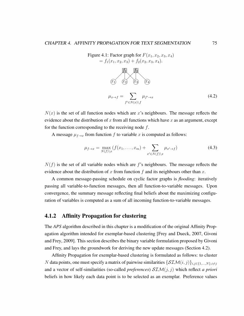
CHAPTER 4. AFFINITY PROPAGATION FOR TEXT SEGMENTATION 75
Figure 4.1: Factor graph for F (x1, x2, x3, x4)= f1(x1, x2, x3) + f2(x2, x3, x4).
f1 f2
x1 x2 x3 x4
µx→f =∑
f ′∈N(x)\f
µf ′→x (4.2)
N(x) is the set of all function nodes which are x’s neighbours. The message reflects theevidence about the distribution of x from all functions which have x as an argument, exceptfor the function corresponding to the receiving node f .
A message µf→x from function f to variable x is computed as follows:
µf→x = maxN(f)\x
(f(x1, . . . , xm) +∑
x′∈N(f)\x
µx′→f ) (4.3)
N(f) is the set of all variable nodes which are f ’s neighbours. The message reflects theevidence about the distribution of x from function f and its neighbours other than x.
A common message-passing schedule on cyclic factor graphs is flooding: iterativelypassing all variable-to-function messages, then all function-to-variable messages. Uponconvergence, the summary message reflecting final beliefs about the maximizing configu-ration of variables is computed as a sum of all incoming function-to-variable messages.
4.1.2 Affinity Propagation for clustering
The APS algorithm described in this chapter is a modification of the original Affinity Prop-agation algorithm intended for exemplar-based clustering [Frey and Dueck, 2007, Givoniand Frey, 2009]. This section describes the binary variable formulation proposed by Givoniand Frey, and lays the groundwork for deriving the new update messages (Section 4.2).
Affinity Propagation for exemplar-based clustering is formulated as follows: to clusterN data points, one must specify a matrix of pairwise similarities {SIM(i, j)}i,j∈{1,...,N},i 6=jand a vector of self-similarities (so-called preferences) SIM(j, j) which reflect a priori
beliefs in how likely each data point is to be selected as an exemplar. Preference values

CHAPTER 4. AFFINITY PROPAGATION FOR TEXT SEGMENTATION 76
Figure 4.2: Factor graph for affinity propagation.
E1 Ej EN
I1
Ii
IN
c11 c1j c1N
ci1 cij ciN
cN1 cNj cNN
S11 S1j S1N
Si1 Sij SiN
SN1 SNj SNN
occupy the diagonal of the similarity matrix. The algorithm then assigns each data point toan exemplar so as to maximize net similarity – the sum of similarities between all pointsand their respective exemplars; this is expressed by Equation 4.7. Figure 4.2 shows aschematic factor graph for this problem, with N2 binary variables. cij = 1 iff point j isan exemplar for point i. Function nodes Ej enforce a coherence constraint: a data pointcannot exemplify another point unless it is an exemplar for itself:
Ej(c1j, . . . , cNj) =
−∞ if cjj = 0 ∧ cij = 1
for some i 6= j
0 otherwise
(4.4)
An I node encodes a single-cluster constraint: each data point must belong to exactly oneexemplar – and therefore to one cluster:
Ii(ci1, . . . , ciN) =
−∞ if∑
j cij 6= 1
0 otherwise(4.5)
An S node encodes user-defined similarities between data points and candidate exemplars

CHAPTER 4. AFFINITY PROPAGATION FOR TEXT SEGMENTATION 77
(SIM(i, j) is the similarity between points i and j):
Sij(cij) =
SIM(i, j) if cij = 1
0 otherwise(4.6)
Equation 4.7 shows the objective function which we want to maximize: a sum of similari-ties between data points and their exemplars, subject to the two constraints (coherence andsingle-cluster per point).
S(c11, . . . , cNN) =∑i,j
Si,j(cij) +∑i
Ii(ci1, . . . , ciN) (4.7)
+∑j
Ej(c1j, . . . , cNj)
According to Equation 4.3, the computation of a single factor-to-variable message involvesmaximizing over 2n configurations. E and I , however, are binary constraints and evalu-ate to −∞ for most configurations. This drastically reduces the number of configurationswhich can maximize the message values. Given this simple fact, Givoni and Frey [2009]show how to reduce the necessary update messages to only two types of scalar ones: avail-
abilities (α) and responsibilities (ρ).1
A responsibility message ρij , sent from a variable node cij to function node Ej , reflectsthe evidence of how likely j is to be an exemplar for i given all other potential exemplars:
ρij = SIM(i, j)−maxk 6=j
(SIM(i, k) + αik) (4.8)
An availability message αij , sent from a function node Ej to a variable node cij , reflects
1Normally, each iteration of the algorithm sends five types of two-valued messages: to and from functionsE and I and a message from functions S. Fortunately, the messages sent to and from E factors to the variablenodes subsume the three other message types and it is not necessary to compute them explicitly. See [Givoniand Frey, 2009, p.195] for details.

CHAPTER 4. AFFINITY PROPAGATION FOR TEXT SEGMENTATION 78
how likely point j is to be an exemplar for i given the evidence from all other data points:
αij =
∑k 6=j
max[ρkj, 0] if i = j
min[0, ρjj +∑k/∈{i,j}
max[ρkj, 0]] if i 6= j(4.9)
Let γij(l) be the message value corresponding to setting variable cij to l, l ∈ {0, 1}. Insteadof sending two-valued messages (corresponding to the two possible values of the binaryvariables), we can send the difference for the two possible configurations: γij = γij(1) −γij(0) – effectively, a log-likelihood ratio.
The algorithm converges when the set of points labelled as exemplars remains un-changed for a pre-determined number of iterations. When the algorithm terminates, mes-sages to each variable are added together. A positive final message indicates that the mostlikely value of a variable cij is 1 (point j is an exemplar for i), a negative message indicatesthat it is 0 (j is not an exemplar for i).
4.2 Affinity Propagation for flat segmentation
Affinity Propagation is a generic algorithm for clustering data points - proteins, locationson the map, images or sentences. In this section we explain how to adapt this genericalgorithm for flat topical segmentation. In this dissertation, we work only with textual data,so we feel that it is more appropriate to refer to exemplars as segment centres. A segment
centre is a sentence or a paragraph that best exemplifies the contents of its segment.2
In this setting, the data points are atomic units of text to be segmented (usually sen-tences or paragraphs. For clarity, we refer to them as sentences throughout this chapter,but paragraphs or arbitrary spans of text are all valid options). There are two inputs intothe segmentation algorithm. Firstly, a matrix of similarities between all data points in thedocument (sentence or paragraphs) which may be sparse. Secondly, a vector or preferences
- values that specify a priori likelihood of how likely each data point is to be chosen as a
2The term centre makes no reference to the position of the sentence with respect to the segment around it.Any sentence in a segment can be its centre, including the opening or the closing sentence. It is a centre onlybecause of its content, not because of its position.

CHAPTER 4. AFFINITY PROPAGATION FOR TEXT SEGMENTATION 79
Figure 4.3: Example of valid configuration of hidden variables {cij} for clustering.
Figure 4.4: Example of valid configuration of hidden variables {cij} for segmentation.
segment centre. There must be one preference value for each data point, the vector may beuniform. The algorithm produces two outputs: segment boundaries and segment centres foreach identified segment. A segment centre is a data point that best describes the contentsof that segment. Given a document, we want to assign each sentence to a segment centreso as to maximize net similarity.
The new formulation relies on the same underlying factor graph (Figure 4.2). A binaryvariable node cij is set to 1 iff sentence j is the segment centre for sentence i. Whenclustering is the objective, a cluster may consist of points coming from anywhere in thedata sequence. When segmentation is the objective, a segment must consist of a solidblock of points around the segment centre. Figures 4.3 and 4.4 show, for a toy problemwith 5 data points, possible valid configurations of variables {cij} for clustering and forsegmentation respectively.
To formalize this new linearity requirement, we elaborate Equation 4.4 into Equa-tion 4.10. Ej evaluates to −∞ in three cases. Case 1 is the original coherence constraint.Case 2 states that no point k may be in the segment with a centre in j, if k lies before thestart of the segment (the sequence c(s−1)j = 0, csj = 1 necessarily corresponds to the startof the segment). Case 3 handles analogously the end of the segment.

CHAPTER 4. AFFINITY PROPAGATION FOR TEXT SEGMENTATION 80
Ej =
−∞ 1. if cjj = 0 ∧ cij = 1 for some i 6= j
2. if cjj = 1 ∧ csj = 1 ∧ c(s−1)j = 0
∧ ckj = 1 for some s ≤ j, k < s− 1
3. if cjj = 1 ∧ cej = 1 ∧ c(e+1)j = 0
∧ ckj = 1 for some e ≥ j, k > e+ 1
0 otherwise
(4.10)
The E function nodes are the only changed part of the factor graph, so we only mustre-derive α messages (availabilities) sent from factors E to variable nodes. A function-to-variable message is computed as shown in Equation 4.11 (elaborated Equation 4.3), andthe only incoming messages to E nodes are responsibilities (ρ messages):
µf→x = maxN(f)\x
(f(x1, . . . , xm) +∑
x′∈N(f)\x
µx′→f ) = (4.11)
maxcij , i 6=j
((Ej(c1j, . . . , cNj) +∑
cij , i 6=j
ρij(cij)))
We need to compute the message values for the two possible settings of binary variables– denoted as αij(1) and αij(0) – and propagate the difference αij = αij(1) – αij(0).
Consider the case of factor Ej sending an α message to the variable node cjj (i.e.,i = j). If cjj = 0 then point j is not its own segment centre and the only valid configurationis to set all other cij to 0:
αjj(0) = maxcij ,i 6=j
(Ej(c1j, . . . , cNj) +∑cij ,i 6=j
ρij(cij)) (4.12)
=∑i 6=j
ρij(0)
To compute αij(1) (point j is its own segment centre), we only must maximize over config-urations which will not correspond to cases 2 and 3 in Equation 4.10 (other assignments aretrivially non-optimal because they would evaluate Ej to −∞). Let the start of a segmentbe s, 1 ≤ s ≤ j and the end of the segment be e, j ≤ e ≤ N . We only need to considerconfigurations such that all points between s and e are in the segment while all others are

CHAPTER 4. AFFINITY PROPAGATION FOR TEXT SEGMENTATION 81
not. The following picture shows a valid configuration.3
1 s j e N
To compute the message αij(1), i = j, we have:
αjj(1) =j
maxs=1
[s−1∑k=1
ρkj(0) +
j−1∑k=s
ρkj(1)]+ (4.13)
Nmaxe=j
[e∑
k=j+1
ρkj(1) +N∑
k=e+1
ρkj(0)]
Subtracting Equation 4.12 from Equation 4.13, we get:
αjj = αjj(1)− αjj(0) = (4.14)
jmaxs=1
(
j−1∑k=s
ρkj) +N
maxe=j
(e∑
k=j+1
ρkj)
Now, consider the case of factor Ej sending an α message to a variable node cij otherthan segment centre j (i.e., i 6= j). Two subcases are possible: point i may lie before thesegment centre j (i < j), or it may lie after the segment centre (i > j).
The configurations which may maximize αij(1) (the message value for setting the hid-den variable to 1) necessarily conform to two conditions: point j is labelled as a segmentcentre (cjj = 1) and all points lying between i and j are in the segment. This corresponds toEquation 4.15 for i < j and to Equation 4.16 for i > j. Pictorial examples of correspond-ing valid configurations precede the equations.
3Variables cij set to 1 are shown as shaded circles, to 0 – as white circles. Normally, variables form acolumn in the factor graph; we transpose them to save space.

CHAPTER 4. AFFINITY PROPAGATION FOR TEXT SEGMENTATION 82
1 s i j e N
αij, i<j(1) =i
maxs=1
[s−1∑k=1
ρkj(0) +i−1∑k=s
ρkj(1)]+ (4.15)
j∑k=i+1
ρkj(1) +N
maxe=j
[e∑
k=j+1
ρkj(1) +N∑
k=e+1
ρkj(0)]
1 s j i e N
αij, i>j(1) =j
maxs=1
[s−1∑k=1
ρkj(0) +
j−1∑k=s
ρkj(1)]+ (4.16)
i−1∑k=j
ρkj(1) +N
maxe=i
[e∑
k=i+1
ρkj(1) +N∑
k=e+1
ρkj(0)]
To compute the message value for setting the hidden variable cij to 0, we again distin-guish between i < j and i > j and consider whether cjj = 1 or cjj = 0 (point j is / is not asegment centre). For cjj = 0 the only optimal configuration is cij = 0 for all i 6= j. For cjj= 1 the set of possible optimal configurations is determined by the position of point i withrespect to point j. Following the same logic as in the previous cases we get Equation 4.17for i < j and Equation 4.18 for i > j.
1 i s j e N
αij(0) = max(∑k/∈i,j
ρkj(0), (4.17)
i−1∑k=1
ρkj(0) +j
maxs=i+1
[s−1∑k=i+1
ρkj(0) +
j−1∑k=s
ρkj(1)]+
ρjj(1) +N
maxe=j
[e∑
k=j+1
ρkj(1) +N∑
k=e+1
ρkj(0)])

CHAPTER 4. AFFINITY PROPAGATION FOR TEXT SEGMENTATION 83
1 s j e i N
αij(0) = max(∑k/∈i,j
ρkj(0), (4.18)
jmaxs=1
[s−1∑k=1
ρkj(0) +
j−1∑k=s
ρkj(1)]+
ρjj(1) +i−1maxe=j
[e∑
k=j+1
ρkj(1) +i−1∑
k=e+1
ρkj(0)]
N∑k=i+1
ρkj(0))
We omit the details of subtracting Equation 4.17 from 4.15 and Equation 4.18 from 4.16.The final update rules for both i < j and i > j appear in Algorithm 1, where we summarizethe whole process.
The equations look cumbersome, but they are trivial to compute. Every summand cor-responds to finding the most likely start or end of the segment, taking into account fixed
information. When computing messages for any given sender node, we can remember themaximizing values for neighbouring recipient nodes. For example, after computing theavailability message from factor Ej to cij , we must only consider one more responsibilityvalue when computing the message from Ej to variable c(i+1)j . The cost of computing amessage is thus negligible.
When the matrix is fully specified, each iteration requires passing 2N2 messages, sothe algorithm runs in O(N2) time and requires O(N2) memory (to store the similarities,the availabilities and the responsibilities). When performing segmentation, however, theuser generally has some idea about the average or maximum segment length. In such morerealistic cases, the input matrix of similarities is sparse – it is constructed by sliding awindow of size M . M usually needs to be at least twice the maximum segment length orthrice the average segment length. Each iteration, then, involves sending 2MN messagesand the storage requirements are also O(MN).
As is common in loopy belief propagation algorithms, both availability and responsibil-ity messages are dampened to avoid overshooting and oscillating. The dampening factor isλwhere 0.5 ≤ λ < 1. In our experiments we found that the value of λ does not significantly

CHAPTER 4. AFFINITY PROPAGATION FOR TEXT SEGMENTATION 84
influence the results. We used λ = 0.9 in most experiments.
newMsg = λ ∗ oldMsg + (1− λ)newMsg (4.19)
The APS algorithm is unsupervised. It only benefits from a small development set to fine-tune a few parameters: preference values and the dampening factor. APS does not require(nor allow) specifying the number of segments beforehand. The granularity of segmenta-tion is adjusted through preference values; this reflect how likely each sentence is to beselected as a segment centre. (This translates into the cost of adding a segment.)
Because each message only requires the knowledge about one column or row of thematrix, the algorithm can be easily parallelized.
In our experiments, the system runs until convergence or for a maximum of 1000 it-erations. Convergence is defined as a situation where the set of segment centres remainsunchanged for 100 iterations.

CHAPTER 4. AFFINITY PROPAGATION FOR TEXT SEGMENTATION 85
Algorithm 1 Affinity Propagation for Segmentation
1: input: 1) a set of pairwise similarities {SIM(i, j)}(i,j)∈{1,...,N}2 , SIM(i, j) ∈ R; 2)a set of preferences (self-similarities) {SIM(i, i)}i∈{1,...,N} indicating a priori likeli-hood of point i being a segment centre
2: initialization: ∀i, j : αij = 0 (set all availabilities to 0)3: repeat4: iteratively update responsibilities (ρ) and availabilities (α)5:
∀i, j : ρij = SIM(i, j)−maxk 6=j
(SIM(i, k) + αik)
6:
∀i, j : αij =
jmaxs=1
(
j−1∑k=s
ρkj) +N
maxe=j
(e∑
k=j+1
ρkj) if i = j
min[i
maxs=1
i−1∑k=s
ρkj +
j∑k=i+1
ρkj +N
maxe=j
e∑k=j+1
ρkj,
imaxs=1
i−1∑k=s
ρkj +j
mins=i+1
s−1∑k=i+1
ρkj] if i < j
min[j
maxs=1
j−1∑k=s
ρkj +i−1∑k=j
ρkj +N
maxe=i
e∑k=i+1
ρkj,
i−1mine=j
i−1∑k=e+1
ρkj +N
maxe=i
e∑k=i+1
ρkj] if i > j
7: until convergence8: compute the final configuration of variables: ∀i, j j is the centre for i iff ρij + αij > 09: output: segment centre assignments

CHAPTER 4. AFFINITY PROPAGATION FOR TEXT SEGMENTATION 86
4.3 Experimental settings
This section reports empirical evaluation of the flat APS segmenter. The development andimplementation of the hierarchical segmenter are described in the next chapter.
Datasets. We evaluate the performance of the flat APS algorithm on four datasets. Thefirst dataset is the Moonstone dataset for flat segmentation described in Chapter 3. Thesecond dataset consists of 85 novels collected from the Project Gutenberg website.4 Theother two are demanding benchmark datasets for topical segmentation. We decided to useadditional data in order to have a more stereoscopic picture of the performance of oursegmenter.
The Moonstone dataset is described in detail in the previous chapter (recall that itconsists of 20 chapters from The Moonstone segmented by 4-6 people per chapter).
The second dataset consists of 85 works of fiction downloaded from Project Gutenberg.The segment boundaries correspond to chapter breaks or to breaks between individual sto-ries. They were inserted automatically using HTML markup in the downloaded files.
The third dataset was compiled by Malioutov and Barzilay [2006]. It consists of man-ually transcribed and segmented lectures on Artificial Intelligence. This dataset is particu-larly interesting to us because transcribed speech is likely to have low word repetition rate– similarly to literature. This property makes segmentation of both genres challenging andfascinating at the same time.
The last dataset consists of 227 chapters from medical textbooks [Eisenstein and Barzi-lay, 2008]. In this dataset, the gold standard segment boundaries correspond to sectionbreaks specified by the authors. While medical textbooks are not an example of informalwriting, the dataset was included because it is a rather demanding benchmark.
The datasets exhibit different characteristics. The lectures, the novels and the Moon-
stone dataset are challenging because they are less cohesive than the medical textbooks.The textbooks are cognitively more difficult to process and the authors rely on repetitionof terminology to facilitate comprehension. Since lexical repetition is the main source ofinformation for text segmentation, we expect a higher performance on this dataset. Tran-scribed speech, on the other hand, is considerably less cohesive. The lecturer makes aneffort to speak in “plain language” and to be comprehensible, relying less on terminology.
4http://http://www.gutenberg.org/

CHAPTER 4. AFFINITY PROPAGATION FOR TEXT SEGMENTATION 87
The use of pronouns is very common, as is the use of examples.For different reasons, the flat Moonstone dataset is also very challenging. Repeated use
of the same words is not common in fiction, which is a problem, since all three segmentersrely only on lexical information. Additionally, since this is a novel, the text is full of dia-logues and small digressions. Additionally, this part of the novel is an embedded narrativewhich shifts back and forth between the time of narration and the main story line (i.e., thecharacter named Betteredge is telling the story of The Moonstone). All these characteristicsmake the dataset very challenging.
Baselines. We compare the performance of APS with two recent segmenters: the Mini-
mum Cut Segmenter [Malioutov and Barzilay, 2006] and the Bayesian Segmenter [Eisen-stein and Barzilay, 2008]. The authors have made Java implementations publicly available.For the Minimum Cut Segmenter, we select the best parameters using the script includedwith that distribution. The Bayesian segmenter automatically estimates all necessary pa-rameters from the data.
All results are reported using a form of cross validation. The Moonstone and the lecturesdatasets are quite small, so we use 5-fold cross validation. For the clinical dataset and thefiction one we use ten-fold cross validation. On each iteration, the best parameters arechosen automatically using 3 development files, while the rest of the files in the fold areused for testing. The folds are created so that in the end of the experiment all available fileshave been used for testing, but at most 3 × n randomly chosen files are used for training(since there is no need for more data to set the parameters).
Preprocessing and the choice of similarity metric. As described in Section 4.2, theAPS algorithm takes as inputs a matrix of pairwise similarities between sentences in thedocument and also, for each sentence, a preference value.
We estimated topical similarity between sentences using two methods: cosine simi-larity using a simple bag-of-words representation and also the model of textual similaritydescribed in [Bar et al., 2012]. This model corresponds to roughly the best system in theSemEval 2012 Textual Similarity competition.5 The model is available as a part of theDKPro Similarity framework [Bar et al., 2013]. Further in this work we refer to thissimilarity measure as STS-2012 baseline (because it is used as the baseline for the nextSemEval Textual Similarity track).
5The system described in [Bar et al., 2012] scored best in two out of three evaluations.

CHAPTER 4. AFFINITY PROPAGATION FOR TEXT SEGMENTATION 88
The STS-2012 baseline consists of a log linear regression model trained on the SemEval2012 training data. It combines an assortment of measures of textual similarity to comeup with its judgements. The metrics include n-gram overlap, word similarity measuresbased on ontologies, word similarity estimated using Distributional Thesaurus [Lin, 1998],Explicit Semantic Analysis [Gabrilovich and Markovitch, 2007] and stylistic similarity. Wechose to use this relatively complicated metric because of its competitive performance inthe SemEval 2012 competition. However, the system was not designed to measure topicalsimilarity per se, and certainly not between many sentences coming from the same sourcedocument.6
By default, The STS-2012 baseline outputs values between 1 and 5. These were nor-malized to be between 0 and 1.
STS-2012 similarity could not computed on the clinical and the fiction datasets. In theformer case, the dataset is only available in pre-processed form and the DKPro Similarity
software could not handle it. The fiction dataset was skipped because of its size. In general,computing STS-2012 similarity was very time-consuming (days for each dataset). The filesin the fiction dataset are the largest and after a week of computing we only managed to get asmall part of the dataset processed. That is why we decided to abandon these experiments.
We also use a simple cosine similarity metric to estimate topical similarity betweensentences. It the same metric that is used by the Minimum Cut Segmenter. Using co-sine similarity allows fair comparison of the segmentation algorithms. To compute cosinesimilarity, each sentence is represented as a vector of token-type frequencies. Following[Malioutov and Barzilay, 2006], the frequency vectors are smoothed by adding counts ofwords from the adjacent sentences and then weighted using a tf.idf metric (for details, seeibid.) When experimenting with the Moonstone dataset we use the fiction dataset as a cor-pus for tf.idf. In the AI dataset, the tf.idf is computed using segments (effectively, eachdocument is treated a corpus). For the clinical and fiction datasets, only the data in thedataset itself is used for document-based tf.idf.
The similarity between sentence vectors s1 and s2 is computed as follows:
cos(s1, s2) =s1 • s2
||s1|| × ||s2||(4.20)
6We also tried using several WordNet-based text similarity measures as implemented in the DKPro Simi-larity package. The results were rather poor so we did not pursue that direction.

CHAPTER 4. AFFINITY PROPAGATION FOR TEXT SEGMENTATION 89
The representation used by the Bayesian segmenter is too different to be incorporated intoour model directly, but ultimately it is based on the distribution of unigrams in documents.This is close enough to our representation to allow fair comparison.
The fiction dataset and the Moonstone datasets are examples of literary language, whichis known to exhibit less lexical cohesion. Because of this, the sparsity problem when com-puting bag-of-word representation is aggravated. Additionally, in both of these corpora,the documents are long. Even some chapters from the Moonstone are lengthy, and the nov-els in the fiction corpus are prohibitively long. That is why – when working on these twodataset – we work at the paragraph level: the similarity is measured not between sentencesbut between paragraphs. We use this representation with all three segmenters.
The Bayesian Segmenter estimates all the necessary parameters from the corpus (it hasaccess to all available data on each iteration, not just the data from the current fold).
The APS and the Minimum Cut Segmenter both contain scripts to automatically selectbest parameters given a set of development files. These scripts are run on the developmentpart of each fold.
For the APS algorithm per se we needed to set three parameters: the size of the slidingwindow for similarity computations, the dampening factor λ and the preference values.
Both the APS and the Minimum Cut segmenters also estimate the best parameters tocompute the similarity matrix: a type of tf.idf measure to use and the values for smoothingword counts in sentences.
When running the Minimum Cut Segmenter and APS on matrices computed usingSTS-2012 baseline, there is no need to set any of the parameters used for the computation oflexical similarity (tf.idf parameters, smoothing parameters, etc.) We use the matrix suppliedby DKPro Similarity software and pass it to the java code for Minimum Cut Segmenter,effectively bypassing its script for selecting best parameters. Although this setup eliminatesthe need to set most parameters, there are still several parameters for which we use defaultvalues. It is possible that this may negatively affect the performance of the segmenter,though most likely the difference is negligible.
Evaluation metric. We estimate the performance of all three segmenters using twometrics: windowDiff and S. Both metrics are described in detail in Section 3.1.4 of theChapter 3. The formulas are repeated here for convenience:

CHAPTER 4. AFFINITY PROPAGATION FOR TEXT SEGMENTATION 90
winDiff =1
N − k
N−k∑i=1
(|ref −−hyp| 6= 0) (4.21)
S(bsa, bsb, n) =1− |boundary distance(bsa, bsb, n)|
pb(D)(4.22)
Recall that the windowDiff is a penalty measure – higher values correspond to moremistakes. On the other hand S is a similarity metric. Therefore, the higher the value ofS, the better. windowDiff is computed using the code native to APS for the results ofall three segmenters. To compute S we rely on the publicly available package SegEval(http://nlp.chrisfournier.ca/software/).
For the Moonstone data set we have 4-6 annotations per chapter. Both S and windowD-
iff are intended for pairwise comparisons: that is for comparing one hypothetical segmen-tation against one gold standard segmentation. Therefore, when computing the windowD-
iff value we created a gold-standard consisting of the opinion expressed by the majorityof the annotators and compare the segmenters against that. For the S metric we reportmicro-averages between the segmenters and each annotation available for each chapter.
4.4 Experimental results and discussion
Table 4.1 compares the performance of the three segmenters using windowDiff values. Thelast two columns in the table (MinCutSeg-STS and APS-STS ) correspond to the results ofrunning the two similarity-based segmenters using the matrices computed using the STS-
2012 baseline.We tested statistical significance of the results using the two-tailed t-test and 95% con-
fidence cut-off. The values that are better than the rest with statistical significance are inbold.
On the AI lectures dataset the best result is obtained using the Bayesian Segmenter,closely followed by APS and the Minimum Cut Segmenter. However, the differences arenot statistically significant.

CHAPTER 4. AFFINITY PROPAGATION FOR TEXT SEGMENTATION 91
BayesSeg MinCutSeg APS MinCutSeg-STS
APS-STS
AI 0.400 0.431 0.424 0.451 0.428(±0.023) (±0.020) (±0.014) (±0.023) (±0.03)
Clinical 0.332 0.382 0.402 - -(±0.027) (±0.025) (±0.042)
Moonstone 0.462 0.470 0.437 0.441 0.479(±0.035) (±0.095) (±0.091) (±0.051) (±0.041)
Fiction 0.378 0.381 0.316 - -(±0.04) (±0.076) (0.068)
Table 4.1: windowDiff values for the segmentations of the three datasets using the Bayesiansegmenter, the Minimum Cut segmenter and APS. The values in parentheses are standarddeviations across all folds.
On the clinical dataset the Bayesian Segmenter is once again the best one, this time withstatistical significance.
On the Moonstone dataset APS produces best segmentations but the difference betweenits result and the second-best segmentation (MinCutSeg-STS) is not statistically significant.
On the fiction dataset the segmentations created by APS are better than the rest with95% confidence.
It is rather disappointing that using the complicated STS-2012 similarity metric im-proves the results only for the Minimum Cut Segmenter when running on Moonstone dataset.
Table 4.2 reports the results using S values. The values output by the metric have adisadvantage of being very close to one another and very optimistic. However, the overallpicture largely mirrors the evaluation using windowDiff in Table 4.1. The performance ofthe segmenters is particularly close on the AI Lectures dataset. The Bayesian Segmenter isthe best segmenter for the clinical dataset, while APS performs best on the fiction and theMoonstone datasets. Because the values output by S are so close in range in most cases thedifferences are statistically significant (with the exception of AI dataset).
All datasets are challenging and the baselines are very competitive, so drawing defini-tive conclusions is difficult. Still, we can be fairly confident that APS performs at least aswell as the other two segmenters. It also has certain advantages.
One important difference between APS and the other segmenters is that APS does notrequire the number of segments as an input parameter. This is very helpful, because such

CHAPTER 4. AFFINITY PROPAGATION FOR TEXT SEGMENTATION 92
BayesSeg MinCutSeg APS MinCutSeg-STS
APS-STS
AI 0.932 0.929 0.931 0.925 0.932(±0.007) (±0.005) (±0.004) (±0.008) (±0.001)
Clinical 0.944 0.929 0.931 - -(±0.003) (±0.003) (±0.005)
Moonstone 0.897 0.896 0.904 0.901 0.905(±0.007) (±0.008) (±0.004) (±0.001) (±0.003)
Fiction 0.961 0.958 0.971 - -(±0.003) (±0.003) (±0.005)
Table 4.2: S values for the segmentations of the three datasets using the Bayesian seg-menter, the Minimum Cut segmenter and APS.
information is generally unavailable in any realistic deployment setting. The parametersare fine-tuned to maximize WindowDiff values, so this results in high-precision, low-recallsegment assignments; that is because WindowDiff favours missing boundaries over near-hits.
APS also outputs segment centres, thus providing some information about a segment’stopic. In Chapter 5 we evaluate how well segment centres summarize the contents of a givensegment. The results suggest that while they cannot truly serve as a summary, they providea good idea of what the segment is about. Figure 4.6 shows segment centres identified forChapter 2 of Moonstone. For comparison, Figure 4.5 shows a one-level outline created byone of the annotators.
On the literary datasets APS performs slightly better than the other segmenters but notby much. We hypothesize that one of the reasons is that APS relies on the presence ofdescriptive segment centres which are not necessarily present for large, coarse-grained seg-ments such as chapters in novels. It is possible for APS to have an advantage performingfine-grained segmentation.
4.5 Conclusions
In this Chapter, we have described APS, a similarity-based algorithm for topical seg-mentation. We have derived, implemented and evaluated a segmenter for flat segmentation.

CHAPTER 4. AFFINITY PROPAGATION FOR TEXT SEGMENTATION 93
Figure 4.5: Example of flat segmentation of Chapter 2 of The Moonstone by WilkieCollins. Annotator 2.
1. Paragraphs 1-4: Betteredge describes his mistress. In number 3 and 4 he still focuses onthe mistress but begins to shift the focus to himself as a transition to the next episode.
2. Paragraphs 5-11: Betteredge describes his marriage. Number 11 shifts focus to hisdaughter Penelope
3. Paragraphs 11-14: Betteredge describes his promotion to Stewart
4. Paragraph 15: Betteredge realizes that he has been telling the story of his own life ratherthan the moonstone.
Figure 4.6: Segment centres identified by APS for Chapter 2 of The Moonstone byWilkie Collins.
1. Segm. centre 2: I have omitted to state that I went with the bride to the bride’s hus-band’s house and lands down here. ”Sir John,” she says, ”I can’t do without GabrielBetteredge.” ”My lady,” says Sir John, ”I can’t do without him, either.” That was hisway with her – and that was how I went into his service. It was all one to me where Iwent, so long as my mistress and I were together.
2. Segm. centre 6: ”I have been turning Selina Goby over in my mind,” I said, ”and I think,my lady, it will be cheaper to marry her than to keep her.”
3. Segm. centre 11: As for me, I went on with my business as bailiff year after year upto Christmas 1847, when there came a change in my life. On that day, my lady invitedherself to a cup of tea alone with me in my cottage. She remarked that, reckoning fromthe year when I started as page-boy in the time of the old lord, I had been more than fiftyyears in her service, and she put into my hands a beautiful waistcoat of wool that shehad worked herself, to keep me warm in the bitter winter weather.

CHAPTER 4. AFFINITY PROPAGATION FOR TEXT SEGMENTATION 94
In the majority of cases it performs on par, or better than two very demanding baselinesystems.
The segmenter takes as input a possibly sparse matrix of similarities between sentencesor paragraphs in the input document. It output segment boundaries and segment centres –data points that best describe the contents of each segment.
We evaluated APS on four datasets, using two variants of similarity matrices and com-pared the results against two demanding baselines. Our evaluation suggests that apart fromthe clinical dataset, APS performs similarly or better than the other segmenters. This isespecially the case with the literary datasets.
In the following chapter we extend our model of topical segmentation to build treesinstead of sequences of segments.

Chapter 5
Hierarchical segmentation using AffinityPropagation
5.1 Introduction
In chapter 4 we derived APS, an algorithm for flat topical segmentation of text based onAffinity Propagation for clustering [Givoni and Frey, 2009]. APS finds the most pro-nounced topical shifts in a document and assigns each segment a central point – a sentenceor a paragraph that best captures what the segment is about.
However, topic in documents fluctuates in many subtle ways and modelling a documentas a sequence of several rough topical segments is perhaps not the most informative way.Section 2.3 contains a brief review of computational approaches to modelling topical anddiscourse structure. [Mann and Thompson, 1988, Marcu, 2000, Hernault et al., 2010, Fengand Hirst, 2012] model the structure of discourse as trees, while Wolf and Gibson [2006]model it as a graph. In this work, we take the former approach and attempt to take ourtopical segmenter a step further, by building topical trees that represents how the topicalstructure of documents changes.
We have been using Chapter 2 of the novel The Moonstone as an example throughoutthis dissertation. The complete chapter is available in Appendix A. The APS algorithmdivided this chapter of the novel into three segments (with the segments centres shown inFigure 4.6 in the preceding chapter). In this chapter we will show how to build a topical
95

CHAPTER 5. HIERARCHICAL SEGMENTATION 96
Figure 5.1: Example of a topical tree for Chapter 2 of The Moonstone by WilkieCollins.
tree, similar to the one shown in Figure 5.1. The tree in the Figure 5.1 corresponds to theoutline created by a student annotator shown in Figure 5.2. Both are repeated here fromChapter 1 for the reader’s convenience.
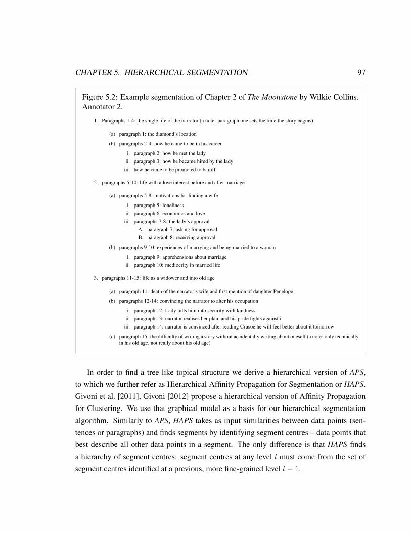
CHAPTER 5. HIERARCHICAL SEGMENTATION 97
Figure 5.2: Example segmentation of Chapter 2 of The Moonstone by Wilkie Collins.Annotator 2.
1. Paragraphs 1-4: the single life of the narrator (a note: paragraph one sets the time the story begins)
(a) paragraph 1: the diamond’s location
(b) paragraphs 2-4: how he came to be in his career
i. paragraph 2: how he met the ladyii. paragraph 3: how he became hired by the lady
iii. how he came to be promoted to bailiff
2. paragraphs 5-10: life with a love interest before and after marriage
(a) paragraphs 5-8: motivations for finding a wife
i. paragraph 5: lonelinessii. paragraph 6: economics and love
iii. paragraphs 7-8: the lady’s approvalA. paragraph 7: asking for approvalB. paragraph 8: receiving approval
(b) paragraphs 9-10: experiences of marrying and being married to a woman
i. paragraph 9: apprehensions about marriageii. paragraph 10: mediocrity in married life
3. paragraphs 11-15: life as a widower and into old age
(a) paragraph 11: death of the narrator’s wife and first mention of daughter Penelope
(b) paragraphs 12-14: convincing the narrator to alter his occupation
i. paragraph 12: Lady lulls him into security with kindnessii. paragraph 13: narrator realises her plan, and his pride fights against it
iii. paragraph 14: narrator is convinced after reading Crusoe he will feel better about it tomorrow
(c) paragraph 15: the difficulty of writing a story without accidentally writing about oneself (a note: only technicallyin his old age, not really about his old age)
In order to find a tree-like topical structure we derive a hierarchical version of APS,to which we further refer as Hierarchical Affinity Propagation for Segmentation or HAPS.Givoni et al. [2011], Givoni [2012] propose a hierarchical version of Affinity Propagationfor Clustering. We use that graphical model as a basis for our hierarchical segmentationalgorithm. Similarly to APS, HAPS takes as input similarities between data points (sen-tences or paragraphs) and finds segments by identifying segment centres – data points thatbest describe all other data points in a segment. The only difference is that HAPS findsa hierarchy of segment centres: segment centres at any level l must come from the set ofsegment centres identified at a previous, more fine-grained level l − 1.

CHAPTER 5. HIERARCHICAL SEGMENTATION 98
This chapter is structured as follows. Section 5.2 formulates the underlying HAPS
model. Section 5.2.1 contains step-by-step derivation of the new update messages. Section5.3 describes the settings for the experimental evaluation of HAPS. And Section 5.4 reportsresults. In Section 5.6 we discuss some of the weaknesses of this approach and potentialavenues for its improvement.
The readers not interested in how the formulae are derived can safely skip section 5.2.1describing the derivation of the algorithm.
5.2 Formulating hierarchical Affinity Propagation for seg-mentation (HAPS)
We will start by defining a factor graph model for HAPS. The model described here closelyfollows the model for hierarchical clustering proposed by [Givoni, 2012], in particular themodel HAP-B. For the sake of completeness, we repeat a lot of the definitions from thatwork in this dissertation. However, we skip lengthy derivations that are identical to theHAP-B model (namely the derivation of the new responsibility messages) and refer thereader to [Givoni, 2012, p. 96-120, 160-172] for details.
Our objective is as follows. Given a sequence ofN data point (sentences or paragraphs)we wish to build a topical tree where top levels capture the most pronounced fluctuations oftopic in a document, and lower levels capture more fine-grained ones. Formally, we wishto find a hierarchy of segments such that segments higher up in the tree consist of smallersegments found at the lower levels of the tree. At each level of the tree, all data pointswill be assigned to segment centres. However, we impose a constraint that segment centresat the level l, l > 1 must be chosen from the set of of segment centres identified at thepreceding level l − 1.
The inputs for HAPS are quite similar to the inputs for APS. Assuming that one wishesto segment a sequence of N data points into a hierarchy of L levels, one needs to supplyHAPS withLmatrices of pairwise similarities between these points, {SIMl(i, j)}i,j∈{1,...,N}.Each matrix {SIMl(i, j)} defines similarities for a corresponding level l ∈ {1, . . . , L}. Itis possible (and indeed this is what we do in this work) to have a single matrix of similari-ties shared between levels, but the model allows additional flexibility. The matrices do not

CHAPTER 5. HIERARCHICAL SEGMENTATION 99
Figure 5.3: Factor graph for Hierarchical Affinity Propagation for Segmentation, HAPS.
Cl−11 Cl−1
i Cl−1N
el−11 el−1
i el−1N
El−11 Eil − 1 El−1
N
Il−11
Il−1i
Il−1N
cl−111 cl−1
1i cl−11N
cl−1i1 cl−1
ii cl−1iN
cl−1N1 cl−1
Ni cl−1NN
S11l−1 Sl−11i
S1Nl−1
Sl−1i1 Sl−1
ii Sl−1iN
Sl−1N1 Sl−1
Ni Sl−1NN
Level l -1
Cl1 Cl
j ClN
el1 elj elN
El1 El
j ElN
Il1
Ili
IlN
cl11 cl1j cl1N
cli1 clij cliN
clN1 clNj clNN
S11l Sl1j
S1Nl
Sli1 Sl
ij SliN
SlN1 Sl
Nj SlNN
Level l

CHAPTER 5. HIERARCHICAL SEGMENTATION 100
need to be fully specified, nor do they need to be symmetric.The second type of input are preferences, vectors of self-similarities which reflect a
priori beliefs of how likely each data point is to be selected as a segment centre. For amodel with L layers one needs to supply L vectors P l = pl1, ...p
lN where each value pli
reflects a priori belief of how likely the point i is to be chosen as a segment centre in thelayer l. Because preferences are also the only parameter that controls the granularity ofsegmentation, these values need to differ between levels, with higher values correspondingto more segments (suitable for bottom levels) and lower values corresponding to fewersegments (suitable for top-level segments). In this work, we set preferences to the samevalue within levels, effectively making all sentence equally likely candidates to be segmentcentres. However, more intelligent settings may improve the quality of segmentations.
Figure 5.3 shows a factor graph corresponding to the HAPS model. It looks quite similarto the model for APS (Chapter 4, Figure 4.2) with several important differences. The factorgraph contains layers corresponding to the levels of segmentation. In Figure 5.3 the levell on the right-hand side of the picture corresponds to a higher, more coarse-grained levelin the topical tree. The level on the left, l − 1, is a more fine-grained level. The bottomnode in this notation is always l = 1. Two adjacent levels l and l − 1 are connected byedges between factor nodes I li at level l and corresponding variable nodes el−1i at the lowerlevel l− 1. Please note that in our new notation the superscripts on both factor and variablenodes denote the layer from which node comes.
Recall that the dark rectangular nodes are factor (or function) nodes. They encodea function on variables that are connected to them. The light circles are variable nodes.In the HAPS model, all variable are binary. By running the max-sum algorithm, we canobtain a configuration that maximizes that sum of all of the component functions (encodedas factor nodes).
There are four types of factor nodes in Figure 5.3 : C, E, I , S. These functions reoccurat each level. Factors S and C encode similarities and preferences. Factors I and E areconstraint functions: they evaluate either to −∞ (for invalid configurations) or to 0 (forvalid ones).
Let us look closer at Figure 5.3. Just like in APS, variable nodes clij are binary. Ifclij = 1 then the point i is assigned to the segment centred around point j in the level l ofthe hierarchy. Conversely, if clij = 0 then j is not the segment centre for the point i in the

CHAPTER 5. HIERARCHICAL SEGMENTATION 101
level l.There are two main differences between HAPS and the flat APS model. First of all,
factor nodes I li at each level are connected to the variable nodes el−1i in the previous level,carrying information across levels. Secondly, there are new variable nodes, elj , and thenodes elj are in turn connected to new factor nodes C l
j . The new variables elj are binary.They explicitly capture if the point j is chosen to be a segment centre in the level l. There-fore elj = 1 iff there is a segment around j in the level l. Otherwise elj = 0.
Factor nodes C lj explicitly capture preference values at the level l. C l
j(elj = 1) = pl(j)
(the preference value of data point j in level l) and C lj(e
lj = 0) = 0. Recall that in the
flat APS model, preferences were captured by the Sjj factor nodes on the diagonal of themodel. In the HAPS model, for all ∀j, l, Sljj = 0 and preferences are captured by the C l
j
factors.Now let us describe in detail the factor nodes.Similarly to APS, Slij factor nodes encode user-defined similarities between data points
and candidate segment centres. (SIMl(i, j) is the similarity between points i and j in thelevel l of segmentation hierarchy):
Slij(clij) =
SIMl(i, j) if clij = 1
0 otherwise(5.1)
Factor nodes C lj(e
lj) are new in this model. They encode preferences (self-similarities)
for data points at each level l: if a data point j is chosen to be a segment centre at a givenlevel, then C l
j(elj) evaluates to plj (preference of j at the level l), otherwise its value is 0.
C lj(e
lj) =
plj if elj = 1
0 otherwise(5.2)
In the flat APS model an I factor node encodes a single-segment constraint: each datapoint must belong to exactly one segment (and therefore be assigned to exactly one seg-ment centre). In the HAPS model I factors also encode relationships between levels of thehierarchy. At any given level l > 1, a data point j may be chosen to be a segment centre ifand only if it was chosen to be a segment centre in the previous level:
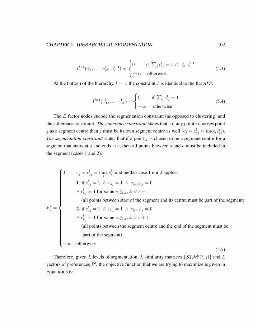
CHAPTER 5. HIERARCHICAL SEGMENTATION 102
I l>1i (cli1, . . . , c
liN , e
l−1i ) =
0 if∑
j clij = 1, clii ≤ el−1i
−∞ otherwise(5.3)
At the bottom of the hierarchy, l = 1, the constraint I is identical to the flat APS:
I l=1i (c1i1, . . . , c
1iN) =
0 if∑
j c1ij = 1
−∞ otherwise(5.4)
The E factor nodes encode the segmentation constraint (as opposed to clustering) andthe coherence constraint. The coherence constraint states that a if any point i chooses pointj as a segment centre then j must be its own segment centre as well (elj = cljj = maxi c
lij).
The segmentation constraint states that if a point j is chosen to be a segment centre for asegment that starts at s and ends at e, then all points between s and e must be included inthe segment (cases 1 and 2).
Elj =
0 elj = cljj = maxiclij and neither case 1 nor 2 applies
1. if cljj = 1 ∧ csj = 1 ∧ c(s−1)j = 0
∧ clkj = 1 for some s ≤ j, k < s− 1
(all points between start of the segment and its centre must be part of the segment)
2. if cljj = 1 ∧ cej = 1 ∧ c(e+1)j = 0
∧ clkj = 1 for some e ≥ j, k > e+ 1
(all points between the segment centre and the end of the segment must be
part of the segment)
−∞ otherwise(5.5)
Therefore, given L levels of segmentation, L similarity matrices {SIMl(i, j)} and Lvectors of preferences P l, the objective function that we are trying to maximize is given inEquation 5.6:

CHAPTER 5. HIERARCHICAL SEGMENTATION 103
max{clij},{elj}
S({clij}, {elj}) =∑i,j,l
Sli,j(clij) +
∑i,l
I li(cli1, . . . , c
liN , e
l−1i ) (5.6)
+∑j,l
Elj(c
l1j, . . . , c
lNj, e
lj) +
∑j,l
C lj(e
lj)
Intuitively, we are trying to find a configuration of variables that maximizes the sum ofsimilarities of all data points and their respective segment centres for all layers, plus the sumof preferences for all segment centres subject to the constraints of coherence, segmentationand hierarchical structure.
5.2.1 Update messages for HAPS
This section contains step-by-step derivation of the new update messages for HAPS. Weskip the derivation of the new responsibility messages because the process is lengthy andidentical to the HAP-B model by [Givoni, 2012, pp. 168-172].
Figure 5.4 shows a close-up of all message types in the graph.Recall that a message from a variable to a function is computed as the sum of all in-
coming messages, except for the message from the recipient node:
µx→f =∑
f ′∈N(x)\f
µf ′→x (5.7)
N(x) is the set of all function nodes which are x’s neighbours. The message reflects theevidence about the distribution of x from all functions which have x as an argument, exceptfor the function corresponding to the receiving node f .
A message µf→x from function f to variable x is computed as follows:
µf→x = maxN(f)\x
(f(x1, . . . , xm) +∑
x′∈N(f)\x
µx′→f ) (5.8)
N(f) is the set of all variable nodes which are f ’s neighbours. The message reflects theevidence about the distribution of x from the function f and its neighbours other than x.
Looking at Figure 5.4 we can see there are ten types of messages: α, ρ, φ, τ, p, p, µ, η, β

CHAPTER 5. HIERARCHICAL SEGMENTATION 104
Figure 5.4: Message types sent in the HAPS model.
and s. Messages α, ρ, p, p, µ, η, β and s are intra-level ones while τ and φ carry informationacross levels.
αlij and ρlij messages circulate between variable nodes clij and function nodes Elj . Mes-
sages βlij and ηlij are sent between variable nodes clij and function nodes I li within levell. There are also messages µlj and plij sent between El
j and elj . While we use the val-ues of these messages in our computations, they do not need to be sent explicitely as theyare subsumed by other messages (see below). Messages slij and plj evaluate either to 0 orto the value of either SIMl(i, j) or plj respectively (similarity between points i and j orpreference value for point j in the level l).
The inter-layer messages are φ and τ .φl−1i is sent from the factor node I li to the variable node el−1i in the preceding level l−1.
For clarity, we refer to the messages going from level l to l − 1 as φl−1 and we refer to themessages incoming to level l as φl. In essence, φl−1i are messages that ‘tell’ lower levelsabout the distribution of variables from upper levels.
τ l+1j is sent from a variable node elj in the level l to the factor node I l+1
i of the following
level l + 1. With τ messages, we refer to the upward-going messages as τ l+1j and to the
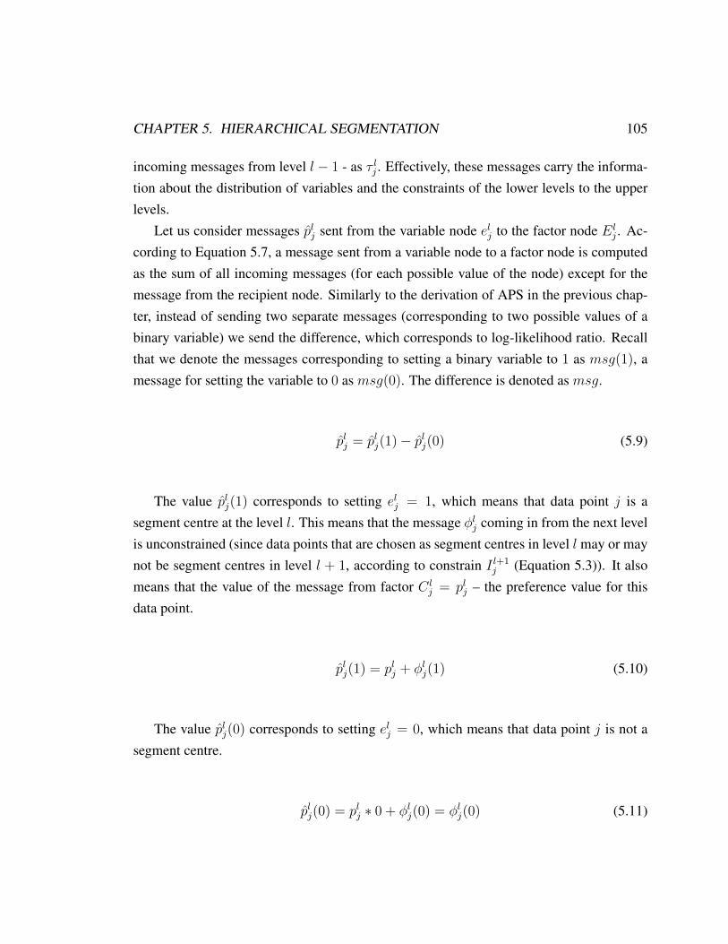
CHAPTER 5. HIERARCHICAL SEGMENTATION 105
incoming messages from level l − 1 - as τ lj . Effectively, these messages carry the informa-tion about the distribution of variables and the constraints of the lower levels to the upperlevels.
Let us consider messages plj sent from the variable node elj to the factor node Elj . Ac-
cording to Equation 5.7, a message sent from a variable node to a factor node is computedas the sum of all incoming messages (for each possible value of the node) except for themessage from the recipient node. Similarly to the derivation of APS in the previous chap-ter, instead of sending two separate messages (corresponding to two possible values of abinary variable) we send the difference, which corresponds to log-likelihood ratio. Recallthat we denote the messages corresponding to setting a binary variable to 1 as msg(1), amessage for setting the variable to 0 as msg(0). The difference is denoted as msg.
plj = plj(1)− plj(0) (5.9)
The value plj(1) corresponds to setting elj = 1, which means that data point j is asegment centre at the level l. This means that the message φlj coming in from the next levelis unconstrained (since data points that are chosen as segment centres in level l may or maynot be segment centres in level l + 1, according to constrain I l+1
j (Equation 5.3)). It alsomeans that the value of the message from factor C l
j = plj – the preference value for thisdata point.
plj(1) = plj + φlj(1) (5.10)
The value plj(0) corresponds to setting elj = 0, which means that data point j is not asegment centre.
plj(0) = plj ∗ 0 + φlj(0) = φlj(0) (5.11)

CHAPTER 5. HIERARCHICAL SEGMENTATION 106
Taking the difference between 5.10 and 5.11 we get:
plj = plj + φlj (5.12)
Now let us consider message µlj going from the factor node Elj to the variable node elj .
According to Equation 5.8, a message from a factor node to a variable node corresponds tothe maximum value of the sender function plus the sum of all incoming messages.
The case where elj = 0 means that means that data point j is not segment centre andtherefore it cannot exemplify any other data points. Otherwise, the constraint Ej is violatedand the function evaluates to −∞. The only valid configuration is to set all clij = 0,∀i:
1 j N
The picture graphically shows a valid configuration. However, keep in mind that thevalue of µj depends on the column j, not the row j. The picture is only horizontal tosimplify the layout of this dissertation.
µlj(0) = ρjj(0) +∑i 6=j
ρij(0) (5.13)
In Equation 5.13 we factor out ρjj(0) only so as to simplify the following subtraction,otherwise it could have been under the summation sign.
If elj = 1, it means that data point j is a segment centre and there is a segment startingat some point s ≤ j and ending at some point e ≥ j:
1 s j e N

CHAPTER 5. HIERARCHICAL SEGMENTATION 107
µlj(1) = ρljj(1) +j
maxs=1
[s−1∑k=1
ρkj(0) +
j−1∑k=s
ρkj(1)] +N
maxe=j
[e∑
k=j+1
ρkj(1) +N∑
k=e+1
ρkj(0)]
(5.14)
Subtracting Equation 5.13 from Equation 5.14 we get:
µlj = ρljj +j
maxs=1
[
j−1∑k=s
ρkj] +N
maxe=j
[e∑
k=j+1
ρkj(1)] (5.15)
Next we derive upward going τ l+1j messages sent from variable nodes elj at level l to
function nodes I l+1j at level l + 1.
If elj = 1 (corresponding to τjl+1(1)) then:
τjl+1(1) = plj(1) + µlj(1) (5.16)
τjl+1(0) = plj(0) + µlj(0) (5.17)
Subtracting Equation 5.17 from Equation 5.16 we get:
τjl+1 = plj + µlj (5.18)
Substituting 5.15 in Equation 5.18 we get:

CHAPTER 5. HIERARCHICAL SEGMENTATION 108
τ l+1j = pl(j) + ρljj +
jmaxs=1
(
j−1∑k=s
ρlkj) +N
maxe=j
(e∑
k=j+1
ρlkj) (5.19)
Please note that there is no need to send messages µ explicitly as the necessary infor-mation is incorporated directly in terms of ρ messages in Equation 5.19.
Next, we turn our attention to the downward-going φl−1i messages, sent from the factornode I li at the level l to variable nodes el−1j at the level l − 1. According to the constraintI , only data points selected to be segment centres at the lower level may be selected tobe segment centres at the current level. Additionally, I li requires that each data point i beassigned to exactly 1 segment centre j in each level l (translating into the fact that for anyrow i,
∑cij = 1).
φl−1i (1) corresponds to setting el−1j = 1. This means that at this level, l, we only needto satisfy the one-out-of-all constraint (since if i is a segment centre at the level l−1 it mayor may not be a segment centre at the level l):
φl−1i (1) = maxk
(βlik(1) +∑t6=k
βlit(0)) (5.20)
If, on the other hand, el−1j = 0, then the data point j cannot be chosen to be a segmentcentre at the level l (βljj = 0). However, the one-out-of-all constraint must still be satisfied:
φl−1i (0) = βlii(0) + maxk 6=i
(βlik(1) +∑t6=k
βitl(0)) (5.21)
It is easier to take the difference between 5.20 and 5.21 if we re-write 5.20 as a maxi-mum of two cases (if point i is not a segment centre at the level l or if it is one):

CHAPTER 5. HIERARCHICAL SEGMENTATION 109
φl−1i (1) = maxk
(βlik(1) +∑t6=k
βitl(0)) = (5.22)
max[βlii(0) + maxk 6=i
(βlik(1) +∑t6=k
βitl(0)), βlii(1) +∑k 6=i
βlik(0)]
Now we can take the difference between Equations 5.22 and 5.21 using two facts: 1)max(x, y)− x = max(0, y − x) and 2) βlij = slij + αlij:
φl−1i = max[βlii(0) + maxk 6=i
(βlik(1) +∑t6=k
βitl(0)), βlii(1) +∑k 6=i
βlik(0)]− (5.23)
− [βlii(0) + maxk 6=i
(βlik(1) +∑t6=k
βitl(0))] =
= max[0, αii −maxk 6=i
(slij + αlij)]
φl−1i = max[0, αii −maxk 6=i
(slik + αlik)] (5.24)
Next we will derive the availability messages αlij sent within level l from factor nodeElj to variable node clij . The derivation of these messages is almost identical to that in the
flat version of APS. The only difference is that factor nodes Elj have one more incoming
message that needs to be taken into account, namely plj . Just as before, we need to considerthree cases: 1) i = j 2) i < j and 3) i > j.
If i = j we need to take the difference between the following configurations (whichcorresponds to taking the difference between Equations 5.25 and 5.26):
1 s j e N
1 j N

CHAPTER 5. HIERARCHICAL SEGMENTATION 110
αljj(1) = plj(1) +j
maxs=1
[s−1∑k=1
ρkj(0) +
j−1∑k=s
ρkj(1)] +N
maxe=j
[e∑
k=j+1
ρkj(1) +N∑
k=e+1
ρkj(0)]
(5.25)
Note that we use the value of plj corresponding to setting elj = 1 because if there is asegment centred around j, elj must be 1, according to the constraint E. Conversely, if thereis no segment, then elj = 0 and all other variables (clij) must be set to 0 as well:
αljj(0) = plj(0) +∑i 6=j
ρij(0) (5.26)
Taking the difference and substituting plj = plj + φlj we get:
αljj = plj +j
maxs=1
(
j−1∑k=s
ρkj) +N
maxe=j
(e∑
k=j+1
ρkj) (5.27)
αljj = plj + φlj +j
maxs=1
(
j−1∑k=s
ρkj) +N
maxe=j
(e∑
k=j+1
ρkj)
Please note that by using the equality plj = plj + φlj we eliminate the need to explicitlycompute or send p messages.
Next, let us consider the case where i < j. If clij = 1, then there must a segment centredaround j. This means that cljj = 1 and elj = 1 :
1 s i j e N

CHAPTER 5. HIERARCHICAL SEGMENTATION 111
αij, i<j(1) = plj(1) +i
maxs=1
[s−1∑k=1
ρlkj(0) +i−1∑k=s
ρlkj(1)] +
j−1∑k=i+1
ρlkj(1) + ρljj(1)+ (5.28)
+N
maxe=j
[e∑
k=j+1
ρlkj(1) +N∑
k=e+1
ρlkj(0)]
If, on the other hand, clij = 0 then there are two possibilities. There may be a segmentaround j but it starts after i (Equation 5.29) or there may be no segment around j (Equation5.30). The former case correspond to:
1 i s j e N
αlij(0) = plj(0) +i−1∑k=1
ρkj(0) +j
maxs=i+1
[s−1∑k=i+1
ρkj(0) +
j−1∑k=s
ρkj(1)]+ (5.29)
ρjj(1) +N
maxe=j
[e∑
k=j+1
ρkj(1) +N∑
k=e+1
ρkj(0)]
In the second case (if there is no segment centred around j at this level) we have:
1 i j N
αljj(0) = plj(0) +∑i 6=j
ρij(0) + ρjj(0) (5.30)
Taking the difference we get an equation much like that in the flat APS:
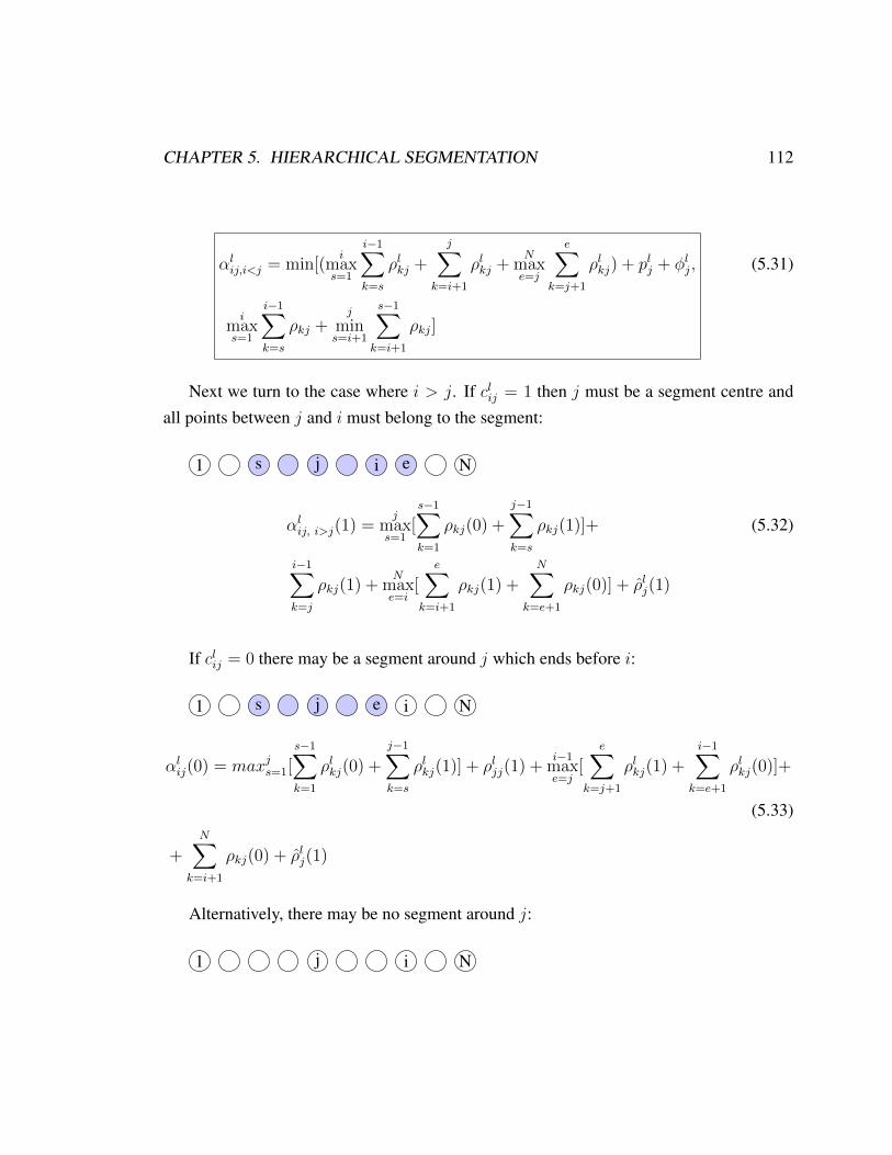
CHAPTER 5. HIERARCHICAL SEGMENTATION 112
αlij,i<j = min[(i
maxs=1
i−1∑k=s
ρlkj +
j∑k=i+1
ρlkj +N
maxe=j
e∑k=j+1
ρlkj) + plj + φlj,
imaxs=1
i−1∑k=s
ρkj +j
mins=i+1
s−1∑k=i+1
ρkj]
(5.31)
Next we turn to the case where i > j. If clij = 1 then j must be a segment centre andall points between j and i must belong to the segment:
1 s j i e N
αlij, i>j(1) =j
maxs=1
[s−1∑k=1
ρkj(0) +
j−1∑k=s
ρkj(1)]+ (5.32)
i−1∑k=j
ρkj(1) +N
maxe=i
[e∑
k=i+1
ρkj(1) +N∑
k=e+1
ρkj(0)] + ρlj(1)
If clij = 0 there may be a segment around j which ends before i:
1 s j e i N
αlij(0) = maxjs=1[s−1∑k=1
ρlkj(0) +
j−1∑k=s
ρlkj(1)] + ρljj(1) +i−1maxe=j
[e∑
k=j+1
ρlkj(1) +i−1∑
k=e+1
ρlkj(0)]+
(5.33)
+N∑
k=i+1
ρkj(0) + ρlj(1)
Alternatively, there may be no segment around j:
1 j i N

CHAPTER 5. HIERARCHICAL SEGMENTATION 113
αlij(0) =∑k/∈i,j
ρlkj(0) + +ρlj(0) (5.34)
Taking the difference we get:
αlij,i>j = min[(j
maxs=1
j−1∑k=s
ρlkj +i−1∑k=j
ρlkj +N
maxe=i
e∑k=i+1
ρlkj) + plj + φlj,
i−1mine=j
i−1∑k=e+1
ρlkj +N
maxe=i
e∑k=i+1
ρlkj]
(5.35)
The top level of the hierarchy, l = L is not connected to another higher level and thereare no incoming φ messages. Because of that the availability messages at the level l = L
are identical to those of APS.The responsibility messages in HAPS are identical to the responsibility messages in
HAP [Givoni, 2012, pp. 168-171]. The derivation of these messages follows the samelogic as all other messages explained here. It relies on the fact that ρlij = slij + ηlij andβlij = slij + αlij . We will not repeat these lengthy derivations here. The final equations areas follows:
If i = j then:
ρl,l>1ii = min(0, τ li )−max
k 6=i(slik + αlik) (5.36)
If i 6= j then:
ρl,l>1ij = slij +min[max(0,−τ li )− αlii,−max
k*i,j(slik + αlik)] (5.37)
It should be noted that at the bottom level of the hierarchy, l = 1, the I factors are notconnected to e variables from the previous level (as there is no previous level). Therefore,

CHAPTER 5. HIERARCHICAL SEGMENTATION 114
at the level l = 1 the responsibility messages are identical to those of APS:
ρl,l=1ij = s1ij −max
k 6=j(s1ik + αik) (5.38)
The pseudo-code for HAPS is shown in Algorithm 2.The computational properties of HAPS are similar to those of the flat version. On each
iteration, we need to send L ×M × N messages where L is the number of levels in thehierarchy, M ≤ N is the size of the sliding window used to compute similarities and N isthe total number of data points (sentences or paragraphs). So the computational complexityis O(MNL). The algorithm is easy to parallelize because the computation of messages foreach column (or row) is independent of other columns (or rows).
The messages still need to be dampened to avoid overshooting and oscillation:
newMsg = λ ∗ oldMsg + (1− λ)newMsg (5.39)
We used a dampening factor λ, 0.5 ≤ λ < 1. In practice, HAPS appears to be ratherinsensitive to the values of λ. We used λ = 0.95 for most experiments.
In our experiments we have tried two message-passing schedules: the flooding scheduledescribed in the previous chapter and also a different schedule suggested by [Givoni, 2012].When using the flooding schedule, for each level of the hierarchy, we iteratively send φ,ρ, α and τ messages. When using Givoni’s schedule, the intra-level messages are sent 10times within each level and only then the upward going τ message are sent once. Theprocedure is propagated all the way up the hierarchy and is repeated going downward.During preliminary experiments we found that the results were identical for both schedulesbut the latter schedule took significantly longer to converge. Because of that all results arereported using the flooding schedule.

CHAPTER 5. HIERARCHICAL SEGMENTATION 115
Algorithm 2 Hierarchical Affinity Propagation for Segmentation
1: input: 1) a set of pairwise similarities {SIM(i, j)}(i,j)∈{1,...,N}2 , SIM(i, j) ∈ R; 2)a set of preferences (self-similarities) {SIM(i, i)}i∈{1,...,N} indicating a priori likeli-hood of point i being a segment centre
2: initialization: ∀i, j : αij = 0 (set all availabilities to 0)3: repeat4: iteratively update responsibilities (ρ) and availabilities (α)5:
∀i, l : φl−1i = max[0, αii −maxk 6=i
(slik + αlik)]
6:
∀i, j, l : ρlij =
min(0, τ li )−max
k 6=i(slik + αlik) if i = j
slij +min[max(0,−τ li )− αlii,−maxk*i,j
(slik + αlik)] if i 6= j
7:
∀i, j, l : αlij =
plj + φlj +j
maxs=1
(
j−1∑k=s
ρlkj) +N
maxe=j
(e∑
k=j+1
ρlkj) if i = j
αlij,i<j = min[(i
maxs=1
i−1∑k=s
ρlkj +
j∑k=i+1
ρlkj +N
maxe=j
e∑k=j+1
ρlkj) + plj + φlj,
imaxs=1
i−1∑k=s
ρlkj +j
mins=i+1
s−1∑k=i+1
ρlkj] if i < j
min[(j
maxs=1
j−1∑k=s
ρlkj +i−1∑k=j
ρlkj +N
maxe=i
e∑k=i+1
ρlkj) + plj + φlj,
i−1mine=j
i−1∑k=e+1
ρlkj +N
maxe=i
e∑k=i+1
ρlkj]
8:
∀j, l : τ l+1j = pl(j) + ρljj +
jmaxs=1
(
j−1∑k=s
ρlkj) +N
maxe=j
(e∑
k=j+1
ρlkj)
9: until convergence10: compute the final configuration of variables: ∀i, j j is the segment centre for i iff
ρij + αij > 011: output: segment centre assignments

CHAPTER 5. HIERARCHICAL SEGMENTATION 116
5.3 Experimental setting
In this section we describe an experimental evaluation of HAPS.It was more difficult to evaluate the HAPS segmenter than the flat APS segmenter. Hier-
archical segmentation is far less explored than one-level topical segmentation and becauseof this it was difficult to find either comparable systems or evaluation metrics or benchmarkdatasets. In the experiments described in this section we did our best to evaluate the seg-menter and to appropriately position it within the context of related research given what isavailable in the public domain.
In order to see how sensible and useful are the topical trees produced by the HAPS
algorithm, we ran the system on two datasets annotated with hierarchical structure. Theonly comparable hierarchical segmenter [Eisenstein, 2009] is unfortunately not publiclyavailable at the time of writing. To gauge the performance of HAPS we compared the treesproduced by HAPS to those obtained by running two flat segmenters (Minimum Cut Seg-
menter and Bayesian Segmenter) iteratively. Both Minimum Cut Segmenter and Bayesian
Segmenter require ‘knowing’ the number of segments at each level in advance – which isnot a very realistic requirement for hierarchical segmentation: it is hard to know that num-ber even for a single level, let alone for each subsegment at each level. HAPS does notrequire this information (nor can it make any use of it if available), but through the use ofpreferences offers a degree of abstraction when choosing the granularity of segmentations.
We compared the performance of HAPS with two baselines (none of them a comparablehierarchical segmenter) using two evaluation metrics. The baselines consist of running theMinimum Cut Segmenter and the Bayesian Segmenter iteratively (first, to find the top levelsegment boundaries, then for each identified segment, we treat it as a separate documentand find its own internal ‘segments’). Normally, both the Minimum Cut Segmenter andthe Bayesian Segmenter have been designed for situations when the number of segmentsis known in advance. It is possible to run the Bayesian Segmenter without this parameter(though this is not the intended usage), however Minimum Cut Segmenter cannot be runwithout specifying the number of segments in advance. To allow fair comparison (sinceHAPS does not have access to this information) we ran the Bayesian Segmenter with andwithout specifying the number of segments and the Minimum Cut Segmenter only with thenumber of segments given. HAPS did not have access to the information about the number

CHAPTER 5. HIERARCHICAL SEGMENTATION 117
of segments.The results of the experiments suggest that HAPS performs comparably or slightly bet-
ter than the baseline segmenters with the number of segments specified. In the situationwhen the Bayesian Segmenter does not have access to the information about the number ofsegments, HAPS performs significantly better. However, it should be kept in mind that theevaluation metrics are severely limited in their perceptiveness.
Datasets. We have used two datasets to evaluate the performance of the HAPS seg-menter. The first one is the hierarchical Moonstone dataset described in detail in Section3.2. Recall that the dataset consists of nine chapters from The Moonstone annotated by 3-6people each. The average number of annotations per chapter is 4.8. The annotators wererequested to build topical trees corresponding to each chapter, briefly describing the con-tents of each segment. The resulting structure is similar to a hierarchical outline that canbe mapped back onto the text. An example annotation for Chapter 2 of the Moonstone canbe found in Figure 5.2 in the beginning of this Chapter. It is also important to rememberthat this dataset is segmented at the paragraph level. Therefore, in our experiments we alsowork with paragraphs.
The hierarchical Moonstone dataset is a very challenging dataset. The annotators them-selves remarked that the task was at times difficult and that they occasionally had troublefinalizing their decisions. Just like the flat Moonstone dataset it is a literary one, with manydigressions and a low rate of lexical repetition.
The second dataset is the hierarchical Wikipedia dataset compiled by Carroll [2010].The dataset consists of 66 Wikipedia articles. The hierarchical annotations were automat-ically derived from structure of the corresponding webpage for each article. The datasetis also rather challenging. For one thing, the structure contains more levels than the hier-archical Moonstone corpus. It was mentioned in Section 3.2.3 that the average depth ofsegmentation in the Moonstone dataset is 3.00 levels (std.dev. = 0.65). In the Wikipedia
dataset the average depth of the topical tree is 3.85 levels (std.dev. = 0.43). On the otherhand, the trees in the Moonstone corpus are broader, while in the Wikipedia dataset thereoften are long and narrow branches, or occasionally one comes across the top level nodesconsisting of one or two sentences (this often happens with the first introductory sentencesof the articles). The Wikipedia corpus is segmented at the level of individual sentences.
To simplify fine-tuning of the parameters and the interpretation of results, we trimmed

CHAPTER 5. HIERARCHICAL SEGMENTATION 118
the trees in the Wikipedia corpus to three levels. That is, we only load the three top (i.e., themost prominent) levels of segmentation. We also run HAPS and the baseline segmenters toproduce three-tier trees.
Baselines. To the best of our knowledge, there are no publicly available implementa-tions of hierarchical segmenters. A recent segmenter explicitly built to establish hierarchalstructure [Eisenstein, 2009] is no longer available at the time of writing this dissertation.
To see if there is any use in explicitly producing hierarchical topical trees, we havecompared the performance of HAPS against the results obtained by iteratively runningsingle-level segmenters. For example, to iteratively produce a hierarchical segmentation,we would run a flat segmenter requesting it to produce the gold-standard number of seg-ments in the coarsest level of the reference segmentation, then take the obtained segmentsand segment each one one more time, again requesting the segmenter to produce the refer-ence number of boundaries for each subsegment. This procedure would be repeated l − 1
times to produce a tree with l levels.The flat segmenters chosen for these experiments are Minimum Cut Segmenter and
Bayesian Segmenter. It should be noted that both baseline segmenters were effectivelygiven a lot more information than HAPS: at each level they were ‘told’ how many segmentsand subsegments there were in the reference segmentation. In many cases at lower levelsof the tree, providing this information determines the answer. This is especially true aboutthe leaves of the topical trees in the Moonstone dataset. In that dataset, described at thelevel of paragraph, the segmentations in the bottom level are very fine-grained, oftentimeseach paragraph is described as a separate segment. In such cases, providing the number ofsegments at the bottom level gives a very significant advantage to the segmenter.
HAPS, on the other hand, neither needs nor accepts the number of segments as a pa-rameter. Instead, the values of the preferences specify a more abstract parameter: thegranularity of segmentation at each level.
In order to allow fair comparison, we compared the trees produced by HAPS to thetrees produced by the Bayesian Segmenter under two different conditions: with and with-out knowing the number of segments in advance. It should be noted that the Bayesian
Segmenter was designed and tested in a situation when it had access to this information.It is not possible to start the Minimum Cut Segmenter without specifying the number ofsegments, so all trees produced by that segmenter were produced having access to the in-
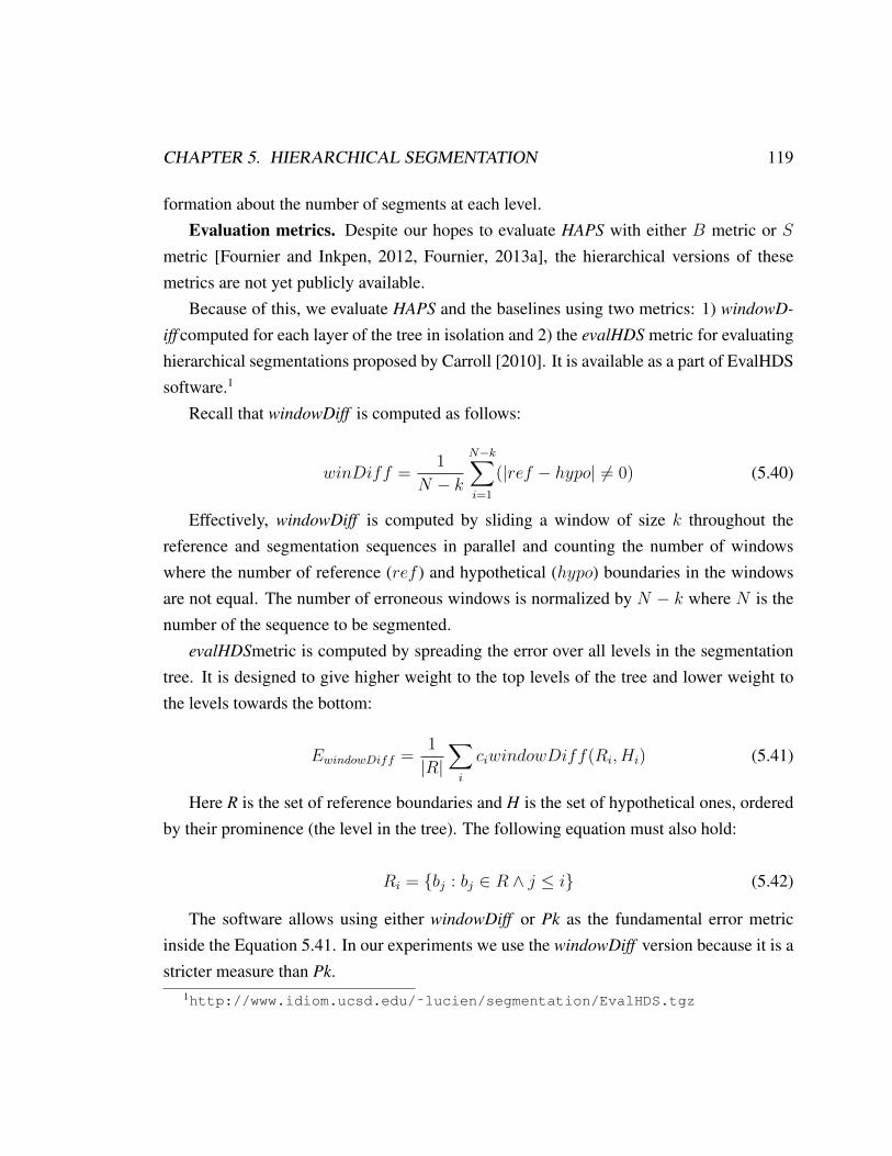
CHAPTER 5. HIERARCHICAL SEGMENTATION 119
formation about the number of segments at each level.Evaluation metrics. Despite our hopes to evaluate HAPS with either B metric or S
metric [Fournier and Inkpen, 2012, Fournier, 2013a], the hierarchical versions of thesemetrics are not yet publicly available.
Because of this, we evaluate HAPS and the baselines using two metrics: 1) windowD-
iff computed for each layer of the tree in isolation and 2) the evalHDS metric for evaluatinghierarchical segmentations proposed by Carroll [2010]. It is available as a part of EvalHDSsoftware.1
Recall that windowDiff is computed as follows:
winDiff =1
N − k
N−k∑i=1
(|ref − hypo| 6= 0) (5.40)
Effectively, windowDiff is computed by sliding a window of size k throughout thereference and segmentation sequences in parallel and counting the number of windowswhere the number of reference (ref ) and hypothetical (hypo) boundaries in the windowsare not equal. The number of erroneous windows is normalized by N − k where N is thenumber of the sequence to be segmented.
evalHDSmetric is computed by spreading the error over all levels in the segmentationtree. It is designed to give higher weight to the top levels of the tree and lower weight tothe levels towards the bottom:
EwindowDiff =1
|R|∑i
ciwindowDiff(Ri, Hi) (5.41)
Here R is the set of reference boundaries and H is the set of hypothetical ones, orderedby their prominence (the level in the tree). The following equation must also hold:
Ri = {bj : bj ∈ R ∧ j ≤ i} (5.42)
The software allows using either windowDiff or Pk as the fundamental error metricinside the Equation 5.41. In our experiments we use the windowDiff version because it is astricter measure than Pk.
1http://www.idiom.ucsd.edu/˜lucien/segmentation/EvalHDS.tgz

CHAPTER 5. HIERARCHICAL SEGMENTATION 120
Both windowDiff and evalHDS are less than ideal metrics for evaluating hierarchicalsegmentations because in both cases each level of the tree is viewed and evaluated in com-plete isolation from its neighbours. It would be far more insightful if we could evaluatesegmenters taking into account all levels of the tree. It would be good to distinguish the er-rors of omission (the segmenter completely missed a reference boundary) from the error ofsubstitution (a segmenter missed a boundary in the correct level, but placed it in an adjacentone). The hierarchical version of the S metric promised such analysis but, unfortunately, itis not yet publicly available.2
In the Moonstone dataset, each chapter is annotated by 3-6 people. It is not obvioushow to combine all available annotations into a gold standard for each chapter. For flatdatasets, it is customary to use the majority opinion as a judgement. However, it is lessthan ideal in this situation. As we have pointed out in Section 3.2.3, people disagree lessabout the presence/absence of a segment boundary than they disagree about its prominence- what level it should be at. Because of this, we felt that taking the majority opinion foreach level did not make much sense. When evaluating the performance of HAPS and thebaselines on the Moonstone dataset we compared the hypothetical segmentations againsteach available annotation and used the average value of the metric across all annotationsto select the best parameters. The results reported in the next section are computed in thesame manner.
We did our best to obtain a realistic picture of the results, but each metric has its short-comings. We compared topical trees using windowDiff and evalHDS [Carroll, 2010]. Bothmetrics are penalties: the higher the values, the worse the hypothetical segmentation. eval-
HDS computes windowDiff for each level of the tree in isolation and weighs the errorsaccording to their prominence in the tree. We computed evalHDS using the publicly avail-able Python implementation [Carroll, 2010]. When working with the Moonstone dataset,we realized that the software produces very low values, almost too good to be true. Thatis because the bottommost annotations are very fine-grained. Sometimes each paragraphcorresponds to a separate segment. This causes problems for the software. So, when wereport evalHDS values for the Moonstone dataset, we only consider two top levels of the
2We chose not to use single-level versions of either S or B in the same manner as we used windowDiff.Using these versions would not have circumvented the disadvantage of viewing each level in isolation fromits neighbours. Neither of the metrics has been used very widely and the results would have been difficult toposition within the community without providing much additional insight.

CHAPTER 5. HIERARCHICAL SEGMENTATION 121
tree, disregarding the leaves. We also remove the “too good to be true” outliers, though the“bad” tail is left intact. We applied the same procedure to all three segmenters, only for theMoonstone dataset.
When computing windowDiff, we treated each level of the tree as a separate segmen-tation and compared each hypothetical level against a corresponding level in the referencesegmentation.
To ensure that evaluations are well-defined at all levels, we propagated the more pro-nounced reference breaks to lower levels (in both annotations and in the results). This wasdone to ensure that the whole sequence is segmented at each level. Otherwise windowD-
iff is not well-defined. Conceptually this means that if there is a topical shift of noticeablemagnitude (e.g. at the top level), there must be at least a shift of less pronounced magnitude(e.g., an an intermediate level).
Experimental design. We ran HAPS and the two iterative baselines on both availablehierarchical datasets. To simplify the analysis and because the average depth of manuallycreated trees in the Moonstone dataset is 3.00, we ran all segmenters so as to build three-tiertrees. An example tree produced by HAPS is shown in Figure 5.5. The text in this Figurecorresponds to the segment centres identified by HAPS. Of course, other segmenters do notidentify segment centres. The Figure shows only the top two levels of the tree since thebottom level of the tree contains six segments and, correspondingly, six paragraph-lengthsegment centres.
Bayesian Segmenter computes its own internal representation of documents. The rep-resentations used by both HAPS and Minimum Cut Segmenter are matrices of similaritiesbetween sentence or paragraphs in the input document. The default similarity metric is co-sine similarity (for details see the previous Chapter). We also ran both HAPS and Minimum
Cut Segmenter using STS-2012 similarity. It is computed in exactly the same manner as forthe flat APS (see the previous Chapter).
All segmenters are unsupervised and do not require training. However, Minimum Cut
Segmenter and HAPS benefit from a small development set to fine-tune the segmentationparameters. We evaluate the segmenters using a procedure similar to cross validation. Forn-fold cross-validation the corpus is randomly divided into n folds. Each fold contains atmost 3 development files and the rest of the fold is used for testing. The best parameters areautomatically selected using the development part of the fold. For HAPS the parameters

CHAPTER 5. HIERARCHICAL SEGMENTATION 122
Figure 5.5: Example topical tree produced by HAPS for Chapter 2 of The Moonstone.Two top levels.
1. Paragraphs 0-8. Segment centre:The woman I fixed my eye on, was the woman who kept house for me at my cottage. Hername was Selina Goby. I agree with the late William Cobbett about picking a wife. Seethat she chews her food well and sets her foot down firmly on the ground when she walks,and you’re all right. Selina Goby was all right in both these respects, which was onereason for marrying her. I had another reason, likewise, entirely of my own discovering.Selina, being a single woman, made me pay so much a week for her board and services.Selina, being my wife, couldn’t charge for her board, and would have to give me herservices for nothing. That was the point of view I looked at it from. Economy with adash of love. I put it to my mistress, as in duty bound, just as I had put it to myself.
(a) Paragraphs 0-3. Segment centre:I have omitted to state that I went with the bride to the bride’s husband’s house andlands down here. ”Sir John,” she says, ”I can’t do without Gabriel Betteredge.””My lady,” says Sir John, ”I can’t do without him, either.” That was his way withherand that was how I went into his service. It was all one to me where I went, solong as my mistress and I were together.
(b) Paragraphs 4-8. Segment centre:The woman I fixed my eye on, was the woman who kept house for me at my cottage.Her name was Selina Goby. [...]
2. Paragraphs 9-14. Segment centre:I received this magnificent present quite at a loss to find words to thank my mistress withfor the honour she had done me. To my great astonishment, it turned out, however, thatthe waistcoat was not an honour, but a bribe. My lady had discovered that I was gettingold before I had discovered it myself, and she had come to my cottage to wheedle me (ifI may use such an expression) into giving up my hard out-of-door work as bailiff, andtaking my ease for the rest of my days as steward in the house. I made as good a fightof it against the indignity of taking my ease as I could. But my mistress knew the weakside of me; she put it as a favour to herself. The dispute between us ended, after that, inmy wiping my eyes, like an old fool, with my new woollen waistcoat, and saying I wouldthink about it.

CHAPTER 5. HIERARCHICAL SEGMENTATION 123
are fine-tuned using exhaustive searching and Minimum Cut Segmenter chooses the bestparameters using a version of A* search.3
The parameters for HAPS can be roughly divided into two groups: parameters for com-puting the similarity matrix (e.g., smoothing parameters and the type of tf.idf metric to use- corpus or segment-based) and the segmentation parameters: dampening factor λ, prefer-ence values for each level of the tree and the size of the sliding window for the similaritymatrix. For the first group of parameters we use the experiments from Chapter 4 as a guideand reduce the search space by computing similarity matrices with the same parameters aswe used in the experiments in Section 5.4. HAPS segmenter turned out rather insensitiveto the value of λ as long as λ ≥ 0.8. We used the value λ = 0.95 in all experiments.
For preference values, preferences at the top of the tree must have lower values than atthe bottom of the tree because the lower the value of preferences, the fewer segments willbe identified at that level. The segmenter is quite sensitive to the fluctuations in preferencevalues for fine-grained segmentations (the values between the minimum and the medianvalue of similarities in the input matrix). However, it becomes less sensitive for near-zeroor negative preferences. This happens because HAPS and APS reply on the existence ofinformative segment centres to identify segment boundaries. If such representative datapoints cannot be found, then the segmenter is forced to choose “in the dark” – it mustassign data points to segment centres that are all equally bad at representing them. Effec-tively, this translates into the fact that it is rather difficult to force HAPS to produce fewersegments than it finds segment centres for past a certain point. In all our experiments,HAPS converged to a solution.
We used the regular flooding schedule of message passing in all experiments on hierar-chical segmentation.4
3Because of the naive search strategy that HAPS uses it effectively can only search a very small hypothesisspace, much smaller than the Minimum Cut Segmenter. This in one of the first items to correct in our futurework.
4In the preliminary experiments we also tried the schedule proposed by Givoni [2012]: sending 10 itera-tions of intra-level messages before sending upward going messages to the next level once and repeating thesame procedure going downward. But the results appeared to be the same, so we did not use this schedule inthe final experiments.

CHAPTER 5. HIERARCHICAL SEGMENTATION 124
Level Moonstone Wikipedia Moonstone WikipediawindowDiff windowDiff evalHDS evalHDS
HAPS3 (top) 0.337 (± 0.060) 0.421 (± 0.060) 0.353 0.4502 (middle) 0.422 (± 0.060) 0.447 (± 0.070) (± 0.072) (± 0.015)1 (bottom) 0.556 (± 0.070) 0.617 (± 0.080)
MinCutSeg-iter. 3 (top) 0.375 0.440 (± 0.075) 0.377 0.4442 (middle) 0.541 0.424 (± 0.064) (± 0.002) (± 0.002)
segm. known 1 (bottom) 0.601 0.471 (± 0.057)
BayesSeg-iter. 3 (top) 0.353 (± 0.071) 0.391 (± 0.070) 0.367 0.3702 (middle) 0.406 (± 0.053) 0.344 (± 0.033) (± 0.089) (± 0.019)
segm. known 1 (bottom) 0.504 (± 0.064) 0.354 (± 0.033)
BayesSeg-iter. 3 (top) 0.600 (± 0.071) 0.637 (± 0.070) 0.453 0.4372 (middle) 0.447 (± 0.053) 0.877 (± 0.033) (± 0.089) (± 0.022)
segm. unknown 1 (bottom) 0.545 (± 0.064) 0.952 (± 0.033)
Table 5.1: Evaluation of HAPS and iterative versions of Minimum Cut Segmenter andBayesian Segmenter using windowDiff per level and evalHDS
5.4 Experimental results and discussion
Table 5.1 shows the results of comparing HAPS with two baseline segmenters using win-
dowDiff and evalHDS. (In this Table the results are reported for the versions of HAPS
and Minimum Cut Segmenter that use simple cosine similarity matrices. The results usingSTS-2012 matrices are reported in Table 5.2.)
HAPS was run without knowing the number of segments. The Minimum Cut Segmenter
required that the exact number be specified. The Bayesian Segmenter was tested withand without that parameter. Therefore, rows 3 and 4 in Table 5.1 correspond to baselinesconsiderably more informed than HAPS. This is especially true about the bottom levelswhere sometimes knowing the exact number of segments unambiguously determines theonly possible segmentation.
The results suggest that HAPS performs well on the Moonstone dataset even when com-pared to more informed baselines. This applies to both metrics, windowDiff and evalHDS.Bayesian Segmenter performs slightly better at the bottom levels of the tree when it has theinformation about the exact number of segments. We hypothesize that the advantage maybe due to this additional information, especially when segmenting already small segmentsat level 1 into a predefined number of segments. Another explanation may be that whenusing windowDiff as the evaluation metric, HAPS was fine-tuned so as to maximize thevalue of windowDiff at the top level, effectively disregarding lower levels of segmentation.
On the Wikipedia dataset all segmenters perform worse. The informed version ofBayesian Segmenter performs best, but it is interesting to note a significant drop in per-

CHAPTER 5. HIERARCHICAL SEGMENTATION 125
Level Moonstone Wikipedia Moonstone WikipediawindowDiff windowDiff evalHDS evalHDS
HAPS-STS3 (top) 0.347 (± 0.05) 0.418 (±0.05) 0.359 0.5002 (middle) 0.532(± 0.012) 0.458 (±0.057) (± 0.078) (±0.023)1 (bottom) 0.584 (± 0.031) 0.743 (±0.101)
MinCutSeg-iter.-STS 3 (top) 0.401 0.441(± 0.071) 0.423 0.4892 (middle) 0.513 0.480 (±0.051) (± 0.046) (±0.034)
segm. known 1 (bottom) 0.584 0.479 (± 0.023)
Table 5.2: Evaluation of HAPS and iterative version of Minimum Cut Segmenter using STS-2012 matrices as input. The table reports windowDiff per level and evalHDS and standarddeviation.
formance when the number of segments is not specified.Overall HAPS appears to perform better than, or comparably to, the more informed
baselines, and much better than the baseline not given information about the number ofsegments. The results of HAPS are different with 95% confidence when compared to theuninformed Bayesian Segmenter baseline, but the differences with the more informed base-lines are not significant.
Looking at Table 5.2, it is somewhat surprising that using a more elaborate metric oftextual similarity, STS-2012, results in a palpable drop of performance. This is not entirelysurprising because the metric was not designed for topical segmentation per se. Becauseit is rather complex, it is hard to pin point what exactly causes this drop in performance.However, we hypothesize that this may be due to the fact that overall values of STS-2012
similarity are significantly higher than those of cosine similarity. This is because the metricleverages considerably more information about each sentence. In a way, everything is‘more similar’ when looking at it from the lens of STS-2012, especially considering thatin our case we are comparing sentences and paragraphs coming from the same sourcedocument. For example, because the sentences come from the same source, stylisticallythey all are likely to be very similar and stylistic similarity is a factor for STS-2012. Thisprobably results in overestimating topical similarity in many cases and ultimately, in worsesegmentations.

CHAPTER 5. HIERARCHICAL SEGMENTATION 126
5.5 Evaluating informativeness of the segment centres
Unlike the baselines segmenters, HAPS also identifies segment centres for each segmentand sub-segment. A segment centre provides a succinct summary of all other sentences orparagraphs in the segment. We decided to investigate if segment centres identified by HAPS
could be used as summaries. To this end, we compared the segment centres from the second(middle) level of the topical trees to automatically created summaries built using a recentautomatic summarizer CohSum [Smith et al., 2012]. Thorough evaluation of summariesis notoriously difficult and the results are preliminary. However, they suggest that HAPS
segment centres are rather indicative of the contents of the document.To compare the quality of the segment centres identified by HAPS and that of the sum-
maries created by CohSum we used the ROUGE metric [Lin, 2004].Data. In this experiment we used two datasets. The first dataset is the hierarchical
Moonstone dataset. The second dataset consists of 20 chapters from several novels by JaneAusten (further Austen corpus). We used chapters from the novels by the same author sothat preference values selected on a hold-out set would generalize well for the rest of thecorpus.
ROUGE software operates by comparing automatically built summaries against oneor more manually written gold-standard ones. Therefore, we needed manually writtensummaries for both the Moonstone and the Austen corpora. These gold-standard summarieswere downloaded from the SparkNotes website for each individual chapter.5
Evaluation metric. The basis of comparing the segment centres and the CohSum sum-maries was the publicly available Perl package ROUGE. ROUGE is the de facto evaluationstandard for research on automatic text summarization. ROUGE scores are computed bymeasuring several variations of n-gram overlap between the gold-standard summaries andthe candidate summaries produced by automatic summarizers. Effectively, a ROUGE scoreindicates how much lexical overlap there is between the candidate summary and the gold-standard summaries.
The ROUGE metric is popular due to its simplicity of use and availability for intermedi-ate evaluations. However, it has several disadvantages. First and foremost, lexical overlapis a rather distant approximation of the information content. While ROUGE scores have
5www.sparknotes.com/

CHAPTER 5. HIERARCHICAL SEGMENTATION 127
been shown to correlate with human judgements for news, there exists no such evidence forevaluating summaries of literature. Alternative methods of comparing summaries createdout of segment centres with the CohSum summaries could be asking human judges to readthe summaries, the chapters and to rate them on several counts. However, this would be arather expensive exercise. For now, we will restrict ourselves to using ROUGE and we willexplore more thorough methods of evaluating summaries in future work.
In our experiments we used ROUGE-1 and ROUGE-L variants of the ROUGE metric.We selected these variants because they are routinely used in the annual competitions oftext summarization systems – Text Analysis Conferences (TAC).
Baselines. We compared segment-centres based summaries to the summaries createdby the CohSum system. We chose this system because it is one of the very few recentsummarizers designed for single-document, not multi-document summarization and alsobecause of its competitive performance.
CohSum attempts to identify the most informative sentences in a document by takinginto account not only lexical information, but also the information about coreference linksbetween sentences. Sentences are treated as nodes in a graph, while coreferential expres-sions are treated as in-coming links. The system uses a version of PageRank algorithm[Brin and Page, 1998] to identify sentences that are central to the document.
Experimental design. In this experiment we used segment centres from the middlelevel in the topical trees. This choice is due to the fact that the bottom layer contains tomany segment centres and that the top layer may contain too few. This approximatelycorresponds to the 10% compression rate that we used for the CohSum system. The systemdoes not require fine-tuning parameters though it may benefit from a corpus to improveits estimation of inter-sentence similarities. We used the corpus based on Mary Shelley’sFrankenstein that was provided with the distribution. It is possible that a larger corpuswould improve the results.
Results. Table 5.3 shows the results of comparing CohSum summaries to the summariescomposed of segment centres identified by HAPS. While keeping in mind why ROUGE isnot a conclusive metric for evaluating summaries, it appears that the two types of sum-maries are rather comparable. Both ROUGE-1 and ROUGE-L scores are slightly higherfor segment-based summaries of the Moonstone corpus. The situation is reversed on theAusten corpus. However, the differences are very small. We interpret this as a sign that

CHAPTER 5. HIERARCHICAL SEGMENTATION 128
Moonstone corpus Austen corpusROUGE-1 ROUGE-L ROUGE-1 ROUGE-L
Segment centres 0.341 0.321 0.291 0.301(0.312, 0.370) (0.298, 0.346) (0.272, 0.311) (0.293, 0.330)
CohSum 0.294 0.269 0.305 0.307summaries (0.243, 0.334) (0.226, 0.306) (0.290, 0.320) (0.287, 0.327)
Table 5.3: HAPS segment centres compared to CohSum summaries: ROUGE scores and95% confidence intervals
segment centres identified by HAPS are rather indicative of the contents of the input docu-ments.
5.6 Conclusions
In this Chapter we presented an algorithm for hierarchical segmentation of documents.Given a sequence of n data points (sentences or paragraphs), HAPS takes as inputs thevalue L (the desired number of levels in the resultant tree), a matrix of pairwise similaritiesbetween data points and a preference value for each data point at each level. It outputssegment boundaries and segment centres for each level of the tree.
We could not find another publicly available hierarchical segmenter to compare withHAPS. Therefore, we compared the system with the results of running flat segmenters it-eratively. The baselines that we compared HAPS to were designed for situations when thenumber of segments to be found is known in advance – a rather unrealistic requirement forbuilding hierarchical structures. HAPS does not require this information and through theuse of preferences offers a level of abstraction when it comes to granularity of segmenta-tion. We think that this is a significant advantage.
Because the baselines were designed to “know” the desired number of segments inadvance, we compared HAPS to the trees built with and, when possible, without that infor-mation. The topical trees created by HAPS are comparable or slightly better than the treesbuilt by considerably more informed baselines. The HAPS trees are significantly betterthan the trees created by the Bayesian Segmenter when it had no access to the informationabout the number of segments at each level of the tree.
An additional advantage of using HAPS is that it also outputs segment centres. This

CHAPTER 5. HIERARCHICAL SEGMENTATION 129
effectively turns the topical trees into loose outlines, though it is rather likely that oftentimesthey may be not very coherent.
A Java implementation of HAPS will be made publicly available (it is currently avail-able upon request).
The HAPS segmenter also has several shortcomings and there is a lot of room for im-provement. One concern is the fact that the objective function is very centred on the seg-ment centres and on maximizing similarity between them and the data points found in eachsegment. This function does not take into account intra-segment similarity between datapoints as such, nor does it pay any attention to dissimilarity between segments. In futurework, it would be good to modify the objective function so as to take that information intoaccount. This may be especially useful for situations when the data points correspond toshort sentences, e.g., utterances in dialogues. In such situations, it may be difficult to findsentences that are descriptive of the whole segment in isolation if no other information istaken into account.
Other possible improvements are on-going. For now, during the fine-tuning stage HAPS
selects the best parameters by exhaustively searching the hypothesis space. This is rathercrude, as only a very small search space can be covered in this manner. It is almost cer-tain that the performance would be improved through using a more intelligent way to setparameters. We plan to do this in the near future.
From the definition of HAPS in Section 5.2, it can be seen that HAPS offers enoughflexibility to use different similarities for different levels of segmentation. In our currentexperiments, we have not explored this capability and used the same similarity matrix forall levels. It may be more intelligent to measure similarity differently for coarse-grainedand for fine-grained segmentations.
In a similar vein, we have not explored the flexibility of HAPS with regards to thepreference values. For each data point, at each level, the preference value specifies a priori
belief about how likely that data point is to be chosen as a segment centre at that level. Itwould make sense to give higher preference values to sentences that are longer, or, possibly,to sentences that have high concentration of character mentions, to name just a couple ofheuristics. Choosing good candidate segment centres may be a research area in and ofitself. We have not touched upon it in this work, but we plan to do so in the future.
A problem that was outside the scope of this dissertation is evaluation of hierarchical

CHAPTER 5. HIERARCHICAL SEGMENTATION 130
segmenters. In this research, we did our best to obtain an adequate picture of the HAPS
performance and to compare it to the baselines. However, the metrics that we have usedare not for tree-like structures by their nature, though they have been adapted to be usedon trees and not only on sequences. Neither windowDiff nor evalHDS takes into accountsimilarities and differences across different levels of the tree. Given our analysis of thehierarchical Moonstone corpus, such distinctions should be taken into account since evenfor manual segmentations a lion share of disagreements is not about the presence/absenceor about the precise location of a boundary, but about the prominence of a boundary in atopical tree.
To the best of our knowledge, apart from [Eisenstein, 2009] HAPS is the only publiclyavailable hierarchical segmenter. We think that hierarchical segmentation is a step up fromlinear segmentation in terms of informativeness and usability.

Chapter 6
Coreferential similarity
6.1 Introduction
In Chapters 4 and 5 we have described a flat and a hierarchical model for topical segmen-tation based on Affinity Propagation. Both algorithms rely on an already pre-computedmatrix of similarities between sentences. So far we have used two methods of measuringto what extent two passages are “about the same thing”: cosine similarity using a bag-of-words representation and a more competitive measure of similarity, that used in the winningsystem in the Semeval Semantic Textual Similarity track in 2012 (we refer to it as STS-2012
similarity). Both metrics use explicit surface information about tokens in the text to mea-sure how similar two sentences are. In this chapter, we try to improve upon these methodsof measuring similarity by taking into account referential expressions.
Most work on topical segmentation today revolves around the idea that if the topic ofdiscourse changes, so does the vocabulary [Youmans, 1991]. Indeed, by and large, intro-ducing new concepts almost necessarily requires that the concepts be named and described.However, how densely the concepts are explicitly mentioned, how often the mentions arerepeated depends to a large degree on the genre and on the cognitive complexity of thedocument. In scientific papers or legal documents clarity is paramount and the author goesto lengths stating things explicitly and avoiding ambiguity. However, the less complicatedthe document, the less it is necessary to explicitly repeat terminology. In literature, for ex-ample, word repetition is not only uncommon, it is usually a sign of bad writing. In casualconversations, the topic can easily be never mentioned explicitly. How can we identify
131

CHAPTER 6. COREFERENTIAL SIMILARITY 132
Figure 6.1: An excerpt from The Moonstone, Chapter 5.
[He]ent1 came back with a character that closed the doors of all hisent1 family againsthiment1, my lady (then just married) taking the lead, and declaring (with Sir John’sapproval, of course) that [her brother]ent1 should never enter any house of hers. Therewas more than one slur on [the Colonel]ent1 that made people shy of [him]ent1; but theblot of [the Diamond]ent2 is all I need mention here.
It was said [he]ent1 had got possession of [his Indian jewel]ent2 by means which,bold as [he]ent1 was, [he]ent1 didn’t dare acknowledge. [He]ent1 never attempted tosell [it]ent2–not being in need of money, and not (to give [him]ent1 his due again)making money an object. [He]ent1 never gave [it]ent2 away; [he]ent1 never even showed[it]ent2 to any living soul. Some said [he]ent1 was afraid of [its]ent2 getting [him]ent1
into a difficulty with the military authorities; others (very ignorant indeed of the realnature of [the man]ent1) said [he]ent1 was afraid, if [he]ent1 showed [it]ent2, of its costing[him]ent1 [his]ent1 life.
topical shifts in a document whose author does not “hold the reader’s hand”?It turns out that lexical cohesion (or, put simply, word repetition) is only one of several
devices of cohesion [Halliday and Hasan, 1976, p. 29]. Other possibilities are reference,substitution, ellipsis and conjunction. In this chapter we attempt to leverage referentialcohesion in order to estimate to what extent the topic remains constant between two sen-tences.
Figure 6.1 contains a short excerpt from The Moonstone. This example is annotated forthe presence of the two main entities that are the focus of the conversation – Colonel JohnHerncastle and the Moonstone. The name of the former is never mentioned, he is referredto mostly as he, the Colonel, the brother and the man. The text is highly cohesive and talksalmost exclusively about the Colonel and the jewel, yet there is almost no lexical repetition.Both APS and HAPS use only lexical information and would not be able to establish andleverage topical similarity between sentences in this example (the Minimum Cut Segmenter
and the Bayesian Segmenter would have the same problem). The same is true of the secondentity: the Moonstone is referred to as the Diamond, the jewel and it, and so a segmenterrelying only on lexical repetition would not be able to make much progress.
In general, a speaker/writer uses explicit vocabulary only to the extent that is necessary

CHAPTER 6. COREFERENTIAL SIMILARITY 133
for the message to get across and avoids unnecessary redundancy.1 If we replaced everyinstance of anaphoric reference to ent1 – Colonel John Herncastle – by the explicit mention,the result (shown in Figure 6.2) is annoying and is in fact difficult to understand.
Figure 6.2: An excerpt from The Moonstone, Chapter 5 with all references to ColonelJohn Herncastle made replaced by Colonel John Herncastle.
Colonel John Herncastle came back with a character that closed the doors of allColonel John Herncastle’s family against Colonel John Herncastle, my lady (thenjust married) taking the lead, and declaring (with Sir John’s approval, of course)that Colonel John Herncastle should never enter any house of hers. There was morethan one slur on Colonel John Herncastle that made people shy of Colonel JohnHerncastle; but the blot of the Moonstone is all I need mention here.
It was said Colonel John Herncastle had got possession of the Moonstone bymeans which, bold as Colonel John Herncastle was, Colonel John Herncastle didn’tdare acknowledge. Colonel John Herncastle never attempted to sell the Moonstone–not being in need of money, and not (to give Colonel John Herncastle his due again)making money an object. Colonel John Herncastle never gave the Moonstone away;Colonel John Herncastle never even showed the Moonstone to any living soul. Somesaid Colonel John Herncastle was afraid of the Moonstone getting Colonel JohnHerncastle into a difficulty with the military authorities; others (very ignorant indeedof the real nature of Colonel John Herncastle) said Colonel John Herncastle wasafraid, if Colonel John Herncastle showed the Moonstone , of its costing Colonel JohnHerncastle his life.
Lexical repetition is lower in texts that are cognitively less dense – fiction, every dayconversations, emails, etc. In technical texts, on the other hand, lexical repetition is neces-sary to ensure comprehension of concepts which are relatively involved. Since this researchproject is concerned with literary data, the question arises how we can measure topical sim-ilarity between sentences/paragraphs if lexical repetition does not seem to be too promisinga source. How can we make use of cohesion devices other than repetition, for example thedevices used in Figure 6.1?
An obvious answer would be to run an anaphora resolution system, and hopefully re-solve that he and the Colonel refer to John Herncastle and it and the jewel refer to theMoonstone. However, not only are anaphora resolution systems not very reliable yet, but
1See [Hoey, 1991] for a discussion of how lexical density relates to cognitive complexity.

CHAPTER 6. COREFERENTIAL SIMILARITY 134
also it would be somewhat of an overkill. Anaphora resolution is generally a rather com-plicated task requiring a lot of pre-processing. On the other hand, topical segmentation isa pre-processing task itself and running a complex system just to aid in pre-processing isinefficient. Additionally, it is known that anaphoric connections are restricted by the topicalstructure of a text [Kehler, 2002, p. 143–180], making the problem circular.
So, how can we make use of the pronoun he in Figure 6.1 without resolving it? Well, wecan safely assume that if an anaphoric expression is present (be it pronominal or nominal),it must refer to something. In other words, it almost necessarily signals a reference to apreviously mentioned entity – or to an entity somehow clear from the context.2 Therefore,for the purposes of establishing topical continuity, we do not need to resolve he in Figure6.1. By the virtue of simply encountering it we know that it refers to a nearby entity.
On the other hand, the noun phrase the Colonel also refers to something, and so doesthe man. How can we know whether the antecedent of a referring expression happensto occur in the preceding sentence, or further behind? It turns out that the syntactic typeof an anaphoric expression can tell us something about how accessible its referent is. Ingeneral, the less information is encoded in an anaphoric reference, the more accessible thereferent is [Givon, 1983]. For example, the referent of he should be more accessible thanthe referent of a proper noun phrase the Diamond. The notion of accessibility is complexand is influenced by the context, prominence and the number of potential antecedents, andseveral other factors. However, in written text, the distance between the referent and theantecedent is of primary importance. If we make a somewhat simplistic assumption of theother qualities being held equal, we can reasonably expect that the form of an anaphoricexpression is correlated with how far its antecedent is. By using this information, wecan model topical similarity of text using anaphoric expressions without actually resolvingthem.
The idea that the type of referring expression tells a lot about the accessibility of itsantecedent dates back to Givon [1981]. He postulated that the more informative the refer-ring expression is, the less accessible the antecedent will be. Figure 6.4 shows the list ofexpressions from the least to the most informative. Projecting this information onto our
2There are, naturally, cases when anaphoric expressions refer to entities clear from the context and nevermentioned explicitly. There also are the issues of cataphora and pronouns used non-referentially. However,since we are mostly concerned with processing written text, we will assume these cases are a minority andwill not deal with these issues here, however interesting they are.

CHAPTER 6. COREFERENTIAL SIMILARITY 135
task, we can say that the more informative the expression is, the less continuity there willbe in the topic.
In this Chapter we show how such information can be used to improve the quality oftext segmentation. We extract NPs and classify them by informativeness. This is achievedwith the help of a syntactic parser, but a lighter form of processing might be sufficient,perhaps even if it is only captured personal pronouns. Using this information, we augmentand correct a matrix of lexical similarities between sentences, a structure used by APS,HAPS and the Minimum Cut Segmenter.
We evaluate the results of using coreferential similarity for both flat and hierarchicalsegmentation for APS, HAPS and the Minimum Cut Segmenter. The results suggest that thenew matrix never hurts, and in several case improves, the performance of the segmenter,especially for the novel. We also check whether this metric would still be useful if insteadof the traditionally used lexical similarity we used a similarity metric which took synonymyinto account. In this case, the margin of improvement is lower, but still the coreferentialsimilarity metric never hurts the performance and often improves it.
This chapter is structured as follows. Section 6.2 briefly reviews similarity metrics usedfor the purposes of topical segmentation and introduces Talmy Givon’s theory of topic ac-cessibility, which is the basis of the similarity metric proposed here. Section 6.3 describesour similarity metric and how we compute it. Section 6.4 shows the details of the experi-ments, while Section 6.5 discusses the results. We conclude in Section 6.6 with a discussionof how our metric can be improved and simplified.
6.2 Background: accessibility of antecedents and corefer-ential distance
This section reviews metrics of textual similarity used for the purposes of topical segmenta-tion and introduces the relationship between topic accessibility and coreferential distance.
Cosine similarity metric described in Chapter 4 and used by APS, HAPS and the Mini-
mum Cut Segmenter is by far the most popular way to gauge topical similarity between sen-tences. While cosine similarity between vectors is easy to compute, it is hardly a reliablemetric of topical similarity. Several researchers have used lexical chains – first introduced

CHAPTER 6. COREFERENTIAL SIMILARITY 136
by Halliday and Hasan [1976] – to improve the performance of topical segmenters. It canbe thought of as a set of related words following the head word introducing the chain. Theintuition behind using lexical chains for text segmentation is that the beginning and endof a chain tend to correspond with the beginning and end of a topically cohesive segment.One version of TextTiling [Hearst, 1997] measures similarity through lexical chains thatare manually constructed using Roget’s Thesaurus. Okumura and Honda [1994] apply au-tomatically created lexical chains to segment a small set of documents in Japanese. Morerecently, Marathe [2010] tried to build lexical chains using distributional semantics and toapply the method to text segmentation.
Other proposals to move beyond word repetition in topical segmentation include the useof bigram overlap in Reynar [1999], information about collocations in [Jobbins and Evett,1998], LSA [Landauer and Dumais, 1997] in [Choi et al., 2001, Olney and Cai, 2005] andWordNet in [Scaiano et al., 2010].
Overall, a number of approaches have been proposed to measure cohesion betweensentences, that is to say, to describe to what extent a pair of sentences is “about the samething”. Most of them have a common denominator: they use explicit lexical information,sometimes augmented by semantic relations from thesauri or ontologies.
Lexical resources, such as ontologies and knowledge-bases, may help improve the qual-ity of segmentations, but such resources are not always available. They also may causeproblems with precision. More importantly, however, they do not solve a more fundamen-tal problem: a text may be highly cohesive and coherent without being tightly bound byeither lexical cohesion or synonymy. Figure 6.3 shows a fragment of the play Waiting for
Godot by Samuel Beckett. In this example, the focal entity – a person named Godot isonly explicitly mentioned by his name once. The conversation is tightly centred aroundthis person, yet precisely because the focus is so clear he is referred to mostly through theusage of pronouns. How could we leverage this information?
Simplifying matters somewhat, we can say that noun phrases (further NPs) containinga lot of information (such as lengthy definite noun phrases or proper names) tend to referto entities that are not very accessible from the recent context while short “ light” NPs(e.g., personal pronouns) tend to have antecedents that are readily accessible [Sanders andGernsbacher, 2004, Ariel, 2004].
Givon [1981] proposes a theory of functional domains. Fundamentally, the theory sug-

CHAPTER 6. COREFERENTIAL SIMILARITY 137
Figure 6.3: A fragment of Samuel Beckett’s play Waiting for Godot (the focal entity,Godot, is mentioned explicitly only once)
VLADIMIR: Let’s wait and see what he says.ESTRAGON: Who?VLADIMIR: Godot.ESTRAGON: Good idea.VLADIMIR: Let’s wait till we know exactlyhow we stand.ESTRAGON: On the other hand it might bebetter to strike the iron before it freezes.VLADIMIR: I’m curious to hear what he hasto offer. Then we’ll take it or leave it.ESTRAGON: What exactly did we ask himfor?VLADIMIR: Were you not there?ESTRAGON: I can’t have been listening.VLADIMIR: Oh . . . Nothing very definite.ESTRAGON: A kind of prayer.
VLADIMIR: Precisely.ESTRAGON: A vague supplication.VLADIMIR: Exactly.ESTRAGON: And what did he reply?VLADIMIR: That he’d see.ESTRAGON: That he couldn’t promiseanything.VLADIMIR: That he’d have to think it over.ESTRAGON: In the quiet of his home.VLADIMIR: Consult his family.ESTRAGON: His friends.VLADIMIR: His agents.ESTRAGON: His correspondents.VLADIMIR: His books.ESTRAGON: His bank account.VLADIMIR: Before taking a decision.
gests that various aspects of language can be viewed as functional domains, meaning thatthere exist several dimensions (so called clines) of explicit linguistic coding that affect aparticular aspect of a language. The points on each dimension have a functional relation-ship with that aspect of the language.
This somewhat abstract linguistic definition can be easily explained by a particularexample of a functional domain – topical continuity/discontinuity. One aspect (or a cline,in Givon’s terminology) of this functional domain is topic accessibility.3 A number ofcoding devices affect this property. They are listed in Figure 6.4, ordered from the devicesused to mark the most continuous topics to those marking the least continuous ones.
The order in Figure 6.4 is governed by a simple principle: the more accessible the topicis, the less information is used to code it.
The author argues that the continuum is applicable in many languages. He also men-tions that while the exact values of the phenomenon in question are difficult to predict oreven estimate, their relative order can be predicted with certainty (even if some devices are
3There is a volume devoted to this particular cline, Givon [1983].

CHAPTER 6. COREFERENTIAL SIMILARITY 138
Figure 6.4: Linguistic coding devices which signal topic accessibility Givon [1981]
Most continuous (least surprising)1. zero anaphora2. unstressed pronouns3. right-dislocated definite noun phrases (NPs)4. neutral-ordered definite NPs5. left-dislocated definite NPs6. Y-moved NP’s7. cleft/focus constructions8. referential indefinite NPs
Least continuous (most surprising)
unavailable in some languages).In a similar vein, Ariel [2014] groups non-initial noun phrases into expressions with
low accessibility (definite NPs and proper names), those with intermediate accessibility
(personal and demonstrative pronouns) and those with high accessibility (pronouns).In this work we attempt to leverage this information for the purposes of text segmen-
tation. We hypothesize that upon encountering a referring expression (further RE) we canestimate how likely it is that it refers to something in the recent context. If a RE is a per-sonal pronoun, e.g., he, we may be fairly certain that this sentence continues the thread ofdiscussion about the ‘he’ clear from the context. If we encounter a lengthy modified NP, itis quite likely that it re-introduces a concept that was out of focus for a while.
Subsequent research on the topic has substantially deepened the role that each of thedevices plays in topic continuity (and other phenomena), e.g., [Bestgen and Costermans,1994, Vonk et al., 1992, Sanford et al., 2004]. However, the ordering in Figure 6.4 providesa good starting point for studying the role of syntactic coding in topic accessibility. Weuse it as an inspiration to propose a syntactically motivated measure of topical similarity inrunning text.
In order to leverage this information for text segmentation, we extract noun phrasesfrom sentences and classify them roughly into categories shown in Figure 6.4. When com-puting similarity between sentences, we take into account how many instances of eachRE type a sentence contains and consider those counts in our calculations (see Section

CHAPTER 6. COREFERENTIAL SIMILARITY 139
6.3). This new matrix, the matrix of coreferential similarities is added to a more conven-tional matrix of lexical similarity. With this augmented model, we segment fiction andspoken lecture transcripts, the two types of data where low rates of lexical cohesion pre-clude achieving segmentation of good quality using only surface information about tokentypes.
6.3 Estimating coreferential similarity
Most of the recent segmenters [Du et al., 2013, Eisenstein and Barzilay, 2008, Kazantsevaand Szpakowicz, 2011, Malioutov and Barzilay, 2006] use only surface information abouttokens encountered in the document. Probabilistic segmenters [Du et al., 2013, Eisensteinand Barzilay, 2008] model documents as a sequence of tokens generated by an underlyinggraphical model. Similarity-based segmenters, such as APS and HAPS or the Minimum
Cut Segmenter create a vector space representation. They compute similarity between sen-tences using bag-of-words vectors and then measure cosine similarity between the vectors.
Continuing to work with the similarity-based representation, we augment a conven-tional matrix of lexical similarity with information about referential expressions to see ifthis information is helpful for topical segmentation.
The proposed similarity metric relies on the idea that in order to measure how manyconcepts are shared between two sentences we do not need to fully resolve anaphoric ex-pressions but only to map them to sentences that contains their most recent antecedent(without actually naming the antecedents).
In order to do that, we parse the documents using the Connexor parser [Tapanainen andJarvinen, 1997] and extract all noun phrases with their constituents. Next, we attempt toclassify the NPs into categories that would roughly correspond to those listed in Figure 6.4and to Ariel’s categories [Ariel, 2014].
Since fiction is mostly concerned with describing people and societal relations andproblems, in our categorizations we distinguish between animate and inanimate entities. Amanual study by Brown [1983] suggests that the average referential distance for animateand inanimate entities differs widely within the same document. Therefore, it makes senseto distinguish between these two types. In datasets other than the Moonstone and fiction(novels from Project Gutenberg) this distinction is not so important because the discussion

CHAPTER 6. COREFERENTIAL SIMILARITY 140
Figure 6.5: Categories of noun phrases taken into account when computing coreferen-tial similarity
1. animate personal pronouns (he, she, they)2. inanimate pronouns (it)3. demonstrative pronouns (that, those)4. animate proper names (John Herncastle)5. inanimate proper names (London)6. animate definite noun phrases (the man)7. inanimate definite noun phrases (the jewel)8. animate indefinite noun phrases (a man)9. inanimate indefinite noun phrases (a jewel)
rarely focuses on people.So finally we classify each identified noun phrase into one of the categories specified
in Figure 6.5. The list is not exhaustive and in some cases a noun phrase may belong tomore than one type (in practice, however, a NP is always assigned a single type based onthe implementation).
Equation 6.1 shows the formula used to estimate coreferential similarity between twosentences Si and Sj . We settled on this variant after some preliminary experimentation.Coreferential similarity estimated this way has an interpretation similar to lexical similar-ity measured using the cosine measure. The numerator estimates how many concepts areshared between sentences Si and Sj by counting referential expressions of each type andweighting the number of occurrences so as to favour the least informative REs (e.g., pro-nouns). The denominator normalizes this value by the dot product of the lexical vectors ofboth sentences. Since the matrix of similarities obtained this way is eventually added to theunderlying matrix of lexical similarities, we tried to come up with a measure that has anintuitive interpretation and naturally combines with the basic lexical similarity.
coref sim(Si, Sj) = (
∑|T |t=0 count
Sj
t × weightt|S1| × |S2|
)
(j−i−1)×decayFactor
(6.1)
T is the set of of all types of referring expressions which we consider – those givenin Figure 6.5. countSj
t is the number of times an expression of type t appears in the mostrecent sentence, Sj . Note that we only consider the referring expressions in the most recent

CHAPTER 6. COREFERENTIAL SIMILARITY 141
sentence because a referring expression, by its nature, must refers to something previouslymentioned. The “tightness” of the link is controlled by setting weightt for each expressiontype t. weightt effectively specifies how likely it is that the antecedent for an expressionof a type t appears in sentence si. The values of the weights are set experimentally on theholdout data. They can almost certainly be further fine-tuned. Intuitively, the settings ofthe weights reflect the logic behind Givon’s theory. Consider an example vector of weightsfor expressions, where a higher weight corresponds to a more accessible antecedent (foranimate and inanimate entities respectively).
<personal pronouns anim: 4, demonstr pronouns anim: 2,proper names anim: 1, def np anim: 0.5, indef np anim: 0,pronouns inanim: 2, demonstr pronouns inanim: 2, proper names inanim: 0,def np inanim: 0, indef np inanim: 0>
The actual values of the weights are provided in the Appendix C.The denominator of Equation 6.1 normalizes the value by the product of the lengths of
sentences S1 and S2. The exponent (j− i−1)×decayFactor is responsible for decreasingsimilarity as the distance between sentence Si and Sj increases. The decay factor, 0 <
decayFactor < 1, is set experimentally, and j− i is the distance between sentences Si andSj , i < j.
Figure 6.6 contains a walk-through example of computing referential similarity be-tween two sentences.
The coreferential similarity as defined by Equation 6.1 is rather limited. The first limi-tation is the range: it can only measure similarity between nearby sentences or paragraphs,because it only makes sense between the closest occurrences of an antecedent and a subse-quent referring expression. For example, it does not make sense to measure coreferentialsimilarity between sentences that are several paragraphs apart. Even if they indeed talkabout the same entities, the topic has most likely been re-introduced several times in be-tween. That is why we only compute coreferential similarity for sentences no more thandecayWindow sentences apart. The value of decayWindow is usually between 2 and 6and it is set experimentally on the holdout set for each corpus.
Another issue with coreferential similarity is that it is a non-transitive metric (as wellas non-symmetric).

CHAPTER 6. COREFERENTIAL SIMILARITY 142
Figure 6.6: An example of computing coreferential similarity
coref sim(Si, Sj) = (
∑|T |t=0 count
Sj
t × weightt|S1| × |S2|
)
(j−i−1)×decayFactor
S1: “At the sands, of course!” says Nancy, with a toss of her head.S2: “She had another of her fainting fits this morning, and she asked to go out and get a breathof fresh air.”
Expression counts:personal pronouns anim: 2 (she, she)demonstr pronouns anim: 0proper names anim: 1def np anim: 0indef np anim: 0pronouns inanim: 0demonstr pronouns inanim: 1proper names inanim: 0def np inanim: 2 (this morning, fainting fits)indef np inanim: 1 (a breath)
Weights:4210.5022000
coref sim(S2, S1) =2× 4 + 1× 1 + 1× 2
21× 22
(2−1−1)×0.5= 0.0234
Consider the following pair of example:
1. 1A: He read a book. 1B: The book is good. 1C: Books in general are good.
2. 2A: He read that book. 2B: He liked it. 2C: It was about the War of 1812.
In the first example, the lexical similarity component (cosine similarity or STS similar-ity) will be able to establish that 1A is like 1B, 1B is like 1C and that 1A is like 1C. On theother hand, the coreferential similarity component cannot directly establish it for the exam-ple 2 because there is no way to guarantee that it in 2C refers to the same entity as in 2B.We attempt to circumvent this problem by using decayFactor and gradually decreasingsimilarity between a pair of sentences the farther away they are.4
4We also tried adjusting coreferential similarity using the values of lexical similarity for the same pairsof sentences, e.g., ˆcoref sim(si, sj) = coref sim(si, sj)× lexical sim(si, sj). However, experimentallythis heuristic led to no improvements.

CHAPTER 6. COREFERENTIAL SIMILARITY 143
Measuring cosine similarity between paragraphs. The metric was specifically devel-oped to improve the quality of segmentations on literary data. However, the two literarycorpora used in this work – the Moonstone corpora and the fiction corpus – both are seg-mented at the paragraph level instead of the sentence level because of their excessive length.Coreferential similarity between paragraphs is computed slightly differently:
coref sim(pi, pj) = (
∑|T |t=0 count
pjt × weightt
|p1| × |p2|)
(j−i)×decayFactor
(6.2)
In this case, countpjt refers to the number of occurrences of expression of type t in thefirst paragraphCutOff sentences of the paragraph pj , instead of the whole paragraph.The rationale behind this heuristic is that the referring expressions in the opening sentencesof the paragraph are likely to refer to entities from the previous paragraph while expressionsin the middle or the end of the paragraph are likely to refer to entities that were introducedinside the paragraph.
The values of coref sim are usually quite small and the information it uses is ratherone-sided. That is why we use it in addition to, not instead of, the lexical similarity. Inour experiments, we first compute lexical similarity between sentences (or paragraphs) andthen modify the lexical matrix by adding the matrix of coreferential similarity to it.
6.4 Experimental evaluation
In order to test the effectiveness of coreferential similarity metric we performed a set ofexperiments that compared how much it improves the quality of topical segmentations.To this end, we ran APS, HAPS and MinCutSeg with and without adding coreferentialsimilarity to lexical similarity and compared the results. We chose these segmenters forcomparison because coreferential similarity can only be naturally incorporated into asimilarity-based segmenter (the second baseline segmenter, Bayesian Segmenter, is a basedon a generative model and could not be used in these experiments.)
Data. For flat segmentation we used the flat Moonstone dataset and the AI lecturesdataset. Unfortunately we could not include the fictions dataset and the clinical dataset inthese experiments.
For the fiction dataset, the sheer size of novels made parsing them and then manipu-

CHAPTER 6. COREFERENTIAL SIMILARITY 144
lating the resulting XML files too time-consuming. For the time being, the only imple-mentation of co-referential similarity is that based on the Connexor parser [Tapanainen andJarvinen, 1997]. The parser outputs results in XML files. It cannot be directly incorporatedinto the processing pipeline because of the licensing restrictions and, therefore, files haveto be written to the disk and then reloaded on a different machine. For novels this sim-ply takes too long. In the future, we plan to implement coreferential similarity using theStanford Core NLP suite,5 eliminating the need to deal with files containing parses of thecomplete document.
We also had to exclude the clinical dataset from these experiments. The problem withthis dataset is that it is only available in an already pre-processed form: the documents arelemmatized, turned to lower case and stripped of punctuation. The Connexor parser cannothandle this input.
For hierarchical segmentation, we used the hierarchical Moonstone corpus as well asthe hierarchal Wikipedia corpus.
Metrics. For evaluation, use used the same metrics as when evaluating the correspond-ing type of segmenter. In the flat segmentation experiments, the segmenters were evaluatedusing windowDiff. In the hierarchical segmentation experiments, we report windowDiff perlevel and the values of evalHDS.
Experimental setup. Each document was parsed with the Connexor parser and thenoun phrases were extracted and labelled using the output of the parser. The reason for us-ing Connexor parser is that it provides high-quality partial parses even when it cannot parsethe full sentence – which is important in our setting because we do not need a completeparse tree.
The drawback of using the Connexor parser is that it is proprietary. In the future work,we plan to adapt the code to use one of the publicly available parsers or even a lighter formof processing, avoiding parsing altogether.
In order to capture named entities, we used Stanford Named Entity Recognizer, a partof the Stanford CoreNLP suite [Finkel et al., 2005]. We also used the coreference modulefrom that software to tag NPs as animate or inanimate [Raghunathan et al., 2010].
Segmenters and settings. In order to see if coreferential similarity improves the qualityof segmentations we ran HAPS, APS and the Minimum Cut Segmenter with and without
5http://nlp.stanford.edu/software/corenlp.shtml

CHAPTER 6. COREFERENTIAL SIMILARITY 145
augmenting the basic matrix of lexical similarity with the information about coreferentialsimilarity. We also used two different flavours of the underlying matrices of lexical simi-larity: simple cosine similarity and STS-2012 similarity matrices.
In the experiments on flat segmentation, we used the best parameters obtained in Chap-ter 4 as a guide to narrow down the search space.
In addition to selecting the parameters for lexical similarity and for the APS segmenter,we also needed to set the values of parameters for coreferential similarity. Those aredecayWindow, decayFactor and weightt, t ∈ {T} where {T} is the set of all typesof referential expressions under consideration (the list of expressions in Figure 6.5). To setthese parameters we held out 2 files from each dataset to manually set them following thelogic behind Figure 6.4: the less information a certain RE contains, the higher its weight.The weights were set separately for animate and inanimate referential expressions.
When running the Minimum Cut Segmenter, we use a matrix identical to the one usedby APS (or, for the experiments in hierarchical segmentation, the matrix identical to the oneused by HAPS). Because of this, we did not need (and could not use) the script for findingthe best parameters included with that segmenter. Providing a precomputed matrix elimi-nated the need to select most parameters. Still there were several which we set to defaultvalues. It is possible that more careful fine-tuning would improve the results slightly.
In the hierarchical segmentation experiments the procedure was quite similar. For thehierarchical Moonstone dataset, we used the same parameters for coreferential similarityas were used for the flat Moonstone dataset. The parameters for coreferential similarity forWikipedia dataset were set on a holdout set of two articles.
The results are reported using cross-validation. Just as before, each dataset was ran-domly split into folds and within each fold at most three files were used for finding thebest values of parameters (parameters for lexical similarity and also parameters for APS
and HAPS). The rest of the files in the fold were used for testing. The AI lectures and theMoonstone datasets are quite small, so we used 5-fold cross-validation on these datasets.The Wikipedia dataset is larger, so we use 10-fold cross-validation. The hierarchical Moon-
stone dataset is the smallest of all and we used only 4 folds.

CHAPTER 6. COREFERENTIAL SIMILARITY 146
AI Lectures MoonstoneAPS 0.420 (± 0.014) 0.441 (± 0.075)APS-coref sim 0.411 (± 0.025) 0.391 (± 0.060)APS-STS 0.428 (± 0.049) 0.479 (± 0.041)APS-STS-coref sim 0.429 (± 0.020) 0.478 (± 0.035)MCSeg 0.431 (± 0.045) 0.470 (± 0.095)MCSeg-coref sim 0.410 (± 0.060) 0.413 (± 0.030)MCSeg-STS 0.451 (± 0.023) 0.441 (± 0.051)MCSeg-STS-coref sim 0.433 (± 0.070) 0.430 (± 0.025)
Table 6.1: Results of comparing APS and Minimum Cut Segmenter using four differentmatrix types (windowDiff values and standard deviation)
6.5 Experimental results and discussion
Tables 6.1 and 6.2 show the results of experiments for flat and hierarchical segmentationscorrespondingly.
Table 6.1 presents the results of running APS and the Minimum Cut Segmenter usingfour different input matrices each. The first column shows the combination of the name ofthe segmenter and the specific input matrix. APS and Minimum Cut Segmenter refer to thecases where both segmenters were run using simple cosine similarity matrices. STS refersto matrices computed using STS-2012 from the DKPro Similarity framework. coref simrefers to cosine similarity matrices modified by adding a matrix with coreferential simi-larities. STS-coref sim are matrices computed using STS-2012 which had coreferentialsimilarity added to them.
In all experiments, we set the weights for different types of referring expressions ontwo hold-out files. The remainder of the data is divided into five folds. Standard deviationreported in the Tables is computed across folds.
Coreferential similarity improves the results of the cosine matrix for both segmenters,but the improvement on the AI dataset is rather small (1% for APS and 2% for Minimum
Cut Segmenter).It is interesting to see that in most cases using STS matrices slightly hurts the perfor-
mance of the segmenters compared to using simple cosine similarity matrices. The onlyexception is running Minimum Cut Segmenter on the Moonstone dataset which improvesthe performance by 3%.

CHAPTER 6. COREFERENTIAL SIMILARITY 147
Wikipedia MoonstoneHAPS 0.45 (± 0.015) 0.353 (± 0.072)HAPS-coref sim 0.429 (± 0.071) 0.330 (± 0.07)HAPS-STS 0.500 (± 0.023) 0.359 (± 0.083)HAPS-STS-coref sim 0.462 (± 0.015) 0.359 (± 0.016)MCSeg 0.444 (± 0.002) 0.377 (± 0.023)MCSeg-coref sim 0.443 (± 0.043) 0.365 (± 0.052)MCSeg-STS 0.489 (± 0.023) 0.423 (± 0.07)MCSeg-STS-coref sim 0.489 (± 0.023) 0.423 (± 0.071)
Table 6.2: Results of comparing HAPS and hierarchical iterative version of the MinimumCut Segmenter using four different matrix types (evalHDS values and standard deviation)
Adding a matrix of coreferential similarities to STS matrices slightly improves theperformance on the Moonstone dataset and leaves it practically unchanged on the datasetof AI lectures.
It is somewhat surprising that using STS-2012 for similarity computation does not im-prove, and occasionally worsens, the results compared to using simple cosine similarity.Coreferential similarity, on the other hand, produces a small but consistent improvement.
Table 6.2 shows the results of running HAPS and the iterative version of the Mini-
mum Cut Segmenter on two hierarchical datasets: hierarchical Moonstone dataset and theWikipedia dataset. Similarly, each segmenter was run using four different types of inputmatrices. The results are reported in the table using evalHDS metric. Again, using theSTS-2012 similarity metric worsens the performance for both HAPS and the Minimum Cut
Segmenter.The results of hierarchical segmentation are rather similar to those of the flat ones.
Adding coreferential matrix improves the results of HAPS by 2% and 3.8% on Wikipediadataset. On the Moonstone dataset the improvement is smaller: 1.7% for the cosine simi-larity matrix and 0 for the STS-2012 matrix.
The performance of the Minimum Cut Segmenter segmenter varies less. There is about1% improvement on both Wikipedia and the Moonstone datasets using cosine similarity.There is no improvement when using the STS-2012 matrices.
Overall it appears that adding the matrix of coreferential similarities to the underlyinglexical matrix either slightly improves the performance or leaves it unchanged.
The improvements obtained using coreferential similarity are not statistically signifi-

CHAPTER 6. COREFERENTIAL SIMILARITY 148
cant, unfortunately.
6.6 Conclusions
In this Chapter we presented a metric for measuring co-referential similarity between sen-tences or paragraphs. It uses the presence and information about the specific type of ref-erential expressions to gauge whether the topic has changed or remained constant betweena pair of sentences (or paragraphs). We estimate coreferential similarity between nearbysentences by counting the number of referential expressions of each type, assuming thatreferential expressions containing little information (e.g., pronouns) signal more continuityof topic than elaborate referential expressions (e.g., modified NPs). The matrix of coref-erential similarities is added to the underlying matrix of lexical similarities. The resultingmatrix is used as an input for flat or hierarchical similarity-based segmenters.
The results of adding the matrix of coreferential similarities, unfortunately, does notsignificantly improve the resulting segmentations. It does improve them a little, however.What is more important, the results are never worsened. The most perceptible improvementis seen on the flat Moonstone dataset. This was anticipated, as in fiction the usage ofpersonal pronouns is very common while repetition of words is generally rare.
The improvements are small or none on the AI lectures dataset and on the Wikipediadataset. We hypothesize that possibly this is due to the fact that these articles are not aboutpeople, but about concepts and entities. Hence, the usage of ‘it’ and ‘they’ is far more likelythan the usage of personal pronouns. However, ‘it’ is frequently used non-referentially.This makes the occurrence of ‘it’ not very useful for our purposes.
Two serious drawbacks of the current implementation of coreferential similarity are itscomplexity and its reliance on the proprietary parser. However, looking at the examplesof weights used for different datasets it becomes apparent that the most useful type ofcoreferential expression is demonstrative and personal pronouns. These expression typescan be easily captured without any need for syntactic parsing at all. In the future we planto experiment with including such a “light” version of coreferential similarity metric withthe HAPS Java implementation (for now, the implementation of coreferential similarity isnot publicly available due to the fact that it uses a proprietary parser). We also plan to portthe current implementation to a freely available syntactic parser, most likely the Stanford

CHAPTER 6. COREFERENTIAL SIMILARITY 149
Parser [Socher et al., 2013].It would also be very interesting to test coreferential similarity on different types of data.
The Moonstone datasets are an example of literary language. However, it is input into thesegmenters at the level of paragraphs, not sentences. This, most likely, makes coreferentialsimilarity much less useful because it only takes into account referential expressions in theopening sentences of each paragraph. Additionally, paragraphs are longer than sentencesand the values of lexical similarities can be computed more reliably since there is moretokens in each atomic unit of text.
Ideally, we would like to test coreferential similarity on a dataset of dialogues, such as[Gruenstein et al., 2005] or on a literary dataset where the information about paragraphs isnot readily available, e.g., [Brooke et al., 2012]. Unfortunately, the former is not free andthe latter is not yet publicly available.
Overall, we proposed a metric of topical similarity that is useful for texts where lexicalcohesion is low. While it only improves the results slightly, it never hurts the performance.We hope that a simplified version of coreferential similarity metric may still be useful andplan to continue exploring that direction.

Chapter 7
Conclusions and future work
7.1 Contributions
The work described in this dissertation resulted in three main contributions: 1) the APS andHAPS algorithms for flat and hierarchical topical segmentation and a Java implementationof both, 2) two high-quality corpora for flat and hierarchical segmentation of literature,3) a proof-of-concept implementation of a new similarity metric for texts with low lexicalcohesion.
The first on the list is a model for flat and hierarchical text segmentation. In this modelthe document is viewed as a tree of segments, where each segment is characterized by acertain degree of topical unity. The nodes near the root of the tree correspond to the mostprominent shifts of topic in the document. The nodes lower down, and especially the leavesof the tree, correspond to minor fluctuations of topic.
In order to build such structures, we modified a recent clustering algorithm, AffinityPropagation, so that instead of clustering it performs hierarchical segmentation. Each seg-ment is described by a segment centre – a data point that best describes the contents of thesegment. The algorithm assigns each data point – a sentence or a paragraph – to a segmentcentre in a such way that the sum of similarities between all segment centres and the pointsthat they exemplify is maximized (the quantity is known as net similarity).
Our system, HAPS, takes as input a matrix of similarities between data points and, foreach data point and each level, a preference value that describes a priori belief of howlikely that data point is to be chosen as a segment centre at that level in the topical tree.
150

CHAPTER 7. CONCLUSIONS AND FUTURE WORK 151
The choice of the similarity metric as well as that of the preference values is completelydecoupled from the algorithm, so any matrix can be used. Compared to generative models,this is a considerable degree of freedom.
Another significant advantage of HAPS is that it does not require knowing the numberof segments in advance. The baselines used in this work, as well as other publicly available(flat) segmenters need this information as one of the inputs. While this may be roughly esti-mated for a one-level segmenter, the number of nodes at each level of the topical tree is verydifficult to predict in advance. Of course, HAPS also requires some guidance with respectto the granularity of segmentation. This is achieved through the use of preferences, but us-ing preferences allows a considerable degree of abstraction. For example, if one wishes tofind relatively fine-grained segments (e.g., the leaves of the topical trees) using the medianvalue of similarities is usually a good start. A value corresponding approximately to theminimum similarity value in the input matrix will result in a medium number of segments.A negative value is appropriate for coarse, top-level segmentations. Compared to supplyingthe exact number of segments at each level, this again offers considerable freedom.
At the time of writing, HAPS is the only publicly available hierarchical segmenter.The second contribution of this research are the flat and the hierarchical Moonstone
corpora. In each corpus, each chapter is annotated by 3-6 people: a reasonable number ofannotations that enables the study of how people segment literature, where they agree anddisagree and what they find difficult. This is quite important. While there are several cor-pora that were created specifically to study topical segmentation [Gruenstein et al., 2005],most experiments use either synthetic data (e.g., [Choi, 2000]) or metadata created by theauthors [Eisenstein and Barzilay, 2008, Carroll, 2010]. While this is suitable for some ex-periments, not all metadata are created equal. For one thing, metadata (such as markupabout sections and subsections of a book) allow only one valid way – that of the author – ofviewing the structure of the document. Considering the amount of disagreement betweenthe annotators in our Moonstone corpora or other annotated data, e.g., [Gruenstein et al.,2005], there is usually more than one way to interpret the structure of a document. Sincewe should be concerned not so much with mimicking a single annotator as with producingreasonable segmentations, it is important to have access to more than one example of avalid annotation is important. This is essential in hierarchical segmentation for which veryfew benchmarks exist, most of them created using metadata. The Moonstone corpora – the

CHAPTER 7. CONCLUSIONS AND FUTURE WORK 152
annotations as well and the raw outlines – are publicly available.The third contribution of this work is a proof-of-concept implementation of the coref-
erential similarity metric. Instead of relying on repetition of open-class words, it takes intoaccount the types of referential expressions found in sentences and leverages that informa-tion to estimate to what extent the topic has changed between two nearby sentences. Theimprovement gained by using this similarity metric is not wide, but it is consistent inso-far as the metric never worsens the results – an important fact because such one-sidednessis rarely the case, as can be seen from our relatively elaborate baseline similarity metric(STS-2012).
Shortcomings. Nobody and nothing is perfect, and we certainly will not argue withthat as far as the results of this research are concerned. We have already listed the mainshortcomings of each part of this work in the respective chapters, but we will briefly reviewthem here.
Our main concern about HAPS is that the objective function it maximizes (net similar-ity between segment centres and their children) only takes into account similarity betweeneach data point in the segment and its segment centre. The objective function ignores theamount of similarity or dissimilarity between all points assigned to the same segment. Be-cause of this characteristic, HAPS is likely to perform worse when informative segmentcentres cannot be found – for example at coarse-grained levels of segmentation or on cor-pora where sentences are very short. To some degree, the segmentation constraint compen-sates: even if there is no good segment centre for a given data point, it will be assigned to asegment centre that is most suitable for its neighbours (unlike clustering where the assign-ments are independent of the neighbouring ones). In the future we plan to experiment withincorporating more information about intra-segment similarities into the algorithm.
Out of all the parts of this research, the implementation of coreferential similarity wouldmost benefit from future work. As is, it is too complex to justify the small improvement inresults that it achieves. In the future we intend to experiment with using a publicly availableparser as well as with avoiding parsing altogether. If we could preserve the desirable prop-erties of this metric, such a light version of it would be a welcome addition to segmentationsystems.

CHAPTER 7. CONCLUSIONS AND FUTURE WORK 153
7.2 Directions for future work
Flat topical segmentation has been a rather popular topic of research. Hierarchical seg-mentation, on the other hand, is much less explored. In this work we created a specifichierarchical segmenter, but a lot of possibilities remain unexplored.
To start with, it is unclear how deep and how wide topical trees should be. The anno-tations in the hierarchical Moonstone corpus provide a somewhat surprising starting point(broad shallow structures) for that particular genre. There are two sides to this question.Firstly, what kind of structures human annotators prefer? Secondly, what kind of structuresis most useful in NLP applications? To answer these questions, it is necessary to collectadditional data on hierarchical segmentations as well as conduct rigorous experimentationabout applications of hierarchical segmentations.
It is one of the shortcomings of this work that we have not explored the usefulnessof topical trees in NLP applications. We have already noted that no other hierarchicalsegmenters are publicly available. Free discourse-level parsers for large documents arealso rather difficult to come by. Perhaps this shortage explains the lack of research onapplications of various models of hierarchical structure.
Intuitively, knowing the topical tree of a document should help high-level NLP appli-cations such as text summarization. It is not unreasonable to hypothesize that identifyingsub-trees most central to the document can allow an automatic summarizer to explore onlypart of the input document, maybe resulting in computational gains. Additionally, if thesummarizer is extractive, it is likely that sentences extracted from a smaller part of the doc-ument will result in a more coherent summary than summaries containing sentences fromparts of the document that are far apart (e.g., beginning and end). Along the same lines,topical trees may potentially be used in question-answering systems.
We can explore how automatically detected topical structure (single-level and hierar-chical) can be used to improve the quality of anaphora resolution systems. Kehler [2002]discusses the multiple inter-relations between possible anaphoric links and the discoursestructure of a document. Intuitively, anaphoric links (especially pronominal ones) shouldbe less likely between segments focused on different topics. The prominence of the bound-ary is likely to affect just how likely such links are. We will study this relationship andsee whether knowing the topical structure of a document can guide an anaphora resolution

CHAPTER 7. CONCLUSIONS AND FUTURE WORK 154
system.It may be also possible to use topical trees to analyze people’s writing styles and per-
haps to apply them in writing aids or language learning aids. While topical trees are arather shallow representation, it would be interesting to see how typical topical structureslook across different genres. Are there really significant topical shifts between sections ofscientific articles? Is it always the case that the opening paragraph of a newswire item con-tains all the important terms discussed in it? Topical trees may be used as a light-weightform of large-scale studies of discourse structure. They may be also used in a similarmanner as a corrective tool.
For now, these are only untested hypotheses. In the nearest future, however, we plan toexplore the use of topical trees in summarization and in anaphora resolution.
One more somewhat urgent problem with hierarchical segmentation is the evaluationof topical trees. We did our best to obtain an adequate picture of the performance of HAPS
but the results are rather preliminary. The main problem is the fact that there is no ac-cepted insightful metric for comparing one topical tree to another in a meaningful way. Wehave used two metrics: windowDiff per level and evalHDS. Both have shortcomings and,most important, they view the levels of topical trees in isolation. In the future it would beextremely useful to evaluate the trees in a different manner. Fournier and Inkpen [2012]describe the S metric which we use for corpus analysis.1 The hierarchical version of S
unfortunately has never been released publicly and it is somewhat under-documented in[Fournier, 2013b]. We plan to include an implementation of hierarchical S in the futurereleases of HAPS. S suffers from the problem of being overly optimistic (most values areabove 0.95) which is due to its normalization factor. However, it has a considerable ad-vantage of being able to break down the errors into omissions/deletions, near hits/missesand inter-level error. It would be very useful to design a metric that has these desirableproperties but also has a wider range of values.
We have already mentioned that HAPS relies too much on the existence of informativesegment centres and its objective function ignores similarity between all data points in eachsegment (it only takes into account the similarity between each data point and its chosensegment centre). We intend to explore different objective functions and try taking into
1Thanks to Chris Fournier for a kind offer to analyse the hierarchical corpus using early versions of codefor hierarchical S.

CHAPTER 7. CONCLUSIONS AND FUTURE WORK 155
account intra-segment similarity. Factor graphs are a very flexible representation and sucha modification is very feasible. The difficulty is likely to be in the complexity of updatemessages.
As far as the current implementation of HAPS is concerned, there is a lot of roomfor ongoing improvements. Perhaps the most urgent is the need to modify the script forfine-tuning input parameters. Currently, both APS and HAPS choose the best parametersby exhaustively searching the available space (on the developement part of each fold).This of course results in the fact that only a very small space can be searched and at arelatively crude step size. A more intelligent search strategy is highly likely to improvethe results. Ideally, we would like to employ a system specifically designed to find thebest parameters, such as SMAC [Hutter et al., 2011] and use it with all systems. We alsointend to experiment with discriminative setting of the preference values (giving higherpreferences to sentences that are more likely to be segment centres).
Overall we have designed and implemented a system for hierarchical segmentation ofdocuments that creates a particular kind of topical trees, but much remains to be done inthis area. We plan to continue working on hierarchical segmentation and hope that thiswork will inspire the interest of fellow researchers.

Bibliography
Apoorv Agarwal, Augusto Corvalan, Jacob Jensen, and Owen Rambow. Social NetworkAnalysis of Alice in Wonderland. In Proceedings of the Workshop on Computational
Linguistics for Literature, NAACL 2012, Montreal, Canada, June 2012.
James Allan, Jaime Carbonell, George Doddington, Jonathan Yamron, and Yiming Yang.Topic Detection and Tracking Pilot Study: Final Report. In Proceedings of the 1998
DARPA Broadcast News Transcription and Understandign Workshop, 1998.
Mira Ariel. Accessibility marking: Discourse functions, discourse profiles, and processingcues. Discourse Processes, 36:91–116, 2004.
Mira Ariel. Accessing Noun-Phrase Antecedents. Routeledge, London and New York,2014.
Aristotle. Poetics. In Francis Fergusson and S.H. Butcher, editors, Aristotle’s Poetics. Hilland Wang, 1961.
Ron Artstein and Massimo Poesio. Inter-Coder Agreement for Computational Linguistics.Computational Linguistics, 34(4):555–596, 2008.
Nicholas Asher and Alex Lascarides. Logics of conversation. Cambridge University Press,2003.
Mieke Bal. Introduction to the Theory of Narrative. University of Toronto Press, 1985.
Jason Baldridge and Alex Lascarides. Probabilistic Head-Driven Parsing for DiscourseStructure. In Proceedings of the Ninth Conference on Computational Natural Language
156

BIBLIOGRAPHY 157
Learning (CoNLL-2005), pages 96–103, Ann Arbor, Michigan, June 2005. Associationfor Computational Linguistics.
Satanjeev Banerjee and Alexander Rudnicky. Segmenting meetings into agenda items byextracting implicit supervision from human note-taking. In Proceedings of the 12th in-
ternational conference on Intelligent user interfaces, pages 151–159. ACM Press, 2007.
Daniel Bar, Chris Biemann, Iryna Gurevych, and Torsten Zesch. UKP: Computing Seman-tic Textual Similarity by Combining Multiple Content Similarity Measures. In Proceed-
ings of the First Joint Conference on Lexical and Computational Semantics - Volume 1:
Proceedings of the Main Conference and the Shared Task, and Volume 2: Proceedings of
the Sixth International Workshop on Semantic Evaluation, SemEval ’12, pages 435–440,Stroudsburg, PA, USA, 2012. Association for Computational Linguistics.
Daniel Bar, Torsten Zesch, and Iryna Gurevych. DKPro Similarity: An Open SourceFramework for Text Similarity. In Proceedings of the 51st Annual Meeting of the As-
sociation for Computational Linguistics: System Demonstrations, pages 121–126, Sofia,Bulgaria, August 2013. Association for Computational Linguistics.
Roland Barthes. S/Z. Sueil, Paris, 1970.
Doug Beeferman, Adam Berger, and John Lafferty. Statistical Models for Text Seg-mentation. Machine Learning, 34:177–210, February 1999. ISSN 0885-6125. doi:10.1023/A:1007506220214.
Yves Bestgen and Jean Costermans. Time, space, and action: Exploring the narrativestructure and its linguistic marking. Discourse Processes, 17(3):421–446, 1994. doi:10.1080/01638539409544877.
Christopher M. Bishop. Pattern Recognition and Machine Learning. Springer, 2006.
David Blei and Pedro Moreno. Topic segmentation with an aspect hidden Markov Model.In Proceedings of the 24th annual international ACM SIGIR conference on Research and
development in information retrieval, pages 343–348. ACM Press, 2001.
David M. Blei, Andrew Ng, and Michael Jordan. Latent Dirichlet allocation. Journal of
Machine Learning Research, 3:993–1022, 2003.

BIBLIOGRAPHY 158
Rens Bod, Bernhard Fisseni, Kurjim Aadil, and Benedict Lowe. Objectivity and Repro-ducibility of Proppian Annotations. In Mark A. Finlayson, editor, Proceedings of the
Third Workshop on Computational Models of Narrative, pages 17–23, Istanbul, Turkey,May 2012.
Claude Bremond. Logique de Recie. Seuil, Paris, 1973.
William F. Brewer and James C. Treyens. Role of schemata in memory for places. Cogni-
tive Psychology, 13(2):207 – 230, 1981. ISSN 0010-0285. doi: 10.1016/0010-0285(81)90008-6.
Sergey Brin and Lawrence Page. The Anatomy of a Large-scale Hypertextual Web SearchEngine. In Proceedings of the Seventh International Conference on World Wide Web 7,WWW7, pages 107–117, Amsterdam, The Netherlands, The Netherlands, 1998. ElsevierScience Publishers B. V.
Julian Brooke, Adam Hammond, and Graeme Hirst. Unsupervised Stylistic Segmentationof Poetry with Change Curves and Extrinsic Features. In Proceedings of the Workshop on
Computational Linguistics for Literature, NAACL 2012, Montreal, Canada, June 2012.
Elizabeth Brown. Topic Continuity in Written English Narrative. In Talmy Givon, editor,Topic Continuity in Discourse, pages 313–343. John Benjamins PublishingCompany,Philadelphia/Amsterdam, 1983.
Rogelio E. Cardona-Rivera, Bradley A. Cassel, Stephen G. Ware, and Michel R. Young.Indexter: A Computational Model of the Event-Indexing Situation Model for Character-izing Narratives. In Mark A. Finlayson, editor, Proceedings of the Third Workshop on
Computational Models of Narrative, pages 34–43, Istanbul, Turkey, May 2012.
Lynn Carlson, Daniel Marcu, and Mary Ellen Okurowski. Building a discourse taggedcorpus in the framework of Rhetorical Structure Theory. In Proceedings of 2nd SIGDIAL
Workshop on Discourse and Dialogue, Eurospeech 2001, Aalborg, Denmark, 2001.
Lucien Carroll. Evaluating Hierarchical Discourse Segmentation. In Human Language
Technologies: The 2010 Annual Conference of the North American Chapter of the Asso-

BIBLIOGRAPHY 159
ciation for Computational Linguistics, pages 993–1001. The Association for Computa-tional Linguistics, 2010. ISBN 978-1-932432-65-7.
Nathanael Chambers and Dan Jurafsky. Unsupervised Learning of Narrative Schemas andtheir Participants. In Keh-Yih Su, Jian Su, and Janyce Wiebe, editors, Proceedings of
the 47th Annual Meeting of the Association for Computational Linguistics and the 4th
International Joint Conference on Natural Language Processing of the AFNLP, pages602–610. The Association for Computer Linguistics, 2009. ISBN 978-1-932432-45-9,978-1-932432-46-6.
Nathanael Chambers and Daniel Jurafsky. Unsupervised Learning of Narrative EventChains. In Kathleen McKeown, Johanna D. Moore, Simone Teufel, James Allan, andSadaoki Furui, editors, Proceedings of the 46th Annual Meeting of the Association for
Computational Linguistics, pages 789–797. The Association for Computer Linguistics,2008. ISBN 978-1-932432-04-6.
Harr Chen, S. R. K. Branavan, Regina Barzilay, and David R. Karger. Global Models ofDocument Structure Using Latent Permutations. In Proceedings of Human Language
Technologies: The 2009 Annual Conference of the North American Chapter of the As-
sociation for Computational Linguistics, NAACL ’09, pages 371–379, Stroudsburg, PA,USA, 2009. Association for Computational Linguistics.
Freddy Y. Y. Choi. Advances in Domain Independent Linear Text Segmentation. In Pro-
ceedings of the 1st North American chapter of the Association for Computational Lin-
guistics conference, pages 26–33, 2000.
Freddy Y. Y. Choi, Peter Wiemer-Hastings, and Johanna Moore. Latent Semantic Analysisfor Text Segmentation. In Proceedings of the 2001 Conference on Empirical Methods in
Natural Language Processing, pages 109–117, Pittsburgh, Pennsylvania, 2001.
Jacob Cohen. A coefficient of agreement for nominal scales . Educational and Psycholog-
ical Measurement, 20:37–46, 1960.
Dan Cristea, Nancy Ide, and Laurent Romary. Veins Theory: A Model of Global DiscourseCohesion and Coherence. In Proceedings of the 36th Annual Meeting of the Association

BIBLIOGRAPHY 160
for Computational Linguistics and 17th International Conference on Computational Lin-
guistics - Volume 1, ACL ’98, pages 281–285, Stroudsburg, PA, USA, 1998. Associationfor Computational Linguistics.
R.E. Cullingford. Script Application: Computer Understanding of Newspaper Stories. PhDthesis, Dept. of Computer Science, Yale University, 1978.
William Darling and Fei Song. PathSum: A Summarization Framework Based on Hierar-chical Topics. In Proceedings of the Workshop on Text Summarization. Collocated with
Canadian Conference on Artificial Intelligence, St. John’s, Canada, 2011.
Pradipto Das and Rohini Srihari. Learning to Summarize using Coherence. In NIPS Work-
shop on Applications for Topic Models: Text and Beyond, Whistler, Canada, 2009.
Giel Dik and Henk Aarts. Behavioral cues to others’ motivation and goal pursuits: Theperception of effort facilitates goal inference and contagion. Journal of Experimental
Social Psychology, 43:727–737, 2007.
Lan Du, Wray Buntine, and Mark Johnson. Topic Segmentation with a Structured TopicModel. In Proceedings of the 2013 Conference of the North American Chapter of the
Association for Computational Linguistics: Human Language Technologies, pages 190–200, Atlanta, Georgia, June 2013. Association for Computational Linguistics.
Michael G. Dyer. In-Depth Understanding: A Computer Model of Integrated Processing
for Narrative Comprehension. MIT Press Cambridge, MA, USA, 1983.
Umberto Eco. The Role of the Reader: Explorations in the Semiotics of Texts. IndianaUniversity Press, 1979.
Jacob Eisenstein. Hierarchical Text Segmentation from Multi-Scale Lexical Cohesion. InHLT-NAACL Human Language Technologies: Conference of the North American Chap-
ter of the Association of Computational Linguistics, Proceedings, pages 353–361, 2009.
Jacob Eisenstein and Regina Barzilay. Bayesian Unsupervised Topic Segmentation. InProceedings of the 2008 Conference on Empirical Methods in Natural Language Pro-
cessing, pages 334–343, Honolulu, Hawaii, October 2008.

BIBLIOGRAPHY 161
Micha Elsner. Character-based kernels for novelistic plot structure. In Walter Daelemans,Mirella Lapata, and Lluıs Marquez, editors, Proceedings of the 13th Conference of the
European Chapter of the Association for Computational Linguistics, pages 634–644.The Association for Computer Linguistics, 2012. ISBN 978-1-937284-19-0.
David K. Elson. Modelling Narrative Discourse. PhD thesis, Columbia University, 2012.
David K. Elson, Nicholas Dames, and Kathleen McKeown. Extracting Social Networksfrom Literary Fiction. In Jan Hajic, Sandra Carberry, and Stephen Clark, editors, Pro-
ceedings of the 48th Annual Meeting of the Association for Computational Linguistics,pages 138–147. The Association for Computer Linguistics, 2010. ISBN 978-1-932432-66-4, 978-1-932432-67-1.
Bridgitte Endres-Niggemeyer. Summarizing Information. Springer-Verlag, Berlin Heidel-berg, 1998.
Christiane Fellbaum, editor. WordNet: An Electronic Lexical Database (Language, Speech,
and Communication). The MIT Press, May 1998. ISBN 026206197X.
Vanessa Wei Feng and Graeme Hirst. Text-level Discourse Parsing with Rich LinguisticFeatures. In Proceedings of the 50th Annual Meeting of the Association for Computa-
tional Linguistics (Volume 1: Long Papers), pages 60–68, Jeju Island, Korea, July 2012.Association for Computational Linguistics.
Fernando Ferrara. Theory and model for the structural analysis of fiction. New Literary
History, 5:245–268, 1974.
Jenny Rose Finkel, Trond Grenager, and Christopher Manning. Incorporating Non-localInformation into Information Extraction Systems by Gibbs Sampling. In Proceedings of
the 43rd Annual Meeting on Association for Computational Linguistics, ACL ’05, pages363–370, Stroudsburg, PA, USA, 2005. Association for Computational Linguistics.
Edward Morgan Foster. Aspects of the Novel. Penguin, Harmondsworth, 1963.
Chris Fournier. Evaluating Text Segmentation using Boundary Edit Distance. In Proceed-
ings of 51st Annual Meeting of the Association for Computational Linguistics, pages1702–1712, Stroudsburg, PA, USA, 2013a. Association for Computational Linguistics.

BIBLIOGRAPHY 162
Chris Fournier. Evaluating Text Segmentation. Master’s thesis, University of Ottawa,2013b.
Chris Fournier and Diana Inkpen. Segmentation Similarity and Agreement. In Proceedings
of the 2012 Conference of the North American Chapter of the Association for Computa-
tional Linguistics: Human Language Technologies, Montreal, Canada, June 2012.
Brendan J. Frey and Delbert Dueck. Clustering by Passing Messages Between Data Points.Science, 315:972–976, 2007.
Evgeniy Gabrilovich and Shaul Markovitch. Computing Semantic Relatedness UsingWikipedia-based Explicit Semantic Analysis. In Proceedings of the 20th International
Joint Conference on Artifical Intelligence, IJCAI’07, pages 1606–1611, San Francisco,CA, USA, 2007. Morgan Kaufmann Publishers Inc.
Michel Galley, Kathleen McKeown, Eric Fosler-Lussier, and Hongyan Jing. Discoursesegmentation of multi-party conversation. In Proceedings of the 41st Annual Meeting
on Association for Computational Linguistics - Volume 1, ACL ’03, pages 562–569,Stroudsburg, PA, USA, 2003. Association for Computational Linguistics.
Talmy Givon. Typology and Functional Domains. Studies in Language, 5(2):163–193,1981.
Talmy Givon, editor. Topic Continuity in Discourse. John Benjamins PublishingCompany,Philadelphia/Amsterdam, 1983.
Inmar E. Givoni and Brendan J. Frey. A Binary Variable Model for Affinity Propagation.Neural Computation, 21:1589–1600, 2009.
Inmar E. Givoni, Clement Chung, and Brendan J. Frey. Hierarchical Affinity Propagation.In Uncertainty in AI, Proceedings of the Twenty-Seventh Conference (2011), pages 238–246, 2011.
Inmar Ella Givoni. Beyond Affinity Propagation: Message Passing Algorithms for Cluster-
ing. PhD thesis, University of Toronto, 2012.
BIBLIOGRAPHY 163
James Glass, Timothy J. Hazen, Scott Cyphers, Igor Malioutov, David Huynh, and ReginaBarzilay. Recent Progress in the MIT Spoken Lecture Processing Project. In Proceedings
of Interspeech, 2007.
Amit Goyal, Ellen Riloff, and Hal Daume III. Automatically Producing Plot Unit Repre-sentations for Narrative Text. In EMNLP ’10 Proceedings of the 2010 Conference on
Empirical Methods in Natural Language Processing, pages 77–86, 2010.
Arthur Graesser, Murray Singer, and Tom Trabasso. Constructing inferences during narra-tive text comprehension. Psychological Review, 101(3):371–395, 1994.
Arthur C. Graesser, DanielleS. McNamara, MaxM. Louwerse, and Zhiqiang Cai. Coh-Metrix: Analysis of text on cohesion and language. Behavior Research Methods, Instru-
ments, and Computers, 36:193–202, 2004.
Algirdas Julien Greimas. Narrative Grammar. Units and Levels. Comparative Literature,86(6), 1971.
Barbara J. Grosz and Candace L. Sidner. Attention, intentions, and the structure of dis-course. Computational Linguistics, 12(3):175–204, July 1986.
Alexander Gruenstein, John Niekrasz, and Matthew Purver. Meeting Structure Annotation:Data and Tools. In In Proceedings of the SIGdial Workshop on Discourse and Dialogue,pages 117–127, 2005.
Aria Haghighi and Lucy Vanderwende. Exploring Content Models for Multi-DocumentSummarization. In Proceedings of Human Language Technologies: The 2009 Annual
Conference of the North American Chapter of the Association for Computational Lin-
guistics, pages 362–370, Boulder, Colorado, June 2009.
M.A.K Halliday and Ruqaiya Hasan. Cohesion in English. Longman, London and NewYork, 1976.
David Haussler. Convolution kernels on discrete structures. Technical report, ComputerScience Department, UC Santa Cruz, 1999.

BIBLIOGRAPHY 164
Timothy J. Hazen. Latent Topic Modeling for Audio Corpus Summarization. In Proceed-
ings of Interspeech, pages 913–916. ISCA, 2011.
Marti A. Hearst. TextTiling: segmenting text into multi-paragraph subtopic passages. Com-
putational Linguistics, 23:33–64, March 1997. ISSN 0891-2017.
Franz Heider and Marianne Simmel. An experimental study of apparent behaviour. The
American Journal of Psychology, 57:243–259, 1944.
Hugo Hernault, H Prendinger, David A. duVerle, and M. Ishizuka. HILDA: A DiscourseParser Using Support Vector Machine Classification. Dialogue and Discourse, 3:1–33,2010.
Ryan Heuser and Long Le-Khac. Pamphlet 4. A Quantitative Literary History of 2,958Nineteenth Century British Novels: the Semantic Cohort Method. Stanford Lit Lab.http://litlab.stanford.edu/?page_id=255, 2012.
Michael Hoey. Patterns of Lexis in Text. Oxford University Press, 1991.
Frank Hutter, Holger H. Hoos, and Kevin Leyton-Brown. Sequential Model-Based Opti-mization for General Algorithm Configuration. In Proceedings of Learning and Intelli-
gent Optimization LION-5, pages 507–523, 2011.
Geert Jacobs and Tom van Hout. Towards a process view of reformulation in press releases.In Jan Renkema, editor, Discourse, of course, pages 239–251. John Benjamins, 2009.
Adam Janin, Don Baron, Jane Edwards, D. Ellis, David Gelbart, Nelson Morgan, BarbaraPeskin, Thilo Pfau, Elizabeth Shriberg, A.ndreas Stolcke, and Chuck Wooters. The ICSIMeeting Corpus. In Proceedings of the IEEE International Conference on Acoustics,
Speech, and Signal Processing (ICASSP-03), volume 1, pages 364–367, April 2003.
Ekaterina Jasinskaja, Ulrike Kolsch, and Jorg Mayer. Nuclear Accent Placement and OtherProsodic Parameters As Cues to Pronoun Resolution. In Proceedings of the 6th Dis-
course Anaphora and Anaphor Resolution Conference on Anaphora: Analysis, Algo-
rithms and Applications, DAARC’07, pages 1–14, Berlin, Heidelberg, 2007. Springer-Verlag.

BIBLIOGRAPHY 165
Amanda C. Jobbins and Lindsay J. Evett. Text Segmentation Using Reiteration and Collo-cation. In Proceedings of the 17th International Conference on Computational Linguis-
tics - Volume 1, COLING ’98, pages 614–618, Montreal, Quebec, 1998.
Hans Kamp and Uwe Reyle. From Discourse to Logic. Kluwer Academic Publishers, 1993.
Anna Kazantseva and Stan Szpakowicz. Summarizing short stories. Computational Lin-
guistics, 36(1):71–109, 2010.
Anna Kazantseva and Stan Szpakowicz. Linear Text Segmentation Using Affinity Propaga-tion. In Proceedings of the 2011 Conference on Empirical Methods in Natural Language
Processing, pages 284–293, Edinburgh, Scotland, UK., July 2011. Association for Com-putational Linguistics.
Anna Kazantseva and Stan Szpakowicz. Topical Segmentation: a Study of Human Per-formance and a New Measure of Quality. In Proceedings of the 2012 Conference of
the North American Chapter of the Association for Computational Linguistics: Human
Language Technologies, pages 211–220. The Association for Computational Linguistics,2012. ISBN 978-1-937284-20-6.
Anna Kazantseva and Stan Szpakowicz. Hierarchical Segmentation of Topic Using AffinityPropagation. In 25th International Conference on Computational Linguistics (COLING
2014), pages 37–47, 2014a.
Anna Kazantseva and Stan Szpakowicz. Measuring Lexical Cohesion: Beyond Word Rep-etition. In 25th International Conference on Computational Linguistics (COLING 2014),pages 476–485, 2014b.
Andrew Kehler. Coherence, Reference and the Theory of Grammar. CSLI Publications,2002.
Caryn E. Krakauer and Patrick H. Winston. Story Retrieval and Comparison using ConceptPatterns. In Mark A. Finlayson, editor, Proceedings of the Third Workshop on Computa-
tional Models of Narrative, pages 119–124, Istanbul, Turkey, May 2012.
Klaus Krippendorff. Content Analysis. An Introduction to Its Methodology. Sage Publica-tions., 2004.

BIBLIOGRAPHY 166
Frank R. Kschischang, Brendan J. Frey, and Hans-A Loeliger. Factor graphs and the sum-product algorithm. In IEEE Transactions on Information Theory, Vol 47, No 2, pages498–519, February 2001.
John Lafferty, Andrew McCallum, and Fernando Pereira. Conditional Random Fields:Probabilistic Models for Segmenting and Labeling Sequence Data. In ICML ’01 Pro-
ceedings of the Eighteenth International Conference on Machine Learning 1, pages 282–289, 2001.
Thomas K Landauer and Susan T. Dumais. A solution to Plato’s problem: The latent se-mantic analysis theory of acquisition, induction, and representation of knowledge. Psy-
chological Review, pages 211–240, 1997.
J. Richards Landis and Garry G. Koch. The Measurement of Observer Agreement forCategorical Data. Biometrics, 33(1):159–174, 1977.
Michael Lebowitz. Creating a Story-Telling Universe. In Proceedings of the 8th Interna-
tional Joint Conference on Artificial Intelligence, pages 63–65, 1983.
Wendy G. Lehnert. Plot Units: A Narrative Summarization Strategy. In Wendy G. Lehnertand Martin H. Ringle, editors, Strategies for Natural Language Processing, pages 375–414, Hillsdale, NJ, 1982. Erlbaum.
Claude Levi-Strauss. The Structural study of myth. Journal of American Folklore, 68:428–444, 1955.
Boyang Li, Stephen Lee-Urban, Darren Scott Appling, and Mark O. Riedl. AutomaticallyLearning to Tell Stories about Social Situations from the Crowd. In Mark A. Finlayson,editor, Proceedings of the Third Workshop on Computational Models of Narrative, pages142–151, Istanbul, Turkey, May 2012.
Chin-Yew Lin. ROUGE: A Package for Automatic Evaluation of summaries. In Text
Summarization Branches Out, Proceedings of the ACL Workshop, pages 74–81, 2004.
Dekang Lin. Automatic Retrieval and Clustering of Similar Words. In Proceedings of
the 36th Annual Meeting of the Association for Computational Linguistics and 17th

BIBLIOGRAPHY 167
International Conference on Computational Linguistics - Volume 2, ACL ’98, pages768–774, Stroudsburg, PA, USA, 1998. Association for Computational Linguistics. doi:10.3115/980691.980696.
Max M. Louwerse, Phillip M. McCarthy, Daniel S. McNamara, and Arthur Graesser. Vari-ation in language and cohesion across written and spoken registers. In Proceedings of
the 26th Annual Meeting of the Cognitive Science Society, pages 843–848, 2004.
Meena Mahajan, Prajakta Nimbhorkar, and Kasturi Varadarajan. The planar k-meansproblem is np-hard. In Proceedings of the 3rd International Workshop on Algorithms
and Computation, WALCOM ’09, pages 274–285, Berlin, Heidelberg, 2009. Springer-Verlag. ISBN 978-3-642-00201-4. doi: 10.1007/978-3-642-00202-1 24. URL http:
//dx.doi.org/10.1007/978-3-642-00202-1_24.
Igor Malioutov and Regina Barzilay. Minimum Cut Model for Spoken Lecture Segmenta-tion. In Proceedings of the 21st International Conference on Computational Linguistics
and 44th Annual Meeting of the Association for Computational Linguistics, pages 25–32,Sydney, Australia, July 2006.
Inderjeet Mani. The Imagined Moment. Time, Narrative and Computation. University ofNebraska Press, 2010.
William C. Mann and Sandra A. Thompson. Rhetorical Structure Theory: A Theory ofText Organization. Technical Report ISI/RS-87-190, Information Sciences Institute, June1987 1987.
William C. Mann and Sandra A. Thompson. Rhetorical Structure Theory: Toward a func-tional theory of text organization. Text, 8(3):243–281, 1988.
Meghana Marathe. Lexical Chains Using Distributional Measures of Concept Distance.Master’s thesis, University of Toronto, 2010.
Daniel Marcu. The Theory and Practice of Discourse Parsing and Summarization. MITPress, Cambridge, Mass, 2000.
Daniel Marcu. Discourse Structures: Trees or Graphs? Unpublished Web Post. http://www.isi.edu/˜marcu/discourse/Discourse structures.htm, 2003.

BIBLIOGRAPHY 168
Mitchell P. Marcus, Beatrice Santorini, and Mary Ann Marcinkiewicz. Building a LargeAnnotated Corpus of English: The Penn Treebank. Computational Linguistics, 19(2):313–330, 1993.
Georey J. Mclachlan and Thriyambakam Krishnan. The EM Algorithm and Extensions.Wiley-Interscience, 1 edition, 1996.
Loizos Michael. Similarity of Narratives. In Mark A. Finlayson, editor, Proceedings of
the Third Workshop on Computational Models of Narrative, pages 105–113, Istanbul,Turkey, May 2012.
Hemant Misra, Francois Yvon, Olivier Cappe, and Joemon M. Jose. Text segmentation: Atopic modelling perspective. Information Processing and Management, 47(4):528–544,2011.
Franco Moretti. Pamphlet 2. Network Theory, Plot Analysis. Stanford Lit Lab. http://litlab.stanford.edu/?page_id=255, 2011.
Peter Norvig. Frame Activated Inferences in a Story Understanding Program. In In Pro-
ceedings of the 8th International Joint Conference on Artificial Intelligence, pages 624–626, 1983.
Peter Norvig. Marker Passing as a Weak Method for Text Inferencing. Cognitive Science,13(4):569–620, 1989.
Manabu Okumura and Takeo Honda. Word Sense Disambiguation and Text Segmenta-tion Based On Lexical Cohesion. In COLING 1994 Volume 2: The 15th International
Conference on Computational Linguistics, pages 775–761, Kyoto, Japan, 1994.
Andrew Olney and Zhiqiang Cai. An Orthonormal Basis for Topic Segmentation in TutorialDialogue. In Proceedings of the Conference on Human Language Technology and Em-
pirical Methods in Natural Language Processing – HLT ’05, pages 971–978, Vancouver,Canada, 2005.
Judea Pearl. Reverend Bayes on inference engines: A distributed hierarchical approach. InProceedings of the American Association of Artificial Intelligence National Conference
on AI, pages 133–136, Pittsburgh, PA, 1982.

BIBLIOGRAPHY 169
Lev Pevzner and Marti A. Hearst. A Critique and Improvement of an Evaluation Metricfor Text Segmentation. Computational Linguistics, 28(1):19–36, 2002.
Rashmi Prasad, Nikhil Dinesh, Alan Lee, Eleni Miltsakaki, Livio Robaldo, Aravind Joshi,and Bonnie Webber. The Penn Discourse TreeBank 2.0. In In Proceedings of LREC,2008.
Vladimir Propp. Morphology of the Folk Tale. Indiana University Press, Bloomington, 2ndedition, 1968.
Matthew Purver. Topic Segmentation. In G. Tur and R de Mori, editors, Spoken Language
Understanding: Systems for extracting Semantic Information from Speech, pages 291–317. Wiley, Hoboken, NJ, 2011.
Karthik Raghunathan, Heeyoung Lee, Sudarshan Rangarajan, Nathanael Chambers, MihaiSurdeanu, Dan Jurafsky, and Christopher Manning. A Multi-pass Sieve for CoreferenceResolution. In Proceedings of the 2010 Conference on Empirical Methods in Natural
Language Processing, EMNLP ’10, pages 492–501, Stroudsburg, PA, USA, 2010. As-sociation for Computational Linguistics.
David Reitter. Simple signals for complex rhetorics: On rhetorical analysis with rich-feature support vector models. LDV Forum, 18(1-2):38–52, 2003.
Jan Renkema. Introduction to Discourse Studies. John Benjamins, 2004.
Jeffrey C. Reynar. Statistical Models of Text Segmentation. In Proceedings of the 37th
Annual Meeting of the Association for Computational Linguistics, pages 357–364, 1999.
Mark O. Riedl and R. Michael Young. Narrative Planning: Balancing Plot and Character.Journal of Artificial Intelligence Research (JAIR), 39:217–268, 2010.
Martin Riedl and Chris Biemann. TopicTiling: A Text Segmentation Algorithm Based onLDA. In Proceedings of ACL 2012 Student Research Workshop, ACL ’12, pages 37–42,Stroudsburg, PA, USA, 2012. Association for Computational Linguistics.
Shlomith Rimmon-Kenan. Narrative Fiction. New Accents, 1983.

BIBLIOGRAPHY 170
Andrea Rocci. Doing discourse analysis with possible worlds. In Jan Renkema, editor,Discourse, of course, pages 15–35. John Benjamins, 2009.
Mihai Rotaru and Diane J. Litman. Exploiting Discourse Structure for Spoken DialoguePerformance Analysis. In Proceedings of the 2006 Conference on Empirical Methods in
Natural Language Processing, EMNLP ’06, pages 85–93, Stroudsburg, PA, USA, 2006.Association for Computational Linguistics.
Marie Laure Ryan. Possible Worlds, Artificial Intelligence and Narrative Theory. IndianaUniversity Press, Bloomington, Indiana, 1991.
Ted J.M. Sanders and Morton Ann Gernsbacher. Accessibility inText and Discourse Pro-cessing. Discourse Processes, 36:79–89, 2004.
A. J. Sanford, K. Moar, and S. C. Garrod. Proper Names as Controllers of Discourse Focus.Language and Speech, 37(2):79–89, January/March 2004.
Martin Scaiano and Diana Inkpen. Getting More from Segmentation Evaluation. In Pro-
ceedings of NAACL-HLT 2012, Montreal, Canada, June 2012.
Martin Scaiano, Diana Inkpen, Robert Laganiere, and Adele Reinhartz. Automatic TextSegmentation for Movie Subtitles. In Advances in Artificial Intelligence, volume 6085of Lecture Notes in Computer Science, pages 295–298. Springer, 2010.
William Scott. Reliability of content analysis: The case of nominal scale coding. Public
Opinion Quaterly, 19(3):321–325, 1955.
Patrick E. Shrout and Joseph L. Fleiss. Intraclass correlations: uses in assessing raterreliability. Psychological Bulletin, 86(2):420–428, 1979.
Sidney Siegel and John. N. Jr. Castellan. Nonparametric statistics for the behavioral sci-
ences. McGraw Hill, Boston, MA, 1988.
Christian Smith, Henrik Danielsson, and Arne Jonsson. A More Cohesive Summarizer. In24th International Conference on Computational Linguistics, Proceedings of COLING
2012: Posters, pages 1161–1170, Mumbai, India, 2012.

BIBLIOGRAPHY 171
Richard Socher, John Bauer, Christopher D. Manning, and Andrew Y. Ng. Parsing withCompositional Vector Grammars. In Proceedings of the 51st Annual Meeting of the
Association for Computational Linguistics, ACL 2013, pages 455–465, 2013.
Fei Song, William M. Darling, Adnan Duric, and Fred W. Kroon. An iterative approachto text segmentation. In Proceedings of the 33rd European conference on Advances
in information retrieval, ECIR’11, pages 629–640, Berlin, Heidelberg, 2011. Springer-Verlag.
Radu Soricut and Daniel Marcu. Sentence Level Discourse Parsing using Syntactic andLexical Information. In Proceeding NAACL ’03 Proceedings of the 2003 Conference of
the North American Chapter of the Association for Computational Linguistics on Human
Language Technology - Volume 1, pages 149–156, 2003.
Rajen Subba and Barbara Di Eugenio. An effective Discourse Parser that uses Rich Lin-guistic Information. In Human Language Technologies: Conference of the North Amer-
ican Chapter of the Association of Computational Linguistics, Proceeding, pages 566–574, 2009.
Maria Teresa Taboada. Building Coherence and Cohesion. John Benjamins, 2004.
Maria Teresa Taboada. Implicit and explicit coherence relations. In Jan Renkema, editor,Discourse, of course, pages 127–143. John Benjamins, 2009.
Pasi Tapanainen and Timo Jarvinen. A non-projective dependency parser. Proceedings of
the 5th Conference on Applied Natural Language Processing, pages 64–71, 1997.
Simone Teufel and Marc Moens. Summarizing Scientific Articles - Experiments with Rel-evance and Rhetorical Status. Computational Linguistics, 28:2002, 2002.
Gian Lorenzo Thione, Martin Van den Berg, Livia Polanyi, and Chris Culy. Hybrid TextSummarization: Combining External Relevance Measures with Structural Analysis. InMarie-Francine Moens and Stan Szpakowicz, editors, Text Summarization Branches
Out: Proceedings of the ACL-04 Workshop, pages 51–55, Barcelona, Spain, July 2004.Association for Computational Linguistics.

BIBLIOGRAPHY 172
Perry W. Thorndyke. Cognitive Structures in Human Story Comprehension and Memory.PhD thesis, Stanford University, 1975.
Tom Trabasso and Linda L. Sperry. Causal relatedness and importance of story events.Journal of Memory and Language, 24(5):595–611, 1985.
Tom Trabasso and Nancy L. Stein. Narrating, representing and remembering event se-quences. In Tammy Bourg Paul van den Broek and Patricia J. Bauer, editors, Devel-
opmental Spans in Event Comprehension and Representation, pages 237–269. Erlbaum,Mahwah, New Jersey, 1997.
Vinıcius Rodrigues Uzeda, Thiago Alexandre Salgueiro Pardo, and Maria DasGracas Volpe Nunes. A Comprehensive Comparative Evaluation of RST-based Sum-marization Methods. ACM Transactions on Speech and Language Processing, 6(4):4:1–4:20, May 2010. ISSN 1550-4875.
Teun van Dijk. Discourse and Communication: a new journal to bridge two fields. Dis-
course and Communication, 1(1):5–7, February 2007.
Marc Verhagen, Inderjeet Mani, Roser Sauri, Jessica Littman, Robert Knippen, Seok BaeJang, Anna Rumshisky, John Phillips, and James Pustejovsky. Automating TemporalAnnotation with TARSQI. In ACL 2005, 43rd Annual Meeting of the Association for
Computational Linguistics, Proceedings of the Conference, 25-30 June 2005, University
of Michigan, USA, 2005.
Wietske Vonk, Lettica G.M.M. Hustinx, and Wim H.G. Simons. The use of referentialexpressions in structuring discourse. Language and Cognitive Processes, 7(3-4):301–333, 1992.
Lu Wang and Claire Cardie. Unsupervised Topic Modeling Approaches to Decision Sum-marization in Spoken Meetings. In Proceedings of the SIGDIAL 2012 Conference, The
13th Annual Meeting of the Special Interest Group on Discourse and Dialogue, 5-6 July
2012, Seoul National University, Seoul, South Korea, pages 40–49, 2012.
B. Webber, M. Egg, and Valia Kordoni. Discourse structure and language technology.Natural Language Engineering, 18(4):437–490, 2012.

BIBLIOGRAPHY 173
Robert Wilensky. PAM: a program that infers intentions. In Proceedings of the 5th inter-
national joint conference on Artificial intelligence - Volume 1, IJCAI’77, pages 15–15,San Francisco, CA, USA, 1977. Morgan Kaufmann Publishers Inc.
Florian Wolf and Edward Gibson. Coherence in Natural Language: Data Structures and
Applications. MIT Press, Cambridge, MA, 2006.
Yaakov Yaari. Segmentation of Expository Texts by Hierarchical Agglomerative Cluster-ing. In Proceedings of RANLP 97, 1997.
Gilbert Youmans. A new tool for discourse analysis: The vocabulary-management profile.Language, 67(4):763–789, 1991.
R. Young and A. Becker. The role of lexical and grammatical cues in paragraph recognition.Technical report, Michigan: Centre for Research on Language, University of Michigan,1966.
Appendix A
Full text of Chapter II of The Moonstone
THE MOONSTONE
A Romance
by Wilkie Collins
THE STORY
FIRST PERIOD THE LOSS OF THE DIAMOND (1848)
The events related by GABRIEL BETTEREDGE, house-steward in the service of JU-LIA, LADY VERINDER. CHAPTER II
1. I spoke of my lady a line or two back. Now the Diamond could never have been in
174

APPENDIX A. FULL TEXT OF CHAPTER II OF THE MOONSTONE 175
our house, where it was lost, if it had not been made a present of to my lady’s daughter;and my lady’s daughter would never have been in existence to have the present, if it had notbeen for my lady who (with pain and travail) produced her into the world. Consequently, ifwe begin with my lady, we are pretty sure of beginning far enough back. And that, let metell you, when you have got such a job as mine in hand, is a real comfort at starting.
2. If you know anything of the fashionable world, you have heard tell of the threebeautiful Miss Herncastles. Miss Adelaide; Miss Caroline; and Miss Julia–this last beingthe youngest and the best of the three sisters, in my opinion; and I had opportunities ofjudging, as you shall presently see. I went into the service of the old lord, their father(thank God, we have got nothing to do with him, in this business of the Diamond; he hadthe longest tongue and the shortest temper of any man, high or low, I ever met with)–I say, Iwent into the service of the old lord, as page-boy in waiting on the three honourable youngladies, at the age of fifteen years. There I lived till Miss Julia married the late Sir JohnVerinder. An excellent man, who only wanted somebody to manage him; and, betweenourselves, he found somebody to do it; and what is more, he throve on it and grew fat on it,and lived happy and died easy on it, dating from the day when my lady took him to churchto be married, to the day when she relieved him of his last breath, and closed his eyes forever.
3. I have omitted to state that I went with the bride to the bride’s husband’s house andlands down here. ”Sir John,” she says, ”I can’t do without Gabriel Betteredge.” ”My lady,”says Sir John, ”I can’t do without him, either.” That was his way with her–and that washow I went into his service. It was all one to me where I went, so long as my mistress andI were together.
4. Seeing that my lady took an interest in the out-of-door work, and the farms, and suchlike, I took an interest in them too–with all the more reason that I was a small farmer’sseventh son myself. My lady got me put under the bailiff, and I did my best, and gavesatisfaction, and got promotion accordingly. Some years later, on the Monday as it mightbe, my lady says, ”Sir John, your bailiff is a stupid old man. Pension him liberally, andlet Gabriel Betteredge have his place.” On the Tuesday as it might be, Sir John says, ”Mylady, the bailiff is pensioned liberally; and Gabriel Betteredge has got his place.” You hearmore than enough of married people living together miserably. Here is an example to thecontrary. Let it be a warning to some of you, and an encouragement to others. In the

APPENDIX A. FULL TEXT OF CHAPTER II OF THE MOONSTONE 176
meantime, I will go on with my story.5. Well, there I was in clover, you will say. Placed in a position of trust and honour,
with a little cottage of my own to live in, with my rounds on the estate to occupy me in themorning, and my accounts in the afternoon, and my pipe and my ROBINSON CRUSOE inthe evening–what more could I possibly want to make me happy? Remember what Adamwanted when he was alone in the Garden of Eden; and if you don’t blame it in Adam, don’tblame it in me.
6. The woman I fixed my eye on, was the woman who kept house for me at my cottage.Her name was Selina Goby. I agree with the late William Cobbett about picking a wife. Seethat she chews her food well and sets her foot down firmly on the ground when she walks,and you’re all right. Selina Goby was all right in both these respects, which was one reasonfor marrying her. I had another reason, likewise, entirely of my own discovering. Selina,being a single woman, made me pay so much a week for her board and services. Selina,being my wife, couldn’t charge for her board, and would have to give me her services fornothing. That was the point of view I looked at it from. Economy–with a dash of love. Iput it to my mistress, as in duty bound, just as I had put it to myself.
7. ”I have been turning Selina Goby over in my mind,” I said, ”and I think, my lady, itwill be cheaper to marry her than to keep her.”
8. My lady burst out laughing, and said she didn’t know which to be most shockedat–my language or my principles. Some joke tickled her, I suppose, of the sort that youcan’t take unless you are a person of quality. Understanding nothing myself but that I wasfree to put it next to Selina, I went and put it accordingly. And what did Selina say? Lord!how little you must know of women, if you ask that. Of course she said, Yes.
9. As my time drew nearer, and there got to be talk of my having a new coat for theceremony, my mind began to misgive me. I have compared notes with other men as to whatthey felt while they were in my interesting situation; and they have all acknowledged that,about a week before it happened, they privately wished themselves out of it. I went a triflefurther than that myself; I actually rose up, as it were, and tried to get out of it. Not fornothing! I was too just a man to expect she would let me off for nothing. Compensation tothe woman when the man gets out of it, is one of the laws of England. In obedience to thelaws, and after turning it over carefully in my mind, I offered Selina Goby a feather-bedand fifty shillings to be off the bargain. You will hardly believe it, but it is nevertheless

APPENDIX A. FULL TEXT OF CHAPTER II OF THE MOONSTONE 177
true–she was fool enough to refuse.10. After that it was all over with me, of course. I got the new coat as cheap as I could,
and I went through all the rest of it as cheap as I could. We were not a happy couple, andnot a miserable couple. We were six of one and half-a-dozen of the other. How it wasI don’t understand, but we always seemed to be getting, with the best of motives, in oneanother’s way. When I wanted to go up-stairs, there was my wife coming down; or whenmy wife wanted to go down, there was I coming up. That is married life, according to myexperience of it.
11. After five years of misunderstandings on the stairs, it pleased an all-wise Providenceto relieve us of each other by taking my wife. I was left with my little girl Penelope, andwith no other child. Shortly afterwards Sir John died, and my lady was left with her littlegirl, Miss Rachel, and no other child. I have written to very poor purpose of my lady, ifyou require to be told that my little Penelope was taken care of, under my good mistress’sown eye, and was sent to school and taught, and made a sharp girl, and promoted, whenold enough, to be Miss Rachel’s own maid.
12. As for me, I went on with my business as bailiff year after year up to Christmas1847, when there came a change in my life. On that day, my lady invited herself to a cup oftea alone with me in my cottage. She remarked that, reckoning from the year when I startedas page-boy in the time of the old lord, I had been more than fifty years in her service, andshe put into my hands a beautiful waistcoat of wool that she had worked herself, to keepme warm in the bitter winter weather.
13. I received this magnificent present quite at a loss to find words to thank my mistresswith for the honour she had done me. To my great astonishment, it turned out, however,that the waistcoat was not an honour, but a bribe. My lady had discovered that I was gettingold before I had discovered it myself, and she had come to my cottage to wheedle me (if Imay use such an expression) into giving up my hard out-of-door work as bailiff, and takingmy ease for the rest of my days as steward in the house. I made as good a fight of it againstthe indignity of taking my ease as I could. But my mistress knew the weak side of me; sheput it as a favour to herself. The dispute between us ended, after that, in my wiping myeyes, like an old fool, with my new woollen waistcoat, and saying I would think about it.
14. The perturbation in my mind, in regard to thinking about it, being truly dreadfulafter my lady had gone away, I applied the remedy which I have never yet found to fail

APPENDIX A. FULL TEXT OF CHAPTER II OF THE MOONSTONE 178
me in cases of doubt and emergency. I smoked a pipe and took a turn at ROBINSONCRUSOE. Before I had occupied myself with that extraordinary book five minutes, I cameon a comforting bit (page one hundred and fifty-eight), as follows: ”To-day we love, whatto-morrow we hate.” I saw my way clear directly. To-day I was all for continuing to befarm-bailiff; to-morrow, on the authority of ROBINSON CRUSOE, I should be all theother way. Take myself to-morrow while in to-morrow’s humour, and the thing was done.My mind being relieved in this manner, I went to sleep that night in the character of LadyVerinder’s farm bailiff, and I woke up the next morning in the character of Lady Verinder’shouse-steward. All quite comfortable, and all through ROBINSON CRUSOE!
15. My daughter Penelope has just looked over my shoulder to see what I have doneso far. She remarks that it is beautifully written, and every word of it true. But she pointsout one objection. She says what I have done so far isn’t in the least what I was wantedto do. I am asked to tell the story of the Diamond and, instead of that, I have been tellingthe story of my own self. Curious, and quite beyond me to account for. I wonder whetherthe gentlemen who make a business and a living out of writing books, ever find their ownselves getting in the way of their subjects, like me? If they do, I can feel for them. In themeantime, here is another false start, and more waste of good writing-paper. What’s to bedone now? Nothing that I know of, except for you to keep your temper, and for me to beginit all over again for the third time.

Appendix B
Instructions for the flat segmentationexperiment
Experiment I
The Guidelines
Objective: the goal of this experiment is to see how well people can find high-level top-
ical structure in literature.
Background. You will be asked to split two book chapters into topically continuous seg-ments. We refer to such segments as episodes. An episode may be an event (such as aconversation or a fight), a speculation by the author or one of the characters, a substantialdescriptive segment (e.g., of nature, of a family, etc.), a flashback, etc . What matters isthat there is more unity within an episode than between any two adjacent episodes. Thisunity may be along one or more of the following dimensions: unity of characters (e.g.,main protagonists remain the same throughout an episode), unity of time and space (e.g.,an episode occurs in one place during a continuous span of time), thematic unity (reflec-tions on a particular topic) or a constant speed of narration. Looking at it another way, anepisode boundary should coincide with a perceptible shift of topic. Of course, the topicshifts continually throughout discourse. Shifts between paragraphs are more pronouncedthan those between sentences, but in most cases they are still relatively minor. Your task is
179

APPENDIX B. INSTRUCTIONS FOR THE FLAT SEGMENTATION EXPERIMENT 180
to identify shifts of focus that occur at the top level, that is the most noticeable ones (i.e.,if your segmentation consists of individual paragraphs, you are probably working with de-tails too much. We are interested in what you have to say of the bigger picture.) Please findbelow a chapter from The Hound of the Baskervilles by A. Conan Doyle and a possiblesegmentation of it. It is important to understand that this is a subjective process and thereare no right and wrong answers. Therefore, you may or may not agree with the examplesegmentation.
——————————— EXAMPLE of a possible segmentation.
The Hound of the Baskervilles By A. Conan Doyle Chapter 1 Mr. Sherlock Holmes1 Mr. Sherlock Holmes, who was usually very late in the mornings, save upon those notinfrequent occasions when he was up all night, was seated at the breakfast table. I stoodupon the hearth-rug and picked up the stick which our visitor had left behind him the nightbefore. It was a fine, thick piece of wood, bulbous-headed, of the sort which is known asa ”Penang lawyer.” Just under the head was a broad silver band nearly an inch across. ”ToJames Mortimer, M.R.C.S., from his friends of the C.C.H.,” was engraved upon it, withthe date ”1884.” It was just such a stick as the old-fashioned family practitioner used tocarrydignified, solid, and reassuring.2 ”Well, Watson, what do you make of it?”3 Holmes was sitting with his back to me, and I had given him no sign of my occupation.4 ”How did you know what I was doing? I believe you have eyes in the back of your head.”5 ”I have, at least, a well-polished, silver-plated coffee-pot in front of me,” said he. ”But,tell me, Watson, what do you make of our visitor’s stick? Since we have been so unfortu-nate as to miss him and have no notion of his errand, this accidental souvenir becomes ofimportance. Let me hear you reconstruct the man by an examination of it.”6 ”I think,” said I, following as far as I could the methods of my companion, ”that Dr.Mortimer is a successful, elderly medical man, well-esteemed since those who know himgive him this mark of their appreciation.”7 ”Good!” said Holmes. ”Excellent!”8 ”I think also that the probability is in favour of his being a country practitioner who does

APPENDIX B. INSTRUCTIONS FOR THE FLAT SEGMENTATION EXPERIMENT 181
a great deal of his visiting on foot.”9 ”Why so?”10 ”Because this stick, though originally a very handsome one has been so knocked aboutthat I can hardly imagine a town practitioner carrying it. The thick-iron ferrule is worndown, so it is evident that he has done a great amount of walking with it.”11 ”Perfectly sound!” said Holmes.12 ”And then again, there is the ’friends of the C.C.H.’ I should guess that to be the Some-thing Hunt, the local hunt to whose members he has possibly given some surgical assis-tance, and which has made him a small presentation in return.”13 ”Really, Watson, you excel yourself,” said Holmes, pushing back his chair and lightinga cigarette. ”I am bound to say that in all the accounts which you have been so good as togive of my own small achievements you have habitually underrated your own abilities. Itmay be that you are not yourself luminous, but you are a conductor of light. Some peoplewithout possessing genius have a remarkable power of stimulating it. I confess, my dearfellow, that I am very much in your debt.”14 He had never said as much before, and I must admit that his words gave me keen plea-sure, for I had often been piqued by his indifference to my admiration and to the attemptswhich I had made to give publicity to his methods. I was proud, too, to think that I had sofar mastered his system as to apply it in a way which earned his approval. He now took thestick from my hands and examined it for a few minutes with his naked eyes. Then with anexpression of interest he laid down his cigarette, and carrying the cane to the window, helooked over it again with a convex lens.15 ”Interesting, though elementary,” said he as he returned to his favourite corner of thesettee. ”There are certainly one or two indications upon the stick. It gives us the basis forseveral deductions.”16 ”Has anything escaped me?” I asked with some self-importance. ”I trust that there isnothing of consequence which I have overlooked?”17 ”I am afraid, my dear Watson, that most of your conclusions were erroneous. When Isaid that you stimulated me I meant, to be frank, that in noting your fallacies I was occa-sionally guided towards the truth. Not that you are entirely wrong in this instance. Theman is certainly a country practitioner. And he walks a good deal.”18 ”Then I was right.”

APPENDIX B. INSTRUCTIONS FOR THE FLAT SEGMENTATION EXPERIMENT 182
19 ”To that extent.”20 ”But that was all.”21 ”No, no, my dear Watson, not allby no means all. I would suggest, for example, thata presentation to a doctor is more likely to come from a hospital than from a hunt, andthat when the initials ’C.C.’ are placed before that hospital the words ’Charing Cross’ verynaturally suggest themselves.”22 ”You may be right.”23 ”The probability lies in that direction. And if we take this as a working hypothesis wehave a fresh basis from which to start our construction of this unknown visitor.”24 ”Well, then, supposing that ’C.C.H.’ does stand for ’Charing Cross Hospital,’ what fur-ther inferences may we draw?”25 ”Do none suggest themselves? You know my methods. Apply them!”26 ”I can only think of the obvious conclusion that the man has practised in town beforegoing to the country.”27 ”I think that we might venture a little farther than this. Look at it in this light. On whatoccasion would it be most probable that such a presentation would be made? When wouldhis friends unite to give him a pledge of their good will? Obviously at the moment whenDr. Mortimer withdrew from the service of the hospital in order to start in practice forhimself. We know there has been a presentation. We believe there has been a change froma town hospital to a country practice. Is it, then, stretching our inference too far to say thatthe presentation was on the occasion of the change?”28 ”It certainly seems probable.”29 ”Now, you will observe that he could not have been on the staff of the hospital, sinceonly a man well-established in a London practice could hold such a position, and such aone would not drift into the country. What was he, then? If he was in the hospital and yetnot on the staff he could only have been a house-surgeon or a house-physicianlittle morethan a senior student. And he left five years agothe date is on the stick. So your grave,middle-aged family practitioner vanishes into thin air, my dear Watson, and there emergesa young fellow under thirty, amiable, unambitious, absent-minded, and the possessor of afavourite dog, which I should describe roughly as being larger than a terrier and smallerthan a mastiff.”30 I laughed incredulously as Sherlock Holmes leaned back in his settee and blew little

APPENDIX B. INSTRUCTIONS FOR THE FLAT SEGMENTATION EXPERIMENT 183
wavering rings of smoke up to the ceiling.31 ”As to the latter part, I have no means of checking you,” said I, ”but at least it is notdifficult to find out a few particulars about the man’s age and professional career.” Frommy small medical shelf I took down the Medical Directory and turned up the name. Therewere several Mortimers, but only one who could be our visitor. I read his record aloud.32 ”Mortimer, James, M.R.C.S., 1882, Grimpen, Dartmoor, Devon. House-surgeon, from1882 to 1884, at Charing Cross Hospital. Winner of the Jackson prize for ComparativePathology, with essay entitled ’Is Disease a Reversion?’ Corresponding member of theSwedish Pathological Society. Author of ’Some Freaks of Atavism’ (Lancet 1882). ’DoWe Progress?’ (Journal of Psychology, March, 1883). Medical Officer for the parishes ofGrimpen, Thorsley, and High Barrow.”33 ”No mention of that local hunt, Watson,” said Holmes with a mischievous smile, ”but acountry doctor, as you very astutely observed. I think that I am fairly justified in my infer-ences. As to the adjectives, I said, if I remember right, amiable, unambitious, and absent-minded. It is my experience that it is only an amiable man in this world who receivestestimonials, only an unambitious one who abandons a London career for the country, andonly an absent-minded one who leaves his stick and not his visiting-card after waiting anhour in your room.”34 ”And the dog?”35 ”Has been in the habit of carrying this stick behind his master. Being a heavy stick thedog has held it tightly by the middle, and the marks of his teeth are very plainly visible.The dog’s jaw, as shown in the space between these marks, is too broad in my opinion for aterrier and not broad enough for a mastiff. It may have beenyes, by Jove, it is a curly-hairedspaniel.”36 He had risen and paced the room as he spoke. Now he halted in the recess of the win-dow. There was such a ring of conviction in his voice that I glanced up in surprise.37 ”My dear fellow, how can you possibly be so sure of that?”38 ”For the very simple reason that I see the dog himself on our very door-step, and thereis the ring of its owner. Don’t move, I beg you, Watson. He is a professional brother ofyours, and your presence may be of assistance to me. Now is the dramatic moment of fate,Watson, when you hear a step upon the stair which is walking into your life, and you knownot whether for good or ill. What does Dr. James Mortimer, the man of science, ask of

APPENDIX B. INSTRUCTIONS FOR THE FLAT SEGMENTATION EXPERIMENT 184
Sherlock Holmes, the specialist in crime? Come in!”39 The appearance of our visitor was a surprise to me, since I had expected a typical coun-try practitioner. He was a very tall, thin man, with a long nose like a beak, which juttedout between two keen, gray eyes, set closely together and sparkling brightly from behind apair of gold-rimmed glasses. He was clad in a professional but rather slovenly fashion, forhis frock-coat was dingy and his trousers frayed. Though young, his long back was alreadybowed, and he walked with a forward thrust of his head and a general air of peering benev-olence. As he entered his eyes fell upon the stick in Holmes’s hand, and he ran towards itwith an exclamation of joy. ”I am so very glad,” said he. ”I was not sure whether I had leftit here or in the Shipping Office. I would not lose that stick for the world.”40 ”A presentation, I see,” said Holmes.41 ”Yes, sir.”42 ”From Charing Cross Hospital?”43 ”From one or two friends there on the occasion of my marriage.”44 ”Dear, dear, that’s bad!” said Holmes, shaking his head.45 Dr. Mortimer blinked through his glasses in mild astonishment.46 ”Why was it bad?”47 ”Only that you have disarranged our little deductions. Your marriage, you say?”48 ”Yes, sir. I married, and so left the hospital, and with it all hopes of a consulting practice.It was necessary to make a home of my own.”49 ”Come, come, we are not so far wrong, after all,” said Holmes. ”And now, Dr. JamesMortimer ”50 ”Mister, sir, Mistera humble M.R.C.S.”51 ”And a man of precise mind, evidently.”52 ”A dabbler in science, Mr. Holmes, a picker up of shells on the shores of the greatunknown ocean. I presume that it is Mr. Sherlock Holmes whom I am addressing and not ”53 ”No, this is my friend Dr. Watson.”54 ”Glad to meet you, sir. I have heard your name mentioned in connection with that of yourfriend. You interest me very much, Mr. Holmes. I had hardly expected so dolichocephalica skull or such well-marked supra-orbital development. Would you have any objection tomy running my finger along your parietal fissure? A cast of your skull, sir, until the originalis available, would be an ornament to any anthropological museum. It is not my intention

APPENDIX B. INSTRUCTIONS FOR THE FLAT SEGMENTATION EXPERIMENT 185
to be fulsome, but I confess that I covet your skull.”55 Sherlock Holmes waved our strange visitor into a chair. ”You are an enthusiast in yourline of thought, I perceive, sir, as I am in mine,” said he. ”I observe from your forefingerthat you make your own cigarettes. Have no hesitation in lighting one.”56 The man drew out paper and tobacco and twirled the one up in the other with surprisingdexterity. He had long, quivering fingers as agile and restless as the antennae of an insect.57 Holmes was silent, but his little darting glances showed me the interest which he tookin our curious companion.58 ”I presume, sir,” said he at last, ”that it was not merely for the purpose of examining myskull that you have done me the honour to call here last night and again to-day?”59 ”No, sir, no; though I am happy to have had the opportunity of doing that as well. I cameto you, Mr. Holmes, because I recognized that I am myself an unpractical man and becauseI am suddenly confronted with a most serious and extraordinary problem. Recognizing, asI do, that you are the second highest expert in Europe ”60 ”Indeed, sir! May I inquire who has the honour to be the first?” asked Holmes withsome asperity.61 ”To the man of precisely scientific mind the work of Monsieur Bertillon must alwaysappeal strongly.”62 ”Then had you not better consult him?”63 ”I said, sir, to the precisely scientific mind. But as a practical man of affairs it is ac-knowledged that you stand alone. I trust, sir, that I have not inadvertently ”64 ”Just a little,” said Holmes. ”I think, Dr. Mortimer, you would do wisely if withoutmore ado you would kindly tell me plainly what the exact nature of the problem is in whichyou demand my assistance.”
Segmentation of Chapter 1, The Hound of the Baskervilles by A. Conan Doyle.
Episode 1: paragraphs 1-17: Watson’s conjecture
Episode 2: paragraphs 15-38: Holme’s conjecture (notes: hard to establish the exact bound-ary between Episodes 1 and 2. Paragraphs 13-16 serve as a transition)

APPENDIX B. INSTRUCTIONS FOR THE FLAT SEGMENTATION EXPERIMENT 186
Episode 3: paragraphs 39-62: real Dr. Mortimer
The Task.
Please print this package before beginning work. You may record your segmentation onthe computer, but we would like you to have a paper copy of the chapter with numberedparagraphs before your eyes.
Important: Please record the time when you start the experiment and also when youfinish it. If you take breaks, please record the times when you are not working.
Please read carefully the following four chapters from The Moonstone by Wilkie Collins.After you do so, create an outline in a format similar to the one given in the exampleabove. Record spans or paragraphs that, in your opinion, correspond to our definition of anepisode. For each span, write a very short description characterizing it (a short sentence ora phrase). If you have trouble characterizing any span, please record that fact (write ‘hardto classify’, ‘transition’, or something similar).
In general, if you have any comments as to whether you find certain portions of the texteasy or hard to segment, please record them.

Appendix C
Weights used in the experiments withcoreferential similarity
Weights applied to the Moonstone datasets:
<personal pronouns anim: 4, demonstr pronouns anim: 2,proper names anim: 1, def np anim: 0.5, indef np anim: 0,pronouns inanim: 2, demonstr pronouns inanim: 2, proper names inanim: 0,def np inanim: 0, indef np inanim: 0>
Weights applied to the AI lectures and to the WIkipedia datasets:
<personal pronouns anim: 2, demonstr pronouns anim: 3,proper names anim: 0, def np anim: 0, indef np anim: 0, pronouns inanim:4, demonstr pronouns inanim: 5, proper names inanim: 0, def np inanim: 0,indef np inanim: -1>
187