Topic 6 – Profit Maximization and Equilibrium in Perfectly Competitive Markets

Outline:

I) MotivationII) Short Run Profit MaximizationIII) Short Run Competitive EquilibriumIV) Long Run Profit MaximizationV) Long Run Competitive Equilibrium

I) Motivation / Introduction

Two Goals:

1) Derive rules for maximizing profits

2) Understand how competitive markets operate

The mechanics of profit maximization depend on the structure of the market in which the firm operates (e.g., competitive, monopolistic, etc.).

Here we study the simplest of markets – perfectly competitive markets.

Criteria for a Market to be Perfectly Competitive

1) Firms sell a homogenous product – consumers do not perceive any difference between the products sold by rival firms.

2) Firms are price takers – no firm is large enough to influence the market price through its output decisions firms take price as given in their decision making.

3) Free entry and exit – there are no barriers to entering or exiting the industry (e.g. regulatory barriers or patents).

4) Firms and consumers have perfect information –- firms know their costs and what opportunities

exist in other markets.- consumers know the price charged by every

seller.

Perfectly competitive markets are rarely encountered in practice (although agricultural markets are pretty close).

However, they serve as a reasonable approximation in many cases and provide a benchmark against which other market structures can be judged.

Corresponds to the “frictionless world” studied by physicists.

Conditions for profit maximization differ in the short run and long run, so we will look at each in turn.

II) Short-Run Profit Maximization

- Since firms take price as given, the only decision they have to make is how much output to produce (if any).

- Choose output “Q” to maximize economic profits

Note: TC(Q) already incorporates the firm’s cost-minimizing input choices for each Q.

Note: Economic profits include all relevant opportunity costs (including the opportunity cost of the owner’s investment), so an economic profit of zero actually corresponds to a “normal” rate of return on one’s investment.

- Two components to firm’s decision:

(Part 1) Should they produce any output at all?

(Part 2) If so, how much?

(Part 1) Should the firm produce Q > 0 or shut down (produce Q = 0)?

The firm should stay open if there exists a positive output level Q such that

Alternatively, we can rewrite this as:

(or)

Intuition:

Fixed costs are irrelevant for the shut down decision since they must be paid whether the firm remains open or not.

However, as long as TR > TVC for some Q > 0 (alternatively, P > min AVC), the firm can increase profits by producing Q > 0 (since additional revenue earned on these units exceeds the cost of producing them).

Conversely, if TR < TVC for all Q > 0 (alternatively, P < min AVC), then the firm loses money on each unit it produces so it is better off not producing any output.

Observation: In the short run, it may well be in the firm’s interest to remain open even if their profits are negative.

This is because

even if

(Part 2) Given that it is in the firm’s interest to produce Q > 0, how much output should the firm produce in order to maximize profits?

- Easiest to see graphically…(see diagram)

- Observe that profits are maximized (the difference between TR and TC is the greatest) at the point where

slope of TR = slope of TC

P = MC

(in region where MC (slope of TC) is increasing!)

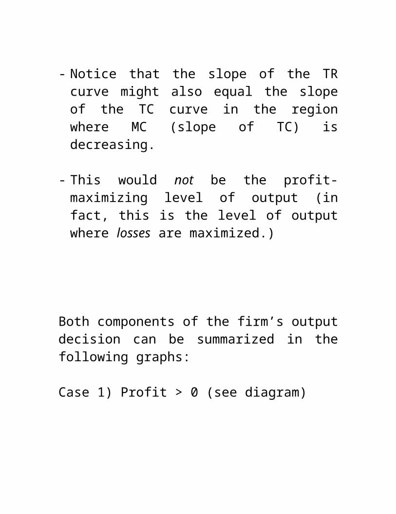
- Notice that the slope of the TR curve might also equal the slope of the TC curve in the region where MC (slope of TC) is decreasing.

- This would not be the profit-maximizing level of output (in fact, this is the level of output where losses are maximized.)

Both components of the firm’s output decision can be summarized in the following graphs:

Case 1) Profit > 0 (see diagram)

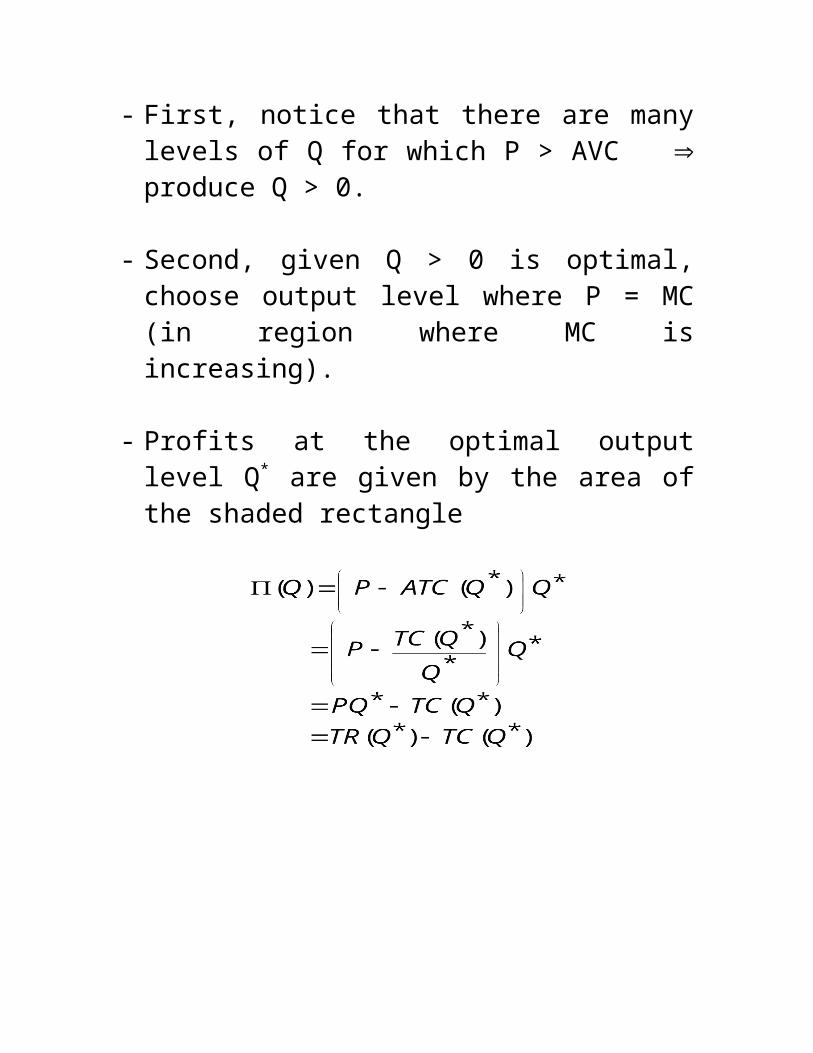
- First, notice that there are many levels of Q for which P > AVC produce Q > 0.

- Second, given Q > 0 is optimal, choose output level where P = MC (in region where MC is increasing).

- Profits at the optimal output level Q* are given by the area of the shaded rectangle

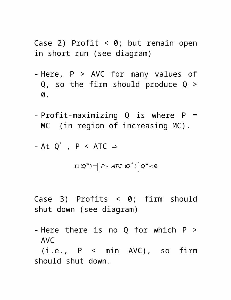
Case 2) Profit < 0; but remain open in short run (see diagram)

- Here, P > AVC for many values of Q, so the firm should produce Q > 0.

- Profit-maximizing Q is where P = MC (in region of increasing MC).

- At Q* , P < ATC

Case 3) Profits < 0; firm should shut down (see diagram)

- Here there is no Q for which P > AVC (i.e., P < min AVC), so firm should shut down.

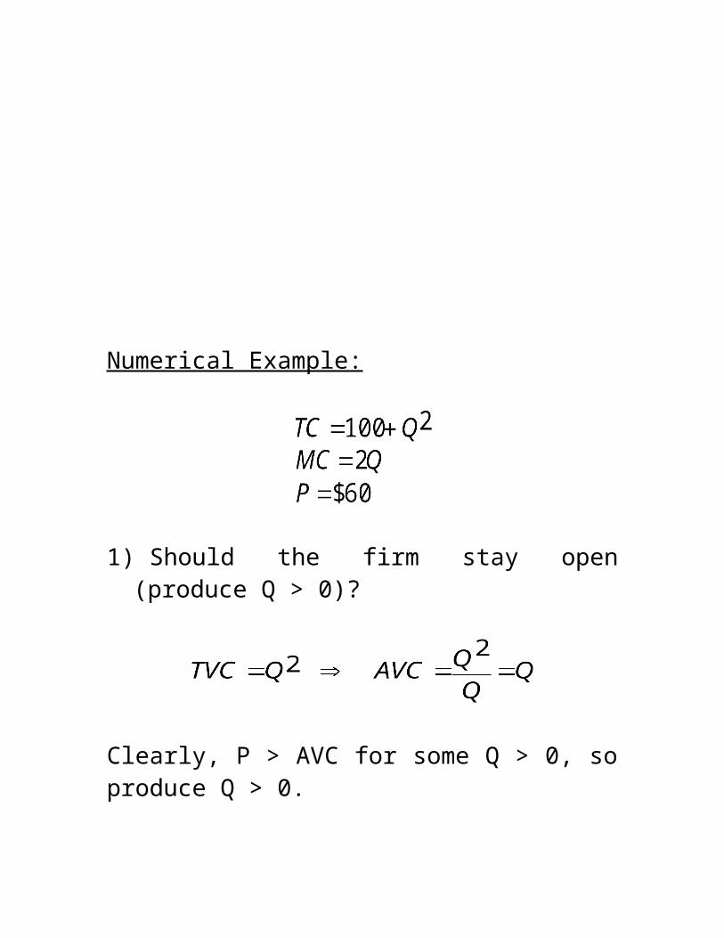
Numerical Example:

1) Should the firm stay open (produce Q > 0)?

Clearly, P > AVC for some Q > 0, so produce Q > 0.

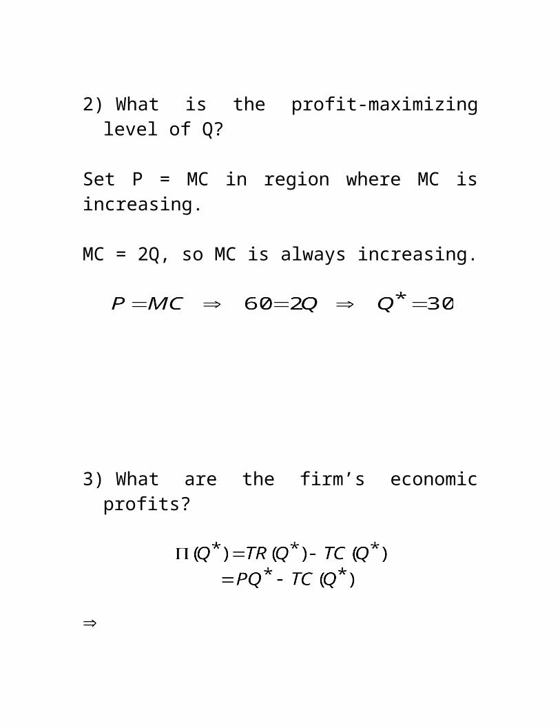
2) What is the profit-maximizing level of Q?

Set P = MC in region where MC is increasing.

MC = 2Q, so MC is always increasing.

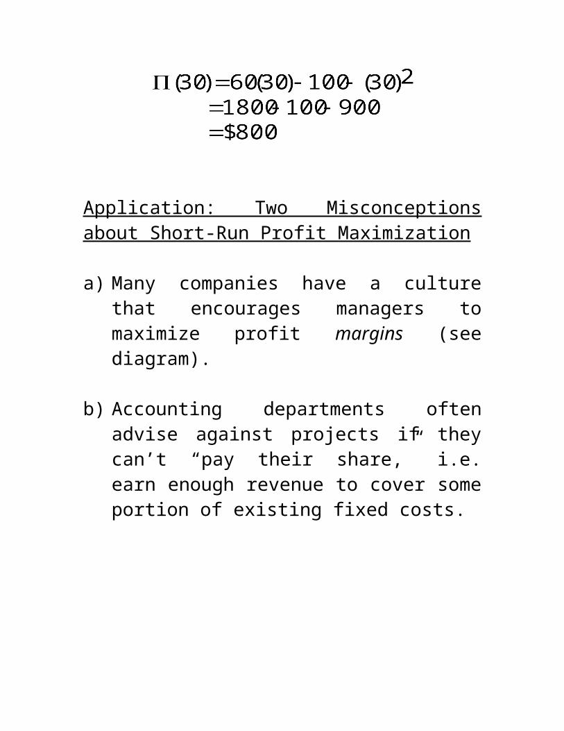
3) What are the firm’s economic profits?

Application: Two Misconceptions about Short-Run Profit Maximization

a) Many companies have a culture that encourages managers to maximize profit margins (see diagram).

b) Accounting departments often advise against projects if they can’t “pay their share,” i.e. earn enough revenue to cover some portion of existing fixed costs.

Example: Meat packing company my father worked for.

Current Production:TR = $30,000,000TVC = $10,000,000TFC = $15,000,000

Proposed Project (to be housed in unused basement):TR = $2,000,000TVC = $1,000,000

Rejected because it was assigned a 10% share of the existing fixed costs ($1,500,000).

The Firm’s Short-Run Supply Curve

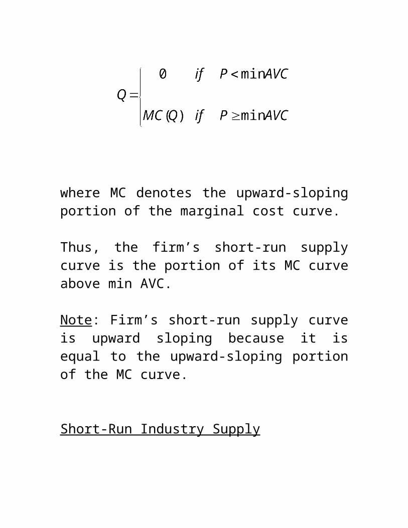
The two conditions for profit maximization define the firm’s short-run supply curve (see diagram)

where MC denotes the upward-sloping portion of the marginal cost curve.

Thus, the firm’s short-run supply curve is the portion of its MC curve above min AVC.

Note: Firm’s short-run supply curve is upward sloping because it is equal to the upward-sloping portion of the MC curve.

Short-Run Industry Supply

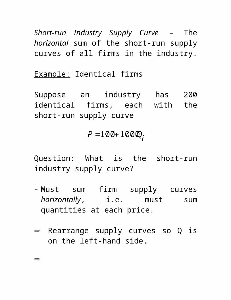
Short-run Industry Supply Curve – The horizontal sum of the short-run supply curves of all firms in the industry.

Example: Identical firms

Suppose an industry has 200 identical firms, each with the short-run supply curve

Question: What is the short-run industry supply curve?

- Must sum firm supply curves horizontally, i.e. must sum quantities at each price.

Rearrange supply curves so Q is on the left-hand side.

With 200 firms, summing the above supply curve is equivalent to multiplying it by 200, i.e.

Finally, rearrange so P is on the left-hand side

(III) Short-Run Competitive Equilibrium

As you know from your earlier economics courses, equilibrium in a given market occurs where the

market supply curve intersects the market demand curve.

Recall that the market demand curve is just the sum of the individual consumer demand curves.

Similarly, the market supply curve is the sum of the individual firm supply curves (MC curve above min AVC).

Example: Calculation of Short-Run Equilibrium

Consider a market composed of 10 identical firms, each with the cost curves given below

Assume the market demand curve takes the form

Question: What is the equilibrium price and quantity in this market?

Step 1) Calculate each firm’s short-run supply curve.

Since TVC = Q2, AVC = Q and min AVC = 0.

Thus, each firm’s short run supply curve is their MC above 0: P = 2Q.

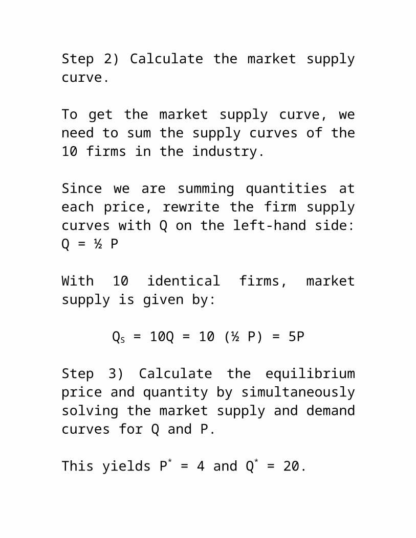
Step 2) Calculate the market supply curve.

To get the market supply curve, we need to sum the supply curves of the 10 firms in the industry.

Since we are summing quantities at each price, rewrite the firm supply curves with Q on the left-hand side: Q = ½ P

With 10 identical firms, market supply is given by:

QS = 10Q = 10 (½ P) = 5P

Step 3) Calculate the equilibrium price and quantity by simultaneously solving the market supply and demand curves for Q and P.

This yields P* = 4 and Q* = 20.

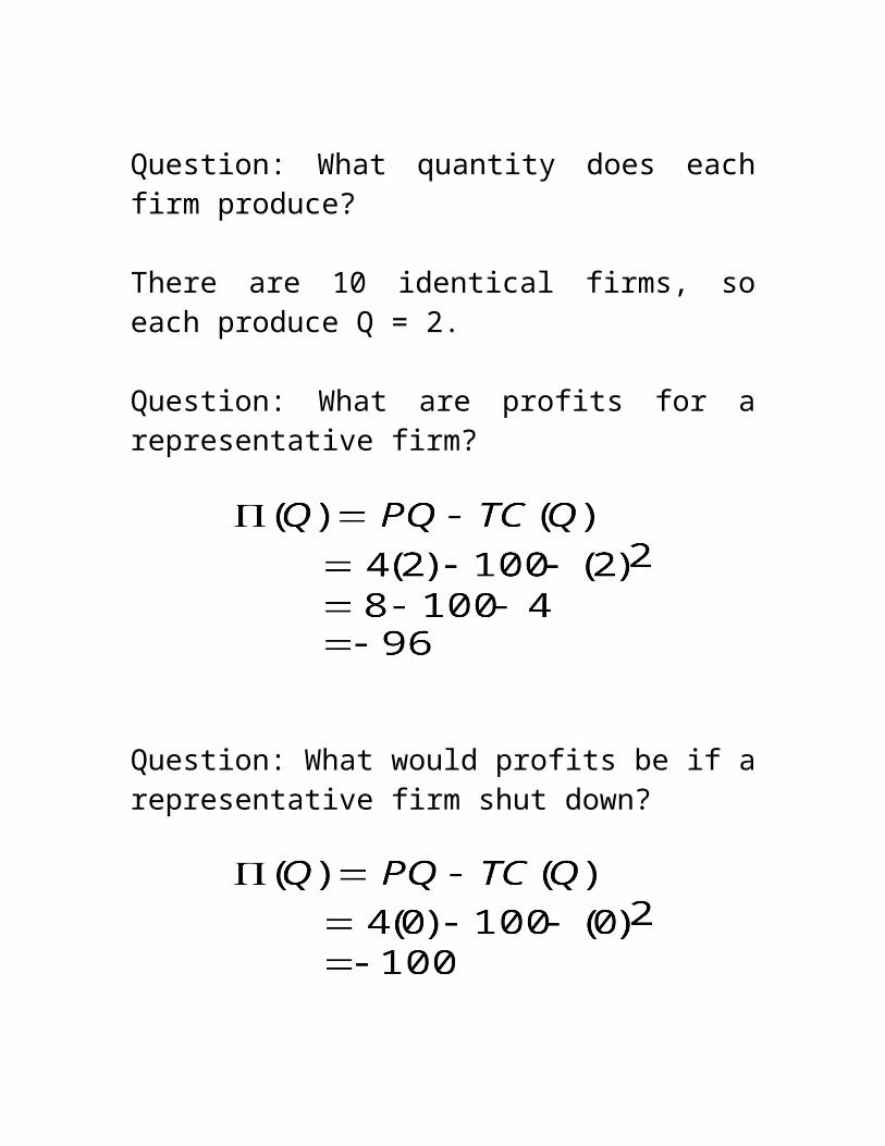
Question: What quantity does each firm produce?

There are 10 identical firms, so each produce Q = 2.

Question: What are profits for a representative firm?

Question: What would profits be if a representative firm shut down?

better off to stay open and produce Q = 2.

Efficiency of short-run competitive equilibrium

Pareto Efficiency – A condition in which all possible gains from exchange are realized.

Result: A short-run competitive equilibrium is Pareto efficient.

Reason:

- Supply curve measures marginal cost to society of producing each unit of output.

- Demand curve measures the marginal value (marginal benefit) to society of producing each unit of output (as measured by the price consumers are willing to pay).

- In a competitive equilibrium, all units of output for which the marginal value exceeds the marginal cost are produced (see diagram).

- Thus, reducing output by one unit would create an unrealized gain for society and increasing output by one unit would create a net loss for society.

IV) Long-Run Profit Maximization

In the long run, firms can adjust fixed inputs (capital) to minimize the costs of producing the desired level of output.

Firms operate on their long-run average and marginal cost curves

In the long run, all costs are variable.

ATC = AVC = LRAC (long-run average cost)

Still two components to choosing the profit-maximizing level of output:

1) Should we produce any output at all (i.e. remain in the industry)?

2) If we remain in the industry, how much output should we produce?

1) Should we remain in the industry?

If there exists some Q > 0 such that economic profits are greater than or equal to zero, i.e. if

then the firm should remain in the industry.

If not (if economic profits are negative), it means that at least one of the inputs is more highly valued in another industry.

2) If we remain in the industry, how much output should we produce?

The rule is the same as before:

Choose the level of output such that P = LRMC (in the region where LRMC is increasing) (see diagram)

V) Long-Run Competitive Equilibrium

Fact 1: Entry and exit by firms guarantees that in long-run competitive equilibrium economic profits must be zero.

Fact 2: Firms operate on their long-run cost curves.

Facts 1 and 2 imply that in a long-run competitive equilibrium, firms produce where

P = LRMC = min LRAC

(see diagram)

Reason: (see diagram)

If P > min LRAC, economic profits would be positive and firms would enter, thereby driving down the price.

If P < min LRAC, economic profits would be negative and firms would exit, thereby driving up the price.

Application – Reparations for Slavery

Q: Who should pay? (Robert Fogel’s argument).

Example: Calculation of Long-Run Equilibrium

Consider 4 identical firms, each with the cost curves shown below

Note: Observe that we don’t require any information on the demand side of the market!

Question: What is the long-run equilibrium price and quantity in this market?

It helps to draw the picture for a representative firm (see diagram).

Since there are 4 identical firms, each producing 1 unit of output, the equilibrium quantity is 4.

To find the equilibrium price, use the fact that, for each firm, P = LRMC = LRAC at the profit-maximizing output level Q = 1.

Thus, substitute Q = 1 into either LRMC or LRAC to get P* = 2.

Question: What are profits for a representative firm?

as must be true in long-run competitive equilibrium.

Efficiency Properties of Long-Run Competitive Equilibrium

1) Pareto Efficiency – all gains from trade are realized (since MB = P = LRMC).

2) Productive Efficiency – output is produced at the lowest possible unit cost (since each firm produces at the min of LRAC).